THE PERFORMANCE OF INVERSEPROBABILITY OF TREATMENT

WEIGHTING AND PROPENSITY SCOREMATCHING FOR ESTIMATINGMARGINAL HAZARD RATIOS

By Jonatan Nåtman

Department of Statistics

Uppsala University

Supervisor: Harry Khamis

2019

ABSTRACT

Propensity score methods are increasingly being used to reduce the effect of measured con-

founders in observational research. In medicine, censored time-to-event data is common. Using

Monte Carlo simulations, this thesis evaluates the performance of nearest neighbour matching

(NNM) and inverse probability of treatment weighting (IPTW) in combination with Cox pro-

portional hazards models for estimating marginal hazard ratios. Focus is on the performance

for different sample sizes and censoring rates, aspects which have not been fully investigated in

this context before. The results show that, in the absence of censoring, both methods can reduce

bias substantially. IPTW consistently had better performance in terms of bias and MSE com-

pared to NNM. For the smallest examined sample size with 60 subjects, the use of IPTW led to

estimates with bias below 15 %. Since the data were generated using a conditional parametri-

sation, the estimation of univariate models violates the proportional hazards assumption. As a

result, censoring the data led to an increase in bias.

Keywords: Monte Carlo simulations, propensity score, survival analysis, Cox model, censor-

ing rate, sample size

Contents

1 Introduction 1

2 Background 2

2.1 Causal Inference and the Potential Outcome Framework . . . . . . . . . . . . 2

2.2 Propensity Score Methods . . . . . . . . . . . . . . . . . . . . . . . . . . . . 3

2.2.1 Matching on the Propensity Score . . . . . . . . . . . . . . . . . . . . 4

2.2.2 Inverse Probability of Treatment Weighting . . . . . . . . . . . . . . . 5

2.3 Survival Analysis and the Cox Proportional Hazards model . . . . . . . . . . . 5

2.4 Previous Research . . . . . . . . . . . . . . . . . . . . . . . . . . . . . . . . . 7

3 Methodology 7

3.1 Data Generating Processes . . . . . . . . . . . . . . . . . . . . . . . . . . . . 8

3.1.1 Scenario A . . . . . . . . . . . . . . . . . . . . . . . . . . . . . . . . 8

3.1.2 Scenario B . . . . . . . . . . . . . . . . . . . . . . . . . . . . . . . . 9

3.1.3 Scenario C . . . . . . . . . . . . . . . . . . . . . . . . . . . . . . . . 9

3.1.4 Censoring Times . . . . . . . . . . . . . . . . . . . . . . . . . . . . . 9

3.1.5 Conditional Treatment Effect . . . . . . . . . . . . . . . . . . . . . . . 9

3.2 Simulation Design . . . . . . . . . . . . . . . . . . . . . . . . . . . . . . . . 10

3.3 Estimation . . . . . . . . . . . . . . . . . . . . . . . . . . . . . . . . . . . . . 11

4 Results 12

5 Discussion 19

2

1 Introduction

Randomised control trials (RCTs) are generally seen as the gold standard in medical research.

If treatment assignment is random, the treatment status should not be confounded with either

measured or unmeasured baseline characteristics. In some situations randomised controlled

studies cannot be conducted for ethical reasons. Research based on observational data also has

several advantages compared to randomised studies. The study subjects have not undergone

a strict selection procedure and might be more representative of the reality. The increasing

amount of register data also makes it possible to conduct medical studies at a lower cost, partic-

ularly when studying rare events or if long follow-up times are needed. The main disadvantage

of observational studies where the treatment assignment has not been randomised is the risk of

confounders that can make causal inference difficult.

Propensity score methods are increasingly being used to minimise the effects of confound-

ing when using observational data to estimate the effect of different treatments or exposures.

Censored time-to-event data are common in medical research. The effect of a treatment on

survival is often described with both a relative and an absolute measure in the biomedical lit-

erature, where hazard ratios and survival curves are the most commonly used measures. In

recent years, the performance of different propensity score methods to estimate hazard ratios

and survival curves have been examined in several simulation studies. These studies have fo-

cused on relatively large samples of 1000 or 10 000 subjects. Propensity score methods are

typically used in register based research where large amounts of data are available. However,

these methods are also often used for substantially smaller samples, for example when studying

patient groups with rare diseases. Also, the effect of censoring have not been fully investigated

in previous studies.

The aim of this thesis is to examine the performance of the most commonly used propen-

sity score methods in combination with Cox proportional hazards model to estimate marginal

hazard ratios. The main research question is "What is the behaviour of bias and MSE of 1:1

greedy nearest neighbour matching, with and without calipers, and inverse probability of treat-

ment weighting, when estimating marginal hazard ratios? We will focus on the performance

for different sample sizes and different censoring rates. When estimating the propensity scores,

four different models will be considered: i) a model including only the true confounder(s), ii)

a model including all variables related to outcome, iii) a model including all variables related

to treatment selection, and iiii) a model including all variables related to either outcome or

1

treatment selection. As a second question we will examine which of these models results in

estimates of marginal hazard ratios with the lowest bias and MSE.

The outline of the thesis is as follows. Section 2 provides an introduction to the theoretical

framework of this thesis. First, the potential outcome framework is presented followed by a

description of the propensity score methods. In the second part of section 2, the Cox propor-

tional hazards model is presented. Finally, a brief review of the previous research on propensity

score methods to estimate marginal hazard ratios is given. Section 3 describes the design of the

simulation study, followed by a presentation of the results in section 4. In the final part, section

5, the results are summarised and discussed.

2 Background

2.1 Causal Inference and the Potential Outcome Framework

The Rubin causal model and the concept of potential outcomes was introduced by Rubin1. Let

Zi denotes the treatment status of a subject ( Zi = 0 if the subject was assigned to the control

group and Zi = 1 if the subject received the treatment). This framework then assumes that

each subject has two potential outcomes. The first potential outcome, Yi(0), is the outcome

that would have been observed if the subject did not receive the treatment. The second, Yi(1),

is the outcome that would have been observed if the subject received the treatment. For each

subject, the individual treatment effect could then be defined as the difference between the two

potential outcomes: π1 = Yi(0)− Yi(1). However, only one of the potential outcomes can be

observed.

The average treatment effect (ATE) is the average effect of moving an entire population

from untreated to treated, expressed as E[Yi(0) − Yi(1)]. A different measure of the effect is

the treatment effect for the treated (ATT), E[Yi(0)−Yi(1)|Z = 1]. This measure describes the

average treatment effect in the population that was ultimately treated. In a randomised study,

the two measures will be equal. In an observational study however, there is no reason to expect

the ATE and ATT to be equal and which of the two measures is of greater interest depends on

the study question.

With time-to-event data, the average treatment effect would be the mean difference in sur-

vival times that results from the treatment. However, medical researchers are often more in-

terested in measures such as the difference in the probability of observing an event within a

2

specified follow-time or in the relative effect described by hazard ratios. In this thesis, which

focuses on estimating hazard ratios, we will use Austin’s2 modified definitions of ATE and

ATT. In the following sections, ATE will refer to the hazard ratio that would have been ob-

tained by regressing the hazard function on a treatment indicator in a dataset consisting of both

potential outcomes of all subjects. Similarly, ATT will be used to refer to the same analysis but

restricted to the population of subjects that actually received the treatment.

2.2 Propensity Score Methods

The propensity score is the probability of treatment assignment conditional on observed base-

line characteristics, ei = Pr(Zi = 1|Xi). Rosenbaum and Rubin3 showed that adjustment for

the propensity score is sufficient to remove bias due to measured confounders. In an obser-

vational study the propensity score is generally unknown and needs to be estimated. Several

methods can be used but the most common is estimation using logistic regression.

There is a discussion on how to select the propensity score model. The advice by Rubin

and Thomas4 is to include all variables that are related to the outcome, regardless of whether

they are related to exposure. Variables that are related only to exposure should not be included.

This is also the conclusion from two simulation studies5,6. This strategy for variable selection

might seem counter-intuitive but has been motivated by the notion that even if a variable is

theoretically unrelated to the exposure, there is a possibility that it is related to the exposure

by chance in the dataset. If that is the case, the variable will be a confounder in that particular

dataset. On the other hand, including a variable that is strongly related to treatment selection

but unrelated to the outcome will induce variability to the propensity score model that does not

correct for confounding5 .

When the propensity score has been estimated, there are four broad methods to adjust for it:

matching on the propensity score, stratification on the propensity score, covariate adjustment

using the propensity score and inverse probability of treatment weighting (IPTW)3,7. All of

these methods have been applied to survival data and have recently been evaluated in simula-

tion studies. It has been showed that matching and IPTW estimate marginal effects whereas

stratification and covariate adjustment estimate conditional effect8,9. Therefore, this thesis will

focus on propensity score matching and IPTW.

3

2.2.1 Matching on the Propensity Score

Matching on the propensity score means that a matched set is formed of treated and untreated

subjects that have similar values of the propensity score. There are several ways to implement

propensity score matching and Austin2 gives a good overview of different algorithms. The

most common implementation is to form pairs of treated and control subjects, which is called

one-to-one (1:1) matching. Another approach is one-to-many (1:M), where one treated subject

is matched to two or more control subjects. Full matching is another method that makes use

of all individuals in the data by forming matched sets of one treated subject and one or more

controls. Full matching can estimate both ATE and ATT whereas 1:1 matching always targets

ATT2. We will focus only on 1:1 matching, which is the most commonly used method for

propensity score matching.

A matching algorithm also needs to be chosen. The two most common are optimal match-

ing and greedy nearest neighbour matching (NNM)2. The first aims to minimise the average

difference in propensity score within the matched pairs. The latter, on the other hand, finds one

treated subject and then selects the untreated subject with closest propensity score as control.

The greedy matching algorithm chooses the order in which the treated subjects are matched

either randomly, sequentially from lowest to highest propensity or from highest to lowest, or

by the order of how close the best match is.

It is also common to put restrictions on the quality of the matches. This is called nearest

neighbour matching with calipers. Caliper matching is similar to NNM but if there is no un-

treated subject with a propensity score within a specified distance from the selected treated sub-

ject, the treated subject will not be included in the matched sample and the analysis. Austin10

recommends using a caliper of 0.2 standard deviations of the logit of the propensity score. The

choice of using calipers or not represents a trade off between two sources of bias. If no re-

strictions are put on the quality of the matches, or if the calipers are wide, the distribution of

propensity scores between the treated group and the control group might still differ substan-

tially after matching. If calipers are used, some treated subjects might get excluded from the

analysis and thus changing the target population.

Austin11 compared several different 1:1 matching algorithms in a simulation study where

differences in means were estimated. It was found that optimal matching had no advantage

over greedy NNM in achieving balance in the baseline covariates. NNM with calipers resulted

in estimates with less bias but slightly higher variability than NNM without restriction. For

4

greedy NNM, the order in which the treated subjects were selected did not have any particular

effect on estimation. Also, matching with replacement did not have better performance than

matching without replacement. Based on this, they recommend using NNM with calipers and

random order.

Two different methods for matching will be evaluated in this study: 1:1 greedy nearest

neighbour matching, with and without calipers.

2.2.2 Inverse Probability of Treatment Weighting

Inverse probability of treatment weighting (IPTW) uses the propensity score to compute weights.

These weights are used to construct a synthetic sample where the distribution of measured co-

variates is independent of treatment assignment. The weights can be chosen so they represent

different target populations, either to target the ATE or the ATT. We will focus on the ATT

weights since this is the measure that the 1:1 matching targets. Let Zi be the treatment indi-

cator and ei be the estimated propensity score for the ith subject . The ATT weights are then

given by

wi = Zi +ei(1− Zi)(1− ei)

. (1)

Thus, all treated subjects are given a weight of 1 and the subjects in the control group are

given a weight of ei/(1− ei).

2.3 Survival Analysis and the Cox Proportional Hazards model

Survival analysis, also called time-to-event analysis, is a collection of statistical procedures for

analysing data where the variable of interest is the time until an event occurs. The event of

interest can be for example death or relapse from remission. A common feature of these data is

that observations are censored. Censoring is a type of missing data problem that can occur due

to several reasons. In medicine, a frequent type is right censoring which means that all that is

known is that subject is still alive at a given time. Right censoring can for example occur when

the study is terminated before all subjects have experienced the event or if a subject leaves the

study before having experienced the event. Then we will only know that the subject was still

alive when it was censored but not the time when the event was experienced.

When analysing the effect of a treatment, usually both an absolute and a relative measure

of the effect is of interest. The techniques that are most commonly used to deal with censored

5

time-to-event data is the Kaplan-Meier estimator, which estimates the survival function, and

Cox proportional hazards (PH) model, which is used to model the effect of covariates on the

hazard rate. The hazard function is defined

h(t) = lim∆t→0

P[t ≤ T < t+ ∆t|T ≥ t]

∆t(2)

which is the probability that a subject will not survive for an additional time ∆t given that

it has survived until time t.

In the Cox PH model12, the effect of a one unit increase in a covariate has a multiplicative

effect on the hazard rate

h(t;X) = h0(t)eθZ+Xβ (3)

where h(t;X) is the hazard function at time t, h0(t) is the baseline hazard, θ is the treatment

effect, Z the treatment indicator, X is a vector of covariates and β is a vector of parameters.

The Cox PH model is semi-parametric since the functional form of the baseline hazard does

not need to be specified.

In the Cox model, θ is the treatment effect conditional on the covariates X. A measure of

an effect is said to be collapsible if the marginal and the conditional effect coincide in absence

of confounding13. That is true for linear models but not for hazard ratios or odds ratios in

general14. Regardless of whether X is related to Z, controlling for X will infer different

estimands. While conditional effects denote an average effect at the individual level, marginal

effects denote an effect at the population level. Thus, the marginal effect is the hazard ratio

of two identical populations, except that in one population all subjects received treatment and

in the other everyone was untreated. In that sense, adjusting for covariates at the design stage

by propensity score methods and controlling for the covariates in the regression analysis will

estimate different effects.

A key assumption of the Cox PH model is the proportional hazard assumption, meaning

that the effect of a covariate is constant over time. Chastang et al.15 showed that omission of

a covariate in a Cox PH model can cause bias, even if the covariate is completely balanced

between the treatment and the control groups. This results from the hazards in the two groups

no longer being proportional if a prognostic variable is omitted from the model. Even when the

PH assumption is violated, the estimate from a Cox model can still be useful. It can be seen as

6

a geometric average of the treatment effect over the support of the data. However, this estimate

will be a function of the distribution of censoring times16.

2.4 Previous Research

Gayat et al.8 evaluate the performance of stratification on the propensity score, covariate ad-

justment using the propensity score and propensity score matching. They concludled that the

methods, except matching, estimated conditional effects rather than marginal effects. How-

ever, matching on the propensity score gave unbiased estimates of the marginal hazard ratio.

The methods were evaluated with sample sizes of 1000 subjects and a censoring rate of 40 %.

They also investigated the effect of an unmeasured confounder. The unmeasured confounder

led to substantially biased estimates but replacing the unmeasured confounder with a highly

correlated variable could remove most of the bias.

Austin9 compares the performance of IPTW and propensity score matching for estimat-

ing marginal hazard ratios in a simulation study of several scenarios of different hazard ratios

and prevalences of exposure. It was found that both methods yield approximately unbiased

estimates of the effect in the treated population. IPTW had lower mean squared errors and

the difference between the methods increased when the prevalence of exposure was low. The

methods were evaluated in samples of 10 000 subjects and the data were not censored.

Pirracchio et al.6 examined the performance of IPTW and propensity score matching for

estimation of odds ratios in case of small samples. They found that both methods could yield

estimates with less than 10 % bias for sample sizes from 1000 down 40 subjects. IPTW had

better performance of bias and MSE except when the sample size was 40. For the smallest

sample size, matching yielded estimates with slightly lower bias.

3 Methodology

A Monte Carlo simulation study was performed to evaluate the behaviour of bias and MSE

when using propensity score methods to estimate marginal hazard ratios. To examine the per-

formance of the methods under different conditions, we used three slightly modified data gen-

erating processes to represent different situations. These simulated situations will be referred

to as Scenario A, B and C. In each scenario, samples of different sizes were generated. Also,

censoring times were simulated from different distributions. In each simulated data set, the

7

propensity score methods were applied separately and marginal Cox PH models were fitted.

The estimates were compared to the true treatment effect. Here follows a detailed description

of the simulation design and the estimation methods.

3.1 Data Generating Processes

3.1.1 Scenario A

Three baseline covariates, X1, X2 and X3, were simulated from independent standard normal

distributions. Of these, the first two affected treatment selection whereas the last two affected

the outcome. Thus, X2 is the only true confounder.

Each subject’s probability of being assigned to treatment was simulated using a logistic model

logit(pi) = log(α0) + log(α1)x1i + log(α2)x2i (4)

where α1 = α2 = 2 and α0 was chosen so that 30% of the subjects were treated. The treat-

ment status for each subject was then generated from a Bernoulli distribution with individual

parameter pi.

The event times were generated following the technique described by Bender et al.17. First,

a linear predictor was defined

LPi = θZi + log(β2)x2i + log(β3)x3i (5)

.

where β2 and β3 also were set to 2. These parameters were chosen so that the variables

should have a substantial impact on treatment selection and/or outcome.

The time-to-event, T, was simulated by inverting the cumulative hazard function of a

Weibull distribution,

Ti =

(−log(ui)

λexp(LPi)

)1/η

(6)

where ui ∼ U(0, 1). The scale parameter λ and the shape parameter η were set to 2 and

0.00002 respectively, as have been done in other studies9,18.

8

3.1.2 Scenario B

In Scenario B, a second confounder was added. Four variablesX1, ..., X4, were simulated from

independent standard normal distributions. Now, X1, ..., X3 affected treatment selection and

X2, ..., X4 affected the outcome. Thus, X2 and X3 are confounders.

The probability of assignment was simulated as in Scenario A, but adding the third variable

to the data generating process

logit(pi) = log(α0) + log(α1)x1i + log(α2)x2i + log(α3)x3i (7)

.

Also in this scenario, α0 was chosen so that 30% of the subjects received treatment. Event

times were generated as in Scenario A, with the variable X4 added to the linear predictor

LPi = θZi + log(β2)x2i + log(β3)x3i + log(β4)x4i (8)

.

Again, the parameters α1, ..., α3 and β2, ..., β4 were set to 2.

3.1.3 Scenario C

Scenario C is also a slightly modified version of Scenario A. However, α0 was changed so that

10% of the subjects received treatment. In all other aspects, the data generating processes were

the same as in Scenario A with three simulated variables of which one was a true confounder.

3.1.4 Censoring Times

To simulate censoring times Ci, two different distributions were used. First, censoring was

simulated from the Weibull distribution. The shape parameter η was set to 0.00002 and the

scale parameter λ was changed to obtain the desired censoring rate. A uniform distribution was

also considered, where Ci ∼ unif(0, b), changing the parameter b to obtain different rates.

3.1.5 Conditional Treatment Effect

Since the survival times were generated from a conditional model, exp(θ) is the conditional

treatment effect. An iterative bisection method was used to determine the conditional effect

9

Table 1: Summary of simulation settings

Scenario Data generating process Number ofconfounders

Samplesizes

Prevalenceof treatment

A logit(pi) = α0 + log(2)x1i + log(2)x2i 1 60,...,1000 30 %LPi = θZi + log(2)x2i + log(2)x3i

B logit(pi) = α0 + log(2)x1i + log(2)x2i + log(2)x3i 2 60,...,1000 30 %LPi = θZi + log(2)x2i + log(2)x3i + log(2)x4i

C logit(pi) = α0 + log(2)x1i + log(2)x2i 1 180,...,3000 10 %LPi = θZi + log(2)x2i + log(2)x3i

that induced the desired marginal hazard ratio. This method is described in detail by Austin to

generate data with a specified marginal odds ratio and has also been applied to hazard ratios9,19.

Briefly, a data set of 1000 subjects was simulated. For each treated subject, the two potential

outcomes were generated as described above. However, the survival times were not censored

since it most often is the true uncensored effect that is of scientific interest. Survival times

were then regressed on the treatment indicator using Cox regression. Over 10 000 replications,

the mean of the parameter estimates was taken as the true marginal hazard ratio in the treated

population corresponding to the conditional effect θ. We then searched for the value of θ that

gave the desired marginal hazard ratio.

3.2 Simulation Design

The true marginal hazard ratio was chosen to be 1.5. This was obtained by setting the condi-

tional hazard ratio exp(θ) ≈ 1.859 in Scenario A, exp(θ) ≈ 1.983 in Scenario B and exp(θ) ≈

1.864 in Scenario C. Seven different censoring distributions were simulated: the situation of no

censoring and censoring rates of 20% , 40% and 50% from uniform and Weibull distributions,

respectively. In each combination of censoring distribution and Scenario A-C, samples of dif-

ferent sizes were generated. In Scenario A and B, the samples ranged from 1000 down to 60

subjects (n = 1000, 900, 800, 700, 600, 500, 400, 300, 200, 180 , 160, 140, 120, 100, 80, 60).

In order to get a reasonable number of observations in the treated group in Scenario C, we mul-

tiplied the total sample sizes by three (n ranging from 3000 down to 180). Thus, the expected

number of treated subject were the same as in the other two scenarios. A summary of the three

scenarios is presented in Table 1.

10

3.3 Estimation

Within each simulated data set, the propensity scores were estimated using logistic regression.

The propensity scores were estimated using four different models: a model including only the

true confounder(s) (M1), a model including the variables related to outcome only (M2), a model

including the variables related to treatment selection only (M3) and finally a model including

all variables related to either outcome or treatment (M4).

The three different propensity score methods were applied: i)1:1 greedy nearest neigh-

bour matching (NNM), ii) 1:1 greedy nearest neighbour matching within a caliper 0.2 st.d. of

the logit of the propensity score (Caliper matching) and iii) inverse probability of treatment

weighting (IPTW). In the matched samples, a univariate Cox PH model was used to regress

time-to-event on the treatment indicator. For IPTW, a Cox PH model was also used to regress

time-to-event on the treatment indicator, including the ATT weights as sample weights. For

comparison, also an unadjusted model in the original sample was estimated (crude model), as

well as a correctly specified conditional model (adjusted model). Since we suspect that the

marginal hazards might violate the PH assumption we will check the proportionality by also

estimating hazard ratios for different time intervals.

The methods were evaluated with relative bias and mean squared error (MSE) on the log-

hazard scale

Bias =1

5000

5000∑i=1

δ̂i − δδ

(9)

MSE =1

5000

5000∑i=1

(δ̂i − δ)2 (10)

where δ̂i is the estimated log-hazard ratio of the ith simulated dataset and δ is the true

marginal log-hazard ratio in the treated population. When evaluating the conditional model, δ

was defined as the true conditional effect.

All simulations were performed in R version 3.5.1. The function glm was used to fit logistic

regressions to estimate the propensity scores. The function Match in the package Matching was

used for matching on the propensity score. To estimate Cox proportional hazard models, coxph

in the survival package was used.

11

4 Results

For each propensity score method, four different logistic models were considered when es-

timating the propensity score: a model including only the true confounder(s) (M1), a model

including all variables related to the outcome (M2), a model including all variables related to

treatment selection (M3) and a model including all variables related to either treatment selec-

tion or outcome (M4). In terms of bias, the differences between the four models were small

for Caliper matching and IPTW. M1 and M2 had slightly lower bias than M3 and M4. The

differences between the models were larger for NNM, where M1 and M2 produced less biased

estimated than did M3 and M4. There were however no large differences between M1 and

M2. When comparing MSE, M2 was better than the other three models in all cases but a few

exceptions across all simulations. There were no clear patterns in the relative performance of

the four models across the three simulated scenarios, sample sizes or censoring distributions.

In the remainder of this thesis, we will focus on the results produced by the model including all

variables related to the outcome, M2.

Table 2 shows some descriptive statistics, averaged over the 5000 Monte Carlo replica-

tions, that describes the quality of the matching methods and the IPTW. Since censoring does

not have any impact on the estimation of the propensity scores, only the results for the data

simulated in the case of no censoring are presented. First, in Scenario A with n = 1000,

95.7 % of the the treated subjects were successfully matched to a control subject with similar

propensity score when calipers were applied. As the sample size decreases, so does the share

of matched subjects. Thus, there is a relatively low risk of bias due to incomplete matching

when n = 1000, but the risk increases as the sample size decreases. In Scenario B, where a

second confounder is added, a lower share of the subjects are matched compared to Scenario

A with only one confounder. In Scenario C, 10 % of the subjects received the treatment. The

relatively larger number of control subjects makes it easier to find a match within the specified

calipers. Compared to Scenario A, only a small number of treated subjects are excluded from

the analysis. In NNM, all treated subjects are included in the analysis. Without any restriction

on the quality of the matches, there are no guarantees that the distribution of the covariates

will be similar in the matched sample. The second panel in Table 2 shows the difference in

means between the treated group and the control group in the matched sample, averaged over

the Monte Carlo replications. The variable that is related to treatment only is not included in

the propensity score model and the imbalance between the groups remains after matching. The

12

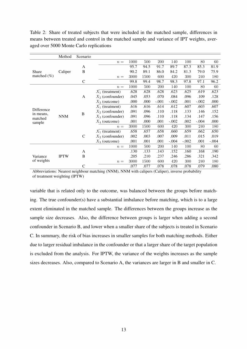
Table 2: Share of treated subjects that were included in the matched sample, differences inmeans between treated and control in the matched sample and variance of IPT weights, aver-aged over 5000 Monte Carlo replications

Method Scenarion = 1000 500 200 140 100 80 60

Sharematched (%)

CaliperA 95.7 94.5 91.7 89.7 87.3 85.3 81.9B 90.2 89.1 86.0 84.2 81.3 79.0 75.9

n = 3000 1500 600 420 300 240 180C 99.8 99.4 98.7 98.3 97.8 97.1 96.2

n = 1000 500 200 140 100 80 60

Differencein means,matchedsample

NNM

AX1 (treatment) .628 .628 .628 .623 .625 .619 .623X2 (confounder) .045 .053 .070 .084 .096 .109 .128X3 (outcome) .000 .000 -.001 -.002 .001 -.002 .000

B

X1 (treatment) .616 .616 .614 .612 .607 .603 .607X2 (confounder) .091 .096 .110 .118 .133 .146 .152X3 (confounder) .091 .096 .110 .118 .134 .147 .156X4 (outcome) .001 .000 .001 -.002 .002 -.004 .000

n = 3000 1500 600 420 300 240 180

CX1 (treatment) .658 .657 .658 .660 .659 .662 .650X2 (confounder) .002 .003 .007 .009 .011 .015 .019X3 (outcome) .001 .001 .001 -.004 -.002 .001 -.004

n = 1000 500 200 140 100 80 60

Varianceof weights

IPTWA .130 .133 .143 .152 .160 .168 .190B .205 .210 .237 .246 .286 .321 .342

n = 3000 1500 600 420 300 240 180C .077 .077 .078 .078 .078 .079 .080

Abbreviations: Nearest neighbour matching (NNM), NNM with calipers (Caliper), inverse probabilityof treatment weighting (IPTW)

variable that is related only to the outcome, was balanced between the groups before match-

ing. The true confounder(s) have a substantial imbalance before matching, which is to a large

extent eliminated in the matched sample. The differences between the groups increase as the

sample size decreases. Also, the difference between groups is larger when adding a second

confounder in Scenario B, and lower when a smaller share of the subjects is treated in Scenario

C. In summary, the risk of bias increases in smaller samples for both matching methods. Either

due to larger residual imbalance in the confounder or that a larger share of the target population

is excluded from the analysis. For IPTW, the variance of the weights increases as the sample

sizes decreases. Also, compared to Scenario A, the variances are larger in B and smaller in C.

13

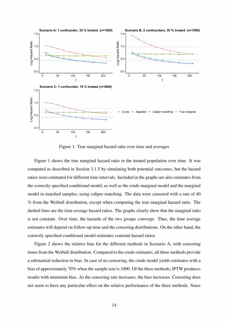
Figure 1: True marginal hazard ratio over time and averages

Figure 1 shows the true marginal hazard ratio in the treated population over time. It was

computed as described in Section 3.1.5 by simulating both potential outcomes, but the hazard

ratios were estimated for different time intervals. Included in the graphs are also estimates from

the correctly specified conditional model, as well as the crude marginal model and the marginal

model in matched samples, using caliper matching. The data were censored with a rate of 40

% from the Weibull distribution, except when computing the true marginal hazard ratio. The

dashed lines are the time average hazard ratios. The graphs clearly show that the marginal ratio

is not constant. Over time, the hazards of the two groups converge. Thus, the time average

estimates will depend on follow-up time and the censoring distributions. On the other hand, the

correctly specified conditional model estimates constant hazard ratios

Figure 2 shows the relative bias for the different methods in Scenario A, with censoring

times from the Weibull distribution. Compared to the crude estimates, all three methods provide

a substantial reduction in bias. In case of no censoring, the crude model yields estimates with a

bias of approximately 70% when the sample size is 1000. Of the three methods, IPTW produces

results with minimum bias. As the censoring rate increases, the bias increases. Censoring does

not seem to have any particular effect on the relative performance of the three methods. Since

14

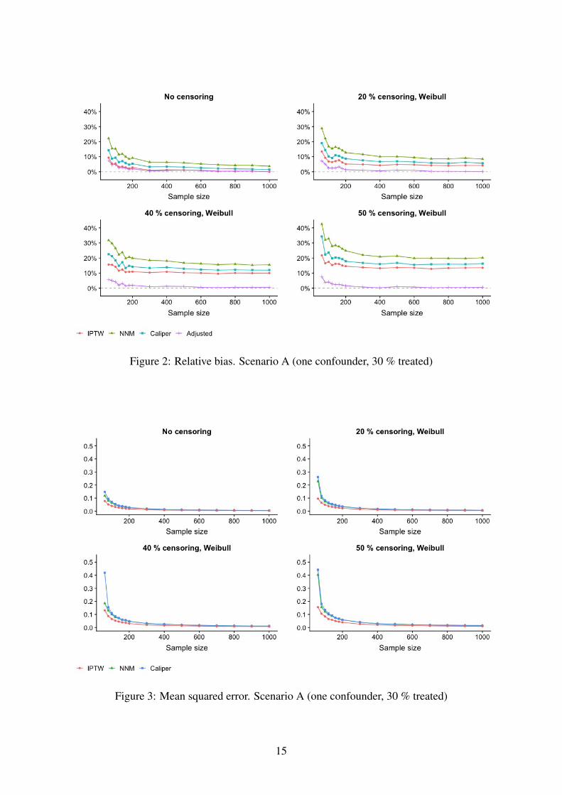
Figure 2: Relative bias. Scenario A (one confounder, 30 % treated)

Figure 3: Mean squared error. Scenario A (one confounder, 30 % treated)

15

the marginal hazards in the groups are nonproportional, the time average estimates are expected

to be a function of the censoring distribution. If subjects with longer survival times are more

likely to be censored, the hazard ratios at later time points will get a smaller weight in the

average hazard ratio. Since the hazards are convergent, this will result in overestimation of

the average hazard ratio. Similar shifts in the bias were obtained when censoring times were

simulated from a uniform distribution, however the shifts were slightly smaller. The bias of the

adjusted conditional model is not affected by the censoring distribution. Note however that this

model estimates and was compared to a different effect.

The mean squared errors for Scenario A are presented in Figure 3. Also in terms of MSE,

IPTW yields the best results. NNM and Caliper matching have similar MSE. As the sample

size gets smaller, the MSE of caliper matching increase sligtly more rapidly.

In Scenario B, where a second confounder is added, Figure 4 shows that bias increase for all

models. Also in this scenario, IPTW has the best performance for all sample sizes. Compared

to Scenario A, the use of calipers when constructing the matched sample seems to have a larger

effect on reducing the bias. Also in Scenario B, censoring of the data causes similar shifts in

the bias curves. The MSE, presented in Figure 5, shows that IPTW have the best performance

across all sample sizes. Caliper have lower MSE compared to NNM, except for the smallest

sample sizes.

Figure 6 shows the relative bias for Scenario C. Also in this scenario, IPTW has the lowest

bias. However, the differences between the three methods are small. When the sample size is

180, with 18 treated subjects on average, the bias of IPTW is 5.5 % in case of no censoring.

The MSE are presented in Figure 7. NNM and caliper matching have similar values for all

sample sizes. IPTW have the smallest MSE, approximately half of those for NNM and caliper

matching, and the difference gets larger for the smallest sample sizes. Thus, the variance of

the IPTW estimates seems to be less sensitive to sample size. The bias and MSE are almost

identical for NNM and caliper matching.

More comprehensive results are available on request: jonatan.natman@gmail.com.

16

Figure 4: Relative bias. Scenario B (two confounders, 30 % treated)

Figure 5: Mean squared error. Scenario B (two confounders, 30 % treated)

17

Figure 6: Relative bias. Scenario C (one confounder, 10 % treated)

Figure 7: Mean squared error. Scenario C (one confounder, 10 % treated)

18

5 Discussion

In this thesis we have evaluated the performance of inverse probability of treatment weight-

ing (IPTW) and nearest neighbour matching (NNM), with and without calipers, to estimate

marginal hazard ratios (MHR) of a treatment effect in the treated population. The methods

were evaluated based on bias and MSE in a series of simulations.

First we examined different models to estimate the propensity score. It was confirmed

that for all three propensity score methods, the model that included all variables related to the

outcome, regardless of whether they were confounders, had the best performance. These results

are in agreement with other simulation studies5,6. All further comparisons of the propensity

score methods were based on this model.

The results show that the propensity score methods can adjust for measured confounders

and produce approximately unbiased estimates of MHRs in the absence of censoring. IPTW

had better performance across sample sizes and the different data-generating processes com-

pared to the matching methods, both in terms of bias and MSE. When there was one confounder,

IPTW produced estimates with bias of less than 10 % for sample sizes down to 60 subjects.

Adding a second confounder to the data-generating process resulted in slightly higher biases

for all methods. When a smaller proportion of the subjects received treatment, the differences

in bias and MSE between the methods decreased. Thus, a relatively large number of control

subjects was more important when using the matching methods. As the sample size decreased,

the bias increased for all methods. For the matching methods, it is possible that it is more

difficult to find a control subject with similar propensity score in a smaller sample. A possible

explanation for the increase in bias for IPTW could be the larger variability of the weights in

the smaller samples. Comparing the larger sample sizes, these results are in agreement with

Austin’s9 who simulated data without censoring and with sample sizes of 10 000 subjects.

When the data were censored, this introduced bias that increased with the censoring rate. It

has been showed by Chastang et al.15 that the PH assumption is violated, even if a completely

balanced covariate is omitted from the Cox PH model. When examining the proportionality of

the hazards, it was confirmed that conditional hazards were proportional whereas the marginal

hazards were convergent. This increase in bias is likely a result of the nonproportionality of the

hazards. When the hazards are nonproportional, the hazard ratios from the Cox PH regression

can be interpreted as a geometric average, weighted by the number of observations at each time

point. When the censoring rate was 50 %, the maximum increase in bias was about 15 percent-

19

age points. Gayat et al.8 simulated data with sample sizes of 1000 subjects and evaluated NNM.

With 40 % censoring rate they found, unlike this study, that it had approximately unbiased esti-

mates of the marginal hazard ratio. The differences between their results and the current study

could perhaps be due to that they took the censoring distribution into account when computing

the true marginal hazard ratio by simulating both potential outcomes and censoring the data.

Even if treatment assignment were completely randomised in a RCT, a marginal Cox model

would still yield estimates with similar bias, if the survival data came from the same conditional

model with the same distribution of censoring times. Three reviews of randomised clinical trials

recently published in oncology journals show that treatment effects are often evaluated using

marginal Cox models20–22. Also, the PH assumption was only justified or discussed in few of

the articles. As previous studies have noted, the propensity score methods estimates marginal

rather than conditional effects9. Although not specifying the correct conditional model violates

the assumptions of the Cox regression, propensity score methods can be a useful alternative to

estimate similar effects to those that are commonly reported in RCTs.

Aalen et al.23 discuss a problem of randomisation with the Cox model. Even if the treat-

ment assignment is randomised at the start of the study, this randomisation is lost by implicit

conditioning as soon has the first event occurs if the outcome model is not correctly specified.

Thus, the marginal hazards in these simulations might lack a clear causal interpretation.

There are certain limitations in this study. Since the models have been evaluated based on

simulations, it is difficult to know how generalisable the results are to other situations than the

specific settings in these simulations. For example, there could be different numbers of co-

variates or distributions of the covariates such as binary or correlated variables, different sizes

of treatment effects and other prevalences of treatment. Also, in reality it is unlikely that all

confounders are measured. However, these methods are difficult to evaluate analytically and

simulation studies are important in order to understand under which conditions the methods

work well. There are also several other matching algorithms, such as matching with replace-

ment, that perhaps could have given different results.

In summary, IPTW had consistently the lowest bias and MSE across the simulations. IPTW

and the matching methods had most similar performance when both sample size and the ratio

of the number of control to treated subjects were large. IPTW was less sensitive to sample size

and the number of control subjects.

20

References

1 Rubin D. Estimating causal effects of treatments in randomised and nonrandomised studies.

Journal of Educational Psychology. 1974 mar;66(6):688–701.

2 Austin PC. The use of propensity score methods with survival or time-to-event outcomes:

reporting measures of effect similar to those used in randomized experiments. Statistics

in Medicine. 2014 mar;33(7):1242–1258. Available from: https://www.ncbi.nlm.nih.gov/

pmc/articles/PMC4285179/.

3 Rosenbaum PR, Rubin DB. The central role of the propensity score in observational studies

for causal effects. Biometrika. 1983;70(1):41–55. Available from: https://academic.oup.

com/biomet/article/70/1/41/240879.

4 Rubin DB, Thomas N. Matching Using Estimated Propensity Scores: Relating Theory to

Practice. Biometrics. 1996 mar;52(1):249.

5 Brookhart MA, Schneeweiss S, Rothman KJ, Glynn RJ, Avorn J, Stürmer T. Vari-

able selection for propensity score models. American journal of epidemiology. 2006

jun;163(12):1149–56. Available from: https://www.ncbi.nlm.nih.gov/pubmed/16624967.

6 Pirracchio R, Resche-Rigon M, Chevret S. Evaluation of the Propensity score methods

for estimating marginal odds ratios in case of small sample size. BMC Medical Research

Methodology. 2012 dec;12(1):70. Available from: https://www.ncbi.nlm.nih.gov/pubmed/

22646911.

7 Rosenbaum PR. Model-Based Direct Adjustment. Journal of the American Statistical

Association. 1987 jun;82(398):387. Available from: https://www.jstor.org/stable/2289440.

8 Gayat E, Resche-Rigon M, Mary JY, Porcher R. Propensity score applied to survival data

analysis through proportional hazards models: a Monte Carlo study. Pharmaceutical Statis-

tics. 2012 may;11(3):222–229. Available from: http://doi.wiley.com/10.1002/pst.537.

9 Austin PC. The performance of different propensity score methods for estimating marginal

hazard ratios. Statistics in Medicine. 2013 jul;32(16):2837–2849. Available from: http:

//doi.wiley.com/10.1002/sim.5705.

21

10 Austin PC. Optimal caliper widths for propensity-score matching when estimating dif-

ferences in means and differences in proportions in observational studies. Pharmaceutical

Statistics. 2011 mar;10(2):150–161. Available from: http://doi.wiley.com/10.1002/pst.433.

11 Austin PC. A comparison of 12 algorithms for matching on the propen-

sity score. Statistics in medicine. 2014 mar;33(6):1057–69. Available from:

http://www.ncbi.nlm.nih.gov/pubmed/24123228http://www.pubmedcentral.nih.gov/

articlerender.fcgi?artid=PMC4285163.

12 Cox DR. On collapsibility and confounding bias in Cox and Aalen regression models.

Journal of the Royal Statistical Society. 1972;66(34):187–220.

13 Greenland S, Robins JM, Pearl J. Confounding and Collapsibility in Causal Inference;

1999. 1. Available from: https://projecteuclid.org/euclid.ss/1009211805.

14 Martinussen T VS. On collapsibility and confounding bias in Cox and Aalen regression

models. Lifetime data analysis. 2013 jun;66(9):279–96.

15 Chastang C, Byar D, Piantadosi S. A quantitative study of the bias in estimating the

treatment effect caused by omitting a balanced covariate in survival models. Statistics in

Medicine. 1988 dec;7(12):1243–1255. Available from: http://doi.wiley.com/10.1002/sim.

4780071205.

16 Boyd AP, Kittelson JM, Gillen DL. Estimation of treatment effect under non-

proportional hazards and conditionally independent censoring. Statistics in medicine. 2012

dec;31(28):3504–15. Available from: http://www.ncbi.nlm.nih.gov/pubmed/22763957http:

//www.pubmedcentral.nih.gov/articlerender.fcgi?artid=PMC3876422.

17 Bender R, Augustin T, Blettner M. Generating survival times to simulate Cox proportional

hazards models. Statistics in Medicine. 2005 jun;24(11):1713–1723. Available from: http:

//doi.wiley.com/10.1002/sim.2059.

18 Austin PC, Stuart EA. The performance of inverse probability of treatment weighting and

full matching on the propensity score in the presence of model misspecification when es-

timating the effect of treatment on survival outcomes. Statistical Methods in Medical Re-

search. 2017;26(4):1654–1670.

22

19 Austin PC, Stafford J. The Performance of Two Data-Generation Processes for Data with

Specified Marginal Treatment Odds Ratios. Communications in Statistics - Simulation and

Computation. 2008 may;37(6):1039–1051. Available from: http://www.tandfonline.com/

doi/abs/10.1080/03610910801942430.

20 Rulli E, Ghilotti F, Biagioli E, Porcu L, Marabese M, D’Incalci M, et al. Assess-

ment of proportional hazard assumption in aggregate data: a systematic review on sta-

tistical methodology in clinical trials using time-to-event endpoint. British Journal of

Cancer. 2018 dec;119(12):1456–1463. Available from: http://www.nature.com/articles/

s41416-018-0302-8.

21 Chai-Adisaksopha C, Iorio A, Hillis C, Lim W, Crowther M. A systematic review of using

and reporting survival analyses in acute lymphoblastic leukemia literature. BMC Hema-

tology. 2016 dec;16(1):17. Available from: http://bmchematol.biomedcentral.com/articles/

10.1186/s12878-016-0055-7.

22 Batson S, Greenall G, Hudson P. Review of the Reporting of Survival Anal-

yses within Randomised Controlled Trials and the Implications for Meta-Analysis.

PloS one. 2016;11(5):e0154870. Available from: http://www.ncbi.nlm.nih.gov/pubmed/

27149107http://www.pubmedcentral.nih.gov/articlerender.fcgi?artid=PMC4858202.

23 Aalen OO, Cook RJ, Røysland K. Does Cox analysis of a randomized survival study yield a

causal treatment effect? Lifetime Data Analysis. 2015 oct;21(4):579–593. Available from:

https://www.ncbi.nlm.nih.gov/pubmed/26100005.

23