THE PERFORMANCE OF FRACTURED HORIZONTAL WELL...

THE PERFORMANCE OF FRACTURED HORIZONTAL WELL

IN TIGHT GAS RESERVOIR

A Dissertation

by

JIAJING LIN

Submitted to the Office of Graduate Studies of

Texas A&M University

in partial fulfillment of the requirements for the degree of

DOCTOR OF PHILOSOPHY

December 2011

Major Subject: Petroleum Engineering

The Performance of Fractured Horizontal Well in Tight Gas Reservoir

Copyright 2011 Jiajing Lin

THE PERFORMANCE OF FRACTURED HORIZONTAL WELL

IN TIGHT GAS RESERVOIR

A Dissertation

by

JIAJING LIN

Submitted to the Office of Graduate Studies of

Texas A&M University

in partial fulfillment of the requirements for the degree of

DOCTOR OF PHILOSOPHY

Approved by:

Chair of Committee, Ding Zhu

Committee Members, A. Daniel Hill

Ahmad Ghassemi

Guy Battle

Head of Department, Stephen A. Holditch

December 2011

Major Subject: Petroleum Engineering

iii

ABSTRACT

The Performance of Fractured Horizontal Well in Tight Gas Reservoir.

(December 2011)

Jiajing Lin, B.S., Beijing Institute of Technology;

M.S., University of Louisiana at Lafayette

Chair of Advisory Committee: Dr. Ding Zhu

Horizontal wells have been used to increase reservoir recovery, especially in

unconventional reservoirs, and hydraulic fracturing has been applied to further extend

the contact with the reservoir to increase the efficiency of development. In the past,

many models, analytical or numerical, were developed to describe the flow behavior in

horizontal wells with fractures. Source solution is one of the analytical/semi-analytical

approaches. To solve fractured well problems, source methods were advanced from

point sources to volumetric source, and pressure change inside fractures was considered

in the volumetric source method. This study aims at developing a method that can

predict horizontal well performance and the model can also be applied to horizontal

wells with multiple fractures in complex natural fracture networks. The method solves

the problem by superposing a series of slab sources under transient or pseudosteady-state

flow conditions. The principle of the method comprises the calculation of semi-

analytical response of a rectilinear reservoir with closed outer boundaries.

iv

A statistically assigned fracture network is used in the study to represent natural

fractures based on the spacing between fractures and fracture geometry. The multiple

dominating hydraulic fractures are then added to the natural fracture system to build the

physical model of the problem. Each of the hydraulic fractures is connected to the

horizontal wellbore, and the natural fractures are connected to the hydraulic fractures

through the network description. Each fracture, natural or hydraulically induced, is

treated as a series of slab sources. The analytical solution of superposed slab sources

provides the base of the approach, and the overall flow from each fracture and the effect

between the fractures are modeled by applying superposition principle to all of the

fractures. It is assumed that hydraulic fractures are the main fractures that connect with

the wellbore and the natural fractures are branching fractures which only connect with

the main fractures. The fluid inside of the branch fractures flows into the main fractures,

and the fluid of the main fracture from both the reservoir and the branch fractures flows

to the wellbore.

Predicting well performance in a complex fracture network system is extremely

challenged. The statistical nature of natural fracture networks changes the flow

characteristic from that of a single linear fracture. Simply using the single fracture model

for individual fracture, and then adding the flow from each fracture for the network

could introduce significant error. This study provides a semi-analytical approach to

estimate well performance in a complex fracture network system.

v

DEDICATION

To my parents,

Gang Lin and Yingcai Wu,

my husband, Xuehao Tan

for their love and support

vi

ACKNOWLEDGEMENTS

Although this dissertation would not have been possible without the help of many

people, my first gratitude would go to my adviser, Dr. Ding Zhu. I would like to express

my sincere appreciation to Dr. Zhu for giving me the opportunity to pursue my Ph.D. at

Texas A&M University. I am grateful to her commitment and encouragement

throughout my study. Her guidance, patience, and generosity made me where I am

today.

My truthful gratitude is extended to my committee members, Dr. Hill, Dr. Ghassemi

and Dr. Battle for their suggestions and comments on my dissertation. I would like to

especially thank Dr. Hill for his valuable advice and his generosity.

The degree and dissertation could not be completed without my husband, Xuehao

Tan, who always loved and supported me. I deeply appreciate his dedication and time

during my graduate study. I cannot imagine how I could have graduated without him,

and he definitely deserves this honor as much as I do.

Thanks also go to my friends and colleagues and the department faculty and staff for

making my time at Texas A&M University a great experience. I would like to thank the

Crisman Research for providing the financial support for the project.

Finally, thanks to my mother and father for their love.

vii

TABLE OF CONTENTS

Page

ABSTRACT ..................................................................................................................... iii

DEDICATION ................................................................................................................... v

ACKNOWLEDGEMENTS .............................................................................................. vi

TABLE OF CONTENTS .................................................................................................vii

LIST OF TABLES ......................................................................................................... viii

LIST OF FIGURES ........................................................................................................... ix

CHAPTER I INTRODUCTION ................................................................................ 1

1.1 Statement of the Problem ......................................................................................... 1

1.2 Objectives ................................................................................................................. 3

1.3 Literature Review ..................................................................................................... 5

CHAPTER II METHODOLOGY ................................................................................ 8

2.1 Source Technique ..................................................................................................... 8

CHAPTER III VALIDATION .................................................................................... 50

3.1 Uniform Flux Horizontal Well ............................................................................... 50

3.2 Fully Penetrating Transverse Fracture Intercepting a Horizontal Well ................. 54

3.3 Segment-source for Single Fracture ....................................................................... 56

3.4 Complex Fracture System vs ECLIPSE ................................................................. 58

CHAPTER IV RESULTS AND DISCUSSION ........................................................ 61

4.1 Synthetic Model ..................................................................................................... 61

4.2 Field Cases ............................................................................................................. 82

CHAPTER V CONCLUSIONS ................................................................................ 93

NOMENCLATURE ......................................................................................................... 95

REFERENCES ................................................................................................................. 97

APPENDIX A ................................................................................................................ 101

VITA .............................................................................................................................. 107

viii

LIST OF TABLES

Page

Table 1—Instantaneous Green’s function in 1D infinite reservoir. ................................... 9

Table 2—Instantaneous Green’s function in 1D infinite slab reservoir (Carslaw and

Jaeger, 1959). ................................................................................................... 16

Table 3—Shape factor (Earlougher, 1977). ..................................................................... 33

Table 4— Constants a and b of Cooke’s equation. .......................................................... 45

Table 5—Constants a and b of Peeny and Jin equation for 20/40 mesh. ......................... 45

Table 6—Input data for horizontal well validation. ......................................................... 51

Table 7—Input data for horizontal well validation (2). ................................................... 53

Table 8—Input data for single transverse fracture validation. ......................................... 55

Table 9— Input data for complex fracture validation. ..................................................... 59

Table 10—Input data for synthetic examples. ................................................................. 62

Table 11—Input data for complex fracture system. ......................................................... 77

Table 12—Cases for non-Darcy flow study. .................................................................... 79

Table 13—Cumulative production results. ...................................................................... 81

Table 14—Marcellus Shale-reservoir and fracture properties. ........................................ 83

Table 15—History matched parameters. .......................................................................... 83

Table 16—Permeability summary for layers. .................................................................. 86

Table 17—Input data for case study. ............................................................................... 87

Table 18—Parameter list for slanted well. ....................................................................... 89

ix

LIST OF FIGURES

Page

Fig. 1—Instantaneous Green’s function for point source. ............................................... 10

Fig. 2—Instantaneous point source in a box-shaped reservoir. ....................................... 11

Fig. 3—Schematic of a horizontal well trajectory in line source. .................................... 13

Fig. 4—Schematic of the slab source model. ................................................................... 14

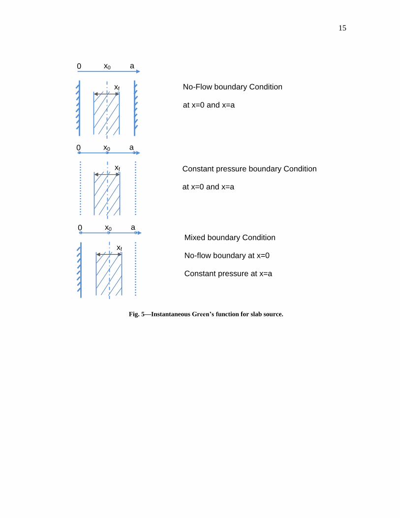
Fig. 5—Instantaneous Green’s function for slab source. ................................................. 15

Fig. 6—Slab source solution flowchart. ........................................................................... 17

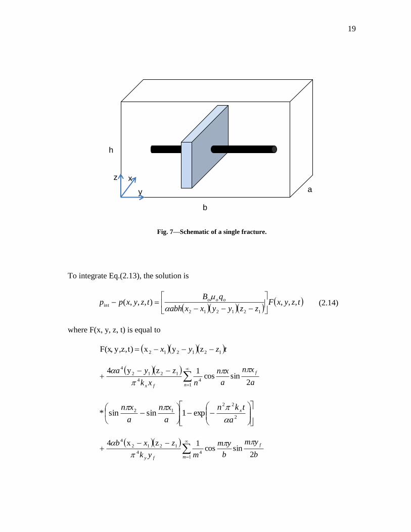
Fig. 7—Schematic of a single fracture. ............................................................................ 19

Fig. 8—Schematic of slab source for horizontal well. ..................................................... 28

Fig. 9—Discretized fracture. ............................................................................................ 29

Fig. 10—Segment fracture for finite conductivity. .......................................................... 32

Fig. 11—Flow chart for pressure drop inside fracture. .................................................... 36

Fig. 12—Transverse fractures along a horizontal well. ................................................... 38

Fig. 13—Transverse fractures with segments. ................................................................. 39

Fig. 14—Flow chart for Non-Darcy flow. ....................................................................... 46

Fig. 15—Schematic of complex fracture system. ............................................................ 47

Fig. 16—Comparison of the slab source model with Babu and Odeh’s model. .............. 52

Fig. 17—Comparison of the slab source model with Ouyang’s model. .......................... 53

Fig. 18— Comparison of the slab source model with DVS and simulation by Ecrin. .... 56

Fig. 19—Comparison of superposition procedure. .......................................................... 57

Fig. 20—Complex fracture system schematic. ................................................................ 58

x

Page

Fig. 21—ECLIPSE simulation results. ............................................................................ 60

Fig. 22—Slab source model results. ................................................................................. 60

Fig. 23—Set up for horizontal well. ................................................................................. 63

Fig. 24— Effect of wellbore length on production rate for kh=0.01md, kv=0.005md. .... 64

Fig. 25— Effect of wellbore length on production rate for kh=0.1md, kv=0.01md. ........ 64

Fig. 26—Effects of wellbore length on cumulative production (kh=0.01md). ................ 66

Fig. 27—Effects of wellbore length on cumulative production (kh=0.1md). .................. 66

Fig. 28—Percentage increases in cumulative production ................................................ 67

Fig. 29—Cases comparison for kh=0.1md and kv=0.01md. ............................................. 68

Fig. 30— Cases comparison for kh=0.01md and kv=0.001md. ........................................ 69

Fig. 31— Cases comparison for kh=0.001md and kv=0.0001md. .................................... 69

Fig. 32—Production increase ratio as a function of number of fractures. ....................... 71

Fig. 33—Fracture pressure profile for kh=0.1md, kv=0.01md, and kf=50000md. ........... 72

Fig. 34—Infinite conductivity vs. finite conductivity for kh=0.1md, kv=0.01md, and

kf=50000md. .................................................................................................... 73

Fig. 35—Flow rate profile for each fracture. ................................................................... 74

Fig. 36—Flow region for each fracture. ........................................................................... 74

Fig. 37— Randomly generated complex fracture system. ............................................... 76

Fig. 38—Flow rate for complex fracture system. ............................................................ 78

Fig. 39—Cumulative production for case 1. .................................................................... 79

Fig. 40—Cumulative production for Case 2. ................................................................... 80

xi

Page

Fig. 41—Cumulative production for Case 3. ................................................................... 81

Fig. 42—Field Data (Meyer and Bazan, 2010). ............................................................... 85

Fig. 43—History match of a gas well in Marcellus Shale. .............................................. 85

Fig. 44—Schematic of the formation. .............................................................................. 87

Fig. 45—Vertical well schematic. .................................................................................... 88

Fig. 46—Fractured vertical well schematic. .................................................................... 89

Fig. 47—Horizontal well schematic. ................................................................................ 89

Fig. 48—Slanted well with 82° and modified well for simulation. ................................. 90

Fig. 49—Cases comparison for production rate. .............................................................. 91

Fig. 50—Cases comparison for cumulative production. .................................................. 92

Fig. 51—Semi-infinite solid reservoir and slab source. ................................................. 104

Fig. 52—Finite solid bounded by the planes x=0 and x=a, slab source. ........................ 105

1

CHAPTER I

INTRODUCTION

1.1 Statement of the Problem

In recent years, hydrocarbon resources recoverable from reservoirs of different natures

have become important play. These resources are referred as “unconventional

resources”, including tight gas, gas/oil shale, oil sands, and coal-bed methane. North

America has a substantial growth in its unconventional oil and gas market over the last

two decades. The primary reason for that growth is because North America, being a

mature market, is beyond the peak production from its convention hydrocarbon

resources.

The defining characteristics of an unconventional resource are at best nebulous.

Etherington (2005) states “An unconventional reservoir is one that cannot be produced at

economic flow rates without assistance from massive stimulation treatments or special

recovery processes.” Others use a definition based upon two common aspects, they are

comprised of large volumes of rock pervasively charged with hydrocarbon, and that the

accumulation types are not dependent on buoyancy.

This dissertation follows the style of SPE Production & Operations.

2

New technology applications of multi-fractured horizontal wells allow us to produce

at economical rates from these low permeable oil and gas resources. Since commercial

exploration and production of oil and gas reservoirs began there have been

circumstances where the reservoir character or depositional model has caused difficulty

in assessment. Production assessment of unconventional reservoirs using standard

methodology has been notoriously problematic. The complexity of the fractured system

posts the challenges to analytical models, and reservoir simulation of such a system is

extremely time-consuming.

Although most of the solutions to the flow problem in porous media have been

investigated in a similar case as in the heat transfer and the solution is originated from

the heat transfer, Gringarten and Ramey’s (1973) work is the first application of the

Green’s and Source function to the problem of unsteady-state fluid flow in the

reservoirs. They introduced proper Green’s functions for a series of source shapes and

boundary conditions. They showed that the point source solution is actually a more

general theory of Green’s function, and used the integration of the response to an

instantaneous source solution to get the response for a continuous source solution. The

application of the Newman’s principle in breaking a problem of 3D into the product of

three 1 D solutions is also discussed in this work.

The application of source and Green’s function later extended to the unsteady-state

pressure distribution for more complex well completion schematics by others. The major

disadvantage of this method is the inherent singularity of the solution wherever the

source is placed. Since the source is assumed to have no volume (point, line source), the

3

source is considered to be at infinite pressure at the time zero and it is not possible to

calculate the exact pressure as a function of time at the point where source is placed. To

handle this problem, a source method with assigned volume needs to be developed.

Furthermore, as the petroleum industry goes toward producing lower quality reservoirs

like low- and ultra-low permeability reservoirs, the period of transient flow covers larger

part of the well lifetime and these pseudosteady-sate productivity calculations become

less applicable in prediction of the reservoir’s production behavior. A source method

needed to be able to fill this gap.

1.2 Objectives

In this proposed research, we present a different approach to the problem of unsteady

state flow of a compressible fluid in a rectilinear reservoir. The model is based on the

solution of a series of slab sources. It can be used to calculate well performance for

horizontal gas wells with or without fractures. Fractures can be longitudinal or

transverse, single or multiple, and fractures can be infinite conductivity or uniform

influx. Using the slab source approach, we assigned the sources (horizontal wells or

fractures) a geometry dimension and the effect of pressure behavior inside sources are

considered by superposition principles. This method is relatively easy to apply because

flow rate could be calculated directly from pressure difference between initial reservoir

4

pressure and pressure in fracture, which is the same as wellbore flow pressure for an

infinite conductivity fracture.

The research proposed in this project will develop a model to predict fractured

horizontal well performance in tight/shale gas reservoirs. It will accomplish the flowing

objectives.

1. To develop the slab source method as a solution to the problem of pressure and

production distribution in a closed, rectangular reservoir for a uniform flux

boundary condition.

2. To validate a series of solutions for pressure and flow rate behavior of simple and

complex well/fracture configurations such as:

Vertical well

Horizontal well

Multiple fractures along a horizontal well

Hydraulic fractured well with natural fractures

3. To demonstrate the applicability of the new solution method in predicting

pressure and production behavior for a complex well/fracture configuration.

4. To apply the new method as an optimization tool to obtain the best completion

schematic for development of an example case.

5. To study the flow effect inside of fractures by dividing the fracture into several

segments.

5

1.3 Literature Review

Over the past decades, point source integrated over a line and/or a surface has been

mostly used in solving single-phase flow problems in porous media when fluid

movement is from a complex fractured well system, Horizontal well models with point

source solution have been presented in many literatures.

Gringarten and Ramey (1973) were the first to apply the Green’s and source function

to the reservoir flow problems. They introduced Green’s function under different

boundary conditions for plane, slab, line, and point source. The source function is

combined with Newman’s product to de-component a problem in 3D to the product of

three 1D solutions.

Gringarten et al. (1974) applied the Green’s function later to the unsteady state

pressure distribution created by a vertical fractured well with infinite conductivity

fracture. By dividing the fracture into N segments, a series of equations had been solve

to calculate the pressure distribution and contribution of each segment to the total flow

by assuming each segment as a uniform flux source.

Cinco-Ley and Samaniego (1981) used the Green’s function under Laplace

transform to develop the model of finite conductivity vertical fracture in an infinite

reservoir. They presented a new technique for performing pressure transient analysis for

vertical finite-conductivity fractures using a bilinear flow model.

6

Point source solution was introduced by Ozkan et al. (1995). He developed point

source solution in Laplace domain in order to remove the limitations of the Gringarten

and Ramey’s model in considering the wellbore storage and skin effects.

By integrate the point source to line source, Babu and Odeh (1988) developed a line

source solution to predict horizontal well performance in a closed reservoir. The model

is under pseudosteady-state condition. One of the limitations of this method is the well

must be parallel to the reservoir boundary.

Goode and Kuchuk (1991) introduced solution for productivity of a horizontal well

in a reservoir with no-flow boundary and constant pressure boundary. Their solution is

expressed in the form of an infinite condition. A simplified solution for a short well was

developed in their study.

Ouyang et al. (1997) presented a 3D horizontal well model to describe wellbore

pressure and reservoir pressure change with time and location. The formula is in the

Laplace space. The transient pressure behaviors in physical space can be easily obtained

by means of the Stehfest algorithm.

Valko and Amini (2007) developed a method with distributed volume sources to

simulate fractured horizontal wells in a box-shaped reservoir. A source term was added

to the diffusivity equation to calculate the pressure distribution. Then the production rate

from a fracture is computed. Different from the other point source methods, the volume

source approach is able to describe the pressure behavior inside sources and its influence

to the flow field.

7

Zhu et al. (2007) showed applications of the volumetric source model and field cases

are presented in their work.

Meyer et al. (2010) presented a comprehensive methodology using the trilinear

solution to predicting the behavior of multiple transverse finite conductivity vertical

fractures in horizontal wellbores.

Miskimins et al. (2005) demonstrated that non-Darcy flow effects can influence well

productivity across the entire spectrum of flow rates, including low rates. They showed

that even in low velocity situations, non-Darcy effects can influence the productivity.

Non-Darcy flow can have a major impact on reduction of a propped half-length to a

considerably shorter effective half length, thus lowering the well’s productive capability

and overall reserve recovery.

8

CHAPTER II

METHODOLOGY

Point source and line source solutions have been used to solve petroleum engineering

problems in past years. The model is adapted from point source solutions of heat

conduction problem. The slab source solution of 3D problems is obtained by multiplying

three 1D slab sources together and integrating in time and along the source. This chapter

presents a semi-analytical slab source solution for 3D wellbore and fracture system in

this chapter. The model developed here can be applied to a variety of systems including

horizontal wells, slanted wells, single fracture, and multiply fractures along a horizontal

well. Firstly, the semi-analytical slab source solution is derived, and then the slab source

solution is applied to predict well performance for different well systems. It also

discusses the inner boundary conditions on the flow rate and wellbore pressure

distribution along the wellbore and fractures. Finally, the non-Darcy effect inside of the

fractures is studied.

2.1 Source Technique

The diffusivity equation of a single-phase incompressible fluid is written as Eq.(2.1)

t

p

k

c

x

p t

2

2

(2.1)

9

For an anisotropic medium, the diffusivity in three directional domains becomes

t

pc

z

pk

y

pk

x

pk tzyx

2

2

2

2

2

2

(2.2)

Because the diffusivity equation is in the same format as the heat conduction problems,

we can directly apply the sink/source technique to solve the flow in porous media.

2.1.1 Instantaneous Point Source

Gringarten and Ramey (1973) presented the instantaneous Green’s function in infinite

plane reservoir. The geometries of the source function are shown in Fig. 1 and Green’s

functions for different boundary conditions in infinite plane reservoirs are shown in

Table 1.

Table 1—Instantaneous Green’s function in 1D infinite reservoir.

Boundary Conditions Instantaneous Green’s functions for point source

Constant pressure

at x=0 and x=a

2

22

0

1

expsinsin2

a

kn

a

xn

a

xn

a

x

n

No-Flow

at x=0 and x=a

2

22

0

1

expcoscos211

a

kn

a

xn

a

xn

a

x

n

No-Flow at x=0

Constant pressure

at x=0

2

22

0

1 4

12exp

12cos

12cos

2

a

kn

a

xn

a

xn

a

x

n

where, tc .

10

Fig. 1—Instantaneous Green’s function for point source.

For a 3D problem Newman’s product can be applied to instantaneous Green’s and

source functions which solves a 3D problem by multiplication of three 1D problem

solution. The instantaneous Green’s function for a 3D reservoir that can be visualized as

the intersection of three one-dimensional reservoirs is equal to the product of the

instantaneous Green’s function for each one-dimensional reservoir. For example, the

x=0 x=a

No-flow boundary condition

at x=0 and x=a

x=0 x=a

Constant pressure boundary condition

at x=0 and x=a

x=0 x=a Mixed boundary condition

No-flow boundary at x=0

Constant pressure at x=a

11

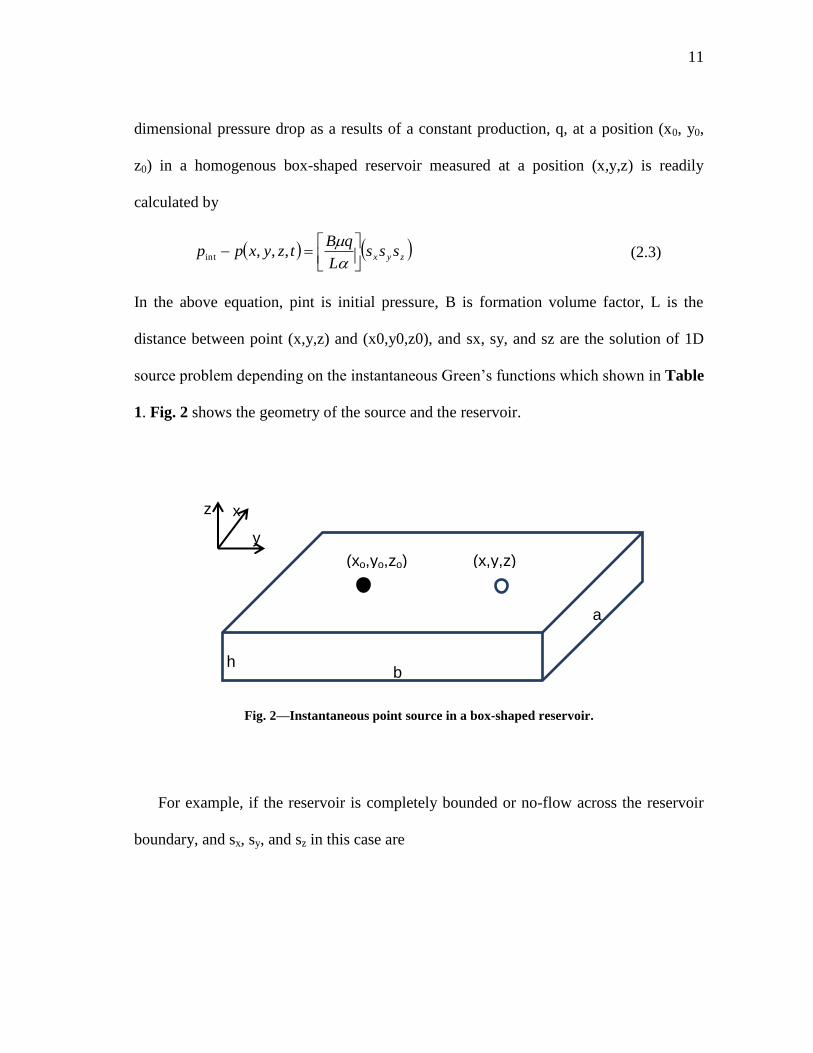
dimensional pressure drop as a results of a constant production, q, at a position (x0, y0,

z0) in a homogenous box-shaped reservoir measured at a position (x,y,z) is readily

calculated by

zyx sssL

qBtzyxpp

,,,int (2.3)

In the above equation, pint is initial pressure, B is formation volume factor, L is the

distance between point (x,y,z) and (x0,y0,z0), and sx, sy, and sz are the solution of 1D

source problem depending on the instantaneous Green’s functions which shown in Table

1. Fig. 2 shows the geometry of the source and the reservoir.

Fig. 2—Instantaneous point source in a box-shaped reservoir.

For example, if the reservoir is completely bounded or no-flow across the reservoir

boundary, and sx, sy, and sz in this case are

(xo,yo,zo) (x,y,z)

h b

a

z

y

x

12

2

22

0

1

expcoscos211

a

kn

a

xn

a

xn

as x

n

x

(2.4)

2

22

0

1

expcoscos211

b

km

b

yn

b

yn

bs

y

m

y

(2.5)

2

22

0

1

expcoscos211

h

kl

h

zn

h

zn

hs z

l

z

(2.6)

2.1.2 Continuous Point Source Solution

By integrating the continuous point source solution along a line, the continuous line

source solution could be developed. For a line source that have the initial position at (x01,

y01, z01) and the end point at (x02, y02, z02) as shown in Fig. 3, the solution of the

continuous line source in dimensional format can be written as,

dydsssL

qBtzyxpp

y

y

t

zyx

2

1 0

000

int ,,, (2.7)

The sx, sy, and sz can be any combinations of the instantaneous Green’s function

depending on the boundary conditions in Table 1.

13

Fig. 3—Schematic of a horizontal well trajectory in line source.

2.1.3 Slab Source Solution

The slab source method solves the flow problem in a parallelepiped porous medium with

a slab source, s, placed in the domain, as shown in Fig. 4. The reservoir is assumed to be

an anisotropic porous medium. Following the same approach as the conventional point

source solution to apply Newman’s principle, the three-dimensional pressure response of

the system to an instantaneous source can be obtained as the production of the solutions

of three one-dimensional problems from each principal direction.

z

y

x

(xo,yo1,zo1) (xo,yo2,zo2)

h b

a

14

Fig. 4—Schematic of the slab source model.

The solution from this technique applies to different state in the flow period, both

transient flow and stabilized flow. The boundary condition of the reservoir can be

constant pressure boundary, no-flow boundary or mixed boundary, which makes the

model practical to a wide range of flow problems in petroleum engineering.

The procedure of obtaining the solution is to obtain one-dimensional solution of the

slab problem, applying Newman’s product method based on instantaneous source

function in an infinite reservoir to get three-dimensional solution, and then integrates the

three-dimensional solution over time to get a continuous source function. Modifying the

point source domain by placing a pair of parallel plates in the domain, as shown in Fig.

5, we began the model with one-dimensional instantaneous infinite slab source in an

infinite slab reservoir. Green’s functions (Carslaw and Jaeger, 1959) for different

boundary conditions in infinite slab domain with a system schematic are shown in Table

2.

z

y

x

s

b

a

h

15

Fig. 5—Instantaneous Green’s function for slab source.

No-Flow boundary Condition

at x=0 and x=a

0

0

x0 a

xf

Constant pressure boundary Condition

at x=0 and x=a

xf

0

0

x0 a

Mixed boundary Condition

No-flow boundary at x=0


xf

0

0

x0 a

16

Table 2—Instantaneous Green’s function in 1D infinite slab reservoir (Carslaw and Jaeger, 1959).

Boundary Conditions Instantaneous Green’s Functions

Constant pressure

at x=0 and x=a

12

22

expsinsin2

sin14

n

xof

a

kn

a

xn

a

xn

a

xn

n

No-flow

at x=0 and x=a

2

22

1

coscos2

sin14

1a

knxpe

a

xn

a

xn

a

xn

nx

a

a

xx

n

of

f

f

No-flow at x=0


1

12cos

12cos

4

12sin

12

18

n

of

a

xn

a

xn

a

xn

n

2

22

4

12exp

a

kn x

Staring with an instantaneous slab source in an infinite one-dimensional reservoir

(Fig. 5), overlaying three of such sources in x, y, and z direction makes a three-

dimensional instantaneous slab source in a box-shaped reservoir. To obtain the solution

of the new system, we multiple the three solutions of the original one-dimensional

problem to have an instantaneous solution for the three-dimensional system. Integrate

over the well trajectory or the fracture length and height to get the instantaneous slab

source solution for the performance of the well, and then integrate over the time to get

the three-dimension continuous slab source solution to solve practical reservoir

problems. The procedure is summarized in Fig. 6. The solution as instantaneous source

depends on the locations of the slab source and the box shape reservoir. To apply this

method for horizontal wells with or without fractures, we define the source term (the

17

location and the dimensions of the source) and the main domain according to each

individual physical system.

Fig. 6—Slab source solution flowchart.

For instance, the pressure drop as a results of a constant production, q, at a position

(x0,y0,z0) in an anisotropic box-shaped reservoir measured at a position (x, y, z) is

readily calculate by

zyx sssabh

qBtzyxpp

,,,int (2.8)

Instantaneous

Green’s function in

1D infinite reservoir

Instantaneous Slab

source in 3D

Continuous Slab

source in 3D

Fracture solution

Newman’s product

In x, y, z direction

Integrate over time

Integrate over Fracture

18

where, a is reservoir width, b is reservoir length, h is reservoir height, and sx, sy and sz

are the slab source functions in each direction depending on the boundary conditions, as

shown in Table 2.

For no-flow boundary condition, and sx, sy, and sz are

2

22

1

coscos2

sin14

1a

knxpe

a

xn

a

xn

a

xn

nx

a

a

xs x

n

of

f

f

x

(2.9)

2

22

1

coscos2

sin14

1b

kmxpe

b

ym

b

ym

b

ym

my

b

b

ys

y

m

of

f

f

y

(2.10)

2

22

1

coscos2

sin14

1h

klxpe

h

zl

h

zl

h

zl

lz

h

b

zs z

l

of

f

f

z

(2.11)

After obtain the instantaneous slab source solution under defined boundary

conditions, we integrate the instantaneous point source over a time interval to attain the

continuous slab source solution. The pressure drop at point (x, y, z) as a result of the

continuous production or injection at position (x0, y0, z0) in an anisotropic box-shaped

reservoir then is

dsss

abh

qBtzyxpp

t

zyx

0

000

int ,,, (2.12)

For the slab source representing a fracture as shown in Fig. 7, the solution of the

continuous slab source can be written as,

dxdydzdsssabh

qBtzyxpp

z

z

y

y

x

x

t

zyx

2

1

2

1

2

1 0

000

int ,,, (2.13)

19

Fig. 7—Schematic of a single fracture.

To integrate Eq.(2.13), the solution is

tzyxFzzyyxxabh

qBtzyxpp ooo ,,,),,,(

121212

int

(2.14)

where F(x, y, z, t) is equal to

tzyx 121212 zyxt)z,y,F(x,

a

xn

a

xn

nxk

zya f

nfx2

sincos1zy4

144

1212

4

2

22

12 exp1sinsin*a

tkn

a

xn

a

xn x

b

ym

b

ym

myk

zxb f

mfy2

sincos1zx4

144

1212

4

b

a

h

z

y

x

20

2

22

12 exp1sinsin*b

tkm

b

ym

b

ym x

h

zn

h

zl

lzk

yxh f

lfz2

sincos1yx4

144

1212

4

2

22

12 exp1sinsin*h

tkl

h

zl

h

zl z

b

ym

b

ym

a

xn

a

xn

yx

zba

m nff

12

1 1

12

6

12

22

sinsinsinsinz16

2

2

2

22

2

2

2

222

2

exp1

sin2

sincos2

sin

*b

km

a

knt

b

km

a

knmn

b

xm

b

ym

a

xn

a

xn

yx

yx

f

h

zl

h

zl

a

xn

a

xn

zx

yha

n lff

12

1 1

12

6

12

22

sinsinsinsiny16

2

2

2

22

2

2

2

222

2

exp1

sin2

sincos2

sin

*h

kl

a

knt

h

kl

a

knln

h

zl

h

zl

a

xn

a

xn

zx

zx

f

h

zl

h

zl

b

ym

b

ym

zy

xhb

m lff

12

1 1

12

6

12

22

sinsinsinsinx16

2

2

2

22

2

2

2

2

22

2

exp1

sin2

sincos2

sin

*h

kl

b

kmt

h

kl

b

kmlm

h

zl

h

zl

b

ym

b

ym

zy

zy

f

1 1 1

1212

8

222

sinsinsinsin64

n m lfffb

ym

b

ym

a

xn

a

xn

zyx

hba

21

2

2

2

2

2

22

12 exp1sinsin*h

kl

b

km

a

knt

h

zl

h

zl zyx

2

2

2

2

2

2222

2 sin2

sincos2

sincos2

sin

*

h

kl

b

km

a

knlmn

h

zl

h

zl

b

ym

b

ym

a

zn

a

xn

zyx

ff

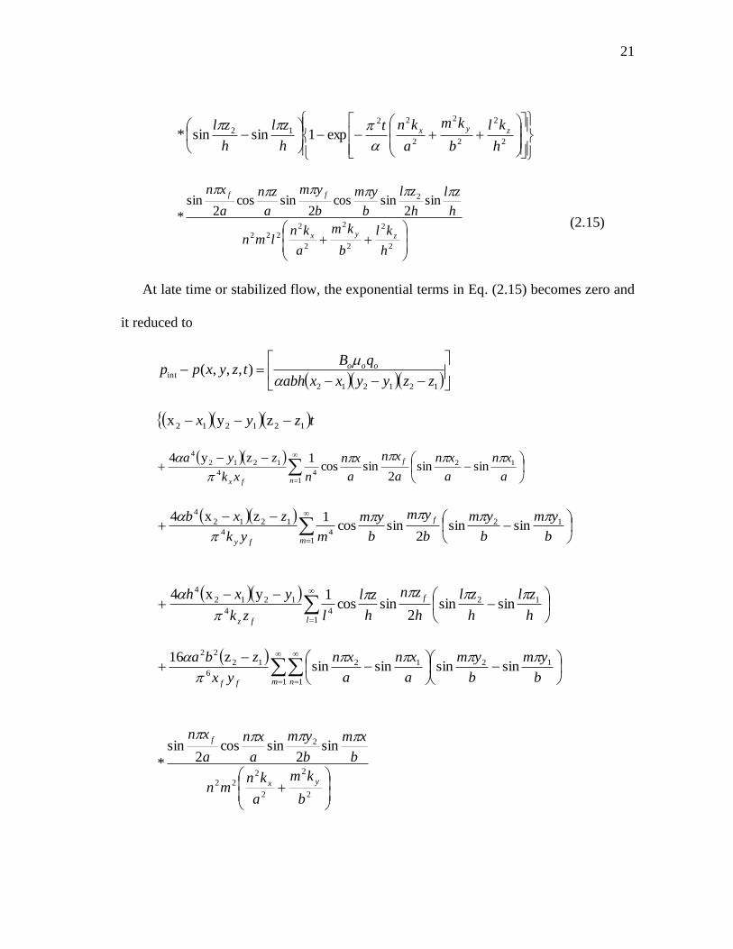
(2.15)

At late time or stabilized flow, the exponential terms in Eq. (2.15) becomes zero and

it reduced to

121212

int ),,,(zzyyxxabh

qBtzyxpp ooo

tzyx 121212 zyx

a

xn

a

xn

a

xn

a

xn

nxk

zya f

nfx

12

144

1212

4

sinsin2

sincos1zy4

b

ym

b

ym

b

ym

b

ym

myk

zxb f

mfy

12

144

1212

4

sinsin2

sincos1zx4

h

zl

h

zl

h

zn

h

zl

lzk

yxh f

lfz

12

144

1212

4

sinsin2

sincos1yx4

b

ym

b

ym

a

xn

a

xn

yx

zba

m nff

12

1 1

12

6

12

22

sinsinsinsinz16

2

2

2

222

2 sin2

sincos2

sin

*

b

km

a

knmn

b

xm

b

ym

a

xn

a

xn

yx

f

22

h

zl

h

zl

a

xn

a

xn

zx

yha

n lff

12

1 1

12

6

12

22

sinsinsinsiny16

2

2

2

222

2 sin2

sincos2

sin

*

h

kl

a

knln

h

zl

h

zl

a

xn

a

xn

zx

f

h

zl

h

zl

b

ym

b

ym

zy

xhb

m lff

12

1 1

12

6

12

22

sinsinsinsinx16

2

2

2

2

22

2 sin2

sincos2

sin

*

h

kl

b

kmlm

h

zl

h

zl

b

ym

b

ym

zy

f

1 1 1

1212

8

222

sinsinsinsin64

n m lfffb

ym

b

ym

a

xn

a

xn

zyx

hba

2

2

2

2

2

2

222

2

12

sin2

sincos2

sincos2

sin

sinsin*

h

kl

b

km

a

knlmn

h

zl

h

zl

b

ym

b

ym

a

zn

a

xn

h

zl

h

zl

zyx

ff

(2.16)

For stabilized flow under pseudo-steady-state condition, the average reservoir

pressure can be written as

tp

po

cV

NBpp int (2.17)

Defining the drainage volume, then

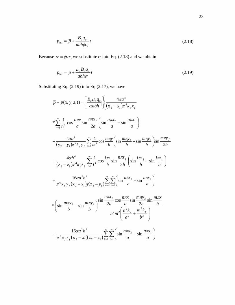
23

tcabh

qBpp

t

oo

int (2.18)

Because tc we substitute into Eq. (2.18) and we obtain

tabh

qBpp ooo

int (2.19)

Substituting Eq. (2.19) into Eq.(2.17), we have

fx

ooo

xkx

a

abh

qBtzyxpp

4

12

4

x

4),,,(

a

xn

a

xn

a

xn

a

xn

n

f

n

12

14

sinsin2

sincos1

*

b

ym

b

ym

b

ym

b

ym

myky

b f

mfy2

sinsinsincos1

y

4 12

144

12

4

h

zl

h

zl

h

zn

h

zl

lzkz

h f

lfz

12

144

12

4

sinsin2

sincos1

z

4

1 1

12

1212

6

22

sinsinzx

16

m nffa

xn

a

xn

yyxyx

ba

*

2

2

2

222

2

12

sin2

sincos2

sin

sinsin

b

km

a

knmn

b

xm

b

ym

a

xn

a

xn

b

ym

b

ym

yx

f

1 1

12

1212

6

22

sinsinzx

16

n lffa

xn

a

xn

zxzx

ha

24

2

2

2

222

2

12

sin2

sincos2

sin

sinsin*

h

kl

a

knln

h

zl

h

zl

a

xn

a

xn

h

zl

h

zl

zx

f

1 1

12

1212

6

22

sinsinzy

16

m lffb

ym

b

ym

zyzy

hb

2

2

2

2

22

2

12

sin2

sincos2

sin

sinsin*

h

kl

b

kmlm

h

zl

h

zl

b

ym

b

ym

h

zl

h

zl

zy

f

1 1 1

12

121212

8

222

sinsinzyx

64

n m lfffa

xn

a

xn

zyxzyx

hba

h

zl

h

zl

b

ym

b

ym 1212 sinsinsinsin*

2

2

2

2

2

2222

2 sin2

sincos2

sincos2

sin

*

h

kl

b

km

a

knlmn

h

zl

h

zl

b

ym

b

ym

a

zn

a

xn

zyx

ff

(2.20)

In oil field unit, Eq. (2.20) becomes

fx

ooo

xkx

a

abh

qBtzyxpp

4

12

4

x

453.887),,,(

a

xn

a

xn

a

xn

a

xn

n

f

n

12

14

sinsin2

sincos1

*

25

b

ym

b

ym

b

ym

b

ym

myky

b f

mfy2

sinsinsincos1

y

4 12

144

12

4

h

zl

h

zl

h

zn

h

zl

lzkz

h f

lfz

12

144

12

4

sinsin2

sincos1

z

4

1 1

12

1212

6

22

sinsinzx

16

m nffa

xn

a

xn

yyxyx

ba

2

2

2

222

2

12

sin2

sincos2

sin

sinsin*

b

km

a

knmn

b

xm

b

ym

a

xn

a

xn

b

ym

b

ym

yx

f

1 1

12

1212

6

22

sinsinzx

16

n lffa

xn

a

xn

zxzx

ha

2

2

2

222

2

12

sin2

sincos2

sin

sinsin*

h

kl

a

knln

h

zl

h

zl

a

xn

a

xn

h

zl

h

zl

zx

f

1 1

12

1212

6

22

sinsinzy

16

m lffb

ym

b

ym

zyzy

hb

2

2

2

2

22

2

12

sin2

sincos2

sin

sinsin*

h

kl

b

kmlm

h

zl

h

zl

b

ym

b

ym

h

zl

h

zl

zy

f

121212

8

222

zyx

64

zyxzyx

hba

fff

26

2

2

2

2

2

2222

2 sin2

sincos2

sincos2

sin

h

kl

b

km

a

knlmn

h

zl

h

zl

b

ym

b

ym

a

zn

a

xn

zyx

ff

(2.21)

where tc 73.158

For gas reservoir, Eq.(2.20) becomes

fx

o

xkx

a

abh

ZTqtzyxpp

4

12

422

x

48947),,,(

a

xn

a

xn

a

xn

a

xn

n

f

n

12

14

sinsin2

sincos1

*

b

ym

b

ym

b

ym

b

ym

myky

b f

mfy2

sinsinsincos1

y

4 12

144

12

4

h

zl

h

zl

h

zn

h

zl

lzkz

h f

lfz

12

144

12

4

sinsin2

sincos1

z

4

1 1

12

1212

6

22

sinsinzx

16

m nffa

xn

a

xn

yyxyx

ba

2

2

2

222

2

12

sin2

sincos2

sin

sinsin*

b

km

a

knmn

b

xm

b

ym

a

xn

a

xn

b

ym

b

ym

yx

f

1 1

12

1212

6

22

sinsinzx

16

n lffa

xn

a

xn

zxzx

ha

27

2

2

2

222

2

12

sin2

sincos2

sin

sinsin*

h

kl

a

knln

h

zl

h

zl

a

xn

a

xn

h

zl

h

zl

zx

f

1 1

12

1212

6

22

sinsinzy

16

m lffb

ym

b

ym

zyzy

hb

2

2

2

2

22

2

12

sin2

sincos2

sin

sinsin*

h

kl

b

kmlm

h

zl

h

zl

b

ym

b

ym

h

zl

h

zl

zy

f

1 1 1

12

121212

8

222

sinsinzyx

64

n m lfffa

xn

a

xn

zyxzyx

hba

h

zl

h

zl

b

ym

b

ym 1212 sinsinsinsin

2

2

2

2

2

2222

2 sin2

sincos2

sincos2

sin

h

kl

b

km

a

knlmn

h

zl

h

zl

b

ym

b

ym

a

zn

a

xn

zyx

ff

(2.22)

2.1.4 Horizontal Well in Slab Source Solution

Using the slab source solution to calculate a horizontal well without fractures

performance, first define inner boundary condition, then to count pressure change inside

a wellbore, we divide the wellbore into N segments. Each segment connects to each

other by superpositioning in space. By using this technique, a set of linear equation is

28

generated and the solution of the system equation predicts the well performance. For

horizontal well showed in Fig. 8, the pressure drop causes by a constant production flow

rate, q1, into segment 1 is evaluated on the well circumstance are the middle of every

well segment. For each segment, we have a set of N linear equations for pressure

respond to the flow. With N segments, there are N set of N linear equations as shown in

Eq. (2.24).

Fig. 8—Schematic of slab source for horizontal well.

1321 ),1(...)3,1()2,1()1,1( pNFqFqFqFq N

2321 ),2(...)3,2()2,2()1,2( pNFqFqFqFq N

3321 ),3(...)3,3()2,3()1,3( pNFqFqFqFq N

.

.

.

b

a

h

1 2 N N-1

29

NN pNNFqNFqNFqNFq ),(...)3,()2,()1,( 321 (2.23)

2.1.5 Fracture System in Slab Source Solution

For fractures, we divided each fracture into N*N segments, each segment will create

flow rate from the reservoir. For example, we have a fracture with 25 segments as shown

in Fig. 9, each segment is contact with each other. To simplify the problem, it is

assumed that in such a system, only fracture create flow rate. Similar to the horizontal

well system, each segment will generate flow rate from the reservoir. Because of the

flow rate in the segment 1, the pressure for the other 24 segment will be changed. By the

same way, the flow rate of the second segment would change the pressure distribution in

the other 24 segments. With N*N segments, we have a set of N*N linear equations for

pressure respond to the flow in the fracture. The horizontal well takes flow rate from the

fracture, but not directly from the reservoir.

Fig. 9—Discretized fracture.

hf

2xf

1 N

N

2

30

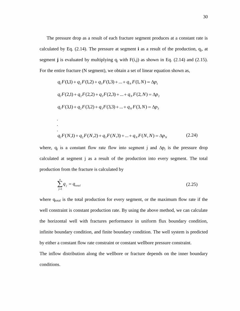
The pressure drop as a result of each fracture segment produces at a constant rate is

calculated by Eq. (2.14). The pressure at segment i as a result of the production, qj, at

segment j is evaluated by multiplying qj with F(i,j) as shown in Eq. (2.14) and (2.15).

For the entire fracture (N segment), we obtain a set of linear equation shown as,

1321 ),1(...)3,1()2,1()1,1( pNFqFqFqFq N

2321 ),2(...)3,2()2,2()1,2( pNFqFqFqFq N

3321 ),3(...)3,3()2,3()1,3( pNFqFqFqFq N

.

.

.

NN pNNFqNFqNFqNFq ),(...)3,()2,()1,( 321 (2.24)

where, qj is a constant flow rate flow into segment j and ∆pj is the pressure drop

calculated at segment j as a result of the production into every segment. The total

production from the fracture is calculated by

total

n

j

j qq 1

(2.25)

where qtotal is the total production for every segment, or the maximum flow rate if the

well constraint is constant production rate. By using the above method, we can calculate

the horizontal well with fractures performance in uniform flux boundary condition,

infinite boundary condition, and finite boundary condition. The well system is predicted

by either a constant flow rate constraint or constant wellbore pressure constraint.

The inflow distribution along the wellbore or fracture depends on the inner boundary

conditions.

31

2.1.6 Solution for Infinite Conductivity Condition

In infinite conductivity condition for fractures, we divided the source into N segments.

For a source under infinite conductivity, uniform pressure over the source is assumed.

Fig. 9 shows an example of how the source is discretized into 25 segments. For the

infinite conductivity inner boundary condition, the wellbore pressure is constant along

the well or the fracture. The right hand side in Eq. (2.26) have the same pressure drop

which shown in Eq. (2.27).In this way, we could solve the set of liner equations and get

the flow rate along the fracture.

125321 )25,1(...)3,1()2,1()1,1( ppFqFqFqFq i

225321 )25,2(...)3,2()2,2()1,2( ppFqFqFqFq i

325321 )25,3(...)3,3()2,3()1,3( ppFqFqFqFq i

.

.

.

2525321 )25,25(...)3,25()2,25()1,25( ppFqFqFqFq i (2.26)

252 ... pppi (2.27)

2.1.7 Solution for Finite Conductivity Condition

For the cases with finite conductivity we use the same approach as the infinite

conductivity except we have to introduce another term to account for the pressure drop

between source segments because of the source conductivity.

32

We first define the inner boundary condition at the interface of the source and the

domain (for example, the wellbore and the reservoir). Then we divide the fracture into

multiple segments. The segments are then connected to each other by super position in

the space. By using this technique, a set of linear equation is generated and solved to

predict the fractured horizontal well performance. Fig. 10 shows an example for 25

sources fracture. We first allow source 1 to exist in the reservoir and let it generate a

flow rate of q1 at the location. The flow results in corresponding pressure changes at

locations of sources 2 through 25. Then if we only let source 2 exists the pressure also

changes at all source locations. We can apply this procedure to all 25 sources in the

system. To illustrate the influence of the source location, we use dimensional format of

the equations in this section.

Fig. 10—Segment fracture for finite conductivity.

An additional pressure drop will be added to the calculation, which is showed in Fig.

10. Three circles are defined in the fracture. Circle 1 is in blue, circle 2 is in green and

hf

2xf

Circle 1

Circle 2

Circle 3

w

hf

2xf

1 5 2 4 3

11 15 12 14 8

16 20 17 19 18

6 10 7 9 8

21 25 22 24 23

33

circle 3 is in pink. The fluid will firstly flow from the out boundary to inner boundary of

circle 1(seg. 1-5, 6, 10-11, 15-16, and 20-25). Then the fluid flows inside circle 2(seg. 7-

9, 12, 14, 17-19). Finally it flows from circle 3 to wellbore. In such a way, we could

easily calculate the pressure drop inside of the fracture by Eq. (2.28).

qsrC

A

kh

Bpp

wA

wf

2

4ln

2

12.141

(2.28)

where, A is drainage area, CA is shape facture, and is Euler’s constant.

The Earlougher’s shape factor is shown in Table 3.

Table 3—Shape factor (Earlougher, 1977).

Drainage Area Earlougher Shaper Factor

30.9

21.8

5.38

2.36

1

5

1

4

2

1

34

The procedures for calculating the flow rate and pressure drop along the fractures

have two parts. One is from the reservoir to the fracture. The other is inside of the

fractures. An example used here for a transverse fracture with 25 segments.

First it is the reservoir to fracture system. The fracture is divided into 25 segments.

We start from the first segment to the last segment. The segment 1 will generate the flow

rate from the reservoir, q1, flowing into the fracture by using Eq. (2.22). After this

calculation, we will have 25 F(1, j) terms. Then we move to the next segment which is

segment 2 and repeat the same procedure but for this segment we evaluate the pressure

drop as a result of a constant flow, q2, flowing into segment 2 which gives another 25

F(2, j). We use the superposition principle in space to get a set of linear equation. The

series of linear equation can be written as Eq. (2.29)

25

3

2

1

)25,25()2,25()1,25(

)25,3()2,3()1,3(

)25,2()2,2()1,2(

)25,1()2,1()1,1(

25

3

2

1

int

int

int

int

.

.

.

...,

.

.

.

...,

...,

...,

.

.

.

.

.

.

q

q

q

q

FFF

FFF

FFF

FFF

p

p

p

p

p

p

p

p

(2.29)

Then, fluid inside fracture is analyzed. As shown in Fig. 10, for circle 1, the pressure

drop in these segments could be calculated by Eq. (2.28). We rewrite the equation as the

following

11,1, circlecircleinnercirclei Bqpp (2.30)

pi is the pressure at the middle point of each segment.

35

In the circle 2, the fluid flows from the out boundary of circle 2 to the middle of the

segment, then to the inner boundary of circle 2. The flow rate will be the fluid flow

inside of the segment plus the fluid comes from the circle 1.

22,2, circlecircleinnerciclei Cqpp (2.31)

22,2, circlecircleicirlceout Eqpp (2.32)

Finally the fluid flows inside circle 3 from out boundary of circle 3 to the wellbore, it

could be written as

33, circlewfcircleout Dqpp (2.33)

where, pwf is the wellbore pressure.

To solve these equations, subsisting Eqs. (2.30), (2.31), Eq. (2.33) into Eq. (2.29)

yields

icircleoutcircleinnercircleinner qDCBApppp 3,2,1,int (2.34)

Adding Eq. (2.31) and Eq. (2.32)

icircleinnercircleout qCEpp 2,2, (2.35)

where B, C, D, and E are the left part of Eq.(2.18) with different rw, CA, and A.

We also set that

2,3, circleinnercircleout pp (2.36)

and

1,2, circleinnercircleout pp (2.37)

36

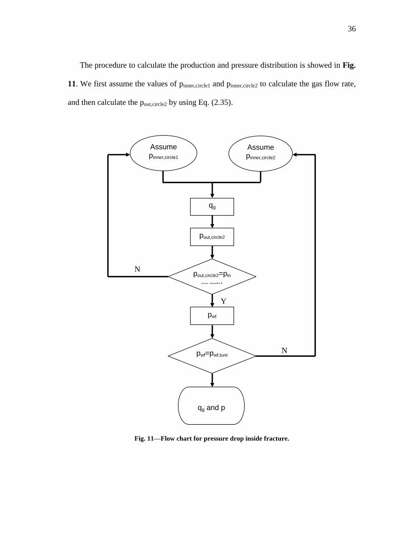
The procedure to calculate the production and pressure distribution is showed in Fig.

11. We first assume the values of pinner,circle1 and pinner,circle2 to calculate the gas flow rate,

and then calculate the pout,circle2 by using Eq. (2.35).

Fig. 11—Flow chart for pressure drop inside fracture.

qg

pout,circle2

pout,circle2=pin

ner,circle1

N

pwf

Y

pwf=pwf,ture N

Assume pinner,circle1

Assume pinner,circle2

qg and p

37

We compared the pout,circle2 and pinner,circle1 to check whether they are the same. If it is

not, we will set a new pinner,circle1 value which is equal to pout,2 to iterate until pout,cirlce2 is

equal to pinner,circle1. Then we will move to the next step to calculate pwf using Eq. (2.33).

Comparing with the true pwf which is a given parameter, if they are same then we

calculate the flow rate and pressure distribution in the fracture. If it is not, then we

increase or decrease the pinner,circle2 value to iterate again until the pwf is converged.

2.1.8 Solution for Multi-Fractures System

A schematic of transverse fractures with a horizontal well is illustrated in Fig.12. As a

simple example, we consider a two-transverse-fracture. For transverse fractures

intercepting a horizontal well, the fractures are represented as infinitely conductive or

with uniform flux under the assumption that the fractures are dominating the total

production to the well. Each fracture can be treated as an individual source and their

effects to other fractures are included through the superposed pressure drawdown.

38

Fig. 12—Transverse fractures along a horizontal well.

Eq. (2.22) can be directly used in this case. In the equation i denotes the location that

observes the pressure change, and j denotes the fracture that causes the pressure change.

If considering pressure drop in the wellbore between fractures, then

iwellboreiwfiwf ppp ,1,, (2.38)

To calculate the well performance, we first place fracture 1 in the system, which

causes a flow rate of q1 at the location of the fracture 1. The flow results in

corresponding pressure changes at both locations of the fracture 1 and the fracture 2.

Then if assume only fracture 2 exist, the pressure also changes at both locations. Since

the total pressure drawdown at each fracture should be the sum of the pressure drops

caused by all the fractures in the system, by the superposition principle, we have

1),,,(int *),,,(1

qtzyxFpp tzyx

2),,,(int *),,,(2

qtzyxFpp tzyx (2.39)

Fracture 2

Fracture 1 Wellbore

39

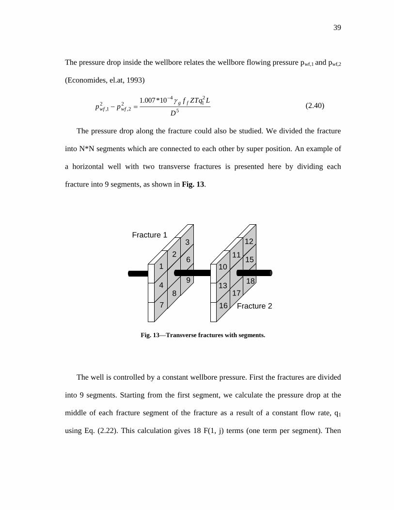
The pressure drop inside the wellbore relates the wellbore flowing pressure pwf,1 and pwf,2

(Economides, el.at, 1993)

5

21

4

22,

21,

10*007.1

D

LZTqfpp

fg

wfwf

(2.40)

The pressure drop along the fracture could also be studied. We divided the fracture

into N*N segments which are connected to each other by super position. An example of

a horizontal well with two transverse fractures is presented here by dividing each

fracture into 9 segments, as shown in Fig. 13.

Fig. 13—Transverse fractures with segments.

The well is controlled by a constant wellbore pressure. First the fractures are divided

into 9 segments. Starting from the first segment, we calculate the pressure drop at the

middle of each fracture segment of the fracture as a result of a constant flow rate, q1

using Eq. (2.22). This calculation gives 18 F(1, j) terms (one term per segment). Then

Fracture 1

Fracture 2

1

2

3

4

6

7

8

9

10

11

12

13

15

16

17

18

40

we move to the next segment (segment 2) and repeat the same procedure but for this

segment we evaluate the pressure drop as a result of constant flow, q2, flowing into

segment 2 which gives another 18 F(2, j). We continue this calculation to the last

segment. At this point we will obtain totally 18*18 F(i, j) terms. Then we use the

superposition principle in space to connect the wellbore segments. This yields a set of

linear equations.

1int18321 )18,1(...)3,1()2,1()1,1( ppFqFqFqFq

2int18321 )18,2(...)3,2()2,2()1,2( ppFqFqFqFq

3int18321 )18,3(...)3,3()2,3()1,3( ppFqFqFqFq

.

.

.

18int321 )18,18(...)3,18()2,18()1,18( ppFqFqFqFq N (2.41)

The series of linear equation can be written as Eq. (2.41). Then we solve this linear

system by defining the inner boundary condition.

The matrix solver used here already encountered the inverses of matrices if it is

nonsingular. Gauss-Jordan elimination is used to determine whether a given matrix is

invertible and find the inverse. Gauss-Jordan elimination is an algorithm for getting

matrices in reduced row echelon form using elementary row operations. It is a variation

of Gaussian elimination. Gaussian elimination places zeros below each pivot in the

matrix, starting with the top row and working downwards. Matrices containing zeros

below each pivot are said to be in row echelon form. Gauss-Jordan elimination goes a

41

step further by placing zeros above and below each pivot; such matrices are sid to be in

reduced row echelon form. Every matrix has a reduced row echelon form, and Gauss-

Jordan elimination is guaranteed to find it.

If Gauss-Jordan elimination is applied on a square matrix, it can be used to calculate

the matrix’s inverse. This can be done by augmenting the square matrix with the identity

matrix of the same dimensions and applying the following matrix operation.

11 IAAIAAI (2.42)

2.1.9 Non-Darcy Flow

The existence of non-Darcy effects in the flow of fluids through porous media has been

studied by petroleum industry for many years; however, characterizing and assessing in

magnitude of these effects is still proved difficult.

Henry Darcy developed flow correlation through sand pack configurations in 1856

by flowing water at the local hospital. His results are based on a series of experiments on

water flow through a sand packed column at various pressure differentials. From these

various experiments he concluded that flow rate varied in proportion to the imposed

head and inversely to the height of the sand pack. Darcy’s law describes that the linear

proportionality which is in Eq. (2.43) involving a constant, k, is related to the potential

gradient ∂p/∂L, the fluid viscosity of µ, and the superficial velocity of v.

42

kL

p

(2.43)

In 1901, Forchheimer Observed that the deviation from linearity in Darcy’s law

increased with flow rate. He proposed a second proportionality constant to describe the

increasing pressure drop caused by inertial losses. He assumes that Darcy’s Law is still

valid, but added an additional pressure drop. The familiar Forchheimer equation is

shown in Eq. (2.44)

2

fkL

p (2.44)

When the flow velocity is low, the second term in Eq. (2.44) can be neglected. However,

for higher velocities this term becomes more important, especially for low viscosity

fluids. If dividing Eqs.(2.43) and (2.44) by g we obtain

fkL

p 1

(2.45)

for Darcy flow and

21

fkvL

p (2.46)

for non-Darcy flow. Comparing Eq. (2.45) and (2.46) we see that the effective

permeability (determining the actual pressure drop) is

f

f

efffk

kk

1

(2.47)

43

The second term in the denominator of the right-hand side is dimensionless and acts as a

Reynolds Number for porous media flow. The Reynolds number in a porous media can

be defined as

fkN Re (2.48)

where, kf is in Darcy or cm-g/100sec2-atm, is in g/cm

3, is in cm/s, ug is in cp or

g/100cm-sec and is in atm-sec2/gm.

Suggested by Geertsma (1974) , substituting Eq. (2.48) into Eq. (2.47), the final

expression of kf-eff describing the non-Darcy flow effects is

Re1 N

kk

f

efff

(2.49)

where velocity in Eq.(2.48)

A

q353.0 (2.50)

where, q is in Mscf/day and A is in ft2.

In hydraulic fracturing operations, the non-Darcy flow effect has been addressed by

Cooke (1973). The oil industry attempts to study the impact of non-Darcy effects under

different producing situations in the past several years. Non-Darcy effects can

significantly decrease well production especially in high flow rate well. Smith, et al

(2004), claimed that non-Darcy flow effects decrease 35% in productivity in a

hydraulically fractured high rate oil well. They also showed a productivity index

reduction of 20% in a high rate (120 MMscf/d) gas well. Cramer (2004) also concluded

that “Non-Darcy flow in the fracture exists to some extent in most gas well completions.

44

It will show up as a rate dependent pseudo-skin, reducing the calculated effective xf

(half-length)” in an extensive analysis of non-ideal cases.

The non-Darcy effect calculation, is one of the important parameters. factor is a

property of the porous media. The equations have been developed to estimate this factor

is based on lab data. Cooke (1973) first developed equation to estimate factor of

proppants. Brady sand was used in the lab experiments. Based on the form of the

Forchheimer equation presented in Eq. (2.49), Cooke plotted vL

p

vs

v to get the

factor, which is the slope of the curve on the plot. Five sand sizes and various stress

levels were considered. The fluids used were brine, gas and oil. Cooke observed no

difference of the results among fluids evaluated. All curves followed the simple equation

b

fk

a (2.51)

where, kf is in Darcy, is in atm-sec2/gm, a and b are dimensionless, correlation

constants, as shown in Table 4.

Penny and Jin (1995) plotted b factor vs. permeability for different type of 20/40

proppants (i.e. northern wide sand, precurred resin coated white sand, intermediate

strength ceramic products and bauxite). Final equation developed by them has the same

form as Cooke’s equation where the coefficients a and b depends on type of sand. These

coefficients are shown in Table 5. The correlation provides the dry factor because the

authors propose to correct it for multiphase flow (when water or condensate is also

flowing).

45

Table 4— Constants a and b of Cooke’s equation.

Sand Size

(mesh)

a b

8/12 3.32 1.24

10/20 2.63 1.34

20/40 2.65 1.54

40/60 1.10 1.6

Table 5—Constants a and b of Peeny and Jin equation for 20/40 mesh.

Type of proppant a b

Jordan Sand 0.75 1.45

Precurred Resin-Coated Sand 1 1.35

Light Weight Ceramic 0.7 1.25

Bauxite 0.1 0.98

As previously discussed, non-Darcy flow in a gas reservoir causes a reduction of the

productivity index. The effect on pressure drop and production distribution inside

fracture is estimated following the flow chart as shown in Fig. 14. Using the slab source

method, the flow rate is first calculated with the original proppant. Then the effective

proppant permeability is compared with the proppant permeability at the flow rate to

check whether they are the same. If it is not, the effective proppant permeability is used

to get the new gas production by the slab source method. The iteration stops until the

new effective proppant permeability is the same as the previous one. The final proppant

46

permeability is then used to calculate the pressure and production distribution along the

fracture.

Fig. 14—Flow chart for Non-Darcy flow.

Reservoir Properties

No

Yes

Velocity

?

qg

∆p, qg

Proppant Properties

Gas Properties

47

2.1.10 Preliminary Solution for Complex Fracture System

The multiple hydraulic fractures combined with natural fractures create very complex

fracture networks. In this study, a simplified hydraulic fracture/natural fracture system is

used to illustrate the approach of using the Slab source model to estimate flow rate in

such a system.

Fig. 15—Schematic of complex fracture system.

Fig. 15 shows the physical model used in the approach. If assuming that the natural

fractures that connected to the hydraulically created fractures are all orthogonal to the

hydraulic fractures, as shown in Fig. 15, then it is assumed that the hydraulic fractures

that connect with the wellbore are the main fractures and the natural fractures are branch

fractures which only connect with the main fractures, but not the wellbore. The fluid

inside the branch fractures directly flows into the main fractures. For the main fractures,

Part 1

Part 2

HF 3 HF 4

x

y

HF 1 HF 2 HF 3 HF 4

NF 1 NF 2

NF 3

NF 4

48

the fluid is from both the reservoir and the connected branch fractures, and it flows to the

wellbore. We considered each hydraulic fracture and natural fracture is an individual

source, and the sources will be affected by each other. Superposition method is applied

in this situation. By inputting properties for the natural fractures and hydraulic fractures,

production can be calculated.

The natural fractures are local sources providing flow rate at the locations where they

intercept with hydraulic fractures. If a natural fracture intercept move than one hydraulic

fracture, such as NF3 and NF4 in Fig. 15, the natural fracture will be treated as shown

on the right side of Fig. 15. The natural fracture is divided into 2 parts, and each part

would be treated as a single natural fracture. Then the total flow rate from this natural

fracture is the total of the two parts. For example, the flow rate of NF4 is divided by 2

part and we treated it as NF5 and NF6.

The complex system is controlled by a constant wellbore pressure. With the system

shown in Fig. 14, we have 4 hydraulic fractures, HF1, HF2, HF3, and Hf4; and 4 natural

fractures NF1, NF, 2, NF3, and NF4. However, NF3 and NF4 are connected with two

Hydraulic fractures, and then the total fracture number should be 10.

We acquire a set of linear equations as shown in Eq.(2.52). Then we solve this linear

system by defining the inner boundary condition

1int11321 )10,1(...)3,1()2,1()1,1( ppFqFqFqFq

2int11321 )10,2(...)3,2()2,2()1,2( ppFqFqFqFq

49

3int11321 )10,3(...)3,3()2,3()1,3( ppFqFqFqFq

.

.

10int11321 )10,10(...)3,10()2,10()1,10( ppFqFqFqFq (2.52)

50

CHAPTER III

VALIDATION

The solution presented in Chapter 2 is validated by the solutions of different methods.

For horizontal wells, we compared the solution with an analytical solution presented by

Babu and Odeh (1988), and for fracture cases, we validated the slab source model with

the volumetric source model (Valko and Amini, 2007) and commercial software, Ecrin-

Kappa (Version 4.12). We validated the complex fracture system case with the

ECLIPSE (Schlumberger).

3.1 Uniform Flux Horizontal Well

Babu and Odeh (1988) presented a method to obtain the performance of a horizontal

well. They developed a line source solution to represent a horizontal well. The model is

under pseudo-steady state condition. The input data is given in Table 6. Comparing the

slab source model with Babu and Odeh’s model, Fig. 16 shows the results of the two

solutions for the example of uniform flux horizontal well. The result of the slab source

model agrees with the Babu and Odeh’s model. Since Babu and Odeh’s model assumed

pseudo-steady state boundary, the reservoir pressure is an average pressure over the

reservoir volume, but the slab model is a transient model and pressure declines from the

initial reservoir pressure. We used the material balance to approximate the average

51

reservoir pressure decline when using Babu and Odeh’s model, which causes the

difference between the results of the two models.

Table 6—Input data for horizontal well validation.

Parameter Value Unit

Reservoir length (assumed), b 4000 ft

Reservoir width (assumed), a 2000 ft

Reservoir thickness, h 200 ft

Horizontal wellbore length, L 3000 ft

Porosity, 9.0%

Reservoir initial pressure, pi 2335 psi

Reservoir temperature, T 146 F

Bottomhole pressure, pwf 1886 psi

Gas specific gravity, g 0.836

Water specific gravity, w 1.005

Gas component {

0%

1%

1.4%

Reveal Data

Horizontal permeability, kh 0.25 md

Vertical permeability, kv 0.1 md

Gas viscosity, g 0.0156 cp

52

Fig. 16—Comparison of the slab source model with Babu and Odeh’s model.

Ouyang (1997) presented a semi-analytical solution to study to horizontal well

performance under pseudo-steady state condition by an integrated point source along a

well trajectory. The slab source model has been compared with Ouyang’s model. The

input data is shown in Table 7. The results (Fig. 17) show that the two methods get the

similar results for pseudo-steady state condition. At the beginning of 300 days, the flow

rate drops fast and then it is almost flat.

0

1000

2000

3000

4000

5000

6000

7000

0 2 4 6 8 10 12 14 16

qg,

Msc

f/d

ay

Time, month

Slab source solution

Babu and Odeh'ssolution

53

Table 7—Input data for horizontal well validation (2).





Horizontal wellbore length, L 3000 ft

Porosity, 0.2



Formation volume, B 1.1 bbl/stb

Oil viscosity 1.6 cp

Horizontal permeability, kh 10 md

Vertical permeability, kv 10 md

Total compressibility, ct 1.25*10-5

psi-1

Fig. 17—Comparison of the slab source model with Ouyang’s model.

0

2000

4000

6000

8000

10000

12000

14000

0 200 400 600 800 1000 1200 1400

Flo

w r

ate

, Stb

/d

Time, days

Ouyang's model

Slab Source

54

3.2 Fully Penetrating Transverse Fracture Intercepting a Horizontal Well

The input data used in validating the fracture model is shown in Table 8. The result of a

fully-penetrating transverse fracture with uniform flux is compared with the solution by

the distributed volumetric source model (Valko and Amini, 2007) and the commercial

software Ecrin-Kappa. In this case, as demonstrated in Fig. 18, the three methods

showed a good agreement. It should be noticed that the slab source model neglected the

pressure drop caused by the Non-Darcy flow inside fracture. For the purpose of

comparing with the distributed volumetric source model because this pressure drop is

not included in the distributed volumetric methods. When flow rate is high, this

assumption is not valid (Miskimins. et. al, 2005) and could result in some errors in rate

estimation.

From the comparisons with other models at the appropriate conditions, we validated

of the slab model for horizontal wells with an excellent agreement for uniform flux and

infinite conductivity solution. For the case of fractured wells, the results are in very good

agreement (within 1% difference).

55

Table 8—Input data for single transverse fracture validation.





Porosity, 0.09 ft








Fracture length, Lf 1000 ft

Fracture height, hf 100 ft

Fracture width, wf 0.033 ft

56

Fig. 18— Comparison of the slab source model with DVS and simulation by Ecrin.

3.3 Segment-source for Single Fracture

In the slab model, each fracture is divided into multiple segments in order to account for

the pressure drop inside the fractures. To validate this approach, a transverse fracture is

divided into 4 or 9 segments in this study. The wellbore is placed in the middle of the

fracture. Superposition method has been applied to the problem. If we assume that the

pressure for each segment is equal to the wellbore pressure, then the production from

each segment will be equal, so does the total flow rate from the cases with different

0

1000

2000

3000

4000

5000

6000

0 50 100 150 200 250 300 350

Flo

w r

ate

, Msc

f/d

ay

Time, days

DVS method

Slab source method

Ecrin-Kappa

57

segment number. In addition, the total flow rate should be equal to the rate from non-

segment fracture model if neglecting the pressure drop inside the fracture. We use this to

validate the superposition operation. The input data is given in Table 8. The example

shown here is to validate the superposition method which is used in our model. By

checking whether the total flow rate is the same no matter of how many segments the

fracture has. From the results (Fig. 19), the production rates for 1, 4 and 9 sources are

the same, which confirms the superposition method we used in the study. More segment

number can be used to count for conversion in the fracture. The effect of heterogeneity

in the reservoirs can also be studied by this method by assigning different permeability

to different segments.

Fig. 19—Comparison of superposition procedure.

0

200

400

600

800

1000

1200

1400

1600

1800

2000

0 100 200 300 400 500 600

Flo

w r

ate

, Msc

f/d

Time, days

Fracture with 1 source

Fracture with 4 sources

Fracture with 9 sources

58

3.4 Complex Fracture System vs ECLIPSE

For complex fracture system, we use a simple example to compare our results with a

commercial simulation result (ECLIPSE 100, Schlumberger). The input parameters are

list in Table 9. The schematic of complex fracture system is show in Fig. 20.

Fig. 20—Complex fracture system schematic.

Fig. 21 and 22 present comparison of the two methods. They show a good match.

Fig. 21 shows the flow rate drop quickly at the beginning of the time. For slab source

model (Fig. 22), shows the similar results and reaches the pseudo-steady state flow at the

time of 300 days.

b

a HW

HF1 HF2

NF2

NF1

59

Table 9— Input data for complex fracture validation.





Porosity, 0.09 ft








Horizontal well length, L 1500 ft

Hydraulic Fractures

Fracture length, xf 250 ft



Natural Fractures




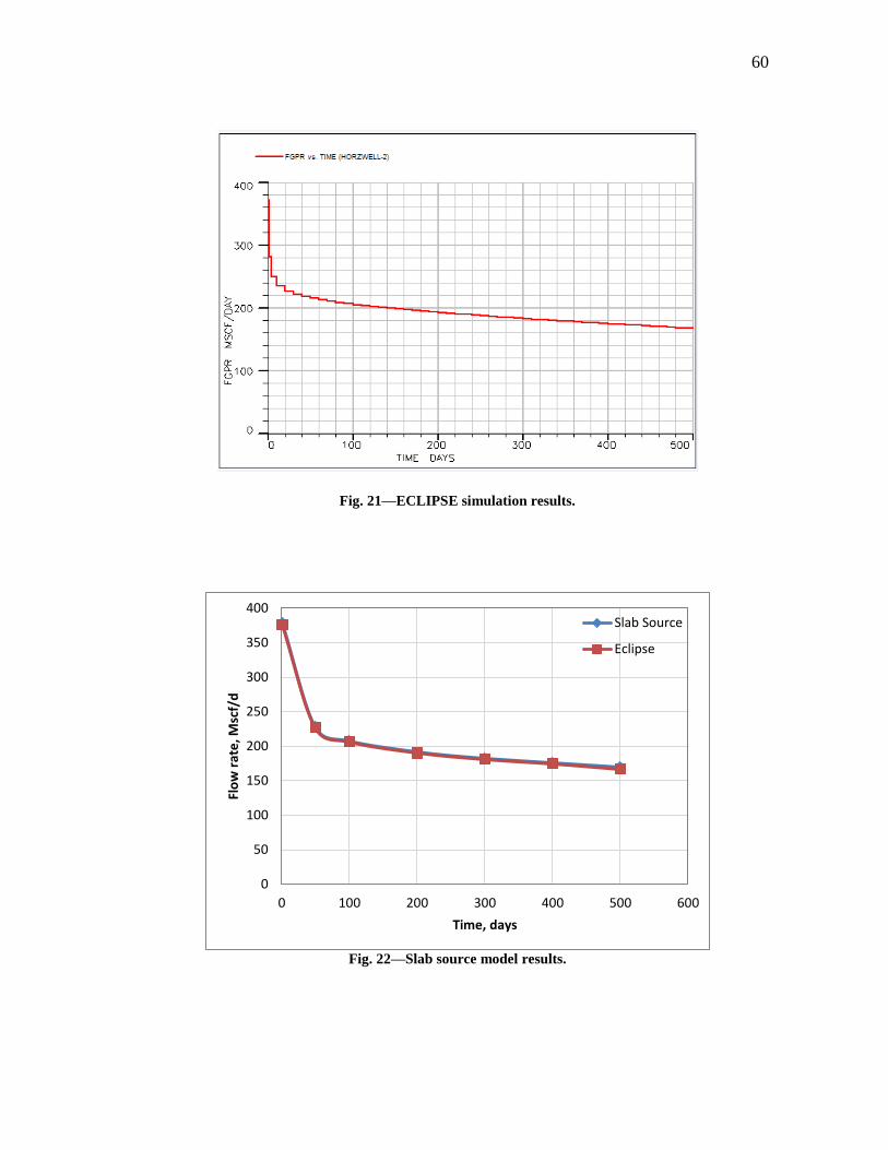
60

Fig. 21—ECLIPSE simulation results.

Fig. 22—Slab source model results.

0

50

100

150

200

250

300

350

400

0 100 200 300 400 500 600

Flo

w r

ate

, Msc

f/d

Time, days

Slab Source

Eclipse

61

CHAPTER IV

RESULTS AND DISCUSSION

In this chapter, the Slab source method is applied to cases of complex well or fractured

horizontal well schematic to show how to optimize the production of such wells by using

the developed method.

Examples of horizontal well with different wellbore length, a horizontal well with

single or multiple transverse fractures intercepts horizontal well are presented first. Then

three field examples are used to show the procedure of the model application with one

example for low permeability unconventional reservoir, and the other moderate

permeability conventional reservoir.

4.1 Synthetic Model

In this section, synthetic examples are used to illustrate how to use the Slab model to

optimize well design for horizontal wells and horizontal wells with fractures. The input

data used in this section is shown in Table 10.

62

Table 10—Input data for synthetic examples.

Reservoir type Tight gas

Formation type Sandstone





Horizontal wellbore length, l 1000, 2000, 3000, 3500 ft

Porosity, 9.0%





Reveal Data

Horizontal permeability, kh 0.1, 0.01, 0.001 md

Vertical permeability, kv 0.01, 0.001, 0.0001 md


4.1.1 Horizontal Well

To product tight gas reservoir, horizontal wells are more efficient compared with vertical

wells. The length of the horizontal laterals relative to the reservoir drainage dimension

will is a key parameter for well production. In general, for tight formation since mobility

dominates the production, the longer the wellbore length, the higher the production rate.

Comparing to the drawdown of the reservoir, the pressure drop along the wellbore is

usually not significant, therefore the pressure drop along the wellbore is neglected in

63

these examples. The well was placed in the middle of the reservoir. Fig. 23 is the

schematic for this study. This resembles an open-hole completion.

Fig. 23—Set up for horizontal well.

Fig. 24 and 25 show the production performance for the horizontal well under

transient flow condition for relatively low permeability (0.01-md, in Fig. 24), and

moderate permeability (0.1-md, Fig. 25). At the same drawdown, with low permeability,

longer wellbore keeps significant advantage through the production period of 500 days

(Fig. 24), but for higher permeability (0.1-md), the benefit of longer wellbore diminishes

and rate declines much faster for longer wellbore compared with short wellbore (Fig.

25). It is necessary to point out that when permeability is higher than 0.1-md, the initial

rate is significant and pressure drop in the wellbore should be considered in this case.

L

h b

a

a

z y

x

64

Fig. 24— Effect of wellbore length on production rate for kh=0.01md, kv=0.005md.

Fig. 25— Effect of wellbore length on production rate for kh=0.1md, kv=0.01md.

0.00

0.20

0.40

0.60

0.80

1.00

1.20

0 100 200 300 400 500 600

Flo

w r

ate

, MM

scf/

day

Time, days

L=1000ft

L=2000ft

L=3000ft

L=4000ft

0

1

2

3

4

5

6

7

0 100 200 300 400 500 600

Flo

w r

ate

, MM

scf/

day

Time, days

L=1000ft

L=2000ft

L=3000ft

L=4000ft

65

The advantage of a longer well length reaches a plateau when the wellbore length is

close to the reservoir dimension. Since longer length will cost more in drilling and

completion, there should be an optimal length which is not only directly related to the

reservoir dimension but also affected by the reservoir properties, such as permeability.

As shown in Fig. 26, the longer the wellbore is, the better the production is. For

relatively low permeability reservoir, the performance will be good when a really long

horizontal wellbore placed in reservoir. Fig. 27 and 28 show that after 3000-ft length,

the production increase reaches a plateau. Beyond this point, increasing wellbore length

will no increase the production rate enough to justify the addiction costs of creating a

longer wellbore. For different reservoir conditions, the optimal length varies, and the

optimal length should be identified for individual cases. This can be clearly

demonstrated that when permeability is relatively low the horizontal well would be

benefit compared to moderate permeability reservoir. In the same reservoir dimension,

the longer the wellbore length in low permeability gives more production increase ration

compared to the one in high permeability.

Realizing that even the flow rate of horizontal wells in low permeability formations

may not be high enough to cause a significant pressure drop in the wellbore, it does not

limit the case that frictional pressure will affect the well performance. When wellbore

length increases it will increase the frictional pressure in the wellbore in two counts:

longer horizontal wells can also limit the well performance, the pressure drop in the

wellbore in such situation should be considered when designing the wellbore length.

66

Fig. 26—Effects of wellbore length on cumulative production (kh=0.01md).

Fig. 27—Effects of wellbore length on cumulative production (kh=0.1md).

0

0.05

0.1

0.15

0.2

0.25

0.3

0.35

0.4

0.45

1 2 3 4

Cu

mu

lati

ve p

rod

uct

ion

, Bsc

f

Wellbore length, ft

0

0.5

1

1.5

2

2.5

1000 2000 3000 4000

Cu

mu

lati

ve p

rod

uct

ion

, Bsc

f

Wellbore length, ft

67

Fig. 28—Percentage increases in cumulative production

due to wellbore length increase.

4.1.2 Multiple Fractures with Infinite Conductivity

Superposition method is applied to study the cases of multiple transverse fractures along

a horizontal well. We compare the production rate for horizontal well with five, ten,

fifteen, and twenty fractures. All the fractures have the same dimensions which are 500-

ft (half length)*0.25-in (width)*50-ft (height), and each fracture is treated as one source.

Fig. 29 to 31 show the results of well performances for three different reservoir

permeabilities. For a high-perm gas reservoir, fracture number is a sensitive parameter to

make hydraulic fracturing attractive. When the number of fractures is too high, benefit of

adding more fractures diminishes. For low-perm gas formations, wells with more

fractures are more likely to perform better than wells with fewer fractures. The more

0.2

0.3

0.4

0.5

0.6

0.7

0.8

1500 2000 2500 3000 3500 4000 4500

Pro

du

ctio

n in

cre

ase

rat

io

Wellbore length, ft

k=0.1md

k=0.01md

68

fractures that can be placed along the wellbore, the higher production rate will be. As

studied before (Zhu et al., 2007; Bagherian et al., 2010), there may be a maximum

number of fractures, and above that number, more fractures will not bring more benefit

to the well production. The optimal fracture spacing also depends on the stress field

change while fracturing each stage (Roussel and Sharma, 2010; Suri and Sharma, 2009),

and completion limitations (how many fractures can actually be placed along a

wellbore). All these should be considered when design a multi-stage fracture treatment

in additional to maximum production rate.

Fig. 29—Cases comparison for kh=0.1md and kv=0.01md.

0

10

20

30

40

50

60

70

0 100 200 300 400 500 600

Flo

w r

ate

, MM

scf/

day

Time, days

5 fracs

10 fracs

15 fracs

20 fracs

69

Fig. 30— Cases comparison for kh=0.01md and kv=0.001md.

Fig. 31— Cases comparison for kh=0.001md and kv=0.0001md.

0

2

4

6

8

10

12

0 100 200 300 400 500 600

Flo

w r

ate

, MM

scf/

day

Time, days

5 fracs

10 fracs

15 fracs

20 fracs

0

0.5

1

1.5

2

2.5

3

3.5

4

4.5

5

0 100 200 300 400 500 600

Flo

w r

ate

, MM

scf/

d

Time, days

5 fracs

10 fracs

15 fracs

20 fracs

70

Noticed that the results show that a horizontal well with 20 fractures produces about

five times more than the production rate of a horizontal well with 5 fractures at early

time of production when reservoir permeability is 0.001md. The reason is that for more

fractures, the sources are more evenly distributed in the reservoir, and traveling distance

for the reservoir fluid to research the sources (one of the fractures) becomes smaller,

implying that flow efficiency is improved with more fractures placed along the wellbore.

For reservoir permeability is 0.1-md, the well with 15 and 20 fractures shows almost the

same production rate in Fig. 29, which means in such a reservoir, more fracture number

will not give us more benefit on production. It suggests that ten fractures should be

enough for this reservoir. When reservoir permeability is drop to 0.01-md (Fig. 30), the

horizontal well with 15 fractures still produces significantly more than 10 fractures. But

when placed 20 fractures, the production rate does not increase much compared with 15

fracture case; which means that the fracture number around 15 is optimal for this

reservoir. For reservoir permeability of 0.001-md (Fig. 31), the horizontal well with 20

fractures still gives us a high production rate. We could draw the conclusion that in

extremely low (0.001-md) permeability reservoir, the more hydraulic fractures, the more

it will benefit to the production.

Fig. 32 shows that after 15 fractures, the production increase (rate at any fracture

number compared with the rate at 5 fractures) approaches a constant for k=0.1-md.

Beyond this point, increasing fracture number will not increase the production rate

enough to justify the addiction costs of creating a longer wellbore. For different reservoir

conditions, the optimal fracture number should be identified for individual cases. We

71

also notice that the production increase for k=0.001-md is four times higher compared to

k=0.1-md condition, which is could also draw the conclusion that hydraulic fractures is

an effective way to develop the reservoir with low permeability.

Fig. 32—Production increase ratio as a function of number of fractures.

4.1.3 Fracture with Finite Conductivity

To study pressure drop inside the fracture, we divided the fracture into several segment.

The fracture pressure profile under finite conductivity inner boundary condition is shown

in Fig. 33. It presents that the pressure decreases from the outside boundary to the center

of the fracture. The production distribution is shown in Fig. 34. In this case, we have

0

0.1

0.2

0.3

0.4

0.5

0.6

0.7

0.8

5 10 15 20 25

Pro

du

ctio

n in

cre

ase

rat

io

Fracture number

k=0.1 md

k=0.01 md

k=0.001 md

72

five fractures along the horizontal well and each fracture has 9 segments. Because of the

pressure drawdown, the production rate is lower than infinite conductivity condition.

Fig. 33—Fracture pressure profile for kh=0.1md, kv=0.01md, and kf=50000md.

1795

1800

1805

1810

1815

1820

1825

1830

1835

0 2 4 6 8 10

Pre

ssu

re,p

sia

Segment number

1

2

3

4

6

7

8

9 5

73

Fig. 34—Infinite conductivity vs. finite conductivity for kh=0.1md, kv=0.01md, and kf=50000md.

Fig. 35 shows the production distribution for each fracture along the horizontal

wellbore for 50 days. The profile shows that the flow rate for the first and the last

fracture at the both ends of horizontal well are the highest followed by fracture 2 and 4,

and the least flow rate is from fracture 3. Since the first and the last fracture have more

drainage area compared to the fractures in the middle, the production rate is the highest

as show in Fig. 36. This additional drainage also contributes to fracture 2 and 4. The

fracture 2 and 4 compared with fracture 3 have higher flow rate.

0

5

10

15

20

25

30

35

0 100 200 300 400 500 600

Flo

w r

are

, MM

scf/

day

Time, days

finite conductivity

infinite conductivity

74

Fig. 35—Flow rate profile for each fracture.

Fig. 36—Flow region for each fracture.

0

1

2

3

4

5

6

7

8

0 1 2 3 4 5 6

Flo

w r

ate

, MM

scf/

day

Fracture number

75

4.1.4 Complex Fracture System

The slab source method could also be used for complex fracture systems. The complex

fracture system is defined as multiple hydraulic fractures placed along a horizontal well

in a natural fracture formation. The hydraulic fractures that connect with the wellbore

are the mean fractures and the natural fractures are branch fractures which only connect

with the main fractures. The fluid inside of the branch fractures directly flows into the

main fractures. For the main fractures, the fluid of the main fracture is from both the

reservoir and the branch fractures and flows to the wellbore. We considered each

hydraulic fracture and natural fracture is a separate source, and the sources will be

affected by the other sources in the system. Superposition method is applied to capture

the internal affection among the sources.

Fig. 37 shows a randomly generate natural fracture network with 20 hydraulic

fractures. The natural fracture length is from 100 to 500-ft and the width is 0.08 to 0.1-

in. For 20 natural fractures, only seven of them are connected with the hydraulic

fractures. One of the natural fractures connects two of the hydraulic fractures. As

mentioned before, we divided the natural fracture into two parts and each of them is

connect with the hydraulic fractures near it. The input data for this case is shown in

Table 11.

76

Fig. 37— Randomly generated complex fracture system.

.

The result is shown below in Fig. 38. The results show that both the hydraulic

fractures and natural fractures would produce. At early time, the hydraulic fractures

produce much more than natural fractures, but after 300 days, the flow rate from

hydraulic fractures is 4.5 times more than natural fractures.

HW

NF1

NF2

NF3

NF4 NF5

NF6

NF7

77

Table 11—Input data for complex fracture system.





Porosity, 0.09 ft








Horizontal well length, L 3000 ft

Hydraulic Fractures




Natural Fracture No. Fracture length, xf Fracture width, wf

1 237 0.007

2 594 0.007

3 260 0.008

4 250 0.009

5 257 0.008

6 528 0.005

7 371 0.008

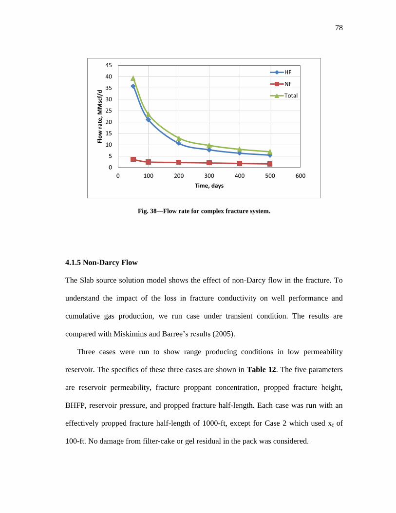
78

Fig. 38—Flow rate for complex fracture system.

4.1.5 Non-Darcy Flow

The Slab source solution model shows the effect of non-Darcy flow in the fracture. To

understand the impact of the loss in fracture conductivity on well performance and

cumulative gas production, we run case under transient condition. The results are

compared with Miskimins and Barree’s results (2005).

Three cases were run to show range producing conditions in low permeability

reservoir. The specifics of these three cases are shown in Table 12. The five parameters

are reservoir permeability, fracture proppant concentration, propped fracture height,

BHFP, reservoir pressure, and propped fracture half-length. Each case was run with an

effectively propped fracture half-length of 1000-ft, except for Case 2 which used xf of

100-ft. No damage from filter-cake or gel residual in the pack was considered.

0

5

10

15

20

25

30

35

40

45

0 100 200 300 400 500 600

Flo

w r

ate

, MM

scf/

d

Time, days

HF

NF

Total

79

Table 12—Cases for non-Darcy flow study.

Case Reservoir

Perm (md)

Proppant Conc. Frac

Height (ft)

BHFP

(psi)

Reservoir Pressure

(pai)

xf

(ft)

1 0.01 1.0 100 1000 4000 1000

2 0.01 1.0 100 1000 4000 100

3 0.1 1.0 100 1000 4000 1000

The results of the three model cases are presented in Fig. 39 thorough 41. The

models show that even for 0.01 md reservoirs the impact of non-Darcy flow can be

significant if the created fracture length is long. In case 1, the slab source result shows a

slightly higher production rate than Barree’s results, but almost the same. The non-Darcy

effects result decrease in cumulative production after 10 years of 11%.

Fig. 39—Cumulative production for case 1.

0

500

1000

1500

2000

2500

3000

3500

0 500 1000 1500 2000 2500 3000 3500 4000

Cu

mu

lati

ve p

rod

uct

ion

, MM

scf

Time, days

Barree Darcy

Barree Non-Darcy

Slab source Darcy

Slab source Non-Darcy

80

Case 2 is similar to case 1 except that the fracture length is decreased from 1000-ft to

100-ft. when the fracture is short, Fig. 40 shows that non-Darcy effects are not

significant.

Fig. 40—Cumulative production for Case 2.

Fig. 41 shows the results for Case 3. This case the reservoir permeability is increase

to 0.1-md. In this case the result shows that the non-Darcy flow effects are magnified.

The difference in production after 10 years is 18%. The difference is caused by the high

production which would introduce higher velocity, resulting in significant Non-Darcy

flow effect.

0

200

400

600

800

1000

1200

1400

1600

1800

2000

0 500 1000 1500 2000 2500 3000 3500 4000

Cu

mu

lati

ve p

rod

uct

ion

, MM

scf

Time, Days

Barree Darcy

Barree Non-Darcy

Slab source Darcy


81

Fig. 41—Cumulative production for Case 3.

A summary of the 10-year cumulative production with and without non-Darcy flow

effects for cases 1-3 is shown in Table 13. For the three cases shown, non-Darcy effects

account for a range of 0.5% to 18% difference in cumulative production over ten years.

Table 13—Cumulative production results.

Case Barree’s model Slab source Model

No. Darcy Flow

(MMscf)

Non-Darcy

(MMscf)

Percentage

Change

Darcy Flow

(MMscf)

Non-Darcy

(MMscf)

Percentage

Change

1 3160 2840 11.3 3250 2870 11.6

2 1835 1825 0.5 1850 1830 2.0

3 15000 12700 18.1 16100 12900 19.8

0

2000

4000

6000

8000

10000

12000

14000

16000

0 500 1000 1500 2000 2500 3000 3500 4000

Cu

mu

lati

ve p

rod

uct

ion

, MM

scf

Time, days

Barree Darcy

Barree Non-Darcy

Slab source Darcy


82

4.2 Field Cases

In this section, field examples are used to illustrate how to use the Slab model. Two field

examples are used to show the procedure of the model application with one example for

low permeability unconventional reservoir, and the other moderate permeability

conventional reservoir.

4.2.1 Case1: Unconventional Reservoir (Mayer, shale)

To validate the multiple fracture calculation, we compared the model result with a

published field production history data. The history match is based on a horizontal well

in Marcellus shale as shown in Fig. 42 (Meyer et al., 2010). The horizontal well was

completed with a seven stage fracture treatment over a lateral length of 2100 ft. Seven

stage fracture treatment was completed over the horizontal wellbore. The production log

showed a total gas flow rate of 3.166 MMscf/d and a water rate of 2541 bpd. Stage two

showed a minimal contribution of about 3% of the total production. Therefore, only six

multiple transverse fractures were used to history match. The reservoir and fracture

properties for Marcellus shale is given in Table 14. The Marcellus shale history matched

parameters are given in Table 15.

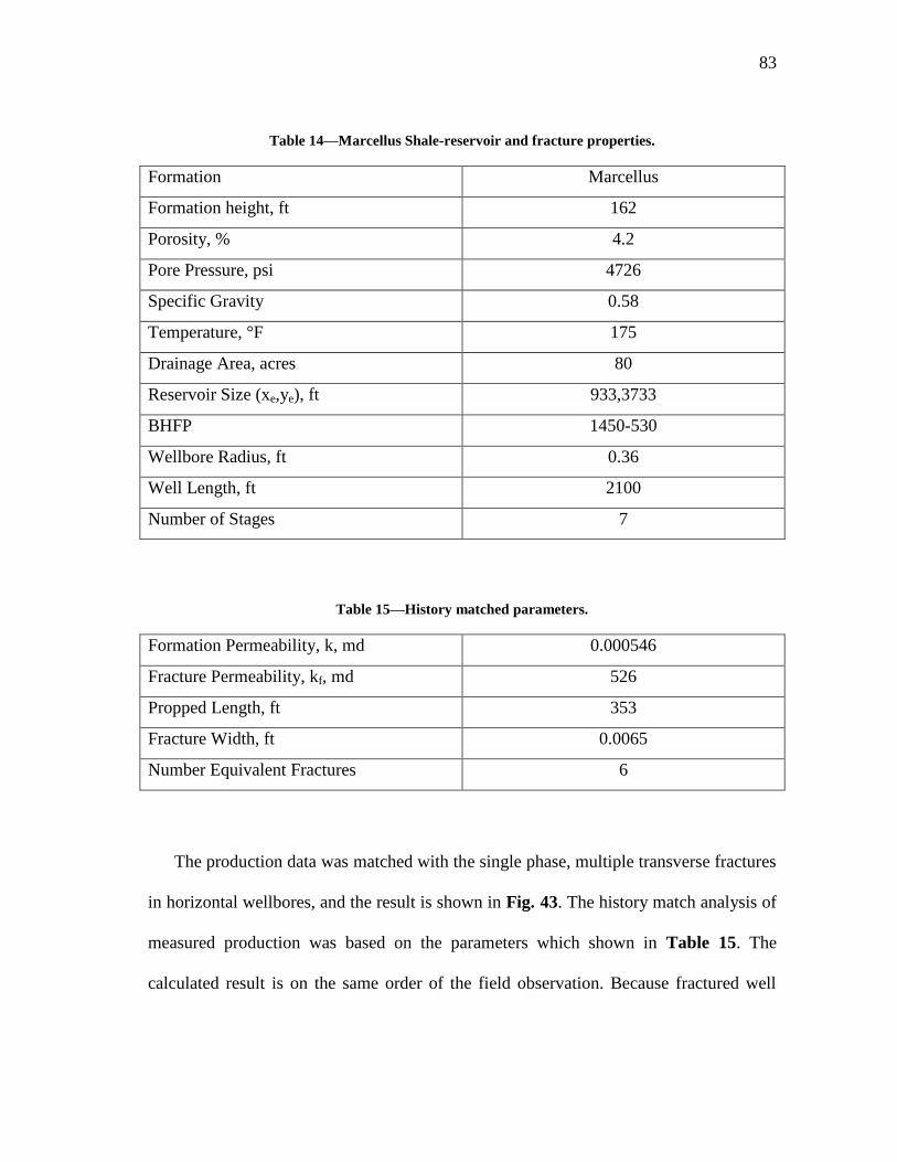
83

Table 14—Marcellus Shale-reservoir and fracture properties.

Formation Marcellus

Formation height, ft 162

Porosity, % 4.2

Pore Pressure, psi 4726

Specific Gravity 0.58

Temperature, °F 175

Drainage Area, acres 80

Reservoir Size (xe,ye), ft 933,3733

BHFP 1450-530

Wellbore Radius, ft 0.36

Well Length, ft 2100

Number of Stages 7

Table 15—History matched parameters.

Formation Permeability, k, md 0.000546

Fracture Permeability, kf, md 526

Propped Length, ft 353

Fracture Width, ft 0.0065

Number Equivalent Fractures 6

The production data was matched with the single phase, multiple transverse fractures

in horizontal wellbores, and the result is shown in Fig. 43. The history match analysis of

measured production was based on the parameters which shown in Table 15. The

calculated result is on the same order of the field observation. Because fractured well

84

performance depends on numerous parameters including reservoir properties and

fracture geometries which both contain uncertainty and it is not surprised that a perfect

match was not obtained. From the results (Fig. 43), the higher production rate at early

time from the slab model could be caused by the assumptions of ideal condition of

fractures and neglected Non-Darcy effect inside fracture. The proppant permeability

used in the history match is the effective permeability. The effective permeability

contains two parts, one is the proppant permeability and the other is the natural fracture

permeability. In this case, the connection between natural fractures and hydraulic

fractures are unknown factor, the source function cannot directly applied in the natural

fracture system. The natural fracture permeability has been represented here as an

effective proppant permeability in the hydraulic fractures.

An average permeability of 377 nanodarcy over a formation thickness of 162 ft that

included the upper and lower Marcellus has been showed by a petrophysical analysis.

The resulting reservoir capacity (kh) was calculated to be 0.061md-ft, an average

reservoir permeability of 555 nanodarcy, and a reservoir capacity of 0.09 md-ft. the

history match results for this case match very well with the information.

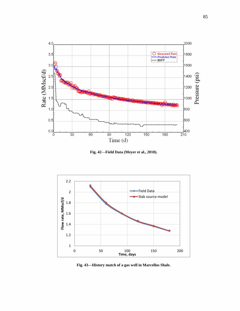
85

Fig. 42—Field Data (Meyer et al., 2010).

Fig. 43—History match of a gas well in Marcellus Shale.

1

1.2

1.4

1.6

1.8

2

2.2

0 50 100 150 200

Flo

w r

ate

, MM

scf/

d

Time, days

Field Data

Slab source model

86

4.2.3 Case2: Moderate Permeability

A gas reservoir is used in the example. The reservoir has multiple layers with significant

contraction in permeability in each layer. The permeability profile is shown in Table 16

and Fig. 44. Layer 3 has the lowest permeability, serving as a vertical isolation in the

formation. In such a reservoir, horizontal well may lose its attraction compared with

vertical well because of low vertical communication. The example compares the well

structure plans including vertical well, vertical well with fracture, slanted well,

horizontal well without fracturing, and horizontal well with multiple transverse fractures.

The input data is shown in Table 17.

Table 16—Permeability summary for layers.

Layer No. Layer Thickness (ft) kh (md) kv (md) Average perm, kh (md)

1 12 0.05-0.5 0.14 0.26

2 6 10.64 5.53 10.64

3 5 0.003 0.003 0.003

4 26 0.2-0.6 0.16 0.36

5 2 2.32 2.32 2.32

6 116 0.1-0.8 0.12 0.25

7 10 1.92 1.92 1.92

8 5 7.55 4.07 7.55

9 18 0.5-2.3 0.89 1.67

87

Table 17—Input data for case study.

Reservoir type Tight gas

Formation type Sandstone





Horizontal wellbore length, l 3000 ft

Porosity, 9.0%





Water specific gravity, w 1.005

Fig. 44—Schematic of the formation.

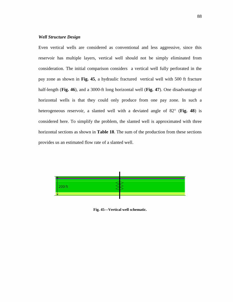
88

Well Structure Design

Even vertical wells are considered as conventional and less aggressive, since this

reservoir has multiple layers, vertical well should not be simply eliminated from

consideration. The initial comparison considers a vertical well fully perforated in the

pay zone as shown in Fig. 45, a hydraulic fractured vertical well with 500 ft fracture

half-length (Fig. 46), and a 3000-ft long horizontal well (Fig. 47). One disadvantage of

horizontal wells is that they could only produce from one pay zone. In such a

heterogeneous reservoir, a slanted well with a deviated angle of 82° (Fig. 48) is

considered here. To simplify the problem, the slanted well is approximated with three

horizontal sections as shown in Table 18. The sum of the production from these sections

provides us an estimated flow rate of a slanted well.

Fig. 45—Vertical well schematic.

89

Fig. 46—Fractured vertical well schematic.

Fig. 47—Horizontal well schematic.

Table 18—Parameter list for slanted well.

Zone No. Layer No. kh, md kv,md

1 1-4 0.72 0.34

2 5-6 0.26 0.2

3 7-9 1.67 0.92

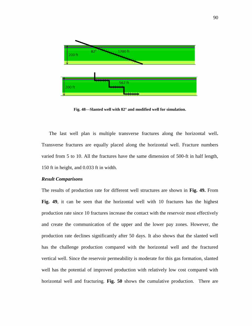
90

Fig. 48—Slanted well with 82° and modified well for simulation.

The last well plan is multiple transverse fractures along the horizontal well.

Transverse fractures are equally placed along the horizontal well. Fracture numbers

varied from 5 to 10. All the fractures have the same dimension of 500-ft in half length,

150 ft in height, and 0.033 ft in width.

Result Comparisons

The results of production rate for different well structures are shown in Fig. 49. From

Fig. 49, it can be seen that the horizontal well with 10 fractures has the highest

production rate since 10 fractures increase the contact with the reservoir most effectively

and create the communication of the upper and the lower pay zones. However, the

production rate declines significantly after 50 days. It also shows that the slanted well

has the challenge production compared with the horizontal well and the fractured

vertical well. Since the reservoir permeability is moderate for this gas formation, slanted

well has the potential of improved production with relatively low cost compared with

horizontal well and fracturing. Fig. 50 shows the cumulative production. There are

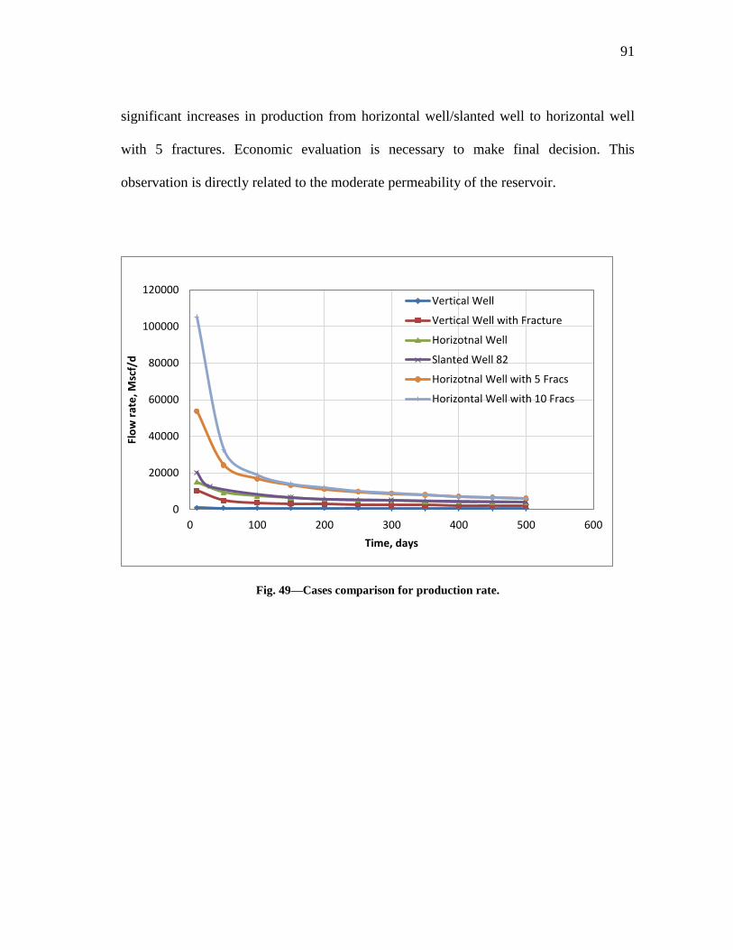
91

significant increases in production from horizontal well/slanted well to horizontal well

with 5 fractures. Economic evaluation is necessary to make final decision. This

observation is directly related to the moderate permeability of the reservoir.

Fig. 49—Cases comparison for production rate.

0

20000

40000

60000

80000

100000

120000

0 100 200 300 400 500 600

Flo

w r

ate

, Msc

f/d

Time, days

Vertical Well

Vertical Well with Fracture

Horizotnal Well

Slanted Well 82

Horizotnal Well with 5 Fracs

Horizontal Well with 10 Fracs

92

Fig. 50—Cases comparison for cumulative production.

0

1000

2000

3000

4000

5000

6000

7000

8000

0 100 200 300 400 500 600

Cu

mu

lati

ve p

rod

uct

ion

, MM

scf

Time, days

Vertical WellVertical Well with FractureHorizotnal WellSlanted Well 82Horizotnal Well with 5 FracsHorizontal Well with 10 Fracs

93

CHAPTER V

CONCLUSIONS

Hydraulic fractures have been used widely today especially in the tight gas reservoir.

Predicting well performance becomes much more difficult compared with conventional

wells. In order to evaluate well performance, we developed a new model. This

dissertation presents well performance models of horizontal wells with/without fractures,

and complex fractures system. The model can be used to generate inflow performance

relationships, study parameter sensitivity, and optimize well designs.

We developed the slab source method as a solution to calculation the well

performance and pressure distribution in a closed, rectangular reservoir under different

boundary conditions. The model can be used for both transient and pseudosteady-state

flow. we have successfully developed and validated a series of solutions for pressure and

production behavior of simple and complex well/fracture configurations such as

horizontal well, multiple fractures, and natural fractures. We also demonstrated the

applicability of the new solution method in predicting production behavior for a

horizontal well with multiple transverse fractures and complex fractures system. The

new method is applied as an optimization and screening tool to obtain the best

completion schematic for development of well design.

The conclusions can be summarized as following:

1. Slab source model was developed successfully to calculate flow problems in

complex reservoir system

94

2. Model can handle horizontal wells with multiple stage fractures in a natural

fracture reservoir.

3. The optimal number of fracture stages is strongly depends on reservoir

permeability. For moderate permeability formation, higher number of fractures

stages does not necessarily yield justified benefit in production. For lower

permeability formation, the higher the fracture number, the better the production.

The optimal number of fractures should be determined by other constrains than

production rate.

4. Non-Darcy flow effects have an influence on flow rates, these decrease can range

from 2% to 20% under a given set of conditions.

5. Long-term production is significantly affected by Non-Darcy conductivity losses,

even in relatively low permeability reservoirs where long fractures are needed.

6. For complex fracture system, the production from natural fractures depends on

natural fracture location, dimension, and connection point with the hydraulic

fractures.

Recommendations

Based on the results of this study, it is recommend that

1. Non-Darcy effects can be added for complex fractures system to count for the

additional pressure and production decrease.

2. A comprehensive two-phase well flow model can be developed in the future.

3. The limitation of the model is that the natural fracture must be parallel to

reservoir boundary.

4. Constant pressure boundary will be appreciated for application.

95

NOMENCLATURE

As = cross-section area of source term, ft2

a = reservoir width, ft

B = formation volume factor

b = reservoir length, ft

ct = compressibility, psi-1

h = reservoir height, ft

kx = permeability in x-direction, md

ky = permeability in y-direction, md

kz = permeability in z-direction, md

l = wellbore length, ft

L =dimensionless reservoir position

pD =dimensionless pressure

pint = initial reservoir pressure, psi

p = average reservoir pressure, psi

pwf = bottomhole pressure, psi

Δp = pressure drawdown, psi

q = flow rate, Mscf/day

T = temperature, °R

tD =dimensionless time

xD = dimensionless reservoir length

96

xf = fracture width, ftyD

yf =dimensionless reservoir width

zD =dimensionless reservoir height

g specific gas gravity, dimensionless

= density, lb/ft3

= porosity, fraction

= viscosity, cp

= time

atm-sec2/gm

ug = cp or g/100-cm-sec

97

REFERENCES

Babu, D.K. and Odeh, A.S. 1988. Productivity of a Horizontal Well Appendices A and

B. Paper SPE 18334 presented at the SPE Annual Technical Conference and

Exhibition, Houston, Texas. 2-5 October.

Bagherian, B., Sarmadivaleh, M., Ghalambor, A., Nabipour, A., Rasouli, V. et al. 2010.

Optimization of Multiple-Fractured Horizontal Tight Gas Well. Paper SPE

127899 presented at the SPE International Symposium and Exhibiton on

Formation Damage Control, Lafayette, Louisiana, USA. 10-12 February.

Cinco-Ley, H. and Samaniego-V., F. 1981. Transient Pressure Analysis for Fractured

Wells. J. Pet Tech. 33 (9): 1748-1766. SPE-7490-PA. DOI: 10.2118/

Cooke Jr., C.E. 1973. Conductivity of Fracture Proppants in Multiple Layers. J. Pet

Tech. 25(09): 1101-1107. SPE-4117-PA. DOI: 10.2118/4117-pa

Carslaw, H. S. and Jaeger, J. C. 1959. Conduction of Heat in Solids, Oxford, UK:

Clarendon Press.

Cramer, D.D. 2004. Analyzing Well Performance in Hydraulically Fractured Gas Wells:

Non-Ideal Cases. Paper SPE 90777 presented at the SPE Annual Technical

Conference and Exhibition, Houston, Texas.26-29 September.

Darcy, H.P.G. 1856. The Public Fountains of the City of Dijon (appendix). Bookseller of

the Imperial Corps of Bridges, Highways and Mines, Quay of Augustins.

Ecrin-Kappa, User Manuel, Version 4.12, Sophia Antipolis, France.

98

Etherington, J.R. 2005. Getting Full Value from Reserves Audits. Paper SPE 95341

presented at the SPE Annual Technical Conference and Exhibition, Dallas,

Texas. 9-12 October .

Forchheimer, P. 1901. Wasserbewegung durch Boden, Vol. 45. Zeits. V. Deutsch, Ing.

Geertsma, J. 1974. Estimating the Coefficient of Inertial Resistance in Fluid Flow

through Porous Media. SPE J. 14 (5): 445-450. SPE-4706-PA DOI:

10.2118/4706-pa

Goode, P.A. and Kuchuk, F.J. 1991. Inflow Performance of Horizontal Wells. SPE Res

Eng 6 (3): 319-323 SPE-21460-PA DOI: 10.2118/21460-pa

Gringarten, A.C. and Ramey Jr., H.J. 1973. The Use of Source and Green's Functions in

Solving Unsteady-Flow Problems in Reservoirs. SPE J. 13 (5): 285-296. SPE-

3818-PA. DOI: 10.2118/3818-pa.

Gringarten, A.C. and Ramey Jr., H.J., and Raghavan, R. 1974. Unsteady-State Pressure

Distribution Created by a Well With a Single Infinite-Conductivity Vertical

Fracture. SPE J. 14 (4): 347-360. SPE-4051-PA. DOI: 10.2118/4051-pa.

Meyer, B.R., Bazan, L.W., Jacot, R.H., and Lattibeaudiere, M.G. 2010. Optimization of

Multiple Transverse Hydraulic Fractures in Horizontal Wellbores. Paper SPE

131732 presented at the SPE Unconventional Gas Conference, Pittsburgh,

Pennsylvania, USA. 23-25 February.

Miskimins, J.L., Lopez, H.D.J., and Barree, R.D. 2005. Non-Darcy Flow in Hydraulic

Fractures: Does It Really Matter? Paper SPE 96389 presented at the SPE Annual

Technical Conference and Exhibition, Dallas, Texas. 9-12 October.

99

Ouyang, L.-B., Thomas, L.K., Evans, C.E., and Aziz, K. 1997. Simple but Accurate

Equations for Wellbore Pressure Drawdown Calculation. Paper SPE 38314

presented at the SPE Western Regional Meeting, Long Beach, California. 25-27

June.

Ozkan, E., Sarica, C., Haciislamoglu, M., and Raghavan, R. 1995. Effect of

Conductivity on Horizontal Well Pressure Behavior. SPE Advanced Technology

Series 3 (1): 85-94. SPE-24683-PA. DOI: 10.2118/24683-pa

Penny, G.S. and Jin, L. 1995. The Development of Laboratory Correlations Showing the

Impact of Multiphase Flow, Fluid, and Proppant Selection Upon Gas Well

Productivity. Paper SPE 30494 presented at the SPE Annual Technical

Conference and Exhibition, Dallas, Texas. 22-25 October.

Roussel, N. P., and Sharma, M. M., 2010. Optimizing Fracture Spacing and Sequencing

in Horizontal Well Fracturing. Paper SPE 127986 presented at SPE International

Symposium and Exhibition on Formation Damage Control , Lafayette,

Louisiana, USA. 10-12 February.

Smith, M.B., Bale, A., Britt, L.K., Cunningham, L.E., Jones, J.R. et al. 2004. An

Investigation of Non-Darcy Flow Effects on Hydraulic Fractured Oil and Gas

Well Performance. Paper SPE 90864 presented at the SPE Annual Technical

Conference and Exhibition, Houston, Texas. 26-29 September.

Suri. A., and Sharma, M.M., 2009. Fracture Grouwth in Horiozntal injectors. Paper SPE

119379 presented at SPE Hydraulic Fracturing Technology Conference,

Woodlands, Texas, USA. 19-21 January.

100

Valko, P.P. and Amini, S. 2007. The Method of Distributed Volumetric Sources for

Calculating the Transient and Pseudosteady-State Productivity of Complex Well-

Fracture Configurations. Paper SPE 106279 presented at the SPE Hydraulic

Fracturing Technology Conference, College Station, Texas USA. 29-31 January.

Zhu, D., Magalhaes, F.V., and Valko, P. 2007. Predicting the Productivity of Multiple-

Fractured Horizontal Gas Wells. Paper SPE 106280 presented at the SPE

Hydraulic Fracturing Technology Conference, College Station, Texas USA. 29-

31 January.

101

APPENDIX A

The use of Green’s functions in the theory of potential is well known. The function is

most conveniently defined for the closed surface S as the potential which vanishes over

the surface, and is infinite as 1/r, when r is zero, at the point p(x’,y’,z’) inside the

surface. If this solution of the equation 02 u is denoted by G(p). The solution with

no infinity inside S and an arbitrary value V over the surface is given by

VdSpGn

)(4

1

A1

n

denoting differentiation along the outward drawn normal.

We proceed to show how a similar function may be employed with advantage in the

mathematical theory of the conduction of heat. In this case we shall take the Green’s

function as the temperature at (x,y,z) at the time t, due to an instantaneous point source

of strength unity generated at the point p(x’,y’,z’) at time τ, the solid being initially at

zero temperature, and the surface being kept at zero temperature. This solution is written

),'',',,,( tzyxzyxF (τ>t) A2

and u satisfies the equation

ukt

2

(τ>t) A3

However, since t only enters in the form (t-τ), we have also

02

uk

t

(τ<t) A4

102

Further,

t

u 0)lim(at all points inside S, expect at point (x’,y’,z’), where the solution

takes the from

tk

zzyyxx

tk 4

'''exp

8

1222

2/3 A5

Finally, at the surface S, u=0 (τ<t).

Let v be the temperature at the time t in this solid due to the surface temperature

ϕ(x,y,z,t) and the initial temperature f(x,y,z)

Then v satisfies the equations

vkt

v 2

(t>0) A6

v=f(x,y,z) inially, inside S

v=ϕ(x,y,z) at S, when t>0

Also, since the time τ of our former equations lies within the interval for t, we have

vkt

v 2

τ<t A7

v=ϕ(x,y,z) at the surface.

Therefore,

uvvuku

vv

ut

uv 22)(

A8

and

dxdydzduvvukddxdydzuv

tt

0

22

0

)( A9

103

The triple integrate being taken into the solid, and ε being any positive number less than

t.

Interchanging the order of integration on the left-side of this equation and applying

Green’s theorem to the right-hand side. We have

dxdydzuvkdxdydzuv t 0

t

ddSn

uv

n

vuk

0

t

i

ddSn

uvk

0

A10

where in

denotes differentiation along the inward-drawn normal, and we have used the

condition that u vanishes at the surface.

Now take the limit as ε tends to zero. The left-side gives

dxdydzvudxdydzuV tP 00 A11

The first integral being taken though an element of volume including the point

p(x’,y’,z’), where the function u becomes infinite at t=τ. The second integral being taken

through the solid, and the PV stands for the value of v at the point p(x’,y’,z’) at the

time t. but since u is the temperature at the time t due to a unit source at (x’,y’,z’) at time

τ, 1 dxdydzu t and we have

t

i

P ddSn

uvktdxdydzvuV

0

00

104

t

i

ddSn

uzyxktdxdydzzyxfu

0

0 ),,,(),,( A12

as the temperature at (x’,y’,z’) at the time t due to the initial distribution f(x,y,z) and the

surface temperature ϕ(x,y,z,t).

In the case of radiation at the surface, the Green’s function u is taken as the

temperature at (x,y,z) at time t due to an instantaneous point source of strength unity

generated at (x’,y’,z’) at time τ, radiation taking place at the surface into a medium at

zero temperature.

Linear flow in the semi-infinite solid x>0

Fig. 51—Semi-infinite solid reservoir and slab source.

The solution is

')(4

)'(exp

)(4

1 2

2

2

dxtk

xx

tk

f

w

f

w

xx

xx

A13

xf

x 0

105

For linear flow in reservoir, 0<x<a, the slab source is at x=xw as shown in . Initial

temperature f(x), bounding planes kept at zero.

Starting with the source f(xw)dxw at xw, we have to take the images of this source in

the planes x=0 and x=a, a source and a sink alternating so that the boundaries may be

kept at zero. In this way we have sources at the points xw+2na and sinks at the points –

xw+2na, where n is zero or any positive or negative integer.

Fig. 52—Finite solid bounded by the planes x=0 and x=a, slab source.

Thus, we have finally

')(4

)'2(exp

)(4

1 2

2

2

n

xx

xx

dxtk

xnax

tkv

f

w

f

w

')(4

)'2(exp

2

2

2

n

xx

xx

dxtk

xnax

f

w

f

w

A14

Because of the Poisson’s summation formula,

a 0

x xf

xw

106

1

22

22

)'(cos21

)(

)(4

)'2(exp

n

a

tkn

n

ea

xxn

a

tk

tk

xnax

1

22

22

)'(cos21

)(

)(4

)'2(exp

n

a

tkn

n

ea

xxn

a

tk

tk

xnax

A15

Therefore, A14 could be written as

a

xn

a

xn

a

xn

a

tkn

nx

a

a

xv wf

nf

f

coscos

2sinexp

141

12

22

A16

107

VITA

Jiajing Lin received her Bachelor of Science degree in electronic engineering

from Beijing Institute of Technology in 2004. She attended the petroleum engineering

program at the University of Louisiana at Lafayette in September 2004 and received her

Master of Science degree in August 2006. After that, she entered in the engineering

school at Texas A&M University and completed her Ph.D. in petroleum engineering in

2011.

She may be reached at:

Department of Petroleum Engineering

Room 712, RICH Building

College Station, TX 77843-3116

Her Email is [email protected]

THE PERFORMANCE OF FRACTURED HORIZONTAL WELL...

Documents

Transcript of THE PERFORMANCE OF FRACTURED HORIZONTAL WELL...