The Pdf Of Irradiance For A Free-space Optical ...

University of Central Florida University of Central Florida

STARS STARS

Electronic Theses and Dissertations, 2004-2019

2010

The Pdf Of Irradiance For A Free-space Optical Communications The Pdf Of Irradiance For A Free-space Optical Communications

Channel: A Physics Based Model Channel: A Physics Based Model

David Wayne University of Central Florida

Part of the Electrical and Electronics Commons

Find similar works at: https://stars.library.ucf.edu/etd

University of Central Florida Libraries http://library.ucf.edu

This Doctoral Dissertation (Open Access) is brought to you for free and open access by STARS. It has been accepted

for inclusion in Electronic Theses and Dissertations, 2004-2019 by an authorized administrator of STARS. For more

information, please contact [email protected].

STARS Citation STARS Citation Wayne, David, "The Pdf Of Irradiance For A Free-space Optical Communications Channel: A Physics Based Model" (2010). Electronic Theses and Dissertations, 2004-2019. 4300. https://stars.library.ucf.edu/etd/4300

https://stars.library.ucf.edu/



https://stars.library.ucf.edu/etd

http://network.bepress.com/hgg/discipline/270?utm_source=stars.library.ucf.edu%2Fetd%2F4300&utm_medium=PDF&utm_campaign=PDFCoverPages

https://stars.library.ucf.edu/etd

http://library.ucf.edu/

mailto:[email protected]

https://stars.library.ucf.edu/etd/4300?utm_source=stars.library.ucf.edu%2Fetd%2F4300&utm_medium=PDF&utm_campaign=PDFCoverPages



THE PDF OF IRRADIANCE FOR A FREE-SPACE OPTICAL COMMUNICATIONS CHANNEL: A PHYSICS BASED MODEL

by

DAVID T. WAYNE B.S.E.E. Grand Valley State University, 2004

M.S.E.E. University Central Florida, 2006 M.S. University Central Florida, 2009

A dissertation submitted in partial fulfillment of the requirements for the degree of Doctor of Philosophy

in the School of Electrical Engineering and Computer Science in the College of Engineering and Computer Science

at the University of Central Florida Orlando, FL

Summer Term 2010

Major Professor: Ronald L. Phillips

ii

ABSTRACT

An accurate PDF of irradiance for a FSO channel is important when designing a laser radar,

active laser imaging, or a communications system to operate over the channel. Parameters such

as detector threshold level, probability of detection, mean fade time, number of fades, BER, and

SNR are derived from the PDF and determine the design constraints of the receiver, transmitter,

and corresponding electronics. Current PDF models of irradiance, such as the Gamma-Gamma,

do not fully capture the effect of aperture averaging; a reduction in scintillation as the diameter

of the collecting optic is increased. The Gamma-Gamma PDF of irradiance is an attractive

solution because the parameters of the distribution are derived strictly from atmospheric

turbulence parameters; propagation path length, Cn2, l0, and L0. This dissertation describes a

heuristic physics-based modeling technique to develop a new PDF of irradiance based upon the

optical field. The goal of the new PDF is three-fold: capture the physics of the turbulent

atmosphere, better describe aperture averaging effects, and relate parameters of the new model to

measurable atmospheric parameters.

The modeling decomposes the propagating electromagnetic field into a sum of independent

random-amplitude spatial plane waves using an approximation to the Karhunen-Loeve

expansion. The scattering effects of the turbulence along the propagation path define the

random-amplitude of each component of the expansion. The resulting PDF of irradiance is a

double finite sum containing a 0K Bessel function. The newly developed PDF is a

generalization of the Gamma-Gamma PDF, and reduces to such in the limit.

iii

An experiment was setup and performed to measure the PDF of irradiance for several receiver

aperture sizes under moderate to strong turbulence conditions. The propagation path was

instrumented with scintillometers and anemometers to characterize the turbulence conditions.

The newly developed PDF model and the GG model were compared to histograms of the

experimental data. The new PDF model was typically able to match the data as well or better

than the GG model under conditions of moderate aperture averaging. The GG model fit the data

better than the new PDF under conditions of significant aperture averaging. Due to a limiting

scintillation index value of 3, the new PDF was not compared to the GG for point apertures

under strong turbulence; a regime where the GG is known to fit data well.

iv

ACKNOWLEDGMENTS

I would like to thank Dr. Ronald Phillips and Dr. Larry Andrews for their time, commitment, and

dedication to my education. I would like to thank Dr. John Stryjewski for his time, conversation,

and direction regarding the practical aspects of experimentation and project management. I

would like to thank Mr. Brad Griffis for his help, instruction, and guidance with the experimental

setup. I would like to thank the researchers at Harris Corporation: Dr. Geoff Burdge and Mr.

Michael Borbath for their support and use of equipment and Mr. Robert Peach for his assistance

in the early phases of data collection. Finally, I am indebted to Jamie for her endless patience,

encouragement, and support.

v

TABLE OF CONTENTS

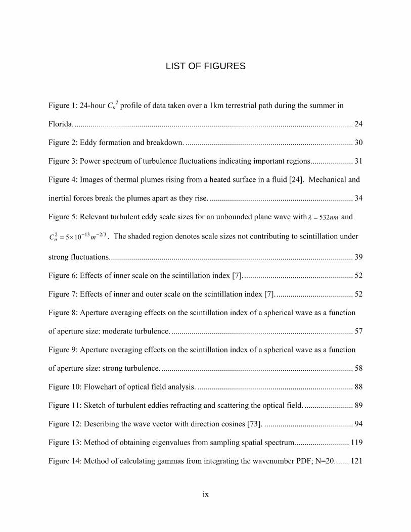
LIST OF FIGURES ....................................................................................................................... ix

LIST OF TABLES ....................................................................................................................... xiii

LIST OF SYMBOLS ................................................................................................................... xiv

1 INTRODUCTION .................................................................................................................. 1

2 BACKGROUND .................................................................................................................... 5

2.1 Random Processes .......................................................................................................... 5

2.1.1 Stationarity, homogeneity, isotropy, and ergodicity ............................................... 5

2.1.1.1 Testing for stationarity ........................................................................................ 7

2.1.2 Probability density function .................................................................................... 9

2.1.2.1 Histogram .......................................................................................................... 13

2.1.3 Structure function.................................................................................................. 16

2.1.4 Averaging time ...................................................................................................... 18

3 ATMOSPHERIC TURBULENCE ....................................................................................... 19

3.1 Solution Techniques for the Stochastic Helmholtz Equation ....................................... 19

3.2 Refractive Index Structure Parameter, Cn2 .................................................................... 21

3.3 Power Spectrum Models ............................................................................................... 24

3.4 Turbulence Generation .................................................................................................. 28

3.4.1 Birth of an eddy .................................................................................................... 32

3.5 Thermal Plumes and Near Ground Effects (Near-Ground Cn2 Fluctuations) ............... 33

3.6 Taylor’s Frozen Turbulence Hypothesis ....................................................................... 35

3.7 Scale Sizes of Optical Turbulence ................................................................................ 37

vi

3.8 Stochastic Field Properties ............................................................................................ 39

3.8.1 Second-order statistics .......................................................................................... 40

3.8.2 Fourth-order statistics ........................................................................................... 42

3.8.3 Coherence function of a stochastic field ............................................................... 44

3.8.4 Karhunen-Loeve expansion .................................................................................. 45

3.9 Effects of Turbulence on Optical Waves ...................................................................... 49

3.9.1 Scintillation ........................................................................................................... 49

3.9.2 Aperture averaging ................................................................................................ 56

4 PREVIOUS & CURRENT PDF MODELS ......................................................................... 60

4.1 Nakagami m-Distribution ............................................................................................. 61

4.2 Lognormal Distribution ................................................................................................ 64

4.3 K Distribution ............................................................................................................... 66

4.4 Universal Distribution ................................................................................................... 69

4.5 I-K Distribution ............................................................................................................. 71

4.6 Generalized K-Distribution ........................................................................................... 74

4.7 Lognormally Modulated Exponential ........................................................................... 76

4.8 Lognormally Modulated Rician .................................................................................... 78

4.9 Gamma-Gamma Distribution ........................................................................................ 80

5 PHYSICAL MODELING ..................................................................................................... 86

5.1 Overview of Model Development ................................................................................ 87

5.2 Decomposing the Complex Envelope of a Stochastic Field ......................................... 89

5.3 Angular Spectrum ......................................................................................................... 92

5.4 2-D Fourier Transform of the Mutual Coherence Function .......................................... 95

vii

5.4.1 Relating angular spectrum and spatial spectrum .................................................. 98

5.5 Wavenumber PDF ....................................................................................................... 100

5.6 Probability Density Function of Received Irradiance ................................................. 102

5.7 Statistical Moments of Irradiance and Scintillation Index .......................................... 109

5.7.1 First moment of irradiance .................................................................................. 109

5.7.2 Second moment of irradiance ............................................................................. 112

5.7.3 Scintillation index ............................................................................................... 114

5.8 Relating Model Parameters to Physical Quantities ..................................................... 116

5.8.1 Sampling the spatial spectrum ............................................................................ 117

5.8.2 Sampling the wavenumber PDF ......................................................................... 120

6 EXPERIMENTATION ....................................................................................................... 122

6.1 Overview ..................................................................................................................... 122

6.2 Equipment ................................................................................................................... 125

6.2.1 Scintillometer – path averaged Cn2 ..................................................................... 125

6.2.2 Scintillometer – path averaged Cn2 and l0 ........................................................... 130

6.2.3 Transmitter system .............................................................................................. 132

6.2.4 Receiver system .................................................................................................. 133

6.3 Data ............................................................................................................................. 135

7 DISCUSSION ..................................................................................................................... 152

8 CONCLUSION ................................................................................................................... 159

APPENDIX A SCINTILLATON INDEX OF A SPHERICAL WAVE INCLUDING

APERTURE AVERAGING ....................................................................................................... 163

APPENDIX B HANKEL TRANSFORM OF MCF: b = 5/3 .................................................... 166

viii

APPENDIX C CHARACTERISTIC FUNCTION .................................................................... 172

APPENDIX D INTERPRETING POWER METER OUTPUT ................................................ 178

APPENDIX E NUMERICAL INACCURACIES OF NEW PDF AT LOW IRRADIANCE .. 182

LIST OF REFERENCES ............................................................................................................ 187

ix

LIST OF FIGURES

Figure 1: 24-hour Cn2 profile of data taken over a 1km terrestrial path during the summer in

Florida. .......................................................................................................................................... 24

Figure 2: Eddy formation and breakdown. ................................................................................... 30

Figure 3: Power spectrum of turbulence fluctuations indicating important regions. .................... 31

Figure 4: Images of thermal plumes rising from a heated surface in a fluid [24]. Mechanical and

inertial forces break the plumes apart as they rise. ....................................................................... 34

Figure 5: Relevant turbulent eddy scale sizes for an unbounded plane wave with nm532=λ and

32132 105 −−×= mCn . The shaded region denotes scale sizes not contributing to scintillation under

strong fluctuations. ........................................................................................................................ 39

Figure 6: Effects of inner scale on the scintillation index [7]. ...................................................... 52

Figure 7: Effects of inner and outer scale on the scintillation index [7]. ...................................... 52

Figure 8: Aperture averaging effects on the scintillation index of a spherical wave as a function

of aperture size: moderate turbulence. .......................................................................................... 57

Figure 9: Aperture averaging effects on the scintillation index of a spherical wave as a function

of aperture size: strong turbulence. ............................................................................................... 58

Figure 10: Flowchart of optical field analysis. ............................................................................. 88

Figure 11: Sketch of turbulent eddies refracting and scattering the optical field. ........................ 89

Figure 12: Describing the wave vector with direction cosines [73]. ............................................ 94

Figure 13: Method of obtaining eigenvalues from sampling spatial spectrum. .......................... 119

Figure 14: Method of calculating gammas from integrating the wavenumber PDF; N=20. ...... 121

x

Figure 15: Layout of equipment on 1km laser range. Three scintillometers were used to provide

path-averaged Cn2 and l0. Three 3-axis anemometers provided the crosswind at points along the

path. ............................................................................................................................................. 124

Figure 16: Optical layout of transmitter system. ........................................................................ 133

Figure 17: Optical layout of receiver system. ............................................................................. 134

Figure 18: Receiving telescope with aperture in place. .............................................................. 135

Figure 19: New PDF, GG PDF, and histogram of data; 1.5mm aperture, Cn2 = 5.00 x10-14, ρsp=

7.16mm. ...................................................................................................................................... 139


5.21mm. ...................................................................................................................................... 140


5.03mm. ...................................................................................................................................... 140


5.61mm. ...................................................................................................................................... 141


2.21mm. ...................................................................................................................................... 141

Figure 24: New PDF, GG PDF, and histogram of data; 10mm aperture, Cn2 = 5.50 x10-14, ρsp=

6.76mm. ...................................................................................................................................... 142

Figure 25: New PDF, GG PDF, and histogram of data; 10mm aperture, Cn2 = 7.27 x10-14, ρsp=

5.72mm. ...................................................................................................................................... 142


2.15mm. ...................................................................................................................................... 143

xi


5.07mm. ...................................................................................................................................... 143


5.85mm. ...................................................................................................................................... 144


2.63mm. ...................................................................................................................................... 144


4.04mm. ...................................................................................................................................... 145


4.59mm. ...................................................................................................................................... 145


3.86mm. ...................................................................................................................................... 146


2.24mm. ...................................................................................................................................... 146


2.83mm. ...................................................................................................................................... 147


3.50mm. ...................................................................................................................................... 147


6.12mm. ...................................................................................................................................... 148

Figure 37: Outer scale effects on the shape and scintillation index of the new PDF; Cn2 = 1 x10-13

l0 = 5mm. ..................................................................................................................................... 151

Figure 38: Low irradiance oscillation in PDF: M=30, N=60 ..................................................... 185

xii

Figure 39: Low irradiance oscillation in PDF: M=10, N=60 ..................................................... 185

Figure 40: Low irradiance oscillation in PDF: M=5, N=60 ....................................................... 186

xiii

LIST OF TABLES

Table 1: Atmospheric conditions observed during data collection. ............................................ 138

Table 2: Scintillation index as calculated from the new PDF, GG fit parameters, and

experimental data. ....................................................................................................................... 149

Table 3: Parameters for new PDF and GG model used to represent experimental data. ............ 150

xiv

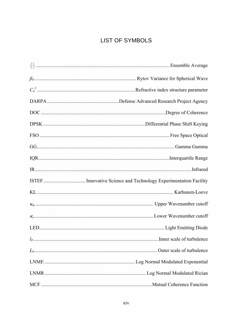
LIST OF SYMBOLS

⋅ ............................................................................................................ Ensemble Average

β0 .................................................................................. Rytov Variance for Spherical Wave

Cn2 ............................................................................... Refractive index structure parameter

DARPA .......................................................... Defense Advanced Research Project Agency

DOC ..................................................................................................... Degree of Coherence

DPSK .................................................................................. Differential Phase Shift Keying

FSO ......................................................................................................... Free Space Optical

GG ............................................................................................................... Gamma Gamma

IQR .......................................................................................................... Interquartile Range

IR............................................................................................................................... Infrared

ISTEF .................................. Innovative Science and Technology Experimentation Facility

KL .............................................................................................................. Karhunen-Loeve

κm ............................................................................................... Upper Wavenumber cutoff

κo ................................................................................................ Lower Wavenumber cutoff

LED ..................................................................................................... Light Emitting Diode

l0 ..................................................................................................... Inner scale of turbulence

L0 ................................................................................................... Outer scale of turbulence

LNME ......................................................................... Log Normal Modulated Exponential

LNMR .................................................................................. Log Normal Modulated Rician

MCF .......................................................................................... Mutual Coherence Function

xv

MLCD ................................................................ Mars Laser Communication Development

MTF ...................................................................................... Modulation Transfer Function

OOK .............................................................................................................. On-Off Keying

PDF ......................................................................................... Probability Density Function

ρc .............................................................................................................. Correlation Width

ρ0 .................................................................................................. Spatial Coherence Radius

RMS ......................................................................................................... Root Mean Square

SNR ..................................................................................................... Signal to Noise Ratio

WSF .............................................................................................. Wave Structure Function

1

1 INTRODUCTION

July 7, 1960 Maiman stimulated the emission of coherent light from a ruby rod. Shortly after,

his assistant joked he had created “a solution looking for a problem.” Since then many uses for

the laser have come about in physics, chemistry, medicine, military and the communications

industry. The laser’s unique ability to generate coherent light made it extraordinary.

Preceding optical fibers, confocal optical waveguides were used to mitigate long distance

propagation of light. The waveguides incorporated regularly spaced heaters causing the air to act

as a lens and focus the light. This concept was adopted from millimeter wave transmission, but

proved to be unsuccessful. In 1970 two key demonstrations took place: continuous laser

emission from a semiconductor at room temperature and a low-loss glass optical fiber.

Development of these technologies led to the telecommunications boom in the 1980’s. Data

rates of 2.5Gbps were achieved over a fiber, equating to 32,000 simultaneous phone

conversations. In 1988 the first fiber optic cable was laid across the Atlantic Ocean. The

development of erbium-doped amplifiers created a means of direct optical amplification of the

optical signal within the fiber, thereby eliminating the optical-to-electrical conversion process

previously required for signal amplification. The erbium-doped amplifier provided amplification

across a broad band of wavelengths, and was a natural fit for wavelength-division multiplexing;

the standard in today’s telecommunications [1].

2

In the mid-1960’s NASA tested laser transmission from the earth to the Gemini space capsule

with mixed results. As technology matured with the development of pointing and tracking

systems, space based laser communications became more realizable. In 2010, NASA had

planned to test the first deep space laser communication link under the Mars Laser

Communication Development (MLCD) program [2]. The system promised to communicate

nearly ten times faster than any existing radio link. However, budgetary issues in 2005

postponed the program. Outer space is an ideal medium to propagate light through; unlike earth,

it is nearly a vacuum and there are no atmospheric obstacles.

Free space optical communications (FSOC) is becoming more of a commonplace. Technologies

are advancing the use of LEDs indoor as combined lighting and short-range optical

communication. Atmospheric models for propagation through turbulence have matured over the

past fifty years since Tatarskii’s pioneering work [3, 4]. The electronics required to transmit and

receive optical signals are shrinking and becoming more efficient due to advances in

semiconductors. Point-to-point long-range FSOC has been advancing thanks to government

(DARPA) funded programs such as THOR, ORCLE, IRONT-2, and ORCA [5]. Ultraviolet

radios take advantage of the scattering at short wavelengths to create a secure short-range

channel with high signal to noise ratio (SNR). All major FSOC programs to this date have been

based upon intensity modulation schemes; on-off keying (OOK), or more recently binary pulse-

position modulation (BPPM). Future FSOC systems will take advantage of the signal gain and

SNR improvements from a coherent detection system, i.e. amplitude and phase detection.

3

Optical frequencies allow for higher bandwidth, faster data rates, smaller antennas, smaller size

and weight of components, increased directivity of EM radiation, and increased security. An

FSO communication system has the advantage to be deployed in situations where a fiber optic

cable is not practical. In the situation of a disaster site, FSO communication systems could be

quickly deployed and provide high bandwidth communications. However, at the short

wavelengths of optical waves, problems arise that are not a concern with RF communication.

The earth’s atmosphere has three main hurdles to overcome when using it as a communication

channel; absorption, scattering, and turbulence. Absorption of optical waves results in

attenuation, it occurs throughout the visible and IR spectrum. Absorption is a selective process

and results from specific molecules in the atmosphere having an absorption band at an optical

wavelength. Scattering occurs when a particle in the atmosphere is on the same order of

magnitude of the optical wavelength [6, 7]. The interaction of the particle and light wave causes

an angular redistribution of a portion of the radiated wave. Optical turbulence is a result of

fluctuations in the index of refraction along a propagation path. These fluctuations distort the

phase front and vary the temporal intensity of an optical wave. The combination of these

atmospheric effects on an optical system can cause phenomena such as beam spreading, image

dancing, beam wander, and scintillation [7].

The dominant noise source in an FSO communication system is atmosphere-induced intensity

and phase fluctuations; scintillation. A larger aperture (collecting lens) can help reduce

scintillation effects and improve SNR. Design criteria such as detector threshold level,

probability of detection, mean fade time, number of fades, and SNR require knowledge of the

4

probability density function (PDF) of the received irradiance of the optical field. The PDF of the

received irradiance is nonstationary by nature and is dependent upon the atmospheric turbulence

parameters, transmitted beam characteristics, and receiver design parameters; such as aperture

size and bandwidth. Nonetheless, an accurate PDF of the received irradiance is necessary to

build a robust and reliable FSOC.

5

2 BACKGROUND

2.1 Random Processes

Any set of data collected from a physical phenomenon can be classified as either deterministic or

nondeterministic. A deterministic data set can be explicitly described by a mathematical

formula. In a deterministic system, a repeated set of given initial conditions will always result in

the same output. However, there is no way to predict the exact value of a nondeterministic

phenomenon at an instant in time. Thereby these data are random by nature and can only be

described by means of probability statements and statistical averages [8]. Any detection system

in real life experiences noise and therefore requires a probabilistic treatment.

2.1.1 Stationarity, homogeneity, isotropy, and ergodicity

A stationary process has moments invariant with translations in time [9]. In nature, truly

stationary processes do not exist because there typically exists some stop time for the process [7,

10]. In some applications the random process does not change significantly over a finite sample

time and thus can be considered a stationary process. The condition of strict stationarity implies

all joint density functions of all orders describing the process to be independent of time. A more

relaxed and commonly used condition is stationarity in a wide-sense. A process is considered

6

wide-sense stationary if the first and second moments do not vary with time [7, 9]. In practice, a

finite sample of a random phenomenon is typically used to represent the process [8, 11]. The

entire sample may not be wide-sense stationary, but parts of it might be. In this case, stationary

increments of the sample can be used to calculate statistics of the process.

Random functions of a vector spatial variable, ( )zyx ,,R , and possibly time are called random

fields [7]. The concept of homogeneity is introduced when considering spatial statistics. A

random field is said to be homogeneous if the moments are invariant under a spatial translations.

A stationary random process in time is analogous to a homogeneous random field in space.

Isotropy is defined as uniform in all directions and therefore an isotropic field has no preferred

direction for statistics, all average functions describing the statistics of the field remain

unchanged regardless of a rotation in the coordinate system [10].

A process is called ergodic if the time or space average is equivalent to the ensemble average

[10]. Note that only stationary processes can be ergodic [8]. For an ergodic process, the

statistics of the random process, such as the density functions and moments, can be determined

from a single time sample.

Most experimental data of interest is fundamentally nonstationary; examples include ocean

waves, atmospheric turbulence, and economic time-series data [8]. The assumptions of

stationarity, homogeneity, isotropy, and ergodicity are necessary to apply any of the available

turbulence theory. Unfortunately, atmospheric turbulence is a nonstationary process and caution

must be taken when analyzing data records.

7

2.1.1.1 Testing for stationarity

Many procedures exist to test a time series data set for stationarity. The test procedures fall into

two main categories, parametric and nonparametric. Parametric tests assume a known

distribution of the data, they are more powerful, and generally require less data than

nonparametric tests to reach a conclusion. Nonparametric tests are commonly used and more

widely applicable because they require no assumption regarding the underlying nature of the

data. Consequently, they are less powerful than parametric tests [12]. Examples of parametric

tests are the Chi-squared and Kolmogorov-Smirnoff goodness-of-fit tests. Examples of

nonparametric tests are the sign test, Wilcoxon signed-rank test, runs test, and reverse

arrangements test [8, 12].

In order to test a random data set for stationarity, it must be assumed the data record will

properly reflect the nonstationary character of the random process in question. Also, the data

record needs to be significantly longer compared to the lowest frequency component in the data.

Under the previous two assumptions a single data record over time can be investigated. First, the

sample record is divided into N equal time intervals where the data in each interval may be

considered independent. Second, the mean square value is computed for each of the N intervals.

Those N mean square values are then subjected to any of the nonparametric tests. Bendat and

Piersol outline the application of the reverse arrangements test for stationarity [8].

8

For the reverse arragements test, we can write the N mean square values as Nixi ,...,3,2,1, = .

The number of times ji xx > is counted for ji > , each inequality is called a reverse arrangement.

The general definition for the number of reverse arrangements in a data record, A, is [8]

∑−

==

1

1

N

iiAA , (1)

where

∑+=

=N

ijjii hA

1 (2)

and

⎩⎨⎧ >

=otherwise

xxifh ji

ji 0

1. (3)

Assuming the N observations are independent, then the number of reverse arrangements is a

random variable A with mean and variance defined by Aμ and 2Aσ , respectively [8]

( )4

1−=

NNAμ (4)

9

( )( )72

15272

532 232 −+

=−+

=NNNNNN

Aσ . (5)

If the number of reverse arrangements is close to the mean value, then the sample of random data

is considered stationary.

To formally define upper and lower bounds based upon a specific level of significance, the z-

score is used. If we always assume a level of significance of 5% then the upper and lower

bounds are approximately defined by two standard deviations of the mean number of reverse

arrangements, [13]

AA

AA

boundlowerboundupper

σμσμ

22

−=+=

. (6)

If the mean number of arrangements A lies within the bounds defined above, we can say with a

95% confidence level the data is stationary over the prescribed time interval.

2.1.2 Probability density function

The quantity observed in a trial of an experiment is a random variable. A random variable is a

rule that assigns every outcome of an experiment a number. The random variable is a function

mapping the set of outcomes to a set of numbers. Similarly, a random process is a function that

10

maps each outcome of an experiment to a function. A random process observed at a discrete

point in time is a random variable. A random process is usually treated as a function of time, but

can also be a function of space. [7-9]

A probability distribution for a random variable organizes the probabilities observed in an

experiment. The distribution defines the range and probability of values a random variable can

attain. The probability density function of a random variable describes the density of probability

at each point within the sample space. The PDF is often displayed as a graph with the sample

value on the abscissa and the corresponding probability on the ordinate. An estimate of the PDF

of a random variable or process can be created from a sample data record through the use of a

histogram with sufficiently small bins. [7-9]

If a random process is sampled a finite number of times, then a collection of random variables is

obtained. Since each time sample of a random process is a random variable, then a random

process has a collection of PDFs described by the joint PDF of order n [7],

( );,;;,;, 2211 nnx txtxtxp K . (7)

In general, the complete joint PDF is required to describe a random process. However, under the

assumption of a stationary and ergodic random process, the PDF of a single time sample is

sufficient.

One of the fundamental properties of all PDFs is [14]

11

( )∫∞

∞−

= 1dxxfx , (8)

i.e. the total area under a PDF is unity. The cumulative distribution function (CDF) can be

derived from the PDF through integration [14]

( ) ( )∫∞−

=x

duufxF xx , (9)

where u is a dummy variable of integration. To calculate the probability of an event being within

an interval (a,b) from a continuous random variable, the PDF is integrated over an interval [14]

( ) ( )dxxfbab

a∫=<< xxPr . (10)

Often the conditional probability density function of a random variable is known and the

unconditional density is of interest. The relationship between the unconditional density

( )yxf ,yx and the conditional densities ( )yxf =yx | and ( )xyf =xy | is [14]

( ) ( ) ( ) ( ) ( )xfxyfyfyxfyxf xyyxyx xy ==== ||, , (11)

12

where Bayes’ theorem has been used relate the conditional densities and the marginal densities

of each random variable, ( )yfy and ( )xfx . The total probability for x can be written by

removing the condition y=y , this is done by taking the average of the conditional PDF over

marginal PDF of y [14]

( ) ( ) ( )∫∞

∞−== dyyfyxfxf yxx y| , (12)

and similarly for y

( ) ( ) ( )∫∞

∞−== dxxfxyfyf xyy x| . (13)

As stated earlier, the PDF of a nonstationary process changes with time. Time-averaging of a

nonstationary process will generally produce a severely distorted PDF [8]. Computing the PDF

from a data sample with a nonstationary second moment will tend to exaggerate the probability

density in the tails (high and low values) at the expense of intermediate values [8]. However,

these distortions can be reduced by the selection of stationary increments within the finite

sample.

13

2.1.2.1 Histogram

A histogram is a statistical tool for displaying frequency of events. The x-axis represents the

data of interest and the y-axis represents how frequent the data occur over a specified non-

overlapping interval, called a bin. A histogram represents numbers by area and is often

displayed with a bar chart [15]. The bin widths of a histogram are typically of equal width,

however, some data sets benefit from unequal bin widths. A PDF of the data can be estimated

from a histogram with equal bin widths by normalizing the total area of the histogram to unity

[8]

( )NWN

xp x=ˆ , (14)

where N is the total number of data points, W is the bin width centered at x, and xN is the number

of data values (bin height) within the range 2Wx ± . A PDF of the data can also be estimated

for unequal bin widths. For a histogram, the sum of the heights of each bin is equal to the total

number of data points,

NNbinsall

x =∑ . (15)

14

First, consider creating a histogram in two parts, A and B, where A is the lower part of the

histogram up to some arbitrary value and B is the remainder of the histogram. If the bins for

parts A and B were equal, BA WW = their histograms would be

( )NW

Nxp

A

AxequalA

,,ˆ = , (16)

( )NW

NNW

Nxp

A

Bx

B

BxequalB

,,,ˆ == . (17)

If two different bin widths were considered, AW and BW , where BA WW < then the heights of the

bins in part B would need to be normalized to the area of the bins in part A [15],

B

AequalBxunequalBx W

WNN ,,,, → . (18)

Their histograms for unequal bin widths would then be

( )NW

Nxp

A

AxunequalA

,,ˆ = (19)

( )NW

Nxp

B

BxunequalB

,,ˆ = (20)

15

When plotted on the same graph with their corresponding bin widths the partial histograms of A

and B combine to display the PDF of the entire data set.

Selecting the proper bin size is essential when generating a histogram. If the bin size is too large

important details will be smoothed out, if the bin size is too small the histogram will be jagged

and the trend indiscernible. Several techniques exist for determining bin sizes based upon a

given set of data. Two methods in particular are based upon minimizing the mean square error

and are robust enough to support data sets of any size and range. Scott’s rule [16] defines the

optimal bin size width, h, from the standard deviation of the data σ and the number of samples

n,

31

5.3n

h σ= . (21)

Freedman and Diaconis [17] define the optimal bin size from the interquartile range (IQR), a

measure of statistical dispersion, and the number of samples n,

31

*2nIQRh = . (22)

16

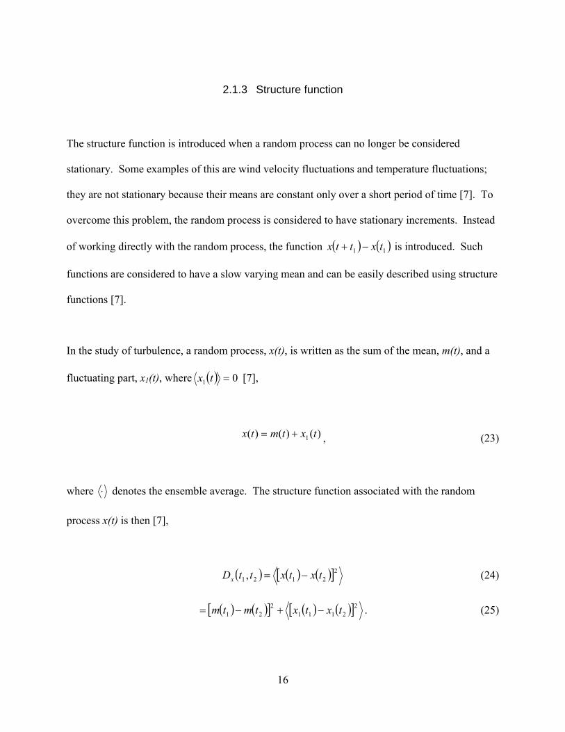
2.1.3 Structure function

The structure function is introduced when a random process can no longer be considered

stationary. Some examples of this are wind velocity fluctuations and temperature fluctuations;

they are not stationary because their means are constant only over a short period of time [7]. To

overcome this problem, the random process is considered to have stationary increments. Instead

of working directly with the random process, the function ( ) ( )11 txttx −+ is introduced. Such

functions are considered to have a slow varying mean and can be easily described using structure

functions [7].

In the study of turbulence, a random process, x(t), is written as the sum of the mean, m(t), and a

fluctuating part, x1(t), where ( ) 01 =tx [7],

)()()( 1 txtmtx += , (23)

where ⋅ denotes the ensemble average. The structure function associated with the random

process x(t) is then [7],

( ) ( ) ( )[ ]22121 , txtxttDx −= (24)

( ) ( )[ ] ( ) ( )[ ]221112

21 txtxtmtm −+−= . (25)

17

It is important to note that if the mean is slowly varying then ( ) ( )21 tmtm ≅ for 1t “close” to 2t

the first term reduces to zero and the structure function is approximated by [7],

( ) ( ) ( )[ ]2211121 , txtxttDx −≅ . (26)

This concept can be easily extended into the spatial domain. As discussed in a previous section,

the spatial equivalent to stationary increments is locally homogeneous. This allows a random

field to be written in the spatial domain as

( ) ( ) ( )RRR 1xmx += , (27)

where R a position vector in space. Applying the same concept used for a random process with

stationary increments, the structure function for a local homogeneity random field can be written

as

( ) ( ) ( ) ( )[ ]21121 , RRRRRR +−== xxDD xx . (28)

18

2.1.4 Averaging time

There are three types of averaging: space, time, and ensemble. Space averaging is sampling a

group of processes over a prescribed area at a particular instant [10]. Time averaging is

sampling a single process for a sufficiently long realization. Ensemble averaging is sampling a

group of identical processes at a particular instant. In practice, the ensemble average is rarely

available and space and time averages are typically used [10].

A random process observed in real life is never completely homogenous or stationary. The best

one can do is require that the variance falls to an acceptably small value over sufficiently large

integrating times. It is difficult to measure the ensemble average of a random process. Instead,

the assumption of ergodicity is made and thus the time or space average is equivalent.

When calculating higher order moments from experimental data, care must be taken to avoid

detector saturation as well as assure a sufficient data sample. Higher order moments require a

longer sample record than lower order moments to retain the same accuracy of lower order

moments. For instance, the fourth moment weighs the extreme tails of the distribution much

more heavily than lower order moments because it is looking at values occurring less frequently.

As an example take a zero mean Gaussian process, the sample time required to determine the

fourth moment with the same accuracy as the second moment is more than five times as long

[10]. The necessary averaging, or sample, time must be considered when recording data,

especially non-stationary data.

19

3 ATMOSPHERIC TURBULENCE

Classically, turbulence is derived from fluid dynamics. Dynamic mixing distinguishes turbulent

flow from laminar, or smooth, flow. The Reynolds number defines a dimensionless ratio

between inertial and viscous forces within a flow. Low Reynolds numbers characterize laminar

flow where viscous forces dominate and the motion is smooth. High Reynolds numbers

characterize turbulent flow where inertial forces dominate and the formation of random eddies

and vortices occur [7, 10, 18].

Atmospheric turbulence is analogous to turbulence in a fluid; in the atmosphere the air is

considered the fluid. The term atmospheric turbulence encompasses variations in wind, pressure,

and temperature. A subset of atmospheric turbulence is optical turbulence, i.e. turbulence having

a strong effect at optical wavelengths. Optical turbulence is defined as small random

fluctuations in the refractive index of air. Solar heating creates a temperature gradient between

the ground and the air. The temperature gradients cause the pressure of the air to change which

causes the refractive index differences, this is optical turbulence.

3.1 Solution Techniques for the Stochastic Helmholtz Equation

Fundamentally, a propagating wave is governed by the wave equation. Assuming the time and

space components of the wave function are separable, the Helmholtz equation results. An optical

20

wave propagating through an unbounded continuous medium with a smoothly varying refractive

index obeys the stochastic Helomholtz equation [7]

( ) 0222 =+∇ UnkU R (29)

where U is the complex amplitude of the field, 2∇ is the Laplacian operator, λπ2=k is the

wavenumber, and ( )R2n is the index of refraction in three dimensions. It is assumed the

variations in the refractive index are slow compared to the frequency of the optical wave. The

random refractive index creates a nonlinear stochastic partial differential equation, which to this

day has no closed form solution [19]. There are several classic methods for approximately

solving (29). Under weak or strong fluctuation conditions, as defined by the Rytov variance in

section 3.9.1, both the parabolic equation method and the extended Huygens-Fresnel principle

yield approximations to the first and second order moments of U, the latter method lending itself

to spherical waves [7]. Under weak fluctuations two perturbation methods are commonly used,

the Born approximation and the Rytov approximation [7]. The Born approximation writes the

complex amplitude of the field as a sum of perturbations, while the Rytov approximation

assumes a multiplication of exponential perturbation functions [7]. The Born approximation is

limited to very short propagation distances and is not useful for most applications of optical

wave propagation [7]. The Rytov approximation has fewer limitations and is the most

widespread method used to solve the stochastic Helmholtz equation. Early work focused only on

the first-order perturbation [3, 4], while later work demonstrated a need for the second-order

term to calculate statistical moments of the optical field [7, 20].

21

3.2 Refractive Index Structure Parameter, Cn2

Physically, the refractive-index structure parameter, Cn2, is a measure of the strength of the

fluctuations in the refractive index. The index of refraction of a medium is important when

propagating light through it. The atmosphere exhibits random fluctuations in refractive index as

the temperature and wind speed change. At a point R in space and time t, the index of refraction

can be mathematically expressed as [7]

( ) ( )tnntn ,, 10 RR += , (30)

where ( ) 1,0 ≅= tnn R is the mean value of the index of refraction and ( )tn ,1 R represents the

random deviation of ( )tn ,R from its mean value; thus we take, ( ) 0,1 =tn R . Typically time

variations of the refractive index are slow compared to the frequency of the optical wave;

therefore the wave is assumed to be monochromatic. The expression in (30) can then be written

as [7]

( ) ( )RR 11 nn += , (31)

where ( )Rn has been normalized by its mean value n0.

The index of refraction for the atmosphere can be written for visible and IR wavelengths as [7]

22

( ) ( ) ( )

( )RRR

TPn 236 1052.71106.771 −−− ×+×+= λ

, (32)

where λ, the optical wavelength, is expressed in μm, P(R) is the pressure in millibars at a point

in space, and T(R) is the temperature in Kelvin at a point in space. Since the wavelength

dependence for optical frequencies is very small; (32) can then be rewritten as [7]

( ) ( )

( )RRR

TPn 610791 −×+≅

. (33)

Since pressure fluctuations are usually negligible, the index of refraction exhibits an inverse

relation with the random temperature fluctuations. This simple approximation only holds in the

visible and near-IR regime. Extending the wavelength into the far-IR introduces other issues

such as humidity.

Since ( ) 0,1 =tn R is assumed, the spatial covariance ( )21 , RRnB of n(R) can be expressed as

[7]

( ) ( ) ( ) ( )RRRRRRRR +=+= 11111121 ,, nnBB nn . (34)

If the random field is both statistically homogeneous and isotropic, the spatial covariance

function can be expressed in terms of a scalar distance 12 RR −=R . Assuming statistically

23

homogeneous and isotropic turbulence, the related structure function exhibits asymptotic

behavior [7]

( )

⎪⎩

⎪⎨⎧

<<

<<<<=

−0

23/40

200

3/22

,

,

lRRlC

LRlRCRD

n

nn

, (35)

where Cn2 is the index-of-refraction structure parameter, l0 is the inner scale of turbulence, and L0

is the outer scale of turbulence. The inner and outer scales of turbulence act as a lower and upper

bound, respectively, for the fluctuations of the refractive index. Behavior of Cn2 at a point along

the propagation path can be deduced from the temperature structure function obtained from point

measurements of the mean-square temperature differences in two fine wire thermometers. With

the use of (33), [7]

2

2

262 1079 Tn C

TPC ⎟⎠⎞

⎜⎝⎛ ×= −

. (36)

Typical values for Cn2 are between 10-16 32−m for weak fluctuations and 10-12 32−m for strong

fluctuations. Figure 1 illustrates the behavior of Cn2 throughout a typical day. The data was

taken using a commercial scintillometer at the Innovative Science and Technology

Experimentation Facility (ISTEF) laser range. When there is no sunshine, Cn2 is low. As the sun

begins to rise, Cn2 increases until it reaches a maximum in the middle of the day. As the sun

begins to set, Cn2 decreases. An interesting trend to note on the plot is the dip in Cn

2 before and

24

after sunrise. These two dips are called the quiescent periods. This drop in Cn2 occurs due to the

temperature gradient between the ground and atmosphere being minimal.

1.0E-14

2.1E-13

4.1E-13

6.1E-13

8.1E-13

1.0E-12

0:00 2:00 4:00 6:00 8:00 10:52 13:24 15:26 17:26 19:26 21:26 23:26

Time

Cn^2

(m^-

2/3)

Figure 1: 24-hour Cn

2 profile of data taken over a 1km terrestrial path during the summer in Florida.

3.3 Power Spectrum Models

The Riemann-Stieltjes integral allows the covariance (or correlation) function of a random

process to be associated with a corresponding power spectrum. Through this relationship, the

covariance function is the Fourier transform of the power spectrum and thus they are transform

pairs [7],

Cn2 (m

-2/3

)

25

( ) ( )∫∞

∞−

= ωωτ τω dSeB xi

x (37)

( ) ( )∫∞

∞−

−= ττπ

ω τω dBeS xi

x 21 (38)

where ω represents angular frequency, τ represents time, ( )τxB is the covariance function, and

( )ωxS is the power spectrum. These general transform relations are know as the Wiener-

Khintchine theorem [7].

For theoretical work, the three-dimensional power spectrum is required. Using the Riemann-

Stieltjes integral a relationship between the three-dimensional power spectrum and the

covariance function for a statistically homogeneous complex random field can be written as [7]

( ) ( )∫ ∫ ∫∞

∞−

•−⎟⎟⎠

⎞⎜⎜⎝

⎛=Φ RdBe u

iu

33

21 RK RK

π (39)

where ( )zyxK κκκ ,,= is the vector wave number in [rad/m] and ( )zyx ,,=R is the spatial

position vector. The equation simplifies when the random field is both homogeneous and

isotropic and thus spherical symmetry can be assumed [7],

( ) ( ) ( )∫∞

==Φ0

2 sin2

1 dRRRRBuu κκπ

κ . (40)

26

where K=κ is the magnitude of the wave number vector and R=R .

For work in atmospheric turbulence, the three-dimensional spatial power spectrum of the

refractive index is of interest. The inverse Fourier transform of (40) yields the covariance

function for the refractive index fluctuations [7],

( ) ( ) ( )∫∞

Φ=0

sin4 κκκκπ dRR

RB nn (41)

where the subscript u has been replaced with n to denote the refractive index. Using the

relationship between the refractive index structure function and covariance, the relation between

the spectrum and the structure function is [7]

( ) ( ) ( )[ ]

( ) ( )∫∞

⎟⎟⎠

⎞⎜⎜⎝

⎛−Φ=

−=

0

2 sin18

02

κκκκκπ dR

R

RBBRD

n

nnn

. (42)

The Kolmogorov power-law spectrum can be deduced from the structure function in (35) [7],

( ) 003112 11,033.0 lLCnn <<<<=Φ − κκκ , (43)

it represents the power spectral density for the refractive index fluctuations over the inertial

subrange, 00 11 lL <<<< κ . The Kolmogorov spectrum is the most commonly used power

27

spectrum in optical turbulence calculations predominantly due to its simplicity. It is only valid

within the inertial subrange, however it can be extended to represent all wavenumbers by

assuming an infinite outer scale ( ∞=0L ) and a zero inner scale ( 00 =l ) [7].

Several other power spectrum models have been introduced based upon the 2/3 structure

function. These other models include the effects of a finite inner and/or outer scale on the power

spectrum. Tatarskii included inner scale effects by truncating the power spectrum at high

wavenumbers (the dissipation range) with a Gaussian shaped function [7],

( ) 002

23112 92.5;1,exp033.0 lLC m

mnn =>>⎟⎟

⎠

⎞⎜⎜⎝

⎛−=Φ − κκκκκκ . (44)

Von Kármán included outer scale effects by truncating the power spectrum at low wavenumbers

[7]. The von Kármán spectrum was later combined with the Tatarskii spectrum to incorporate

both inner and outer scale effects and thus be valid over all wavenumbers; the spectrum was

named the modified von Kármán [7].

( ) ( )( )

( )⎪⎪

⎩

⎪⎪

⎨

⎧

=∞<≤+

−

<<≤+

=Φ

061120

2

222

061120

2

2

92.5;0,exp

033.0

10,033.0

lC

lC

mm

n

n

n

κκκκ

κκ

κκκ

κ , (45)

28

where 00 Lc=κ and c is a constant typically assuming a value of 1 or π2 , the upper expression

is the von Kármán and the lower expression is the modified version.

The above power spectrum models only have correct behavior within the inertial subrange and

do not incorporate the bump occurring at higher wavenumbers near 01 l [7]. Hill and Clifford

first formulated a modified power spectrum for temperature fluctuations to incorporate the bump

at higher wavenumbers, they also verified the bump in the spectrum through experimental

temperature data [21]. Andrews developed a more tractable analytic expression to Hill’s

modified spectrum for refractive index fluctuations, including an outer scale parameter, it is

referred to as the modified atmospheric spectrum [7, 21],

( ) ( )

( )0

61120

2

22672

3.3;0

exp254.0802.11033.0

l

C

l

l

llnn

=∞<≤

+

−

⎥⎥⎦

⎤

⎢⎢⎣

⎡⎟⎟⎠

⎞⎜⎜⎝

⎛−⎟⎟

⎠

⎞⎜⎜⎝

⎛+=Φ

κκ

κκ

κκκκ

κκκ

, (46)

where 00 Lc=κ and c is a constant typically assuming a value of 1 or π2 . The terms within

the brackets account for the bump at high wavenumbers [7].

3.4 Turbulence Generation

Generally speaking, a turbulent eddy is a structured glob of fluid within the bulk fluid mass

having a specific life history. Eddy size is defined by the outer scale L0 and inner scale l0 of

29

turbulence. The outer scale defines the largest eddy size, while the inner scale defines the

smallest eddy size. All eddy sizes laying between the inner and outer scales make up the inertial

subrange. When the power spectrum of eddies is considered, wavenumbers are typically used.

The wavenumber is defined as

λπ2

=k , (47)

where λ is the wavelength or diameter of the eddy. For the Kolmogorov spectrum within the

inertial subrange, the three-dimensional power spectral density has a slope of -11/3 (43).

For a high Reynolds number, i.e. strong mixing, the generation of the atmospheric turbulence

spectrum can be described as follows [10]. Under stable conditions, energy is fed from the wind

shear into the temperature gradient. At low wavenumbers, the spectrum is anisotropic.

Distortion of the large eddies by inertia forces, caused by fluctuating velocity gradients, transfer

energy from the low wavenumber portion of the anisotropic spectrum to higher wavenumbers.

At increasing wavenumbers, feeding deteriorates and the spectrum becomes more isotropic due

to pressure forces. The spectrum is considered isotropic in the ranges of inertial transfer and

dissipation. The range of wavenumbers where no significant feeding or dissipation is occurring,

only inertial transfer of energy, defines the inertial subrange. At large enough wavenumbers

dissipation transpires, during which molecular action destroys eddy structure. Heat is neither

gained or lost as a parcel of air is swirled into an eddy, this is because turbulence mixing of air is

an adiabatic process [18]. Figure 2 illustrates the roles of solar heating (convective energy) and

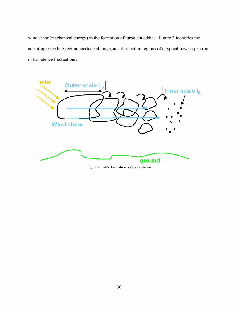
30

wind shear (mechanical energy) in the formation of turbulent eddies. Figure 3 identifies the

anisotropic feeding region, inertial subrange, and dissipation regions of a typical power spectrum

of turbulence fluctuations.

Figure 2: Eddy formation and breakdown.

31

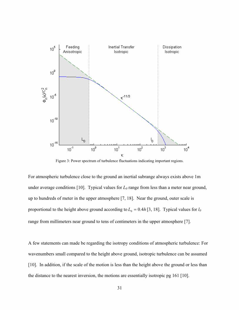
Figure 3: Power spectrum of turbulence fluctuations indicating important regions.

For atmospheric turbulence close to the ground an inertial subrange always exists above 1m

under average conditions [10]. Typical values for L0 range from less than a meter near ground,

up to hundreds of meter in the upper atmosphere [7, 18]. Near the ground, outer scale is

proportional to the height above ground according to hL 4.00 = [3, 18]. Typical values for l0

range from millimeters near ground to tens of centimeters in the upper atmosphere [7].

A few statements can made be regarding the isotropy conditions of atmospheric turbulence: For

wavenumbers small compared to the height above ground, isotropic turbulence can be assumed

[10]. In addition, if the scale of the motion is less than the height above the ground or less than

the distance to the nearest inversion, the motions are essentially isotropic pg 161 [10].

32

Mechanical eddies of smaller wavelengths are more isotropic than eddies produced by heating

and transfer little momentum. However, heat is transported more efficiently through larger

eddies pg 109 [10].

There are four general regions in the atmosphere where the turbulence is expected to be high:

Near the ground, in convective clouds, in the surrounding region of jet streams and sharp

troughs, and in the air flow on the lee of mountains. Close to the ground, the strength of

turbulence is predominantly a function of the height above ground, ground roughness, and wind

shear. The conditions of the surrounding environment contribute differently to each of the three

components of motion in the atmosphere. Fluctuations in vertical motion near the ground are

governed by wind speed and surface roughness. Fluctuations in lateral motion are governed by

wind speed. Fluctuations in longitudinal motion near the ground are governed by wind speed

especially over rough terrain. The temperature fluctuations, which drive the refractive index

fluctuations, are produced by vertical velocity fluctuations. In general, wind blowing over a

rough surface, such as the ground, creates mechanical turbulence.

3.4.1 Birth of an eddy

Temperature gradients between the hot ground and the cool air form local unstable air masses.

The sunlight passes through the air with out heating it too much. The sunlight heats the ground

and the ground reradiates the heat due to its low heat capacity. The hot air then rises in the

33

presence of surrounding cold air in the form of plumes. The wind shears the rising blob of hot

air from the ground and a turbulent eddy is formed. The temperature difference causes a density

difference which drives the change in refractive index. As the eddy rises it cools from the

surrounding air and expands adiabatically [18] while the wind continuously breaks the large

turbulent cell into smaller ones. The expansion causes the density difference to decrease thus

reducing the effectiveness of the eddy and eventually the eddy dissipates.

3.5 Thermal Plumes and Near Ground Effects (Near-Ground Cn2 Fluctuations)

During the day and within the first few kilometers of the atmosphere (surface layer) the

temperature fluctuations, i.e., optical turbulence, are statistically non-stationary and

inhomogeneous. Time records of temperature fluctuations, measured at a fixed location with a

fine wire temperature sensor, show a pattern of “bursty” fluctuations with intervening periods of

cooler air devoid of temperature fluctuation [22, 23]. These bursts are created by uneven heating

of the ground, warming the air and its subsequent rising due to buoyancy forces. The spatial

extent of the plumes may be tens of meters. This rising air creates plumes of optical turbulence,

and, as the plumes rise, the higher cooler non-turbulent air sinks. Measurements show that these

optical turbulence plumes can rise up to 200 meters [22]. Figure 4 shows such typical heat

plumes forming in a fluid from a heated surface, rising due to buoyancy, and subsequently

breaking into regions of strong turbulence. Optical turbulence has a similar structure and

behavior.

34

Figure 4: Images of thermal plumes rising from a heated surface in a fluid [24]. Mechanical and inertial forces

break the plumes apart as they rise.

In the atmosphere, the optical turbulence rises and the air cools with the decreasing temperature

gradient above the earth’s surface, thereby reducing the optical turbulence. Additional

reductions in optical turbulence occur indirectly from increased humidity. The convection and

thermal pluming is reduced by the presence of ground moisture since part of the sun’s heating is

used for evaporation instead of thermal pluming [18]. In the daytime, optical turbulence is

strongest near the ground, characterized by Cn2 on the order of 10-14 to near 10-12 m-2/3. During

this period the air temperature gradient is negative, and, with increasing altitude, it has been

observed that Cn2 often decreases from the surface layer with a h−4/3 altitude dependence [25],

where h denotes altitude above ground.

35

At night, the Earth’s surface cools by radiation and becomes colder than the air, producing more

stable conditions. This surface cooling produces a strong positive temperature gradient that can

reach tens or hundreds of meters or more. Within the temperature inversion, Cn2 will typically

increase with increasing wind speed up to around 4 m/s, and then decrease with stronger wind

speeds exceeding 4 m/s. Consequently, the decrease in Cn2 with altitude at nighttime does not

generally follow a h−4/3 altitude dependence; instead, similarity theory predicts the power-law

relation h−2/3 representing more stable conditions [25].

3.6 Taylor’s Frozen Turbulence Hypothesis

Taylor’s hypothesis states that the evolving structure of optical turbulence is slow compared to

the mean wind velocity [3]. Hence a propagating wave will pass through a spatially fixed

realization of turbulence. The movement of this fixed random media allows for comparison of a

wave propagating through a fixed media to measurements in the open atmosphere. If the

turbulence evolves during a measurement there is no obvious way to relate the calculated spatial

fluctuations to the temporal measurements.

Atmospheric parameters calculated from experimental measurements are typically determined

from temporal statistics, as opposed to spatial statistics. Under the assumption of Taylor’s

hypothesis, spatial statistics can be converted directly into temporal statistics with knowledge of

the average crosswind speed. The hypothesis assumes the spatial distribution of the turbulence

36

along the path is frozen and is moved across the observation path by the mean crosswind.

Similar to clouds moving in the sky, the structure of turbulence is assumed to evolve slowly with

respect to the crosswind speed. Therefore the speckle pattern produced by a laser beam

propagating through turbulence would not change structure, but simply move across an

observation plane in the direction of the mean crosswind. However, this assumption can not be

made when the component of the mean wind speed parallel to the propagation path dominates.

Under certain conditions, Taylor’s hypothesis can become suspect. We can denote ⊥v and ||v as

the perpendicular and parallel components of the average wind velocity, respectively. Since

fluctuations in the direction of the mean wind velocity are approximately 0.1, if ||1.0 vv ≈⊥ , then

the fluctuating portion of perpendicular component is of the same order as the mean [23]. In this

case, Taylor’s hypothesis does not hold. We can denote v and σ as the magnitude of the mean

wind speed and the standard deviation of the magnitude of the mean wind speed, ⊥σ as the

standard deviation of the perpendicular component of the wind speed, and α as the angle

between the wind direction and the direction of propagation. From Tatarskii’s turbulence theory

[3],

22

32σσ =⊥ (48)

we can then write [23]

ασσ

sin8.0

vv=

⊥

⊥ . (49)

37

Usually 1.0~vσ ; therefore for °= 90α , ~⊥⊥ vσ 10 percent. For °< 50~α , 1~>⊥⊥ vσ and

the validity of Taylor’s hypothesis becomes questionable [23].

3.7 Scale Sizes of Optical Turbulence

As a coherent optical wave propagates through optical turbulence, various eddies impress a

spatial phase fluctuation on the wave front with an imprint of the eddy scale size. The

accumulation of such phase fluctuations on the wavefront as the optical wave propagates leads to

a reduction in “smoothness” of the wavefront. Hence, the turbulent eddies further away from the

source experience a smoothness of the wavefront only on the order of the transverse spatial

coherence radius 0ρ . After a wave propagates a sufficient distance L, only those turbulent eddies

on the order of 0ρ or less are effective in producing further spreading and amplitude fluctuations

on the wave [7].

Under strong irradiance fluctuations the spatial coherence radius also identifies a related large-

scale eddy size near the source called the scattering disk 0ρkL . Basically, the scattering disk is

defined by the refractive cell size l at which the focusing angle Llf ~θ is equal to the average

scattering angle 01~ ρθ kD . That is, the field within a coherence area of size 0ρ at distance L

from the source is assumed to originate from a scattering disk 0ρkL near the source. Only

38

eddies equal to or larger than the scattering disk can contribute to the field within the coherence

area [7].

Only under weak fluctuations do all scale sizes affect a propagating wave. Under strong

fluctuations the propagating wave is affected by two distinct scale sizes; large-scale and small-

scale. Large-scale contributions are refractive and come from turbulent cells larger than the

Fresnel zone kL or the scattering disk, whichever is larger. Small-scale contributions to

scintillation are diffractive and come from turbulent cells smaller than the Fresnel zone or the

spatial coherence radius 0ρ , whichever is smallest. In the regime of weak turbulence, all scale

sizes contribute to scintillation and the Fresnel zone is the most important scale size [7]. Figure

5 shows the relationship of the cell sizes for an infinite plane wave.

39

Figure 5: Relevant turbulent eddy scale sizes for an unbounded plane wave with nm532=λ and

32132 105 −−×= mCn . The shaded region denotes scale sizes not contributing to scintillation under strong fluctuations.

3.8 Stochastic Field Properties

A stochastic field is an electromagnetic field random in both space and time. A sample of a

stochastic field is represented by a volume defined by some area of the field and some

observation time interval. For an optical wave propagating through atmospheric turbulence, this

space-time stochastic field can be considered a space-time narrow band fluctuation. That is, the

temporal characteristics of the optical field are slow compared to the temporal oscillation

40

frequency of the wave. Therefore the stochastic field can be represented by its complex

envelope. This section describes some techniques used when working with stochastic fields.

3.8.1 Second-order statistics

The mutual coherence function (MCF) is the second-order moment of the scalar complex

envelope of the optical field ( )LU ,r . It can be written as [7]

( ) ( ) ( ) ][,,,,, 221212 mWLULUL rrrr ∗=Γ (50)

where r1 and r2 are observation points in the receiver plane and L is the propagation distance

along the positive z-axis from the transmitter. All other second-order statistics of the optical

field stem from the MCF. The statistical quantities can be separated into two categories, those

dealing with the amplitude of the optical field and those dealing with the phase of the optical

field. The intensity, or irradiance of optical wave is given by the squared magnitude of the field

[7, 26]. Evaluating the MCF at identical observation points yields the mean irradiance [7]

( ) ( )LLI ,,, 2 rrr Γ= . (51)

For a finite beam the amplitude related quantities are the short and long term beam spot size as

well as beam wander. The short and long term beam spot sizes capture the additional beam

41

spread beyond diffraction due to turbulence. Beam wander describes the random steering of the

instantaneous center of the beam away from the optical axis in the plane of the receiver.

Although not investigated in this paper, the additional spreading of the beam due to turbulence

determines the loss of power at the receiver of an FSO system [7]. In addition, beam wander can

lead to intermittency as well as additional fluctuations of the signal especially for a beam

diameter on the order of the receiver.

The normalized MCF yields the degree of coherence (DOC), from which the wave structure

function (WSF) is derived. The DOC is written as [7]

( ) ( )

( ) ( )

( )⎥⎦⎤

⎢⎣⎡−=

ΓΓ

Γ=

LD

LLL

LDOC

,,21exp

,,,,,,

,,

21

222112

21221

rr

rrrrrr

rr, (52)

where ( )LD ,, 21 rr is the WSF. The separation distance 21 rr − at which the DOC falls to e1

defines the spatial coherence radius, 0ρ . The spatial coherence radius at the receiver describes

the loss of spatial coherence of an initially coherent beam due to turbulence [7]. The WSF is

written as

( ) ( ) ( )LDLDLD S ,,,,,, 212121 rrrrrr += χ (53)

42

and is the sum of the log-amplitude structure function ( )LD ,, 21 rrχ and the phase structure

function ( )LDS ,, 21 rr . The rms angle-of-arrival and rms image jitter are derived from the phase

structure function. Angle-of-arrival fluctuations in the optical wavefront in the plane of the

receiver cause jitter (dancing) of the image in the focal plane [7]. Random movement of the

image can cause blurred images as well as difficulty coupling light into a fiber.

3.8.2 Fourth-order statistics

Similar to second-order statistics, all fourth-order statistics emerge from the fourth-order cross-

coherence function, or the fourth moment of the optical field. The fourth moment is written as

[7]

( ) ( ) ( ) ( ) ( )LULULULUL ,,,,,,,, 432143214 rrrrrrrr ∗∗=Γ . (54)

It is seen from (50) that the mean irradiance is a second-order statistic. Therefore to examine

fluctuations in irradiance, fourth-order statistics must be studied. Unlike second-order statistics,

the phase is not a direct result of the fourth-order moment of the optical field [7]. This is because

the fourth moment of the optical field is looking at irradiance variations. However, phase

statistics such as phase variance, phase covariance function, phase structure function, and the

temporal phase spectrum can be inferred from the fourth moment [7]. The phase variance and

phase covariance function are nearly identical to their counterpart’s, scintillation index and

43

irradiance covariance and can therefore be derived from the fourth moment. It is important to

have knowledge of the phase statistics for coherent heterodyne receivers and phase modulation

techniques such as differential phase shift keying (DPSK) in an optical communications system

[7].

More importantly are the statistics of the irradiance fluctuations. The scintillation index,

irradiance covariance function, correlation width, and temporal irradiance spectrum can be

obtained directly from the fourth moment of the optical field [7]. The scintillation index

describes the irradiance fluctuations at a single point, while the irradiance covariance function

describes the correlation between irradiance at two points on the beam. Scintillation index is

vital in predicting the performance of an FSO communication system or a laser radar system.

The irradiance covariance function is used to determine the correlation width cρ associated with

irradiance fluctuations. The correlation width is commonly used to select an aperture size for a

receiver [7]. Aperture sizes on the order of cρ and smaller act like a point receiver, apertures

larger than cρ exhibit aperture averaging effects [7]. The correlation width is obtained by

normalizing the irradiance covariance function and evaluating it at the zero or 21 e crossing [7].

Invoking Taylor’s frozen turbulence hypothesis allows the calculation of temporal statistics from

the spatial irradiance statistics and the mean crosswind speed [7]. The temporal irradiance

function is one of the main characteristics of noise in an FSO communication system or a laser

radar system [7].

44

3.8.3 Coherence function of a stochastic field

The complex envelope of a stochastic field must be considered random at each point in time, t,

and space, r. Random fields are completely described by their probability density functions, i.e.

all higher order moments of the envelope. In practice it is unrealistic to have knowledge of all

higher order moments. Instead the random field is assumed to be wide-sense stationary and

analysis can then be confined to second-order statistics associated with the field; particularly the

coherence function. The time-space (mutual) coherence function of a stochastic field at points

( )11, rt and ( )22 , rt is [7, 26]

( ) ( ) ( )221122112 ,,,;, rrrr tUtUtt ∗=Γ , (55)

where denotes the ensemble average. A stochastic field is said to be coherence-separable if

its coherence function factors as [26]

( ) ( ) ( )212122112 ,,,;, rrrr st tttt ΓΓ=Γ , (56)

where the factor ( )21, rrsΓ is called the spatial coherence function and ( )21, tttΓ is called the

temporal coherence function of the field. The field is spatially homogeneous if the coherence

function depends only on the spatial distance 21 rr −=ρ . The field is temporally stationary if

the coherence function depends only on the time difference 21 tt −=τ [26]. Finally, a stochastic

45

field is completely homogeneous if it is both spatially homogeneous and temporally stationary.

A completely homogeneous coherence separable field is said to be spectrally pure and can be

written as [26]

( ) ( ) ( )ρτ sttt ΓΓ=Γ 22112 ,;, rr . (57)

3.8.4 Karhunen-Loeve expansion

A deterministic function can be expanded using a Fourier series representation, the coefficients

of the expansion are real numbers and the expansion basis consists of sinusoidal functions. The

Karhunen-Loeve (KL) expansion is for representing a stochastic process as a linear combination

of orthogonal functions, the coefficients are uncorrelated random variables and the orthogonal

set of the expansion basis depends on the covariance function of the stochastic process. Given a

stochastic electromagnetic field ( )tE ,r over a specific observation space-time volume defined

by [ ]Ttt +, and [ ]A , the expansion can be written as [26]

( ) ( )∑∞

==

0,,

ijj tatE rr φ (58)

where [26]

46

( ) ( ) rrr ddtttEa jA

Tt

tj ,, *φ∫ ∫

+

= . (59)

The random coefficients ja are the modal coefficients describing the power in the envelope in

each mode [26]. The functions ( )tj ,rφ form the complete set of orthogonal basis functions over

the space-time volume of the electromagnetic field [26]. The convergence of the series is in the

mean squared sense and requires bounded average energy in the field over the spatial area and

time interval of the series expansion. For a KL expansion the correlation function of the field

envelope and each member of the orthogonal function set satisfy the following integral relation

for some positive constants jγ [26]

( ) ( ) ( )12222112 ,,,;, tdtdttt jjA

Tt

tj 122 rrrrr φγφ =Γ∫ ∫

+

, (60)

this identifies the random coefficients ja as uncorrelated random variables and 2jj a=γ [26].

For a coherence separable field the left side of equation (60) reduces to [26],

( ) ( ) ( ) 222121 ,,, dtdtttA

Tt

tjst 22 rrrr∫ ∫

+

ΓΓ φ . (61)

The form of the equation shows that an eigenfunction solution always occurs as [26]

47

( ) ( ) ( )tgwt jjj rr1 =1,φ . (62)

jtjsj γγγ = (63)

where the terms above satisfy [26]

( ) ( ) ( )12221, tgdttgtt jjt

Tt

tjt γ=Γ∫

+

(64)

( ) ( ) ( )122 rrrrr jjsA

js wdw γ=Γ∫ 21, (65)

For a coherence separable field the temporal and spatial components are independent,

consequently the eigenfunctions and eigenvalues factor into a product of spatial and temporal

components. Therefore the eigenfunctions in (58) can be determined by from separate

calculations of the eigenfunctions for both the time and space coherence kernels in (64) and (65)

[26]. The KL expansion of a coherence separable field is then [26]

( ) ( ) ( )tgwEtE iji j

ji rr ∑∑= ,, (66)

where [26]

( ) ( ) ( ) rrr ddttgwtEE ijA

Tt

tji

**, ,∫ ∫

+

= (67)

48

The functions ( )tg j describe the temporal modes of the field over the time interval[ ]Ttt +,

while the functions ( )rjw describe the spatial modes of the field over the area A. The

corresponding itjs γγ eigenvalues are the mean square energy in each of these modes, i.e. 2, jiE .

Collecting the energy in all spatial and temporal modes yields the total average energy over the

space-time volume [26],

( )∫ ∫∑∑+∞

=

∞

==

A

Tt

ti jitjs ddttE rr 2

0 0,γγ . (68)

The total energy over the area during a particular time mode i is [26]

∑∞

=0jjsit γγ (69)

while the average energy over the time interval ( )Ttt +, in a particular spatial mode j is [26]

∑∞

=0iitjs γγ (70)

If the field is completely spatially coherent over the area A then the field will have only one

spatial mode [26].

49

3.9 Effects of Turbulence on Optical Waves

Optical turbulence has many deleterious effects on a propagating optical wave. These effects

include self-interference, diffractive and refractive effects, and wavefront steering and distortion.

The optical turbulence along the path introduces random phase shifts across the propagating

wavefront. Interference between different parts of the wavefront cause random irradiance

patterns in the plane of the receiver. The turbulent eddies on the order of the inner scale increase

the diffraction of the beam therefore distorting the wavefront. Over longer distances i.e. stronger

turbulence, eddies on the order of the outer scale contribute refractive effects, weakly focusing

the beam and steering the wavefront. This chapter discusses some of the more common effects

of turbulence as related to the PDF of received irradiance.

3.9.1 Scintillation

The scintillation index describes the fluctuations of the received irradiance after propagating

through the atmosphere. The scintillation index includes both temporal variation (twinkling) and

spatial variation (speckle). It is calculated through the normalized variance of the irradiance

fluctuations,

12

2

2

222 −=

−=

I

I

I

IIIσ , (71)

50

where I represents the irradiance of the optical wave and ⟩⟨I denotes the ensemble average.

Scintillation index is used because irradiance is a positive quantity and as the fluctuations

increase, the mean increases; therefore we normalize by the mean. Under weak turbulence

conditions, 12 <Iσ , while in moderate to strong turbulence, 12 ≥Iσ [7]. The scintillation index is

typically plotted as a function of the Rytov variance, a parameter indicating the strength of

turbulence.

The Rytov variance is used when studying the propagation of plane or spherical waves within the

Kolmogorov spectrum. The Kolmogorov spectrum represents the associated power spectral

density for refractive-index fluctuations over the inertial sub-range (43). It is defined as

( ) 003/112 /1/1,033.0 lLCnn <<<<=Φ − κκκ , (72)

where again κ represents the scalar spatial wave number. From this spectrum, the Rytov

variances for a plane wave and spherical wave are

6116722 23.1 LkCnR =σ (73)

611672220 5.04.0 LkCnR == σβ , (74)

respectively. The Rytov variance physically represents the irradiance fluctuations of an

unbounded plane or spherical wave in weak optical turbulence, but is otherwise considered a

measure of optical turbulence strength when extended to strong fluctuations. Weak fluctuations

51

are associated with 12 <Rσ , moderate fluctuations are characterized by 1~2Rσ , strong

fluctuations are associated with 12 >Rσ , and the saturation regime is defined by ∞→2Rσ [7].

Scintillation increases until the focusing regime is reached. As the beam propagates further, it

loses spatial coherence, weakening the focusing effect and thereby reducing scintillation. The

large scales are not strong enough to focus the beam because the beam has lost coherence. The

saturation effect was first observed by Gracherva and Gurvich [27].

The scintillation index is affected by both the inner and outer scales of optical turbulence. The

inner scale effects are prominent in weak to moderate turbulence and cause a rise in scintillation

index for increasing eddy size [7]. The outer scale effects occur in strong turbulence and reduce

the scintillation index due the weak focusing effect of the larger sized eddies [7]. Figure 6

illustrates the effect of several different inner scale values on the scintillation index. Figure 7

shows both the inner and outer scale contributions to the scintillation index.

52

Figure 6: Effects of inner scale on the scintillation index [7].

Figure 7: Effects of inner and outer scale on the scintillation index [7].

53

Conventional Rytov theory is valid for describing scintillation in weak fluctuation conditions.

However, for situations involving strong turbulence a modification to the Rytov theory, called

the extended Rytov theory, is required to incorporate the decreasing transverse spatial coherence

of the optical wave as it propagates[7]. In addition to accounting for the additional loss in spatial

coherence in strong turbulence, the extended Rytov theory treats the refractive index as an

effective refractive index and it treats the received irradiance of an optical wave as a modulation

process. The random refractive index ( )tn ,1 R is replaced with an effective refractive index [7],

( ) ( ) ( )RRR YXe nnn +=,1 , (75)

where ( )RXn represents only the large-scale in homogeneities and ( )RYn represents only the

small-scale in homogeneities. The received irradiance is treated as a modulation process, where

the small-scale (diffractive) fluctuations modulate the statistically independent large-scale

(refractive) fluctuations [7]. In general, the normalized irradiance can be written as [7]

XYIII ==ˆ (76)

where X arises from the large-scale turbulent eddy effects and Y arises from the statistically

independent small-scale turbulent eddy effects [7]. Here the received irradiance is modeled as a

multiply stochastic process, the same concept used to develop the PDF.

54

We are interested in the equation for scintillation index in strong turbulence. The second

moment of the normalized irradiance is [7]

( )( )22222 11ˆYXYXI σσ ++== , (77)

where the mean values of X and Y are assumed unity and that 2Xσ and 2

Yσ are normalized

variances of X and Y [7]. The scintillation index as defined in (71) is

( )( ) 2222222 111 YXYXYXI σσσσσσσ ++=−++= . (78)

Under the Rytov approximation, the log-amplitude variance and the scintillation index are

related by [7]

( ) ( ) 1,1exp14exp 22ln

22 <<−=−= χχ σσσσ II , (79)

where 2ln

24 Iσσ χ = is the variance of log-irradiance. The large-scale and small-scale

scintillations can be defined by [7]

( )( ) 1exp

1exp2ln

2

2ln

2

−=

−=

YY

XX

σσ

σσ, (80)

55

where 2ln Xσ and 2

lnYσ are called the large-scale and small-scale log-irradiance variances,

respectively [7]. Therefore, the general form for scintillation index in strong turbulence is [7]

( ) ( ) 1exp1exp 2ln

2ln

2ln

2 −+=−= YXII σσσσ . (81)

The large-scale scintillation 2ln Xσ incorporates effects of both the inner and outer scales of

turbulence and can be expressed as [7]

( ) ( ) ( )02ln0

2ln0

2ln , LlLl XXoX σσσ −= . (82)

Due to spatial filtering effects brought on by the use of an effective refractive index in the

extended Rytov theory, the small-scale scintillation 2ln Yσ incorporates effects of only the inner

scale [7]

( ) ( )02ln

2ln ll YoY σσ = . (83)

APPENDIX A contains the equations for the scintillation index relevant to the experimentation

performed.

56

3.9.2 Aperture averaging

As stated in section 3.8.2, the irradiance covariance function is used to determine the correlation

width cρ associated with irradiance fluctuations. Aperture sizes on the order of cρ and smaller

act like a point receiver and only “see” a single correlation patch. Apertures larger than cρ see

several correlation patches and exhibit averaging effects, thus reducing scintillation at the

receiver [7]. Aperture sizes beyond the irradiance correlation width increase the mean received

signal level and decrease fluctuations in the received signal and therefore are intentionally used

in direct detection systems to increase the SNR [7]. In strong fluctuations as aperture size is

increased, an initial decrease in scintillation will occur then a flattening of the curve followed by

another decrease; this is the two-scale phenomena discussed in the previous section. The

aperture averaging first suppresses the small-scale fluctuations then suppresses the large-scale

fluctuations for a sufficiently large aperture. Figure 8 and Figure 9 illustrate the reduction in

scintillation index as aperture size increases for moderate and strong turbulence, respectively.

The plots were generated for a spherical wave with the equations in APPENDIX A, several

curves are plotted to show the inner scale effects as well.

57

Figure 8: Aperture averaging effects on the scintillation index of a spherical wave as a function of aperture size:

moderate turbulence.

58

Figure 9: Aperture averaging effects on the scintillation index of a spherical wave as a function of aperture size:

strong turbulence.

The aperture averaging factor A is defined as the ratio of the reduction in scintillation index from

a finite aperture compared to that of a point receiver [7]

( )( )02

2

I

GI DA

σσ

= , (84)

where GD is the (hard) aperture diameter of the receiver and ( )02Iσ represents the scintillation

index of a point aperture.

59

Measurements as early as the 1950’s revealed a shift in the relative spatial frequency content of

the irradiance power spectrum towards lower frequencies when apertures larger than the

correlation width were used [7]. The larger aperture sees more correlation patches and averages

out the fast (small-scale) fluctuations; analogous to a low-pass filter.

60

4 PREVIOUS & CURRENT PDF MODELS

This section provides a summary, similar to others [28], of previous PDF models. Criteria such

as existence of a closed form expression, theoretical or heuristic derivation, valid regimes of

turbulence, number of PDF parameters, and relationship of parameters to physical quantities will

be discussed for several common PDF models of irradiance.

Early studies in irradiance statistics focused on single family distributions, such as the modified

Rician and lognormal distribution. It was later shown irradiance statistics could not be

accurately described with a single family distribution due to the nonstationary nature of the

turbulence along the propagation path [29, 30]. The doubly stochastic behavior of the

atmosphere, as well as land and sea clutter in radar applications, was described as a random

process modulated by another random process [29, 31]. The technique used to develop PDF

models treated the first-order PDF as a function of random parameters. Typically, the second-

order PDF was of a single random parameter and described the fluctuations of the mean of the

first-order PDF. Through the use of conditional statistics, the unconditional PDF of intensity

was derived [31, 32].

Higher order moments were commonly used in the development and validation of a PDF; there

were two principal uses. Parameters of the theoretical distribution could be inferred by

comparing higher order moments of the theoretical distribution to calculated higher order

moments of experimental data. Additionally, the accuracy of a PDF could be judged by

61

comparing higher order moments. One advantage of a heuristic model based on physical

parameters is that it does not require parameters of the distribution to be inferred from observed

moments [33].

Since the 1960’s, there has been considerable interest, both theoretically and experimentally, in

an accurate PDF to describe the received irradiance of an optical wave after propagating through

an arbitrarily strong turbulent path. In the limiting case of extremely weak turbulence, the

general consensus is the lognormal PDF [4, 7, 11, 33-38]. While in the limiting case of

extremely strong (infinite) turbulence, it is predicted the PDF will approach a negative

exponential [33, 36, 39]. Difficulty arises when trying to derive a distribution valid in weak

fluctuations all the way through saturation. Currently there is no PDF able to completely

describe the irradiance statistics in all regimes of optical turbulence in the presence of aperture

averaging. The ideal PDF of irradiance is valid in all regimes of turbulence, is valid for any

receiving aperture size, has parameters related to physical atmospheric quantities, and has a

closed mathematical form.

4.1 Nakagami m-Distribution

One of the earliest attempts at describing irradiance statistics for radio waves was made by

Nakagami [40]. Rice built upon Nakagami’s m-distribution by considering the sum of two

Gaussian random variables [41]. Both worked during the Second World War developing radar

62

technologies. The results were applied to optical wave propagation and named the modified

Rician distribution (also called the modified Rice-Nakagami distribution) [7]. The intensity

distribution is derived from the first-order Born approximation. The field along the path is

treated as the sum of the unperturbed and first-order perturbed circular complex Gaussian fields.

Taking the magnitude squared of the sum of the perturbed fields results in the intensity

distribution. The modified Rician distribution is limited to conditions where the scintillation

index is less than 2. Parry and Pusey show the modified Rician distribution is a lower bound

when comparing theoretical higher order moments to that of data [42, 43].

The received field is modeled as a sum of a coherent portion and a scattered portion [44],

SUUU += , (85)

where the average field U is taken as a constant A0 and US is the scattered field. The scattered

field is written as a sum of contributions from many different particles [44],

( ) ∑=

+==N

nnnS iYXiAU

1exp φ , (86)

where ( )nnn AX φcos= and ( )nnn AY φsin= . Both 0AX − and Y are the sum of many

independent contributors such that the central limit theorem is valid. The resulting PDF of the

field is then [44]

63

( ) ( )⎟⎟⎠

⎞⎜⎜⎝

⎛ +−−= 2

220

2 2exp

21,

ssU

YAXYXp

σσπ, (87)

where 2sσ is the variance of both 0AX − and Y. The PDF of the amplitude of the field is [44]

( ) ( )∫=π

φ2

0

, dAYXpAp U , (88)

thus

( ) ⎟⎟⎠

⎞⎜⎜⎝

⎛⎟⎟⎠

⎞⎜⎜⎝

⎛ +−= 2

002

20

2

2 2exp

sss

AAI

AAAApσσσ

, (89)

where I0( ) is a zero-order modified Bessel function of the first kind. Making the change of

variable 2AI = yields the PDF of intensity

( ) ⎟⎟⎠

⎞⎜⎜⎝

⎛⎟⎟⎠

⎞⎜⎜⎝

⎛ +−= 2

002

20

2 2exp

21

sss

IAI

AIIp

σσσ. (90)

64

4.2 Lognormal Distribution

The lognormal distribution is the most commonly used PDF under weak irradiance fluctuations.

The density has a single parameter, the scintillation index, and closed form expressions exist for

the PDF, probability of fade, and mean number of fades [7]. By definition, a random process, X,

is lognormally distributed if Y = ln(X) is normally distributed. The physical model behind the

lognormal distribution assumes the optical wave is scattered forward once by many on-axis

eddies along the path [45]. The result is a multiplication of many independent fields scattered

from each eddy. Taking the logarithm and invoking the central limit results in a lognormal

distribution of irradiance [19]. Tatarskii initially predicted the lognormal distribution for the

intensity of a plane wave in weak fluctuation conditions [4]. The distribution is derived using

the first-order Rytov approximation [4, 7, 19]. It has been shown that in order to properly

describe the statistics of the optical wave, the second-order Rytov perturbation must be retained

[7]. When the non-gaussian second-order perturbation is retained, the irradiance distribution is

no longer lognormal [11, 46, 47]. Theoretically and experimentally it has been verified the

lognormal model is invalid outside of the weak fluctuation regime [19, 27, 42, 48], additionally,

experimental data supports the lognormal distribution in weak turbulence [42, 43, 49, 50].

Nevertheless, the lognormal model can underestimate the probability of small intensity values of

the PDF [36, 46, 51]. However, under conditions of strong turbulence and significant aperture

averaging, lognormal statistics have been shown to be an accurate math model describing the

experimental results [52, 53].

65

Modeling the turbulence as slabs perpendicular to the propagation path and larger than the outer

scale of turbulence, the received optical field is a product of the original field multiplied by a

large number of independent random modulations[19, 54],

∏=

=N

ii UMU

10 , (91)

where Mi is the modulation of each slab along the path, U0 is the initial field. The received

intensity, 2UI = , according to Rytov theory is then [7, 11]

( )∏=

=N

iiI

1

2exp χ (92)

where χi is the first-order log-amplitude perturbation and obeys a Gaussian distribution. Taking

the logarithm and applying the central limit theorem yields the logarithm of intensity obeying a

Gaussian distribution [7, 11, 19, 28],

( ) ( )( )⎟⎟

⎠

⎞

⎜⎜

⎝

⎛ −−= 2

ln

2

2ln 2

lnlnexp

2

1lnII

IIIp

σσπ, (93)

where 2ln Iσ is the variance of the log-irradiance, denotes the ensemble average, and 1=I .

Making a change of variable II ln= , the PDF of intensity is [7, 11, 28]

66

( )( )

0,2

21ln

exp2

12ln

22ln

2ln

>

⎟⎟⎟⎟⎟

⎠

⎞

⎜⎜⎜⎜⎜

⎝

⎛⎟⎠⎞

⎜⎝⎛ +

−= II

IIp

I

I

I σ

σ

σπ, (94)

where the change of variable has introduced a I1 factor and from Rytov theory

2ln 2ln II σ−= . Under weak fluctuations, 2

ln Iσ is often replaced with the scintillation index

2Iσ [7, 11].

4.3 K Distribution

As stated above, the lognormal model breaks down in the onset of moderate to strong turbulence.

The K distribution was adapted to the scattering of optical waves in attempt to find a model valid

in the strong scattering regime. The K-distribution was originally derived for radar echo

problems [29]. Nevertheless, it was shown to also provide good fit to experimental data of a

laser beam propagating through extended turbulence [30, 42, 55, 56]. However, theoretically

Dashen [57] showed the third moment of the K-distribution was not derived exactly. It is a

single parameter heuristic model generated from a two-dimensional random walk, using negative

binomial number fluctuations to describe the birth-death process in a population [30, 55]. The

birth-death process was thought to be analogous to the spontaneous creation of a large turbulent

eddy which then birthed smaller daughter eddies through a cascade process, eventually

terminating when the smallest eddy dissipated [55]. The K-distribution can also be derived as a

67

doubly stochastic modulation process through the use of conditional statistics. The first-order

density is assumed to be governed by negative exponential statistics with a varying mean

obeying a gamma distribution [7, 11, 58]. The parameter of the K distribution may be thought of

as representing the effective number of scatterers along the path [29, 30, 55]. As the number of

scatterers of the K distribution tends to infinity, the distribution approaches a negative

exponential. The K distribution is not valid in weak turbulence where the scintillation index is

below 1 [7, 11] and in some instances of strong turbulence into the saturation regime where the

second moment begins to decrease [43, 51].

The heuristic derivation of the intensity PDF assumes a negative exponential distribution

modulated by a gamma distribution. The conditional PDF of the intensity normalized by the

second moment is

( ) ( ) 0,exp1>−= IbI

bbIp , (95)

where b is the mean value of intensity. The distribution of the mean is assumed to obey a

gamma distribution

( ) ( )( ) ( ) 0,0,exp

1

>>−Γ

=−

ααα

αα α

bbbbp , (96)

68

where α represents the effective number of discrete scatterers and Γ( ) is the gamma function.

The unconditional PDF of irradiance is then found using

( ) ( ) ( )∫∞

=0

dbbpbIpIp , (97)

thus

( ) ( ) ( )( ) ( ) 0,0,221

21 >>Γ

= −− ααα

αα

αα IIKIIp (98)

where Kn( ) is an nth order modified Bessel function of the second kind.

69

4.4 Universal Distribution

In attempt to find a model valid in all regimes of turbulence, Phillips and Andrews derived the

Universal distribution. It is a heuristic model resulting from the sum of a specular component

describing forward scattering and a diffuse component describing multiple scattering [59]. It has

the functional form of the product of an exponential function and an infinite series of Laguerre

polynomials [59]. The model agreed well when compared with higher-order moments of several

experimental data sets ranging from weak to strong turbulence [59]. Unlike other irradiance

distribution models, the Universal distribution uses three-parameters and therefore is able to

better characterize the looping phenomena occurring in plots of higher-order moments versus the

normalized second moment [59]. The Universal distribution was not a tractable PDF, the

parameters were not directly related to physical atmospheric parameters and the PDF was

difficult to work with due to the infinite series of Laguerre polynomials.

The scattered field U(t) is separated into a specular and diffuse component,

( ) tiii eAetU ωφθ Re)( += , (99)

where ω is the carrier frequency, A is the amplitude and θ is the phase of the specular

component, and R is the amplitude and φ is the phase of the diffuse component. Both the

specular and diffuse components are modeled with a Nakagami m-distributed amplitude and

uniform phase,

70

( ) ( ) 0,exp2)( 212

>−Γ

=−

AcMAcM

AMAp M

MM

, (100)

( ) ( ) 0,exp2)( 212

>−Γ

=−

RbmRbm

RmRp m

mm

(101)

where 2Ac = , 2Rb = , M is a parameter related to the reciprocal of the variance of A, m is a

parameter related to the reciprocal of the variance of R, and Γ( ) is the gamma function. The

PDF of intensity, 2)()( tUtI = , is written as [29]

( ) ( ) ( )∫∞

=0

00021)( dzzRJzAJzIJzIp , (102)

where

( ) ( ) ( )∫∞

=0

00 dAzAJApzAJ (103)

and

( ) ( ) ( )∫∞

=0

00 dRzRJRpzRJ . (104)

71

The resulting PDF of intensity in (102) is

( ) ( )( )

( ) ( ) ( )( )( )∑∑

=

∞

=

−

+−Γ+Γ

⎟⎟⎠

⎞⎜⎜⎝

⎛−ΓΓ

=k

j

j

kk

kbmI

jkmMmrjM

jk

bmILk

eMbmmIp

0

2

0 !1 , (105)

where Ln( ) is the nth order Laguerre polynomial, ⎟⎟⎠

⎞⎜⎜⎝

⎛jk

is the binomial coefficient, and bcr = .

4.5 I-K Distribution

In attempt to extend the K-distribution to all regimes of turbulence, Phillips and Andrews

introduced the I-K distribution [32, 41, 60]. The, appropriately named, I-K distribution is a

generalization of the K-distribution, containing both I and K Bessel functions. It is a

simplification of the infinite series of K-Bessel functions defining the Homodyned-K distribution

derived by Link [61] and suggested by Jakeman [55]. Similar to the K-distribution, the I-K

distribution is a doubly stochastic process, heuristically derived from two distributions. Two

variations of the distribution exist, the first uses Nakagami’s m-distribution modulated by a

negative exponential distribution [32]. In this case the optical field is represented by the sum of

a deterministic quantity plus a random quantity [32]. The second uses an approximation of the

Rice-Nakagami distribution modulated by a gamma distribution [60]. In this case the optical

field is represented by a deterministic component plus a random component, similar to the

Universal distribution [59, 60]. The I-K distribution has two parameters, one related to the

72

effective number of scatterers and the other a coherence parameter [28, 32]. Under strong

scattering conditions where the coherence parameter goes to zero, the I-K distribution reduces to

the K-distribution [32]. Closed form solutions exist for both the PDF and the CDF, allowing

calculations of fade parameters [32]. Initially, the parameters of the I-K distribution had no

physical relationship to atmospheric parameters and were obtained by solving simultaneous

equations relating the experimental and theoretical second and third moments [32, 36, 60].

Later, expressions for the parameters of the distribution were developed in terms of the Rytov

variance for a plane wave and the inner scale of turbulence [35]. Comparing statistical moments

from phase screen experiments yielded positive results for single phase screens, but less

promising results for multiple phase screens [41]. Experimentally, the I-K distribution was

shown to overestimate in the peak of the PDF, but provide good agreement in the tails [36]. The

I-K distribution showed better fit with data collected in strong turbulence [36].

The received optical field is represented as a sum of scattered fields that have traveled different

paths,

( ) ( ) ( )( ) ( ) ( )( )titrtitaetU kk

N

kkk

ti φθω expexp1

+= ∑=

, (106)

where ω is the carrier frequency. The first term inside the sum represents the coherent portion of

the scattered field, both the amplitude a and the phase θ are deterministic quantities. The second

term inside the sum represents the random component of the scattered field. It is assumed U(t)

follows a Nakagami m-distribution leading to the conditional PDF of intensity, 2)()( tUtI = ,

73

( ) ( )[ ] 0,2/exp 12

1

>⎟⎠⎞

⎜⎝⎛×+−⎟⎟

⎠

⎞⎜⎜⎝

⎛= −

−

IIb

AIbIAAI

bbIp ααα

α

α

, (107)

where I is the intensity, 222

21

2 ... NaaaA +++= , 222

21 ... Nrrrb +++= , In( ) is a modified

Bessel function of the first kind, and the discrete parameter N representing the effective number

of scatterers has been replaced with a continuous parameter α. The average random field is

assumed to be circular complex Gaussian distributed and thus the average intensity b obeys

negative exponential statistics,

( ) ( )00

exp1 bbb

bp −= , (108)

where b0 represents the mean value of b. The unconditional PDF of irradiance is then found

using

( ) ( ) ( )∫∞

=0

dbbpbIpIp , (109)

thus evaluating (109) yields

74

( ) .

,222

,222

2

01

01

1

0

2

01

01

1

0

⎪⎪⎪

⎩

⎪⎪⎪

⎨

⎧

>⎟⎟⎠

⎞⎜⎜⎝

⎛⎟⎟⎠

⎞⎜⎜⎝

⎛⎟⎟⎠

⎞⎜⎜⎝

⎛

<⎟⎟⎠

⎞⎜⎜⎝

⎛⎟⎟⎠

⎞⎜⎜⎝

⎛⎟⎟⎠

⎞⎜⎜⎝

⎛

=

−−

−

−−

−

AIb

IKb

AIAI

b

AIb

IIb

AKAI

bIp

ααα

ααα

αα

α

αα

α

(110)

4.6 Generalized K-Distribution

Years after the K-distribution, Barakat introduced a generalization of the K-distribution

extending it to the weak scattering regime [62]. The K-distribution assumed a uniform

distribution of phases for the scattered field, Barakat’s generalization came about by assuming

the phases were governed by the von Mises PDF [62]. In its most general form, the generalized

K-distribution is in an integral form. In the limiting cases of weak and strong scattering, closed

form solutions exist [62]. The general distribution has three parameters, effective number of

scatterers, a term describing the departure from uniform phases, and a free parameter with no

physical meaning [62]. Jakeman simplified the derivation of the generalized K-distribution by

treating the process as a biased random walk [63]. Experimental data [43] of the second and

third normalized moments correspond well with those predicted by the generalized K-

distribution [62].

The intensity PDF is derived from speckle theory [64]. The intensity at a point in a speckle

pattern is the sum of N sinusoidal waves with nonuniform phases [64]. The complex amplitude

of the scattered field U is represented by

75

( )∑=

=N

nnn iaU

1exp θ , (111)

where N is the discrete number of scatterers, an is the amplitude of each component, and θn is the

phase. The assumption of von Mises phase statistics leads to a conditional PDF for intensity,

2UI = [65]

( ) ( ) ( ) ( )∫∞

−⎟⎟⎠

⎞⎜⎜⎝

⎛=

0

2100

21

00 21 ωωωωνν dIJaJ

aIIINIp NN , (112)

where I is the intensity, υ describes the departure from uniform phase, a is the deterministic

amplitude, J0( ) is a Bessel function of the first kind, and I0( ) is a modified Bessel function of the

first kind. The number of scatterers, N, is modeled by negative binomial statistics,

( ) ( )( )

,...,1,0,/1

/1=

+⎟⎟⎠

⎞⎜⎜⎝

⎛ −+= + N

N

NN

NNp N

N

αα

αα (113)

where α is a real nonnegative free-parameter. The unconditional PDF of irradiance is then found

using

( ) ( ) ( )∫∞

=0

dNNpNIpIp , (114)

Thus with partial evaluation leads to

76

( ) ( )( ) ( )∫

∞ −

⎭⎬⎫

⎩⎨⎧

⎥⎦

⎤⎢⎣

⎡−+⎟⎟

⎠

⎞⎜⎜⎝

⎛=

0

210

0

021

0 1121 ωωω

νω

αν

α

dIJI

aJNaIIIp . (115)

4.7 Lognormally Modulated Exponential

An improvement to the K-distribution was proposed by Churnside and Hill [52]. The

lognormally modulated exponential (LNME) PDF was a heuristic model derived from a negative

exponential distribution modulated by a lognormal distribution [52]. The LNME distribution

was similar to the K-distribution; a single parameter, doubly stochastic model only valid in

strong turbulence. However, no closed form solution exists for the LNME distribution, only

integral representation. The parameter represents the variance of the lognormal modulation

factor, which is inferred from the scintillation index of experimental data [28, 52]. Higher order

moment comparison showed disagreement between the LNME and experimental data, possibly

due to detector saturation [52]. Simulations performed for both plane and spherical wave models

implicated better agreement with the LNME for the spherical wave model and better agreement

with the K-distribution for the plane wave model [56]. Experimentally, the LNME improved

upon the K-distribution for a spherical wave [52].

The heuristic model assumes the small-scale scintillation spikes are modulated by the large

irradiance patches [52]. The conditional PDF of the intensity normalized by the second moment

is

77

( ) ( )zIz

zIp −= exp1 , (116)

where the mean value z represents irradiance modulation factor, ( )χ2exp=z . The mean value is

assumed lognormally distributed,

( )( )

⎥⎥⎥⎥⎥

⎦

⎤

⎢⎢⎢⎢⎢

⎣

⎡⎟⎠⎞

⎜⎝⎛ +

−= 2

22

2 221ln

exp21

z

z

z

z

zzp

σ

σ

σπ, (117)

where ln( ) is the natural logarithm and σz2 represents the variance of the logarithm of the

irradiance modulation factor, z. The unconditional PDF of normalized irradiance is then found

using

( ) ( ) ( )∫∞

=0

dzzpzIpIp , (118)

thus the integral representation is

( )( )

∫∞

⎥⎥⎥⎥⎥

⎦

⎤

⎢⎢⎢⎢⎢

⎣

⎡⎟⎠⎞

⎜⎝⎛ +

−−=0

2

22

22 221ln

exp2

1

z

z

z

z

zI

zdzIp

σ

σ

σπ. (119)

78

4.8 Lognormally Modulated Rician

Shortly after the LNME was published, Churnside and Clifford reintroduced the lognormally

modulated Rician (LNMR) PDF as a valid solution in all regimes of turbulence [33]. The PDF

was previously proposed for irradiance fluctuations by Strohbehn in 1975 [66] and originally

proposed by Beckmann in 1967 [67]. As the name suggests, the PDF is a Rician distribution

modulated by a lognormal distribution [7, 11, 33]. The model is derived heuristically assuming

the large eddies act as weak lenses producing the lognormal statistics and the small eddies

introduce a random phase distortion reducing the coherence of the optical wave and produce

Rician statistics [33]. In the limit of weak turbulence the LNMR reduces to the lognormal

distribution, in the limit of strong turbulence the LNMR reduces to the LNME distribution, and

in the limit of saturated turbulence the LNMR approaches the negative exponential distribution

[33, 36, 51]. The LNMR is a two parameter doubly stochastic distribution claiming to be valid

in all regimes of turbulence [33]. Similar to the LNME distribution, no closed form solution

exists for the PDF, only integral representation; which for certain parameter values encounters

convergence difficulties [7, 11]. The two parameters represent a coherence parameter and a

lognormal modulation factor [7, 11, 33]. The parameters can be related to the measured second

moment of intensity, however only in the limiting cases of weak or strong turbulence [33, 36].

Spherical wave data over short propagation paths and weak turbulence show good agreement

with the LNMR density, except in the extreme tails of the PDF [36]. Spherical wave data over

strong scintillation conditions show promising agreement with the LNMR [36]. Computer

generated spherical wave data showed excellent comparison to the LNMR PDF in the weak to

strong turbulence regime [51].

79

The scattered field U is written as

( ) ( )iSUUU GC ++= χexp , (120)

where UC is a deterministic quantity, UG is a circular complex Gaussian random variable, and χ

and S are real Gaussian random variables. The intensity, 2UI = is given by

( )χ2exp2GC UUI += , (121)

where GC UU + obeys a Rice-Nakagami distribution and ( )χ2exp obeys a lognormal

distribution. The conditional PDF of the intensity is

( ) ( )⎟⎟⎠

⎞⎜⎜⎝

⎛ +⎟⎠⎞

⎜⎝⎛ +

−−+

=z

rrIIIz

rrz

rzIp 121exp10 , (122)

where r is the coherence parameter 22GC UU , I0( ) is a modified Bessel function of the first

kind, and the mean value z represents the irradiance modulation factor, ( )χ2exp=z . The mean

value is assumed lognormally distributed,

80

( )( )

⎥⎥⎥⎥⎥

⎦

⎤

⎢⎢⎢⎢⎢

⎣

⎡⎟⎠⎞

⎜⎝⎛ +

−= 2

22

2 221ln

exp21

z

z

z

z

zzp

σ

σ

σπ, (123)

where ln( ) is the natural logarithm and σz2 represents the variance of the logarithm of the

irradiance modulation factor, z. The unconditional PDF of irradiance is then found using

( ) ( ) ( )∫∞

=0

dzzpzIpIp , (124)

thus giving the integral representation of the PDF

( ) ( ) ( )

⎥⎥⎥⎥⎥

⎦

⎤

⎢⎢⎢⎢⎢

⎣

⎡⎟⎠⎞

⎜⎝⎛ +

−×⎟⎟⎠

⎞⎜⎜⎝

⎛ +⎟⎠⎞

⎜⎝⎛ +

−−+

= ∫∞

2

22

200 2

21ln

exp21121exp1

z

z

z

z

zzrrIII

zrr

zrdzIp

σ

σ

σπ.(125)

4.9 Gamma-Gamma Distribution

The most recent model developed for the irradiance distribution was the Gamma-Gamma (GG)

PDF. The heuristic model was based upon developments in scintillation theory in the late 1990s.

The scintillation theory modeled received irradiance as a modulation process, I = xy, of large-

81

scale α and small-scale β turbulent eddies [68, 69]. The GG model was developed as a doubly

stochastic process in a similar fashion to the K-distribution [7, 11, 58]. Similar to the K-

distribution, the parameters of the GG distribution represent the effective number of scatterers.

The GG model assumed both the large and small-scale fluctuations obeyed a gamma distribution

[58]. Unlike the K-distribution, the GG distribution has two parameters one representing the

effective number of large-scale scatterers and one representing the number of small-scale

scatterers [58]. The two parameters are directly related to measured atmospheric parameters of

Cn2 and l0. The GG distribution reduces to the K-distribution when either α or β is unity. In the

limit of saturated turbulence, the number of small-scale scatterers approaches unity and the

number of large-scale scatterers becomes infinite thus reducing the GG distribution to the

negative exponential distribution. The GG distribution has closed form solutions for both the

PDF and the CDF, although the latter containing generalized hypergeometric functions [7, 11,

28, 58, 70].

Another way to visualize the GG model is to model the large-scale and small-scale scatterers

along the path as rare events, i.e. two independent Poisson processes. The distance between

events in a Poisson process obeys an exponential distribution. Assuming an integer number of

large-scale and small-scale scatterers, the received irradiance is a modulation of two discrete

sums of exponential distributions. Assuming all the large-scale scatterers are independent and

have equal mean values and all the small-scale scatterers are independent and have equal mean

values, the discrete sum of exponentials reduces to a Gamma distribution. Recall that a gamma

distribution can be thought of as the sum of an integer number of independent exponential

82

distributions with equal means. Therefore the received irradiance is a modulation of two Gamma

distributions.

Computer generated data for both plane and spherical waves in weak to strong turbulence

support the GG PDF [51, 56]. Comparison to plane wave data favors the GG distribution over

the lognormal distribution in weak turbulence conditions [7, 11, 58]. Comparison to plane wave

data for the GG distribution and the K-distribution in strong turbulence conditions yields nearly

identical results, both matching the data [7, 11, 58]. The GG distribution also provided a good fit

to the data when inner scale effects were considered [7, 11, 58]. Comparison to spherical wave

data in weak and strong turbulence for the GG distribution, in the absence of inner scale, shows

good agreement and good comparison with the LNMR distribution [7, 11, 58]. When inner scale

effects are considered, the fit of the GG distribution to the data improves [7, 11, 58].

Comparison to spherical wave data in moderate turbulence yielded a worse fit than the LNMR

distribution when the parameters of the GG distribution were chosen based upon atmospheric

parameters [7, 11, 58]. A best fit of the GG distribution to the data, improved the results [7, 11,

58]. Discrepancies in the simulation data and the GG distribution could be accounted for by

considering outer scale effects; which are inherent in simulation data due to numerical grid size

[7, 28]. Recent experimental measurements with both spherical waves and beam waves support

the GG PDF [28, 34, 48]. However, data suggests the GG PDF is not able to properly account

for the effects of aperture averaging [34]. Simulation data for a partially coherent beam has also

shown good agreement with the GG PDF in all regimes of turbulence [38].

83

The heuristic model treats the irradiance of the received optical wave as a product of independent

random variables, [7]

xyI = , (126)

where x arises from large-scale turbulent eddies and y arises from small-scale turbulent eddies.

The model assumes the large-scale and small-scale fluctuations obey gamma distributions. The

conditional PDF of irradiance is [7]

( ) ( )( ) ( ) 0,0,0,exp

1

>>>−Γ

=−

βββ

ββ β

xIxIx

xIxIp , (127)

where the mean x has been fixed such that xIy = , β represents the effective number of small-

scale scatterers, and Γ( ) is the gamma function. The mean value is assumed gamma distributed

[7]

( ) ( )( ) ( ) 0,0,exp

1

>>−Γ

=−

ααα

αα α

xxxxp , (128)

where α represents the effective number of large-scale scatterers. The unconditional PDF of

irradiance is then found using

84

( ) ( ) ( )∫∞

=0

dxxpxIpIp , (129)

thus evaluating the integral yields [7]

( ) ( )( )

( ) ( )( ) [ ] 0,22 12

2

>ΓΓ

= −−+

+

IIKIIp βαβα

αββα

βαβα

, (130)

where Kn( ) is an nth order modified Bessel function of the second kind.

The GG PDF is normalized such that the mean irradiance 1=I is unity. Calculating the

second moment yields [7]

⎟⎟⎠

⎞⎜⎜⎝

⎛+⎟

⎠⎞

⎜⎝⎛ +=

βα11112I , (131)

and therefore the scintillation index is

111112

222 −⎟⎟

⎠

⎞⎜⎜⎝

⎛+⎟

⎠⎞

⎜⎝⎛ +=

−=

βασ

I

III . (132)

The parameters of the model can be related to large-scale and small-scale scintillation according

to [7]

85

( )

( ) 1exp11

1exp11

2ln

2

2ln

2

−==

−==

YY

XX

σσβ

σσα

. (133)

86

5 PHYSICAL MODELING

There are two core methods used to derive a PDF for irradiance fluctuations; mathematical and

heuristic. There are several approaches commonly used to mathematically obtain a PDF for

irradiance fluctuations: the central limit theorem, calculating moments, finding the characteristic

functional, and trial and error [19]. When using the central limit theorem, the statistical theorems

governing the use of it can make it difficult to apply to optical wave propagation problems. The

moments of a distribution can be calculated and thus a characteristic function can be formed, the

distribution can then be determined from a Fourier transform relationship. However, not all

distributions are uniquely determined by their moments, particularly the lognormal [71]. The

characteristic functional approach was used by Furutsu [72] for a Gaussian beam, but was not

applicable to plane wave cases. Trial and error can be used by starting with a distribution based

on an educated guess and fitting it to experimental data. Purely mathematical derivations of a

PDF for irradiance are impractical due the inaccuracies of the techniques used to solve

statistically nonlinear differential equations. A more promising approach to determining a PDF

is a heuristic method based on a physical situation. The propagation path is typically modeled as

many scattering elements and as the optical wave passes through each element, part of the energy

is scattered. This chapter will focus on the heuristic method for deriving a PDF for irradiance.

87

5.1 Overview of Model Development

We start with a field and propagate it through turbulence. The received field envelope ( )rta r, is

due to a random volume of time and space. We are interested in the probability of an event

occurring within a particular volume of the received field envelope defined by the area of the

detector and a time interval. The key to applying the statistical effect of the turbulence onto the

field depends on the ability to express the random field envelope into an orthonormal Fourier

series over the volume of interest. Using an approximation to the Karhunen-Loeve (KL)

expansion, the field is decomposed spatially into a series of two-dimensional spatial plane waves

with dimensions X and Y and temporally into a series of sinusoids. At the receiver, we assume

the field is random and coherence separable. The assumption of a coherence separable field

results in the eigenfunctions and eigenvalues of the KL expansion factoring into a product of

temporal and spatial components.

We assume the temporal component of the field expansion is deterministic and therefore can

represent the field expansion as a sum of spatial components. The number of spatial components

is a function of the aperture size of the receiving telescope. Using Goodman [73], the spatial

modes can be interpreted as angular modes, i.e. plane waves.

The amplitude of each spatial mode is a result of the transmitted field being scattered while

propagating through the turbulence. The amplitude of each spatial mode is comprised as a sum

of n scattered fields, where the field is scattered each time it encounters one of the N effective

eddies along the path. We represent each scattered plane wave field contribution as a

88

conditionally zero-mean circular complex Gaussian random variable. Such that when the

irradiance is calculated by the magnitude squared of each amplitude component, a conditionally

exponential distribution arises. The irradiance at the receiver is found by summing the irradiance

of each spatial mode over the total number of spatial modes, M.

Figure 10 outlines the procedure for deriving the irradiance of the field. Figure 11 illustrates the

effect of the turbulent eddies acting as scatterers of the optical field.

Figure 10: Flowchart of optical field analysis.

89

Figure 11: Sketch of turbulent eddies refracting and scattering the optical field.

5.2 Decomposing the Complex Envelope of a Stochastic Field

Decomposition of the received optical field through the Karhunen-Loeve expansion requires the

solution to the temporal and spatial equations (64) and (65), respectively. Several assumptions

are made to simplify the problem such that the underlying physics can be understood. First, the

received optical field is assumed homogeneous and coherence-separable. Second, the temporal

component of the received optical field is assumed to be deterministic through Taylor’s frozen

turbulence hypothesis. Third, the eigenfunctions of the field are approximated by two-

dimensional spatial plane waves. Finally, the eigenvalues are approximated by sufficiently

sampling the two-dimensional Fourier Transform of the mutual coherence function. After the

preceding approximations have been made, the expansion of the received optical field is a

general orthogonal expansion and no longer a KL expansion.

90

We start by assuming the temporal component of the received optical field is deterministic. It is

therefore treated as a Fourier series expansion using sinusoids as the eigenfunctions, from section

3.8.4

( ) ( )T

tistgsωexp

= , (134)

where 1−=i and s is an integer. The exact solution the KL expansion of the spatial modes in

(65) with the Gaussian-like MCF results in eigenfunctions in the form of Hermite polynomials

[74]. To simplify the problem, Gagliardi and Saleh suggest an engineering approximation to the

spatial eigenfunctions in the form of complex exponentials [26, 75]. For a rectangular receiver,

the spatial eigenfunctions can be represented by two-dimensional plane waves [26]

( ) [ ]A

YqyiXpxiw j/2/2exp ππ +

=r (135)

where x and y are the spatial components of r, A is the area of the receiver with dimensions X by

Y, and p, q are integers. The spatial eigenfunctions can be thought of as spatial harmonics with

spatial frequencies that are multiples of the periods X and Y [26]. In essence, the optical field

within rectangular receiver area, A, is decomposed into a series of spatial plane waves. Solution

of (65) for a circular receiver leads to eigenfunctions proportional to generalized prolate

spheroidal functions; an unnecessary route beyond the scope of this dissertation [26]. The total

random field envelope is given by

91

( ) ( ) ( )∑∑∞

=

∞

==

00,

sss

jjj tgbwetE rr , (136)

substituting yields

( ) ( ) ( ) ( )∑∑∑∞

=

∞

=

∞

==

000exp/2exp/2exp1,

ss

qq

pp tisbYqyieXpxie

TAtE ωππr . (137)

Since the time variation is assumed deterministic, the randomness of the received optical field is

characterized by only the spatial modes. Looking at the spatial component of the field for some

finite number of spatial modes, M, within the receiver area, the field becomes

( ) ( )∑=

=M

jjj weE

0rr . (138)

92

5.3 Angular Spectrum

We choose to work with the angular spectrum because of the receiver architecture. In practice, a

lens of other optical concentrating device is always used to collect the received light and image it

onto a detector. The lens creates the Fourier Transform of the correlation function onto the focal

plane; it also creates the Fourier Transform of the circular aperture in the focal plane. It is then

easier to understand the concept of an angle rather than a spatial distance in the transform plane

because it is essentially the field of view of the receiving telescope. The angular spectrum

physically represents the power in each angular mode captured by the detector.

The complex field at any plane can be decomposed into two-dimensional plane waves using two-

dimensional Fourier transforming. The Fourier components of the field can be identified as

individual plane waves propagating within the analysis plane. The field amplitude at any point

or other parallel plane can be realized by summing the contributions of the complex amplitude of

these plane waves [73].

To define the angular spectrum, consider a wave incident on a transverse ( )yx, plane

propagating in the positive z direction, with complex amplitude ( )0,, yxU at 0=z . The

objective is to calculate the resulting field ( )zyxU ,, after propagating a distance z from the first

plane.

At the 0=z plane, the field has the two-dimensional Fourier transform given by [73]

93

( ) ( ) ( )[ ]∫ ∫∞

∞−

+−= dydxyfxfjyxUffA YXYX π2exp0,,0;, . (139)

By writing the field as the inverse two-dimensional Fourier transform, its representation as a

decomposition of complex exponentials is apparent [73],

( ) ( ) ( )[ ] YXYXYX dfdfyfxfjffAyxU ∫ ∫∞

∞−

+= π2exp0;,0,, . (140)

The complex exponential functions of the Fourier decomposed signal physically represent plane

waves. A propagating plane wave has the general form [73]

( ) ( )[ ]trkjtzyxp νπ2exp;,, −⋅=rr

, (141)

where ν is the velocity of the propagating wave, zzyyxxr ˆˆˆ ++=r is a position vector, and

λπ2=kr

is the wave vector with direction cosines ( )γβα ,, as shown in Figure 12 such that

[73]

( )zyxk ˆˆˆ2 γβαλπ

++=r

. (142)

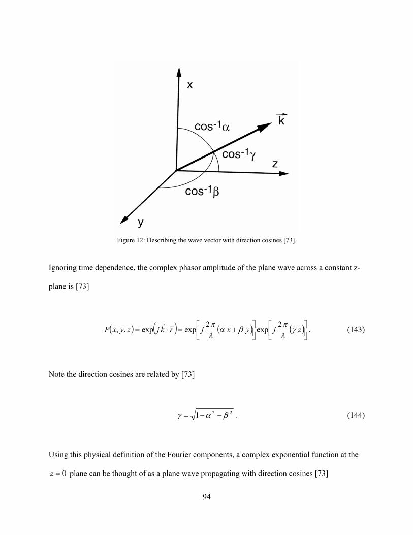
94

Figure 12: Describing the wave vector with direction cosines [73].

Ignoring time dependence, the complex phasor amplitude of the plane wave across a constant z-

plane is [73]

( ) ( ) ( ) ( )⎥⎦⎤

⎢⎣⎡

⎥⎦⎤

⎢⎣⎡ +=⋅= zjyxjrkjzyxP γ

λπβα

λπ 2exp2expexp,, rr

. (143)

Note the direction cosines are related by [73]

221 βαγ −−= . (144)

Using this physical definition of the Fourier components, a complex exponential function at the

0=z plane can be thought of as a plane wave propagating with direction cosines [73]

95

( ) ( )221 YXYX ffff λλγλβλα −−=== . (145)

In the Fourier decomposition of U with spatial frequencies ( )YX ff , the complex amplitude of

the plane wave is ( ) YXYX dfdfffA 0;, , where λα=Xf and λβ=Yf . Therefore the angular

spectrum of ( )0,, yxU is [73]

( )∫ ∫∞

∞−⎥⎦

⎤⎢⎣

⎡⎟⎠⎞

⎜⎝⎛ +−=⎟

⎠⎞

⎜⎝⎛ dydxyxjyxUA

λβ

λαπ

λβ

λα 2exp0,,0;, . (146)

5.4 2-D Fourier Transform of the Mutual Coherence Function

The MCF is defined as the second-order moment of the optical field after propagating through

turbulence. The Fourier Transform of the correlation function of the received optical field yields

the power spectral density of the field. The PSD can be interpreted as the power distribution in

the random amplitudes of the plane waves, or using the angular spectrum, the angular power.

The angular spread of a spherical wave propagating through turbulence can be calculated from

the two-dimensional Fourier transform of the MCF. Assuming a radially symmetric MCF, the

observation points are related by 21 rr −=ρ [7].

The magnitude of the MCF for a spherical wave is given by [7]

96

( ) ( )⎥⎦⎤

⎢⎣⎡−=Γ LDIL sp ,

21exp, 02 ρρ (147)

where ( )2

00

4 LP

Iπ

= is the received irradiance without turbulence effects, 0P is the transmitted

optical power and ( )24 Lπ represents the power decrease as the propagating wave spreads.

( )LDsp ,ρ is the wave structure function for a spherical wave, assuming Kolmogorov turbulence

[7],

( )⎪⎩

⎪⎨⎧

<<<<

<<=

−

003522

0231

022

09.1

09.1,

LlLkC

lLlkCLD

n

nsp ρρ

ρρρ (148)

The angular spectrum arises from the two-dimensional Fourier transform of the MCF. Due to

the radial symmetry of the MCF, the two-dimensional Fourier transform becomes the Fourier-

Bessel transform, also known as the Hankel transform of zero order. The Hankel transform of

zero order is defined by [14]

( ){ } ( ) ( ) ρρρπρπ drJfrg 22 00

0 ∫∞

=H (149)

The Hankel transform of the MCF is then defined as

97

( ){ } ( ) ( ) ( ) ρρρπρπρ drJLrSL 2,2, 00

220 ∫∞

Γ==ΓH (150)

( ) ( ) ( ) ρρρπρπ drJaIrS b 2exp2 00

0 ∫∞

−= (151)

where 35,2=b as shown in (148) and

[ ][ ]⎪⎩

⎪⎨⎧

<<<<

<<=

−

−−

003522

0231

022

55.0

55.0

LlmLkC

lmLlkCa

n

n

ρ

ρ (152)

For the regime 0l<<ρ , 2=b , see (148), the transform becomes

( ) ( ) ( ) ρρρπρπ drJaIrS 2exp2 00

20 ∫∞

−= (153)

Using the integral relation [7]

( ) 0,0,4

exp2

1

02

2

2022

>>⎟⎟⎠

⎞⎜⎜⎝

⎛−=∫

∞− ba

ab

adxbxJxe xa (154)

we have

98

( ) ( )⎟⎟⎠

⎞⎜⎜⎝

⎛−=

ar

aIrS

2

0 exp ππ . (155)

For the regime 00 Ll <<<< ρ , 35=b , see (148), the transform becomes


350 ∫∞

−= , (156)

where the integration is carried out in APPENDIX B. The spectrum in Watts is approximated by

( )

( )

( )[ ]W

Lr

la

r

aI

lr

ar

aI

rS

⎪⎪⎪

⎩

⎪⎪⎪

⎨

⎧

>>>>⎟⎟⎟

⎠

⎞

⎜⎜⎜

⎝

⎛−

>>⎟⎟⎠

⎞⎜⎜⎝

⎛−

≈

0056

2

560

0

2

0

22

9.0exp47.3

2exp

πππ

πππ

(157)

5.4.1 Relating angular spectrum and spatial spectrum

The spatial spectrum, S(r) can be expressed in terms of direction cosines. The direction cosines

are given by

99

γθ

λβθλαθ

=

====

z

yy

xx

ff

cos

coscos

. (158)

Since the direction cosines are related by

1coscoscos 222 =++ zyx θθθ , (159)

( ) ( )221cos YXz ff λλγθ −−== . (160)

It is assumed the spatial frequencies are symmetrical thus cylindrical coordinates can be used

such that

222yx ffr += . (161)

Substituting yields

221cos rz λθ −= . (162)

Using the trigonometric identity

2222 sin11cos zz r θλθ −=−= , (163)

100

222 sin zr θλ = . (164)

Performing a Taylor expansion about zθ and retaining the first term for small angles yields

λθ zr ≅ . (165)

This is the relationship between the radial parameter of the two-dimensional Fourier Transform

of the MCF and the angular spread from the z-axis.

5.5 Wavenumber PDF

Fully developed atmospheric turbulence is a cascade process of large eddies on the order of the

outer scale continually breaking into smaller eddies on the order of the inner scale and then

dissipating. This continuum of eddies occurs approximately within the volume of the large eddy.

The three-dimensional power spectrum of the eddies represents average refractive power among

the continuum of eddies and obeys a 311− power law within the inertial subrange,

( )00

3112 11033.0Ll

Cn >>>>=Φ − κκκ , (166)

101

where Rπκ 2= is interpreted as the spatial wavenumber for an eddy with size R. The power

spectrum normalized by the total refractive power i.e. the integral of the power spectrum over all

spatial wavenumbers, of the eddies can be interpreted as a PDF of the spatial wavenumbers

present within the turbulence [76]. Here we are interested in the PDF of spatial wavenumbers

lying within the inertial subrange and along a single dimension.

The three-dimensional power spectrum can be reduced to the one-dimensional power spectrum

in the case of a statistically homogeneous and isotropic field using the relation [7, 76]

( ) ( )κκ

κπκ

dVd

21

−=Φ , (167)

where ( )κV is the one-dimensional spectrum. Solving for ( )κV yields

( ) ( )∫∞

∞−

Φ−= κκκπκ dV 2 . (168)

Completing the integration gives

( )00

352 11033.05

6Ll

CV n >>>>= − κκπκ . (169)

102

To form the PDF of spatial wavenumbers lying within the inertial subrange, we first find the

total refractive power within the inertial subrange

( )⎥⎥⎦

⎤

⎢⎢⎣

⎡−=

−−

∫32

0

32

0

21

1

11033.05

90

0lL

CdV n

l

L

πκκ . (170)

The PDF is then the one-dimensional spectrum normalized by the total refractive power

( )0032

0

32

0

35 11

1132

Ll

lL

p >>>>

⎥⎥⎦

⎤

⎢⎢⎣

⎡−

=−−

−κκκ (171)

5.6 Probability Density Function of Received Irradiance

We begin with the random portion of the received spatial optical field as derived in 5.2, equation

(138)

( ) ( )∑=

=M

jjj weE

0rr , (172)

103

where M is the number of spatial modes, ( )rjw defines the spatial modes (plane waves), and je

is the random amplitude of the spatial modes. The random amplitude coefficients je are

themselves a sum

∑=

==n

1

Rek

ik

ij

kere θθ , (173)

where n is a random number representing the number of effective eddies, or scatterers, along the

propagation path. The amplitude of each spatial mode is a sum of zero mean, circular complex,

Gaussian random variables with uniform phase; this is true assuming all scattering is weak [67].

The phase delay of the propagating field, introduced by the eddies, will undergo many cycles of

2π, leading to a uniform phase distribution [67]. The random variables represent the scattered

components of the optical field after passing through a scatterer.

Due to the orthogonality of the spatial modes in the set ( )}{ rjw ,

( ) ( )∫ =A

jj dww 1rrr , (174)

the irradiance of the received field can be expressed as the integral of the magnitude squared of

the optical field within the field of view of the receiver,

104

∑=

=M

jjeI

0

2. (175)

Assuming the random number n represents a large number of scatterers along the propagation

path the central limit theorem can be used [67]. Here we take je to be approximately

statistically independent. The random sum in (173) then tends to a joint distribution of Rayleigh

distributed amplitude (R) and uniform distributed phase (θ) [67].

( ) 0,exp22

2

2≥

⎟⎟⎟

⎠

⎞

⎜⎜⎜

⎝

⎛= r

R

r

R

rrpR (176)

We first derive the conditional PDF of irradiance for a fixed number of scatterers along the

propagation path, n=n . The conditional variance of the amplitude is then [67]

jk nrnR λ== 22 (177)

and the conditional PDF of the amplitude for a single spatial mode is

( ) ∞≤≤== −j

nr

j

jj re

nr

nrP jj 02 2 λ

λn . (178)

Making the change of variable to irradiance,

105

jjjj IrrI == ,2 (179)

and forming the Jacobian

jj

j dII

dr2

1= , (180)

then substituting into the amplitude PDF

( )j

nI

j

jj I

en

InIP jj

212 λ

λ−==n (181)

we get the irradiance PDF for a single spatial mode,

( ) ∞≤≤== −j

nI

jj Ie

nnIP jj 01 λ

λn . (182)

The PDF of irradiance is an exponential distribution with mean parameter jnλ . Therefore the

variance of the received field amplitude is the mean of the received field irradiance. We now

have the PDF of the irradiance of a single spatial mode 2

je and need to derive the PDF for M

spatial modes. To do this we use the property that the convolution of M PDFs is equivalent to

106

the product of M characteristic functions [9]. The derivation is carried out in APPENDIX C and

yields

( ) ∞≤≤== ∑=

− IenA

nIPM

j

nI

j

j j 01

λ

λn , (183)

where

∏≠=

−

= M

jmm j

mjA

11

1

λλ

. (184)

We must now calculate the unconditional PDF for irradiance,

( ) ( ) ( )∫∞

==0

dnnPnIPIP n . (185)

We must first derive the PDF of n. We assume the effective scatterers are Poisson distributed

and the distance between the effective scatterers is independent and exponentially distributed

with a unique mean value kγ . We assume there are a deterministic number of scatterers N along

the propagation path. We can write the PDF for a single scatterer as

107

( ) ∞≤≤= −k

n

kk nenP kk 01 γ

γ. (186)

A derivation similar to the conditional PDF of irradiance is used to derive the PDF of scatterers

along the path. The resulting PDF is

( ) ∞≤≤= ∑=

− neB

nPN

k

n

k

k k 01

γ

γ, (187)

where

∏≠=

−

= N

kll k

lkB

11

1

γγ

. (188)

Substituting into (185), the integral becomes

( ) ∑ ∫∑=

∞−−

==

N

k

nnI

k

kM

j j

j dneen

BAIP kj

1 01

1 γλ

γλ (189)

We will use the integral representation [70]

108

( ) ( )∫∞

+− >⎟⎟⎠

⎞⎜⎜⎝

⎛−−⎟

⎠⎞

⎜⎝⎛=

0

12

04

exp22

1 xdttt

xtxxK pp

p , (190)

where ( )xK p is a modified Bessel function of the second kind of order p. For a zero-order

modified Bessel function of the second kind we can write

( ) ∫∞

− >⎟⎟⎠

⎞⎜⎜⎝

⎛−−=

0

12

0 04

exp21 xdtt

txtxK . (191)

We rewrite the integral in (189) as

∫∞

−⎟⎟⎠

⎞⎜⎜⎝

⎛−

−

0

1 exp dnnn

Inkj γλ

(192)

and make a change of variable, tn k =γ to get

∫∞

−⎟⎟⎠

⎞⎜⎜⎝

⎛−

−

0

1 exp dttt

Itkjγλ

. (193)

Equating the terms in the exponential we get

kjkj

Ixxt

Iγλγλ

24

2=→= . (194)

109

We can now write the PDF for irradiance as

( ) ∑∑==

⎟⎟

⎠

⎞

⎜⎜

⎝

⎛=

N

k kjk

kM

j j

j IKBA

IP1

01

22γλγλ

. (195)

5.7 Statistical Moments of Irradiance and Scintillation Index

As stated before, the scintillation index is vital in predicting the performance of an FSO

communication system. The first and second moment of irradiance are required to calculate the

scintillation index.

5.7.1 First moment of irradiance

The mean irradiance, also known as the first moment is calculated by

( )dIIpII ∫∞

=0

. (196)

Substituting (195) we get

110

dIIIKBA

IN

k kjk

kM

j j

j∫ ∑∑∞

==⎟⎟

⎠

⎞

⎜⎜

⎝

⎛=

0 10

122

γλγλ (197)

and pulling out the constants

dIIIKBA

Ikj

N

k k

kM

j j

j∫∑∑∞

==⎟⎟

⎠

⎞

⎜⎜

⎝

⎛=

00

1122

γλγλ. (198)

The integral can be solved using the relation [7]

( )

0,1,0

21

212

01

1

>−>≥

⎟⎠⎞

⎜⎝⎛ −+

Γ⎟⎠⎞

⎜⎝⎛ ++

Γ=∫∞

+

−

app

ppa

dxaxKx p

μ

μμμ

μμ

, (199)

where ( )xK p is a modified Bessel function of the second kind of order p and ( )xΓ is the gamma

function. Making the change of variable

dvvdIvI

dII

dvIv

22

1

2 ==

=→=, (200)

and noting the limits stay the same we can concentrate on the integral

111

dvvvvKdIIIKkjkj

∫∫∞∞

⎟⎟

⎠

⎞

⎜⎜

⎝

⎛=

⎟⎟

⎠

⎞

⎜⎜

⎝

⎛

0

20

00 222

γλγλ. (201)

Identifying kj

apγλ

μ 2,0,3 === the integral becomes

( ) ( )

( )2

22

2

22

2

4

2

kj

kj

γλ

γλ

=

⎥⎥⎥⎥⎥⎥

⎦

⎤

⎢⎢⎢⎢⎢⎢

⎣

⎡

ΓΓ

⎟⎟⎠

⎞⎜⎜⎝

⎛=

. (202)

Substituting back into (198) yields

( )

∑∑∑∑====

==N

kkk

M

jjj

kjN

k k

kM

j j

j BABA

I11

2

11 22 γλ

γλγλ

. (203)

The first moment can be further simplified. Carrying out the sum for the first four terms reveals

a pattern and the first moment can be rewritten as

∑∑==

=N

kk

M

jjI

11γλ . (204)

112

5.7.2 Second moment of irradiance

The second moment is calculated by

( )dIIpII ∫∞

=0

22 . (205)

Substituting (195) we get

dIIIKBA

IN

k kjk

kM

j j

j∫ ∑∑∞

==⎟⎟

⎠

⎞

⎜⎜

⎝

⎛=

0

2

10

1

2 22γλγλ

(206)

and pulling out the constants

dIIIKBA

Ikj

N

k k

kM

j j

j∫∑∑∞

==⎟⎟

⎠

⎞

⎜⎜

⎝

⎛=

0

20

11

2 22γλγλ

. (207)

Using the integral relation in (199) we make the change of variable

dvvdIvI

dII

dvIv

22

1

2 ==

=→=, (208)

113

and noting the limits stay the same we can concentrate on the integral

( ) dvvvvKdIIIKkjkj

∫∫∞∞

⎟⎟

⎠

⎞

⎜⎜

⎝

⎛=

⎟⎟

⎠

⎞

⎜⎜

⎝

⎛

0

220

0

20 222

γλγλ. (209)

Identifying kj

apγλ

μ 2,0,5 === the integral becomes

( ) ( )

( )3

6

4

2

33

2

22

kj

kj

γλ

γλ

=

⎥⎥⎥⎥⎥⎥

⎦

⎤

⎢⎢⎢⎢⎢⎢

⎣

⎡

ΓΓ

⎟⎟⎠

⎞⎜⎜⎝

⎛=

. (210)

Substituting back into (207)

( ) ∑∑∑∑====

==N

kkk

M

jjjkj

N

k k

kM

j j

j BABA

I1

2

1

23

11

2 422 γλγλγλ

(211)

The second moment can be further simplified. Carrying out the sum for the first four terms

reveals a pattern and the second moment can be rewritten as

114

⎥⎥

⎦

⎤

⎢⎢

⎣

⎡

⎟⎟⎠

⎞⎜⎜⎝

⎛+

⎥⎥⎥

⎦

⎤

⎢⎢⎢

⎣

⎡

⎟⎟

⎠

⎞

⎜⎜

⎝

⎛+=

⎟⎟

⎠

⎞

⎜⎜

⎝

⎛++

⎟⎟

⎠

⎞

⎜⎜

⎝

⎛++=

⎟⎟

⎠

⎞

⎜⎜

⎝

⎛+

⎟⎟

⎠

⎞

⎜⎜

⎝

⎛+=

∑∑∑∑

∑ ∑∑∑∑ ∑∑∑

∑ ∑∑∑ ∑∑

====

−

= +===

−

= +===

−

= +==

−

= +==

2

11

22

11

2

1

1 11

2

1

21

1 11

2

1

2

1

1 11

21

1 11

22

22

2222

N

kk

N

kk

M

jj

M

jj

N

ss

N

srr

N

kk

N

kk

M

ss

M

srr

M

jj

M

jj

N

ss

N

srr

N

kk

M

ss

M

srr

M

jjI

γγλλ

γγγγλλλλ

γγγλλλ

. (212)

5.7.3 Scintillation index

The scintillation is defined as the normalized second moment,

12

2

2

222 −=

−=

I

I

I

IIIσ . (213)

Substituting (204) and (212) yields

12

11

2

11

22

11

2

2 −

⎥⎥⎦

⎤

⎢⎢⎣

⎡

⎥⎥

⎦

⎤

⎢⎢

⎣

⎡

⎟⎟⎠

⎞⎜⎜⎝

⎛+

⎥⎥⎥

⎦

⎤

⎢⎢⎢

⎣

⎡

⎟⎟

⎠

⎞

⎜⎜

⎝

⎛+

=

∑∑

∑∑∑∑

==

====

N

kk

M

jj

N

kk

N

kk

M

jj

M

jj

I

γλ

γγλλ

σ . (214)

115

The scintillation index can be rewritten as follows

111

1

2

1

1

2

2

1

1

2

2

1

2

11

2

2

1

2

11

2

2

−

⎟⎟⎟⎟⎟⎟

⎠

⎞

⎜⎜⎜⎜⎜⎜

⎝

⎛

⎥⎥⎦

⎤

⎢⎢⎣

⎡+

⎟⎟⎟⎟⎟⎟⎟

⎠

⎞

⎜⎜⎜⎜⎜⎜⎜

⎝

⎛

⎥⎥⎦

⎤

⎢⎢⎣

⎡+=

−

⎥⎥⎦

⎤

⎢⎢⎣

⎡

⎥⎥

⎦

⎤

⎢⎢

⎣

⎡

⎟⎟⎠

⎞⎜⎜⎝

⎛+

⎥⎥⎦

⎤

⎢⎢⎣

⎡

⎥⎥⎥

⎦

⎤

⎢⎢⎢

⎣

⎡

⎟⎟

⎠

⎞

⎜⎜

⎝

⎛+

=

∑

∑

∑

∑

∑

∑∑

∑

∑∑

=

=

=

=

=

==

=

==

N

kk

N

kk

M

jj

M

jj

N

kk

N

kk

N

kk

M

jj

M

jj

M

jj

I

γ

γ

λ

λ

γ

γγ

λ

λλ

σ

. (215)

Carrying the multiplication of the two terms

12 2

1

1

2

2

1

1

2

2

1

1

2

2

1

1

2

2 −

⎟⎟⎟⎟⎟⎟

⎠

⎞

⎜⎜⎜⎜⎜⎜

⎝

⎛

⎥⎥⎦

⎤

⎢⎢⎣

⎡

⎟⎟⎟⎟⎟⎟⎟

⎠

⎞

⎜⎜⎜⎜⎜⎜⎜

⎝

⎛

⎥⎥⎦

⎤

⎢⎢⎣

⎡+

⎥⎥⎦

⎤

⎢⎢⎣

⎡+

⎥⎥⎦

⎤

⎢⎢⎣

⎡=

∑

∑

∑

∑

∑

∑

∑

∑

=

=

=

=

=

=

=

=

N

kk

N

kk

M

jj

M

jj

N

kk

N

kk

M

jj

M

jj

I

γ

γ

λ

λ

γ

γ

λ

λ

σ . (216)

Since jλ and kγ are positive terms then the following inequality is valid for a single term in each

of the summations

∑∑∑∑====

≥⎥⎥⎦

⎤

⎢⎢⎣

⎡≥

⎥⎥⎦

⎤

⎢⎢⎣

⎡ N

kk

N

kk

M

jj

M

jj and

1

22

11

22

1γγλλ . (217)

116

Therefore, the theoretical maximum allowable scintillation index is 32 =Iσ

5.8 Relating Model Parameters to Physical Quantities

In this section, the model parameters of the PDF, namely the s'λ and s'γ , are related to physical

measurable quantities of the optical wave. The solution of (65) would have yielded the exact

eigenfunctions and eigenvalues for the spatial modes. However, we chose to simplify the

problem via an engineering approximation which leads to spatial eigenfunctions of the form of

two-dimensional plane waves. Saleh [75] points out that when the eigenfunctions of the KL

expansion are approximated with harmonic eigenfunctions (sinusoids), the eigenvalues are then

approximated by samples from the Fourier Transform of the correlation function. Recall the

definition of the angular spectrum derived in section 5.3. The physical behavior of the received

irradiance can be analyzed in two planes, aperture and focal. The two planes are related through

the Fourier transform and have a reciprocal relationship. The physical interpretation of the

model parameters are described in both the aperture plane and focal plane for completeness.

117

5.8.1 Sampling the spatial spectrum

Recall an approximation to the KL expansion was performed on the received optical field. The

spatial spectrum of the optical wave was derived by taking the two-dimensional Fourier

Transform of the MCF. Assuming the received optical field is stationary, then in the limit of the

radial distance ρ much larger than the width of the mutual coherence function ( )ρsΓ at the 1/e

point, we have [75]

( ) MjjrrScut

jjj ,,2,1,2, K==≅ρπλ (218)

where j is an integer, cutρ is the radial distance much larger than the 1/e point of the MCF, each

jλ is the corresponding eigenvalue of the eigenfunctions defined by the approximation to the KL

expansion, and ( )jrS is a sample of two-dimensional Fourier Transform of the MCF. This

assumption can be made if the sampling is so fine such that rΔ is infinitesimally small, however

the units are not consistent. As stated in section 5.6, the variance of the received field amplitude

is the mean of the received field irradiance. This implies each eigenvalue, λ should have units

of irradiance [W/m2], while sampling S(r) yields units of [W]. This discrepancy is noted,

however due to the nature of the approximations being made it is dismissed and the units are

taken to be that of irradiance.

118

There is no formal definition of how much larger ρ should be compared to the 1/e point of the

MCF. After experimenting with many values a value of 250 times the 1/e point of the MCF was

chosen, this allowed the model to avoid numerical issues over a broad range of conditions. The

numerical issues encountered are discussed in APPENDIX E in more detail.

From (157), the spatial spectrum is only valid within the inertial subrange defined by the inner

and outer scales of turbulence. Upper and lower cutoff values were chosen as 0

221

lmπκ = and

00

22Lπκ = respectively. Again, experimenting with several other cutoff values, the values

chosen allowed the model to avoid numerical issues over a broad range of conditions.

The total number M of s'λ is related to aperture size. As the aperture size increases, M

increases, this accounts for aperture averaging. Increasing M is physically equivalent to more

spatial plane waves being collected in the aperture plane. On the other hand, increasing M is also

physically equivalent to less angular modes being collected in the focal plane, i.e. the field of

view is reduced with a larger aperture. Parseval’s theorem requires the integral of the spatial

spectrum yield the total irradiance, 0I ; i.e. energy conservation. Since the spatial spectrum is

only sampled within the upper and lower cutoffs, the sum of the lambdas will never equal 0I .

However, as defined in (204) the first moment, or mean irradiance, is the product of the sum of

the lambdas and gammas. The PDF of irradiance is typically plotted with data normalized by the

mean irradiance. In log space, this roughly centers the PDF about 0 dB. In order to normalize

the theoretical PDF to a mean irradiance of unity, the following constraint is defined

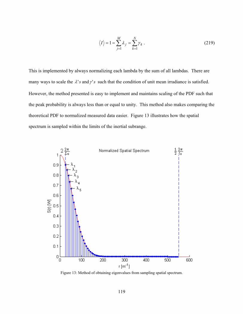
119

∑∑==

===N

kk

M

jjI

111 γλ . (219)

This is implemented by always normalizing each lambda by the sum of all lambdas. There are

many ways to scale the s'λ and s'γ such that the condition of unit mean irradiance is satisfied.

However, the method presented is easy to implement and maintains scaling of the PDF such that

the peak probability is always less than or equal to unity. This method also makes comparing the

theoretical PDF to normalized measured data easier. Figure 13 illustrates how the spatial

spectrum is sampled within the limits of the inertial subrange.

Figure 13: Method of obtaining eigenvalues from sampling spatial spectrum.

120

5.8.2 Sampling the wavenumber PDF

We are interested in the distribution of the number of effective scatterers along the propagation

path. In section 5.5 a PDF was derived based upon the one-dimensional refractive index power

spectrum of the atmosphere. Physically this represents the probability density of encountering

eddies with a particular spatial wavenumber within the turbulence.

We assume the propagating wave encounters a finite deterministic number of scatterers along the

path. The irradiance of each spatial mode is a product of the number of scattered components N

contributing to the irradiance. The number of scattered components captured by an aperture is

defined by N. For a point aperture 1=N , i.e. one scattered component of the wave is detected.

As the aperture size increases, it captures more scattered components of the received optical field

in the aperture plane and N increases. On the other hand, increasing N is equivalent to receiving

less angular components in the focal plane, i.e. the field of view is reduced with a larger aperture.

The s'γ will be calculated by integrating a portion of the wavenumber PDF, such that each

γ represents a probability and is unitless.

From (171), the wavenumber PDF is only valid within the inertial subrange defined by the inner

and outer scales of turbulence. The wavenumber PDF can be generalized to any upper and lower

cutoff values,

( ) [ ] 1232320

35

32 κκκ

κκκκ >>>>−

=−−

−

mp (220)

121

where mκ and 0κ are the upper and lower cutoffs respectively. Upper and lower cutoff values

were chosen as 0

221

lmπκ = and

00

22Lπκ = respectively. The s'γ are then calculated by

dividing the valid region of the wavenumber PDF into N equally spaced segments,

( ) ( ) ( )∫∫∫=m

kN

N

N

N

j dpdpdpκ

κ

κκκκκκγγγ ,,,,,,2

1

1

0

21 KK . (221)

Figure 14 shows an illustration of calculating the s'γ by integrating the wavenumber PDF, this

graph corresponds to 20=N .

Figure 14: Method of calculating gammas from integrating the wavenumber PDF; N=20.

122

6 EXPERIMENTATION

Irradiance data were collected over a 1km horizontal path for several different sized receiving

apertures. The data were collected under moderate-to-strong turbulence conditions. The path

was instrumented with scintillometers and anemometers to provide real time atmospheric data.

Histograms were formed with the data and compared to the existing Gamma-Gamma PDF

model, as well as the new PDF developed.

6.1 Overview

The experiment was performed at the Innovative Science and Technology Experimental Facility

(ISTEF) laser range in Cape Canaveral, Kennedy Space Center, Florida. The range is 1km long

and approximately 14m wide. There was 1-2m high vegetation surrounding the length of the

range. The propagation path was trimmed grass kept at approximately 5cm tall. A mobile laser

propagation laboratory was placed at the north end of the range to provide a clean and dry

environment to operate equipment. The mobile laboratory was equipped with an isolated 122cm

x 244cm optical bench supported from the ground separate from the mobile lab, 5kVA

uninterruptible power supply, safety glasses, laser curtain, air conditioner, and a removable

window to propagate through. The ISTEF laser lab was located at the north end of the range and

provided an air conditioned environment for the transmitting equipment. Figure 15 illustrates the

layout of the experimental setup on the ISTEF laser range.

123

The transmitter system consisted of a CW 532nm DPSS laser and optics to diverge the beam

such that it was approximately a spherical wave at the receiver. The receiver system consisted of

a 154mm (6”) refracting telescope outfitted with several removable apertures. The telescope was

coupled with a high-speed, high-dynamic range power meter. The output of the power meter

was sampled using a digitizer controlled with LabVIEW SignalExpress. In addition to the

experimental setup, a suite of equipment was setup to characterize the atmosphere along the

optical propagation path. Three scintillometers were used to measure the Cn2 along the path, two

of which were also capable of measuring the inner scale. Three sonic anemometers were

positioned along the path to measure the three-dimensional wind vector.

124

Figure 15: Layout of equipment on 1km laser range. Three scintillometers were used to provide path-averaged Cn

2 and l0. Three 3-axis anemometers provided the crosswind at points along the path.

Parallel to the experimental propagation path were three commercial scintillometers, one model

Scintec BLS900 and two model Scintec SLS-20. The BLS900 scintillometer provided a path-

averaged value of Cn2 and an estimate of the path-averaged crosswind speed over the 1km

propagation path. The SLS 20 scintillometers provided a path-averaged value of Cn2 and a path-

average value of the inner scale of turbulence, l0 for a 100m path. The scintillometers were

positioned on the laser range to verify the assumption of homogenous turbulence along the path.

In addition to the scintillometers, three 3-axis sonic anemometers were positioned along the path.

125

The reported crosswind from the anemometers was used to verify homogeneity as well as verify

the assumption of frozen turbulence.

6.2 Equipment

This section goes into detail about the key system elements of the experimentation;

scintillometers, transmitter, and receiver. Design details as well as theory of operation are

discussed.

6.2.1 Scintillometer – path averaged Cn2

The Scintec BLS 900 is a commercially available scintillometer capable of calculating Cn2 and

cross wind speed directly from optical measurements. The instrument boasts an operable range

of 0.5km-5km as well as valid measurements in all regimes of turbulence. The BLS series of

scintillometers is based upon the assumption of weak turbulence and utilizes aperture averaging

theory developed in the late 1970’s [77]. The scintillometer hardware consists of two incoherent

transmitting disks and one receiving aperture, all approximately the same diameter. Proper

selection of transmit and receive apertures allow the scintillometer to provide accurate Cn2

measurements without taking into account the inner and outer scale effects.

126

Under weak irradiance fluctuations, the scintillation index and the log-amplitude variance are

directly proportional to Cn2. Weak fluctuations become strong fluctuations by increasing Cn

2 or

the propagation distance, or both, for a fixed wavelength. Under strong irradiance fluctuations

(saturation) the linear relation between the log-amplitude variance and Cn2 no longer holds. The

BLS 900 is claimed to be relatively insensitive to strong fluctuation effects due to its large

incoherent emission and reception apertures. Therefore, its operation is described by the use of

weak scattering theory.

The BLS 900 has two transmitters and one receiver. The two transmitting disks consist of nearly

1000 infrared LEDs and are 15cm in diameter. Each transmitter disk has a different modulation

frequencies, this reduces the background and allows the two signals to be separated by a single

detector in the receiver. The receiver consists of a 14.5cm lens which collimates the incoming

radiation onto two silicon photodiodes. One photodiode is used to sense the turbulence-induced

fluctuations, while the other is strictly for alignment. The fluctuations received by the

photodiode are processed with a signal-processing unit made by Scintec, the calculation results

are then sent to a PC running Scintec’s BLSRun software[78].

The scintillometer measures the average received intensity from disk 1 and 2, <I1> and <I2>,

respectively, as well as their variances, σ11 and σ22, and covariance, σ12. These statistical

quantities can be related to the log-amplitude variances B11, B22, and covariance B12 under the

assumption of log-normal statistics by the relations [78]

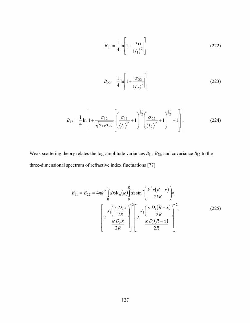
127

⎥⎥⎦

⎤

⎢⎢⎣

⎡+= 2

1

1111 1ln

41

IB

σ (222)

⎥⎥⎦

⎤

⎢⎢⎣

⎡+= 2

2

2222 1ln

41

IB σ (223)

⎥⎥⎥

⎦

⎤

⎢⎢⎢

⎣

⎡

⎥⎥⎥

⎦

⎤

⎢⎢⎢

⎣

⎡

−⎟⎟

⎠

⎞

⎜⎜

⎝

⎛+⎟

⎟

⎠

⎞

⎜⎜

⎝

⎛++= 1111ln

41

21

22

222

1

21

11

2211

1212

IIB

σσσσ

σ . (224)

Weak scattering theory relates the log-amplitude variances B11, B22, and covariance B12 to the

three-dimensional spectrum of refractive index fluctuations [77]

( ) ( )

( )

( )

2

1

2

1

0 0

222

2211

2

22

2

22

2sin4

⎥⎥⎥⎥

⎦

⎤

⎢⎢⎢⎢

⎣

⎡

−

⎟⎠⎞

⎜⎝⎛ −

⎥⎥⎥⎥

⎦

⎤

⎢⎢⎢⎢

⎣

⎡⎟⎠⎞

⎜⎝⎛

×⎟⎟⎠

⎞⎜⎜⎝

⎛ −Φ== ∫ ∫

∞

RxRD

RxRD

J

RxD

RxDJ

kRxRxkdxdkBB

t

t

r

r

R

n

κ

κ

κ

κ

κκπ

, (225)

128

( ) ( )

( )

( )

2

1

2

1

00 0

222

12

2

22

2

22

12

sin4

⎥⎥⎥⎥

⎦

⎤

⎢⎢⎢⎢

⎣

⎡

−

⎟⎠⎞

⎜⎝⎛ −

⎥⎥⎥⎥

⎦

⎤

⎢⎢⎢⎢

⎣

⎡⎟⎠⎞

⎜⎝⎛

×⎟⎟⎠

⎞⎜⎜⎝

⎛⎟⎠⎞

⎜⎝⎛ −⎟

⎟⎠

⎞⎜⎜⎝

⎛ −Φ= ∫ ∫

∞

RxRD

RxRD

J

RxD

RxDJ

RxSJ

kRxRxkdxdkB

t

t

r

r

t

R

n

κ

κ

κ

κ

κκκπ

, (226)

where λπ2=k is the wavenumber, x is the length coordinate along the propagation path, R is

the propagation path length, Dr, and Dt are the receiver and transmitter diameters, respectively.

The two J1 Bessel function terms account for finite circular incoherent transmitting and receiving

apertures.

The three-dimensional spectrum used by the scintillometer is given by [78]

( ) ( ) ( )003/112033.0 LFfCnn κκλκκ −=Φ (227)

where ( )0κλf and ( )0LF κ represent the effects of l0 and L0, respectively. The inner scale effects

approach unity as 0/1 l<<κ and the outer scale effects approach unity as 0/1 L>>κ . Since the

inner scale is typically on the order of millimeters and the outer scale is typically on the order of

meters, the diameters chosen for the size of the radiating disks are not affected by the inner or

outer scale. Also, by having the disks much larger than the Fresnel zone Rλ , the wavelength

dependence is also eliminated. These assumptions are used to create a scintillometer

independent of inner, outer scale, and wavelength.

129

Inserting (227) into (225), the integration leads to the following approximate expression [77]

33722

33711

2 −− == RDBRDBC trtrn αα , (228)

where the scaling factor 629.4=rα for the BLS 900 and is dependent upon the ratio of the

transmitting and receiving apertures [78].

For the case of strong turbulence the above equations are modified with the addition of a short-

term modulation transfer function (MTF) [79]. The BLS accounts for the saturation effects in

strong turbulence by using a look-up table to scale the log-amplitude variance defined in (225)

[78].

In weak turbulence, absorption fluctuations caused by a reduction in transmission along the path,

such as fog and dust, are taken into account by the scintillometer. If not accounted for, the

absorption fluctuations could be falsely interpreted as scintillation effects from the turbulence.

From the calculated Cn2 the BLS 900 computes a slew of other atmospheric parameters such as

Fried’s parameter, scintillation at a point detector for spherical and plane waves, and the

structure function of phase. The BLS 900 also computes the cross wind speed from the time-

lagged cross-covariance function [78].

130

6.2.2 Scintillometer – path averaged Cn2 and l0

The Scintec SLS 20 is a commercially available scintillometer capable of calculating Cn2 and l0

directly from optical measurements. The instrument is restricted to weak fluctuation conditions

and therefore operates over a maximum range of 150m. The scintillometer hardware consists of

two coherent emitters, separated by a fixed distance perpendicular to the propagation path. The

receiver has two detectors separated by the same distance as the transmitters to observe the

radiation. The detectors are aligned to produce two parallel paths between the transmitter and

receiver [80].

Under weak irradiance fluctuations, the scintillation index and the log-amplitude variance are

directly proportional to Cn2. Therefore equations (222) through (225) are valid for this

scintillometer. The covariance of the logarithm of the amplitude of the received radiation (226)

is simplified for this scintillometer on account of the two parallel paths with equal diameter

transmit and receive elements [80]

( ) ( ) ( )

2

1

00 0

222

12

2

222

sin4

⎥⎥⎥⎥

⎦

⎤

⎢⎢⎢⎢

⎣

⎡⎟⎠⎞

⎜⎝⎛

⎟⎟⎠

⎞⎜⎜⎝

⎛ −Φ= ∫ ∫

∞

RxDR

xDJdJ

kRxRxkdxdkB

R

n κ

κ

κκκπ , (229)

where λπ2=k is the wavenumber, x is the length coordinate along the propagation path, R is

the propagation path length, D is the receiver and transmitter diameters, and d is the separation

131

distance of the transmitters and receivers. This formula is referenced from the operations manual

of the instrument, but the covariance equation mixes plane wave and spherical wave theory

without any justification; see pg. 280 of [7] for proper equations. The operation manual states

the transmitter uses spatial filter pinholes; therefore it is speculated that spherical wave theory is

more appropriate than plane wave theory. The log-amplitude variances B11, B22 are derived from

(229) by letting 0=d .

The three-dimensional spectrum used by the scintillometer is given by [80]

( ) ( )03/112033.0 λκκκ fCnn

−=Φ (230)

where ( )0κλf takes the form of Hill’s model and represent the effects of l0.

Both the log-amplitude variances B11, B22, and the covariance B12 are dependent upon both Cn2

and l0. However the correlation coefficient is dependent upon only l0

2

12

1

12

21

12BB

BB

BBB

r === . (231)

Therefore the instrument first calculates l0 from the correlation coefficient then references a

look-up table to calculate the inner scale effects on Cn2. From the calculated Cn

2 and l0 the SLS

20 computes a slew of other atmospheric turbulence parameters such as the structure constant for

132

temperature, the dissipation rate of the kinetic energy of turbulence, turbulent kinematic heat

fluxes and momentum, turbulent heat flux, and turbulent momentum flux [80].

6.2.3 Transmitter system

The 532nm DPSS laser had a maximum output power of approximately 800mW. As the output

power approached the maximum, the spatial mode structure transformed from the fundamental

mode to TEM20. A spatial filter on the order of 1mm was positioned in the center of the

fundamental mode to remove the additional spatial modes. Following the spatial filter was a

defocused beam expander. By inputting collimated light from the laser and defocusing the beam

expander, a good approximation to a spherical wave was achieved at the receiver. The estimated

spot diameter at the receiver was approximately 4m, including turbulence effects, indicating a

full-angle divergence of approximately 4mrad. Calculating the refractive beam parameter using

the equation [7]

20

02

kWz

=Λ (232)

yields 75, implying the receiver was very much in the far-field and thus the wavefront was

approximately spherical at the receiver. Figure 16 illustrates the optical setup at the transmitter.

133

Figure 16: Optical layout of transmitter system.

6.2.4 Receiver system

The receiving telescope and corresponding optics were recycled from a previous experiment.

The telescope was setup as a pupil plane imager. The primary lens was a single 6” diameter

refracting lens. A relay lens was placed at the focus of the primary lens such that it imaged the

pupil plane of the system. The relay lens was chosen such that a 2mm image of the pupil plane

was created at focus. The relay lens acts as a field stop for the telescope, defining the field of

view of the optical system. The advantage of this system is its minimal dependence on the focus

of the receiving telescope. To the first order, the telescope can change focus and there will

minimal effect on the light received by the detector. This is advantageous when tracking objects

at varying range, also when using Cassegrain type telescopes in an outdoor environment where

thermal variations of the telescope tube cause a shift in focus. Figure 17 illustrates the optical

components of the receiving telescope.

134

A New Focus 2101 power meter was purchased for this experiment. It has a high dynamic

range, ~70dB, and a 5mm diameter silicon photodiode. Due to the large active area of the power

meter, alignment in the focal plane of the relay lens was very forgiving. The output voltage of

the power meter was recorded with a National Instruments NI-9234 digitizer. The digitizer has

24 bits of resolution and was operated at 51.25kS/s. The digitizer was coupled with a National

Instruments NI ENET 9163 Ethernet carrier. The acquired data was controlled via LabVIEW

SignalExpress over Ethernet.

Figure 17: Optical layout of receiver system.

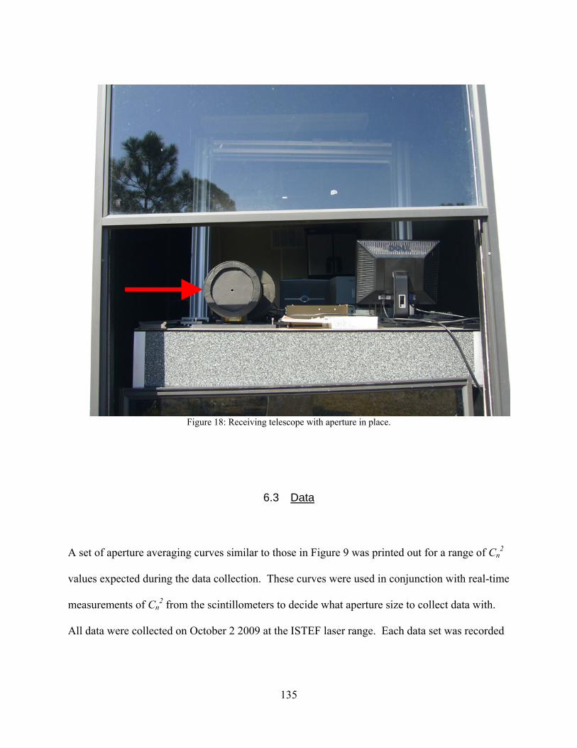
135

Figure 18: Receiving telescope with aperture in place.

6.3 Data

A set of aperture averaging curves similar to those in Figure 9 was printed out for a range of Cn2

values expected during the data collection. These curves were used in conjunction with real-time

measurements of Cn2 from the scintillometers to decide what aperture size to collect data with.

All data were collected on October 2 2009 at the ISTEF laser range. Each data set was recorded

136

over a two minute collection period. The background was measured for twenty seconds before

the start of each data set

Data were collected with a wide range of apertures such that different degrees of aperture

averaging occurred. Due to the limiting scintillation index of 3 for the new PDF, not all data is

presented, only those data sets where the calculated scintillation index was less than 3.

Each data set was processed by first converting the output of the power meter from volts to a

measured optical power as outlined in APPENDIX D. The average background was then

subtracted from each data point. The histogram of the background subtracted data set was then

created using unequal bin widths as described in section 2.1.2.1. Unequal bin widths were

necessary due to the large dynamic range of the recorded irradiance signal.

Table 1 presents the average atmospheric conditions observed over each two-minute data

collection. The crosswind speed changes on a much slower time scale than the turbulence

parameters. Throughout the three hours of data collection, the average wind speed did not

change much. At the transmitter the average wind speed was approximately 0.05 m/s, with gusts

up to 1.5 m/s in magnitude. At the middle of the path the average wind speed was approximately

0.1 m/s, with gusts up to 1.5 m/s in magnitude. At the receiver the average wind speed was

approximately 0.02 m/s, with gusts up to 2 m/s in magnitude.

The detail of the PDF is best seen on a log-log scale. The abscissa is the irradiance value

normalized by the mean irradiance ( )IILog and the ordinate is the logarithm of the

137

probability density. To the first order, in the log-log domain the PDF has the shape of an upside

down parabola or horseshoe. Physically this makes sense; the tips of the parabola represent

extremely low probability events. These events correspond to the extreme irradiance values,

deep fades and peak surges, which are known to be rare events. In each of the PDF plots below,

three curves are plotted against points from the histogram. The new PDF is fit to the data with a

best fit. The criteria of best fit are two-fold: how close did the theoretical curve match the

histogram and how close was the theoretical scintillation index to that calculated from the data.

The GG is also fit to the histogram, but a fitting algorithm was used. For comparison, the GG is

plotted with the parameters calculated according to scintillation theory. The best fit GG model is

presented to show if the model is even capable of achieving the shape of the measured PDF. The

theoretical GG model is presented to show how well scintillation theory predicts the parameters

α and β .

All of the plots were created with the corresponding atmospheric conditions presented in Table

1. The path length was fixed at 980m and the height above ground of the receiver was 2m. As

discussed in section 3.4, a constant outer scale value of mmL 8.024.00 =×= was used for all

the data sets. The outer scale is a statistical quantity and was not directly measured during the

data collection. Small variations in the outer scale undoubtedly took place as Cn2 and l0 changed

over the three hours of data collection.

138

Table 1: Atmospheric conditions observed during data collection.

Time (EST)

Aperture Diameter Size (mm)

Average Cn

2 (m-2/3) Average l0

(mm)

16:01 1.5 5.00 x 10-14 5.69 15:32 4.0 8.50 x 10-14 6.00 16:19 4.0 9.00 x 10-14 6.02 16:15 7.0 7.50 x 10-14 5.93 13:15 10.0 3.56 x 10-13 4.98 15:26 10.0 5.50 x 10-14 4.91 16:11 10.0 7.27 x 10-14 5.98 13:11 20.6 3.70 x 10-13 4.86 15:21 20.6 8.89 x 10-14 5.54 15:56 20.6 7.00 x 10-14 5.90 13:07 55.0 2.65 x 10-13 5.43 15:17 55.0 1.30 x 10-13 5.71 15:51 55.0 1.05 x 10-13 6.23 15:47 101.6 1.40 x 10-13 5.74 13:04 154.0 3.47 x 10-13 5.46 15:13 154.0 2.36 x 10-13 5.42 15:44 154.0 1.65 x 10-13 6.17 16:06 154.0 6.50 x 10-14 6.25

The following figures compare the new PDF developed in this dissertation and the GG PDF

against the histogram of the experimental data. The title identifies the time of day the data set

was recorded, the aperture size on the receiving telescope, and the Rytov variance 20β for a

spherical wave (as an indication to the strength of turbulence). The caption restates the aperture

size as well as the Cn2 from Table 1, the spatial coherence radius spρ is also presented. Printed

on each plot are the parameters used to create the PDF curves. The parameters M and N of the

new PDF were selected by eye for best fit to the histogram data, as well as closest match to the

scintillation index calculated from the data. The parameters fitα and fitβ of the best-fit GG

PDF were selected using a Levenberg-Marquardt least-squares fitting algorithm implemented by

the lsqcurvefit function in Matlab. The GG PDF was fit to the histogram data using fitα and

139

fitβ as the free-parameters. The parameters thryα and thryβ of the theoretical GG PDF were

calculated using (80) and the equations for the scintillation index of a spherical wave under

general irradiance conditions as outlined in APPENDIX A. In some of the plots, the new PDF is

truncated at low irradiance values. This is due to numerical inaccuracies of the new model; these

numerical issues are discussed in more detail in APPENDIX E.

Figure 19: New PDF, GG PDF, and histogram of data; 1.5mm aperture, Cn

2 = 5.00 x10-14, ρsp= 7.16mm.

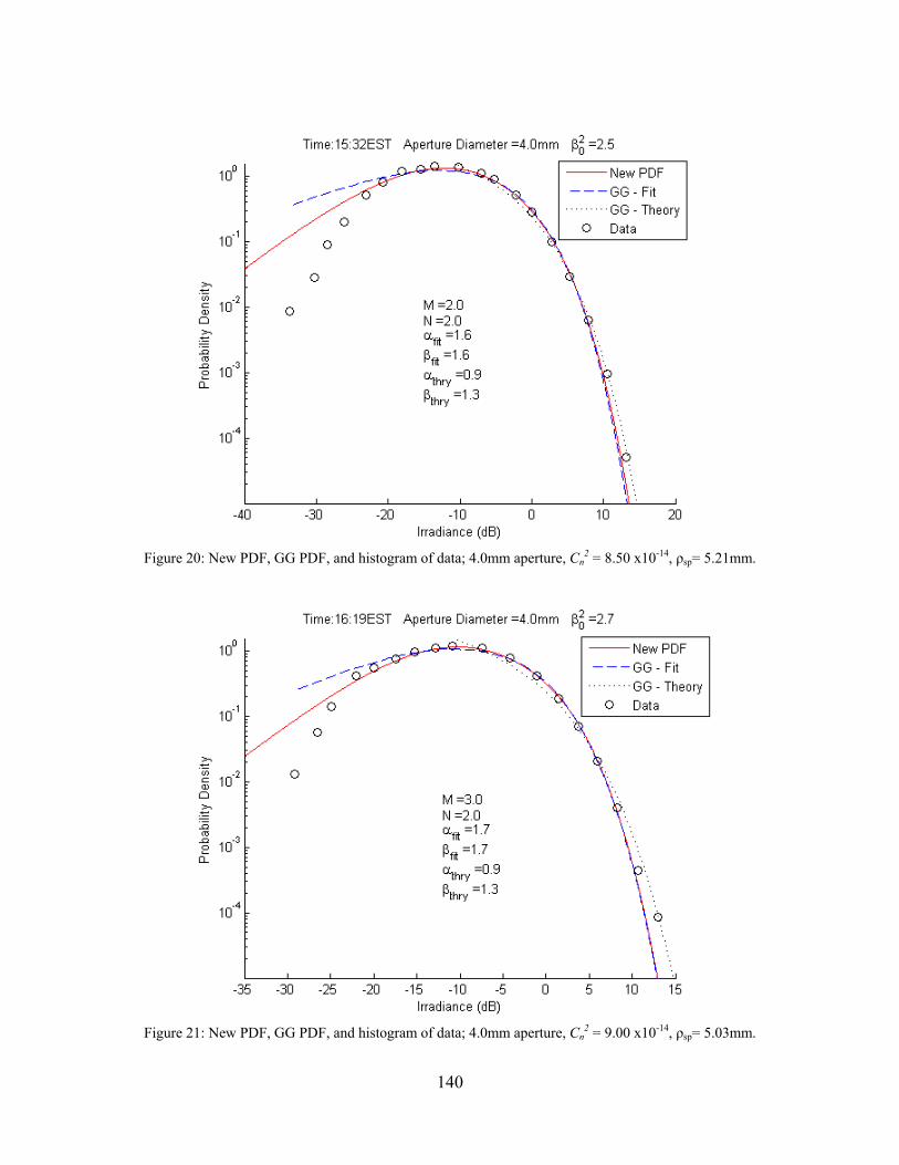
140


2 = 8.50 x10-14, ρsp= 5.21mm.


2 = 9.00 x10-14, ρsp= 5.03mm.

141


2 = 7.50 x10-14, ρsp= 5.61mm.


2 = 3.56 x10-13, ρsp= 2.21mm.

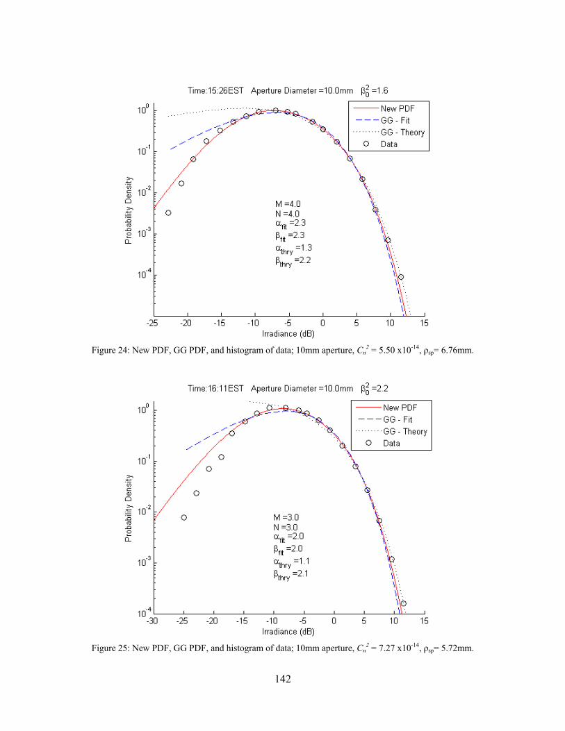
142

Figure 24: New PDF, GG PDF, and histogram of data; 10mm aperture, Cn

2 = 5.50 x10-14, ρsp= 6.76mm.

Figure 25: New PDF, GG PDF, and histogram of data; 10mm aperture, Cn

2 = 7.27 x10-14, ρsp= 5.72mm.

143


2 = 3.70 x10-13, ρsp= 2.15mm.


2 = 8.89 x10-14, ρsp= 5.07mm.

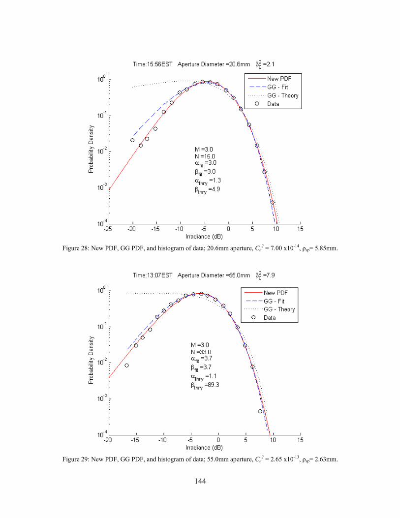
144


2 = 7.00 x10-14, ρsp= 5.85mm.


2 = 2.65 x10-13, ρsp= 2.63mm.

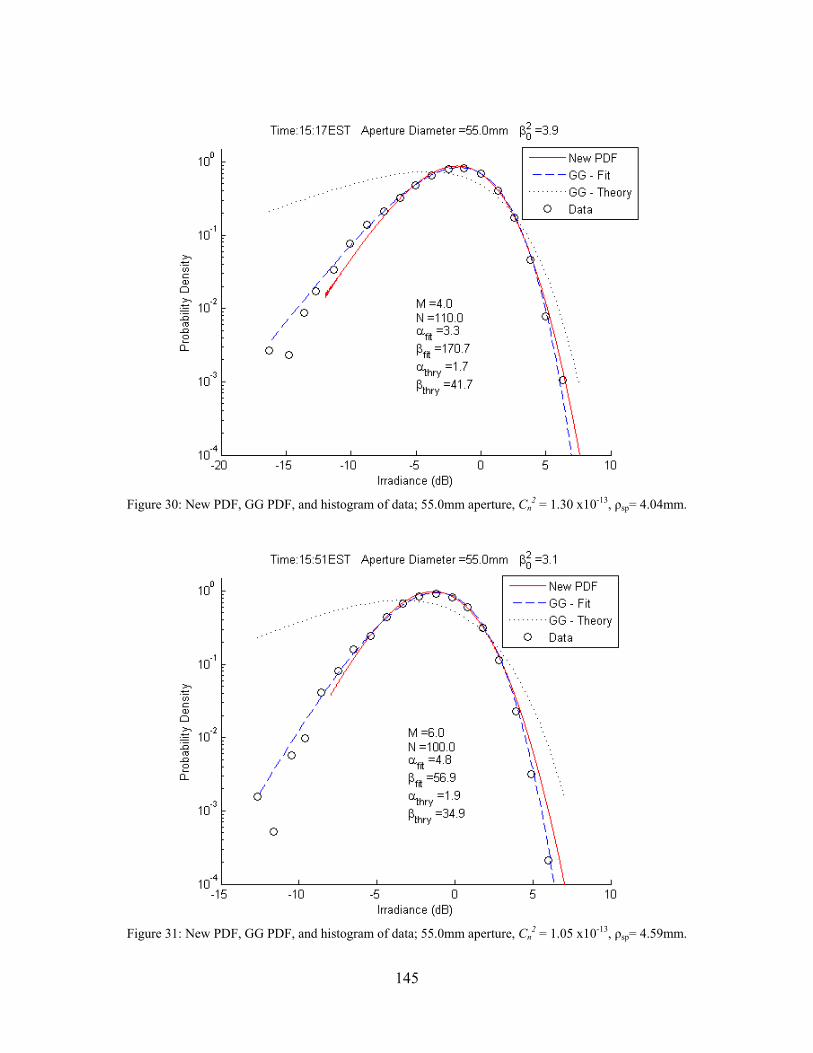
145


2 = 1.30 x10-13, ρsp= 4.04mm.


2 = 1.05 x10-13, ρsp= 4.59mm.

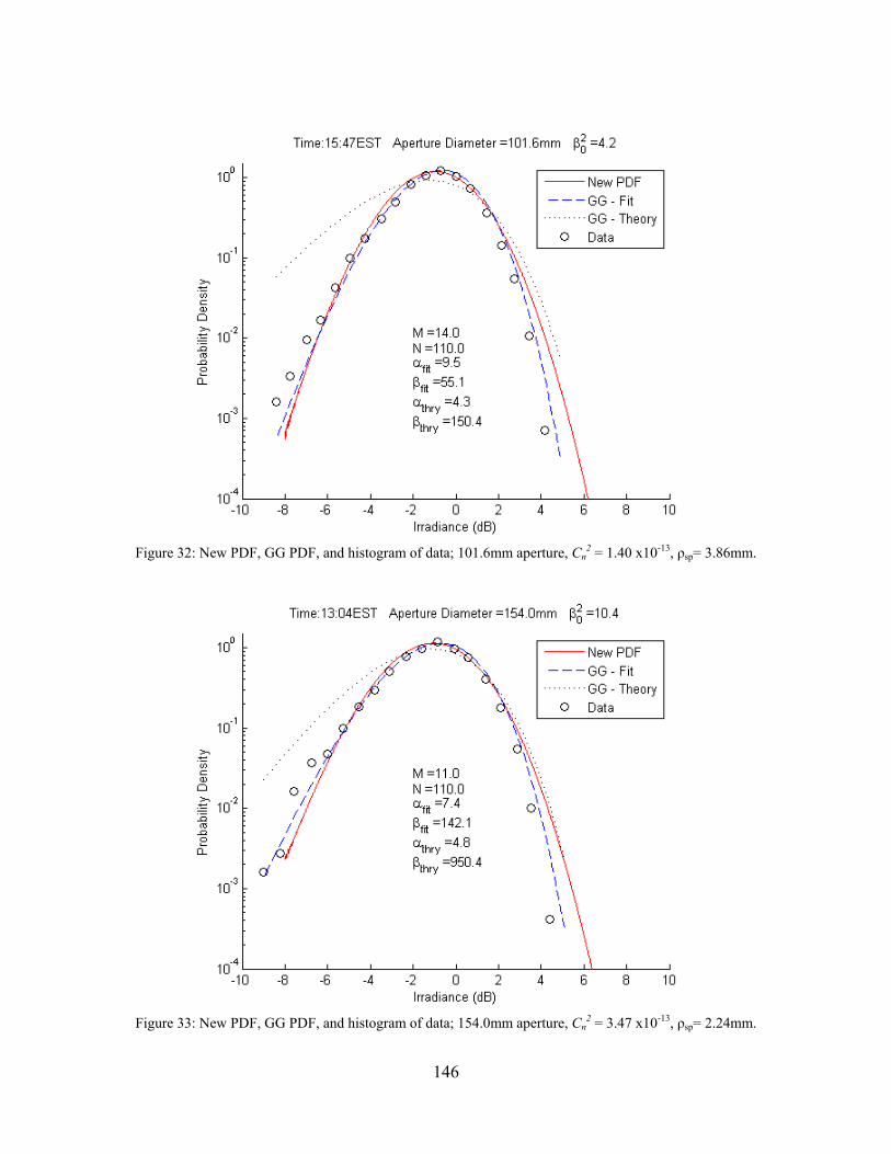
146


2 = 1.40 x10-13, ρsp= 3.86mm.


2 = 3.47 x10-13, ρsp= 2.24mm.

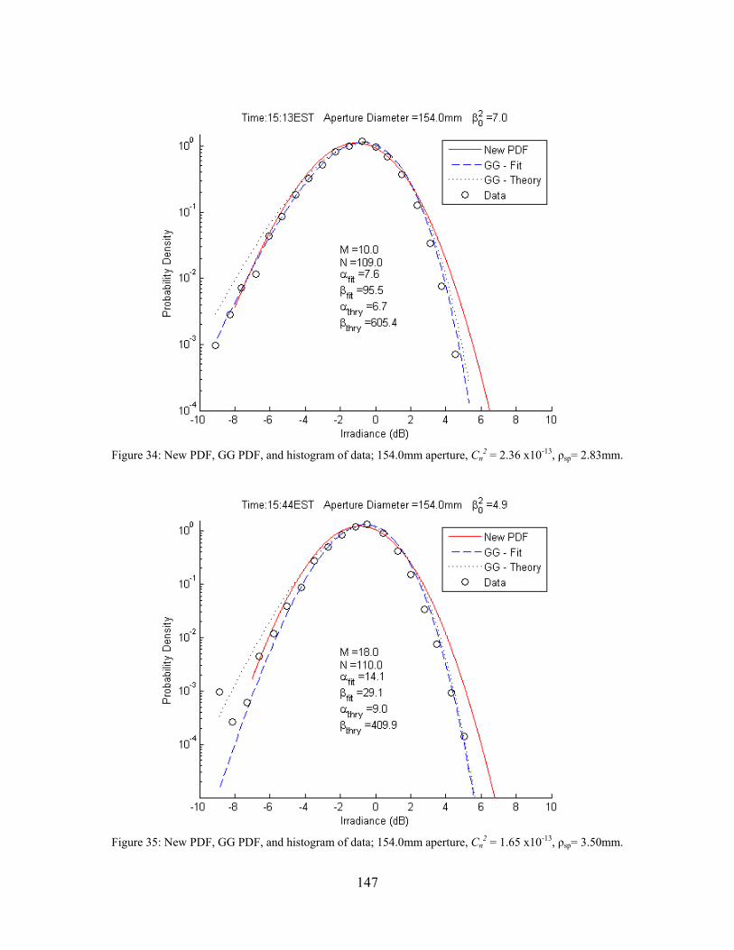
147


2 = 2.36 x10-13, ρsp= 2.83mm.


2 = 1.65 x10-13, ρsp= 3.50mm.

148


2 = 6.50 x10-14, ρsp= 6.12mm.

Table 2 compares the scintillation index values of the new PDF, GG, and experimental data. The

scintillation index of the data is calculated from the background removed experimental data

according to (71), scintillation index of the new PDF is calculated theoretically according to

(216), and the scintillation index of the GG model is calculated from (132) using the best fit

parameters.

149

Table 2: Scintillation index as calculated from the new PDF, GG fit parameters, and experimental data.

Time (EST)

Aperture Diameter

Size (mm)

SI from Data

Theoretical SI from

New PDF

SI from GG Fit

Parameters

SI from GG

Theory Parameters

16:01 1.5 1.28 1.34 1.09 1.79 15:32 4.0 2.25 1.83 1.68 2.74 16:19 4.0 1.93 1.52 1.48 2.74 16:15 7.0 1.82 1.41 1.39 2.18 13:15 10.0 2.40 1.85 1.45 2.19 15:26 10.0 1.30 1.21 1.09 1.57 16:11 10.0 1.62 1.41 1.25 1.82 13:11 20.6 1.50 1.35 1.18 1.80 15:21 20.6 1.05 1.14 0.97 1.28 15:56 20.6 0.84 0.85 0.78 1.13 13:07 55.0 0.57 0.63 0.62 0.93 15:17 55.0 0.32 0.34 0.31 0.63 15:51 55.0 0.22 0.25 0.23 0.57 15:47 101.6 0.12 0.16 0.13 0.24 13:04 154.0 0.14 0.18 0.14 0.21 15:13 154.0 0.14 0.19 0.14 0.15 15:44 154.0 0.10 0.15 0.11 0.11 16:06 154.0 0.05 0.15 0.06 0.05

Table 3 compares the parameters of the PDF models used to represent the experimental data.

150

Table 3: Parameters for new PDF and GG model used to represent experimental data.

Time (EST)

Aperture Diameter

Size (mm)

New PDF GG Fit GG Theory

M N αfit βfit αthry βthry 16:01 1.5 2.0 8.0 2.2 2.2 1.4 1.6 15:32 4.0 2.0 2.0 1.6 1.6 0.9 1.3 16:19 4.0 3.0 2.0 1.7 1.7 0.9 1.3 16:15 7.0 3.0 3.0 1.8 1.8 1.0 1.7 13:15 10.0 2.0 2.0 1.8 1.8 0.6 5.1 15:26 10.0 4.0 4.0 2.3 2.3 1.3 2.2 16:11 10.0 3.0 3.0 2.0 2.0 1.1 2.1 13:11 20.6 3.0 4.0 2.1 2.1 0.6 19.3 15:21 20.6 3.0 7.0 2.5 2.5 1.1 5.2 15:56 20.6 3.0 15.0 3.0 3.0 1.3 4.9 13:07 55.0 3.0 33.0 3.7 3.7 1.1 89.3 15:17 55.0 4.0 110.0 3.3 170.7 1.7 41.7 15:51 55.0 6.0 100.0 4.8 56.9 1.9 34.9 15:47 101.6 14.0 110.0 9.5 55.1 4.3 150.4 13:04 154.0 11.0 110.0 7.4 142.1 4.8 950.4 15:13 154.0 10.0 109.0 7.6 95.5 6.7 605.4 15:44 154.0 18.0 110.0 14.1 29.1 9.0 409.9 16:06 154.0 25.0 110.0 34.5 34.5 21.5 207.4

The outer scale has an impact on the shape of the new PDF as well as the scintillation index.

The outer scale has a more profound impact on the lower tail than upper tail. The outer scale and

the scintillation index are directly related, a smaller outer scale results in a smaller scintillation

index. As stated earlier, a constant value of L0 was used to produce all the plots. However,

tweaking L0 on some of the curves may provide a better visual fit to the experimental data and a

better match to the measured scintillation index. Figure 37 shows the effects of the outer scale

on the shape of the PDF and the resulting scintillation index.

151

Figure 37: Outer scale effects on the shape and scintillation index of the new PDF; Cn

2 = 1 x10-13 l0 = 5mm.

152

7 DISCUSSION

The new PDF presented in this dissertation along with the GG model were compared to

histograms of aperture averaging data. The data were collected using several aperture sizes over

a range of turbulence conditions ranging from moderate to strong. The width of the PDF is

directly related the variance of the data. The peak, or maximum value of PDF, is roughly the

mean of the data. The PDF has two tails, the upper tail which describes the irradiance surges

above the mean irradiance and the lower tail which describes the fades below the mean

irradiance.

Figure 19 is for a 1.5mm aperture and represents the most benign case of turbulence. There is no

aperture averaging taking place and the aperture is acting like a point receiver. The PDF appears

to flatten out at the low tail; this is due to the fading of the signal falling into the noise of the

detector. The new PDF and the numerically fitted GG model approximate the data very well in

both tails and throughout the peak. The new PDF fits slightly better in the upper tail than either

of the GG curves. The theoretical GG model does not correctly model the data below the peak

of the PDF. The scintillation index calculated from the new PDF is nearly identical to that

measured from the data, while the SI from the GG fit is low and the SI from the GG theory is

high.

Figure 20 and Figure 21 are for a 4mm aperture, the turbulence conditions were moderately

strong for both data sets. The aperture exhibited some aperture averaging, but not much. The

153

new PDF and the numerically fitted GG model had a good fit to the data in the upper tail. In the

lower tail, the numerically fitted GG was not able bring the low tail down while still having the

curve pass through the data points in the peak of the PDF. However, the new PDF was able to fit

more of the data points in the low tail and still have a good fit to the data points in the peak of the

PDF. This speaks to an advantage of the new PDF, it is able to fit data with a large variance and

still maintain the horseshoe shape. The theoretical GG model fits well in the upper tail, but is

unable to fit any data below the peak of the PDF. In fact, the theoretical GG curve extends

above the range of the plot axes and therefore is not visible below and irradiance value of -10dB.

For both data sets, the new PDF and the numerically fitted GG estimated the SI lower than the

measured value. The SI vales from the new PDF were closer to the measured values than those

calculated using the numerically fitted GG parameters. The SI values from the theoretical GG

parameters were high for both data sets.

Figure 22 is for a 7mm aperture with moderately strong turbulence. The aperture performed

some aperture averaging, slightly more than the 4mm aperture. The results are similar to the

4mm aperture, all three curves fit well in the high tail and the differences start in the low tail.

The GG model is not mathematically capable of reproducing the horseshoe shaped curve when

the variance of the data is large. The theoretical GG model fits well in the upper tail, but is

unable to fit any data below the peak of the PDF, similar to the 4mm aperture, it is not visible

below and irradiance value of -10dB. The new PDF does a substantially better job of fitting the

data in the low tail. Tweaking of the outer scale would have provided a nearly exact fit in the

low tail with the new PDF and possibly a better estimate to the SI. Again, the SI vales from the

154

new PDF were closer to the measured values than those calculated using the numerically fitted

GG parameters. The SI values from the theoretical GG parameters were high for both data sets.

Figure 23, Figure 24, and Figure 25 are for a 10mm aperture, the turbulence conditions were

strong in the first data set and moderately strong in other two. The aperture performed some

aperture averaging, slightly more than the 7mm aperture. As expected, the data collected under

stronger turbulence has a larger variance. All three curves fit the data well in the upper tail, but

fall short when fitting the lower tail. The new PDF has a slightly better fit throughout the peak

of the PDF than the numerically fitted GG. The theoretical GG model fits well in the upper tail,

but is unable to fit any data below the peak of the PDF, similar to the 4mm aperture, it is not

visible below and irradiance value of -10dB. The predicted SI was low for all three sets of

parameters; however the theoretical GG was closest. In the two data sets with moderately strong

turbulence the new PDF and numerically fitted GG had a better fit to the data. In both data sets

all three curves fit the data well in the upper tail; however, the new PDF had a better fit to the

data in the low tail. Tweaking of the outer scale would have provided a nearly exact fit in the

low tail with the new PDF and possibly a better estimate to the SI. The SI vales from the new

PDF were closer to the measured values than those calculated using the numerically fitted GG

parameters, both underestimated the measured SI. The SI values from the theoretical GG

parameters were high for both data sets.

Figure 26, Figure 27, and Figure 28 are for a 20.6mm aperture, the turbulence conditions were

strong in the first data set and moderately strong in other two. According to Figure 9 and Figure

8 the aperture averaged out almost all of the small-scale fluctuations under strong turbulence and

155

some of the small-scale fluctuations under moderate turbulence. Again, the data recorded under

stronger turbulence conditions had a larger variance. All three curves fit the data well in the

upper tail, but the numerically fitted GG and theoretical GG fall short when fitting the lower tail.

The new PDF has an almost exact fit to the data. Tweaking of the outer scale would have

provided a nearly exact fit in the low tail with the new PDF and possibly a better estimate to the

SI. The SI values from the new PDF and the numerically fitted GG underestimated the measured

value, while the theoretical GG overestimated the SI. In the two data sets with moderately strong

turbulence the new PDF still provided and excellent fit to the data and numerically fitted GG had

a better fit to the data than in the strong turbulence case. All three curves fit the data well in the

upper tail, the new PDF had an excellent fit in the low tail, the numerically fitted GG had a close

fit in the low tail, and the theoretical GG had a poor fit in low tail as well as in the peak of the

PDF. The numerically fitted GG was able to follow the data to the left of the peak better than the

4mm, 7mm, and 10mm apertures; this is due to a reduction in the variance of the data on account

of the aperture averaging. For the data set presented in Figure 27, the new PDF and the

theoretical GG overestimated the measured SI; the numerically fitted GG underestimated the SI

and was closest to the measured SI. For the data set presented Figure 28, the new PDF predicted

the exact SI, the numerically fitted GG underestimated and the theoretical GG overestimated. It

is important to notice the excellent fit the new PDF provided for the data as well as the accurate

prediction of the measured SI.

Figure 29, Figure 30, and Figure 31 are for a 55mm aperture, the turbulence conditions were

strong in the first data set and less strong in other two. The aperture averaged out all the small-

scale fluctuations under strong turbulence and nearly all the fluctuations under the moderate

156

turbulence. The data collected under the strong turbulence had a slightly larger variance than the

other two data sets. The new PDF and the numerically fitted GG had an excellent fit to the data

in both tails and the peak of the PDF. The theoretical GG had a good fit to the data in the upper

tail, but a poor fit in the peak and low tail. The new PDF and the numerically fitted GG

predicted the same SI but, both slightly overestimated the measured SI. The SI predicted by the

theoretical GG was an overestimate. In the two data sets with less strong turbulence the new

PDF provided a good fit to the data, the numerically fitted GG provided an excellent fit to the

data, and the theoretical GG had a poor fit. For the data presented in Figure 30, the new PDF

and the numerically fitted GG had and excellent fit in the upper tail and throughout the peak of

the PDF. Below -7dB, the numerically fitted GG outperformed the new PDF. The new PDF was

truncated at -8dB to avoid displaying the oscillations due to numerical inaccuracies. The new

PDF and the numerically fitted GG nearly predicted the exact measured SI. Tweaking of the

outer scale may have improved the fit in both the lower and upper tail of the new PDF, but it also

would have changed the predicted SI. For the data presented in Figure 31 the new PDF had a

good fit in the upper tail and the numerically fitted GG had and excellent fit in the upper tail,

both had an excellent fit throughout the peak of the PDF. Similar to the data in Figure 30, below

-7dB the numerically fitted GG outperformed the new PDF; the new PDF was also truncated at -

8dB. The new PDF and the numerically fitted GG nearly predicted the exact measured SI.

Again, tweaking of the outer scale may have improved the fit in both the lower and upper tail of

the new PDF, but it also would have changed the predicted SI. For both data sets with less

strong turbulence, the theoretical GG had a terrible fit in both tails and the peak.

157

Figure 32 is for a 101.6mm aperture with strong turbulence. The aperture averaged out all of the

small-scale fluctuations and some of the large-scale fluctuations. The new PDF and the

theoretical GG had a poor fit in the upper tail, while the numerically fitted GG had a good fit in

the upper tail. Both the new PDF and the GG fit the data in the peak of the PDF well, while the

theoretical GG is too low. The new PDF and the numerically fitted GG have an excellent fit in

the lower tail with the numerically fitted GG having a slightly better fit; the theoretical GG had a

poor fit. Again, the new PDF was truncated at -8dB. The new PDF and the numerically fitted

GG nearly predicted the exact measured SI, the new PDF was slightly high and the numerically

fitted GG was closer to the measured value. The theoretical GG overestimated the measured SI.

Tweaking of the outer scale would have improved the fit in the lower tail, but would not have

helped with the fit in the upper tail. The new PDF was unable to fit the data in the upper tail due

to the numerical issues discussed earlier. A limitation of the new PDF is a maximum value of

110=N . Since N is the parameter that ultimately controls the position of the upper tail, a higher

value would be needed to fit the upper tail.

Figure 33, Figure 34, Figure 35, and Figure 36 are for a 154mm aperture, the turbulence

conditions were strong for the first three data sets and moderately strong for the last data set.

The aperture averaged out all of the small-scale fluctuations and nearly all of the large scale

fluctuations for each of the data sets. The new PDF was truncated at -8dB in all of the plots.

Figure 33 displays data taken over the strongest turbulence conditions out of all the data sets

presented. The new PDF has a poor fit to the data in the upper tail, but fits well throughout the

peak and low tail. The poor fit in the tail is attributed to the upper limit on N. The numerically

fitted GG provides the best overall fit to the data; it slightly overestimates in the upper tail, but

158

has an excellent fit in the low tail and the peak. The theoretical GG has a poor fit in both tails as

well as the peak of the PDF, but the overall fit to the data is an improvement compared to other

apertures. The SI predicted by the numerically fitted GG was exactly the same as the calculated

SI from the data; the new PDF slightly overestimated the SI and the theoretical GG even more

so. For the data presented in Figure 34 and Figure 35 the new PDF had a poor fit to the data in

the upper tail, but fit well throughout the peak and low tail. The numerically fitted GG and

theoretical GG had an excellent fit to the data in the upper tail and the peak of the PDF. In the

low tail, the numerically fitted GG provided an excellent fit and the theoretical GG slightly

overestimated the data. Overall the numerically fitted GG had the best fit for both sets of data.

The SI predicted by the numerically fitted GG was almost exactly the calculated SI, the new PDF

and the theoretical GG overestimated the SI in both data sets. For the data presented in Figure

36 the new PDF had a poor fit in both the tails and the peak of the PDF. The new PDF

overestimated the data in both the tails and underestimated the peak of the PDF. This was due in

part to the upper limits on both M and N. An increase in M and N would have brought the lower

and upper tails closer to the data. The numerically fitted GG and theoretical GG had an excellent

fit to the data in the upper tail and the peak of the PDF. Both tracked each other and started to

underestimate the data around -4dB. The new PDF overestimated the SI calculated from the

data, while both the theoretical and numerically fitted GG almost exactly predicted the SI. In all

except the last figure, tweaking of the outer scale would have improved the fit in the lower tail,

but would not have helped with the fit in the upper tail.

159

8 CONCLUSION

A new model for the PDF of received irradiance has been developed based upon the optical field.

The PDF captures the physics of the propagation medium as well as the effects of a finite

receiving aperture. The parameters of the PDF are selected from statistical properties of the

received optical field and the random media, they depend upon the atmospheric turbulence

parameters; Cn2, l0, and L0 as well. The new PDF along with the GG model were compared with

experimental data. The new PDF outperformed the GG under conditions of minimal aperture

averaging, while falling short to the GG under conditions of severe aperture averaging.

The new PDF is an extension of the derivation for the GG PDF. The GG PDF is a modulation of

two gamma distributions. A gamma distribution is composed of the sum of a finite number of

independent exponential distributions, each having the same mean and variance. The gamma

distribution can be generalized by assuming each exponential distribution has a different mean.

Therefore the resulting generalization of the GG PDF is a double finite sum of exponentially

distributed random variables, each with a unique mean and variance.

The GG has the advantage of using noninteger values for the parameters, although the concept of

a fractional number of scatterers does not make physical sense. Using noninteger values for the

parameters allows the GG to have a better fit to data from point apertures. The prediction of the

alpha and beta parameters of the GG model using scintillation theory is not applicable for all

cases of aperture averaging. In fact, the theoretical prediction of the parameters works best

160

under two cases, zero aperture averaging or complete aperture averaging. Any intermediate

cases involving contributions of both scale sizes result in a poor fit to data when the theoretical

parameters are used. For the 1.5mm – 10mm apertures, similar difficulties were experience by

Vetelino [34] when fitting the GG model to experimental data, results varied due to differences

in path length and beam parameters.

In the presence of strong turbulence, the numerically fitted GG distribution agrees with some of

the experimental data. The GG distribution works well for large apertures because all the small-

scale and most of the large-scale fluctuations are averaged out and the distribution is

approximately Gamma. The GG works well for small apertures because all of the large scale

fluctuations are not seen by the detector and the distribution is approximately exponential.

Mathematically, the GG is capable of representing aperture averaging data. However in cases of

small aperture averaging in strong turbulence, the PDF of irradiance has a wide horseshoe shape

due to the large variance of the data and the GG is unable to fit the data. On the other hand, in

cases of severe aperture averaging, the PDF of irradiance has a narrow horseshoe shape due to

the small variance of the data and the new PDF is unable to fit the data due to restrictions

brought on by numerical inaccuracies. The numerical inaccuracies of the new PDF were a result

of the approximations made in the eigenfunctions and eigenvalues of the KL expansion. Small

errors in the eigenvalues were exacerbated by the finite product of differences in the denominator

of the new PDF and the K0 Bessel function for small values of irradiance. The technique used to

select the lambdas and gammas has a profound impact on the shape and behavior of the PDF.

161

Many alternate methods were investigated to generate the lambdas and gammas, none of which

proved to be fruitful.

In most cases, fitting data to the upper tail was not a problem for either the new PDF or the GG

model. However, the low tail is where the fit needs to be most accurate; this part of the PDF is

used to determine the fade parameters. Both the new PDF and the GG model have issues

representing data with a large variance exhibiting small amounts of aperture averaging. The

aperture averaging removes the small scale fluctuations and creates a horseshoe shaped PDF

with a wide peak. Since both models are fundamentally a linear combination of negative

distributions modulating another linear combination of exponential distributions, they fall short

in nearly the same areas. The data suggests introducing a third modulation term would offer

more flexibility in the shaping of the PDF by capturing more of the physics of the phenomena.

The additional modulation term could describe the temporal fluctuations which were considered

deterministic while deriving the PDF in this dissertation.

Overall, the new PDF developed in this dissertation is a viable alternative to the GG model. This

model serves as an excellent starting point for developing a heuristic PDF for irradiance based

upon the optical field. Some suggested future research: Develop a method to select model

parameters M and N of the new PDF. Perform a rigorous mathematical treatment of the

limitations and restrictions of the PDF at low irradiance values such that the PDF converges

properly without oscillations. Derive the exact solution of the KL expansion and examine the

effects of the assumptions made in this dissertation. Derive the PDF including a third

modulation term to add more versatility to the model. Collect experimental data with a

162

modulated source such that the benefits of AC coupling the receiver can be realized. Compare

new PDF with experimental data over a longer path length and a wider variation of turbulence

conditions.

163

APPENDIX A SCINTILLATON INDEX OF A SPHERICAL WAVE INCLUDING

APERTURE AVERAGING

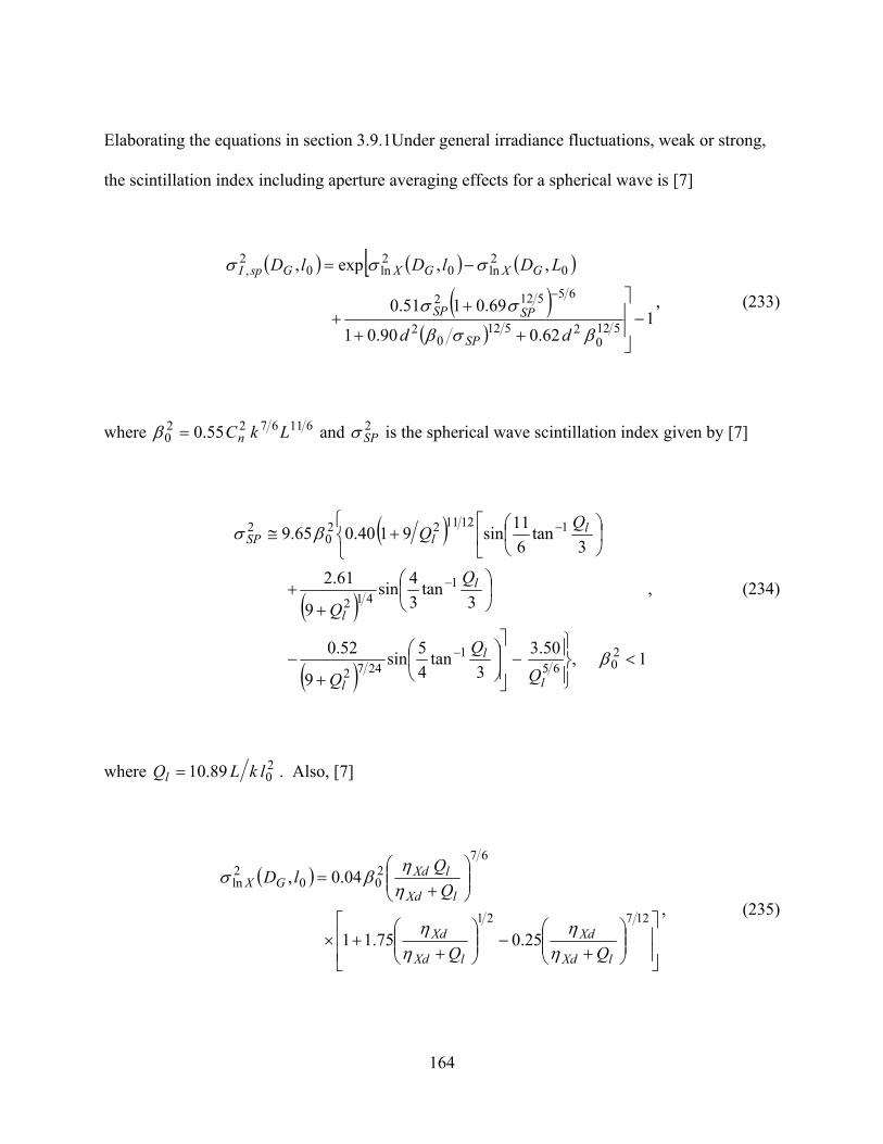
164

Elaborating the equations in section 3.9.1Under general irradiance fluctuations, weak or strong,

the scintillation index including aperture averaging effects for a spherical wave is [7]

( ) ( ) ( )[( )

( )1

62.090.01

69.0151.0

,,exp,

5120

25120

2

655122

02ln0

2ln0

2,

−⎥⎥

⎦

⎤

++

++

−=

−

βσβ

σσ

σσσ

dd

LDlDlD

SP

SPSP

GXGXGspI

, (233)

where 61167220 55.0 LkCn=β and 2

SPσ is the spherical wave scintillation index given by [7]

( )

( )

( )1,50.3

3tan

45sin

9

52.0

3tan

34sin

9

61.2

3tan

611sin9140.065.9

2065

12472

1412

11211220

2

<⎪⎭

⎪⎬⎫

−⎥⎥

⎦

⎤⎟⎠

⎞⎜⎝

⎛

+−

⎟⎠

⎞⎜⎝

⎛

++

⎩⎨⎧

⎢⎣

⎡⎟⎠

⎞⎜⎝

⎛+≅

−

−

−

β

βσ

l

l

l

l

l

llSP

QQ

Q

Q

Q

QQ

, (234)

where 2089.10 lkLQl = . Also, [7]

( )

⎥⎥⎦

⎤

⎢⎢⎣

⎡⎟⎟⎠

⎞⎜⎜⎝

⎛+

−⎟⎟⎠

⎞⎜⎜⎝

⎛+

+×

⎟⎟⎠

⎞⎜⎜⎝

⎛+

=

12721

67200

2ln

25.075.11

04.0,

lXd

Xd

lXd

Xd

lXd

lXdGX

QQ

QQ

lD

ηη

ηη

ηη

βσ

, (235)

165

( )

⎥⎥⎦

⎤

⎢⎢⎣

⎡⎟⎟⎠

⎞⎜⎜⎝

⎛+

−⎟⎟⎠

⎞⎜⎜⎝

⎛+

+×

⎟⎟⎠

⎞⎜⎜⎝

⎛+

=

127

0

021

0

0

67

0

0200

2ln

25.075.11

04.0,

lXd

Xd

lXd

Xd

lXd

lXdGX

QQ

QQ

LD

ηη

ηη

ηη

βσ

, (236)

612020.01

56.8

lX

Qβη

+= , (237)

6120

22 20.018.0156.8

02.01 lX

XXd

Qdd βηη

η++

=+

= , (238)

610

200

20

0

0

00

20.018.056.856.8

lXd

XdXd

QQQdQQ

QQ

βηη

η+++

=+

= , (239)

20

0

2 64,4 Lk

LQL

kDd G π

== . (240)

166

APPENDIX B HANKEL TRANSFORM OF MCF: b = 5/3

167

The integral to be solved is


350 ∫∞

−= (241)

The Bessel function can be represented by an infinite series [70]

( ) ( ) ( )( )∑

∞

= +Γ−

=0

2

0 1!21

k

kk

kkbbJ ρρ (242)

where rb π2= . Substituting this into (241)

( ) ( )( )

( ) ρρρρπ dakk

bIrS k

kk

kk2

0

35

02

2

0 exp21!

12 ∫∑∞∞

=−

+Γ

−= (243)

Working on only the integral

( ) ρρρ da k 12

0

35exp +∞

∫ − (244)

The exponent can be rewritten as ⎟⎠⎞

⎜⎝⎛ +=+

53

56

3512 kk and the integral is then

168

( )( ) ρρρ dak

53

56

35

0

35exp+∞

∫ − (245)

Making a substitution

du

ad

au

daduaulet

323

5

53

323535

1ρ

ρρ

ρρρ

=⎟⎠⎞

⎜⎝⎛=→

==

(246)

The integral becomes

( )∫∫

∞−

+∞−

+

⎟⎠⎞

⎜⎝⎛=⎟

⎠⎞

⎜⎝⎛

0156

35

53

56

032

35

53

56

11 duaua

eaudu

ae

au u

ku

k

ρ (247)

The like terms are collected

( )

∫∞

−−+−+−

0

156

53

56

15615

35

6

53 dueuuaaa ukk

(248)

The terms are then arranged in the form of a gamma function integral

( )

∫∞

−−+−++−

0

11518

56

15615

35

6

53 dueua ukk

(249)

169

Using the definition of the gamma function [70]

( ) ∫∞

−−=Γ0

1 dtetz tz (250)

(248) becomes

( ) ( )⎟

⎠⎞

⎜⎝⎛ +Γ

+−1

56

53 15

185

6ka

k (251)

Substituting back into (243) yields

( ) ( )( )

( ) ( )⎟⎠⎞

⎜⎝⎛ +Γ

+Γ

−=

+−∞

=∑ 1

56

53

21!12 15

185

6

02

2

0 kakk

bIrSk

kk

kkπ (252)

Rearranging terms yields

( ) ( ) ( )

( )1

156

4!

1

5

6

0 56

2

05

6 +Γ

⎟⎠⎞

⎜⎝⎛ +Γ

⎟⎠

⎞⎜⎝

⎛

−= ∑

∞

= k

k

ak

bIa

rSk

k

kkπ (253)

In its current state, the infinite sum has no closed form. A closer look reveals the sum has the

functional form of an exponential, if the ratio of gamma functions were unity [70]

170

x

k

ke

kx

=∑∞

=0 !. (254)

Assuming the functional form of an exponential, a numerical approximation was made

( ) ( )

( ) ⎟⎟⎟

⎠

⎞

⎜⎜⎜

⎝

⎛−

≈+Γ

⎟⎠⎞

⎜⎝⎛ +Γ

⎟⎠

⎞⎜⎝

⎛

−∑∞

= 56

2

0 56

2

4*9.0exp92.0

1

156

4!

1

a

bk

k

ak

b

kk

kk. (255)

The approximation has less than 5% error in area under the curve and a mean square error less

than 4105 −× .

(253) reduces to

( )⎟⎟⎟

⎠

⎞

⎜⎜⎜

⎝

⎛−=

56

2

05

64*9.0

exp5

692.0a

bIa

rS π (256)

Substituting for b

( ) ( )⎟⎟⎟

⎠

⎞

⎜⎜⎜

⎝

⎛−=

56

2

05

64*9.0

2exp5

692.0a

rIa

rS ππ (257)

171

Resulting in

( ) ( )⎟⎟⎟

⎠

⎞

⎜⎜⎜

⎝

⎛−=

56

2

560

9.0exp47.3

a

r

a

IrS π (258)

172

APPENDIX C CHARACTERISTIC FUNCTION

173

First we calculate the corresponding characteristic function for the PDF of irradiance,

( ) ( )∫∞

∞−

==Φ dInIPe jIi

Ij

jnωω (259)

( ) ∫∞

−=Φ0

1 dIeen

jjj

j

nIIi

jI

λω

λω . (260)

We make the change of variable jIx −= and the function is now in the common form of a

Fourier transform

( ) ∫∞−

−=Φ01 dxee

nj

j

nxxi

jI

λω

λω . (261)

Using a Fourier transform table we get

( )j

I nij λωω

−=Φ

11 . (262)

For the total irradiance, the convolution of M PDFs equals the product of M characteristic

functions. We therefore multiply M characteristic functions

174

( ) ∏= −

=ΦM

j jI ni1 1

1λω

ω . (263)

A partial fraction expansion is done to change the product to a sum. The function can be

rewritten as follows:

∑∏ =

=

−=

−

=M

j j

jM

jj

niA

niF

1

1

11

1)(λω

λωω , (264)

where ( ) ( )jin

FniA jjλ

ωωλω 11 =×−= .

We further derive jA

( )⎟⎟⎟⎟⎟

⎠

⎞

⎜⎜⎜⎜⎜

⎝

⎛

−

−=

∏=

M

mm

jj

niniA

11

11λω

λω (265)

( )[ ]

⎟⎟⎟⎟⎟⎟⎟

⎠

⎞

⎜⎜⎜⎜⎜⎜⎜

⎝

⎛

−−

−=

∏≠=

=

M

jmm

mjm

jj

nininiA

111

11λωλω

λω (266)

175

jin

M

jmm

m

j

niA

λω

λω

111

1

=≠=∏ −

= (267)

∏≠=

−

= M

jmm j

mjA

11

1

λλ

. (268)

Substituting into (264)

( ) ( ) ∑∏=

≠=

−−

==ΦM

j jM

jmm j

mI ni

F1

1

11

1

1λω

λλ

ωω (269)

To get the resulting PDF of irradiance, we must invert the characteristic function,

( ) ( ) ωωπ

ω denIP Ii∫∞

∞−

− Φ==21n (270)

and substituting we get

176

( ) ωλωπ

ω dni

AenIP

M

j j

jIi∫ ∑∞

∞− =

−

−==

1121n . (271)

We make the change of variable ω−=x and the function is now in the common form of a

Fourier transform

( ) dxnix

AenIP

M

j j

jixI∫ ∑∞

∞− = +==

1121

λπn . (272)

Rearranging and interchanging the order of integration and summation,

( ) dxixn

enA

nIPj

ixIM

j j

j∫∑∞

∞−= +==

λπλ 11

21

1n . (273)

Using a Fourier transform table we get

( ) ∞≤≤== ∑=

− IenA

nIPM

j

nI

j

j j 01

λ

λn . (274)

The ratio jjA λ can be further simplified, starting with jA

177

( ) ( )∏∏∏

≠=

≠=

≠=

−

−=

−=⎟

⎟⎠

⎞⎜⎜⎝

⎛−=

M

jmm mj

jM

jmm mj

j

M

jmm j

mjA

111

1

111

λλλ

λλλ

λλ

. (275)

Excluding the jm = term in the product results in M-1 products being formed, therefore

( )∏≠=

−

−=

M

jmm mj

MjjA

1

1 1λλ

λ (276)

and

( )∏

≠=

−

−

= M

jmm

mj

Mj

j

jA

1

2

λλ

λλ

. (277)

178

APPENDIX D INTERPRETING POWER METER OUTPUT

179

A decibel (dB) is a unit used to express relative differences in signal strength. A decibel is

expressed as the base 10 logarithm of the ratio of the power of two signals

⎟⎟⎠

⎞⎜⎜⎝

⎛=

2

110log10

PP

dB . (278)

A decibel referenced to one milliwatt (dBm) is the ratio of the input power (in Watts) to 1mW

⎟⎟⎠

⎞⎜⎜⎝

⎛=

mWPdBm

1log10 1

10 . (279)

The output of the New Focus power meter can be written as either [81, 82]

⎟⎟⎠

⎞⎜⎜⎝

⎛=

Z

OPTLOG P

PdBmVV 10log10*50 (280)

( )ZOPTLOG DDdBmVV −= 50 (281)

where “D” denotes the power in decibels as opposed to “P” which expresses power in Watts.

DOPT is the optical power in decibels above a reference level and DZ is the equivalent intercept

power relative to the same level.

180

In order to convert the output of the New Focus 2101 power meter to true measured power, DZ

must be calculated. Typically, one would take a measurement of a known source at the

wavelength of interest and use that to calculate the intercept power. However, for this case we

will use the approximate value of 2dBm of input power at 920nm corresponding to a 3.5V

output, as stated in the users manual [82]. The user’s manual also estimates a 2dB drop in

response at a wavelength of approximately 532nm.

( )

dBmD

DdBdBmdBmVV

Z

Z

70

22505.3

−=

−−= (282)

DOPT is the optical power as referenced to 1mW; therefore it is related to the input power by

⎟⎟⎠

⎞⎜⎜⎝

⎛=

mWP

D inOPT 1

log10 10 (283)

Substituting for DOPT in (280) above, the input optical is related to the output voltage by

[ ]WV

P LOGin ⎟

⎠

⎞⎜⎝

⎛ −=

5.05.3

^10 (284)

The minimum detectable power of the detection system can be calculated. The digitizer has 24

bits of resolution and was operated over a range of -5V to +5V. The smallest detectable voltage

is given by

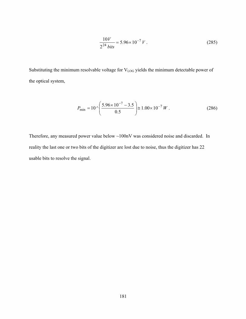
181

VbitsV 7

24 1096.52

10 −×= . (285)

Substituting the minimum resolvable voltage for VLOG yields the minimum detectable power of

the optical system,

WP 77

min 1000.15.0

5.31096.5^10 −−

×≅⎟⎟⎠

⎞⎜⎜⎝

⎛ −×= . (286)

Therefore, any measured power value below ~100nV was considered noise and discarded. In

reality the last one or two bits of the digitizer are lost due to noise, thus the digitizer has 22

usable bits to resolve the signal.

182

APPENDIX E NUMERICAL INACCURACIES OF NEW PDF AT LOW IRRADIANCE

183

Recall the PDF of irradiance derived herein,

( ) ∑∑==

⎟⎟

⎠

⎞

⎜⎜

⎝

⎛=

N

k kjk

kM

j j

j IKBA

IP1

01

22γλγλ

, (287)

where

( )∏

≠=

−

−

= M

jmm

mj

Mj

jA

1

1

λλ

λ,

( )∏≠=

−

−

= N

knn

nk

Nk

kB

1

1

γγ

γ. (288)

At low values of irradiance the new PDF exhibits oscillations, implying convergence issues. It is

understood that a finite sum will always converge, however the finite sum representing the PDF

of irradiance should be monotonically decreasing in the tails. Initially, the oscillations in the

PDF were thought to be from numerical inaccuracies in the K0 Bessel function. However,

implementation of the PDF in both Mathematica and Matlab yielded identical results. Another

possible cause of the convergence issues lies is the method of selecting of the λ’s and γ’s. It has

been observed that different methods of selecting the λ’s and γ’s lead to different convergence

results in the PDF. The oscillations in the low tail become more prevalent as the number of λ’s

used is increased. As the number of λ’s is increased the spacing between subsequent λ’s is

decreased, see Figure 13. The PDF has a finite product of the differences of the λ’s in the

denominator and is therefore severely dependent on the differences of λ’s. It is believed the

approximations made in the eigenfunctions and eigenvalues of the KL expansion introduce a

small error. This error starts to manifest when the difference of many eigenvalues are multiplied

184

together. Small errors in the λ’s and γ’s are also exacerbated by the K0 Bessel function for small

values of irradiance. For small arguments of the Bessel function it has an asymptotic behavior

proportional to the negative logarithm [70]

( ) ( ) +→− 0,ln~0 zzzK (289)

whereas for large arguments, the Bessel function approaches zero exponentially. The

oscillations can also be brought about by changing the sampling interval rΔ . As the sampling

interval is decreased, the λ’s become more similar and the oscillations begin at lower values of

M. The oscillations appear to be less dependent upon the γ’s.

The figures below are a typical example of the oscillations as the number of λ’s is changed and

all other parameters are held constant.

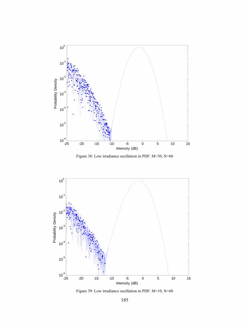
185

-25 -20 -15 -10 -5 0 5 10 1510-6

10-5

10-4

10-3

10-2

10-1

100

Intensity (dB)

Pro

babi

lity

Den

sity

Figure 38: Low irradiance oscillation in PDF: M=30, N=60

-25 -20 -15 -10 -5 0 5 10 1510-6

10-5

10-4

10-3

10-2

10-1

100

Intensity (dB)

Pro

babi

lity

Den

sity


186

-25 -20 -15 -10 -5 0 5 10 1510-6

10-5

10-4

10-3

10-2

10-1

100

Intensity (dB)

Pro

babi

lity

Den

sity


187

LIST OF REFERENCES

[1] J. Hecht, "Laser Evolution," in SPIE Professional. vol. 4 Bellingham, WA: SPIE, 2009, p. 40.

[2] D. M. Boroson, A. Biswas, and B. L. Edwards, "MLCD: overview of NASA's Mars laser communications demonstration system," in Photonics West: LASE, San Jose, CA.

[3] V. I. Tatarskii, Wave propagation in a turbulent medium. Newe York: Dover Publications, 1967.

[4] V. I. Tatarskii, The Effects of the Turbulent Atmosphere on Wave Propagation: Jerusalem: Israel Program for Scientific Translations, 1971.

[5] L. B. Stotts, B. Stadler, D. Hughes, P. Kolodzy, A. Pike, D. W. Young, J. Sluz, J. Juarez, B. Graves, D. Dougherty, J. Douglass, and T. Martin, "Optical communications in atmospheric turbulence," in Free-Space Laser Communications IX, San Diego, CA, USA, 2009, pp. 746403-17.

[6] M. Al Naboulsi, H. Sizun, and F. de Fornel, "Propagation of optical and infrared waves in the atmosphere," in Wave Propagation and Remote Sensing, Boulder, CO, USA, 2005.

[7] L. C. Andrews and R. L. Phillips, Laser beam propagation through random media, 2nd ed. Bellingham, Wash.: SPIE Press, 2005.

[8] J. S. Bendat and A. G. Piersol, Random data : analysis and measurement procedures, 3rd ed. New York: Wiley, 2000.

[9] A. Papoulis and S. U. Pillai, Probability, random variables, and stochastic processes, 4th ed. Boston: McGraw-Hill, 2002.

[10] J. L. Lumley and H. A. Panofsky, The structure of atmospheric turbulence. New York,: Interscience Publishers, 1964.

[11] L. C. Andrews, R. L. Phillips, and C. Y. Hopen, Laser beam scintillation with applications. Bellingham, Wash.: SPIE Press, 2001.

[12] R. M. Bethea and R. R. Rhinehart, Applied engineering statistics. New York: M. Dekker, 1991.

[13] T. W. Beck, T. J. Housh, J. P. Weir, J. T. Cramer, V. Vardaxis, G. O. Johnson, J. W. Coburn, M. H. Malek, and M. Mielke, "An examination of the Runs Test, Reverse Arrangements Test, and modified Reverse Arrangements Test for assessing surface EMG signal stationarity," Journal of Neuroscience Methods, vol. 156, pp. 242-248, 2006.

[14] L. C. Andrews and R. L. Phillips, Mathematical techniques for engineers and scientists. Bellingham, Wash.: SPIE Press, 2003.

[15] D. Freedman, "Statistics," 2nd ed New York: Norton, 1991, pp. 29 - 46. [16] D. W. Scott, "On optimal and data-based histograms," Biometrika, vol. 66, pp. 605-610,

December 1, 1979 1979. [17] D. Freedman and P. Diaconis, "On the histogram as a density estimator:L2 theory,"

Probability Theory and Related Fields, vol. 57, pp. 453-476, 1981. [18] J. S. Accetta and D. L. Shumaker, "The Infrared and electro-optical systems handbook."

vol. 2 Ann Arbor, Mich.; Bellingham, Wash.: Infrared Information Analysis Center; SPIE Optical Engineering Press, 1993, pp. 169-173.

[19] J. W. Strohbehn and S. F. Clifford, Laser beam propagation in the atmosphere. Berlin ; New York: Springer-Verlag, 1978.

188

[20] H. T. Yura, C. C. Sung, S. F. Clifford, and R. J. Hill, "Second-order Rytov approximation," J. Opt. Soc. Am., vol. 73, pp. 500-502, 1983.

[21] R. J. Hill and S. F. Clifford, "Modified spectrum of atmospheric temperature fluctuations and its application to optical propagation," J. Opt. Soc. Am., vol. 68, pp. 892-899, 1978.

[22] C. E. Coulman, "A quantitative treatment of solar ‘seeing’ I," Solar Physics, vol. 7, p. 22, 1969.

[23] R. S. Lawrence and J. W. Strohbehn, "A survey of clear-air propagation effects relevant to optical communications," Proceedings of the IEEE, vol. 58, pp. 1523-1545, 1970.

[24] E. M. Sparrow, R. B. Husar, and R. J. Goldstein, "Observations and other characteristics of thermals," Journal of Fluid Mechanics Digital Archive, vol. 41, pp. 793-800, 1970.

[25] L. C. Andrews, R. L. Phillips, D. Wayne, T. Leclerc, P. Sauer, R. Crabbs, and J. Kiriazes, "Near-ground vertical profile of refractive-index fluctuations," in Atmospheric Propagation VI, Orlando, FL, USA, 2009, pp. 732402-12.

[26] R. M. Gagliardi and S. Karp, Optical communications. New York: Wiley, 1976. [27] M. E. Gracheva and A. S. Gurvich, "Strong fluctuations in the intensity of light

propagated through the atmosphere close to the earth," Radiophysics and Quantum Electronics, vol. 8, pp. 511–525, 1965.

[28] F. Strömqvist Vetelino, "Fade statistics for a lasercom system and the joint PDF of a gamma-gamma distributed irradiance and its time derivative," in Mathematics. vol. Ph.D Orlando: University of Central Florida, 2006, p. 207.

[29] E. Jakeman and P. Pusey, "A model for non-Rayleigh sea echo," Antennas and Propagation, IEEE Transactions on, vol. 24, pp. 806-814, 1976.

[30] E. Jakeman and P. N. Pusey, "Significance of K Distributions in Scattering Experiments," Physical Review Letters, vol. 40, p. 546, 1978.

[31] D. Lewinski, "Nonstationary probabilistic target and clutter scattering models," Antennas and Propagation, IEEE Transactions on, vol. 31, pp. 490-498, 1983.

[32] L. C. Andrews and R. L. Phillips, "I-K distribution as a universal propagation model of laser beams in atmospheric turbulence," J. Opt. Soc. Am. A, vol. 2, pp. 160-163, 1985.

[33] J. H. Churnside and S. F. Clifford, "Log-normal Rician probability-density function of optical scintillations in the turbulent atmosphere," J. Opt. Soc. Am. A, vol. 4, pp. 1923-1930, 1987.

[34] F. S. Vetelino, C. Young, L. Andrews, and J. Recolons, "Aperture averaging effects on the probability density of irradiance fluctuations in moderate-to-strong turbulence," Appl. Opt., vol. 46, pp. 2099-2108, 2007.

[35] L. C. Andrews, R. L. Phillips, and B. K. Shivamoggi, "Relations of the parameters of the I-K distribution for irradiance fluctuations to physical parameters of the turbulence," Appl. Opt., vol. 27, pp. 2150-2156, 1988.

[36] J. H. Churnside and R. G. Frehlich, "Experimental evaluation of log-normally modulated Rician and IK models of optical scintillation in the atmosphere," J. Opt. Soc. Am. A, vol. 6, pp. 1760-1766, 1989.

[37] T.-i. Wang and J. W. Strohbehn, "Perturbed log-normal distribution of irradiance fluctuations," J. Opt. Soc. Am., vol. 64, pp. 994-999, 1974.

[38] X. Xiao and D. Voelz, "On-axis probability density function and fade behavior of partially coherent beams propagating through turbulence," Appl. Opt., vol. 48, pp. 167-175, 2009.

189

[39] D. A. Dewolf, "Saturation of Irradiance Fluctuations Due to Turbulent Atmosphere," J. Opt. Soc. Am., vol. 58, pp. 461-465, 1968.

[40] M. Nakagami, K. Tanaka, and M. Kanehisa, "The m-Distribution As the General Formula of Intensity Distribution of Rapid Fading," Memoirs of the Faculty of Engineering, Kobe University, vol. 4, pp. 78-125, 19570300 1957.

[41] A. R. Weeks and University of Central Florida. College of Engineering., "An experimental and theoretical analysis of a laser beam propagating through multiple phase screens," University of Central florida, 1987., 1987, pp. vii, 167 leaves, bound.

[42] G. Parry and P. N. Pusey, "K distributions in atmospheric propagation of laser light," J. Opt. Soc. Am., vol. 69, pp. 796-798, 1979.

[43] R. L. Phillips and L. C. Andrews, "Measured statistics of laser-light scattering in atmospheric turbulence," J. Opt. Soc. Am., vol. 71, pp. 1440-1445, 1981.

[44] A. Ishimaru, Wave propagation and scattering in random media. New York; Oxford: IEEE Press; Oxford University Press, 1997.

[45] R. L. Fante, "Electromagnetic beam propagation in turbulent media," Proceedings of the IEEE, vol. 63, pp. 1669-1692, 1975.

[46] A. D. Wheelon, "Skewed distribution of irradiance predicted by the second-order Rytov approximation," J. Opt. Soc. Am. A, vol. 18, pp. 2789-2798, 2001.

[47] H. T. Yura and R. F. Lutomirski, "Irradiance Statistics, Modulation Transfer Function, and Phase Structure Function of an Optical Wave in a Turbulent Medium," Rand Corp. Santa Monica, California 1969.

[48] S. Michael, R. R. Parenti, F. G. Walther, A. M. Volpicelli, J. D. Moores, J. W. Wilcox, and R. Murphy, "Comparison of scintillation measurements from a 5 km communication link to standard statistical models," in Atmospheric Propagation VI, Orlando, FL, USA, 2009, pp. 73240J-7.

[49] J. R. Dunphy and J. R. Kerr, "Scintillation measurements for large integrated-path turbulence," J. Opt. Soc. Am., vol. 63, pp. 981-986, 1973.

[50] G. R. Ochs, R. R. Bergmtan, and J. R. Snyder, "Laser-Beam Scintillation over Horizontal Paths from 5.5 to 145 Kilometers," J. Opt. Soc. Am., vol. 59, pp. 231-234, 1969.

[51] R. J. Hill and R. G. Frehlich, "Probability distribution of irradiance for the onset of strong scintillation," J. Opt. Soc. Am. A, vol. 14, pp. 1530-1540, 1997.

[52] J. H. Churnside and R. J. Hill, "Probability density of irradiance scintillations for strong path-integrated refractive turbulence," J. Opt. Soc. Am. A, vol. 4, pp. 727-733, 1987.

[53] R. A. Elliott, J. R. Kerr, and P. A. Pincus, "Optical propagation in laboratory-generated turbulence," Appl. Opt., vol. 18, pp. 3315-3323, 1979.

[54] J. W. Strohbehn, "Line-of-sight wave propagation through the turbulent atmosphere," Proceedings of the IEEE, vol. 56, pp. 1301-1318, 1968.

[55] E. Jakeman, "On the statistics of K-distributed noise," Journal of Physics A: Mathematical and General, vol. 13, pp. 31-48, 1980.

[56] S. M. Flatté, C. Bracher, and G.-Y. Wang, "Probability-density functions of irradiance for waves in atmospheric turbulence calculated by numerical simulation," J. Opt. Soc. Am. A, vol. 11, pp. 2080-2092, 1994.

[57] R. Dashen, "Distribution of intensity in a multiply scattering medium," Opt. Lett., vol. 9, pp. 110-112, 1984.

190

[58] M. A. Al-Habash, L. C. Andrews, and R. L. Phillips, "Mathematical model for the irradiance probability density function of a laser beam propagating through turbulent media," Optical Engineering, vol. 40, pp. 1554-1562, 2001.

[59] R. L. Phillips and L. C. Andrews, "Universal statistical model for irradiance fluctuations in a turbulent medium," J. Opt. Soc. Am., vol. 72, pp. 864-870, 1982.

[60] L. C. Andrews and R. L. Phillips, "Mathematical genesis of the I-K distribution for random optical fields," J. Opt. Soc. Am. A, vol. 3, pp. 1912-1919, 1986.

[61] D. J. Link, "Phase Statistics for a Lightwave Traveling through Turbulent Media " in College of Engineering. vol. Ph. D Orlando: University of Central Florida, 1985, p. 110.

[62] R. Barakat, "Weak-scatterer generalization of the K-density function with application to laser scattering in atmospheric turbulence," J. Opt. Soc. Am. A, vol. 3, pp. 401-409, 1986.

[63] E. Jakeman and R. J. A. Tough, "Generalized K distribution: a statistical model for weak scattering," J. Opt. Soc. Am. A, vol. 4, pp. 1764-1772, 1987.

[64] J. W. Goodman, "Statistical Properties of Laser Speckle Patterns," in Laser speckle and related phenomena, 2nd ed. vol. 9, J. C. Dainty, Ed. Berlin ; New York: Springer-Verlag, 1984, pp. xv, 342 p.

[65] R. Barakat, "Direct derivation of intensity and phase statistics of speckle produced by a weak scatterer from the random sinusoid model," J. Opt. Soc. Am., vol. 71, pp. 86-90, 1981.

[66] J. W. Strohbehn, T.-i. Wang, and J. P. Speck, "On the probability distribution of line-of-sight fluctuations of optical signals," Radio Sci., vol. 10.

[67] P. Beckmann, Probability in communication engineering. New York: Harcourt, Brace & World, 1967.

[68] L. C. Andrews, R. L. Phillips, C. Y. Hopen, and M. A. Al-Habash, "Theory of optical scintillation," J. Opt. Soc. Am. A, vol. 16, pp. 1417-1429, 1999.

[69] L. C. Andrews, R. L. Phillips, and C. Y. Hopen, "Aperture averaging of optical scintillations: power fluctuations and the temporal spectrum," Waves in Random and Complex Media, vol. 10, pp. 53 - 70, 2000.

[70] L. C. Andrews, Special functions of mathematics for engineers. Bellingham, Wash., USA: SPIE Optical Engineering Press ; Oxford University Press, 1998.

[71] C. C. Heyde, "On a Property of the Lognormal Distribution," Journal of the Royal Statistical Society. Series B (Methodological), vol. 25, pp. 392-393, 1963.

[72] K. Furutsu, "Statistical Theory of Wave Propagation in a Random Medium and the Irradiance Distribution Function," J. Opt. Soc. Am., vol. 62, pp. 240-254, 1972.

[73] J. W. Goodman, Introduction to Fourier optics, 3rd ed. Englewood, Colo.: Roberts & Co., 2005.

[74] M. Girolami, "Orthogonal Series Density Estimation and the Kernel Eigenvalue Problem," Neural Computation, vol. 14, pp. 669-688, 2002.

[75] B. E. A. Saleh, Photoelectron statistics, with applications to spectroscopy and optical communication. Berlin ; New York: Springer-Verlag, 1978.

[76] E. Vanmarcke, Random fields, analysis and synthesis. Cambridge, Mass.: MIT Press, 1983.

[77] T.-i. Wang, G. R. Ochs, and S. F. Clifford, "A saturation-resistant optical scintillometer to measure C2n," J. Opt. Soc. Am., vol. 68, pp. 334-338, 1978.

191

[78] Scintec, "Scintec Boundary Layer Scintillometer User Manual," Version 1.49 ed, December 2008.

[79] S. F. Clifford, G. R. Ochs, and R. S. Lawrence, "Saturation of optical scintillation by strong turbulence," J. Opt. Soc. Am., vol. 64, pp. 148-154, 1974.

[80] Scintec, "Scintec Surface Layer Scintillometer User Manual," Version 1.34 ed, September 2008.

[81] Analog_Devices, "AD8304: 160 dB Logarithmic Amplifier User's Guide," Rev. A ed, Aug 2002.

[82] New_Focus, "High-Dynamic-Range Power Sensors Models 2101 & 2103 User's Guide," 210018 Rev.C ed, June 2010.

The Pdf Of Irradiance For A Free-space Optical ...

Documents

Transcript of The Pdf Of Irradiance For A Free-space Optical ...