NBER WORKING PAPER SERIES

THE ORIGINS OF EARLY CHILDHOOD ANTHROPOMETRIC PERSISTENCE

Daniel L. MillimetRusty Tchernis

Working Paper 19554http://www.nber.org/papers/w19554

NATIONAL BUREAU OF ECONOMIC RESEARCH1050 Massachusetts Avenue

Cambridge, MA 02138October 2013

This study was conducted by Georgia State University and Southern Methodist University under acooperative agreement with the U.S. Department of Agriculture, Economic Research Service, Foodand Nutrition Assistance Research Program (agreement no. 58-5000-0-0080). The views expressedhere are those of the authors and do not necessarily reflect those of the USDA or ERS. The authorsare grateful to Chris Ruhm for helpful comments and Lorenzo Almada for excellent research assistance.The views expressed herein are those of the authors and do not necessarily reflect the views of theNational Bureau of Economic Research.

NBER working papers are circulated for discussion and comment purposes. They have not been peer-reviewed or been subject to the review by the NBER Board of Directors that accompanies officialNBER publications.

© 2013 by Daniel L. Millimet and Rusty Tchernis. All rights reserved. Short sections of text, not toexceed two paragraphs, may be quoted without explicit permission provided that full credit, including© notice, is given to the source.

The Origins of Early Childhood Anthropometric PersistenceDaniel L. Millimet and Rusty TchernisNBER Working Paper No. 19554October 2013JEL No. C23,I12,I18

ABSTRACT

Rates of childhood obesity have increased dramatically in the last few decades. Non-causal evidencesuggests that childhood obesity is highly persistent over the life cycle. However little in known aboutthe origins of this persistence. In this paper we attempt to answer three questions. First, how do anthropometricmeasures evolve from birth through primary school? Second, what is the causal effect of past anthropometricoutcomes on future anthropometric outcomes? In other words, how important is state dependencein the evolution of anthropometric measures during the early part of the life cycle. Third, how importantare time-varying and time invariant factors in the dynamics of childhood anthropometric measures?We find that anthropometric measures are highly persistent from infancy through primary school.Moreover, most of this persistence is driven by unobserved, time invariant factors that are determinedprior to birth, consistent with the so-called fetal origins hypothesis. As such, policy interventions designedto improve child anthropometric status will only have meaningful, long-run effects if these time invariantfactors are altered. Unfortunately, future research is needed to identify such factors, although evidencesuggests that maternal nutrition may play an important role.

Daniel L. MillimetDept of EconomicsBox 0496SMUDallas, TX 75275-0496millimet@smu.edu

Rusty TchernisDepartment of EconomicsAndrew Young School of Policy StudiesGeorgia State UniversityP.O. Box 3992Atlanta, GA 30302-3992and NBERrtchernis@gsu.edu

1 Introduction

The rise in childhood obesity in the U.S. is well chronicled. Moreover, strong evidence suggests that childhood obesity

is highly persistent over the life cycle. However little in known about the origins of this persistence. In this paper

we attempt to answer three questions. First, how do weight and height evolve from birth through primary school?

Second, what is the causal effect of past weight and height status on the future weight and height of children? In

other words, how important is state dependence in the evolution of anthropometric measures during the early part of

the life cycle. Third, how important are time-varying and time invariant factors in the dynamics of childhood weight

and height?

These are important public health questions of vital importance to policymakers as the prevalence of obese

adolescents has tripled in the last thirty years; it has more than doubled for younger children. Defined as having an

age- and sex-adjusted body mass index (BMI) above the 95th percentile of the reference distribution, the prevalence

of obese children increased from 5% to 12.4% for 2-5 year old children and from 5% to 17.6% for 12 to 19 year-olds

between 1976 and 2006 (Ogden et al. 2008). In addition, vast differences in the time trends of BMI increases have

been documented: the incidence of obesity among white girls aged 12-19 has increased from 7.4% to 14.5% between

1988 and 2006, whereas the corresponding figures for African-American girls are 13.2% and 27.7% (Ogden et al.

2002; Ogden et al. 2008). Deckelbaum and Williams (2001, p. 242S) conclude that “childhood obesity is increasing

at epidemic rates, even among pre-school children...” More recently, Brisbois et al. (2012, p. 347) state: “Obesity is

considered to be a worldwide epidemic with little evidence that its incidence is declining or that it has even reached

a plateau.”

While there exists some evidence that childhood obesity rates may have begun to recede in the U.S., concern over

childhood obesity remains high due to the well-documented consequences of obesity and the lack of understanding

pertaining to the turnaround.1 Obesity burdens individuals with severe physical, economic, and emotional suffering,

and puts children and adolescents at risk for a number of health problems such as those affecting cardiovascular

health, the endocrine system, and mental health (Deckelbaum and Williams 2001; Krebs and Jacobson 2003). Dietz

and Gortmaker (2001) note that 60% of overweight children aged five to ten years old have at least one associated

cardiovascular disease risk factor.

Perhaps the largest cost of childhood obesity comes from its impact on adult obesity. Currently, 60% of the total

U.S. population is overweight or obese and 50% is expected to be obese in 2030 at the current rate (Dor et al. 2010).

Walpole et al. (2012) calculate that North America accounts for 34% of the total human biomass in the world despite

containing only 6% of the world population. Moreover, the authors estimate that if the entire world had the same

BMI distribution as the U.S., this would be equivalent to an additional 935 million people in the world of average

BMI. Finkelstein and Zuckerman (2007) report that if the childhood obesity epidemic continues unabated at the

current rate, as many as 30-40% of the US population will develop Type 2 Diabetes during their lifetime. Mocan

and Tekin (2011) document the links between adult obesity and lower wages, productivity, and self-esteem. In the

U.S., the total cost attributable to obesity was over $75 billion in 2000 according to Finkelstein et al. (2004). More

1See http://www.nytimes.com/2013/08/07/health/broad-decline-in-obesity-rate-seen-in-poor-young-

children.html?pagewanted=all.

1

recent estimates put the cost over $200 billion (Cawley and Meyerhoefer 2012).

While the changes in childhood obesity rates across cohorts, as well as the consequences of these increases, are

well-documented, much less is known about how anthropometric measures of children evolve over the life cycle. A

growing literature has investigated persistence in anthropometric outcomes in a non-causal framework, stressing the

correlation in outcomes over time.2 Whitaker et al. (1997) found that the probability of an overweight six year-old

child becoming an obese adult is 50% compared to 10% for a non-overweight child. In addition, the risk of becoming

obese in adulthood is exacerbated by having an obese parent. Eriksson et al. (2001) found that individuals were

three times more likely to be obese as an adult if they had a BMI greater than 16, as opposed to below 14.5, at age

seven. Nader et al. (2007) find that children who were overweight prior to the age of five are five times as likely to

be overweight at 12 relative to children who were not overweight prior to the age of five.

Freedman et al. (2001) also report a strong relationship between overweight status in childhood and adult BMI.

However, most striking is that obese adults who were overweight prior to age eight have a much higher BMI than

individuals suffering from adult onset obesity (41 versus 35). In a later study, Freedman et al. (2005) document

significant differences in the transmission of BMI from childhood to adulthood along racial lines. Gable et al. (2008)

analyze the relationship between socioeconomic status, overweight persistence, and school outcomes. The authors

find that family socioeconomic status is predictive of both the probability of a child being overweight and the

probability of persistence of overweight status. Van Cleave et al. (2010) analyze changes in the prevalence of obesity

and other chronic conditions (e.g., asthma, other physical and learning conditions). The authors find that prevalence

of obesity is increasing and is highly persistent over time. Conversely, many children with chronic conditions at ages

two through eight did not have the condition six years later. Finally, Millimet and Tchernis (2013) assess persistence

during infancy and primary school, documenting a significant increase in persistence upon entry into primary school.

Deckelbaum and Williams (2001, p. 239S) conclude: “Disturbingly, obesity in childhood, particularly in adolescence

is a key predictor for obesity in adulthood.” Similarly, Dietz and Gortmaker (2001, p. 340) state: “The best evidence

suggests that the majority of overweight adolescents go on to be overweight adults.”

We build on this prior literature in an attempt to uncover the origins of the persistence in anthropometric

measures. Specifically, we revisit the question of persistence in early childhood health outcomes and investigate

the relative importance of state dependence (i.e., a causal effect of past anthropometric status on future status),

unobserved heterogeneity (i.e., unobserved genetic or environmental risk factors), and observed heterogeneity (i.e.,

commonly measured risk factors) on this persistence. We then ask whether the origins of anthropometric persistence

vary by age, race, gender, or socioeconomic status. Our analysis is fundamentally important for researchers as well

as policymakers. If obesity has its origins early in life and is persistent over time, then early intervention is preferable

to waiting until adolescence or beyond.3 However, and perhaps most importantly, if persistence is due to persistent

2 Iughetti et al. (2008) provide an excellent review.3For instance, an article in the New York Times on March 22, 2010 states that some evidence now suggests that chil-

dren may become entrenched “on an obesity trajectory” even before kindergarten; however, the evidence is not “ironclad”

(http://www.nytimes.com/2010/03/23/health/23obese.html.). Public health officials tend to advocate school-based reforms in light

of the near universal enrollment, yet others stress the importance of preschool interventions (e.g., Frisvold and Giri 2011; Dietz and

Gortmaker 2001; Davis and Christoffel 1994). Eriksson et al. (2001, p. 735) conclude that “obesity is initiated early in life.”

2

underlying factors rather than state dependence, then only by altering these factors can children be moved to a

different trajectory.

To examine these fundamental questions, we estimate dynamic regression models using data from the Early Child-

hood Longitudinal Survey — Kindergarten Cohort (ECLS-K). The ECLS-K is a nationally representative longitudinal

survey of children entering kindergarten in Fall 1998. In addition to providing information on birthweight, anthro-

pometric data is collected at several points in time between kindergarten and eighth grade. We then supplement this

analysis by examining data from the Early Childhood Longitudinal Survey — Birth Cohort (ECLS-B). The ECLS-B

is a nationally representative longitudinal survey of children born in the U.S. in 2001. Information is provided on

these children at ages 9 months, two years, four years, and five years. Thus, the ECLS-B sample allows for a more

refined examination of anthropometric trajectories prior to kindergarten entry.

The analysis leads to two salient conclusions. First, weight, height, and BMI are highly persistent starting in early

infancy. Second, the vast majority of persistence is attributable to time invariant characteristics of children. This

finding is of critical importance as it implies that the only interventions that will have a substantive, long-run effect

on a child’s anthropometric status are those that alter these salient, time invariant attributes. Thus, current policy

interventions may, at best, have a marginal impact in the short-run and, at worst, be destined to fail (see, e.g., Davis

and Gebremariam (2010)). Moreover, while it is difficult to say what these critical, time invariant attributes are

given the data at hand, we find some evidence that fetal nutrition — as proxied by mother’s pre-pregnancy weight and

weight gain during pregnancy, gestation age, birth status (singleton, twin, or higher order birth), and birthweight

— impacts the evolution of anthropometric measures over the early life cycle. However, unobserved, time invariant

attributes play a much more prominent role.

The notion that attributes determined at or shortly after birth, and thus time invariant over the life of an

individual, play a dominant role in the evolution of obesity is consistent with the strong evidence in economics and

elsewhere on the so-called fetal origins hypothesis (see, e.g., Almond and Currie 2011).4 The fetal origins hypothesis,

also referred to as the thrifty phenotype hypothesis or Barker’s hypothesis (due to Barker’s original publication in

1992), posits long-run effects of conditions in utero during critical periods of development through “programmed”

changes in the physiology and metabolism of individuals (Barker 1997). An article in Time on September 22, 2010

summarizes5:

“[P]ioneers assert that the nine months of gestation constitute the most consequential period of our lives,

permanently influencing the wiring of the brain and the functioning of organs such as the heart, liver

and pancreas. The conditions we encounter in utero, they claim, shape our susceptibility to disease, our

appetite and metabolism, our intelligence and temperament. In the literature on the subject, which has

exploded over the past 10 years, you can find references to the fetal origins of cancer, cardiovascular

disease, allergies, asthma, hypertension, diabetes, obesity, mental illness – even of conditions associated

with old age like arthritis, osteoporosis and cognitive decline.”

4While the findings here are consistent with the fetal origins hypothesis, we cannot eliminate other possible explanations for what

these salient, unobserved attributes entail.5 See http://www.time.com/time/magazine/article/0,9171,2021065,00.html.

3

Our analysis is consistent with this view, the implications of which are quite profound. If correct, the most efficient

interventions to curb obesity may need to start prior to childbirth. Deckelbaum &Williams (2001, p. 239S) conclude:

“Novel approaches in the prevention and treatment of childhood overweight and obesity are urgently

required. With the strong evidence that a lifecycle perspective is important in obesity development and

its consequences, consideration must be focused on prevention of obesity in women of child-bearing age,

excessive weight gain during pregnancy, and the role of breast-feeding in reducing later obesity in children

and adults. Consideration must be given to family behavior patterns, diet after weaning, and the use of

new methods of information dissemination to help reduce the impact of childhood obesity worldwide.”

The remainder of the paper is organized as follows. Section 2 provides a brief overview of the prior literature.

Section 3 presents the empirical methodology and data overview. Section 4 discusses the results and their implications.

Section 5 concludes.

2 Related Literature

In addition to the literature already discussed pertaining to the correlations between childhood weight status and

adult obesity, two other prior strands of literature are worth discussing. The first strand includes investigations

on the persistence in health among adolescents and adults in a causal framework. For example, Halliday (2008)

investigates persistence in self-reported health status among white adults age 22-60 using data from the PSID and

allows the parameters of the model to vary. The results suggest that the degree of state dependence — the causal

effect of past states on one’s current state — in health is modest for half the population, yet it explains much of the

observed persistence in health for the other half. Ham et al. (2013) analyze persistence in bulimia nervosa in young

women. The authors find a substantial role for state dependence in the persistence of bulimia nervosa, thus justifying

the importance of early intervention. Our analysis follows the logic of these studies.

The second strand focuses explicitly on the fetal origins hypothesis. As stated earlier, beginning with Barker’s

work, there is a strong belief that in utero events may determine whether a fetus ends up on an “obesity trajectory.”

Deckelbaum & Williams (2001, p. 239S) note that “emerging data suggest associations between the influence of

maternal and fetal factors during intrauterine growth and growth during the first year of life, on risk of later

development of adult obesity and its comorbidities.” More recently, Brisbois et al. (2012, p. 347) state: “Based on

recent evidence, early-life experiences in utero and postnatal influences may induce permanent changes in physiologic

function that programme the long-term regulation of energy balance. This subsequently may adversely impact obesity

risk in later life.”

Which factors may induce such permanent changes in order to set a fetus upon an “obesity trajectory” is the

subject of on-going research. While initial hypotheses focused on undernutrition and oxygen supply, additional

factors such as maternal BMI, maternal weight gain, maternal smoking, gestational diabetes requiring insulin, and

postnatal characteristics such as breastfeeding and the timing of introduction to solid foods are also found to be

important (Dietz 1997; Deckelbaum and Williams 2001; Brisbois et al. 2012).

4

Within this literature, studies have also focused on the identification of early life physical indicators of predispo-

sition to future obesity. Preliminary results suggest that birthweight, length, and gestation age at birth alone are not

strong predictors. Instead, there are complex interactions between these measures, along with other measures such

as head circumference, that matter. For example, a fetus born prematurely and, as a result, with low birthweight

and length is not likely to be at greater risk of future obesity as long as the fetus’ measurements are in proportion

and within ‘normal’ ranges given its gestation age. On the other hand, a fetus born with disproportionate physical

measurements suggests a greater risk (Barker 1997; Sayer et al. 1997; Godfrey and Barker 2001; Brisbois et al.

2012).

3 Empirics

3.1 Methodology

We assess the extent and origins of persistence using a dynamic regression framework. This approach allows for

the decomposition of persistence into various components reflecting state dependence, observed heterogeneity, and

unobserved heterogeneity.

The simplest estimating equation is

= −1 + = 1 ; = 1 (1)

where is a measure of weight status for child at time , is a mean zero error term, and must be at least two

(given observability of the initial observation, 0). Here, reflects the overall level of persistence as it captures the

entire association between past and current anthropometric status. To decompose this overall persistence, we next

incorporate observed heterogeneity into the model

= −1 + + + = 1 ; = 1 (2)

where is a vector of observed, time-varying attributes of child at time and is a vector of observed, time

invariant attributes of child . The change in the estimate of from (1) to (2) reflects the portion of persistence

attributable to persistent, observed heterogeneity. Finally, we include observed time-varying heterogeneity and all

sources (observed and unobserved) of time-invariant heterogeneity into the model

= −1 + + + = 1 ; = 1 (3)

where is a child-specific fixed effect. In (3) reflects the degree of state dependence as it captures the causal effect

of past weight status on current weight status. The child-specific fixed effect, , reflects persistence in child anthro-

pometric measures due to persistent observed and unobserved, child-specific heterogeneity (such as time invariant

environmental and genetic factors). In such models, represents the contemporaneous effects of the observed, time

varying regressors, whereas (1− ) represents the long-run effects of a permanent unit change in these variables.

Estimation of (3) is straightforward (assuming the model is correctly specified). Following Anderson and Hsiao

(1981), (3) is first-differenced to eliminate . The first-differenced model is then estimated via instrumental variables

5

since the first-differenced lagged dependent variable is necessarily correlated with the first-differenced error term.

However, −2 represents a valid instrument if is serially uncorrelated. The models are estimated by Generalized

Method of Moments (GMM).

Once the models are estimated, in addition to simply examining the coefficient estimates, we follow the logic in

Ulrick (2008) and simulate probabilities such as the following

Pr( ≥ ∗|0 ≥ 0) (4)

given estimates of the regression model. Here, (4) represents the probability of a child having an anthropometric

measure above ∗ in the terminal period conditional on an initial measure greater than or equal to some value

0. For example, one might be interested in the probability of a child having a BMI above the 85 percentile in

period conditional on being above the 85 percentile in the initial period, = 0. These probabilities incorporate

not just the coefficient directly related to persistence, , but also reflect persistence due to persistence in observed

and unobserved determinants of child weight. Moreover, by altering the attributes of individuals, we can simulate

counterfactual probabilities as well. Finally, we can simulate these probabilities and counterfactual probabilities for

different socioeconomic groups. This allows one to determine if the degree of persistence, and the factors contributing

to such persistence, vary across socioeconomic groups.

Before detailing the simulations undertaken, note that upon estimating (3), estimates of are given by

b = 1

P=1

h − b−1 − bi = 1 (5)

The estimates can then be decomposed into observed and unobserved time invariant factors by estimating the

following model using OLS b = + (6)

where now includes an intercept and is a mean zero error term. Finally, given estimates of , , and , we can

obtain estimates of the idiosyncratic errors, and , using (3) and (6).

To proceed, we simulate probabilities, such as those given by (4), under the following counterfactual scenarios:

1. Own 0, own , set = 0, and

(a) replace = b, or(b) draw ∼ () where (·) is the empirical distribution of , or

(c) draw ∼ () where (·) is the empirical distribution of in sub-sample and ∈ , or

(d) draw ∼ 0() where 0(·) is the empirical distribution of in sub-sample 0 and ∈ 0.

2. Own 0, own , set = 0, set = 0, and

(a) own , or

(b) draw ∼ () where (·) is the empirical distribution of , or

(c) draw ∼ () where (·) is the empirical distribution of in sub-sample and ∈ , or

6

(d) ∼ 0() where 0(·) is the empirical distribution of in sub-sample 0 and ∈ .

3. Own 0, own , own , set = 0, and

(a) draw ∼ () where (·) is the empirical distribution of , or

(b) draw ∼ () where (·) is the empirical distribution of in sub-sample and ∈ , or

(c) draw ∼ 0() where 0(·) is the empirical distribution of in sub-sample 0 and ∈ .

4. Own 0, own , set = 0, and

(a) replace = , or

(b) draw · ∼ (1 ) where (·) is the empirical joint distribution of 1 , or

(c) draw · ∼ (1 ) where (·) is the empirical joint distribution of 1 in sub-sample and

∈ , or.

(d) draw · ∼ (1 ) where (·) is the empirical joint distribution of 1 in sub-sample and

∈ .

5. Own 0, own , own , and

(a) draw · ∼ (1 ) where (·) is the empirical distribution of ·, or

(b) draw · ∼ (1 ) where (·) is the empirical distribution of · in sub-sample and ∈ , or

(c) draw · ∼ 0(1 ) where 0(·) is the empirical distribution of · in sub-sample 0 and ∈ .

6. Own 0, own , and

(a) draw · · ∼ (1 1 ) where (·) is the empirical joint distribution of 1 1 ,or

(b) draw · · ∼ (1 1 ) where (·) is the empirical joint distribution of 1 1 in sub-sample and ∈ , or

(c) draw · · ∼ (1 1 ) where 0(·) is the empirical joint distribution of 1 1 in sub-sample 0 and ∈ .

Probabilities are obtained using 500 simulations. See the Appendix A for further details.

Case 1 eliminates time-varying, unobserved heterogeneity, , and assesses the impact of altering the distribution

of time invariant heterogeneity, . Case 1a eliminates all time invariant heterogeneity. Cases 1b-1d replace actual

time invariant heterogeneity with a random draw. Case 1b draws from the empirical distribution. Case 1c draws

from the empirical distribution of the same sub-group as observation . Case 1d draws from the empirical distribution

of the sub-group to which observation does not belong. For example, if we divide the sample based on gender, Case

1c draws a value of from the empirical distribution of boys for each boy. Case 1d entails drawing a value of from

the empirical distribution of girls for each boy. Case 1b succeeds in entirely breaking any correlation between the

7

initial condition, 0, and and time invariant heterogeneity, . Case 1c partially breaks this correlation. In total,

these cases speak to the relative importance of time invariant heterogeneity in the persistence of weight status, as

well as differences in the distribution of across different sub-groups.

Case 2 continues to eliminate time-varying, unobserved heterogeneity, . However, time invariant, unobserved

heterogeneity, , is now also eliminated; the observed component of time invariant heterogeneity is then altered. Case

2a utilizes each observation’s own time invariant heterogeneity, . Case 2b draws from the empirical distribution.

Case 2c draws from the empirical distribution of the same sub-group as observation . Case 2d draws from the

empirical distribution of the sub-group to which observation does not belong. Case 3 is similar, but has individuals

retain their time invariant, observed heterogeneity, , and alters the distribution of time invariant, unobserved

heterogeneity, . Case 3a draws from the population empirical distribution. Case 3b draws from the empirical

distribution of the same sub-group as observation . Case 3c draws from the empirical distribution of the sub-group

to which observation does not belong. Altogether, Cases 2 and 3 permit assessment of the relative importance of the

observed and unobserved components of time invariant heterogeneity in the persistence of weight status. Moreover,

they will also illuminate any salient differences in these components across different sub-groups.

Case 4 continues to eliminate time-varying, unobserved heterogeneity, , and assesses the impact of altering the

distribution of time-varying, observed heterogeneity, . Case 4a eliminates all time-varying heterogeneity. Cases

4b-4d replace actual time-varying, observed heterogeneity with a random draw. Case 4b draws from the empirical

distribution. Case 4c draws from the empirical distribution of the same sub-group as observation . Case 4d draws

from the empirical distribution of the sub-group to which observation does not belong. Case 4b succeeds in entirely

breaking any correlation between the initial condition, 0, and and time-varying, observed heterogeneity, .

Case 4c partially breaks this correlation. These cases complement the simulations performed in Case 1 as they speak

to the relative importance of time-varying, observed heterogeneity in the persistence of weight status, as well as

differences in the distribution of across different sub-groups.

Case 5 has individuals retain their time-varying, observed attributes, , and time invariant attributes, and

0, but alters the distribution of time-varying, unobserved heterogeneity, . Case 5a draws · from the empirical

distribution. Case 5b draws · from the empirical distribution of the same sub-group as observation . Case 5c

draws · from the empirical distribution of the sub-group to which observation does not belong. Finally, Case 6

has individuals only retain their time invariant attributes, and 0. All time-varying heterogeneity is sampled.

Case 6a draws · and · from the population empirical distribution. Case 6b draws · and · from the empirical

distribution of the same sub-group as observation . Case 6c draws · and · from the empirical distribution of the

sub-group to which observation does not belong. Thus, these final two cases address the relative importance of the

observed and unobserved components of time-varying heterogeneity in the persistence of weight status. The results

will also highlight any important differences in these components across different sub-groups.

3.2 Data

We utilize data from the restricted version of the ECLS-K. Collected by the US Department of Education, the

ECLS-K surveys a nationally representative cohort of children throughout the US in fall and spring kindergarten,

8

fall and spring first grade, spring third grade, spring fifth grade, and spring eighth grade. The sample includes data

on over 20,000 students who entered kindergarten in one of roughly 1,000 schools during the 1998-99 school year. In

addition to family background information, height and weight measures are available from children in each round,

as well as information on birth weight.

Our final sample consists of children for whom we have valid measures of age, gender, height, and weight.6 From

the information on height and weight of the children, we obtain -scores for weight, height, and BMI. Note that

-scores and percentiles are based on CDC 2000 growth charts; these are age- and gender-specific, are adjusted for

normal growth, and percentiles are based on the underlying reference population.7 The estimation utilizes data from

five waves: fall kindergarten, spring first grade, spring third grade, spring fifth grade, and spring eighth grade.8 The

sample is a balanced a panel of roughly 9,160 children.9

Data on family background are used in two different manners in the analysis. First, we define different demo-

graphic groups in order to split the sample during the probability simulations. We consider five different partitions

based on race (white vs. non-white), gender (male vs. female), urban status (urban vs. rural/suburban), mother’s

education (college vs. less than college), and socioeconomic status (low vs. high SES). Second, we incorporate

time-varying, , and time invariant, , attributes into the regression model.

The following time invariant covariates are included: gender, race/ethnicity (white, black, Hispanic, Asian, and

other), birthweight, indicator for premature birth, indicator for being born in the U.S., indicator for being a native

English speaker, city type (urban, suburban, or rural), region (northeast, midwest, south, and west), mother’s

education (less than high school, high school/GED, some college, four-year college degree, and more than four years

of college), mother’s age at first birth, mother’s marital status at birth, indicator for attending nonparental pre-

kindergarten, indicator for mother’s labor force participation during infancy, indicator for mother’s participation in

WIC (Women’s, Infants, and Children) during pregnancy, indicator for mother’s participation in WIC during infancy,

indicator for mother’s participation in TANF (Temporary Assistance for Needy Families) during infancy, indicator

for participation in FSP (Food Stamp Program) during infancy, and indicator for attending full day kindergarten.10

The following time-varying covariates are included: an index of SES status, indicator for the household being in

poverty, number of children’s books in the household, household size, family type (two parents plus siblings, two

parents and no siblings, one parent and siblings, one parent and no siblings, and other), mother’s labor force status

(full-time, part-time, and not working), indicator for mother absent from the household, indicator of current TANF

participation, indicator of current FSP participation, indicator for health insurance, hours spent watching television

during the school week, hours spent watching television during the weekend, indicator for household rules regarding

6The initial sample size of the ECLS-K is 21,260. After cleaning age, weight, and height as described in Millimet and Tchernis (2012,

Appendix C), and due to sample attrition, the sample size falls to 9,360 in the final wave of the data. Restricting the sample to a

balanced panel reduces the sample size to approximately 9,160. This is the final sample size per wave in the analysis. Note, all sample

sizes are rounded to the nearest 10 per NCES restricted data regulations.7-scores and their percentiles are obtained using the -zanthro- command in Stata.8The survey design is troublesome in that the ECLS-K contains irregularly spaced waves. To minimize the issue, we omit the spring

kindergarten wave and thus each period conceptually represents roughly a two-year window.9Sample sizes are rounded to the nearest 10 per NCES restricted data regulations.10FSP was renamed the Supplemental Nutrition Assistance Program (SNAP) in October 2008. Since the data pre-dates this change,

we refer to the program as FSP.

9

television watching, days per week household eats breakfast together, days per week household eats dinner together,

indicator for household food security (household never worried about running out of food), neighborhood safety (very

safe, somewhat safe, and not safe), and percent of minority students in class at school. For all covariates (except

gender, age, height, and weight), we include dummy variables for missing observations.

4 Results

Tables 1, 5, and 9 display the results from estimation of (1), (2), and (3) for weight, height, and BMI -scores,

respectively. In addition to reporting estimates of the coefficient on the lagged outcome, , we report the first-stage

Kleibergen-Paap (2006) Wald rk -statistic, the Kleibergen-Paap (2006) rk test of underidentification, and a test of

endogeneity. The first two tests are designed to detect any issues associated with weak instruments. Finally, recall

that within each sample (i.e., the overall sample of demographic sub-group), the estimate of from (1) reflects the

overall level of persistence, the change in the estimate moving from (1) from (2) captures the portion of persistence

explained by the observable covariates, and the change moving from (2) to (3) reflects the portion of persistence

explained by time invariant, observed factors.

The remaining tables present the dynamic simulations based on (4) to provide further analysis of the sources

of persistence, the role of time-varying and time invariant observed attributes, and differences across demographic

groups. As noted earlier, the simulations are based on the estimates of the fixed effects specification given in (3),

along with the subsequent estimates of the fixed effects and their decomposition given in (5) and (6). For each

outcome, we simulate three sets of probabilities:

1. Pr( ≥ 85th percentile | 0 ≥ 85th percentile),

2. Pr( ≥ 95th percentile | 0 ≥ 95th percentile), and

3. Pr( ≥ 85th percentile | 0 ≤ 50th percentile),

where period denotes spring eighth grade and period 0 corresponds to fall kindergarten. Note, the percentile

outcomes are based on the underlying reference population used in the CDC 2000 growth charts, not the current

sample. Thus, the 85th and 95th percentiles correspond to usual cutoffs for overweight and obese when examining

BMI. Finally, each table presents the benchmark probability, which is the empirical probability observed in the data

(i.e., the sample probability as opposed to an estimate), for comparison.

4.1 Weight

Table 1 displays the regression results for weight -scores. For the full sample, the estimates of across the three

specifications are 0.931, 0.932, and 0.775 (standard errors are 0.003, 0.003, and 0.067, respectively). Each is statisti-

cally significant at the 001 confidence level and all three specifications are strongly identified. The fact that the

estimate of does not change moving from (1) to (2) implies that our lengthy vector of time-varying and time in-

variant observed factors explain none of the persistence in weight status for primary school-aged children. Moreover,

10

the estimates of above 0.9 indicate a substantial degree of persistence. Thus, while persistence from one period

to the next is extreme, this persistence is not attributable to or explained by characteristics typically observed by

policymakers or health practitioners. Moving to the specification in (3), which replaces the time invariant observed

factors with child-level fixed effects and thereby controls for all time invariant attributes of the child, the estimate

of falls to 0.775, a decline of roughly 17% from 0.93. This implies that time invariant, unobserved factors explain

about 17% of the observed persistence in weight -scores. Examples of such factors include genetic endowments,

prior health shocks determined in utero or during infancy, time invariant environmental factors such as the presence

of grocery stores or outdoor amenities, etc.

When we divide the sample into different sub-groups, we find that the results are predominantly unchanged in

the specifications omitting the fixed effects. The only minor difference we see is a slightly higher level of persistence

for males relative to females (approximately 0.95 to 0.91, statistically significant at the 001 confidence level).

However, once we include child-level fixed effects, the results vary in several cases. For whites, we find that time

invariant, unobserved factors explain roughly 26% of overall persistence; only about 4% for non-whites. For males,

the fixed effects explain over 70% of overall persistence as the estimate of falls to 0.276 (standard error is 0.056). For

females, the point estimate for increases well above unity and is relatively imprecise. When splitting the sample by

mother’s education, we find that time invariant, unobserved factors explain only 5% of total persistence for children

with a college educated mother, but roughly 20% for those without a mother without a four-year college degree.

Similarly, we find that the fixed effects explain about 4% of total persistence for urban residents, but roughly 23%

for non-urban residents. Finally, we obtain little difference across groups when dividing the sample by SES status.

To interpret these findings, it is important to remember that the decline in when conditioning on the fixed

effects represents the amount of persistence due to time invariant unobserved risk factors. Consequently, we find

that overall persistence is fairly extreme as a one standard deviation increase in weight is associated with roughly

a 0.9 standard deviation increase in the subsequent period. However, time-varying and time invariant observed

attributes explain none of this persistence. Moreover, time invariant unobserved factors also explain very little of

the persistence (typically less than one-third). Thus, much of the persistence in child weight is attributable to state

dependence, which implies that early interventions that are successful in reducing child weight will have long-run

effects. Unfortunately, since our covariates explain little of the variation in weight, identifying such early interventions

may be difficult.11

Table 2 displays the simulation results for the Pr( ≥ 85th percentile | 0 ≥ 85th percentile). For the full

sample, the benchmark probability is 0.84. In other words, in our sample, 84% of children above the 85th percentile

in the initial period remain above the 85th percentile in the terminal period. This is consistent with a high degree of

persistence in weight. To explore the sources of this persistence, we turn to the simulations.

Panel I contains the simulated probabilities when time-varying unobservables are ignored (i.e., = 0 for all )

11The full set of results are available upon request. While some estimated coefficients are statistically significant at conventional levels,

the magnitudes are quite small; even the long-run effects of permanent changes in the covariates, given by (1 − ), are quite small.

That said, while our covariate set does include a wide array of the usual family background variables, we do not have information on

many recent interventions designed to combat obesity, such as education efforts, healthy food programs, and efforts to promote physical

activity. We also do not have data on parents’ height or weight. We return to the issue of parental anthropometric status later.

11

and time invariant heterogeneity is altered first by removing it entirely (by setting at the sample mean of b) andthen by retaining the heterogeneity in , but breaking its correlation with and 0 by giving each child a random

draw from the empirical distribution of b. In the first case, the conditional probability of staying above the 85thpercentile falls to about 0.753; it falls to roughly 0.576 in the second case. The fact that the conditional staying

probability drops noticeably from the benchmark in the second case, but only marginally in the first case, indicates

that it is not the variation in across children that determines persistence, but rather the correlation between

and the time-varying covariates that explain a little over 30% of total persistence (i.e., 1 - (0.576/0.84). Moreover,

since the prior results in Table 1 indicate that the time-varying, observed covariates, , have little explanatory power,

this suggests it is really the correlation between and the initial condition, 0, that explains nearly one-third of

the total persistence. In other words, children with high initial conditions — measured by weight -scores upon

kindergarten entry — also have high values of , and this combination is responsible for one-third of the conditional

staying probability over the span of kindergarten through eighth grade.

Panels II and III in Table 2 assess whether the importance of is driven by time invariant observed factors, ,

or unobserved factors, . The first simulation in Panel II sets equal to zero and leaves at its actual value. The

result is very similar to the first case in Panel I, when is set equal to its sample mean. In this case, the conditional

staying probability is 0.727, implying that it is the setting of to its sample mean that is driving the first result in

Panel I. When instead children are given a random draw for from its empirical distribution, the probability changes

only modestly to 0.703. Again, this is consistent with the results in Table 1 where we found little explanatory power

for the time invariant, observed covariates. In Panel III, however, when children retain their own observed factors,

and , but receive a random draw for from its empirical distribution, the conditional staying probability falls

to 0.593. As such, it is the correlation between time invariant, unobserved factors and the initial condition, 0, that

is responsible for roughly one-third of the conditional staying probability. In other words, children with high initial

conditions also have high values of , and this combination is responsible for one-third of the persistence in weight

from kindergarten through eighth grade.

Lastly, Panels IV, V, and VI report the simulated probabilities obtained when children retain their , but

receive draws of either time-varying, observed, , or unobserved, , attributes or both from their respective empirical

distributions. The results indicate no impact from altering either, again consistent with the the prior results in Table

1. In sum, the simulations for the full sample indicate that about one-third of the conditional staying probability for

weight is due to persistent, unobserved risk factors such as genetic endowments, early life health shocks, time invariant

environmental factors, etc. The remainder is due to state dependence. The fact that two-thirds of persistence is

due to state dependence is encouraging in that early interventions, to the extent that they are successful in reducing

weight prior to kindergarten, can have long-run effects on weight during middle school.

The remainder of Table 2 reports the simulated probabilities for the different sub-groups. In addition to the

simulations just discussed for the full sample, additional simulations are conducted. Specifically, when drawing from

the empirical distributions, we draw not only from the full sample, but also from within one’s own group and outside

one’s own group. This enables us to see the effects of differences in the distributions of the various components of

the model across groups.

12

In the interest of brevity, we highlight a few salient findings. First, the benchmark probabilities differ little by

gender or urban status. However, non-white children, children with a mother without a four-year college degree,

or children residing in a low SES household have a higher benchmark conditional staying probability (race: 0.861

versus 0.823; education: 0.870 versus 0.748; SES: 0.880 versus 0.820). Second, as in the full sample, altering values

for the time-varying, observed and/or unobserved factors, and , has little impact on persistence in weight for all

demographic groups.

Third, altering values for , or its components, matters across all demographic groups, but in different ways. For

non-whites, children with a mother without a four-year college degree, and children residing in a low SES household,

replacing with the (full) sample mean has little effect on the conditional staying probability. This suggests that

these groups have such poor initial conditions, 0, that even replacing with the sample mean is not sufficient to

move children in these groups who are initially above the 85th percentile below the 85th percentile in the terminal

period. Instead, only when is replaced by a random draw, particularly a random draw from outside one’s own

group, does the conditional staying probability drop to 0.50-0.60. Fourth, while the distributions of do not differ

by much across the different groups, the distributions of the observed component, , does. In particular, females,

children in urban residences, children with a four-year college educated mother, and children in high SES families

possess time invariant, observed factors associated with persistence. However, the fact that the overall distribution

of differs little across groups indicates that much of the variation in is due to the unobserved component, ,

which differs little across groups. Thus, in the end, the amount of persistence due to the fixed effects as opposed to

state dependence is roughly constant across the groups.

Before turning to the next table, note that the preceding simulation results (and more) can be gleaned from plots

of the various distributions provided in Figures B1 and B2 in Appendix B. Figure B1 plots the overall distributions

of weight -scores by demographic group in column one, the distributions of b in column two, the distributionsof b in column 3, and the distributions of b in column four. When viewing the figures, it is important to payparticular attention to not only differences in the distributions across groups, but also the scale of the horizontal

axis. For example, in the top row, while the distribution of time-varying, observed attributes, b, is quite differentacross racial groups, the distributions are concentrated over a range of -0.1 to 0.1; the overall distributions of weight

-scores range from about -2 to 2. Thus, while time-varying, observed covariates differ across racial groups, they

explain little of the overall variation in weight. In contrast, the distributions of time-varying, unobserved attributes,b, exhibit meaningful variation overall, but the distributions are virtually identical across demographic groups.Figure B2 reproduces the distributions of b in column 1 along with its decomposition into observed attributes,

b, in column 2 and unobserved attributes, b, in column 3. As in Figure B1, we see that while the distributions ofobserved characteristics differ, for example, along racial lines in the top row, the scaling is such that the distributions

of b are determined predominantly by the distributions of b which differ little between whites and non-whites. Insum, then, the figures indicate little variation across demographic groups in terms of the overall distribution of weight

-scores or the components most responsible for variation in weight.

Table 3 displays the analogous results for the Pr( ≥ 95th percentile | 0 ≥ 95th percentile). Compared to theresults in Table 2, three primary differences emerge. First, the benchmark probability is lower in the full sample

13

and for each demographic group (e.g., 0.762 for the full sample). Thus, there is less persistence in the extreme

upper tail of the weight distribution. Moreover, the difference in the benchmark probability across each demographic

group is now economically meaningful (race: 0.732 versus 0.795 favoring whites; gender: 0.710 versus 0.807 favoring

females; urban status: 0.749 versus 0.791 favoring non-urban; education: 0.646 versus 0.790 favoring four-year college

educated; SES: 0.740 versus 0.799 favoring high SES). Second, the vast majority of the persistence is due to time

invariant heterogeneity, ; even more so than in Table 2. State dependence, as well as time-varying factors, and

, do not play much of a role in explaining persistence in the extreme upper tail. For example, replacing with the

sample mean for all children reduces the conditional staying probability in the full sample to less than 15% and less

than 20% within each demographic group. Even replacing with a random draw from its empirical distribution cuts

the conditional staying probability by nearly one-half in all cases. Third, unlike in Table 2, we find that setting

to zero in Panel II results in lower conditional staying probabilities than in Panel III when is replaced by random

draws from different empirical distributions. This indicates that giving children initially above the 95th percentile an

average draw from the distribution of (i.e., setting to zero) is sufficient to bump most of these children below the

95th percentile by the terminal period, whereas this is not sufficient when using the 85th percentile as the threshold.

Finally, Table 4 presents the results for the Pr( ≥ 85th percentile | 0 ≤ 50th percentile). This case illuminatesfactors associated with relatively extreme weight gain during early childhood (i.e., sizeable upward mobility as opposed

to persistence). In terms of the benchmark case, the probability of moving from below the median at kindergarten

entry to above the 85th percentile by the end of eighth grade is roughly 12% in the full sample. While this probability

does not differ much across the demographic groups, small differences arise favoring non-whites, urban residents, and

children with a mother with a four-year college degree and those residing in high SES households (race: 0.113 versus

0.121; gender: 0.104 versus 0.132; urban: 0.104 versus 0.124; education: 0.079 versus 0.131; SES: 0.106 versus 0.145).

Turning to the simulations, we obtain a few noteworthy findings. First, time-varying factors, and , continue

to not play any meaningful role. Second, replacing with the sample mean reduces the probability of crossing

the 85th percentile conditional on starting below the median to zero in all cases. Replacing with a random draw

from different empirical distributions roughly doubles the probability of crossing the 85th percentile relative to the

benchmark in all cases. Together, these results imply that children initially below the median tend to have favorable

values of . Specifically, is not randomly distributed in the population, but rather has a positive (partial) correlation

with the initial condition, 0. Only the few children with extremely unfavorable draws of , despite being below

the median in the initial period, experience extreme upward mobility. Moreover, if were randomly assigned, the

probability of moving from below the median to above the 85th percentile would roughly double. This is a testament

to the importance of time invariant factors, , in determining weight status.

Third, the effect of randomly assigning is due to randomly assigning time invariant, unobserved factors, .

Randomly assigning the time invariant, observed factors, , has little impact on the probability of extreme upward

mobility. Moreover, removing time invariant, unobserved factors by setting to zero reduces the probability of

extreme upward mobility to nearly zero in all cases. The implication is that children below the median tend to have

favorable draws of , which really means favorable draws of time invariant, unobserved factors, .

14

4.2 Height

Next we turn to the analysis of height. While height per se is not a policy concern in the U.S., it is interesting to

compare the dynamics of height with those of weight. In addition, it is useful to examine the individual components

of BMI prior to assessing BMI -scores in the next section.

Table 5 displays the results for height -scores. For the full sample, the estimates of across the first two

specifications are very similar to those using weight -scores; namely, 0.937 and 0.936 (standard errors are 0.004 and

0.004, respectively). However, the estimate of falls to 0.603 (standard error is 0.048) in the fixed effect specification

(compared to 0.775 in Table 1). As in Table 1, the estimate of is statistically significant at the 001 confidence

level, all three specifications are strongly identified, the estimate of barely changes when we include time-varying

and time invariant observed attributes, and the estimates of above 0.9 in the first two specifications indicate a

substantial degree of persistence. Thus, as in Table 1, while anthropometric measures are quite persistent from one

period to the next, this is not attributable to or explained by observed characteristics.

In contrast to weight -scores, the child-level fixed effects explain about 36% of the overall persistence in child

height (versus only 17% for weight -scores). This is perhaps not surprising as unobserved biological factors —

most noticeably, parental height — are not included in our set of observed covariates. The fact that time invariant,

unobserved attributes account for a greater share of the persistence in height implies that state dependence, and

thus the long-run impact of successful, early interventions — that do not alter relevant, time invariant, unobserved

attributes — is diminished. For example, a one-time intervention that reduces a child’s weight by one standard

deviation prior to kindergarten entry, ceteris paribus, is expected to reduce the child’s weight by over one-third of

a standard deviation in spring eighth grade. Thus, one-third of the effects of the early intervention persist through

eighth grade. An intervention that raises a child’s height by one standard deviation prior to kindergarten entry,

ceteris paribus, is expected to increase the child’s height only by slightly over 0.10 standard deviations in spring

eighth grade. As such, only about one-tenth of the effects of the early intervention persist through eighth grade; the

remainder of the intervention dies out.

When we divide the sample into different sub-groups, we find that the results are predominantly unchanged in

the specifications omitting the fixed effects. The only minor difference we see is a slightly higher level of persistence

for males relative to females and non-urban residents relative to urban residents (approximately 0.95 to 0.92 and

statistically significant at the 001 confidence level in each case). However, as with weight -scores, once we

include child-level fixed effects, the results vary in several cases. When we split the sample by race, we find that time

invariant, unobserved factors explain roughly 41% of overall persistence for whites versus about 28% for non-whites.

For males, the fixed effects explain over 50% of overall persistence as the estimate of falls to 0.460 (standard error

is 0.055). For females, the point estimate falls to 0.739 (standard error is 0.079); thus, accounting for only about 20%

of overall persistence. When we divide the sample by mother’s education, we find that time invariant, unobserved

factors also explain over 50% of total persistence for children with a college educated mother; roughly 30% for those

with a mother without a four-year college degree. Similarly, we find that the fixed effects explain about 40% of total

persistence for children in high SES households, but roughly 25% for children in low SES households. Finally, we

obtain little difference across groups when dividing the sample by urban status.

15

Tables 6-8 present the analogous set of simulation results for height -scores; Figures B3 and B4 display the

plots. We discuss the results briefly. In terms of the benchmark probabilities, a few differences emerge relative

to the previous results for weight. First, the benchmark probabilities are lower for height than the corresponding

probabilities for weight in all cases across Tables 6-7. For example, Pr( ≥ 85th percentile | 0 ≥ 85th percentile)and Pr( ≥ 95th percentile | 0 ≥ 95th percentile) are 0.606 and 0.467, respectively, in the full sample for height;0.840 and 0.762, respectively, for weight. Thus, persistence in the upper half of the distribution is lower, albeit still

high, for height. Second, while there may exist more mobility in terms of height, extreme upward mobility for height

is less common than for weight. In the full sample, Pr( ≥ 85th percentile | 0 ≤ 50th percentile) is 0.030 forheight and 0.118 for weight.

Turning to the simulations, a few patterns emerge. First, while the time-varying factors, and , have a bit more

impact on height than weight, their combined effect is still modest. In Tables 6-8, replacing and/or with different

values increases the conditional staying probabilities in all cases for the full sample. This indicates that, on average,

children initially above the median tend to have less favorable (in terms of raising height) time-varying attributes,

partially offsetting the child’s height in the initial period.

Second, as with weight, most of persistence in height is attributable to time invariant factors captured by .

However, the patterns are different. In Tables 6 and 7, we find that replacing with the sample mean drops the

conditional staying probabilities above the 85th and 95th probabilities to zero for the full sample and all demographic

groups. Further analysis reveals that this stems from the unobserved component captured by ; varying the time

invariant, observed component, , has little effect. This implies that children in the upper tail of the height distrib-

ution upon entry to kindergarten possess time invariant, unobserved attributes that tend to keep them in the upper

tail. Replacing these attributes with the sample mean, or a random draw, essentially guarantees these children will

fall out of the upper tail by the end of eighth grade. Replacing the unobserved component of the fixed effects, ,

with a random draw similarly reduces the conditional staying probabilities, but not as much; the probabilities fall to

around 0.25 and 0.10 in Tables 6 and 7, respectively. This is perhaps not surprising as genetics and early biological

factors presumably play a large role in determining child height.

Third, Table 8 suggests that extreme upward mobility in height is rare since children initially below the median

have unfavorable draws of time invariant, unobserved heterogeneity, . Replacing with its sample average would

eliminate extreme upward mobility entirely as the few cases of observed extreme upward mobility is due to a handful

of children having very favorable values of despite being below the median upon entry to kindergarten. On the

other hand, replacing with a random draw would increase extreme upward mobility by four- to five-fold.

Finally, Figures B3 and B4 provide a graphical representation of these findings. The implications are very similar

to those discussed above with respect to the figures for weight. The only subtle difference, consistent with the

simulation results, is that the distribution of the fixed effects, b, explain a bit more of the overall variation in height(with this variation reflecting the unobserved component, b).

16

4.3 BMI

Next we turn to the analysis of BMI. Table 9 presents the regression results. For the full sample, the estimates of

across the first two specifications are very similar to those in Tables 1 and 5; namely, 0.912 and 0.911 (standard

errors are 0.004 and 0.005, respectively). However, the estimate of now falls to 0.217 (standard error is 0.015)

in the fixed effect specification (compared to 0.775 and 0.603 in Tables 1 and 5, respectively). As in Tables 1 and

5, the estimate of is statistically significant at the 001 confidence level, all three specifications are strongly

identified, the estimate of barely changes when we include time-varying and time invariant observed attributes,

and the estimates of above 0.9 in the first two specifications indicate a substantial degree of persistence. Thus,

as with weight and height -scores, while persistence from one period to the next in BMI -scores is high, it is not

attributable to or explained by observed characteristics.

While the first two specifications differ little across Tables 1, 5, and 9, the results from the fixed effect specification

do. As noted above, time invariant, unobserved factors account for roughly 17% of the total persistence in weight

-scores and 36% for height -scores. For BMI, the fixed effects now account for nearly 80% of total persistence.

The economically and statistically meaningful drop in the estimate of implies a substantially smaller role for state

dependence in the persistence of child BMI. Consequently, the long-run impact of early interventions — that do not

alter relevant, time invariant, unobserved attributes — on BMI is quite small. For example, a one-time intervention

that reduces a child’s BMI prior to kindergarten entry by one standard deviation, ceteris paribus, is expected to have

essentially no impact on BMI in spring eighth grade. A permanent intervention that reduces a child’s BMI by 0.10

standard deviations every period, will only result in a long-run decrease in the child’s BMI of roughly 0.13 standard

deviations. This has profound implications for the types of policies one should pursue if the objective is to reverse

the obesity epidemic.

When we divide the sample into different sub-groups, we find that the results are qualitatively similar across all

demographic groups for each of the three specifications, in contrast to the prior results for weight and height. In

terms of the first two specifications, there are essentially no differences across the various groups. For the fixed effect

specification, the only minor difference of note is for gender. In this case, the fixed effects account for approximately

80% of total persistence for males and roughly 70% for females. For all the remaining divisions of the sample, time

invariant factors account for roughly 73 - 78% of total persistence. Again, this is a striking finding as it indicates

that while there may be level differences in BMI across demographic groups, the extent and origins of persistence

are not fundamentally different across groups.

Tables 10-12 display the simulation results for BMI -scores; Figures B5 and B6 contain the plots. In Tables 10

and 11, the benchmark probabilities lie in between the conditional staying probabilities for weight and height reported

in the corresponding Tables 2-3 and 6-7. This is also true for most of the demographic sub-groups. Furthermore, the

benchmark probabilities are consistent with the high degree of persistence in BMI documented earlier. For example,

the conditional probability of staying above the 85th percentile is 0.746 in the full sample (see Table 10); 0.715 for

staying above the 95th percentile (see Table 11). Lastly, the benchmark probabilities are notable in that the gaps

between racial, education, and SES groups in Tables 10 and 11 are larger than the corresponding gaps for either

weight or height separately. For instance, the conditional probability of staying above the 95th percentile for BMI

17

is 0.664 for whites and 0.769 for non-whites. The corresponding gap for weight (height) is 0.732 versus 0.795 (0.481

versus 0.446). Thus, demographic differences in persistence of remaining in the upper tail of the BMI distribution

are sizeable.

When we turn to the simulated probabilities, a few findings stand out. First, altering the values of the time

invariant components in Panels I, II, and III of Tables 10-11 yields results that are qualitatively similar to those

reported in Tables 6-7 for height. In particular, in Panel I we find that replacing with the sample mean reduces the

conditional probability of staying above the 85th and 95th percentiles to zero in nearly every case. Moreover, this is

predominantly due to the salient role of time invariant, unobserved factors, . Variation in time invariant, observed

factors, , explain a modest amount of variation in the conditional probability of staying above the 85 percentile

(see Table 10), but not when using the 95th percentile as the threshold (see Table 11). Thus, the results are consistent

with children in the upper part of the BMI distribution possessing less favorable time invariant factors, particularly

those unobserved. The results are also consistent with Figures B5 and B6 which indicate that the majority of the

variation in BMI is due to the fixed effects, b, and the unobserved component, b, in particular.Second, in Panel II of Table 10, where variation in time invariant, observed factors, , plays a modest role, we

find that whites, females, non-urban residents, children with a mother with a four-year college degree, and children

in high SES households continue to possess more favorable attributes. The largest discrepancy occurs along racial

lines. If we set to zero and give white children a random draw of from the empirical distribution for whites

(non-whites), we obtain a conditional staying probability of 0.015 (0.121). Setting to zero and giving non-white

children a random draw of from the empirical distribution for whites (non-whites), we obtain a conditional staying

probability of 0.015 (0.118). Thus, the variation in the distribution of time invariant, observed factors is responsible

for roughly a ten percentage point difference along racial lines in the conditional probability of remaining above the

85th percentile, ceteris paribus. Finally, as in all the analysis of weight and height, we find very little role for variation

in time-varying factors, either observed or unobserved.

Table 12 presents the results for the Pr( ≥ 85th percentile | 0 ≤ 50th percentile). In terms of the benchmarkprobabilities for extreme upward mobility, we obtain higher probabilities for BMI than either weight or height. For

example, the probability of having a BMI above the 85th percentile in the terminal period conditional on entering

kindergarten below the median is 0.142 for the full sample (see Table 12). The corresponding figures are 0.118 and

0.003 for weight and height, respectively. The probability of extreme upward mobility for BMI is particularly high

for whites, children with non-college educated mothers, and children residing in low SES households (0.167, 0.162,

and 0.192, respectively).

Turning to the simulations, we obtain a few findings. First, time-varying factors, and , continue to not play

any meaningful role. Second, replacing with the sample mean reduces the probability of crossing the 85th percentile

conditional on starting below the median to zero in all cases, just as in Tables 4 and 8. Replacing with a random

draw from different empirical distributions roughly increases the probability of crossing the 85th percentile by two-

to three-fold relative to the benchmark in all cases. Together, these results continue to imply that children initially

below the median tend to have favorable values of . Only a few children with extremely unfavorable draws of

, despite being initially below the median, experience extreme upward mobility. Moreover, if were randomly

18

assigned, the probability of moving from below the median to above the 85th percentile would increase substantially.

Third, the effect of altering is due to altering the time invariant, unobserved factors, . However, as in Table

10, the time invariant, observed factors, , explain a modest amount of the variation in the probability of extreme

upward mobility overall, as well as across racial, education, and SES groups. Specifically, whereas removing time

invariant, unobserved factors by setting to zero reduces the probability of extreme upward mobility to nearly zero

for weight and height, this is not the case for BMI as the probability varies from roughly 1 - 8%.

4.4 Discussion

While there are many subtle results emerging from the analysis, perhaps the most important is that persistence in

weight, height, and BMI is quite high over the period spanning kindergarten through eighth grade and that this

persistence is predominantly driven by persistent, unobserved heterogeneity. Time-varying observed and unobserved

factors play little role. Time invariant, observed heterogeneity plays a modest role in some instances. In particular,

children who are male or black, rural or northeast residents, non-native English speakers, had a high birthweight, and

have a mother with low education, a low age at first birth, or who participated in the labor force during the child’s

infancy tend to have higher BMI (as evidenced by inspection of the estimation results of (6)). State dependence

plays a prominent role for weight only. That said, it is worth re-iterating that the majority of persistence in weight,

height, and BMI is due to time invariant, unobserved factors.

This finding implies that, while earlier intervention is preferred to later interventions, only interventions that

alter the crucial, time invariant, unobserved risk factors captured by are likely to be effective in the long-run.

Interventions that leave the attributes captured by unaltered are likely to have, at best, minimal short-run effects

and little to no long-run effects. This is entirely consistent with the findings reported in Davis and Gebremariam

(2010). There, the authors document that community-based interventions designed to combat childhood obesity that

were deemed as successful according to the analysis of data collected via randomized control trials did not produce

lasting effects. Eventually, children returned to their “natural state” (p. 22). The results are also consistent with

Figlio et al. (2013) who document constant effects of birthweight (conditional on gestation length) on cognitive

outcomes throughout primary school.

This naturally begs the question concerning the attributes reflected by . From the analysis presented here,

all we can conclude is that they are not contained in our set of covariates taken from the ECLS-K and they do

not vary during the primary school years. The prior literature, discussed earlier, posits some possibilities: prenatal

attributes such as maternal BMI, maternal weight gain, maternal smoking, and gestational diabetes requiring insulin

and post-natal attributes such as breastfeeding, transitions to solid foods, and age at adiposity rebound. While we

do control for birthweight, birthweight alone is not a sufficient proxy for these early influences on fetal development

as noted earlier. Finally, while time invariant, environmental factors, such as neighborhood characteristics, are also

captured by , prior evidence suggests that these are not likely to play a significant role. For example, prior studies

using twins that are reared apart conclude that familial environment does not play a salient role (Eriksson et al.

2001). In an attempt to delve further into this issue, we undertake one final analysis using the ECLS-B. We turn to

it now.

19

5 ECLS-B

5.1 Data

To explore the early life origins of anthropometric persistence, we utilize data from the restricted version of the ECLS-

B. Collected by the US Department of Education, the ECLS-B collects information on a nationally representative

cohort of children born in 2001 at 9 months of age, two years, four years, and five years. As with the ECLS-K, our

final sample consists of a balanced sample of children for whom we have valid measures of age, gender, height, and

weight.12 Given the age of the sample, we convert weight into -scores; height is measured in centimeters.

The following time invariant covariates are included: gender, race/ethnicity (white, black, Hispanic, Asian, and

other), mother’s age at first birth, birthweight indicators (normal or low), indicator for intrauterine growth retardation

(less than 10%, 10-24%, 25-49%, 50-75%, 76-89%, and 90% and above)13, indicator for premature birth, indicator for

birth status (singleton, twin, or higher order birth), mother’s height, mother’s weight prior to pregnancy, mother’s

weight gain during pregnancy, indicator for prenatal care (inadequate, intermediate, adequate, or adequate plus),

indicator for maternal prenatal vitamin consumption within the three months preceding conception, indicator for

maternal prenatal vitamin consumption during the first trimester, indicator for maternal smoking within the three

months preceding conception, indicator for maternal smoking within the third trimester, indicator if mother has

smoked more than 100 cigarettes in her lifetime, indicator for maternal alcohol consumption within the three months

preceding conception, number of current smokers in the household, region (northeast, midwest, south, and west),

city type (urban, suburban, or rural), indicator for mother’s participation in WIC during pregnancy, indicator for

mother’s participation in WIC during infancy, and scores on infant mental and motor assessments administered at 9

months.

The following time-varying covariates are included: age, mother’s education (less than high school, high school/GED,

some college, four-year college degree, and more than four years of college), an index of SES status, indicator for the

household being in poverty, number of children’s books in the household, household size, family type (two parents

plus siblings, two parents and no siblings, one parent and siblings, one parent and no siblings, and other), indicator

for biological mother present, indicator for biological father present, indicator for no father present, indicator for no

mother present, indicator for parental respondent’s marital status, indicator of current TANF participation, indicator

of current FSP participation, indicator for health insurance, indicator for current medicaid participation, indicator

for current WIC participation, indicator for household food security (household never worried about running out of

food), hours per day spent watching television during the school week, indicator for household rules regarding tele-

vision watching, neighborhood safety (very safe, somewhat safe, and not safe), mother’s labor force status (full-time,

part-time, and not working), indicators for primary child care arrangement (parents, other relatives, non-relatives,

center-based care, or Head Start), indicator for school enrollment, indicator if English is the primary home language,

and mother’s weight. For all covariates (except gender, age, height, and weight), we include dummy variables for

12The possible sample size is roughly 6,950; the initial sample size in the first wave is about 10,700. Restricting the sample to those

with valid data on age, gender, height, and weight reduces the sample size to approximately 5,450. This is the final sample size per wave

in the regression analysis. Note, all sample sizes are rounded to the nearest 50 per NCES restricted data regulations for the ECLS-B.13 Intrauterine growth retardation measures the ratio of birthweight to predicted weight based on gestation age.

20

missing observations.

5.2 Results

The results are presented in Tables 13-20. Tables 13 and 17 display the regression estimates; the remaining tables

present the simulation results. Figures B7-B10 in Appendix B contain the corresponding plots.

In terms of the coefficient estimates, the results in Table 13 using weight -scores are fairly similar to those

obtained using the ECLS-K when omitting child-specific fixed effects. Specifically, the estimates of in the full

sample and each of the demographic sub-groups is statistically significant and ranges from 0.84 to 0.89. As with the

ECLS-K, the fact that the estimate of does not change moving from (1) to (2) implies that our lengthy vector

of time-varying and time invariant observed factors explain none of the persistence in weight status for infants and

young children. Given the additional time invariant controls available in the ECLS-B, this is striking. Moreover, the

estimates of near 0.9 indicate a substantial degree of persistence even prior to kindergarten. However, unlike in

the ECLS-K, inclusion of child-level fixed effects explains the majority of this persistence. Here, the estimate of

falls to 0.124 (standard error of 0.013) in the full sample; the estimates vary from 0.105 to 0.144 across the various

sub-groups. This implies that time invariant, unobserved factors explain about 85% of the observed persistence

in weight -scores during early childhood. In contrast, only 17% of observed persistence in weight -scores during

primary school is due to time invariant, unobserved heterogeneity. Again, given that we observe many more time

invariant attributes of children in the ECLS-B, this is a startling result.

Table 17 displays the corresponding regression results for height. Four interesting patterns emerge. First, per-

sistence in height in the models not controlling for any other covariates — based on the specification in (1) — is of a

much smaller magnitude than found in the ECLS-K when assessing height for older children or in the ECLS-B when

assessing weight. Second, when controlling for observed heterogeneity — based on the specification in (2) — persis-

tence actually increases by about 15%. This is consistent with a negative correlation between the initial condition for

height, 0, which is really ‘length’ at nine months of age, and observed heterogeneity associated with greater height.

Third, as with weight in the ECLS-B, there is very little difference across the demographic sub-groups. Finally,

when child-level fixed effects are included, the estimates of become negative and statistically significant (although

always below 0.06 in absolute value). Thus, all of the persistence in child height up to age five is attributable to

time invariant, unobserved heterogeneity.

Tables 14-16 and 18-20 report the results of the same simulations performed as when using the ECLS-K. In

the interest of brevity, we only briefly summarize the results. First, time-varying attributes, both observed and

unobserved have no effect on persistence. Given the lengthy vector of attributes, as well as the plethora of time-

varying, unobserved attributes captured by , this continues to be a noteworthy finding. Second, the benchmark

probabilities for both weight and height, along with the distributions of observed and unobserved, time-varying

attributes, do not qualitatively differ across the demographic sub-groups (see also Figures B7 and B9). As such, not

only do the benchmark probabilities not vary across groups, but replacing a child’s own and/or with draws from

the opposite group has no discernible effect on persistence.

Third, as in the ECLS-K, time invariant heterogeneity continues to play a prominent role in understanding

21

persistence in child weight and height. For weight, replacing with its sample mean explains virtually all persistence

through age five. Moreover, replacing the fixed effect of a child initially below the median with the sample mean

roughly doubles the probability that the child’s weight will exceed the 85th percentile at age five. For height, replacing

with its sample mean explains most, but not all, persistence. However, replacing the fixed effect of a child initially

below the median with the sample mean does not alter the probability that the child’s height will exceed the 85th

percentile at age five.

Fourth, time invariant, observed attributes play a more prominent role, particularly for height, in explaining

persistence up to age five than in the ECLS-K analysis of primary school children. This could be attributable

to two sources. On the one hand, the time invariant, observed attributes may play a more important role in the

determination of child weight and height prior to age five. On the other hand, the vector of controls is not identical

across the two data sources. Examining the results of (6), the most important covariates relate to birthweight, birth

status (i.e., singleton, twin, or higher order birth), intrauterine growth retardation, breastfeeding duration, mother’s

height, and mother’s weight gain during pregnancy. That said, as measured by the 2, only 19% (22%) of the

variation in b is explained by the covariates included in (6) when examining weight (height).Finally, time invariant attributes, both observed and unobserved, differ across the various demographic sub-

groups, particularly along racial lines. For example, in Table 14, the probability of a white (non-white) child’s weight

persisting above the 85th percentile when the child’s own fixed effect, , is replaced by a random draw from the

sample distribution is 0.284 (0.242). Replacing the child’s own fixed effect, , with a random draw from the sample

distribution for the child’s own racial group, the probability of persisting above the 85th percentile is 0.216 (0.284).

Replacing the child’s own fixed effect, , with a random draw from the sample distribution from the opposite racial

group, the probability of persisting above the 85th percentile is 0.333 (0.179). Similar patterns hold in the other

panels for weight and height.

In sum, the results from the sample of children aged five and younger in the ECLS-B are consistent with the

sample of primary school children in the ECLS-K. Namely, persistence in weight and height is quite high, and this

persistence is mainly driven by time invariant heterogeneity. However, in contrast to the primary school sample,

time invariant, observed attributes play a bit more of an important role. In particular, while the associations between

birthweight, gestation age, maternal height and weight, and single versus multiple birth and fetal development are

not strong, perhaps due to the complexities involved these relationships that are only currently beginning to be

understood in the medical literature, these controls do play a small role in explaining persistence. Nonetheless,

the primary determinants of fetal and infant development that may be critical in placing children on an “obesity

trajectory” remain unobserved, even in the ECLS-B. Such unobserved attributes are likely to include gestational

diabetes treated with insulin or periods of undernutrition during pregnancy. Similarly, recent research has uncovered

genetic abnormalities associated with obesity (e.g., Asai et al. 2013; Ramachandrappa et al. 2013).

22

6 Conclusion

Concern over childhood and adult obesity has risen dramatically over the past decade. As this concern has risen, our

understanding that interventions earlier in life are likely to have greater impact has risen as well. This understanding

follows from well chronicled evidence that obesity is highly persistent; as such, adults may become trapped on an

“obesity trajectory” early in life. However, little is known about the origins of these correlations in anthropometric

measures over the life cycle. Specifically, whether this correlation reflects state dependence, observed heterogeneity,

or unobserved heterogeneity is unknown. Moreover, when this persistence in weight status begins — adolescence,

early childhood, postnatally, or prenatally — is also unknown. Prior work has identified three ‘critical’ development

periods as it relates to obesity: in utero, adiposity rebound (around age four to six), and adolescence. However, as

Dietz (1997, p. 1886S) notes, “The relative contribution of each of these critical periods to the prevalence, morbidity

and mortality of adult obesity remains uncertain.”

Better understanding of the dynamics of weight status is crucial for sound policymaking. If weight is highly

persistent and the source of this persistence is state dependence, then small (permanent) changes will have large, long-

run effects even if the contemporaneous effects are small. However, if persistence is due to biological or environmental

factors that are time invariant, then the only changes that will have long-run effects are those that alter these

underlying factors. Absent such effects, interventions will not alter the long-run anthropometric status of individuals

even if they have contemporaneous effects.

The evidence presented here indicates, first, that there is significant persistence in weight and height starting dur-

ing infancy and, second, that this persistence is predominantly due to time invariant heterogeneity across individuals

determined at birth or shortly thereafter, not state dependence. Moreover, little variation in this time invariant het-

erogeneity is explained by attributes observed in the data analyzed here. The few time invariant, observed attributes

that do seem to play a role in the persistence of weight status over the early part of the life cycle relate to fetal and

infant nutrition. This suggests that of the three ‘critical’ periods noted in Dietz (1997), in utero (and post-natal)

plays the largest role. It also suggests that strategies to reverse the current childhood obesity epidemic may need

to start even earlier than previously thought, namely in utero. This confirms recent policy prescriptions advocated

elsewhere. For example, Brisbois et al. (2012, p. 347) concludes: “Given that obesity may be programmed in utero

and during early infancy, preventive measures should be initiated preconception, during pregnancy and continue

throughout early childhood.” Examples of such measures may include altering institutional rules concerning federal

nutrition programs, such as SNAP or WIC, or education provided under these programs, as they relate to pregnant

women (e.g., Baum 2012).

23

References

[1] Almond, D. and J. Currie (2011), “Killing Me Softly: The Fetal Origins Hypothesis,” Journal of Economic

Perspectives, 25,153-172.

[2] Asai, M., S. Ramachandrappa, M. Joachim, Y. Shen, R. Zhang, N. Nuthalapati, V. Ramanathan, D. E. Strochlic,

P. Ferket, K. Linhart, C. Ho, T. V. Novoselova, S. Garg, M. Ridderstrale, C. Marcus, J. N. Hirschhorn, J. M.

Keogh, S. O’Rahilly, L. F. Chan, A. J. Clark, I. S. Farooqi, J. A. Majzoub (2013), “Loss of Function of the

Melanocortin 2 Receptor Accessory Protein 2 Is Associated with Mammalian Obesity,” Science, 341, 275-278.

[3] Barker, D.J.P. (1997), “Maternal Nutrition, Fetal Nutrition, and Disease in Later Life,” Nutrition, 13, 807-813.

[4] Baum, C.L. (2012), “The Effects of Food Stamps on Weight Gained by Expectant Mothers,” Journal of Popu-

lation Economics, 25, 1307-1340.

[5] Bhattacharya, D. and B. Mazumder (2011), “A Nonparametric Analysis of Black-White Differences in Intergen-

erational Mobility in the United States,” Quantitative Economics, 2, 335-379.

[6] Brisbois, T.D., A.P. Farmer. and L.J. McCargar (2012), “Early Markers of Adult Obesity: A Review,” Obesity

Reviews, 13, 347-367.

[7] Cawley, J. and C. Meyerhoefer (2012), “The Medical Care Costs of Obesity: An Instrumental Variables Ap-

proach,” Journal of Health Economics, 31, 219-230.

[8] Davis, K. and K.K. Christoffel (1994), “Obesity in Preschool and School-Age Children: Treatment Early and

Often May Be Best,” Archives of Pediatric and Adolescent Medicine, 148, 1257-1261.

[9] Davis, M.M. and A. Gebremariam (2010), “Economic Long-Term Impacts of Interventions Aimed at Preventing

or Reducing Obesity Among Children,” CCR 62, USDA Economic Research Service.

[10] Dietz, W.H. (1997), “Periods of Risk in Childhood for the Development of Adult Obesity–What Do We Need

to Learn?” Journal of Nutrition, 127, 1884S-1886S

[11] Dietz, W.H. and T.N. Robinson (2005), “Overweight Children and Adolescents,” New England Journal of

Medicine, 352, 2100—2109.

[12] Dor, A., C. Ferguson, E. Tan, C. Langwith (2010), “A Heavy Burden: The Individual Costs of Being Overweight

and Obese in the United States,” Department of Health Policy, George Washington University.

[13] Eriksson, J., T. Forsén, J. Tuomilehto, C. Osmond, and D. Barker (2001), “Size at Birth, Childhood Growth

and Obesity in Adult Life,” International Journal of Obesity, 25, 735-740.

[14] Figlio, D.N., J. Guryan, K. Karbownik, and J. Roth (2013), “The Effects of Poor Neonatal Health on Children’s

Cognitive Development,” unpublished manuscript, Northwestern University.

24

[15] Finkelstein, E. A. , I.C. Fiebelkorn, and G. Wang (2004), “State-Level Estimates of Annual Medical Expenditures

Attributable to Obesity,” Obesity Research, 12.

[16] Finkelstein, E.A. and L. Zuckerman (2007), The Fattening of America: How The Economy Makes Us Fat, If It

Matters, and What To Do About It, John Wylie and Sons, Inc.

[17] Freedman, D.S., L.K. Khan, W.H. Dietz, S.R. Srinivasan, and G.S. Berenson (2001), “Relationship of Childhood

Obesity to Coronary Heart Disease Risk Factors in Adulthood: The Bogalusa Heart Study,” Pediatrics, 108,

712—718.

[18] Freedman, D.S., L.K. Khan, M.K. Serdula, W.H. Dietz, S.R. Srinivasan, and G.S. Berenson (2005), “Racial

Differences in the Tracking of Childhood BMI to Adulthood,” Obesity Research, 13, 928—935.

[19] Frisvold, D.E. and A. Giri (2013), “The Potential of Early Childhood Education as a Successful Obesity In-

tervention,” in V. Brennan, S. Kumanyika, and R. Zambrana (eds.), Obesity Interventions in Underserved US

Populations: Evidence and Directions, Johns Hopkins University Press.

[20] Gable, S., J. Britt-Rankin, and J. Krull (2008), “Ecological Predictors and Developmental Outcomes of Persistent

Childhood Overweight,” Contractor and Cooperator Report No. 42, USDA, ERS.

[21] Godfrey, K.M. and D.J.P. Barker (2001), “Fetal Programming and Adult Health,” Public Health Nutrition, 4,

611-624.

[22] Ham, J.C., D. Iorio, and M. Sovinsky (2013), “Caught in the Bulimic Trap? Persistence and State Dependence

of Bulimia Among Young Women,” Journal of Human Resources, 48, 736-767.

[23] Halliday, T. (2008), “Heterogeneity, State Dependence and Health,” Econometrics Journal, 11, 499—516.

[24] Hsiao, C (1986), Analysis of Panel Data, Cambridge University Press.

[25] Iughetti, L., M. de Simone, A. Verrotti, M.L. Iezzi, B. Predieri, P. Bruzzi, S. Bernasconi, F. Balli, and G.

Bedogni (2008), “Thirty-year Persistence of Obesity after Presentation to a Pediatric Obesity Clinic,” Annals

of Human Biology, 35, 439-448

[26] Kleibergen, F. and R. Paap (2006), “Generalized Reduced Rank Tests Using the Singular Value Decomposition,”

Journal of Econometrics, 133, 97-126.

[27] Krebs, N.F., and M.S. Jacobson (2003), “Prevention of Pediatric Overweight and Obesity,” Pediatrics, 112,

424—430.

[28] Millimet, D.L. and R. Tchernis (2012), “Estimation of Treatment Effects Without an Exclusion Restriction: with

an Application to the Analysis of the School Breakfast Program,” Journal of Applied Econometrics, forthcoming.

[29] Millimet, D.L. and R. Tchernis (2013), “Anthropometric Mobility During Childhood Obesity,” unpublished

manuscript, Southern Methodist University.

25

[30] Mocan, N. and E. Tekin (2011), “Obesity, Self-Esteem, and Wages,” in M. Grossman and N. Mocan (eds.)

Economic Aspects of Obesity, University of Chicago Press.

[31] Nader P.R., M. O’Brien, R. Houts, R. Bradley, J. Belsky, R. Crosnoe, S. Friedman, Z. Mei, and E.J. Susman

(2007), “Identifying the Risk for Obesity in Early Childhood,” Pediatrics, 118(3), e594—e601.

[32] Ogden, C.L., K.M. Flegal, M.D. Carroll, and C.L. Johnson (2002), “Prevalence and Trends in Overweight among

US Children and Adolescents, 1999-2000,” Journal of the American Medical Association, 288(14), 1728—1732.

[33] Ogden, C.L., M.D. Carroll, and K.M. Flegal, (2008), “High Body Mass Index for Age Among US Children and

Adolescents,” Journal of the American Medical Association, 299, 2401—2405.

[34] Ramachandrappa, S., A. Raimondo, A.M.G. Cali, J.M. Keogh, E. Henning, S. Saeed, A. Thompson, S. Garg,

E.G. Bochukova, S. Brage, V. Trowse, E. Wheeler, A.E. Sullivan, M. Dattani, P.E. Clayton, V.Datta, J.B.

Bruning, N.J. Wareham, S. O’Rahilly, D.J. Peet, I. Barroso, M.L. Whitelaw, I.S. Farooqi (2013), “Rare Variants

in Single-Minded 1 (SIM1) are Associated with Severe Obesity,” Journal of Clinical Investigation, 123, 3042-

3050.

[35] Ulrick, S.W. (2008), “Using Semi-parametric Methods in an Analysis of Earnings Mobility,” Econometrics

Journal, 11, 478—498.

[36] Van Cleave, J., S.L. Gortmaker and J.M. Perrin (2010), “Dynamics of Obesity and Chronic Health Conditions

Among Children and Youth,” Journal of the American Medical Association, 303 (7), 623—630.

[37] Walpole, S.C., D. Prieto-Merino, P. Edwards, J. Cleland, G. Stevens, and I. Roberts (2012), “The Weight of

Nations: An Estimation of Adult Human Biomass,” BMC Public Health, 12, 439.

[38] Whitaker, R.C., J.A. Wright, M.S. Pepe, K.D. Seidel, and W.H. Dietz (1997), “Predicting Obesity in Young

Adulthood from Childhood and Parental Obesity,” New England Journal of Medicine, 337, 869-873.

26

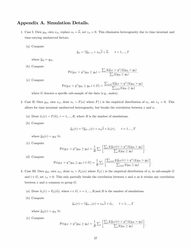
Appendix A. Simulation Details.

1. Case I. Own 0, own , replace = b, set = 0. This eliminates heterogeneity due to time invariant andtime-varying unobserved factors.

(a) Compute b = bb−1 + b + b = 1

where b0 = 0.

(b) Compute

Pr( ∗|0 ≥ 0) =

P I(b ∗) I(0 0)P

I(0 ≥ 0)

(c) Compute

Pr( ∗|0 ≥ 0 ∈ ) =

P∈ I(b ∗) I(0 0)P

∈ I(0 ≥ 0)

where denotes a specific sub-sample of the data (e.g., males).

2. Case II. Own 0, own , draw ∼ () where (·) is the empirical distribution of , set = 0. This

allows for time invariant unobserved heterogeneity, but breaks the correlation between and .

(a) Draw e() ∼ (b), = 1 , where is the number of simulations.

(b) Compute b() = bb−1() + b + e() = 1

where b0() = 0 ∀.

(c) Compute

Pr( ∗|0 ≥ 0) =1

P

∙P I(b () ∗) I(0 0)P

I(0 ≥ 0)

¸

(d) Compute

Pr( ∗|0 ≥ 0 ∈ ) =1

P

∙P∈ I(b () ∗) I(0 0)P

∈ I(0 ≥ 0)

¸

3. Case III. Own 0, own , draw ∼ () where (·) is the empirical distribution of in sub-sample and ∈ , set = 0. This only partially breaks the correlation between and as it retains any correlation

between and common to group .

(a) Draw e() ∼ (b), where ∈ , = 1 and is the number of simulations.

(b) Compute b() = bb−1() + b + e = 1

where b0() = 0 ∀.

(c) Compute

Pr( ∗|0 ≥ 0) =1

P

∙P I(b () ∗) I(0 0)P

I(0 ≥ 0)

¸

27

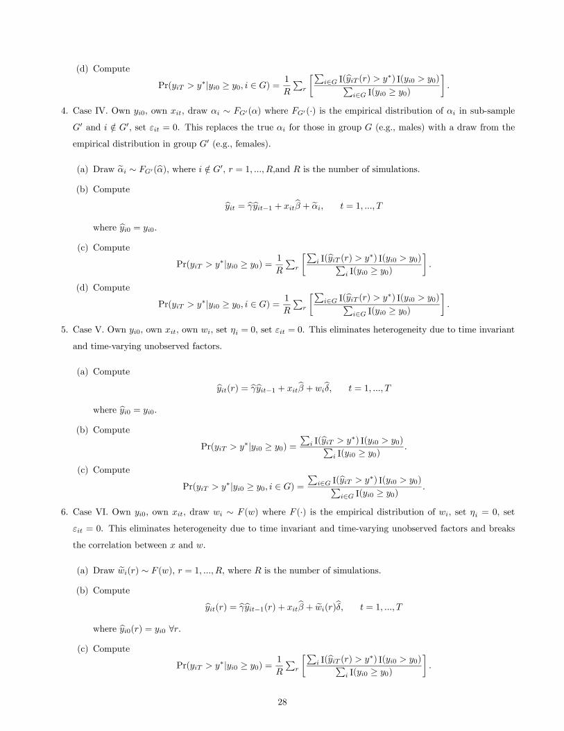
(d) Compute

Pr( ∗|0 ≥ 0 ∈ ) =1

P

∙P∈ I(b () ∗) I(0 0)P

∈ I(0 ≥ 0)

¸

4. Case IV. Own 0, own , draw ∼ 0() where 0(·) is the empirical distribution of in sub-sample0 and ∈ 0, set = 0. This replaces the true for those in group (e.g., males) with a draw from the

empirical distribution in group 0 (e.g., females).

(a) Draw e ∼ 0(b), where ∈ 0, = 1 and is the number of simulations.

(b) Compute b = bb−1 + b + e = 1

where b0 = 0.

(c) Compute

Pr( ∗|0 ≥ 0) =1

P

∙P I(b () ∗) I(0 0)P

I(0 ≥ 0)

¸

(d) Compute

Pr( ∗|0 ≥ 0 ∈ ) =1

P

∙P∈ I(b () ∗) I(0 0)P

∈ I(0 ≥ 0)

¸

5. Case V. Own 0, own , own , set = 0, set = 0. This eliminates heterogeneity due to time invariant

and time-varying unobserved factors.

(a) Compute b() = bb−1 + b + b = 1

where b0 = 0.

(b) Compute

Pr( ∗|0 ≥ 0) =

P I(b ∗) I(0 0)P

I(0 ≥ 0)

(c) Compute

Pr( ∗|0 ≥ 0 ∈ ) =

P∈ I(b ∗) I(0 0)P

∈ I(0 ≥ 0)

6. Case VI. Own 0, own , draw ∼ () where (·) is the empirical distribution of , set = 0, set

= 0. This eliminates heterogeneity due to time invariant and time-varying unobserved factors and breaks

the correlation between and .

(a) Draw e() ∼ (), = 1 , where is the number of simulations.

(b) Compute b() = bb−1() + b + e()b = 1

where b0() = 0 ∀.

(c) Compute

Pr( ∗|0 ≥ 0) =1

P

∙P I(b () ∗) I(0 0)P

I(0 ≥ 0)

¸

28

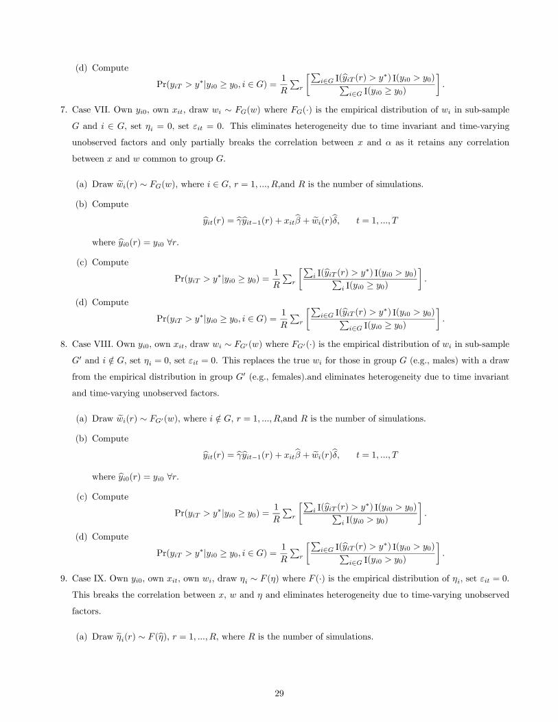
(d) Compute

Pr( ∗|0 ≥ 0 ∈ ) =1

P

∙P∈ I(b () ∗) I(0 0)P

∈ I(0 ≥ 0)

¸

7. Case VII. Own 0, own , draw ∼ () where (·) is the empirical distribution of in sub-sample

and ∈ , set = 0, set = 0. This eliminates heterogeneity due to time invariant and time-varying

unobserved factors and only partially breaks the correlation between and as it retains any correlation

between and common to group .

(a) Draw e() ∼ (), where ∈ , = 1 and is the number of simulations.

(b) Compute b() = bb−1() + b + e()b = 1

where b0() = 0 ∀.

(c) Compute

Pr( ∗|0 ≥ 0) =1

P

∙P I(b () ∗) I(0 0)P

I(0 ≥ 0)

¸

(d) Compute

Pr( ∗|0 ≥ 0 ∈ ) =1

P

∙P∈ I(b () ∗) I(0 0)P

∈ I(0 ≥ 0)

¸

8. Case VIII. Own 0, own , draw ∼ 0() where 0(·) is the empirical distribution of in sub-sample

0 and ∈ , set = 0, set = 0. This replaces the true for those in group (e.g., males) with a draw

from the empirical distribution in group 0 (e.g., females).and eliminates heterogeneity due to time invariant

and time-varying unobserved factors.

(a) Draw e() ∼ 0(), where ∈ , = 1 and is the number of simulations.

(b) Compute b() = bb−1() + b + e()b = 1

where b0() = 0 ∀.

(c) Compute

Pr( ∗|0 ≥ 0) =1

P

∙P I(b () ∗) I(0 0)P

I(0 0)

¸

(d) Compute

Pr( ∗|0 ≥ 0 ∈ ) =1

P

∙P∈ I(b () ∗) I(0 0)P

∈ I(0 0)

¸

9. Case IX. Own 0, own , own , draw ∼ () where (·) is the empirical distribution of , set = 0.This breaks the correlation between , and and eliminates heterogeneity due to time-varying unobserved

factors.

(a) Draw e() ∼ (b), = 1 , where is the number of simulations.

29

(b) Compute b() = bb−1() + b + b + e() = 1

where b0() = 0 ∀.

(c) Compute

Pr( ∗|0 ≥ 0) =1

P

∙P I(b () ∗) I(0 0)P

I(0 ≥ 0)

¸

(d) Compute

Pr( ∗|0 ≥ 0 ∈ ) =1

P

∙P∈ I(b () ∗) I(0 0)P

∈ I(0 ≥ 0)

¸

10. Case X. Own 0, own , own , draw ∼ () where (·) is the empirical distribution of in sub-sample and ∈ , set = 0. This only partially breaks the correlation between , and as it retains

any correlation between , and common to group and eliminates heterogeneity due to time invariant

and time-varying unobserved factors.

(a) Draw e() ∼ (b), where ∈ , = 1 and is the number of simulations.

(b) Compute b() = bb−1() + b + b + e() = 1

where b0() = 0 ∀.

(c) Compute

Pr( ∗|0 ≥ 0) =1

P

∙P I(b () ∗) I(0 0)P

I(0 ≥ 0)

¸

(d) Compute

Pr( ∗|0 ≥ 0 ∈ ) =1

P

∙P∈ I(b () ∗) I(0 0)P

∈ I(0 ≥ 0)

¸

11. Case XI. Own 0, own , own , draw ∼ 0() where 0(·) is the empirical distribution of insub-sample 0 and ∈ , set = 0. This replaces the true for those in group (e.g., males) with a draw

from the empirical distribution in group 0 (e.g., females) and eliminates heterogeneity due to time invariant

and time-varying unobserved factors.

(a) Draw e() ∼ 0(b), where ∈ , = 1 and is the number of simulations.

(b) Compute b() = bb−1() + b + b + e() = 1

where b0() = 0 ∀.

(c) Compute

Pr( ∗|0 ≥ 0) =1

P

∙P I(b () ∗) I(0 0)P

I(0 0)

¸

(d) Compute

Pr( ∗|0 ≥ 0 ∈ ) =1

P

∙P∈ I(b () ∗) I(0 0)P

∈ I(0 0)

¸

30

12. Case XII. Own 0, replace = , own , set = 0. The eliminates heterogeneity due to time-varying

factors.

(a) Compute b = bb−1 + b + b = 1

where b0 = 0.

(b) Compute

Pr( ∗|0 ≥ 0) =

P I(b ∗) I(0 0)P

I(0 ≥ 0)

(c) Compute

Pr( ∗|0 ≥ 0 ∈ ) =

P∈ I(b ∗) I(0 0)P

∈ I(0 ≥ 0)

where denotes a specific sub-sample of the data (e.g., males).

13. Case XIII. Own 0, draw · ∼ (1 ) where (·) is the empirical joint distribution of 1 , own, set = 0. This breaks the correlation between and and eliminates heterogeneity due to time-varying

unobserved factors.

(a) Draw e·() ∼ (1 ), = 1 , where is the number of simulations.

(b) Compute b() = bb−1() + e()b + = 1

where b0() = 0 ∀.

(c) Compute

Pr( ∗|0 ≥ 0) =1

P

∙P I(b () ∗) I(0 0)P

I(0 ≥ 0)

¸

(d) Compute

Pr( ∗|0 ≥ 0 ∈ ) =1

P

∙P∈ I(b () ∗) I(0 0)P

∈ I(0 ≥ 0)

¸

14. Case XIV. Own 0, draw · ∼ (1 ) where (·) is the empirical joint distribution of 1 insub-sample and ∈ , own , set = 0. This only partially breaks the correlation between and as it

retains any correlation between and common to group and eliminates heterogeneity due to time-varying

unobserved factors.

(a) Draw e·() ∼ (1 ), where ∈ , = 1 , where is the number of simulations.

(b) Compute b() = bb−1() + e()b + = 1

where b0() = 0 ∀.

(c) Compute

Pr( ∗|0 ≥ 0) =1

P

∙P I(b () ∗) I(0 0)P

I(0 0)

¸

31

(d) Compute

Pr( ∗|0 ≥ 0 ∈ ) =1

P

∙P∈ I(b () ∗) I(0 0)P

∈ I(0 0)

¸

15. Case XV. Own 0, draw · ∼ (1 ) where (·) is the empirical joint distribution of 1 insub-sample and ∈ , own , set = 0. This replaces the true · for those in group (e.g., males)

with a draw from the empirical distribution in group 0 (e.g., females) and eliminates heterogeneity due to

time-varying unobserved factors.

(a) Draw e·() ∼ 0(1 ), where ∈ 0, = 1 , where is the number of simulations.

(b) Compute b() = bb−1() + e()b + = 1

where b0() = 0 ∀.

(c) Compute

Pr( ∗|0 ≥ 0) =1

P

∙P I(b () ∗) I(0 0)P

I(0 0)

¸

(d) Compute

Pr( ∗|0 ≥ 0 ∈ ) =1

P

∙P∈ I(b () ∗) I(0 0)P

∈ I(0 0)

¸

16. Case XVI. Own 0, own , own , draw · ∼ (1 ) where (·) is the empirical distribution of ·.This breaks the correlation between and .

(a) Draw e·() ∼ (b1 b ), = 1 , where is the number of simulations.

(b) Compute b() = bb−1() + b + b + e() = 1

where b0() = 0 ∀.

(c) Compute

Pr( ∗|0 ≥ 0) =1

P

∙P I(b () ∗) I(0 0)P

I(0 ≥ 0)

¸

(d) Compute

Pr( ∗|0 ≥ 0 ∈ ) =1

P

∙P∈ I(b () ∗) I(0 0)P

∈ I(0 ≥ 0)

¸

17. Case XVII. Own 0, own , own , draw · ∼ (1 ) where (·) is the empirical distribution of· in sub-sample and ∈ . This only partially breaks the correlation between and as it retains any

correlation between and common to group .

(a) Draw e·() ∼ (b1 b ), where ∈ , = 1 and is the number of simulations.

(b) Compute b() = bb−1() + b + b + e() = 1

where b0() = 0 ∀.

32

(c) Compute

Pr( ∗|0 ≥ 0) =1

P

∙P I(b () ∗) I(0 0)P

I(0 0)

¸

(d) Compute

Pr( ∗|0 ≥ 0 ∈ ) =1

P

∙P∈ I(b () ∗) I(0 0)P

∈ I(0 0)

¸

18. Case XVIII. Own 0, own , own , draw · ∼ 0(1 ) where 0(·) is the empirical distribution of· in sub-sample 0 and ∈ . This replaces the true · for those in group (e.g., males) with a draw from

the empirical distribution in group 0 (e.g., females).

(a) Draw e·() ∼ 0(b1 b ), where ∈ , = 1 and is the number of simulations.

(b) Compute b() = bb−1() + b + b + e() = 1

where b0() = 0 ∀.

(c) Compute

Pr( ∗|0 ≥ 0) =1

P

∙P I(b () ∗) I(0 0)P

I(0 ≥ 0)

¸

(d) Compute

Pr( ∗|0 ≥ 0 ∈ ) =1

P

∙P∈ I(b () ∗) I(0 0)P

∈ I(0 ≥ 0)

¸

19. Case XIX. Own 0, own , draw · · ∼ (1 1 ) where (·) is the empirical joint distributionof 1 1 . This breaks the correlation between and , .

(a) Draw e·()e·() ∼ (1 b1 b ), = 1 , where is the number of simulations.

(b) Compute b() = bb−1() + e()b + b + e() = 1

where b0() = 0 ∀.

(c) Compute

Pr( ∗|0 ≥ 0) =1

P

∙P I(b () ∗) I(0 0)P

I(0 ≥ 0)

¸

(d) Compute

Pr( ∗|0 ≥ 0 ∈ ) =1

P

∙P∈ I(b () ∗) I(0 0)P

∈ I(0 ≥ 0)

¸

20. Case XX. Own 0,own , draw · · ∼ (1 1 ) where (·) is the empirical joint distributionof 1 1 in sub-sample and ∈ . This only partially breaks the correlation between and ,

as it retains any correlation between and , common to group .

(a) Draw e·()e·() ∼ (1 b1 b ), where ∈ , = 1 and is the number of simulations.

(b) Compute b() = bb−1() + e()b + b + e() = 1

where b0() = 0 ∀.

33

(c) Compute

Pr( ∗|0 ≥ 0) =1

P

∙P I(b () ∗) I(0 0)P

I(0 0)

¸

(d) Compute

Pr( ∗|0 ≥ 0 ∈ ) =1

P

∙P∈ I(b () ∗) I(0 0)P

∈ I(0 0)

¸

21. Case XXI. Own 0, own , draw · · ∼ (1 1 ) where 0(·) is the empirical joint distributionof 1 1 in sub-sample

0 and ∈ . This replaces the true · and · for those in group (e.g.,

males) with a draw from the empirical distribution in group 0 (e.g., females).

(a) Draw e·()e·() ∼ 0(1 b1 b ), where ∈ , = 1 and is the number of simulations.

(b) Compute b() = bb−1() + e()b + b + e() = 1

where b0() = 0 ∀.

(c) Compute

Pr( ∗|0 ≥ 0) =1

P

∙P I(b () ∗) I(0 0)P

I(0 ≥ 0)

¸

(d) Compute

Pr( ∗|0 ≥ 0 ∈ ) =1

P

∙P∈ I(b () ∗) I(0 0)P

∈ I(0 ≥ 0)

¸

34

Appendix B. Figures.

35

Figure B1. Weight: Decomposition. Notes: Data from ECLS-K. Empirical distributions of the outcome, yit, and the various estimated components of the dynamic model yit = γyit-1 + Xitβ + αi + εit. Data from ECLS-K. See text for further details.

0.1

.2.3

.4

-4 -2 0 2 4Weight Z-Scores

White Non-White0

510

15

-.2 -.1 0 .1 .2Xb

White Non-White

0.5

11.

5

-1 -.5 0 .5 1Fixed Effects

White Non-White

0.5

11.

5

-2 -1 0 1 2Idiosyncratic Errors

White Non-White

0.1

.2.3

.4

-4 -2 0 2 4Weight Z-Scores

Male Female

02

46

810

-.2 -.1 0 .1 .2Xb

Male Female

0.5

11.

5

-1 -.5 0 .5 1Fixed Effects

Male Female

0.5

11.

5

-2 -1 0 1 2Idiosyncratic Errors

Male Female

0.1

.2.3

.4

-4 -2 0 2 4Weight Z-Scores

Urban Non-Urban

02

46

810

-.2 -.1 0 .1 .2Xb

Urban Non-Urban

0.5

11.

5

-1 -.5 0 .5 1Fixed Effects

Urban Non-Urban

0.5

11.

5

-2 -1 0 1 2Idiosyncratic Errors

Urban Non-Urban

0.1

.2.3

.4

-4 -2 0 2 4Weight Z-Scores

College Non-College

05

1015

-.2 -.1 0 .1 .2Xb

College Non-College

0.5

11.

5

-1 -.5 0 .5 1Fixed Effects

College Non-College

0.5

11.

5

-2 -1 0 1 2Idiosyncratic Errors

College Non-College

0.1

.2.3

.4

-4 -2 0 2 4Weight Z-Scores

Low SES High SES

05

1015

-.2 -.1 0 .1 .2Xb

Low SES High SES

0.5

11.

5

-1 -.5 0 .5 1Fixed Effects

Low SES High SES

0.5

11.

5

-2 -1 0 1 2Idiosyncratic Errors

Low SES High SES

Figure B2. Weight: Decomposition of Fixed Effects. Notes: Data from ECLS-K. Empirical distributions of the estimated fixed effects, αit, and its components obtained from the dynamic model yit = γyit-1 + Xitβ + αi + εit, where αi = wiδ + ηi. See text for further details.

0.5

11.

5

-1 -.5 0 .5 1Fixed Effects

White Non-White

02

46

8

0 .1 .2 .3 .4 .5Observed

White Non-White

0.5

11.

5

-1 -.5 0 .5 1Unobserved

White Non-White

0.5

11.

5

-1 -.5 0 .5 1Fixed Effects

Male Female

02

46

8

0 .1 .2 .3 .4 .5Observed

Male Female

0.5

11.

5

-1 -.5 0 .5 1Unobserved

Male Female

0.5

11.

5

-1 -.5 0 .5 1Fixed Effects

Urban Non-Urban

02

46

8

0 .1 .2 .3 .4 .5Observed

Urban Non-Urban

0.5

11.

5

-1 -.5 0 .5 1Unobserved

Urban Non-Urban

0.5

11.

5

-1 -.5 0 .5 1Fixed Effects

College Non-College

02

46

8

0 .1 .2 .3 .4 .5Observed

College Non-College

0.5

11.

5

-1 -.5 0 .5 1Unobserved

College Non-College

0.5

11.

5

-1 -.5 0 .5 1Fixed Effects

Low SES High SES

02

46

8

0 .1 .2 .3 .4 .5Observed

Low SES High SES

0.5

11.

5

-1 -.5 0 .5 1Unobserved

Low SES High SES

Figure B3. Height: Decomposition. Notes: See Figure B1 and text for details.

0.1

.2.3

.4

-4 -2 0 2 4Height Z-Scores

White Non-White0

24

68

-.4 -.2 0 .2 .4Xb

White Non-White

0.2

.4.6

.81

-1 -.5 0 .5 1Fixed Effects

White Non-White

0.5

11.

5

-2 -1 0 1 2Idiosyncratic Errors

White Non-White

0.1

.2.3

.4

-4 -2 0 2 4Height Z-Scores

Male Female

02

46

8

-.4 -.2 0 .2 .4Xb

Male Female0

.2.4

.6.8

1

-1 -.5 0 .5 1Fixed Effects

Male Female

0.5

11.

5

-2 -1 0 1 2Idiosyncratic Errors

Male Female

0.1

.2.3

.4

-4 -2 0 2 4Height Z-Scores

Urban Non-Urban

02

46

8

-.4 -.2 0 .2 .4Xb

Urban Non-Urban

0.2

.4.6

.81

-1 -.5 0 .5 1Fixed Effects

Urban Non-Urban

0.5

11.

5

-2 -1 0 1 2Idiosyncratic Errors

Urban Non-Urban

0.1

.2.3

.4

-4 -2 0 2 4Height Z-Scores

College Non-College

02

46

8

-.4 -.2 0 .2 .4Xb

College Non-College

0.2

.4.6

.81

-1 -.5 0 .5 1Fixed Effects

College Non-College

0.5

11.

5

-2 -1 0 1 2Idiosyncratic Errors

College Non-College

0.1

.2.3

.4

-4 -2 0 2 4Height Z-Scores

Low SES High SES

02

46

8

-.4 -.2 0 .2 .4Xb

Low SES High SES

0.2

.4.6

.81

-1 -.5 0 .5 1Fixed Effects

Low SES High SES

0.5

11.

5

-2 -1 0 1 2Idiosyncratic Errors

Low SES High SES

Figure B4. Height: Decomposition of Fixed Effects. Notes: See Figure B2 and text for details.

0.2

.4.6

.81

-1 -.5 0 .5 1Fixed Effects

White Non-White

02

46

-.5 0 .5Observed

White Non-White

0.2

.4.6

.81

-1 -.5 0 .5 1Unobserved

White Non-White

0.2

.4.6

.81

-1 -.5 0 .5 1Fixed Effects

Male Female

01

23

45

-.5 0 .5Observed

Male Female

0.2

.4.6

.81

-1 -.5 0 .5 1Unobserved

Male Female

0.2

.4.6

.81

-1 -.5 0 .5 1Fixed Effects

Urban Non-Urban

01

23

45

-.5 0 .5Observed

Urban Non-Urban

0.2

.4.6

.81

-1 -.5 0 .5 1Unobserved

Urban Non-Urban

0.2

.4.6

.81

-1 -.5 0 .5 1Fixed Effects

College Non-College

01

23

45

-.5 0 .5Observed

College Non-College

0.2

.4.6

.81

-1 -.5 0 .5 1Unobserved

College Non-College

0.2

.4.6

.81

-1 -.5 0 .5 1Fixed Effects

Low SES High SES

01

23

45

-.5 0 .5Observed

Low SES High SES

0.2

.4.6

.81

-1 -.5 0 .5 1Unobserved

Low SES High SES

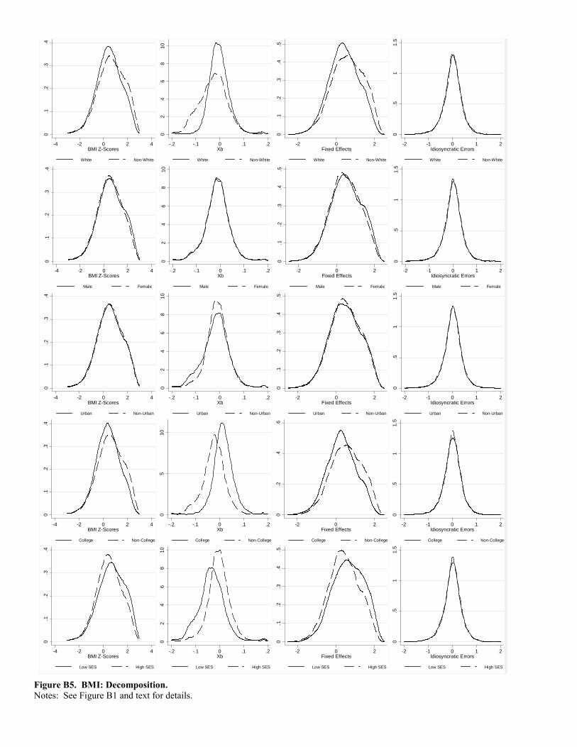
Figure B5. BMI: Decomposition. Notes: See Figure B1 and text for details.

0.1

.2.3

.4

-4 -2 0 2 4BMI Z-Scores

White Non-White0

24

68

10

-.2 -.1 0 .1 .2Xb

White Non-White

0.1

.2.3

.4.5

-2 0 2Fixed Effects

White Non-White

0.5

11.

5

-2 -1 0 1 2Idiosyncratic Errors

White Non-White

0.1

.2.3

.4

-4 -2 0 2 4BMI Z-Scores

Male Female

02

46

810

-.2 -.1 0 .1 .2Xb

Male Female0

.1.2

.3.4

.5

-2 0 2Fixed Effects

Male Female

0.5

11.

5

-2 -1 0 1 2Idiosyncratic Errors

Male Female

0.1

.2.3

.4

-4 -2 0 2 4BMI Z-Scores

Urban Non-Urban

02

46

810

-.2 -.1 0 .1 .2Xb

Urban Non-Urban

0.1

.2.3

.4.5

-2 0 2Fixed Effects

Urban Non-Urban

0.5

11.

5

-2 -1 0 1 2Idiosyncratic Errors

Urban Non-Urban

0.1

.2.3

.4

-4 -2 0 2 4BMI Z-Scores

College Non-College

05

10

-.2 -.1 0 .1 .2Xb

College Non-College

0.2

.4.6

-2 0 2Fixed Effects

College Non-College

0.5

11.

5

-2 -1 0 1 2Idiosyncratic Errors

College Non-College

0.1

.2.3

.4

-4 -2 0 2 4BMI Z-Scores

Low SES High SES

02

46

810

-.2 -.1 0 .1 .2Xb

Low SES High SES

0.1

.2.3

.4.5

-2 0 2Fixed Effects

Low SES High SES

0.5

11.

5

-2 -1 0 1 2Idiosyncratic Errors

Low SES High SES

Figure B6. BMI: Decomposition of Fixed Effects. Notes: See Figure B2 and text for details.

0.1

.2.3

.4.5

-2 0 2Fixed Effects

White Non-White

0.5

11.

52

2.5

0 .5 1 1.5Observed

White Non-White

0.2

.4.6

-2 0 2Unobserved

White Non-White

0.1

.2.3

.4.5

-2 0 2Fixed Effects

Male Female

0.5

11.

52

0 .5 1 1.5Observed

Male Female

0.1

.2.3

.4.5

-2 0 2Unobserved

Male Female

0.1

.2.3

.4.5

-2 0 2Fixed Effects

Urban Non-Urban

0.5

11.

52

0 .5 1 1.5Observed

Urban Non-Urban

0.1

.2.3

.4.5

-2 0 2Unobserved

Urban Non-Urban

0.2

.4.6

-2 0 2Fixed Effects

College Non-College

01

23

0 .5 1 1.5Observed

College Non-College

0.2

.4.6

-2 0 2Unobserved

College Non-College

0.1

.2.3

.4.5

-2 0 2Fixed Effects

Low SES High SES

0.5

11.

52

2.5

0 .5 1 1.5Observed

Low SES High SES

0.1

.2.3

.4.5

-2 0 2Unobserved

Low SES High SES

Figure B7. Weight: Decomposition. Notes: Data from ECLS-B. Empirical distributions of the outcome, yit, and the various estimated components of the dynamic model yit = γyit-1 + Xitβ + αi + εit. See text for further details.

0.1

.2.3

.4

-4 -2 0 2 4Weight Z-Scores

White Non-White0

.51

1.5

2

-.5 0 .5 1 1.5 2Xb

White Non-White

0.1

.2.3

.4.5

-4 -2 0 2 4Fixed Effects

White Non-White

0.5

1

-2 -1 0 1 2Idiosyncratic Errors

White Non-White

0.1

.2.3

.4

-4 -2 0 2 4Weight Z-Scores

Male Female

0.5

11.

5

-.5 0 .5 1 1.5 2Xb

Male Female0

.1.2

.3.4

.5

-4 -2 0 2 4Fixed Effects

Male Female

0.2

.4.6

.81

-2 -1 0 1 2Idiosyncratic Errors

Male Female

0.1

.2.3

.4

-4 -2 0 2 4Weight Z-Scores

Urban Non-Urban

0.5

11.

5

-.5 0 .5 1 1.5 2Xb

Urban Non-Urban

0.1

.2.3

.4.5

-4 -2 0 2 4Fixed Effects

Urban Non-Urban

0.2

.4.6

.81

-2 -1 0 1 2

Idiosyncratic Errors

Urban Non-Urban

0.1

.2.3

.4

-4 -2 0 2 4Weight Z-Scores

College Non-College

0.5

11.

5

-.5 0 .5 1 1.5 2Xb

College Non-College

0.1

.2.3

.4.5

-4 -2 0 2 4Fixed Effects

College Non-College

0.5

11.

5

-2 -1 0 1 2Idiosyncratic Errors

College Non-College

0.1

.2.3

.4

-4 -2 0 2 4Weight Z-Scores

Low SES High SES

0.5

11.

5

-.5 0 .5 1 1.5 2Xb

Low SES High SES

0.1

.2.3

.4.5

-4 -2 0 2 4Fixed Effects

Low SES High SES

0.5

1

-2 -1 0 1 2Idiosyncratic Errors

Low SES High SES

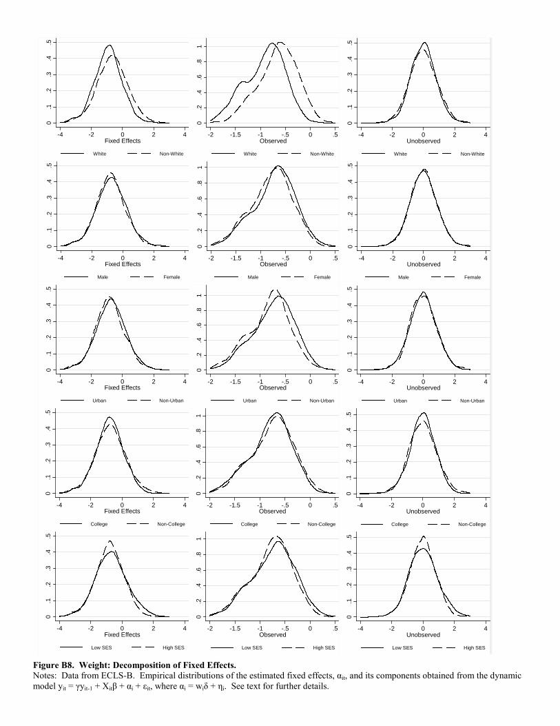
Figure B8. Weight: Decomposition of Fixed Effects. Notes: Data from ECLS-B. Empirical distributions of the estimated fixed effects, αit, and its components obtained from the dynamic model yit = γyit-1 + Xitβ + αi + εit, where αi = wiδ + ηi. See text for further details.

0.1

.2.3

.4.5

-4 -2 0 2 4Fixed Effects

White Non-White

0.2

.4.6

.81

-2 -1.5 -1 -.5 0 .5Observed

White Non-White

0.1

.2.3

.4.5

-4 -2 0 2 4Unobserved

White Non-White

0.1

.2.3

.4.5

-4 -2 0 2 4Fixed Effects

Male Female

0.2

.4.6

.81

-2 -1.5 -1 -.5 0 .5Observed

Male Female

0.1

.2.3

.4.5

-4 -2 0 2 4Unobserved

Male Female

0.1

.2.3

.4.5

-4 -2 0 2 4Fixed Effects

Urban Non-Urban

0.2

.4.6

.81

-2 -1.5 -1 -.5 0 .5Observed

Urban Non-Urban

0.1

.2.3

.4.5

-4 -2 0 2 4Unobserved

Urban Non-Urban

0.1

.2.3

.4.5

-4 -2 0 2 4Fixed Effects

College Non-College

0.2

.4.6

.81

-2 -1.5 -1 -.5 0 .5Observed

College Non-College

0.1

.2.3

.4.5

-4 -2 0 2 4Unobserved

College Non-College

0.1

.2.3

.4.5

-4 -2 0 2 4Fixed Effects

Low SES High SES

0.2

.4.6

.81

-2 -1.5 -1 -.5 0 .5Observed

Low SES High SES

0.1

.2.3

.4.5

-4 -2 0 2 4Unobserved

Low SES High SES

Figure B9. Height: Decomposition. Notes: See Figure B7 and text for details.

0.0

1.0

2.0

3

40 60 80 100 120 140Height (cms)

White Non-White0

.01

.02

.03

.04

0 10 20 30 40 50Xb

White Non-White

0.0

2.0

4.0

6.0

8.1

60 70 80 90Fixed Effects

White Non-White

.1.1

5.2

.25

.3

-2 -1 0 1 2Idiosyncratic Errors

White Non-White

0.0

1.0

2.0

3

40 60 80 100 120 140Height (cms)

Male Female

0.0

1.0

2.0

3.0

4

0 10 20 30 40 50Xb

Male Female

0.0

2.0

4.0

6.0

8.1

60 70 80 90

Fixed Effects

Male Female

.1.1

5.2

.25

.3

-2 -1 0 1 2Idiosyncratic Errors

Male Female

0.0

1.0

2.0

3

40 60 80 100 120 140Height (cms)

Urban Non-Urban

0.0

1.0

2.0

3.0

4

0 10 20 30 40 50Xb

Urban Non-Urban

0.0

2.0

4.0

6.0

8.1

60 70 80 90Fixed Effects

Urban Non-Urban

.1.1

5.2

.25

.3

-2 -1 0 1 2Idiosyncratic Errors

Urban Non-Urban

0.0

1.0

2.0

3

40 60 80 100 120 140Height (cms)

College Non-College

0.0

1.0

2.0

3.0

4

0 10 20 30 40 50Xb

College Non-College

0.0

2.0

4.0

6.0

8.1

60 70 80 90Fixed Effects

College Non-College

.1.1

5.2

.25

.3

-2 -1 0 1 2Idiosyncratic Errors

College Non-College

0.0

1.0

2.0

3

40 60 80 100 120 140Height (cms)

Low SES High SES

0.0

1.0

2.0

3.0

4

0 10 20 30 40 50Xb

Low SES High SES

0.0

2.0

4.0

6.0

8.1

60 70 80 90Fixed Effects

Low SES High SES

.1.1

5.2

.25

.3

-2 -1 0 1 2Idiosyncratic Errors

Low SES High SES

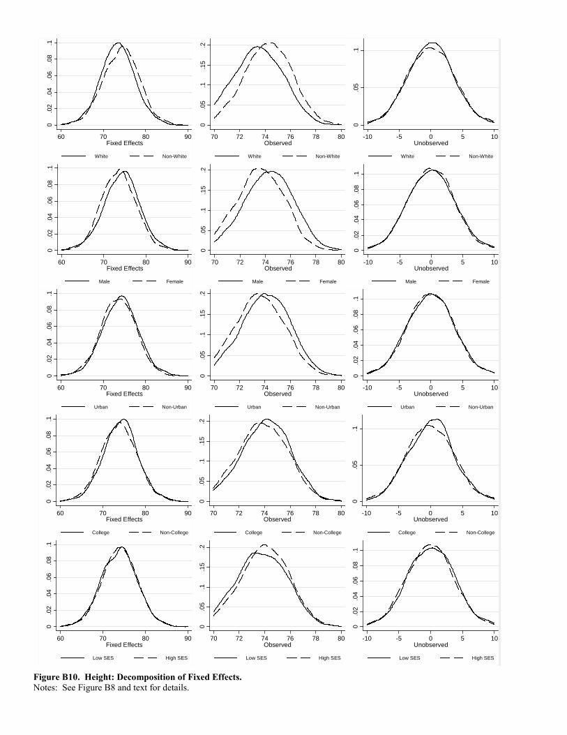
Figure B10. Height: Decomposition of Fixed Effects. Notes: See Figure B8 and text for details.

0.0

2.0

4.0

6.0

8.1

60 70 80 90Fixed Effects

White Non-White

0.0

5.1

.15

.2

70 72 74 76 78 80Observed

White Non-White

0.0

5.1

-10 -5 0 5 10Unobserved

White Non-White

0.0

2.0

4.0

6.0

8.1

60 70 80 90Fixed Effects

Male Female

0.0

5.1

.15

.2

70 72 74 76 78 80Observed

Male Female

0.0

2.0

4.0

6.0

8.1

-10 -5 0 5 10Unobserved

Male Female

0.0

2.0

4.0

6.0

8.1

60 70 80 90Fixed Effects

Urban Non-Urban

0.0

5.1

.15

.2

70 72 74 76 78 80Observed

Urban Non-Urban

0.0

2.0

4.0

6.0

8.1

-10 -5 0 5 10Unobserved

Urban Non-Urban

0.0

2.0

4.0

6.0

8.1

60 70 80 90Fixed Effects

College Non-College

0.0

5.1

.15

.2

70 72 74 76 78 80Observed

College Non-College

0.0

5.1

-10 -5 0 5 10Unobserved

College Non-College

0.0

2.0

4.0

6.0

8.1

60 70 80 90Fixed Effects

Low SES High SES

0.0

5.1

.15

.2

70 72 74 76 78 80Observed

Low SES High SES

0.0

2.0

4.0

6.0

8.1

-10 -5 0 5 10Unobserved

Low SES High SES

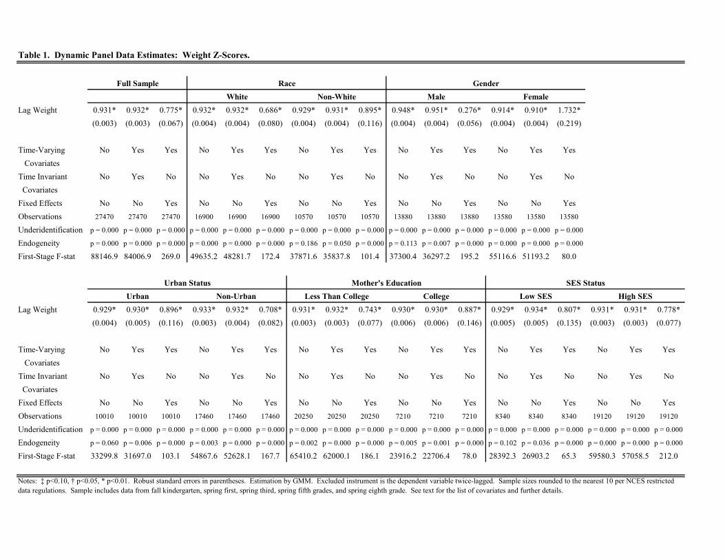
Table 1. Dynamic Panel Data Estimates: Weight Z-Scores.

Lag Weight 0.931* 0.932* 0.775* 0.932* 0.932* 0.686* 0.929* 0.931* 0.895* 0.948* 0.951* 0.276* 0.914* 0.910* 1.732*(0.003) (0.003) (0.067) (0.004) (0.004) (0.080) (0.004) (0.004) (0.116) (0.004) (0.004) (0.056) (0.004) (0.004) (0.219)

Time-Varying No Yes Yes No Yes Yes No Yes Yes No Yes Yes No Yes Yes CovariatesTime Invariant No Yes No No Yes No No Yes No No Yes No No Yes No CovariatesFixed Effects No No Yes No No Yes No No Yes No No Yes No No YesObservations 27470 27470 27470 16900 16900 16900 10570 10570 10570 13880 13880 13880 13580 13580 13580

Underidentification p = 0.000 p = 0.000 p = 0.000 p = 0.000 p = 0.000 p = 0.000 p = 0.000 p = 0.000 p = 0.000 p = 0.000 p = 0.000 p = 0.000 p = 0.000 p = 0.000 p = 0.000

Endogeneity p = 0.000 p = 0.000 p = 0.000 p = 0.000 p = 0.000 p = 0.000 p = 0.186 p = 0.050 p = 0.000 p = 0.113 p = 0.007 p = 0.000 p = 0.000 p = 0.000 p = 0.000

First-Stage F-stat 88146.9 84006.9 269.0 49635.2 48281.7 172.4 37871.6 35837.8 101.4 37300.4 36297.2 195.2 55116.6 51193.2 80.0

Lag Weight 0.929* 0.930* 0.896* 0.933* 0.932* 0.708* 0.931* 0.932* 0.743* 0.930* 0.930* 0.887* 0.929* 0.934* 0.807* 0.931* 0.931* 0.778*(0.004) (0.005) (0.116) (0.003) (0.004) (0.082) (0.003) (0.003) (0.077) (0.006) (0.006) (0.146) (0.005) (0.005) (0.135) (0.003) (0.003) (0.077)

Time-Varying No Yes Yes No Yes Yes No Yes Yes No Yes Yes No Yes Yes No Yes Yes CovariatesTime Invariant No Yes No No Yes No No Yes No No Yes No No Yes No No Yes No CovariatesFixed Effects No No Yes No No Yes No No Yes No No Yes No No Yes No No YesObservations 10010 10010 10010 17460 17460 17460 20250 20250 20250 7210 7210 7210 8340 8340 8340 19120 19120 19120

Underidentification p = 0.000 p = 0.000 p = 0.000 p = 0.000 p = 0.000 p = 0.000 p = 0.000 p = 0.000 p = 0.000 p = 0.000 p = 0.000 p = 0.000 p = 0.000 p = 0.000 p = 0.000 p = 0.000 p = 0.000 p = 0.000

Endogeneity p = 0.060 p = 0.006 p = 0.000 p = 0.003 p = 0.000 p = 0.000 p = 0.002 p = 0.000 p = 0.000 p = 0.005 p = 0.001 p = 0.000 p = 0.102 p = 0.036 p = 0.000 p = 0.000 p = 0.000 p = 0.000

First-Stage F-stat 33299.8 31697.0 103.1 54867.6 52628.1 167.7 65410.2 62000.1 186.1 23916.2 22706.4 78.0 28392.3 26903.2 65.3 59580.3 57058.5 212.0

Notes: ‡ p<0.10, † p<0.05, * p<0.01. Robust standard errors in parentheses. Estimation by GMM. Excluded instrument is the dependent variable twice-lagged. Sample sizes rounded to the nearest 10 per NCES restricted data regulations. Sample includes data from fall kindergarten, spring first, spring third, spring fifth grades, and spring eighth grade. See text for the list of covariates and further details.

Urban Non-Urban Less Than College College Low SES High SES

Full Sample Race Gender

Urban Status Mother's Education SES Status

White Non-White Male Female

Table 2. Dynamic Simulations: Weight Z-Scores, Pr(yiT≥85th percentile | yi1≥85th percentile).

Full

Sample White Non-White Male Female Urban Non-Urban Non-College College Low SES High SES

Benchmark 0.840 0.823 0.861 0.846 0.833 0.840 0.840 0.870 0.748 0.880 0.820

Panel I. Own Xs, ε=0, and α=E[α] 0.753 0.681 0.846 0.765 0.739 0.776 0.740 0.800 0.609 0.868 0.695

α~f(α) 0.576 0.555 0.604 0.581 0.570 0.586 0.570 0.588 0.540 0.609 0.559

α~fi(α) 0.552 0.608 0.597 0.555 0.565 0.584 0.607 0.484 0.637 0.547

α~f-i(α) 0.562 0.602 0.567 0.586 0.599 0.551 0.537 0.561 0.597 0.593

Panel II. Own Xs, η=0, ε=0, and W=Wi 0.727 0.642 0.837 0.800 0.645 0.714 0.734 0.829 0.418 0.894 0.643

W~f(W) 0.703 0.649 0.775 0.710 0.696 0.729 0.689 0.736 0.604 0.786 0.662

W~fi(W) 0.632 0.789 0.778 0.622 0.672 0.724 0.802 0.394 0.870 0.614

W~f-i(W) 0.676 0.765 0.640 0.767 0.759 0.631 0.550 0.678 0.748 0.769

Panel III. Own Xs, own Ws, ε=0, and η~f(η) 0.591 0.563 0.628 0.616 0.563 0.582 0.596 0.622 0.497 0.652 0.561

η~fi(η) 0.566 0.620 0.608 0.569 0.580 0.596 0.617 0.500 0.642 0.562

η~f-i(η) 0.558 0.632 0.625 0.557 0.582 0.593 0.635 0.496 0.653 0.557

Panel IV. Own α, ε=0, and X=E[X] 0.844 0.834 0.858 0.850 0.838 0.837 0.848 0.867 0.777 0.867 0.833

X~f(X) 0.849 0.841 0.860 0.855 0.843 0.841 0.854 0.871 0.783 0.870 0.839

X~fi(X) 0.834 0.868 0.854 0.844 0.844 0.852 0.873 0.771 0.877 0.834

X~f-i(X) 0.852 0.856 0.856 0.843 0.839 0.857 0.864 0.788 0.866 0.852

Panel V. Own Xs, own α, and ε~f(ε) 0.846 0.830 0.868 0.854 0.838 0.842 0.849 0.873 0.766 0.880 0.830

ε~fi(ε) 0.831 0.866 0.852 0.841 0.844 0.848 0.873 0.766 0.881 0.829

ε~f-i(ε) 0.829 0.868 0.857 0.834 0.840 0.852 0.873 0.765 0.880 0.832

Panel VI. Own α and X,ε~f(X,ε) 0.843 0.835 0.854 0.851 0.835 0.833 0.849 0.866 0.775 0.863 0.833

X,ε~fi(X,ε) 0.829 0.862 0.848 0.840 0.839 0.846 0.869 0.761 0.873 0.827

X,ε~f-i(X,ε) 0.845 0.849 0.854 0.831 0.830 0.855 0.859 0.779 0.860 0.848

Notes: Benchmark case denotes the observed probability in the sample. Simulations - based on 500 draws - are obtained after estimating the dynamic model yit = αi + γyit-1 + Xitβ + εit, where αi = wiδ + ηi. f(∙) denotes the empirical distribution of the argument. Sample includes data from fall kindergarten, spring first, spring third, spring fifth grades, and spring eighth grade. See text for the list of covariates and further details.

Race Gender Urban Status Education SES

Table 3. Dynamic Simulations: Weight Z-Scores, Pr(yiT≥95th percentile | yi1≥95th percentile).

Full

Sample White Non-White Male Female Urban Non-Urban Non-College College Low SES High SES

Benchmark 0.762 0.732 0.795 0.807 0.710 0.791 0.746 0.790 0.646 0.799 0.740

Panel I. Own Xs, ε=0, and α=E[α] 0.134 0.093 0.180 0.171 0.091 0.150 0.125 0.151 0.067 0.183 0.105

α~f(α) 0.396 0.376 0.418 0.404 0.387 0.408 0.390 0.370 0.403 0.420 0.382

α~fi(α) 0.368 0.431 0.434 0.356 0.386 0.403 0.300 0.428 0.461 0.364

α~f-i(α) 0.390 0.411 0.377 0.418 0.420 0.371 0.398 0.337 0.405 0.425

Panel II. Own Xs, η=0, ε=0, and W=Wi 0.246 0.194 0.302 0.305 0.175 0.196 0.273 0.079 0.286 0.348 0.185

W~f(W) 0.196 0.152 0.245 0.221 0.167 0.218 0.185 0.135 0.212 0.253 0.163

W~fi(W) 0.140 0.268 0.265 0.121 0.168 0.209 0.057 0.248 0.330 0.138

W~f-i(W) 0.172 0.231 0.177 0.211 0.244 0.142 0.161 0.109 0.222 0.220

Panel III. Own Xs, own Ws, ε=0, and η~f(η) 0.418 0.397 0.441 0.443 0.388 0.406 0.425 0.332 0.439 0.464 0.391

η~fi(η) 0.395 0.443 0.444 0.384 0.408 0.426 0.318 0.441 0.467 0.388

η~f-i(η) 0.405 0.439 0.442 0.397 0.404 0.427 0.341 0.435 0.465 0.398

Panel IV. Own α, ε=0, and X=E[X] 0.780 0.774 0.786 0.809 0.746 0.791 0.773 0.691 0.801 0.796 0.770

X~f(X) 0.784 0.777 0.792 0.811 0.753 0.792 0.780 0.695 0.806 0.800 0.775

X~fi(X) 0.768 0.806 0.811 0.753 0.797 0.778 0.682 0.810 0.816 0.769

X~f-i(X) 0.792 0.784 0.813 0.751 0.788 0.786 0.700 0.795 0.793 0.791

Panel V. Own Xs, own α, and ε~f(ε) 0.786 0.763 0.811 0.813 0.754 0.806 0.775 0.678 0.812 0.820 0.766

ε~fi(ε) 0.765 0.809 0.811 0.759 0.811 0.773 0.679 0.812 0.822 0.766

ε~f-i(ε) 0.762 0.812 0.817 0.749 0.806 0.778 0.679 0.812 0.820 0.769

Panel VI. Own α and X,ε~f(X,ε) 0.779 0.769 0.791 0.806 0.747 0.785 0.776 0.685 0.802 0.797 0.768

X,ε~fi(X,ε) 0.762 0.804 0.803 0.755 0.794 0.772 0.669 0.808 0.816 0.760

X,ε~f-i(X,ε) 0.784 0.785 0.811 0.742 0.780 0.786 0.691 0.792 0.791 0.789

Notes: See Table 2 and text for further details.

Race Gender Urban Status Education SES

Table 4. Dynamic Simulations: Weight Z-Scores, Pr(yiT≥85th percentile | yi1≤50th percentile).

Full

Sample White Non-White Male Female Urban Non-Urban Non-College College Low SES High SES

Benchmark 0.118 0.121 0.113 0.132 0.104 0.108 0.124 0.131 0.079 0.145 0.106

Panel I. Own Xs, ε=0, and α=E[α] 0.000 0.000 0.000 0.000 0.000 0.000 0.000 0.000 0.000 0.000 0.000

α~f(α) 0.213 0.209 0.220 0.213 0.214 0.218 0.210 0.209 0.215 0.224 0.208

α~fi(α) 0.198 0.238 0.244 0.182 0.205 0.218 0.146 0.238 0.264 0.192

α~f-i(α) 0.226 0.210 0.181 0.245 0.226 0.198 0.232 0.151 0.206 0.247

Panel II. Own Xs, η=0, ε=0, and W=Wi 0.006 0.005 0.009 0.007 0.005 0.002 0.009 0.001 0.008 0.010 0.005

W~f(W) 0.006 0.006 0.008 0.006 0.006 0.007 0.006 0.005 0.007 0.008 0.006

W~fi(W) 0.005 0.008 0.008 0.005 0.002 0.009 0.002 0.008 0.012 0.005

W~f-i(W) 0.006 0.007 0.005 0.008 0.010 0.002 0.007 0.002 0.007 0.008

Panel III. Own Xs, own Ws, ε=0, and η~f(η) 0.209 0.204 0.216 0.225 0.193 0.198 0.215 0.166 0.223 0.240 0.195

η~fi(η) 0.197 0.228 0.240 0.176 0.201 0.214 0.145 0.231 0.256 0.188

η~f-i(η) 0.216 0.209 0.211 0.210 0.197 0.218 0.173 0.203 0.235 0.211

Panel IV. Own α, ε=0, and X=E[X] 0.116 0.123 0.105 0.137 0.096 0.100 0.126 0.085 0.127 0.134 0.109

X~f(X) 0.120 0.127 0.109 0.140 0.101 0.104 0.130 0.087 0.132 0.140 0.112

X~fi(X) 0.123 0.115 0.140 0.101 0.106 0.128 0.083 0.134 0.148 0.109

X~f-i(X) 0.135 0.106 0.141 0.101 0.103 0.133 0.088 0.125 0.136 0.119

Panel V. Own Xs, own α, and ε~f(ε) 0.121 0.125 0.116 0.140 0.103 0.109 0.129 0.080 0.135 0.149 0.109

ε~fi(ε) 0.126 0.115 0.139 0.105 0.110 0.128 0.079 0.136 0.151 0.109

ε~f-i(ε) 0.124 0.116 0.143 0.101 0.108 0.131 0.080 0.135 0.149 0.111

Panel VI. Own α and X,ε~f(X,ε) 0.124 0.131 0.112 0.143 0.105 0.108 0.133 0.088 0.136 0.143 0.115

X,ε~fi(X,ε) 0.127 0.117 0.140 0.107 0.111 0.130 0.082 0.138 0.153 0.111

X,ε~f-i(X,ε) 0.138 0.109 0.145 0.103 0.106 0.138 0.090 0.129 0.139 0.125

Notes: See Table 2 and text for further details.

Race Gender Urban Status Education SES

Table 5. Dynamic Panel Data Estimates: Height Z-Scores.

Lag Height 0.937* 0.936* 0.603* 0.938* 0.941* 0.553* 0.932* 0.932* 0.676* 0.951* 0.954* 0.460* 0.922* 0.918* 0.739*(0.004) (0.004) (0.048) (0.004) (0.004) (0.057) (0.007) (0.007) (0.082) (0.004) (0.005) (0.055) (0.006) (0.006) (0.079)

Time-Varying No Yes Yes No Yes Yes No Yes Yes No Yes Yes No Yes Yes CovariatesTime Invariant No Yes No No Yes No No Yes No No Yes No No Yes No CovariatesFixed Effects No No Yes No No Yes No No Yes No No Yes No No YesObservations 27470 27470 27470 16900 16900 16900 10570 10570 10570 13880 13880 13880 13580 13580 13580

Underidentification p = 0.000 p = 0.000 p = 0.000 p = 0.000 p = 0.000 p = 0.000 p = 0.000 p = 0.000 p = 0.000 p = 0.000 p = 0.000 p = 0.000 p = 0.000 p = 0.000 p = 0.000

Endogeneity p = 0.000 p = 0.000 p = 0.000 p = 0.000 p = 0.000 p = 0.000 p = 0.000 p = 0.000 p = 0.000 p = 0.000 p = 0.000 p = 0.000 p = 0.000 p = 0.000 p = 0.000

First-Stage F-stat 68631.4 64548.2 673.1 42314.9 40485.2 388.5 26601.1 24081.3 284.7 34323.0 31415.4 326.6 34269.4 32561.6 339.9

Lag Height 0.923* 0.922* 0.646* 0.945* 0.945* 0.580* 0.936* 0.936* 0.659* 0.939* 0.939* 0.453* 0.932* 0.933* 0.705* 0.938* 0.939* 0.560*(0.006) (0.007) (0.073) (0.005) (0.005) (0.064) (0.004) (0.004) (0.059) (0.007) (0.007) (0.081) (0.007) (0.008) (0.096) (0.004) (0.004) (0.054)

Time-Varying No Yes Yes No Yes Yes No Yes Yes No Yes Yes No Yes Yes No Yes Yes CovariatesTime Invariant No Yes No No Yes No No Yes No No Yes No No Yes No No Yes No CovariatesFixed Effects No No Yes No No Yes No No Yes No No Yes No No Yes No No YesObservations 10010 10010 10010 17460 17460 17460 20250 20250 20250 7210 7210 7210 8340 8340 8340 19120 19120 19120

Underidentification p = 0.000 p = 0.000 p = 0.000 p = 0.000 p = 0.000 p = 0.000 p = 0.000 p = 0.000 p = 0.000 p = 0.000 p = 0.000 p = 0.000 p = 0.000 p = 0.000 p = 0.000 p = 0.000 p = 0.000 p = 0.000

Endogeneity p = 0.000 p = 0.000 p = 0.000 p = 0.000 p = 0.000 p = 0.000 p = 0.000 p = 0.000 p = 0.000 p = 0.000 p = 0.000 p = 0.000 p = 0.000 p = 0.000 p = 0.000 p = 0.000 p = 0.000 p = 0.000

First-Stage F-stat 20304.1 19094.2 270.5 50866.0 47176.7 405.4 54613.3 51233.9 498.4 14521.0 13396.4 166.2 21762.4 20541.3 211.9 46682.7 44002.2 464.8

Notes: ‡ p<0.10, † p<0.05, * p<0.01. See Table 1 and text for further details.

Urban Status Mother's Education SES StatusHigh SESUrban Non-Urban Less Than College College Low SES

GenderFull Sample RaceWhite Non-White Male Female

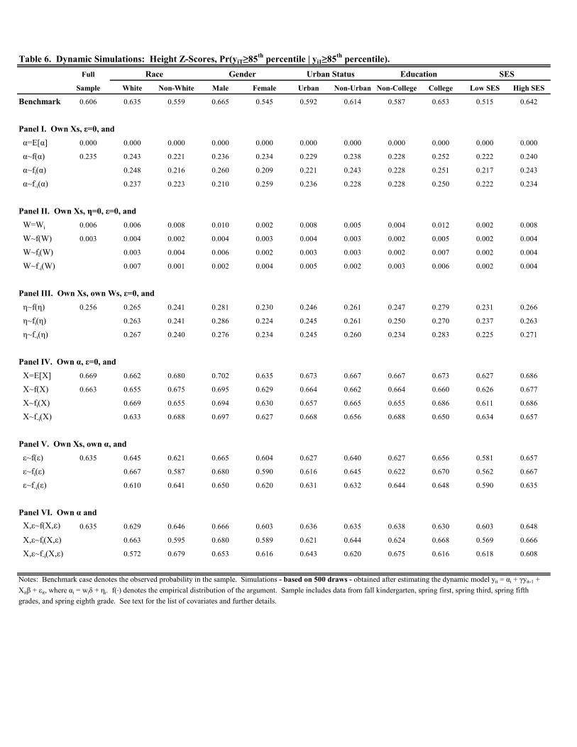
Table 6. Dynamic Simulations: Height Z-Scores, Pr(yiT≥85th percentile | yi1≥85th percentile).Full

Sample White Non-White Male Female Urban Non-Urban Non-College College Low SES High SES

Benchmark 0.606 0.635 0.559 0.665 0.545 0.592 0.614 0.587 0.653 0.515 0.642

Panel I. Own Xs, ε=0, and α=E[α] 0.000 0.000 0.000 0.000 0.000 0.000 0.000 0.000 0.000 0.000 0.000

α~f(α) 0.235 0.243 0.221 0.236 0.234 0.229 0.238 0.228 0.252 0.222 0.240

α~fi(α) 0.248 0.216 0.260 0.209 0.221 0.243 0.228 0.251 0.217 0.243

α~f-i(α) 0.237 0.223 0.210 0.259 0.236 0.228 0.228 0.250 0.222 0.234

Panel II. Own Xs, η=0, ε=0, and W=Wi 0.006 0.006 0.008 0.010 0.002 0.008 0.005 0.004 0.012 0.002 0.008

W~f(W) 0.003 0.004 0.002 0.004 0.003 0.004 0.003 0.002 0.005 0.002 0.004

W~fi(W) 0.003 0.004 0.006 0.002 0.003 0.003 0.002 0.007 0.002 0.004

W~f-i(W) 0.007 0.001 0.002 0.004 0.005 0.002 0.003 0.006 0.002 0.004

Panel III. Own Xs, own Ws, ε=0, and η~f(η) 0.256 0.265 0.241 0.281 0.230 0.246 0.261 0.247 0.279 0.231 0.266

η~fi(η) 0.263 0.241 0.286 0.224 0.245 0.261 0.250 0.270 0.237 0.263

η~f-i(η) 0.267 0.240 0.276 0.234 0.245 0.260 0.234 0.283 0.225 0.271

Panel IV. Own α, ε=0, and X=E[X] 0.669 0.662 0.680 0.702 0.635 0.673 0.667 0.667 0.673 0.627 0.686

X~f(X) 0.663 0.655 0.675 0.695 0.629 0.664 0.662 0.664 0.660 0.626 0.677

X~fi(X) 0.669 0.655 0.694 0.630 0.657 0.665 0.655 0.686 0.611 0.686

X~f-i(X) 0.633 0.688 0.697 0.627 0.668 0.656 0.688 0.650 0.634 0.657

Panel V. Own Xs, own α, and ε~f(ε) 0.635 0.645 0.621 0.665 0.604 0.627 0.640 0.627 0.656 0.581 0.657

ε~fi(ε) 0.667 0.587 0.680 0.590 0.616 0.645 0.622 0.670 0.562 0.667

ε~f-i(ε) 0.610 0.641 0.650 0.620 0.631 0.632 0.644 0.648 0.590 0.635

Panel VI. Own α and X,ε~f(X,ε) 0.635 0.629 0.646 0.666 0.603 0.636 0.635 0.638 0.630 0.603 0.648

X,ε~fi(X,ε) 0.663 0.595 0.680 0.589 0.621 0.644 0.624 0.668 0.569 0.666

X,ε~f-i(X,ε) 0.572 0.679 0.653 0.616 0.643 0.620 0.675 0.616 0.618 0.608

Notes: Benchmark case denotes the observed probability in the sample. Simulations - based on 500 draws - obtained after estimating the dynamic model yit = αi + γyit-1 + Xitβ + εit, where αi = wiδ + ηi. f(∙) denotes the empirical distribution of the argument. Sample includes data from fall kindergarten, spring first, spring third, spring fifth grades, and spring eighth grade. See text for the list of covariates and further details.

Race Gender Urban Status Education SES

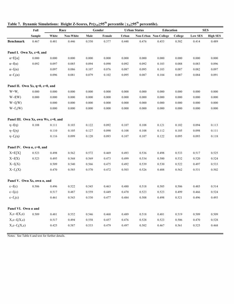
Table 7. Dynamic Simulations: Height Z-Scores, Pr(yiT≥95th percentile | yi1≥95th percentile).Full

Sample White Non-White Male Female Urban Non-Urban Non-College College Low SES High SES

Benchmark 0.467 0.481 0.446 0.550 0.377 0.448 0.476 0.453 0.502 0.414 0.489

Panel I. Own Xs, ε=0, and α=E[α] 0.000 0.000 0.000 0.000 0.000 0.000 0.000 0.000 0.000 0.000 0.000

α~f(α) 0.092 0.097 0.085 0.094 0.090 0.092 0.092 0.103 0.088 0.083 0.096

α~fi(α) 0.097 0.086 0.107 0.076 0.087 0.095 0.103 0.087 0.082 0.097

α~f-i(α) 0.096 0.081 0.079 0.102 0.095 0.087 0.104 0.087 0.084 0.091

Panel II. Own Xs, η=0, ε=0, and W=Wi 0.000 0.000 0.000 0.000 0.000 0.000 0.000 0.000 0.000 0.000 0.000

W~f(W) 0.000 0.000 0.000 0.000 0.000 0.000 0.000 0.000 0.000 0.000 0.000

W~fi(W) 0.000 0.000 0.000 0.000 0.000 0.000 0.000 0.000 0.000 0.000

W~f-i(W) 0.000 0.000 0.000 0.000 0.000 0.000 0.000 0.000 0.000 0.000

Panel III. Own Xs, own Ws, ε=0, and η~f(η) 0.108 0.111 0.103 0.122 0.092 0.107 0.108 0.121 0.102 0.094 0.113

η~fi(η) 0.110 0.105 0.127 0.090 0.108 0.108 0.112 0.105 0.098 0.111

η~f-i(η) 0.116 0.099 0.120 0.093 0.107 0.107 0.122 0.095 0.093 0.118

Panel IV. Own α, ε=0, and X=E[X] 0.523 0.498 0.562 0.572 0.469 0.493 0.536 0.498 0.533 0.517 0.525

X~f(X) 0.523 0.495 0.568 0.569 0.473 0.499 0.534 0.500 0.532 0.520 0.524

X~fi(X) 0.509 0.540 0.566 0.475 0.492 0.539 0.530 0.522 0.497 0.533

X~f-i(X) 0.470 0.585 0.570 0.472 0.503 0.526 0.488 0.562 0.531 0.502

Panel V. Own Xs, own α, and ε~f(ε) 0.506 0.496 0.522 0.545 0.463 0.480 0.518 0.505 0.506 0.485 0.514

ε~fi(ε) 0.517 0.487 0.559 0.449 0.470 0.523 0.523 0.499 0.466 0.524

ε~f-i(ε) 0.461 0.543 0.530 0.477 0.484 0.508 0.498 0.521 0.496 0.493

Panel VI. Own α and X,ε~f(X,ε) 0.509 0.481 0.552 0.546 0.468 0.489 0.518 0.481 0.519 0.509 0.509

X,ε~fi(X,ε) 0.517 0.494 0.558 0.457 0.476 0.528 0.523 0.506 0.470 0.528

X,ε~f-i(X,ε) 0.425 0.587 0.533 0.479 0.497 0.502 0.467 0.561 0.525 0.468

Race

Notes: See Table 6 and text for further details.

Gender Urban Status Education SES

Table 8. Dynamic Simulations: Height Z-Scores, Pr(yiT≥85th percentile | yi1≤50th percentile).Full

Sample White Non-White Male Female Urban Non-Urban Non-College College Low SES High SES

Benchmark 0.030 0.036 0.019 0.032 0.027 0.025 0.032 0.030 0.029 0.026 0.032

Panel I. Own Xs, ε=0, and α=E[α] 0.000 0.000 0.000 0.000 0.000 0.000 0.000 0.000 0.000 0.000 0.000

α~f(α) 0.144 0.151 0.134 0.144 0.145 0.141 0.146 0.158 0.140 0.136 0.149

α~fi(α) 0.153 0.135 0.163 0.126 0.134 0.151 0.157 0.141 0.134 0.150

α~f-i(α) 0.151 0.135 0.125 0.164 0.145 0.140 0.160 0.138 0.135 0.147

Panel II. Own Xs, η=0, ε=0, and W=Wi 0.000 0.000 0.000 0.000 0.000 0.000 0.000 0.000 0.000 0.000 0.000

W~f(W) 0.000 0.000 0.000 0.000 0.000 0.000 0.000 0.000 0.000 0.000 0.000

W~fi(W) 0.000 0.000 0.000 0.000 0.000 0.000 0.000 0.000 0.000 0.000

W~f-i(W) 0.000 0.000 0.000 0.000 0.000 0.000 0.000 0.000 0.000 0.000

Panel III. Own Xs, own Ws, ε=0, and η~f(η) 0.133 0.145 0.115 0.149 0.117 0.125 0.138 0.155 0.126 0.114 0.142

η~fi(η) 0.143 0.119 0.153 0.115 0.126 0.138 0.144 0.130 0.119 0.139

η~f-i(η) 0.149 0.114 0.145 0.120 0.125 0.139 0.159 0.118 0.112 0.149

Panel IV. Own α, ε=0, and X=E[X] 0.019 0.020 0.017 0.019 0.019 0.021 0.018 0.014 0.020 0.020 0.018

X~f(X) 0.018 0.019 0.016 0.017 0.018 0.019 0.017 0.014 0.019 0.019 0.017

X~fi(X) 0.020 0.014 0.017 0.018 0.018 0.017 0.015 0.018 0.018 0.018

X~f-i(X) 0.017 0.017 0.017 0.018 0.019 0.017 0.013 0.021 0.020 0.015

Panel V. Own Xs, own α, and ε~f(ε) 0.021 0.024 0.016 0.022 0.020 0.021 0.021 0.021 0.021 0.021 0.021

ε~fi(ε) 0.026 0.014 0.022 0.020 0.020 0.021 0.023 0.020 0.019 0.022

ε~f-i(ε) 0.021 0.018 0.021 0.020 0.021 0.020 0.021 0.023 0.021 0.019

Panel VI. Own α and X,ε~f(X,ε) 0.022 0.024 0.019 0.023 0.021 0.023 0.022 0.019 0.023 0.023 0.022

X,ε~fi(X,ε) 0.027 0.015 0.023 0.021 0.022 0.022 0.024 0.021 0.020 0.023

X,ε~f-i(X,ε) 0.019 0.022 0.023 0.021 0.023 0.021 0.018 0.028 0.024 0.018

Notes: See Table 6 and text for further details.

Gender Urban Status Education SESRace

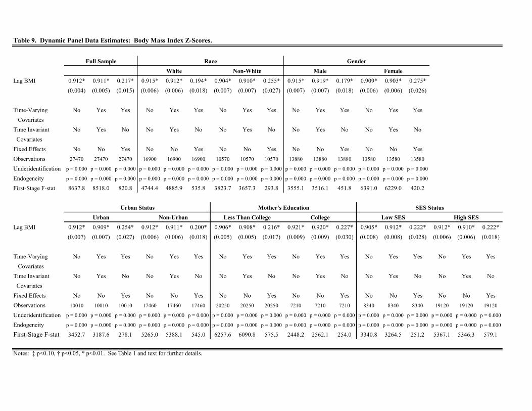
Table 9. Dynamic Panel Data Estimates: Body Mass Index Z-Scores.

Lag BMI 0.912* 0.911* 0.217* 0.915* 0.912* 0.194* 0.904* 0.910* 0.255* 0.915* 0.919* 0.179* 0.909* 0.903* 0.275*(0.004) (0.005) (0.015) (0.006) (0.006) (0.018) (0.007) (0.007) (0.027) (0.007) (0.007) (0.018) (0.006) (0.006) (0.026)

Time-Varying No Yes Yes No Yes Yes No Yes Yes No Yes Yes No Yes Yes CovariatesTime Invariant No Yes No No Yes No No Yes No No Yes No No Yes No CovariatesFixed Effects No No Yes No No Yes No No Yes No No Yes No No YesObservations 27470 27470 27470 16900 16900 16900 10570 10570 10570 13880 13880 13880 13580 13580 13580

Underidentification p = 0.000 p = 0.000 p = 0.000 p = 0.000 p = 0.000 p = 0.000 p = 0.000 p = 0.000 p = 0.000 p = 0.000 p = 0.000 p = 0.000 p = 0.000 p = 0.000 p = 0.000

Endogeneity p = 0.000 p = 0.000 p = 0.000 p = 0.000 p = 0.000 p = 0.000 p = 0.000 p = 0.000 p = 0.000 p = 0.000 p = 0.000 p = 0.000 p = 0.000 p = 0.000 p = 0.000

First-Stage F-stat 8637.8 8518.0 820.8 4744.4 4885.9 535.8 3823.7 3657.3 293.8 3555.1 3516.1 451.8 6391.0 6229.0 420.2

Lag BMI 0.912* 0.909* 0.254* 0.912* 0.911* 0.200* 0.906* 0.908* 0.216* 0.921* 0.920* 0.227* 0.905* 0.912* 0.222* 0.912* 0.910* 0.222*(0.007) (0.007) (0.027) (0.006) (0.006) (0.018) (0.005) (0.005) (0.017) (0.009) (0.009) (0.030) (0.008) (0.008) (0.028) (0.006) (0.006) (0.018)

Time-Varying No Yes Yes No Yes Yes No Yes Yes No Yes Yes No Yes Yes No Yes Yes CovariatesTime Invariant No Yes No No Yes No No Yes No No Yes No No Yes No No Yes No CovariatesFixed Effects No No Yes No No Yes No No Yes No No Yes No No Yes No No YesObservations 10010 10010 10010 17460 17460 17460 20250 20250 20250 7210 7210 7210 8340 8340 8340 19120 19120 19120

Underidentification p = 0.000 p = 0.000 p = 0.000 p = 0.000 p = 0.000 p = 0.000 p = 0.000 p = 0.000 p = 0.000 p = 0.000 p = 0.000 p = 0.000 p = 0.000 p = 0.000 p = 0.000 p = 0.000 p = 0.000 p = 0.000

Endogeneity p = 0.000 p = 0.000 p = 0.000 p = 0.000 p = 0.000 p = 0.000 p = 0.000 p = 0.000 p = 0.000 p = 0.000 p = 0.000 p = 0.000 p = 0.000 p = 0.000 p = 0.000 p = 0.000 p = 0.000 p = 0.000

First-Stage F-stat 3452.7 3187.6 278.1 5265.0 5388.1 545.0 6257.6 6090.8 575.5 2448.2 2562.1 254.0 3340.8 3264.5 251.2 5367.1 5346.3 579.1

Race GenderWhite Non-White Male Female

Full Sample

Notes: ‡ p<0.10, † p<0.05, * p<0.01. See Table 1 and text for further details.

Urban Status Mother's Education SES StatusUrban Non-Urban Less Than College College Low SES High SES

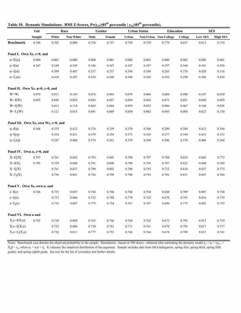
Table 10. Dynamic Simulations: BMI Z-Scores, Pr(yiT≥85th percentile | yi1≥85th percentile).Full

Sample White Non-White Male Female Urban Non-Urban Non-College College Low SES High SES

Benchmark 0.746 0.703 0.800 0.736 0.757 0.758 0.739 0.779 0.637 0.813 0.710

Panel I. Own Xs, ε=0, and α=E[α] 0.000 0.001 0.000 0.000 0.001 0.000 0.001 0.000 0.002 0.000 0.001

α~f(α) 0.347 0.348 0.345 0.346 0.347 0.347 0.347 0.357 0.344 0.341 0.350

α~fi(α) 0.309 0.407 0.357 0.337 0.344 0.348 0.265 0.376 0.420 0.316

α~f-i(α) 0.410 0.307 0.334 0.360 0.348 0.345 0.392 0.250 0.306 0.430

Panel II. Own Xs, η=0, ε=0, and W=Wi 0.070 0.011 0.145 0.076 0.065 0.079 0.066 0.004 0.090 0.147 0.030

W~f(W) 0.055 0.056 0.055 0.054 0.057 0.054 0.056 0.071 0.051 0.049 0.059

W~fi(W) 0.015 0.118 0.065 0.044 0.059 0.052 0.006 0.067 0.108 0.028

W~f-i(W) 0.121 0.015 0.041 0.069 0.050 0.062 0.093 0.004 0.023 0.130

Panel III. Own Xs, own Ws, ε=0, and η~f(η) 0.368 0.333 0.412 0.376 0.359 0.370 0.366 0.299 0.389 0.413 0.344

η~fi(η) 0.324 0.421 0.379 0.356 0.373 0.365 0.277 0.394 0.433 0.333

η~f-i(η) 0.347 0.406 0.374 0.363 0.370 0.369 0.306 0.378 0.406 0.364

Panel IV. Own α, ε=0, and X=E[X] 0.797 0.761 0.842 0.793 0.802 0.798 0.797 0.708 0.824 0.845 0.772

X~f(X) 0.795 0.759 0.840 0.791 0.800 0.798 0.793 0.707 0.822 0.844 0.769

X~fi(X) 0.761 0.837 0.789 0.802 0.798 0.793 0.723 0.818 0.837 0.773

X~f-i(X) 0.756 0.841 0.792 0.798 0.798 0.793 0.701 0.831 0.847 0.760

Panel V. Own Xs, own α, and ε~f(ε) 0.766 0.733 0.807 0.764 0.768 0.768 0.764 0.688 0.789 0.807 0.744

ε~fi(ε) 0.733 0.806 0.752 0.780 0.770 0.762 0.670 0.793 0.816 0.739

ε~f-i(ε) 0.732 0.807 0.775 0.754 0.767 0.767 0.696 0.775 0.802 0.755

Panel VI. Own α and X,ε~f(X,ε) 0.765 0.730 0.808 0.763 0.766 0.768 0.762 0.672 0.792 0.813 0.739

X,ε~fi(X,ε) 0.732 0.806 0.750 0.781 0.771 0.761 0.670 0.793 0.817 0.737

X,ε~f-i(X,ε) 0.726 0.811 0.777 0.752 0.768 0.764 0.674 0.789 0.812 0.741

Notes: Benchmark case denotes the observed probability in the sample. Simulations - based on 500 draws - obtained after estimating the dynamic model yit = αi + γyit-1 + Xitβ + εit, where αi = wiδ + ηi. f(∙) denotes the empirical distribution of the argument. Sample includes data from fall kindergarten, spring first, spring third, spring fifth grades, and spring eighth grade. See text for the list of covariates and further details.

Race Gender Urban Status Education SES

Table 11. Dynamic Simulations: BMI Z-Scores, Pr(yiT≥95th percentile | yi1≥95th percentile).Full

Sample White Non-White Male Female Urban Non-Urban Non-College College Low SES High SES

Benchmark 0.715 0.664 0.769 0.724 0.703 0.738 0.702 0.757 0.538 0.783 0.672

Panel I. Own Xs, ε=0, and α=E[α] 0.000 0.000 0.000 0.000 0.000 0.000 0.000 0.000 0.000 0.000 0.000

α~f(α) 0.179 0.180 0.178 0.178 0.180 0.177 0.179 0.187 0.177 0.175 0.181

α~fi(α) 0.147 0.228 0.194 0.161 0.181 0.176 0.117 0.199 0.233 0.153

α~f-i(α) 0.231 0.144 0.158 0.196 0.176 0.179 0.211 0.109 0.149 0.242

Panel II. Own Xs, η=0, ε=0, and W=Wi 0.000 0.000 0.000 0.000 0.000 0.000 0.000 0.000 0.000 0.000 0.000

W~f(W) 0.000 0.000 0.000 0.000 0.000 0.000 0.000 0.000 0.000 0.000 0.000

W~fi(W) 0.000 0.000 0.000 0.000 0.000 0.000 0.000 0.000 0.000 0.000

W~f-i(W) 0.000 0.000 0.000 0.000 0.000 0.000 0.000 0.000 0.000 0.000

Panel III. Own Xs, own Ws, ε=0, and η~f(η) 0.195 0.171 0.221 0.199 0.190 0.195 0.196 0.137 0.209 0.226 0.176

η~fi(η) 0.162 0.238 0.207 0.182 0.198 0.193 0.124 0.216 0.244 0.168

η~f-i(η) 0.184 0.212 0.192 0.197 0.194 0.198 0.142 0.190 0.217 0.193

Panel IV. Own α, ε=0, and X=E[X] 0.792 0.757 0.830 0.804 0.778 0.810 0.782 0.629 0.832 0.845 0.759

X~f(X) 0.792 0.758 0.827 0.802 0.778 0.808 0.782 0.628 0.831 0.841 0.761

X~fi(X) 0.760 0.824 0.801 0.781 0.808 0.783 0.648 0.826 0.830 0.766

X~f-i(X) 0.754 0.830 0.805 0.776 0.809 0.782 0.622 0.845 0.846 0.749

Panel V. Own Xs, own α, and ε~f(ε) 0.734 0.699 0.771 0.739 0.728 0.748 0.726 0.597 0.767 0.776 0.708

ε~fi(ε) 0.698 0.770 0.723 0.746 0.752 0.724 0.575 0.774 0.788 0.700

ε~f-i(ε) 0.698 0.771 0.755 0.710 0.747 0.729 0.606 0.747 0.770 0.721

Panel VI. Own α and X,ε~f(X,ε) 0.735 0.699 0.773 0.742 0.726 0.749 0.727 0.583 0.771 0.784 0.704

X,ε~fi(X,ε) 0.700 0.770 0.724 0.743 0.750 0.727 0.579 0.772 0.787 0.702

X,ε~f-i(X,ε) 0.694 0.775 0.761 0.706 0.749 0.729 0.583 0.767 0.783 0.706

Urban Status Education SES

Notes: See Table 10 and text for further details.

Race Gender

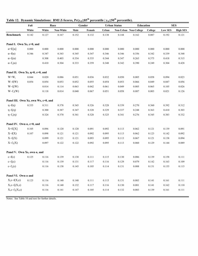
Table 12. Dynamic Simulations: BMI Z-Scores, Pr(yiT≥85th percentile | yi1≤50th percentile).Full

White White Non-White Male Female Urban Non-Urban Non-College College Low SES High SES

Benchmark 0.142 0.127 0.167 0.152 0.132 0.138 0.144 0.162 0.087 0.192 0.121

Panel I. Own Xs, ε=0, and α=E[α] 0.000 0.000 0.000 0.000 0.000 0.000 0.000 0.000 0.000 0.000 0.000

α~f(α) 0.346 0.347 0.343 0.345 0.347 0.346 0.346 0.356 0.342 0.339 0.348

α~fi(α) 0.308 0.403 0.354 0.335 0.344 0.347 0.263 0.375 0.418 0.315

α~f-i(α) 0.410 0.304 0.333 0.359 0.348 0.342 0.390 0.249 0.304 0.428

Panel II. Own Xs, η=0, ε=0, and W=Wi 0.044 0.020 0.086 0.051 0.036 0.032 0.050 0.005 0.058 0.094 0.023

W~f(W) 0.054 0.054 0.053 0.052 0.055 0.054 0.053 0.066 0.049 0.047 0.056

W~fi(W) 0.014 0.114 0.063 0.042 0.061 0.049 0.005 0.065 0.105 0.026

W~f-i(W) 0.118 0.014 0.040 0.067 0.051 0.058 0.087 0.003 0.021 0.126

Panel III. Own Xs, own Ws, ε=0, and η~f(η) 0.335 0.311 0.378 0.345 0.326 0.328 0.339 0.270 0.360 0.392 0.312

η~fi(η) 0.300 0.387 0.347 0.320 0.329 0.337 0.248 0.363 0.410 0.303

η~f-i(η) 0.324 0.370 0.341 0.328 0.325 0.341 0.276 0.345 0.383 0.332

Panel IV. Own α, ε=0, and X=E[X] 0.105 0.096 0.120 0.120 0.091 0.092 0.113 0.062 0.121 0.139 0.091

X~f(X) 0.107 0.098 0.121 0.121 0.092 0.095 0.113 0.062 0.123 0.142 0.092

X~fi(X) 0.099 0.121 0.121 0.093 0.095 0.113 0.067 0.121 0.138 0.094

X~f-i(X) 0.097 0.122 0.122 0.092 0.095 0.113 0.060 0.129 0.144 0.089

Panel V. Own Xs, own α, and ε~f(ε) 0.125 0.116 0.139 0.138 0.111 0.115 0.130 0.086 0.139 0.158 0.111

ε~fi(ε) 0.116 0.139 0.131 0.117 0.116 0.129 0.079 0.142 0.163 0.109

ε~f-i(ε) 0.116 0.138 0.145 0.105 0.114 0.131 0.088 0.131 0.155 0.115

Panel VI. Own α and X,ε~f(X,ε) 0.125 0.116 0.140 0.140 0.111 0.115 0.131 0.083 0.141 0.161 0.111

X,ε~fi(X,ε) 0.116 0.140 0.132 0.117 0.116 0.130 0.081 0.141 0.162 0.110

X,ε~f-i(X,ε) 0.116 0.141 0.147 0.105 0.114 0.132 0.083 0.139 0.161 0.111

Urban Status Education SES

Notes: See Table 10 and text for further details.

Race Gender

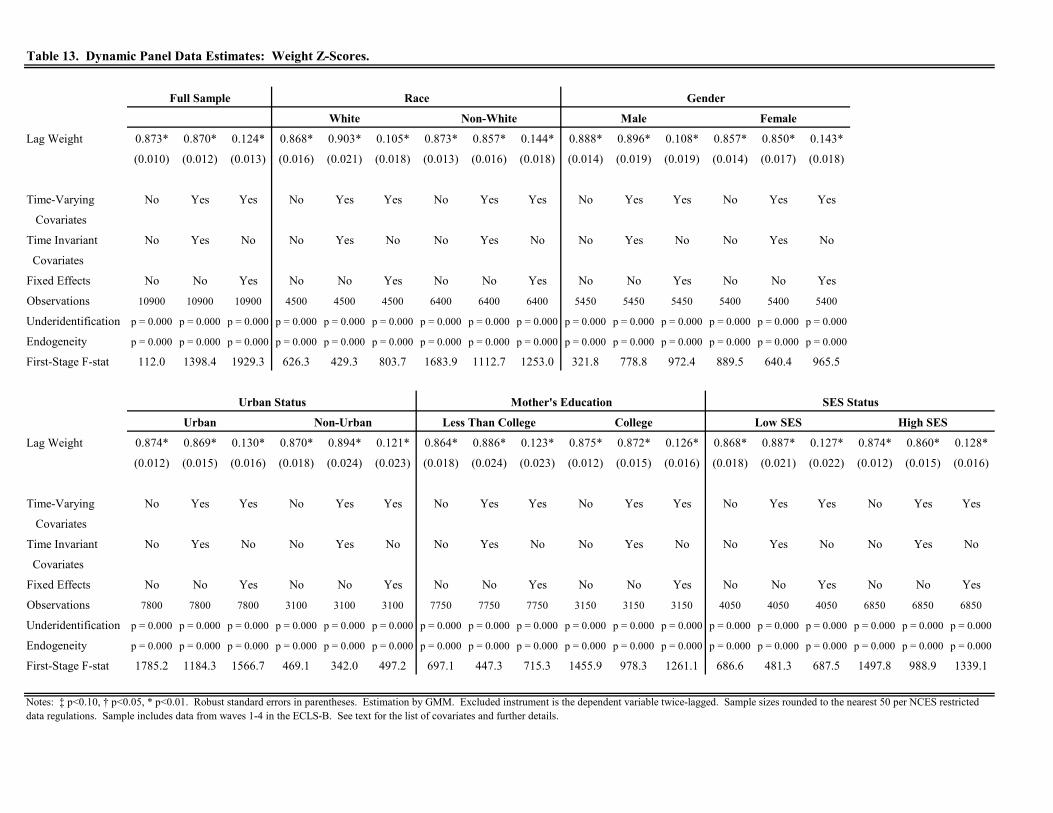
Table 13. Dynamic Panel Data Estimates: Weight Z-Scores.

Lag Weight 0.873* 0.870* 0.124* 0.868* 0.903* 0.105* 0.873* 0.857* 0.144* 0.888* 0.896* 0.108* 0.857* 0.850* 0.143*

(0.010) (0.012) (0.013) (0.016) (0.021) (0.018) (0.013) (0.016) (0.018) (0.014) (0.019) (0.019) (0.014) (0.017) (0.018)

Time-Varying No Yes Yes No Yes Yes No Yes Yes No Yes Yes No Yes Yes

Covariates

Time Invariant No Yes No No Yes No No Yes No No Yes No No Yes No

Covariates

Fixed Effects No No Yes No No Yes No No Yes No No Yes No No Yes

Observations 10900 10900 10900 4500 4500 4500 6400 6400 6400 5450 5450 5450 5400 5400 5400

Underidentification p = 0.000 p = 0.000 p = 0.000 p = 0.000 p = 0.000 p = 0.000 p = 0.000 p = 0.000 p = 0.000 p = 0.000 p = 0.000 p = 0.000 p = 0.000 p = 0.000 p = 0.000

Endogeneity p = 0.000 p = 0.000 p = 0.000 p = 0.000 p = 0.000 p = 0.000 p = 0.000 p = 0.000 p = 0.000 p = 0.000 p = 0.000 p = 0.000 p = 0.000 p = 0.000 p = 0.000

First-Stage F-stat 112.0 1398.4 1929.3 626.3 429.3 803.7 1683.9 1112.7 1253.0 321.8 778.8 972.4 889.5 640.4 965.5

Lag Weight 0.874* 0.869* 0.130* 0.870* 0.894* 0.121* 0.864* 0.886* 0.123* 0.875* 0.872* 0.126* 0.868* 0.887* 0.127* 0.874* 0.860* 0.128*

(0.012) (0.015) (0.016) (0.018) (0.024) (0.023) (0.018) (0.024) (0.023) (0.012) (0.015) (0.016) (0.018) (0.021) (0.022) (0.012) (0.015) (0.016)

Time-Varying No Yes Yes No Yes Yes No Yes Yes No Yes Yes No Yes Yes No Yes Yes

Covariates

Time Invariant No Yes No No Yes No No Yes No No Yes No No Yes No No Yes No

Covariates

Fixed Effects No No Yes No No Yes No No Yes No No Yes No No Yes No No Yes

Observations 7800 7800 7800 3100 3100 3100 7750 7750 7750 3150 3150 3150 4050 4050 4050 6850 6850 6850

Underidentification p = 0.000 p = 0.000 p = 0.000 p = 0.000 p = 0.000 p = 0.000 p = 0.000 p = 0.000 p = 0.000 p = 0.000 p = 0.000 p = 0.000 p = 0.000 p = 0.000 p = 0.000 p = 0.000 p = 0.000 p = 0.000

Endogeneity p = 0.000 p = 0.000 p = 0.000 p = 0.000 p = 0.000 p = 0.000 p = 0.000 p = 0.000 p = 0.000 p = 0.000 p = 0.000 p = 0.000 p = 0.000 p = 0.000 p = 0.000 p = 0.000 p = 0.000 p = 0.000

First-Stage F-stat 1785.2 1184.3 1566.7 469.1 342.0 497.2 697.1 447.3 715.3 1455.9 978.3 1261.1 686.6 481.3 687.5 1497.8 988.9 1339.1

Full Sample Race Gender

Urban Status Mother's Education SES Status

White Non-White Male Female

High SES

Notes: ‡ p<0.10, † p<0.05, * p<0.01. Robust standard errors in parentheses. Estimation by GMM. Excluded instrument is the dependent variable twice-lagged. Sample sizes rounded to the nearest 50 per NCES restricted data regulations. Sample includes data from waves 1-4 in the ECLS-B. See text for the list of covariates and further details.

Urban Non-Urban Less Than College College Low SES

Table 14. Dynamic Simulations: Weight Z-Scores, Pr(yiT≥85th percentile | yi1≥85th percentile).Full

Sample White Non-White Male Female Urban Non-Urban Non-College College Low SES High SES

Benchmark 0.541 0.508 0.558 0.605 0.496 0.511 0.621 0.434 0.583 0.593 0.507

Panel I. Own Xs, ε=0, and α=E[α] 0.007 0.000 0.010 0.005 0.008 0.006 0.008 0.000 0.009 0.014 0.002 α~f(α) 0.255 0.284 0.240 0.249 0.259 0.240 0.295 0.237 0.262 0.257 0.254 α~fi(α) 0.216 0.284 0.263 0.243 0.248 0.267 0.213 0.271 0.285 0.237 α~f-i(α) 0.333 0.180 0.234 0.275 0.217 0.308 0.246 0.242 0.240 0.284

Panel II. Own Xs, η=0, ε=0, and W=Wi 0.169 0.135 0.187 0.181 0.161 0.157 0.202 0.112 0.191 0.174 0.166 W~f(W) 0.101 0.120 0.092 0.090 0.109 0.085 0.142 0.080 0.109 0.106 0.098 W~fi(W) 0.050 0.127 0.103 0.094 0.094 0.107 0.068 0.115 0.122 0.087 W~f-i(W) 0.166 0.042 0.078 0.121 0.064 0.154 0.086 0.093 0.096 0.114

Panel III. Own Xs, own Ws, ε=0, and η~f(η) 0.332 0.311 0.343 0.340 0.326 0.322 0.358 0.304 0.343 0.338 0.328 η~fi(η) 0.307 0.347 0.344 0.326 0.324 0.354 0.294 0.348 0.357 0.318 η~f-i(η) 0.320 0.337 0.340 0.327 0.320 0.361 0.309 0.336 0.328 0.346

Panel IV. Own α, ε=0, and X=E[X] 0.605 0.532 0.642 0.678 0.554 0.593 0.637 0.558 0.624 0.646 0.578 X~f(X) 0.596 0.521 0.634 0.659 0.552 0.591 0.611 0.557 0.612 0.630 0.574 X~fi(X) 0.560 0.609 0.656 0.557 0.576 0.652 0.525 0.623 0.639 0.568 X~f-i(X) 0.494 0.670 0.662 0.550 0.630 0.593 0.570 0.585 0.628 0.582

Panel V. Own Xs, own α, and ε~f(ε) 0.581 0.556 0.594 0.635 0.543 0.556 0.649 0.516 0.607 0.611 0.562 ε~fi(ε) 0.553 0.595 0.630 0.547 0.553 0.653 0.511 0.607 0.616 0.557 ε~f-i(ε) 0.558 0.592 0.640 0.538 0.560 0.647 0.520 0.603 0.608 0.567

Panel VI. Own α and X,ε~f(X,ε) 0.582 0.509 0.618 0.633 0.546 0.578 0.593 0.546 0.596 0.615 0.561 X,ε~fi(X,ε) 0.541 0.596 0.626 0.554 0.564 0.634 0.510 0.609 0.625 0.553 X,ε~f-i(X,ε) 0.486 0.652 0.641 0.539 0.618 0.577 0.559 0.566 0.609 0.574

Notes: Benchmark case denotes the observed probability in the sample. Simulations - based on 500 draws - obtained after estimating the dynamic model yit = αi + γyit-1 + Xitβ + εit, where αi = wiδ + ηi. f(∙) denotes the empirical distribution of the argument. Sample includes data from waves 1-4 of the ECLS-B. See text for the list of covariates and further details.

Race Gender Urban Status Education SES

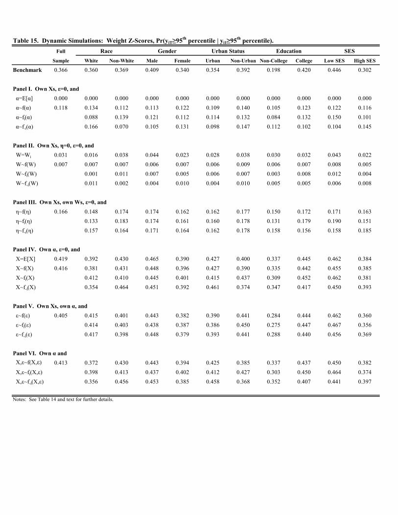
Table 15. Dynamic Simulations: Weight Z-Scores, Pr(yiT≥95th percentile | yi1≥95th percentile).Full

Sample White Non-White Male Female Urban Non-Urban Non-College College Low SES High SES

Benchmark 0.366 0.360 0.369 0.409 0.340 0.354 0.392 0.198 0.420 0.446 0.302

Panel I. Own Xs, ε=0, and α=E[α] 0.000 0.000 0.000 0.000 0.000 0.000 0.000 0.000 0.000 0.000 0.000 α~f(α) 0.118 0.134 0.112 0.113 0.122 0.109 0.140 0.105 0.123 0.122 0.116 α~fi(α) 0.088 0.139 0.121 0.112 0.114 0.132 0.084 0.132 0.150 0.101 α~f-i(α) 0.166 0.070 0.105 0.131 0.098 0.147 0.112 0.102 0.104 0.145

Panel II. Own Xs, η=0, ε=0, and W=Wi 0.031 0.016 0.038 0.044 0.023 0.028 0.038 0.030 0.032 0.043 0.022 W~f(W) 0.007 0.007 0.007 0.006 0.007 0.006 0.009 0.006 0.007 0.008 0.005 W~fi(W) 0.001 0.011 0.007 0.005 0.006 0.007 0.003 0.008 0.012 0.004 W~f-i(W) 0.011 0.002 0.004 0.010 0.004 0.010 0.005 0.005 0.006 0.008

Panel III. Own Xs, own Ws, ε=0, and η~f(η) 0.166 0.148 0.174 0.174 0.162 0.162 0.177 0.150 0.172 0.171 0.163 η~fi(η) 0.133 0.183 0.174 0.161 0.160 0.178 0.131 0.179 0.190 0.151 η~f-i(η) 0.157 0.164 0.171 0.164 0.162 0.178 0.158 0.156 0.158 0.185

Panel IV. Own α, ε=0, and X=E[X] 0.419 0.392 0.430 0.465 0.390 0.427 0.400 0.337 0.445 0.462 0.384 X~f(X) 0.416 0.381 0.431 0.448 0.396 0.427 0.390 0.335 0.442 0.455 0.385 X~fi(X) 0.412 0.410 0.445 0.401 0.415 0.437 0.309 0.452 0.462 0.381 X~f-i(X) 0.354 0.464 0.451 0.392 0.461 0.374 0.347 0.417 0.450 0.393

Panel V. Own Xs, own α, and ε~f(ε) 0.405 0.415 0.401 0.443 0.382 0.390 0.441 0.284 0.444 0.462 0.360 ε~fi(ε) 0.414 0.403 0.438 0.387 0.386 0.450 0.275 0.447 0.467 0.356 ε~f-i(ε) 0.417 0.398 0.448 0.379 0.393 0.441 0.288 0.440 0.456 0.369

Panel VI. Own α and X,ε~f(X,ε) 0.413 0.372 0.430 0.443 0.394 0.425 0.385 0.337 0.437 0.450 0.382 X,ε~fi(X,ε) 0.398 0.413 0.437 0.402 0.412 0.427 0.303 0.450 0.464 0.374 X,ε~f-i(X,ε) 0.356 0.456 0.453 0.385 0.458 0.368 0.352 0.407 0.441 0.397

Notes: See Table 14 and text for further details.

Race Gender Urban Status Education SES

Table 16. Dynamic Simulations: Weight Z-Scores, Pr(yiT≥85th percentile | yi1≤50th percentile).Full

Sample White Non-White Male Female Urban Non-Urban Non-College College Low SES High SES

Benchmark 0.431 0.426 0.435 0.443 0.418 0.426 0.443 0.395 0.446 0.468 0.410

Panel I. Own Xs, ε=0, and α=E[α] 0.837 0.982 0.724 0.830 0.846 0.793 0.949 0.798 0.854 0.820 0.847 α~f(α) 0.617 0.646 0.593 0.614 0.619 0.605 0.645 0.594 0.626 0.627 0.610 α~fi(α) 0.594 0.632 0.624 0.610 0.614 0.622 0.592 0.627 0.635 0.606 α~f-i(α) 0.683 0.537 0.603 0.629 0.579 0.653 0.594 0.626 0.622 0.619

Panel II. Own Xs, η=0, ε=0, and W=Wi 0.613 0.553 0.661 0.633 0.591 0.613 0.615 0.559 0.636 0.648 0.594 W~f(W) 0.719 0.777 0.674 0.715 0.725 0.698 0.771 0.685 0.734 0.732 0.712 W~fi(W) 0.680 0.749 0.734 0.706 0.715 0.737 0.676 0.737 0.740 0.708 W~f-i(W) 0.847 0.566 0.696 0.743 0.659 0.784 0.688 0.727 0.726 0.721

Panel III. Own Xs, own Ws, ε=0, and η~f(η) 0.556 0.525 0.581 0.568 0.542 0.556 0.555 0.526 0.568 0.574 0.546 η~fi(η) 0.527 0.577 0.569 0.543 0.559 0.551 0.532 0.567 0.578 0.543 η~f-i(η) 0.523 0.585 0.570 0.541 0.552 0.557 0.525 0.575 0.572 0.551

Panel IV. Own α, ε=0, and X=E[X] 0.435 0.398 0.465 0.462 0.405 0.447 0.407 0.444 0.432 0.432 0.437 X~f(X) 0.440 0.401 0.470 0.464 0.412 0.451 0.413 0.442 0.439 0.442 0.439 X~fi(X) 0.436 0.448 0.460 0.416 0.436 0.452 0.413 0.450 0.451 0.434 X~f-i(X) 0.377 0.503 0.467 0.410 0.488 0.397 0.455 0.411 0.436 0.447

Panel V. Own Xs, own α, and ε~f(ε) 0.431 0.428 0.434 0.453 0.407 0.429 0.436 0.402 0.444 0.450 0.421 ε~fi(ε) 0.425 0.437 0.449 0.411 0.428 0.440 0.396 0.446 0.458 0.417 ε~f-i(ε) 0.431 0.430 0.457 0.403 0.435 0.434 0.405 0.438 0.447 0.429

Panel VI. Own α and X,ε~f(X,ε) 0.441 0.405 0.469 0.464 0.415 0.451 0.417 0.442 0.441 0.445 0.439 X,ε~fi(X,ε) 0.431 0.451 0.457 0.423 0.436 0.455 0.408 0.454 0.460 0.429 X,ε~f-i(X,ε) 0.387 0.496 0.472 0.407 0.488 0.401 0.456 0.410 0.437 0.454

Notes: See Table 14 and text for further details.

Race Gender Urban Status Education SES

Table 17. Dynamic Panel Data Estimates: Height.

Lag Height 0.480* 0.506* -0.002 0.488* 0.522* 0.002 0.474* 0.493* -0.005 0.485* 0.511* -0.056* 0.474* 0.498* -0.043*(0.004) (0.010) (0.007) (0.006) (0.016) (0.012) (0.005) (0.013) (0.009) (0.006) (0.014) (0.008) (0.006) (0.015) (0.008)

Time-Varying No Yes Yes No Yes Yes No Yes Yes No Yes Yes No Yes Yes CovariatesTime Invariant No Yes No No Yes No No Yes No No Yes No No Yes No CovariatesFixed Effects No No Yes No No Yes No No Yes No No Yes No No YesObservations 10900 10900 10900 4500 4500 4500 6400 6400 6400 5450 5450 5450 5400 5400 5400

Underidentification p = 0.000 p = 0.000 p = 0.000 p = 0.000 p = 0.000 p = 0.000 p = 0.000 p = 0.000 p = 0.000 p = 0.000 p = 0.000 p = 0.000 p = 0.000 p = 0.000 p = 0.000

Endogeneity p = 0.000 p = 0.000 p = 0.000 p = 0.000 p = 0.000 p = 0.000 p = 0.000 p = 0.000 p = 0.000 p = 0.000 p = 0.000 p = 0.000 p = 0.000 p = 0.000 p = 0.000

First-Stage F-stat 770.2 6940.2 10250.2 17737.1 2263.8 3947.3 27111.7 4758.6 6311.6 568.9 3435.1 8396.2 21349.5 3328.9 8158.5

Lag Height 0.475* 0.491* -0.049* 0.493* 0.549* -0.057* 0.481* 0.492* -0.051* 0.480* 0.515* -0.049* 0.466* 0.486* -0.055* 0.488* 0.524* -0.045*(0.005) (0.012) (0.007) (0.008) (0.021) (0.011) (0.007) (0.018) (0.010) (0.005) (0.012) (0.007) (0.007) (0.017) (0.009) (0.005) (0.013) (0.007)

Time-Varying No Yes Yes No Yes Yes No Yes Yes No Yes Yes No Yes Yes No Yes Yes CovariatesTime Invariant No Yes No No Yes No No Yes No No Yes No No Yes No No Yes No CovariatesFixed Effects No No Yes No No Yes No No Yes No No Yes No No Yes No No YesObservations 7800 7800 7800 3100 3100 3100 7750 7750 7750 3150 3150 3150 4050 4050 4050 6850 6850 6850

Underidentification p = 0.000 p = 0.000 p = 0.000 p = 0.000 p = 0.000 p = 0.000 p = 0.000 p = 0.000 p = 0.000 p = 0.000 p = 0.000 p = 0.000 p = 0.000 p = 0.000 p = 0.000 p = 0.000 p = 0.000 p = 0.000

Endogeneity p = 0.000 p = 0.000 p = 0.000 p = 0.000 p = 0.000 p = 0.000 p = 0.000 p = 0.000 p = 0.000 p = 0.006 p = 0.000 p = 0.000 p = 0.000 p = 0.000 p = 0.000 p = 0.000 p = 0.000 p = 0.000

First-Stage F-stat 33778.2 5408.6 12465.7 310.8 1489.6 3939.6 13369.8 1660.6 4565.1 31408.3 5230.3 11710.0 246.8 2752.0 6982.2 28553.6 4057.3 9316.1

Less Than College College Low SES

Notes: ‡ p<0.10, † p<0.05, * p<0.01. Dependent variable is length/height in centimeters. See Table 13 and text for further details.

GenderFull Sample RaceWhite Non-White Male Female

Urban Status Mother's Education SES StatusHigh SESUrban Non-Urban

Table 18. Dynamic Simulations: Height, Pr(yiT≥85th percentile | yi1≥85th percentile).Full

Sample White Non-White Male Female Urban Non-Urban Non-College College Low SES High SES

Benchmark 0.600 0.576 0.615 0.626 0.580 0.611 0.574 0.585 0.606 0.605 0.598

Panel I. Own Xs, ε=0, and α=E[α] 0.190 0.225 0.169 0.062 0.292 0.175 0.228 0.135 0.213 0.198 0.186 α~f(α) 0.380 0.400 0.368 0.332 0.418 0.373 0.397 0.355 0.390 0.387 0.376 α~fi(α) 0.351 0.403 0.368 0.381 0.385 0.368 0.377 0.381 0.383 0.379 α~f-i(α) 0.435 0.318 0.295 0.456 0.342 0.410 0.345 0.416 0.392 0.369

Panel II. Own Xs, η=0, ε=0, and W=Wi 0.396 0.367 0.413 0.386 0.403 0.401 0.383 0.386 0.400 0.373 0.409 W~f(W) 0.292 0.323 0.274 0.210 0.357 0.281 0.320 0.252 0.308 0.306 0.284 W~fi(W) 0.256 0.316 0.258 0.300 0.301 0.266 0.275 0.297 0.284 0.296 W~f-i(W) 0.370 0.215 0.163 0.414 0.232 0.340 0.242 0.335 0.319 0.264

Panel III. Own Xs, own Ws, ε=0, and η~f(η) 0.444 0.430 0.452 0.438 0.448 0.447 0.435 0.437 0.446 0.438 0.447 η~fi(η) 0.430 0.451 0.439 0.447 0.447 0.436 0.449 0.441 0.447 0.442 η~f-i(η) 0.431 0.450 0.437 0.449 0.445 0.436 0.433 0.457 0.433 0.456

Panel IV. Own α, ε=0, and X=E[X] 0.607 0.565 0.632 0.622 0.594 0.623 0.568 0.630 0.597 0.591 0.616 X~f(X) 0.597 0.564 0.616 0.607 0.588 0.612 0.559 0.622 0.586 0.589 0.601 X~fi(X) 0.581 0.605 0.605 0.591 0.606 0.575 0.595 0.598 0.597 0.596 X~f-i(X) 0.554 0.633 0.608 0.587 0.630 0.551 0.634 0.556 0.584 0.610

Panel V. Own Xs, own α, and ε~f(ε) 0.597 0.572 0.612 0.619 0.580 0.605 0.577 0.586 0.601 0.598 0.596 ε~fi(ε) 0.572 0.612 0.611 0.588 0.606 0.576 0.589 0.600 0.599 0.597 ε~f-i(ε) 0.574 0.611 0.628 0.571 0.603 0.580 0.585 0.605 0.597 0.597

Panel VI. Own α and X,ε~f(X,ε) 0.589 0.559 0.607 0.599 0.581 0.603 0.553 0.614 0.578 0.581 0.593 X,ε~fi(X,ε) 0.573 0.596 0.591 0.590 0.597 0.569 0.590 0.590 0.589 0.588 X,ε~f-i(X,ε) 0.548 0.622 0.606 0.573 0.620 0.546 0.625 0.554 0.575 0.602

Gender Urban Status Education SES

Notes: Benchmark case denotes the observed probability in the sample. Simulations - based on 500 draws - obtained after estimating the dynamic model yit = αi + γyit-1 + Xitβ + εit, where αi = wiδ + ηi. f(∙) denotes the empirical distribution of the argument. Sample includes data from waves 1-4 of the ECLS-B. See text for the list of covariates and further details.

Race

Table 19. Dynamic Simulations: Height, Pr(yiT≥95th percentile | yi1≥95th percentile).Full

Sample White Non-White Male Female Urban Non-Urban Non-College College Low SES High SES

Benchmark 0.365 0.344 0.377 0.372 0.360 0.355 0.387 0.353 0.370 0.319 0.393

Panel I. Own Xs, ε=0, and α=E[α] 0.000 0.000 0.000 0.000 0.000 0.000 0.000 0.000 0.000 0.000 0.000 α~f(α) 0.092 0.102 0.087 0.061 0.112 0.088 0.100 0.080 0.096 0.095 0.090 α~fi(α) 0.080 0.100 0.074 0.094 0.094 0.082 0.085 0.093 0.090 0.091 α~f-i(α) 0.116 0.069 0.050 0.128 0.072 0.105 0.077 0.101 0.095 0.086

Panel II. Own Xs, η=0, ε=0, and W=Wi 0.020 0.008 0.027 0.020 0.020 0.021 0.017 0.015 0.022 0.022 0.019 W~f(W) 0.007 0.007 0.007 0.002 0.010 0.006 0.008 0.004 0.008 0.007 0.007 W~fi(W) 0.004 0.008 0.003 0.005 0.007 0.006 0.005 0.007 0.007 0.006 W~f-i(W) 0.009 0.004 0.001 0.015 0.005 0.008 0.004 0.009 0.008 0.006

Panel III. Own Xs, own Ws, ε=0, and η~f(η) 0.136 0.131 0.139 0.125 0.144 0.134 0.141 0.129 0.139 0.133 0.138 η~fi(η) 0.125 0.141 0.127 0.138 0.132 0.139 0.125 0.137 0.137 0.133 η~f-i(η) 0.134 0.131 0.120 0.146 0.129 0.142 0.129 0.137 0.128 0.142

Panel IV. Own α, ε=0, and X=E[X] 0.350 0.320 0.366 0.346 0.354 0.369 0.309 0.426 0.322 0.297 0.382 X~f(X) 0.353 0.332 0.365 0.360 0.349 0.368 0.322 0.416 0.330 0.298 0.386 X~fi(X) 0.346 0.356 0.358 0.353 0.362 0.337 0.388 0.341 0.305 0.383 X~f-i(X) 0.322 0.380 0.362 0.348 0.384 0.315 0.429 0.304 0.297 0.395

Panel V. Own Xs, own α, and ε~f(ε) 0.304 0.306 0.303 0.311 0.300 0.301 0.311 0.308 0.303 0.264 0.328 ε~fi(ε) 0.303 0.304 0.302 0.307 0.302 0.310 0.308 0.302 0.267 0.326 ε~f-i(ε) 0.307 0.301 0.319 0.292 0.298 0.310 0.306 0.304 0.263 0.330

Panel VI. Own α and X,ε~f(X,ε) 0.357 0.336 0.368 0.364 0.353 0.372 0.325 0.415 0.335 0.306 0.388 X,ε~fi(X,ε) 0.349 0.361 0.358 0.360 0.365 0.339 0.392 0.345 0.315 0.382 X,ε~f-i(X,ε) 0.328 0.381 0.373 0.346 0.385 0.320 0.425 0.313 0.301 0.398

Gender Urban Status Education SES

Notes: See Table 18 and text for further details.

Race

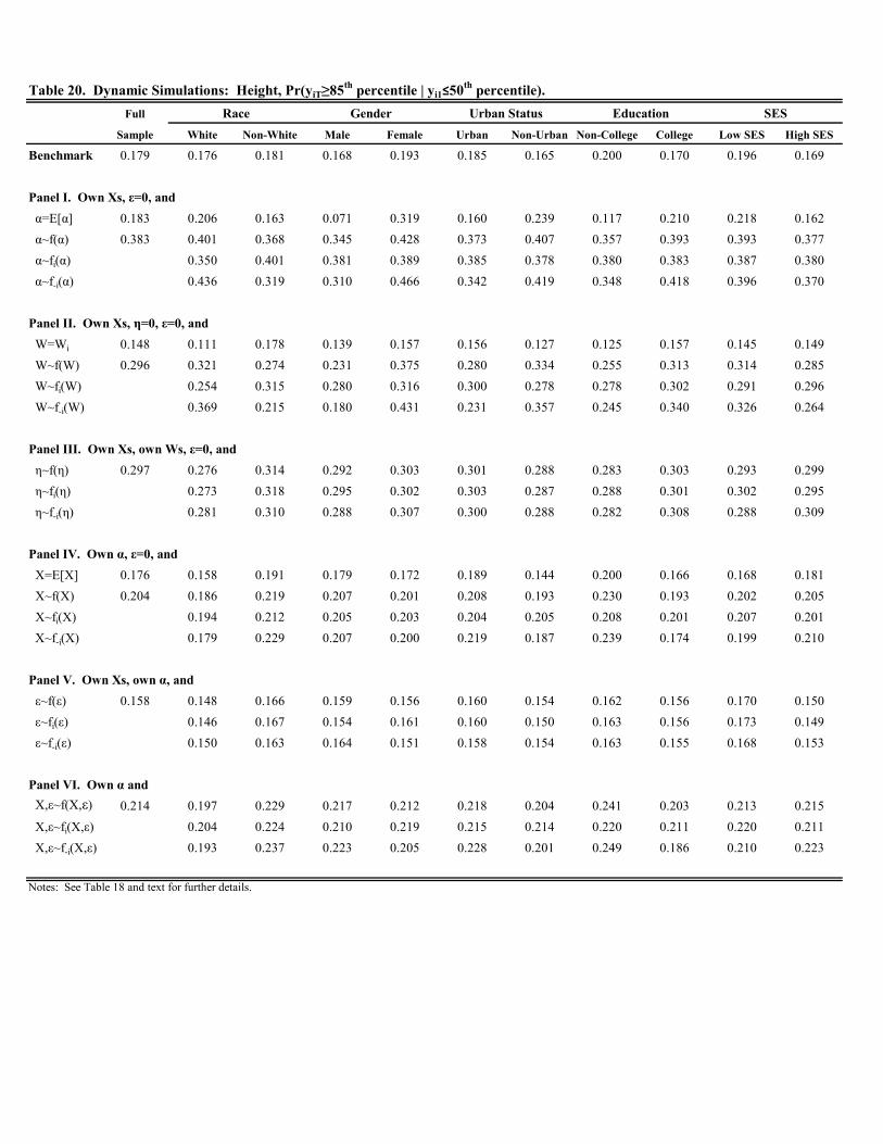
Table 20. Dynamic Simulations: Height, Pr(yiT≥85th percentile | yi1≤50th percentile).Full

Sample White Non-White Male Female Urban Non-Urban Non-College College Low SES High SES

Benchmark 0.179 0.176 0.181 0.168 0.193 0.185 0.165 0.200 0.170 0.196 0.169

Panel I. Own Xs, ε=0, and α=E[α] 0.183 0.206 0.163 0.071 0.319 0.160 0.239 0.117 0.210 0.218 0.162 α~f(α) 0.383 0.401 0.368 0.345 0.428 0.373 0.407 0.357 0.393 0.393 0.377 α~fi(α) 0.350 0.401 0.381 0.389 0.385 0.378 0.380 0.383 0.387 0.380 α~f-i(α) 0.436 0.319 0.310 0.466 0.342 0.419 0.348 0.418 0.396 0.370

Panel II. Own Xs, η=0, ε=0, and W=Wi 0.148 0.111 0.178 0.139 0.157 0.156 0.127 0.125 0.157 0.145 0.149 W~f(W) 0.296 0.321 0.274 0.231 0.375 0.280 0.334 0.255 0.313 0.314 0.285 W~fi(W) 0.254 0.315 0.280 0.316 0.300 0.278 0.278 0.302 0.291 0.296 W~f-i(W) 0.369 0.215 0.180 0.431 0.231 0.357 0.245 0.340 0.326 0.264

Panel III. Own Xs, own Ws, ε=0, and η~f(η) 0.297 0.276 0.314 0.292 0.303 0.301 0.288 0.283 0.303 0.293 0.299 η~fi(η) 0.273 0.318 0.295 0.302 0.303 0.287 0.288 0.301 0.302 0.295 η~f-i(η) 0.281 0.310 0.288 0.307 0.300 0.288 0.282 0.308 0.288 0.309

Panel IV. Own α, ε=0, and X=E[X] 0.176 0.158 0.191 0.179 0.172 0.189 0.144 0.200 0.166 0.168 0.181 X~f(X) 0.204 0.186 0.219 0.207 0.201 0.208 0.193 0.230 0.193 0.202 0.205 X~fi(X) 0.194 0.212 0.205 0.203 0.204 0.205 0.208 0.201 0.207 0.201 X~f-i(X) 0.179 0.229 0.207 0.200 0.219 0.187 0.239 0.174 0.199 0.210

Panel V. Own Xs, own α, and ε~f(ε) 0.158 0.148 0.166 0.159 0.156 0.160 0.154 0.162 0.156 0.170 0.150 ε~fi(ε) 0.146 0.167 0.154 0.161 0.160 0.150 0.163 0.156 0.173 0.149 ε~f-i(ε) 0.150 0.163 0.164 0.151 0.158 0.154 0.163 0.155 0.168 0.153

Panel VI. Own α and X,ε~f(X,ε) 0.214 0.197 0.229 0.217 0.212 0.218 0.204 0.241 0.203 0.213 0.215 X,ε~fi(X,ε) 0.204 0.224 0.210 0.219 0.215 0.214 0.220 0.211 0.220 0.211 X,ε~f-i(X,ε) 0.193 0.237 0.223 0.205 0.228 0.201 0.249 0.186 0.210 0.223

Gender Urban Status Education SES

Notes: See Table 18 and text for further details.

Race