
The Optimal Timing of Unemployment Bene ts: Theory and...
123
The Optimal Timing of Unemployment Benefits: Theory and Evidence from Sweden J Kolsrud Uppsala C Landais LSE P Nilsson IIES J Spinnewijn * LSE September 14, 2017 Abstract This paper provides a simple, yet robust framework to evaluate the time profile of bene- fits paid during an unemployment spell. We derive sufficient-statistics formulae capturing the marginal insurance value and incentive costs of unemployment benefits paid at different times during a spell. Our approach allows us to revisit separate arguments for inclining or declining profiles put forward in the theoretical literature and to identify welfare-improving changes in the benefit profile that account for all relevant arguments jointly. For the empirical implemen- tation, we use administrative data on unemployment, linked to data on consumption, income and wealth in Sweden. First, we exploit duration-dependent kinks in the replacement rate and find that, if anything, the moral hazard cost of benefits is larger when paid earlier in the spell. Second, we find that the drop in consumption affecting the insurance value of benefits is large from the start of the spell, but further increases throughout the spell. In trading off insurance and incentives, our analysis suggests that the flat benefit profile in Sweden has been too gener- ous overall. However, both from the insurance and the incentives side, we find no evidence to support the introduction of a declining tilt in the profile. Keywords: Unemployment, Dynamic Policy, Sufficient Statistics, Consumption Smoothing JEL codes: H20, J64 * We thank Tony Atkinson, Richard Blundell, Raj Chetty, Liran Einav, Hugo Hopenhayn, Philipp Kircher, Henrik Kleven, Alan Manning, Arash Nekoei, Nicola Pavoni, Torsten Persson, Jean-Marc Robin, Emmanuel Saez, Florian Scheuer, Robert Shimer, Frans Spinnewyn, Ivan Werning, Gabriel Zucman and seminar participants at the NBER PF Spring Meeting, SED Warsaw, EEA Mannheim, DIW Berlin, Kiel, Zurich, Helsinki, Stanford, Leuven, Uppsala, IIES, Yale, IFS, Wharton, Sciences Po, UCLA, Sussex, Berkeley, MIT, Columbia, LMU and LSE for helpful discussions and suggestions. We also thank Iain Bamford, Albert Brue-Perez, Jack Fisher, Benjamin Hartung, Panos Mavrokonstantis and Yannick Schindler for excellent research assistance. We acknowledge financial support from the ERC (grant #716485 and #716485), the Sloan foundation (NBER grant #22-2382-15-1-33-003), STICERD and the CEP. 1
Transcript of The Optimal Timing of Unemployment Bene ts: Theory and...

The Optimal Timing of Unemployment Benefits:
Theory and Evidence from Sweden
J Kolsrud
Uppsala
C Landais
LSE
P Nilsson
IIES
J Spinnewijn∗
LSE
September 14, 2017
Abstract
This paper provides a simple, yet robust framework to evaluate the time profile of bene-
fits paid during an unemployment spell. We derive sufficient-statistics formulae capturing the
marginal insurance value and incentive costs of unemployment benefits paid at different times
during a spell. Our approach allows us to revisit separate arguments for inclining or declining
profiles put forward in the theoretical literature and to identify welfare-improving changes in
the benefit profile that account for all relevant arguments jointly. For the empirical implemen-
tation, we use administrative data on unemployment, linked to data on consumption, income
and wealth in Sweden. First, we exploit duration-dependent kinks in the replacement rate and
find that, if anything, the moral hazard cost of benefits is larger when paid earlier in the spell.
Second, we find that the drop in consumption affecting the insurance value of benefits is large
from the start of the spell, but further increases throughout the spell. In trading off insurance
and incentives, our analysis suggests that the flat benefit profile in Sweden has been too gener-
ous overall. However, both from the insurance and the incentives side, we find no evidence to
support the introduction of a declining tilt in the profile.
Keywords: Unemployment, Dynamic Policy, Sufficient Statistics, Consumption Smoothing
JEL codes: H20, J64
∗We thank Tony Atkinson, Richard Blundell, Raj Chetty, Liran Einav, Hugo Hopenhayn, Philipp Kircher, HenrikKleven, Alan Manning, Arash Nekoei, Nicola Pavoni, Torsten Persson, Jean-Marc Robin, Emmanuel Saez, FlorianScheuer, Robert Shimer, Frans Spinnewyn, Ivan Werning, Gabriel Zucman and seminar participants at the NBER PFSpring Meeting, SED Warsaw, EEA Mannheim, DIW Berlin, Kiel, Zurich, Helsinki, Stanford, Leuven, Uppsala, IIES,Yale, IFS, Wharton, Sciences Po, UCLA, Sussex, Berkeley, MIT, Columbia, LMU and LSE for helpful discussions andsuggestions. We also thank Iain Bamford, Albert Brue-Perez, Jack Fisher, Benjamin Hartung, Panos Mavrokonstantisand Yannick Schindler for excellent research assistance. We acknowledge financial support from the ERC (grant#716485 and #716485), the Sloan foundation (NBER grant #22-2382-15-1-33-003), STICERD and the CEP.
1

The key objective of social insurance programs is to provide insurance against adverse events
while maintaining incentives. The impact of these adverse events is dynamic and so are the insur-
ance value and incentive cost of social protection against these events. As a consequence, the design
of social insurance policies tends to be dynamic as well, specifying a schedule of benefits and taxes
that are time-dependent. In the context of unemployment insurance (UI), the UI policy specifies
a full benefit profile designed to balance incentives and insurance throughout the unemployment
spell. Solving this dynamic problem can prove daunting, especially when adding important fea-
tures of unemployment dynamics involving selection and non-stationarities. Indeed, there seems to
be little consensus in practice on the optimal profile of UI benefits. Unemployment policies vary
substantially across countries in the time profile of benefits paid during an unemployment spell,
above and beyond differences in the overall generosity. In the US, benefits are paid only during the
first six months of unemployment. In other countries, like Belgium and Sweden, the unemployed
could receive the same benefit level forever. Recent policy reforms, however, reduced the benefits
for the long-term unemployed relative to the short-term unemployed.
This paper proposes and implements an evidence-based framework to characterize the optimal
time profile of UI benefits and evaluate the welfare consequences of changes in the profile of existing
UI policies. In doing so, this paper aims to bridge three different strands of the literature. There is
an influential theoretical literature on optimal dynamic policies, but derived in stylized models that
are often difficult to connect to the data (e.g. Shavell and Weiss [1979], Hopenhayn and Nicolini
[1997], Werning [2002]). An important empirical literature has analyzed the structural dynamics
of unemployment, but without drawing the consequences for dynamic policies (e.g. Van den Berg
[1990], Eckstein and Van den Berg [2007]). Finally, a recent, but growing empirical literature
started evaluating social insurance design using the so-called sufficient statistics approach, but this
literature has been mostly silent about the dynamic features of social insurance programs (e.g.
Chetty [2008a], Schmieder et al. [2012b]).
In the spirit of the sufficient-statistics approach we derive a characterization of the optimal pro-
file of unemployment benefits based on a limited set of high-level statistics. This simple, yet robust
characterization provides new and transparent insights on the forces affecting the optimal trade-off
between insurance and incentives costs throughout the unemployment spell. Our approach also
identifies the relevant behavioral responses in this dynamic context to evaluate the welfare conse-
quences of (local) changes in the policy. Our analysis therefore provides a clear guide for dynamic
policy design and in particular for analyzing how insurance value and incentive cost of unemploy-
ment benefits evolve over the unemployment spell. We implement this approach empirically, using
Swedish administrative data on unemployment, linked with survey data on consumption and tax
register data on income and wealth.
We start by setting up a rich, dynamic model of unemployment that incorporates job search and
consumption decisions and which allows for unobservable heterogeneity and duration dependence
in job finding rates in addition to unobservable heterogeneity in assets and preferences. Using
dynamic envelope conditions, we show that the Baily-Chetty intuition (Baily [1978], Chetty [2006])
2

generalizes for a dynamic unemployment policy: the UI benefits paid at time t of the unemployment
spell should balance the corresponding insurance value with the implied moral hazard (or incentive)
cost at the margin. At the optimal policy, the marginal value and cost are equalized for any part
of the benefit profile. If they are not, one can identify (local) policy changes that increase welfare.
Like in the original Baily-Chetty formula, the insurance value and moral hazard cost of the dy-
namic policy can be expressed as a function of identifiable and estimable statistics. The incentive
cost of benefits paid at time t of the unemployment spell depends only on the behavioral revenue
effect, i.e., the effect of this benefit level on the government expenditures through agents’ unem-
ployment responses. This fiscal externality is fully captured by the responses of the survival rate
throughout the unemployment spell, weighted by the benefit levels paid. In other words, regardless
of the primitives underlying the dynamics of the agents’ search behavior (e.g., heterogeneity vs.
true duration dependence in exit rates), these survival rate responses are sufficient to evaluate the
incentive cost of changes in the benefit profile. From the insurance perspective, the marginal value
of benefits paid at time t of the unemployment spell depends only on the average marginal utility
of consumption for agents unemployed at time t. To capture this insurance value, we explore the
robustness of the so-called consumption implementation approach, which consists in evaluating the
marginal utility of consumption using observed consumption patterns over the unemployment spell
and calibrated values of risk aversion. We demonstrate how the nature of selection into longer
unemployment spells can affect the relative consumption smoothing gain from benefits paid at
different time t of the unemployment spell.
The empirical part of this paper provides novel insights on the incentive costs and insurance
value of UI benefits over the unemployment spell. We use a unique administrative dataset in Sweden
based on unemployment and tax and asset registers for the universe of Swedish individuals from 1999
until 2007, combined with surveys on household consumption for a subset of the population. We first
exploit duration-dependent caps on unemployment benefits using a regression kink design. These
caps have been affected by several policy reforms, allowing us to estimate non-parametrically how
unemployment survival responds to different variations in the benefit profile. The policy variation
also offers compelling placebo settings that confirm the robustness of our approach. We then
leverage the comprehensive information on income, transfers and wealth from Swedish registers to
construct a residual measure of household expenditures, and, linking this measure to unemployment
records, we identify how consumption expenditures change with unemployment and the duration
of an unemployment spell in particular. We provide complementary and robustness analysis using
survey data on consumption expenditures linked to unemployment records.
Our empirical analysis provides the following main results:
First, unemployment durations respond significantly to changes in benefit levels, whether these
benefits are paid early or later in the spell. Furthermore, we find that the response to changes in
benefits paid earlier in the spell is larger than the response to benefits paid later in the spell. This
result may seem surprising. All else equal, the incentive cost from increasing benefits for the long-
term unemployed is expected to be larger as it also discourages the short-term unemployed from
3

leaving unemployment when they are forward-looking. Using the same regression-kink design, we
do provide clear evidence that exit rates early in the spell respond to benefit changes applying later
in the spell, but also that agents become less responsive to comparable changes in the policy later
in the spell. Importantly, such non-stationary forces, which may be driven by duration dependence
or dynamic selection on returns to search effort over the unemployment spell, are large enough to
offset the significant effect of forward-looking incentives.
Second, consumption expenditures drop substantially and early in the spell. We find that
expenditures drop on average by 4.4% in the first 20 weeks of unemployment, compared to their
pre-unemployment level. This drop deepens to 9.1% on average for those who are unemployed
for longer. We also leverage the richness of the data to document the mechanisms underlying the
observed patterns of consumption, and how they translate into consumption smoothing gains of
UI benefits over the spell. We show that the role of selection effects in explaining the observed
consumption patterns is rather limited. We document the role of assets and liquidity constraints in
explaining the drop in consumption over the spell, and show the limited role of the the added-worker
effect in smoothing the unemployment shock, even for long-term unemployed. The consumption
surveys also shed light on the types of consumption goods that individuals adjust over the spell,
including substitution towards home production and away from durable goods. Taken together,
our evidence consistently indicates that the consumption smoothing value of UI is higher for the
long-term unemployed.
Finally, our empirical estimates can be mapped into the sufficient statistics derived in our
theoretical analysis, allowing for a transparent local evaluation of the benefit levels in a two-
part benefit profile. Our baseline implementation assumes preference homogeneity, separability
between consumption and leisure, and the absence of other externalities (besides the described
fiscal externality). Since we find that in Sweden the incentive costs are high relative to the drop
in consumption throughout the unemployment spell, our implementation suggests that reducing
the generosity of either part of the benefit profile increases welfare for reasonable values of risk
aversion. The incentive cost, however, decreases over the unemployment spell as do the consumption
expenditures of the unemployed. In the absence of offsetting selection on preferences, our estimates
suggest a welfare gain of decreasing the marginal krona spent on the short-term unemployed that
is more than twice as high as decreasing the marginal krona spent on the long-term unemployed.
As the benefit profile was flat during our period of study, this suggests that the introduction of an
inclining benefit profile could have increased welfare. We provide a complementary welfare analysis
based on a structural model. We use our empirical analysis of mechanisms to inform the choice
of primitives of the model, that we then calibrate to match the sufficient statistics underlying our
local policy recommendations. The structural analysis allows us to go beyond these local policy
recommendations, but relies on the structure of the calibrated model. The calibration exercise
indicates that an inclining tilt remains welfare improving when lowering the overall generosity of
the policy.
Our paper contributes to several literatures. First, the sufficient-statistics approach has a long
4

tradition in UI starting with Baily [1978], implemented by Gruber [1997], generalized by Chetty
[2006] and recently reviewed in Chetty and Finkelstein [2013]. To date, this literature has focused
almost entirely on the optimal average generosity of the system.1 Conversely, the theoretical lit-
erature on the optimal time profile of UI has generated results in stationary, representative-agent
models, which are hard to take to the data. Our analysis shows how the previously identified
forces (e.g., in Hopenhayn and Nicolini [1997] and Shimer and Werning [2008]) come together,
but also integrates heterogeneity and duration-dependence (see for example Shimer and Werning
[2006], Pavoni [2009]). Second, our empirical analysis of unemployment responses relates to a long
literature on labor supply effects of social insurance. This literature has focused on exploiting
isolated sources of variation in one part of the benefit profile.2 We contribute by explicitly us-
ing duration-dependent variation in benefits and identifying the welfare-relevant unemployment
responses for multiple parts of the benefit profile. Our analysis indicates that differences in the
timing of the benefit variation could explain different estimates of unemployment responses in the
literature. Finally, a large literature has used consumption surveys to analyze consumption drops
as a response of income shocks and unemployment in particular (e.g., Gruber [1997]). We provide
novel insights on the evolution of consumption as a function of time spent unemployed. We do this
using administrative data on income and wealth to construct a residual, registry-based measure of
consumption, which allows us to identify moral hazard costs and consumption responses for the
very same sample of unemployed.3
The remainder of the paper proceeds as follows. Section 1 analyzes the characterization and im-
plementation of sufficient-statistics formulae for the evaluation of local policy changes in a dynamic
model of unemployment. Section 2 describes our data and the policy context in Sweden. Section
3 describes our regression kink design and provides estimates of the policy-relevant unemployment
elasticities. Section 4 analyzes how consumption evolves during the unemployment spell and how
this translates to the consumption smoothing gains of UI. Section 5 analyzes welfare complementing
the implementation of the sufficient statistics with a calibration exercise of our structural model.
Section 6 concludes.
1 Model
This section sets up a dynamic model of unemployment and identifies the key trade-offs in design-
ing the time profile of the unemployment benefits. We provide a characterization of the optimal
profile in a non-stationary environment with heterogeneous agents. In the spirit of the “sufficient-
statistics” literature, our approach consists in identifying the minimal level of information necessary
1Recent dynamic extensions of the Baily-Chetty formula can be found in Schmieder et al. [2012b], analyzing thepotential benefit duration for a given benefit level, and in Spinnewijn [2015], providing a formula for the optimalintercept and slope of a linear benefit profile.
2See Krueger and Meyer [2002] for a review on the labor supply effects of social insurance. Recent examplesanalyzing variation in UI are Rothstein [2011], Valletta and Farber [2011], Landais [2015], Card et al. [2015] and Masand Jonhston [2015].
3See for instance Mogstad and Kostol [2015], Kreiner et al. [2014] and Pistaferri [2015] for a survey of recentdevelopments of consumption analysis using registry data.
5
for this characterization. Our focus goes beyond the primitives of the environment and the assump-
tions on agents’ behavior in our specific model. Instead, we aim to identify the observable variables
that are relevant for policy in a broad class of models and can be estimated empirically.
1.1 Setup
We first describe the set up of our dynamic unemployment model, building on the dynamic model
in Chetty [2006], the agents’ choices and the unemployment policy. We try to save on notation
in the main text, but provide more details in the technical Appendix A. We consider a partial
equilibrium framework with a continuum of agents with mass 1. The model is in discrete time t,
starts at t = 1 and ends at t = T .
Each agent i starts unemployed and remains unemployed until she finds work. Once an agent
has found work, she remains employed until the end. When employed, the agent earns w, when un-
employed she earns 0. Before the start of the model, the government commits to an unemployment
policy P providing insurance against the unemployment risk: the policy specifies an unemployment
benefit profile depending on the duration of the ongoing unemployment spell (i.e., a benefit level bt
for each time t if the unemployment spell is still ongoing) and a uniform tax τ paid when employed.
Job search Each agent i decides at each time t how much search effort si,t to exert as long
as she is unemployed. This effort level determines the agent’s exit probability at time t. We
denote the agent’s exit rate out of unemployment at time t by hi,t (si,t). We allow this mapping
to depend on the type of agent i, capturing heterogeneity in employability across agents, and the
time t she has spent unemployed, capturing differences in employment prospects due to the time
spent unemployed.4 The agent’s probability to be unemployed after t periods equals the survival
probability Si,t ≡∏t−1t′=1(1− hi,t′
(si,t′)) with Si,1 = 1. While we cannot observe an agent’s specific
survival probability, we can observe the population average of survival probabilities St ≡∫Si,tdi.
Intertemporal Consumption Each agent i decides at each time t how much to borrow
or save (at interest rate r). An agent starts the unemployment spell with asset level ai,1, but
borrowing constraints prevent her from running down her asset below ai at any time. The agent’s
savings decisions determine her consumption level throughout the unemployment spell and when re-
employed. We denote these levels by cui,t and cei,t for when unemployed and employed respectively.5
While we cannot observe an agent’s contingent consumption plan, we can observe average levels of
consumption, for example at different spell lengths, cut =∫
(Si,t/St)cui,tdi.
4Potential reasons for true duration-dependence in exit rates are human capital depreciation (see Acemoglu [1995]and Ljungqvist and Sargent [1998a]) and stock-flow sampling (see Coles and Smith [1998]). We assume exogenousexit rate functions that only depend on the agent’s search, but do not directly depend on other job seekers’ searchlike in rationing models (e.g., Michaillat [2012b]) or on the unemployment policy like in employer screening models(e.g., Lockwood [1991]). We discuss this further in Section 1.4 and Appendix Section A.2.
5The agent’s consumption choice at time t will depend on her unemployment history. In particular, even when em-ployed, the agent’s unemployment history will have affected her asset accumulation and thus her optimal consumptionat time t. We introduce formal notation to denote the relevant state variables in the technical appendix.
6

Preferences Each agent i has time-separable preferences (with discount factor β) with per-
period utility increasing in consumption, but decreasing in search efforts exerted when unemployed.
We denote agent i’s per-period utility by vui (cui,t, si,t) and vei (cei,t). We allow for preference hetero-
geneity and non-separable preferences in the characterization of the optimal policy, but will assume
preference homogeneity and separability between consumption and efforts in our baseline imple-
mentation. Each agent chooses how much to search and how much to consume in order to maximize
her expected utility, taking the unemployment policy P as given. The dynamics of the agent’s be-
havior depend on her assets and the time spent unemployed in addition to the unemployment policy.
To reduce notation, we will drop the arguments of the agent’s behavior. We denote the agent’s
value function of her maximization problem by Vi (P ), accounting for her optimal consumption and
search choices and potentially binding borrowing constraints.
Unemployment Policy We characterize the welfare impact of local deviations from the
unemployment policy P. In particular, we consider changes in the benefit bt paid at time t of the
unemployment spell, starting from any benefit profile btTt=1. Our expressions naturally generalize
for changes in step-wise policies, paying benefit level bk for part k) of the unemployment spell (from
time Bk−1 until Bk. Flat benefit profiles with no or few steps are very common in practice. In
Sweden, the unemployment policy in Sweden is entirely flat for some workers and exists of two parts
for other, with the benefit dropping to a lower (positive) level at twenty weeks of unemployment.6
Our implementation evaluates the benefit levels of this two-tier benefit profile.
The government’s budget depends on the expected benefit payments paid to the unemployed
and the expected tax revenues received from the employed. Note that the average unemployment
duration D simply equals the sum of the survival rates at each duration∑T
t=1 St. Similarly, Dk =
ΣBkBk−1+1St denotes the expected time spent unemployed while receiving benefit bk, which we refer
to as the average benefit duration. We ignore time discounting in our characterization of the optimal
policy (i.e., 1 + r = β = 1), but generalize this in the technical Appendix A.
The government’s budget simplifies to
G (P ) = [T −D]τ − ΣTt=1Stbt. (1)
Social welfare associated with an unemployment policy P can be written as the Lagrangian
W (P ) =
∫Vi (P ) di+ λ
[G (P )− G
], (2)
where λ equals the Lagrange multiplier on the government’s budget constraint and G is an exoge-
nous revenue constraint. We assume that the social welfare function is differentiable.
6We discuss the details of the Swedish unemployment policy in Section 2.1.
7

1.2 Dynamic Sufficient Statistics
We consider the welfare impact of local policy deviations, which we decompose into the corre-
sponding consumption smoothing gains and moral hazard cost. Our approach does not provide an
explicit characterization of the optimal policy, but is sufficient to test for the (local) optimality of
the policy in place. Evaluating local policy changes, away from the optimal policy, is of interest
to identify how welfare can be increased and how the policy can be changed towards the optimal
policy (if welfare is concave in the policy variables).
Consider now an increase in the benefit level bt in period t of the unemployment spell. The
total impact on welfare depends on how much the unemployed value this increase in benefits bt
relative to its budgetary cost,
∂W (P )
∂bt=
∫∂Vi (P )
∂btdi+ λ
∂G (P )
∂bt. (3)
This welfare effect depends on the agents’ behavioral responses to the policy, but only to the extent
that the agents’ behavior has consequences that they did not internalize themselves. Indeed, an
agent’s response to a policy change will have only a second order impact on her own welfare Vi (P ).
Assuming differentiability, this follows from the envelope conditions ∂Vi/∂xzi,t′ = 0, which hold for
any behavior xzi,t′ the agent optimizes over, at any time t′, when employed (z = e) or unemployed
(z = u) and when the borrowing constraint is binding or not (see Chetty [2006]).7 So we only need
to account for the impact of behavioral responses on the government’s budget G (P ) and the direct
impact of the policy change on agents’ welfare, which proves particularly powerful in this dynamic
context.
Moral Hazard Consider first the budgetary impact from an increase in bt. The first effect
from increasing the benefit level is mechanical and depends on the share of workers still unemployed
after t periods, St. The second effect is behavioral and is determined by the budgetary cost of the
agents’ reduced search in response to the more generous benefit. This depends on the induced
change in the average survival rates throughout the unemployment spell,
∂G (P )
∂bt= −St − ΣT
t′=1
∂St′
∂bt(bt′ + τ) = −St ×
[1 + ΣT
t′=1
St′ (bt′ + τ)
Stbtεt′,t
](4)
≡ −St × [1 +MHt] . (5)
The moral hazard cost MHt of an increase in bt simply equals the weighted sum of the elasticities
εt′,t = (∂St′/∂bt) / (St′/bt) of the average survival rate St′ with respect to the benefit level bt. The
elasticities are weighted by the relative share of the budget spent at different times during the
unemployment spell. The budgetary spillover effects of a change in bt on other parts of the policy
7Changes in the choice variables might be discontinuous in response to small policy changes. In principle wecan allow for such discontinuous behavioral responses if they average out when integrating across heterogeneousindividuals so that the social welfare function is differentiable.
8

is less relevant the less generous these other parts are. There is, however, a correction for the tax
rate because more time spent unemployed also reduces the taxes received from employment.
Evaluated at a flat profile (bt = b for all t), the moral hazard cost of an increase at time t is
fully determined by the response in the average duration D, scaled by the survival rate at t,
MHt =∂D/∂btSt
(b+ τ
)=D(b+ τ
)Stb
εD,bt . (6)
This average duration response combines the potentially heterogeneous responses by unemployed
workers throughout the unemployment spell, including responses earlier in the spell in anticipation
of the increase in bt and selection effects later in the spell due to the increase in bt.
Consumption Smoothing Let us now turn to the insurance value of an increase in the
benefit bt. Due to the envelope conditions, the welfare increase is completely captured by the
marginal utility of consumption at this time of the spell for the agents who are still unemployed,
∫∂Vi (P )
∂btdi =
∫Si,t
∂vui
(cui,t, si,t
)∂cui,t
di,
≡ St × Eut
∂vui(cui,t, si,t
)∂cui,t
.
As defined above, the expectation operator Eut takes the weighted average over all individuals’
marginal utility of consumption in the t-th period of the unemployment spell (with weights Si,t/St).
By analogy to the budgetary cost, we can write∫∂Vi (P )
∂btdi/λ = St × [1 + CSt] , (7)
where the consumption smoothing gain CSt ≡ Eut[∂vui (cui,t,si,t)
∂cui,t
]− λ/λ. Since the Lagrange mul-
tiplier λ equals the shadow cost of the government’s budget constraint, the consumption smoothing
gains can be interpreted as the return of a government dollar spent to the unemployed in period t of
the unemployment spell relative to the value of an unconditional transfer.8 Importantly, in spite of
potential heterogeneity across agents and in their responses to the policy change, the welfare gain
is fully captured by the average marginal utility of consumption at time t of the unemployment
spell.
Welfare Impact An optimal unemployment policy balances consumption smoothing gains
and moral hazard costs. A dynamic benefit profile allows solving this trade-off at each point during
8Note that when the government can provide such lump sum transfer, it would be optimally set such that λ equalsthe average marginal value of resources at the start of this model. More generally, the consumption smoothing gainCSt corresponds to the net social marginal welfare weight assigned to the unemployed at time t.
9

the unemployment spell. Combining expressions (3), (5) and (7), we find
∂W (P )
∂bt= λSt × [CSt −MHt] .
An increase (decrease) in benefit bt increases welfare as long as the consumption smoothing gains
are larger (smaller) than the moral hazard cost. This implies a natural characterization of the
optimal policy:
Proposition 1. Consider an unemployment policy P , charging tax τ to the employed and paying a
dynamic benefit profile btTt=1 to the unemployed. Assuming differentiability, an interior, optimal
policy needs to satisfy
Eut
[∂vui (cui,t,si,t)
∂cui,t
]− λ
λ= ΣT
t′=1
St′ (bt′ + τ)
Stbt× εt′,t for each t, (8)
λ− Ee[∂vei (cei,t)∂cei,t
]λ
= ΣTt′=1
St′ (bt′ + τ)
(T −D) τ× εt′,τ , (9)
and the budget constraint G (P ) = G.
Proof. See Appendix A.
The expectation operator Eut is defined as before and takes the weighted average over all in-
dividuals unemployed at time t (with weights Si,t/St). Similarly, Ee takes the weighted average
over all individuals and times in employment (with weights (1− Si,t) / [T −D]). The conditions
for all benefit levels and the tax level in Proposition 1 can be combined to recover the well-known
Baily-Chetty formula (Baily [1978] and Chetty [2006]) for a flat benefit profile (bt = b),9
Eu[∂vui (cui,t,si,t)
∂cui,t]− Ee[∂v
ei (cei,t)∂cei,t
]
Ee[∂vei (cei,t)∂cei,t
]
∼=b+ τ
bεD,b. (10)
Our analysis extends the “sufficient statistics” approach to the dynamics of the unemployment
policy, aiming to provide a simple, yet robust guide for dynamic policy design. As we argue below,
the characterization depends on a limited set of empirically implementable moments and is robust
to the primitives and specific assumptions of the underlying model. Our dynamic extension also
overcomes challenges that have constrained empirical and theoretical work in identifying the key
dynamic forces. Empirically, identifying the role of different, non-stationary forces underlying a
9The expectation operator Eu in condition (10) takes the weighted average over all unemployment periods (withweights Si,t/D). The approximation relies on the unemployment response to taxes to be small. The exact expressionfor the right-hand side is [1 + b+τ
bεD,b]/[1 + b+τ
τεT−D,τ ]− 1. Note that the standard Baily-Chetty formulation uses
the elasticity wrt a budget-balanced increase in the benefit level, joint with an increase in the tax level, and ignoresother tax distortions in the economy. Our model allows the tax to cover general expenditures G and our expressionsare in terms of partial elasticities, which are more transparent for multi-dimensional policies and correspond moredirectly to the policy variation we exploit in the empirical analysis.
10

job seeker’s environment, including the role of unobserved heterogeneity, proves daunting. Several
studies have tried to estimate or calibrate the contribution to the negative duration-dependence of
exit rates from dynamic selection effects, true duration-dependence in the search environment (e.g.,
skill-depreciation or stock-flow sampling of vacancies), or an interaction of the two (e.g., duration-
based employer screening).10 Theoretically, it has also proven difficult to derive the optimal benefit
profile and, in particular, the impact of non-stationary forces and heterogeneity (see Shimer and
Werning [2006], Pavoni [2009]). In contrast, Proposition 1 provides a robust mapping from a non-
stationary model with heterogeneous agents into a set of implementable moments to evaluate the
benefit profile.11
1.3 Implementation
We first consider the implementability of our characterization, which guides our empirical analysis
in Sections 3 and 4. Our focus is on the benefit levels of a two-part policy (b1, b2, B) paying benefit
b1 until time B and b2 thereafter, like in place in Sweden (see Section 2.1) and illustrated in Panels
A.I and B.I of Figure 1. This section clarifies additional assumptions and the policy variation
required for the implementation we propose.
Moral hazard cost An extensive literature has analyzed unemployment responses to changes
in the unemployment policy. Our analysis indicates that it is essential to have variation in unem-
ployment benefits at different times during the unemployment spell.
For a two-part profile, the benefit duration D1 (D2), which denotes the expected time spent
receiving benefit b1 (b2), corresponds to the area under the survival function before (after) B, as
illustrated in Panels A.II and B.II. The moral hazard cost of changing the benefit level bk during
part k of the policy fully depends on the response in both benefit durations,
MH1 =b1 + τ
b1εD1,b1 +
D2 (b2 + τ)
D1b1εD2,b1 (11)
MH2 =D1 (b1 + τ)
D2b2εD1,b2 +
b2 + τ
b2εD2,b2 (12)
Panel A and Panel B of Figure 1 illustrate how estimating the moral hazard costs requires
duration-dependent policy variation. Rather than having benefits change throughout the spell,
which would be sufficient to evaluate a flat policy, we need changes in benefits paid only to the
short-term db1 or to the long-term unemployed db2.
Our evaluation of the benefit profile is conditional on B, which determines the potential duration
of the two parts. Still, our expressions can be used to approximate the moral hazard cost of changing
the potential benefit durations, as analyzed in Schmieder et al. [2012b]. Indeed, an increase in
10See Ljungqvist and Sargent [1998a] and Machin and Manning [1999] for reviews on the negative duration depen-dence of exit rates out of unemployment. See Kroft et al. [2013] and Alvarez et al. [2016] for recent examples.
11In Section 5.2, we also show how this mapping can be useful to uncover the role of stationary vs. non-stationaryforces from the estimated moments and understand their respective role for the optimal timing of benefits.
11

potential benefit duration from B to B + 1 corresponds to a (discrete) change of benefit bB+1 at
B+1 (from level b2 to level b1), where the moral hazard cost of a (marginal) change in bB+1 equals
MHbB+1=∂D1/∂bB+1
SB+1(b1 + τ) +
∂D2/∂bB+1
SB+1(b2 + τ) .
While there is no such policy variation in the Swedish context, Schmieder and Von Wachter [2016]
review recent empirical work that analyzes either duration responses in unemployment or UI benefit
receipt to changes in potential benefit duration. The expression above shows that the responses
in both the benefit duration D1 and the average duration D (since D2 = D − D1) affect the
fiscal externality, unless the tax is small (τ ∼= 0) and no benefits are paid after time B (b2 = 0).
Importantly, any evaluation of the potential benefit duration would be conditional on the benefit
levels and does not allow to evaluate the tilt of the profile itself.
Consumption Smoothing Attempts at quantifying the consumption smoothing gains of
UI policies have been more scarce as the estimation of differences in marginal utility levels proves
difficult in practice. We follow the “consumption implementation” approach (Gruber [1997], Chetty
[2006]), relating the difference in marginal utilities to the difference in consumption levels, and
extend this approach to our dynamic setting. Using consumption wedges to actually quantify the
relevant consumption smoothing gains of UI requires the following assumptions:12
First, we rely on approximations of the marginal utility of consumption using Taylor expansions,
assuming that third- and higher-order derivatives of the utility function are small. That is,
∂vui∂c
(cui,t, si,t
) ∼= ∂vui∂c
(c, si,t)×[1− γi,t ×
c− cui,tc
],
where γi,t ≡ c∂2vui∂c2
(c, si,t) /∂vui∂c (c, si,t) equals the relative risk aversion.13
Second, we assume that preferences over consumption are separable from leisure, i.e., ∂vui (c, s) /∂c =
∂vei (c) /∂c = v′i (c), so that consumption smoothing benefits do not depend on other behavior or the
employment status itself, but only on the consumption wedges. This excludes potentially important
complementarities between consumption and leisure during unemployment.14
Third, we express the consumption smoothing gains from an increase in unemployment benefits
relative to an increase in resources just before the onset of the unemployment spell (denoted by
12Note that the limitations of the consumption-based implementation have inspired alternative approaches relatingthe marginal utility gap to observable behavioral responses: Chetty [2008a] decomposes unemployment responses inliquidity and substitution effects, Shimer and Werning [2007] analyze reservation wage responses. The extension ofthese alternative approaches to a dynamic setting seems promising, but requires that the policy variation used forthe static implementation also changes over the unemployment spell.
13If the third-order derivative of the utility function is non-negligible, the consumption smoothing gains dependon an additional term that depends on the coefficient of relative prudence, corresponding to precautionary savingmotives (see Chetty [2006]). We calculate the magnitude of this approximation error in section 5.3.
14In subsection 4.2, we discuss the issues related to this assumption in more detail. One example is the substitutiontowards home production when no longer employed (e.g., Aguiar and Hurst [2005]).
12

v′i (ci,0)). This normalization emphasizes the insurance value of the policy.15
Fourth, we assume that preferences are homogeneous (i.e., vi (c) = v (c)), but we consider the
implications of preference-based selection over the unemployment spell in Section 5.2.
Under these four assumptions, we can approximate the consumption smoothing gains by16
CSk =
1Dk
∫ΣBkBk−1+1Si,tv
′(cui,t
)di−
∫v′ (ci,0) di∫
v′ (ci,0) di(13)
∼=v′ (cuk)− v′ (c0)
v′ (c0)∼= −
v′′ (c0) c0
v′ (c0)×c0 − cukc0
, (14)
where c0 and cuk denote the average consumption level before the onset of the spell and during part
k of the spell. The resulting expression directly relates to the original approximation in Baily [1978]
and highlights the role of the profile of the average consumption level over the unemployment spell
to evaluate the unemployment benefit profile. If the unemployed consume less the longer they are
unemployed, ceteris paribus, unemployment benefits are more valuable later in the spell.
For a two-part profile, the implementation thus comes down to calculating the average wedge in
consumption for the short-term unemployed and the long-term unemployed, as illustrated in Panel
C of Figure 1. Importantly, no policy variation is needed to estimate these consumption wedges.
1.4 Robustness
We briefly consider the robustness of our sufficient-statistics characterization in a dynamic context.
As argued before by Chetty [2006], the set of moments in Proposition 1 are sufficient to provide
local evaluations of the unemployment policy, independently of the underlying primitives. That
is, when different values for our models’ parameters map into the same values for the identified
moments for a given policy, the local policy recommendations remain the same. In particular,
our dynamic model explicitly allows for (exogenous) heterogeneity in exit rate functions across
agents (hi,t (·) 6= hj,t (·)) and variation in exit rates over the unemployment spell (hi,t (·) 6= hi,t′ (·)).While separating unobserved heterogeneity and true duration-dependence in exit rates is hard, our
approach shows that this is unnecessary for estimating the moral hazard cost and its evolution over
15In our stylized model, all individuals start unemployed, so the Lagrange multiplier (evaluated at the optimalpolicy) equals λ =
∫∂V/∂ai,1di =
∫∂V/∂b1di. In Appendix Section A.2.4, we consider a more general model
where agents can start employed or unemployed and may experience multiple spells. The Lagrange multiplier thencorresponds to the average marginal utility of consumption at the start of the model across all individuals. Byconsidering the marginal utility of consumption before the onset of the unemployment spell in our implementation,we are capturing the insurance value of the unemployment policy, while ignoring the value of redistributing betweendifferent types of workers who face different layoff risks. Importantly, the evaluation of (budget-balanced) changes inthe benefit profile is independent of this normalization.
16The first approximation relies on a Taylor expansion of v′(cui,t)
for each individual i and time t around the
average consumption level during the corresponding part k of the unemployment spell, cuk ≡ 1Dk
∫ΣBkBk−1+1c
ui,tSi,tdi,
using1
Dk
∫ΣBkBk−1
Si,tv′′ (cuk)
[cui,t − cut
]di = 0.
This also applies at time t = 0, just before the onset of the unemployment spell. The second approximation simplyuses a Taylor expansion of v′ (cuk) around c0.
13
the unemployment spell. The intuition is that only the survival responses need to be known, as
they fully determine the fiscal externality of job seekers’ behavior. As is well known, this result
criticially relies on the application of the envelope conditions for the job seekers’ behavior (see
Chetty [2006], Chetty and Finkelstein [2013]). The result also indicates that the foundations of
our dynamic model of search and consumption can be further extended without (substantially)
changing the characterization of the optimal benefit profile. That is, the same set of moments
will continue to determine the local evaluation of the unemployment policy.17 Our baseline setup
illustrates this robustness explicitly for exogenous heterogeneity across agents and across durations,
but the intuition generalizes to other models of search and self-insurance.18
While our implementation is robust to heterogeneity in employment prospects and assets and
the corresponding dynamic selection, our baseline implementation assumes preferences that are
homogenous and separable in consumption and search efforts. Under this assumption the relative
consumption smoothing gains, for example for short-term and long-term unemployed, simplify to
the corresponding relative consumption drops, which thus become sufficient to recommend welfare-
improving changes in the tilt of the benefit profile. This avoids the well-known challenge for the
consumption-based implementation of translating consumption wedges to welfare (see Chetty and
Finkelstein [2013]).19 We assess this challenging conversion from consumption into welfare in more
depth and also gauge the potential for dynamic selection on preferences in Sections 4.2 and 5.2.20
Finally, as our characterization critically relies on the application of the envelope theorem, by
the same token, the presence of other externalities – not internalized by agents, but relevant for
welfare – would affect the optimal policy characterization. Recent work has analyzed the impact of
different types of externalities on the characterization of a static unemployment policy.21,22 These
17Chetty [2006] has shown how the simple formula (10) characterizing the flat benefit profile continues to applywith leisure benefits from non-employment, alternative means of self-insurance, spousal labor supply, human capitaldecisions, etc. See the review chapter by Chetty and Finkelstein [2013] for a more detailed discussion of differentadvantages and challenges for the sufficient-statistics approach.
18In Appendix Section A.2.2 we show how our model can be indeed extended to multiple unemployment spells,allowing for moral hazard on the job and different means of self-insurance, while the same formulae continue to apply.The relevant variables for evaluating the benefit profile are the overall unemployment rate and the survival rates St atdifferent unemployment durations, averaged over multiple spells. Layoff responses to UI policy affect the magnitudeof the policy-relevant elasticities, but only if moral hazard on-the-job were to be important. In Appendices A and B,we provide and discuss evidence based on the pdf of pre-unemployment wages around a kink in the unemploymentpolicy that indicates that layoff rates do not respond strongly to the unemployment policy in our empirical context.
19See Chetty [2008a], or Landais [2015], for the development of alternative methods, exploiting comparative staticsof effort choices, in order to to evaluate consumption smoothing gains. These methods could circumvent the issue ofhaving to make assumptions regarding dynamic selection on risk preferences.
20Note also that our model assumes a utilitarian social welfare function. See Andrews and Miller [2013] for adiscussion on the aggregation of individual welfare gains under preference heterogeneity in the context of the Baily-Chetty formula. With heterogeneous Pareto weights, the dynamic selection based on these weights will matter aswell.
21For example, Nekoei and Weber [2015], account for the fiscal impact of reservation wage responses, conditionalon unemployment duration, which tend to be small relative to the duration responses themselves. Spinnewijn [2015]accounts for internalities due to biased beliefs about employment prospects. Landais et al. [2010] adjust the charac-terization to account for frictions in the labor market and general equilibrium effects.
22In Appendix Section A.2.4, we show how our framework can account for the fiscal externality created by thepresence of an income tax used to fund other government expenditures, which we use to analyze the sensitivity ofour welfare recommendations.
14

insights generalize in our dynamic setting, but are of particular relevance for our analysis when
the externality depends on the timing of the unemployment benefits. In Appendix Section A.2,
we demonstrate this in the context of employer screening (e.g., Lockwood [1991]), which gives
rise to negative duration-dependence when employers use unemployment spell length as a negative
signal of unobserved productivity. In such a setting, job seekers do not internalize their impact on
the hiring probability for other job seekers, which happens through the relative survival rates of
different types. As shown by Lehr [2017] for a flat benefit profile, the unemployment policy can
affect this hiring externality, but only if the relative survival rate of different productivity types
depends on the unemployment policy. We show in appendix that for a dynamic benefit profile, the
externality-adjusted moral hazard cost equals
MHxt ≡ ΣT
t′=1
St′
St
[bt′ + τ
btεt′,t − Eut′
(ωht′
∂ht′
∂bt
)], (15)
where ωht′ corresponds to an agent’s welfare gain of finding a job at time t′ and ∂ht′/∂bt equals the
change in the job finding rate due to the employer’s hiring response. If the hiring response depends
on the timing of the benefits, the externality-adjustment could vary over the spell. This requires
the relative survival rate of different productivity types to change with the timing of benefits. In
appendix we demonstrate that types with higher returns to search are more responsive to changes
in benefits early on, but due to their low survival into longer unemployment spells, can be less
responsive to changes in benefits later on. Hence, when types with higher returns to search are
also more productive, the hiring externality can be positive for benefits paid early in the spell, but
negative for benefits paid late in the spell.
2 Context and Data
To implement our formulae and evaluate the profile of UI benefits, two pieces of empirical evidence
are needed. First, one needs to identify and estimate responses of unemployment durations to
variations in the benefit profile, i.e., variations in UI benefits at different points of an unemployment
spell. Second, one needs to estimate the time profile of consumption to identify how consumption
(relative to employment) drops over an unemployment spell.
Our empirical analysis offers contributions on both dimensions by using a unique administrative
dataset that we created in Sweden merging unemployment registers, tax registers - with exhaustive
information on income and wealth - and household consumption surveys. We present here the
institutional background and data used in our empirical implementation.
2.1 Institutional background
In Sweden, displaced workers who have worked for at least 6 months prior to being laid-off are
eligible to unemployment benefits, replacing 80% of their earnings up to a cap. In practice, the level
of the cap is quite low relative to the earnings distribution and applies to about 50% of unemployed
15

workers. Individuals can receive unemployment benefits indefinitely. To continue receiving benefits
after 60 weeks of unemployment, the unemployed must accept to participate in counselling activities
and, potentially, active labor market programs set up by the Public Employment Service. Like in
other Scandinavian countries, UI in Sweden is administered by different unemployment funds (of
which most are affiliated with a labor union) and contributions to the funds are voluntary in
principle. Over the period 1999 to 2007, more than 85% of all workers were contributing to an
unemployment fund. Our sample focuses on workers with more than 6 months of employment
history prior to being laid-off and who contribute to UI funds.
The time profile of benefits has changed during the period we study. Before 2001, the time
profile of UI benefits was flat for all unemployed workers.23 Full-time workers would get daily
benefits of 80% of their pre-unemployment daily wage throughout the spell (i.e., for as long as they
remain unemployed), with daily benefits capped at 580SEK a day (≈ 63USD a day, or 320USD a
week).24 The cap thus applies for daily wages above 725SEK (≈ 399USD a week).25 In July 2001,
a system of duration-dependent caps was introduced, which created a decreasing time profile of
benefits for the unemployed above the threshold wage. The cap for the benefits received during the
first 20 weeks of unemployment was increased to 680SEK (daily wage above 850SEK ≈ 467.5USD
a week) while the cap for benefits received after the first 20 weeks was kept unchanged at 580SEK.
In July 2002, the cap for benefits received during the first 20 weeks of unemployment was increased
to 730SEK (daily wage above 912.5SEK ≈ 500USD a week) and the cap for benefits received after
the first 20 weeks was increased to 680SEK.26
The 2001 and 2002 reforms introduce variation in the benefit profile which makes it possible
to estimate the causal impact of benefits received at different times during the unemployment
spell on survival in unemployment. We explain in Section 3 how the 2001 and 2002 variations
in the duration-dependent caps can be used in a regression kink design to identify the effects on
unemployment durations of UI benefits given in the first 20 weeks of a spell and of benefits given
after 20 weeks.
2.2 Data
Unemployment history data come from the HANDEL register of the Public Employment Service
(PES, Arbetsformedlingen) and were merged with the ASTAT register from the UI administration
(IAF, Inspektionen for Arbetsloshetsforsakringen) in Sweden. The data contain information from
1999 to 2007 on the date the unemployed registered with the PES (which is a pre-requisite to start
23The potential duration of benefits is theoretically infinite in Sweden during our period of interest, and there isno exhaustion point of UI benefits.
24We use the following exchange rate: 1SEK ≈ 0.11USD.25The daily wage is computed as gross monthly earnings divided by number of days worked in the last month prior
to becoming unemployed.26Some unions have launched their own complementary UI-schemes which further increased the cap (by up to 3
times the cap on regular UI) by topping up the regular UI-benefit to 80 percent of the previous wage. Importantly,our regression-kink design analysis focuses on the effect of the 725SEK-kink in the UI schedule, which was removedin 2002 before the introduction of the top-ups, so that all unemployed had to comply to the same kinked schedule ofbenefits.
16

receiving UI benefits), eligibility to receive UI benefits, earnings used to determine UI benefits,
weekly information on benefits received, unemployment status and participation in labor market
programs. We define unemployment as a spell of non-employment, following an involuntary job
loss, and during which an individual has zero earnings, receives unemployment benefits and reports
searching for a full time job.27 To define the start date of an unemployment spell, we use the
registration date at the PES. The end of a spell is defined as finding any employment (part-time or
full-time employment, entering a PES program with subsidized work or training, etc.) or leaving
the PES (labor force exit, exit to another social insurance program such as disability insurance,
etc.).28
These data are linked with the longitudinal dataset LISA which merges several administrative
and tax registers for the universe of Swedish individuals aged 16 and above. In addition to socio-
demographic information (such as age, family situation, education, county of residence, etc.), LISA
contains exhaustive information on earnings, taxes and transfer and capital income on an annual
basis. Data on wealth comes from the wealth tax register (Formogenhetsregistret), which covers
the asset portfolios for the universe of Swedish individuals from 1999 to 2007. The register contains
detailed information on the stock of all financial assets (including debt) and real assets as of
December of each year.29 For the financial assets, we have information on all savings by asset class
(bank accounts, bonds, stocks, mutual funds, private retirement accounts, etc.). The dataset also
contains information on total outstanding debt including mortgage debt, consumer credit, student
debt, etc. For real estate, we have information on all asset holdings at market value as used for
the wealth tax assessment.30 Data on asset balances as of December is complemented with data on
financial asset transactions (KURU) and real estate transactions from the housing registries. The
comprehensiveness and detailed nature of both the income and wealth data in Sweden is exceptional,
providing a unique opportunity to investigate what means individuals use to smooth consumption
(transfers, asset rebalancing, increase in debt, etc.). We take advantage of the richness of the
income and wealth data to construct a registry-based measure of annual household consumption
expenditures as of December of each year. Our approach builds on previous attempts to measure
consumption from registry-data (e.g. Koijen et al. [2014], Browning and Leth-Petersen [2003]) and
is closely related to Eika et al. [2017] in exploiting additional information on asset portfolio choices
and returns to reduce measurement error and excess dispersion of consumption measures based
solely on first-differencing asset stocks. All details regarding the construction of the registry-based
27Involuntary job loss is defined as a layoff or a quit following a “valid reason”. “Valid reasons” for quitting a jobare defined as being sick or injured from working, being bullied at work, or not being paid out one’s wage by one’semployer. Quits are reviewed by the Public Employment Service at the moment an individual registers a new spelland if the quit is made because of a “valid reason”, the individual is eligible for UI and a notification is made in thePES data, allowing us to observe such “quits under valid reasons”. Note however that quits are a small fractions ofspells in our sample: 95.0% of job separations observed in our data are due to layoffs.
28To deal with a few observations without any end date, we censor the duration of spells at two years.29All financial institutions are compelled to report this information directly to the tax administration for the
purpose of the wealth tax, which ensures quality and exhaustiveness of the data. The wealth tax was abolished inSweden in 2007, after which the government collected only limited information on the stock of assets.
30All asset holdings are reported to the tax administration at the individual level. We aggregated assets at thehousehold level using household identifiers from the registry data.
17

measure of consumption are given in Appendix C.1.
The richness of the Swedish administrative data, its universal coverage and panel structure,
enable us to identify duration responses and within-household consumption responses to unem-
ployment shocks for the very same sample of individuals, and with a unique degree of precision. An
important characteristic of the registry-based measure of consumption though, is that it captures
the sum of annual consumption expenditures as of December of each year. While this peculiarity
does not represent a serious limitation to identify higher frequency flows of consumption throughout
the unemployment spell, as shown in section 4, we complement our data with information on con-
sumption available through the yearly household budget survey (HUT, Hushallens utgifter), which
provides direct measures of bi-weekly consumption expenditures at the moment the household is
surveyed. From 2003 to 2009, individuals sampled in the HUT can be matched to the registry data,
which allows us to reconstruct the full employment history of individuals whose household is sur-
veyed in the HUT. While the HUT has a small sample size, and does not have a panel structure, it
provides a flow measure of consumption at the time of the survey, and allows us to explore patterns
of consumption responses for different categories of expenditures.
In Appendix Table 1, we provide summary statistics on unemployment, demographics, income
and wealth for our sample of unemployed individuals used in the duration analysis of Section 3
and in the consumption analysis of Section 4. The average unemployment spell of unemployed in
this sample is 26.8 weeks. The average time spent unemployed during the first twenty weeks of the
spell equals D1 = 13.5 weeks. The average time spent unemployed in the second part of the benefit
profile (after the first twenty weeks of the spell) equals D2 = 13.2 weeks. The average replacement
rate is 72%. Socio-demographic characteristics, reported in Panel II of Table 1, show that the
unemployed are relatively young (35 years old on average) and a minority of them are married or
cohabiting (39% on average).
Prior to the onset of a spell, the average unemployed in the sample has yearly gross earnings
(before any tax or payroll contribution) of 190,300 SEK (≈ 21,000USD).31 A large fraction of
unemployed in the sample starts unemployment with no or negative net wealth. Most wealth is
held in the form of real estate. Liquid assets such as bank holdings represent less than 30% of yearly
earnings at the start of the spell. Total debt, which mostly comprises mortgage, student loans and
credit card debt, is fairly large and represents on average almost 200% of the yearly earnings of an
unemployed at the onset of her spell.
3 Duration Responses
This section analyzes unemployment responses to changes in the benefit profile. The presence of
duration-dependent caps in the Swedish UI system provides compelling variation in UI benefits at
different points in time during the unemployment spell. We exploit this variation using a regression
kink (RK) design.
31All figures are expressed in constant SEK2003. 1SEK2003 ≈ 0.11USD2003.
18

3.1 Regression-Kink Design: Strategy & Results
The time-dependent caps introduce kinks in the schedule of UI benefits given during the first
20 weeks of unemployment and after 20 weeks of unemployment. Figure 2 shows UI benefits as
a function of daily pre-unemployment wages for spells starting between January 1999 and July
2001 (panel A.I), for spells starting between July 2001 and July 2002 (panel B.I) and for spells
starting after July 2002 (panel C.I). For spells starting before July 2001, the same cap applies to
unemployment benefits given in the first 20 weeks of unemployment (b1) and after 20 weeks of
unemployment (b2). The schedule of both b1 and b2 thus exhibits a kink at a daily wage of 725
SEK, generating variation in the policy that allows us to identify the effect of an overall change in
the benefit level (i.e., a joint change in b1 and b2) on unemployment durations. For spells starting
after July 2001 and before July 2002, the cap for b1 is increased, while the cap in b2 remains
unchanged. The relationship between b1 and previous wages therefore becomes linear around the
725 SEK threshold, where the schedule of b2 still exhibits a kink at 725 SEK. This makes it possible
to identify the effect on unemployment durations of a change in b2 only. Finally, the cap in b2 is
also increased for spells starting after July 2002, so that kinks in the schedule of both b1 and b2
disappear at the 725 SEK threshold. This offers a placebo setting to test for the robustness of our
approach at the 725 threshold.
Our identification strategy relies on a RK design. Formally, we consider the general model:
Y = y(b1, b2, w, µ),
where Y is the duration outcome of interest, µ is (unrestricted) unobserved heterogeneity, and b1,
b2 and w (previous daily wage) are endogenous regressors. We are interested in identifying the
marginal effect of benefits given during part k of the spell on the duration outcome Y , αk = ∂Y∂bk
.
The RK design consists in exploiting the fact that bk is a deterministic, continuous function of the
wage w, kinked at w = wk. The RK design relies on two identifying assumptions. First, the direct
marginal effect of w on Y should be smooth around the kink point wk. Second, the distribution of
unobserved heterogeneity µ is assumed to be evolving smoothly around the kink point. This means
that the conditional density of the wage (fw|µ(·)) and its partial derivative with respect to the wage
(∂fw|µ(·)/∂w) are assumed to be continuous in the neighborhood of wk. This second assumption
implies imperfect sorting around the threshold wk, i.e., individuals cannot have perfect control over
their assignment in the schedule. We provide in Appendix B various tests to assess the robustness
of these identifying assumptions and the validity of our RK design.
Under these two identifying assumptions, αk can be identified as:
αk =limw→w+
k
∂E[Y |w]∂w − limw→w−k
∂E[Y |w]∂w
limw→w+k
∂bk∂w − limw→w−k
∂bk∂w
In practice, we provide estimates αk = δkνk
where δk is the estimated change in slope between Y
19

and w at wk and νk is the deterministic change in slope between bk and w at wk. We estimate the
former using the following regression model:
E[Y |w] = β0 + β1(w − wk) + δk(w − wk) · 1[w ≥ wk]. (16)
This model is estimated for |w − wk| ≤ h, where h is the bandwidth size.
Preliminary graphical evidence of a change in slope in the relationship between (total) duration
of the unemployment spell and previous daily wage in response to the kink in UI benefits is provided
in the right-hand side panels of Figure 2. They plot average unemployment duration in bins of
previous daily wage for the three periods of interest. Panel A.II shows a significant change in the
relationship between wage and unemployment duration around the 725SEK threshold for spells
starting up to July 2001. In this period the schedule of UI benefits exhibits kinks in both b1 and
b2 at 725SEK (as shown in Panel A.I). In panel B.II, a significant yet smaller change in slope can
be detected at the 725SEK threshold for spells starting between July 2001 and July 2002 when the
schedule at 725SEK exhibits a kink in b2 only. Finally, panel C.II shows evidence of perfect linearity
in the relationship between wage and unemployment duration around the 725SEK threshold for
spells starting after July 2002, when kinks in the schedule at 725SEK are eliminated for both b1
and b2.
RK estimates for the effects of benefits on unemployment duration D are shown in Figure 3,
where we report for each policy period the point estimate and 95% robust confidence interval of the
change in slope δk for the regression model in (16). We use a linear specification and a bandwidth
h = 90SEK around the 725SEK threshold. Because the change in caps applies to ongoing spells
as well, we censor spell duration at their duration as of July 2001 and July 2002, and report here
estimates from Tobit models on the right-censored data.32 In line with the evidence presented in
Figure 2, the estimated change in slope is large and significant for spells starting before July 2001.
In Figure 3 we also report the implied benefit elasticity of unemployment duration, computed as
εD,bk = δk · wkDcap , where δk is the estimated marginal slope change, and Dcap is the observed average
duration at the kink.33 Standard errors on the elasticities are obtained from bootstrapping using
50 replications. The implied elasticity of unemployment duration with respect to an overall change
in the benefit level (both b1 and b2) is εD,b = 1.53 (.13). The change in slope for spells starting
between July 2001 and July 2002 is smaller but precisely estimated, and implies an elasticity of
unemployment duration with respect to b2 of εD,b2 = .68 (.13).
The same approach can be used to estimate the effect of benefits on the survival rate in un-
employment at any spell duration. Table 2 shows the RK estimates for the effect of the benefit
changes on the benefit durations D, D1 and D2, where D1 =∑
t<20wks St is the time spent receiv-
ing benefit b1 and D2 =∑
t≥20wks St is the time spent receiving benefit b2. For both D1 and D2,
32An alternative solution is to get rid of observations who have an ongoing spell at the moment the schedulechanges. In Appendix Figure B-9 we provide evidence showing that the two techniques deliver identical results.
33To get this formula for the elasticity εD,bk = δk · wkDcap
, we simply use the fact that, at the kink, bk = .8.wk, andthe fact that the deterministic change in slope in the benefit schedule at the kink is νk = .8
20

we find that the change in slope of the relation between wage and benefit duration is significant,
but substantially smaller at the kink in b2 than at the kink in both b1 and b2.
We provide a comparison of these duration responses to estimates of labor supply responses
to UI benefits available in the literature in Appendix Section B.6. For these comparisons to be
meaningful, we focus on elasticities that use similar variations in benefits. When benchmarked
against conceptually similar elasticities, our duration responses prove quite similar to moral hazard
estimates in the literature, although probably in the high end of the range of existing estimates.
The most common threat to identification and inference in the RK design is the presence of
non-linearity that underlies the relationship between the assignment variable and the outcome,
but is unrelated to the effect of the kinked policy schedule. To deal with this threat, we use
spells starting after July 2002, for which the UI schedule is linear at the threshold, as a placebo
and reject the presence of non-linearity around the 725SEK threshold. In line with the evidence
presented in Panel C.II of Figure 2, the estimated change in slope is very close to zero and not
statistically significant. This precisely estimated zero effect alleviates the concern that our estimates
are spuriously capturing some non-linear functional dependence between wages and unemployment
duration around the 725SEK threshold.34
We provide several additional tests to assess the validity of the RK design and the robustness
of the RK estimates in Appendix B. We start by testing for manipulation of the assignment vari-
able around the kink point w, which would constitute a clear violation of the second identifying
assumption of the RK design. Such manipulation could arise due to selection into job loss, but
also due to selection into UI, as UI is voluntary in Sweden. Appendix Figure B-4 displays the
probability density function of wages and reports tests in the spirit of McCrary [2008] that confirm
continuity of the pdf and of its first derivative around the 725SEK threshold. Appendix Table
B-1 further indicates that the removal of the kinks did not significantly affect the distribution of
daily wages above and below the kink, suggesting that the presence of kinks in the UI schedule
does not significantly affect the distribution of daily wages around the kink. This rules out clear
manipulation of the assignment variable in response to the kinked schedule.
We also find smoothness in the relationship between observable characteristics of unemployed
workers and wages at the 725SEK threshold plotted in Appendix Figure B-5. This is reassuring,
as non-smoothness in the distribution of observable heterogeneity would have cast doubt on the
validity of the assumption of smoothness in the distribution of unobservable heterogeneity around
the kink.
Appendix B finally provides additional tests for the presence of confounding non-linearities in
the relationship between the assignment variable and the outcomes. The sensitivity of the RK
estimates to the size of the bandwidth is explored in Appendix Figure B-6. The stability of the
RK estimates across bandwidth sizes further alleviates the concern that the RK estimates pick
34In Appendix Figure B-3, we also plot the evolution of the estimates of the change in slope year by year from1999 to 2007. All estimates for the placebo years 2002 to 2007 are close to zero and insignificant. The figure providesclear evidence that our estimated responses are indeed due to the policy changes, and not due to time trends in thedistribution of durations around the kink.
21

up some underlying non-linearity in the relationship between wages and unemployment duration.
In Appendix Figure B-10 we perform tests aimed at detecting non-parametrically the presence
and location of a kink point in the relationship between unemployment duration and wages, as
suggested in Landais [2015]. All these tests strongly support the conclusion that there is a change
in slope that occurs right at the actual kink point in the UI schedule. We explore the sensitivity
of our inference to alternative strategies in Appendix Table B-2. In particular, we report 95%
confidence interval based on permutation tests as in Ganong and Jaeger [2014].35 Interestingly, due
to the linearity in the relationship between unemployment duration and wages across the whole
support of the assignment variable, these confidence intervals are much tighter than those based on
bootstrapped or robust standard errors. We finally explore in Appendix Table B-3 sensitivity of the
RK estimates to variation in the order of the polynomial used to fit the data. The Table displays
estimates of the change in slope at the kink for linear, quadratic and cubic specifications, and
assesses the model fit for these different specifications. For spells starting between 1999 and July
2001, the estimates are very similar across polynomial orders. For spells starting between July 2001
and July 2002, estimates from the quadratic model are, although imprecisely estimated, somewhat
larger in magnitude than estimates using a linear or cubic specification. Yet, the linear specification
is having similar root mean squared errors (RMSE) and minimizes the Aikake information criterion
(AIC) compared to the quadratic and cubic specification, suggesting that linear estimates should
be preferred.
3.2 Implications for Moral Hazard Costs
Our results carry important implications for the moral hazard costs of modifying the time profile
of UI benefits. Table 2 displays our elasticity estimates and the implied moral hazard costs with
bootstrapped standard errors using 50 replications.
First, the moral hazard cost of the Swedish unemployment policy is large overall. For a flat
profile, the moral hazard cost from increasing the benefit level throughout the unemployment spell
(i.e., increasing both b1 and b2) equals MHb = b+τbεD,b = 1.64 (.14). This means that because
of behavorial responses when increasing all benefits by 1%, the planner would need to levy from
the employed 1.64 times more resources to balance its budget than the implied static cost absent
behavioral responses. For these moral hazard computations, we use b = .72, which corresponds
to the observed average replacement rate in the sample, and we assume a tax τ = .05, implyingb+τb
= 1.07. The tax rate corresponds to the rate required to balance the government’s UI budget for
the average unemployment rate during the period 1999-2007 (i.e., assuming no other expenditures
G in equation (1)). Note that when G > 0, the required tax level to balance the government’s
total budget will be higher. Moreover, when accounting for the fiscal externality through the rest
35Ganong and Jaeger [2014] propose to evaluate whether the true coefficient estimate is larger than those at“placebo” kinks placed away from the true kink. The idea behind their permutation test is that, if the counter-factual relationship between the assignment variable and the outcome (i.e., in the absence of the kink in the budgetset) is non-linear, then the curvature in this relationship will result in many of the placebo estimates being large andstatistically significant.
22

of the tax system, the implied moral hazard cost would be even higher. In Appendix Section A.2.4,
we show that in the presence of an income tax τy, levied on both employed and unemployed, the
additional fiscal externality equals τy w−bbεD,b, which would increase the total moral hazard cost to
MHb = 1.76 (resp. 1.70) for an effective income tax rate of τy = .20 (resp. .10).36
Second, our results suggest that the moral hazard cost of an increase in benefits is lower when
timed later in the spell. As discussed before, for a flat profile, the moral hazard cost MHk simplifies
to the expression in equation (6). The moral hazard cost of increasing benefits b2 after 20 weeks of
unemployment is therefore MH2 = b+τb
DD2εD,b2 = 1.44 (.28). Compared to MHb = 1.64 (.14), this
implies that the incentive cost of increasing benefits after 20 weeks is smaller than the incentive
cost from increasing benefits throughout the unemployment spell. A second implication is that the
incentive cost is somewhat larger for increasing benefits in the first 20 weeks than after. In fact,
we can use our estimates to back out the elasticity of unemployment duration with respect to a
change in b1 only.37 This then implies that MH1 = 1.82 (.40).
Our estimates thus indicate that the point estimate of the moral hazard cost of increasing
benefits for the first 20 weeks is 26 percent larger than that of increasing benefits after 20 weeks of
unemployment. Formal z-tests of equality of MH1 and MH2 provided in Table 2 do not allow to
reject that MH1 is equal to MH2. We also conduct inference using permutation tests instead of
z-tests. We draw placebo kinks and obtain a placebo distribution of estimates of MH1 and MH2.
The procedure is described in Appendix B.5.4, and we report in Table 2 the corresponding p-value
(5.98%) from a test of equality of MH1 and MH2, which is much tighter than the p-value from
our z-test.
To further assess the robustness of our findings regarding the relative magnitude of MH1 and
MH2, we also exploit additional sources of variations in b1 and b2 stemming from variation in the
location of the kink in b1 and b2 during the period 1999 to 2007. As explained in detail in Appendix
Section B.5, these sources of variations provide two broad strategies to identify the relative moral
hazard costs of b1 vs b2, corresponding to four different potential estimates of the ratio MH1/MH2,
summarized in Appendix Table B-4. The first strategy consists in comparing estimates at the same
“kink” over time. This approach has the advantage of comparing similar individuals over time at
the same level of income. One drawback may be that behavioral elasticities are time varying due
to business cycle fluctuations for instance. The second strategy consists in comparing estimates at
different “kinks” within the same time period. This second approach has the advantage of com-
paring individuals within the same time period, therefore controlling for the fact that behavioral
elasticities are time varying due to business cycle fluctuations for instance. A potential drawback of
this approach is that individuals at different kinks may differ in their responsiveness to the policy.
Results from Appendix Table B-4 show that estimates are very robust to the sources of variation
used for identification, and suggest that the larger magnitude of MH1 relative to MH2 is a very
robust finding, across all identification strategies. 38
36In Sweden, UI benefits are fully included in individuals’ income subject to the personal income tax.37We simply use εD,b = εD,b1
bb1
+ εD,b2bb2
= εD,b1 + εD,b2 for b1 = b2.38In Appendix Figure B-13, we also provide inference using the permutation-based approach (taking random draws
23

4 Consumption Smoothing Over the Unemployment Spell
In this section we provide empirical evidence on the evolution of consumption at job loss and
throughout the unemployment spell. We then discuss how this evidence relates to the evolution of
consumption smoothing gains of UI.
4.1 Registry-based Measure of Consumption: Estimating Consumption Drops
Annual Consumption Drop We start by providing evidence that annual household con-
sumption drops significantly at unemployment, following an approach similar to Gruber [1997]. We
implement an event study approach using the panel dimension of the data. We define event year
n = 1 as the year an unemployment spell starts. Because our annual measure of consumption is
observed as of December, we focus on individuals who are observed unemployed in December of
year n = 1, (and who were employed in December of year n = 0). We estimate the following event
study specification:
˙Ci,n =∑j
γj · 1[n = j] +∑l
ηl · 1[Calendar Yeari,n = l] + µi,n (17)
where ˙Ci,n = ln Cn − ln Cn−1, is the change in the log annual consumption of individual i between
event years n− 1 and n. Specification (17) only controls for a set of calendar year fixed effects ηl.
In Figure 5, we report estimates of the event year dummies γj , where the omitted category is year
n = 0. Our estimates provide compelling evidence of a sharp consumption drop at unemployment.
First, the results show that annual consumption growth is remarkably similar in the five years prior
to the start of a spell, which suggest that consumption profiles show limited signs of anticipation
effects prior to unemployment. Second, annual consumption drops sharply and significantly in year
n = 1, when individuals start an unemployment spell. Consumption growth is still negative in
year n = 2, reflecting the fact that some individuals may still be unemployed through part, or
all, of year n = 2. Consumption growth then picks up slightly as individuals find new jobs. Yet,
as consumption growth remains similar to pre-unemployment levels after year n = 3, this implies
that consumption levels remain significantly lower than their pre-unemployment levels, even five
years after the start of a spell. This evidence of persistent consumption effects of unemployment
is in line with the abundant literature documenting the long lasting earnings consequences of job
displacement (e.g., Couch and Placzek [2010]).
Consumption Drop over the Spell To evaluate the consumption smoothing benefits of
benefits given in different parts of the UI profile, we need to recover higher frequency consumption
measures. Here, we wish to retrieve weekly consumption flows in order to estimate ∆C1 = cu1− c0,
of placebo kinks) for all four estimates, which confirms the robustness of our conclusion.
24
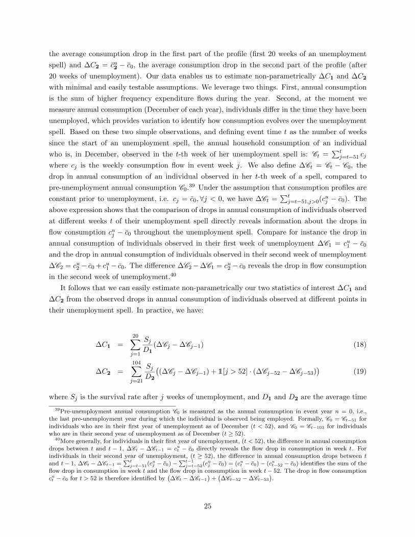
the average consumption drop in the first part of the profile (first 20 weeks of an unemployment
spell) and ∆C2 = cu2 − c0, the average consumption drop in the second part of the profile (after
20 weeks of unemployment). Our data enables us to estimate non-parametrically ∆C1 and ∆C2
with minimal and easily testable assumptions. We leverage two things. First, annual consumption
is the sum of higher frequency expenditure flows during the year. Second, at the moment we
measure annual consumption (December of each year), individuals differ in the time they have been
unemployed, which provides variation to identify how consumption evolves over the unemployment
spell. Based on these two simple observations, and defining event time t as the number of weeks
since the start of an unemployment spell, the annual household consumption of an individual
who is, in December, observed in the t-th week of her unemployment spell is: Ct =∑t
j=t−51 cj
where cj is the weekly consumption flow in event week j. We also define ∆Ct = Ct − C0, the
drop in annual consumption of an individual observed in her t-th week of a spell, compared to
pre-unemployment annual consumption C0.39 Under the assumption that consumption profiles are
constant prior to unemployment, i.e. cj = c0,∀j < 0, we have ∆Ct =∑t
j=t−51,j>0(cuj − c0). The
above expression shows that the comparison of drops in annual consumption of individuals observed
at different weeks t of their unemployment spell directly reveals information about the drops in
flow consumption cuj − c0 throughout the unemployment spell. Compare for instance the drop in
annual consumption of individuals observed in their first week of unemployment ∆C1 = cu1 − c0
and the drop in annual consumption of individuals observed in their second week of unemployment
∆C2 = cu2 − c0 + cu1 − c0. The difference ∆C2−∆C1 = cu2 − c0 reveals the drop in flow consumption
in the second week of unemployment.40
It follows that we can easily estimate non-parametrically our two statistics of interest ∆C1 and
∆C2 from the observed drops in annual consumption of individuals observed at different points in
their unemployment spell. In practice, we have:
∆C1 =
20∑j=1
SjD1
(∆Cj −∆Cj−1) (18)
∆C2 =
104∑j=21
SjD2
((∆Cj −∆Cj−1) + 1[j > 52] · (∆Cj−52 −∆Cj−53)
)(19)
where Sj is the survival rate after j weeks of unemployment, and D1 and D2 are the average time
39Pre-unemployment annual consumption C0 is measured as the annual consumption in event year n = 0, i.e.,the last pre-unemployment year during which the individual is observed being employed. Formally, C0 = Ct−51 forindividuals who are in their first year of unemployment as of December (t < 52), and C0 = Ct−103 for individualswho are in their second year of unemployment as of December (t ≥ 52).
40More generally, for individuals in their first year of unemployment, (t < 52), the difference in annual consumptiondrops between t and t − 1, ∆Ct − ∆Ct−1 = cut − c0 directly reveals the flow drop in consumption in week t. Forindividuals in their second year of unemployment, (t ≥ 52), the difference in annual consumption drops between tand t− 1, ∆Ct −∆Ct−1 =
∑tj=t−51(cuj − c0)−
∑t−1j=t−52(cuj − c0) = (cut − c0)− (cut−52 − c0) identifies the sum of the
flow drop in consumption in week t and the flow drop in consumption in week t− 52. The drop in flow consumptioncut − c0 for t > 52 is therefore identified by
(∆Ct −∆Ct−1
)+(∆Ct−52 −∆Ct−53
).
25

spent in the first and the second part of the benefit schedule.41
To implement this strategy, we start by estimating, on the sample of individuals who are
unemployed in December of any year between 2000 and 2007, the average annual consumption
drops as a function of the time t that individuals have spent unemployed as of December, using the
following specification
∆Ci,t =∑j
βj · 1[t = j] +∑l
ηl · 1[Calendar Yeari,t = l] + εi,t (20)
We display in Figure 6 panel A our baseline estimates of the drop in annual consumption where
in practice, we group individuals in 10 weeks intervals of unemployment duration for estimation.42
Panel A reports βt/C0 = ∆Ct/C0, i.e., we scale our estimates by the average annual consumption in
the last year prior to unemployment, to express consumption drops relative to pre-unemployment
levels. The Figure shows that the drop in annual consumption increases steadily with time spent
unemployed as of December for individuals observed throughout the first year of unemployment,
and then stabilizes around 10% for individuals observed in their second year of unemployment. The
decrease in the first year of unemployment is partly mechanical as individuals who are observed
at a later time t in the spell have spent more time of the year unemployed and thus experienced a
larger drop in annual consumption. Still, the shape of the slope of these estimates reveals all the
necessary information about the evolution of flow consumption throughout the spell.43
Panel A of Figure 6 also reports our non-parametric estimates of the average drops in consump-
tion for both parts of the benefit profile ∆C1 =∑20
j=1SjD1
(βj − βj−1) and ∆C2 =∑104
j=21SjD2
((βj −
βj−1) + 1[j > 52] · (βj−51 − βj−52)). Standard errors are computed using the Delta-method. Our
results suggest that the average drop in (flow) household consumption for individuals in the first
part of the profile is 4.4%, while it is 9.1% on average for individuals in the second part of the
profile. We also report the p-value from a test of equality of ∆C1 and ∆C2 which strongly rejects
that consumption drops are the same in the first and second part of the benefit profile. Our evi-
dence thus indicates that consumption expenditures do significantly decline over the unemployment
spell.44
Robustness Our implementation so far has rested on two assumptions, which we will in-
vestigate next. First, for simplicity we assumed that cj = c0,∀j < 0, or in other words, that
41Note that we censor durations at two years to deal with a few observations without any end date. Hence, oursummation in ∆C2 only goes up to week 104.
42The left hand side variable in specification (20) is a change in levels (and not a log change in consumption). Thereason is that we need the change in levels (and not the log changes) to retrieve higher frequency consumption fromthe annual changes.
43Intuitively, a linear slope in the first year would imply that cuj − c0 = cuk − c0, ∀k, j < 52, which means that flowconsumption drops right at job loss and remains constant after. Concavity in the estimates for the first year wouldindicate that cuj − c0 < cuk − c0,∀k < j < 52, which means that flow consumption continues to decline throughout theunemployment spell.
44Our approach allows to estimate non-parametrically how consumption evolves at, potentially, any frequency overthe unemployment spell. We report for instance in Appendix Figure C-6 the estimated flow consumption drops overthe first year of unemployment at a 10 week frequency.
26

the consumption profile is flat prior to the start of an unemployment spell. To investigate how
consumption profiles evolve prior to the unemployment spell we report in Figure C-1 the annual
log household consumption changes Ci,t − Ci,t−52 as a function of time t since the onset of a spell
(in 5 weeks bins), relative to the last 5 weeks prior to the onset of a spell. We go as far back
as 4 years prior to the onset of a spell, to detect longer anticipation effects. The Figure shows
two interesting patterns. First, the consumption patterns of households are extremely stable in
the 4 years prior to displacement, suggesting no long term anticipation behaviors. Second, there
are no sharp consumption changes immediately preceding displacement, suggesting no significant
short term anticipation behaviors. Overall, this evidence strongly supports the assumption that
flow consumption profiles are flat prior to the onset of an unemployment spell.
The second assumption used in our baseline implementation is that average flow consumption
profiles are similar for individuals observed at different time t in their spell. In practice, the sample
of individuals who survive until t (i.e. individuals with a completed spell length L ≥ t) may differ
from the sample of individuals who survive until t−1 (i.e., individuals with a completed spell length
L ≥ t− 1), and this may bias our estimates if individuals who select into different spell lengths L
differ in their underlying consumption profiles (dynamic selection on consumption profiles). Note,
however, that we can easily relax the assumption that average consumption profiles are independent
of actual spell length. To ensure that we compare the same sample of individuals at different time
t, we estimate separate flow profiles by completed spell length L using the following specification:
∆Ci,t =∑k
∑j
βj,k · 1[t = j] · 1[L = k] +∑l
ηl · 1[Calendar Yeari,t = l] + εi,t
where we break down spell length into 4 brackets: 1 to 20 weeks, 21 to 40 weeks, 41 to 60 weeks,
and longer than 61 weeks. In Panel B of Figure 6 we report our estimates of βt,L, representing
the drops in annual consumption as a function of time spent unemployed for the 4 categories of
completed spell lengths. Results show that the profile of drops in annual consumption is very
similar across spell length, pointing to a limited role for dynamic selection on consumption profiles.
We also report the implied estimates of ∆C1 and ∆C2, allowing for heterogeneity in profiles across
spell length, ∆C1 =∑
k
∑20j=1
Sj,kD1
(βj,k − βj−1,k) and ∆C2 =∑
k
∑104j=21
Sj,kD2
((βj,k − βj−1,k) +1[j >
52] · (βj−52,k − βj−53,k)). Results are very similar to our baseline estimates, and confirm that
flow consumption significantly decreases over the unemployment spell. The average drop in (flow)
household consumption for individuals in the first part of the profile is 4.8%, while it is 9.6% on
average for individuals in the second part of the profile.
Additional Survey Evidence We further investigate the robustness of our results using the
household consumption surveys (HUT) in Appendix C.4. While the HUT sample is much smaller,
and does not have a panel structure, it directly measures flow consumption at the time of the
survey interview. Results from our preferred specification of Table C-3 column (4) suggest that the
drop in the first part of the profile ∆C1 is 4.6% and the drop in the second part of the profile ∆C2
27

is 10.8%. Reassuringly, despite much larger standard errors, these point estimates are remarkably
similar to our baseline estimates using the registry-based measure of consumption.
4.2 Implications for Consumption Smoothing Gains
The empirical evidence presented above indicates that consumption declines significantly over the
unemployment spell. This decline in consumption suggests that the marginal value of unemploy-
ment benefits increases over the spell, evaluated for the flat policy in place in Sweden.
An important outstanding issue is that our empirical analysis considers changes in expenditures.
The question is to what extent expenditures translate into consumption and thus capture the
potential welfare value of unemployment benefits.45 In particular, unemployed workers may try to
re-allocate certain categories of expenditures to smooth the shocks in their consumption. A first
example is the substitution towards home production, which has been analyzed extensively in the
context of retirement (e.g., Aguiar and Hurst [2005]). A second example is the substitution away
from expenditures on durable goods that provide a consumption flow for future periods as well.
The HUT offers insights into the type of consumption goods that households adjust over the
spell. In Table C-4, we investigate how various categories of expenditures evolve over the un-
employment spell. Consumption of non-durable, uncommitted goods, such as food, recreation,
transportation, or restaurants (columns (2),(6),(7) and (8)), drops significantly early on in the
spell and further decreases over the spell.46 More committed expenditures like housing rents paid
by renters (column (4)) do not seem to decline significantly, neither early, nor later in the un-
employment spell.47 Interestingly, we find a larger drop in restaurant expenditures than in food
expenditures, consistent with substitution towards home production. Substitution towards home
production may affect the level of the consumption smoothing gains of UI benefits.48 However,
its effect on the evolution of the consumption smoothing gains of UI over the spell is ambiguous,
and will depend on the relative availability of substitution towards home production for households
that select into long versus short spells.49
Table C-4 also indicates that expenditures on durable goods such as the purchase of new vehicles
45See Campos and Reggio [2016].46Gruber [1997] considers only food consumption using U.S. data from the PSID for the period 1968-1987 and finds
an average drop of 6.8% in the first year of unemployment, which is very similar to our estimates.47Fixed commitments reduce the ability to smooth consumption and can increase the relevant value of γ to translate
consumption drops into welfare (Chetty and Szeidl [2007]).48The sign of the impact of such substitution patterns on the consumption smoothing gains of UI benefits is nev-
ertheless ambiguous. The availability of consumption insurance through home production means that the drop inconsumption will be smaller than the actual drop in expenditures, which decreases the marginal utility of unemploy-ment benefits. At the same time, complementarity between expenditures and household production increases themarginal utility of benefits. The relative magnitude of these two effects will determine the sign of the impact on theconsumption smoothing gains of UI.
49Note that results displayed in Appendix Tables C-5 and C-6 indicate that the expenditure profiles over food,recreation, transportation, or restaurants are not significantly different for households that select into long versusshort spells. This suggests that there is no significant dynamic selection over the spell based on the availability ofsubstitution towards home production.
28

or the purchase of furniture and home appliances (columns (4) and (5)) decline strongly early during
the spell, but increase later during the spell, yet remaining largely below their pre-unemployment
level. These results suggest that the unemployed can initially smooth the marginal utility of
consumption services by shifting spending away from durables, but they lose the capacity to do so
after some time.50 This in turn will tend to further increase the inclining profile of the consumption
smoothing value of UI benefits over the unemployment spell.
To sum up, empirical evidence seems to substantiate that, in the Swedish context, and for
a flat benefit profile, consumption declines over the spell, and that the consumption smoothing
gains of UI benefits are larger after 20 weeks of unemployment than during the first 20 weeks
of unemployment. This conclusion seems robust to the presence of dynamic substitution across
categories of expenditures.
5 Welfare Analysis
This concluding section brings our theoretical and empirical analysis together to provide an evidence-
based assessment of the UI benefit profile in Sweden. We use our empirical estimates to implement
our sufficient-statistics formulae and to shed light on forces underlying how the sufficient statistics
evolve over the unemployment spell. While our formulae allow for a transparent evaluation of local
changes in the policy profile, we also illustrate how a calibrated structural model allows us to go
beyond the local recommendations.
5.1 Sufficient-Statistics Implementation
The welfare consequences of a marginal increase in UI benefits are reported in Table 3. The
first row examines the consequences of a marginal increase in the benefit level b throughout the
unemployment spell; the second row examines the consequences of a marginal increase in the benefit
b1 during the first 20 weeks of unemployment and the third row examines the consequences of a
marginal increase in the benefit b2 after 20 weeks of unemployment. Different columns show the
different components of the welfare impact.
The first column repeats our estimates of the moral hazard costs (Panel IV of Table 2). As noted
before, the estimated moral hazard cost is high overall (all estimates exceed 1), but the cost is 26
percent higher for benefits paid during the first 20 weeks of unemployment compared to those paid
after 20 weeks of unemployment. The second column repeats our estimates of the drops in average
consumption during the first 20 weeks of unemployment and after 20 weeks of unemployment, but
also averaged over the full unemployment spell. We convert the respective consumption drops into
estimates of the consumption smoothing gains CSk, following the implementation in (14), which
relies on a Taylor approximation and homogeneous preferences. As the appropriate value of risk
50Note again that, although results are relatively imprecise due to the small sample size, Appendix Table C-5 indi-cates that dynamic selection based on durable expenditure profiles is not significant. The availability of consumptionsmoothing through shifting expenditures away from durables is not significantly different for households that selectinto long versus short spells.
29
aversion in this context is uncertain, the consumption smoothing gains are reported for a range
of plausible values (see Chetty [2009], Chetty and Finkelstein [2013]) and range between .05 and
.5. Regardless of the level of risk aversion, when risk preferences are homogenous, the estimated
consumption smoothing gains are twice as high for benefits paid later in the spell.
Putting the estimates of the CS gains and the MH costs together indicates that the MH costs
are substantially larger than the CS gains, even for high risk aversion.51 This is true both for
benefits paid to short-term and long-term unemployed and thus suggests that UI benefits are too
generous overall. Indeed, expressing the welfare effects in terms of “benefit-cost” ratio’s CSk/MHk,
we find that the return to the marginal krona spent on the unemployed is substantially lower than
1. These estimates are, however, sensitive to our implementation assumptions including the risk
preference parameter γ, the tax distortion τ and our normalization relative to the value of krona
spent pre-unemployment.52
Comparing the benefit-costs ratio’s for different parts of the policy allows us to formulate
recommendations on the tilt of the benefits profile b1/b2.53 We find that the relative moral hazard
cost MH1/MH2 (= 1.26) is more than twice as high as the relative consumption smoothing gain
CS1/CS2 (= .50). The implied return to the marginal krona spent on the short-term unemployed
is thus at least twice as low compared to the long-term unemployed, indicating that welfare could be
increased by introducing an inclining tilt (b1 < b2) in the flat Swedish benefit profile. Importantly,
this evaluation of the tilt is less sensitive to the above assumptions. In particular, CS1/CS2
does not depend on the preference parameter γ, while MH1/MH2 does not depend on the tax
distortion τ . More generally, our recommendations on the tilt of the benefit profile are robust to
implementation errors that are uncorrelated with the unemployment duration.
In sum, our implementation suggests that on average UI benefits should be decreased and
especially so for the short-term unemployed. The 2001 reform in Sweden did the exact opposite by
increasing the benefit cap for the first 20 weeks of unemployment.
5.2 From Sufficient Statistics to Mechanisms
While the previous local welfare implementation does not need to identify the forces that shape the
sufficient statistics, it is in practice interesting to explore and analyze these forces, for at least two
reasons. First, from a descriptive point of view, it is interesting to understand what mechanisms
can explain the observed patterns of these statistics. Second, from a welfare perspective, in order
51We note again that, although our duration elasticities and consumption drops are estimated from differentsamples, individuals in the two samples are almost identical in terms of observable characteristics and unemploymentdurations as discussed in Section 2.2.
52Note that consumption drops are experienced at the household level. Our analysis only accounts for the con-sumption smoothing gains for the unemployed individual, hereby underestimating the overall consumption smoothinggain of UI.
53Expressing the welfare effects in terms of “cost/benefit”ratio’s (see Hendren [2013]) is a common approach toformulate policy recommendations. Whenever CS1/MH1 > CS2/MH2, welfare can be increased by increasing thetilt b1/b2. Moreover, a budget-balanced increase in the tilt b1/b2 increases welfare if and only if 1+CS1
1+MH1> 1+CS2
1+MH2,
where the ratio’s correspond the so-called “marginal value of public funds”. We show this in Corollary 1 in AppendixSection A.2.
30

to extend our recommendations to non-local variations, one needs to impose more structure on the
data. Investigating what mechanisms drive the estimated sufficient statistics is a useful way to
inform the choice of structural assumptions to impose on the underlying model used to simulate
the welfare consequences of non-local variations, as we do in subsection 5.3.
In order to shed light on mechanisms, we can leverage the fact that different assumptions re-
garding the underlying structure of the model map into different dynamic behaviors of our sufficient
statistics.
5.2.1 Dynamic Profile of Sufficient Statistics
Our sufficient-statistics characterization indicates that, everything else equal, unemployment ben-
efits should decline over the spell when the consumption smoothing gains are lower for benefits
paid later in the spell or when their moral hazard cost is higher. The optimal benefit profile has
been the topic of a series of seminal papers, mostly studying single-agent, stationary environments
(see Shavell and Weiss [1979], Hopenhayn and Nicolini [1997] and Shimer and Werning [2008]).
The relevant forces in a stationary setting and how they affect the optimal benefit profile are well
understood from this literature. We can re-express the impact of these forces on the unemployment
policy through their impact on the gradient of the moral hazard costs and consumption smoothing
gains:54
Proposition 2. Consider a flat benefit profile (bt = b < w − τ for ∀t) in a single-type, stationary
environment (hi,t (·) = h (·) for ∀i, t) with β (1 + r) = 1, T =∞ and assuming differentiability:
(i) when agents are borrowing-constrained throughout the unemployment spell (ai,t = 0 for ∀i, t),
MHt ≤MHt′ and CSt = CSt′ for t < t′.
(ii) when agents are not borrowing-constrained, but preferences are separable (∂vui (c, s) /∂c =
∂vei (c) /∂c = v′ (c)),
CSt < CSt′ for t < t′.
The force underlying the increasing moral hazard cost is the forward-looking behavior of job
seekers. Increasing unemployment benefits later in the spell discourages forward-looking job seekers
already early in the spell and is therefore always more costly than increasing benefits earlier in the
spell. This causes the optimal benefit profile to be declining, as shown before in Shavell and
Weiss [1979] and Hopenhayn and Nicolini [1997]. The force underlying the increasing consumption
smoothing gain is that, when available, unemployed job seekers use liquid assets to smooth their
marginal utility of consumption. As assets are depleted while unemployed, the marginal utility of
consumption and thus the value of unemployment benefits is always higher later in the spell. This
54Appendix Section A.3 provides the proof (closely following ? and Shimer and Werning [2008]) and gauges therobustness of Proposition 2 within a stationary environment.
31

causes the optimal benefit profile to be inclining, as shown before in Shavell and Weiss [1979] and
Shimer and Werning [2008].55
In practice, however, unemployment dynamics are non-stationary. Non-stationary forces, and
dynamic selection in particular, can mitigate the forces underlying Proposition 2 and, when strong
enough, actually reverse the gradient of the sufficient statistics. We discuss this below in relation to
our empirical estimates, but also develop this argument formally in Appendix Section A.4.56 While
characterizing the impact of non-stationarities on the optimal policy is challenging and previous
work has mostly relied on calibrated models (e.g., Shimer and Werning [2006] and Pavoni [2009]),
our framework provides an alternative approach, which is to analyze how non-stationary forces
affect the gradient of the moral hazard costs and consumption smoothing gains respectively.
In the end, how both the consumption smoothing gains and moral hazard costs evolve over the
unemployment spell remains an empirical question. Yet, because different assumptions regarding
the underlying structure of dynamic models of unemployment map into different dynamic behaviors
of our sufficient statistics, we can use our estimated sufficient statistics to shed interesting light
on the relative importance of different mechanisms in shaping consumption smoothing and moral
hazard over the spell.
5.2.2 Moral Hazard Cost
Our empirical analysis indicates that the moral hazard costs increase over the unemployment spell
in Sweden, suggesting the importance of non-stationary forces dominating the forward-looking
incentives. To illustrate how these forces shape the dynamics of moral hazard costs over the spell,
we can use the earlier expression (11) to re-write the moral hazard cost of an increase in benefit
level b2 after 20 weeks of unemployment, as the sum of two parts,
MH2 =b+ τ
b× εDB ,b2 +
b+ τ
b× [
D1
D2εD1,b2 + εSB ,b2 ].
The first part captures the response in the remaining duration of unemployment, conditional on
still being unemployed at time B = 20 weeks (DB ≡ ΣT−Bs=0 SB+s/SB). In a stationary, single-
agent environment, this first part is the same for any time B and equal to the moral hazard cost
of an overall increase in the benefit level MHb. The second part captures the forward-looking
incentives by which an increase in benefits in the second part of the policy reduces the exit out of
unemployment in the first part of the spell (D1) and increases the survival rate into the second
55Due to the opposing forces coming from moral hazard and consumption smoothing, even in a stationary envi-ronment, deriving the optimal timing of benefits is difficult. Werning [2002] and Shimer and Werning [2008] analyzethese two opposing forces in models with both search and savings being endogenous and show that they exactlycancel out in case of CARA preferences; a flat benefit profile is optimal conditional on the unemployed having accessto liquidity.
56Appendix Section A.4 starts from a specific stationary, search environment with borrowing-constrained agents(subsection A.4.2). We then consider depreciation in the returns to search over the unemployment spell (subsectionA.4.3) and unobservable heterogeneity in the returns to search (subsection A.4.4). We finally allow for unobservablesavings and consider heterogeneity in assets or preferences. We show how the extensions can mitigate and/or reversethe difference in moral hazard costs or consumption smoothing gains at different times during unemployment spell.
32

part of the spell (SB). This second part converges to zero as B goes to 1. Following the argument
in Shavell and Weiss [1979], the forward-looking incentives drive the result that in a stationary
environment the moral hazard cost of increasing unemployment benefits is higher when timed
later in the spell (see Proposition 2). We find the exact opposite in the Swedish context, which
necessitates the presence of significant non-stationary forces that reduce the responsiveness of job
seekers to changes in the policy later in the spell.
Evidence of Forward-looking Behavior We first note that our results unambiguously
show that unemployed individuals are indeed forward-looking. We already reported the estimated
elasticity of D1, the time spent on the first part of the profile, with respect to benefits b2 received in
the second part of the profile is positive and significant (εD1,b2 = .60 (.11), see Table 2). We can also
study the effect of UI benefits on the hazard rates out of unemployment. Figure B-1 in Appendix
Section B.1 reports the corresponding RKD estimates and clearly shows that benefits b2 received
after 20 weeks do have a negative effect on the hazard rate in the first 20 weeks. Unemployed
individuals are thus not fully myopic: they react early in the spell to variation in benefits paid later
in the spell.
Evidence on Non-stationary Forces To highlight the non-stationary forces underlying the
reversed pattern of moral hazard costs in the Swedish context, we compare at different spell lengths
t, the elasticity of the remaining duration Dt ≡ ΣT−ts=0St+s/St with respect to the overall benefit
level b. In a stationary, single-agent environment, these elasticities would remain constant and
be equal to εD,b.57 Instead, our estimates, reported in Figure 4, show that the elasticity of the
remaining duration strongly declines as a function of t. Five months into the spell the elasticity is
only one third of the elasticity at the onset of the spell. This evidence of strong non-stationarities
is corroborated in Appendix Figure B-1 which shows that the effect of UI benefits b on hazard
rates is mostly concentrated in the first two to three months. After three months, the effect of UI
benefits on the hazard rate is small and almost always insignificant.
Both depreciation and heterogeneity in the returns to search can explain why the responsiveness
of exit rates decreases substantially over the unemployment spell. The reduced responsiveness to
changes in the benefit profile, either through depreciation or through selection, makes it less costly
to increase benefits later in the spell. While depreciation by itself cannot, selection - when strong
enough - can in fact reverse the decline of moral hazard costs over the spell, as shown in Appendix
Section A.4. Separating true depreciation from selection on heterogeneity in returns to search is
notoriously difficult and beyond the scope of this paper, but our analysis nevertheless suggests the
importance of embedding such non-stationary features in dynamic models of unemployment.
57Because exit rates only depend on the continuation policy in a stationary environment and there are no selectioneffects in a single-agent environment in response to policy variation earlier in the spell, the elasticity of the remainingduration Dt with respect to an overall change in the benefit level is independent of t.
33

5.2.3 Consumption Responses
We now turn to the dynamic profile of the consumption smoothing gains. We find that the average
consumption drop is more pronounced later in the spell. We therefore revisit mechanisms that can
explain this pattern and whether they necessarily translate in consumption smoothing gains that
increase over the spell.
Assets and Liquidity Constraints As stated above, a single-agent model of intertemporal
consumption predicts that the marginal utility of consumption is weakly increasing during the
unemployment spell. Intuitively, long-term unemployment implies a larger shock in resources, so we
expect the unemployed to run down their assets and consume less the longer they are unemployed.
Or they become liquidity-constrained and start consuming “hand-to-mouth”.
We find clear evidence of the role of assets and liquidity constraints in determining the con-
sumption smoothing over the spell. First, following the same methodology as in Figure 6, we
report the average annual consumption drops by time spent unemployed as of December, but now
breaking down the sample by the level of net wealth of the household at the start of the spell.
As shown in Appendix Figure C-2, individuals with higher net wealth experience a lower drop
in consumption. Second, we provide direct evidence that individuals do use their liquid assets to
smooth consumption over the spell. Appendix Figure C-3 displays the relative change in liquid
bank asset holdings by time spent unemployed. The Figure shows that individuals use their liquid
assets to smooth consumption, especially earlier on in the spell, by depleting their bank accounts
or reducing their savings. Finally, evidence from registry data also indicates that debt does not
offer much help in smoothing consumption over the unemployment spell, hinting at the presence
of liquidity constraints. In Appendix Figure C-4, we provide evidence of a reduction in the use of
non mortgage-related credit over the unemployment spell. This suggests that as the duration of
the spell increases, access to credit becomes harder and consumption out of debt falls significantly.
Overall, this analysis confirms that assets and debt may offer means to smooth consumption
over short spells. But as the unemployment spell continues, these means get quickly exhausted.
Households in the second part of the profile seem therefore closer to being hand-to-mouth.
Spousal Labor Supply Within a household, the labor supply of other members of the
household may help reduce the drop in household consumption over the spell. In Figure C-5 we
investigate how the labor supply of other members of the household affects the drop in household
consumption over the spell. Following the same methodology as in Figure 6, we report the average
change in total earnings and in total disposable income of all other members of the household as
a function of time spent unemployed, scaled by the annual household consumption level prior to
unemployment. Results show that within-household changes in the earnings and disposable income
of all other members of the household are small and almost never significantly different from zero
throughout the unemployment spell. This suggests that in our context, labor supply responses of
other household members is not playing a significant role in increasing household consumption in
34

response to an unemployment shock, even for long-term unemployed.
Dynamic Selection In practice, agents are heterogeneous and selection into longer unem-
ployment spells may affect consumption responses over the spell and the gradient of consumption
smoothing gains. As shown in Appendix Section A.4.5), if those selecting into longer unemploy-
ment spells suffer less from a drop in consumption, the positive gradient of consumption smoothing
benefits due to the falling consumption is reduced and can potentially be reversed.
In theory, as long as preferences are homogeneous, we can use the approximation in condition
(14) to translate the average consumption wedge into the consumption smoothing gains of increasing
benefits. When preferences are heterogeneous, the consumption smoothing gains are approximated
(using Taylor expansions of v′(cui,t
)around ci,0 for each individual) by
CSt ∼=Eut [v′i (ci,0)]− E0 [v′i (ci,0)]
E0 [v′i (ci,0)]−Et
[v′′i (ci,0)
(ci,0 − cui,t
)]E0 [v′i (ci,0)]
, (21)
where Eut takes the weighted average among the unemployed at time t (with weights Si,t/St) and
E0 takes the average before the onset of the unemployment spell. The first part of this expression
indicates that the consumption smoothing gains of long-term benefits will be reduced if individuals
with lower marginal utility of consumption remain unemployed for longer. The second part of this
expression indicates that the consumption smoothing gains are reduced if households with lower
risk aversion and or lower consumer drops remain unemployed for longer.58
Our analysis of the consumption profiles by completed spell length already suggested that the
dynamic selection on consumption profiles was limited (see Figure 6, Section 4.1). To further
assess the potential magnitude of dynamic selection, we investigate in Appendix Table C-1 how
various observable characteristics that have been shown to correlate with consumption and risk
preferences are distributed across short term and long term unemployed. The patterns of selection
are generally small in magnitude and often ambiguous in sign. Income levels and net wealth
levels have quantitatively small and non-monotonic effects on the probability to select into longer
spells. Compared to households with no or negative net wealth, households with some small
wealth (<500kSEK≈ 55kUSD) have a slightly lower probability to be long term unemployed. But
individuals with high net wealth have a slightly higher probability to select into long spells. This
result suggests that in our context, individuals with better means to smooth consumption do
not unambiguously select into longer spells, which corroborates the evidence of no clear patterns
of selection on consumption profiles. Also portfolio characteristics (i.e., the fraction of portfolio
wealth invested in stocks, and leverage defined as total debt divided by gross assets), which have
been shown to be correlated with risk preferences, have small and non-monotonic impacts on the
probability to experience a long unemployment spell. In contrast, the probability of experiencing
58Note that if preferences are heterogeneous within the group of unemployed at a given time during the unemploy-ment spell, any negative correlation between the drop in consumption and risk aversion, would further reduce theconsumption smoothing gains (see Andrews and Miller [2013]).
35

long unemployment spells (1[L > 20 wks]) is significantly and monotonically correlated with age.
However, existing evidence from the literature suggests a U-shape relationship between age and
risk aversion (Cohen and Einav [2007]), so the dynamic selection on age has an ambiguous effect
on the evolution of risk preferences over the spell.
Overall, the observed dynamic selection patterns on consumption and risk preferences do not
suggest that relative consumption smoothing gains would be significantly different than our esti-
mates based on the average drops in consumption.
5.3 Beyond Local Recommendations
Our local recommendation regarding the policy and the tilt in particular may not be informative
about how the optimal policy should look like.59 To go beyond our local recommendations, we
need to know how the sufficient statistics vary with the policy parameters. We briefly illustrate
how this can be explored using the structure of a model. That is, we calibrate a rich, non-stationary
structural model to match the sufficient statistics for local policy evaluation and simulate how these
sufficient statistics change when moving away from the local policy.
We describe the details of the calibration and simulation in Appendix D. We consider a model
with CRRA preferences and additive search costs like in Hopenhayn and Nicolini [1997], Lentz
and Traneas [2005] and Chetty [2008a], but motivated by the evidence discussed in the previous
subsection we allow for an exit rate function with heterogeneous returns to search that depreciate
exponentially and for a heterogeneous asset distribution at the start of the unemployment spell.
As our calibration targets our sufficient statistics estimates, the structural model delivers the same
local recommendations around the existing policy. That is, the flat benefit b = .72 is too generous
overall and especially so for the short-term unemployed.
Figure 7 illustrates how the moral hazard costs and consumption smoothing gains change when
reducing the overall generosity of the policy in our calibrated model. Two findings emerge. First,
the consumption smoothing gains increase while the moral hazard costs decrease as we reduce
the benefit level.60 In particular, CSb and MHb are equalized for a flat replacement of b = .58.
Second, as we decrease the overall generosity, the consumption smoothing gains remain higher for
benefits paid to the long-term unemployed (CS2 > CS1), while the moral hazard costs remain lower
(MH2 < MH1). The introduction of an inclining tilt (b2 > b1) thus remains welfare-improving
for lower replacement rates. In particular, our model predicts that welfare would be maximized by
setting b1 = .48 for the short-term unemployed and b2 = .68 for the long-term unemployed (while
keeping the tax rate unchanged).
In Appendix D we further illustrate the complementary value of the structural approach and
sufficient-statistics approach. In particular, we explore how our findings depend on the assump-
59Of course, this issue may also arise for a one-dimensional change in benefit level bk. Only if the policy problem isstrictly concave in all benefit levels, can we be certain that a welfare-increasing change in the benefit level bk actuallymoves the policy closer to the optimal policy.
60Note that we keep the asset distribution at the start of unemployment fixed, while this is likely to respond to thegenerosity of the unemployment policy.
36

tions of the non-stationary features of the search environment and the assumptions made for our
consumption-based implementation of the consumption smoothing gains.61
6 Conclusion
This paper has offered a simple, general and empirically implementable framework to evaluate the
optimal time profile of unemployment benefits. Our theoretical approach proves that, independent
of the underlying primitives of the model, the dynamic problem of balancing insurance value and
incentive costs can be characterized in a transparent way as a series of simple trade-offs involving
just a few estimable statistics. Putting this simple characterization to the data, our empirical
implementation has shown that it is not at all obvious that declining benefit profiles are always
optimal. Despite the forward-looking behavior of job seekers, important non-stationary forces can
make the moral hazard costs of benefits offered to the long-term unemployed higher than the costs
of benefits offered early in the spell. The limited access to consumption smoothing opportunities
that we document among the unemployed in Sweden also makes cutting benefits particularly costly
for the long-term unemployed.
We have presented a framework that is easily replicable and our hope is that it will trigger
new empirical work that analyzes the relevant statistics for policy evaluation in other contexts
where labor market conditions, access to credit or the unemployment policy may be very different.
Our analysis has shown that the empirical analysis of labor supply responses to UI should pay
particular attention to the timing of benefits in order to produce estimates that can be meaningful
from a welfare perspective. In terms of assessing the value of UI benefits, our analysis shows that
fruitful avenues of research are being opened by administrative and/or proprietary data on wealth
and expenditures matched with UI records. Most importantly, the tools developed in this paper
can be applied to other dynamic contexts. An important area for future work will be to develop
such simple, yet robust characterization of various other dynamic policies, including the design of
retirement pensions or parental leave policies.
61In line with Chetty [2006], we find that for CRRA preferences the Taylor approximation of the marginal utilitiessubstantially underestimates the consumption smoothing gains (by more than 20% for γ = 2). The approximationerror on the relative consumption smoothing gains, however, is much smaller (equal to 5% for γ = 2), leaving therecommendation on the tilt basically unaffected.
37

References
Acemoglu, Daron, “Public Policy in a Model of Long-term Unemployment,” Economica, 1995, 62 (246), 161–178.
Aguiar, Mark and Erik Hurst, “Consumption versus Expenditure,” Journal of Political Economy, 2005, 113 (5), pp.
919–948.
Alvarez, Fernando E., Katarına Borovickova, and Robert Shimer, “Decomposing Duration Dependence in a Stopping
Time Model,” Working Paper 22188, National Bureau of Economic Research April 2016.
Andrews, Isaiah and Conrad Miller, “Optimal Social Insurance with Heterogeneity,” Mimeo, MIT, 2013.
Baily, Martin N., “Some Aspects of Optimal Unemployment Insurance,” Journal of Public Economics, 1978, 10 (3),
379–402.
Blanchard, Olivier Jean and Peter Diamond, “Ranking, Unemployment Duration, and Wages,” The Review of Eco-
nomic Studies, 1994, 61 (3), 417–434.
Browning, Martin and Søren Leth-Petersen, “Imputing consumption from income and wealth information,” The
Economic Journal, 2003, 113 (488), F282–F301.
Campos, Rodolfo G and Iliana Reggio, “Optimal unemployment insurance: Consumption versus expenditure,” Labour
Economics, 2016, 38, 81–89.
Card, David, David S. Lee, Zhuan Pei, and Andrea Weber, “Inference on Causal Effects in a Generalized Regression
Kink Design,” Econometrica, 2015, 83 (6), 2453–2483.
Chetty, Raj, “A General Formula for the Optimal Level of Social Insurance,” Journal of Public Economics, 2006, 90
(10-11), 1879–1901.
, “Moral Hazard versus Liquidity and Optimal Unemployment Insurance,” Journal of Political Economy, 2008,
116 (2), 173–234.
, “Sufficient Statistics for Welfare Analysis: A Bridge Between Structural and Reduced-Form Methods,” Annual
Review of Economics, 05 2009, 1 (1), 451–488.
and Adam Szeidl, “Consumption Commitments and Risk Preferences,” The Quarterly Journal of Economics,
2007, 122 (2), pp. 831–877.
and Amy Finkelstein, “Chapter 3 - Social Insurance: Connecting Theory to Data,” in Martin Feldstein Alan
J. Auerbach, Raj Chetty and Emmanuel Saez, eds., handbook of public economics, vol. 5, Vol. 5 of Handbook of
Public Economics, Elsevier, 2013, pp. 111 – 193.
Cohen, Alma and Liran Einav, “Estimating Risk Preferences from Deductible Choice,” American Economic Review,
2007, 97 (3), 745–788.
Coles, Melvyn G. and Eric Smith, “Marketplaces and Matching,” International Economic Review, 1998, 39 (1),
239–254.
Couch, Kenneth A and Dana W Placzek, “Earnings losses of displaced workers revisited,” The American Economic
Review, 2010, 100 (1), 572–589.
den Berg, Gerard Van, “Nonstationarity in Job Search Theory,” The Review of Economic Studies, 1990, 57 (2),
255–277.
Eckstein, Zvi and Gerard Van den Berg, “Empirical labor search: A survey,” Journal of Econometrics, 2007, 136 (2),
531 – 564. The interface between econometrics and economic theory.
Eika, L., M. Mogstad, and O. Vestad, “”What Can We Learn About Household Consumption From Information on
Income and Wealth”,” working paper, 2017.
Ganong, Peter and Simon Jaeger, “A Permutation Test and Estimation Alternatives for the Regression Kink Design,”
Harvard University Discussion Paper, 2014.
Gruber, Jonathan, “The Consumption Smoothing Benefits of Unemployment Insurance,” American Economic Review,
38

1997, 87 (1), 192–205.
Hendren, Nathaniel, “The Policy Elasticity,” Working Paper 19177, National Bureau of Economic Research June
2013.
Hopenhayn, Hugo A. and Juan Pablo Nicolini, “Optimal Unemployment Insurance,” Journal of Political Economy,
1997, 105 (2), 412–438.
Koijen, Ralph, Stijn Van Nieuwerburgh, and Roine Vestman, Judging the Quality of Survey Data by Comparison with
Truth as Measured by Administrative Records: Evidence From Sweden, University of Chicago Press, July 2014.
Kreiner, Claus T., David Dreyer Lassen, and Søren Leth-Petersen, “Liquidity Constraint Tightness and Consumer
Responses to Fiscal Stimulus Policy,” Mimeo, Copenhagen University, 2014.
Kroft, Kory, Fabian Lange, and Matthew J. Notowidigdo, “Duration Dependence and Labor Market Conditions:
Evidence from a Field Experiment,” The Quarterly Journal of Economics, 2013.
Krueger, Alan B. and Bruce D. Meyer, “Labor Supply Effects of Social Insurance,” Handbook of Public Economics,
Elsevier 2002.
Landais, Camille, “Assessing the Welfare Effects of Unemployment Benefits Using the Regression Kink Design,”
American Economic Journal: Economic Policy, 2015.
, Pascal Michaillat, and Emmanuel Saez, “Optimal Unemployment Insurance over the Business Cycle,” Working
Paper 16526, National Bureau of Economic Research 2010.
Lehr, Brandon, “Optimal Unemployment Insurance with Endogenous Negative Duration Dependence,” Public Fi-
nance Review, 2017, 45 (3), 395–422.
Lentz, Rasmus and Torben Traneas, “Job Search and Savings: Wealth Effects and Duration Dependence,” Journal
of Labor Economics, July 2005, 23 (3), 467–490.
Ljungqvist, Lars and Thomas J. Sargent, “The European Unemployment Dilemma,” Journal of Political Economy,
1998, 106 (3), 514–550.
Lockwood, Ben, “Information Externalities in the Labour Market and the Duration of Unemployment,” The Review
of Economic Studies, 1991, 58 (4), 733–753.
Machin, Stephen and Alan Manning, “The Causes and Consequences of Longterm Unemployment in Europe,” in
Orley C. Ashenfelter and David Card, eds., Handbook of Labor Economics, Vol. 3, Part C of Handbook of Labor
Economics, Elsevier, 1999, pp. 3085 – 3139.
Mas, Alexandre and Andrew Jonhston, “Potential Unemployment Insurance Duration and Labor Supply: the Indi-
vidual and Market-Level Response to a Benefit Cut,” Mimeo, Princeton University, 2015.
McCrary, Justin, “Manipulation of the Running Variable in the Regression Discontinuity Design: A Density Test,”
Journal of Econometrics, February 2008, 142 (2), 698–714.
Meyer, Bruce, “Unemployment Insurance and Unemployment Spells,” Econometrica, 1990, 58(4), 757–782.
, “Do Matching Frictions Explain Unemployment? Not in Bad Times,” American Economic Review, June 2012,
102 (4), 1721–50.
Mogstad, Magne and Andreas Kostol, “Earnings, Income, and Consumption of Alowed and Rejected Disability
Insurance Applicants,” American Economic Review, Papers and Proceedings, 2015, 105 (5), 137–141.
Nekoei, Arash and Andrea Weber, “Does Extending Unemployment Benefits Improve Job Quality?,” IZA Discussion
Papers 9034, Institute for the Study of Labor (IZA) April 2015.
Pavoni, Nicola, “Optimal Unemployment Insurance, With Human Capital Depreciation, and Duration Dependence,”
International Economic Review, 2009, 50 (2), 323–362.
Pistaferri, Luigi, “Household Consumption: Research Questions, Measurement Issues, and Data Collection Strate-
gies,” Mimeo Stanford University, 2015.
39

Rothstein, Jesse, “Unemployment Insurance and Job Search in the Great Recession,” Working Paper 17534, National
Bureau of Economic Research October 2011.
Schmieder, Johannes F and Till Von Wachter, “The Effects of Unemployment Insurance Benefits: New Evidence and
Interpretation,” Annual Review of Economics, 2016, 8, 547–581.
, , and , “The Effects of Extended Unemployment Insurance Over the Business Cycle: Evidence from Re-
gression Discontinuity Estimates Over 20 Years,” The Quarterly Journal of Economics, 2012, 127 (2), 701–752.
Shavell, Steven and Laurence Weiss, “The Optimal Payment of Unemployment Insurance Benefits over Time,” Journal
of Political Economy, 1979, 87 (6), 1347–1362.
and Ivan Werning, “On the Optimal Timing of Benefits with Heterogeneous Workers and Human Capital Depre-
ciation ,” 2006.
and , “Reservation Wages and Unemployment Insurance,” Quarterly Journal of Economics, 2007, 122 (3),
1145–1185.
and , “Liquidity and Insurance for the Unemployed,” American Economic Review, 2008, 98 (5), 1922–42.
Singh, S. and G. Maddala, “A Function for the Size Distribution of Incomes,” Econometrica, 1976, 44 (5), 963–970.
Spinnewijn, Johannes, “Unemployed but Optimistic: Optimal Insurance Design with Biased Beliefs,” Journal of the
European Economic Association, 2015, 13 (1), 130–167.
Valletta, Robert and Henry S. Farber, “Extended Unemployment Insurance and Unemployment Duration in The
Great Recession: The U.S. Experience,” Mimeo, Princeton University, 2011.
Werning, Ivan, “Optimal Unemployment Insurance with Unobservable Savings,” University of Chicago and UTDT,
2002.
40

Appendix
Figure 1: Sufficient statistics for welfare analysis of two-part policy
A. Unemployment response wrt b1
A.I Policy variation A.II Survival Function
B
db1
0U
I ben
efits
0Unemployment duration
Flat profile b1 = b2
Decreasing profile b1 > b2
D1 D2
dD1
eD1, b1 = dD1/db1 * b1/D1
dD2
eD2, b1 = dD2/db1 * b1/D2
B
0S
urvi
val r
ate
0Unemployment duration
B. Unemployment response wrt b2
B.I Policy variation B.II Survival Function
B
db2
0U
I ben
efits
0Unemployment duration
Flat profile b1 = b2
Increasing profile b1 < b2
D1 D2
dD2
eD2, b2 = dD2/db2 * b2/D2
dD1
eD1, b2 = dD1/db2 * b2/D1
B
0S
urvi
val r
ate
0Unemployment duration

Figure 1: Sufficient statistics for welfare analysis of two-part policy (continued)
C. Consumption profile for current policy
C.I Current Policy C.II Consumption Profile
b1 = b2
B
0U
I ben
efits
0Unemployment duration
B
c0
cut
Δc1 Δc2
CSk ≅ γ Δck / c0
Δck = Σ St cut / Dk - c0
0C
onsu
mpt
ion
0Unemployment duration
Notes: The figure summarizes the policy variation and statistics needed to characterize an optimal two-part profilegiving b1 for the first B weeks and b2 afterwards. In Panel A, we display policy variation db1 in benefits given for thefirst B weeks that allows evaluating the moral hazard cost of a change in b1, MH1. The moral hazard cost dependson the responses of the duration spent in the first part of the profile D1 and in the second part of the profile D2, asexemplified in the right panel. These responses enable the identification of the cross-duration elasticities εD1,b1 andεD2,b1 entering the RHS of the corresponding dynamic Baily-Chetty formula (11). Since we start from a flat profile,as is the case in our empirical application in Sweden, the response in total unemployment duration D is in principlesufficient, following equation (6). In Panel B, we display policy variation that allows to evaluate the moral hazardcost of a change in b2. Like in Panel A, we start from a flat profile and display variation db2 in benefits given afterB weeks, which enables the identification of the cross-duration elasticities εD1,b2 , εD2,b2 entering the RHS of thecorresponding dynamic Baily-Chetty formula. To evaluate the consumption smoothing gains of the two-part policy,following the implementation in (14), the planner requires the average drop in consumption ∆c1 for individuals inthe first part of the profile receiving b1, and the average drop in consumption ∆c2 for individuals in the second partof the profile receiving b2. This can be calculated based on the profile of consumption as a function of time spentunemployed as depicted in Panel C. Note that these consumption statistics need to be evaluated at the current profile,and do not require any policy variation.
42

Figure 2: UI benefits and unemployment duration as a function of daily wage aroundthe 725SEK threshold
A. 1999 - 2000
A.I UI schedule A.II Unemployment duration
1999-2000Kink in b1 and b2
475
525
575
625
675
Dai
ly B
enefi
ts (S
EK)
600 650 700 750 800 850Daily Wage (SEK)
b1: benefit for the first 20 wksb2: benefits after 20 wks
Kink in b1 and b2
1520
2530
35D
urat
ion
of u
nem
ploy
men
t spe
ll
600 650 700 750 800 850Daily Wage (SEK)
B. 2001
B.I UI schedule B.II Unemployment duration
2001Kink in b2
475
525
575
625
675
Dai
ly B
enefi
ts (S
EK)
600 650 700 750 800 850Daily Wage (SEK)
b1: benefit for the first 20 wksb2: benefits after 20 wks
Kink in b2 only
1520
2530
35D
urat
ion
of u
nem
ploy
men
t spe
ll
600 650 700 750 800 850Daily Wage (SEK)
43

Figure 2: UI benefits and unemployment duration as a function of daily wage aroundthe 725SEK threshold (continued)
C. 2002-2007
C.I UI schedule C.II Unemployment duration
2002-2006No Kink
475
525
575
625
675
Dai
ly B
enefi
ts (S
EK)
600 650 700 750 800 850Daily Wage (SEK)
b1: benefit for the first 20 wksb2: benefits after 20 wks
No kink
1520
2530
35D
urat
ion
of u
nem
ploy
men
t spe
ll
600 650 700 750 800 850Daily Wage (SEK)
Notes: The left panels display the UI benefit level received during the first 20 weeks of unemployment (b1) and after20 weeks of unemployment (b2) as a function of daily wage prior to becoming unemployed. For spells starting beforeJuly 2001 (A.I), the schedule exhibits a kink in both b1 and b2 at the 725SEK threshold, which can be used to identifythe effect of both b1 and b2 on unemployment duration. For spells starting between July 2001 and July 2002 (B.I),the schedule exhibits a kink in b2 only at the 725SEK threshold, which can be used to identify the effect of b2 onunemployment duration. Finally, for spells starting after July 2002 (C.I), the schedule is linear for both b1 and b2 atthe 725SEK threshold, which offers a placebo setting to assess the validity of the RK design at the 725SEK threshold.The right panels plot average unemployment duration in bins of previous daily wage for the three periods of interest.Unemployment duration is defined as the number of weeks between registration at the PES and exiting the PESor finding any employment (part-time or full-time employment, entering a PES program with subsidized work ortraining, etc.). Unemployment duration is capped at two years. Sample is restricted to unemployed individuals withno earnings who report being searching for full-time employment. The graphs provide graphical evidence of a changein slope in the relationship between unemployment duration and previous daily wage in response to the kink in UIbenefits. The change in slope is larger for spells starting before July 2001, when both b1 and b2 are capped at the725SEK threshold (A.II). The magnitude of the change in slope decreases for spells starting between July 2001 andJuly 2002 when only b2 is capped at the 725SEK threshold. Finally, there is no significant change in slope for spellsafter July 2002, when the schedule is linear for both b1 and b2 at the threshold, which is supportive of the identifyingassumptions of the RK design. Formal estimates of the change in slope using linear specifications of the form ofequation (16) are displayed in Table 2. The red lines display predicted values of the regressions in the linear case.
44
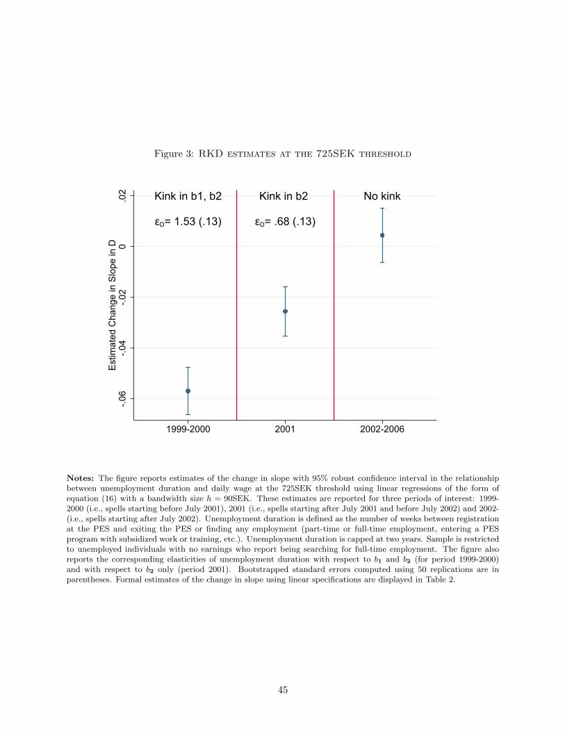
Figure 3: RKD estimates at the 725SEK threshold
Kink in b1, b2 Kink in b2 No kink
εD= 1.53 (.13) εD= .68 (.13)
-.06
-.04
-.02
0.0
2Es
timat
ed C
hang
e in
Slo
pe in
D
1999-2000 2001 2002-2006
Notes: The figure reports estimates of the change in slope with 95% robust confidence interval in the relationshipbetween unemployment duration and daily wage at the 725SEK threshold using linear regressions of the form ofequation (16) with a bandwidth size h = 90SEK. These estimates are reported for three periods of interest: 1999-2000 (i.e., spells starting before July 2001), 2001 (i.e., spells starting after July 2001 and before July 2002) and 2002-(i.e., spells starting after July 2002). Unemployment duration is defined as the number of weeks between registrationat the PES and exiting the PES or finding any employment (part-time or full-time employment, entering a PESprogram with subsidized work or training, etc.). Unemployment duration is capped at two years. Sample is restrictedto unemployed individuals with no earnings who report being searching for full-time employment. The figure alsoreports the corresponding elasticities of unemployment duration with respect to b1 and b2 (for period 1999-2000)and with respect to b2 only (period 2001). Bootstrapped standard errors computed using 50 replications are inparentheses. Formal estimates of the change in slope using linear specifications are displayed in Table 2.
45

Figure 4: Testing for stationarity: elasticity of the remaining duration of unem-ployment, conditional on surviving until t, with respect to changes in the flatbenefit level
0.5
11.
52
Estim
ated
ela
stic
ity o
f rem
aini
ng d
urat
ion
cond
ition
al o
n su
rviv
al
0 1 2 3 4 5Time t since start of spell (months)
Notes: The figure reports RKD estimates (with 95% robust confidence interval) of the elasticity of the remainingduration of unemployment conditional on surviving until t with respect to changes in the flat benefit level b. Estimatesuse the presence, for spells starting before July 2001, of a kink in the benefit schedule of the flat benefit b at the 725SEKwage threshold. We use polynomial regressions of the form of equation (16) with a bandwidth size h = 100SEK.The remaining duration Dt is the unemployment duration D minus t, conditional on being still unemployed aftert months. Unemployment duration is defined as the number of weeks between registration at the PES and exitingthe PES or finding any employment (part-time or full-time employment, entering a PES program with subsidizedwork or training, etc.). Sample is restricted to unemployed individuals with no earnings who report being searchingfor full-time employment. In a stationary environment, the elasticity of Dt with respect to the flat benefit b shouldbe constant with t. As the estimated elasticities strongly decline with t, our results suggest the presence of strongnon-stationary forces (i.e., dynamic selection, duration-dependence, etc.).
46

Figure 5: Estimated Change in Log Annual Consumption as a Function of Time SinceStart of Unemployment Spell
Average log consumption dropin year n = 1:
-.054 (.001)
-.125
-.1-.0
75-.0
5-.0
250
.025
Cha
nge
in L
og A
nnua
l Con
sum
ptio
n R
elat
ive
to P
re-U
nem
ploy
men
t
-4 -3 -2 -1 0 1 2 3 4 5 6Year Relative to Start of Unemployment Spell
Notes: The Figure analyzes changes in log annual household consumption from our registry-based measure ofconsumption expenditures at unemployment, following the standard approach in the literature (e.g. Gruber [1997]).We define event year n = 1 as the year an unemployment spell starts, and focus on individuals who are observedunemployed in December of year n = 1, and who were employed in December of year n = 0. We report coefficientestimates from the event year dummies γj from event study specification (17). Coefficients are relative to event yearn = 0. See text for details.
47

Figure 6: Estimated Drop in Annual Consumption Relative to Pre-Unemployment asa Function of Time Spent Unemployed
A. Baseline Estimates
Estimated Drop in Consumption (Flow)First 20 weeks: ∆c1 = -.0441 (.01)After 20 weeks: ∆c2 = -.091 (.005)Test ∆c1 = ∆c2: p-value = 0
-.2-.1
5-.1
-.05
0.0
5D
rop
in A
nnua
l Con
sum
ptio
n R
elat
ive
to P
re-U
0 10 20 30 40 50 60 70 80 90 100Number of Weeks Unemployed
B. Profile Heterogeneity by Completed Spell Length
Estimated Drop in Log Consumption (Flow)First 20 weeks (weighted average): ∆c1 = -.0477 (.0079)After 20 weeks (weighted average): ∆c2 = -.0958 (.0158)
-.2-.1
5-.1
-.05
0.0
5D
rop
in A
nnua
l Con
sum
ptio
n R
elat
ive
to P
re-U
0 10 20 30 40 50 60 70 80 90 100Number of Weeks Unemployed
1-20 wks. 21-40 wks.41-60 wks. 61-100 wks.
Notes: This Figure shows average annual consumption drops compared to pre-unemployment ∆Ct by time t spentunemployed as of December (when annual consumption is observed in the registry data), and uses this variation tonon-parametrically estimate the evolution of higher frequency household consumption throughout the unemploymentspell. Panel A reports βt/C0 = ∆Ct/C0, i.e. estimates from equation (20) scaled by the average annual consumptionin the last year prior to unemployment, so that all consumption drops are expressed relative to pre-unemploymentlevels. The Figure also reports non-parametric estimates of the average drops in consumption in each parts of the
benefit profile ∆C1 and ∆C2 following the methodology explained in subsection 4.1. Standard errors are computed
using the Delta-method. We also report the p-value from a test of equality of ∆C1 and ∆C2. In Panel B, we estimateseparate profiles ∆Ct,k=1,.,4 for 4 categories of total completed spell length L, and report estimates of ∆C1 and ∆C2
allowing for profile heterogeneity, following the methodology explained in section 4.1. Both panels provide compellingevidence of a significant drop in average flow consumption over the unemployment spell.

Figure 7: Structural Model: Welfare Effects for Different Benefit Levels
Actual flat policy
Optimal flat policy
0.5
11.
52
2.5
MH,
MH k,
CS, C
S k
.2 .3 .4 .5 .6 .7 .8(flat) replacement rate
MH MH1 MH2
CS CS1 CS2
Notes: The figure illustrates how the moral hazard costs and consumption smoothing gains change for differentlevels of the flat benefit profile in our structural model. The model is calibrated to match our sufficient-statisticsestimates, evaluated at the policy in place, which corresponds to a flat profile with average replacement rate of .72as indicated by the vertical dashed line. We report the simulated moral hazard costs and consumption smoothinggains for an overall change in the flat benefit profile b, for an increase in the benefit level in the first 20 weeks ofunemployment, and for an increase in the benefit level after 20 weeks of unemployment. The simulated values of CSband MHb (labeled CS and MH in the figure) are equalized for b = .58. The consumption smoothing gains remainhigher for benefits paid after 20 weeks (CS2 > CS1), while the moral hazard costs remain lower (MH2 < MH1),indicating that the introduction of an inclining tilt (b2 > b1) remains welfare improving for lower replacement rates.
49
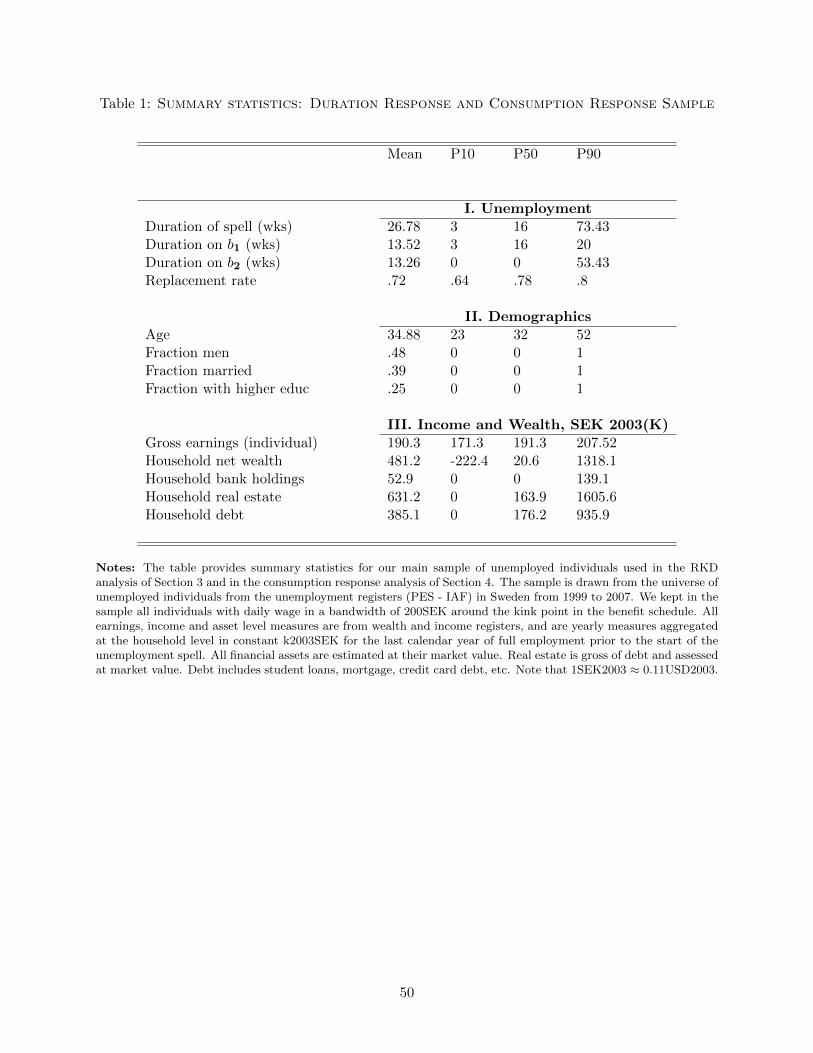
Table 1: Summary statistics: Duration Response and Consumption Response Sample
Mean P10 P50 P90
I. UnemploymentDuration of spell (wks) 26.78 3 16 73.43Duration on b1 (wks) 13.52 3 16 20Duration on b2 (wks) 13.26 0 0 53.43Replacement rate .72 .64 .78 .8
II. DemographicsAge 34.88 23 32 52Fraction men .48 0 0 1Fraction married .39 0 0 1Fraction with higher educ .25 0 0 1
III. Income and Wealth, SEK 2003(K)Gross earnings (individual) 190.3 171.3 191.3 207.52Household net wealth 481.2 -222.4 20.6 1318.1Household bank holdings 52.9 0 0 139.1Household real estate 631.2 0 163.9 1605.6Household debt 385.1 0 176.2 935.9
Notes: The table provides summary statistics for our main sample of unemployed individuals used in the RKDanalysis of Section 3 and in the consumption response analysis of Section 4. The sample is drawn from the universe ofunemployed individuals from the unemployment registers (PES - IAF) in Sweden from 1999 to 2007. We kept in thesample all individuals with daily wage in a bandwidth of 200SEK around the kink point in the benefit schedule. Allearnings, income and asset level measures are from wealth and income registers, and are yearly measures aggregatedat the household level in constant k2003SEK for the last calendar year of full employment prior to the start of theunemployment spell. All financial assets are estimated at their market value. Real estate is gross of debt and assessedat market value. Debt includes student loans, mortgage, credit card debt, etc. Note that 1SEK2003 ≈ 0.11USD2003.
50

Table 2: RKD estimates at the 725SEK threshold
(1) (2) (3)Unemployment Duration D1 Duration D2
Duration D (< 20 weeks) (≥ 20 weeks)
I. 1999-2000: Kink in b1 and b2δk -.0569 -.0246 -.0299
(.0050) (.0012) (.0039)εDk,b
1.530 1.319 1.615
(.1300) (.0645) (.1986)N 187518 187518 187518
II. 2001: Kink in b2 onlyδk -.0255 -.0115 -.0105
(.0049) (.0020) (.0030)εDk,b2 .6765 .6015 .5921
(.1312) (.1061) (.1642)N 65545 65545 65545
III. 2002-. : Placeboδk .0045 -.0016 .006
(.0055) (.0011) (.0049)N 172645 172645 172645
IV. Moral Hazard Estimates
MH = b+τb· εD,b 1.637 (.1391)
MH2 = b+τb· DD2
· εD,b2 1.445 (.2829)
MH1 = b+τb· DD1
· (εD,b − εD,b2) 1.819 (.4032)
Hypotheses testing : MH1 = MH2 z-stat p-value
Z-test -0.57 0.569Permutation Test 0.059
Notes: The table reports estimates of the change in slope δk, at the 725SEK threshold, in the relationship betweendaily wage and the total duration of unemployment D (col. (1)), the time D1 spent on the first part of the SwedishUI profile (col. (2)) and the time D2 spent on the second part of the Swedish UI profile (col. (3)). Estimates areobtained from linear regressions of the form of equation (16) with a bandwidth size h = 90SEK. Panel I reportsestimates for spells starting before July 2001. Panel II reports estimates for spells starting after July 2001 and beforeJuly 2002. Panel III reports estimates for spells starting after July 2002. Unemployment duration is capped at twoyears. We report implied elasticities, computed as εDk,bk = δk · wk
Dcapb
, where δk is the estimated marginal slope
change, and Dcapb is the observed average duration at the kink. In Panel IV we also report implied moral hazard costs
estimates defined in equation (6). MH is the moral hazard cost of increasing benefits throughout the unemploymentspell. MH1 is the moral hazard cost of increasing benefits given for the first 20 weeks of the spell. MH2 is the moralhazard cost of increasing benefits given after the first 20 weeks of the spell. Computations assume τ = .05 whichbalances the UI budget on average during the period 1999-2007. It follows that b+τ
b= 1 + .05/.72 = 1.07. See text
for details. Standard errors are obtained from bootstrapping using 50 replications.
51

Table 3: Welfare evaluation of actual profile using estimated sufficient statistics
(1) (2) (3) (4) (5) (6)Moral hazard Average Consumption Benefit-
hazard consumption smoothing gains Costcosts drop CSk ratio
MHk ∆ck γ = 1 γ = 2 γ = 5 CSk/MHk
Benefits given 1.64 .08 .08 .16 .40 γ × .049throughout the spell: b (.14) (.01) (.01) (.02) (.04)
Benefits given 1.82 .05 .05 .10 .24 γ × .026for the first 20 weeks: b1 (.40) (.01) (.01) (.02) (.04)
Benefits given 1.45 .10 .10 .19 .48 γ × .066after first 20 weeks: b2 (.28) (.02) (.02) (.03) (.08)
Notes: The Table reports estimates of the sufficient statistics needed to evaluate the benefit profile in place inSweden. The first row analyzes the welfare consequences of an increase in benefits b throughout the unemploymentspell. The second row analyzes the welfare consequences of an increase in benefits b1 during the first 20 weeks of theunemployment spell. The third row analyzes the welfare consequences of an increase in benefits b2 after 20 weeks ofunemployment. In each case, column (1) repeats our estimates of the moral hazard cost of an increase in benefits(Panel IV of Table 2). The second column repeats our estimates of the average consumption drop (column 1 of TableC-3). To estimate the average consumption drop over the entire spell, we run the same regression as in (29) but withonly one dummy 1[t > 0] that indicates being observed while unemployed. We convert the respective consumptiondrops into estimates of the consumption smoothing gains CSk, following the implementation in (14), which relies ona Taylor approximation and homogeneous preferences. The consumption smoothing gains are reported for a rangeof plausible values of the relative risk aversion γ in columns (3) to (5). Column (6) shows the ratio of consumptionsmoothing gains to moral hazard costs, CSk/MHk, depending on the uniform relative risk aversion γ. This ratiocorresponds to the marginal value of a (tax-funded) kroner spent on unemployment benefits, accounting for theunemployment responses. Bootstrapped standard errors in parentheses.
52

FOR ONLINE PUBLICATION - Appendix A: Technical Appendix
This Appendix provides the technical details of our model setup and the proofs of the Propositions. We also consider
extensions of the baseline model to gauge the robustness of our characterization of the optimal benefit profile. We
finally compare the evolution of consumption smoothing gains and moral hazard in stationary and non-stationary
environments.
A.1 Setup
We closely follow the setup in Chetty [2006], but allow for heterogeneous agents and non-stationarities. Let ωi,t denote
a vector of state variables that contain all relevant information up to time t in determining an agent i’s employment
status and behavior at time t. Let Fi,t (ωi,t) denote the unconditional distribution of ωi,t given information available
at time 0. We assume that Fi,t is a smooth function and let Ω denote the maximal support of Fi,t for ∀i,∀t. In our
stylized model, the vector of state variables ωi,t includes only the asset level, time and the employment status.
In each period t, an agent decides how much to consume from her income and assets. In our stylized model, an
agent earns w − τ when employed and receives b when unemployed. The law of motion of assets in the employment
and unemployment state are respectively,
ai,t+1 = rai,t + w − τ − cei,t (22)
ai,t+1 = rai,t + bt − cui,t, (23)
but are constrained to be above ai,t+1 ≥ ai for each agent i and any time t. We denote the Lagrange multipliers on
these constraints by µei,t (ωi,t) , µui,t (ωi,t) and µai,t (ωi,t) respectively.
Let θi,t (ωi,t) denote an agent’s employment status at time t in state ωi,t. If θ = 1, the agent is employed, and
if θ = 0, the agent is unemployed. In each period t, an unemployed agent chooses a level of search effort si,t as
well. This search effort level determines the probability to leave unemployment for employment in that period. This
mapping may be agent-specific and change depending on the length of the unemployment spell.
Each agent i chooses a program (si, cui , c
ei ) with
si = si,t (ωi,t)t∈1,2,..T,ωi,t∈Ω,θ(ωi,t)=0 ,
cui =cui,t (ωi,t)
t∈1,2,..T,ωi,t∈Ω,θ(ωi,t)=0
,
cei =cei,t (ωi,t)
t∈1,2,..T,ωi,t∈Ω,θ(ωi,t)=1
,
to solve
Vi (P ) = max ΣTt=1βt−1
∫vui
(cui,t (ωi,t) , si,t (ωi,t)
)[1− θi,t (ωi,t)] + vei
(cei,t (ωi,t)
)θi,t (ωi,t)dFi,t (ωi,t)
+ ΣTt=1βt−1
∫µui,t (ωi,t)
[rai,t (ωi,t−1) + bt − cui,t (ωi,t)− ai,t+1 (ωi,t)
][1− θi,t (ωi,t)] dFi,t (ωi,t)
+ ΣTt=1βt−1
∫µei,t (ωi,t)
[rai,t (ωi,t−1) + w − τ − cei,t (ωi,t)− ai,t+1 (ωi,t)
]θi,t (ωi,t) dFi,t (ωi,t)
+ ΣTt=1βt−1
∫µai,t (ωi,t) [ai − ai,t+1 (ωi,t)] dFi,t (ωi,t) ,
where we use the short-hand notation ωi,t−1 to denote the vector of state variables at time t − 1 that preceded the
vector of state variables ωi,t at time t. Following Chetty [2006], we assume that lifetime utility is smooth, increasing
and strictly quasi-concave in (cui , cei , si) and that the value function Vi (P ) is differentiable such that the Envelope
53

Theorem applies. This implies that
∂Vi (P )
∂bt= βt−1
∫µui,t (ωi,t) [1− θi,t (ωi,t)] dFi,t (ωi,t)
= βt−1
∫∂vui
(cui,t (ωi,t) , si,t (ωi,t)
)∂cui,t
[1− θi,t (ωi,t)] dFi,t (ωi,t) .
The second equality uses the optimality of the consumption choice cui,t (ωi,t), which does not depend on the borrowing
constraint being binding or not.
In our stylized model, the agent starts unemployed and remains employed until T once she finds a job. The
agent’s exit rate out of unemployment at time t only depends on her search effort at time t. The (unconditional)
probability to be unemployed at time t+ 1 therefore simplifies to
Pr (θi,t+1 = 0) =
∫(1− hi,t (si,t (ωi,t))) [1− θi,t (ωi,t)] dFi,t (ωi,t) .
This simplifying assumption makes that on the optimal path an agent’s unemployment consumption cui,t (ωi,t) only
varies with time t, which coincides with the number of periods she is currently unemployed. The agent’s employment
consumption cei,t (ωi,t), however, depends on both time t and the number of periods she has been unemployed.
We now turn to the policy. We can express the present value of the government’s budget as
G (P ) = ΣTt=1 [1 + r]−(t−1)
∫ ∫−bt [1− θi,t (ωi,t)] + τθi,t (ωi,t)dFi,t (ωi,t) di,
which simplifies to (1) when r = 0.
The government solves
max
∫Vi (P ) di+ λ
[G (P )− G
],
where λ is the Lagrange multiplier on the government’s budget constraint and G is an exogenous revenue constraint.
Our characterization is based on local policy changes and thus only allows for local tests and recommendations. For
the local recommendations to translate globally, we would need the program to be strictly concave in P .62 To provide
tractable expressions of the local welfare implications we assume that the social welfare function is differentiable.
A.2 Dynamic Unemployment Policy
A.2.1 Proof of Proposition 1
The welfare impact of a change in benefit level bt of policy P equals
∂W (P )
∂bt=
∫∂Vi (P )
∂btdi+ λ
∂G (P )
∂bt,
where, using Srt ≡ St/ [1 + r](t−1) and εrt′,t =∂Srt′
∂bt
btSrt′,
∂G (P )
∂bt= −Srt − ΣTt′=1 (bt′ + τ)
∂Srt′
∂bt= −Srt ×
[1 + ΣTt′=1
Srt′ (bt′ + τ)
Srt btεrt′,t
],
62Chetty (2006) provides regularity conditions such that the government’s problem is strictly concave in case offlat unemployment policies (i.e., bk = b).
54

which simplifies to expression (5) for r = 0, and∫∂Vi (P )
∂btdi =
∫ ∫βt−1 ∂v
ui
(cui,t (ωi,t) , si,t (ωi,t)
)∂cui,t
[1− θi,t (ωi,t)] dFi,t (ωi,t)di
= βt−1StE
(∂vui
(cui,t (ωi,t) , si,t (ωi,t)
)∂cui,t
|t, θi,t (ωi,t) = 0
).
This expression simplifies to (7) for β = 1 + r = 1. The expectation operator Eut (·) thus averages over all potential
states in which the agent is unemployed at time t. In our stylized setup (which assumes that the agent starts unem-
ployed and remains employed once she finds a job), the agent’s unemployment consumption cui,t (ωi,t) only depends
on the length of the ongoing unemployment spell. The weight of agent i’s marginal utility in calculating the average
marginal utility among the unemployed at time t is scaled by Si,t/St.
Combining the two expressions, we find
∂W (P )
∂bt= 0⇔
∫ ∂Vi(P )∂bt
di− λλ
= ΣTt′=1
Srt′ (bt′ + τ)
Srt btεrt′,t.
In the same way, we find
∂G (P )
∂τ=[ΣTt=1 (1− St) / [1 + r](t−1)
]×
[1 + ΣTt′=1
Srt′ (bt′ + τ)
ΣTt=1(1− St) / [1 + r](t−1)τεrt′,τ
],
∫∂Vi (P )
∂τdi = ΣTt=1β
t−1 (1− St)E
(∂vei
(cei,t (ωi,t)
)∂cei,t
|t, θi,t (ωi,t) = 1
),
and, hence,∂W (P )
∂τ= 0⇔ λ−
∫ ∂Vi(P )∂τ
di
λ= ΣTt′=1
Srt′ (bt′ + τ)
ΣTt=1(1− St) / [1 + r](t−1)τεrt′,τ ,
which simplifies to expression (9) for β = 1 + r = 1, with (T −D) equal to the expected time spent employed
ΣTt=1 (1− St). The expectation operator Ee (·) in (9) is over all employment states and periods t. Compared to
consumption during unemployment, employment consumption cei,t (ωi,t) depends on the unemployment history and
not just on time t. Hence, we need to calculate the average marginal utility when employed at time t for any agent i
and scale the weight in calculating the average marginal utility among the employed at time t by (1− Si,t) / (1− St).
We then average over all periods t using weights (1− St) / (T −D).
The n + 1 first-order conditions stated in the Proposition, jointly with the budget constraint, are necessary con-
sidtions for an interior, optimal policy.
A.2.2 Robustness of Characterization
We briefly show how the optimal tax formulae continue to apply in a model with multiple unemployment spells where
an agent i’s layoff probability li (ei,t) at time t depends on her effort on the job ei,t. We still assume that ωi,t contains
all relevant information up to time t in determining an agent i’s employment status and behavior at time t. Let
θi,t (ωi,t) still denote an agent’s employment status at time t in state ωi,t. If θ = 1, the agent is employed, and if
θ = 0, the agent is unemployed.
From the consumption smoothing perspective, the agent’s marginal utility when employed can now depend on the
effort on the job, ∂vei(cei,t (ωi,t) , ei,t (ωi,t)
)/∂cei,t. From the moral hazard perspective, the (unconditional) probability
55

to be unemployed now equals
Pr (θi,t+1 = 0) =
∫(1− hi (si,t (ωi,t) , ωi,t)) [1− θi,t (ωi,t)] + li (ei,t(ωi,t)) θi,t (ωi,t) dFi,t (ωi,t) .
We introduce the indicator functions I ti,t (ωi,t) which take value 1 if the length of the ongoing unemployment spell
equals t and 0 otherwise. Hence,
Pr(I1i,t+1 = 1
)=
∫li (ei,t(ωi,t)) θi,t (ωi,t) dFi,t (ωi,t) ,
Pr(I ti,t+1 = 1
)=
∫(1− hi (si,t (ωi,t) , ωi,t))I
t−1i,t (ωi,t) dFi,t (ωi,t) .
The budget constraint still depends on the survival rate at each unemployment duration Srt , but now potentially
spread over multiple spells. That is,
Srt = ΣTt=1 [1 + r]−(t−1)
∫ ∫I ti,t (ωi,t) dFi,t (ωi,t) di.
Hence, the optimal formulae in Proposition 1 remain exactly the same (with the marginal utility of consumption
when employed depending on effort on the job). The policy-relevant elasticity should account for potential responses
in the layoff rate to a change in the unemployment policy. In our context, however, we find no significant responses
in the layoff rates to changes in UI benefits.63
We refer to Chetty [2006] for a detailed treatment of other extensions of the model (including private insurance
arrangements, spousal labour supply, etc.) which do not affect the optimal tax formulae due to envelope conditions.
This remains true when extending his analysis to a dynamic benefit profile. For example, we can introduce alternative
sources of income zi,t (xi,t, ωi,t) into the agent’s budget constraints (22) and/or (23), with the income level depending
on the agent’s choice variable xi,t, which may enter the agent’s utility function when employed and/or unemployed.
As long as there are no externalities related to this alternative source of income, envelope conditions imply that the
welfare impact of a policy change is still captured by the same statistics.
A.2.3 Characterization with Employer Screening
We consider a reduced-form model of employer screening based on Lockwood [1991] and Lehr [2017]. The job finding
rate rate hi,t (si,t,St) = λi (si,t)×µt(St) is determined not only by the probability that agent i finds a vacant position
λi (si,t), depending on her own search effort, but also by the probability that the matching firm hires the agent µt(St)
where St = Si′,ti′ . The hiring probability at time t depends on the relative survival rates by agents with different
productivity. In a two-type version of the model (H and L), where an agent i’s type affects both her productivity θi
and the probability of finding a vacancy λi (si,t), the firm’s optimal hiring rate when matched with a job seeker who
has been unemployed for t periods increases in the relative survival rate of the high type at time t. In particular, if
the firm’s profit of hiring an agent equals θi−w, where θH > θL = 0, the firm’s optimal hiring decision equals µt = 1
63First, if layoff rates respond to the unemployment policy, this has implications regarding the pdf of daily wagesaround the kink in our empirical setting. The presence of a kink in benefits should create bunching at the kink ifthere is moral hazard on the job with convex costs of shirking. We show in subsection B.4 of Appendix B that wecannot detect any bunching at the kink. Furthermore, if layoffs are responsive to UI benefits this should also affectthe pdf of daily wages when the kink in the schedule is removed. We show in subsection B.4 of Appendix B thatwe cannot detect such changes in the pdf of daily wages after the removal of the kinks in the schedule. While thisevidence is far from definitive, it suggests that layoff rates do not seem to strongly respond to UI benefits in ourcontext.
56

ifSHtSLtθH ≥ w and 0 otherwise. As a consequence, with the more productive type leaving unemployment at a faster
rate, the firm would not hire job seekers who have been unemployed for longer than t whereSHtSLt
θH = w.
In the employer screening model, an agent’s search effort will affect the job finding probability of any other
agent, positively or negatively depending on her type, but no agent internalizes this effect. For simplicity we focus
on job seekers’ welfare and ignore the impact on firms’ profits. Note that the setup can in principle also encompass
richer models with rationing (e.g., Michaillat [2012b]) and employer ranking (e.g., Blanchard and Diamond [1994]),
in which job seekers’ search effort crowd out the job finding rate of other job seekers. This is analyzed in Landais
et al. [2010] who account for firms’ profits and labor-demand behavior more generally and show how the distinction
between micro and macro elasticities becomes relevant for the characterization of the optimal (static) unemployment
policy in general equilibrium.
The impact of a policy change on the agents’ welfare equals∫∂Vi (P )
∂btdi =
∫Si,t
∂vui (cui,t,si,t)∂cui,t
di+ Σ∞t′=1[
∫Si,t′λi (si,t′)
∂µt′∂St′
∂St′∂bt
βt′ [V ei,t′ − V ui,t′
]di]
= λSt[1 + CSt] + Σ∞t′=1
St′
St[
∫Si,t′
St′
∂λi(si,t′)µt′∂St′
∂St′∂bt
βt′ [V ei,t′ − V ui,t′
]/λdi]
≡ λSt
[1 + CSt] + Σ∞t′=1
St′
StEut′
(∂ht′
∂btωht′
).
We can correct the moral hazard cost for this new externality so that
∂W (P )
∂bt= λSt × [CSt −MHx
t ] ,
with
MHxt ≡ ΣTt′=1
St′
St
[bt′ + τ
btεt′,t − Eut′
(ωht′
∂ht′
∂bt
)],
The welfare impact of an increase in the exit rate rate is positive, ωhi,t′ = βt′ [V ei,t′ − V ui,t′
]/λ. The change in the exit
rate ∂ht′/∂bt (through the change in hiring) will depend on the change in the relative survival rates at time t′ in
response to the change in benefits at time t. This corresponds to the correction proposed by Lehr [2017] for a flat
benefit profile. A change in the unemployment policy won’t change hiring, if the survival rate response of types with
different productivity responds is the same. That is, εit′,t = εi′
t′,t.
Embedding this in our framework allows to assess the impact on the benefit profile as well. For the hiring
externatity to change the gradient of the moral hazard costs, we need a change in the benefit level bt to cause a
different response in the relative survival rate (scaled by 1/St) depending on the timing of the change. In our stylized
two-type example the response in relative survival rate SHt /SLt at the threshold duration t determines whether
hiring increases or decreases. Indeed, the firm will hire job seekers with longer unemployment duration than t if the
productive type is more responsive than the less productive type to a change in bt, i.e., εHt,t > εLt,t . The externality
response would be positive and thus causes MHxt < MHt. In the model with heterogeneity in the returns to search,
discussed in subsection 5.2.1 and considered below, we show that εit,t can be increasing in the return to search for
benefit levels paid early in the spell, but at the same decreasing for benefit levels paid late in the spell. Intuitively,
the increase in the returns to search reduces the survival rate into longer unemployment spells and thus reduces the
responsiveness to changes in benefits timed later on. Hence, with heterogeneity in the returns to search, the gradient
of the moral hazard cost could become steeper when adjusted for the hiring externality.
57
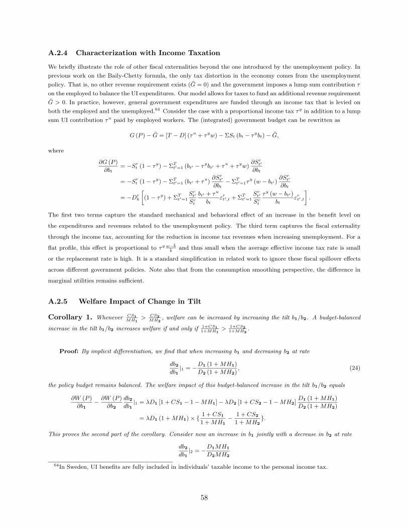
A.2.4 Characterization with Income Taxation
We briefly illustrate the role of other fiscal externalities beyond the one introduced by the unemployment policy. In
previous work on the Baily-Chetty formula, the only tax distortion in the economy comes from the unemployment
policy. That is, no other revenue requirement exists (G = 0) and the government imposes a lump sum contribution τ
on the employed to balance the UI expenditures. Our model allows for taxes to fund an additional revenue requirement
G > 0. In practice, however, general government expenditures are funded through an income tax that is levied on
both the employed and the unemployed.64 Consider the case with a proportional income tax τy in addition to a lump
sum UI contribution τu paid by employed workers. The (integrated) government budget can be rewritten as
G (P )− G = [T −D] (τu + τyw)− ΣSt (bt − τybt)− G,
where
∂G (P )
∂bt= −Srt (1− τy)− ΣTt′=1 (bt′ − τybt′ + τu + τyw)
∂Srt′
∂bt
= −Srt (1− τy)− ΣTt′=1 (bt′ + τu)∂Srt′
∂bt− ΣTt′=1τ
y (w − bt′)∂Srt′
∂bt
= −Drk
[(1− τy) + ΣTt′=1
Srt′
Srt
bt′ + τu
btεrt′,t + ΣTt′=1
Srt′
Srt
τy (w − bt′)bt
εrt′,t
].
The first two terms capture the standard mechanical and behavioral effect of an increase in the benefit level on
the expenditures and revenues related to the unemployment policy. The third term captures the fiscal externality
through the income tax, accounting for the reduction in income tax revenues when increasing unemployment. For a
flat profile, this effect is proportional to τy w−bb
and thus small when the average effective income tax rate is small
or the replacement rate is high. It is a standard simplification in related work to ignore these fiscal spillover effects
across different government policies. Note also that from the consumption smoothing perspective, the difference in
marginal utilities remains sufficient.
A.2.5 Welfare Impact of Change in Tilt
Corollary 1. Whenever CS1MH1
> CS2MH2
, welfare can be increased by increasing the tilt b1/b2. A budget-balanced
increase in the tilt b1/b2 increases welfare if and only if 1+CS11+MH1
> 1+CS21+MH2
.
Proof: By implicit differentiation, we find that when increasing b1 and decreasing b2 at rate
db2db1|1 = −D1 (1 +MH1)
D2 (1 +MH2), (24)
the policy budget remains balanced. The welfare impact of this budget-balanced increase in the tilt b1/b2 equals
∂W (P )
∂b1− ∂W (P )
∂b2
db2db1|1 = λD1 [1 + CS1 − 1−MH1]− λD2 [1 + CS2 − 1−MH2]
D1 (1 +MH1)
D2 (1 +MH2)
= λD1 (1 +MH1)× 1 + CS1
1 +MH1− 1 + CS2
1 +MH2.
This proves the second part of the corollary. Consider now an increase in b1 jointly with a decrease in b2 at rate
db2db1|2 = −D1MH1
D2MH2
64In Sweden, UI benefits are fully included in individuals’ taxable income to the personal income tax.
58

The welfare impact of such increase in the tilt b1/b2 equals
∂W (P )
∂b1− ∂W (P )
∂b2
db2db1|2 = λD1 [CS1 −MH1]− λD2 [CS2 −MH2]
D1MH1
D2MH2
= λD1MH1 ×CS1
MH1− CS2
MH2
.
Hence, whenever CS1/MH1 exceeds CS2/MH2, such increase in the tilt b1/b2 increases welfare and vice versa.
A.3 Dynamic Sufficient Statistics in Stationary Environment
A.3.1 Proof of Proposition 2
We consider a flat benefit profile bt = b < w − τ for ∀t in a single-type, stationary environment hi,t (·) = h (·) for
∀i, t. We also assume β (1 + r) = 1 and T =∞. We compare the impact of an increase in the benefit level at time t
and at time t+ 1.
We analyze first the moral hazard costs. We assume that the agent is borrowing constrained and thus consumes
hand-to-mouth when unemployed and employed ( cut = bt and cet = w−τ). This set up follows Hopenhayn and Nicolini
[1997]. Using notation Srt = (1 + r)−(t−1) St, we find
∂G (P )
∂bt= −Srt − ΣTj=1 (bj + τ)
∂Srj∂bk
= −Srt × [1 +b+ τ
b
Dr
SrtεDr,bt ].
For an increase in bt+1, we find
∂G (P )
∂bt+1= −Srt+1 × [1 +
b+ τ
b
Dr
Srt+1
εDr,bt+1 ].
Using
Dr = ΣTj=1Srj = 1 +Dr
2 = 1 + Sr2Dr2,
where Dr2 = ΣTj=2S
rj and Dr
2 =[ΣTj=2S
rj /S
r2
], we can write
εDr,bt+1 =∂ [1 +Dr
2]
∂bt+1
b
Dr=
∂Dr2
∂bt+1
b
Dr2
Dr2
Dr
=[εSr2 ,bt+1 + εDr2,bt+1
] Dr2
Dr.
Since the environment is stationary and the agent is borrowing-constrained, the agent’s search behavior remains the
same over the unemployment spell (conditional on the continuation policy being the same). Starting from a flat
profile, an increase in bt has the same impact on the continuation policy evaluated at time 1 as an increase in bt+1
has on the continuation policy evaluated at time 2, conditional on being still unemployed then. The impact of the
policy changes at time t and t+ 1 on the remaining duration at time 1 and time 2 respectively is the same. Hence,
we have εDr2,bt+1= εDr,bt for T = ∞. Denoting the constant exit rate for the flat profile by h, we have Dr = 1+r
r+h
and Dr2 = 1−h
1+r1+rr+h
, while Srt+1 = 1−h1+r
Srt . This implies
Dr2
Srt+1
=Dr
Srt.
59

Using this equality and the expression for εDr,bt+1 , we can re-write
∂G (P )
∂bt+1= −Srt+1 × [1 +
b+ τ
b
Dr
Srt+1
εDr,bt+1 ]
= −Srt+1 × [1 +b+ τ
b
Dr2
Srt+1
[εSr2 ,bt+1 + εDr,bt
]]
= −Srt+1 × [1 +b+ τ
b
Dr
Srt
[εSr2 ,bt+1 + εDr,bt
]].
This implies that
MHt+1 =b+ τ
b
Dr
SrtεSr2 ,bt+1 +
b+ τ
b
Dr
SrtεDr,bt ≥MHt,
since εSr2 ,bt+1 ≥ 0. Starting from a flat profile, the moral hazard cost is thus higher for any benefit increase that is
timed later during the spell.
We now analyze the consumption smoothing gains. In our stylized setup (which assumes that the agent starts
unemployed and remains employed once she finds a job), an optimizing agent’s unemployment consumption cut (ωt)
(and search effort st (ωt)) only depends on the length of the ongoing unemployment spell. Hence, we have∫∂Vi (P )
∂btdi = βt−1St
∂vu (cut , st)
∂cut.
When the agent is borrowing constrained, the agent is hand-to-mouth cut = bt and the marginal utility of consumption
(and thus CSt) remains constant for a flat benefit profile. When not borrowing constrained, an agent who is unem-
ployed at time t increases her consumption by depleting her assets to equalize the marginal utility of consumption
at time t with the expected marginal utility of consumption at t + 1. The unemployment consumption level cut at
time t, the consumption level upon finding employment cet+1 at time t+ 1 and the consumption level when still being
unemployed cut+1 at time t+ 1 satisfy a standard Euler condition,
∂vu (cut , st)
∂cut= ht (st)
∂ve (cet+1)
∂cet+1
+ (1− ht (st))∂vu (cut+1, st+1)
∂cut+1
for β (1 + r) = 1. With separable concave preferences, ∂vu (c, s) /∂c = ∂ve (c) /∂c = v′ (c) ,and, benefits lower than
the after-tax wage b < w − τ , for any given asset level, an agent has higher expected lifetime income when employed
than when unemployed. The marginal value of an increase in assets is lower when employed than when unemployed,
i.e., ∂V et+1/∂at+1 < ∂V ut+1/∂at+1. This implies the marginal utility of consumption is lower when employed than
when unemployed at t + 1. Hence, by the Euler condition, v′ (cut+1) > v′ (cet+1) implies v′ (cut+1) > v′ (cut ). On the
optimal path, the marginal utility of consumption is increasing over the spell and the consumption gains are thus
always higher for benefits timed later during the unemployment spell.
The stationary forces and how they affect the optimal benefit profile are well known in the literature and
arguably robust. Our set up with the borrowing-constrained agent follows Hopenhayn and Nicolini [1997]. The
assumption that the agent is borrowing constrained is restrictive, but guarantees that search behaviour remains
the same over the unemployment spell and thus simplifies the derivations. Note that search behaviour remains
the same in a model with savings when the agent has CARA preferences with monetary cost of search efforts (i.e.,
vu (c, s) = − exp (−σ [c− ψ (s)]) as in Spinnewijn [2015], again simplifying the derivation of the optimal benefit profile.
It is also clear from the proof that relaxing the borrowing constraint would not change the conclusion regarding the
gradient of the moral hazard costs when εDr2,bt+1≥ εDr,bt and ht+1 ≥ ht (so that
Dr2Srt+1
> Dr
Srt) for any t. We analyze
this further for a specific search environment with non-stationary features. The result that the marginal utility of
consumption is increasing over the spell continues to hold for unconstrained job seekers when the benefit profile is
not flat but bt < w − τ for all t. The assumption that the agent’s preferences are separable is also more restrictive
than necessary. The proof highlights that it suffices for the marginal value of an increase in assets to be lower when
employed than when unemployed.
60

A.4 Dynamic Sufficient Statistics in a Non-stationary Environment
We now specify particular functions for the search environment and introduce non-stationary features in our model.
We allow for depreciation in search efficacy, heterogeneity in search efficacy, and heterogeneity in assets. We study
how these forces affect the predicted increase in MHt and CSt throughout the unemployment spell from Proposition
2. We allow for all these non-stationary forces simultaneously in our structural model in Appendix D.
We establish three results: (i) in a model with depreciation in the return-to-search parameter (i.e., ht (si,t) =
h0 + θth1sρi,t), the moral hazard cost cost of benefit changes that start later in the spell can be arbitrarily close to
the moral hazard cost of benefit changes that start earlier, (ii) in a model with heterogeneity in the return-to-search
parameter (i.e., ht (si,t) = h0 +hi1sρi,t), the moral hazard costs can actually be lower for benefit changes timed later in
the spell,, (iii) in a model with asset heterogeneity, negatively correlated with exit rates, the consumption smoothing
gains can actually be higher earlier in the spell.
A.4.1 Preliminaries
For our analysis of moral hazard costs, we assume that agents are borrowing constrained throughout the unemploy-
ment spell (i.e., unemployment consumption equals UI benefits), that preferences are separable in consumption and
search, u (c, s) = u (c)− s, and that the exit rate function has the following form,
h (si,t) = h0 + h1sρi,t for ∀i, t.
For tractability, we assume that the optimal search effort is interior and thus the resulting exit rate is between 0 and
1.
Each individual has a value function for the employed and unemployed state shown below:
V ei,t = u(w − τ) + βV ei,t+1
V ui,t = u(bt)− si,t + βhi,t (si,t) [V ei,t+1 − V ui,t+1] + βV ui,t+1,
Since the employment state is absorbing, we have V et = u(w−τ)1−β .The optimal level of effort equals
si,t = (ρβh1,i,t[Vei,t+1 − V ui,t+1])
11−ρ .
We start from a flat benefit profile and compare a permanent benefit rise in t = 2 (denoted by b2→∞) and in
t = 3 (denoted by b3→∞) respectively. Note that t = 1 is the first period that an agent exerts effort, but this is
unaffected by the benefit level b1. The moral hazard cost of raising benefits permanently in period t, starting from a
flat profile, is given by:
MHt→∞ =
∂Dr
∂bt→∞
Drt→∞
(b+ τ) .
To save on notation we consider instead D =∑∞t′=1 St′ and Dt→∞ =
∑∞t′=t St′ , corresponding to Dr and Dr
t→∞ for
r = 0, but we make sure our conclusions are robust to β → 1.
A.4.2 Stationary Environment
We first confirm that for this specific search environment, in the absence of non-stationary features, the moral hazard
cost of increasing the UI benefits is always higher when this increase is timed later in the spell, in line with Proposition
2. This will help highlighting why non-stationary features can affect this result.
Consider first an increase in b2→∞. In this scenario, we have that V ut = V ut+1 = V u2 if t ≥ 2. As a result we have
61

only two value functions when unemployed:
V U1 = u(b)− s+ β(h0 + h1sρ)[V e − V u2 ] + βV u2
V u2 = u(b2→∞)− s+ β(h0 + h1sρ)[V e − V u2 ] + βV u2
and one level of effort:
s = (ρβh1[V e − V u2 ])1
1−ρ .
Hence, we can write
St = (1− h0 − h1sρ)t−1,
D =1
h0 + h1sρ
D2→∞ =1− h0 − h1s
ρ
h0 + h1sρ
Since we evaluate the benefit change for a flat profile, we will use the fact that before differentation V u1 = V u2 = V u.
We calculate the effect of the benefit rise on the average unemployment duration, which in turn depends on the
change in effort, which in turn depends on the change in the value of being unemployed:
∂D
∂b2→∞= −
ρh1sρ−1 ∂s
∂b2→∞
(h0 + h1sρ)2,
∂s
∂b2→∞= − s
1− ρ [V e − V u]−1 ∂V u2∂b2→∞
,
∂V u2∂b2→∞
=u′(·)
1− β(1− h0 − h1sρ).
Consider now an increase in b3→∞. Note that V ut = V ut+1 = V U3 if t ≥ 3. Therefore, there are only three value
functions when unemployed:
V u1 = u(b)− s1 + β(h0 + h1sρ1)[V e − V u2 ] + βV u2
V u2 = u(b)− s2 + β(h0 + h1sρ2)[V e − V u3 ] + βV u3
(1− β)V U3 = u(b3→∞)− s2 + β(h0 + h1sρ2)[V e − V u3 ],
and two levels of effort:
s1 = (ρβh1[V e − V u2 ])1
1−ρ
s2 = (ρβh1[V e − V u3 ])1
1−ρ .
Similar to before, we find
∂D
∂b3→∞=−ρh1s
ρ−1 ∂s1∂b3→∞
(h0 + h1sρ)− ρh1s
ρ−1 ∂s2∂b3→∞
(1− h0 − h1sρ)
(h0 + h1sρ)2,
which is composed of the following derivatives:
∂s1
∂b3→∞= − s
1− ρ [V e − V u]−1 ∂V u2∂b3→∞
∂s2
∂b3→∞= − s
1− ρ [V e − V u]−1 ∂V u3∂b3→∞
,
62

which are, in turn, composed of the following derivatives:
∂V U3∂b3→∞
=u′(·)
1− β(1− h0 − h1sρ),
∂V U2∂b3→∞
= −β(h0 + h1sρ)
∂V u3∂b3→∞
+ β∂V u3∂b3→∞
.
Putting everything together, we find for b2→∞ and b3→∞:
∂D
∂b3→∞=
∂D
∂b2→∞(1− h0 − h1s
ρ)[1 + β(h0 + h1sρ)],
while
D3→∞ = D2→∞(1− h0 − h1sρ).
The impact of an increase in b3→∞ on the time spent unemployed is smaller than the impact of an increase in b2→∞,
since a smaller part of the unemployment policy is affected, as captured by the scalar [1 − h0 − h1sρ] in the both
expressions above, for the duration responses and the durations respectively. However, while the increase in b3→∞
starts later, it will reduce the exit rates earlier in the spell as well, as captured by the scalar [1 + β(h0 + h1sρ)] in
the expression for the duration responses. These are the forward-looking incentives identified before in Shavell and
Weiss [1979]. Indeed, in line with Proposition 2, we find
MH2→∞
MH3→∞=
1
1 + β(h0 + h1sρ)< 1.
This intuition generalizes for any changes bt→∞ and bt+1→∞ respectively and is robust to β → 1.
A.4.3 Depreciation in Search Efficacy
We now assume that the returns to search depreciate at a geometric rate,
ht (si,t) = h0 + θt−1h1sρi,t = θt−1hsρi,t for θ ∈ [0, 1] .
To simplify the expressions below, we assume that the exit rate is zero when no search is exerted (i.e., h0 = 0), but
the argument below continues to apply when relaxing this assumption. From the value of being unemployed at time
t and the effort level at time t, we can derive the following derivatives:
∂V ut∂bt→∞
= β(1− hθt−1sρt )∂V ut+1
∂bt→∞∀ 0 < t < t
∂V ut∂bt→∞
= u′ (b) + β(1− hθt−1sρt )∂V ut+1
∂bt→∞∀ t ≥ t
∂st∂bt→∞
=−st
1− ρ [V e − V ut+1]−1 ∂Vut+1
∂bt→∞,
which can be used in order to derive an expression for the derivative of the average unemployment duration:
∂D
∂bt→∞=
∂
∂bt→∞[1 + (1− hsρ1) + (1− hsρ1)(1− hθsρ2) + (1− hsρ1)(1− hθsρ2)(1− hθ2sρ3) + . . .]
= −ρh[sρ−1
1
∂s1
∂bt→∞
D2→∞
1− hsρ1+ θsρ−1
2
∂s2
∂bt→∞
D3→∞
1− hθsρ2+ . . .
]= −ρh
∞∑t′=1
θt′−1sρ−1
t′Dt′+1→∞
1− hθt′−1sρt′
∂st′
∂bt→∞
=ρ
1− ρh∞∑t′=1
θt′−1sρt′ [V
e − V ui+1]−1 Dt′+1→∞
1− hθt′−1sρt′
∂V ut′+1
∂bt′→∞
63

We then use the following feature:∂V ut∂bt→∞
=∂V ut∂bt→∞
∀ t ≥ max[t, t]
and
∂V u2∂b2→∞
= u′(·) + β(1− hθsρ2)∂V U3∂b2→∞
= u′(·) +∂V U2∂b3→∞
to re-express the ratio of duration responses as
∂D∂b2→∞∂D
∂b3→∞
=sρ1[V e − V u2 ]−1D2→∞
1−hsρ1
∂V u2∂b2→∞
+∑∞t′=2 θ
t′−1sρt′ [Ve − V ut′+1]−1 Dt′+1→∞
1−hθt′−1sρ
t′
∂V ut′+1
∂b2→∞
sρ1[V e − V u2 ]−1D2→∞1−hsρ1
∂V u2∂b3→∞
+∑∞t′=2 θ
t′−1sρt′ [Ve − V ut′+1]−1
Dt′+1→∞1−hθt′−1s
ρ
t′
∂V ut′+1
∂b3→∞
=u′(·) +
∂V u2∂b3→∞
+A∂V u2
∂b3→∞+A
,
where
A =
∞∑t′=2
θt′−1 s
ρt′
sρ1
V e − V u2V e − V Ut′+1
Dt′+1→∞
D2→∞
1− hsρ11− hθt′−1sρt′
∂V ut′+1
∂bj→∞for j = 2, 3,
capturing the response in exit rates from time 2 onwards. Hence, we can find an explicit expression for the ratio of
moral hazard costs,
MH2→∞
MH3→∞=u′(·) +
∂V u2∂b3→∞
+A∂V u2
∂b3→∞+A
D3→∞
D2→∞.
Note that when we set θ = 1, we return to the stationary model and find that MH2→∞/MH3→∞ < 1. However, in
this non-stationary setting, the ratio depends crucially on θ and can be made arbitrarily close to 1 for sufficiently low
θ. That is, using D3→∞ = D2→∞ − (1− hsρ1),
MH2→∞/MH3→∞ ≈ 1⇔
u′(·)[D2→∞ − (1− hsρ1)] ≈ (1− hsρ1)
[∂V u2∂b3→∞
+A
]⇔
u′(·)D3→∞ ≈ (1− hsρ1)
[β(1− hθsρ2)
∂V u3∂b3→∞
+A
]⇔
u′(·)D3→∞ ≈ (1− hsρ1)
[β(1− hθsρ2)
(u′(·) + β(1− hθ2sρ3)
∂V U4∂b3→∞
)+A
]
Iterating the substitution of∂V ut
∂b3→∞= u′(·) + β(1− hθsρt )
∂V Ut+1
∂b3→∞, we find
u′(·)D3→∞ ≈[β(1− hsρ1)(1− hθsρ2)u′(·) + β2(1− hsρ1)(1− hθsρ2)(1− hθ2sρ3)u′(·) + . . .
]+ (1− hsρ1)A.
The bracketed term in the RHS converges to u′(·)D3→∞ for β → 1. (In particular, when properly discounting the
survival rates to calculate the moral hazard costs, the two terms would coincide for β (1 + r) = 1.) This shows the
importance of the term A, determined by the exit rate responses later in the spell, in driving the wedge between
the moral hazard costs. This wedge is still positive, like in the stationary model, since A > 0. However, the wedge
disappears when A converges to 0. Now by setting θ arbitrarily small we can make A arbitrarily small, since the
terms in the summation are scaled by θt′−1 and thus converge to 0, while all other factors can be bounded from
above. Hence, for small enough θ, we have that MH2→∞ ≈MH3→∞.
The intuition underlying this result is that depreciation in the returns to search reduces the responsiveness in the
exit rates later in the unemployment spell to changes in the UI benefits. While this force cannot reverse the relative
64

magnitude of the moral hazard cost, it mitigates the weight on the forward-looking incentives in driving this wedge.
We now turn to a case where the relative magnitudes can actually be reversed.
A.4.4 Heterogeneity in Search Efficacy
We now consider heterogeneity in search efficacy, allowing for two types of agents, type y and type z. Type-y agents
have higher return to their search effort,
hy1 > hz1.
The proportion of y-types at the start of the unemployment spell equals α.
Our approach is different from the stationary case and the case with search depreciation in which we derived
an explicit expression for (∂D/∂bt→∞)/Dt→∞. Instead we follow the approach in the proof of Proposition 2 and
Section 5.2. We decompose the moral hazard cost of raising benefits in period 3 permanently into the response to
forward-looking incentives and the response in the remaining duration of unemployment, conditional on still being
unemployed in period 3,
MH3→∞ ×b
b+ τ=
D1→2
D3→∞εD1→2,b3→∞ + εS3,b3→∞ + εD3→∞,b3→∞
, (25)
where D3→∞ ≡ D3→∞S3
and D1→2 ≡ S1 + S2. In a single-agent model without heterogeneity, the latter response
corresponds to the moral hazard cost of an overall increase in benefits, εD3→∞,b3→∞= εD,b1→∞ . With heterogeneity,
the magnitude and the weights attached to the different elasticities depend on the different y- and z-types and their
respective survival.
We first show that, for a given type, all three terms in (25) are increasing in search efficacy h1. Define the
following common component amongst all three terms
B =ρ
1− ρu′(b)
(1− β(1− h0 − h1sρ))
b
[V e − V u],
We then have
εD3→∞,b3→∞= εD,b1→∞ = B
h1sρ
h0 + h1sρ
εS3,b3→∞ = Bh1s
ρ[1 + β(1− h0 − h1sρ)]
1− h0 − h1sρ
D1→2
D3→∞εD1→2,b3→∞ = B
h1sρβ(h0 + h1s
ρ)
1− h0 − h1sρ.
For tractability, we continue under the assumption that
∂B
∂h1= −B · ρ
1− ρβsρ(1− β)
(1− β(1− h0 − h1sρ))2≈ 0,
which follows from 1− β ≈ 0. We also have
∂ [h0 + h1sρ]
∂h1= sρ + h1ρs
ρ−1 ∂s
∂h1
= sρ +ρ(1− β)sρ
(1− ρ)(1− β(1− h0 − h1sρ))≈ sρ,
using again 1− β ≈ 0. As a consequence, all the above terms are increasing in search efficacy h1.
65

The above elasticities are derived for a given type. This aggregrates up as follows:
εD,b1→∞ = αDy
DεDy,b1→∞ + (1− α)
Dz
DεDz ,b1→∞ ,
εS3,b3→∞ = αDy
3→∞D3→∞
εSy3 ,b3→∞ + (1− α)Dz
3→∞
D3→∞εSz3 ,b3→∞ ,
D1→2
D3→∞εD1→2,b3→∞ = α
Dy1→2
D3→∞εDy1→∞,b3→∞ + (1− α)
Dz1→2
D3→∞εDz1→∞,b3→∞,
To emphasize the difference, we have introduced the upper-bar notation to refer to aggregates. We now wish to show
that MH1→∞ > MH3→∞ is true in the presence of sufficient heterogeneity. This is equivalent to:
εD,b1→∞ >D1→2
D3→∞εD1→2,b3→∞ + εS3,b3→∞ + ε ¯D3→∞,b3→∞
.
Substituting for the aggregate elasticities and re-arranging, we find
α
[Dy
D− Dy
3→∞D3→∞
]εDy,b + (1− α)
[Dz
D− Dz
3→∞
D3→∞
]εDz ,b >
αDy
1→2
D3→∞εDy1→2,b3→∞
+ (1− α)Dz
1→2
D3→∞εDz1→2,b3→∞
+ αDy
3→∞D3→∞
εSy3 ,b3→∞ + (1− α)Dz
3→∞
D3→∞εSz3 ,b3→∞ .
Using
α
[Dy
D− Dy
3→∞D3→∞
]+ (1− α)
[Dz
D− Dz
3→∞
D3→∞
]= 0,
we can re-write the inequality as
α
[Dy
D− Dy
3→∞D3→∞
][εDy,b − εDz ,b
]>
αDy
3→∞D3→∞
[Dy
1→2
Dy3→∞
εDy1→2,b3→∞+ εSy3 ,b3→∞
]+ (1− α)
Dz3→∞
D3→∞
[Dz
1→2
Dz3→∞
εDz1→2,b3→∞+ εSz3 ,b3→∞
].
At this point we can see the mechanism at work. The LHS of the inequality can be made larger by increasing
hy1 relative to hz1. The y-type agents are more responsive to changes in benefits (i.e., ∂εDy,b/∂hy1 > 0) and spend
relatively less time unemployed later in the spell (i.e., ∂(Dy/Dy3→∞)/∂hy1 > 0). At the same time, we can make the
right-hand side arbitrarily small by increasing the heterogeneity. As we increase hy1 and decrease hz1, the forward
looking elasticities of the y-types increase while the same elasticities decrease for the z-types. However, increasingly
little weight (converging to zero for h0 + hy1sρy → 1) gets placed on the y-types’ elasticity. More weight gets placed
on the forward-looking elasticities of the z-types, but these are low and converge to zero for hz1 → 0.
Hence, with sufficient heterogeneity, we have that MH1→∞ > MH3→∞.
A.4.5 Heterogeneity in Assets
Having introduced heterogeneity in exit rates, it is straightforward to reverse the prediction on the gradient of the
consumption smoothing gains as well. This requires individuals with lower marginal utility of consumption to select
into longer unemployment spells in a way that the dynamic selection offsets the increase in marginal utility for a
given individual due to the depletion of assets. This can be obtained for example by heterogeneity in assets where
an agent’s asset holdings are negatively correlated with her exit rate. The same argument applies with heterogeneity
in preferences.
To illustrate this, consider our two-type setup where type y is borrowing constrained and has high exit rate hy -
potentially induced by the constrained consumption when unemployed - and type z who has access to assets and low
66

exit rate hz < hy. To obtain CSt > CSt′ , we need
αSytStu′ (cyt ) + (1− α)
SztStu′ (czt ) > α
Syt+1
St+1u′(cyt+1
)+ (1− α)
Szt+1
St+1dsu′ (czt+1)
⇔α
[SytSt−Syt+1
St+1
]u′ (b) + (1− α)
[SztSt− Szt+1
St+1
]u′ (czt ) + (1− α)
Szt+1
St+1
[1− u′ (czt+1)
u′ (czt )
]u′ (czt ) > 0
⇔α
[SytSt−Syt+1
St+1
] [u′ (b)− u′ (czt )
]+ (1− α)
Szt+1
St+1
[u′ (czt )− u′ (czt+1)
]> 0
Now notice that with hy1 > hz1, the relative survival rate of agents of type y is decreasing over the spell,
SytSt−Syt+1
St+1=
(1− hy)t−1
α (1− hy)t−1 + (1− α) (1− hz)t−1 −(1− hy)t
α (1− hy)t + (1− α) (1− hz)t
=
[St+1
St− (1− hy)
](1− hy)t−1
α (1− hy)t + (1− α) (1− hz)t> 0
since St+1/St > (1− hy). Moreover, the difference in marginal utility of consumption is positive, u′ (b)− u′ (czt ) > 0,
and more so the higher the asset level of agents of type z. Hence, with sufficient heterogeneity in the exit rates and the
asset levels, the selection effect can offset the increase in marginal utility for agents of type z, u′ (czt )− u′ (czt+1) < 0,
and as such make the consumption smoothing gains higher for benefits timed earlier in the spell.
A.4.6 Relative Survival Rate Response
We use the model with heterogeneity in search efficacy to show that the relative survival rate in a two-type model
can increase in response to benefits paid early in the spell and decrease in response to benefits paid later in the spell.
Embedding this in a model with employer screening considered in would imply that the gradient of the moral hazard
cost could become steeper when adjusted for the hiring externality.
In particular, we are interested in
∂ht′
∂bt/St ∝
∂[SHt′ /S
Lt′]
∂bt/St = SHt′ /S
Lt′
∂SHt′
∂bt/SHt′ −
∂SLt′
∂bt/SHt′
St.
We now analyze how∂Sit′
∂bt/Sit′ changes when increasing search efficacy h1,i. For simplicity, we assume h0 = 0 and
denote h1,i = hi. Using similar steps as before and starting again from a flat profile, we find
∂Sit′
∂bt/Sit =
hisρi
β
t′∑j=0
[β(1− hisρi )]t−j−2B
b
for t > t′. Like before, assuming that ∂B/∂hi ≈ 0 and ∂hisρi /∂hi ≈ s
ρi , which follows from 1− β ≈ 0, we find
∂
∂hi
[∂Sit′
∂bt/Sit
]≈[sρ
t′∑j=0
[β(1− hsρ)]t−j−2 − sρ hsρ
1− hsρt′∑j=0
(t− j − 2)[β(1− hsρ)]t−j−2
]B/b
We now want to see if this term can be negative for high enough t, but positive for low enough t. First,
∂
∂hi
[∂Sit′
∂bt/Sit
]<
[xρ
t′∑j=0
[β(1− hsρ)]t−j−2 − xρ hsρ
1− hsρ (t− t′ − 2)
t′∑j=0
[β(1− hsρ)]t−j−2
]B/b
= 1− hsρ
1− hsρ (t− t′ − 2) < 0.
67

The last inequality holds for high enough t (provided hsρ > 0). Second,
∂
∂hi
[∂Sit′
∂bt/Sit
]>
[sρ
t′∑j=0
[β(1− hsρ)]t−j−2 − sρ hsρ
1− hsρ (t− 2)
t′∑j=0
[β(1− hsρ)]t−j−2
]B/b
= 1− hsρ
1− hsρ (t− 2) > 0.
The last inequality now holds for low enough t (provided hsρ is small).
68

FOR ONLINE PUBLICATION - Appendix B: Additional results
and robustness of the RK design
This Appendix presents additional results on the duration responses to benefits and various robustness checks of the
RK design.
B.1 Additional Results: Hazard Rate Responses
To further investigate the non-stationary patterns in unemployment responses, Figure B-1 reports the RKD estimates
of the effect of UI benefits on the hazard rates out of unemployment.
Since hazard rates are quite noisy at very high frequency, we have defined hazard rates by periods of 5 weeks.
Blue dots represent the marginal effect of a change in both b1 and b2, estimated in the regression kink design for
spells starting between 1999 and July 2001. Red dots represent the marginal effect of a change in b2 only, estimated
in the regression kink design for spells starting between July 2001 and July 2002. In both cases, 95% confidence
interval around the point estimates, from robust standard errors, are displayed. The figure conveys quite clearly a
series of interesting findings.
First, the graph shows that the effect of UI benefits is mostly concentrated in the first 10 to 15 weeks. After 15
weeks, the effect of UI benefits on the hazard rate is small and almost always insignificant.
Second, the graph shows that b2 (benefits received after 20 weeks) do have an effect on the hazard rate in the
first 10 weeks. This confirms that unemployed individuals are forward-looking. b2 does have a somewhat negative
effect on contemporaneous hazard rates (after 20 weeks), but this effect is small and almost always insignificant.
The effect of b1 can easily be inferred as it is the difference, for each hazard rate, between the effect of b1 and b2,
and the effect of b2 only. From the figure, we can easily see that the effect of b1 is almost twice as large as the effect
of b2 early on in the spell. Because hazard rates are very responsive to b1 in the spell, b1 is having a large effect on
the probability to survive into unemployment after 20 weeks. This creates a large mechanical effect of b1 on D2, the
average duration spent in the second part of the benefit profile.
The total effect of b1 on D2 is the sum of the mechanical effect on survival plus the effect of b1 on hazard
rates after 20 weeks. Interestingly, the figure shows that the latter effect is positive (though small) for some hazard
rates after 20 weeks. This is an indication of some (positive) dynamic selection going on: individuals who remain
unemployed due to higher b1 have a slightly higher hazard rate later in the spell. Yet, this dynamic selection effect
is not large enough to undo the large mechanical effect that a much larger fraction of individuals survive into the
second part of the benefit profile.
The figure therefore provides some intuition for why b1 has a MH cost that is somewhat larger than b2. b1
increases D1 more than b2 because it strongly affects hazard rates early in the spell. This in turn has a large
mechanical effect on D2 since more individuals survive into the second part of the benefit profile. The effects of b1
(positive) and b2 (negative) on hazard rates after 20 weeks are too small and insignificant to undo, in the MH costs
estimates, the effects on hazard rates early in the spell.
69
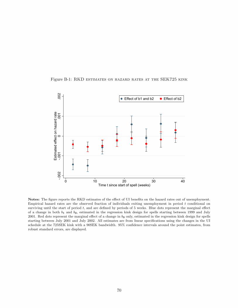
Figure B-1: RKD estimates on hazard rates at the SEK725 kink
-.002
-.001
0.0
01.0
02Es
timat
ed e
ffect
on
haza
rd ra
te
0 10 20 30 40Time t since start of spell (weeks)
Effect of b1 and b2 Effect of b2
Notes: The figure reports the RKD estimates of the effect of UI benefits on the hazard rates out of unemployment.Empirical hazard rates are the observed fraction of individuals exiting unemployment in period t conditional onsurviving until the start of period t, and are defined by periods of 5 weeks. Blue dots represent the marginal effectof a change in both b1 and b2, estimated in the regression kink design for spells starting between 1999 and July2001. Red dots represent the marginal effect of a change in b2 only, estimated in the regression kink design for spellsstarting between July 2001 and July 2002. All estimates are from linear specifications using the changes in the UIschedule at the 725SEK kink with a 90SEK bandwidth. 95% confidence intervals around the point estimates, fromrobust standard errors, are displayed.
70

B.2 RK design for D1 and D2
To assess the validity of the RK design for unemployment duration D1 spent on the first part of benefit profile and
unemployment duration D2 spent in the second part of the benefit profile, Figure B-2 below displays the raw data,
replicating for D1 and D2 what Figure 2 was doing for total unemployment duration D. The graphs provide graphical
evidence of a change in slope in the relationship between both D1 and D2 and previous daily wage in response to
the kink in UI benefits. The change in slope is larger for spells starting before July 2001, when both b1 and b2 are
capped at the 725SEK threshold. The magnitude of the change in slope decreases for spells starting between July
2001 and July 2002 when only b2 is capped at the 725SEK threshold. Formal estimates of the change in slope using
linear specifications of the form of equation (16) are displayed in Table 2. The red lines display predicted values of
the regressions in the linear case.
B.3 Year by year RKD estimates
Figure B-3 plots the year-by-year evolution of the estimates of the change in slope in the relationship between total
unemployment duration D and pre-unemployment daily wages from 1999 to 2007. The figure provides clear evidence
that our estimated responses are indeed due to the policy changes, and not due to time trends in the distribution of
durations around the kink.
71

Figure B-2: RK design at the SEK725 threshold for D1 and D2
1999-2000A. Outcome: D1 B. Outcome: D2
Kink in b1 and b2
1112
1314
15D
1: D
urat
ion
of u
nem
ploy
men
t cen
sore
d at
20
wee
ks
600 650 700 750 800 850Daily Wage (SEK)
Kink in b1 and b2
910
1112
1314
1516
17D
2: D
urat
ion
of u
nem
ploy
men
t afte
r 20
wee
ks600 650 700 750 800 850
Daily Wage (SEK)
2001C. Outcome: D1 D. Outcome: D2
Kink in b2 only
1112
1314
15D
1: D
urat
ion
of u
nem
ploy
men
t cen
sore
d at
20
wee
ks
600 650 700 750 800 850Daily Wage (SEK)
Kink in b2 only
910
1112
1314
1516
17D
2: D
urat
ion
of u
nem
ploy
men
t afte
r 20
wee
ks
600 650 700 750 800 850Daily Wage (SEK)
Notes: The Figure plots average unemployment duration D1 spent on the first part of benefit profile and averageunemployment duration D2 spent on the second part of the benefit profile, in bins of previous daily wage for the twoperiods of interest. Sample is restricted to unemployed individuals with no earnings who report being searching forfull-time employment. The graphs provide graphical evidence of a change in slope in the relationship between bothD1 and D2 and previous daily wage in response to the kink in UI benefits. The change in slope is larger for spellsstarting before July 2001, when both b1 and b2 are capped at the 725SEK threshold. The magnitude of the change inslope decreases for spells starting between July 2001 and July 2002 when only b2 is capped at the 725SEK threshold.Formal estimates of the change in slope using linear specifications of the form of equation (16) are displayed in Table2. The red lines display predicted values of the regressions in the linear case.
72

Figure B-3: RKD estimates on unemployment duration D at the SEK725 kink by yearof entry
Kinkin b1 & b2
Kinkin b2
No kink
-.075
-.05
-.025
0.0
25.0
5Es
timat
ed c
hang
e in
slo
pe
1999 2000 2001 2002 2003 2004 2005 2006Year of entry into unemployment
Notes: The figure reports the RKD estimates of the effect of UI benefits on total duration of unemployment by year
of entry into unemployment, at the 725SEK kink. Entry into unemployment in Year N is defined as starting a spell
between of July 1st of Year N and July 1st of Year N + 1. Spells starting before 2001 are therefore subject to a
kink in both b1 and b2. Spells starting in 2001 are subject to a kink in b2 only. Spells starting in 2002 and after
do not face any kink in the schedule and represent a placebo. All estimates are from linear specifications using the
changes in the UI schedule at the 725SEK kink with a 90SEK bandwidth. 95% confidence intervals around the point
estimates, from robust standard errors, are displayed. The figure provides clear evidence that estimated responses
in the RK design are indeed due to the policy changes, and not due to time trends in the distribution of durations
around the kink.
73

B.4 Additional robustness analysis of the RK design
This subsection presents various additional robustness checks of the RK design. We start by restating the two
fundamental identifying assumptions of the RK design, and then propose various tests to assess their potential
validity, by looking for clear violations of these assumptions.
We consider the general model:
Y = y(b1, b2, w, µ),
We are interested in identifying the marginal effect of benefits bk, k = 1, 2 on the duration outcome Y , αk = ∂Y∂bk
. bk
is a deterministic, continuous function of the wage w, kinked at w = wk. Identification of αk in the RK design relies
on two assumptions:
Assumption 1: the direct marginal effect of the assignment variable w on Y is assumed to be smooth around the
kink point wk. This means that ∂y(b1,b2,w,µ)∂w
is assumed to be continuous in the neighborhood of the kink point.
Assumption 2: the distribution of unobserved heterogeneity µ is assumed to be evolving smoothly around the kink
point. This means that the conditional density (fw|µ(·)) and its partial derivative with respect to w, (∂fw|µ(·)/∂w)
are assumed to be continuous in the neighbourhood of the kink point.
These identifying assumptions are, by definition, untestable. Yet, we can use the various “experiment arms” of
our quasi-experimental setting as well as sensitivity analysis to try to detect clear violations of these assumptions
and to provide some sense of the potential robustness of these identifying assumptions and the validity of our RK
design.
Testing for clear violations of Assumption 2: manipulation The most obvious violation of the assumption
of smooth distribution of heterogeneity at the kink arises if individuals are able to locate their daily wage strategically
around the kink point. A few tests can help assess the robustness of this assumption.
First, Figure B-4 plots the density of the daily wage and shows graphically the smoothness of the distribution of
the assignment variable at the kink point in the UI schedules. The graph shows the probability density function of
the daily wage around the 725SEK threshold and displays two formal tests. The first is a standard McCrary test of
the discontinuity of the pdf of the assignment variable. We report the difference in height of the pdf at the threshold.
The second is a test for the continuity of the first derivative of the p.d.f. We report the coefficient estimate of the
change in slope of the pdf in a regression of the number of individuals in each bin on polynomials of the assignment
variable interacted with a dummy for being above the threshold. Both tests suggest smoothness of the assignment
variable around the threshold
The continuity in the pdf of the assignment variable indicates that there is no bunching at the kink point. Such
bunching would have constituted proof of the ability of individuals to manipulate their location on the UI schedule,
which would have been a clear violation of Assumption 2. Absence of bunching at the kink is not a sufficient condition
to rule out that individuals respond to the kinked schedule in their earnings decision, which would question the validity
of Assumption 2. The absence of bunching could be driven by optimization frictions which attenuate the ability to
bunch at the kink, or by the fact that the compensated elasticity of daily wage with respect to marginal tax rates
is small. Even if the compensated elasticity of the daily wage is small, income effects could still be large, and would
affect earnings decisions as we move further away from the kink. This would then be picked up by variations in the
slope of the pdf at the kink. The fact that we do not detect any change in the first derivative of the pdf of daily wage
at the kink point, as reported in Figure B-4, is reassuring.
Interestingly, because the kinks in the schedule of b1 and b2 are removed in July 2001 and July 2002, we can
actually directly estimate whether the distribution of daily wages reacts to the removal of the kink and therefore
get a direct test of whether the pdf of the assignment variable is affected by the presence of the kink. In Table B-1
below, we report the results of a difference-in-difference model where we look at the evolution of log wages above and
below the kink, before July 2001 (when both kinks were in place) and after July 2001 (when one kink is removed).
74

The wages of individuals who had optimally chosen their daily wages at or above the kink, will be affected by the
removal of the kink. To the contrary, individuals who had optimally chosen daily wages below the kink should not be
affected by the removal of the kink. If individuals’ daily wages respond to the kinked UI schedule, we therefore expect
a differential change in the average log wages above the kink after July 2001 relative to log wages below the kink.
Estimates, reported in Table B-1 indicate that the removal of the kinks did not significantly affect the distribution
of daily wages above and below the kink. There is no differential change in the daily wage below and above the kink
after July 2001. This in turn suggests that the presence of kinks in the UI schedule does not significantly affect the
distribution of daily wages around the kink.
Testing for clear violations of Assumption 2: observable heterogeneity To further investigate the evolution
of the distribution of heterogeneity at the kink, the panels in Figure B-5 show how the mean values of different
covariates (age, fraction of men, highly educated and foreigners) evolve with the daily wage around the kink. We
do not find any non-linearity around the kink. This is also reassuring, as non-smoothness in the distribution of
observable heterogeneity would have cast doubt on the validity of the assumption of smoothness in the distribution
of unobservable heterogeneity around the kink.
Testing for underlying non-linearities: Bandwidth size The panels in Figure B-6 report our RKD estimates
for different bandwidth sizes. For all periods we consider, the estimates remain stable for bandwidths above h =
60SEK.
Testing for underlying non-linearities: Permutation tests Ganong and Jaeger [2014] suggest that it can be
helpful to assess whether the true coefficient estimate is larger than those at “placebo” kinks placed away from the
true kink. The idea behind their permutation test is that, if the counter-factual relationship between the assignment
variable and the outcome (i.e., in the absence of the kink in the budget set) is non-linear, then the curvature in this
relationship will result in many of the placebo estimates being large and statistically significant. In Table B-2, we
report 95% confidence interval based on this permutation procedure and compare them to bootstrapped standard
errors and robust standard errors.
Testing for underlying non-linearities: Non-parametric detection of kink point Figure B-10 shows the
R-squared when we run the RKD regression in (16) for “placebo” kinks placed in 10SEK increments from the true
location of the threshold. This procedure, proposed in Landais [2015], and inspired from the time series literature
on detection of trend breaks, enables to non-parametrically detect where a true kink is most likely to be located in
the data, by looking at the placebo kink where the R-squared is maximized. The figure shows that the R-squared is
maximized at the location of the actual kink point, again supporting the evidence that there is in fact a change in
slope that occurs at the actual kink point. In both panels A and B, the preferred location of the kink is extremely
close to the true kink and the relationship between the placebo kink location and R-squared of the model exhibits
a clear concave shape. In panel C, reassuringly, when there is no true kink at 725SEK, this relationship is perfectly
flat.
Polynomial order Table B-3 shows estimates of the change in slope at the kink for linear, quadratic and cubic
specifications, assessing the model fit for these different specifications.
For the 1999-2000 period, the estimates are very similar across polynomial orders. For the 2001 period, estimates
vary across polynomial orders, and estimates from the quadratic model are larger in magnitude than estimates using a
linear specification. Yet, model fit analysis suggests that linear estimates should be preferred. The linear specification
is having similar root mean squared errors (RMSE) and minimizes the Aikake information criterion (AIC). Note also
that, although larger, the point estimates on the quadratic specification are very imprecisely estimated, so that we
cannot actually reject that they are equal to the estimates from the linear model.
We also plot below in Figure B-8 the prediction from the linear and quadratic specifications on top of the raw
data to see how these models fit the data. For the period 1999-2000, panel A shows that both the quadratic and the
75

linear model fit the data equally well and deliver extremely similar results for the change in slope at the kink. For
the period 2001, the quadratic model delivers a larger change in slope at the kink compared to the linear fit. But
this is driven by a higher curvature so that the linear model overall does deliver a better fit of the data, as indicated
by the root squared mean error and the AIC reported on the graph.
Right-censoring When the schedule of benefits changes, individuals with ongoing spells are transferred to the
new schedule. To control for this, two solutions can be envisaged. First, one may get rid of observations who have
an ongoing spell at the moment the schedule changes. An alternative solution is to treat the duration of these
observations as censored at the moment when these individuals transfer the new schedule. One can then estimate a
Tobit model on the right-censored data. In Figure B-9 below, we report the estimates for the estimated change in
slope in D1 and D2 for censored and uncensored models, as a function of the RKD bandwidth. The Figure shows that
censored and uncensored models deliver identical results, and that the point estimates of the two models are never
statistically significantly different. The uncensored model proves a little less precise though, as we end up throwing
away some observations. As a consequence, we have decided to focus on the estimates from these censored models
for our baseline results.
76

Figure B-4: Robustness of the RK design: p.d.f of daily wage
McCrary testsDiscontinuity: 994.6 (596.5)
1st deriv. discontinuity: -31.1 (22.7)
015
000
3000
045
000
Num
ber o
f Obs
erva
tions
600 650 700 750 800 850Daily Wage (SEK)
Notes: The figure tests graphically the smoothness of the distribution of the assignment variable at the kink pointin the UI schedules to assess the validity of the local random assignment assumption underlying the RK design. ThePanel shows the probability density function of the daily wage around the 725SEK threshold. We also display twoformal tests of the identifying assumptions of the RKD. The first is a standard McCrary test of the discontinuity ofthe p.d.f of the assignment variable. We report the difference in height of the p.d.f at the threshold. The second is atest for the continuity of the first derivative of the p.d.f. We report the coefficient estimate of the change in slope ofthe p.d.f in a regression of the number of individuals in each bin on polynomials of the assignment variable interactedwith a dummy for being above the threshold. Both tests suggest smoothness of the assignment variable around thethreshold, in support of the identifying assumptions of the RK design.
77
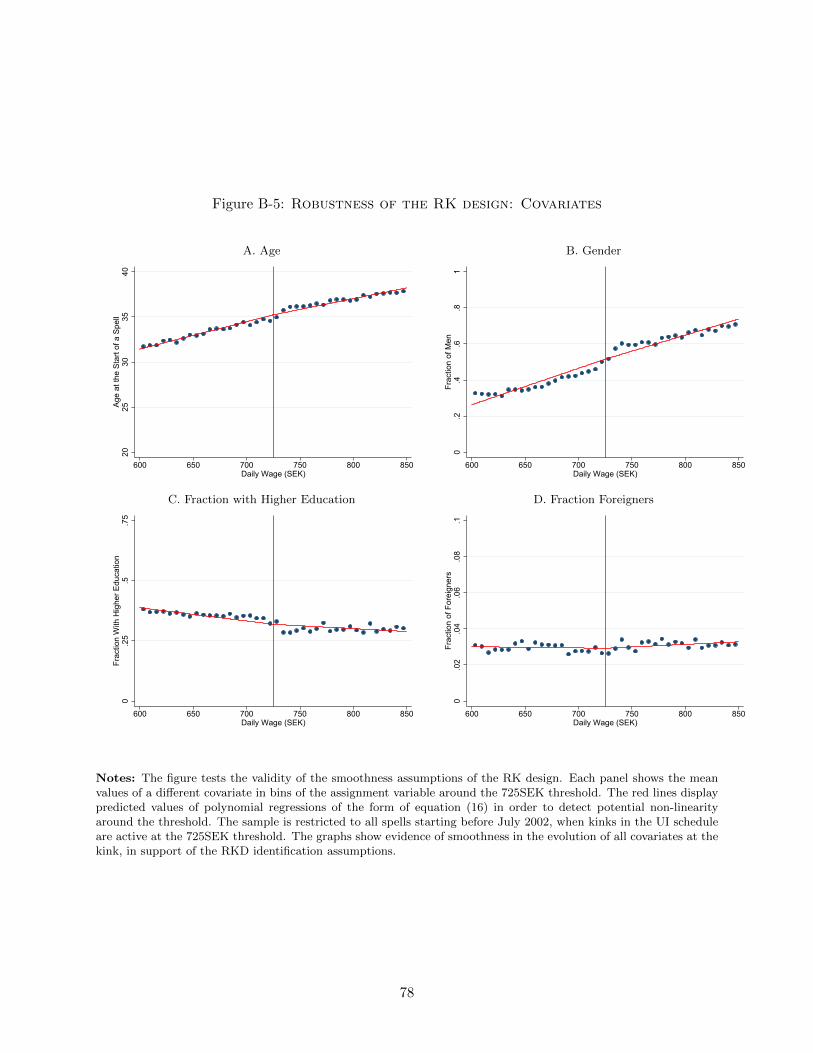
Figure B-5: Robustness of the RK design: Covariates
A. Age B. Gender
2025
3035
40Ag
e at
the
Star
t of a
Spe
ll
600 650 700 750 800 850Daily Wage (SEK)
0.2
.4.6
.81
Frac
tion
of M
en
600 650 700 750 800 850Daily Wage (SEK)
C. Fraction with Higher Education D. Fraction Foreigners
0.2
5.5
.75
Frac
tion
With
Hig
her E
duca
tion
600 650 700 750 800 850Daily Wage (SEK)
0.0
2.0
4.0
6.0
8.1
Frac
tion
of F
orei
gner
s
600 650 700 750 800 850Daily Wage (SEK)
Notes: The figure tests the validity of the smoothness assumptions of the RK design. Each panel shows the meanvalues of a different covariate in bins of the assignment variable around the 725SEK threshold. The red lines displaypredicted values of polynomial regressions of the form of equation (16) in order to detect potential non-linearityaround the threshold. The sample is restricted to all spells starting before July 2002, when kinks in the UI scheduleare active at the 725SEK threshold. The graphs show evidence of smoothness in the evolution of all covariates at thekink, in support of the RKD identification assumptions.
78

Figure B-6: RKD estimates as a function of bandwidth size
A. 1999 - 2000
-.1-.0
8-.0
6-.0
4-.0
20
.02
Estim
ated
Cha
nge
in S
lope
in D
25 50 75 100 125Bandwidth (Daily Wage (SEK)
B. 2001
-.1-.0
8-.0
6-.0
4-.0
20
.02
Estim
ated
Cha
nge
in S
lope
in D
25 50 75 100 125Bandwidth (Daily Wage (SEK)
79

Figure B-7: RKD estimates as a function of bandwidth size (continued)
A. 2002-2005
-.1-.0
50
.05
.1Es
timat
ed C
hang
e in
Slo
pe in
D
25 50 75 100 125Bandwidth (Daily Wage (SEK)
Notes: The figure reports estimates of the change in slope with 95% robust confidence interval in the relationshipbetween unemployment duration and daily wage at the 725SEK threshold using linear regressions of the form ofequation (16) as a function of bandwidth size h. These estimates are reported for three periods of interest: 1999-2000(i.e., spells starting before July 2001), 2001 (i.e., spells starting after July 2001 and before July 2002) and 2002-(i.e., spells starting after July 2002). Unemployment duration is defined as the number of weeks between registrationat the PES and exiting the PES or finding any employment (part-time or full-time employment, entering a PESprogram with subsidized work or training, etc.). Unemployment duration is capped at two years. Sample is restrictedto unemployed individuals with no earnings who report being searching for full-time employment.
80

Figure B-8: Unemployment duration as a function of daily wage around the 725SEKkink, and linear and quadratic model fits
A. 1999-2000
Linear modelRMSE=28.29AIC=1785650
Quadratic modelRMSE=28.29AIC=1785650
1520
2530
35D
urat
ion
of u
nem
ploy
men
t spe
ll
635 685 735 785 835Daily Wage (SEK)
B. 2001
Linear modelRMSE=27.612AIC=620999
Quadratic modelRMSE=27.612AIC=621001
1520
2530
35D
urat
ion
of u
nem
ploy
men
t spe
ll
635 685 735 785 835Daily Wage (SEK)
Notes: The figure plots average unemployment duration in bins of previous daily wage for spells starting before July2001 (panel A) and for spells starting between July 2001 and July 2002 (panel B). On top of the raw data, the figurealso displays predictions from linear and quadratic regressions of the form of equation (16) with a bandwidth sizeh = 90SEK. To further assess model fit, we report for each specification the root mean squared error (RMSE) as wellas the Aikake information criterion (AIC).
81
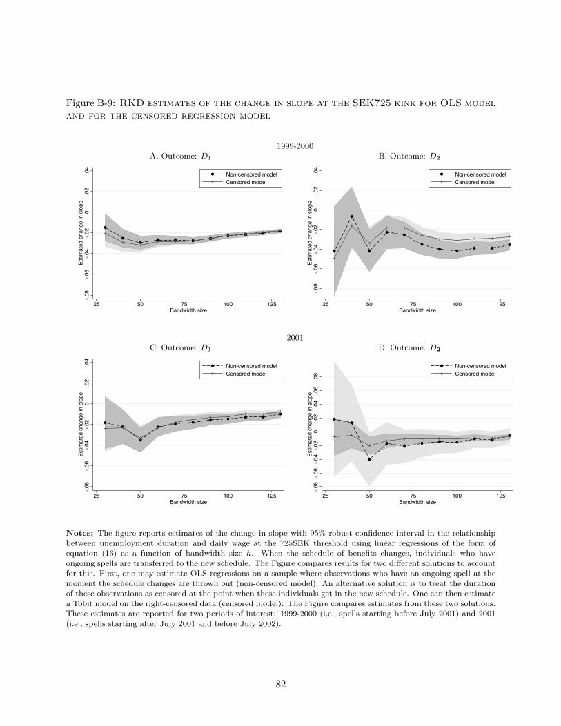
Figure B-9: RKD estimates of the change in slope at the SEK725 kink for OLS modeland for the censored regression model
1999-2000A. Outcome: D1 B. Outcome: D2
-.08
-.06
-.04
-.02
0.0
2.0
4Es
timat
ed c
hang
e in
slo
pe
25 50 75 100 125Bandwidth size
Non-censored modelCensored model
-.08
-.06
-.04
-.02
0.0
2.0
4Es
timat
ed c
hang
e in
slo
pe25 50 75 100 125
Bandwidth size
Non-censored modelCensored model
2001C. Outcome: D1 D. Outcome: D2
-.08
-.06
-.04
-.02
0.0
2.0
4Es
timat
ed c
hang
e in
slo
pe
25 50 75 100 125Bandwidth size
Non-censored modelCensored model
-.08
-.06
-.04
-.02
0.0
2.0
4.0
6.0
8Es
timat
ed c
hang
e in
slo
pe
25 50 75 100 125Bandwidth size
Non-censored modelCensored model
Notes: The figure reports estimates of the change in slope with 95% robust confidence interval in the relationshipbetween unemployment duration and daily wage at the 725SEK threshold using linear regressions of the form ofequation (16) as a function of bandwidth size h. When the schedule of benefits changes, individuals who haveongoing spells are transferred to the new schedule. The Figure compares results for two different solutions to accountfor this. First, one may estimate OLS regressions on a sample where observations who have an ongoing spell at themoment the schedule changes are thrown out (non-censored model). An alternative solution is to treat the durationof these observations as censored at the point when these individuals get in the new schedule. One can then estimatea Tobit model on the right-censored data (censored model). The Figure compares estimates from these two solutions.These estimates are reported for two periods of interest: 1999-2000 (i.e., spells starting before July 2001) and 2001(i.e., spells starting after July 2001 and before July 2002).
82

Figure B-10: Non-parametric detection of kink location
A. 1999 - 2000
.000
25.0
005
.000
75.0
01.0
0125
.001
5R
-squ
ared
of p
olyn
omia
l mod
el
600 650 700 750 800 850Location of placebo kink (daily wage SEK)
B. 2001
.000
25.0
005
.000
75.0
01.0
0125
.001
5R
-squ
ared
of p
olyn
omia
l mod
el
600 650 700 750 800 850Location of placebo kink (daily wage SEK)
83

Figure B-11: Non-parametric detection of kink location (continued)
C. 2002-2005
.000
25.0
005
.000
75.0
01.0
0125
.001
5R
-squ
ared
of p
olyn
omia
l mod
el
600 650 700 750 800 850Location of placebo kink (daily wage SEK)
Notes: The figure reports the R-squared of polynomial regressions of the form of equation (16) for alternative(placebo) locations of the kink point wk for all observations with wages between 625SEK and 825SEK. The red lineindicates the location of the true kink in the schedule. The dashed red line indicates the preferred location of the kinknon-parametrically detected in the data, maximizing the R-squared of the model. These estimates are reported forthree periods of interest: 1999-2000 (i.e., spells starting before July 2001), 2001 (i.e., spells starting after July 2001and before July 2002) and 2002- (i.e., spells starting after July 2002). In both panels A and B, the preferred locationof the kink is extremely close to the true kink and the relationship between the placebo kink location and R-squaredof the model exhibits a clear concave shape. In panel C, when there is no true kink at 725SEK, this relationship isperfectly flat.
84

Table B-1: Evolution of daily wages below and above the 725SEK point, before andafter kinks in the UI schedule are removed
(1) (2) (3)Dependent variable: log of daily wage
1[w > w] 0.120∗∗∗ 0.119∗∗∗ 0.119∗∗∗
(0.000146) (0.000146) (0.000147)
1[Spell > July2001] 0.00402∗∗∗ 0.00438∗∗∗ 0.00465∗∗∗
(0.000164) (0.000164) (0.000165)
1[Spell > July2001]× 1[w > w] 0.000305 0.000393 0.000519∗
(0.000222) (0.000222) (0.000222)
Age F-E × ×Education F-E ×Gender F-E ×Industry F-E ×
N 424309 424309 424309
Notes: Standard errors in parentheses.The Table tests for changes in the distribution of daily wages above and below the kink, as kinks in the schedule ofb1 and b2 are removed in July 2001 and July 2002. The table reports the results of a difference-in-difference modelof the form:
logw = β0 + β11[w > w] + β21[Spell > July2001] + β31[Spell > July2001]× 1[w > w] + η
The wages of individuals who had optimally chosen their daily wages at or above the kink, will be affected by the
removal of the kink. To the contrary, individuals who had optimally chosen daily wages below the kink should not
be affected by the removal of the kink. If individuals’ daily wages respond to the kinked UI schedule, we therefore
expect a differential change in the average log wages above the kink after July 2001 relative to log wages below the
kink, captured by β3. Estimates indicate that the removal of the kinks did not significantly affect the shape of the
distribution of daily wages above and below the kink.
85

Table B-2: RKD estimates at the 725SEK threshold: Inference
(1) (2) (3)Unemployment Duration D1 Duration D2
Duration D (< 20 weeks) (≥ 20 weeks)
I. 1999-2000: Kink in b1 and b2
Linear - δk -.0569 -.0246 -.0299Robust s.e. (.0047) (.0013) (.0036)Bootstrapped s.e. (.0050) (.0012) (.0039)95% CI - permutation test [-.0595 ; -.0566] [-.0319 ; -.0189] [-.0402 ; -.019]
II. 2001: Kink in b2 only
Linear - δk -.0255 -.0115 -.0105Robust s.e. (.005) (.0021) (.0028)Bootstrapped s.e. (.0049) (.0020) (.0030)95% CI - permutation test [-.0325 ; -.0190] [-.0127 ; -.0103] [-.0115 ; -.0091]
III. 2002-. : Placebo
Linear -δk .0045 -.0016 .006Bootstrapped s.e. (.0048) (.0011) (.0041)Robust s.e. (.0055) (.0011) (.0049)95% CI - permutation test [.0017 ; .0075] [-.0021 ; -.0011] [.0053 ; .0071]
Notes: The table reports estimates of the change in slope δk, at the 725SEK threshold, in the relationship betweendaily wage and the total duration of unemployment D (col. (1)), the time D1 spent on the first part of the SwedishUI profile (col. (2)) and the time D2 spent on the second part of the Swedish UI profile (col. (3)). D1 =
∑t<20wks St
corresponds to duration censored at 20 weeks of unemployment. D2 =∑t≥20wks St corresponds to unconditional
duration spent unemployed after 20 weeks of unemployment (i.e., not conditional on having survived up to 20 weeks).Estimates are obtained from linear regressions of the form of equation (16) with a bandwidth size h = 90SEK. Theseestimates are reported for three periods of interest. Panel I reports estimates for spells starting before July 2001.Panel II reports estimates for spells starting after July 2001 and before July 2002. Panel III reports estimates forspells starting after July 2002. Unemployment duration is capped at two years. We report for each estimate δkthe White robust standard errors, the bootstrapped standard errors using 50 replications, as well as 95% confidenceintervals using the permutation test method of Ganong and Jaeger [2014].

Table B-3: RKD estimates at the 725SEK threshold: Sensitivity to polynomial order
(1) (2) (3)Unemployment Duration D1 Duration D2
Duration D (< 20 weeks) (≥ 20 weeks)
I. 1999-2000: Kink in b1 and b2Linear - δk -.0569 -.0246 -.0299
(.0047) (.0013) (.0036)RMSE 28.285 7.049 23.972AIC 1785650.8 1264546 1723601.1
Quadratic - δk -.0474 -.0344 -.0183(.0185) (.0049) (.0143)
RMSE 28.285 7.048 23.971AIC 1785650.5 1264518.9 1723588.4
Cubic - δk -.0527 -.0291 -.0221(.0455) (.0122) (.0351)
MSE 28.284 7.046 23.971AIC 1785644.8 1264394.7 1723590
II. 2001: Kink in b2 onlyLinear - δk -.0255 -.0115 -.0105
(.0050) (.0021) (.0028)RMSE 27.612 6.863 23.512AIC 620999.2 438509.8 599929.6
Quadratic -δk -.0579 -.0299 -.0151(.0196) (.0098) (.011)
MSE 27.612 6.863 23.512AIC 621001.3 438509.9 599932.5
Cubic - δk -.0192 -.0268 .0068(.0485) (.0201) (.0274)
MSE 27.612 6.863 23.512AIC 621003.5 438508.6 599934.5
Notes: The table reports estimates of the change in slope δk, at the 725SEK threshold, in the relationship betweendaily wage and the total duration of unemployment D (col. (1)), the time D1 spent on the first part of the SwedishUI profile (col. (2)) and the time D2 spent on the second part of the Swedish UI profile (col. (3)). Estimates areobtained from polynomial regressions of the form of equation (16) with a bandwidth size h = 90SEK. Estimatesare reported for three different polynomial orders: the linear specification, the quadratic specification and the cubicspecification. For each polynomial order, we report model fit diagnostics: the root mean squared error (RMSE) aswell as the Aikake information criterion (AIC). Panel I reports estimates for spells starting before July 2001. PanelII reports estimates for spells starting after July 2001 and before July 2002. White robust standard errors are inparentheses.

B.5 Exploiting Other Kinks to Assess the Robustness of MH1 ≥MH2
The Swedish system offers during the period 1999 to 2007 various sources of variations that can be used to identify
MH1 andMH2. There are three simple reasons why the baseline estimates focus only on the kink at 725 SEK. First,
for expositional convenience: since all statistics of interest can be identified using the same RK design, this made
presenting the source of variation and the results particularly convenient. Second, for internal validity: comparing
estimates at the same kink ensures that we are comparing behavioral responses for comparable individuals over time.
And finally, for precision: there is more density around the 725SEK kink, which enables a higher degree of statistical
precision for the RK estimates
In this section, we investigate the robustness of our results to the use of other sources of variations. Indeed, one
may be worried that comparing individuals at the same kink over time may be problematic if behavioral elasticities
are prone to varying over time (due to business cycle variations for instance). In this sense, there is a trade-off
between comparing individuals at the same kink over time and comparing different individuals but in the same time
period. In the first case, one may worry that time affects behavioral elasticities, while in the second case, one may
worry that individuals at different kinks are different as they have different pre-unemployment incomes to start with.
In what follows, we review the different kinks and the sources of identification they provide, present our strategy
and estimates for each kink, and summarize the conclusions that we can draw from this evidence on the relative
magnitude of MH1 vs MH2. The bottom-line is that our estimates are very robust to using these alternative sources
of identification and in particular the larger magnitude of MH1 relative to MH2 is a very robust finding, irrespective
of the source of identification used.
B.5.1 850 SEK kink
In July 2001, the cap in b1, the UI benefits received during the first 20 weeks of unemployment, was increased to
680SEK, which created a kink in the relationship between b1 and the daily wage at a wage level of 850SEK. This
gives us the possibility to identify in the RK design the effect of b1 on duration outcomes. In July 2002, the cap in
b2, the UI benefits received after the first 20 weeks of unemployment, was increased to 680SEK, which created a kink
in the relationship between b2 and the daily wage at a wage level of 850SEK.
Figure B-11 reports the evolution of the RKD estimates of the change in slope in the relationship between
unemployment duration and daily wage at the 850 SEK kink, by year of entry into unemployment. Spells starting
before 2001 are subject to a linear schedule with no kink in either b1 nor b2 and represent the placebo. Spells starting
in 2001 are subject to a kink in b1 only. Spells starting in 2002 and after are subject to a kink in b2 only. The graph
provides clear evidence of a break in the relative slopes of the relationship between duration and wage on both sides
of the kink after the introduction of the kink in b1 in 2001. It also provides evidence of a slight decrease in the change
in slope as the kink in b1 is replaced by a kink in b2 after 2002.
Based on this evidence, we implement a DD-RKD in order to get estimates of the elasticities of duration with
respect to b1 and with respect to b2 at the 850SEK kink. Our DD-RKD specification is the following:
E[Y |w,P ] = β0 + β1(w − w) + δ0(w − w) · 1[w ≥ w]
+ 1[P = 1] ·(β2 + β3(w − w) + δ1(w − w) · 1[w ≥ w]
)+ 1[P = 2] ·
(β4 + β5(w − w) + δ2(w − w) · 1[w ≥ w]
).
(26)
where P denotes the time period in which the unemployment spell started. P = 0 for spells starting before July
2001, P = 1 for spells starting between July 2001 and July 2002 and P = 2 for spells starting after July 2002.
From this specification, we compute the implied benefit elasticities of unemployment duration. The elasticity of
duration with respect to b1, estimated at the 850SEK kink, is εD,b1 = δ1 · 850Dcap
, where δ1 is the estimated marginal
slope change for spells starting in period P = 1, and Dcap is the observed average duration at the kink for spells
starting in period P = 1. We find εD,b1 = 1.92 (.31). The elasticity of duration with respect to b2, estimated at the
88

850SEK kink, is εD,b2 = δ2 · 850Dcap
, where δ2 is the estimated marginal slope change for spells starting in period P = 2,
and Dcap is the observed average duration at the kink for spells starting in period P = 2. We find εD,b2 = 1.50 (.24).
B.5.2 912.5 SEK kink
In July 2002, the cap for b1, benefits received during the first 20 weeks of unemployment, was increased to 730SEK,
which created a kink in the schedule of benefits at a daily wage level of 912.5SEK. This gives us the possibility to
identify the effect of b1 on duration outcomes, using a RK design at the 912.5SEK kink.
As done previously at the 725SEK and 850SEK kink, Figure B-12 reports the evolution of the RKD estimates
of the change in slope in the relationship between unemployment duration and daily wage at the 912.5SEK kink, by
year of entry into unemployment. Spells starting before 2002 are subject to a linear schedule with no kink in either
b1 nor b2 and represent the placebo. Spells starting in 2002 and after are subject to a kink in b1 only. The graph
provides clear evidence of a break in the relative slopes of the relationship between duration and wage on both sides
of the kink after the introduction of the kink in b1 in 2002. However, estimates are much less precise than for the
other two kinks, as there is much less density around the 912.5SEK kink.
Based on this evidence, we also implement a DD-RKD in order to get estimates of the elasticities of duration
with respect to b1 at the 912.5SEK kink. Our DD-RKD specification is the following:
E[Y |w,P ] = β0 + β1(w − w) + δ0(w − w) · 1[w ≥ w]
+ 1[P = 2] ·(β4 + β5(w − w) + δ2(w − w) · 1[w ≥ w]
). (27)
where P denotes the time period in which the unemployment spell started, with P = 2 for spells starting after July
2002.
From this specification, we compute the implied benefit elasticities of unemployment duration. The elasticity of
duration with respect to b1, estimated at the 912SEK kink is εD,b1 = δ2 · 912.5Dcap
, where δ1 is the estimated marginal
slope change for spells starting in period P = 2, and Dcap is the observed average duration at the kink for spells
starting in period P = 2. We find εD,b1 = 2.15 (.70).
B.5.3 Combining estimates to identify the relative magnitude of MH1 vs MH2
Based on these sources of variations, we now have four different potential estimates of the relative moral hazard costs
of b1 vs b2, summarized in Table B-4 below
The first strategy consists in comparing estimates at the same “kink” over time. This approach, as mentioned
earlier, has the advantage of comparing similar individuals over time at the same level of income. One drawback
may be that behavioral elasticities are time varying due to business cycle fluctuations for instance. Two kinks, the
725SEK kink and the 850SEK kink, allow us to implement this first strategy, giving us two different estimates of the
moral hazard costs ratio, displayed in panel A and panel B of Table B-4. Results using estimates at the 725SEK
kink represent our baseline strategy, displayed in panel A, and compare estimates from 1999-2000 versus 2001, taking
advantage of the fact that at the 725SEK kink, we can identify εD,b in 1999-2000 and εD,b2 in 2001. From this
baseline strategy, we find a ratio MH1/MH2 = 1.264, as shown in panel A of Table B-4
Results using estimates at the 850SEK kink over time are displayed in panel B, and compare estimates from 2001
versus 2002-2007, taking advantage of the fact that at the 850SEK kink, we can identify εD,b1 in 2001 and εD,b2 in
2002-2007. From this strategy, we find a ratio MH1/MH2 = 1.155, as shown in panel B of Table B-4. Estimates of
the moral hazard cost ratio from panel A and B are very similar. This confirm that the relative magnitude of the
moral hazard costs is very robust across kinks, alleviating the concern that the moral hazard cost ratio is extremely
sensitive to the location of the income distribution at which it is estimated.
The second strategy consists in comparing estimates at different “kinks” within the same time period. This
second approach has the advantage of comparing individuals within the same time period, therefore controlling for
89

the fact that behavioral elasticities may be time varying due to business cycle fluctuations for instance. A potential
drawback of this approach is that individuals at different kinks may differ in their responsiveness to the policy.
Two time periods, 2001 and 2002-2007 allow us to implement this second strategy, giving us two additional
estimates of the moral hazard costs ratio, displayed in panel C and panel D of Table B-4. For the 2001 period,
we have estimates of MH1 from the 850SEK kink and estimates of MH2 from the 725SEK kink. Combining these
estimates, we get a ratio MH1/MH2 = 2.695, as shown in panel C of Table B-4. For the 2002-2007 period, we
have estimates of MH1 from the 912.5SEK kink and estimates of MH2 from the 850SEK kink. Combining these
estimates, we get a ratio MH1/MH2 = 1.343 , as shown in panel C of Table B-4. Again, both estimates of the MH
cost ratio confirm that the moral hazard cost of b1 is larger than the moral hazard cost of b2 in our context.
Results from Table B-4 therefore all strongly suggest that our finding that MH1 > MH2 is robust to the sources
of variations used to estimate the effects of b1 and b2 on unemployment durations. We believe these results to be
an important piece of additional evidence on the validity and robustness of our findings on the relative magnitude of
moral hazard costs over the unemployment spell.
B.5.4 Inference on estimates of the relative magnitude of MH1 vs MH2
To provide inference on our estimates of the relative magnitude of MH1 vs MH2, we adopt a permutation-test
approach. Since our estimation approach relies on a comparison of two kinks, either over time, or within period, we
replicate this comparison for placebo kinks drawn at random in the distribution of daily wage in regions where the
UI benefit schedule does not exhibit any kink.
For panel A, we draw 250 kinks at random. For each kink, we estimate the change in slope in 1999-2000 and
2001 and from this obtain a distribution of 250 placebo estimates of the moral hazard MH1 and MH2. In Figure
B-13 panel A, we draw the distribution of the placebo estimates of the difference MH1 −MH2 obtained from this
procedure. As can be seen, this distribution is centered around 0, and our true estimate obtained from the 725SEK
kink lies far in the upper tail of this distribution of placebo estimates. This procedure gives us a p-value of 5.98%
for our estimate of the relative magnitude of MH1 −MH2. In other words, this procedure is providing compelling
evidence that our estimates of the relative moral hazard costs are not picking up some random variation in the slope
of the relationship between durations and daily wage over time.
Similarly, for panel B, we draw again 250 kinks at random. For each kink, we estimate the change in slope in
2001 vs 2002-2007 and from this obtain a distribution of 250 placebo estimates of the moral hazard MH1 and MH2.
In Figure B-13 panel B., we draw the distribution of the placebo estimates of the difference MH1 −MH2 obtained
from this procedure. Again, this procedure confirms that our estimates of the relative moral hazard costs is not
picking up some random variation in the slope of the relationship between durations and daily wage over time. From
this distribution of placebo kinks, the p-value for our estimate in Table B-4 panel B is 0.00%.
Similarly, for panel C, we draw 250 kinks at random from which we can generate 31,000 (= 2502
2− 250) pairs
of RKD estimates for the period July 2001 to July 2002. For each pair of kink, we estimate the changes in slope in
2001 and from this obtain a distribution of 31,000 placebo estimates of the moral hazard MH1 and MH2. In Figure
B-13 panel C, we draw the distribution of the placebo estimates of the difference MH1 −MH2 obtained from this
procedure. Results again provide compelling evidence that our estimates of the relative moral hazard costs in panel
C of Table B-4 are not picking up some random variation in the slope of the relationship between durations and daily
wage across different kinks in the 2001 period. The p-value for our estimate in Table B-4 panel C that we obtain
from this permutation procedure is 0.00%.
Finally, for panel D, we draw 250 kinks at random from which we can generate 31,000 (= 2502
2− 250) pairs of
RKD estimates for the period 2002 to 2007. For each pair of kink, we estimate the changes in slope in 2002-2007 and
from this obtain a distribution of 31,000 placebo estimates of the moral hazard MH1 and MH2. In Figure B-13 panel
D., we draw the distribution of the placebo estimates of the difference MH1 −MH2 obtained from this procedure.
This gives us a p-value for our estimate in Table B-4 panel D of 2.63%.
90

Figure B-11: RKD estimates on unemployment duration D at the 850SEK kink by yearof entry
1R.LQN .LQNLQE .LQNLQE
(VWLP
DWHGFKDQJHLQVORSH
<HDURIHQWU\LQWRXQHPSOR\PHQW
Notes: The figure reports the RKD estimates of the effect of UI benefits on total duration of unemployment byyear of entry into unemployment, at the 850SEK kink. Entry into unemployment in Year N is defined as starting aspell between July 1st of Year N and July 1st of Year N + 1. Spells starting before 2001 are therefore subject to asmooth linear schedule with no kink in either b1 nor b2 and represent the placebo. Spells starting in 2001 are subjectto a kink in b1 only. Spells starting in 2002 and after are subject to a kink in b2 only. All estimates are from linearspecifications using the changes in the UI schedule at the 850SEK kink with a 90SEK bandwidth, and are relative toyear 2000, which is the baseline. 95% confidence interval around the point estimates, from robust standard errors,are displayed. The figure provides clear evidence that estimated responses in the RK design are indeed due to thepolicy changes, and not due to time trends in the distribution of durations around the kink.
91

Figure B-12: RKD estimates on unemployment duration D at the 912.5SEK kink byyear of entry
1R.LQN .LQNLQE
(VWLP
DWHGFKDQJHLQVORSH
<HDURIHQWU\LQWRXQHPSOR\PHQW
Notes: The figure reports the RKD estimates of the effect of UI benefits on total duration of unemployment by yearof entry into unemployment, at the 912.5SEK kink. Entry into unemployment in Year N is defined as starting a spellbetween of July 1st of Year N and July 1st of Year N + 1. Spells starting before 2002 are subject to a smooth linearschedule with no kink in either b1 nor b2 and represent the placebo. Spells starting in 2002 and after are subject toa kink in b1 only. All estimates are from linear specifications using the changes in the UI schedule at the 912.5SEKkink with a 60SEK bandwidth, and are relative to year 2001, which is the baseline. 95% confidence interval aroundthe point estimates, from robust standard errors, are displayed.
92
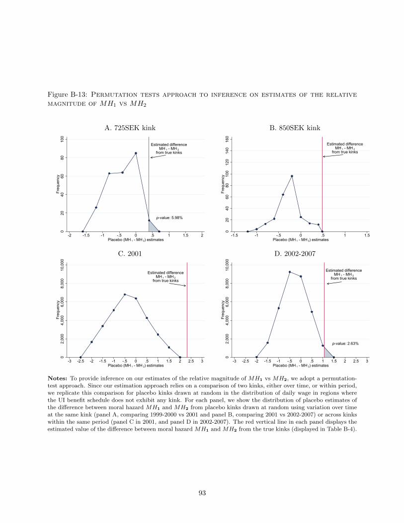
Figure B-13: Permutation tests approach to inference on estimates of the relativemagnitude of MH1 vs MH2
A. 725SEK kink B. 850SEK kink
Estimated differenceMH 1 - MH 2
from true kinks
p-value: 5.98%
020
4060
8010
0Fr
eque
ncy
-2 -1.5 -1 -.5 0 .5 1 1.5 2Placebo (MH 1 - MH 2) estimates
Estimated differenceMH 1 - MH 2
from true kinks
020
4060
8010
012
014
016
0Fr
eque
ncy
-1.5 -1 -.5 0 .5 1 1.5Placebo (MH 1 - MH 2) estimates
C. 2001 D. 2002-2007
Estimated differenceMH 1 - MH 2
from true kinks
02,
000
4,00
06,
000
8,00
010
,000
Freq
uenc
y
-3 -2.5 -2 -1.5 -1 -.5 0 .5 1 1.5 2 2.5 3Placebo (MH 1 - MH 2) estimates
Estimated differenceMH 1 - MH 2
from true kinks
p-value: 2.63%
02,
000
4,00
06,
000
8,00
010
,000
Freq
uenc
y
-3 -2.5 -2 -1.5 -1 -.5 0 .5 1 1.5 2 2.5 3Placebo (MH 1 - MH 2) estimates
Notes: To provide inference on our estimates of the relative magnitude of MH1 vs MH2, we adopt a permutation-test approach. Since our estimation approach relies on a comparison of two kinks, either over time, or within period,we replicate this comparison for placebo kinks drawn at random in the distribution of daily wage in regions wherethe UI benefit schedule does not exhibit any kink. For each panel, we show the distribution of placebo estimates ofthe difference between moral hazard MH1 and MH2 from placebo kinks drawn at random using variation over timeat the same kink (panel A, comparing 1999-2000 vs 2001 and panel B, comparing 2001 vs 2002-2007) or across kinkswithin the same period (panel C in 2001, and panel D in 2002-2007). The red vertical line in each panel displays theestimated value of the difference between moral hazard MH1 and MH2 from the true kinks (displayed in Table B-4).
93

Table B-4: Summary of Moral Hazard Cost Ratio Estimates
I. Using Same Kink, Over Time
A. 725 SEK - Kink B. 850 SEK - Kink
δb1 -0.036 -0.060(0.007) (0.009)
Variation used ’99-’00 vs 2001 kink 2001 kink
δb2 -.0255 -0.047(.0049) (0.007)
Variation used 2001 kink 2002-2007 kink
MH1MH2
1.264 1.155
p-value 5.98% 0.00%
II. Using Different Kinks Within Same Time Period
C. 2001 D. 2002-2007
δb1 -0.060 -0.062(0.009) (0.02)
Variation used 850SEK kink 912.5SEK kink
δb2 -0.023 -0.047(0.008) (0.007)
Variation used 725SEK kink 850SEK kink
MH1MH2
2.695 1.343
p-value 0.00% 2.63%
Notes: The Table reports all the different estimates of the moral hazard cost ratios that can be drawn from thesystematic exploitation of the kinks in the UI benefit schedule in Sweden over the period 1999 to 2007. Panel Ireports estimates from the strategy consisting in comparing estimates at the same “kink” over time. This approachhas the advantage of comparing similar individuals over time at the same level of income. Two kinks, the 725SEKkink and the 850SEK kink, allow us to implement this strategy, giving us two different estimates of the moral hazardcosts ratio, displayed in panel A and panel B. Panel II reports estimates from the strategy consisting in comparingestimates at different “kinks” in the daily wage distribution within the same time period. This second approach hasthe advantage of comparing individuals within the same time period, therefore controlling for the fact that behavioralelasticities might be time varying due to business cycle fluctuations for instance. Two time periods, 2001 and 2002-2007 allow us to implement this second strategy, giving us two additional estimates of the moral hazard costs ratio,displayed in panel C and panel D. For each estimate of the moral hazard cost ratio, we report the RKD estimateof the effect on duration D of the change in slope for variation in b1 (δb1) and the estimate of the change in slopefor variation in b2 (δb2), along with their standard errors in parenthesis. Below each RKD estimate δb1 and δb2 , wedisplay the source of variation used for identification. Below each estimate of the MH cost ratio, we display p-valuesfrom a permutation based test, using placebo kinks drawn at random in the distribution of daily wage in regionswhere the UI benefit schedule does not exhibit any kink. See text for details.
94

B.6 Comparison to Duration Response Estimates in the Literature
How do our duration response estimates compare to existing estimates of labor supply responses to UI benefits
available in the literature? To answer this question, we first need to be very precise about the source of variation of
benefits used for the estimates against which we want to benchmark our estimates. As our conceptual analysis makes
very clear, elasticity of duration w.r.t benefits paid early during the spell or w.r.t benefits paid later during the spell
are conceptually different, and will likely be very different empirically, especially in the presence of non-stationary
forces.
The elasticities εDk,bthat we report in Table 2 column (1) in the main text are unique, compared to estimates
in the literature, because they measure duration responses to a unique form of benefit variation. To understand this,
remember that the potential duration of benefits being infinite in the Swedish system during our period of analysis,
individuals can collect these benefits indefinitely. This means that the elasticity εDk,bthat we report measures the
response of duration to a change in benefits forever. We do not know of any other paper using similar source of
variation. The reported elasticities with respect to this unique source of variation appear quite large at first glance,
but it might not be that surprising, and it is hard to gauge these magnitudes using available benchmarks.
To appreciate the magnitude of our duration responses, it is therefore better to focus on elasticities that use
variations in benefits that are similar to the ones used in the previous literature. Our elasticity of time spent in the
first part of the profile D1 with respect to b1, the benefits that you receive in the first 20 weeks is, in this respect,
probably the best candidate. It can for instance be compared to estimates of the elasticity of paid unemployment
duration (unemployment duration up to exhaustion) with respect to a variation in UI “benefit level” in the US,
given individuals receive these benefits only in the first 26 weeks in the US. Put it differently, the elasticity of paid
unemployment duration with respect to a variation in UI “benefit level” in the US is conceptually equivalent to our
estimate of εD1,b1 , with the slight difference that b1 is given for 20 weeks in Sweden instead of 26 weeks in the US,
and D1 is the duration up to 20 weeks while the duration of paid unemployment is the duration up to 26 weeks in
the US.65 Our estimate εD1,b1 from the 725 SEK kink is .71 (.10). This estimate is in line with available estimates of
the elasticity of paid unemployment duration with respect to a variation in UI “benefit level” in the US. The classic
study is for instance Meyer [1990], who found an elasticity of .56.66 Landais [2015] indeed finds a slightly smaller
elasticity (around .4). Kroft and Notowidigdo [2016] find an elasticity of .63 (.33) at the average unemployment rate
in the US (p.20, based on estimates in Table 2 column 1) and conclude that such estimate “is broadly similar to the
previous literature (Moffitt 1985, Meyer 1990, Chetty 2008)”.
This evidence suggests that when benchmarked against conceptually similar elasticities, our duration responses
prove quite similar to moral hazard estimates available in the literature.
65Of course, even if they are conceptually similar, the two elasticities do not need to be the same. One obviousreason they may differ is that these elasticities are potentially endogenous to b2, and b2 = 0 in the US, while b2 = b1in Sweden.
66See Meyer [1990], Table VI, column (7). Coefficient estimates for log(b) in the proportional hazard models can beinterpreted as the elasticity of the hazard rate s with respect to the benefit level. However, under the assumption thatthe hazard rate is somewhat constant, these elasticities can be interpreted as elasticities of unemployment duration,since D ≈ 1/s so that εD ≈ −εs
95

FOR ONLINE PUBLICATION - Appendix C: Additional results
and robustness of consumption analysis
This Appendix presents the construction of our residual measure of consumption expenditures based on registry data.
It also presents additional results on consumption patterns over the unemployment spell and dynamic selection. It
finally compares our results to results obtained using household consumption surveys (HUT), for which we can also
explore patterns of consumption over the spell across different categories of expenditures.
C.1 Registry-based measures of consumption
We start by describing the construction of a registry-based consumption expenditure measure and we explain how it
can be used it to present complementary analysis of how consumption evolves during the unemployment spell.
The registry-based measure of consumption is based on exhaustive administrative information on income, trans-
fers and wealth in Sweden accounting for all income sources and changes in assets. The measure offers the advantage
of being computable for the universe of unemployed households from 1999 to 2007. The measure captures annual
expenditures between December of each year.
We start from the accounting identity that expenditures in year n are the sum of all income and transfers received
in period n, minus the change in assets between year n− 1 and year n,
expendituresn = incomen −∆assetsn.
As a result of the comprehensiveness of the longitudinal administrative dataset that we assembled including all
earnings, income, taxes, transfers and wealth, we have precise third-party reported information on all the compo-
nents needed to construct such residual measure of yearly expenditures for the universe of Swedish individuals and
households for years 1999 to 2007.
Our approach builds on previous attempts to measure consumption from registry-data (e.g. Browning and Leth-
Petersen [2003]) and in particular on Koijen et al. [2014] who constructed a similar measure in Sweden for years
2003 to 2007 using a smaller subset of individuals, and confirmed its consistency with HUT data. Our approach
extends these previous attempts and is closely related to Eika et al. [2017] in exploiting additional information on
asset portfolio choices and returns to reduce measurement error and excess dispersion of consumption measures based
solely on first-differencing asset stocks.
For interested readers, Kolsrud et al. [2017], (in preparation for a special issue of the Journal of Public Economics
dedicated to the use of new data sources for consumption analysis), offers all the details of the construction of our
residual measure of consumption. In particular, it provides information on all the registers, variables and programs
needed to construct a reliable registry-based measure of consumption from the Swedish administrative data, and
explains how to use flow transaction information on assets (real estate assets and financial assets) rather than first-
differences in asset stocks over time to reduce measurement error.
In practice, we compute consumption in year n as:
Cn = yn + Tn + Cbn + Cdn + Cvn + Chn ,
where:
• yn represents all earnings and is computed from the tax registers, which contain third-party reported earnings
for all employment contracts, including all fringe benefits and severance payments.67
• Tn accounts for all income taxes and transfers, including unemployment insurance, disability insurance, sick
pay, housing and parental benefits, etc.
67Note that self-employed, for whom earnings are in large part self-reported, are excluded from the analysis as theyare part of a different UI system.
96

• Cbn = ybn − ∆bn equals consumption out of bank holdings. It is equal to interests earned on these bank
holdings during year n, ybn, minus the change in the value of bank holdings between year n − 1 and year n,
∆bn = bn − bn−1.
• Cdn = −ydn + ∆dn is consumption out of debt, which includes student loans, credit card debt, mortgages, etc.,
and is third-party reported by financial institutions to the tax authority. It is equal to the change in the stock
of debt ∆dn, minus all interests paid on the existing stock of debt ydn.
• Cvn = yvn − ∆vn is consumption out of financial assets (other than liquid holdings in bank accounts). It is
equal to all income from financial assets yvn minus the change in the value of the portfolio of financial assets
∆vn. The return on financial assets yvn includes interests, dividends and any price change ∆pvn × qvn. Such
price change would be exactly offset by a change in the value of assets, included in ∆vn, unless the return is
realized by selling the asset. In practice, to separate the contribution of price changes from contribution of
asset rebalancing, we use detailed data collected by Statistics Sweden from banks and financial institutions
on all financial securities held by individuals, which contain information on quantities, ISIN numbers, and
transaction values and dates.
• Chn = yhn − ∆hn constitutes consumption out of real estate wealth. It is equal to all income derived from
holding real estate assets yhn minus the change in the value of real estates ∆hn. Detailed information on the
stock of real estate wealth, estimated at market value as of December 31 of each year, is available from the tax
authority. The return to holding real estate yhn includes rents, but also imputed rents for homeowners, as well
as price changes in the value of real estates. Such price change would again be exactly offset by a change in the
value of real estate assets, included in ∆hn, unless the return is realized by selling the asset. To separate the
contribution of price changes from contribution of real estate buying/selling, we use the housing transaction
register which collects information on all real estate transactions operated in Sweden.
All income, transfers and asset positions are reported to the tax administration (and observed in the data) at
the individual level.68 We have aggregated consumption measures at the household level using household identifiers
constructed by the Swedish National Statistical Office (Statistics Sweden).
C.2 Consumption patterns prior to the onset of a spell
To recover the drops in the first and second part of the profile from drops in annual consumption expenditures,
our baseline implementation in section 4.1 makes the assumption that cj = c0, ∀j < 0, or in other words, that the
consumption profile is flat prior to the start of an unemployment spell. To investigate how consumption profiles
evolve prior to the unemployment spell we report in Figure C-1 the annual log household consumption changes as a
function of time t since the onset of a spell, Ci,t − Ci,t−52 in 5 weeks bins, relative to the last 5 weeks prior to the
onset of a spell. We go as far back as 4 years prior to the onset of a spell, to detect longer anticipation effects. The
Figure shows two interesting patterns. First, the consumption patterns of households are extremely stable in the 4
years prior to displacement, suggesting no long term anticipation behaviors. Second, there does not seem to be any
sharp consumption changes immediately preceding displacement, suggesting no significant short term anticipation
behaviors. Overall, this evidence strongly supports the assumption that flow consumption profiles are flat prior to
the onset of an unemployment spell.
68It is possible that our measure misses some financial wealth held in foreign banks to the extent that these banksdo not comply with the requirement to transmit information on the financial wealth of their Swedish customers tothe Swedish tax authority. Yet, the fraction of foreign-held assets is low (about 3% of household assets according tothe Savings Barometer of Statistics Sweden), and likely to be held by much wealthier households than our sample ofunemployed.
97

Figure C-1: Change in log annual consumption as a function of time since onset ofan unemployment spell: pre-unemployment trends
-.4-.3
-.2-.1
0.1
Estim
ated
Ann
ual L
og C
onsu
mpt
ion
Cha
nge
-208 -182 -156 -130 -104 -78 -52 -26 0 26 52Event Time (Weeks)
Notes:The Figure investigates the validity of the assumption of a flat profile of consumption pre-unemployment. Wereport the annual log household consumption changes as a function of time t since the onset of a spell, ln Ci,t−ln Ci,t−52
in 5 weeks bins, relative to the last 5 weeks prior to the onset of a spell. Estimates provide compelling evidence thatconsumption profiles are flat prior to the onset of an unemployment spell.
98

C.3 Additional Results on Consumption Smoothing Means & Dynamic Selec-
tion
Assets and liquidity constraints In this subsection, we discuss the evidence of the role of assets and
liquidity constraints in consumption smoothing over the spell. First, we report in Appendix Figure C-2, and following
the same methodology as in Figure 6, the average annual consumption drops by time spent unemployed as of
December, breaking down the sample by the level of net wealth of the household at the start of the spell. The Figure
shows that households with higher net wealth experience a lower drop in consumption conditional on unemployment
duration. These households tend to have a smoother consumption profiles during unemployment, especially earlier
on in the spell.
Second we provide direct evidence that individuals do use their liquid assets to smooth consumption over the spell.
In Appendix Figure C-3 panel A, we estimate average change in liquid bank holdings compared to pre-unemployment
by time t spent unemployed as of December (when bank holding stock is observed in the registry data). Estimates of
the change in bank holdings B are scaled by the average annual consumption in the last year prior to unemployment,
so that all changes in bank holdings are expressed relative to pre-unemployment household consumption levels. The
Figure provides evidence that households use their liquid assets to smooth consumption over the unemployment spell,
by depleting their bank accounts or reducing their savings. This source of consumption smoothing remains small in
magnitude, as even after more than a year of unemployment, the change in bank holdings represent around 2% of
pre-unemployment consumption levels of the household.
In panel B of Appendix Figure C-3 we report similar estimates for all other assets. The Figure shows that the
change in total net assets other then bank holdings represent ≈2.5% of pre unemployment consumption after a year
in unemployment.
Finally, evidence from registry data also indicates that debt does not offer much help in smoothing consumption
over the unemployment spell, hinting at the presence of liquidity constraints. In Appendix Figure C-4, we provide
evidence of a reduction in the use of non mortgage-related credit over the unemployment spell among households with
no real estate and no mortgage debt. This Figure shows average change in debt compared to pre-unemployment by
time t spent unemployed as of December (when debt level is observed in the registry data). The sample is restricted to
individuals with no real estate wealth throughout the sample period. Because we cannot precisely separate mortgage
debt from other types of credit in the data, this sample restriction is a direct way to identify how non-mortgage
related debt evolves over the unemployment spell. The Figure provides evidence that households reduce their debt
level rather than increase it as they become unemployed. Instead of contributing positively to consumption smoothing,
debt contributes negatively to consumption over the unemployment spell. This suggests that as the duration of the
spell increases, access to credit becomes harder and consumption out of debt falls significantly.
Overall, this analysis confirms that households may have means to smooth consumption over short spells. But as
the duration of the spell increases, these means get quickly exhausted. Households in the second part of the profile
seem therefore closer to being hand-to-mouth.
Spousal Labor Supply Within a household, the labor supply of other members of the household may help
reduce the drop in household consumption over the spell. In Figure C-5 we investigate how labor supply of other
members of the household affects the drop in household consumption over the spell. Following the same methodology
as in Figure 6, we report the average change in total gross earnings and in total disposable income of all other
members of the household as a function of time spent unemployed, scaled by the annual household consumption level
prior to unemployment. Individual disposable income include all individual taxes and transfers, as well as individual
capital gains and losses.
Results show that within-household changes in the earnings and disposable income of all other members of the
household are small and almost always not significantly different from zero throughout the unemployment spell. This
suggests that in our context, the labor supply of other members of the household does not play a significant role in
smoothing household consumption even for long-term unemployed. This may be because the added-worker effect is
not playing a significant role in increasing household consumption in response to an unemployment shock, or because
99

its effect is mitigated by correlated earnings shocks across household members.
Dynamic Selection In practice, agents are heterogeneous and selection into longer unemployment spells
may affect consumption responses over the spell and the gradient of consumption smoothing gains. To assess the
potential magnitude of dynamic selection on consumption and risk preferences, we investigate in Table C-1 how various
observable characteristics that have been shown to correlate with consumption and risk preferences are distributed
across short term and long term unemployed.
To do so, we restrict the sample to all individuals about to become unemployed in the next quarter and estimate
a linear probability model where the outcome is an indicator variable for experiencing a future spell longer than 20
weeks. The default age category is 18 to 30 years old. Income refers to individual disposable income and results are
relative to the first quintile. Net wealth results are relative to individuals with zero or negative net wealth at the
start of the spell. We also investigate the effect of two portfolio characteristics, that, conditional on net wealth, are
traditionally correlated with risk preferences. First, we look at the fraction of total wealth invested in stocks, and
results are relative to the first two quartile of this distribution (50% of the sample have zero stocks prior to becoming
unemployed). Second, we look at leverage defined as total debt divided by gross assets, and results are relative to
the first quartile of leverage.
The patterns of selection are generally small in magnitude and often ambiguous in sign. Income levels and
net wealth levels have quantitatively small and non-monotonic effects on the probability to select into longer spells.
Compared to households with no or negative net wealth, households with some small wealth (<500kSEK) have a
slightly lower probability to be long term unemployed. But individuals with high net wealth have a slightly higher
probability to select into long spells. This result suggests that in our context, individuals with better means to smooth
consumption do not unambiguously select into longer spells, which corroborates the evidence of no clear patterns
of selection on consumption profiles displayed in subsection 4.1. Also portfolio characteristics (i.e., the fraction of
portfolio wealth invested in stocks, and leverage defined as total debt divided by gross assets), which have been
shown to be correlated with risk preferences, have small and non-monotonic impacts on the probability to experience
a long unemployment spell. In contrast, the probability of experiencing long unemployment spells (1[L > 20 wks])
is significantly and monotonically correlated with age. However, existing evidence from the literature suggests a
U-shape relationship between age and risk aversion (Cohen and Einav [2007]), so the dynamic selection on age has
an ambiguous effect on the evolution of risk preferences over the spell.
Overall, the observed dynamic selection patterns on consumption and risk preferences do not suggest that relative
consumption smoothing gains would be significantly different than our estimates based on the average drops in
consumption.69
69Yet, other methods exploiting comparative statics of effort choices as in Chetty [2008a], or Landais [2015], couldalso be developed to evaluate the evolution of consumption smoothing gains over the spell. These methods couldcircumvent the issue of having to make assumptions regarding dynamic selection on risk preferences.
100

Figure C-2: Estimated Drop in Annual Consumption Relative to Pre-Unemploymentas a Function of Time Spent Unemployed: Heterogeneity By Level of Wealth
A. Above Median Wealth Level Pre-Unemployment
Estimated Drop in Log Consumption (Flow)First 20 weeks: ∆c1 = -.029 (.015)After 20 weeks: ∆c2 = -.083 (.008)
-.2-.1
5-.1
-.05
0.0
5D
rop
in A
nnua
l Con
sum
ptio
n R
elat
ive
to P
re-U
0 10 20 30 40 50 60 70 80 90 100Number of Weeks Unemployed
B. Below Median Wealth Level Pre-Unemployment
Estimated Drop in Log Consumption (Flow)First 20 weeks: ∆c1 = -.046 (.015)After 20 weeks: ∆c2 = -.107 (.008)
-.2-.1
5-.1
-.05
0.0
5D
rop
in A
nnua
l Con
sum
ptio
n R
elat
ive
to P
re-U
0 10 20 30 40 50 60 70 80 90 100Number of Weeks Unemployed
Notes: This Figure shows average annual consumption drops compared to pre-unemployment ∆Ct by time t spentunemployed as of December (when annual consumption is observed in the registry data), and compares consumptionprofiles for households according to their level of net wealth prior to becoming unemployed. In both panels, we reportβt/C0 = ∆Ct/C0, i.e. estimates from equation (20) scaled by the average annual consumption in the last year priorto unemployment, so that all consumption drops are expressed relative to pre-unemployment levels. The Figure alsoreports non-parametric estimates of the average drops in consumption in each parts of the benefit profile ∆C1 and∆C2 following the methodology explained in subsection 4.1. Standard errors are computed using the Delta-method.Panel A reports estimates for households whose net wealth level in the last year prior to becoming unemployed isabove the median wealth level in the sample. Panel B reports estimates for households whose net wealth level inthe last year prior to becoming unemployed is below the median wealth level in the sample. The Figure providesevidence that households with higher net wealth experience smaller consumption drops conditional on unemploymentduration.

Figure C-3: Estimated Change in Liquid Bank Holdings and Other Net Assets Rela-tive to Pre-Unemployment as a Function of Time Spent Unemployed
A. Liquid Bank Holdings
-.1-.0
8-.0
6-.0
4-.0
20
.02
.04
Cha
nge
in E
nd-o
f-Yea
r Liq
uid
Asse
ts R
elat
ive
to P
re-U
nem
ploy
men
t
0 10 20 30 40 50 60 70 80 90 100Number of Weeks Unemployed
B. Other Net Assets and Debt
-.2-.1
5-.1
-.05
0.0
5C
hang
e in
Oth
er N
et A
sset
s R
elat
ive
to P
re-U
nem
ploy
men
t
0 10 20 30 40 50 60 70 80 90 100Number of Weeks Unemployed
Notes: This Figure shows average change in household liquid bank holdings B (panel A.) and other net assets A(panel B.) compared to pre-unemployment by time t spent unemployed as of December (when bank holding stockand other assets are observed in the registry data). We follow the same specification as for consumption drops (from
equation (20)). In panel A, we report βt/C0 = ∆Bt/C0, i.e. estimates of the change in bank holdings B scaled bythe average annual consumption in the last year prior to unemployment, so that all changes in bank holdings areexpressed relative to pre-unemployment household consumption levels. In panel B we report βt/C0 = ∆At/C0. TheFigure provides evidence that households use their assets to smooth consumption over the unemployment spell. Thissource of consumption smoothing remains small in magnitude. After more than a year of unemployment, the changein bank holdings represent 2% of pre-unemployment consumption levels of the household. Other net assets providean additional 2.5% consumption smoothing after a year of unemployment.

Figure C-4: Estimated Change in Non-Mortgage Debt Relative to Pre-Unemploymentas a Function of Time Spent Unemployed
-.1-.0
8-.0
6-.0
4-.0
20
.02
.04
Cha
nge
in E
nd-o
f-Yea
r Deb
t Rel
ativ
e to
Pre
-Une
mpl
oym
ent
0 10 20 30 40 50 60 70 80 90 100Number of Weeks Unemployed
Notes: This Figure shows average change in debt compared to pre-unemployment by time t spent unemployed asof December (when debt level is observed in the registry data). The sample is restricted to individuals with noreal estate wealth throughout the sample period. Because we cannot precisely separate mortgage debt from othertypes of credit in the data, this sample restriction is a direct way to identify how non-mortgage related debt evolvesover the unemployment spell. We follow the same specification as for consumption drops (from equation (20)) and
report βt/C0 = ∆Dt/C0, i.e. estimates of the change in debt D scaled by the average annual consumption in thelast year prior to unemployment, so that all changes in debt are expressed relative to pre-unemployment householdconsumption levels. The Figure provides evidence that households reduce their debt level rather than increase it asthey become unemployed. Instead of contributing positively to consumption smoothing, debt contributes negatively toconsumption over the unemployment spell, which is suggestive of the presence of credit constraints among unemployedindividuals.
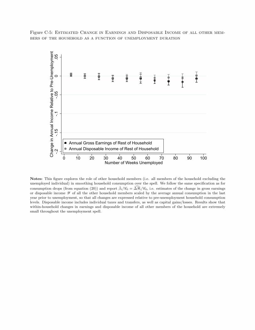
Figure C-5: Estimated Change in Earnings and Disposable Income of all other mem-bers of the household as a function of unemployment duration
-.2-.1
5-.1
-.05
0.0
5C
hang
e in
Ann
ual I
ncom
e R
elat
ive
to P
re-U
nem
ploy
men
t
0 10 20 30 40 50 60 70 80 90 100Number of Weeks Unemployed
Annual Gross Earnings of Rest of HouseholdAnnual Disposable Income of Rest of Household
Notes: This figure explores the role of other household members (i.e. all members of the household excluding theunemployed individual) in smoothing household consumption over the spell. We follow the same specification as for
consumption drops (from equation (20)) and report βt/C0 = ∆Yt/C0, i.e. estimates of the change in gross earningsor disposable income Y of all the other household members scaled by the average annual consumption in the lastyear prior to unemployment, so that all changes are expressed relative to pre-unemployment household consumptionlevels. Disposable income includes individual taxes and transfers, as well as capital gains/losses. Results show thatwithin-household changes in earnings and disposable income of all other members of the household are extremelysmall throughout the unemployment spell.
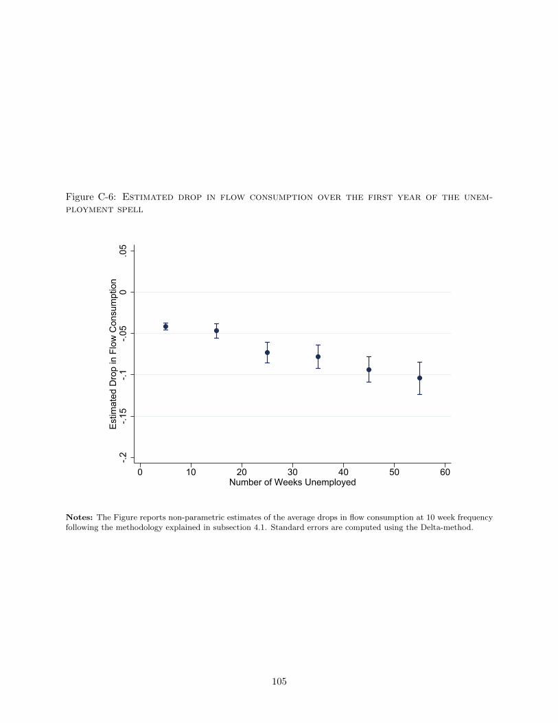
Figure C-6: Estimated drop in flow consumption over the first year of the unem-ployment spell
-.2-.1
5-.1
-.05
0.0
5Es
timat
ed D
rop
in F
low
Con
sum
ptio
n
0 10 20 30 40 50 60Number of Weeks Unemployed
Notes: The Figure reports non-parametric estimates of the average drops in flow consumption at 10 week frequencyfollowing the methodology explained in subsection 4.1. Standard errors are computed using the Delta-method.
105

Table C-1: Pre-unemployment characteristics of individuals with spells longer than20 weeks. Linear probability model estimates
(1) (2) (3) (4) (5)Duration of future spell ≥ 20 weeks
Age: 30 to 39 0.129*** 0.118*** 0.116*** 0.119*** 0.120***(0.00237) (0.00250) (0.00251) (0.00305) (0.00311)
Age: 40 to 49 0.164*** 0.153*** 0.153*** 0.162*** 0.163***(0.00277) (0.00293) (0.00295) (0.00357) (0.00363)
Age: 50+ 0.272*** 0.261*** 0.265*** 0.281*** 0.282***(0.00288) (0.00307) (0.00319) (0.00367) (0.00371)
Married 0.0289*** 0.0283*** 0.0287*** 0.0185*** 0.0190***(0.00243) (0.00243) (0.00244) (0.00280) (0.00281)
Gender: Female -0.00226 -0.00209 -0.00279 -0.0146*** -0.0135***(0.00192) (0.00193) (0.00193) (0.00230) (0.00230)
# of children -0.0329*** -0.0315*** -0.0288*** -0.0318*** -0.0311***(0.00193) (0.00193) (0.00193) (0.00231) (0.00233)
2nd quintile of income 0.0412*** 0.0436*** 0.0321*** 0.0319***(0.00319) (0.00319) (0.00409) (0.00412)
3rd quintile of income 0.0842*** 0.0885*** 0.0850*** 0.0849***(0.00319) (0.00319) (0.00403) (0.00415)
4th quintile of income 0.0471*** 0.0532*** 0.0532*** 0.0545***(0.00328) (0.00329) (0.00404) (0.00421)
5th quintile of income 0.0453*** 0.0518*** 0.0589*** 0.0635***(0.00341) (0.00345) (0.00411) (0.00431)
0<Net wealth≤200k -0.0503*** -0.0116*** -0.0122***(0.00234) (0.00271) (0.00315)
200k<Net wealth≤500k -0.0466*** -0.0146*** -0.0114***(0.00324) (0.00350) (0.00425)
500k<Net wealth≤5M -0.0186*** 0.00576* 0.00774*(0.00300) (0.00336) (0.00418)
Net wealth>5M 0.0731*** 0.0852*** 0.0866***(0.0173) (0.0172) (0.0174)
Fraction of portfolio in stocks
3rd quartile -0.000542(0.00787)
4th quartile 0.0303***(0.00259)
Leverage: debt / assets
2nd quartile 0.0153***(0.00390)
3rd quartile -0.0120***(0.00322)
4th quartile -0.00629*(0.00361)
R2 0.0465 0.0490 0.0511 0.0624 0.0620N 269931 269931 269931 190176 190176
Notes: The Table assesses the robustness of our welfare conclusions to dynamic selection on risk preferences over the un-employment spell. We investigate how various observable characteristics correlate with the probability to experience a longunemployment spell. To do so, we restrict the sample to all individuals about to become unemployed in the next quarter andestimate a linear probability model where the outcome is an indicator variable for experiencing a future spell longer than 20weeks. The default age category is 18 to 30 years old. Income refers to individual disposable income and results are relative tothe first quintile. Net wealth results are relative to individuals with zero or negative net wealth at the start of the spell. Wealso investigate the effect of two portfolio characteristics, that, conditional on net wealth, are traditionally correlated with riskpreferences. First, we look at the fraction of total wealth invested in stocks, and results are relative to the first two quartile ofthis distribution (50% of the sample have zero stocks prior to becoming unemployed). Second, we look at leverage defined astotal debt divided by gross assets, and results are relative to the first quartile of leverage.

C.4 Consumption profiles over the spell using household consumption surveys
(HUT)
In order to analyze the evolution of consumption as a function of time spent unemployed, we have also merged the
household consumption surveys (HUT) with the universe of administrative UI records. This enables us to reconstruct
the full employment history of individuals whose household is surveyed in the HUT. We observe employment status
of all individuals prior, during and after their HUT interview.
We restrict the sample to households where an individual is either unemployed at the time of the interview, or
who will become unemployed some time in the next two years following the interview. This leaves us with a pseudo-
panel of households for which we can correlate flow measures of consumption with time since (or until) the onset of
the unemployment spell. Note that this sample is a pseudo-panel and not a panel stricto sensu, as households are
surveyed only once in the HUT. However, because we observe the full unemployment history of individuals irrespective
of the time they are surveyed, we can fully control for selection issues arising from differences between households
who select into spells of different lengths.
In Table C-2, we provide summary statistics for unemployed individuals from the HUT sample. Unemployment
duration patterns are almost identical in the HUT sample and in the RKD sample, with an average duration of
unemployment of 26.6 weeks, and an average time spent in the first (resp. second) part of the profile of 12.9 weeks
(resp. 13.8 weeks). Average replacement rates are also identical at 72%. Interestingly, unemployed individuals
have similar demographics in the two samples. The distribution of age, gender, marital status and education levels
are almost identical. Average earnings are also similar in the two samples, but the distribution of earnings is by
construction much more spread out in the HUT sample than in the RKD sample, because the RKD sample is focused
on unemployed with daily wages in the neighborhood of 725SEK. Finally, the two samples have very comparable
distribution of assets and debts. In both samples, unemployed individuals have a household net wealth equal to 2.5
times their yearly earnings at the start of the spell. Overall, samples of unemployed individuals in the HUT and
RKD analysis are well-balanced in terms of all observable characteristics and unemployment durations.
We start by providing graphical evidence for the evolution of average consumption as a function of time spent
unemployed. We report in Figure C-7 the estimated coefficients βk from the regression model:
ci,t =
+4∑k=−3
βk · 1[t ∈ [26 ∗ k, 26 ∗ k + 1)] +X ′iγ + εi,t (28)
where ci,t is log household consumption in the HUT survey observed at the time of the HUT interview. t is event
time in weeks since the start of the unemployment spell. We aggregate event time in bins of 6 months periods (26
weeks), so that 1[t ∈ [26 ∗ k, 26 ∗ k + 1)] is an indicator for being observed in the k-th 6 months period since the
start of an unemployment spell.70 We include in this regression a set of controls X, which consists of year dummies,
calendar month dummies and a set of dummies for family status. The estimated coefficients βk plotted in Figure
C-7 represent the average log household consumption for households with an individual observed in her 26 ∗ k-th to
26 ∗ (k + 1)-th week of unemployment, relative to the average consumption level of households with an individual
observed just prior to becoming unemployed.
The graph provides strong evidence corroborating our findings from the registry-based measure of consumption,
that average household consumption drops significantly when unemployed. The average consumption of households
where a member has been unemployed for more than a year is almost 15% lower than prior to the unemployment
spell. Furthermore, Figure C-7 indicates that consumption declines significantly throughout the unemployment spell.
The consumption drop is still limited early on in the spell, but average consumption decreases sharply as duration
increases, and seems to be reaching a plateau after about a year in the unemployment spell. The last interesting
finding is the lack of anticipation prior to the unemployment spell. Household consumption is flat in the year
70k = 0 is the baseline and represents consumption in the last 6 months prior to becoming unemployed. HUTsurveys collect information on bi-weekly household consumption expenditures at the time of the interview. ci,t isthen annualized by multiplying bi-weekly consumption by 26.
107

preceding the onset of the unemployment spell. This also confirms evidence from the registry data and suggests that
unemployment shocks are relatively unanticipated, or that households have little propensity to change consumption
prior to becoming unemployed to smooth out the upcoming earnings shock.
To recover the average consumption drops in the first and second part of the unemployment spell and to investigate
the role of selection, we move in Table C-3 to a regression setting. In column (1), we start by running the simple
regression:
ci,t = η1 · 1[0 < t <= 20 wks] + η2 · 1[t > 20 wks] +X ′iγ + εi,t, (29)
where ci,t is log consumption of the household and η1 (resp. η2) captures the effect of having a member of the household
unemployed for less than 20 weeks (resp. more than 20 weeks) at the time of the interview, relative to households
where one individual will become unemployed in the next 6 months. The baseline specification reported in column (1)
controls for year dummies and calendar month dummies. Results suggest that relative to pre-unemployment levels,
total average household consumption drops by 6% in the first 20 weeks of unemployment, and by 13% after 20 weeks
of unemployment.
In column (2) of Table C-3, we add non-parametric controls for marital status, household size and age, and
find similar results with an initial drop of 4% in the first 20 weeks and 13% after 20 weeks of unemployment. In
columns (3) and (4), we analyze the role of selection in explaining these consumption patterns. If households with
long unemployment spells are inherently different from households with short unemployment spells, the estimated
drops in consumption after 20 weeks in column (1) and (2) may partly pick up these differences. To investigate such
selection effects, we estimate in column (3) a model of the form
ci,t = η1 · 1[0 < t <= 20 wks] + η2 · 1[t > 20 wks] + α · 1[L > 20 wks] +X ′iγ + εi,t, (30)
where 1[L > 20 wks] is a dummy variable for the completed length of the unemployment spell being longer than 20
weeks. In other words, because we observe in the UI records the total duration of each spell irrespective of the time
when the household is surveyed in the HUT, we can control for consumption differences at any point in time between
households with long versus short spells. Results indicate that between households who select into spells longer than
20 weeks versus households who select into spells shorter than 20 weeks, differences in log consumption levels are
small and not significant.
In column (4), we estimate not only differences in levels but also differences in consumption profiles between
households who select into spells longer than 20 weeks versus households who select into spells shorter than 20 weeks.
To do so, we fully interact 1[L > 20 wks] with the event time dummies to estimate two separate consumption profiles
over the unemployment spell: one for households with long spells and one for households with short spells. Results
reported in column (4) indicate that the consumption drop in the first 20 weeks for households who select into long
spells is 1.3% smaller but not statistically different from the consumption drop in the first 20 weeks of households
who select into short spells71. This evidence suggest that differences in consumption profiles are relatively small
and insignificant, so that selection effects are not significantly driving the observed patterns of average household
consumption over the unemployment spell.
Tables C-5 and C-6 replicate the analysis of, respectively, column 3 and 4 of Table C-3 for various categories of
consumption available in the HUT data. These tables are aimed at gauging how the difference between expenditures
and actual consumption may affect our conclusions regarding the evolution of consumption smoothing gains over the
unemployment spell, as explained in section 4.2 . The goal is to detect whether individuals who select into long versus
short spells have access to different means of smoothing consumption using substitution across different expenditure
categories. Results indicate that the expenditure levels and expenditure profiles over food, recreation, transportation,
or restaurants are not significantly different for households that select into long versus short spells. This suggests
that there is no significant dynamic selection over the spell based on the availability of substitution towards home
production. Equivalently, expenditure levels and expenditure profiles over durable goods are not significantly different
71To control for length-biased sampling, we also implemented all specifications using reweighting approaches, andwith more flexible controls for longer durations L. Results are identical, and available upon request.
108

for households that select into long versus short spells. The availability of consumption smoothing through shifting
expenditures away from durables is not significantly different for households that select into long versus short spells.72
Figure C-7: Log household consumption relative to last semester prior to the un-employment spell
-.4-.3
-.2-.1
0.1
Log
Con
sum
ptio
n
-104 -78 -52 -26 0 26 52 78Weeks relative to start of U spell
Notes: The figure correlates household consumption measured in the HUT survey with the time t since (or until) theonset of the unemployment spell observed in the administrative UI records. Bi-weekly household consumption levelsmeasured at the moment of the HUT interview are annualized and expressed in constant SEK2003. The figure followsfrom regression model (28) and plots the estimated coefficients βk for the set of indicators 1[t ∈ [26∗k, 26∗k+1)] forbeing observed in the k-th 6 months period since the onset of one’s spell. We also plot the 95% confidence interval fromrobust standard errors. We include in this regression a set of controls X, which consists of year dummies, calendarmonths dummies and a set of dummies for family status. The graph provides evidence that average householdconsumption drops over the unemployment spell. The average consumption of households where a member has beenunemployed for a full year is more than 15% lower than the average consumption of household with a member at thestart of her spell.
72It should be noted that the small sample size in the HUT offers limited statistical power and that it would beinteresting to get further evidence on these various expenditure patterns.
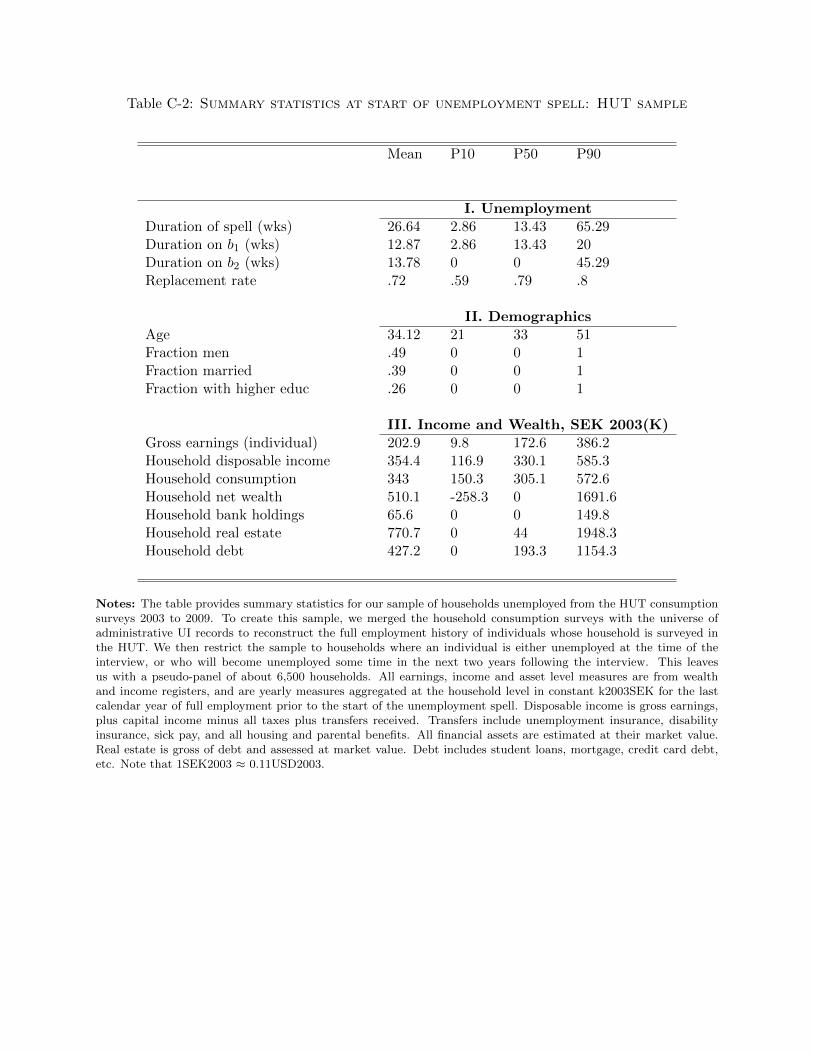
Table C-2: Summary statistics at start of unemployment spell: HUT sample
Mean P10 P50 P90
I. UnemploymentDuration of spell (wks) 26.64 2.86 13.43 65.29Duration on b1 (wks) 12.87 2.86 13.43 20Duration on b2 (wks) 13.78 0 0 45.29Replacement rate .72 .59 .79 .8
II. DemographicsAge 34.12 21 33 51Fraction men .49 0 0 1Fraction married .39 0 0 1Fraction with higher educ .26 0 0 1
III. Income and Wealth, SEK 2003(K)Gross earnings (individual) 202.9 9.8 172.6 386.2Household disposable income 354.4 116.9 330.1 585.3Household consumption 343 150.3 305.1 572.6Household net wealth 510.1 -258.3 0 1691.6Household bank holdings 65.6 0 0 149.8Household real estate 770.7 0 44 1948.3Household debt 427.2 0 193.3 1154.3
Notes: The table provides summary statistics for our sample of households unemployed from the HUT consumptionsurveys 2003 to 2009. To create this sample, we merged the household consumption surveys with the universe ofadministrative UI records to reconstruct the full employment history of individuals whose household is surveyed inthe HUT. We then restrict the sample to households where an individual is either unemployed at the time of theinterview, or who will become unemployed some time in the next two years following the interview. This leavesus with a pseudo-panel of about 6,500 households. All earnings, income and asset level measures are from wealthand income registers, and are yearly measures aggregated at the household level in constant k2003SEK for the lastcalendar year of full employment prior to the start of the unemployment spell. Disposable income is gross earnings,plus capital income minus all taxes plus transfers received. Transfers include unemployment insurance, disabilityinsurance, sick pay, and all housing and parental benefits. All financial assets are estimated at their market value.Real estate is gross of debt and assessed at market value. Debt includes student loans, mortgage, credit card debt,etc. Note that 1SEK2003 ≈ 0.11USD2003.

Table C-3: Household log-consumption as a function of time spent unemployed rel-ative to pre-unemployment consumption: consumption survey estimates
(1) (2) (3) (4)
1[0 < t ≤ 20 weeks] (η1) -0.0606* -0.0444 -0.0408 -0.0465(0.0316) (0.0311) (0.0314) (0.0413)
1[t > 20 weeks] (η2) -0.130*** -0.129*** -0.111*** -0.108***(0.0328) (0.0332) (0.0386) (0.0414)
1[L > 20 weeks] -0.0294 -0.0342(0.0308) (0.0378)
1[0 < t ≤ 20 weeks]× 1[L > 20 weeks] 0.0134(0.0629)
Year F-E × × × ×Calendar months F-E × × × ×Marital status × × ×Family size × × ×Age group F-E × × ×
Test η1 = η2P-value 0.06 0.02 0.08 0.10
R2 0.0493 0.0866 0.0872 0.0872N 1551 1548 1548 1548
Notes: Robust standard errors in parentheses. * p<.10, ** p<.05, *** p<.01.The Table reports estimates of the drop in household consumption over the unemployment spell in the HUT surveys,following model of equation (29). Because the HUT surveys collect information on household consumption expen-ditures at the time of the interview, HUT estimates can directly recover flow (bi-weekly) measures of consumptionct. We restrict the sample to households where, at the date of the interview, one (and only one) individual is unem-ployed, or where, at the date of the interview, one (and only one) individual will become unemployed in the following6 months. 1[0 < t <= 20 weeks] is an indicator for having a member of the household unemployed since less than 20weeks at the time of the interview. 1[t > 20 weeks] is an indicator for having a member of the household unemployedfor more than 20 weeks at the time of the interview. 1[L > 20 weeks] is an indicator for the total duration of theunemployment spell being longer than 20 weeks. We also report the P-value of a test of equality of η1 (the drop inconsumption in the first 20 wks) and η2 (the drop in consumption after 20 wks).
111

Table C-4: Consumption as a function of time spent unemployed relative to pre-unemployment consumption:consumption survey estimates for various expenditure categories
(1) (2) (3) (4) (5) (6) (7) (8)Total Food Rents Purchase Furniture Trans- Recre- Restau-
expenditures of new & house portation ation rantvehicles appliances
1[0 < t ≤ 20 weeks] -0.0606* -0.0441 -0.0404 -0.418** -0.160 -0.0788 -0.106 -0.0807(0.0316) (0.0388) (0.0380) (0.187) (0.102) (0.0661) (0.0649) (0.0876)
1[t > 20 weeks] -0.130*** -0.0823* 0.0430 -0.252 -0.0883 -0.348*** -0.189*** -0.165*(0.0328) (0.0441) (0.0310) (0.176) (0.0884) (0.0803) (0.0719) (0.0888)
Year fixed effects × × × × × × × ×Calendar months F- E × × × × × × × ×
R2 0.0493 0.0650 0.0365 0.0205 0.00975 0.0208 0.0252 0.0154N 1551 1548 798 982 1548 1488 1543 1119
Notes: Robust standard errors in parentheses. * p<.10, ** p<.05, *** p<.01.The Table reports estimates of the drop in household consumption over the unemployment spell in the HUT surveys, following model of equation (29). Becausethe HUT surveys collect information on household consumption expenditures at the time of the interview, HUT estimates can directly recover flow (bi-weekly)measures of consumption ct. We restrict the sample to households where, at the date of the interview, one (and only one) individual is unemployed, or where, atthe date of the interview, one (and only one) individual will become unemployed in the following 6 months. 1[0 < t <= 20 weeks] is an indicator for having amember of the household unemployed since less than 20 weeks at the time of the interview. 1[t > 20 weeks] is an indicator for having a member of the householdunemployed for more than 20 weeks at the time of the interview. 1[L > 20 weeks] is an indicator for the total duration of the unemployment spell being longerthan 20 weeks.
112

Table C-5: Log-consumption as a function of time spent unemployed relative to pre-unemployment consumption:consumption survey estimates for various expenditure categories, selection on levels
(1) (2) (3) (4) (5) (6) (7) (8)Total Food Rents Purchase Furniture Trans- Recre- Restau-
expenditures of new & house portation ation rantvehicles appliances
1[0 < t ≤ 20 weeks] -0.0379 -0.0139 -0.0212 -0.192 -0.0657 -0.0596 -0.0948 -0.0765(0.0305) (0.0366) (0.0368) (0.172) (0.0893) (0.0658) (0.0649) (0.0876)
1[t > 20 weeks] -0.113*** -0.0782* 0.0143 -0.387* -0.0463 -0.330*** -0.146* -0.141(0.0379) (0.0463) (0.0356) (0.217) (0.102) (0.0925) (0.0850) (0.104)
1[L > 20 weeks] -0.0294 -0.00917 0.0239 0.0106 -0.0394 -0.0223 -0.0775 -0.0208(0.0300) (0.0364) (0.0312) (0.159) (0.0848) (0.0659) (0.0654) (0.0811)
Year fixed effects × × × × × × × ×Marital status × × × × × × × ×Family size × × × × × × × ×
R2 0.139 0.194 0.157 0.0686 0.0442 0.0525 0.0567 0.0369N 1548 1545 796 606 1523 1485 1540 1116
Notes: Robust standard errors in parentheses. * p<.10, ** p<.05, *** p<.01.The Table reports estimates of the drop in household consumption over the unemployment spell in the HUT surveys, following model of equation (29). Becausethe HUT surveys collect information on household consumption expenditures at the time of the interview, HUT estimates can directly recover flow (bi-weekly)measures of consumption ct. We restrict the sample to households where, at the date of the interview, one (and only one) individual is unemployed, or where, atthe date of the interview, one (and only one) individual will become unemployed in the following 6 months. 1[0 < t <= 20 weeks] is an indicator for having amember of the household unemployed since less than 20 weeks at the time of the interview. 1[t > 20 weeks] is an indicator for having a member of the householdunemployed for more than 20 weeks at the time of the interview. 1[L > 20 weeks] is an indicator for the total duration of the unemployment spell being longerthan 20 weeks.
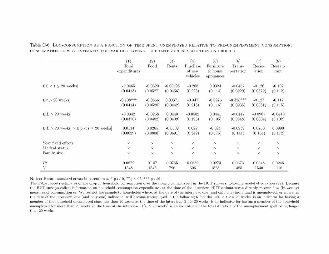
Table C-6: Log-consumption as a function of time spent unemployed relative to pre-unemployment consumption:consumption survey estimates for various expenditure categories, selection on profile
(1) (2) (3) (4) (5) (6) (7) (8)Total Food Rents Purchase Furniture Trans- Recre- Restau-
expenditures of new & house portation ation rantvehicles appliances
1[0 < t ≤ 20 weeks] -0.0465 -0.0320 -0.00595 -0.288 0.0324 -0.0457 -0.126 -0.107(0.0413) (0.0527) (0.0456) (0.223) (0.114) (0.0920) (0.0879) (0.112)
1[t > 20 weeks] -0.108*** -0.0666 0.00371 -0.347 -0.0976 -0.328*** -0.127 -0.117(0.0414) (0.0528) (0.0442) (0.218) (0.116) (0.0935) (0.0881) (0.115)
1[L > 20 weeks] -0.0342 -0.0258 0.0440 -0.0582 0.0441 -0.0147 -0.0967 -0.0410(0.0378) (0.0482) (0.0409) (0.193) (0.105) (0.0848) (0.0804) (0.102)
1[L > 20 weeks]× 1[0 < t ≤ 20 weeks] 0.0134 0.0265 -0.0509 0.022 -0.024 -0.0239 0.0750 0.0990(0.0629) (0.0800) (0.0691) (0.342) (0.175) (0.141) (0.134) (0.172)
Year fixed effects × × × × × × × ×Marital status × × × × × × × ×Family size × × × × × × × ×
R2 0.0872 0.107 0.0765 0.0689 0.0273 0.0373 0.0348 0.0246N 1548 1545 796 606 1523 1485 1540 1116
Notes: Robust standard errors in parentheses. * p<.10, ** p<.05, *** p<.01.The Table reports estimates of the drop in household consumption over the unemployment spell in the HUT surveys, following model of equation (29). Becausethe HUT surveys collect information on household consumption expenditures at the time of the interview, HUT estimates can directly recover flow (bi-weekly)measures of consumption ct. We restrict the sample to households where, at the date of the interview, one (and only one) individual is unemployed, or where, atthe date of the interview, one (and only one) individual will become unemployed in the following 6 months. 1[0 < t <= 20 weeks] is an indicator for having amember of the household unemployed since less than 20 weeks at the time of the interview. 1[t > 20 weeks] is an indicator for having a member of the householdunemployed for more than 20 weeks at the time of the interview. 1[L > 20 weeks] is an indicator for the total duration of the unemployment spell being longerthan 20 weeks.

FOR ONLINE PUBLICATION - Appendix D: Structural Welfare
Analysis
This Appendix provides more detail on the specification, approach and results of our calibration exercise.
D.1 Calibration
Our structural model builds on the search environment considered in Hopenhayn and Nicolini [1997], Lentz and
Traneas [2005] and Chetty [2008a]. We consider agents with CRRA preferences with additive, iso-elastic search costs,
vui,t (ci,t, si,t) = c1−γi,t / (1− γ)− ψ0 (si,t)ψ1 ,
vei,t (ci,t) = c1−γi,t / (1− γ) .
In contrast with the previous models, we allow for individual-specific, duration-dependent exit rate functions
hi,t (si,t) = h0 + [1 + exp (−θt)]κih1 × sρi,t,
where h1 determines the return to search, θ is the exponential rate at which these returns depreciate, κi is an
individual-specific scalar, drawn from a gamma distribution Γ (a, b) , and h0 is a baseline exit rate (at zero effort).
Each household starts the unemployment spell with an asset level ai,1, drawn from a Singh-Maddala distribution
F (a|αSM , cSM , kSM ) (Singh and Maddala [1976]). Each household can draw down their asset to increase consumption
as long as ai,t ≥ a, where a is a uniform asset limit. We choose the distribution parameters to match the average,
25-th and 90-th percentile of the household distribution of liquid assets.
We consider a flat benefit policy that replaces 72% of the pre-unemployment earnings, normalized to 1. When
employed, the agent pays a (uniform) tax τ equal to 5%, which balances the expected revenues and expenditures
for the average Swedish unemployment rate between 1999 and 2006 of .069. Our calibration targets household
consumption levels, we therefore augment the individual’s income with a household income of .7, which corresponds
to the average share of other household members’ earnings relative to the earnings of the unemployed in our sample
(see Table 2).
We set the parameter of CRRA γ = 2, discount factor β = 1 and interest rate r = 0. All other parameters are
used to calibrate the model. We solve the model using an asset grid of 500 grid points and 10 different deciles of
the distribution of individual-specific returns to search. For each decile we solve the model backwards starting in
week T = 520 and then simulate the economy forward for each asset level. We then aggregate up the time paths for
consumption and the survival rates using the joint distribution over assets and individual-specific returns to search.
We compute the elasticities and average durations implied by the model.
D.2 Model Fit
Table D-1 lists the targets of the calibration, which are the variables underlying our sufficient statistics. The targets
include the benefit duration elasticities εD,bk , average benefit durations Dk and the average consumption drops
[ck − c0] /c0. The benchmark consumption level c0 is the average level of consumption when agents would have been
employed from the start of the model. For each of the target variables, we target the level for the first part of the policy,
as well as the ratio for the two parts and we put higher weight on the latter. Our minimization routine searches for
the vector of parameter values that minimizes the relative difference between the targeted moments and the simulated
values of these moments generated by our model and is robust to different starting values for the parameters. Table D-1
compares the targeted and estimates values of these moments. The calibration slightly overestimates the consumption
drop in the first 20 weeks and underestimates the consumption drop thereafter. The simulated drops are well within
the 95% confidence intervals of our empirical estimates, but imply that we underestimate the CS2/CS1 compared
to our sufficient-statistics implementation. Our calibrated model also underestimates the unemployment durations
and elasticities, but closely matches the relative moral hazard costs MH2/MH1. The model underestimates the
115

unemployment durations and elasticities, but matches the ratios very well. The calibrated parameters for the returns
to search imply both strong depreciation of the exit rates and heterogeneity in exit rates. The average exit rate
equals .21 in the first week of the spell and .03 in the 20-th week of unemployment, while the exit rate of a given job
seeker is about half as large in the 20-th week compared to the first week. The model also predicts that 53% of the
unemployed are liquidity constrained and consume hand-to-mouth from the start of the unemployment spell.
Table D-1: Model Calibration: Targeted and Estimated values
Targets Description Targeted EstimatedValue Value
a.25 25th percentile of asset distribution 0.00 0.000a.90 90th percentile of asset distribution 0.42 0.553amean mean of asset distribution 0.19 0.203∆c1 consumption drop ST unemployed 0.060 0.072
∆c1/∆c2 ratio of consumption drops 0.462 0.658D1 ST benefit duration 12.600 6.675
D1/D2 ratio of benefit duration 0.940 0.991εDb1 elasticity wrt ST benefits 0.854 0.549
εDb1 /εDb2 ratio of elasticities 1.262 1.271
Notes: The table lists the variables we target in our calibration exercise. These are the moments underlying oursufficient statistics such that the structural model provides the same policy recommendations as implied by thesufficient-statistics approach. For each of the target variables, we target the level for the first part of the policy,as well as the ratio for the two parts. The parameters of the asset distribution are set to match the mean, 25-thand 90-th percentile of the household distribution of liquid assets (expressed relative to annual household income).We also set the parameter of CRRA γ = 2, discount factor β = 1 and interest rate r = 0. The remaining modelparameters are calibrated to minimize the relative distance between the targeted moments and the simulated valuesof these moments generated by our model.
116

D.3 Counterfactual Analysis
The calibrated model allows analyzing the moral hazard costs and consumption smoothing gains for different unem-
ployment policies, keeping all parameters constant, including the asset distribution at the start of the unemployment
spell. The government’s budget is affected by the changes in the benefit levels (as we keep the tax rate fixed), but
these budgetary changes are traded off against the agents’ welfare, using the normalization of the Lagrange multiplier
on the government’s constraint, λ ≡ E0 (v′ (ci,0)), where ci,0 is the agent’s level of consumption when she would have
been employed from the start of the model. Figure 7 plots the respective consumption smoothing gains and moral
hazard costs. CSb and MHb have a unique intersection for b = .58, which corresponds to the optimal flat benefit
level for the given tax rate and Lagrange multiplier. Similarly, we find that CS1 = MH1 and CS2 = MH2 jointly
hold for the unique pair (b1, b2) = (.48, .68).
We repeat the previous analysis for two variations of our baseline model. In the model with only heterogeneity
in the returns to search, we set the search depreciation parameter θ = 0, but re-calibrate the return to search
parameter h1 to maintain the same average duration. All other parameters remain the same. In the model with only
depreciation of the returns to search, we assume a uniform scalar κi = κ and re-calibrate h1 to maintain the same
average duration. Figure D-1 illustrates the respective consumption smoothing gains and moral hazard costs. The
simulated implications for the flat profile are similar, except that the unemployment elasticities and thus the moral
hazard costs are higher in the model with only depreciation (but no heterogeneity). In both alternative models,
MHb decreases while CSb increases when the replacement rate is reduced. They are equalized for b = .60 in the
model with only heterogeneity and b = .40 in the model with only depreciation. Regarding the tilt, the model with
only depreciation of exit rates increases MH2 relative to MH1.73 This calibration pushes towards a declining tilt
and more so as the overall generosity is reduced. However, the model with only heterogeneity continues to prescribe
an inclining tilt and this remains true for lower replacement rates. Importantly, conditional on the values of the
sufficient statistics, the underlying depreciation and heterogeneity do not affect the local policy recommendations.
The differential impact on how the sufficient statistics change with the unemployment policy, however indicates the
complementary value of a structural approach and disentangling the two non-stationary forces to go beyond our local
recommendations.
We also note that the structural model can be exploited to assess the potential importance of some implementation
assumptions. We simulate the consumption drops and calculate the implied consumption smoothing gains for different
levels of risk aversion, reported in Table D-2, while keeping all other parameters constant. The Taylor approximation
of the marginal CRRA utilities tends to underestimate the consumption smoothing gains, especially when the level of
risk aversion is high. This was already noted in Chetty [2006]. Interestingly, the approximation error on the relative
consumption smoothing gains is very small and thus the recommendation on the tilt unaffected, regardless of the
level of risk aversion.
We finally use the structural model to gauge the impact of heterogeneity in preferences on the estimated con-
sumption smoothing gains. We simulate a model with share α of job seekers with risk aversion γ = 1 and share
1 − α with risk aversion γ = 3. We set α = .58 such that the average risk aversion among the unemployed, ac-
counting for type-specific unemployment durations, equals γ = 2. Since the consumption drops hardly change for
agents with different preferences, the average consumption drops in the model with heterogeneity remain very similar
compared to the baseline model. The dynamic selection on preferences could in principle affect the relative consump-
tion smoothing gains, as shown in subsection 5.2.3. Note that in our model with CRRA preferences and additive
search cost (a standard specification also used in Hopenhayn and Nicolini [1997] and Chetty [2008a]), individuals
with higher risk aversion have lower marginal utility of consumption (relative to the disutility of search), therefore
search less and leave unemployment more slowly. As illustrated in equation (21) in subsection 1.3, dynamic selec-
tion on both the marginal utility of consumption Ek [v′i (ci,0)] /E0 [v′i (ci,0)] and the consumption smoothing gains
Ek[v′′i (ci,0)
(ci,0 − cui,t
)]/E0 [v′i (ci,0)] affect the value of CSk. Hence, the net impact is ambiguous. In our simula-
tion with heterogeneity, the aggregate consumption smoothing gains CS1 and CS2 are lower relative to the baseline
73Note that in Appendix C we demonstrated that depreciation in the search returns can increase MH1 relative toMH2. This comparative static was derived without keeping the average duration constant.
117

scenario. The ratio CS1/CS2 decreases as well, which further increases the value of introducing an inclining tilt
(b2 > b1). We note though that with heterogeneous preferences, the calculation of CSk critically depends on the
normalization λ ≡ E0 (v′ (ci,0)). We can avoid this normalisation by directly considering the relative consumption
smoothing gains [1 + CS1] / [1 + CS2] = E1 (v′i (ci,t)) /E2 (v′i (ci,t)), relevant for evaluating a budget-balanced change
in the tilt. This ratio changes from .934 in the baseline calibration to .935 in the simulation with heterogeneity (cf.
Table D-2) Overall, the introduction of preference heterogeneity seems to limited impact on the relative consumption
smoothing gains in our simulations and, if anything, increases the welfare gain from introducing an inclining tilt
(b2 > b1).
118

Figure D-1: Alternative Model Specifications: Welfare Effects for Different Ben-efit Levels
A. Only heterogeneity in returns to search
Actual flat policy
Optimal flat policy
0.5
11.
52
2.5
MH,
MH k,
CS, C
S k
.2 .3 .4 .5 .6 .7 .8(flat) replacement rate
MH MH1 MH2
CS CS1 CS2
B. Only depreciation of returns to search
Actual flat policy
Optimal flat policy
02
46
8M
H, M
H k, CS
, CS k
.2 .3 .4 .5 .6 .7 .8(flat) replacement rate
MH MH1 MH2
CS CS1 CS2
Notes: The figure analyzes the robustness of the findings in Figure 7 for different model specifications. The twopanels plot the moral hazard costs and consumption smoothing gains for different levels of the flat benefit profile.Panel A uses a model without depreciation of the returns to search and only heterogeneity in the returns to search.Panel B uses a model with only depreciation of the returns to search and no heterogeneity in the returns to search.Compared to our baseline model, we re-calibrate the uniform return to search parameter to maintain the same averageexit rate. The actual policy is a flat profile with average replacement rate of .72 and is indicated by the verticaldashed line. We report the simulated moral hazard costs and consumption smoothing gains for an overall change inthe flat benefit profile b, for an increase in the benefit level in the first 20 weeks of unemployment, and for an increasein the benefit level after 20 weeks of unemployment.
119

Table D-2: Implementation of consumption smoothing gains
Consumption Smoothing Gain
∆ck/c Ek [v′i (ci,t)] CSk γ∆ck/c
Baseline Calibration: γ=2
Throughout spell 0.091 0.443 0.231 0.181First 20 weeks 0.072 0.428 0.189 0.143After 20 weeks 0.109 0.458 0.273 0.218
Before 20wks / after 20 wks 0.658 0.934 0.693 0.658
Simulation with heterogenous preferences
Throughout spell 0.091 0.485 0.108 0.182First 20 weeks 0.072 0.469 0.070 0.144After 20 weeks 0.109 0.501 0.144 0.217
Before 20wks / after 20 wks 0.664 0.935 0.483 0.664
Simulation with low risk aversion γ=1
Throughout spell 0.093 0.666 0.109 0.093First 20 weeks 0.074 0.653 0.088 0.074After 20 weeks 0.112 0.677 0.129 0.112
Before 20wks / after 20 wks 0.658 0.964 0.682 0.658
Simulation with high risk aversion γ=3
Throughout spell 0.088 0.296 0.368 0.264First 20 weeks 0.071 0.282 0.307 0.212After 20 weeks 0.105 0.309 0.429 0.316
Before 20wks / after 20 wks 0.671 0.914 0.715 0.671
Notes: This Table illustrates alternative implementations of the consumption smoothing gains for different underlyingrisk preferences. The top panel reports the simulated consumption drops and consumption smoothing gains for thebaseline model with homogeneous CRRA γ=2. The third and fourth panel report the simulated values for lower CRRAγ=1 and higher CRRA γ=3, but still assuming homogenous preferences. The second panel reports the simulatedvalues for a model with a mixture of these two preference types, keeping the average CRRA among the unemployedequal to 2. This makes the results comparable to the baseline model. The first column in each panel shows thedrops in consumption during the respective parts of the unemployment spell relative to the consumption levels whenemployed at the start of the model. The second column shows the average marginal utility of consumption duringthe respective parts of the unemployment spell. The third column reports CSk, which expresses the average marginalutility of consumption in the second column relative to the average marginal utility of employment consumptionat the start of the model. The fourth column provides an approximation of CSk following the implementation in(14), which relies on a Taylor approximation and homogeneous preferences. For this fourth column, the second panelwith heterogeneous preferences simply multiplies the consumption drops by γ=2. The rows of each panel report theconsumption drops and consumption smoothing gains over the full unemployment spell, during the first 20 weeks ofunemployment and after 20 weeks of unemployment respectively. The last row shows the ratio of the first part to thesecond part of the unemployment spell.
120

References -Appendix A to Appendix D
Aguiar, Mark and Erik Hurst, “Consumption versus Expenditure,” Journal of Political Economy, 2005, 113 (5), pp.
919–948.
Andrews, Isaiah and Conrad Miller, “Optimal Social Insurance with Heterogeneity,” Mimeo, MIT, 2013.
Baily, Martin N., “Some Aspects of Optimal Unemployment Insurance,” Journal of Public Economics, 1978, 10 (3),
379–402.
Browning, Martin and Søren Leth-Petersen, “Imputing consumption from income and wealth information,” The
Economic Journal, 2003, 113 (488), F282–F301.
Card, David, David S. Lee, Zhuan Pei, and Andrea Weber, “Inference on Causal Effects in a Generalized Regression
Kink Design,” Econometrica, 2015, 83 (6), 2453–2483.
Chetty, Raj, “A General Formula for the Optimal Level of Social Insurance,” Journal of Public Economics, 2006, 90
(10-11), 1879–1901.
, “Moral Hazard versus Liquidity and Optimal Unemployment Insurance,” Journal of Political Economy, 2008,
116 (2), 173–234.
, “Sufficient Statistics for Welfare Analysis: A Bridge Between Structural and Reduced-Form Methods,” Annual
Review of Economics, 05 2009, 1 (1), 451–488.
and Adam Szeidl, “Consumption Commitments and Risk Preferences,” The Quarterly Journal of Economics,
2007, 122 (2), pp. 831–877.
and Amy Finkelstein, “Chapter 3 - Social Insurance: Connecting Theory to Data,” in Martin Feldstein Alan
J. Auerbach, Raj Chetty and Emmanuel Saez, eds., handbook of public economics, vol. 5, Vol. 5 of Handbook of
Public Economics, Elsevier, 2013, pp. 111 – 193.
Cohen, Alma and Liran Einav, “Estimating Risk Preferences from Deductible Choice,” American Economic Review,
2007, 97 (3), 745–788.
den Berg, Gerard Van, “Nonstationarity in Job Search Theory,” The Review of Economic Studies, 1990, 57 (2),
255–277.
Eckstein, Zvi and Gerard Van den Berg, “Empirical labor search: A survey,” Journal of Econometrics, 2007, 136 (2),
531 – 564. The interface between econometrics and economic theory.
Eika, L., M. Mogstad, and O. Vestad, “”What Can We Learn About Household Consumption From Information on
Income and Wealth”,” working paper, 2017.
Ganong, Peter and Simon Jaeger, “A Permutation Test and Estimation Alternatives for the Regression Kink Design,”
Harvard University Discussion Paper, 2014.
Gruber, Jonathan, “The Consumption Smoothing Benefits of Unemployment Insurance,” American Economic Review,
1997, 87 (1), 192–205.
Hendren, Nathaniel, “The Policy Elasticity,” Working Paper 19177, National Bureau of Economic Research June
2013.
Hopenhayn, Hugo A. and Juan Pablo Nicolini, “Optimal Unemployment Insurance,” Journal of Political Economy,
1997, 105 (2), 412–438.
Koijen, Ralph, Stijn Van Nieuwerburgh, and Roine Vestman, Judging the Quality of Survey Data by Comparison with
Truth as Measured by Administrative Records: Evidence From Sweden, University of Chicago Press, July 2014
Kolsrud, Jonas, Camille Landais, and Johannes Spinnewijn, “Registry-Based Measures of Consumption And Con-
sumption Patterns: What Can We Learn From the Swedish Administrative Data?,” Mimeo, 2017.
Kreiner, Claus T., David Dreyer Lassen, and Søren Leth-Petersen, “Liquidity Constraint Tightness and Consumer
Responses to Fiscal Stimulus Policy,” Mimeo, Copenhagen University, 2014.
Kroft, Kory and Matthew J Notowidigdo, “Should unemployment insurance vary with the unemployment rate?
121

Theory and evidence,” The Review of Economic Studies, 2016, p. rdw009.
, Fabian Lange, and Matthew J. Notowidigdo, “Duration Dependence and Labor Market Conditions: Evidence
from a Field Experiment,” The Quarterly Journal of Economics, 2013.
Krueger, Alan B. and Bruce D. Meyer, “Labor Supply Effects of Social Insurance,” Handbook of Public Economics,
Elsevier 2002.
Landais, Camille, “Assessing the Welfare Effects of Unemployment Benefits Using the Regression Kink Design,”
American Economic Journal: Economic Policy, 2015.
, Pascal Michaillat, and Emmanuel Saez, “Optimal Unemployment Insurance over the Business Cycle,” Working
Paper 16526, National Bureau of Economic Research 2010.
Lentz, Rasmus and Torben Traneas, “Job Search and Savings: Wealth Effects and Duration Dependence,” Journal
of Labor Economics, July 2005, 23 (3), 467–490.
Machin, Stephen and Alan Manning, “The Causes and Consequences of Longterm Unemployment in Europe,” in
Orley C. Ashenfelter and David Card, eds., Orley C. Ashenfelter and David Card, eds., Vol. 3, Part C of Handbook
of Labor Economics, Elsevier, 1999, pp. 3085 – 3139.
Mas, Alexandre and Andrew Jonhston, “Potential Unemployment Insurance Duration and Labor Supply: the Indi-
vidual and Market-Level Response to a Benefit Cut,” Mimeo, Princeton University, 2015.
McCrary, Justin, “Manipulation of the Running Variable in the Regression Discontinuity Design: A Density Test,”
Journal of Econometrics, February 2008, 142 (2), 698–714.
Meyer, Bruce, “Unemployment Insurance and Unemployment Spells,” Econometrica, 1990, 58(4), 757–782.
Mogstad, Magne and Andreas Kostol, “Earnings, Income, and Consumption of Alowed and Rejected Disability
Insurance Applicants,” American Economic Review, Papers and Proceedings, 2015, 105 (5), 137–141.
Nekoei, Arash and Andrea Weber, “Does Extending Unemployment Benefits Improve Job Quality?,” IZA Discussion
Papers 9034, Institute for the Study of Labor (IZA) April 2015.
Pavoni, Nicola, “Optimal Unemployment Insurance, With Human Capital Depreciation, and Duration Dependence,”
International Economic Review, 2009, 50 (2), 323–362.
Pistaferri, Luigi, “Household Consumption: Research Questions, Measurement Issues, and Data Collection Strate-
gies,” Mimeo Stanford University, 2015.
Rothstein, Jesse, “Unemployment Insurance and Job Search in the Great Recession,” Working Paper 17534, National
Bureau of Economic Research October 2011.
, , and , “The Effects of Extended Unemployment Insurance Over the Business Cycle: Evidence from Re-
gression Discontinuity Estimates Over 20 Years,” The Quarterly Journal of Economics, 2012, 127 (2), 701–752.
Shavell, Steven and Laurence Weiss, “The Optimal Payment of Unemployment Insurance Benefits over Time,” Journal
of Political Economy, 1979, 87 (6), 1347–1362.
and Ivan Werning, “On the Optimal Timing of Benefits with Heterogeneous Workers and Human Capital Depre-
ciation ,” 2006.
and , “Reservation Wages and Unemployment Insurance,” Quarterly Journal of Economics, 2007, 122 (3),
1145–1185.
and , “Liquidity and Insurance for the Unemployed,” American Economic Review, 2008, 98 (5), 1922–42.
Singh, S. and G. Maddala, “A Function for the Size Distribution of Incomes,” Econometrica, 1976, 44 (5), 963–970.
Spinnewijn, Johannes, “Unemployed but Optimistic: Optimal Insurance Design with Biased Beliefs,” Journal of the
European Economic Association, 2015, 13 (1), 130–167.
Valletta, Robert and Henry S. Farber, “Extended Unemployment Insurance and Unemployment Duration in The
Great Recession: The U.S. Experience,” Mimeo, Princeton University, 2011.
122

Werning, Ivan, “Optimal Unemployment Insurance with Unobservable Savings,” University of Chicago and UTDT,
2002.
123