The Optimal Scope of the Royalty Base in PatentLicensing∗

Gerard LlobetCEMFI and CEPR

Jorge PadillaCompass Lexecon

First draft: March 2014

This version: May 9, 2014

Abstract

There is considerable controversy about the relative merits of the apportionmentrule (which results in per-unit royalties) and the entire market value rule (whichresults in ad-valorem royalties) as ways to determine the scope of the royalty basein licensing negotiations and disputes. This paper analyzes the welfare implicationof the two rules abstracting from implementation and practicability considerations.We show that ad-valorem royalties tend to lead to lower prices, particularly in thecontext of successive monopolies. They benefit upstream producers but not neces-sarily hurt downstream producers. When we endogenize the investment decisions,we show that a sufficient condition for ad-valorem royalties to improve social welfareis that enticing more upstream investment is optimal or when multiple innovatorscontribute complementary technologies. Our findings contribute to explain whymost licensing contracts include royalties based on the value of sales.

JEL codes: L15, L24, O31, O34.keywords: Intellectual Property, Standard Setting Organizations, Patent Licensing,R&D Investment.

∗The ideas and opinions in this paper, as well as any errors, are exclusively the authors’. Financialsupport from Qualcomm is gratefully acknowledged. Comments should be sent to llobet@cemfi.es andjpadilla@compasslexecon.com.

1

1 Introduction

The licensing of a patented technology is one of the most important sources of revenue

for many innovators, particularly, when they do not participate in the production in the

final market. A licensing contract typically includes a royalty payment that comprises two

components: a royalty rate and a royalty base. Most attention in the economic literature

has been devoted to the optimal determination of the royalty rate. Much less work has

been done in studying the scope of the royalty base. This scope can be determined

in two principal ways. One option is the value of the components of the infringing

product that incorporate the patented technology. This is the so-called apportionment

rule. Alternatively, the scope of the royalty base can be given by the value of the sales of

the entire product – the entire market value rule. These two rules give raise to the usage

of per-unit royalty rates (a constant payment based on the units sold) and ad-valorem

royalty rates (a payment comprising a percentage of the value of the sales of the product),

respectively.

There is wide agreement among practitioners and legal scholars that the “entire mar-

ket value rule” is appropriate when the components incorporating the patented technology

drive the demand for the product. There is also wide agreement that in a perfect world

with rational judges and juries and in the absence of reporting and monitoring frictions,

both rules would produce the same payment outcomes even if the components incorpo-

rating the patented technology do not drive the demand for the product.1 The argument

is that in a frictionless world “the individual elements of a royalty payment are irrelevant

in isolation, as one variable [i.e. the royalty rate] can adjust with the other [i.e. the

royalty base].”2

1As stated by the U.S. Court of Appeals to the Federal Circuit (CAFC) “there is nothing inherentlywrong with using the market value for the entire product for the infringing component or feature, solong as the multiplier accounts for the proportion of the base represented by the infringing componentor feature.” Lucent Techs., Inc. v. Gateway, Inc., 580 F. 3d 1301, 1338-39 (Fed. Cir. 2009).

2See Geradin and Layne-Farrar (2011).

2

In contrast, there is considerable controversy about the appropriate rule for the de-

termination of the scope of the royalty base when that the components incorporating

the patented technology do not drive the demand for the product and there is bounded

rationality and/or asymmetries of information. In those circumstances, some scholars

support the apportionment rule because they fear that a royalty base that is broader

than the value of the components incorporating the technology may mislead judges or

juries into granting excessively high royalty payments (Love, 2007). They are concerned

therefore that the entire market value rule will over-compensate patent holders. These

authors believe that the only way to ensure that royalty payments are proportionate to

the contribution of the patented technology to the infringing product is to limit the scope

of the royalty base so that it does not include any value attributable to the infringer or

third parties.

On the other end of the spectrum, those that support the entire market value rule

argue that the apportionment rule is too difficult to apply in practice. They claim that

the economic value added to a product by a patented component is often greater than the

value of the component alone and, hence, the apportionment rule will likely under-reward

innovation when the component at issue enables other components even if is not the sole

driver of demand. They also argue that it is difficult to value the various components

that define a product – especially when the valuation exercise concerns complex products

with multiple interrelated technologies – and, hence, that apportionment can be a difficult

and subjective task (Sherry and Teece, 1999). The entire market value rule may prove

especially apt in the context of portfolio licensing where licensors hold patents covering

different components of the infringing product. Finally, those supporting the entire mar-

ket value rule explain that ad-valorem royalties – i.e. royalty payments using the entire

market value of the product as base – are easier to implement in practice because the

value of sales of a product is observable in public documents, whereas per-unit royalties

3

are much more difficult to implement because the number of units sold (and hence the

number of components used) are much more difficult to monitor.3

In this paper we do not revisit the debate about the practicality of the base selected

to calculate royalty payments. We focus instead on the consensus that in a perfect world

with no monitoring frictions or boundedly rational judges and juries the apportionment

rule (i.e. per-unit royalties) would yield the same market outcomes than the entire market

value rule (i.e. ad-valorem royalties). We show that such a consensus is flawed. We find

that in most circumstances, ad-valorem royalties yield market outcomes that are welfare

superior to those resulting from the use of per-unit royalties. Or, in other words, we find

that even leaving aside implementation issues, the entire market value rule is better for

most market participants, and in particular for the consumers of the products embedding

the patented technology, than the apportionment rule.

In order to compare the welfare implications of the apportionment and entire market

value rules, we contribute to the existing literature on licensing contracts. This literature

has typically focused on the usage of combinations of fixed fees and per-unit royalties.

Surprisingly, very little attention has been paid to ad-valorem royalties.4 This is a striking

fact if we compare it with the existing empirical evidence. For example, Bousquet et al.

(1998)provide data suggesting that the vast majority of royalties are paid ad-valorem. providedataprovidedata

In order to understand the implications of the different kinds of royalties we develop a

model of innovation and subsequent pricing decisions. This model includes a vertical rela-

tionship between innovators, upstream players that create an innovation, and producers,

downstream players that implement these innovations and develop products for the final

market. In this context we show that per-unit and ad-valorem royalties lead to different

3See Geradin and Layne-Farrar (2011). While the apportionment rule links the scope of the royaltybase to the value of the components covered by the patented technology, it is easy to demonstrate thatroyalties determined under that rule are mathematically equivalent to per-unit royalty rates since theireffect is to increase the marginal cost of production of the implementer(s).

4In contrast, there is an extensive and classical literature comparing ad-valorem versus per-unit taxes(Suits and Musgrave, 1953), leading to insights related to some of the results we discuss here.

4

outcomes and different ways in which profits are split between upstream innovators and

downstream producers. These different profits feed back into the incentives for firms to

innovate and develop new products. Through the inclusion of a very stylized research

and development stage to a model of technology transfer we can also assess the welfare

effects on an industry of mandating the use of per-unit or ad-valorem royalties.

The main results indicate that ad-valorem royalties often lead to higher social welfare,

and this could explain their prevalence in practice. In order to understand this result it

is useful to separate the effects of the royalties in the research and development and the

pricing stage. We start with the latter.

In the main part of the paper we analyze the decision of an upstream monopolist

that licenses its technology to a downstream player. Abstracting from the incentives to

innovate – that is, assuming that all innovation and development has been successfully

carried out – we show that ad-valorem royalties favor the upstream producer whereas

the opposite is true for per-unit royalties. Furthermore, the resulting price in the final

market is never higher under ad-valorem royalties. The reason is that, as we discuss in

section ??, ad-valorem royalties are more similar to fixed fees than per-unit royalties.

As a result, they make the double-marginalization problem less severe, generating lower

distortions in the final market. Interestingly, only under an isoelastic demand function

prices are identical under both licensing schemes.

Once we introduce several upstream innovators that provide complementary tech-

nologies, however, an additional force appears. As it is well known, the interaction of

several licensors creates a classical problem of Cournot complements, also known in this

context as royalty stacking : by requiring a large royalty, innovators reduce the quantity

that the final good producer sells, creating a negative externality on all the rest of the

innovators. As a result, prices are higher than those that would emerge from the profit

maximizing behavior of an upstream monopolist that holds all technologies. The model

5

shows that the royalty stacking problem is more severeworse under per-unit royalties that

under ad-valorem ones.

We introduce the incentives to innovate by assuming that in the first stage of the model

both the upstream and downstream firms simultaneously must make an investment in the

research and implementation of the technology, respectively. To the extent that success

is only possible with the complementary investments of all firms, a typical problem of

moral hazard in teams emerges (Holmstrom, 1982). Firms have individually insufficient

incentives to invest. Since the choice of the royalty base affects the allocation of profits

among the firms operating in different production stages it will also affect innovation and,

consequently, social welfare.

In the context of an upstream and downstream monopoly, we have that ad-valorem

royalties spur a higher upstream investment, since they allocate more profits to the firm

developing the technology. In the case of the downstream producer the comparison of

the profits under ad-valorem and per-unit royalties depends on two opposing forces. On

the one hand, ad-valorem royalties benefit the upstream producer, which might lead to

lower downstream profits. On the other hand, total surplus under ad-valorem royalties is

higher, since they mitigate the double-marginalization problem. When demand is isoelas-

tic and the final price is independent of the royalty base used, the first force dominates,

creating a trade-off in the provision of incentives to innovate. Thus, total welfare de-

pends on the allocation of profits that maximizes the probability of success. As a result,

if the cost of innovation of upstream producers is higher (lower) or the profits from the

innovation outside of this vertical relationship are lower (higher), ad-valorem (per-unit)

royalties would dominate from a social point of view, as they would globally engender

more incentives to innovate. Furthermore, for the reasons stated before, since ad-valorem

royalties also induce lower prices, they are more likely to become optimal.

When we consider multiple upstream developers with complementary innovations nu-

6

merical results indicate that ad-valorem royalties typically work better. The reason is

that by increasing upstream profits they generate a positive feedback on the incentive to

innovate of all parties. In fact, for most parameter values even the incentives to invest

of the downstream monopolist are higher under ad-valorem royalties. Social welfare is

also higher under ad-valorem royalties. Thus, the positive effect due to lower prices is

reinforced by the higher investment incentives.

More downstream competition makes the effects of ad-valorem and per-unit royal-

ties more similar, since the double-marginalization (and the royalty stacking) problem

becomes less severe. As a result, the impact on social welfare of the different rules is

less significant and less clear-cut. Nevertheless, we observe that when the marginal cost

of production is large total surplus is higher under ad-valorem royalties. It is only in

the limit, when all downstream competitors sell an identical product that we find an

equivalence between both kinds of contracts.

Overall, the results of the paper suggest that ad-valorem royalties tend to spur more

innovation and lead to lower final prices, which explains their popularity. This result

is new in the literature. Very few papers have compared the properties of the differ-

ent royalty bases, trying to explain the incentives to adopt either option. One of the

most prominent exceptions is Bousquet et al. (1998). They show that in a context of

uncertainty about the demand of a product, typical of product innovations, ad-valorem

royalties in combination with fixed fees are more effective for risk-sharing. In contrast,

in the case of cost uncertainty, typical of process innovations, they show that the ranking

between the two royalty schemes is far less clear.

Other papers have analyzed different trade-offs involving the two royalty bases and, in

particular, their implications for raising rival’s costs (Salop and Scheffman, 1983), when a

vertically integrated firm licenses its technology to downstream competitors. San Martın

and Saracho (2010) show that under Cournot competition, ad-valorem royalties constitute

7

a more effective commitment to soften downstream competition, raising the final price.

Not very surprisingly, Colombo and Filippini (2012) show that the opposite is true when

downstream firms compete in prices.

In our paper we abstract from that effect of royalty rates by assuming that innovators

are pure upstream producers. Instead, we focus on how the royalty rate feeds back on the

incentives for firms to innovate. For this reason, this paper is related to the literature that

studies the optimal reward for complementary technologies in patent pools or standard-

setting organizations. As in our paper, Gilbert and Katz (2011) study the incentives for

innovators to carry out R&D to uncover the complementary technologies that are embed-

ded in complex products. Firms choose which technologies to pursue. They show that

the optimal payoff from innovation must counterbalance two forces. On the one hand,

firms cannot appropriate all the return from the innovation, leading to underinvestment.

On the other hand, for each innovation firms engage in a patent race, leading to overin-

vestment. An important conclusion is that even in the case of perfectly complementary

innovations an equal division of surplus among innovators is unlikely to be optimal, since

it encourages firms to obtain either only one or all innovations. Instead, in this paper we

focus on the interaction between upstream innovators and downstream producers. Since

we assume that upstream innovators are identical and do not choose which technologies

to pursue equal division among them is optimal in our context. Furthermore, the lack of

the patent race component always leads to underinvestment, resulting from the lack of

appropriability of all the returns from the innovation.

The paper proceeds as follows. Section 2 discusses the benchmark model that in-

cludes an upstream and downstream monopolist. Section 3 and 4 study the case of

multiple upstream developers and downstream competitors, respectively. Section 5 per-

forms a robustness analysis of our assumptions. Section 6 concludes discussing policy

implications.

8

2 The Benchmark Model

Consider the market for a new product. Its development requires the participation of

two firms. A technology developer uncovers the basic technology that is required for the

product. We denote this firm the upstream producer or U . Development also requires a

downstream producer that adapts the technology and creates the final product that can

be marketed. We denote this firm the downstream producer or D.

We treat the investment decisions of these firms symmetrically. Each firm exerts effort

es, for s = U,D. Efforts are complementary in the development of the final product. In

particular, we assume that the upstream technology is successful with probability eU and

the downstream producer can adapt it successfully with probability eD, so that the final

product can be marketed with probability eUeD. Firms face an increasing and convex

cost of effort C(es) = 12e2s, for s = U,D.

Research effort may engender technologies that have alternative uses beyond the prod-

uct considered. These uses lead to profits πU0 > 0 for the upstream producer if its research

effort succeeds and πD0 > 0 if the final producer succeeds. These profits can originate,

for example, from different applications of the technology developed upstream or from

spillovers to other products that the downstream producer may already sell.5

The demand for the final product is D(p). To provide intuition about the effects of the

two different kinds of royalties that will be the focus of this paper, we will restrict most of

the results to an isoelastic demand function D(p) = p−η, with η > 1. This specification

isolates some effects and simplifies the analysis. It also allows us to obtain closed-form

solution for the main variables of the model.

The upstream developer charges a royalty rate to the final good producer. The down-

stream producer incurs in a marginal cost of production c and after observing the royalty

5As we discuss later, differences in these outside profits have effects similar to differences in the costof effort. In particular πD

0 > πU0 will lead to implications equivalent to a lower marginal costs of effort

for the downstream producer.

9

rate chooses the price in the final market, p. We compare two different bases on which

the payment to the upstream developer is established, per-unit and ad-valorem royalties.

The first base consists on a constant payment per-unit sold, q = D(p), whereas the second

base implies that the downstream firm transfers a share of its gross revenue, pD(p) to

the upstream producer.

To summarize, the timing of the model is as follows. In the first stage both firms

choose simultaneously their level of effort. If effort leads to a successful product, the

upstream innovator chooses the royalty rate in the second stage.6 In the last stage, the

final price is set by the downstream producer. In the next subsections we characterize the

subgame perfect equilibrium of the game. We start by comparing the equilibrium prices

under both royalty bases. We then proceed to study how the incentives to innovate are

affected by the royalty base.

2.1 Equilibrium Royalties and Prices

The downstream firm maximizes profits that depend on the type of royalty used. Under

per-unit royalties the firm chooses the monopoly price corresponding to a marginal cost

c+ r, where r is the per-unit royalty that must be paid to the upstream developer. That

is

p∗(r) = arg maxp

(p− c− r)D(p).

The upstream developer chooses r maximizes licensing revenue, rD(p∗(r)).

Under ad-valorem royalties, the upstream developer retains a proportion s of the total

revenue, pD(p). As a result, the downstream producer chooses the price that results from

p∗(s) = arg maxp

[(1− s)p− c]D(p).

The upstream developer chooses s to maximize revenue, sp∗(s)D(p∗(s)).

6In section 5.1 we show that results are reinforced if the royalty rate is the result of a negotiationbetween the upstream and downstream firm.

10

The first result show that for demand assumptions that satisfy weak regularity as-

sumptions ad-valorem royalties always lead to lower (or equal) prices than per-unit ones.

In other words the double-marginalization problem typical of vertical relations like the

one assumed in this model is less severe under ad-valorem royalties.

Proposition 1. Assume that D(p) is a twice-continuously differentiable demand function

with a price elasticity η(p) increasing in p. Then, under successive monopolies,

1. if an ad-valorem royalty and a per-unit one lead to the same final price, the ad-

valorem royalty results in higher upstream profits.

2. The ad-valorem royalty that maximizes upstream profits leads to a lower final price

than the per-unit royalty that maximizes upstream profits.

First notice that the result holds for a large family of demand functions, the isoelastic

one being a limiting case. It includes most typical demand functions like the linear de-

mand and, more generally, log-concave demand functions, a class of demand specifications

which guarantee that the first-order condition is sufficient.

The first part of the proposition shows that for a given final price an ad-valorem royalty

allows the upstream innovator to extract a larger share of surplus from the relationship

with the downstream producer. Remarkably, this result, although it has never been stated

in the context of licensing contracts is a classical result in the public finance literature.

Much of the early literature on indirect taxation discussed whether these taxes should be

based on the units sold (per-unit) or the value of sales (ad-valorem). In the context of a

market monopolist Suits and Musgrave (1953) show that contingent on raising the same

revenue, ad-valorem royalties turn out to be less distorting and, therefore, are superior

from a social stand-point. An immediate consequence from this result is that upstream

profits will always be higher under ad-valorem royalties.

11

The second part of the proposition characterizes the optimal ad-valorem royalty. The

proof shows that compared to the situation in which both types of royalty yield the

same final price, it is optimal for the upstream innovator to lower the ad-valorem royalty.

Of course, given that the equilibrium price is above the monopoly price, ad-valorem

royalties not only increase profits for the upstream producer but at the same time increase

consumer welfare.

The intuition for the previous result is that ad-valorem royalties are closer to fixed

fees, which are optimal in this context since they are free from the double-marginalization

effect. It is easy to see that if marginal cost were equal to 0, ad-valorem royalties would

be indeed equivalent to fixed fees, since the downstream producer maximizes

maxp

(1− s)pD(p),

leading to an optimal price p∗ equal to the monopoly price and, thus, independent of the

royalty paid. As a result, upstream profits do not entail a social cost when c = 0. As

the marginal cost becomes more relevant, however, the difference between the two kinds

of royalties becomes less significant. The next example, using a linear demand function,

illustrates this intuition.

Example 1 (Linear Demand). Consider a linear demand function D(p) = 1−p. Standard

algebra implies that under per-unit royalties the equilibrium royalty rate becomes r∗ = 1−c2

,

leading to an equilibrium price p∗pu = 3+c4

, where pu stands for per-unit royalties. Profits

can be computed as

Π∗U,pu =(1− c)2

8,

Π∗D,pu =(1− c)2

16.

Under ad-valorem royalties the objective function of the upstream developer becomes

a fourth-degree polynomial which yields a substantially more complicated expression for

12

the optimal royalty, which can be written as

s∗ =

(c2√c2 + 27

332

− c2) 1

3

− c2

3(c2√c2+27

332− c2

) 13

+ 1.

The equilibrium price corresponds to p∗av = 1+c−s∗2(1−s∗) , where av stands for ad-valorem roy-

alties, and profits can be computed as

Π∗U,av = s∗1− c− s∗

2(1− s∗),

Π∗D,av =(1− c− s∗)2

4(1− s∗).

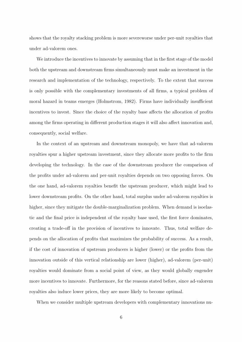
Figure 1 illustrates numerically the equilibrium prices and profits that arise from

the previous expressions. The royalty that the upstream innovator sets must trade-off

a large royalty and a small quantity resulting from double-marginalization. Following

the intuition discussed above this effect does not exist under ad-valorem royalties when

the marginal cost is 0, since in that case they effectively behave like a fixed fee. This

fact explains why the price, confirming the result stated in Proposition 1, is lower under

this royalty base, and the difference is higher for a low marginal cost. As the marginal

cost increases, the double-marginalization effect becomes more relevant under ad-valorem

royalties narrowing the gap between the resulting price and the one that emerges under

per-unit royalties.

The figure also illustrates after-investment profits under both kinds of royalties. The

result is, as expected, that upstream profits are higher under ad-valorem royalties where

the opposite is true for the downstream producer. However, an important difference

between the two kinds of royalties is that under ad valorem royalties the downstream

producer makes profits that are not monotonic in the cost. Using the intuition discussed

before about the price, when the marginal cost is low, the upstream producer can charge

a high royalty without distorting much the price. As marginal cost increases, however,

13

00.

20.

40.

60.

81

0.6

0.81

c

EquilibriumPrice(p∗)

00.

20.

40.

60.

81

0

0.1

0.2

c

UpstreamProfits(Π∗U)

00.

20.

40.

60.

81

0

0.02

0.04

0.06

c

DownstreamProfits(Π∗D)

00.

20.

40.

60.

81

0.5

0.550.6

c

UpstreamEffort(e∗U)

00.

20.

40.

60.

81

0.5

0.51

0.52

0.53

c

DownstreamEffort(e∗D)

00.

20.

40.

60.

81

0.250.3

0.35

c

SocialWelfare

Fig

ure

1:

Equilib

rium

pri

ces,

effor

tle

vels

and

soci

alw

elfa

rew

ith

per

-unit

(sol

idline)

and

ad-v

alor

em(d

ashed

line)

roya

ltie

sfo

rch

ange

sin

the

mar

ginal

costc.

Ben

chm

ark

par

amet

ers

areπU 0

=πD 0

=1.

14

this royalty must be decreased in order to keep the price low which, for some values,

compensates the producer for the higher marginal cost incurred.

Example 2 (Isoelastic Demand). Consider an isoelastic demand function D(p) = p−η

with η > 1. It is easy to show that the optimal per-unit royalties corresponds to r∗ = cη−1 .

The final price can be computed as p∗pu = c(

ηη−1

)2, where pu stands for per-unit royalties.

Profits become

Π∗U,pu =(η − 1)2η−1

η2ηc1−η,

Π∗D,pu =(η − 1)2(η−1)

η2η−1c1−η.

It is worth to notice that Π∗D,pu > Π∗U,pu. In other words, per-unit royalties allocate a

higher share of the total surplus to the downstream producer.

Under ad-valorem royalties the equilibrium royalty rate and price can be shown to be

s∗ = 1η

and p∗av = c(

ηη−1

)2, respectively.

It is interestingly to notice that the price is identical under per-unit and ad-valorem

royalties, p∗pu = p∗av. However, profits are different. In particular,

Π∗U,av =(η − 1)2(η−1)

η2η−1c1−η,

Π∗D,av =(η − 1)2η−1

η2ηc1−η.

Notice that Π∗U,av = Π∗D,pu (and obviously Π∗D,av = Π∗U,pu). In contrast to what happens

under per-unit royalties, ad-valorem royalties lead to higher profits for the upstream pro-

ducer.

The previous example shows that the isoelastic demand is a corner case of the result

in Proposition 1, one in which the prices are identical regardless of the royalty base.

This result will become handy in the rest of the paper in which we will maintain the

assumption that demand is isoelastic.

15

Assumption 1. Demand is isoelastic, D(p) = p−η, with η > 1.

This assumption on the one hand provides analytical tractability, allowing us to obtain

close form solution for most variables of the model. Furthermore, by leading to the same

price under both royalty bases it will allow us to disentangle the effects of Proposition

1 from those that will emerge once innovation incentives are considered or other market

structures, including upstream complementary innovations or downstream competition

are discussed later in the paper. It also implies that the positive effects of ad-valorem

royalties will be underestimated once we consider other demand structures.

2.2 First Stage Effort

In the first stage firms simultaneously choose their research effort. Denote the generic

expression for profits of the upstream and downstream firm resulting from the royalty

and posterior pricing stages as ΠU and ΠD, respectively.

The downstream producer chooses effort eD to maximize profits from the new product

as well as profits from the alternative use of the innovation, net of the cost of this effort.

That is, the optimal effort arises from

maxeD

eUeDΠD + eDπD0 −

1

2e2D.

In a symmetric way, the level of effort eU that maximizes profits for the upstream producer

can be obtained from

maxeU

eUeDΠU + eUπU0 −

1

2e2U .

The first order conditions for both firms lead to the following reaction functions:

eRU(eD) = eDΠU + πU0 , (1)

eRD(eU) = eUΠD + πD0 , (2)

16

and combining both reaction functions we obtain the corresponding unique equilibrium

effort decisions

e∗U =πD0 ΠU + πU01− ΠUΠD

, (3)

e∗D =πU0 ΠD + πD01− ΠUΠD

. (4)

Due to the complementarity of efforts, we observe that in equilibrium a firm’s effort

increases not only with its own profits but also with the profits of the other party. That

is, the higher the incentives a firm has to exert effort the more productive will be the

effort of the other firm. That result suggests that there might be instances in which one

firm obtains a lower proportion of the surplus and yet effort increases due to the increase

in the total surplus accrued by both firms.

The fact that under an isoelastic demand function the price is independent of whether

ad-valorem or per-unit royalties are used implies that, contingent on success, consumer

surplus is identical regardless of the kind of royalty base that the upstream developer

chooses. Furthermore, since total profits are the same in both cases, total welfare from

the production of the good, contingent on the innovation being successful, is independent

of the base used to compute the royalty.

Nevertheless, the division of the surplus might have significant implications for the

level of effort being exerted in the first place and, therefore, in the ex-ante expected

welfare. Interestingly, the next proposition states that the ranking between both kinds

of royalty structures depends only on the outside profits of both firms.

Proposition 2. If the upstream and downstream producers are monopolists and under

an isoelastic demand function, ex-ante social welfare is higher with ad-valorem royalties

if and only if πD0 ≥ πU0 .

In order to understand the previous result it is useful to start with the case in which

both firms obtain the same profits from the alternative uses of the innovation. Remem-

17

ber that the downstream producer benefits more from the production of the good under

per-unit royalties and the upstream producer benefits more under ad-valorem royalties.

Thus, it is immediate from equations (3) and (4) that under per-unit royalties a higher

proportion of the investment is carried out by the downstream producer, whereas under

ad-valorem royalties a higher proportion is carried out by the upstream developer. How-

ever, due to the symmetry in the profits that firms get in each of the cases, the total

probability of success is preserved in both cases leading to identical social welfare in both

situations.

Increases in πD0 (alternatively in πU0 ) lead to an increase in the investment of the

downstream (alternatively, the upstream) producer, as it can be appreciated from (2) (and

(1)). In equilibrium, both firms increase their investment due to the complementarity of

efforts. As we pointed out before, the two bases over which royalties can be computed

represent a trade-off, since increasing the profits and incentives to one party lowers the

equilibrium incentives of the other. The previous argument suggests that when πD0 is

high compared to πU0 , the downstream producer already has high incentives to invest.

Choosing a per-unit royalty will have little effect on downstream incentives due to the

convex cost of effort, while the lower profits it implies for the developer will discourage

upstream investment.

Using the same arguments we can conclude that the previous result would hold if,

for example, we use consumer or producer surplus as a measure of welfare rather than

total surplus. The reason is that since the price is the same in both scenarios, contingent

on success, consumer surplus and producer surplus will stay unchanged. Thus, these

measures of welfare are maximized when the probability of success is highest – given that

the first level of effort will never be attained –, which occurs under ad-valorem royalties

for πD0 ≥ πU0 .

Remark 1. Under the conditions of Proposition 2, consumer surplus and producer sur-

18

plus are higher under ad-valorem royalties if and only if πD0 ≥ πU0 .

Similar results could be obtained if we assumed that outside profits were the same for

both firms but the marginal cost of effort was different. In particular, if the cost of effort

were lower for the downstream producer so that it would naturally tend to make a higher

investment, ad-valorem royalties would be optimal, as they would spur upstream effort.

In particular, if the marginal costs of effort were C ′U(eU) = aU+eU and C ′D(eD) = aD+eD,

ad-valorem royalties would lead to higher welfare if and only if aD ≤ aU .

If Assumption 1 is relaxed, ad-valorem royalties are more likely to be optimal. Con-

sider the linear demand discussed in Example 1. Figure 1 includes the simulation of effort

decisions and ex-ante social welfare assuming that outside profits are identical. Although

per-unit royalties spur the investment of the downstream producer and ad-valorem roy-

alties spur the investment of the upstream developer the two effects are not of the same

magnitude. The probability of success is higher under ad-valorem royalties since the

double-marginalization effect is smaller and, thus, total profits are higher in this case.

The combination of the higher incentives to innovate together with a lower price makes

social welfare higher under ad-valorem royalties. Of course, as in the isoelastic case,

the results could be overturned by choosing πU0 sufficiently higher than πD0 . Numerical

simulations suggest, however, that this difference might need to be substantial for such

a change to occur.

3 Multiple Upstream Developers

In this section we extend the previous framework to consider the possibility that there

might be several upstream firms that contribute different pieces of the technologies neces-

sary for the downstream product to be successful. In particular, we assume that there are

NU > 1 components researched by NU different developers. Component i is researched

by upstream firm i, for i = 1, ..., , NU . We assume that these components are symmetric

19

so that the cost for developer i of exerting effort eiU is C(eiU) = 12(eiU)2. Similarly, the

probability of success is symmetric and equal to

E =

(NU∑i=1

(eiU)α

) 1α

eD,

where α ∈ [0, 1] measures the degree of independence of the different innovations. When

α is high the effect of effort of firm i on the productivity of the effort of firm j is small.

As α decreases innovations become more complementary. The existence of a Standard

Setting Organization (SSO) that aims to coordinate the firms that provide technologies

for a product would be consistent with a low value of α.7 As before, we assume that the

alternative uses of each innovation carried out by an upstream producer lead to profits

πU0 > 0.

In the first stage firms simultaneously choose their research effort. The unique down-

stream producer chooses eD to maximize

maxeD

(NU∑i=1

(eiU)α

) 1α

eDΠD + eDπD0 −

1

2e2D.

Upstream developer i chooses eiU to maximize,

maxeiU

(NU∑i=1

(eiU)α

) 1α

eDΠU + eiUπU0 −

1

2(eiU)2.

In a symmetric equilibrium we have a generalization of equations (3) and (4) to NU > 1,

implying that

e∗D =N

1/αU ΠDπ

U0 + πD0

1−N2−αα

U ΠUΠD

,

e∗U =N

1−αα

U ΠUπD0 + πU0

1−N2−αα

U ΠUΠD

.

The same kind of complementarity discussed in the case of one upstream developer op-

erates here between different developers. Keeping profits constant, increases in NU raise

7For simplicity we assume that all components are required for the final product, as in the case ofStandard Essential Patents (SEPs). In section 5.2 we show that results still hold when we relax thisassumption.

20

the probability of success of the innovation and thus the incentives of all parties to invest.

Of course, profits in the final stages of the game will change as NU increases, affecting

this result. We now analyze the direction of these changes and, in particular, how the

profits of the upstream developers and the downstream producers are shaped under the

different bases for the royalty rate as NU increases.

3.1 Per-Unit Royalties

Under per-unit royalties, the total royalty rate that the downstream producer faces is

R ≡∑NU

i ri. Thus, the optimal downstream price is identical to the one in the case in

which NU = 1 obtained before but applied to the total rate, p∗(R) = ηη−1(c+R).

Anticipating that price, all upstream developers simultaneously choose their royalty

rate ri, for i = 1, ..., NU to maximize profits. For developer i this maximization implies

maxri

ri (p∗(R))−η .

Differentiating with respect to ri and focusing on a symmetric equilibrium, in which

ri = r∗ for all i, we have that

r∗ =c

η −NU

and p∗pu =η2

(η − 1)(η −NU)c,

which are defined only if η > NU . We see that the higher the number of upstream

producers the higher the price in the final market and, thus, the larger the final market

distortions. This result is a standard application of the idea of Cournot complements.

Upstream developers only take into account the effect of their royalty on their own profits

but not the fact that it reduces the quantity that is also the base of the revenues of all

other upstream developers.

Profits can be computed as

Π∗U,pu =(η −NU)η−1(η − 1)η

η2ηc1−η,

Π∗D,pu =(η −NU)η−1(η − 1)η−1

η2η−1c1−η,

21

which are decreasing in NU due to the previous effect.

3.2 Ad-Valorem Royalties

Under ad-valorem royalties the total royalty rate is again S ≡∑NU

i si. Using the expres-

sion for the royalty in the case of NU = 1 applied to the total royalty rate we have that

pM(S) = η(1−S)(η−1)c.

Upstream developer i chooses si in the first stage to maximize

maxsi

si (p∗(S))1−η .

Differentiating with respect to si and focusing on a symmetric equilibrium, in which

si = s∗ for all i, we have that

s∗ =1

η +NU − 1and p∗av =

η(η +NU − 1)

(η − 1)2c,

where as before the price is increasing in NU . Profits can be computed as

Π∗U,av =(η − 1)2η−2

ηη−1(η +NU − 1)ηc1−η,

Π∗D,av =(η − 1)2η−1

ηη(η +NU − 1)ηc1−η.

3.3 Comparison

We start by analyzing the pricing stage, once investment has been carried out and all

components of the innovation has been successfully developed, both upstream and down-

stream.

Proposition 3. Suppose that innovation efforts have been successful. Under ad-valorem

royalties the final price is lower, p∗av ≤ p∗pu. Furthermore, upstream producers’ profits are

higher under ad-valorem royalties whereas the downstream producer’s profits are higher

under per-unit royalties.

22

0.5

0.6

0.7

0.8

0.9

10.

5

0.550.6

c

UpstreamEffort(e∗U)

0.5

0.6

0.7

0.8

0.9

1

0.6

0.7

c

DownstreamEffort(e∗D)

0.5

0.6

0.7

0.8

0.9

1

0.4

0.5

0.6

c

TotalWelfare

12

34

0.5

0.6

0.7

NU

UpstreamEffort(e∗U)

12

34

0.5

0.6

0.7

0.8

NU

DownstreamEffort(e∗D)

12

34

0.5

0.6

0.7

0.8

NU

TotalWelfare

Fig

ure

2:

Eff

ort

by

upst

ream

dev

elop

ers,

the

dow

nst

ream

pro

duce

r,an

dto

tal

wel

fare

under

the

use

ofp

er-u

nit

(sol

idline)

and

ad-v

alor

em(d

ashed

line)

roya

ltie

sfo

rch

ange

sin

the

mar

ginal

costc

(ab

ove)

and

the

num

ber

ofupst

ream

dev

elop

ers,NU

(bel

ow).

The

bas

elin

epar

amet

erva

lues

areπD 0

=πU 0

=0.

5,α

=0.

7,NU

=2,η

=4,

andc

=0.

5

23

0.5

0.6

0.7

0.8

0.9

1

0.6

0.7

α

UpstreamEffort(e∗U)

0.5

0.6

0.7

0.8

0.9

1

0.6

0.81

α

DownstreamEffort(e∗D)

0.5

0.6

0.7

0.8

0.9

1

0.5

0.550.6

0.65

α

TotalWelfare

23

45

0.5

0.6

0.7

η

UpstreamEffort(e∗U)

23

45

0.6

0.8

η

DownstreamEffort(e∗D)

23

45

0.4

0.6

0.8

η

TotalWelfare

Fig

ure

3:

Eff

ort

by

upst

ream

dev

elop

ers,

the

dow

nst

ream

pro

duce

r,an

dto

tal

wel

fare

under

the

use

ofp

er-u

nit

(sol

idline)

and

ad-v

alor

em(d

ashed

line)

roya

ltie

sfo

rch

ange

sin

the

subst

itubilit

yb

etw

een

innov

atio

nsα

(ab

ove)

,an

dth

eel

asti

city

ofth

edem

and,

η(b

elow

).T

he

bas

elin

epar

amet

erva

lues

areπD 0

=πU 0

=0.

5,α

=0.

7,NU

=2,η

=4,

andc

=0.

5

24

Some of the results obtained in the case of one upstream developer are preserved

in this case. It still true that ad-valorem royalties tend to favor upstream developers,

compared to the downstream producer, whereas the opposite is true for per-unit royalties.

An important difference, however, is that ad-valorem royalties lead to lower downstream

prices. Thus, ex-post consumer surplus is lower under per-unit royalties.

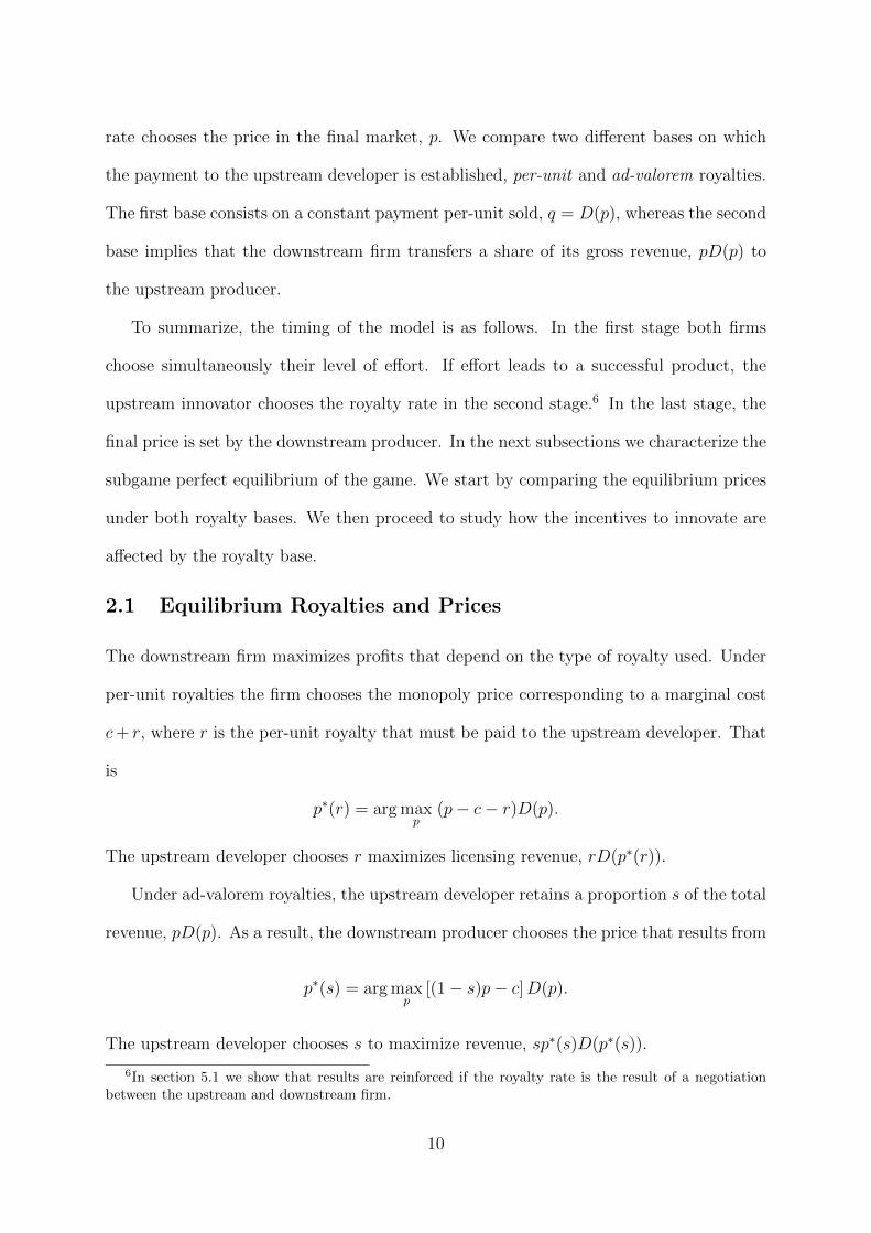
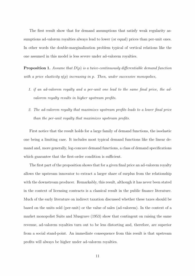
In order to understand the ex-ante incentives, however, we need to rely on numerical

analysis. In Figures 2 and 3 we provide an example of the effects of the different parame-

ters of the model over the equilibrium decisions in the first stage of the model, upstream

and downstream effort, together with social welfare.

The results indicate that ad-valorem royalties translate into higher investment by up-

stream developers. This effect is particularly important for low values of c and α. In the

case of the former, as in the one upstream innovator case, the result stems from the fact

that the double-marginalization effect under ad-valorem royalties is small when c is low,

implying a large optimal royalty s∗ and large upstream profits which spur investment. For

the latter, notice that low values of α imply that the investment of different upstream pro-

ducers are more complementary. As a result, the higher profits that ad-valorem royalties

imply are reinforced by the increased investment of other innovators.

In the case of the downstream producer the equilibrium effect on investment is the

combination of two forces. On the one hand, ad-valorem royalties lead to lower down-

stream profits contingent on success, as illustrated in Proposition 3, which feed back into

lower incentives to invest. On the other hand, as mentioned in the previous paragraph,

upstream innovators invest more and, under the complementarity of investments assump-

tion, the marginal productivity of downstream investment raises. The results indicate

that the second force typically dominates and downstream investment also raises under

ad-valorem royalties. The only exception corresponds to the case in which NU < 2. From

the previous section we know that under ad-valorem royalties when there is only one

25

upstream developer downstream profits are lower and so are the incentives to innovate.

Total welfare is generally higher under ad-valorem royalties. This result arises due to

two reasons. First, ad-valorem royalties lead to lower final prices, favoring consumers.

Second, they typically generate an increase in total investment and in the resulting prob-

ability of product success. The difference in total surplus is particularly large when we

consider more complementary upstream innovations.

4 Downstream Competition

We now analyze the opposite case to the one discussed in the previous section. We in-

troduce downstream competition while assuming that, as in the benchmark model, there

is a unique upstream developer. Consistent with the rest of the paper we assume that

downstream producer i exerts effort eiD at a cost C(eiD) =(eiD)2

2. That effort in combi-

nation with upstream investment, leads to a probability eUeiD of technological success of

the product of firm i.

Of course, when there are potentially multiple downstream producers, technological

success does not immediately translate into market success. It depends on the techno-

logical success or failure of the competitors. In order to simplify the analysis we assume

that all downstream firms, if successful, sell an identical product and compete in prices

so that profits are 0 if more than one firm succeeds. Furthermore, in order to illustrate

our results we focus our discussion on the case in which there are just two downstream

producers, ND = 2.

In the first stage downstream producer i = 1, 2 chooses effort to maximize

maxeiD

eUeiD(1− ejD)ΠD + eiDπ

D0 −

(eiD)2

2,

where j 6= i. The previous expression indicates that downstream producer i only obtains

profits from the production of the good when that firm and the upstream producer

26

succeed while the downstream competitor fails. In that case, downstream profits, ΠD,

are identical to those obtained in the benchmark case. Otherwise, profits arise only from

the alternative uses of the innovation.

The upstream producer chooses effort to maximize

maxeU

eUe1De

2DΠU(2) + eU

[e1D(1− e2D) + (1− e1D)e2D

]ΠU(1) + eUπ

U0 −

e2U2.

The profits from royalties in the last stage of the game depend on the number of final good

producers that end up competing in the market. When only one producer succeeds profits

become ΠU(1), identical to the profits in the benchmark model. Alternatively, when both

downstream producers succeed upstream equilibrium profits, ΠU(2), have a very simple

expression arising from the following logic. Downstream Bertrand competition eliminates

the double marginalization and, consequently, the price in the final market corresponds

to the perceived marginal cost of each downstream producer (c + r and c1−s under per-

unit and ad-valorem royalties, respectively). For this reason, the upstream producer

will find optimal to choose a royalty rate that induces the monopoly price downstream,

pM = ηη−1c. In this way, the upstream monopolist will obtain monopoly profits regardless

of the royalty scheme used. These profits can be computed as

Π∗U,pu(2) = Π∗U,av(2) = πM =(η − 1)η−1

ηηc1−η.

Incidentally, it is important to point out that it is only in this context of ex-post perfect

competition that per-unit and ad-valorem royalties (and consequently the apportionment

and the entire market value rule) are equivalent.

The previous maximizations characterize the symmetric equilibrium of the first stage

– that is when all downstream producers choose the same investment level –, through the

27

intersection of the reaction functions HU(eD) and HD(eU)

e∗U = HU(e∗D) = (e∗D)2 πM + 2(1− e∗D)e∗DΠU + πU0 ,

e∗D = HD(e∗U) =e∗UΠD + πD01 + e∗UΠD

.

for the upstream and downstream producers, respectively. It is easy to see that increases

in eD always increase the investment incentives of the upstream producer. This result

is due to the fact that increases in eD make the downstream duopoly case more likely

and, thus, the returns from the investment upstream raise. In contrast, the effects of

eU on downstream investment are the result of two opposing forces. On the one hand,

increases in eU make technological success more likely and, due to the complementarity,

the incentives to invest downstream increase. On the other hand, each downstream pro-

ducer anticipates that the competitor might have more incentives to invest and monopoly

profits will be less likely to arise. This second effect reduces the incentives to invest in

the first place and it is more important the larger are the exogenous reasons to invest,

πD0 .

The effects of ΠU and ΠD on investment can be described along the same lines.

Whereas the direct effect of increases in ΠU on e∗U is positive, increases in ΠD generate

two opposing effects for the reasons discussed above.

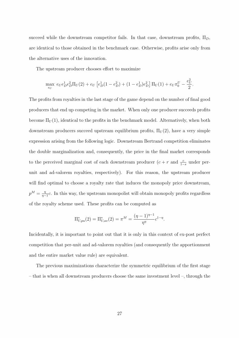
As in the case of multiple upstream innovators, it is difficult to have analytical results

and, for this reason, we again rely on numerical simulations. Figure 4 shows how the

effort of the upstream developer and downstream producers change when marginal cost

and the elasticity of the demand vary under both per-unit and ad-valorem royalties.

The results indicate that, as expected and consistent with the rest of the paper,

ad-valorem royalties in general spur the investment of the upstream developer whereas

per-unit royalties provide more incentives for the downstream firms to invest. These

differences become more significant when demand elasticity is low. Regarding costs, we

28

0.2

0.4

0.6

0.8

1

0.51

c

UpstreamEffort(e∗U)

0.2

0.4

0.6

0.8

1

0.2

0.4

0.6

c

DownstreamEffort(e∗D)

0.2

0.4

0.6

0.8

1

024

c

TotalWelfare

22.

53

3.5

4

0.14

0.16

0.180.2

η

UpstreamEffort(e∗U)

22.

53

3.5

4

0.12

0.13

0.14

0.15

η

DownstreamEffort(e∗D)

22.

53

3.5

40.

04

0.05

0.06

0.07

η

TotalWelfare

Fig

ure

4:

Eff

ort

by

upst

ream

dev

elop

ers,

two

dow

nst

ream

pro

duce

rs,

and

tota

lw

elfa

reunder

the

use

ofp

er-u

nit

(sol

idline)

and

ad-v

alor

em(d

ashed

line)

roya

ltie

sfo

rch

ange

sin

the

mar

ginal

costc

and

the

elas

tici

tyof

dem

and,η.

Ben

chm

ark

par

amet

erva

lues

areη

=2,c

=0.

5,an

dπU 0

=πD 0

=0.

1.

29

observe that when the marginal cost is small ad-valorem royalties do not lead to signifi-

cantly higher effort upstream while at the same time downstream effort is reduced. This

result arises from the fact that when the marginal cost is low double marginalization is

small under ad-valorem royalties, leading the upstream developer to charge a high roy-

alty, which once anticipated discourages downstream investment. The complementarity

between investments reduces the upstream incentives to innovate. The combination of

both forces leads to lower welfare under ad-valorem royalties, due to the lower probability

of success it entails.

When marginal costs increase, however, upstream effort becomes significantly higher

under ad-valorem royalties which compensates the lower investment by downstream pro-

ducers due to their lower expected profits contingent on success. From the point of view

of social welfare, ad-valorem royalties lead to higher total surplus only when marginal

cost is large, although the magnitude of the difference in either direction is difficult to

appreciate in the simulation. Thus, the implications of downstream competition are likely

to be second order when compared to the impact of introducing other upstream producers

or of considering other demand functions. In both cases, ad-valorem royalties are likely

to be preferred as we saw in section 3 for the former and we will see in the next section

for the latter.

5 Robustness Analysis

In this section we analyze how the results are affected by changes in some of our main-

tained assumptions. First, we study the case in which the royalty is not set by the

upstream developer but it is the result of the negotiation between both parties. Second,

we relax the perfect complementarity between innovations assumed in section 3. In all

cases, the main message of the paper is unchanged.

30

5.1 Bargained Royalty Rate

We have assumed throughout the paper that the royalty rate (either per-unit or ad-

valorem) was the result of a take-it-or-leave-it offer made by the upstream producer.

Having accepted the offer, the downstream producer decided the final price. We now

generalize the model and assume that the royalty rate is the result of a bargaining process

between the upstream and the downstream producer. The final price, however, is still

independently chosen by the downstream firm.

In particular, we assume that the equilibrium royalty emerges as the result of Nash

bargaining in which the bargaining power of the upstream and downstream firms are γ

and 1− γ, respectively, for γ ∈ [0, 1]. Using the maintained assumption in the rest of the

paper that the contribution of the upstream and downstream parties is essential for the

product to be marketable – and that we will relax in section 5.2 –, the outside option in

the negotiation of each of the parties is set to 0.

Starting with per unit royalties, given a royalty r, the final price comes from section

2, p∗(r) = (c + r) ηη−1 . Profits correspond to ΠU(r) = r(p∗(r))−η and ΠD(r) = (p∗(r) −

(c+ r))p∗(r)−η. Hence, the equilibrium royalty results from

r∗ = arg maxr

ΠU(r)γΠD(r)1−γ,

or r∗ = γcη−1 . The equilibrium price becomes p∗pu = cη(η+γ−1)

(η−1)2 . This price, of course, is

increasing in γ, as the problem of double-marginalization becomes more important the

higher the bargaining power allocated upstream.

Under ad-valorem royalties, given a royalty s, the final price is p∗(s) = cη(1−s)(η−1) .

Profits can be written as ΠU(s) = s(p∗(s))1−η and ΠD(r) = ((1−s)p∗(s)−c)p∗(s)−η. The

equilibrium royalty results from

s∗ = arg maxs

ΠU(s)γΠD(s)1−γ,

31

0 0.2 0.4 0.6 0.8 1

0.6

0.7

0.8

0.9

1

1.1

1.2

γ

Equilib

rium

Pri

ce(p∗ )

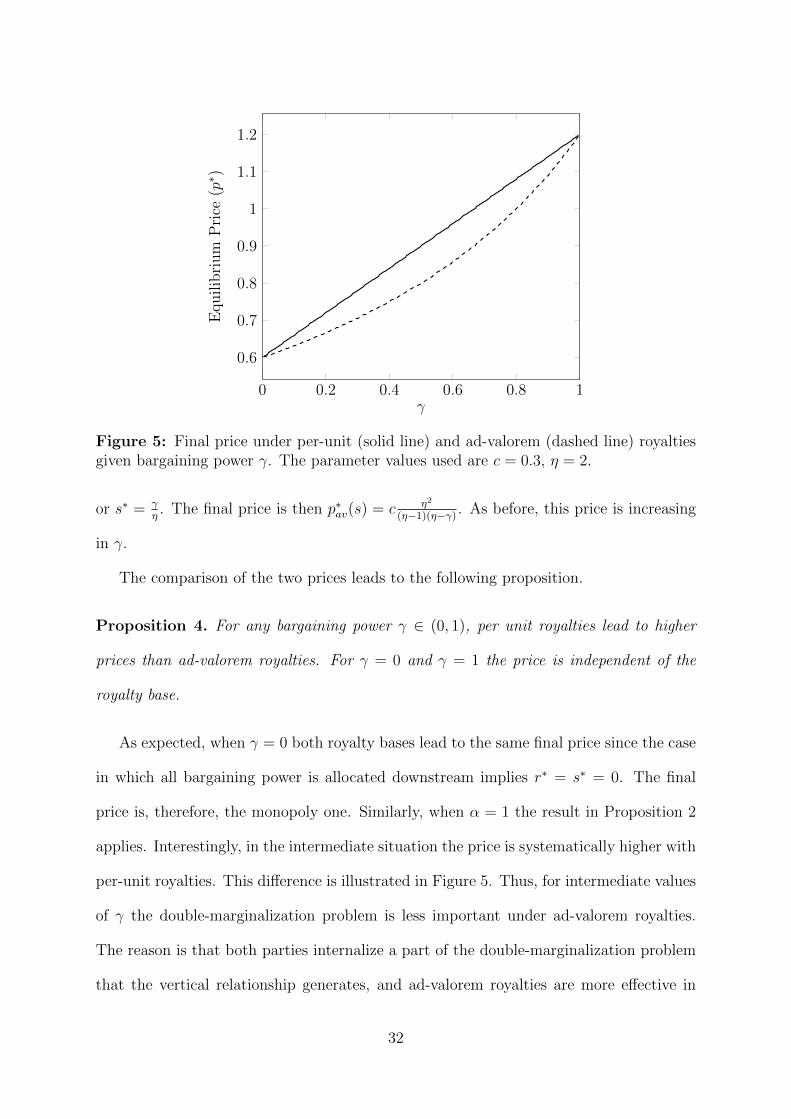
Figure 5: Final price under per-unit (solid line) and ad-valorem (dashed line) royaltiesgiven bargaining power γ. The parameter values used are c = 0.3, η = 2.

or s∗ = γη. The final price is then p∗av(s) = c η2

(η−1)(η−γ) . As before, this price is increasing

in γ.

The comparison of the two prices leads to the following proposition.

Proposition 4. For any bargaining power γ ∈ (0, 1), per unit royalties lead to higher

prices than ad-valorem royalties. For γ = 0 and γ = 1 the price is independent of the

royalty base.

As expected, when γ = 0 both royalty bases lead to the same final price since the case

in which all bargaining power is allocated downstream implies r∗ = s∗ = 0. The final

price is, therefore, the monopoly one. Similarly, when α = 1 the result in Proposition 2

applies. Interestingly, in the intermediate situation the price is systematically higher with

per-unit royalties. This difference is illustrated in Figure 5. Thus, for intermediate values

of γ the double-marginalization problem is less important under ad-valorem royalties.

The reason is that both parties internalize a part of the double-marginalization problem

that the vertical relationship generates, and ad-valorem royalties are more effective in

32

aligning the incentives, as they take into account the effect on the price.

5.2 Other Upstream Complementarities

The model in section 3 assumes that several upstream producers contribute complemen-

tary technologies. These technologies are perfectly complementary from the downstream

producer point of view in the sense that all of them are required to be licensed for the

product to be marketed. The technologies are less complementary in the development

stage, and the higher is α the more independent these technologies become in that stage.

In this section we study the implications of relaxing the previous assumption and assume

that from the point of view of the downstream users technologies might not be perfectly

complementary and, thus, not all of them might be required for the production of the

good.

In particular, we assume that the marginal cost of the downstream producer is de-

creasing in the number of innovations licensed and takes the form C(N) = cN−β where

N ≤ NU is the number of technologies licensed and β > 0. By varying the value of β

we can spawn different levels of downstream complementarity between innovations. A

value of β close to 0 makes the marginal cost independent of the number of innovations

licensed, which implies that they become close substitutes. Larger values of β increase

the marginal valuation of additional innovations. When β > 1 technologies essentially

become complements, since the cost reduction is increasing in the number of technologies

licensed.

5.2.1 Per-Unit Royalties

The monopoly price when the downstream producer has licensed N innovations corre-

sponds to p∗(R,N) = ηη−1(cN−β + R), where R is the sum of all the royalties paid.

33

Downstream producer profits can be written as

ΠD(R,N) =(η − 1)η−1

ηη(cN−β +R)1−η.

Notice that in equilibrium all innovations must be licensed. Otherwise, left-out up-

stream producers would decrease the royalty rate in order to have their innovation li-

censed. In particular, let’s consider the royalty rate of innovator i, ri, when all other

innovators have chosen a royalty r. The licensing decision can be obtained from the

expression

maxri

ri(pM(R,NU))−η

s.t. ΠD(R,NU) ≥ ΠD (R− ri, NU − 1) ,

whereR ≡ (NU−1)r+ri is the total royalty. The constraint indicates that the downstream

producer will license the innovation if it leads to higher profits than if it licenses only

NU − 1 technologies. This constraint can be rewritten as

ri ≤ r ≡ c[(NU − 1)−β −N−βU

]. (5)

If the constraint is not binding the optimal royalty is identical to the one obtained in

section 3. Thus, the royalties resulting from a symmetric equilibrium can be written as

r∗ = min

{cN−βUη −NU

, r

}.

5.2.2 Ad-Valorem Royalties

The monopoly price under ad-valorem royalties when N innovations are licensed can be

written as p∗(S,N) = η(1−S)(η−1)cN

−β, where S is the total royalty paid. Replacing in the

profit function of the downstream producer we obtain

ΠD(S,N) =(η − 1)η−1

ηη

(cN−β

)(1−η)(1− S)−η

.

34

As in the previous case, all technologies will be licensed in equilibrium. We focus on

a symmetric equilibrium, in which the optimal decision of innovator i takes as given the

royalty of all other innovators, s. In that case, si results from the maximization

maxsi

si (p∗(S,N))1−η

s.t. ΠD(S,NU) ≥ ΠD ((NU − 1)s,NU − 1) .

where S = (NU − 1)s + si is the total royalty. The previous constraint, which accounts

for the fact that the downstream producer must prefer to license technology i to using

only the other ones, is satisfied if

si ≤ s ≡ N−β(η−1)/ηU − (NU − 1)−β(η−1)/η

(NU − 1)N−β(η−1)/ηU −NU(NU − 1)−β(η−1)/η

. (6)

The optimal royalty will correspond to the one that maximizes profits in section 3 when

it is lower than the previous constraint or s otherwise. That is,

s∗ = min

{1

η +NU − 1, s

}.

5.2.3 Comparison

Figure 6 provides a numerical example of the model for different values of β both under

per-unit and ad-valorem royalties. Regardless of the case, we can observe that the optimal

royalty function is composed of two segments. When β is low innovations are close

substitutes. For this reason, the willingness to pay of downstream producers is low, forcing

developers to ask for a low royalty that approaches 0 as innovations become closer to

perfect substitutes. The functions r and s in equations (5) and (6) describe that region of

values of β. When substitubility is low (or technologies become complements) the optimal

royalty takes an interior value in the maximization, making the expression identical to

the one obtained in the main part of the paper. Ad-valorem royalties become then

independent of costs. Per-unit royalties are decreasing in β, since greater complementarity

35

0 0.5 1 1.5 20

0.05

0.1

0.15

0.2

β

Equilib

rium

Roy

alty

0 0.5 1 1.5 2

0.4

0.6

0.8

β

Fin

alP

rice

(p∗ )

0 0.5 1 1.5 2

0

5

10

β

Upst

ream

Pro

fits

(Π∗ U

)

0 0.5 1 1.5 2

0

5

10

15

β

Dow

nst

ream

Pro

fits

(Π∗ D

)

Figure 6: Equilibrium royalties, prices, and profits contingent on success of the innova-tion with per-unit (solid line) and ad-valorem (dashed line) royalties as a function of β.The remaining parameters are chosen as follows: η = 4, NU = 2, and c = 0.5.

decreases costs, providing incentives for developers to charge lower royalties which benefit

them through the increase in quantity produced.

The figure also shows that prices are higher under per-unit royalties, and this difference

exists regardless of the level of complementarity between their innovations. This result

reinforces Proposition 3 that showed this result for perfect complementarity. The shape

of equilibrium prices responds to the evolution of royalty rates and the decrease in costs

that higher values of β entails. Higher royalty rates or higher costs are passed through

higher prices.

Finally, profits display the same properties as those in our benchmark case. Under ad-

36

valorem royalties upstream profits are higher whereas downstream profits are lower. These

differences exist for all values of β but they are particularly significant as innovations

become more complementary.

6 Concluding Remarks

We have shown that royalties based on the value of sales – i.e. royalties where the scope of

the royalty base is determined by the entire market value rule – yield superior outcomes

from both consumer welfare and total welfare standpoints than per-unit royalty rates – i.e.

royalties where the scope of the royalty base is determined by reference to the value of the

components of the infringing product that are covered by the patented technology. Only

under very specific and rather implausible circumstances, such as perfect competition

among implementers and end products incorporating technologies from a single licensor,

the opposite may be true.

Our models abstract from implementation issues. When those are taken into account,

the welfare superiority of the entire market value rule, and hence of the ad-valorem royal-

ties, is only reinforced. In our analysis, ad-valorem royalties are better from the consumer

welfare and total welfare perspectives for two reasons. First, the entire market value rule

mitigates the double marginalization problem that naturally arises in technology markets

characterized by market power at the licensing and manufacturing levels of the vertical

chain. This is because licensors internalize the impact on the prices of the end products of

an increase in their royalty rate to a greater extent when the royalty base is given by the

entire market value of the product. Second, investments by both technology companies

and implementers are greater under the entire market value rule because overall industry

profits, and hence the incentives to innovate, are greater when the double marginaliza-

tion problem is less severe. This effect is stronger, and therefore the entire market value

rule is even more attractive, when there are multiple innovators licensing complementary

37

technologies. Because ad-valorem royalties shift profits upstream, they compensate the

tendency to underinvest by owners of complementary technologies.

Our findings apply to technology markets where patent owners face limited competi-

tion from substitute technologies. In fact, our models focus on the extreme case where

each patent owner enjoys monopoly power and to the extent that there are multiple

patent holders, each of them owns a set of patents that is complementary to the patents

of the others. As a result, our models can be used to develop normative implications in

the context of standard essential patents or SEPs. Our findings suggest that it would be

wrong to mandate per-unit royalties for SEPs and that, to the extent that policy-makers

are concerned about the possibility of patent hold up and royalty stacking, they should

advocate in favor of the entire market value rule, as that is likely to result in greater

consumer and social welfare.

38

References

Bousquet, Alain, Helmuth Cremer, Marc Ivaldi and Michel Wolkowicz,

“Risk sharing in licensing,” International Journal of Industrial Organization, Septem-

ber 1998, 16 (5), pp. 535–554.

Colombo, Stefano and Luigi Filippini, “Patent licensing with Bertrand competi-

tors,” DISCE - Quaderni dell’Istituto di Teoria Economica e Metodi Quantitativi

itemq1262, Universit Cattolica del Sacro Cuore, Dipartimenti e Istituti di Scienze

Economiche (DISCE), April 2012, URL http://ideas.repec.org/p/ctc/serie6/

itemq1262.html.

Geradin, Damien and Anne Layne-Farrar, “Patent Value Apportionment Rules

for Complex, Multi-Patent Products,” Santa Clara Computer & High Technology Law

Journal , 2011, 4 (27), pp. 763–792.

Gilbert, Richard J. and Michael L. Katz, “Efficient Division of Profits from

Complementary Innovations,” International Journal of Industrial Organization, July

2011, 29 (4), pp. 443–454.

Holmstrom, Bengt, “Moral Hazard in Teams,” Bell Journal of Economics , Autumn

1982, 13 (2), pp. 324–340.

Love, Brian J., “Patent Overcompensation and the Entire Market Value Rule,” Stan-

ford Law Review , 2007, 60 (1), pp. 263–294.

Salop, Steven C. and David T. Scheffman, “Raising Rivals’ Costs,” The American

Economic Review , 1983, 73 (2), pp. pp. 267–271.

San Martın, Marta and Ana I. Saracho, “Royalty licensing,” Economics Letters ,

May 2010, 107 (2), pp. 284–287.

Sherry, Edward F. and David J. Teece, “Some Economic Aspects of Intellectual

Property Damages,” PLI/PAT , 1999, 572 , pp. 399–403.

Suits, D. B. and R. A. Musgrave, “Ad Valorem and Unit Taxes Compared,” The

Quarterly Journal of Economics , 1953, 67 (4), pp. 598–604.

39

A Proofs

Lemma A.1. A twice continuously differentiable profit function Π(p) = (p − c)D(p) is

quasiconcave if the elasticity of the demand η(p) = −D′(p)pD(p)

is increasing in p.

Proof of Lemma A.1: A single variable function Π(p) is quasiconcave if (i) it is

either always increasing or always decreasing in p or (ii) if there exists a p∗ such that

Π(p) is increasing for p < p∗ and decreasing for p > p∗.

Let’s assume, towards a contradiction that neither of the two previous conditions

is true. In that case, at least one of the solutions to the first order condition must

characterize a minimum. We now show that this cannot occur and there is at most one

solution characterized by the first order condition which determine a maximum.

The Lerner indexp∗ − cp∗

=1

η(p∗)

shows that there can be at most one solution, since the left-hand side is always increasing

while the right hand side is always decreasing, when η(p) is increasing in p.

We now show that this unique critical value p∗ always defines a maximum. In order

to do that, notice that

∂η

∂p= −D

′(p)D(p) + pD′′(p)D(p)−D′(p)2

D2(p).

This expression is positive if and only if

D′′(p) ≤ D′(p)2

D(p)− D′(p)

p,

We can now compute

Π′′(p∗) = D′′(p∗)(p∗ − c) + 2D′(p∗) < D′(p∗)

(1− 1

η(p∗)

)= D′(p∗)

p∗ − cp∗

< 0,

where first inequality comes from the upper bound on D′′(p) originating from the previous

expression. Thus, the profit function is quasi-concave.

Lemma A.2. Assume that D(p) is a twice-continuously differentiable demand function

with a price elasticity η(p) increasing in the price. Then, under per-unit royalties the

optimal price has an upper bound

p∗pu ≤(c+ r∗)2

c.

40

Proof of Lemma A.2: Using Lerner’s rule we have that under per-unit royalties

the optimal price is determined as(1− 1

η(p∗pu)

)p∗pu = c+ r, (A.1)

where we have made explicit the dependency of the demand elasticity η on p. Using the

Implicit Function Theorem we have that

∂p∗pu∂r

=1(

1− 1η(p)

)+ p

η(p)2η′(p)

> 0. (A.2)

In the first stage the upstream developer chooses the royalty to maximize rD(p∗pu(r)),

resulting in a first order condition

D(p∗pu(r∗)) + r∗D′(p∗pu(r

∗))∂p∗pu∂r

= 0.

Solving for r∗ and after replacing (A.2) we have that

r∗ = −D(p∗pu(r

∗))

D′(p∗pu(r∗))

∂p∗pu∂r

=p∗pu

(1− 1

η(p∗pu)

)+

(p∗pu)2

η(p∗pu)2η′(p∗pu)

η(p∗pu).

Substituting r∗ in (A.1), the first-order condition for the downstream producer, and

rearranging terms we have(1− 1

η(p∗pu)

)2

p∗pu = c+(p∗pu)

2

η(p∗pu)3η′(p∗pu).

We can now replace the left hand side expression by (c+r)2

cp∗puand rearrange terms to obtain

p∗pu =(c+ r∗)2

c+(p∗pu)

2

η(p∗pu)3η′(p∗pu)

≤ (c+ r∗)2

c

where the last inequality arises from η′(p) ≥ 0.

Proof of Proposition 1: For the first part, take a per-unit royalty r. The profit

maximizing price for the downstream producer satisfies(1− 1

η

)D(p∗pu) = c+ r (A.3)

whereas with ad-valorem royalties the same price could be reached with a royalty s such

that

(1− s)(

1− 1

η

)D(p∗av) = c. (A.4)

41

Notice that to simplify notation we have dropped the argument in the demand elasticity

η. From Lemma A.1 these first order conditions are necessary and sufficient.

It is immediate that the two royalties lead to the same price if and only if

r =s

1− sc.

Upstream profits under per-unit royalties are

ΠU,pu(r) = rD(p∗) = sc

1− sD(p∗) < sp∗D(p∗) = ΠU,pu(s),

where the last inequality comes from the fact that (1− s)p∗ > c

For the second part, take the optimal per-unit royalty r∗ and the equilibrium price

p∗pu = p∗. As shown before, this same price could be induced under an ad-valorem royalty

s = rc+r

. Given the concavity of the profits of the upstream producer it is enough to show

that the derivative of the profits of the upstream producer evaluated at s is positive. In

particular,∂ΠU,av

∂s(s) = p∗D(p∗) + s [pD′(p∗) +D(p∗)]

∂p∗

∂s.

Using the Implicit Function Theorem on (A.3) and (A.4) and using the fact that under

s the equilibrium price is the same we have that

∂p∗av∂s

=

(1− 1

η

)D(p∗)

1− s∂p∗

∂r=c+ r∗

1− s∂p∗

∂r.

Replacing in the previous first order condition together with the expression for s and the

fact that p∗D′(p∗) +D(p∗) = (c+ r)D′(p∗) from the optimality of p∗ we have that

∂ΠU,av

∂s(s) = p∗avD(p∗av) +

r∗(c+ r∗)2

cD′(p∗)

∂p∗

∂r.

Finally, notice that the first order condition that pins down r∗ implies that D′(p∗)∂p∗

∂r=

D(p∗)r∗

and replacing we have that

∂ΠU,av

∂s(s) =

[p∗av −

(c+ r∗)2

c

]D(p∗av) < 0

where the last inequality comes from Lemma A.2.

Proof of Proposition 2: Given that prices in both cases are identical, pMav = pMpu =

pM consumer surplus contingent on success is constant and can be written as

CS ≡∫ ∞pM

p−ηdp.

42

Consider a given level of profits for the upstream developer and downstream producer

ΠU and ΠD, respectively. The social welfare function can be written as

W = e∗Ue∗D(CS + ΠU + ΠD) + e∗Uπ

U0 + e∗Dπ

D0 −

(e∗u)2

2− (eD)2

2,

where e∗U and e∗D can be obtained from (3) and (4). Given that Π∗U,pu + Π∗D,pu = Π∗U,av +

Π∗D,av it is immediate that CS + ΠU + ΠD is identical in both cases. Furthermore,

equilibrium effort levels are the same if πU0 = πD0 , implying that the expected total

surplus is the same under both kinds of royalties.

In order to show the result it is enough to show that ∂W∂πUo

is higher under per-unit

royalties (and by symmetry ∂W∂πDo

is lower under ad-valorem royalties). This derivative can

be computed as

∂W

∂πU0=πD0 (ΠUΠD + 1) + 2πU0 ΠD

(1− ΠUΠD)2CS +

πD0 (ΠU + ΠD) + ΠU0 (π2

D + 1)

(1− ΠUΠD)2.

It is easy to observe that since ΠU + ΠD and ΠUΠD are constant under both kinds of

royalty rates, the derivative will be higher in the case for which ΠD is biggest. This

corresponds to per-unit royalties.

Proof of Proposition 3: The ordering of the prices is immediate from their expres-

sions. The inequality is strict when NU > 1.

Regarding profits, notice that

Π∗D,puΠ∗U,pu

=η

η − 1=

Π∗U,avΠ∗D,av

,

where ηη−1 > 1 proving the second part of the result.

Proof of Proposition 4: Immediate from the comparison of both prices.

43