The Optimal Degree of Centralization

Charles Z. Zheng∗

April 10, 2016

Abstract

This paper considers a normative foundation of government based on a Hobbesian

anarchy where one region may pillage the other. A center that takes enough power

from the regions and helps the victim to fight the aggressor can deter warfare thereby

incentivizing productive efforts of the regions, but with less power the regions become

less productive. This paper provides a method to calculate the social-surplus maximiz-

ing allocation of power. When the marginal product of power and complementarity

between power and efforts are sufficiently small, every fully decentralized system gen-

erates less social surplus than a system that centralizes power to some degree. When

the regions are identical in their parameters, among the centralized systems that treat

them equally, the optimal degree of centralization decreases as productive capability

expands. In a numerical example, all fully decentralized systems are outperformed by

even the total centralization, which strips all power from the regions and maximizes

tax revenues extracted from them to the center.

∗Department of Economics, University of Western Ontario, London, Ontario, charles.zheng@uwo.ca,

http://economics.uwo.ca/faculty/zheng/.

1

1 Introduction

Should the authority of a society be decentralized or centralized? How much authority

should be centralized, if at all? These questions are fundamental to a society or organiza-

tion, whether it is the crowd of migrants led by Moses in the Exodus and Leviticus , or the

Persians upon overthrowing the Magi usurpation, with Darius and his comrades debating

the choice of government forms among democracy, oligarchy and monarchy,1 or a corporate

conglomerate choosing between expanding through franchisees or company-owned units, or

the United States citizens debating the right to bear arms amidst recurring gun violence,

or even the current international community, with territorial disputes, cultural clashes and

a possibly looming climate crisis. In addressing these questions the Enlightenment philoso-

phers disagree, ranging from Hobbes’s [21] proposal of total centralization to Rousseau’s [43]

insistence on direct democracy. Theoretical literature in economics and political economy

has addressed such questions through binary comparisons between two specific games, mostly

within a democratic setting, one corresponding to decentralization and the other, centraliza-

tion. Yet these questions are seldom addressed for more general, not necessarily democratic,

environments. And the binary comparisons have yet to provide a method to locate an

optimal degree of centralization in the entire spectrum between the two extremes.

To fill the gap, this paper falls back to the primitive setting based on which Enlight-

enment philosophers such as Locke [31] and especially Hobbes [21] consider the normative

foundation of government. This is the state of nature, modeled here as a noncooperative

game between two regions, each allocated some power, who may pillage each other with the

odds of winning proportional to their power. If at the outset an enough amount of power has

been transferred to a center that will join force with the victim to fight the aggressor, then

at equilibrium aggression is deterred, property rights secured, and the regions exert more

productive efforts. The catch is that the regions, with less power, become less productive.

This paper characterizes the social-surplus maximum among all allocations of power based

on their equilibrium outcomes (Theorems 1 and 2). The power allocated to the center at

such optimums is the optimal degree of centralization.

Rather than the one-size-fits-all solutions proposed by Hobbes and Rousseau, the op-

timal allocation of power, depending on the parameters, may be fully decentralized, leaving

1 Herodotus [20, III, 80–86].

2

all power to the regions, or centralized, moving some power to the center (Remark 2). Yet

we also have general patterns. Pointing to a normative foundation for centralization, Theo-

rem 4 essentially says that if the marginal product of power and the complementarity between

power and efforts are sufficiently small then every fully decentralized system is outperformed

by some centralized one. When the two regions are identical in their parameters, Theorem 3

says that the optimal degree of centralization, among the centralized systems that allocate

equal power to the regions, decreases in the productive capability of the regions.

While the focus of the paper is the normative foundation of centralization, with the

main results based on the assumption of a neutral, trustworthy center, the paper also con-

siders cases where the center is greedy, maximizing the revenue extracted from the regions.

If such a greedy center can commit to a tax rate then it prefers to commit to a rate that

is not draconian (Propositions 5 and 6). Moreover, in a numerical example, any fully de-

centralized system is outperformed by even the worst among centralized systems, the total

centralization that strips all power from the regions, with the greedy, absolutely powerful

center committing to a tax rate to maximize its own revenues (Remark 3).

These results are relevant to historical questions why some societies came to be more

centralized than others. For example, a question in comparative history is why the Roman

empire was never restored after her fall in 476 C.E. whereas the Chinese empire was reunified

again and again.2 And it has been suggested that China’s backwardness in recent centuries

was due to her centralized institutions.3 The results of this paper would suggest a different

idea, that such different degrees of centralization between two societies could be ascribed to

their best responses to their different environments.4 For instance, in the spirit of Theorem 4,

the power allocated to the local levels might be less important to production activities

in the land-based, partially landlocked China than in the Mediterranean world, prone to

shocks from all directions and calling for quick responses at the local levels. A similar

comparison could also be made between the land-based France and the sea-based Britain,5

2 Scheidel [44] draws an interesting parallel between the two empires up to the fifth century and raises

the question why afterwards the two diverged to opposite directions, one almost fully decentralized, and the

other mostly centralized. More of such works are cited in http://web.stanford.edu/˜scheidel/Divergence.pdf.3 For example, Mokyr [35] and Myerson [39].4 A pioneer of such perspective in the study of history is Jared Diamond [16].5 Observations that France was more centralized than Britain date back at least to a Byzantine historian

Chalkokondyles at the final period of Byzantium, whose contrast of France and Britain is summarized in

Gibbon [17, v6, pp403–405].

3

or between the land-based Sparta with kings and helots versus the sea-based Athens in

direct democracy.6 For another instance, Theorem 3 points to productive capability as a

fundamental driving force for decentralization. It is no accident that the industrial revolution

was roughly contemporary with democratization of Britain.

The model of the paper may be applicable to organization theory regarding the opti-

mal management of internal competition.7 There, our pillage game would correspond to the

territorial encroachment between franchisees of the same brand,8 or the cannibalization be-

tween the brick-and-mortar and e-commerce branches of a retail chain,9 or the competition

for readership between the print and digital news groups of a media company,10 or infringe-

ment of implicit property rights of ideas between two divisions vying to be designated as

the developer of a frontier technology.11 Balancing the innovation and initiative benefits of

such decentralized structures against the ensuing cannibalization costs, corporate executives

strive to find an optimal degree of such internal competition. Similar tradeoffs have also

been observed in the literature of corporate finance.12

Our pillage game is a model of situations where involved parties have potentially adver-

sarial relationships. Such situations have been studied from different angles in the literature:

the coalitional pillage games in Jordan [24, 25, 26] and Polemarchakis and Rowat [41] through

a cooperative method, as well as a noncooperative formulation by Acemoglu, Egorov and

Sonin [2], to explain how an allocation of power remains stable despite lack of commit-

6 The sea- versus land-power contrast between Athens and Sparta is apparent in Thucydides [46]. For

their different degrees of centralization, a telling episode is that, when Aristagoras approached both cities

with a proposal to invade Persia, it was a king who listened to the proposal and made the decision for Sparta,

whereas for Athens, it was a crowd of “thirty thousand Athenians” (Herodotus [20, V, 49–52, 98]).7 See Birkinshaw [12] for a preview of such topics.8 See Kalnins [27] for an empirical study of such territorial encroachment among franchisees.9 The price reduction effect of online competition has been formalized by Bakos [6] with a model of

differentiated products. Hedlund and Frick [19] present a case study of the internal competition between

brick-and-mortar and e-commerce branches within a retail chain.10 The Atlantic is an early example of a news media encouraging aggressive competition between its own

print and digital divisions, according to a news story in The New York Times, Dec. 13, 2010, B1.11 According to Birkinshaw [12], when the headquarter of Hewlett-Packard encouraged its Toronto division

to continue its project to develop X terminal workstation, the California division “started crying foul and

complaining that Toronto was stealing their charter” (p24).12 The competition between two firms has a cannibalistic effect on the portfolio of the shareholders who

have invested on both firms, as observed and analyzed in Kraus and Rubin [30].

4

ment; the resource wars in Acemoglu, Golosov, Tsyvinski and Yared [3], Caselli, Morelli

and Rohner [15] and Morelli and Rohner [37], on the relationship between natural resource

endowments and wars; the literature on the reason for wars such as Baliga and Sjotrom [8]

and Jackson and Morelli [22], recently surveyed by Baliga and Sjotrom [9] and Jackson and

Morelli [23], to explain why wars happen given the premise that wars are costly exogenously.

This paper studies warring situations with a different focus: how internal warfare can be

reduced by centralization of power and whether such centralization is worthwhile with en-

dogenous costs of war versus peace.

While the pillage game in our model may be extreme with respect to the interregional

relationships within a stable country, the different interests across regions can become so

contentious that render the model relevant. In fact, the theme of this paper is consistent

with an idea of captures in the fiscal federalism literature, dating back to James Madison’s

Federalist Papers (no. 10), that local governments, left alone, may be captured by locally

powerful interest groups and hence should be counterbalanced by the central authority of

the federal government. This idea, formalized by Bardhan and Mookherjee [10] in a model of

election in both the national and local levels, has given rise to a literature in political economy

that compares a decentralized game with a centralized one: Besley and Coate [11], between a

system where different districts make their own decisions that have spillovers to other districts

and a system where an elected central legislature decides for all districts; Blanchard and

Shleifer [13], between a system where local governments choose their own policies to capture

rents and a system where the central government has some control of the local governments;

Cai and Treisman [14], who compare a pair of systems similar to that in Blanchard and

Shleifer with an additional effect that the rents captured by local governments may weaken

the central government; Ponce-Rodrıguez, Hankla, Martinez-Vazquez and Heredia-Ortiz [42],

who compare four games that differ from one another in the degrees of government and party

centralization. Focusing on a different aspect of decentralization than the above works,

Myerson [38] compares between a federal voting mechanism that allows politicians to build

their reputations at equilibrium and a unitary one that does not.

In the economics literature on decentralization,13 the conflict of interests across players

13 The academic interest in decentralization dates back at least to Hayek [18], who suggests that the

price system is essentially a decentralized system to process diffused, incomplete information, which the

Walrasian price theory he says has missed to capture. Pushing Hayek’s point further, Stiglitz [45] criticizes

5

is usually modeled as an externality or coordination problem. Much of the theoretical works

is again binary comparisons between a decentralized game and a centralized one: Acemoglu,

Aghion, LeLarge, van Reenen and Zilibotti [1], who compare delegated management with

centralized control of technology adoption within a firm; Alonso, Dessein and Matouschek [5],

between a two-player cheap-talk game where the two players make decisions independently,

and a direct mechanism where the center makes the decisions on their behalf without money

transfer; Baliga and Sjotrom [7], between a principal-agent game where the wage depends

only on the agents’ output, and a more centralized one where the wage depends on an

informed agent’s report about the other agent’s action; Klibanoff and Poitevin [29], between a

bargaining game of two regions with externalities and a direct revelation mechanism without

money transfer;14 Maskin, Qian and Xu [32], between a multi-divisional authority structure

(“M form”) and a unitary one (“U form”).

This paper differs from these literature in considering the entire spectrum between full

decentralization and total centralization and proposing a model to calculate the optimums in

this spectrum. While the model is relatively abstract in institutional details, our observation

of the opposite welfare consequences rendered by a selfish center, with commitment versus

without, suggests the need for institutional monitoring in the center.

the neoclassical or Warasian paradigm for failing to distinguish itself from market socialism, a model of

centralized economies run by planners using Walrasian prices as instruments; for an alternative that might

articulate the advantage of decentralization Stiglitz suggests asymmetric information. However, if one casts

the design of political institutions into a problem of designing revelation mechanisms to alleviate the friction

of asymmetric information, it would appear that decentralization can never outperform centralization, since

by the revelation principle any equilibrium outcome of any communication mechanism can be replicated by

a direct revelation mechanism, which taken literally would be centralized. Consequently, theoretical research

on decentralization has developed into two strands. One is to find conditions under which outcomes of

the optimal direct revelation mechanism (optimal centralization) can be implemented through decentralized

mechanisms. Much of the literature on delegation belongs to this strand, on which Mookherjee [36] has

a recent survey. The other strand, such as those cited here, is to restrict permissible mechanisms to a

smaller set, usually containing only two elements, and compare the performance of centralization versus

decentralization within this subset.14 Klibanoff and Morduch [28] consider a coordination problem in a decentralized model of externalities.

6

2 The Model

A society consists of two players, region 1 and region 2, as well as a center, which is assumed

neutral, and not a player, until Section 7. The society is endowed with a resource, called

power , and its quantity is normalized to one, perfectly divisible. First, a power allocation

(x1, x2) ∈ [0, 1]2 such that x1 + x2 ≤ 1 is determined so that each region i ∈ {1, 2} gets the

quantity xi of power, with the remaining 1−x1−x2 kept by the center. Second, each region i

chooses an effort level ei ∈ R+ thereby producing a quantity fi(xi, ei) of output and bearing

a sunk cost equal to ciei, with ci > 0 a parameter and fi : [0, 1] × R+ → R+. Third, given

output quantities (y1, y2) produced by the two regions, each region i decides, simultaneously,

whether to pillage the other region, denoted −i. If i pillages −i while −i does not pillage i,

i wins with probabilityxi

1− x1 − x2 + x−i + xi= xi,

meaning that the center joins force with −i to fight i; if both regions pillage the other, then

the center stays neutral and each region i’s probability of winning equals xix−i+xi

. In case of

internal warfare, i.e., that at least one region pillages the other, the winning region gets the

entire output y1 + y2 of both, and the losing side, zero. A region’s payoff is equal to the

quantity of output it obtains in the end minus the sunk cost of the effort exerted by the

region; and each region is assumed risk-neutral.

We are interested in the equilibrium outcomes of various power allocations, with equi-

librium being any pair of efforts exerted by the regions, coupled with their pillage plans

contingent on the ensuing outputs, that constitutes a subgame perfect equilibrium, given the

power allocation, without weakly dominated strategies. A power allocation (x1, x2) is said

fully decentralized if x1 + x2 = 1. Otherwise, the allocation is centralized more or less, with

the degree of centralization measured by 1− x1− x2, the quantity of power kept, unproduc-

tively, by the center. A system, or allocation-equilibrium pair, is peaceful if internal warfare

occurs with zero probability at equilibrium, and warring if otherwise.

The following assumptions are made on the function fi of each region i, with Dkg

denoting the partial derivative ∂∂zkg with respect to the kth variable of any differentiable

multivariate function g, and D2kg := DkDkg: fi is strictly increasing in each argument; fi

is twice continuously differentiable over R2+; for any xi ∈ [0, 1], limei→∞D2fi(xi, ei) < ci <

limei↓0D2fi(xi, ei); D22fi < 0 and D1D2fi ≥ 0.

7

Interpretation: We can think of power as a durable resource that helps a region in

both production and wars. From the standpoint of an empire, a region’s “productive” activity

can be a foreign war against peripheral peoples, and its output the ensuing wealth. Power

in this context corresponds to the weaponry and logistics in the region and the authority

delegated to the regional governors; naturally these factors improve the odds for the region

to prevail in wars, foreign or internal. More generally, we can think of a region i as a

productive unit, and its power xi the discretion and logistic support that the unit has,

so that the power contributes an input g(xi) to the unit’s production, and a competitive

edge h(xi) in the rivalry with the other production unit such that the odds of winning are

proportional to h(xi). When h is additive, such situations can be turned into the model

presented above, with h(xi) playing the role of xi, and fi (g (h−1(xi)) , ei) that of fi(xi, ei).

3 Preliminary Analysis

3.1 The Pillage Game Given Realized Outputs

Let us start by considering the endgame, when a power allocation (x1, x2) has been given,

and outputs (y1, y2) already produced.

Lemma 1 Given any yi ∈ R+ as the quantity of region i’s output, with i ∈ {1, 2}:

a. if the other region is to pillage region i then i weakly prefers to stay put (i.e., to not

pillage −i), and strictly prefers so if x1 + x2 < 1;

b. if xi(yi + y−i) > yi then region i strictly prefers to pillage the other region −i when −idoes not pillage i; if xi(yi + y−i) ≤ yi then region i weakly prefers to stay put, and

strictly prefers so if this inequality is strict.

Proof Given outputs (y1, y2) of the two regions, the payoff matrix of the endgame is:

pillage not pillage

pillage x1x1+x2

(y1 + y2), x2x1+x2

(y1 + y2) x1(y1 + y2), (1− x1)(y1 + y2)

not pillage (1− x2)(y1 + y2), x2(y1 + y2) y1, y2

The lemma follows directly from this payoff matrix.

8

Lemma 2 For each region i, any power allocation (x1, x2) and any output pair (y1, y2) ∈ R2+,

if xi(yi + y−i) ≥ yi then x−i(yi + y−i) ≤ y−i, and the last inequality is strict if either

xi(yi + y−i) > yi or x1 + x2 < 1.

Proof Note the equivalence between xi(yi+y−i) ≥ yi and xiy−i+(1−xi)y−i ≥ (1−xi)(yi+y−i), as well as the equivalence between the two when the weak inequalities are replaced by

strict ones. Since 1− xi ≥ x−i, the lemma follows.

Lemma 3 At any allocation-equilibrium pair (x1, x2, e1, e2), if a region totally mixes the

actions between pillaging the other region and not doing so, then x1 + x2 = 1.

Proof Given any allocation-equilibrium pair (x1, x2, e1, e2), denote yi := fi(xi, ei) for each

i ∈ {1, 2}. Suppose that x1 + x2 < 1 and region 1 totally mixes between “pillage” and “not

pillage.” Then by the payoff matrix in the proof of Lemma 1, we have x1(y1 + y2) > y1,

otherwise “pillage” is weakly dominated. By Lemma 2, this inequality implies x2(y1 +

y2) < y2, which in turn implies that “not pillage” is the unique best response for region 2

(Lemma 1.b), but then at equilibrium region 1’s best response is uniquely to pillage −i rather

than totally mix between pillaging and not pillaging, a contradiction.

3.2 A Region’s Expected Payoff from Its Effort

Anticipating the pillage game analyzed above and expecting the quantity y−i of output that

the other region is going to produce, each region i can calculate its gross payoff as a function

of the effort it exerts, as in Eq. (1). The top branch there corresponds to the case where

region i expects to be the aggressor at the endgame, the bottom branch the case where i

expects to be the victim, and in the middle one neither region will pillage the other.

Lemma 4 Given any power allocation x := (x1, x2), for each region i and any (ei, y−i) ∈ R2+,

if region i expects the other region to produce a quantity y−i of output, then i’s expected payoff

from exerting effort ei is equal to f ∗i (x, ei, y−i)− ciei, where

f ∗i (x, ei, y−i) :=

xi (fi(xi, ei) + y−i) if (1− xi)fi(xi, ei) ≤ xiy−i

fi(xi, ei) if the following (2) holds

(1− x−i) (fi(xi, ei) + y−i) if x−ifi(xi, ei) ≥ (1− x−i)y−i;

(1)

in addition, not pillaging the other region is a best response for both regions if and only if

(1− xi)fi(xi, ei) ≥ xiy−i and x−ifi(xi, ei) ≤ (1− x−i)y−i. (2)

9

Proof Appendix A.

A region’s gross expected payoff f ∗i (x, ei, y−i) characterized above, as a function of ei,

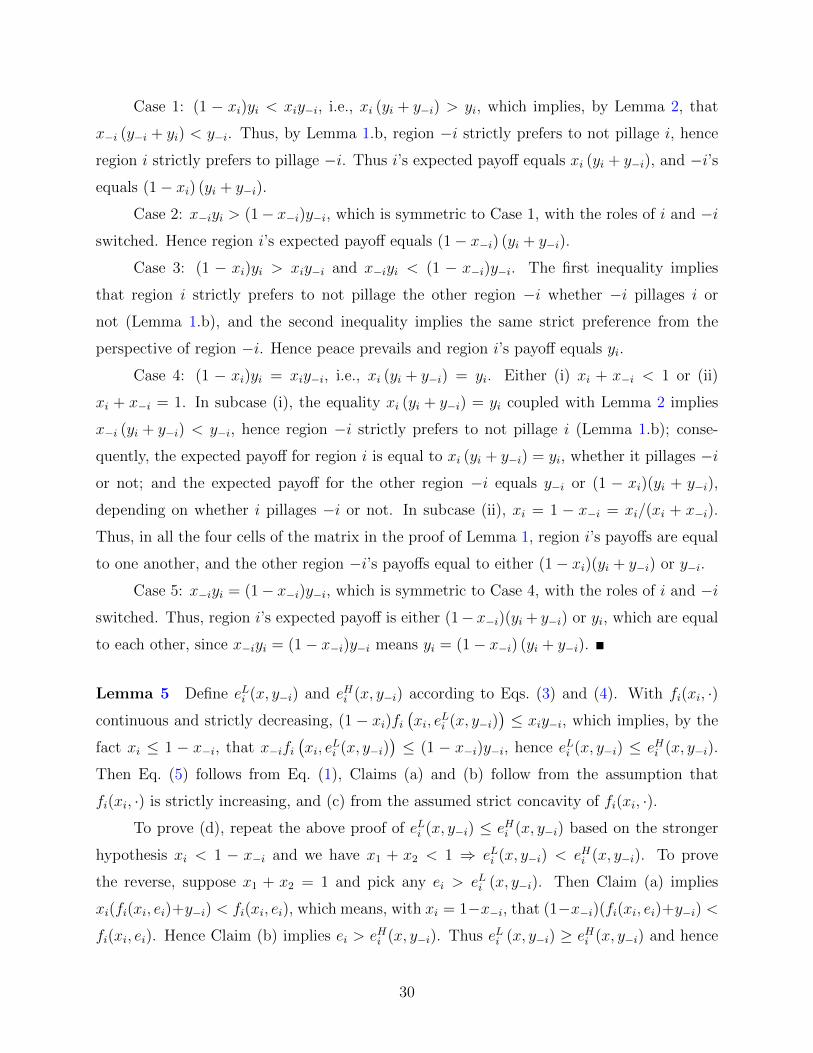
is depicted in Figure 1, where the cutoffs eLi and eHi are shorthands for

eLi (x, y−i) := inf {ei ∈ R+ : (1− xi)fi(xi, ei) ≥ xiy−i} , (3)

eHi (x, y−i) := sup {ei ∈ R+ : x−ifi(xi, ei) ≤ (1− x−i)y−i} . (4)

These cutoffs are determined by the anticipated output y−i of the other region. For region i,

exerting an effort less than eLi (x, y−i) means that it plans to pillage −i in the endgame,

exerting effort above eHi (x, y−i) means that i expects to be pillaged by −i, and any effort

between the two cutoffs means peace. Such observation is formalized by the next lemma.

effort

payoff peace

peace

agressor

victim

victim

eLi eHi

xiy−i

(1 − x−i)y−i

Figure 1: The gross expected payoff for region i

Lemma 5 For any region i, power allocation x := (x1, x2), ei ∈ R+ and y−i ∈ R++, there

exist thresholds eLi (x, y−i) and eHi (x, y−i), with eLi (x, y−i) ≤ eHi (x, y−i), such that

f ∗i (x, ei, y−i) =

xi (fi(xi, ei) + y−i) if ei ≤ eLi (x, y−i)

fi(xi, ei) if eLi (x, y−i) ≤ ei ≤ eHi (x, y−i)

(1− x−i) (fi(xi, ei) + y−i) if ei ≥ eHi (x, y−i)

(5)

and the following properties are true:

a. ei < (resp., ≤, >) eLi (x, y−i)⇐⇒ xi (fi(xi, ei) + y−i) > (resp., ≥, <) fi(xi, ei);

10

b. ei < (resp., ≤, >) eHi (x, y−i)⇐⇒ (1− x−i) (fi(xi, ei) + y−i) > (resp., ≥, <) fi(xi, ei);

c. f ∗i (x, ·, y−i) is strictly concave on[0, eLi (x, y−i)

], with a jump in its derivative at the

point eLi (x, y−i) if and only if eLi (x, y−i) < eHi (x, y−i), and is again strictly concave on[eLi (x, y−i),∞

);

d. x1 + x2 < 1⇐⇒ eLi (x, y−i) < eHi (x, y−i);

e. ei < (resp., ≤,=) eLi (x, y−i)⇐⇒ e−i > (resp., ≥,=) eH−i (x, yi).

Proof Appendix A.

3.3 Effort Levels That Are Possible Best Replies

A region has only two kinds of possible best responses, one being an optimal effort level

when it anticipates peace, and the other optimal when it anticipates war. Figure 2 depicts

one of such cases, where the supporting hyperplane at a peace-anticipating effort level ψi(xi)

happens to be higher than the one at a pillage-planning effort level ηi(xi), so the region’s best

response is ψi(xi). However, even a small change in the power allocation (x1, x2) or the other

region’s anticipated output y−i may alter the relative position between the two supporting

hyperplanes, switching the region’s best response discontinuously from a peace-anticipating

effort level to a war-anticipating one. Following are useful facts of the comparative statics

of both kinds of possible best responses, which we shall see are special cases of a function

γi : [0, 1]2 → R+ defined by, for any (xi, zi) ∈ [0, 1]2,

{γi(xi, zi)} := arg maxei∈R+

zifi(xi, ei)− ciei. (6)

Lemma 6 For each i ∈ {1, 2}:

a. for any (xi, zi) ∈ [0, 1]2, γi(xi, zi) defined by Eq. (6) exists and is unique;

b. for any xi ∈ [0, 1] there exists ζi(xi) ∈ [0, 1) such that if zi ≤ ζi(xi) then γi(xi, zi) = 0,

and if zi > ζi(xi) then γi(xi, zi) > 0 and ziD2fi (xi, γi(xi, zi)) = ci;

c. γi(xi, zi) is weakly increasing in (xi, zi), and strictly increasing in zi if zi > ζi(xi);

d. γi is continuous on [0, 1[2.

11

effort

payoff

eLi eHiηi(xi) ψi(xi)

slope = ci

Figure 2: ψi(xi) = γi(xi, 1); ηi(xi) = γi(xi, xi)

Proof Appendix A.

Lemma 6 applied to the cases z = 1 and z = xi gives Lemma 7, whose proof we omit.

Lemma 7 For each i ∈ {1, 2} and any xi ∈ [0, 1] there exist a unique ψi(xi) ∈ R++ and a

unique ηi(xi) ∈ R+ such that, for any y−i ∈ R+,

{ψi(xi)} = arg maxei∈R+

fi(xi, ei)− ciei, (7)

{ηi(xi)} = arg maxei∈R+

xi (fi(xi, ei) + y−i)− ciei, (8)

ci = D2fi(xi, ψi(xi)), (9)

and ψi and ηi are each continuous.

For each region i ∈ {1, 2}, the following inequalities are true for any xi ∈ [0, 1), and

the equalities true for any xi ∈ [0, 1] and any y−i ∈ R+. They are proved in Appendix A.

ψi(xi) > ηi(xi), (10)

fi (xi, ψi(xi))− ciψi(xi) > fi (xi, ηi(xi))− ciηi(xi), (11)

d

dxiψi(xi) = −D1D2fi(xi, ψi(xi))

D22fi(xi, ψi(xi))

, (12)

d

dxi(fi (xi, ψi(xi))− ciψi(xi)) = D1fi(xi, ψi(xi)) > 0. (13)

12

4 Decentralization

To characterize the social-surplus maximums among all possible power allocations, we dis-

sect the entire family of allocation-equilibrium pairs into two, one consisting of all warring

systems, and the other all peaceful systems. Our tractable characterization of the first set is

due to an observation that, as far as social surplus concerns, warring systems are equivalent

to fully decentralized ones.

4.1 Full Decentralization Means War

A consequence of full decentralization, giving all power to the regions, is internal warfare.

During the production phase, as formalized in the next lemma and proposition, any effort

level that a region chooses to exert will render the region either an aggressor or victim in

the endgame, except for the threshold effort level at which the region is indifferent between

war and peace. But the threshold effort level becomes a region’s best reply only when the

region’s decision is equivalent to the case as if it is expecting war.

Lemma 8 Given any fully decentralized power allocation x := (x1, x2) and any quantity

y−i ∈ R+ of output that region −i will produce, f ∗i (x, ·, y−i) = xi (fi(xi, ·) + y−i) on R+.

Proof Since x1 +x2 = 1 by definition of full decentralization, the top and bottom branches

of Eq. (1) coincide. To complete the proof, pick any ei for which the middle branch applies,

i.e., when (2) holds. With x1 + x2 = 1, (2) is reduced to (1− xi)fi(xi, ei) = xiy−i, i.e.,

fi(xi, ei) = xi(fi(xi, ei) + y−i) = (1− x−i)(fi(xi, ei) + y−i).

Hence at any such ei Eq. (1) implies that all of its three branches coincide.

The next proposition is attributed to Thomas Hobbes [21] for his bleak picture of the

state of nature, or full decentralization in our model.15

Proposition 1 (Hobbes) Any fully decentralized power allocation (x1, x2) admits a war-

ring equilibrium and admits no other equilibrium with a different outcome in effort or output.

15 “[D]uring the time men live without a common power to keep them all in awe, they are in that condition

which is called war, and such a war as is of every man against every man” (Hobbes [21, Chapter 13, p389]).

13

Proof Since (x1, x2) is fully decentralized, Lemma 8 implies that each region i’s effort

decision is the one in Eq. (8), which by Lemma 7 has a unique solution ηi(xi), which in turn

determines uniquely the output of region i. That proves the uniqueness claim. To prove

existence of a warring equilibrium, note from Lemma 5.d that eLi (x, y−i) = eHi (x, y−i) for

any y−i ∈ R+ and any i ∈ {1, 2}. Thus, for each i and any ei ∈ R+, either ei ≤ eLi (x, y−i) or

ei ≥ eHi (x, y−i). Therefore, by Lemma 2 and Eqs. (3)–(4), for any (e1, e2) ∈ R2+, with ensuing

outputs (y1, y2), there is an i ∈ {1, 2} for whom (1− xi)yi ≤ xiy−i and x−iyi ≥ (1− x−i)y−i.Hence it is an equilibrium in the endgame that region −i pillages region i, and i stays put

(the payoff matrix at Lemma 1).

4.2 War, at Best, Means Full Decentralization

Other than full decentralization, there is a myriad of systems, with various degrees of cen-

tralization, some resulting in peace, and others in war. The next proposition reduces the

complexity by asserting that among the alternatives of full decentralization we need only to

consider those that do not necessarily result in wars. Coupled with Lemma 3, this propo-

sition implies that in maximizing social surplus among warring systems we need only to

consider fully decentralized ones.

Proposition 2 For any allocation-equilibrium pair (x1, x2, e1, e2) such that x1 + x2 < 1 and

war occurs for sure, there exists another allocation-equilibrium pair (x′1, x′2, e′1, e′2) such that

x′1 + x′2 = 1 and it generates a larger social surplus.

Proof Let (x1, x2, e1, e2) be a warring system, with x1 + x2 < 1 and say region 1 pillaging

region 2 at equilibrium. Since x1 + x2 < 1, eLi (x, f−i(x−i, e−i)) < eHi (x, f−i(x−i, e−i)) for

each i ∈ {1, 2} (Lemma 5.d); as region 1 is the aggressor, e1 < eL1 (x, f2(x2, e2)), which by

Lemma 5.e implies e2 > eH2 (x, f1(x1, e1)). Thus, the effort e1 of the aggressor solves the

problem in Eq. (8) and so e1 = η1(x1) by Lemma 7; and the effort e2 of region 2 solves

maxe′′2∈R+

(1− x1) (f2(x2, e′′2) + y1)− c2e

′′2, (14)

which implies e2 = γ2(x2, 1− x1) by Eq. (6).

Consider a fully decentralized power allocation (x′1, x′2) such that x′1 := x1 and x′2 :=

1− x1 (hence > x2). With x′1 + x′2 = 1, Lemma 8 implies that the expected payoff function

14

for each region i ∈ {1, 2} becomes the differentiable and strictly concave function e′′i 7→x′i(fi(x

′i, e′′i ) + y′−i

)− cie′′i (given any y′−i). That means, for region 1, the objective function

becomes x′1 (fi(x′1, e′′1) + y′2)−c1e

′′1 = x1 (fi(x1, e

′′1) + y′2)−c1e

′′1 since x′1 = x1, hence its decision

problem is again equivalent to the one in Eq. (8), as in the previous power allocation (x1, x2).

Thus, e1 remains to be region 1’s best response under (x′1, x′2).

Now that region 1’s output remains unchanged as before, say denoted by y1, region 2’s

expected payoff from exerting effort e′′2 becomes

x′2(f2(x′2, e′′2) + y1)− c2e

′′2 = (1− x1)(f2(x′2, e

′′2) + y1)− c2e

′′2,

as x′2 = 1 − x1. Thus, given allocation (x′1, x′2) region 2’s best response e′2 = γ2(x′2, 1 − x1)

by Eq. (6). Since γ2(·, 1 − x1) is weakly increasing (Lemma 6.c), e′2 = γ2(x′2, 1 − x1) ≥γ2(x2, 1− x1) = e2. Thus, with x′2 > x2 and f2 assumed strictly increasing,

f2(x′2, e′2) > f2(x2, e2). (15)

With γ2(x′2, ·) weakly increasing (Lemma 6.c), e′2 = γ2(x′2, 1 − x1) ≤ γ2(x′2, 1). Hence

γ2(x′2, 1) ≥ e′2 ≥ e2. This, coupled with the fact that γ2(x′2, 1) is the unique maximum

(Lemma 6.a) of the strictly concave function e′′2 7→ f2(x′2, e′′2)− c2e

′′2, implies that

e′2 > e2 ⇒ f2(x′2, e′2)− c2e

′2 > f2(x′2, e2)− c2e2.

Consequently, since e′2 ≥ e2 and f2(·, e2) is strictly increasing,

e′2 6= e2 =⇒ f2(x′2, e′2)− c2e

′2 > f2(x2, e2)− c2e2. (16)

Eqs. (15) and (16), combined with the fact (x′1, e′1) = (x1, e1), imply the desired conclusion

f1(x′1, e′1)− c1e

′1 + f2(x′2, e

′2)− c2e

′2 > f1(x1, e1)− c1e1 + f2(x2, e2)− c2e2. �

4.3 Optimal Decentralization

By Propositions 1 and 2 and Lemma 3, maximizing social surplus among warring systems is

equivalent to maximizing social surplus among fully decentralized ones, which is a relatively

simple maximization problem with only a unidimensional choice variable.

15

Theorem 1 A system that maximizes the social surplus among warring allocation-equilibrium

pairs exists and is also the social surplus maximum among fully decentralized systems; it is

a power allocation (x∗1, 1− x∗1) such that x∗1 solves the problem

maxx1∈[0,1]

f1(x1, η1(x1))− c1η1(x1) + f2 (1− x1, η2(1− x1))− c2η2(1− x1). (17)

Proof By Propositions 1 and 2 and Lemma 3, any optimum among the warring allocation-

equilibrium pairs is the solution of

max(x1,x2;e1,e2)∈[0,1]2×R2

+

2∑i=1

(fi(xi, ei)− ciei)

subject to x1 + x2 = 1,

∀i ∈ {1, 2} : ei ∈ arg maxe′i∈R+

(xi (fi(xi, e′i) + f−i(x−i, e−i))− cie′i) ,

with the second constraint equivalent to the equilibrium condition because a region’s pay-

off function given a fully decentralized power allocation collapses to the one in the above

constraint due to Lemma 8. By Eq. (8), this constraint is the same as ei = ηi(xi) for each

i ∈ {1, 2}. Thus, the optimization problem is equivalent to (17). With fi continuous by

assumption and ηi continuous by Lemma 7, the solution for this problem exists.

5 Centralization

By Theorem 1, to seek better alternatives to warring systems, and better alternatives to full

decentralization, we need only to consider peaceful systems that are not fully decentralized.

5.1 Characterization of Peaceful Centralized Systems

For peace to prevail in the endgame, each region must, during the production phase, find

it a best response to exert an amount of effort such that the ensuing output preempts the

pillage incentive. Obviously such an effort level needs to maximize a region’s expected payoff

provided that peace will prevail, i.e., to solve the problem in (7). That however does not

suffice a best response for the region, because its expected payoff is not a concave function

of its effort (Lemma 5.c). The next proposition characterizes the condition for peace as

Ineq. (18), which is essentially a region’s incentive feasibility condition of not deviating to

another effort level with a plan to pillage the other region in the endgame.

16

Proposition 3 A power allocation (x1, x2) admits a peaceful equilibrium and is not fully

decentralized if and only if, for each i ∈ {1, 2},

fi (xi, ψi(xi))− ciψi(xi) ≥ xi (fi (xi, ηi(xi)) + f−i (x−i, ψ−i(x−i)))− ciηi(xi). (18)

Proof To prove the “only if” part, note that if (e1, e2) constitutes a peaceful equilibrium

given allocation (x1, x2) then each region i’s equilibrium effort ei belongs to the interval on

which i’s gross payoff function f ∗i (x1, x2, ·, f−i(x−i, e−i)) = fi(xi, ·). If, in addition, (x1, x2)

is not fully decentralized, i.e, x1 + x2 < 1, then this interval is nondegenerate (Lemma 5.d).

Then ei is a maximum of the function e′i 7→ fi(xi, e′i)− cie′i on a nondegenerate interval and

hence, with the function concave, on the entire R+. Thus ei = ψi(xi) by Eq. (7). Thus,

if (18) is not satisfied then region i would deviate to exert effort ηi(xi) and then pillage −i.To prove the “if” part, we first prove that (18) implies that (x1, x2) is not fully decen-

tralized. To prove that, recall from Eq. (8) the fact that ηi(xi) maximizes

xi (fi (xi, e′i) + f−i (x−i, ψ−i(x−i)))− cie′i

among all e′i ∈ R+. Hence (18) implies

fi (xi, ψi(xi))− ciψi(xi) ≥ xi (fi (xi, ηi(xi)) + f−i (x−i, ψ−i(x−i)))− ciηi(xi)

≥ xi (fi (xi, ψi(xi)) + f−i (x−i, ψ−i(x−i)))− ciψi(xi). (19)

Analogously we obtain an inequality for −i. Summing these two inequalities we have

f1 (x1, ψ1(x1))− c1ψ1(x1) + f2 (x2, ψ2(x2))− c2ψ2(x2)

≥ x1 (f1 (x1, η1(x1)) + f2 (x2, ψ2(x2)))− c1η1(x1) + x2 (f2 (xi, η2(x2)) + f1 (x1, ψ1(x1)))− c2η2(x2)

≥ x1 (f1 (x1, ψ1(x1)) + f2 (x2, ψ2(x2)))− c1ψ1(x1) + x2 (f2 (x2, ψ2(x2)) + f1 (x1, ψ1(x1)))− c2ψ2(x2).

If the allocation (x1, x2) is fully decentralized, i.e., x1 +x2 = 1, then the last line of the above

formula is equal to the first line. Consequently, for each i ∈ {1, 2},

xi (fi (xi, ηi(xi)) + f−i (x−i, ψ−i(x−i)))− ciηi(xi) = xi (fi (xi, ψi(xi)) + f−i (x−i, ψ−i(x−i)))− ciψi(xi),

which implies, with Ineq. (10) true for all xi ∈ [0, 1), that xi = 1. But that cannot be a

feasible power allocation for both regions i, a contradiction.

To complete the proof for the “if” part, let ei := ψi(xi) for each i and we claim that

(e1, e2) constitutes a peaceful equilibrium given (x1, x2). We first note that, given the outputs

17

produced by such effort levels, with yj := fj(xj, ej) for each j ∈ {1, 2}, each region finds it a

best response to not pillage the other. That is because, for each i ∈ {1, 2}, Ineq. (19) implies

yi − xi(yi + y−i) ≥ ci (ψi(xi)− ψi(xi)) = 0,

which in turn implies, by Lemma 1.b, that i weakly prefers to not pillage−i. Next we show for

each i that ei maximizes region i’s expected payoff f ∗i (x1, x2, e′′i , y−i)−cie′′i among all e′′i ∈ R+.

First, since it is a best response for each region to not pillage the other given (x1, x2, e1, e2),

Lemma 4 implies for each i that ei belongs to the domain on which f ∗i (x, ·, y−i) = fi(xi, ·);this domain, by Eq. (5), is the interval

[eLi (x1, x2, y−i) , e

Hi (x1, x2, y−i)

]. Consequently, ei,

by its definition ei := ψi(xi) and Eq. (7), is a maximum of f ∗i (x, e′′i , y−i)− cie′′i among all e′′i

in this interval. The optimality of ei is then extended to the interval[eHi (x1, x2, y−i) ,∞

),

because the derivative of f ∗i (x, ·, y−i) drops at eHi (x1, x2, y−i) and then keeps decreasing on

this interval (Lemma 5.c). Thus, the optimality of ei is further extended to the entire R+

due to Ineq. (18) and the definition of ηi(xi). Hence ei best replies e−i, as claimed.

Lemma 9 For any i ∈ {1, 2}, if xi = 0 then Ineq. (18) holds strictly.

Proof With xi = 0, the right-hand side of (18) is always nonpositive. The left-hand side,

by contrast, is always strictly positive: Instead of exerting effort ψi(xi), region i could have

chosen zero effort thereby ensuring a net payoff fi(xi, 0)−ci·0 ≥ 0; but the fact that ψi(xi) > 0

(Lemma 7) and that it is the unique solution for (7) implies fi(xi, ψi(xi)) − ciψi(xi) >

fi(xi, 0) ≥ 0. Thus, Ineq. (18) holds strictly, as claimed.

Corollary 1 (possibility of peace) There exists a power allocation, not fully decentral-

ized, that admits a peaceful equilibrium.

Proof By Lemma 9 and Proposition 3, (0, 0) is such a power allocation.

5.2 Optimal Centralization

While peaceful equilibrium is achievable through some centralized allocation (Corollary 1),

centralization would not do much good if the best it could offer is the totally centralized

allocation (0, 0) in the proof of Corollary 1, which, like Hobbes’s [21] Leviathan, maintains

internal peace through depriving the regions of any power that could have helped the pro-

duction. This subsection is hence devoted to characterization of the social-surplus optimum

18

among peaceful systems that are not fully decentralized. As a corollary of the characteriza-

tion, not only can other centralized systems do better than the Leviathan, total centraliza-

tion, such Leviathan is also the worst among all peaceful, centralized systems. Furthermore,

optimal centralization systems can be bounded away from total centralization even when

power allocated to the regions is arbitrarily insignificant to production.

Lemma 10 A system that maximizes the social surplus among peaceful allocation-equilibrium

pairs that are not fully decentralized corresponds to a power allocation (x∗1, x∗2) that solves

max(x1,x2)∈[0,1]2

2∑i=1

(fi(xi, ψi(xi)− ciψi(xi)) (20)

subject to x1 + x2 ≤ 1

(18) holds ∀i ∈ {1, 2}.

Proof The constraint x1+x2 ≤ 1 is merely the feasibility condition for (x1, x2) to be a power

allocation. By Proposition 3, the constraint that (18) holds for each region i is the sufficient

and necessary condition for a (feasible) power allocation to constitute a peaceful system that

is not fully decentralized. Given that the allocation (x1, x2) is not fully decentralized, there

is a nondegenerate interval on which a region’s payoff function f ∗i (x, ·, y−i) is equal to fi(xi, ·)(Lemma 5.d). Thus, by Eq. (7), ψi(xi) is equal to region i’s equilibrium effort level, and

hence the effort level in the objective function.

The next theorem asserts existence of a social-surplus maximum among peaceful sys-

tems that are not fully decentralized. That might sound surprising, as the qualification

“not fully decentralized,” x1 + x2 < 1, sounds as if the feasibility set for the maximization

problem (20) were an open set. Actually it is a closed set because, by Proposition 3, any

(x1, x2) ∈ [0, 1]2 that satisfies (18) for each i also satisfies the strict inequality x1 + x2 < 1.

Theorem 2 There exists a social-surplus maximum (xi, ψi(xi))2i=1 among all peaceful allocation-

equilibrium pairs that are not fully decentralized, and (xi)2i=1 can only be:

i. a solution of the following equation for each i ∈ {1, 2},

fi(xi, ψi(xi))− ciψi(xi) = xi (fi(xi, ηi(xi)) + f−i(x−i, ψ−i(x−i)))− ciηi(xi), (21)

ii. or a solution of Eq. (21) for some i ∈ {1, 2} and (xi, x−i) is a tangent point between the

graph generated by Eq. (21) and an indifference curve of the objective function (20),

19

iii. or x−i = 0 for some i ∈ {1, 2} and (xi, 0) is a solution of Eq. (21).

Proof Appendix B.

The Hobbesian Leviathan is the worst centralized system:

Corollary 2 Total centralization, (0, 0), is not an optimum among peaceful systems that are

not fully decentralized. Furthermore, any other peaceful systems that is not fully decentralized

generates a larger social surplus than total centralization.

Proof By Theorem 2, at any optimal centralized system Eq. (21) for some i ∈ {1, 2} holds,

whereas by Lemma 9 neither holds at (0, 0). Hence (0, 0) is suboptimal. For the second half

of the corollary, pick any other peaceful systems (xi, ψi(xi))2i=1 that is not fully decentralized.

Then xi ≥ 0 for both i and xi > 0 for at least one i. By the inequality in (13), the social

surplus generated by (xi, ψi(xi))2i=1 is larger than that generated by (0, 0, ψ1(0), ψ2(0)).

While total centralization is suboptimal, can it be nearly optimal under some parameter

values? Casting a doubt on such possibility is the next corollary of Theorem 2, giving a lower

bound of the total regional power at an optimum.

Corollary 3 For each i ∈ {1, 2} there exists a strictly positive constant

ρi :=fi(0, ψi(0))− ciψi(0)

fi(1, ψi(1) + f−i(1, ψ−i(1))(22)

such that, for any optimal centralized allocation (x1, x2), xi > ρi for at least one i ∈ {1, 2},and the inequality holds for both i if (x1, x2) belongs to Case (i) in Theorem 2.

Proof Appendix B.

The lower bound of regional power given in Corollary 3 can be bounded away from

zero even when regional power becomes arbitrarily less significant than efforts to the region’s

production, in terms of the technical rate of substitution between power and efforts:

Remark 1 There exists a sequence (fn1 , fn2 )∞i=1 of environments such that the lower bound

in Corollary 3 is bounded away from zero while the technical rate of substitution

limn→∞

D1fni (xi, ei)

−D2fni (xi, ei)= 0.

for each i ∈ {1, 2} and for any (xi, ei) ∈ [0, 1]× R+.

Proof Appendix B.

20

5.3 Productivity and Decentralization

Within this subsection, let us specialize to a symmetric environment such that

f1 = f2 = f and c1 = c2 = c (23)

for some function f and effort cost c satisfying the assumptions in Section 2. To see how

the optimal degree of centralization may vary with the productive capability of a society, let

us parameterize the latter by an index t ∈ T , for some compact interval T , such that the

output produced by a region i, with power xi and effort ei, is equal to f(xi, ei; t) with

D3f > 0, D3D1f ≥ 0 and D3D2f ≥ 0. (24)

Within this subsection we consider only symmetric allocations, where the two regions,

identical in their primitives, are allocated an identical amount of power. Both regions given

the production function f(·, ·; t), let x(t) denote any social-surplus maximizer among all

symmetric allocations that are peaceful and not fully decentralized. For any x ∈ [0, 1/2], let

ψ(x, t) and η(x, t) denote, respectively, the ψi(xi) and ηi(xi) defined in Eqs. (7)–(8), with

the production function fi there being f(·, ·; t), and xi being x. For any continuous function

g : [0, 1/2]× R+ × T → R, denote

‖g‖sup := sup(x,e,t)∈[0,1/2]×[η(x,t),ψ(x,t)]×T

g (x, e, t)

and likewise for ‖g‖inf .

Theorem 3 If both (23) and (24) are satisfied and if

c

‖ −D22f‖inf

‖D3D2f‖sup ≤ ‖ψ − η‖inf‖D3D2f‖inf , (25)

then t′′ > t′ implies x(t′′) > x(t′).

Proof Appendix C

The intuition for the theorem is that the additional output of a region due to productiv-

ity improvements is fully owned by the region itself only if there is no internal warfare. Thus,

expansions in productive capabilities may strengthen a region’s preference of peace over war,

thereby relaxing its incentive constraint and hence allowing more power to be delegated to

the region without upsetting peace. The only countervailing effect is that the productivity

21

improvement may enlarge the other region’s output by so much that this region would rather

shirk in its production and then pillage the enriched neighbor. Ineq. (25) assumed in the

theorem is to ensure that such countervailing effect is dominated. The inequality requires

that D3D2f , the complementarity between efforts and the productivity shock, vary suffi-

ciently little and the marginal product of effort, D2f , diminish sufficiently quickly as effort

increases. For example, consider a case where (x, e) is additively separable from the produc-

tivity shock t, with t interpreted as an increase in natural endowments for the society such

as a newfound colony. It is perhaps no accident that the “discovery” of America occurred

merely decades before the Reformation, dissecting the Christendom in Western Europe.

6 The Optimality of Centralization

Since our model is even-handed on the pros and cons of centralization versus decentralization,

it is natural that, when we compare the optimum among centralized systems with that among

decentralized ones, the outcome depends on the values of the parameters.

Remark 2 Suppose the two regions have an identical effort cost c > 0 and f1 = f2 = f for

some common production function f parameterized by α ≥ 0, β ≥ 0, θ > 0 and τ ∈ (0, 1).16

a. If f is defined by, for any xi ∈ [0, 1] and any ei ∈ R+,

f(xi, ei) :=√

(xi + α)ei, (26)

the optimal decentralized system generates larger social surplus than the optimal cen-

tralized system when α = 0, and the opposite is true when α > 3− 2√

2.

b. If f is defined by, for any xi ∈ [0, 1] and any ei ∈ R+,

f(xi, ei) := (θxi)β eτi , (27)

the optimal decentralized system yields larger social surplus than the optimal centralized

system when β + τ ≥ 1, and the opposite is true when β/(1− τ) is sufficiently small.

16 Like Cobb-Douglas functions, the production functions in this remark satisfy all assumptions stated in

Section 2 except the Inada condition limei↓0D2f(0, ei) > c at xi = 0.

22

Proof Appendix D.

To provide a normative foundation of centralization, the next Theorem 4 implies that,

when the marginal product of power and the complementarity between power and efforts

become sufficiently small, some degree of centralization generates larger social surplus than

any fully decentralized system.

To illustrate the intuition, suppose that a fully decentralized power allocation (x∗1, x∗2)

is replaced by an allocation (x1, x2) that sustains peace and is not fully decentralized. The

net gain thereof in the social surplus generated from region i ∈ {1, 2} is equal to

∆i(xi, x∗i ) := fi (xi, ψi(xi))− ciψi(xi)− fi (x∗i , ηi(x∗i )) + ciηi(x

∗i ). (28)

To analyze this difference, recall the function γi(xi, zi) defined in Eq. (6) and the fact that

ψi(xi) = γi(xi, 1) and ηi(xi) = γi(xi, xi). Thus,

∆i(xi, x∗i ) = ∆s

i (xi, x∗i ) + ∆p

i (xi, x∗i ), (29)

where

∆si (xi, x

∗i ) := fi (xi, γi(xi, 1))− ciγi(xi, 1)− fi (xi, γi(xi, x∗i )) + ciγi(xi, x

∗i ),

∆pi (xi, x

∗i ) := fi (xi, γi(xi, x

∗i ))− ciγi(xi, x∗i )− fi (x∗i , γi(x∗i , x∗i )) + ciγi(x

∗i , x∗i ),

with ∆si (xi, x

∗i ) measuring the security effect of increasing the probability, with which region i

keeps its own output, from x∗i to one, and ∆pi (xi, x

∗i ) the disempowerment effect of changing

the power allocated to region i from x∗i to xi. Unless x∗i ≤ xi, the two effects are opposite

to each other, and the centralized system (x1, x2) outperforms the decentralized (x∗1, x∗2) if

the security effect outweighs the disempowerment effect. One readily sees that the former

effect is large when the marginal product of efforts is large with the effort level ranging from

γi(xi, x∗i ) to γi(xi, 1), while the latter effect is large in absolute value when the marginal

product of power, due to the direct effect D1fi of power and its indirect effect D1D2fi on

the marginal product of efforts, is large with the amount of power ranging from x∗i to xi.

Thus, when D1fi and D1D2fi are uniformly small enough, the disempowerment effect is

outweighed by the security effect, and decentralization outperformed by centralization.

Theorem 4 For any sequence (fn1 , fn2 )∞n=1 of environments such that, for each n and each i,

limei↓0D2fni (xi, ei) = ∞ for any xi ∈ (0, 1], if for each i ∈ {1, 2} there exist ri > 0 and

23

bi > 0 such that, with ρni defined by (22) and γni defined by (6),

lim infn→∞

ρni > ri, (30)

limn→∞

max(xi,zi)∈[min{ri,1/2},1]2

D1D2fni (xi, γ

ni (xi, zi)) = 0, (31)

limn→∞

max(xi,zi)∈[min{ri,1/2},1]2

D1fni (xi, γ

ni (xi, zi))

∣∣D22f

ni (xi, γ

ni (xi, zi))

∣∣ = 0, (32)

limn→∞

max(xi,zi)∈[min{ri,1/2},1]2 |D22f

ni (xi, γ

ni (xi, zi))|

min(xi,zi)∈[min{ri,1/2},1]2 |D22f

ni (xi, γni (xi, zi))|

< bi, (33)

then, for all sufficiently large n, the maximum social surplus among peaceful centralized

systems given (fn1 , fn2 ) is strictly larger than the maximum social surplus among fully decen-

tralized ones given (fn1 , fn2 ).

Proof Appendix E.

In Theorem 4, the Inada condition of fi(xi, ·) for all xi > 0 ensures that a region’s

optimal efforts such as ηi(xi) and γi(xi, zi) be interior solutions and hence differentiable for

all xi > 0. The hypothesis (30), coupled with Corollary 3, guarantees that at the optimal

centralized system the power in at least one region is bounded away from zero, the possible

singularity point for a region’s optimal effort. The other hypotheses concern the marginal

effect of power versus efforts, with the effort level ranging along the path γni determined by

the primitives. Eq. (31) requires that the complementarity between power and efforts be

sufficiently small. Eq. (32) requires that the marginal product of power and the decay rate

of the marginal product of efforts be sufficiently orthogonal to each other; in particular, the

equation is satisfied if the marginal product of power is sufficiently small. Ineq. (33) imposes

an upper bound on the variation of the decay rate of the marginal product of efforts.

All hypotheses of the theorem are satisfied by the example defined by Eq. (26) in

Remark 2 when α > 0, with n being the α there. For the example defined by Eq. (27) to

satisfy all the hypotheses, we need only to amend its definition by translating the production

function by a positive constant so that f(0, ψ(0)) > 0. One can then verify all the hypotheses,

with 1/(1− τ) and (1− τ)/β going to infinity when n→∞.17

17 Let us illustrate with the function fi defined by Eq. (26) for any α > 0. It satisfies the Inada

condition because D2fi(xi, ei) = (1/2)√

(xi + α)/ei and α > 0. The proof of Remark 1 has verified

Ineq. (30), with ri ∈ (0, c−i/(2(c1 + c2))). To verify (31)–(33), note that γi(xi, zi) = (xi + α)z2i /(4c2i ).

Hence D1fi(xi, γi(xi, zi)) = zi/(4ci), D1D2fi(xi, γi(xi, zi)) = ci/ (2zi(xi + α)), D22fi (xi, γi(xi, zi)) =

24

7 Greedy Center

While Theorem 4 has demonstrated a normative justfication to keep some power away from

the productive regions thereby maintaining internal peace, the center with such power might

exploit its advantage to extort outputs from the regions. We shall modify the model to

contrast a case where the center has no commitment power to another case where it has.

Whereas the relative merit of centralization is gone in the former, not all is lost in the latter.

7.1 A Case of an Extortive Center

Let us modify the model so that, when internal warfare does not occur, with power allocation

(x1, x2) and realized outputs (y1, y2), the center chooses an s ∈ [0, 1] and demands each region

to transfers a share s of its output to the center. If both regions disobey the order, a war

breaks out between their joint force and the center, and the center wins with probability

1− x1 − x2; if the center wins then the center gets all the outputs, y1 + y2, else each region

retains its own output. If only region i disobeys the order then the war breaks out between i

and the center, and the center wins with probability (1− x1− x2)/(1− x−i), and the winner

gets the entire output yi of region i, leaving zero to the loser. In the event of internal warfare

between the two regions, no transfer is made from any region to the center.

Proposition 4 In this model, given any power allocation that is not fully decentralized,

internal warfare occurs at equilibrium and the center receives zero revenue from the regions.

Proof With the power allocation not fully decentralized, 1 > x1+x2, a region i’s probability

of defeating the center if it revolts by itself, xi/(1−x−i), is less than its probability of defeating

the center if it revolts together with the other region, x1 + x2. Thus, each region prefers to

be united in revolting against the center. Furthermore, in the event of a united revolt, each

region i’s payoff calculation is the same: it wins with probability x1 + x2, and if it wins it

gets yi; whereas if it does not revolt then it gets yi(1− s). Thus, the center expects no revolt

from the regions if and only if 1− s ≥ x1 + x2. It follows that the share s of the output that

−2c3i /(z3i (xi + α)

), and D1fi(xi, γi(xi, zi))D

22fi(xi, γi(xi, zi)) = −c2i /

(2z2i (xi + α)

). Thus (31) and (32)

follow, with α playing the role of n. To verify (33), note that, for any r ∈ (0, 1), the maximum of∣∣D22fi(xi, γi(xi, zi))

∣∣, among all (xi, zi) ∈ [r, 1]2, is equal to 2c3i /(r3α), and the minimum equal to 2c3i /(1+α);

hence the ratio between the two is (1 + α)/(r3α), which converges to a finite number 1/r3 when α→∞.

25

the center would optimally choose to demand is equal to

s = 1− x1 − x2.

Consequently, a region i’s gross expected payoff is equal to xi (fi(xi, ei) + y−i) if it

plans to pillage the other region −i, equal to (x1 + x2)fi(xi, ei) if it expects peace, and

(1− x−i) (fi(xi, ei) + y−i) if it expects to be pillaged by −i. In particular, the gross payoff is

equal to the middle branch (x1 +x2)fi(xi, ei) only if not pillaging the other region constitutes

an equilibrium in the subgame given realized output pair (y1, y2):

x1 (y1 + y2) ≤ (x1 + x2)y1 and x2 (y1 + y2) ≤ (x1 + x2)y2.

Sum the two weak inequalities to obtain (x1 + x2)(y1 + y2) ≤ (x1 + x2)(y1 + y2), which

forces both weak inequalities into equalities, i.e., xi(yi + y−i) = (x1 + x2)yi, or equivalently

xi (fi(xi, ei) + y−i) = (x1 + x2)fi(xi, ei), for each i ∈ {1, 2}. Given any y−i, this condition

holds for only one value of ei, denoted ePi (x, y−i), at which the graphs of the functions

(xi +x−i)fi(xi, ·) and xi (fi(xi, ·) + y−i) intersect. Thus, the interval of effort levels on which

peace prevails collapses into the point ePi (x, y−i), and region i’s gross expected payoff equals

f ∗i (x, ei, y−i) =

xi (fi(xi, ei) + y−i) if ei ≤ ePi (x, y−i)

(1− x−i) (fi(xi, ei) + y−i) if ei ≥ ePi (x, y−i).

Since xi < 1 − x−i, the function f ∗i (x, ·, y−i) is strictly concave on [0, ePi (x, y−i)] and on

[ePi (x, y−i),∞), with a jump of its derivative at the boundary ePi (x, y−i). Thus, region i’s

optimal effort is away from the point ePi (x, y−i), so the region will either pillage others or be

pillaged. With internal warfare occurring for sure, the center gets zero revenue.

Hence centralization with such an extortive center ends with a warring equilibrium,

which is wasteful by Proposition 2. The implication is that in order for centralization to

achieve what it is supposed to achieve, it is necessary to curb the arbitrariness of the center.

7.2 When the Selfish Center Can Commit

The negative observation in the previous subsection is partially due to the assumption that

the center does not commit to a tax rate at the outset. With the share of outputs demanded

after they are realized, the center would push its share to the limit as far as the centralized

26

power allows. If the center can commit, however, it may want to commit to a less draconian

tax rate thereby stimulating some efforts from the regions and reaping greater tax revenues.

Thus consider the following variant of the model: Once the power allocation (x1, x2) has

been determined, the center chooses a tax rate s ∈ [0, 1] to commit to, with s ≤ 1− x1− x2,

such that in the event of peace each region transfers a fraction s of its output to the center,

whereas in the event of internal warfare the center receives no transfer.

Consequently, a region i’s gross expected payoff, from exerting effort ei and expecting

the other region’s output y−i, is equal to xi (fi(xi, ei) + y−i) if it plans to pillage −i, or

(1− s)fi(xi, ei) if it expects peace, or (1− x−i) (fi(xi, ei) + y−i) if it expects to be pillaged.

Lemma 11 For any s ∈ [0, 1−x1−x2], if x−i > 0⇒ si < x−i for each −i, then a region i’s

gross expected payoff is

f ∗i (x, ei, y−i) =

xi (fi(xi, ei) + y−i) if ei ≤ eLi (x, y−i, s)

(1− s)fi(xi, ei) if eLi (x, y−i, s) ≤ ei ≤ eHi (x, y−i, s)

(1− x−i) (fi(xi, ei) + y−i) if ei ≥ eHi (x, y−i, s),

(34)

with the thresholds eLi (x, y−i, s) and eHi (x, y−i, s) defined analogously to eLi (x, y−i) and eHi (x, y−i)

in Eqs. (3) and (4) so that eHi (x, y−i, s) =∞ if x−i = 0.

Proof Appendix F.

Receiving zero tax revenue in the event of internal warfare, the center weakly prefers

a peaceful equilibrium to any warring one. At any peaceful equilibrium, each region i solves

maxe′i∈R+

(1− s)fi(xi, e′i)− cie′i, (35)

which, by Lemma 6, admits a unique solution, denoted by φi(xi, s), continuous in (xi, s), as

φi(xi, s) = γi(xi, 1− s). (36)

Based on analyses of φi, the next proposition says that, as long as the power allocation

admits a peaceful equilibrium without binding the incentive constraint in the original model,

peace is attainable in the current model despite a selfish center. Furthermore, the center’s

preference of peace over war is strict, and so is its preference of making a commitment.

Proposition 5 Given any power allocation (x1, x2) such that Ineq. (18) holds strictly for

each i ∈ {1, 2}, there exists s ∈ (0, 1 − x1 − x2] that admits a peaceful equilibrium in the

27

current model, and the center strictly prefers committing to such an s to no commitment or

any warring equilibrium.

Proof Appendix F.

To reap more tax revenues, the selfish center would commit to a tax rate less draconian

than in the previous subsection, thereby encouraging productive efforts from the regions.

Proposition 6 Given any power allocation (x1, x2) such that Ineq. (18) holds strictly for

each i ∈ {1, 2}, the center’s revenue-maximizing tax rate exists and belongs to (0, 1−x1−x2).

Proof Appendix F.

This modified model for simplicity gives all bargaining power to the selfish center.

Thus one would expect that in general the normative foundation of centralization is ruined

by such a greedy, powerful center. Yet the next remark says that there are cases where even

the best among decentralized systems is outperformed by even the worst centralized system,

the total centralization, where power is entirely taken from the regions by a selfish center,

who commits to a tax rate to maximize its own revenues.

Remark 3 Suppose, for each i ∈ {1, 2} and any (xi, ei) ∈ [0, 1]× R+,

fi(xi, ei) = ln(xi + 1) + 4 ln(ei + 1), (37)

with an effort cost c ∈ (0, 4) identical to both regions i. Then:

a. if c ∈ (0.36, 3.64) then, at the social-surplus maximum among fully decentralized sys-

tems, the power allocation either gives approximately 0.09 of the power to one region

and the rest to the other region, or gives each region 1/2 of the total power;

b. given the total centralization allocation, (0, 0), the center strictly prefers to commit to

a tax rate rather than choose it after the outputs have been produced;

c. there exists a nonempty nondegenerate set of values of c such that the optimal decen-

tralized system in (a) produces less social surplus than the total centralization, with the

center committing to a tax rate that maximizes the revenue extracted from the regions.

Proof Appendix G.

28

Centralization is costly, meant to maintain internal peace at the expense of individual

productivity. Total centralization, or the Hobbesian Leviathan, goes to the extreme of strip-

ping all power from social members. Such a tremendous cost is compounded by the avarice

of the center enjoying absolute power. Yet even such an extreme form of centralization can

sometimes outperform even the best among decentralized systems, says the above remark.

There, the center prefers to commit than not commit to a tax rate, because without com-

mitment the powerless regions would anticipate that all their outputs will be extorted by

the center and hence would exert no effort at all, rendering zero tax revenue for the center.

By a similar token, the center would rather commit to a tax rate that leaves the regions

an ample fraction of their outputs for them to exert efforts. When the marginal product of

efforts is sufficiently larger than that of power in this example, the social loss from depriving

the regions of their power is more than covered by the social gain from the efforts that the

regions exert in anticipation of internal peace.

Naturally one would ask whether a center’s commitment is credible and how it can be

made credible. As in Myerson [40], where the prince is assumed to be able to commit to

mechanisms that randomize the penalty on the governor, one could interpret the importance

of the commitment assumption as an implication that the theory points to the necessity

of institutionalized monitoring of the prince there, and the center here.18 Our model may

allow for extensions that incorporate such institutional structures of the center, thereby to

produce deeper assessments on the normative foundation of centralization.

A Proofs of Lemmas 4–6 and Formulas (10)–(13)

Lemma 4 In exerting effort ei region i incurs the sunk cost ciei and produces output

yi := fi(xi, ei). In the endgame given its output yi and the other’s y−i, region i’s (gross)

expected payoff is calculated below for each case listed on the right-hand side of Eq. (1).

18 Acemoglu and Robinson [4] regard the ruling elites’ lack of commitment ability to transfer their power

to the mass as a fundamental problem in undemocratic societies. In our setting, however, the commitment

is not about transferring power, but rather committing to a tax rate. There are anecdotes in history where

powerful rulers committed to their own policies. Examples include Shang Yang’s reform of the Qin Kingdom

in China around 350 BCE, where he implemented a strict penal code by applying it first to the nobles,

and Augustus’s implementation of his marriage laws, which he himself observed through adopting enough

children to meet the requirement of the laws and later exiling his own daughter for violation of the laws.

29

Case 1: (1 − xi)yi < xiy−i, i.e., xi (yi + y−i) > yi, which implies, by Lemma 2, that

x−i (y−i + yi) < y−i. Thus, by Lemma 1.b, region −i strictly prefers to not pillage i, hence

region i strictly prefers to pillage −i. Thus i’s expected payoff equals xi (yi + y−i), and −i’sequals (1− xi) (yi + y−i).

Case 2: x−iyi > (1− x−i)y−i, which is symmetric to Case 1, with the roles of i and −iswitched. Hence region i’s expected payoff equals (1− x−i) (yi + y−i).

Case 3: (1 − xi)yi > xiy−i and x−iyi < (1 − x−i)y−i. The first inequality implies

that region i strictly prefers to not pillage the other region −i whether −i pillages i or

not (Lemma 1.b), and the second inequality implies the same strict preference from the

perspective of region −i. Hence peace prevails and region i’s payoff equals yi.

Case 4: (1 − xi)yi = xiy−i, i.e., xi (yi + y−i) = yi. Either (i) xi + x−i < 1 or (ii)

xi + x−i = 1. In subcase (i), the equality xi (yi + y−i) = yi coupled with Lemma 2 implies

x−i (yi + y−i) < y−i, hence region −i strictly prefers to not pillage i (Lemma 1.b); conse-

quently, the expected payoff for region i is equal to xi (yi + y−i) = yi, whether it pillages −ior not; and the expected payoff for the other region −i equals y−i or (1 − xi)(yi + y−i),

depending on whether i pillages −i or not. In subcase (ii), xi = 1 − x−i = xi/(xi + x−i).

Thus, in all the four cells of the matrix in the proof of Lemma 1, region i’s payoffs are equal

to one another, and the other region −i’s payoffs equal to either (1− xi)(yi + y−i) or y−i.

Case 5: x−iyi = (1− x−i)y−i, which is symmetric to Case 4, with the roles of i and −iswitched. Thus, region i’s expected payoff is either (1− x−i)(yi + y−i) or yi, which are equal

to each other, since x−iyi = (1− x−i)y−i means yi = (1− x−i) (yi + y−i). �

Lemma 5 Define eLi (x, y−i) and eHi (x, y−i) according to Eqs. (3) and (4). With fi(xi, ·)continuous and strictly decreasing, (1 − xi)fi

(xi, e

Li (x, y−i)

)≤ xiy−i, which implies, by the

fact xi ≤ 1 − x−i, that x−ifi(xi, e

Li (x, y−i)

)≤ (1 − x−i)y−i, hence eLi (x, y−i) ≤ eHi (x, y−i).

Then Eq. (5) follows from Eq. (1), Claims (a) and (b) follow from the assumption that

fi(xi, ·) is strictly increasing, and (c) from the assumed strict concavity of fi(xi, ·).To prove (d), repeat the above proof of eLi (x, y−i) ≤ eHi (x, y−i) based on the stronger

hypothesis xi < 1 − x−i and we have x1 + x2 < 1 ⇒ eLi (x, y−i) < eHi (x, y−i). To prove

the reverse, suppose x1 + x2 = 1 and pick any ei > eLi (x, y−i). Then Claim (a) implies

xi(fi(xi, ei)+y−i) < fi(xi, ei), which means, with xi = 1−x−i, that (1−x−i)(fi(xi, ei)+y−i) <

fi(xi, ei). Hence Claim (b) implies ei > eHi (x, y−i). Thus eLi (x, y−i) ≥ eHi (x, y−i) and hence

30

eLi (x, y−i) = eHi (x, y−i). Thus x1 + x2 = 1⇒ eLi (x, y−i) = eHi (x, y−i), hence (d) follows.

To prove (e), note, by Claim (a), that ei < eLi (x, y−i) is equivalent to xi(yi + y−i) > yi,

i.e., (1 − xi)(yi + y−i) < y−i; that is equivalent to the condition that e−i (which pro-

duces y−i) belongs to the interval over which the function f−i(x−i, ·) is above the function

(1 − xi) (f−i(x−i, ·) + yi), which by Claim (b), with the roles of i and −i switched, is the

same as e−i > eH−i(x, yi). The proof of ei ≤ eLi (x, y−i)⇔ e−i ≥ eH−i (x, yi) is likewise, and so

is ei = eLi (x, y−i)⇔ e−i = eH−i (x, yi). �

Lemma 6 For Claim (a), uniqueness of the solution follows directly from the assumed strict

concavity of fi(xi, ·), and existence follows from the assumption that fi(xi, ·) is continuously

differentiable and limei→∞D2fi(xi, ei) < ci. To prove Claim (b), let

ζi(xi) := inf

{zi ∈ [0, 1] : lim

ei↓0ziD2fi(xi, ei) > ci

}.

Note ζi(xi) < 1 by the assumption limei↓0D2fi(xi, ei) > ci. Since D2fi(xi, ·) is assumed

strictly decreasing, if zi ≤ ζi(xi) then γi(xi, zi) = 0, and if zi > ζi(xi) then γi(xi, zi) > 0 and

the first-order condition ziD2fi (xi, γi(xi, zi)) = ci is satisfied. Hence Claim (b) is proved.

Next we claim that γi(xi, zi) is weakly increasing in (xi, zi). The reason is that the objective

function of the maximization problem in Eq. (6) exhibits increasing difference in (ei, xi),

because D1D2fi ≥ 0 by assumption, and increasing difference in (ei, zi), because D2fi > 0

by assumption. Thus, to prove Claim (c) it suffices to prove that γi(xi, ·) is strictly increasing

on (ζi(xi), 1], on which γi(xi, ·) is determined by the first-order condition. This condition

implies, with D2fi(xi, ·) assumed strictly decreasing, that a higher zi within this interval

means a higher γi(xi, zi). Hence strict monotonicity on this interval is proved, and so is

Claim (c). To prove Claim (d), note from the monotonicity of γi that γi(xi, zi) ≤ γi(1, 1)

for any (xi, zi) ∈ [0, 1]2, hence the choice set R+ in Eq. (6) can be replaced by the compact

set [0, γi(1, 1)]. The theorem of maximum therefore applies to the maximization problem in

Eq. (6) and implies the continuity of γi, proving Claim (d). �

Proof of (10), (11), (12) and (13) For each xi ∈ [0, 1), Ineq. (10) holds because γi(xi, ·)is weakly increasing on [0, 1] and strictly increasing on a neighborhood of one (Lemma 6.c).

By Lemma 7, ψi(xi) is the unique solution of the problem in (7), Thus, (10) implies (11).

Eq. (12) follows from Eq. (9), the implicit function theorem and the assumption D22fi < 0.

31

Apply the Milgrom-Segal envelope theorem [33] to the problem in Eq. (7) to obtain the

equality in (13), where the inequality is due to D1fi > 0 by assumption. �

B Proofs of Theorem 2, Corollary 3 and Remark 1

Theorem 2 To prove existence of such a maximum, we apply the Weierstrass theorem to

the problem (20). There, the objective function is continuous because fi is continuous by

assumption and ψi continuous by Lemma 7. The constraints of the problem define a compact

space because those (x1, x2) satisfying (18) constitute a closed subset of the compact space

{(x1, x2) ∈ [0, 1]2 : x1 + x2 ≤ 1}, and that subset is closed because fi and ψi, as well as ηi by

Lemma 7, are each continuous. In addition, the compact space defined by the constraints is

nonempty because it contains (0, 0) (Corollary 1). Thus, a solution for problem (20) exists.

For the rest of the theorem, note that the objective in Problem (20) is strictly increasing

in (x1, x2) by the inequality in (13). Also note, from the “if” part of Proposition 3, that

the constraint x1 + x2 ≤ 1 is not binding at the maximum. Thus, if the constraint (18) is

non-binding for both regions i ∈ {1, 2}, with fj, ψj and ηj continuous for each j, a slight

increase of both coordinates yields larger surplus than the maximum, a contradiction. Thus,

for some region i, the constraint (18) is binding, i.e., Eq. (21) holds. If the constraint is

binding for both regions then we have Case (i) in the theorem. Else, say the constraint is

binding only for i. Consequently, with the objective strictly increasing and x1 + x2 < 1, the

maximum is a tangent point between the curve defined by the binding constraint (18) for i

and an indifference curve of the objective function, i.e., we have Case (ii) of the theorem,

unless the maximum is not interior to R2+, i.e., x−i = 0, Case (iii) of the theorem. �

Corollary 3 Note that ρi > 0 by the definition of ρi (Eq. (22)) and the proof of Lemma 9.

By Theorem 2, at any optimal centralized power allocation (x1, x2), Eq. (21) holds for some

i ∈ {1, 2}. Thus, it suffices to prove for any i ∈ {1, 2}

(xi, x−i) satisfies Eq. (21)⇒ xi ≥ ρi. (38)

To prove (38), note that Eq. (21) implies

fi(xi, ψi(xi))− ciψi(xi) ≤ xi (fi(xi, ηi(xi)) + f−i(x−i, ψ−i(x−i)))(10)

≤ xi (fi(xi, ψi(xi)) + f−i(x−i, ψ−i(x−i))) .

32

Hence

xi ≥fi(xi, ψi(xi))− ciψi(xi)

fi(xi, ψi(xi)) + f−i(x−i, ψ−i(x−i))>

fi(0, ψi(0))− ciψi(0)

fi(1, ψi(1) + f−i(1, ψ−i(1)),

where the last inequality follows from the monotonicity of fi(·, ψi(·))− ciψi(·) and fi(·, ψi(·))due to (12) and (13). Hence (38) is proved, as desired. �

Remark 1 Consider the case where, for some α > 0, the production function is given by

Eq. (26) for each region i. Then for each i ∈ {1, 2} and for any (xi, ei) ∈ [0, 1]× R+

D1fi(xi, ei)

−D2fi(xi, ei)= −

(1/2)√ei/(xi + α)

(1/2)√

(xi + α)/ei= − ei

xi + α,

which goes to zero as α→∞. Whereas, by Eq. (22),

ρi =fi(0, ψi(0))− ciψ(0)

f1(1, ψ1(1)) + f2(1, ψ2(1))

(41)=

α/(2ci)− α/(4ci)(1 + α)/2c1 + (1 + α)/(2c2)

=α

1 + α· c−i

2(c1 + c2),

which converges to the positive constant c−i/(2(c1 + c2)) as α→∞. �

C Proof of Theorem 3

By the definition of symmetric allocations and Lemma 10, x(t) is a solution of

maxx∈[0,1/2]

f (x, ψ(x, t); t)− cψ(x, t) (39)

subject to σ(x; t) ≥ 0,

where

σ(x; t) := f (x, ψ(x, t); t)− cψ(x, t)− x (f (x, η(x, t); t) + f (x, ψ(x, t); t)) + cη(x, t).

The envelope theorem, applied to the problems in (7) and (8) with parameter t, gives

∂

∂tσ(x; t) = D3f (x, ψ(x, t); t)− xD3f (x, η(x, t); t)

−x(D3f (x, ψ(x, t); t) +D2f (x, ψ(x, t); t)

∂

∂tψ(x, t)

)(9)= (1− x)D3f (x, ψ(x, t); t)− x

(D3f (x, η(x, t); t) + c · ∂

∂tψ(x, t)

)= (1− 2x)D3f (x, η(x, t); t)

+(1− x) [D3f (x, ψ(x, t); t)−D3f (x, η(x, t); t)]− xc · ∂∂tψ(x, t)

= (1− 2x)D3f (x, η(x, t); t)

+(1− x)D2D3f (x, ξ; t) (ψ(x, t)− η(x, t))− xc · ∂∂tψ(x, t)

33

for some ξ between ψ(x, t) and η(x, t). Analogously to Eq. (12), we have

∂

∂tψ(x, t) =

D3D2f (x, ψ(x, t); t)

−D22f (x, ψ(x, t); t)

. (40)

Thus, by the fact ψ(x, t) > η(x, t) (Ineq. (10)), Ineq. (25) and 0 ≤ x ≤ 1/2,

∂

∂tσ(x; t) ≥ (1− 2x)D3f (x, η(x, t); t) +

1

2‖D2D3f‖inf‖ψ − η‖inf −

1

2

c‖D3D2f‖sup

‖ −D22f‖inf

≥ (1− 2x)D3f (x, η(x, t); t) ,

which is nonnegative due to the fact 1− 2x ≥ 0 and assumption D3f > 0. Furthermore, the

last inequality is strict for any x ∈ [0, 1/2] such that σ(x; t) ≥ 0, because for any such x the

symmetric allocation (x, x) satisfies Ineq. (18) for both i and hence 2x < 1 (Proposition 3).

Thus, the choice set {x ∈ [0, 1/2] : σ(x; t) ≥ 0} is strictly increasing (in strong-set order) in t.

The objective in (39) obeys the single crossing difference condition in (x, t), because

∂2

∂t∂x(f (x, ψ(x, t); t)− cψ(x, t))

(13)=

d

dtD1f (x, ψ(x, t); t)

= D2D1f (x, ψ(x, t); t)∂

∂tψ(x, t) +D3D1f (x, ψ(x, t); t) ,

which is nonnegative because both D2D1f and D3D1f are nonnegative by assumption and

∂∂tψ(x, t) ≥ 0 by Eq. (40) and the assumptions D3D2f ≥ 0 and D2

2f ≤ 0.

Thus, by the Milgrom-Shannon theorem [34], the set of solutions for the problem (39)

is increasing in t. The solution for that problem is unique, because the objective is strictly

increasing in the choice variable x (Eq. (13) and the assumption D1f > 0). Hence t′′ > t′

implies x(t′′) ≥ x(t′). Furthermore, x(t′′) 6= x(t′). That is because the constraint σ(x, t) ≥ 0

is not binding when x = x(t′) and t = t′′, as σ (x(t′), t′′) > σ (x(t′), t′) ≥ 0 given the fact that

σ(x, ·) is strictly increasing. Thus, the objective in (39) given t = t′′, a strictly increasing

function, is larger at some feasible x 6= x(t′) than at x(t′). That completes the proof.

34

D Proof of Remark 2

Claim (a) By Eq. (26), D2fi(xi, ei) = 12

√(xi + α)/ei. Hence the solutions ψi and ηi for

the problems in (7) and (8) are identical for both i, so we suppress their subscript i:

ψ(xi) = (xi + α)/(4c2), (41)

η(xi) = (xi + α)x2i /(4c

2);

fi(xi, ψ(xi)) = (xi + α)/(2c),

fi(xi, η(xi)) = (xi + α)xi/(2c).

By Theorem 1, the optimal decentralized system maximizes over x1 ∈ [0, 1] the social surplus

Sdcn(x1) =1

4c

((x1 + α)(2x1 − x2

1) + (1 + α− x1)(1− x21)).

Hence

4cd

dx1

Sdcn(x1) = (2− 4α)x1 + 2α− 1,

which is strictly decreasing in x1 if α > 1/2, and strictly increasing in x1 if α < 1/2. When

α < 1/2, Sdcn is strictly convex and the two endpoints, x1 = 0 and x1 = 1, are the maximums.

When α > 1/2, Sdcn is strictly concave and the maximum is the solution of ddx1Sdcn(x1) = 0,

which is x1 = 1/2. Thus the maximal surplus generated by fully decentralized systems is

S∗dcn =

1+α4c

if α ≤ 1/2

38c

(12

+ α)

if α ≥ 1/2.(42)

By the above calculation of ψ(xi) and Eq. (20), the social surplus generated by a

peaceful system that is not fully decentralized is equal to

Scnt(x1, x2) :=2∑i=

(xi + α

2c− xi + α

4c

)=

1

4c(x1 + x2 + 2α) , (43)

and Ineq. (18), the incentive constraint for peace, becomes

(xi + α)(1− x2i ) ≥ 2xi(x−i + α)

for region i. Comparing (42) with (43) we see that, when α = 0, S∗dcn ≥ Scnt(x1, x2) for any

power allocation (x1, x2), and the inequality is strict unless x1 + x2 = 1, i.e., unless (x1, x2)

is fully decentralized. Thus, when α = 0, the optimal decentralized system generates higher

social surplus than any centralized system.

35

To prove the rest of the claim, we compare the optimal decentralized system with a

centralized one with power allocation x1 = x2 =√

2−1. It is easy to verify that this allocation

satisfies the above incentive constraint for peace. The allocation generates a social surplus

So := Scnt

(√2− 1,

√2− 1

)=

√2− 1 + α

2c.

This equation, combined with Eq. (42), implies

α ≤ 1/2 ⇒[S∗dcn > (≥)So ⇔ α < (≤) 3− 2

√2],

α ≥ 1/2 ⇒[So > S∗dcn ⇔ α > 11/2− 4

√2].

Thus, S∗dcn > So if α < 3− 2√

2, and S∗dcn < So if α > 3− 2√

2. That proves the claim.

Claim (b) By Eq. (27), D2fi(xi, ei) = (θxi)β τeτ−1

i . Hence

ψ(xi) =(τc

(θxi)β)1/(1−τ)

,

η(xi) =(τcθβx1+β

i

)1/(1−τ)

;

fi (xi, ψ(xi)) =(τc

)τ/(1−τ)

(θxi)β/(1−τ) ,

fi (xi, η(xi)) =(τc

)τ/(1−τ)

θβ/(1−τ)x(β+τ)/(1−τ)i .

As in Claim (a), the social surpluses from a fully decentralized system, and a centralized

one, are respectively equal to

Sdcn(x1, x2) = θβ/(1−τ)(τc

)τ/(1−τ)2∑i=1

(1− τxi)x(β+τ)/(1−τ)i , (44)

Scnt(x1, x2) = θβ/(1−τ)(τc

)τ/(1−τ)

(1− τ)2∑i=1

xβ/(1−τ)i . (45)

Claim (b1): If β + τ ≥ 1 then Sdcn(1, 0) > Scnt(x1, x2) for any allocation (x1, x2) that

is not fully decentralized. To prove that, note from β + τ ≥ 1 that β/(1 − τ) ≥ 1. This,

coupled with the fact that xβ/(1−τ)i is a strictly increasing function of xi, implies

xβ/(1−τ)1 + x

β/(1−τ)2 < x

β/(1−τ)1 + (1− x1)β/(1−τ) ≤ 1.

Thus, with θ > 0 and 0 < τ < 1 assumption, Claim (b1) follows from Eqs. (44)–(45).

36

Claim (b2): The allocation (1, 0) is social-surplus maximizing among all fully decen-

tralized allocations. To prove that, let n := 1/(1− τ). Then one can show that

(1− τxi)x(β+τ)/(1−τ)i = (1− (1− 1/n)xi)x

n−1+nβi ≤ 1/n

for any xi ∈ [0, 1], with the weak inequality being equality if and only if xi = 1.19 Hence

Claim (b2) follows from Eq. (44).

Claim (b3): The power allocation (1/(2n), 1/(2n)), with n := 1/(1 − τ), satisfies the

incentive constraint for peace, Ineq. (18) for each i. To prove that, note from the assumptions

θ > 0 and τ > 0 that Ineq. (18) is equivalent to

(1− τ)xβ/(1−τ)i

(1− x1/(1−τ)

i

)≥ xix

β/(1−τ)−i .

The claim then follows from the notation n = 1/(1− τ).

Claim (b4): If β/(1 − τ) is sufficiently small, then the fully decentralized allocation

(1, 0) generates less social surplus than the allocation (1/(2n), 1/(2n)), with n := 1/(1− τ).

To prove that, denote m := 1/(nβ). By Eq. (45),

Scnt

(1

2n,

1

2n

)= θβ/(1−τ)

(τc

)τ/(1−τ)

(1−τ)2

(1

2n

)β/(1−τ)

= θβ/(1−τ)(τc

)τ/(1−τ) 2

n

(1

2n

)1/m

,

where(

12n

)1/mconverges to one when m→∞, i.e., when β/(1− τ)→ 0. Whereas, as calcu-

lated in Claim (b2), Sdcn(1, 0) = θβ/(1−τ)(τc

)τ/(1−τ) 1n. Hence Sdcn(1, 0) < Scnt(1/(2n), 1/(2n)).

Claims (b1), (b2), (b3) and (b4) combined, Claim (b) is proved.

E Proof of Theorem 4

Lemma 12 For any environment (f1, f2) that satisfies the assumptions in Section 2 there

exists a power allocation (x1, x2) that satisfies Eq. (21) for each i ∈ {1, 2}.19 We need only to prove, for all xi ∈ (0, 1], that (1− (1− 1/n)xi)x

n−1+nβi ≤ 1/n, which is equivalent to

1− (1− 1/n)xi ≤ (1/n)x−n+1−nβi .

At xi = 1, the two sides are equal to each other. As xi increases from zero to one, the left-hand side decreases

at a constant rate 1− 1/n, while the right-hand side decreases at a rate (1− 1/n+ β)x−n−nβ and this rate

keeps diminishing down to 1− 1/n+ β at xi = 1, which is still larger than that of the left-hand. Hence the

inequality is proved.

37

Proof For any power allocation (x′1, x′2) and for each i ∈ {1, 2}, let x′′i ∈ [0, 1] be a solution

for xi in Eq. (21) where x−i = x′−i. Such x′′i exists in [0, 1] by the intermediate-value theorem:

when xi = 0, the left-hand side of Eq. (21) is strictly positive and the right-hand side is zero

(the proof of Lemma 9); when xi = 1, the right-hand side of Eq. (21) is equal to its left-hand

side plus the nonnegative term f−i (x−i, ψ−i(x−i)), since ηi(1) = ψi(1); thus, since fi and f−i

are continuous by assumption, and ψi, ψ−i and ηi continuous by Lemma 7, a solution x′′i

for Eq. (21) exists. Now that (x′′i , x′−i) solves Eq. (21) by playing the role of (xi, x−i), it

follows from the continuity of the functions fi, f−i, ψi, ψ−i and ηi in this equation that x′′i is

continuous in x′−i. Thus, we have constructed a continuous mapping (x′1, x′2) 7→ (x′′1, x

′′2) from

[0, 1] to [0, 1]. By Brouwer’s fixed point theorem, the mapping has a fixed point, say (x1, x2),

which satisfies Eq. (21) for both i and −i.

Proof of Theorem 4 Pick any sequence (fn1 , fn2 )∞n=1 specified by the hypothesis of the

theorem. For each n, by Lemma 12, there exists a power allocation, denoted (xn1 , xn2 ), that

satisfies Eq. (21) for each i ∈ {1, 2}. Then Proposition 3 implies that (xn1 , xn2 ) constitutes a

peaceful system that is not fully decentralized.

For any n in the sequence (fn1 , fn2 )∞n=1, denote ψni for the corresponding ψi defined by

Eq. (7), ηni by Eq. (8), and γni by Eq. (6). By (6) and the Inada condition limei↓0D2fni (xi, ei) =

∞, for any (xi, zi) ∈ (0, 1]2 we have γni (xi, zi) > 0 and

D2fni (xi, γ

ni (xi, zi)) = ci/zi. (46)

Thus, the implicit function theorem implies

∂

∂xiγni (xi, zi) =

D1D2fni (xi, γ

ni (xi, zi))

−D22f

ni (xi, γni (xi, zi))

, (47)

∂

∂ziγni (xi, zi) =

D2fni (xi, γ

ni (xi, zi))

−ziD22f

ni (xi, γni (xi, zi))

. (48)

For each i ∈ {1, 2}, with the strictly positive constant ri given by hypothesis (30), let

xi := min{ri, 1/2}.

By the choice of (xn1 , xn2 ), the fact (38) and the hypothesis (30), limn x

ni ≥ lim infn ρ

ni > ri for

each i ∈ {1, 2}. Hence there exists N such that, for each i ∈ {1, 2}, xni > ri ≥ xi if n ≥ N .

For any such n, with fni (·, ψni (·))− ciψni (·) weakly increasing due to (13),

fni (xni , ψni (xni ))− ciψni (xni ) ≥ fni (xi, ψ

ni (xi))− ciψni (xi) =: Sni (xi).

38

Thus it suffices to prove that, for all large n and any fully decentralized allocation (x∗1, x∗2),

2∑i=1

Sni (xi) > Sndcn(x∗1, x∗2), (49)

with Sndcn(x∗1, x∗2) denoting the social surplus generated by (x∗1, x

∗2).

To this end, pick any δ ∈ (0, 1/2). Since both fni and γni are differentiable, by the

intermediate-value theorem there exists zni ∈ (1/2, 1− δ) such that

fni (xi, γni (xi, 1− δ))− ciγni (xi, 1− δ)− fni (xi, γ

ni (xi, 1/2)) + ciγ

ni (xi, 1/2)

(48)=

(1

2− δ)

(D2fni (xi, γ

ni (xi, z

ni ))− ci)

D2fni (xi, γ

ni (xi, z

ni ))

−zni D22f

ni (xi, γni (xi, zni ))

(46)=

1− 2δ

2

(cizni− ci

)ci/z

ni

−zni D22f

ni (xi, γni (xi, zni ))

>c2i δ(1− 2δ)

2(1− δ)3

(−D2

2fni (xi, γ

ni (xi, z

ni )))−1

,

with the last line due to zni < 1 − δ. By the fact thatc2i δ(1−2δ)

2(1−δ)3 > 0 and (x, zni ) ∈[min{ri, 1/2}, 1]2, as well as Ineq. (33) and the assumption D2

2fi < 0, there exist εi > 0

and N ′ ≥ N such that for any n ≥ N ′

c2i δ(1− 2δ)

2(1− δ)3

(−D2

2fni (xi, γ

ni (xi, z

ni )))−1

>εi

bi‖D22f

ni ‖min

,

where

‖D22f

ni ‖min := min

(xi,zi)∈[min{ri,1/2},1]2

∣∣D22f

ni (xi, γ

ni (xi, zi))

∣∣ .This being true for each i ∈ {1, 2}, there exists ε > 0 such that for n ≥ N ′ and each i

fni (xi, γni (xi, 1− δ))−ciγni (xi, 1−δ)−fni (xi, γ

ni (xi, 1/2))+ciγ

ni (xi, 1/2) >

ε

‖D22f

ni ‖min

. (50)

Consider any fully decentralized allocation (x∗1, x∗2). For each i ∈ {1, 2}, Eq. (29) says

∆i(xi, x∗i ) = ∆s

i (xi, x∗i ) + ∆p

i (xi, x∗i ). We claim that, for all sufficiently large n,

∆pi (xi, x

∗i ) ≥ −(x∗i − xi)+ ε

3‖D22f

ni ‖min

(51)

for each i ∈ {1, 2}. By definition of ∆pi (xi, x

∗i ) at Eq. (29) and the fact γi(xi, 0) = 0

(Lemma 6.b), ∆pi (xi, x

∗i ) ≥ 0 if x∗i = 0. Thus assume, without loss of generality, that x∗i > 0.

Then by Eq. (47), ∆pi (xi, x

∗i ) is equal to

−(x∗i − xi)(D1f

ni (xi, γ

ni (xi, x

∗i )) + (D2f

ni (xi, γ

ni (xi, x

∗i ))− ci)

D1D2fni (xi, γ

ni (xi, x

∗i ))

−D22f

ni (xi, γni (xi, x∗i ))

)(46)= −(x∗i − xi)

(D1f

ni (xi, γ

ni (xi, x

∗i )) + (ci/x

∗i − ci)

D1D2fni (xi, γ

ni (xi, x

∗i ))

−D22f

ni (xi, γni (xi, x∗i ))

)(52)

39

for some xi between xi and x∗i . With x∗i ∈ [0, 1], the second factor in (52) is nonnegative.

Thus, if x∗i ≤ xi then (52) is nonnegative and (51) is true. Consider the case x∗i > xi. Then

x∗i ≥ xi ≥ xi and hence (xi, x∗i ) ∈ [min{ri, 1/2}, 1]2. Thus,

−D22f

ni (xi, γ

ni (xi, x

∗i )) ≥ ‖D2

2fni ‖min.

This, coupled with the fact

limn→∞

[D1f

ni (xi, γ

ni (xi, x

∗i ))(−D2

2fni (xi, γ

ni (xi, x

∗i )))

+ (ci/x∗i − ci)D1D2f

ni (xi, γ

ni (xi, x

∗i ))]

= 0

due to Eqs. (31–(32) and x∗i > xi ≥ ri, implies that the second factor of the expression (52)

is less than ε/ (3‖D22f

ni ‖min) for all sufficiently large n. Thus, there exists N ′′ ≥ N ′ such that

Ineq. (51) is true for all n ≥ N ′′.

Thus pick any n ≥ N ′′. Given the environment (fn1 , fn2 ), for any fully decentralized

power allocation (x∗1, x∗2), Ineq. (51) is satisfied and

∆p1(x1, x

∗1) + ∆p

2(x2, x∗2) > −

((x∗1 − x1)+ + (x∗2 − x2)+

) ε

3‖D22f

ni ‖min

> − ε

‖D22f

ni ‖min

.

Since (x∗1, x∗2) is a power allocation, x∗i ≤ 1/2 for some i ∈ {1, 2}. For such i,

∆si (xi, x

∗i ) = fni (xi, γ

ni (xi, 1))− ciγni (xi, 1)− fni (xi, γ

ni (xi, x

∗i )) + ciγ

ni (xi, x

∗i )

≥ fni (xi, γni (xi, 1− δ))− ciγni (xi, 1− δ)− fni (xi, γ

ni (xi, 1/2)) + ciγ

ni (xi, 1/2)

(50)>

ε

‖D22f

ni ‖min

,

with the second line due to the fact that fni (xi, γni (xi, zi))− ciγni (xi, zi) is weakly increasing

in zi.20 This monotonicity property also implies ∆s

−i(x−i, x∗−i) ≥ 0. Thus,

∆1(x1, x∗1) + ∆2(x2, x

∗2) ≥ ∆s

i (xi, x∗i ) + ∆p

1(x1, x∗1) + ∆p

2(x2, x∗2)

>ε

‖D22f

ni ‖min

− ε

‖D22f

ni ‖min

= 0.

This being true for all fully decentralized allocations (x∗1, x∗2), Ineq. (49) is proved, as desired.

F Proofs of Lemma 11 and Propositions 5 and 6

Lemma 11 Since fi(xi, ·) is strictly increasing and concave, and y−i ≥ 0, it suffices to

have xi < 1 − s and 1 − s > 1 − x−i. The former, xi < 1 − s, is part of the hypothesis of

20 To prove this monotonicity property, differentiate fni (xi, γni (xi, zi)) − ciγni (xi, zi) with respect to zi,

then apply Eqs. (46) and (48) and the assumption D22fi ≤ 0.

40

the lemma; the latter is implied by the hypothesis because if x−i = 0 then according to the

statement of the lemma we do not need to prove the bottom branch of Eq. (34). �

Proposition 5 For each i ∈ {1, 2} define

si := sup

{s ∈ [0, 1] : lim

ei↓0(1− s)D2fi(xi, ei) ≥ ci

}.

By Eq. (36) and Lemma 6.b, si = 1 − ζi(xi) and si > 0; furthermore, if s ≥ si then

φi(xi, s) = 0, and if s < si then φi(xi, s) > 0 and

(1− s)D2fi (xi, φi(xi, s)) = ci.

As long as Eq. (34) is satisfied, one can mimick the proof of Proposition 3 to obtain a

sufficient condition for (x1, x2; s) to admit a peaceful equilibrium in the current model:

(1−s)fi (xi, φi(xi, s))−ciφi(xi, s) ≥ xi (fi (xi, ηi(xi)) + f−i (x−i, φ−i(x−i, s)))−ciηi(xi) (53)

for each i ∈ {1, 2}. We claim that there exists a δ ∈ (0, 1 − x1 − x2] such that, for each

region i and any s ∈ (0, δ), (53) holds as a strict inequality. The claim follows from the

hypothesis that (18) holds as a strict inequality for each i, combined with the assumption

that fi is continous and the fact lims↓0 φi(xi, s) = ψi(xi), due to Eq. (36) and the continuity

of γi (Lemma 6.d). Thus, pick a sufficiently small s ∈ (0, δ) so that (i) x−i > 0⇒ si < x−i for

each −i and (ii) s < si for each i, which can be done due of the fact si > 0. With Property (i),

Eq. (34) holds, which coupled with (53) implies that s admits a peaceful equilibrium. With

Property (ii), φi(xi, s) > 0 for each i, hence the output fi (xi, φi(xi, s)) > 0. Thus, since

s > 0, the center’s tax revenue at the peaceful equilibrium is strictly positive. By contrast,

if the center does not commit to a tax rate, Proposition 4 says that the center gets zero

revenue; the center also gets zero revenue if it commits to a tax rate that results in wars. �

Proposition 6 The center’s revenue from a peaceful equilibrium, with a tax rate s, equals

R(s) := s (f1(x1, φ1(x1, s)) + f2(x2, φ2(x2, s))) ,

which is continuous in s, as fi is continuous by assumption and φi continuous by Eq. (36)

and Lemma 6. Thus, the maximum of R on the compact set [0, 1 − x1 − x2] exists. By

Proposition 5, the maximum value of R is strictly positive. Hence s = 0, yielding zero

41

revenue, is not a maximum. Nor is s = 1−x1−x2 a maximum: Given this s, a region i’s gross

expected payoff become either xi (fi(xi, ei) + y−i) when it pillages −i, or (x1 + x2)fi(xi, ei)

in case of peace, or (1−x−i) (fi(xi, ei) + y−i) if it is pillaged; consequently, as in the proof of

Proposition 4, internal warfare is the only equilibrium outcome, rendering zero revenue. �

G Proof of Remark 3

G.1 Calculating the Optimal Decentralized System

By Eq. (37), D2fi(xi, ei) = 4/(ei+ 1) for both regions i. Hence the solutions ψi, ηi and ηi for

the problems in (7), (8) and (35) are identical for both i, so we suppress their subscript i:

ψ(xi) = 4/c− 1,

η(xi) = (4xi/c− 1)+ ,

φ(xi, s) = (4(1− s)/c− 1)+ , (54)

where the first line uses the assumption c < 4 in the remark. Thus,

fi(xi, ψ(xi)) = ln(xi + 1) + 4 ln(4/c),

fi(xi, η(xi)) = ln(xi + 1) + 4 (ln(4/c) + ln xi)+ , (55)

fi(xi, φ(xi, s)) = ln(xi + 1) + 4 (ln(4/c) + ln(1− s))+ , (56)

cψ(xi) = 4− c,

cη(xi) = (4xi − c)+ , (57)

cφ(xi, s) = (4(1− s)− c)+ . (58)

Since fi(xi, η(xi)) is continuous in xi, and it is differentiable except when xi equals c/4,

the social surplus generated by a fully decentralized power allocation (x1, 1−x1) is continuous

in x1, and it is differentiable except when x1 equals c/4 or 1− c/4 (i.e., x2 = c/4). Thus, in

calculating the social surplus of full decentralization there are at most four possible cases:

i. x1 < c/4 and x1 ≤ 1− c/4 (i.e., x2 ≥ c/4);

ii. x1 < c/4 and x1 > 1− c/4 (i.e., x2 < c/4);

iii. x1 ≥ c/4 and x1 ≤ 1− c/4 (i.e., x2 ≥ c/4);

42

iv. x1 ≥ c/4 and x1 > 1− c/4 (i.e., x2 < c/4).

Note that Cases (i) and (iv) are symmetric. Thus, given that the two regions are symmetric

in their parameters, we need only to consider the social surpluses in the first three cases,

respectively denoted by S(i)(x1), S(ii)(x1) and S(iii)(x1), which are, by Eqs. (55) and (57),

S(i)(x1) = ln(x1 + 1) + ln(2− x1) + 4 ln(4/c) + 4 ln(1− x1)− 4(1− x1) + c, (59)

S(ii)(x1) = ln(x1 + 1) + ln(2− x1), (60)

S(iii)(x1) = ln(x1 + 1) + 4 ln(4/c) + 4 lnx1 − 4x1 + c

+ ln(2− x1) + 4 ln(4/c) + 4 ln(1− x1)− 4(1− x1) + c

= 8 ln(4/c) + 2c+ ln(x1 + 1) + 4 lnx1 + ln(2− x1) + 4 ln(1− x1)− 4. (61)

Claim 1 If 0.36 < c < 3.64 then the maximizer of S(i) on [0,min{c/4, 1− c/4}] is approxi-

mately equal to 0.089708, with maximum value

S∗(i) ≈ 4 ln(4/c) + c− 3.2839617. (62)

Proof Since ddx1S(i)(x1) = 1/(x1 + 1)−1(2−x1)−4/(1−x1) + 4 is strictly decreasing in x1,

S(i) is strictly concave, hence if its domain contains the solution for ddx1S(i)(x1) = 0 then the

solution is the unique maximum of S(i) on the domain. The equation ddx1S(i)(x1) = 0 is

4x31 − 2x2

1 − 11x1 + 1 = 0,

whose solution exists and is approximately 0.089708, which belongs to the domain of S(i) by

the hypothesis 0.36 < c < 3.64 of this claim. Hence by Eq. (59)

S∗(i) ≈ ln(1.089708× 1.910292) + 4 ln(4/c) + 4 ln(0.910292)− 4× 0.910292 + c

≈ 4 ln(4/c) + c+ 0.7331659 + 4× (−0.0939899)− 3.641168,

so the claim follows.

Claim 2 If 1/2 belongs to the interval [min{c/4, 1− c/4}, c/4] then S(ii) restricted on this

interval attains to its maximum value S∗(ii) = 2 ln(3/2) at x1 = 1/2; else S(ii) restricted on

this interval is less than the maximal value of S(i) or S(iii).

Proof Since ddx1S(ii)(x1) = 1/(x1 + 1)− 1(2− x1) is strictly decreasing in x1, S(ii) is strictly

concave. Thus S(ii), without the restriction within the interval [min{c/4, 1− c/4}, c/4], at-

tains to its unique maximum on [0, 1] at the solution for ddx1S(ii)(x1) = 0, i.e., x1 = 1/2.

Hence follows the claim.

43

Claim 3 If 1/2 belongs to the interval [c/4,max{c/4, 1− c/4}] then S(iii) restricted on this

interval attains to its maximum at x1 = 1/2, with maximum value

S∗(iii) = 8 ln(4/c) + 2c+ 2 ln 3− 10 ln 2− 4; (63)

else S(ii) restricted on this interval is less than the maximal value of S(i) or S(ii).

Proof Since ddx1S(iii)(x1) = 1/(x1 + 1) + 4/x1 − 1(2− x1)− 4/(1− x1) is strictly decreasing

in x1, S(ii) is strictly concave, and the proof of this claim is analogous to that of Claim 2,

and by Eq. (61) we have

S∗(iii) = S(iii)(1/2) = 8 ln(4/c) + 2c+ ln(3/2) + 4 ln(1/2) + ln(3/2) + 4 ln(1/2)− 4.

Hence follows the claim.

Thus, when 0.36 < c < 3.64, the social-surplus maximum among fully decentralized

systems is either the symmetric allocation (1/2, 1/2) or the asymmetric one that gives ap-

proximately 0.089708 power to one of the regions, and the rest to the other region. That

proves part (a) of the remark.

G.2 A Peaceful System, totally Centralized

Let us consider the power allocation (0, 0), giving all power to the center. We shall prove that

this totally centralized allocation admits a peaceful equilibrium, with the center choosing a

revenue-maximizing tax rate that belongs to the interval (0.36, 0.362) when the effort cost

c = 1.45. By continuity our demonstration is robust to small perturbations of c.

Claim 4 The power allocation (0, 0), coupled with any tax rate s ∈ [0, 1] chosen by the

center, admits a peaceful equilibrium.

Proof Mimic the proof of Lemma 9 and prove that Ineq. (53) holds for each i ∈ {1, 2}.The next claim proves Part (b) of the remark.

Claim 5 Given power allocation (0, 0), the center’s expected revenue is higher when it com-

mits to some tax rate than when it does not.

Proof If the center does not commit then, by Proposition 4, after the outputs are produced,

the center will extract all of them from the powerless regions, hence each region exerts zero

44

effort, which coupled with zero power in the region renders zero output and hence zero tax

revenue to the center. Whereas, the center can commit to a tiny positive tax rate so that

each region exerts some positive amount of efforts, which result in a positive amount of

outputs thereby positive amount of tax revenues for the center.

Claim 6 If c = 1.45 and the power allocation is (0, 0), then the center’s revenue-maximizing

tax rate belongs to the interval (0.36, 0.362).

Proof Given the power allocation (0, 0), the center can choose any tax rate s from [0, 1].

However, any tax rate above 0.6375 is strictly suboptimal to the center, because s > 0.6375

means 1 − s < 1.45/4 and hence by Eq. (54) each region will exert zero effort, rendering

zero revenue for the center; whereas a sufficiently small but positive tax rate would generate

some revenue. Thus, there is no loss of generality to restrict attention to those tax rates

s ∈ [0, 0.6375]. Any such s gives the center an expected revenue equal to, by Eq. (56),

R(s) = s (ln(x1 + 1) + ln(x2 + 1) + 8 ln(4/c) + 8 ln(1− s))

= s (8 ln(4/c) + 8 ln(1− s))

since x1 = x2 = 0 given the power allocation. Hence

1

8

d

dsR(s) = ln(4/c) + ln(1− s)− s/(1− s),

which is strictly decreasing in s. Thus, if a solution for ddsR(s) = 0 exists in [0, 0.6375] then

it is the unique revenue maximizer. With c = 1.45,

1

8

d

dsR(s)

∣∣∣∣s=0.36

= ln(4/1.45) + ln(0.64)− 0.36/0.64 ≈ 0.00594,

1

8

d

dsR(s)

∣∣∣∣s=0.362

= ln(4/1.45) + ln(0.638)− 0.362/0.638 ≈ −0.0021.

Hence the claim follows from the intermediate-value theorem.

G.3 Centralization Outperforms Decentralization

Now we shall demonstrate that the totally centralized system (0, 0), with the selfish center

choosing a revenue-maximizing tax rate, generates a larger social surplus than even the best

among the decentralized systems when the effort cost c = 1.45. The demonstration is again

robust to small perturbations of c.21

21 One can prove that the totally centralized allocation generates larger expected social surplus than the

optimal decentralized system does for any c ∈ [1.45, 1.55].

45

Claim 7 If c = 1.45 then the maximum social surplus among fully decentralized systems is

equal to S∗(iii).

Proof With c = 1.45, 1/2 belongs to the domain (1.45/4, 1 − 1.45/4) for S(iii), hence by

Claims 2 and 3, S∗(iii) ≥ S∗(ii). Thus, the maximum social surplus among fully decentralized

systems is max{S∗(i), S

∗(iii)

}. By Eqs. (62) and (63) and c = 1.45,

S∗(i) − S∗(iii) ≈ 4 ln(4/c) + c− 3.2839617− (8 ln(4/c) + 2c+ 2 ln 3− 10 ln 2− 4)

= −4 ln(4/c)− c− 3.2839617− 2 ln 3 + 10 ln 2 + 4

≈ −4(1.014731)− 1.45− 3.2839617− 2(1.098612) + 6.931472 + 4

≈ −0.058638.

Hence S∗(i) < S∗(iii), as claimed.

Claim 8 If c = 1.45 then the social surplus generated by the totally centralized power allo-

cation (0, 0) is larger than S∗(iii).

Proof By Claim 6, the tax rate s < 0.362 < 0.6375 = 1 − c/4, hence the social surplus

generated by the power allocation (0, 0) is equal to, by Eqs. (56) and (58),

S0 = 2 (4 ln(4/c) + 4 ln(1− s)− 4(1− s) + c) ,

which by Eq. (63) implies

S0 − S∗(iii) = 2 (4 ln(4/c) + 4 ln(1− s)− 4(1− s) + c)− (8 ln(4/c) + 2c+ 2 ln 3− 10 ln 2− 4)

= 8 ln(1− s)− 8(1− s)− 2 ln 3 + 10 ln 2 + 4

≈ 8.734247 + 8 ln(1− s)− 8(1− s).

Since the expression 8 ln(1− s)− 8(1− s) on the right-hand side is strictly decreasing in s,

and s < 0.362 by Claim 6, the last displayed expression is greater than

8.734247 + 8 ln(1− 0.362)− 8(1− 0.362)

≈ 8.734247 + 8(−0.449417)− 8(0.638)

= 0.034911 > 0. �

By Claims 7 and 8, S0 > max{S∗(i), S

∗(ii), S

∗(iii)

}. That proves Part (c) of the remark.

46

References

[1] Daron Acemoglu, Philippe Aghion, Claire LeLarge, John van Reenen, and Fabrizio

Zilibotti. Technology, information, and the decentralization of the firm. Quarterly

Journal of Economics, 122(4):1759–1799, 2007. 1

[2] Daron Acemoglu, Georgy Egorov, and Konstantin Sonin. Coalition formation in non-

democracies. Review of Economic Studies, 75:987–1009, 2008. 1

[3] Daron Acemoglu, Mikhail Golosov, Aleh Tsyvinski, and Pierre Yared. A dynamic theory

of resource wars. Quarterly Journal of Economics, 127:283–331, 2012. 1

[4] Daron Acemoglu and James Robinson. Economic Origins of Dictatorship and Democ-

racy. Cambridge University Press: Cambridge, 2006. 18

[5] Ricardo Alonso, Wouter Dessein, and Niko Matouschek. When does coordination require

centralization? American Economic Review, 98:145–179, 2008. 1

[6] J. Yannis Bakos. Reducing buyer search costs: Implications for electronic marketplace.

Management Science, 43(12):1676–1692, 1997. 9

[7] Sandeep Baliga and Tomas Sjotrom. Decentralization and collusion. Journal of Eco-

nomic Theory, 83:196–232, 1998. 1

[8] Sandeep Baliga and Tomas Sjotrom. The strategy of manipulating conflict. American

Economic Review, 102(6):2897–2922, 2012. 1

[9] Sandeep Baliga and Tomas Sjotrom. Bargaining and war: A review of some formal

models. Korean Economic Review, 29:235–266, 2013. 1

[10] Pranab Bardhan and Dilip Mookherjee. Capture and governance at local and national

levels. American Economic Review, 90(2):135–139, 2000. 1

[11] Timothy Besley and Stephen Coate. Centralized versus decentralized provision of local

public goods: A political economy approach. Journal of Public Economics, 87:2611–

2637, 2003. 1

[12] Julian Birkinshaw. Strategies for managing internal competition. California Manage-

ment Review, 44(1):21–38, 2001. 7, 11

47

[13] Olivier Blanchard and Andrei Shleifer. Federalism with and without political central-

ization: China versus Russia. IMF Staff Papers, 48:171–179, 2001. 1

[14] Hongbin Cai and Daniel Treisman. State corroding federalism. Journal of Public Eco-

nomics, 88:819–843, 2004. 1

[15] Francesco Caselli, Massimo Morelli, and Dominic Rohner. The geography of interstate

resource wars. Quarterly Journal of Economics, 130:267–315, 2015. 1

[16] Jared Diamond. Guns, Germs, and Steel: The Fates of Human Societies. W. W. Norton,

1997. 4

[17] Edward Gibbon. The Decline and Fall of the Roman Empire. Everyman’s Library, 1910.

First published between 1776 and 1788. 5

[18] Friedrich A. Hayek. The use of knowledge in society. American Economic Review,

35(4):519–530, September 1945. 13

[19] Erik Hedlund and Christina Frick. The fear of cannibalization: A quantitative study

of Polarn O. Pyret’s multi-channel strategy. Stockholm School of Economics Bachelor

Thesis, Spring 2011. 9

[20] Herodotus. The Histories. Penguin Books: Baltimore, 1954. Translated by Aubrey de

Selincourt; with an introduction and notes by A. R. Burn. 1, 6

[21] Thomas Hobbes. On man, being the first part of Leviathan. In Charles W. Eliot, editor,

French and English Philosophers: The Harvard Classics, volume 34, pages 311–413. P.

F. Collier & Son: New York, 1910. 1, 4.1, 15, 5.2

[22] Matthew Jackson and Massimo Morelli. Political bias and war. American Economic

Review, 97(4):1353–1373, 2007. 1

[23] Matthew Jackson and Massimo Morelli. The reasons for wars: An updated survey. In

Handbook on the Political Economy of War, pages 34–57. Cheltenham/Northampton,

Edward Elgar, 2011. 1

[24] James S. Jordan. Power and Legitimacy in Pillage Games. Mimeo, Pennsylvania State

University, 2006. 1

48

[25] James S. Jordan. Pillage and property. Journal of Economic Theory, 131:26–44, 2006.

1

[26] James S. Jordan. Power and efficiency in production pillage games. Review of Economic

Design, 13(3):171–193, 2009. 1

[27] Arturs Kalnins. An empirical analysis of territorial encroachment within franchised and

company-owned branded chains. Marketing Science, 23(4):476–489, 2004. 8

[28] Peter Klibanoff and Jonathan Morduch. Decentralization, externalities, and efficiency.

Review of Economic Studies, 62:223–247, 1995. 14

[29] Peter Klibanoff and Michael Poitevin. A Theory of (De)centralization. Mimeo, April

2013. 1

[30] Alan Kraus and Amir Rubin. Reducing managers’ incentives to cannibalize: Managerial

stock options when shareholders are diversified. Journal of Financial Intermediation,

19(4):439–460, 2010. 12

[31] John Locke. Second Treatise of Government. Harlan Davidson: Arlington Heights, IL,

1982. 1

[32] Eric Maskin, Yingyi Qian, and Chenggang Xu. Incentives, information, and organization

form. Review of Economic Studies, 67:359–378, 2000. 1

[33] Paul Milgrom and Ilya Segal. Envelope theorems for arbitrary choice sets. Econometrica,

70(2):583–601, March 2002. A

[34] Paul Milgrom and Chris Shannon. Monotone comparative statics. Econometrica,

62(1):157–180, 1994. C

[35] Joel Mokyr. The Gifts of Athena: Historical Origins of the Knowledge Economy. Prince-

ton University Press, 2002. 3

[36] Dilip Mookherjee. Decentralization, hierarchies and incentives: A mechanism design

perspective. Journal of Economic Literature, 64:367–390, 2006. 13

[37] Massimo Morelli and Dominic Rohner. Resource concentration and civil wars. Journal

of Development Economics, 117:32–47, 2015. 1

49

[38] Roger B. Myerson. Federalism and incentives for success of democracy. Quarterly

Journal of Political Science, 1(1):3–23, 2006. 1

[39] Roger B. Myerson. Democratic decentralization and economic development. In Celestin

Monga and Justin Yifu Lin, editors, The Oxford Handbook of Africa and Economies:

Volume 1: Context and Concepts. Oxford University Press, 2015. 3

[40] Roger B. Myerson. Moral hazard in high office and the dynamics of aristocracy. Econo-

metrica, 83(6):2083–2126, 2015. 7.2

[41] Herakles Polemarchakis and Colin Rowat. An Exchange Economy with Pillage. Draft,

2007. 1

[42] Raul Ponce-Rodrıguez, Charles Hankla, Jorge Martinez-Vazquez, and Eunice Heredia-

Ortiz. Rethinking the political economy of decentralization: How elections and parties

shape the provision of local public goods. International Center for Public Policy Working

Paper 12-27, August 2012. 1

[43] Jean-Jacques Rousseau. The Social Contract. Penguin Books: New York, 1968. Trans-

lated by Maurice Cranston. 1

[44] Walter Scheidel. From the ‘Great Convergence’ to the ‘First Great Divergence’: Roman

and Qin-Han state formation and its aftermath. In Walter Scheidel, editor, Rome and

China: Comparative Studies on Ancient World Empires. New York: Oxford University

Press, 2009. 2

[45] Joseph Stiglitz. Whither Socialism? The MIT Press: Cambridge, MA, 1994. 13

[46] Thucydides. The Peloponnesian War. Penguin Books: Baltimore, 1954. Translated by

M. I. Finley. 6

50