The Opportunity Cost of Exporting

Alexander McQuoid∗ Loris Rubini†

February 2014

Abstract

Recent evidence suggests that firms face tradeoffs between serving domestic and foreignmarkets. We advance this literature by first differentiating between two types of exporters,transitory and perennial exporters, and then documenting differential behaviors for these firms.Using data on Chilean firms, we find a negative correlation (-0.30) between domestic andforeign sales for transitory exporters, but a mild positive correlation (+0.14) for perennialexporters, with an overall correlation of -0.19. To address these facts, we build a model thatcombines a linear demand system a la Melitz and Ottaviano (2008) with decreasing returns toscale in production and shocks to demand and productivity. The key departure is that costs canno longer be separated and treated in isolation across markets. While a positive productivityshock increases both foreign and domestic sales, a positive foreign demand shock increasesexports but decreases domestic sales. We then calibrate the model and find that the modelmatches the data well, generating correlations of the right sign for each type of exporter andaccounts for nearly 80% of the overall correlation. To evaluate the economic significance, weconsider the counterfactual experiment of reducing trade costs. Contrary to existing studies,decreasing trade costs has on average positive effects on firms’ domestic sales. Furthermore,while markups are higher for exporters than non-exporters, markups within a firm tend todecline when starting to export. Both results would be absent in a model where markets aretreated independently.

JEL classification: F12; F17

Keywords: Exporting and decreasing returns to scale. Correlation between exports and domes-tic sales. Exporting and markups.

∗Department of Economics, Florida International University. Email: alexander.mcquoid@fiu.edu†Department of Economics, Universidad Catolica de Chile and Universidad Carlos III. Email: lrubini@uc.cl

1

1 Introduction

Standard trade models focused on the behavior of the firm tend to assume constant marginalcost in production. While the validity of this assumption has always been dubious, it has beena useful assumption nonetheless because it significantly improves the tractability of the models.Assuming a constant marginal cost structure effectively allows for foreign and domestic markets tobe treated independently. Such an approach, while common, is somewhat surprising for the tradefield since it is precisely dimensions of cross-national interconnectedness that are at the heart ofthe discipline. Dropping this assumption of convenience has far-reaching consequences as firmsmust face the full opportunity cost of exporting. When marginal costs aren’t constant, markets areinterdependent: exporting an additional unit alters the optimal amount of domestic sales.

In the present paper, we reconsider the importance of market linkages via production costs byfirst showing that patterns of substitution between domestic and export sales are prevalent in thedata, and then incorporating these linkages into a flexible model of firm behavior. We calibrateand then simulate the model to evaluate the effectiveness of the approach. Lastly, we conductcounterfactual trade liberalization experiments, and highlight differences with models that lackproduction cost linkages.

Turning first to the data, we find a negative correlation between domestic and foreign sales forexporters, equal to -0.19. This observed pattern of substitution motivates our decreasing returnsto scale assumption in production, which makes explicit the tradeoffs faced by a firm choosingto sell domestically and abroad. The aggregate negative correlation, however, masks differentialbehaviors between two groups of exporters. Transitory exporters, who frequently enter and exitthe export market, exhibit a negative correlation equal to -0.30. Perennial exporters, who neverexit the export market, exhibit a mild positive correlation equal to +0.14. Taken together, thesefacts present a puzzle in light of current international trade models that implicitly assume marketindependence.

To account for these observations, we build a model with heterogeneous elasticities of demanda la Melitz and Ottaviano (2008) that incorporates decreasing returns to scale in production. Inaddition, we introduce three shocks: to productivity, to domestic demand, and to foreign demand.These shocks, in conjunction with decreasing returns, imply that the decision to export is nowdirectly related to the decision to sell domestically. As a result, shocks originating in the for-eign (domestic) market now affect decisions in the domestic (foreign) market. Under a constantmarginal cost assumption, market-specific shocks only affect local behavior and markets can beanalyzed in isolation. Firm-specific shocks (e.g. productivity) will have similar qualitative effectsin both foreign and domestic markets, although the actual magnitudes will depend upon relativedemand elasticities in each market.

2

Consider first the effects of a positive shock to domestic demand. An increase in the preferencefor a domestic variety shifts up the demand curve, and leads to an increase in domestic sales. Withdecreasing returns to scale, an increase in domestic quantity leads to an increase in the marginalcost of producing an additional unit, which causes the firm to re-optimize in the foreign marketwhere demand was unchanged. This leads to a decline in foreign sales, and consequently to an ob-served negative correlation between foreign and domestic sales. In a model with constant marginalcost, a domestic demand shock leads to an increase in domestic sales, but has no effect on theforeign market, and would fail to generate a correlation between domestic and foreign sales. Onthe other hand, consider a firm-specific positive shock to productivity. The reduction in costs leadsto an increase in both domestic and foreign sales, generating a positive correlation between foreignand domestic sales. In principle, with decreasing returns to scale and shocks to both demand andproductivity, one could observe either a positive or a negative correlation in the data depending onthe quantitative importance of each type of shock.

We calibrate the model to match certain aspects of the data for Chilean manufacturing firms.The calibration strategy works as follows. First, we leverage the theoretical framework to identifyand extract each of the three shocks from the data. We directly observe information on domesticmarket sales and export market sales in the data, and in addition, we estimate firm markups usingavailable input information following the suggested methodology of De Loecker and Warzynski(2012). The model provides a nonlinear mapping between these observables and the unobservableshocks to productivity and demand (domestic and foreign). After recovering realizations of shocksgiven the theoretical structure, we estimate the distribution of domestic demand and productivityshocks via maximum likelihood. For the foreign demand shock process, the situation is more com-plicated since we observe a biased sample of foreign demand realizations since we only observesome firms in the export market, and these firms had foreign demand shocks that were sufficientlyhigh relative to their domestic demand and productivity shocks. Instead, we calibrate the foreigndemand process by matching total export volume and the share of firms that export in the data.Lastly, to match the time-series component of the model to the data, we calibrate the model tomatch firm sales autocorrelations for perennial exporters and non-exporters.

The simulated model performs quite well qualitatively and quantitatively. Overall, the modelcan account for 80 percent of the aggregate correlation, and accurately predicts the correct (oppos-ing) signs for transitory and perennial exporters. The traditional model with constant marginal costwould fail to match both the overall correlation and the disaggregated group differences.

The negative correlation for transitory exporters implies that the effect of the shocks to demandis stronger than the effect of the shocks to productivity. Perennial exporters tend to be larger thantransitory exporters who are in turn larger than non-exporters, both in the data and the simulatedmodel. Based on the decreasing returns to scale in production, for a given productivity level, as

3

a firm increases production, marginal costs rise but at a decreasing rate so that very large firmsoperate on a relatively flat portion of the cost curve compared to smaller firms. This implies thatan increase in quantity produced has a relatively mild effect on marginal costs for large firms.Consequently, an increase in foreign demand has a smaller impact on domestic sales for largefirms compared to small firms. However, the effect of a shock to productivity does not depend onfirm size. This suggests that the assumption of increasing marginal costs is more important whenstudying transitory (small) exporters.

Based on the success of the simulated model to match key characteristics in the data, we movenext to conducting policy relevant counterfactual experiments. Our primary focus is on the impactof declining trade costs on the domestic market through purely domestic channels as native firmsadjust their composition of sales across both foreign and domestic markets, a mechanism whollyabsent from traditional trade theory based on constant marginal cost technology.

It is important to remember that by dropping the restrictive assumption of constant marginalcost, a whole variety of interactions between domestic and foreign market behavior is possible,leading to differential firm responses. On average, the decline in trade costs leads to an increasein domestic sales for native firms. In the counterfactual trade liberalization thought experiment,in response to a decline in trade costs from 50% to 10%, the mean increase in domestic salesis nearly 7%, while the median firm experiences no change in domestic sales. That is, 50% ofexporting firms see a decline in domestic sales in response to a decline in trade costs, while theother half of exporters see domestic sales increase. The observed skewness in the distribution ofsales responses comes from the fact that declines in sales tend to be small while some firms benefitgreatly from the decline in costs.

The heterogeneous response comes from the interaction of the decline in trade costs with boththe reduction in marginal costs and the relative elasticity of demand in each market. Firms facedwith a reduction in marginal costs as trade costs fall tend to respond by increasing output. Wherethis output is sold depends on the relative elasticity of demand faced by each firm in the foreignand domestic market. When domestic demand is more elastic than foreign demand, the reductionin costs leads to a larger increase in domestic sales. This result cannot be replicated in a modelof constant elasticity of demand even when paired with decreasing returns to scale. Since there isstrong evidence for both decreasing returns to scale in production and non-constant elasticity ofdemand empirically, these results our likely to be quite general and provide a new channel throughwhich international integration impacts domestic markets.

We next consider the relationship between markups and trade costs. When focusing on firmsthat don’t export under the high trade cost regime, but do export under the lower trade cost regime,we find that markups fall by 5% on average. This is in contrast to exporters who export undereither trade cost regime who see an average increase in markups of 16%. In both the actual data

4

and the simulated data, markups tend to be higher for exporters than non-exporters, in line with themore recent literature of firm-level markups (see De Loecker and Warzynski (2012)). However,we find that when the reduction in trade costs drive a firm to start exporting, its markup tends todecline. This result suggests that exporters share certain characteristics, particularly high foreigndemand and high productivity, which increase both markups and the likelihood of exporting.

The challenge of dropping the convenient assumption of constant marginal cost is to providean alternative framework that captures essential characteristics of the data while providing a usefulframework to investigate the complex interactions between interdependent markets. Even withoutmodeling a complex dynamic adjustment process, our model is able to capture the essential fea-tures in the data extremely well. Our results show that a simple, tractable model with only minordepartures from the mainstream literature can account for these facts and improve our understand-ing of the mechanics of adjustment in response to increased international integration.

We are not the first to notice the need for decreasing marginal returns. Blum et al. (2013)account for the negative correlation between domestic and export sales growth by developing aframework with physical capacity constraints, which is isomorphic to decreasing returns to scale.A key distinction between that approach and ours is that we can also account for the positivecorrelation among perennial exporters. Ahn and McQuoid (2013) document similar substitutionpatterns in both Indonesia and Chile, and find that both financial and physical constraints play animportant role in accounting for these observations.

Soderbery (2011) uncoveres a similar pattern using firm-level data from Thailand and usesa self-reported measure of firm capacity utilization to study the importance of physical capacityconstraints in rationalizing the observed behavior. Soderbery (2011), using a similar modelingapproach of linear demand combined with random and idiosyncratic capacity constraints, derivesconditions under which domestic welfare may decline with the introduction of trade. While hisfocus is on the qualitative implications of the model, we are interested in using the data to estimatekey parameters of the model, and our results suggest that substitution patterns are more systematicthat would be expected based on random capacity constraint draws.

There is also evidence of non-constant returns to scale from richer economies. Vannooren-berghe (2012) explores output volatility for French firms to conclude that the assumption of con-stant marginal cost may be unwarranted, while Nguyen and Schaur (2011) use Danish firm data toconsider the impact of increasing marginal cost on firm output volatility. Berman et al. (2011) con-jecture that capacity constraints might make foreign and domestic market sales substitutes whereasunconstrained firms might see foreign and domestic sales as complements.

The assumption of decreasing returns to scale has been used in theoretical approaches that haveconsidered the dynamics of new exporters (see Ruhl and Willis (2008), Kohn et al. (2012), and Rhoand Rodrigue (2012) for example) or in patterns of foreign acquisitions (see Spearot (2012)).

5

Other studies have departed from the assumption of constant returns to scale by exploring theimplications of increasing returns to scale via innovation. Atkeson and Burstein (2010) introducea costly productivity choice into the Melitz (2003) framework, which effectively introduces tech-nologies with increasing returns to scale. Rubini (2011) shows that this assumption is of particularimportance under permanent changes in trade costs, such as trade liberalization agreements.

Our model is related with papers that generate entry and exit in the export market. Arkolakiset al. (2011) generate this by introducing switching frictions on the customers’ side to analyzeshort-run trade dynamics.

The rest of the paper is organized as follows. In the next section, motivating empirical evi-dence is presented. Section 3 describes the model while Section 4 discusses estimation techniques.Counterfactual experiments and results are discussed in Section 5. Section 6 concludes.

2 Data

To motivate and calibrate the theoretical model, we focus on a panel of Chilean manufacturingfirms from 1995 through 2006. This dataset includes all manufacturing firms with 10 or moreemployees. Standard measures of firm activity are recorded, including information on inputs,outputs, ownership, assets, exporting, and a variety of other measures that provide a completeportrait of the firm.1 The data has been widely used in empirical studies of firm behavior, mostnotably in Liu (1993) and Pavcnik (2002). A thorough description of the data can be found inBlum et al. (2013).2

Focusing on the sample from 1995-2006, there are 61,548 total observations and 10,163 uniquefirms. Of these observations, 19,433 belong to firms classified as exporters, meaning that thesefirms export at some point in the sample. 32% of the sample observations belong to a firm that willexport at least once during the sample, or roughly 26% of all firms (2,701 unique firms).

There is a significant amount of switching in to and out of the export market during the sample.In a given year, 2.5% of firms are starting exporting (meaning they did not export in the previousyear, but are exporting in the current year) while another 2.5% of firms have ceased exporting.Furthermore, in a given year, 17% of firms are continuing exporting, meaning that they exportedin both the previous year and the current year, while 68% of firms are continuing non-exporters(meaning these firms did not export in the last year or in the current year).3

1As with most available firm-level datasets, the object of focus is actually the plant rather than the firm. For therest of the paper, we will use firm and plant interchangeably.

2All measures of sales, materials, and capital used in the analysis were deflated using an industry-level price indexfound in Almeida and Fernandes (2013).

3The final 10% are firms that are new to the sample, or are returning to the sample having been absent in theprevious year.

6

Based on those numbers, the amount of churning at the extensive margin is obviously quitesignificant. 85% of firms are staying in the market (or markets) that they operated in the previousperiod, but 15% of firms are operating in a new market (or markets). To further quantify theamount of switching in the market, we classify every observation of every firm in every year. Ofthe approximately 10,000 unique firms, 85% experience no switching over the span of the sample.Of these firms, 14% are continuous exporters and 86% are continuous non-exporters. Of the restof the firms, 7% switch in to or out of the export market exactly once, and the other 7% experienceat least two switches in to or out of the export market.4 Since exporters tend to be in the samplefor longer than non-exporters, in terms of overall observations, 12% of all observations belongto firms that switch more than once, while 20% of all observations belong to a firm experiencingat least one switch in export market participation. Over 5% of all observations belong to firmsexperiencing 3 or more switches.

At this point, it is important to mention that exporting is itself a rare phenomena. If 12%of all observations belong to firms that switch more than once, among the class of all exporters,this accounts for 38% of all observations associated with exporters, while 16.5% of all exporterobservations belong to firms that experience 3 or more changes in their exporting behavior.

Based on this observed switching behavior, we classify exporting firms as transitory or peren-nial.5 Perennial exporters are observed exporting on a continual basis for a significant number ofyears, and are never observed to leave the export market over the sample period. We consider threeconsecutive years in the export market to be sufficient for classification as perennial, but have ex-perimented with alternative standards with no qualitative difference in results. Transitory exportersare defined as exporters that complete at least one cycle of switching in to and out of the exportmarket. Perennial exporters make up 14% of all observations and all firms.6 Transitory exportersaccount for 11% of all firms, but 16% of all observations, since transitory exporters tend to havelonger operating spells than non-exporters.7

4Since the sample is censored in that firms with less than 10 employees are not observed, and no firms prior to1995 are observed, it is possible to first appear in the sample as an exporter. We do not record this as a switch into theexport market since we don’t know for certain the firm didn’t export in the previous year. As constructed, some firmswith exactly one switch are firms exiting the export market, although these firms have actually experienced at leasttwo switches since they had to start in the export market at some point. The amount of switching is therefore basedonly on observed behavior, and as such, understates the actual amount of market switching.

5A third class of exporters are considered unclassified if they don’t have characteristics of transitory exporters, buthaven’t been in the sample long enough to observe at least three consecutive years in the export market. These accountfor about 1% of all firms.

6The discrepancy between share of firms and share of observations comes from the fact that while many perennialexporters are in the sample for longer than a typical firm, there is a significant number of firms that enter late intothe sample and export continuously but are observed in the sample for a shorter period of time than the typical non-exporter.

7These results are consistent with churning identified in Blum et al. (2013) who use more detailed transaction leveldata.

7

The primary empirical goal is to identify and quantify patterns of substitution between do-mestic and foreign sales at the firm level. To do this, we calculate correlations between exportand domestic sales for each firm. Furthermore, we investigate whether substitution patterns differsignificantly across types of firms.

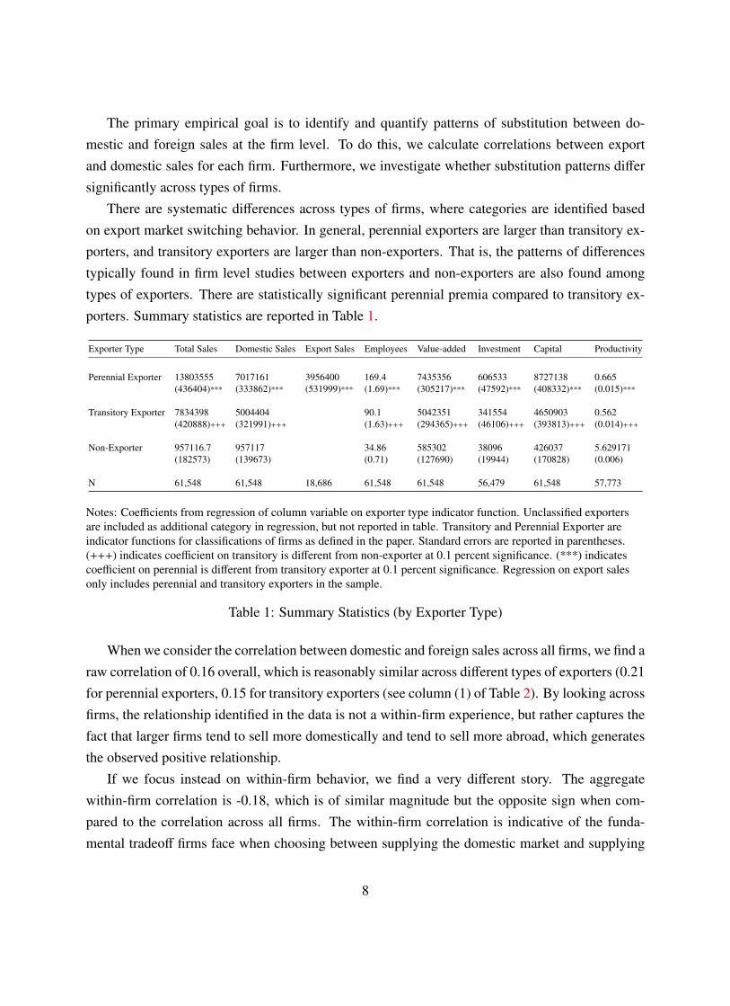
There are systematic differences across types of firms, where categories are identified basedon export market switching behavior. In general, perennial exporters are larger than transitory ex-porters, and transitory exporters are larger than non-exporters. That is, the patterns of differencestypically found in firm level studies between exporters and non-exporters are also found amongtypes of exporters. There are statistically significant perennial premia compared to transitory ex-porters. Summary statistics are reported in Table 1.

Exporter Type Total Sales Domestic Sales Export Sales Employees Value-added Investment Capital Productivity

Perennial Exporter 13803555 7017161 3956400 169.4 7435356 606533 8727138 0.665(436404)*** (333862)*** (531999)*** (1.69)*** (305217)*** (47592)*** (408332)*** (0.015)***

Transitory Exporter 7834398 5004404 90.1 5042351 341554 4650903 0.562(420888)+++ (321991)+++ (1.63)+++ (294365)+++ (46106)+++ (393813)+++ (0.014)+++

Non-Exporter 957116.7 957117 34.86 585302 38096 426037 5.629171(182573) (139673) (0.71) (127690) (19944) (170828) (0.006)

N 61,548 61,548 18,686 61,548 61,548 56,479 61,548 57,773

Notes: Coefficients from regression of column variable on exporter type indicator function. Unclassified exportersare included as additional category in regression, but not reported in table. Transitory and Perennial Exporter areindicator functions for classifications of firms as defined in the paper. Standard errors are reported in parentheses.(+++) indicates coefficient on transitory is different from non-exporter at 0.1 percent significance. (***) indicatescoefficient on perennial is different from transitory exporter at 0.1 percent significance. Regression on export salesonly includes perennial and transitory exporters in the sample.

Table 1: Summary Statistics (by Exporter Type)

When we consider the correlation between domestic and foreign sales across all firms, we find araw correlation of 0.16 overall, which is reasonably similar across different types of exporters (0.21for perennial exporters, 0.15 for transitory exporters (see column (1) of Table 2). By looking acrossfirms, the relationship identified in the data is not a within-firm experience, but rather captures thefact that larger firms tend to sell more domestically and tend to sell more abroad, which generatesthe observed positive relationship.

If we focus instead on within-firm behavior, we find a very different story. The aggregatewithin-firm correlation is -0.18, which is of similar magnitude but the opposite sign when com-pared to the correlation across all firms. The within-firm correlation is indicative of the funda-mental tradeoff firms face when choosing between supplying the domestic market and supplying

8

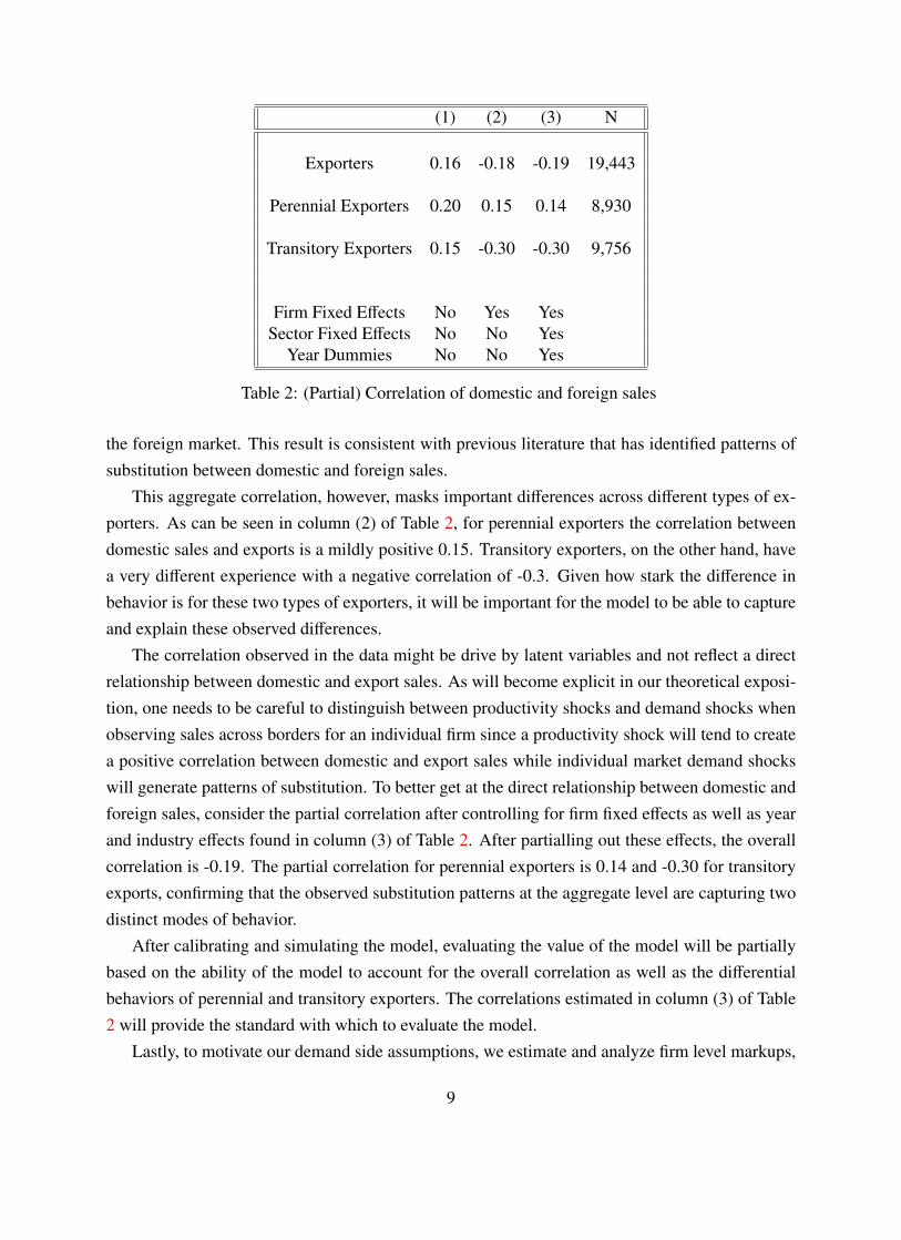
(1) (2) (3) N

Exporters 0.16 -0.18 -0.19 19,443

Perennial Exporters 0.20 0.15 0.14 8,930

Transitory Exporters 0.15 -0.30 -0.30 9,756

Firm Fixed Effects No Yes YesSector Fixed Effects No No Yes

Year Dummies No No Yes

Table 2: (Partial) Correlation of domestic and foreign sales

the foreign market. This result is consistent with previous literature that has identified patterns ofsubstitution between domestic and foreign sales.

This aggregate correlation, however, masks important differences across different types of ex-porters. As can be seen in column (2) of Table 2, for perennial exporters the correlation betweendomestic sales and exports is a mildly positive 0.15. Transitory exporters, on the other hand, havea very different experience with a negative correlation of -0.3. Given how stark the difference inbehavior is for these two types of exporters, it will be important for the model to be able to captureand explain these observed differences.

The correlation observed in the data might be drive by latent variables and not reflect a directrelationship between domestic and export sales. As will become explicit in our theoretical exposi-tion, one needs to be careful to distinguish between productivity shocks and demand shocks whenobserving sales across borders for an individual firm since a productivity shock will tend to createa positive correlation between domestic and export sales while individual market demand shockswill generate patterns of substitution. To better get at the direct relationship between domestic andforeign sales, consider the partial correlation after controlling for firm fixed effects as well as yearand industry effects found in column (3) of Table 2. After partialling out these effects, the overallcorrelation is -0.19. The partial correlation for perennial exporters is 0.14 and -0.30 for transitoryexports, confirming that the observed substitution patterns at the aggregate level are capturing twodistinct modes of behavior.

After calibrating and simulating the model, evaluating the value of the model will be partiallybased on the ability of the model to account for the overall correlation as well as the differentialbehaviors of perennial and transitory exporters. The correlations estimated in column (3) of Table2 will provide the standard with which to evaluate the model.

Lastly, to motivate our demand side assumptions, we estimate and analyze firm level markups,

9

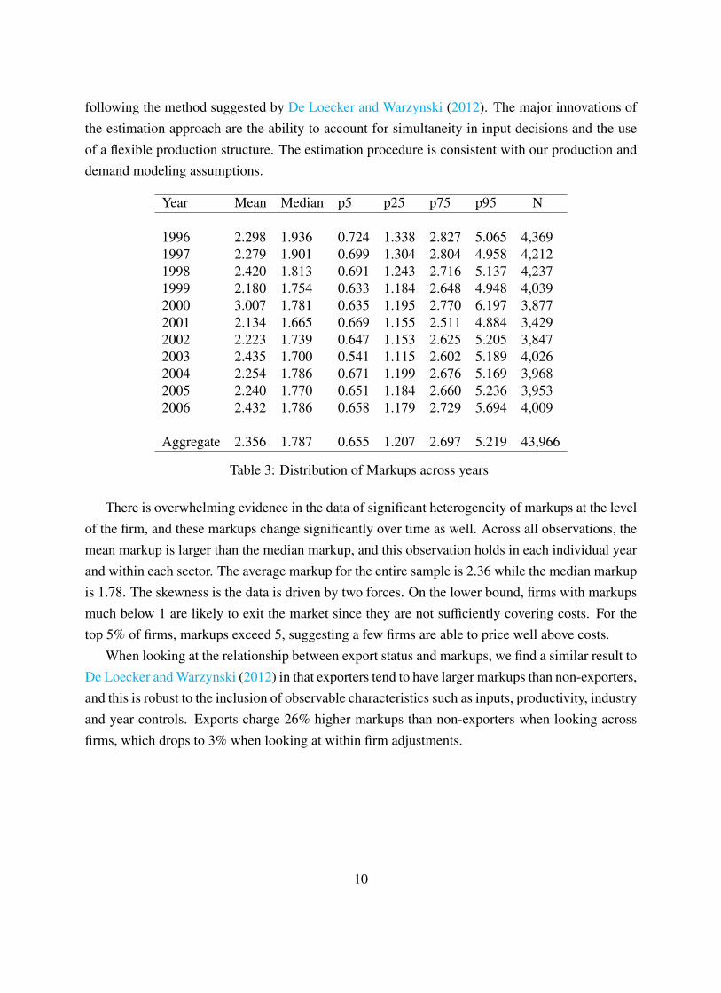
following the method suggested by De Loecker and Warzynski (2012). The major innovations ofthe estimation approach are the ability to account for simultaneity in input decisions and the useof a flexible production structure. The estimation procedure is consistent with our production anddemand modeling assumptions.

Year Mean Median p5 p25 p75 p95 N

1996 2.298 1.936 0.724 1.338 2.827 5.065 4,3691997 2.279 1.901 0.699 1.304 2.804 4.958 4,2121998 2.420 1.813 0.691 1.243 2.716 5.137 4,2371999 2.180 1.754 0.633 1.184 2.648 4.948 4,0392000 3.007 1.781 0.635 1.195 2.770 6.197 3,8772001 2.134 1.665 0.669 1.155 2.511 4.884 3,4292002 2.223 1.739 0.647 1.153 2.625 5.205 3,8472003 2.435 1.700 0.541 1.115 2.602 5.189 4,0262004 2.254 1.786 0.671 1.199 2.676 5.169 3,9682005 2.240 1.770 0.651 1.184 2.660 5.236 3,9532006 2.432 1.786 0.658 1.179 2.729 5.694 4,009

Aggregate 2.356 1.787 0.655 1.207 2.697 5.219 43,966

Table 3: Distribution of Markups across years

There is overwhelming evidence in the data of significant heterogeneity of markups at the levelof the firm, and these markups change significantly over time as well. Across all observations, themean markup is larger than the median markup, and this observation holds in each individual yearand within each sector. The average markup for the entire sample is 2.36 while the median markupis 1.78. The skewness is the data is driven by two forces. On the lower bound, firms with markupsmuch below 1 are likely to exit the market since they are not sufficiently covering costs. For thetop 5% of firms, markups exceed 5, suggesting a few firms are able to price well above costs.

When looking at the relationship between export status and markups, we find a similar result toDe Loecker and Warzynski (2012) in that exporters tend to have larger markups than non-exporters,and this is robust to the inclusion of observable characteristics such as inputs, productivity, industryand year controls. Exports charge 26% higher markups than non-exporters when looking acrossfirms, which drops to 3% when looking at within firm adjustments.

10

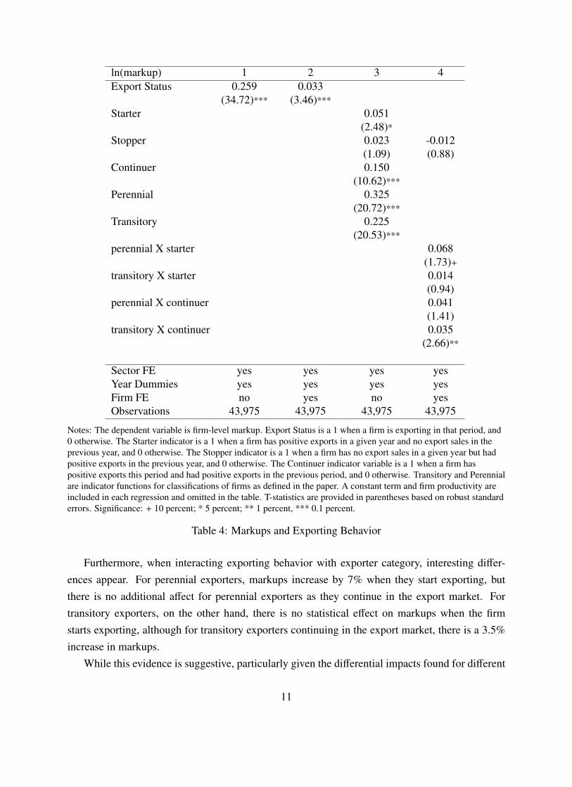
ln(markup) 1 2 3 4Export Status 0.259 0.033

(34.72)*** (3.46)***Starter 0.051

(2.48)*Stopper 0.023 -0.012

(1.09) (0.88)Continuer 0.150

(10.62)***Perennial 0.325

(20.72)***Transitory 0.225

(20.53)***perennial X starter 0.068

(1.73)+transitory X starter 0.014

(0.94)perennial X continuer 0.041

(1.41)transitory X continuer 0.035

(2.66)**

Sector FE yes yes yes yesYear Dummies yes yes yes yesFirm FE no yes no yesObservations 43,975 43,975 43,975 43,975

Notes: The dependent variable is firm-level markup. Export Status is a 1 when a firm is exporting in that period, and0 otherwise. The Starter indicator is a 1 when a firm has positive exports in a given year and no export sales in theprevious year, and 0 otherwise. The Stopper indicator is a 1 when a firm has no export sales in a given year but hadpositive exports in the previous year, and 0 otherwise. The Continuer indicator variable is a 1 when a firm haspositive exports this period and had positive exports in the previous period, and 0 otherwise. Transitory and Perennialare indicator functions for classifications of firms as defined in the paper. A constant term and firm productivity areincluded in each regression and omitted in the table. T-statistics are provided in parentheses based on robust standarderrors. Significance: + 10 percent; * 5 percent; ** 1 percent, *** 0.1 percent.

Table 4: Markups and Exporting Behavior

Furthermore, when interacting exporting behavior with exporter category, interesting differ-ences appear. For perennial exporters, markups increase by 7% when they start exporting, butthere is no additional affect for perennial exporters as they continue in the export market. Fortransitory exporters, on the other hand, there is no statistical effect on markups when the firmstarts exporting, although for transitory exporters continuing in the export market, there is a 3.5%increase in markups.

While this evidence is suggestive, particularly given the differential impacts found for different

11

types of exporters, since exporting behavior is not randomly assigned, there should be caution ininterpreting these results causally. We will return to these issues when we conduct counterfactualexperiments on the simulated data. We now turn to building the theoretical model with these factsand relationships in mind.

3 Model

Guided by the evidence presented in the previous section, we drop the traditional assumptionsof sunk and fixed costs to entry in the export market and constant marginal costs of production.The existence of two groups of exporters in the data, one that is perennially in the export marketand one that regularly cycles in and out of the export market along with no observed discrete jumpin total sales when a firm enters (or exits) suggests the assumption of sunk and fixed costs ofexporting may be inappropriate. Furthermore, the patterns of substitution between domestic andforeign sales observed is inconsistent with a constant marginal cost assumption.

We address these empirical regularities by extending the Melitz-Ottaviano linear demand sys-tem with non-constant elasticity of firm demand to include increasing marginal cost to productionand three distinct firm shocks (shock to productivity, domestic demand, and export demand). Thelinear demand system generates a choke price above which demand is zero, and drops the assump-tion of fixed costs to rationalize the fact that few firms export. Increasing marginal cost gives riseto the observed patterns of substation between domestic and foreign sales.

Time runs t = 0, 1, . . . . There are two symmetric countries, populated by a continuum ofconsumers of mass 1. Country H is the Home country and country F is the foreign country.

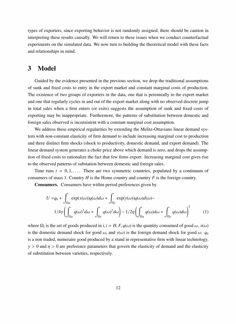
Consumers. Consumers have within period preferences given by

U =q0 +

∫ΩH

exp(x(ω))q(ω)dω +

∫ΩF

exp(y(ω))q(ω)d(ω)−

1/4γ(∫

ΩH

q(ω)2dω +

∫ΩF

q(ω)2dω)− 1/2η

(∫ΩH

q(ω)dω +

∫ΩF

q(ω)dω)2

(1)

where Ωi is the set of goods produced in i, i = H, F, q(ω) is the quantity consumed of good ω, x(ω)is the domestic demand shock for good ω, and y(ω) is the foreign demand shock for good ω. q0

is a non traded, numeraire good produced by a stand in representative firm with linear technology.γ > 0 and η > 0 are preference parameters that govern the elasticity of demand and the elasticityof substitution between varieties, respectively.

12

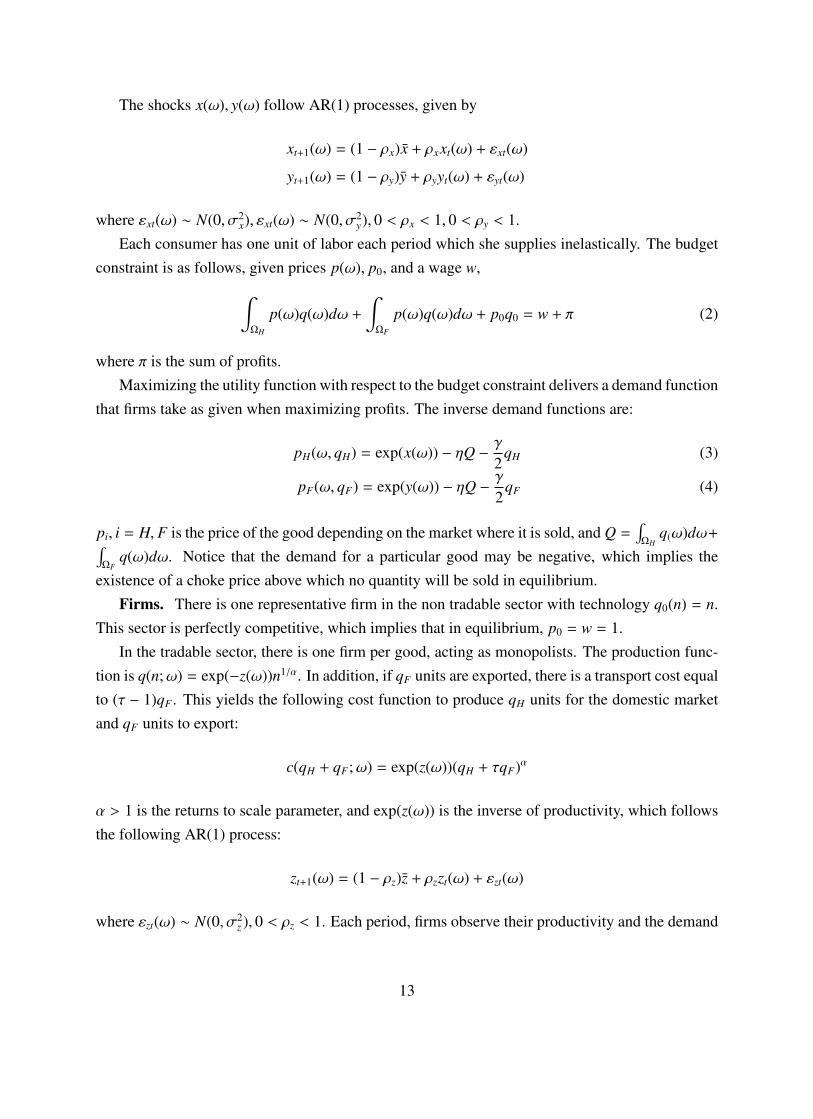
The shocks x(ω), y(ω) follow AR(1) processes, given by

xt+1(ω) = (1 − ρx)x + ρxxt(ω) + εxt(ω)

yt+1(ω) = (1 − ρy)y + ρyyt(ω) + εyt(ω)

where εxt(ω) ∼ N(0, σ2x), εxt(ω) ∼ N(0, σ2

y), 0 < ρx < 1, 0 < ρy < 1.Each consumer has one unit of labor each period which she supplies inelastically. The budget

constraint is as follows, given prices p(ω), p0, and a wage w,∫ΩH

p(ω)q(ω)dω +

∫ΩF

p(ω)q(ω)dω + p0q0 = w + π (2)

where π is the sum of profits.Maximizing the utility function with respect to the budget constraint delivers a demand function

that firms take as given when maximizing profits. The inverse demand functions are:

pH(ω, qH) = exp(x(ω)) − ηQ −γ

2qH (3)

pF(ω, qF) = exp(y(ω)) − ηQ −γ

2qF (4)

pi, i = H, F is the price of the good depending on the market where it is sold, and Q =∫

ΩHq(ω)dω+∫

ΩFq(ω)dω. Notice that the demand for a particular good may be negative, which implies the

existence of a choke price above which no quantity will be sold in equilibrium.Firms. There is one representative firm in the non tradable sector with technology q0(n) = n.

This sector is perfectly competitive, which implies that in equilibrium, p0 = w = 1.In the tradable sector, there is one firm per good, acting as monopolists. The production func-

tion is q(n;ω) = exp(−z(ω))n1/α. In addition, if qF units are exported, there is a transport cost equalto (τ − 1)qF . This yields the following cost function to produce qH units for the domestic marketand qF units to export:

c(qH + qF;ω) = exp(z(ω))(qH + τqF)α

α > 1 is the returns to scale parameter, and exp(z(ω)) is the inverse of productivity, which followsthe following AR(1) process:

zt+1(ω) = (1 − ρz)z + ρzzt(ω) + εzt(ω)

where εzt(ω) ∼ N(0, σ2z ), 0 < ρz < 1. Each period, firms observe their productivity and the demand

13

shocks and choose prices and quantities to maximize profits. That is, firm ω solves

maxpH ,qH ,pF ,qF

pHqH + pFqF − exp(z(ω))(qH + τqF)α (5)

s.t. equations (3) and (4).

Market Clearing. In equilibrium, all firms producing tradable goods with positive demands(x > ηQ or y > ηQ) will demand labor units. The representative firm producing non tradable goodsalso demands labor. The quasilinear nature of preferences implies that all labor in excess of thatdemanded by the tradable sector is absorbed by the non tradable sector. Thus,

∫ΩH

n(ω)dω+n0 = 1,where n(ω) solves problem (5) and n0 is the labor demand of the non tradable sector.

3.1 Equilibrium

While the setup is dynamic, the decisions of the firm are static, since there is no endogenousstate variable. Also, we have not introduced any elements to transfer resources intertemporally,such as bonds. Notice that introducing bonds would not matter because of the assumption ofsymmetric consumers and symmetric countries. Thus, we can define a static equilibrium as a listof quantities q(ω) and q0, labor inputs n(ω) and n0 and prices p(ω) such that consumers maximize(1) subject to equation (2), firms solve (5), and markets clear.

In what follows, it is convenient to drop the name of the good ω and refer to firms accordingto their type. Each firm is a triplet (x, y, z). In equilibrium, the solution to problem (5) allows forseveral corners. In particular, when exp(x) < ηQ, the good will not be sold domestically, and whenexp(y) < ηQ, it will not be exported. Still, when neither of these conditions are met, it will besometimes optimal to sell in only one market. The next proposition shows all the possible cases.

Proposition 1. A firm x, y, z will only sell domestically when exp(x) > ηQ and x > x(y, z). Sim-

ilarly, it will only export when exp(y) > ηQ and y > y(x, z). It will sell in both markets when

exp(x) > ηQ, exp(y) > ηQ, x ≥ y(x, z) and y ≥ y(x, z), where

x(y, z) = log

γ (exp(y) − ηQτα exp(z)

) 1α−1

+exp(y) − ηQ

τ+ ηQ

(6)

y(x, z) = log

γτ(exp(x) − ηQα exp(z)

) 1α−1

+ τ(exp(x) − ηQ

)+ ηQ

(7)

Proof. The proof is straightforward, and detailed in the Appendix. Intuitively, when x is too largerelative to y, the firm will choose not to export, since exporting increases its marginal cost givendecreasing returns to scale, may be optimal to keep these costs low. The opposite happens if y is

14

large relative to x, in which case the firm will choose not to sell domestically and export all itsoutput.

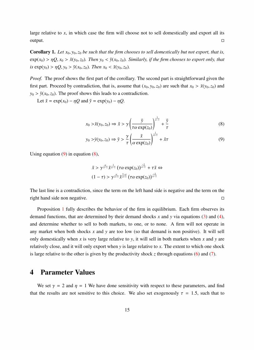
Corollary 1. Let x0, y0, z0 be such that the firm chooses to sell domestically but not export, that is,

exp(x0) > ηQ, x0 > x(y0, z0). Then y0 < y(x0, z0). Similarly, if the firm chooses to export only, that

is exp(y0) > ηQ, y0 > y(x0, z0). Then x0 < x(y0, z0).

Proof. The proof shows the first part of the corollary. The second part is straightforward given thefirst part. Proceed by contradiction, that is, assume that (x0, y0, z0) are such that x0 > x(y0, z0) andy0 > y(x0, z0). The proof shows this leads to a contradiction.

Let x = exp(x0) − ηQ and y = exp(y0) − ηQ.

x0 >x(y0, z0)⇒ x > γ(

yτα exp(z0)

) 1α−1

+yτ

(8)

y0 >y(y0, z0)⇒ y >γ

τ

(x

α exp(z0)

) 1α−1

+ xτ (9)

Using equation (9) in equation (8),

x > γαα−1 x

1α−1

(τα exp(z0)

) −2α−1 + τx⇔

(1 − τ) > γαα−1 x

2−αα−1

(τα exp(z0)

) −2α−1

The last line is a contradiction, since the term on the left hand side is negative and the term on theright hand side non negative.

Proposition 1 fully describes the behavior of the firm in equilibrium. Each firm observes itsdemand functions, that are determined by their demand shocks x and y via equations (3) and (4),and determine whether to sell to both markets, to one, or to none. A firm will not operate inany market when both shocks x and y are too low (so that demand is non positive). It will sellonly domestically when x is very large relative to y, it will sell in both markets when x and y arerelatively close, and it will only export when y is large relative to x. The extent to which one shockis large relative to the other is given by the productivity shock z through equations (6) and (7).

4 Parameter Values

We set γ = 2 and η = 1 We have done sensitivity with respect to these parameters, and findthat the results are not sensitive to this choice. We also set exogenously τ = 1.5, such that to

15

export one unit, the exporter must produce 1.5. Sensitivity experiments show that results do notdepend critically on this parameter, which at first seems important given that this is a key tradeparameter. The reason is that increases in τ are associated with similar increases in y or in σy,which counteract the initial effect of τ. In other words, we were unable to successfully identify theeffect of τ from the effect of y or σy.

For the parameters governing the distribution of firms we use firm level data on domestic rev-enues, exports and mark-ups to back out the unobserved triplet (x, y, z) consistent with the observeddata.8 This procedure assumes that we know the value of Q. Fortunately, the free parameter M

determines Q. So we set Q = 1 and back out the M that is consistent with this equilibrium value.We do this for all firms in year 1996.9

The model implies that, as t → ∞, the economy converges to an invariant distribution offirms operating. Given the autorregressive nature of the stochastic processes, the unconditionaldistributions of the shocks are

x ∼ N(x,

σ2x

1 − ρ2x

), y ∼ N

y, σ2y

1 − ρ2y

, z ∼ N(z,

σ2z

1 − ρ2z

)This distribution, paired with the optimizing strategies x(y, z) and the invariant distributions, implyan invariant distribution for quantities and sales.

We observe an unbiased sample of productivities z, so we can structurally estimate the param-eters z and σz =

σ2z

1−ρ2z

via maximum likelihood. We pick α = 1.5, which implies that the labor sharein the production function is 2/3. This is somewhat larger that the returns estimated by Cosar et al.(2010), which is 1.66. However, Hopenhayn and Rogerson (1993) and others use a lower number,closer to 1.2. Thus, we set α = 1.5.

For the demand parameters, we only observe a biased sample. For example, if the firm onlysells domestically, we observe x but not y. Moreover, we know x > ηQ and x > x(y, z), so y

must satisfy this condition. A similar argument holds for firms that choose to export but not selldomestically (we do not observe x in this case). However, there are very few cases in which thefirm only exports (3 firms out of 1,417 export only among the firms operating every period). Thus,we eliminate these observations and assume that we observe all x such that x > ηQ. Moreover,our backed out values for x suggest that the condition x > ηQ is rarely binding. Accordingly, weignore it and estimate the parameters x and σx =

σ2x

1−ρ2x

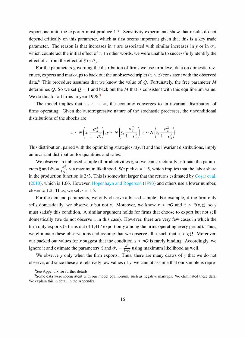
using maximum likelihood as well.We observe y only when the firm exports. Thus, there are many draws of y that we do not

observe, and since these are relatively low values of y, we cannot assume that our sample is repre-

8See Appendix for further details.9Some data were inconsistent with our model equilibrium, such as negative markups. We eliminated these data.

We explain this in detail in the Appendix.

16

sentative, which prevents us from estimating the relevant parameters via MLE. Alternatively, thedistribution for y is key to determine exports, so we calibrate y and σy such that the ratio of exportsto total sales and the share of exporters is as in the data (30% and 32% respectively).10

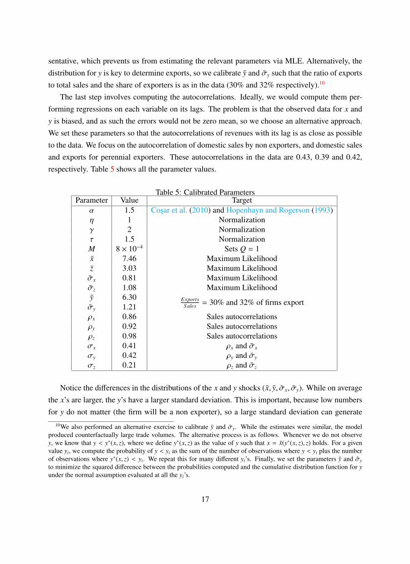
The last step involves computing the autocorrelations. Ideally, we would compute them per-forming regressions on each variable on its lags. The problem is that the observed data for x andy is biased, and as such the errors would not be zero mean, so we choose an alternative approach.We set these parameters so that the autocorrelations of revenues with its lag is as close as possibleto the data. We focus on the autocorrelation of domestic sales by non exporters, and domestic salesand exports for perennial exporters. These autocorrelations in the data are 0.43, 0.39 and 0.42,respectively. Table 5 shows all the parameter values.

Table 5: Calibrated ParametersParameter Value Target

α 1.5 Cosar et al. (2010) and Hopenhayn and Rogerson (1993)η 1 Normalizationγ 2 Normalizationτ 1.5 NormalizationM 8 × 10−4 Sets Q = 1x 7.46 Maximum Likelihoodz 3.03 Maximum Likelihoodσx 0.81 Maximum Likelihoodσz 1.08 Maximum Likelihoody 6.30 Exports

S ales = 30% and 32% of firms exportσy 1.21ρx 0.86 Sales autocorrelationsρy 0.92 Sales autocorrelationsρz 0.98 Sales autocorrelationsσx 0.41 ρx and σx

σy 0.42 ρy and σy

σz 0.21 ρz and σz

Notice the differences in the distributions of the x and y shocks (x, y, σx, σy). While on averagethe x’s are larger, the y’s have a larger standard deviation. This is important, because low numbersfor y do not matter (the firm will be a non exporter), so a large standard deviation can generate

10We also performed an alternative exercise to calibrate y and σy. While the estimates were similar, the modelproduced counterfactually large trade volumes. The alternative process is as follows. Whenever we do not observey, we know that y < y∗(x, z), where we define y∗(x, z) as the value of y such that x = x(y∗(x, z), z) holds. For a givenvalue yi, we compute the probability of y < yi as the sum of the number of observations where y < yi plus the numberof observations where y∗(x, z) < yi. We repeat this for many different yi’s. Finally, we set the parameters y and σy

to minimize the squared difference between the probabilities computed and the cumulative distribution function for yunder the normal assumption evaluated at all the yi’s.

17

large trade volumes in spite of small means. In this case, both the trade volume of 30 percent andthe fact that 32 percent of firms export within a given year imply x > y and σx < σy.

5 Findings

5.1 Exports and Domestic Sales

The main question in the paper is whether the model can account for the correlations betweendomestic and foreign sales in the data. This correlation is -0.19 across the board. Dividing the sam-ple between type of exporters, the correlation for transitory exporters is -0.30, and the correlationfor perennial exporters is 0.14.

In the model, the overall correlation is -0.15. It is -0.19 for transitory exporters, and 0.02 forpermanent exporters. Thus, the model can account fairly reasonably for the change in sign betweenperennial and transitory exporters. Quantitatively, it accounts for almost 80 percent of the overallcorrelation. However, this is not evenly split among the subgroups: while it accounts for two thirdsof the negative correlation among transitory exporters, it only accounts for 14 percent in the caseof perennial exporters.

Next we try to understand why the correlation for transitory exporters is so much lower thanfor perennial exporters. We conjecture that this is due to the shape of the cost curve. Marginalcosts are exp(z)αQα−1, where Q is units produced. Since 1 < α < 2, this function is increasing andconcave, so that marginal costs increase at a decreasing rate. Thus, marginal costs are relativelyflatter (closer to constant returns) for larger firms. If this is the reason for the lower correlationamong transitory exporters, then we should expect transitory exporters to be relatively smaller thanperennial exporters. We verify this by performing the following regression on all firms, includingnon-exporters:

log(Qit) = β0 + β1IPi + β2ITi + εit

where

IPi =

1 if firm i is a perennial exporter

0 otherwiseand ITi =

1 if firm i is a transitory exporter

0 otherwise

Our estimates confirm that perennial exporters are on average larger than transitory exporters,which are on average larger than non exporters. The estimates are β1 = 1.42 and β2 = 0.62. Thisimplies that, on average, perennial exporters produce 140 percent more than non exporters, andtransitory exporters produce 62 percent more than non exporters, confirming our conjecture that

18

perennial exporters are on average larger than non exporters. These estimates are significant at the1 percent level. If we replace physical quantities with sales, we still get the same effect, and theestimates suggest that perennial exporters sell 92 percent more than non exporters, while transitoryexporters sell 30 percent more.

We then explore the effect of exports on the domestic price charged by a firm. To do this, weregress the (log of) the difference in price charged by a firm on a dummy indicating whether afirm started or stopped exporting. We first simulate the behavior of 10,000 firms for 1,000 periods,of which we only keep the last 10. We keep only firms that exported in some but not all thelast 10 periods (and sold domestically in all 10 periods). Then we compute the difference in thedomestic price between any 2 consecutive periods (pt+1/pt), and regress this measure against twodummies indicating whether the firm started or stopped exporting in that period. We control forthe difference in productivity shocks and both demand shocks. That is, we perform the followingregression using simulated data:

log(

pid,t

pid,t−1

)= β0 + β1Enteri,t + β2Exiti,t+

β3(xi,t − xi,t−1) + β4(yi,t − yi,t−1) + β5(zi,t − zi,t−1) + εi,t

We are interested in the coefficients β1 and β2. We find that β1 = 0.008 and β2 = −0.008, significantat the 1% level. Thus, starting to export increases the domestic price by 0.8 percent, and exiting theexport market reduces it by the same amount. Starting to export increases the quantity produced,increasing the marginal cost, and subsequently the price.

5.2 Counterfactuals

To learn more about the interaction between exports and domestic sales, we drop trade costsfrom our benchmark value of 1.5 to 1.1.

Sales

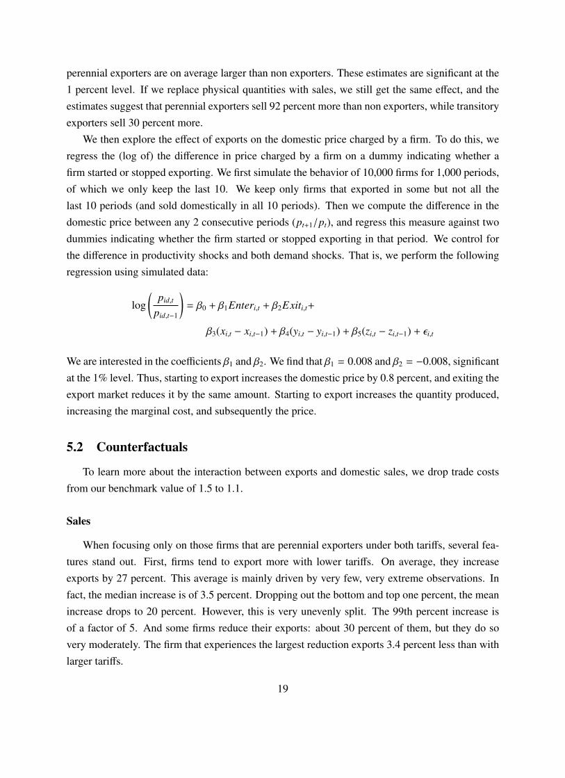
When focusing only on those firms that are perennial exporters under both tariffs, several fea-tures stand out. First, firms tend to export more with lower tariffs. On average, they increaseexports by 27 percent. This average is mainly driven by very few, very extreme observations. Infact, the median increase is of 3.5 percent. Dropping out the bottom and top one percent, the meanincrease drops to 20 percent. However, this is very unevenly split. The 99th percent increase isof a factor of 5. And some firms reduce their exports: about 30 percent of them, but they do sovery moderately. The firm that experiences the largest reduction exports 3.4 percent less than withlarger tariffs.

19

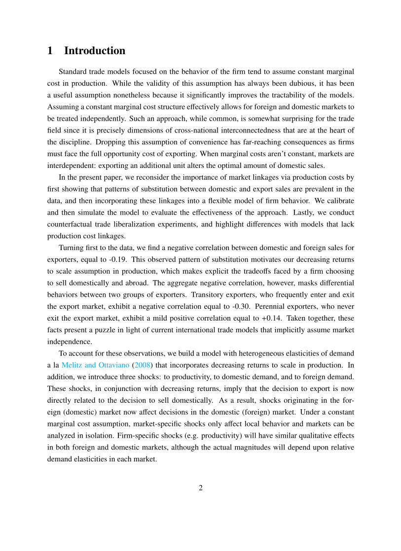
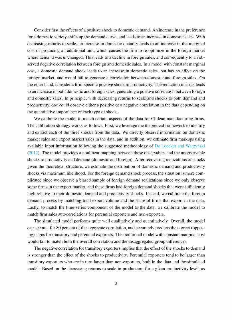
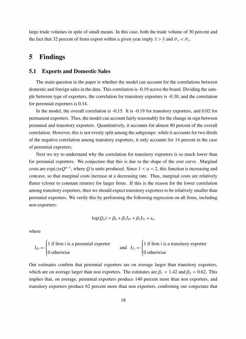
Exporters also tend to increase their domestic sales when trade costs fall. The mean increaseis almost 7 percent, while the median increase is zero. About 50 percent of firms increase theirdomestic sales volume. Figures 1 and 2 show the distribution of increases in domestic and foreignsales.11

0.96 0.98 1 1.02 1.04 1.06 1.08 1.1 1.120

0.1

0.2

0.3

0.4

0.5

0.6

0.7

Figure 1: Increase in Domestic Sales by Perennial Exporters when Trade Barriers Drop

The facts that some firms sell more domestically after a reduction in tariffs is not present instandard international trade models. In our model, the reason for this is as follows. A reductionin trade costs implies a gain in efficiency and a reduction in costs. While this affects exports morethan domestic sales, the decreasing returns to scale technology implies that cost reductions are alsopresent for domestic output. When faced with a reduction in costs, firms tend to increase output.Which part of output increases the most depends on the elasticities of demand. In fact, we ask themodel how the elasticities affect the change in revenues. To do this, we perform two regressions.The first regresses the increase in domestic sales (in logs) against the difference in the domesticand foreign elasticity of demand. The second regression does the same changing the dependentvariable for the increase in exports. That is, we regress

log(

Domestic sales low τ

Domestic sales high τ

)= β0d + β1d(|ηd| − |ηx|) + εd

log(

Exports low τ

Exports high τ

)= β0x + β1x(|ηd| − |ηx|) + εx

11For expositional purposes, this does not include the top and bottom 1 percent.

20

1 1.2 1.4 1.6 1.8 2 2.20

0.05

0.1

0.15

0.2

0.25

0.3

0.35

0.4

Figure 2: Increase in Exports by Perennial Exporters when Trade Barriers Drop

where ηd is domestic and ηx is foreign elasticity of demand, defined as

ηd =∂qd

∂pd

pd

qd= −

ex − ηQ − γ/2qd

γ/2qd

ηx =∂qx

∂px

px

qx= −

ey − ηQ − γ/2qx

γ/2qx

We evaluate the quantities qd, qx and Q at the average before and after the drop in τ. Table 6 showsour results. The estimates are very robust, and confirm that when the domestic demand is moreelastic than the foreign demand, the reduction in costs (and prices), leads to larger increases indomestic sales. When the opposite happens, foreign demand increases more.

Parameter Estimate p-value R2

β1d 0.0286 0.0000 0.6776β1x -0.0350 0.0000 0.2241

Table 6: Elasticities and the change in domestic and foreign sales

Notice that the key elements for these results are decreasing returns to scale technologies, andheterogeneous elasticities of demand. Models based on Dixit-Stiglitz preferences cannot replicatethis, even when paired with decreasing returns to scale technologies. In fact, in Melitz (2003), do-mestic sales can only be affected via a general equilibrium effect (wages increase after a reductionin trade costs), and unequivocally domestic sales drop in this case.

21

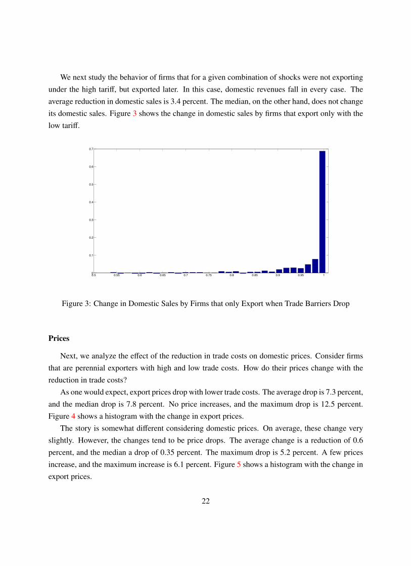
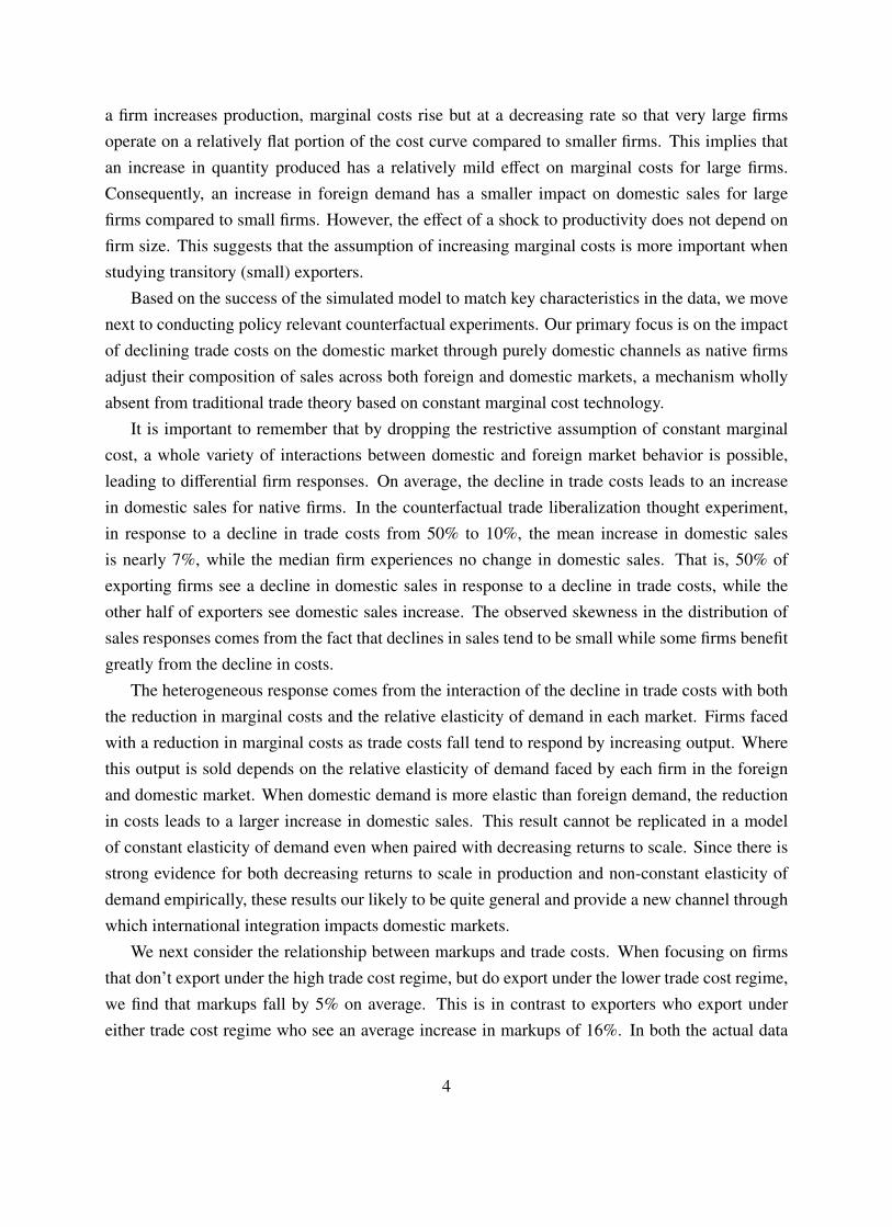
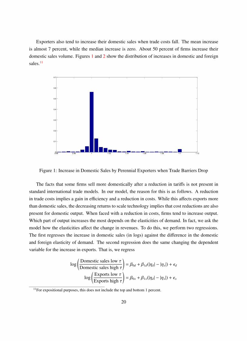
We next study the behavior of firms that for a given combination of shocks were not exportingunder the high tariff, but exported later. In this case, domestic revenues fall in every case. Theaverage reduction in domestic sales is 3.4 percent. The median, on the other hand, does not changeits domestic sales. Figure 3 shows the change in domestic sales by firms that export only with thelow tariff.

0.5 0.55 0.6 0.65 0.7 0.75 0.8 0.85 0.9 0.95 10

0.1

0.2

0.3

0.4

0.5

0.6

0.7

Figure 3: Change in Domestic Sales by Firms that only Export when Trade Barriers Drop

Prices

Next, we analyze the effect of the reduction in trade costs on domestic prices. Consider firmsthat are perennial exporters with high and low trade costs. How do their prices change with thereduction in trade costs?

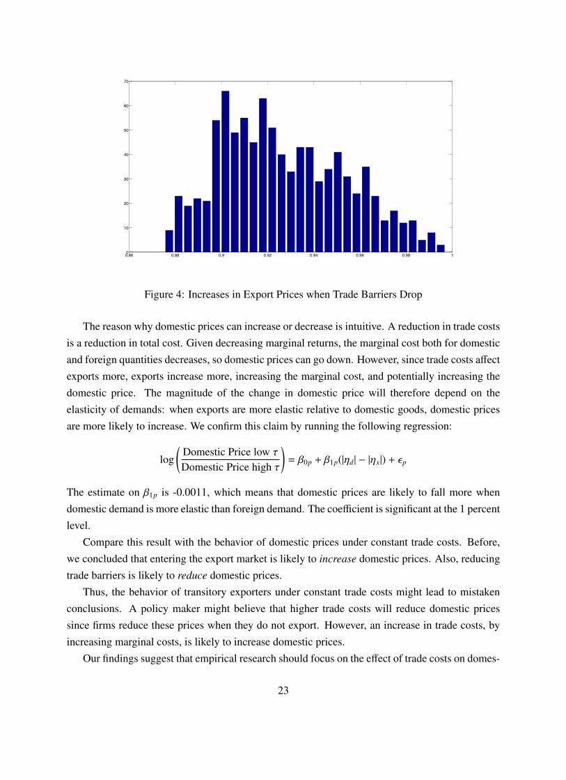
As one would expect, export prices drop with lower trade costs. The average drop is 7.3 percent,and the median drop is 7.8 percent. No price increases, and the maximum drop is 12.5 percent.Figure 4 shows a histogram with the change in export prices.

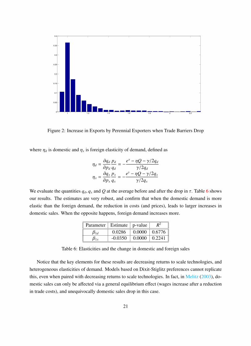
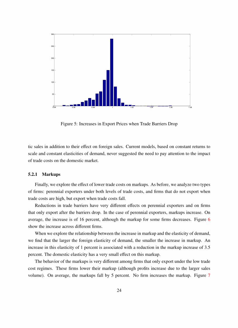
The story is somewhat different considering domestic prices. On average, these change veryslightly. However, the changes tend to be price drops. The average change is a reduction of 0.6percent, and the median a drop of 0.35 percent. The maximum drop is 5.2 percent. A few pricesincrease, and the maximum increase is 6.1 percent. Figure 5 shows a histogram with the change inexport prices.

22

0.86 0.88 0.9 0.92 0.94 0.96 0.98 10

10

20

30

40

50

60

70

Figure 4: Increases in Export Prices when Trade Barriers Drop

The reason why domestic prices can increase or decrease is intuitive. A reduction in trade costsis a reduction in total cost. Given decreasing marginal returns, the marginal cost both for domesticand foreign quantities decreases, so domestic prices can go down. However, since trade costs affectexports more, exports increase more, increasing the marginal cost, and potentially increasing thedomestic price. The magnitude of the change in domestic price will therefore depend on theelasticity of demands: when exports are more elastic relative to domestic goods, domestic pricesare more likely to increase. We confirm this claim by running the following regression:

log(

Domestic Price low τ

Domestic Price high τ

)= β0p + β1p(|ηd| − |ηx|) + εp

The estimate on β1p is -0.0011, which means that domestic prices are likely to fall more whendomestic demand is more elastic than foreign demand. The coefficient is significant at the 1 percentlevel.

Compare this result with the behavior of domestic prices under constant trade costs. Before,we concluded that entering the export market is likely to increase domestic prices. Also, reducingtrade barriers is likely to reduce domestic prices.

Thus, the behavior of transitory exporters under constant trade costs might lead to mistakenconclusions. A policy maker might believe that higher trade costs will reduce domestic pricessince firms reduce these prices when they do not export. However, an increase in trade costs, byincreasing marginal costs, is likely to increase domestic prices.

Our findings suggest that empirical research should focus on the effect of trade costs on domes-

23

0.94 0.96 0.98 1 1.02 1.04 1.06 1.080

50

100

150

200

250

300

Figure 5: Increases in Export Prices when Trade Barriers Drop

tic sales in addition to their effect on foreign sales. Current models, based on constant returns toscale and constant elasticities of demand, never suggested the need to pay attention to the impactof trade costs on the domestic market.

5.2.1 Markups

Finally, we explore the effect of lower trade costs on markups. As before, we analyze two typesof firms: perennial exporters under both levels of trade costs, and firms that do not export whentrade costs are high, but export when trade costs fall.

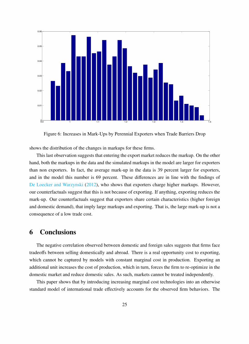
Reductions in trade barriers have very different effects on perennial exporters and on firmsthat only export after the barriers drop. In the case of perennial exporters, markups increase. Onaverage, the increase is of 16 percent, although the markup for some firms decreases. Figure 6show the increase across different firms.

When we explore the relationship between the increase in markup and the elasticity of demand,we find that the larger the foreign elasticity of demand, the smaller the increase in markup. Anincrease in this elasticity of 1 percent is associated with a reduction in the markup increase of 3.5percent. The domestic elasticity has a very small effect on this markup.

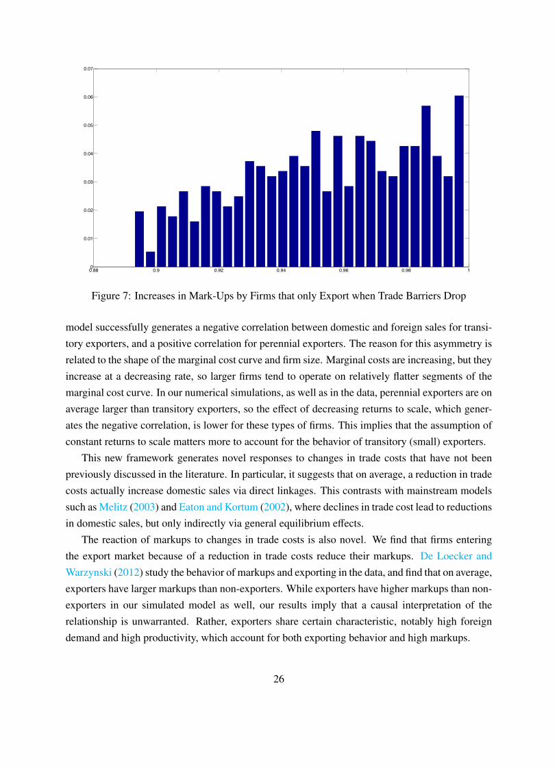
The behavior of the markups is very different among firms that only export under the low tradecost regimes. These firms lower their markup (although profits increase due to the larger salesvolume). On average, the markups fall by 5 percent. No firm increases the markup. Figure 7

24

0.9 1 1.1 1.2 1.3 1.4 1.50

0.01

0.02

0.03

0.04

0.05

0.06

Figure 6: Increases in Mark-Ups by Perennial Exporters when Trade Barriers Drop

shows the distribution of the changes in markups for these firms.This last observation suggests that entering the export market reduces the markup. On the other

hand, both the markups in the data and the simulated markups in the model are larger for exportersthan non exporters. In fact, the average mark-up in the data is 39 percent larger for exporters,and in the model this number is 69 percent. These differences are in line with the findings ofDe Loecker and Warzynski (2012), who shows that exporters charge higher markups. However,our counterfactuals suggest that this is not because of exporting. If anything, exporting reduces themark-up. Our counterfactuals suggest that exporters share certain characteristics (higher foreignand domestic demand), that imply large markups and exporting. That is, the large mark-up is not aconsequence of a low trade cost.

6 Conclusions

The negative correlation observed between domestic and foreign sales suggests that firms facetradeoffs between selling domestically and abroad. There is a real opportunity cost to exporting,which cannot be captured by models with constant marginal cost in production. Exporting anadditional unit increases the cost of production, which in turn, forces the firm to re-optimize in thedomestic market and reduce domestic sales. As such, markets cannot be treated independently.

This paper shows that by introducing increasing marginal cost technologies into an otherwisestandard model of international trade effectively accounts for the observed firm behaviors. The

25

0.88 0.9 0.92 0.94 0.96 0.98 10

0.01

0.02

0.03

0.04

0.05

0.06

0.07

Figure 7: Increases in Mark-Ups by Firms that only Export when Trade Barriers Drop

model successfully generates a negative correlation between domestic and foreign sales for transi-tory exporters, and a positive correlation for perennial exporters. The reason for this asymmetry isrelated to the shape of the marginal cost curve and firm size. Marginal costs are increasing, but theyincrease at a decreasing rate, so larger firms tend to operate on relatively flatter segments of themarginal cost curve. In our numerical simulations, as well as in the data, perennial exporters are onaverage larger than transitory exporters, so the effect of decreasing returns to scale, which gener-ates the negative correlation, is lower for these types of firms. This implies that the assumption ofconstant returns to scale matters more to account for the behavior of transitory (small) exporters.

This new framework generates novel responses to changes in trade costs that have not beenpreviously discussed in the literature. In particular, it suggests that on average, a reduction in tradecosts actually increase domestic sales via direct linkages. This contrasts with mainstream modelssuch as Melitz (2003) and Eaton and Kortum (2002), where declines in trade cost lead to reductionsin domestic sales, but only indirectly via general equilibrium effects.

The reaction of markups to changes in trade costs is also novel. We find that firms enteringthe export market because of a reduction in trade costs reduce their markups. De Loecker andWarzynski (2012) study the behavior of markups and exporting in the data, and find that on average,exporters have larger markups than non-exporters. While exporters have higher markups than non-exporters in our simulated model as well, our results imply that a causal interpretation of therelationship is unwarranted. Rather, exporters share certain characteristic, notably high foreigndemand and high productivity, which account for both exporting behavior and high markups.

26

A particularly appealing aspect of the approach taken here is that a simple, tractable modelcan account for relevant correlations in the data. Alternative approaches based on physical andfinancial capacity constraints could be reconciled with transitory and perennial exporter behaviors,but would require a more complicated approach that incorporates dynamic investment in capacitywith nonlinear costs and uncertainty. The results presented here show that such complications arenot necessary for matching observed patterns. The flexibility and efficiency of the present modelis a virtue in this regard.

Our results suggest that future research on international trade should consider frameworks withnon-constant returns to scale. This implies that firm decisions on exports and domestic sales cannotbe considered in isolation, and shocks to one market will have effects on both markets. In particular,the need for decreasing marginal returns is especially important to understand the high frequencyresponse to shocks of relatively small exporters.

27

References

Ahn, JaeBin and Alexander McQuoid, “Capacity constrained exporters: micro evidence andmacro implications,” 2013.

Almeida, Rita and Ana M. Fernandes, “Explaining local manufacturing growth in Chile: theadvantages of sectoral diversity,” Applied Economics, June 2013, 45 (16), 2201–2213.

Arkolakis, Costas, Jonathan Eaton, and Samuel Kortum, “Staggered Adjustment and TradeDynamics,” November 2011.

Atkeson, Andrew and Ariel Tomas Burstein, “Innovation, Firm Dynamics, and InternationalTrade,” Journal of Political Economy, 06 2010, 118 (3), 433–484.

Berman, Nicolas, Antoine Berthou, and Jerome Hericourt, “Export Dynamics and Sales atHome,” August 2011.

Blum, Bernardo, Sebastain Claro, and Ignatius Horstmann, “Occasional vs Perennial Ex-porters: The Impact of Capacity on Export Mode,” Journal of International Economics, May2013, 90, 1, 65–74.

Cosar, A Kerem, Nezih Guner, and James Tybout, “Firm dynamics, job turnover, and wagedistributions in an open economy,” Technical Report, National Bureau of Economic Research2010.

Eaton, Jonathan and Samuel Kortum, “Technology, Geography, and Trade,” Econometrica,September 2002, 70 (5), 1741–1779.

Hopenhayn, Hugo and Richard Rogerson, “Job turnover and policy evaluation: A general equi-librium analysis,” Journal of political Economy, 1993, pp. 915–938.

Kohn, David, Fernando Leibovici, and Michal Szkup, “Financial Frictions and New ExporterDynamics,” January 2012.

Liu, Lili, “Entry-exit, learning, and productivity change Evidence from Chile,” Journal of Devel-

opment Economics, 1993, 42 (2), 217 – 242.

Loecker, Jan De and Frederic Warzynski, “Markups and Firm-Level Export Status,” American

Economic Review, May 2012, 102 (6), 2437–71.

Melitz, Marc J., “The Impact of Trade on Intra-Industry Reallocations and Aggregate IndustryProductivity,” Econometrica, 2003, 71 (6), pp. 1695–1725.

28

Melitz, Marc J and Gianmarco IP Ottaviano, “Market size, trade, and productivity,” The review

of economic studies, 2008, 75 (1), 295–316.

Nguyen, Daniel and Georg Schaur, “Cost Linkages Transmit Volatility Across Markets,” May2011.

Pavcnik, Nina, “Trade Liberalization, Exit, and Productivity Improvements: Evidence fromChilean Plants,” The Review of Economic Studies, 2002, 69 (1), 245–276.

Rho, Young-Woo and Joel Rodrigue, “Firm-Level Investment and Export Dynamics,” January2012.

Rubini, Loris, “Innovation and the Elasticity of Trade Volumes to Tariff Reductions,” EFIGEWorking Paper 31, May 2011.

Ruhl, Kim and Jonathan Willis, “New Exporter Dynamics,” November 2008.

Soderbery, Anson, “Market Size, Structure, and Access: Trade with Capacity Constraints,” Octo-ber 2011.

Spearot, Alan C., “Firm Heterogeneity, New Investment and Acquisitions,” The Journal of Indus-

trial Economics, 2012, 60 (1), 1–45.

Vannoorenberghe, G., “Firm-level volatility and exports,” Journal of International Economics,2012, 1.

29

Appendix

The following appendix details how we extracted the shock realizations from the data. Giventhe cross section of the shock realizations, we estimated the distributions of these shocks via max-imum likelihood.

The process is as follows. Firms observe shocks x, y, z, unobservable to us, and makes pro-duction decisions, both for the export and domestic markets, which is available to us. In addition,information on sales plus other information on costs available in the database allows us to createmarkups for each firm, as in De Loecker and Warzynski (2012). The data on domestic sales, ex-ports, and markups allows us to solve a non linear system of three equations and three unknownsthat determine the shocks x, y and z.

Non Exporters

In the case of non exporters, we do not have relevant information on the export demand shocky. Thus, we can only extract the realization of the shocks x and z. We do this using data on markups (m) and sales (r). Let c be total (variable) cost.

m =rc⇒ c =

rm

Recall the first order condition and the price for these guys,

exp(x) − ηQ − γq = β exp(z)qβ−1

p = exp(x) − ηQ − γ/2q

where exp(z) is the inverse of productivity. Thus,

pq −γ

2q2 = β exp(z)qβ = βc

This equation determines q for each firm. Given q, we can pin down the marginal cost β exp(z)qβ−1

as follows.

βcq

= β exp(z)qβ−1

Back to the first order condition,

exp(x) − ηQ = βcq

+ γq

30

We obtain x from this equation. The problem is that we don’t know ηQ. However, we can alwayspick an arbitrary value for η and then calibrate the mass of firms in the economy such that ηQ = 1in equilibrium. This gives the shock realization x.

Given x, ηQ, q, we can determine exp(z):

exp(x) − ηQ − γq = β exp(z)qβ−1

Thus, we have all the realizations of the random variables for non exporters.

Exporters

In this case we extract all shock realizations x, y, z as follows. Let rd be the revenues of domesticsales and rx exports. The first order conditions are

rd −γ

2q2

d = β exp(z)(qd + τqx)β−1qd

rx −γ

2q2

x = β exp(z)(qd + τqx)β−1τqx

Adding these up

rd + rx −γ

2

(q2

d + q2x

)= β exp(z)(qd + τqx)β = βc

where c =rd+rx

m . So we have(q2

d + q2x

)= q. Can find qd and qx by solving a system of two equations

and two unknowns. The second equation combines the two equations above. The equations are

q2d + q2

x = rd + rx − βcrd

qd−γ

2qd =

rx

τqx−γ

2τqx

Given these variables, we obtain the marginal cost as

c′ = β exp(z)(qd + τqx)β−1 = βc

qd + τqx

Next obtain x, y from

exp(x) − ηQ −γ

2qd = c′

exp(y) − ηQ −γ

2qx = τc′

31

Lastly, obtain exp(z) from

c′ = β exp(z)(qd + τqx)β−1

Once we have all the data on x, y, exp(z), we can estimate the parameters in the distributions viaMaximum Likelihood. Under the assumption that the processes for the variables are

x′ = ρxx + (1 − ρx)µx + εx, εx ∼ N(0, σ2x)

y′ = ρyy + (1 − ρy)µy + εy, εy ∼ N(0, σ2y)

log(exp(z)′) = ρd log(exp(z)) + (1 − ρd)µd + εd, εd ∼ N(0, σ2d)

the distributions of the cross section in each variable are

x ∼ N(µx,

σ2x

1 − ρ2x

)y ∼ N

µy,σ2

y

1 − ρ2y

z ∼ N

(µd,

σ2d

1 − ρ2d

)However, we need to deal with the selection bias. We observe only x such that exp(x) ≥ ηQ andexp(y) ≥ y(x, exp(z)) where y(x, exp(z)) solves

γ

(y(x, exp(z)) − ηQ

τ exp(z)β

) 1β−1

+ ηQ(1 − τ−1

)+

y(x, exp(z))τ

− exp(x) = 0,

y(x, exp(z)) = maxηQ, y(x, exp(z))

The densities for the variables x and z are

fx(x) =

normpd f(x, µx,

σ2x

1−ρ2x

)1 − normcd f

(ηQ, µx,

σ2x

1−ρ2x

)fd(exp(z)) = normpd f

(log(exp(z)), µd,

σ2d

1 − ρ2d

)However, it turns out that the restriction exp(x) ≥ ηQ hardly binds, so we ignore it. The

problem is different in the case of the variable y. In this case, we have a problem of missing data,and it is not missing at random. One option would be to perform a censored Maximum Likelihood

32

Estimation. The problem is that, since most firms are non exporters in the sample, there are toomany missing observations, and therefore the estimates are not likely going to be good. Thus, wedo not estimate the distribution of y. Instead, we calibrate the relevant parameters µy and σy so thatwe match the ratio of total exports to total sales in the economy, and the proportion of firms thatexport.

33