THE OBJECT ORIENTED PARALLEL ACCELERATOR LIBRARY(OPAL), DESIGN, IMPLEMENTATION AND APPLICATION

A. Adelmann∗, Ch. Kraus, Y. Ineichen, PSI, Villigen SwitzerlandS. Russell, LANL, Los Alamos, USA,Y. Bi, J.J Yang, CIAE, Beijing, China

AbstractOPAL (Object Oriented Parallel Accelerator Library) is

a tool for charged-particle optic calculations in accelera-tor structures and beam lines including 3D space charge,short range wake-fields and 1D coherent synchrotron radi-ation and particle matter interaction. Built from first princi-ples as a parallel application, OPAL admits simulations ofany scale, from the laptop to the largest High PerformanceComputing (HPC) clusters available today. Simulations,in particular HPC simulations, form the third pillar of sci-ence, complementing theory and experiment. OPAL hasa fast FFT based direct solver and an iterative solver, ableto handle efficiently exact boundary conditions on complexgeometries. We present timings of OPAL-T using the FFTbased space charge solver with up to several thousands ofcores.

OPAL IN A NUTSHELLOPAL is a tool for charged-particle optics in accelerator

structures and beam lines. Using the MAD language withextensions, OPAL is derived from MAD9P and is based onthe CLASSIC class library, which was started in 1995 by aninternational collaboration. The Independent Parallel Parti-cle Layer (IP 2L) is the framework which provides parallelparticles and fields using data parallel ansatz, together withTrilinos for linear solvers and preconditioners. Parallel in-put/output is provided by H5Part/Block a special purposeAPI on top of HDF5. For some special numerical algo-rithms we use the Gnu Scientific Library (GSL).

OPAL is built from the ground up as a parallel appli-cation exemplifying the fact that HPC (High PerformanceComputing) is the third leg of science, complementing the-ory and experiment. HPC is now made possible through theincreasingly sophisticated mathematical models and evolv-ing computer power available on the desktop and in supercomputer centres. OPAL runs on your laptop as well as onthe largest HPC clusters available today.

The state-of-the-art software design philosophy based ondesign patterns, makes it easy to add new features intoOPAL, in the form of new C++ classes. Figure 1 presents amore detailed view into the complex architecture of OPAL.

OPAL comes in the following flavors:

• OPAL-T

• OPAL-CYCL

∗ andreas.adelmann@psi.ch

OPALMAD-Parser Flavors: t,Cycl Optimization

Solvers: Direct, Iterative Integrators Distributions

IP 2L

FFT D-Operators NGP,CIC, TSI

Fields Mesh Particles

Load Balancing Domain Decomp. Communication

PETE Polymorphism

CL

AS

SIC

H5P

arta

ndH

5FE

DTrilinos & GSL

Figure 1: The OPAL software structure

• OPAL-MAP (not yet fully released)

• OPAL-ENVELOPE (not yet fully released)

OPAL-T tracks particles with time as the independentvariable and can be used to model beam lines, dc guns,photo guns and complete XFEL’s excluding the undula-tor. Collective effects such as space charge (3D solver),coherent synchrotron radiation (1D solver) and longitudi-nal and transverse wake fields are considered. When com-paring simulation results to measured data, collimators (atthe moment without secondary effects) and pepper pot el-ements are important devices. OPAL-CYCL is another fla-vor which tracks particles with 3D space charge includingneighboring turns in cyclotrons, with time as the indepen-dent variable. Both flavors can be used in sequence, hencefull start-to-end cyclotron simulations are possible. OPAL-MAP tracks particles with 3D space charge using split op-erator techniques. OPAL-ENVELOPE is based on the 3D-envelope equation (a la HOMDYN) and can be used to de-sign XFEL’s

Documentation and quality assurance are given our high-est attention since we are convinced that adequate docu-mentation is a key factor in the usefulness of a code likeOPAL to study present and future particle accelerators.Using tools such as a source code version control system(subversion), and source code documentation (Doxygen)together with an extensive user manual we are committedto provide users as well as co-developers with state-of-the-art documentation for OPAL. Rigorous quality control isrealized by means of daily build and regression tests.

Proceedings of ICAP09, San Francisco, CA WE3IOPK01

Computer Codes (Design, Simulation, Field Calculation)

107

In the sequel we will only discuss features of OPAL-Tbased on the current production version 1.1.5.

MODELSIn recent years, precise beam dynamics simulations in

the design of high-current low-energy hadron machines aswell as of 4th generation light sources have become a veryimportant research topic. Hadron machines are charac-terized by high currents and hence require excellent con-trol of beam losses and/or keeping the emittance of thebeam in narrow ranges. This is a challenging problemwhich requires the accurate modeling of the dynamics of alarge ensemble of macro or real particles subject to compli-cated external focusing, accelerating fields and wake fields,particle-matter interaction, as well as the self-fields causedby Coulomb interaction of the particles. In general thegeometries of particle accelerators are large and compli-cated which has a direct impact on the numerical solutionmethod.

Some of the effects can be studied by using a low dimen-sional model, i.e., envelope equations [1, 2, 3, 4]. These area set of ordinary differential equations for the second-ordermoments of a time-dependent particle distribution. Theycan be calculated fast, however the level of detail is mostlynot sufficient for quantitative studies. Furthermore, a prioriknowledge of critical beam parameters such as the emit-tance is required with the consequence that the envelopeequations cannot be used as a self-consistent method.

One way to overcome these limitations is by consideringthe Vlasov-Poisson description of the phase space, includ-ing external fields and self-fields and, if needed, other ef-fects such as wakes. To that end let f(x,v, t) be the densityof the particles in the phase space, i.e., the position-velocity(x,v) space. Its evolution is determined by the collision-less Vlasov equation,

df

dt= ∂tf + v · ∇xf +

q

m0(E + v×B) · ∇vf = 0, (1)

where m0, q denote particle mass and charge, respectively.The electric and magnetic fields E and B are superposi-tions of external fields and self-fields (space charge),

E = Eext + Eself + Ewake, B = Bext + Bself . (2)

If E and B are known, then each particle can be propagatedaccording to the equation of motion for charged particles inan electromagnetic field,

dx(t)dt

= v,dv(t)

dt=

q

m0(E + v ×B) .

After the movement of the particles Eself and Bself haveto be updated. To that end we change the coordinate systeminto one moving with the particles. By means of the ap-propriate Lorentz transformation [5] we arrive at a (quasi-) static approximation of the system in which the trans-formed magnetic field becomes negligible, B ≈ 0. The

transformed electric field is obtained from

E = Eself = −∇φ, (3)

where the electrostatic potential φ is the solution of thePoisson problem

−∆φ(x) =ρ(x)ε0

, (4)

equipped with appropriate boundary conditions. Here, ρdenotes the spatial charge density and ε0 is the dielectricconstant. By means of the inverse Lorentz transformationthe electric field E can then be transformed back to yieldboth the electric and the magnetic fields in (2).

In OPAL the discretized Poisson equation is eithersolved by a combination of a Green function and FFT orby a conjugate gradient algorithm, preconditioned with al-gebraic multi-grid using smoothed aggregation (SA-AMGPCG). This 3D solver has the unique capability to includethe exact boundary geometry. The right hand side in (4)is discretized by sampling the particles at the grid points.In (3), φ is interpolated at the particle positions from itsvalues at the grid points. We also note that the FFT-basedPoisson solvers and similar approaches [6, 7] are usuallyrestricted to box-shaped or open domains in order to obtaingood performance.

Field SolverA Direct FFT Based Poisson Solver In our imple-

mentation of the PIC method, firstly a rectangular 3D gridcontaining all particles is constructed. Subsequently, thecharges are interpolated onto the grid points. Then the dis-cretized Poisson equation is solved on the grid to obtain thescalar field at the grid points. The electric field is calculatedon the grid and interpolated back on to the positions of theparticles .

In 3D Cartesian coordinates, the solution of the Poissonequation at point x can be expressed by

φ(x) =1

4πε0

∫G(x,x′)ρ(x,x′)dx′ (5)

with G the 3D Green function

G(x,x′) =1√

(x− x′)2(6)

assuming open boundary conditions. The typical steps ofcalculating space charge fields using Hockney’s FFT algo-rithm is sketched in Algorithm 1, where the quantities withsuperscript D (discrete) refer to grid quantities.

The image charge of a beam near a cathode is not neg-ligible, hence open boundary conditions are not justifiedin such a case. To find the space-charge forces on thebeam from the image charge by the standard Green func-tion method, we need to solve the Poisson equation witha computational domain containing both the image chargeand the beam. We are using a shifted-Green function [8]

WE3IOPK01 Proceedings of ICAP09, San Francisco, CA

Computer Codes (Design, Simulation, Field Calculation)

108

Algorithm 1 3D Space Charge Calculation1: procedure 3DSpaceCharge(In: ρ, G, Out: Esc,Bsc)2: Create 3D rectangular grid which contains all particles,

3: Interpolate the charge q of each macro-particle tonearby mesh points to obtain ρD,

4: Lorentz transformation to obtain ρD in the beam restframe Sbeam,

5: FFT ρD and GD to obtain ρD and GD,6: Determine φD on the grid using φD = ρD · GD,7: Use FFT−1 of φD to obtain φD,8: Compute ED = −∇φD,9: Interpolate E at the particle positions x from ED,

10: Perform Lorentz back transform to obtain Esc and Bsc

in frame Slocal and transform back to Slab.11: end procedure

technique in order to efficiently compute the correct poten-tial at the cathode. With this technique, the FFT is used tocalculate the cyclic convolution and the previous algorithmcan be used to calculate the potential in the shifted fielddomain.

At emission from a dc gun, or when calculating neigh-boring turns in a cyclotron, the electrostatic approximationis not valid anymore. To overcome this problem we dividethe beam into n energy bins. The space charge solver usesnow n separate Lorentz transformations.

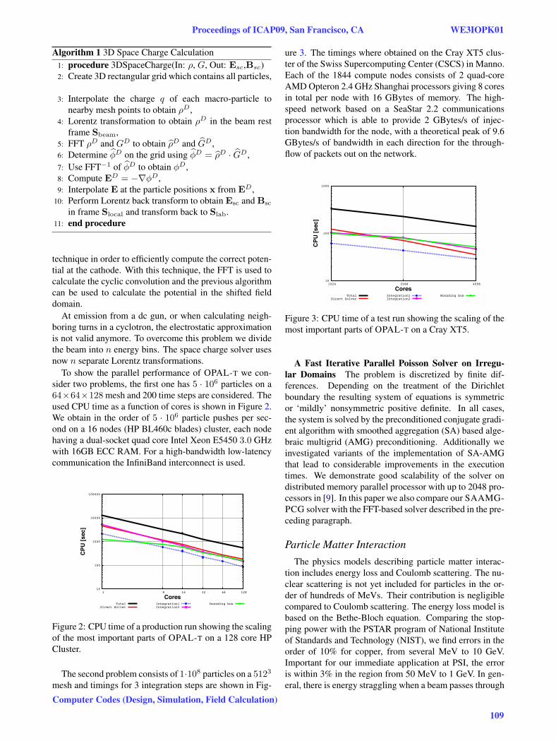
To show the parallel performance of OPAL-T we con-sider two problems, the first one has 5 · 106 particles on a64×64×128 mesh and 200 time steps are considered. Theused CPU time as a function of cores is shown in Figure 2.We obtain in the order of 5 · 106 particle pushes per sec-ond on a 16 nodes (HP BL460c blades) cluster, each nodehaving a dual-socket quad core Intel Xeon E5450 3.0 GHzwith 16GB ECC RAM. For a high-bandwidth low-latencycommunication the InfiniBand interconnect is used.

10

100

1000

10000

100000

128 64 32 16 8 1

CPU

[sec

]

CoresTotal

Direct SolverIntegration1Integration2

Bounding box

Figure 2: CPU time of a production run showing the scalingof the most important parts of OPAL-T on a 128 core HPCluster.

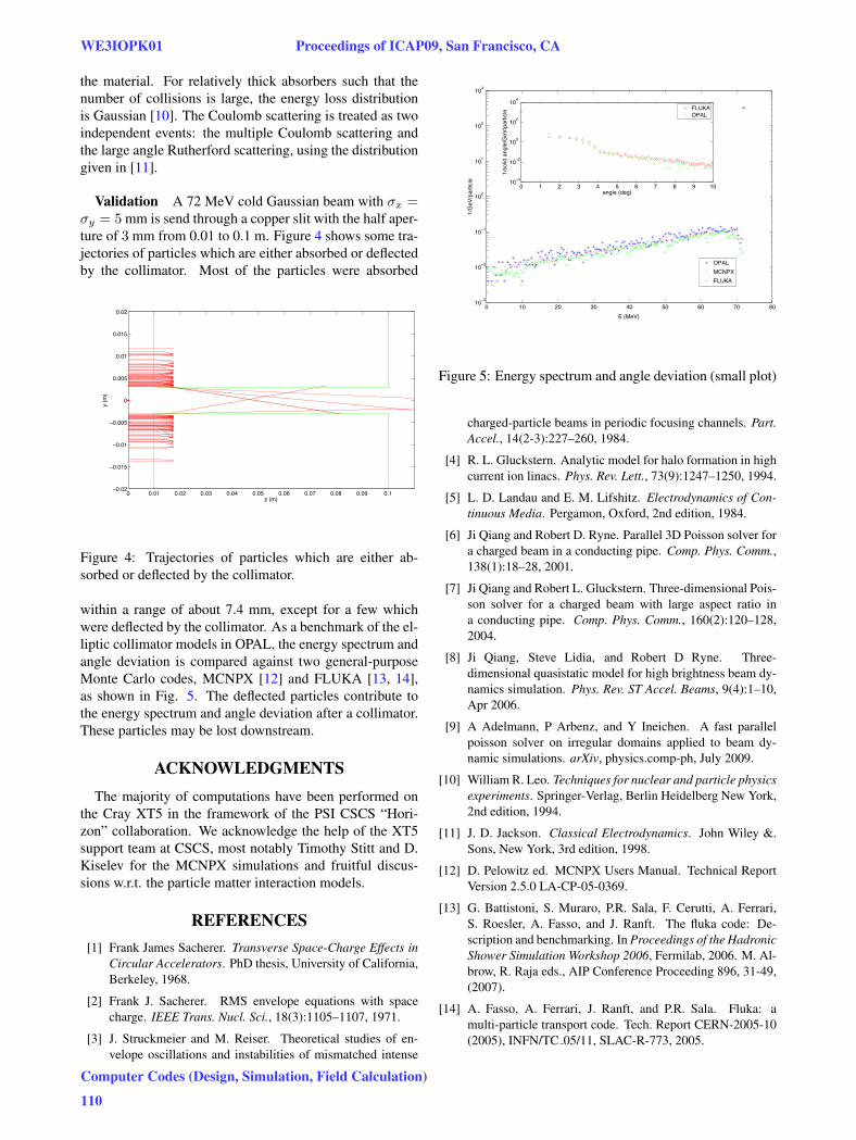
The second problem consists of 1·108 particles on a 5123

mesh and timings for 3 integration steps are shown in Fig-

ure 3. The timings where obtained on the Cray XT5 clus-ter of the Swiss Supercomputing Center (CSCS) in Manno.Each of the 1844 compute nodes consists of 2 quad-coreAMD Opteron 2.4 GHz Shanghai processors giving 8 coresin total per node with 16 GBytes of memory. The high-speed network based on a SeaStar 2.2 communicationsprocessor which is able to provide 2 GBytes/s of injec-tion bandwidth for the node, with a theoretical peak of 9.6GBytes/s of bandwidth in each direction for the through-flow of packets out on the network.

10

100

1000

4096 2048 1024

CPU

[sec

]

CoresTotal

Direct SolverIntegration1Integration2

Bounding box

Figure 3: CPU time of a test run showing the scaling of themost important parts of OPAL-T on a Cray XT5.

A Fast Iterative Parallel Poisson Solver on Irregu-lar Domains The problem is discretized by finite dif-ferences. Depending on the treatment of the Dirichletboundary the resulting system of equations is symmetricor ‘mildly’ nonsymmetric positive definite. In all cases,the system is solved by the preconditioned conjugate gradi-ent algorithm with smoothed aggregation (SA) based alge-braic multigrid (AMG) preconditioning. Additionally weinvestigated variants of the implementation of SA-AMGthat lead to considerable improvements in the executiontimes. We demonstrate good scalability of the solver ondistributed memory parallel processor with up to 2048 pro-cessors in [9]. In this paper we also compare our SAAMG-PCG solver with the FFT-based solver described in the pre-ceding paragraph.

Particle Matter InteractionThe physics models describing particle matter interac-

tion includes energy loss and Coulomb scattering. The nu-clear scattering is not yet included for particles in the or-der of hundreds of MeVs. Their contribution is negligiblecompared to Coulomb scattering. The energy loss model isbased on the Bethe-Bloch equation. Comparing the stop-ping power with the PSTAR program of National Instituteof Standards and Technology (NIST), we find errors in theorder of 10% for copper, from several MeV to 10 GeV.Important for our immediate application at PSI, the erroris within 3% in the region from 50 MeV to 1 GeV. In gen-eral, there is energy straggling when a beam passes through

Proceedings of ICAP09, San Francisco, CA WE3IOPK01

Computer Codes (Design, Simulation, Field Calculation)

109

the material. For relatively thick absorbers such that thenumber of collisions is large, the energy loss distributionis Gaussian [10]. The Coulomb scattering is treated as twoindependent events: the multiple Coulomb scattering andthe large angle Rutherford scattering, using the distributiongiven in [11].

Validation A 72 MeV cold Gaussian beam with σx =σy = 5 mm is send through a copper slit with the half aper-ture of 3 mm from 0.01 to 0.1 m. Figure 4 shows some tra-jectories of particles which are either absorbed or deflectedby the collimator. Most of the particles were absorbed

0 0.01 0.02 0.03 0.04 0.05 0.06 0.07 0.08 0.09 0.1−0.02

−0.015

−0.01

−0.005

0

0.005

0.01

0.015

0.02

z (m)

y (m

)

Figure 4: Trajectories of particles which are either ab-sorbed or deflected by the collimator.

within a range of about 7.4 mm, except for a few whichwere deflected by the collimator. As a benchmark of the el-liptic collimator models in OPAL, the energy spectrum andangle deviation is compared against two general-purposeMonte Carlo codes, MCNPX [12] and FLUKA [13, 14],as shown in Fig. 5. The deflected particles contribute tothe energy spectrum and angle deviation after a collimator.These particles may be lost downstream.

ACKNOWLEDGMENTSThe majority of computations have been performed on

the Cray XT5 in the framework of the PSI CSCS “Hori-zon” collaboration. We acknowledge the help of the XT5support team at CSCS, most notably Timothy Stitt and D.Kiselev for the MCNPX simulations and fruitful discus-sions w.r.t. the particle matter interaction models.

REFERENCES[1] Frank James Sacherer. Transverse Space-Charge Effects in

Circular Accelerators. PhD thesis, University of California,Berkeley, 1968.

[2] Frank J. Sacherer. RMS envelope equations with spacecharge. IEEE Trans. Nucl. Sci., 18(3):1105–1107, 1971.

[3] J. Struckmeier and M. Reiser. Theoretical studies of en-velope oscillations and instabilities of mismatched intense

0 10 20 30 40 50 60 70 8010−3

10−2

10−1

100

101

102

103

E (MeV)

1/G

eV/p

artic

le

OPALMCNPXFLUKA

0 1 2 3 4 5 6 7 8 9 1010−4

10−2

100

102

104

angle (deg)

1/so

lid a

ngle

/GeV

/par

ticle

FLUKAOPAL

Figure 5: Energy spectrum and angle deviation (small plot)

charged-particle beams in periodic focusing channels. Part.Accel., 14(2-3):227–260, 1984.

[4] R. L. Gluckstern. Analytic model for halo formation in highcurrent ion linacs. Phys. Rev. Lett., 73(9):1247–1250, 1994.

[5] L. D. Landau and E. M. Lifshitz. Electrodynamics of Con-tinuous Media. Pergamon, Oxford, 2nd edition, 1984.

[6] Ji Qiang and Robert D. Ryne. Parallel 3D Poisson solver fora charged beam in a conducting pipe. Comp. Phys. Comm.,138(1):18–28, 2001.

[7] Ji Qiang and Robert L. Gluckstern. Three-dimensional Pois-son solver for a charged beam with large aspect ratio ina conducting pipe. Comp. Phys. Comm., 160(2):120–128,2004.

[8] Ji Qiang, Steve Lidia, and Robert D Ryne. Three-dimensional quasistatic model for high brightness beam dy-namics simulation. Phys. Rev. ST Accel. Beams, 9(4):1–10,Apr 2006.

[9] A Adelmann, P Arbenz, and Y Ineichen. A fast parallelpoisson solver on irregular domains applied to beam dy-namic simulations. arXiv, physics.comp-ph, July 2009.

[10] William R. Leo. Techniques for nuclear and particle physicsexperiments. Springer-Verlag, Berlin Heidelberg New York,2nd edition, 1994.

[11] J. D. Jackson. Classical Electrodynamics. John Wiley &.Sons, New York, 3rd edition, 1998.

[12] D. Pelowitz ed. MCNPX Users Manual. Technical ReportVersion 2.5.0 LA-CP-05-0369.

[13] G. Battistoni, S. Muraro, P.R. Sala, F. Cerutti, A. Ferrari,S. Roesler, A. Fasso, and J. Ranft. The fluka code: De-scription and benchmarking. In Proceedings of the HadronicShower Simulation Workshop 2006, Fermilab, 2006. M. Al-brow, R. Raja eds., AIP Conference Proceeding 896, 31-49,(2007).

[14] A. Fasso, A. Ferrari, J. Ranft, and P.R. Sala. Fluka: amulti-particle transport code. Tech. Report CERN-2005-10(2005), INFN/TC 05/11, SLAC-R-773, 2005.

WE3IOPK01 Proceedings of ICAP09, San Francisco, CA

Computer Codes (Design, Simulation, Field Calculation)

110