The North American NanoHertz Observatory of

Gravitational WavesAndrea N. Lommen

Chair, NANOGrav

Associate Professor of Physics and Astronomy

Head of Astronomy Program

Director of Grundy Observatory

Franklin and Marshall College

Lancaster, PA

Image Courtesy of Michael Kramer

• Anne Archibald, McGill University• Zaven Arzoumanian, Goddard Space Flight Center• Don Backer, University of California, Berkeley• Adam Brazier, Cornell University• Jason Boyles, West Virginia University• Brian Burt, Franklin and Marshall College• Jim Cordes, Cornell University• Paul Demorest, National Radio Astronomy Observatory• Justin Ellis, West Virginia University• Rob Ferdman, CNRS, France• L. Samuel Finn, Center of Gravitational Physics at Penn State University• Paulo Freire, National Astronomy and Ionospheric Center• Alex Garcia, University of Texas, Brownsville• Marjorie Gonzalez, University of British Columbia• Rick Jenet, University of Texas, Brownsville, CGWA• Victoria Kaspi, McGill University• Joseph Lazio, Naval Research Laboratories• Andrea Lommen, Franklin and Marshall College• Duncan Lorimer, West Virginia University• Ryan Lynch, University of Virginia• Maura McLaughlin, West Virginia University• Jonathan Nelson, Oberlin College• David Nice, Bryn Mawr College• Nipuni Palliyaguru, West Virginia University• Delphine Perrodin, Franklin and Marshall College• Scott Ransom, National Radio Astronomy Observatory• Ryan Shannon, Cornell University• Xavi Siemens, University of Wisconsin• Ingrid Stairs, University of British Columbia• Dan Stinebring, Oberlin College• Kevin Stovall, University of Texas, Brownsville

Talk represents work with:• NANOGrav• European Pulsar Timing Array• Parkes Pulsar Timing Array

Thrilled with the work of:• A. Sesana, A. Vecchio, M. Volunteri, C. N. Colacino• Melissa Anholm, Xavier Siemens, Larry Price, U.

Milwaukee• Joe Romano, Graham Woan• Chris Messenger, AEI

• r3wkee• Rutger van Haasteren, Yuri Levin, U. Leiden

The International Pulsar Timing Array

What is a

pulsar?

Stability of the clocks

Dominant source of gravitational waves: Binary black hole

Image courtesy of NASA

Pulsar2Pulsar1

Earth

Photo Courtesy of Virgo

Adapted from NASA figure

Hannah Williams, Penn State

Detectability of a Waveform

€

gμυ = ημυ + hμυ

dt

dλ

⎛

⎝ ⎜

⎞

⎠ ⎟2

= δ jk

dx j

dλ

dx k

dλ+

dx j

dλ

dx k

dλh jk t,

r x ( )

dt =∫ dλ −1− kmnm

1+ kmnm∫ dλn j∫ n kh jk t λ( ),r x λ( )( )

Residual = e jknjn k h0

21− kmnm( ) f t0( ) − f t0 − L 1+ kmnm

( )( )[ ]

where h jk t,r x ( ) = h0 ′ f t − ˆ k ⋅

r x ( )e and L is the distance to the pulsar.

The shape of the GW response

Thanks Bill Coles

A sense of what’s detectable

€

h =M

53

P2

3dτ = hP

τ =M

53P

13

d

τ = 50ns

M

2 ×109 MΘ

⎛

⎝ ⎜

⎞

⎠ ⎟

53 P

1year

⎛

⎝ ⎜

⎞

⎠ ⎟

13

d

100Mpc

⎛

⎝ ⎜

⎞

⎠ ⎟

Constraining the Properties of Supermassive Black Hole Systems Using Pulsar Timing: Application to 3C 66b, Jenet, Lommen, Larson and Wen (2004) ApJ 606:799-803.

Data from Kaspi, Taylor, Ryba 1994

15

Orbital Motion in the Radio Galaxy 3C 66B: Evidence for a Supermassive Black Hole Binary Sudou, Iguchi, Murata, Taniguchi (2003) Science 300: 1263-1265.

Re

sid

ual

(ms)

-10

10

0

Re

sid

ual

(ms)

-10

10

0

Simulated residuals due to 3c66b

Figure by Paul Demorest (see arXiv:0902.2968)

MBH-M

BH (indiv)

Gal NS/BH

BH-BH (indiv)

PSRs

Sesana, Vecchio and Volunteri 2009

Maximum Entropy

€

d = n + Rh ⇒ n = d − Rh

p(d | h,k,R,N) =exp −

1

2xT N −1x

⎡ ⎣ ⎢

⎤ ⎦ ⎥

(2π )dim x det N

where

x = d − Rh

entropy :

H( p) = dx n p ln(p)∫

A 5 x 109 solar-mass black hole binary coalescing 100 Mpc away. 30 IPTA pulsars, improved by 10, sampled once a day.

Thank you to Manuela Campanelli, Carlos O. Lousto, Hiroyuki Nakano, and Yosef Zlochowerfor waveforms. Phys.Rev.D79:084010 (2009). http://ccrg.rit.edu/downloads/waveforms

Maximum Entropy based on Summerscales, Burrows, Finn and Ott 2008

Probability density

Log of probability density

2 109 solar mass black holes flying by each other with a separation of 40 Schwarzschild Radii. Distance: 100 Mpc30 IPTA pulsars

Probability density as a function of sky position

Log(probability density) as a function of sky position

The Advantage of New Wide-

band Backend

System at Green Bank

“GUPPI”

Summary

• Pulsars make a galactic scale gravitational wave observatory which is poised to detect gravitational waves in about 10 years.

• Individual and collections of super massive black hole binaries with year-long periods (10s of nHz) are our most considered source.

• In the burst work are pushing the sensitivity of the PTAs to higher GW frequencies (10-5 Hz).

• We can recover the waveform buried in noise.• We recover the direction.• Stay tuned for volume of space covered with current

and future sensitivities.• We expect to be surprised.

Typical Pulsar Model

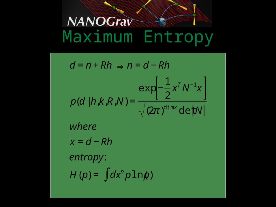
• Measure the polarisation properties of gravitational wave

• Test theories of gravity…!

Lee et al. (2008)

Sensitivity to a 0.75 ms 2-week burst, daily observing, 20 PPTA pulsars

Sensitivity to a 0.75 s 2-week burst, daily observing, 20 PPTA pulsars

Sensitivity to a 0.75 s 2-week burst, daily observing, 20 PPTA pulsars

Sensitivity to a 0.75 s 2-week burst, daily observing, 20 PPTA pulsars + 3 more

So what can we detect?• 20 pulsars, 1 microsecond RMS, daily obs, we

would detect a 0.70 microsecond maximum response about 93% of the time. For a 2-week burst we calculate the corresponding characteristic strain:

Max response (us)

Characteristic strain (h)

Percent detected

0.7 3.3e-13 93

0.5 2.3e-13 40

0.3 1.4e-13 2

Scaling that last slide

• Statistic scales as number of pulsars so e.g. measurable strains halve if number of pulsars doubles

• Response scales as burst length, so measurable strains halve if burst length doubles

• If 20 pulsars have 100 ns RMS, divide left two columns by 10

€

fmin ≈1

dataspan

hc ( fmin ) ≈rms

dataspan

Ωgw ( f ) =2

3

π 2

H02

f 2hc ( f )2

Ωgw ( f )∝rms2

dataspan4

Rms and dataspan are the currency of the field

From Jenet, Hobbs, van Straten, Manchester, Bailes, Verbiest, Edwards, Hotan, Sarkissian & Ord (2006)

Detectability of a Waveform (continued)

So what matters is the integral of the waveform:

€

R = h τ( )0

t

∫ dτ

Sinusoidal source :

R = h0 cos ωτ( )0

t

∫ dτ =h0

ωsin ωt( ) = h0

P

2πsin ωt( )

or a Gaussian source :

R = h0e− τ −tc( ) /σ( )

2

0

t

∫ dτ = h0σ π

Table from NANOGrav white paper (Demorest, Lazio & Lommen, 2009)

€

hc,min =σ

T 3 / 2 N pulsars

General Relativity Gives…