The New Issues Puzzle:

Testing the Investment-Based Explanation

Evgeny Lyandres∗

Jones Graduate School of Management

Rice University

Le Sun†

William E. Simon Graduate School of Business Administration

University of Rochester and GSAM

Lu Zhang‡

Stephen M. Ross School of Business

University of Michigan and NBER

November 2006§

Abstract

An investment factor, long in low investment stocks and short in high investment stocks, helpsexplain the new issues puzzle. Adding this factor into standard factor regressions reduces sub-stantially the magnitude of the underperformance following equity and debt offerings and thecomposite issuance effect. The reason is that issuers invest more than nonissuers, and the low-minus-high investment factor earns a significant average return of 0.57% per month. Our evi-dence lends support to the real options theory, in which investment extinguishes risky expansionoptions, and the q-theory of investment, in which firms with low costs of capital invest more.

∗Jones Graduate School of Management, Rice University, Room 240–MS 531, 6100 Main Street, Houston, TX77005; tel: (713) 348-4708, fax: (713) 348-6296, email: lyandres@rice.edu.

†Simon School of Business, University of Rochester, 500 Wilson Boulevard, Rochester, NY 14627; tel: (585) 275-4318, email: le.sun@simon.rochester.edu, and Goldman Sachs Asset Management, 1 New York Plaza, Floor 40, NewYork, NY 10004; tel: (917) 343-2407, fax: (212) 346-3738, email: le.sun@gs.com.

‡Finance Department, Stephen M. Ross School of Business, University of Michigan, 701 Tappan, ER 7605, AnnArbor MI 48109-1234 and NBER; tel: (734) 615-4854, fax: (734) 936-0282, e-mail: zhanglu@bus.umich.edu.

§We acknowledge helpful comments from Aydogan Alti, Yaakov Amihud, Michael Barclay, Michael Bradley,Michael Brandt, Alon Brav, Bala Dharan, Chris Downing, Evan Dudley, Espen Eckbo, Jeff Fleming, Luis Garcia-Feijoo, Fangjian Fu, Louis Gagnon, Lorenzo Garlappi, Rick Green, John Griffin, Gustavo Grullon, Jay Hartzell,Burton Hollifield, Gautam Kaul, Ambrus Kecskes, Han Kim, Erik Lie, Laura Liu, John Long, Øyvind Norli, JayRitter, David Robinson, Paul Schultz, Richard Sloan, Matt Spiegel, Laura Starks, Paul Tetlock, Sheridan Titman,S. Viswanathan, Jerry Warner, James Weston, Jeff Wurgler, Wei Yang, seminar participants at Duke University,Queens University, Rice University, Texas A&M University, University of Michigan, University of Rochester,University of Texas at Austin, the 2005 UBC Summer Finance Conference, the 2005 European Finance AssociationAnnual Meetings, the 2005 Financial Management Association Annual Meetings, the 2005 Finance and Accountingin Tel-Aviv Conference, and the 2006 CRSP Forum. This paper supercedes our working paper previously entitled“Investment-based underperformance following seasoned equity offerings.” All remaining errors are our own.

1

1 Introduction

Equity and debt issuers underperform matching nonissuers with similar characteristics during the

three to five post-issue years (e.g., Ritter 1991; Loughran and Ritter 1995; and Spiess and Affleck-

Graves 1995, 1999). We explore empirically the investment-based hypothesis of this underper-

formance. The q-theory of investment and real options theory imply a negative relation between

investment and expected returns. If the proceeds from equity and debt issues are used to finance in-

vestment, then issuers should invest more and earn lower average returns than matching nonissuers.

Our central finding is that a new investment factor, long in low investment stocks and short in

high investment stocks, explains a substantial part of the new issues puzzle. Specifically:

• We construct the investment factor by buying stocks with the bottom 30% investment-to-

asset ratios and selling stocks with the top 30% investment-to-asset ratios, while using a

triple sort to control for size and book-to-market. From January 1970 to December 2005, the

investment factor earns an average return of 0.57% per month (t-statistic = 7.13).

• Most importantly, adding the investment factor into standard factor regressions reduces the

magnitude of the underperformance for new equity issues portfolios. The equally-weighted

portfolio of firms that have conducted seasoned equity offerings (SEOs) in the prior 36 months

earns an alpha of −0.41% per month (t-statistic = −2.43). Adding the investment factor

makes the CAPM alpha insignificant and reduces its magnitude by 82% to −0.07% per month.

The equally-weighted portfolio of firms that have conducted initial public offerings (IPOs) in

the prior 36 months earn an alpha of −0.71% per month (t-statistic = −2.60). Adding the

investment factor makes the CAPM alpha insignificant and reduces its magnitude by 59% to

−0.29%. The results from the Fama-French (1993) model are quantitatively similar.

• The investment factor also helps explain the underperformance following debt offerings. The

equally-weighted portfolio of firms that have conducted convertible debt offerings in the prior

36 months earn an alpha of −0.63% per month (t-statistic = −4.20). Adding the invest-

ment factor makes reduces the CAPM alpha by 46% in magnitude to −0.34%, albeit still

significant (t-statistic = −2.04). The underperformance following straight debt offerings is

largely insignificant in our sample. The only exception is the equally-weighted alpha from

the Fama-French (1993) model, −0.26% per month (t-statistic = −2.35). Controlling for the

investment factor makes the alpha weakly positive, 0.029% per month (t-statistic = 0.27).

• The results from using buy-and-hold abnormal returns (BHARs) are largely consistent with

factor regressions. The BHARs of the SEO portfolio from matching on size and book-to-

market over the first two and three post-issue years are −21.9% and −34.6%, respectively.

Matching further on investment-to-asset ratios reduces the BHARs to −16.1% and −25.2%,

respectively, about 26% drop in magnitude. The BHARs of the IPO portfolio from matching

on size and book-to-market are significantly negative after about six post-issue months, and

the BHARs of the convertible debt portfolio are significantly negative after about 18 post-issue

months. Matching on investment-to-asset makes this underperformance largely insignificant.

• The investment factor also explains part of Daniel and Titman’s (2006) finding. A zero-

cost portfolio that buys stocks in the bottom 30% and sells stocks in the top 30% of their

composite equity issuance measure earns an equally-weighted alpha of −0.56% per month

(t-statistic = −4.38) from the CAPM. Adding the investment factor reduces the alpha to

−0.40% (t-statistic = −3.18), a drop in magnitude of 28%. The value-weighted alpha from

the Fama-French (1993) model is −0.36% per month (t-statistic = −3.57), and it drops by

57% in magnitude to −0.16% (t-statistic = −1.49) when we include the investment factor.

Our evidence lends support to the investment-based explanation of the new issues puzzle (e.g.,

Zhang 2005; Carlson, Fisher, and Giammarino 2006). In their real options model, Carlson et al.

argue that firms have expansion options and assets in place prior to equity issuance. This compo-

sition is levered and risky. If real investment is financed by equity, then risk and expected returns

must decrease because investment extinguishes the risky expansion options.

2

Inspired by the negative relation between real investment and expected returns first derived by

Cochrane (1991), Zhang (2005) argues that investment is likely to be the main driving force of the

new issues puzzle. Intuitively, real investment increases with the net present values (NPVs) of new

projects (e.g., Brealey, Myers, and Allen 2006, chapter 6). The NPVs of new projects are inversely

related to their costs of capital or expected returns, controlling for their expected cash flows. If

the costs of capital are high, then the NPVs are low, giving rise to low investment. If the costs

of capital are low, then the NPVs are high, giving rise to high investment. The average costs of

equity for firms that take many new projects are reduced by the low costs of capital for the new

projects. Further, firms’ balance-sheet constraint implies that the sources of funds must equal the

uses of funds. Therefore, firms raising capital are likely to invest more and earn lower expected

returns, and firms distributing capital are likely to invest less and earn higher expected returns.

Consistent with this theoretical prediction, we document that issuers invest more than matching

nonissuers. The investment-to-asset spread between issuers and nonissuers is the highest in the IPO

sample, followed by the SEO and convertible debt sample, and is the lowest in the straight debt

sample. The relative magnitudes of the investment-to-asset spreads are consistent with the relative

magnitudes of the underperformance across the four samples. We also find that high composite

issuance firms invest more than low composite issuance firms.

Our paper brings the insights from the literature on investment-based asset pricing to the liter-

ature on the new issues puzzle. Our use of investment-to-asset as a key matching characteristic is

motivated by the partial equilibrium models of Cochrane (1991, 1996) and Berk, Green, and Naik

(1999). Our use of the investment factor as a common factor of stock returns is motivated by the

general equilibrium models of Gala (2005) and Pastor and Veronesi (2005a, b).

Several papers document the negative relation between investment and average returns. Cochrane

(1991) is among the first to show this relation in the time series. Titman, Wei, and Xie (2004)

and Cooper, Gulen, and Schill (2006) find a similar relation in the cross section but interpret the

evidence as investors underreacting to overinvestment. Xing (2005) shows that real investment

3

helps explain the value effect. Anderson and Garcia-Feijoo (2006) find that investment growth

classifies firms into size and book-to-market portfolios. Anderson and Garcia-Feijoo also anticipate

our analysis: “Many studies examine long-run returns to firms subsequent to new security offerings

and report negative abnormal returns. Benchmarking long-run returns to changes in investment

spending that may coincide with financing events might attenuate abnormal returns (p. 191).”

Brav and Gompers (1997) and Brav, Geczy, and Gompers (2000) document that equity issuers

are concentrated among small-growth firms, and suggest that their underperformance reflects the

Fama-French (1993) size and book-to-market factors. Our evidence supports this argument because

both equity issuers and small-growth firms invest more than other types of firms. We suggest that

real investment is likely to be the common link and the more fundamental driving force of their

underperformance. Eckbo, Masulis, and Norli (2000) show that a six-factor model can explain the

new issues puzzle, but we show that controlling for the investment factor is often sufficient.

The rest of the paper is organized as follows. Section 2 develops the testable hypothesis. Section

3 describes our data. Section 4 reports our empirical results, and Section 5 concludes.

2 Hypothesis Development

The investment-based explanation of the new issues puzzle argues that the post-issue underperfor-

mance arises from the negative relation between real investment and expected returns. First, the

relation between real investment and expected returns is negative. Second, if firms issue new equity

and debt to finance real investment, then issuers should earn lower expected returns than nonissuers.

2.1 Theoretical Motivation

Figure 1 illustrates the negative relation between real investment and expected returns, a central

prediction in recent theoretical literature on investment-based asset pricing. Cochrane (1991, 1996)

derives the negative investment-return relation from the q theory of investment. In his models,

firms invest more when their marginal q—the net present value of future cash flows generated from

4

one additional unit of capital—is high. Controlling for expected cash flows, a high marginal q is

associated with a low cost of capital. In the real options model of Berk, Green, and Naik (1999),

firms invest more when they have access to many low risk projects. Investing in these projects

lowers firm level risk and expected returns. In Carlson, Fisher, and Giammarino (2004), expansion

options are riskier than assets in place. Real investment transforms riskier expansion options into

less risky assets in place, thereby reducing risk and expected returns.1

Figure 1 : The Investment-Based Explanation of the New Issues Puzzle

-Investment-to-asset

6Expected return

0

Issuers: SEO firms

IPO firms

Convertible debt issuers

Straight debt issuers

High composite issuance firms

High investment-to-asset firms

��

��

�

Matching nonissuers

Low composite issuance firms

Low investment-to-asset firms

��

���

The partial equilibrium models discussed above motivate real investment as a characteristic re-

lated to risk. Berk, Green, and Naik (1999), for example, show that high investment firms earn low

average returns because their loadings on the exogenous pricing kernel in their model are low. In

contrast, general equilibrium models help motivate a zero-cost portfolio sorted on real investment

as a systematic, common factor in the cross section of returns.

1The basic mechanisms in the real options and the q-theory models are similar because the two approaches areequivalent (e.g., Abel, Dixit, Eberly, and Pindyck 1996).

5

Gala (2005) constructs a general equilibrium production economy with heterogeneous firms. In

his model, a firm’s ability to provide consumption insurance depends on its ability to mitigate ag-

gregate business cycle shocks through capital investment. In bad times, low investment, value firms

want to disinvest and sell off their capital stocks. But they are prevented from doing so because of

binding irreversibility constraints. These firms thus earn high expected returns because their returns

covary more with economic downturns. In contrast, in the face of negative shocks, high investment,

growth firms can easily lower their positive investment without facing the irreversibility constraints.

These firms thus earn low expected returns as they provide consumption insurance to investors.

Pastor and Veronesi (2005a) develop a general equilibrium model of optimal timing of initial

public offerings, in which IPO waves are partially caused by declines in expected market returns. In

their model, entrepreneurs choose the optimal timing of taking their private firms public, and then

immediately investing part of the equity proceeds. Entrepreneurs prefer to postpone their IPOs

until favorable market conditions such as low expected market return and high expected aggregate

profitability. As a result, real investment of IPO firms can serve as a state variable: high investment

suggests low expected market returns, high aggregate profitability, or both.

Pastor and Veronesi (2005b) develop a general equilibrium model in which returns of firms

investing in new technologies can define new systematic factors. Their model has two sectors: the

“new economy” and the “old economy.” The old economy implements existing technologies on a

large scale and its output determines a representative agent’s terminal wealth. The new economy

implements the new technology on a small scale that does not affect the terminal wealth. The

agent optimally chooses to experiment with the new technology on a small scale to learn about its

unobservable productivity. If the productivity turns out to be sufficiently high, the new technology

is adopted on a large scale. The nature of the risk associated with new technologies changes over

time. The risk is initially idiosyncratic because of the small scale of production. Once adopted on a

large scale, the risk becomes systematic because the new economy now affects the terminal wealth.

6

Figure 1 also shows that issuers are located at the right end of the curve, where expected re-

turns are low, and nonissuers are located at the left end of the curve, where expected returns are

high. Intuitively, the balance-sheet constraint requires that the uses of funds must equal the sources

of funds, implying that issuers are likely to invest more than nonissuers. Based on this insight,

Zhang (2005) and Carlson, Fisher, and Giammarino (2006) argue that SEO firms must earn lower

expected returns than matching nonissuers. The same intuition also applies to the underperfor-

mance following IPOs (e.g., Ritter 1991) and convertible and straight debt offerings (e.g., Spiess

and Affleck-Graves 1999), as well as the composite issuance effect (e.g., Daniel and Titman 2006).

The investment-based explanation of the new issues puzzle, and more generally, the negative

investment-return relation are conditional on a given level of profitability. High investment can

be caused not only by low costs of capital, but also by high expected cash flows (profitability).

More profitable firms earn higher average returns than less profitable firms (e.g., Piotroski 2000;

Fama and French 2006). Our results show that the difference in investment between issuers and

nonissuers, rather than the difference in profitability, drives the new issues puzzle.

2.2 Empirical Design

Our choice of empirical methods echoes the theme of the theoretical motivation by complementing

the use of a zero-cost low-minus-high investment factor as a common factor of stock returns and

the use of investment as a matching characteristic.

Motivated by the partial equilibrium models (e.g., Cochrane 1991; Berk, Green, and Naik 1999),

we examine the performance of security issuers relative to matching firms with similar characteris-

tics including prior investment-to-asset ratios. The theoretical prior is that matching on investment

should reduce the magnitude of buy-and-hold abnormal returns documented in previous studies (in

which investment is not one of the control characteristics). Motivated by the general equilibrium

models (e.g., Gala 2005; Pastor and Veronesi 2005a, b), we augment standard factor regressions

with the investment factor constructed by sorting firms on their investment-to-asset ratios. The

7

theoretical prior is that doing so should reduce the magnitude of the post-issue underperformance.

Following Fama and French (1993, 1996), we interpret the investment factor as a common fac-

tor. While Fama and French go further and interpret their similarly constructed SMB and HML

factors as risk factors motivated from ICAPM or APT, we do not take a stance on the risk inter-

pretation of our investment factor. Arguments supporting the risk interpretation are clear. None

of the theoretical papers that we use to motivate the investment factor assumes any form of over-

and under-reaction. And unlike size and book-to-market, investment-to-asset does not involve the

market value of equity, and is less likely to be affected by mispricing, at least directly.

However, general equilibrium models with behavioral biases (e.g., Barberis, Huang, and Santos

2001) can also motivate the investment factor.2 Moreover, investor sentiment can presumably affect

investment policy through shareholder discount rates (e.g., Polk and Sapienza 2006). Perhaps

more importantly, covariance-based and characteristic-based explanations of the average-return

variations are not mutually exclusive, in contrast to the position taken by Daniel and Titman (1997)

and Davis, Fama, and French (2000). Under certain conditions, there exists a one-to-one mapping

between covariances and characteristics, implying that they can both serve as sufficient statistics

for expected returns (e.g., Zhang 2005). Our goal is thus to search for a theoretically motivated

and empirically parsimonious factor specification that can explain anomalies in asset pricing tests.

3 Data

We examine four types of security offerings: IPOs, SEOs, convertible debt issues, and straight debt

issues. All four samples are obtained from Thomson Financial’s SDC database. The samples of

the IPOs, SEOs, and convertible debt offerings are from 1970 to 2005. Due to data availability, the

sample of the straight debt offerings is from 1983 to 2005. We obtain monthly returns from the

Center for Research in Security Prices (CRSP). The monthly returns of Fama and French’s (1993)

2However, Barberis, Huang, and Santos’s (2001, p. 5) rational expectations model does not admit over- andunder-reaction: “While we do modify the investor’s preferences to reflect experimental evidence about the sourcesof utility, the investor remains rational and dynamically consistent throughout.”

8

three factors and the risk-free rate are from Kenneth French’s website. Accounting information is

from the COMPUSTAT Annual Industrial Files.

Our sample selection largely follows previous studies.3 To be included in a sample, a security

offering must be performed by a U.S. firm that has returns on CRSP at some point during the

three post-issuance years. We exclude unit offerings and secondary offerings of SEOs, in which new

shares are not issued. For SEOs, our results are also robust to the exclusion of mixed offerings.4 We

also exclude equity and debt offerings of firms that trade on exchanges other than NYSE, AMEX,

and NASDAQ. Similar to Brav, Geczy, and Gompers (2000) and Eckbo, Masulis, and Norli (2000),

but different from Loughran and Ritter (1995) and Spiess and Affleck-Graves (1995, 1999), we

include utilities in our sample. Following Loughran and Ritter, we define utilities as firms with

SIC codes ranging between 4,910 and 4,949. Excluding utilities does not materially impact our

results, likely because the fraction of utilities in each sample is small: 6% for SEOs, 0.4% for IPOs,

2% for convertible debt issues, and 8% for straight debt issues. Further, many firms issue multiple

tranches of debt on the same date. We deal with this issue by aggregating the amount issued on a

given day but separating straight and convertible debt issues.

Table 1 reports for each of the four samples the number of offerings for each year, the number of

offerings by non-utilities, and the number of offerings with valid data on size, book-to-market, and

investment-to-asset ratio. These characteristics are used to select matching nonissuers. Our samples

include 10,084 SEOs, 7,732 IPOs, 1,215 convertible debt offerings, and 2,969 straight debt offerings.

Because of the long sample period (22 years for straight debt offerings and 36 years for all others),

our samples are among the largest in the literature. For comparison, Eckbo, Masulis, and Norli’s

(2000) sample includes 4,766 SEOs, Loughran and Ritter’s (1995) sample consists of 3,702 SEOs and

4,753 IPOs, and Brav, Geczy, and Gompers’s (2000) sample includes 4,526 SEOs and 4,622 IPOs. In

3These studies include Loughran and Ritter (1995), Spiess and Affleck-Graves (1995), Eckbo, Masulis and Norli(2000), Brav, Geczy and Gompers (2000), Mitchell and Stafford (2000) for SEOs; Loughran and Ritter (1995), Brav,Geczy and Gompers (2000) for IPOs; Spiess and Affleck-Graves (1999) for straight and convertible debt offerings.

4A mixed offering is a combination of a primary offering, in which new shares are issued, and a secondary offering,in which shares change ownership but no new equity is issued.

9

addition, Spiess and Affleck-Graves’s (1995) sample consists of 1,247 SEOs, and Spiess and Affleck-

Graves’s (1999) samples contain 1,557 straight debt offerings and 672 convertible debt offerings.

To study the frequency distribution of issuers across size and book-to-market quintiles, we as-

sign issuers to quintiles using the breakpoints from Kenneth French’s website. For firms that have

issued in the period from July of year t to June of year t+1, we determine the size and book-to-

market quintiles at the fiscal yearend of calendar year t−1. If size or book-to-market is missing at

that time (frequently in the IPO sample), we use the first available size and book-to-market if the

available date is no later than 12 months after the offering (24 months for IPOs).

We measure the market value as the share price at the end of June times shares outstanding.

Book equity is stockholder’s equity (item 216) minus preferred stock plus balance sheet deferred

taxes and investment tax credit (item 35) if available, minus post-retirement benefit asset (item 330)

if available. If stockholder’s equity is missing, we use common equity (item 60) plus preferred stock

par value (item 130). If these variables are missing, we use book assets (item 6) less liabilities (item

181). Preferred stock is preferred stock liquidating value (item 10), or preferred stock redemption

value (item 56), or preferred stock par value (item 130) in that order of availability. To compute

the book-to-market equity, we use December closing price times number of shares outstanding.

Table 2 presents the frequency distribution of issuing firms and the relative amount of capital

raised in the offerings. From the left four panels, small firms are more likely than large firms to

issue equity and convertible debt, but are less likely to issue straight debt. Growth firms are more

likely than value firms to issue equity and convertible debt, and to a lesser extent, straight debt.

From Panel A, small-growth firms perform 19% of SEOs, while big-value firms account for only

0.52% of SEOs. The spread in issuing frequency is even wider for IPOs: 32% of IPOs are conducted

by small-growth firms, in contrast to only 0.11% by big-value firms. The frequency distribution of

the convertible debt offerings sample is similar to that of the SEO sample. 12% of the convertible

debt issues are performed by small-growth firms, in contrast to only 0.58% undertaken by big-value

firms. Prior studies show that small-growth firms have higher investment-to-asset ratios than other

10

firms (e.g., Xing 2005; Anderson and Garcia-Feijoo 2006). Our evidence that small-growth firms

are also the most frequent equity and convertible debt issuers is therefore suggestive of the role of

real investment in explaining the underperformance following the offerings.5

The right four panels of Table 2 report the median new issue-to-asset ratios of issuers by size and

book-to-market quintiles. We measure the new issue-to-asset ratio as the proceeds of a new issue

from SDC divided by the book value of assets at the fiscal yearend preceding an SEO or convertible

or straight debt offering. Because of data limitations, we use the book value of assets at the fiscal

yearend of an IPO. The distribution of the median new issue-to-asset across size and book-to-market

quintiles is similar to the frequency distribution reported in the left panels of the table. Not only

small-growth firms issue securities much more frequently than big-value firms, but they also issue

much more as a percentage of their book assets. From Panel A, the median new seasoned equity-

to-asset ratio of small-growth firms is 0.89. In contrast, the median ratio of big-value firms is only

0.01. Dispersions of similar magnitudes are also evident in the convertible and straight debt samples

(Panels C and D). From Panel B, the IPO sample displays an even wider spread: the median new

equity-to-asset ratio for small-growth firms is 1.75, much higher than that for big-value firms, 0.05.

4 Empirical Results

We study the role of investment in driving the new issues puzzle using factor regressions (Section

4.1) and buy-and-holding abnormal returns (Section 4.2). Section 4.3 examines the investment and

profitability behavior for issuers and matching nonissuers. Inspired by Daniel and Titman (2006),

Section 4.4 studies the link between investment and the returns of composite issuance portfolios.

4.1 Factor Regressions

Evidence on the New Issues Puzzle

We measure the post-issue underperformance as Jensen’s alphas in factor regressions. Lyon, Barber

and Tsai (1999) argue that factor regressions are one of the two methods that yield well-specified

5Brav, Geczy and Gompers (2000) report similar frequency distributions for SEO and IPO samples.

11

test statistics. (The other approach is Buy-and-Hold Abnormal Returns, see Section 4.2.)

We use the CAPM and the Fama and French (1993) three-factor model. The dependent variables

in the factor regressions are the new issues portfolio returns in excess of the one-month Treasury

bill rate. The new issues portfolios, including the SEO, IPO, convertible debt, and straight debt

portfolios, consist of all firms that have issued seasoned equity, gone public, issued convertible debt,

and issued straight debt in the past 36 months, respectively.6 Loughran and Ritter (2000) argue

that the power of the tests can be increased if we weight each firm equally, instead of weighting

each period equally. Following Spiess and Affleck-Graves (1999), we thus estimate factor regressions

using Weighted Least Squares (WLS), where the weight of each month corresponds to the number

of event firms having non-missing returns during that month.7

Table 3 reports strong evidence of underperformance following equity issuance (Panels A and

B). From Panel A, the equally-weighted alpha from the CAPM regression of the SEO portfolio is

−0.41% per month (t-statistic = −2.43), and that from the Fama-French (1993) model is −0.39%

per month (t-statistic = −3.52). The value-weighted alphas are similar in magnitude. From Panel

B, the post-issue underperformance of IPOs from the CAPM is larger in magnitude than that of

SEOs. The equally-weighted and value-weighted CAPM alphas of the IPO portfolio are −0.71%

and −0.82% per month with t-statistics −2.60 and −3.03, respectively. The alphas of the IPO

portfolios from the Fama-French model are close to those of the SEO portfolios.

Table 3 also reports reliable evidence of post-issue underperformance of convertible debt issuers,

but not of straight debt issuers (Panels C and D). Convertible debt issuers show comparable under-

performance to equity issuers. The convertible debt portfolio earns equally-weighted alphas from

the CAPM and the Fama-French (1993) model of −0.63% and −0.54% per month, respectively.

Both have t-statistics above four. The value-weighted alphas are smaller in magnitude, −0.44%

and −0.26%, but still significant (t-statistics −3.38 and −2.00), respectively. In contrast, only the

equally-weighted alpha from the Fama-French model, −0.26%, is significant for the straight debt

6Using firms that have issued in the prior 60 months yields similar results (not reported).7Estimating the regressions using Ordinary Least Squares does not materially change our results (not reported).

12

portfolio (t-statistic = −2.35). All the other alphas are insignificantly different from zero. Our

evidence that convertible debt issuers display higher post-issue underperformance than straight

debt issuers is consistent with Spiess and Affleck-Graves (1999).

The Investment Factor

As a direct test of the investment hypothesis, we augment traditional factor models with a common

factor based on real investment. We construct the investment factor as the zero-cost portfolio from

buying stocks with the lowest 30% investment-to-asset ratios and selling stocks with the highest

30% investment-to-asset ratios, while controlling for size and book-to-market.

We measure investment-to-asset as the annual change in gross property, plant, and equipment

(COMPUSTAT annual item 7) plus the annual change in inventories (item 3) divided by the lagged

book value of assets (item 6). We use property, plant, and equipment to measure real investment

in long-lived assets used in operations over many years such as buildings, machinery, furniture,

computers, and other equipment. We use inventories to measure real investment in short-lived assets

used in a normal operating cycle such as merchandise, raw materials, supplies, and work in process.

We do a triple sort on size, book-to-market, and investment-to-asset a la Fama and French

(1993). We independently sort stocks in each June on size, book-to-market, and investment-to-asset

into three groups, the top 30%, the medium 40%, and the bottom 30%. By taking intersections

of these nine portfolios, we classify stocks into 27 portfolios. The investment factor, denoted INV,

is defined as the average return of the nine low investment-to-asset portfolios minus the average

return of the nine high investment-to-asset portfolios.8

In untabulated results, the investment factor earns an average return of 0.57% per month

(t-statistic = 7.13) from January 1970 to December 2005. This average return is economically

meaningful. For comparison, the average market excess return over the same period is 0.50% per

month (t-statistic = 2.28) and the average HML return is 0.48% per month (t-statistic = 3.24).

8Let pijk denote the value-weighted returns of portfolios consisting of firms in the ith group of size, the jth groupof book-to-market, and the kth group of investment-to-asset, where i, j, k = 1, 2, 3. The investment factor is definedas: INV=(1/9)

P3i=1

P3j=1 pij1−(1/9)

P3i=1

P3j=1 pij3.

13

More importantly, standard factor models cannot capture much of the investment factor’s aver-

age return or its variation. Regressing the investment factor on the market excess return and the

Fama-French (1993) three factors yields alphas of 0.64% and 0.62% per month (t-statistics = 6.98

and 5.67), respectively. The R2 is 12.44% in the CAPM regression and 13.05% in the Fama-French

regression. The evidence suggests that the investment factor captures cross-sectional variations in

returns largely independent of the commonly used factors.

Factor Regressions Augmented with the Investment Factor

Table 4 reports our central finding. Adding the investment factor into standard factor regressions

makes the new issues puzzle often insignificant and reduces its magnitude by 60% on average.

From Panel A of Table 4, the equally-weighted alpha of the SEO portfolio from the CAPM

regression decreases by 82% in magnitude from −0.41% to −0.07% per month, and its t-statistic

drops from −2.43 to −0.40. The equally-weighted alpha from the Fama-French (1993) model de-

creases in magnitude from −0.39% to −0.08% per month, a reduction of 78%, with its t-statistic

dropping from −3.52 to −0.72. The results are similar for the value-weighted returns. The value-

weighted CAPM alpha decreases from −0.44% without the investment factor to −0.14% with the

investment factor, a reduction of 68% in magnitude, with the t-statistic falling from −3.76 to

−1.09. The value-weighted Fama-French alpha drops from −0.35% to −0.05%, a reduction of 85%

in magnitude, and its t-statistic declines from −3.04 to −0.44.

Panel A of Table 4 also shows that the loadings of the SEO portfolios on the investment factor

are all negative and significant. With magnitudes ranging from −0.38 to −0.44, these loadings are

economically important. Given the average return of 0.57% per month for the investment factor,

these loadings account for 0.22–0.25% per month of the SEO underperformance.

The results for the IPOs are similar. From Panel B of Table 4, the equally-weighted CAPM

alpha of the IPO portfolio decreases by 59% from −0.71% to −0.29% per month and its t-statistic

drops from −2.60 to −0.84. The value-weighted alpha decreases from −0.82% to −0.13% per

14

month, a reduction of 84% in magnitude. Its t-statistic falls from −3.03 to −0.36. The results from

the Fama-French (1993) regressions are similar. The equally-weighted alpha decreases in magni-

tude from −0.43% to −0.05%, a reduction of 88%, with a drop in the t-statistic from −2.18 to

−0.21. The value-weighted alpha changes from a marginally significant −0.45% to an insignificant

0.21%. The investment factor loadings of the IPO portfolios are all negative and mostly significant.

With magnitudes ranging from −0.44 to −0.73, these loadings are economically important and they

account for 25–42 basis points per month of the IPO underperformance.

The role of real investment in explaining the post-issue performance of convertible debt offerings

is also sizable. Panel C of Table 4 shows that the equally-weighted CAPM alpha of the convertible

debt portfolio decreases by 46% from −0.63% to −0.34%, albeit remaining significant (t-statistic

= −2.02). The equally-weighted alpha from the Fama-French (1993) model decreases by 31% from

−0.54% to −0.37% (t-statistic = −3.26). The value-weighted results are somewhat stronger. The

CAPM alpha decreases in magnitude by 55% from −0.44% to −0.20% per month, and the Fama-

French alpha drops in magnitude by 72% from −0.26% to −0.07%. After adding the investment

factor, both value-weighted alphas are no longer significant. The loadings of the convertible debt

issuers on the investment factor are all negative and significant. Ranging from −0.25 to −0.41,

these loadings explain 14–24 basis points per month of the post-issue underperformance.

From Panel D of Table 3, the underperformance of straight debt issuers is significant only in the

case of the equally-weighted Fama-French (1993) alpha, −0.26% per month (t-statistic = −2.35).

From Panel D of Table 4, adding the investment factor makes the alpha insignificantly positive.

Event-Time Factor Regressions

To provide more detailed evidence on the role of the investment factor in explaining the new issues

puzzle, we perform event-time factor regressions a la Ball and Kothari (1989). In contrast to having

only one portfolio for a given type of security in calender-time regressions, in event-time regressions

we construct six different new issues portfolios for a given type of security. The first portfolio in

15

event-time regressions consists of firms that have issued in the prior six months, the second portfolio

consists of firms that have issued between seven and 12 months ago, and so on. The last portfolio

consists of firms that have issued between 31 and 36 months ago.

Figure 2 reports the event-time alphas of the new issues portfolios from the Fama-French (1993)

factor regressions, with and without the investment factor (a thick broken line and a thick solid

line respectively; thin broken and solid lines correspond to two-standard-error bounds). Using the

CAPM instead of the Fama-French model yields largely similar results (not reported). The three

broken lines in Panel A show that the underperformance of the equally-weighted SEO portfolio

appears mostly in the second and third post-issue years. The magnitude of the underperformance

from post-event month 13 to 30 is around 0.60% per month and significant with the most severe

underperformance, 0.77%, appearing during months 13–18. Comparing the thick solid line and

the thick broken line in Panel A reveals that the investment factor helps explain the post-issue

alphas. The worst underperformance, during months 13–18, drops by 53% to an insignificant level

of −0.36% per month. In addition, the alphas in post-issue months 19–24 and 25–30 are close to

zero and none of the alphas in the regressions augmented with the investment factor is significant.

Using the value-weighted returns in Panel E yields largely similar results.

The investment factor also plays an important role in explaining the IPO underperformance.

From Panel B of Figure 2, the equally-weighted underperformance of IPO portfolios appears mostly

in months 7–24 post-issue with its magnitude ranging from 0.47% per month during months 19–24

to 0.79% during months 7–12 (the thick broken line). Adding the investment factor eliminates

the significance of this underperformance, and reduces its magnitude by 42% to 0.45% per month

during months 7–12 and by 99% to 0.004% during months 19–24. From Panel F, although the

value-weighted IPO underperformance is largely insignificant, its average magnitude of around

0.50% per month from month 13 to 30 is economically important. Controlling for the investment

factor eliminates this economic importance.

Panels C and G of Figure 2 show that the investment factor plays a more modest role in captur-

16

ing the underperformance following convertible debt offerings. Although it goes in the right direc-

tion, the difference in magnitudes of the underperformance with and without the investment factor

is small. The straight debt portfolio shows significant underperformance during months 13–18 using

equally-weighted returns (Panel D) but not using value-weighted returns (Panel H). From Panel

D, the investment factor largely eliminates the significant equally-weighted underperformance.

4.2 Buy-and-Hold Abnormal Returns

Having documented the importance of the investment factor in explaining the negative alphas of the

new issues portfolios, we now evaluate the importance of investment as a matching characteristic.

We use the buy-and-hold abnormal returns (BHARs) relative to the benchmark returns of reference

portfolios (e.g., Lyon, Barber, and Tsai 1999). Consistent with factor regressions, matching on real

investment helps explain the new issues puzzle.

We compare BHARs obtained by using two reference portfolios.9 We construct the first refer-

ence portfolio by matching each event firm to a portfolio of firms that (i) have not issued a given

type of security in the prior three years, and (ii) belong to the same size and book-to-market quin-

tiles as the event firm. To construct the second reference portfolio, we match each event firm to

a portfolio of firms that (i) have not issued a given type of security in the prior three years, and

(ii) belong to the same size, book-to-market, and investment-to-asset quintiles as the event firm.

The size and book-to-market breakpoints are from Kenneth French’s website. We calculate the

investment-to-asset breakpoints using all firms that have valid investment-to-asset data.

We match firms on size and book-to-market, with and without matching on investment-to-asset.

The reason is that, as argued by Lyon, Barber and Tsai (1999), firms from non-random samples

should be compared to the general population on the basis of characteristics that are the best at

explaining the cross section of returns. Size and book-to-market are two such characteristics.

We follow Lyon, Barber, and Tsai (1999) to construct the reference portfolios and calculate the

9We use BHARs, as opposed to cumulative abnormal returns (CARs) because the latter are biased predictors ofthe long-run abnormal returns (e.g., Barber and Lyon 1997).

17

BHARs in a way that is sensitive to the new listing bias, the rebalancing bias, and the skewness

bias.10 We assign firms to a reference portfolio only once for each event. We do so in the month of

issuance or in the first post-issue month when the size and book-to-market data become available

for an event firm, but no later than 12 post-issue months (24 post-issue months for IPOs). Once

constructed, the composition of a reference portfolio does not change throughout the period of

abnormal return calculation, except for delisted firms. Following Lyon et al., we fill the returns of

delisted firms with the average monthly returns of the remaining firms in the reference portfolios.

To calculate the BHARs, we first calculate the buy-and-hold returns (BHR) for each event firm

for a period ranging from one month to 36 months: BHRiτ =∏τ

t=1 (1 + Riτ ) − 1, where i is the

event-firm index, and τ is the horizon over which BHR is computed. We then compute the buy-

and-hold returns for a reference portfolio as: BHRpiτ =∑npi

j=1

Qτt=1(1+R

pijt )−1

npi, where pi is the index

for the reference portfolio of the event firm i, npiis the number of firms in the reference portfolio,

and Rpi

jt is the return of firm j in the reference portfolio pi during the event-month t. And we

calculate the mean BHARs as: BHARτ =PNτ

k=1(BHRkτ−BHRpkτ )

Nτ, where Nτ is the number of event

firms that have BHRs at the event-month τ .

Because long-horizon abnormal returns are positively skewed (e.g., Barber and Lyon 1997; Lyon,

Barber and Tsai 1999), standard t-statistics are negatively biased. To eliminate this skewness bias,

we follow Lyon et al. and use the skewness-adjusted t-statistics: tτ =√

Nτ (S + 13 γS2 + 1

6Nτγ), where

S = BHARτ

σ(BHRiτ−BHRpiτ ) and σ(BHRiτ −BHRpiτ ) is the standard deviation of abnormal returns for the

sample of Nτ event firms. γ =PNτ

i=1((BHRiτ−BHRpiτ )−BHARτ )3

Nτ σ(BHRiτ−BHRpiτ )3is an estimate of the skewness.

√NτS

is the conventional t-statistic of BHARs.

Figure 3 reports the BHARs of new issues portfolios during the five post-issue years. From

Panel A, the BHARs of seasoned equity issuers over the first two and three post-issue years are

10The new listing bias arises because sample firms are tracked for a long post-event period, while firms thatconstitute the reference portfolio include firms that begin trading subsequent to the event month. The rebalancingbias arises because the compounded returns of a reference portfolio are calculated with periodical rebalancing, butthe returns of sample firms are compounded without rebalancing. The skewness bias occurs because the distributionof long-run abnormal stock returns is positively skewed. The new listings create a positive bias in test statistics butthe rebalancing and skewness create a negative bias. See Lyon, Barber, and Tsai (1999) for details.

18

−21.9% and −34.6%, respectively (the thick solid line). Matching on investment-to-asset reduces

the magnitudes of the BHARs by about 26% to −16.1% and −25.2%, respectively (the thick bro-

ken line). However, the BHARs remain highly significant. Panel B shows a more important role of

real investment in driving the IPO underperformance. Matching on size and book-to-market yields

significantly negative BHARs for the IPO portfolio, for example, −10.6% by year two and −20.8%

by year four. Additional matching on investment-to-asset eliminates this underperformance.

From Panel C of Figure 3, controlling for investment-to-asset helps explain the underperfor-

mance following convertible debt offerings. The BHARs obtained by using size and book-to-market

reference portfolio are −15.8% and −20% after three and five post-issue years, respectively. Con-

trolling for investment-to-asset reduces this underperformance by 41% and 52% to −9.4% and

−9.6%, respectively. Judging from the two thin solid lines, the size and book-to-market post-

issue BHARs of convertible debt issuers become significant after around month 18. Matching on

investment-to-asset largely eliminates this significance (see the two thin broken lines).

Panel D of Figure 3 shows that investment also helps explain the post-issue underperformance

of straight debt issuers. The underperformance from matching on size and book-to-market is

7.3% and 11.4% by months 24 and 36, respectively. Controlling for investment-to-asset reduces

this underperformance by 39% and 46% to 4.4% and 6.2%, respectively. From the two thin solid

lines, the post-issue BHARs of straight debt issuers are significant after month 12. Matching on

investment-to-asset largely eliminates this significance.

Although our empirical procedure is robust to an array of potential biases identified by Lyon,

Barber, and Tsai (1999), the evidence from BHARs is subject to the pseudo-market-timing bias of

Schultz (2003). Schultz argues that event studies are likely to result in negative ex-post abnormal

performance, even though there is no ex-ante underperformance. If early in a sample period, is-

suers underperform, there will be few issues in the future because investors would be less interested

in them. The average performance will be weighted more towards the early issues that underper-

formed. If early issues outperform, there will be more issues in the future. The early positive abnor-

19

mal performance will be weighted less in the average performance. This argument may explain why

our tests are more successful in using the investment factor to reduce the SEO underperformance

in factor regressions than in using the investment-to-asset characteristic to reduce the BHARs.11

4.3 Why Does Real Investment Help Explain the New Issues Puzzle?

To understand the driving forces behind our results, we now examine the investment and profitabil-

ity behavior for issuers and matching nonissuers with similar size and book-to-market.

Real Investment

To preview the results, issuers invest more than matching nonissuers for two to three years after

issuance. The investment-to-asset spread between issuers and matching nonissuers is the highest in

the IPO sample, followed by the SEO and convertible debt samples, and is the lowest in the straight

debt sample. Because of the significantly positive average return of the low-minus-high investment

factor (0.57% per month), the investment-to-asset spread helps explain the new issues puzzle. The

relative magnitude of the investment-to-asset spread is also in line with the relative magnitude of

the underperformance across samples. The underperformance is the highest for IPOs, followed by

SEOs and convertible debt issues, and is the lowest for straight debt issues (see Table 3).

To identify the matching portfolio for each issuer of a given type of security, we sort indepen-

dently all firms that have not issued this type of security in the prior 36 months into size and book-

to-market quintiles in each June. We use the breakpoints from Kenneth French’s website to identify

the matching portfolio for each issuer out of the 25 size and book-to-market portfolios. We then

compare the median investment-to-asset ratios of the matching portfolios with those of the issuers.

Figure 4 reports the median investment-to-asset ratios for issuers and matching nonissuers

during the five post-issue years. Panel A documents a large investment-to-asset spread between

seasoned equity issuers and matching nonissuers. In the first two post-issue years, SEO firms have

a median investment-to-asset ratio of around 0.15, while the matching nonissuers have a median

11Barber and Lyon (1997), Kothari and Warner (1997), Fama (1998), Mitchell and Stafford (2000), and Butler,Grullon, and Weston (2005) also discus the difficulties of computing unbiased inferences using buy-and-hold returns.

20

investment-to-asset ratio of approximately 0.09, about 40% lower. This spread remains stable for

two years after issuance, and converges to zero around month 36.

The IPO sample displays a more dramatic investment-to-asset spread between issuers and nonis-

suers. Panel B of Figure 4 shows that during the first six post-issue months, the investment-to-asset

ratio of IPO firms is around 1.20, about 12 times of the level of matching nonissuers around 0.10.

The investment-to-asset ratio declines rapidly for the IPO firms in the post-event window; it drops

to 0.60 by month 12, to 0.30 by month 24, and largely converges to that of nonissuers by month 36.

Panel C of Figure 4 reports quantitatively similar results for the convertible debt sample as

those for the SEO sample. In the first two post-issue years, convertible debt issuers have a median

investment-to-asset ratio of around 0.17, while the matching nonissuers have a median investment-

to-asset ratio of around 0.11, about 35% lower. The spread converges to zero around month 36.

From Panel D, the investment-to-asset spread between straight debt issuers and matching nonis-

suers is only about 0.01 during the first two post-issue years, and is negative afterwards.12

Supplementing Figure 4, Table 5 reports the frequency distribution of issuers across investment-

to-asset deciles. We sort nonissuing firms in each June on their investment-to-asset ratios to obtain

the decile breakpoints, and then assign each issuer to one of the deciles based on the breakpoints.

Consistent with Figure 4, Table 5 shows that equity and convertible debt issuers are more likely

to be firms with high investment-to-asset ratios. 60.7% of the IPOs are conducted by firms in the

highest investment-to-asset decile, compared to only 5.5% conducted by firms in the lowest decile

(Panel B). Similar but less dramatic patterns appear in the SEO and convertible debt samples.

Specifically, 17.5% and 15.9% of the SEOs and convertible debt offerings are conducted by firms

in the highest investment-to-asset decile, while only 7.8% and 4.9% are conducted by firms in the

lowest decile, respectively (Panels A and C). The distribution of straight debt issuers does not

display a monotonic relation with the investment-to-asset ratio (Panel D).

12We also follow Loughran and Ritter (1997) and use Wilcoxon matched-pairs signed-rank tests to measurestatistical significance of the investment-to-asset spread. The spread is significant across all samples, including thestraight debt sample during the first two post-event years (not reported).

21

Our evidence complements that of Loughran and Ritter (1997), who document that seasoned

equity issuers have higher ratios of capital expenditure plus R&D expense to book assets than non-

issuers for four years after issuance. Their Figure 1 shows that this ratio is about 10% for issuers

and 6.5% for nonissuers in the first two post-issue years. A comparison with our evidence reveals

that this spread is mostly driven by real investment because we do not include R&D expense. (We

also present similar evidence from the IPO, convertible and straight debt samples.)

This difference is conceptually important. Our empirical analysis is partially motivated by the

theoretical work of Zhang (2005) and Carlson, Fisher, and Giammarino (2006), who study the rela-

tion between average returns and real investment (not R&D). Unlike the negative relation between

investment-to-asset and average returns, the relation between R&D-to-asset and average returns is

positive (e.g., Chan, Lakonishok and Sougiannis 2001; Chambers, Jennings, and Thompson 2002;

Eberhart, Maxwell, and Siddique 2004). Chu (2005) argues that the reason is that R&D generates

growth options, while real investment extinguishes them.

Profitability

Figure 5 reports event-time profitability for issuers and nonissuers in the five post-issue years. We

measure profitability as net income before extraordinary items (COMPUSTAT item 18) divided

by the lagged book value of equity. (Our measure of book equity is described in Section 3.) We

find that issuers are more profitable than matching nonissuers, but the profitability spread is much

smaller in magnitude than the investment-to-asset spread.

Panel A of Figure 5 shows that, in the first two post-issue years, the profitability spread be-

tween seasoned equity issuers and matching nonissuers is 0.01, only about 10% of the profitability

of nonissuers. This spread converges to zero around month 32. From Panel B, IPO firms have

a median profitability of 0.24, about three times of nonissuers’ median profitability, 0.08, in the

first six post-issue months. But even this profitability spread is small compared to the spread in

investment-to-asset: IPO firms invest roughly ten times more than nonissuers during the same

22

post-event period (Panel B of Figure 4). The profitability spread between IPO firms and matching

nonissuers converges to zero around month 18. Their investment-to-asset spread, on the other

hand, is still around 0.40 per annum at month 18, and only converges to zero around month 36.

Similar results also apply to the convertible debt sample. In contrast to the sizable investment-

to-asset spread in Panel C of Figure 4, Panel C of Figure 5 shows that the profitability spread is

less than 10% of the nonissuers’ profitability in the first two post-issue years, compared to about

40% investment-to-asset spread in the corresponding period. Comparing Panel D of Figures 4

and 5, both the profitability and investment spreads between straight debt issuers and matching

nonissuers are around 10% of the corresponding nonissuers’ medians.

The evidence on profitability is important. As argued in Section 2, the negative relation between

investment-to-asset and average returns is conditional on profitability. Collectively, Figures 4 and

5 show that the spreads between issuers’ and nonissuers investment levels are much larger than the

spreads in their profitability levels for equity and convertible debt issues, but not for straight debt is-

sues. This evidence thus helps interpret the larger magnitudes of the underperformance following eq-

uity and convertible debt offerings than the underperformance following straight debt offerings, and

the stronger effect of controlling for investment on reducing the magnitude of the underperformance.

4.4 Composite Issuance

Our analysis so far has focused on underperformance following various types of equity and debt

issues. We now integrate the pieces of evidence by examining the role of investment in reducing the

abnormal returns of high-minus-low composite issuance portfolios (e.g., Daniel and Titman 2006).

Our main finding in this subsection is that the investment factor helps explain 28%–57% of the

composite issuance effect, depending on specific test procedure.

Daniel and Titman (2006) define the composite (equity) issuance, denoted ιi(t − τ, t), for firm

i in year t as the growth in the market value of equity not attributable to stock returns:

ιi(t − τ, t) = log

(MEit

MEit−τ

)− ri(t − τ, t) (1)

23

where MEit is the market equity at year t and ri(t− τ, t) is the stock return from year t− τ to year

t. Equity issuance activity such as seasoned equity issues, employee stock option plans, share-based

acquisitions increase ι, while repurchase activity such as share repurchases and dividends reduce ι.

Daniel and Titman (2006) find that a zero-investment portfolio long in stocks with high compos-

ite equity issuance measures and short in stocks with low composite equity issuance measures earns

significantly negative average returns. Daniel and Titman interpret this evidence as investors over-

reacting to intangible information—defined as the component of news about future stock returns

unrelated to past accounting performance—and managers timing their issues and repurchases to ex-

ploit this mispricing. Managers tend to issue shares following the realization of favorable intangible

information and repurchase shares following the realization of unfavorable intangible information.

We explore the investment-based explanation of the composite issuance effect. If firms with

high composite issuance invest more than firms with low composite issuance, the negative relation

between investment and expected returns can at least partially explain Daniel and Titman’s (2006)

evidence. Our test design is simple. After measuring the composite issuance effect using factor re-

gressions, we examine how augmenting the regressions with the investment factor affects the alphas.

We also extend Daniel and Titman’s (2006) analysis and examine the combined effect of debt

issuance on returns by constructing the composite debt issuance measure. For firm i in year t, the

composite debt issuance is defined as the growth in the book value of a firm’s liabilities:

ιiD(t − τ, t) = log

(BDit

BDit−τ

)(2)

where BD denotes the book value of debt, measured as the sum of long-term debt (COMPUSTAT

annual item 9) and debt in current liabilities (item 34). Debt issuance activity increases ιD, while

debt repayment activity decreases ιD. Welch (2004) uses a similar equation to measure net debt

issuance activities. We set τ =5 in both equations (1) and (2).

We sort stocks in June of year t into deciles on their composite issuance measures at the end

of fiscal year t−1, and record monthly returns from July of year t to June of year t+1 for these

24

resulting portfolios. The zero-cost portfolios are constructed by buying stocks in the top three

deciles and selling stocks in the bottom three deciles of composite issuance.

Panel A of Table 6 shows that the composite equity issuance portfolio earns significantly neg-

ative abnormal returns. The equally-weighted CAPM and Fama-French (1993) alphas are −0.56%

and −0.37% per month (t-statistics = −4.38 and −4.45), respectively. The value-weighted alphas

are −0.59% and −0.36% per month (t-statistics = −4.94 and −3.57), respectively. Adding the in-

vestment factor into the factor regressions reduces the magnitude of the equally-weighted alphas by

28% and 35% to −0.40% and −0.24% per month, albeit still significant. The value-weighted alphas

decrease by 38% and 57% to −0.36% and −0.16% per month (t-statistics = −2.93 and −1.49),

respectively. The loadings of the composite issuance portfolio returns on the investment factor,

with magnitudes ranging from 0.19 to 0.33, are uniformly negative and in most cases significant.

Panel B of Table 6 reports that, similar to the composite equity issuance portfolio, the compos-

ite debt issuance portfolio also earns significantly negative abnormal returns. The equally-weighted

CAPM and Fama-French (1993) alphas are −0.53% and −0.55% per month, respectively, both

being highly significant. The value-weighted alphas are lower, −0.31% and −0.27% per month

(t-statistics = −2.80 and −2.34), respectively. Adding the investment factor reduces the equally-

weighted alphas by about 32% to −0.36%, albeit still highly significant. The investment factor

lowers the value-weighted CAPM alpha by 42% to −0.18% and the value-weighted Fama-French

alpha by 48% to −0.14% per month, making both statistically insignificant. The loadings on the

investment factor, ranging from −0.27 to −0.19 are all negative and significant.

Figure 6 sheds light on why augmenting the standard factor regressions with the investment

factor substantially reduces the abnormal returns of the composite issuance portfolios. The figure

presents the median investment-to-asset ratios during the 11 years around the year of sorting firms

into composite issuance deciles. From Panel A, the median investment-to-asset ratio of firms in the

top tercile of composite equity issuance (the solid line) is lower than that of firms in the bottom

tercile (the broken line) through the 11-year event window. The results from the composite debt

25

issuance portfolios are quantitatively similar (Panel B). In untabulated results, we also find that

the extreme terciles of composite issuance have largely similar levels of profitability. In all, we

suggest that real investment can account for part of Daniel and Titman’s (2006) composite equity

issuance effect and its extension to composite debt issuance.

5 Conclusion

Our evidence shows that corporate investment is a major driving force behind the new issues puzzle.

The investment factor, long in low investment-to-asset stocks and short in high investment-to-asset

stocks, earns a significant average return of 0.57% per month. In addition, firms that issue equity

and convertible debt invest much more than matching nonissuers. Adding the investment factor

into standard factor regressions explains about 75% of the SEO underperformance, 80% of the IPO

underperformance, 50% of the underperformance following convertible debt offerings, and 40% of

Daniel and Titman’s (2006) composite issuance underperformance. Our results lend support to the

theoretical predictions of Zhang (2005) and Carlson, Fisher, and Giammarino (2006).

26

References

Abel, Andrew B., Avinash K. Dixit, Janice C. Eberly, and Robert S. Pindyck, 1996, Options, thevalue of capital, and investment, Quarterly Journal of Economics 111, 753–777.

Anderson, Christopher W., and Luis Garcia-Feijoo, 2006, Empirical evidence on capital invest-ment, growth options, and security Journal of Finance 61 (1), 171–194.

Ball, Ray, and S. P. Kothari, 1989, Nonstationary expected returns: Implications for tests ofmarket efficiency and serial correlation in returns, Journal of Financial Economics 25, 51–74.

Barber, Brad M., and John D. Lyon, 1997, Detecting long-run abnormal sock returns: The empir-ical power and specification of test statistics, Journal of Financial Economics 43, 341–372.

Barberis, Nicholas, Ming Huang, and Tano Santos, 2001, Prospect theory and asset prices, Quar-

terly Journal of Economics 116, 1–53.

Berk, Jonathan B, Richard C. Green, and Vasant Naik, 1999, Optimal investment, growth options,and security returns, Journal of Finance 54, 1153–1607.

Brav, Alon and Paul A. Gompers, 1997, Myth or reality? The long-run underperformance of initialpublic offerings: evidence from venture and nonventure capital-backed companies, Journal of

Finance 52, 1791–1812.

Brav, Alon, Christopher Geczy and Paul A. Gompers, 2000, Is the abnormal return followingequity issuances anomalous?, Journal of Financial Economics 56, 209–249.

Brealey, Richard A., Stewart C. Myers, and Franklin Allen, 2006, Principles of corporate finance,8th edition, Irwin McGraw-Hill.

Butler, Alexander W., Gustavo Grullon and James P. Weston, 2005, Can managers forecastaggregate market returns?, Journal of Finance 60, 963–986.

Carlson, Murray, Adlai Fisher, and Ron Giammarino, 2006, Corporate investment and asset pricedynamics: Implications for SEO event studies and long-run performance, Journal of Finance

61 (2), 1009–1034.

Chambers, Dennis, Ross Jennings, and Robert B. Thompson II, 2002, Excess returns to R&Dintensive firms, Review of Accounting Studies 7, 133–158.

Chan, Louis K. C., Joseph Lakonishok, and Theodore Sougiannis, 2001, The stock market valua-tion of research and development expenditures, Journal of Finance 56, 2431–2456.

Chu, Yangchun, 2005, R&D, capital investment, and stock returns, working paper, University ofRochester.

Cochrane, John H., 1991, Production-based asset pricing and the link between stock returns andeconomic fluctuations, Journal of Finance 46, 209–237.

Cochrane, John H., 1996, A cross-sectional test of an investment-based asset pricing model, Jour-

nal of Political Economy 104, 572–621.

27

Cooper, Michael J., Huseyin Gulen, and Michael J. Schill, 2006, What best explains the cross-section of stock returns? Exploring the asset growth effect, working paper, University ofUtah.

Daniel, Kent, and Sheridan Titman, 1997, Evidence on the characteristics of cross sectional vari-ation in stock returns, Journal of Finance 52, 1–33.

Daniel, Kent, and Sheridan Titman, 2006, Market reactions to tangible and intangible information,Journal of Finance 61, 1605–1643.

Davis, James L., Eugene F. Fama, and Kenneth R. French, 2000, Characteristics, covariances,and average returns: 1929 to 1997, Journal of Finance 55, 389–406.

Eberhart, Allan C., William F. Maxwell, and Akhtar R. Siddique, 2004, An examination of long-term abnormal stock returns and operating performance following R&D increases, Journal of

Finance 59 (2), 623–650.

Eckbo, B. Espen, Ronald W. Masulis and Øyvind Norli, 2000, Seasoned public offerings: Resolu-tion of the “new issues puzzle,” Journal of Financial Economics 56, 251–291.

Fama, Eugene F., 1998, Market efficiency, long-term returns, and behavioral finance, Journal of

Financial Economics 49, 283–306.

Fama, Eugene F. and Kenneth R. French, 1993, Common risk factors in the returns on stocks andbonds, Journal of Financial Economics 33, 3–56.

Fama, Eugene F., and Kenneth R. French, 1996, Multifactor explanations of asset pricing anoma-lies, Journal of Finance 51, 55–84.

Fama, Eugene F., and Kenneth R. French, 2006, Profitability, investment, and average returns,forthcoming, Journal of Financial Economics.

Fama, Eugene and James MacBeth, 1973, Risk, return, and equilibrium: empirical tests, Journal

of Political Economy 81, 607–636.

Gala, Vito D., 2005, Investment and returns, working paper, University of Chicago.

Kothari, S. P., and Jerold B. Warner, 1997, Measuring long-horizon security price performance,Journal of Financial Economics 43, 301–339.

Loughran, Tim and Jay R. Ritter, 1995, The new issues puzzle, Journal of Finance 50, 23–51.

Loughran, Tim, and Jay R. Ritter, 1997, The operating performance of firms conducting seasonedequity offerings, Journal of Finance 52, 1823–1850.

Lyon, John D., Brad M. Barber, and Chih-lin Tsai, 1999, Improved methods for tests of long-runabnormal stock returns, Journal of Finance 54, 165–201.

Mitchell, Mark L. and Erik Stafford, 2000, Managerial decisions and long-term stock price perfor-mance, Journal of Business 73, 287–320.

Pastor, Lubos, and Pietro Veronesi, 2005a, Rational IPO waves, Journal of Finance 60 (4), 1713–1757.

28

Pastor, Lubos, and Pietro Veronesi, 2005b, Technological revolutions and stock prices, workingpaper, University of Chicago.

Piotroski, Joseph D., 2000, Value investing: The use of historical financial statement informationto separate winners from losers, Journal of Accounting Research 38, 1–51.

Polk, Christopher, and Paola Sapienza, 2006, The stock market and corporate investment: a testof catering theory, forthcoming, Review of Financial Studies.

Ritter, Jay R., 1991, The long-run performance of initial public offerings, Journal of Finance 46,3–27.

Schultz, Paul, 2003, Pseudo market timing and the long-run underperformance of IPOs, Journal

of Finance 58, 483–517.

Spiess, Katherine D., and John Affleck-Graves, 1995, Underperformance in long-run stock returnsfollowing seasoned equity offerings, Journal of Financial Economics 38, 243–267.

Spiess, Katherine D., and John Affleck-Graves, 1999, The long run performance of stock returnsfollowing debt offerings, Journal of Financial Economics 54, 45–73.

Titman, Sheridan, K. C. John Wei, and Feixue Xie, 2004, Capital investments and stock returns,Journal of Financial and Quantitative Analysis 39, 677–700.

Welch, Ivo, 2004, Capital structure and stock returns, Journal of Political Economy 112, 106–131.

White, Halbert L., Jr., 1980, A heteroscedasticity-consistent covariance matrix estimator and adirect test for heteroscedasticity, Econometrica 48, 817–838.

Xing, Yuhang, 2005, Interpreting the value effect through the Q-theory: An empirical investiga-tion, working paper, Rice University.

Zhang, Lu, 2005, Anomalies, NBER working paper 11322.

29

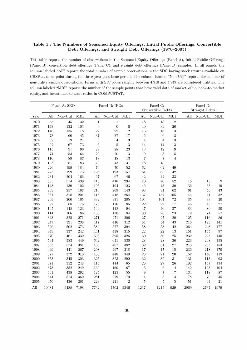
Table 1 : The Numbers of Seasoned Equity Offerings, Initial Public Offerings, ConvertibleDebt Offerings, and Straight Debt Offerings (1970–2005)

This table reports the number of observations in the Seasoned Equity Offerings (Panel A), Initial Public Offerings

(Panel B), convertible debt offerings (Panel C), and straight debt offerings (Panel D) samples. In all panels, the

column labeled “All” reports the total number of sample observations in the SDC having stock returns available on

CRSP at some point during the three-year post-issue period. The column labeled “Non-Util” reports the number of

non-utility sample observations. Firms with SIC codes ranging between 4,910 and 4,949 are considered utilities. The

column labeled “MBI” reports the number of the sample points that have valid data of market value, book-to-market

equity, and investment-to-asset ratios in COMPUSTAT.

Panel A: SEOs Panel B: IPOs Panel C: Panel D:Convertible Debts Straight Debts

Year All Non-Util MBI All Non-Util MBI All Non-Util MBI All Non-Util MBI

1970 55 45 32 1 1 1 18 18 121971 143 132 103 0 0 0 40 39 261972 146 135 118 22 22 12 16 16 131973 73 60 45 37 37 17 6 6 31974 32 19 21 5 4 3 4 4 31975 92 67 73 5 5 3 14 14 131976 115 91 96 28 28 23 13 12 91977 74 53 64 20 20 13 9 8 51978 110 89 87 18 18 13 7 7 41979 103 81 83 43 43 31 18 18 111980 226 199 184 70 70 52 62 62 491981 223 199 173 195 193 157 64 63 421982 234 204 166 67 67 46 42 42 331983 535 514 439 416 416 294 70 70 52 15 13 91984 148 130 102 195 194 123 46 43 30 36 33 191985 269 257 167 210 209 143 93 91 62 61 56 431986 331 318 201 418 418 264 137 137 105 44 41 321987 209 200 165 332 331 205 104 101 72 35 33 201988 97 88 75 178 176 85 22 22 17 46 43 271989 165 148 123 149 148 94 47 46 37 83 80 501990 114 106 86 130 130 84 30 28 23 79 74 571991 343 325 271 271 271 206 27 27 20 125 116 861992 347 321 238 417 416 312 54 54 43 216 195 1411993 526 502 373 580 577 394 58 58 42 264 248 1771994 349 337 242 441 438 315 22 22 13 151 145 971995 470 461 339 395 395 326 30 30 25 232 228 1401996 594 583 449 642 641 530 28 28 26 223 208 1551997 583 574 381 468 467 382 32 31 27 243 233 1531998 449 441 267 298 297 218 17 17 15 236 218 1701999 377 372 313 450 448 349 23 21 20 162 148 1192000 353 345 303 325 323 292 32 32 31 131 113 932001 371 352 248 115 114 65 28 27 26 182 157 1342002 373 352 249 162 160 67 6 6 4 142 123 1042003 461 438 292 125 125 55 9 7 7 134 118 872004 544 514 369 281 279 170 4 3 4 78 70 452005 450 436 261 223 221 2 5 5 5 51 44 21

All 10084 9488 7198 7732 7702 5346 1237 1215 929 2969 2737 1979

30

Table 2 : The Frequency Distribution and the New Issue-to-Asset Ratio of SEOs, IPOs,Convertible Debt Offerings, and Straight Debt Offerings across Size and Book-to-Market

Quintiles (1970–2005)

This table reports the frequency distribution (in percent) and the median new issue-to-asset ratio across size and

book-to-market quintiles for the SEO sample (Panel A), the IPO sample (Panel B), the convertible debt sample

(Panel C), and the straight debt sample (Panel D). In each panel, the left subpanel reports the frequency distribution

defined as the ratio (in percent) of the number of observations in a given size and book-to-market quintile divided by

the total number of observations. In the right subpanel we measure the new issue-to-asset ratio as the proceeds of

new issue obtained from the SDC divided by the book value of assets (COMPUSTAT annual item 6) at the end of

the fiscal year preceding the issue of seasoned equity, convertible debt, and straight debt. Because of data availability

for IPOs, we use the book value of assets at the end of the fiscal year of the issue. We calculate size as the price

per share at the end of June times the number of shares outstanding. We define book equity as stockholder’s equity

(item 216), minus preferred stock, plus balance sheet deferred taxes and investment tax credit (item 35) if available,

minus post-retirement benefit asset (item 330) if available. If stockholder’s equity value is missing, we use common

equity (item 60) plus preferred stock par value (item 130). We measure preferred stock as preferred stock liquidating

value (item 10) or preferred stock redemption value (item 56) or preferred stock par value (item 130) in that order of

availability. If these variables are missing, we use book assets (item 6) minus liabilities (item 181). To calculate the

book-to-market ratio, we use the market size at the end of the fiscal year times the number of shares outstanding.

The breakpoints of size and book-to-market quintiles are from Kenneth French’s website.

Panel A: Frequency distribution, SEOs New issue-to-asset, SEOs

Small 2 3 4 Big All Small 2 3 4 Big

Low 18.92 9.56 5.68 3.59 3.08 40.84 0.893 0.599 0.397 0.235 0.0792 8.30 4.20 3.00 2.10 1.26 18.86 0.449 0.232 0.101 0.068 0.0253 6.69 3.45 2.61 1.65 1.13 15.52 0.281 0.100 0.060 0.040 0.0214 7.21 3.34 2.21 1.38 1.03 15.17 0.174 0.082 0.049 0.027 0.016High 5.73 1.44 1.23 0.69 0.52 9.61 0.139 0.051 0.037 0.017 0.012

All 46.84 21.99 14.73 9.42 7.02 100

Panel B: Frequency distribution, IPOs New issue-to-asset, IPOs

Small 2 3 4 Big All Small 2 3 4 Big

Low 31.90 13.72 6.43 3.05 1.09 56.19 1.748 1.717 1.577 2.251 1.1812 14.11 3.58 1.21 0.47 0.33 19.70 1.151 0.602 0.194 0.266 0.0573 7.72 1.84 0.84 0.40 0.28 11.09 0.835 0.488 0.203 0.216 0.0204 6.09 1.18 0.55 0.31 0.20 8.33 0.835 0.437 0.195 0.083 0.019High 3.60 0.50 0.26 0.22 0.11 4.69 0.828 0.143 0.084 0.040 0.052

All 63.42 20.82 9.30 4.45 2.01 100

Panel C: Frequency distribution, convertible debt issues New issue-to-asset, convertible debt issues

Small 2 3 4 Big All Small 2 3 4 Big

Low 12.12 9.62 7.69 6.15 6.06 41.63 0.672 0.514 0.356 0.243 0.1112 9.81 5.38 3.56 3.27 2.60 24.62 0.429 0.294 0.213 0.101 0.0493 3.94 4.23 2.12 2.88 1.73 14.90 0.377 0.144 0.101 0.072 0.0424 4.42 2.31 1.63 1.54 1.06 10.96 0.188 0.066 0.083 0.048 0.011High 3.46 2.12 1.15 0.58 0.58 7.88 0.191 0.062 0.045 0.039 0.027

All 33.75 23.65 16.15 14.42 12.02 100

Panel D: Frequency distribution, straight debt issues New issue-to-asset, straight debt issues

Small 2 3 4 Big All Small 2 3 4 Big

Low 1.74 1.55 2.11 4.52 12.11 22.03 0.714 0.343 0.256 0.134 0.0692 0.70 1.44 3.63 5.04 10.33 21.14 0.551 0.341 0.252 0.127 0.0433 1.00 2.74 3.81 6.92 8.55 23.03 0.325 0.245 0.135 0.080 0.0244 1.67 3.55 4.48 4.63 7.37 21.70 0.288 0.170 0.082 0.051 0.024High 2.11 2.18 2.11 2.74 2.96 12.11 0.233 0.112 0.067 0.019 0.015

All 7.22 11.48 16.14 23.84 41.32 100

31

Table 3 : Calendar-Time Factor Regressions for the New Issues Portfolio Excess Returns(January 1970–December 2005)

This table reports calendar-time factor regressions for the SEO, IPO, convertible debt, and straight debt portfolio

excess returns. The portfolios consist of firms that have conducted SEOs (Panel A), IPOs (Panel B), convertible

debt offerings (Panel C), or straight debt offerings (Panel D) during the 36 months prior to the month of portfolio

formation. We use two factor models, the CAPM and the Fama and French (1993) three-factor model. We obtain the

factor returns, MKT, SMB, and HML from Kenneth French’s website. We estimate the regressions using Weighted

Least Squares, and compute the t-statistics (in parentheses) using the White (1980) heteroscedasticity-consistent

standard errors.

Panel A: SEOs Panel B: IPOs

Equally-weighted Value-weighted Equally-weighted Value-weighted

CAPM Fama-French CAPM Fama-French CAPM Fama-French CAPM Fama-French

α −0.407 −0.389 −0.435 −0.354 −0.713 −0.429 −0.816 −0.445(−2.43) (−3.52) (−3.76) (−3.04) (−2.60) (−2.18) (−3.03) (−1.91)

MKT 1.291 1.173 1.200 1.145 1.349 1.117 1.438 1.182(34.00) (34.17) (34.19) (29.35) (22.89) (19.46) (21.07) (20.05)

SMB 0.735 0.067 0.908 0.307(10.71) (0.34) (8.41) (3.07)

HML 0.015 −0.118 −0.259 −0.552(0.29) (−1.93) (−2.86) (−4.88)

Panel C: Convertible debt issues Panel D: Straight debt issues

Equally-weighted Value-weighted Equally-weighted Value-weighted

CAPM Fama-French CAPM Fama-French CAPM Fama-French CAPM Fama-French

α −0.631 −0.540 −0.444 −0.257 0.126 −0.261 −0.007 −0.089(−4.20) (−4.72) (−3.38) (−2.00) (0.73) (−2.35) (−0.06) (−0.90)

MKT 1.304 1.199 1.285 1.188 0.877 1.114 0.880 0.978(38.98) (30.91) (42.41) (39.77) (16.01) (33.13) (26.38) (38.17)

SMB 0.707 0.113 0.182 −0.273(8.68) (1.62) (3.48) (−7.77)

HML −0.021 −0.267 0.649 0.128(−0.34) (−4.21) (13.46) (3.17)

32

Table 4 : Calendar-Time Factor Regressions Augmented with the Investment Factor for theNew Issues Portfolio Excess Returns (January 1970–December 2005)

This table reports calendar-time factor regressions augmented with the investor factor for the SEO, IPO, convertible

debt, and straight debt portfolio excess returns. The portfolios consist of firms that have conducted SEOs (Panel

A), IPOs (Panel B), convertible debt offerings (Panel C), or straight debt offerings (panel D) during the 36 months

prior to the month of portfolio formation. We augment the CAPM and the Fama and French (1993) three-factor

model with the investment factor, denoted INV. We construct INV from a triple sort on size, book-to-market, and

investment-to-asset ratio. The investment-to-asset ratio is measured as sum of the annual changes in gross property,

plant and equipment (COMPUSTAT annual item 7) and inventories (item 3) divided by the lagged book value of

assets (item 6). In June of each year, we sort all stocks in ascending order independently on size, book-to-market,

and investment-to-asset, and classify them into three groups, the top 30%, the medium 40%, and the bottom 30%.

We define the investment factor as the average return of the nine low-investment portfolios minus the average return

of the nine high-investment portfolios. The factor returns MKT, SMB, and HML are from Kenneth French’s website.

We estimate the regressions using Weighted Least Squares, and compute the t-statistics (in parentheses) using White

(1980) heteroscedasticity-consistent standard errors. |△α|/|α| denotes the reduction in alphas from the augmented

factor regressions divided by the magnitudes of the alphas from the CAPM and the Fama-French three-factor model

in Table 3.

Panel A: SEOs Panel B: IPOs

Equally-weighted Value-weighted Equally-weighted Value-weighted

CAPM Fama-French CAPM Fama-French CAPM Fama-French CAPM Fama-French

α −0.074 −0.084 −0.139 −0.054 −0.292 −0.052 −0.130 0.205(−0.40) (−0.72) (−1.09) (−0.44) (−0.84) (−0.21) (−0.36) (0.69)

MKT 1.238 1.124 1.153 1.097 1.289 1.062 1.345 1.092(29.29) (33.88) (31.78) (27.84) (19.05) (22.67) (19.39) (18.88)

SMB 0.728 0.059 0.897 0.278(12.75) (1.14) (9.49) (3.46)

HML 0.010 −0.125 −0.268 −0.566(0.22) (−2.21) (−3.06) (−5.33)

INV −0.437 −0.395 −0.384 −0.384 −0.493 −0.437 −0.728 −0.686(−2.74) (−4.78) (−4.73) (−4.99) (−1.80) (−2.55) (−3.04) (−4.13)

|∆α|/|α| 82% 78% 68% 85% 59% 88% 84% −Panel C: Convertible debt issues Panel D: Straight debt issues

Equally-weighted Value-weighted Equally-weighted Value-weighted

CAPM Fama-French CAPM Fama-French CAPM Fama-French CAPM Fama-French

α −0.338 −0.373 −0.202 −0.071 0.458 0.029 0.156 0.056(−2.04) (−3.26) (−1.37) (−0.53) (2.56) (0.27) (1.12) (0.51)

MKT 1.258 1.176 1.247 1.163 0.829 1.069 0.857 0.956(33.94) (31.86) (41.76) (41.92) (14.85) (34.33) (20.95) (36.14)

SMB 0.694 0.100 0.180 −0.273(8.89) (1.52) (4.43) (−9.03)

HML −0.009 −0.256 0.637 0.121(−0.15) (−4.10) (15.07) (3.19)

INV −0.414 −0.250 −0.334 −0.269 −0.378 −0.321 −0.184 −0.159(−3.16) (−2.09) (−3.40) (−2.51) (−3.31) (−5.39) (−1.44) (−2.59)

|∆α|/|α| 46% 31% 55% 72% − 111% − −

33

Table 5 : The Frequency Distribution of New Issues across Investment Deciles

This table reports the frequency distribution of SEOs (Panel A), IPOs (Panel B), convertible debt offerings (Panel C), and straight debt offerings (Panel D)

across investment-to-asset deciles. The frequency distribution is defined as the ratio of the number of observations in a given investment-to-asset decile divided

by the total number of observations. We measure assets as the book value of assets (COMPUSTAT annual item 6) and investment as the sum of changes in gross

property, plant, and equipment (item 7) and inventories (item 3). We sort nonissuing firms in June of each year by their investment-to-asset ratios to obtain the

decile breakpoints, and then assign each issuer to one of the investment-to-asset deciles.

Low 2 3 4 5 6 7 8 9 High

Panel A: SEOs

7.80% 7.24% 7.78% 7.52% 8.35% 8.74% 9.97% 11.13% 14.01% 17.47%

Panel B: IPOs

5.45% 3.18% 4.32% 3.86% 3.41% 2.73% 4.09% 5.45% 6.82% 60.68%

Panel C: Convertible debt offerings

4.86% 4.86% 6.21% 6.34% 8.77% 10.39% 10.80% 14.44% 17.41% 15.92%

Panel D: Straight debt offerings

8.36% 9.32% 9.86% 10.93% 13.20% 11.65% 10.45% 9.86% 6.87% 9.50%

34

Table 6 : Calendar-Time Factor Regressions of the Composite Issuance Zero-InvestmentPortfolio Returns, with and without the Investment Factor (January 1970 to December 2005)

This table reports calendar-time factor regressions of the composite issuance zero-investment portfolio returns. In

Panel A, we follow Daniel and Titman (2006) and define the composite issuance measure of equity for a firm in year

t, denoted ι(t− τ, t), as the growth in the market value of its equity that is not attributable to its stock returns from

year t− τ to year t: ι(t− τ, t)=log (MEt/MEt−τ )− r(t− τ, t) where r(t− τ, t) is the stock return from year t− τ to

t, adjusted for stock splits and stock dividends, and MEt is the market value of equity at year t. As in Daniel and

Titman, we use τ =5. In Panel B, we define the composite issuance measure of debt as the growth in the book value

of debt: ιD(t − τ )= log (BDt/BDt−τ ), where BDt−τ is the book value of debt. Similar to the composite issuance of

equity, τ =5. In June of year t, we match returns from July of year t to June of year t+1 with the composite issuance

measures determined at the fiscal yearend in calendar year t−1. We then sort firms into deciles each month based

on their composite issuance measures. The composite issuance zero-investment portfolio returns are defined as the

average high composite issuance (highest three deciles) portfolio returns minus the average low composite issuance

(lowest three deciles) portfolio returns. We estimate the regressions using Weighted Least Squares, and calculate the

t-statistics (in parentheses) using the White (1980) heteroscedasticity-consistent standard errors.

Panel A: Composite issuance of equity Panel B: Composite issuance of debt

Equally-weighted Value-weighted Equally-weighted Value-weighted

CAPM Fama-French CAPM Fama-French CAPM Fama-French CAPM Fama-French

α −0.558 −0.367 −0.590 −0.359 −0.532 −0.551 −0.309 −0.265(−4.38) (−4.45) (−4.94) (−3.57) (−8.59) (−8.31) (−2.80) (−2.34)

MKT 0.435 0.235 0.348 0.187 0.150 0.157 0.105 0.083(15.25) (9.00) (12.13) (6.19) (10.49) (8.34) (3.90) (2.67)

SMB 0.400 0.156 0.010 −0.004(9.76) (3.23) (0.29) (−0.10)

HML −0.383 −0.404 0.029 −0.071(−10.78) (−9.20) (0.92) (−1.33)

Equally-weighted Value-weighted Equally-weighted Value-weighted

CAPM Fama-French CAPM Fama-French CAPM Fama-French CAPM Fama-French

α −0.399 −0.240 −0.364 −0.156 −0.357 −0.377 −0.180 −0.139(−3.18) (−3.08) (−2.93) (−1.49) (−5.73) (−5.91) (−1.47) (−1.14)

MKT 0.408 0.212 0.307 0.151 0.118 0.127 0.082 0.061(10.69) (8.48) (9.09) (5.07) (8.18) (8.16) (2.98) (2.79)

SMB 0.398 0.153 0.007 −0.007(9.55) (3.50) (0.27) (−0.15)

HML −0.380 −0.400 0.033 −0.067(−10.87) (−9.50) (1.30) (−1.25)

INV −0.234 −0.189 −0.333 −0.302 −0.264 −0.265 −0.196 −0.192(−1.82) (−3.00) (−3.09) (−5.16) (−5.55) (−5.66) (−2.23) (−2.22)

|∆α|/|α| 28% 35% 38% 57% 33% 32% 42% 48%

35

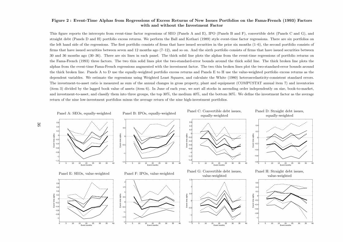
Figure 2 : Event-Time Alphas from Regressions of Excess Returns of New Issues Portfolios on the Fama-French (1993) Factorswith and without the Investment Factor

This figure reports the intercepts from event-time factor regressions of SEO (Panels A and E), IPO (Panels B and F), convertible debt (Panels C and G), and

straight debt (Panels D and H) portfolio excess returns. We perform the Ball and Kothari (1989) style event-time factor regressions. There are six portfolios on

the left hand side of the regressions. The first portfolio consists of firms that have issued securities in the prior six months (1–6), the second portfolio consists of

firms that have issued securities between seven and 12 months ago (7–12), and so on. And the sixth portfolio consists of firms that have issued securities between

30 and 36 months ago (30–36). There are six lines in each panel. The thick solid line plots the alphas from the event-time regressions of portfolio returns on

the Fama-French (1993) three factors. The two thin solid lines plot the two-standard-error bounds around the thick solid line. The thick broken line plots the

alphas from the event-time Fama-French regressions augmented with the investment factor. The two thin broken lines plot the two-standard-error bounds around

the thick broken line. Panels A to D use the equally-weighted portfolio excess returns and Panels E to H use the value-weighted portfolio excess returns as the

dependent variables. We estimate the regressions using Weighted Least Squares, and calculate the White (1980) heteroscedasticity-consistent standard errors.

The investment-to-asset ratio is measured as sum of the annual changes in gross property, plant and equipment (COMPUSTAT annual item 7) and inventories

(item 3) divided by the lagged book value of assets (item 6). In June of each year, we sort all stocks in ascending order independently on size, book-to-market,

and investment-to-asset, and classify them into three groups, the top 30%, the medium 40%, and the bottom 30%. We define the investment factor as the average

return of the nine low-investment portfolios minus the average return of the nine high-investment portfolios.

Panel A: SEOs, equally-weighted Panel B: IPOs, equally-weightedPanel C: Convertible debt issues,

equally-weightedPanel D: Straight debt issues,

equally-weighted

0 5 10 15 20 25 30 35 40−1.2

−1

−0.8

−0.6

−0.4

−0.2

0

0.2

0.4

0.6

Event months

Eve

nt−

time

alph

a

0 5 10 15 20 25 30 35 40−1.5

−1

−0.5

0

0.5

1

Event months

Eve

nt−

time

alph

a

0 5 10 15 20 25 30 35 40

−1.4

−1.2

−1

−0.8

−0.6

−0.4

−0.2

0

0.2

0.4

0.6

Event months

Eve

nt−

time

alph

a

0 5 10 15 20 25 30 35 40−0.8

−0.6

−0.4

−0.2

0

0.2

0.4

Event months

Eve

nt−

time

alph

a

Panel E: SEOs, value-weighted Panel F: IPOs, value-weightedPanel G: Convertible debt issues,

value-weightedPanel H: Straight debt issues,

value-weighted

0 5 10 15 20 25 30 35 40

−1

−0.8

−0.6

−0.4

−0.2

0

0.2

0.4

0.6

0.8

1

Event months

Eve

nt−

time

alph

a

0 5 10 15 20 25 30 35 40−2

−1.5

−1

−0.5

0

0.5

1

1.5

2

Event months

Eve

nt−

time

alph

a

0 5 10 15 20 25 30 35 40−1.5

−1

−0.5

0

0.5

1

1.5

Event months

Eve

nt−

time

alph

a

0 5 10 15 20 25 30 35 40

−1

−0.8

−0.6

−0.4

−0.2

0

0.2

0.4

0.6

Event months

Eve

nt−

time

alph

a

36

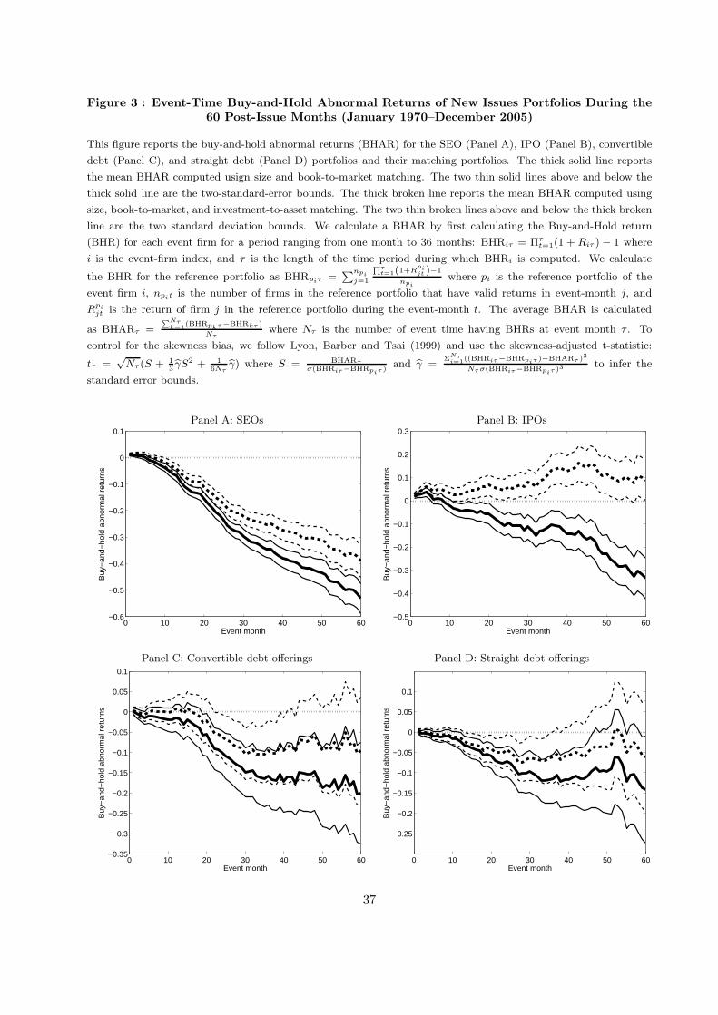
Figure 3 : Event-Time Buy-and-Hold Abnormal Returns of New Issues Portfolios During the60 Post-Issue Months (January 1970–December 2005)

This figure reports the buy-and-hold abnormal returns (BHAR) for the SEO (Panel A), IPO (Panel B), convertible

debt (Panel C), and straight debt (Panel D) portfolios and their matching portfolios. The thick solid line reports

the mean BHAR computed usign size and book-to-market matching. The two thin solid lines above and below the

thick solid line are the two-standard-error bounds. The thick broken line reports the mean BHAR computed using

size, book-to-market, and investment-to-asset matching. The two thin broken lines above and below the thick broken

line are the two standard deviation bounds. We calculate a BHAR by first calculating the Buy-and-Hold return

(BHR) for each event firm for a period ranging from one month to 36 months: BHRiτ = Πτt=1(1 + Riτ ) − 1 where

i is the event-firm index, and τ is the length of the time period during which BHRi is computed. We calculate

the BHR for the reference portfolio as BHRpiτ =Pnpi

j=1

Qτt=1(1+R

pijt )−1

npiwhere pi is the reference portfolio of the

event firm i, npit is the number of firms in the reference portfolio that have valid returns in event-month j, and

Rpijt is the return of firm j in the reference portfolio during the event-month t. The average BHAR is calculated

as BHARτ =PNτ

k=1(BHRpkτ−BHRkτ )

Nτwhere Nτ is the number of event time having BHRs at event month τ . To

control for the skewness bias, we follow Lyon, Barber and Tsai (1999) and use the skewness-adjusted t-statistic:

tτ =√

Nτ (S + 13

bγS2 + 16Nτ

bγ) where S = BHARτ

σ(BHRiτ−BHRpiτ )and bγ =

ΣNτi=1

((BHRiτ−BHRpiτ )−BHARτ )3

Nτ σ(BHRiτ−BHRpiτ )3to infer the

standard error bounds.

Panel A: SEOs Panel B: IPOs

0 10 20 30 40 50 60−0.6

−0.5

−0.4

−0.3

−0.2

−0.1

0

0.1

Event month

Buy

−an

d−ho

ld a

bnor

mal

ret

urns

0 10 20 30 40 50 60−0.5

−0.4

−0.3

−0.2

−0.1

0

0.1

0.2

0.3

Event month

Buy

−an

d−ho

ld a

bnor

mal

ret

urns

Panel C: Convertible debt offerings Panel D: Straight debt offerings

0 10 20 30 40 50 60−0.35

−0.3

−0.25

−0.2

−0.15

−0.1

−0.05

0

0.05

0.1

Event month

Buy

−an

d−ho

ld a

bnor

mal

ret

urns

0 10 20 30 40 50 60

−0.25

−0.2

−0.15

−0.1

−0.05

0

0.05

0.1

Event month

Buy

−an

d−ho

ld a

bnor

mal

ret

urns

37

Figure 4 : Event-Time Evolution of Investment-to-Asset of Issuers and Matching NonissuersDuring the 60 Post-Issue Months (January 1970 to December 2005)

This figure plots issuers’ and matching nonissuers’ median investment-to-asset ratios during the 60 months after

SEOs (Panel A), IPOs (Panel B), convertible debt issues (Panel C), and straight debt issues (Panel D). Month zero

is the offering month. The investment-to-asset ratio is measured as sum of the annual changes in gross property,

plant and equipment (COMPUSTAT annual item 7) and inventories (item 3) divided by the lagged book value of

assets (item 6). The solid lines are for issuers and the broken lines are for matching nonissuers. We use the following

matching procedure. For a given panel, say Panel A for the SEO sample, we sort all the firms that have not issued

seasoned equity within the prior 36 months on their size and book-to-market equity in June of each year to form 25

size and book-to-market portfolios of nonissuers. For each SEO firm, we use the size and book-to-market breakpoints

to identify its matching portfolio. The matching portfolio’s median investment-to-asset ratio is compared with that

of the issuer.

Panel A: SEOs Panel B: IPOs

0 10 20 30 40 50 600

0.02

0.04

0.06

0.08

0.1

0.12

0.14

0.16

Event month

Inve

stm

ent−

to−

asse

t

0 10 20 30 40 50 600

0.2

0.4

0.6

0.8

1

1.2

1.4

Event month

Inve

stm

ent−

to−

asse

t

Panel C: Convertible debt offerings Panel D: Straight debt offerings

0 10 20 30 40 50 600

0.02

0.04

0.06

0.08

0.1

0.12

0.14

0.16

0.18

0.2

Event month

Inve

stm

ent−

to−

asse

t

0 10 20 30 40 50 600

0.02

0.04

0.06

0.08

0.1

0.12

0.14

0.16

Event month

Inve

stm

ent−

to−

asse

t

38

Figure 5 : Event-Time Evolution of Profitability of Issuers and Matching Nonissuers Duringthe Post-Issue 60 Months (January 1970 to December 2005)

This figure plots issuers’ and matching nonissuers’ median profitability during the 60 months after SEOs (Panel A),

IPOs (Panel B), convertible debt issues (Panel C), and straight debt issues (Panel D). Month zero is the offering

month. We measure profitability as net income before extraordinary items (item 18) divided by lagged book value of

equity. We define book equity as stockholder’s equity (item 216), minus preferred stock, plus balance sheet deferred

taxes and investment tax credit (item 35) if available, minus post-retirement benefit asset (item 330) if available.

If stockholder’s equity is missing, we use common equity (item 60) plus preferred stock par value (item 130). We

measure preferred stock as preferred stock liquidating value (item 10) or preferred stock redemption value (item 56)

or preferred stock par value (item 130) in that order of availability. If these variables are missing, we use book assets

(item 6) minus liabilities (item 181). The solid lines are for issuers and the broken lines are for matching nonissuers.

We use the following matching procedure. For a given panel, say Panel C for the convertible debt sample, we sort all

the firms that have not issued convertible debts within the prior 36 months on their size and book-to-market equity in

June of each year to form 25 size and book-to-market portfolios of nonissuers. For each firm issuing convertible debt,

we then use the size and book-to-market breakpoints to identify its matching portfolio. The matching portfolio’s

median profitability is compared with that of the issuer.

Panel A: SEOs Panel B: IPOs

0 10 20 30 40 50 600

0.02

0.04

0.06

0.08

0.1

0.12

0.14

0.16

Event month

Pro

fitab

ility

0 10 20 30 40 50 600

0.2

0.4

0.6

0.8

1

1.2

Event month

Pro

fitab

ility

Panel C: Convertible debt offerings Panel D: Straight debt offerings

0 10 20 30 40 50 600

0.02

0.04

0.06

0.08

0.1

0.12

0.14

0.16

0.18

0.2

Event month

Pro

fitab

ility

0 10 20 30 40 50 600

0.02

0.04

0.06

0.08

0.1

0.12

0.14

0.16

Event month

Pro

fitab

ility

39

Figure 6 : Event-Time Evolution of Investment-to-Asset of High Composite Issuance Firms(Top 30%) and Low Composite Issuance Firms (Bottom 30%) During the 11 years around

Portfolio Formation (January 1970 to December 2005)

This figure plots the median investment-to-asset ratios and high composite issuance firms (top 30%, the solid line)

and low composite issuance firms (bottom 30%, the broken line) during the 11 years around portfolio formation.

Year zero is the year of portfolio formation. In Panel A, we form ten portfolios in each June by sorting on Daniel

and Titman’s (2006) composite equity issuance measure and record the monthly returns from July to next June. For

firm i in year t, the composite equity issuance measure is the growth in the market equity not attributable to stock

returns: ιi(t − τ, t) = log(MEit/MEit−τ ) − ri(t − τ, t), where MEit is the market equity at year t and ri(t − τ, t) is

the stock return from year t− τ to year t. The composite debt issuance is defined as the growth in the book value of

debt, denoted BD. BD is measured as the sum of long-term debt (COMPUSTAT annual item 9) and debt in current

liabilities (item 34). For firm i in year t, ιiD(t − τ, t) = log (BDit/BDit−τ ). In constructing the composite issuance

variables for both equity and debt, we set τ = 5. We measure investment-to-asset as the annual change in gross

property, plant, and equipment (item 7) plus the annual change in inventories (item 3) divided by the lagged book

value of assets (item 6).

Panel A: Composite equity issuance Panel B: Composite debt issuance

−6 −4 −2 0 2 4 60.06

0.07

0.08

0.09

0.1

0.11

0.12

0.13

Event year

Inve

stm

ent−

to−

asse

t

−6 −4 −2 0 2 4 60.06

0.07

0.08

0.09

0.1

0.11

0.12

0.13

0.14

Event year

Inve

stm

ent−

to−

asse

t

40