Jim Been and Marike Knoef

The Necessity of Self-Employment Towards Retirement Evidence from Labor Market Dynamics and Search Requirements for Unemployment Benefits

DP 04/2015-009

The necessity of self-employment towards retirement:evidence from labor market dynamics and search

requirements for unemployment benefits ∗

Jim Been † Marike Knoef ‡

April 2015

Abstract

This paper investigates whether individuals at the end of working life choose self-employment

out of necessity and to what degree job search requirements for unemployment benefits induce

people to become self-employed. For this purpose we analyze labor market transitions for peo-

ple between the ages of 50 and 63 using a dynamic multinomial logit model with unobserved

heterogeneity.

The results indicate that at the end of the career individuals with a weak labor market posi-

tion have a relatively high probability to become self-employed, e.g. to end or avoid a period

of unemployment or inactivity (necessity driven self-employment). Contrasting some earlier

work, the results do not suggest that self-employment is used as a gradual retirement route for

employees. A difference-in-differences analysis shows that job search requirements among un-

∗Financial support has been provided by Instituut Gak and Netspar. We would like to thank the participants ofthe HSZ Lunch Seminar Series at the Leiden University Department of Economics, the SMYE 2012 Mannheim,the CPB Research Seminar 2012 at the Netherlands Bureau for Economic Policy Analysis (CPB), the ESPE 2012Bern, the IIPF 2012 Dresden, the Netspar IPW 2013 Amsterdam, the IZA Workshop on Labor Markets and La-bor Market Policies for Older Workers 2013 Bonn, the 16th IZA European Summer School in Labor Economics2013 Buch am Ammersee, the EEA conference 2013 Gothenburg and the Netspar Pension Day 2013 Utrecht.More particularly, we are indebted to our colleagues at the Leiden University Department of Economics as well asEmre Akgunduz, Rob Alessie, Hans Bloemen, Pierre Cahuc, Amelie Constant, Kathrin Degen, Karina Doorley,Rob Euwals, T. Scott Findley, Didier Fouarge, Daniel Harenberg, Stefan Hochguertel, Jens Hogenacker, Adri-aan Kalwij, Mauro Mastrogiacomo, Raymond Montizaan, Tuomas Pekkarinen, Sophia Rabe-Hesketh, MarcelloSartarelli, Eva Sierminska, Jan-Maarten van Sonsbeek, Konstantinos Tatsiramos, Nicole Voskuilen-Bosch, Danielvan Vuuren, Michele Weynandt and Jeffrey Wooldridge.

†Department of Economics at Leiden University and Netspar. Corresponding address: Department of Eco-nomics, Leiden University, PO Box 9520, Steenschuur 25, 2300 RA Leiden, the Netherlands. Tel.: +31 71 5278569. (e-mail address: j.been@law.leidenuniv.nl)

‡Department of Economics at Leiden University and Netspar (e-mail address: m.g.knoef@law.leidenuniv.nl)

employed older workers increased the outflow from unemployment and decreased the inflow

into unemployment, but did not increase self-employment out of necessity or opportunity.

JEL codes: C23, J14, J26, J64, J68

Keywords: Labor market dynamics, retirement, self-employment, unemployment insurance,

job search requirements.

2

1 Introduction

In virtually all OECD countries, labor force participation rates of the 50+ population decreased

in the period from the 1960s to the mid-1990s (OECD, 2011). This was partially due to gen-

erous unemployment insurance, disability insurance and early retirement schemes (Gruber &

Wise, 1998).1 Since the mid-1990s aging has raised concerns about the sustainability of the

welfare state and reforms have been undertaken to increase the labor force participation of the

50+ population. As a result, the share of people in paid-employment2 and self-employment

increased. This paper focuses on self-employment at older ages and the introduction of job

search requirements for unemployed older workers.

This paper’s contribution to the literature is twofold. To begin with, this study contributes

to the literature on the importance of necessity and opportunity driven self-employment. In

the literature, two main hypotheses have risen to explain self-employment at older ages. First,

self-employment may be chosen out of necessity, to end or to avoid unemployment.3 The

50+ population particularly faces difficulties finding a new job once unemployed (Chan &

Stevens, 2001 and Maestas & Li, 2006). Second, self-employment may be chosen as an op-

portunity to reduce working hours and enhance gradual retirement.4 To investigate the nature

of self-employment at older ages we test 1) whether transitions from unemployment to self-

employment are important and increase with age5, 2) whether high unemployment rates push

workers from paid-employment to self-employment6, and 3) whether the introduction of job

1Country-specific analyses can be found in Bould (1980), Hogarth (1988), Ruhm (1995), Riphahn (1997),Kerkhofs et al. (1999), Hernoes et al. (2000), Roed & Haugen (2003), Friedberg & Webb (2005), Van Vuuren &Van Vuren (2007), Euwals & Van Vuuren (2010), Euwals et al. (2012) and De Vos et al. (2012).

2Defined as being an employee.3E.g. Taylor (1999), Reize (2000), Earle & Sakova (2000), Kuhn & Schuetze (2001), Kellard et al. (2002),

Rissman (2003) and Glocker & Steiner (2007).4This is suggested by Fuchs (1982), Hurd (1996), Bruce et al. (2000), Morris & Mallier (2003), Zissimopoulos

& Karoly (2007), Giandrea et al. (2008), and Gu (2009). Hamilton (2000) finds that nonpecuniary benefits ofself-employment, such as the flexibility in working hours decisions, are an important reason to choose for self-employment.

5Parker & Rougier (2007) find that transitions from unemployment to self-employment are relatively impor-tant and argue that this indicates necessity-driven self-employment at older ages.

6Several studies find that high unemployment rates increase self-employment propensities, e.g. Benedict &Hakobyan (2008), Kim & Cho (2009), and Congregado et al. (2012). This latter effect is known as the recessionpush hypothesis. This hypothesis is, however, not confirmed in all papers (Moore & Mueller, 2002 and Tapia,2008). Among others, Carrasco (1999) finds that self-employment becomes more attractive when the economicsituation improves (the prosperity pull hypothesis).

3

search requirements for unemployed older workers increases self-employment. For the last test

we use a Dutch UI reform which introduced job search requirements for unemployed persons

between the age of 57.5 and 63 as from January 2004. Before this reform unemployed older

workers did not have to search for a job in order to receive unemployment benefits. The re-

form implied an exogenous and unanticipated shock in the attractiveness of unemployment as

a pathway to retirement. Whereas Lammers et al. (2013) and Hullegie & Van Ours (2013)

investigate the effect of this reform on the outflow from welfare and substitution effect with

regard to disability and early retirement7, we focus on substitution between unemployment and

self-employment. Self-employment may increase when unemployment becomes less attractive

as an exit route to retirement. As far as we know, there are no other studies that investigated the

effect of job search requirements on substitution between unemployment and self-employment

as an exit route to retirement.8

Our second contribution concerns the effect of job search requirements on the inflow to

unemployment. We expect that the introduction of search requirements for unemployed older

workers lowers the inflow into unemployment, since job search requirements make unemploy-

ment a less attractive exit route to retirement. Other studies that investigate the inflow into

unemployment are focused on entrance requirements to unemployment insurance (e.g. Green

& Riddell, 1997, Christofides & McKenna, 1996) and on the level and/or duration of benefits

(e.g. Andersen & Meyer, 1997, Winter-Ebmer, 2003, Lalive et al., 2006, and Tuit & Van Ours,

2010). Lalive et al. and Tuit et al., for example, focus on unemployed older workers and show

that benefit duration affects the inflow to unemployment insurance. The bulk of the literature

on search requirements is focused on the effects of exiting unemployment instead of the inflow

to unemployment (Fredriksson & Holmlund, 2006).

This paper analyzes labor market transitions using a dynamic multinomial logit model.9

This model allows us to study the pathways through which people enter self-employment, to

7Lammers et al. (2013) and Hullegie & Van Ours (2013) both find that the 2004 UI reform significantlyincreased exits from unemployment to paid-employment. Lammers et al. (2013) also find substitution effectsbetween unemployment insurance and disability insurance.

8For an overview of the literature regarding the effects of job search requirements in unemployment, seeFredriksson & Holmlund (2006).

9Among others, this model has been used by Cappellari et al. (2010), Constant & Zimmerman (2004),Caliendo & Uhlendorff (2008) and Martinez-Granado (2002).

4

study the effect of the unemployment rate on transitions to self-employment, and to study

the effect of the introduction of job search requirements on labor market transitions using a

difference-in-differences approach. We correct for unobserved heterogeneity by allowing for

correlated random effects (Wooldridge, 2010) and we take into account the initial conditions

problem by using the method of Wooldridge (2005). Estimating a dynamic multinomial logit

model avoids a possible sample selection bias, which may occur when considering binomial

models describing transition processes. To estimate the model, the paper takes advantage of

the long panel dimension of the Dutch Income Panel data (1989-2009).

Our main finding is that at the end of the career unemployed individuals have a relatively

high probability to enter self-employment (necessity driven) and this effect is found to be signif-

icantly increasing with age. For men in paid-employment the results show significant evidence

for the recession push hypothesis. For inactive men, on the other hand, we find that a higher un-

employment rate decreases the probability to enter self-employment. For women we find that

a higher unemployment rate decreases the probability of entering self-employment regardless

of the previous labor market status. Introducing job search requirements for the unemployed at

the end of their working life increased exits from unemployment and reduced the inflow to un-

employment. This reform, however, did not increase self-employment out of necessity (we find

no significant increase in flows from unemployment to self-employment due to the reform).

The structure of the paper is as follows. The next section describes the Dutch unemploy-

ment insurance system. Section 3 presents the model, and section 4 describes the data. Sec-

tion 5 reports the estimation results, after which section 6 provides some discussion and sec-

tion 7 concludes the paper.

2 Unemployment insurance towards retirement

As this paper focuses on self-employment and unemployment as exit routes to retirement, this

section provides an overview of the Dutch UI benefit system. In the 1990s unemployment was

an attractive exit route for older workers because of generous arrangements and easy eligibility

5

rules. As from the age of 57.5 people had the possibility to use UI benefits up to the manda-

tory retirement age without having to search for a job. Unemployment was, therefore, used

frequently as an exit route to retirement. The number of UI beneficiaries expanded and, in light

of the aging population, reforms have been undertaken.10

This paper investigates the effect of a UI reform introduced on January 1st 2004, which

implied that unemployed persons older than 57.5 years were no longer exempted from the

requirement to search actively for a job. Search requirements involve that persons in unem-

ployment 1) have a mandatory intake meeting at the unemployment office, where individual

criteria are made regarding the expected activities undertaken during unemployment that are

ex post testable,11 2) have the obligation to accept suitable job-offers, where suitable job offers

are defined by the educational level and the time spent in unemployment, 3) have to make a

sufficient number of applications,12 where sufficiency is individually determined and related to

the labor market, the number of available vacancies and personal health, 4) have to participate

in educational programs and job search assistance when they are assumed to not to be able to

find work within six months, and 5) have regular report meetings every 4-6 weeks in addition

to the mandatory intake meeting and the follow-up to explain the further procedures.

The baseline from which individual arrangements are made is the requirement of applying

for a job once a week on average. An automatic exception is made for individuals starting

their own business. Furthermore, exceptions are made for persons participating in care or

volunteering for at least 20 hours per week for a period of at most six months, individuals

taking part in an educational program, people of age 64, or persons older than 62 years and 2

months who already received UI benefits for at least a year in 2004. The first two exceptions

are made because they may increase the probability to find a job. The latter two exceptions

are made because of a transitory regime. The strictness of job monitoring in the Netherlands is

high13 and due to the risk of substantial financial sanctions we can reasonably assume people

10For an international comparison of unemployment as an early retirement route, see Gruber & Wise (1998).11The employability of an individual is determined by objective characteristics such as profession, education,

age and experience as well as the subjective impression of the caseworker during the interview.12The following options are considered to be an application: letter, e-mail, phone call or nuncupative contact

with a company, registering at an agency, having a job interview and doing an assessment.13From an international perspective, Venn (2012) ranks the Netherlands among countries with a high strictness

of job search monitoring. The OECD indicator suggests that monitoring job search is stricter in the Netherlands

6

to be complying with the search requirements (Verveen et al., 2005). After some time, people

even have to accept all job offers irrespective of their educational level.

Fulfilling above mentioned requirements, together with eligibility requirements that people

have worked at least 26-out-of-36 weeks, gives persons the right to receive UI benefits. Until

October 2006 the maximum UI benefits duration for receiving 70% of previous earnings was

age-dependent and amounted to a maximum of 42, 48 and 60 months for persons aged 50-54,

55-59 and 60-64 respectively. Until August 2003 persons aged 57.5+ could, in principal, even

extend the benefit period up to the age of 65 by using extended UI benefits. These extended

UI benefits amounted 70% of minimum wage. From August 2003, extended UI benefits were

abolished simultaneously with the introduction of the so called IOAW-benefits14 targeted at

unemployed 50+ individuals. The only difference between the extended UI benefits and the

IOAW for older unemployed is that receiving the latter depends on the income of the spouse

while extended benefits were unconditional on the income of the spouse. Single households

are therefore indifferent between receiving extended UI benefits or IOAW benefits.

In October 2006, both benefits and the duration of benefits were moderated for all UI recip-

ients and the maximum UI benefit duration was made conditional on the employment history,

with a maximum of 38 months. However, after 38 months of UI benefits, unemployed elderly

can obtain social benefits from IOAW and the IOW15 (implemented in 2004 and 2009, respec-

tively) to complement household income up to subsistence level without asset-based means

testing (and for the IOW also unconditional on the income of a partner). Furthermore, self-

employed elderly individuals with a low income who have to stop their business can receive

benefits to complement their income up to subsistence level, without the strict asset-based

means testing from social assistance benefits.16

than in countries such as the US, Canada and Scandinavian countries.14Wet inkomensvoorziening oudere en gedeeltelijk arbeidsongeschikte werkloze werknemers.15Inkomensvoorziening oudere werklozen.16This program is called the IOAZ (Wet Inkomensvoorziening oudere en gedeeltelijk arbeidsongeschikte

gewezen zelfstandigen.)

7

3 Model

3.1 Exit routes to retirement

This section describes the model we use to investigate labor market transitions among the 50+

population. The exit route to retirement can be seen as the outcome of a maximization pro-

cess, in which individuals reevaluate their optimal labor market status each period, given their

preferences and the constraints that coincide with each labor market state. Individuals compare

utility streams associated with different exit routes and choose the alternative with the highest

utility stream. More specifically, we define the inter-temporal utility of individual i as follows:

Uit =T

∑τ=t

(1+ρ)t−τuτ(ciτ, liτ, jiτ;siτ,viτ) (1)

where ciτ and liτ denote consumption and leisure of individual i in time period τ implicitly

defined by labor market state j. ρ is the discount factor and T the time horizon of the in-

dividual. In our model we distinguish between four mutually exclusive labor market states:

paid-employment ( j = 1), self-employment ( j = 2), unemployment insurance ( j = 3), and

inactivity ( j = 4).17 Each labor market status is associated with it’s own consumption and

leisure possibilities, but labor market status itself may also influence the utility function di-

rectly. E.g., conditional on leisure and consumption, some people receive a higher utility from

self-employment than from paid-employment, due to characteristics of self-employment such

as the independence and flexibility that self-employment provides.

Social insurance rules siτ that hold for individual i in period τ influence the exit route to

retirement. An increase of job search requirements, for example, decreases the amount of

leisure and so the value of unemployment as a retirement route. Furthermore, transitions from

self-employment or inactivity to unemployment are not possible because only persons in paid-

employment are eligible for UI benefits. Finally, observed and unobserved characteristics viτ

influence the utility function indirectly through preferences. For example, age, the number of

children in the household, and education may influence the utility perceived from consumption

17Inactivity includes individuals in disability, welfare, early retirement, and individuals without personal in-come.

8

and leisure.

Equation 1 provides a guideline for the empirical specification of the model. It shows that

individuals choose the exit route that maximizes their utility over consumption, leisure, and

labor market status. Furthermore, individual characteristics and social insurance rules affect

current and future labor market statuses. For the empirical implementation of the problem,

like Blau (1998) and Mastrogiacomo et al. (2004), we approximate the value function Uit for

individual i who chooses labor market status j at time t with a linear function:

Vi j(t) = Xitβ j +Zit−1⊗ [1 AGE ′it Y EAR′it ]γ j +Zit−1URtθ j +Di jt +µi j + εi jt , (2)

where Xit is a vector of observed personal and household characteristics that influence prefer-

ences as shown in (1). Zit−1 is a vector of dummy variables indicating lagged labor market

status. AGEit and Y EARit are vectors of dummy variables indicating age and year categories.

These are interacted with Zit−1 to allow for mobility differences across age and periods. URt

is the unemployment rate in period t, which we interact with Zit−1 to take into account that

the unemployment rate may affect individuals with various previous employment states differ-

ently. The treatment variables function D contains variables and interactions that we use to

identify the effect of the job search requirements introduced in 2004 and will be explained in

section 3.2.

Finally, the terms µi j describe individual specific unobserved heterogeneity and εi jt are i.i.d.

error terms, which we assume to be independent of the explanatory variables and to follow a

Type I extreme value distribution. Hence, the probability for individual i to have labor market

status j at time t > 0 can be written as

P( jt |Xit ,Zit−1,AGEit ,Y EARi,t ,URt ,Di jt ,µi1, ...,µiJ) =

exp(Xitβ j +Zit−1⊗ [1 AGE ′it Y EAR′it ]γ j +Zit−1URtθ j +Di jt +µi j)

∑Jk=1 exp(Xitβk +Zit−1⊗ [1 AGE ′it Y EAR′it ]γk +Zit−1URtθk +Dikt +µik)

, (3)

where J denotes the number of mutually exclusive labor market states distinguished in the

model. To identify the model, β1,γ1,θ1 and µi1 are normalized to zero (paid-employment is

9

the reference category). The unobserved heterogeneity or random effects µi = (µi2,µi3,µi4)′ are

assumed to follow a multivariate normal distribution with mean zero and variance Σµ.

Introducing unobserved heterogeneity has the advantage that the irrelevance of independent

alternatives (IIA) property of the multinomial logit model is avoided. Furthermore, allowing for

unobserved heterogeneity within choice possibilities will give true, instead of spurious, state

dependence in the model. The initial labor market status Zi0 is not fixed or exogenous and, as

in most papers, we do not have the entire history of the process generating individual’s employ-

ment dynamics available. Therefore, the initial conditions problem arises, which is discussed

by Heckman (1981). To deal with this problem Heckman (1981) proposed to estimate a static

multinomial logit model for the initial state with different slope parameters and without lagged

labor market status, simultaneously with the dynamic model. Several studies investigating

transitions between multiple states have used this method, e.g. Gong et al. (2000), Uhlendorff

(2006) and Cappellari et al. (2010). In this paper we will use an alternative approach, proposed

by Wooldridge (2005), to take into account the initial conditions problem. In the method of

Wooldridge (2005), individual specific heterogeneity terms are modeled conditional on the ini-

tial condition, the initial value of the lagged dependent variable, and the individual mean of

time-varying covariates

µi j = Zi0α1 j +Xiα2 j +ai j j = 2,3,4 (4)

where Zi0 is the vector of initial conditions and Xi the vector of the individual mean of time-

varying covariates. The remaining stochastic element, ai j, is assumed to follow a multivariate

normal distribution with mean zero and variance Σa. In other words,

ai2

ai3

ai4

= L

ηi2

ηi3

ηi4

with

ηi2

ηi3

ηi4

∼ N

0

0

0

,

1 0 0

0 1 0

0 0 1

, (5)

where L is the Cholesky matrix of Σa which has to be estimated (the unique lower triangular

matrix such that LL′ = Σa). In this way, we allow for unobserved heterogeneity within and

10

between choice possibilities.

Applying the Wooldridge correction for initial conditions in the way explained above, au-

tomatically results in a Correlated Random Effects model (Mundlak, 1978). Applying this

Correlated Random Effects regression has the advantage of allowing for correlation between

observed- and unobserved heterogeneity similar to a fixed effects model, even in an unbalanced

panel (Wooldridge, 2010).

Akay (2012) studied the performance of the Wooldridge method, compared to the Heck-

man method. He found that the method proposed by Wooldridge works well for moderately

long panels (5-8 periods) and that all methods perform equally well for panels of long dura-

tion (longer than 15-20 periods)18. For short panels, Rabe-Hesketh & Skrondal (2013) find

that the bias practically disappears when the initial-period explanatory variables are included

as additional regressors. Examples of other studies that used the Wooldridge approach are

Buddelmeyer et al. (2010), Christelis & Sanz-de Galdeano (2011), Devicienti & Poggi (2011),

Haan & Wrohlich (2011), and Michaud & Tatsiramos (2011).

3.2 Identifying the effects of job search requirements

The 2004 UI reform, described in section 2, provides an exogenous source of variability in

the data. As from 2004 individuals of age 57.5 and older are no longer exempted from job

search requirements. Increased active hours due to the introduction of search requirements

stem from mandatory (intake) meetings and submitting a sufficient number of applications

with the potential threat of training programs, the potential risk of substantial financial sanction

when not complying and the potential risk of mandatory job acceptance below level decreases

the value of Vi3 in equation (2) (where j = 3 indicates unemployment). This implies that the

UI reform makes the value of unemployment relatively lower compared to paid-employment,

self-employment and inactivity. To infer causal effects of job search requirements, we apply

a difference-in-differences framework. In this framework, we compare the inflow to and the

outflow from unemployment before and after the reform for the 57.5+ population (for whom job

search requirements were no longer exempted), relative to those younger than 57.5 (for whom

18In this paper we have a long panel of 21 periods available.

11

nothing changed). We assume that in absence of the reform there would not be a discontinuous

change in labor market transitions for 57.5+ individuals relative to those younger than 57.5

after the reform.19

Formally, the difference-in-differences framework is implemented in equation (2) using the

treatment variable function D which is given by

Di jt = [PEit−1 UIit−1]⊗ [Git Pit Git ·Pit ]δ j (6)

where Git is a dummy variable indicating the treatment group, which is equal to one if a person

is between the ages of 58 and 63 (at December 31th) and zero otherwise.20 Only, due to a

transitional regime, persons older than 62 years and 2 months who were already unemployed

for a minimum of one year at the time the reform was implemented were not affected by the

reform and are classified as belonging to the control group. Pit indicates the treatment period

(2004-2009), and Git ·Pit is one for those persons that are treated. Finally, by interacting the

treatment variables with indicators for paid-employment (PE) and unemployment (UI) in the

previous period, we investigate the effects of the reform on the outflow from unemployment

and on the inflow from paid-employment to unemployment.

Lammers et al. (2013), who exploit the same policy reform, notice that anticipation of the

policy change can result in selective inflow into unemployment around the time the policy was

initiated, but found no evidence of this. Probably, since none of the individuals flowing into UI

in 2003 were exempted from the new rules, speeding up the firing procedure could not prevent

them from the new search requirements after the age of 57.5. Therefore, we can reasonably

assume that the introduction of the reform was unanticipated. Another type of anticipation

effect may well arose before the reform. If before 2004 unemployed individuals who were

close to 57.5 were already reducing their search capacity in anticipation of the removal of the

search requirement after the age of 57.5, the labor market transitions of those younger than

19Placebo tests will follow to verify this common trends assumption.20Since we have yearly data we cannot identify effects that start during a year. The smallest bias is introduced

when we define individuals to belong to the treatment group as from the year in which they become 58. Takingthe year in which people become 57 increases the bias, since all individuals born after June do not reach the age of57.5 during that year. Furthermore, also those born from January to June have a smaller bias when the treatmentgroup starts as from the year in which individuals become 58.

12

57.5 are also affected by the reform. Hullegie & Van Ours (2013) find that individuals already

reduced their search intensity about two months prior to the age of 57.5 in the period before

2004, meaning that persons anticipated the abolishment of search requirements at older ages.

If indeed the treated group would be all individuals as from the age of 57 and 4 months (57.5

minus 2 months), we would change our definition of the treatment group. We would indicate

persons born in January or February to be treated as from the year in which they become 57

(instead of 58), so to reduce the bias resulting from the yearly observations. A robustness check

(not reported here) in which the treatment group consists of persons as from the age of 57 who

were born in January or February shows that the results hardly change.

The 2004 UI reform did not change the UI benefit level and -duration, but only introduced

mandatory job search requirements that increased the number of active hours to be spend in

unemployment. To make sure that we only measure the effects of the introduction of job search

requirements on the first of January 2004 and not the abolition of extended benefits in August

2003, we exploit in the robustness checks the fact that the reform of August 2003 did not affect

singles (as mentioned in section 2).

3.3 Estimation

We estimate the model’s parameters using maximum likelihood. The likelihood contribution

of an individual i with observed labor market states j1, ..., jM is

Li( j1, ..., jM|X ,Z,AGE,YEAR,UR,D,ai;α,β,γ,θ,δ) =

Mi

∏t=1

J

∏j=1

(exp(Xitβ j +Zit−1⊗ [1 AGE ′it Y EAR′it ]γ j +Zit−1URtθ j +Di jt +Zi0α1 j +Xiα2 j +ai j)

∑Jk=1 exp(Xitβk +Zit−1⊗ [1 AGE ′it Y EAR′it ]γk +Zit−1URtθk +Dikt +Zi0α1k +Xiα2k +aik)

)I( j= jt)

(7)

where Mi is the last observation for individual i. We do not observe the individual specific

effects ai (= (ai2,ai3,ai4)). This term has to be integrated out, such that the likelihood contri-

13

bution becomes

Li( j1, ..., jM|X ,Z,AGE,YEAR,UR,D,ai;α,β,γ,θ,δ) =∫∞

−∞

Li( j1, ..., jM|X ,Z,AGE,YEAR,UR,D,ai;α,β,γ,θ,δ)dai (8)

We evaluate the integral using Maximum Simulated Likelihood (for details, see Gourieroux &

Monfort, 1993 and Hajivassiliou & Ruud, 1994). We apply Halton draws instead of random

draws, as they are found to give more precise estimation results (Train, 2000 and Bhat, 2001).

Current Stata software does not allow us to estimate our dynamic multinomial logit model

with unobserved heterogeneity for all observations at once.21 Hence, we have to draw a random

sample of individuals. To increase the efficiency of the estimated coefficients we estimate the

model on two subsamples of the data, such that all observations are used, and apply minimum

distance (Chamberlain, 1984), where we restrict the estimates of the two subsamples to be the

same. This method is applicable to all kind of situations in which (complicated) models have

to be estimated with large data sets.

4 Data

4.1 Data and definitions

Data are drawn from the Dutch Income Panel Study 1989-2009 (IPO, Inkomens Panel Onder-

zoek, CBS, 2009), gathered by Statistics Netherlands. IPO is an administrative dataset that

contains a representative sample of the Dutch population. About 95,000 individuals are se-

lected, based on their national security number, and followed over time. Detailed information

is available, most particularly from the tax office, on income, wealth, gender, age, marital sta-

tus, children, ethnicity, homeownership and labor market status.

A major advantage of having administrative data is the number of observations and the

high level of representativeness. It is a well-known fact that the rich and the poor are often un-

derrepresented in surveys, but also that self-employed individuals are often underrepresented.

21We have a large dataset consisting of 164,620 men and 161,487 women.

14

Another advantage of IPO is that we have a long time span available (21 years) and that we

have no endogenous panel attrition, since panel attrition only occurs as a result of emigration

or death.

In this paper we select men and women between the ages of 50 and 63.22 To define labor

market status we use an individuals’s main source of income during a year of observation. We

make one exception for self-employment, namely, when a person has a negative profit (a loss)

and income from wealth is larger than any other component that year we also indicate this

person to be self-employed. This allows us to take into account start-ups.23

The analysis also uses additional published data of Statistics Netherlands about the macroe-

conomic unemployment rate and the consumer price index (CPI). The unemployment rate de-

creased from 6.9% in 1989 to 2.6% in 2009, with peaks in 1994 (7.5%) and 2004 (4.5%).

4.2 Descriptive analysis

Table 1 describes the data. We distinguish individuals in the treatment and the control group,

and in the treatment and control period. Men and women are analyzed separately, because their

retirement routes may be quite different. Individual and household characteristics are about

the same between the control and treatment period. Only, the share of men and women with

a partner decreased about 10%-points between the control and the treatment period for the

control group.

Labor market statuses changed substantially between the pre- and post-reform period. Paid-

employment increased at the expense of inactivity, especially among women in the treatment

group. This can be explained by cohort effects, as found by Euwals et al. (2011). About 10%

of the individuals are self-employed and only 2-5% of these individuals received a substantial

amount of labor income in addition to business profits (at least half of their profit). Furthermore,

only 10 to 15% of the unemployed received a substantial amount of labor income (at least half

of their unemployment benefits). This reassures us that that we do not have to worry about

using the main income source to define labor market status.

22Individuals of age 64 are excluded from the UI reform that we investigate.23Income from self-employment comprises business profits, freelancing or income from being a director/major

shareholder.

15

For all years of observation we observe income from wealth on the household level and we

use this information to identify relative wealth differences. Since labor market status influences

wealth (e.g. wealth may decline in a period of unemployment), we use initial wealth in our

analysis. We find that young cohorts receive a higher income from financial wealth than old

cohorts and that homeownership has increased among younger cohorts. Also, mortgages have

increased, probably largely due to tax incentives and eased loan restrictions.

Transition matrices in tables 2 and 3 present labor market transitions. The diagonals of ta-

ble 2 show that year to year transitions out of paid-employment, self-employment and inactivity

diminished between the control and treatment period. In contrast, yearly transitions out of un-

employment increased between the control and treatment period (10% in the treatment group

and 17% in the control group). People who leave unemployment move into paid-employment,

self-employment and inactivity. In the treatment group transitions from unemployment to self-

employment increased from 0.49% to 1.25%. This may be due to the introduction of job search

requirements, however, also for younger men and women (the control group) we find an in-

crease (from 1.88% to 3.97%). Transitions from unemployment to paid-employment increased

from 1.80% to 4.69% in the treatment group and from 15.99% to 26.84% in the control group.

Among the individuals active in the labor market, self-employment is higher in the treatment

than the control group. This may be due to necessity reasons (it is generally more difficult

for older men to find a job), but also preferences may play a role (gradual retirement through

self-employment). Transitions from paid-employment to self-employment did not change very

much but we do observe a decline in the share of employed people that moved to unemploy-

ment, especially in the treatment group, who were confronted with the search requirements of

the 2004 UI reform. For treated men we find that transitions from paid-employment to unem-

ployment declined from 2.49% to 1.41%, compared to a decline only from 1.29% to 1.18% in

the control group.

Similar patterns emerge for women. The major difference compared to men is that rela-

tively more women are inactive. Transitions in tables 2 and 3 are not conditional on observed

and unobserved characteristics. Therefore, information on state dependence may be spurious.

In the following section we take into account background characteristics and unobserved het-

16

erogeneity.

5 Results

5.1 Estimation results

Tables 4 and 5 show the estimation results of our baseline model for men and women, re-

spectively.24 The results provide evidence of self-employment out of necessity among older

workers. First, after controlling for individual- and household characteristics as well as un-

observed heterogeneity, the results show that unemployed individuals between the ages of 54

and 63 are significantly more likely to enter self-employment than paid-employed individuals

and this increases with age (necessity hypothesis I and II at the end of the table). This is in

line with Zissimopoulos & Karoly (2009) who show that propensity of self-employment en-

try from unemployment and disability relative to paid-employment increases with age among

older workers. Second, γ4 and γ8 in the self-employment equation do not indicate that tran-

sitions from paid-employment to self-employment increase with age, such as the opportunity

hypothesis of self-employment as a bridge to retirement would suggest. In fact, the probability

of flowing from paid-employment to self-employment even decreases with age for men.

Table 4 shows that, compared to unemployed men, inactive men between the ages of 50

and 57 were even more likely to become self-employed between 1999 and 2009 (necessity

hypothesis III). For women this only holds for the age group 50-53 between 1999 and 2003

(table 5). Table 6 shows that inactive men who enter self-employment were often depending on

income from disability, wealth or the income of a spouse in the previous period. Furthermore,

we find that individuals flowing from disability, early retirement, or social assistance to self-

employment had a relatively low income, compared to all people in the same labor market

status. This indicates necessity driven self-employment. Only, men for whom income from

wealth is the main income source became self-employed more often when they had a relatively

large income, suggesting that not all flows from inactivity to self-employment are driven by

24In our estimation procedure we use 50 Halton draws. The baseline results are, however, robust for 100 and200 Halton draws.

17

necessity.

With regard to the macroeconomic unemployment rate, the results for men show that a

higher unemployment rate not only leads to more transitions from paid-employment to unem-

ployment, but also to relatively more transitions from paid-employment to self-employment.

This suggests that self-employment is not only chosen to end a spell of unemployment but also

as a way of avoiding unemployment, consistent with the recession push hypothesis found in

Benedict & Hakobyan (2008), Kim & Cho (2009), and Congregado et al. (2012). For women,

on the other hand, we find that a higher unemployment rate reduces the probability of flowing

from paid-employment to self-employment which is consistent with the prosperity pull hypoth-

esis found by Carrasco (1999). The difference between men and women can be explained by the

fact that men are more often the main income earner of a household. A higher unemployment

rate does not lead to significantly more or less transitions from unemployment or inactivity

to self-employment.25 Finally, as expected, people in unemployment are significantly more

likely to stay in unemployment when the unemployment rate is high. In line with Lammers

et al. (2013) and Hullegie & Van Ours (2013) the results show that job search requirements

for unemployed individuals between the ages of 58 and 63 have increased transitions out of

unemployment (δ2 in the unemployment equation of tables 4 and 5). Our results show that

the introduction of search requirements did not increase transitions from paid employment or

unemployment to self-employment, relative to paid employment. Apparently, individuals that

are confronted with search requirements are (at least partly) able to find a job.

In addition to previous research, our approach allows us to investigate the effect of job

search requirements on the inflow to unemployment (instead of only investigating the effect of

job search requirements on the outflow from unemployment). δ1 in the unemployment equation

of tables 4 and 5 show that the introduction of job search requirements significantly reduced

transitions from paid-employment to unemployment. For women we find a weakly significant

positive effect of the treatment on transitions from paid employment to inactivity, suggesting

substitution effects between unemployment and inactivity as exit routes to retirement. The

25The sum of θ1 and θ3 and the sum of θ1 and θ4 are not significantly different from zero in the self-employment equation.

18

lower parts of tables 4 and 5 show the variances and covariances of the random effects. We

allow for flexible correlated random effects that take into account, for example, unobserved

differences in education and ambition. When we do not take into account these effect, we

find a higher state dependence (spurious versus true state dependence). The estimates show

that the random effect for self-employment plays a significant role and is more important than

the idiosyncratic error term (which has a variance of π2/6, by normalization). This means that,

compared to paid-employment, time invariant unobserved characteristics play a substantial role

in the choice for self-employment. The variance of the random effect for inactivity is smaller

but also significant, and for unemployment the variance of the random effect is significant only

for women. The covariances of the random effects for self-employment and unemployment

are significantly positive, meaning that unobserved characteristics that are related with a high

probability of self-employment are also related with a high probability of unemployment. The

covariance of the random effect for self-employment and inactivity is positive for men and neg-

ative for women. This difference between genders may be explained by the fact that for women

inactivity often means having no personal income (relying on the income of a spouse), whereas

for men inactivity often means early retirement or disability. Finally, for women we find a sig-

nificantly positive covariance between unemployment and inactivity. This is reasonable as both

states imply non-participation. The significance of the covariances show us that it is important

to model self-employment, unemployment and inactivity simultaneously.

In table 7 we extend the baseline model with financial variables and health status. We use

the initial state since, for example, wealth may decline when people become unemployed or

inactive or when people start their own business. Panel A shows that homeownership and fi-

nancial wealth are associated with a higher probability to enter self-employment for men. For

women, only homeownership is associated with a higher probability to enter self-employment.

Mortgages are negatively associated with inactivity. The financial variables are endogenous,

e.g. risk loving individuals may hold more risky assets and may be more likely to be self-

employed. The treatment effects, however, hardly change with the inclusion of financial vari-

ables.

Health, measured by receiving disability benefits in the first period of observation, is neg-

19

atively associated with self-employment and positively associated with unemployment and in-

activity, compared to paid-employment. This is in line with Parker & Rougier (2007), who

show that a poor health status decreases the probability of self-employment entry relative to

retirement entry among older persons. Results of Zissimopoulos & Karoly (2007), on the other

hand, indicate that limiting health conditions increase the probability of self-employment entry

from paid-employment among older persons.

5.2 Robustness checks

This section presents three types of robustness checks, (1) two placebo tests to verify the com-

mon trends assumption, (2) robustness checks with regard to the time span of the sample around

the treatment, and (3) a robustness check that ensures us to measure the effects of the introduc-

tion of job search requirements and not the abolition of extended benefits.

In the first placebo test we estimate the treatment effects for people of age 56-57, just prior

to the group that actually received the treatment. In the second placebo test we estimate the

treatment effects for the period 2002-2003, which is the period just before the period in which

the reform was actually introduced. The results in panel A of table 8 are reassuring in that

we do not find significant effects from the fake treatments on the inflow and outflow from

unemployment.

The robustness check in panel B of table 8 shows that also after reducing the time window

to the period 1999-2009, search requirements still increase the outflow from unemployment for

men and women. However, the inflow to unemployment is no longer significantly affected by

the reform. Table 8 only shows the coefficients of the treatment effects, however, conclusions

with regard to mobility and the macroeconomic unemployment rate do not change.

Using yearly data makes it hard to disentangle the effects of the job search requirements

introduced in January 2004 and the abolition of extended benefits in August 2003. To ensure

that our treatment effect measures the effect of the introduction of search requirements we

exploit the fact that the abolition of the extended UI benefits did not change the generosity

of the UI system for single persons as mentioned in section 2. This robustness check is also

exploited by Lammers et al. (2013).

20

In panel C of table 8 we test whether the treatment effects of singles are significantly differ-

ent. For men δ1 and δ2 are highly comparable to δ1 and δ2 in the baseline regression of table 4.

ϑ1 and ϑ2 in are not significantly different from zero, which implies that the treatment effects

of singles are not different from the treatment effects of non-singles.

For women, δ1 and δ2 in panel C of table 8 are highly comparable to δ1 and δ2 in the

baseline regression of table 5. Only, δ2 in the self-employment equation is now significantly

negative at the 0.10 level whereas this coefficient was only close to the 0.10 significance level

in the baseline regression. ϑ1 and ϑ2 are not significantly different from zero, except for ϑ1 in

the self-employment equation. This result, however, does not affect our necessity-hypotheses.

Finally, conclusions do not change when we test the robustness of the results with regard to

different model specifications, e.g. sensitivity analyses of the age and time categories as well

as the categories in the multinomial dependent variable (not reported here).

Since the data set only contains yearly information, we do not observe within-year transi-

tions. For example, if someone’s main source of income in year t−1 was unemployment, but he

also received a substantial amount of labor income, than we indicate this person as unemployed

in year t− 1. Table 1 already showed that partial unemployment and partial self employment

are not very important. As a last robustness check we added variables to the model indicating

partial unemployment and partial self-employment. Including these variables in the baseline

specification does not affect the conclusions.

5.3 Simulation

To facilitate the interpretation of the estimation results in the baseline model outlined above,

we use the baseline estimates to simulate transition probabilities for a reference individual with

specific values assigned to the covariates. Here, we take as a reference a native male and female

with a partner, without children in the same household, and of age 60 in the year 2006.26 For

the initial labor market status we take the average of the sample and the random effects are set

to zero. First, we present the simulation results without the treatment effect. Next, we show

how the transition rates change when we take the treatment into account. Standard errors are

26The unemployment rate in 2006 was 3.6%.

21

based on a parametric bootstrap over the asymptotic distribution of our estimates.

Table 9 shows the simulation results. Compared to the transition rates in the right bot-

tom of tables 2 and 3 we find that state dependence is far less important when observed and

unobserved heterogeneity are taken into account, especially for the self-employed. This is in

line with the relatively high variance of the random effect for self-employment found in ta-

bles 4 and 5. Although the probabilities to enter self-employment are low, this probability is

higher for individuals in unemployment than for individuals in paid employment or inactivity

(indicating necessity driven self-employment).

The last two rows of table 9 present the treatment effects. First, we analyze the outflow

from unemployment. Job search requirements increased the outflow from unemployment for

men significantly with 15% (12%-points) and for women insignificantly with 19% (7%-points).

These individuals now move to paid employment and inactivity. Because of the reform the

probability for men to move from unemployment to paid employment increased significantly

with 93% (from 2.14% to 4.14%) and the probability to move from unemployment to inactivity

increased significantly with 63% (from 15.61% to 25.45%).27 For women the probability to

move from unemployment to paid employment increased significantly with 165% (from 1.19%

to 3.15%) and the probability to move from unemployment to inactivity increased significantly

with 8% (from 61.59% to 66.40%).28 Self-employment out of necessity did not increase be-

cause of the reform.

Second, we study the effect of job search requirements on the inflow to unemployment. Job

search requirements reduced the probability to enter unemployment significantly with about

40% for men (from 2.77% to 1.65%) and about 59% for women (from 1.71% to 0.70%).

Mandatory job search requirements, however, did not induce more people to stay in paid-

employment. Substitution effects towards other (inactive) exit routes are mainly observed,

suggesting that these options are still more attractive than using self-employment as an oppor-

27We find that most treated individuals who move from unemployment to inactivity enter early retirement(almost 60% for both men and women). About 27% of the treated men and 17% of the women enter disability,and the remaining 13% (men) and 23% (women) enter social assistance or become dependent on income fromwealth or a partner.

28The relative increase of paid employment is higher than the relative increase of inactivity, as was alreadysuggested by the significantly negative coefficient δ2 in the inactivity equation of table 5.

22

tunity to reduce working hours.

6 Discussion

A few points remain for discussion. An explanation why unemployed individuals have a higher

probability to enter self-employment than paid-employed individuals may be that part-time

employment is widely available in the Netherlands and is an effective way to reduce working

hours for those in paid-employment.29

Another explanation for necessity reasons outweighing opportunity reasons may be that

moving from paid-employment to self-employment usually has a negative effect on occupa-

tional pension accumulation. These considerations are far less important for transitions from

unemployment to self-employment (since occupational pensions are generally not accumulated

during unemployment). Zissimopoulos & Karoly (2007) find that having access to pension cov-

erage in paid-employment reduces the probability to enter self-employment. Moore & Mueller

(2002), on the other hand, find no effects of pensions in paid-employment on self-employment

entry.

A final point of discussion is the absence of education and health shocks in the analysis. The

unobserved heterogeneity term corrects for unobserved differences in education levels, but is

unable to correct for health shocks. Zucchelli et al. (2012) show that ill-health and health shocks

do not increase the probability of using self-employment as retirement mechanism, however.

Instead, health seems to be an important determinant for retiring early. Therefore, including

health indicators in the analysis will likely be relevant for transitions to and from inactivity, but

probably does not affect our conclusions about the nature of choosing self-employment as an

exit route to retirement. All the more because in the Netherlands those who are in bad health

are selected into disability insurance, which is financially more attractive than unemployment

insurance or early retirement schemes (De Vos et al., 2012).

For future research it would be interesting to investigate how income develops when people

make a transition from paid-employment or unemployment to self-employment or inactivity.

29Emmanoulidi & Kyriazidou (2012) indeed find that in Britain part-time paid employment is more often usedas an exit from paid employment than self-employment.

23

Substantial tax advantages of self-employment (beyond the scope of this paper) are also rele-

vant in this context.

7 Conclusion

This paper examines whether individuals at the end of working life choose self-employment

out of necessity and to what degree the introduction of search requirements for unemployment

benefits induce people to become self-employed. For this purpose we model transitions be-

tween labor market states for people aged 50-63 using a dynamic multinomial logit model with

unobserved heterogeneity.

Our empirical specification allows us to measure the role of necessity-driven factors by

analyzing the labor market position of people that enter self-employment and, from a macroe-

conomic perspective, how the unemployment rate affects inflow into self-employment. The

effects of search requirements are examined using a Dutch UI reform in 2004, that introduced

search requirements for people older than 57.5 years.

The main empirical findings can be summarized as follows. After correcting for observed

and unobserved heterogeneity, unemployed and inactive individuals have a higher probability to

enter self-employment at the end of working life than those in paid-employment. Furthermore,

mobility from paid-employment to self-employment is relatively low and does not increase

with age (as would be the case when self-employment would be chosen out of opportunity to

increase flexibility at the end of working life). This indicates that at older ages necessity reasons

are important to become self-employed. Moreover, the unemployment rate has a positive effect

on transitions from paid-employment to self-employment among men. This is in line with the

recession push hypothesis, which suggests that men in paid-employment become self-employed

at older ages in order to avoid a period of unemployment. For women, on the other hand, we

find a negative effects of the unemployment rate on transitions from paid-employment to self-

employment, which is consistent with the prosperity pull hypothesis (e.g. they are more likely

to start self-employment when the unemployment rate is low). For inactive men and women

the prosperity pull hypothesis also holds. At lower ages, self-employment entry is most likely

24

from inactivity. In the highest age-category, self-employment entry from unemployment and

inactivity are not significantly different, suggesting that transitions from unemployment to self-

employment become increasingly important over age.

The introduction of job search requirements at the end of working life have stimulated peo-

ple to exit unemployment and discouraged people to enter unemployment. The reform, how-

ever, did not increase necessity or opportunity driven self-employment. Individuals that are

confronted with search requirements are partly able to find a job, but there are also large substi-

tution effects between unemployment and inactivity (mostly early retirement) which suggests

that these options are still more attractive than using self-employment as (voluntary) retirement

mechanism.

Taken together, our findings suggest that at the end of working life individuals with a rela-

tively weak labor market position are more likely to switch to self-employment. The results do

not suggest that self-employment is used as a gradual retirement route. Job search requirements

in UI increased the outflow from unemployment and reduced the inflow to unemployment, but

did not increase self-employment out of necessity or opportunity.

References

Akay, A. (2012). Finite-sample comparison of alternative methods for estimating dynamic

panel data models. Journal of Applied Econometrics, 27(7), 1189–1204.

Andersen, P., & Meyer, B. (1997). Unemployment insurance take-up rates and the after-tax

value of benets. Quarterly Journal of Economics, 112, 913–937.

Benedict, M., & Hakobyan, I. (2008). Regional self-employment: the effect of state push and

pull factors. Politics & Policy, 36(2), 268–286.

Bhat, C. (2001). Quasi-random maximum simulated likelihood estimation of the mixed multi-

nomial logit model. Transportation Research B, 35, 677–693.

Blau, D. (1998). Labour force dynamics of married older couples. Journal of Labor Economics,

16(3), 595–629.

25

Bould, S. (1980). Unemployment as a factor in early retirement decisions. American Journal

of Economics and Sociology, 39(2), 123–136.

Bruce, D., Holtz-Eakin, D., & Quinn, J. (2000). Self-employment and labour market transitions

at older ages. Center for Retirement Research working paper series, No. 2000-12.

Buddelmeyer, H., Lee, W., & Wooden, M. (2010). Low-paid employment and unemployment

dynamics in Australia. Economic Record, 86(272), 28–48.

Caliendo, M., & Uhlendorff, A. (2008). Self-employment dynamics, cross-mobility patterns

and true state dependence. IZA discussion paper series, No. 3900.

Cappellari, L., Dorsett, R., & Haile, G. (2010). State dependence and unobserved heterogeneity

in the employment transitions of the over-50s. Empirical Economics, 38(3), 523–554.

Carrasco, R. (1999). Transitions to and from self-employment in Spain: an empirical analysis.

Oxford Bulletin of Economics and Statistics, 61, 315–341.

CBS. (2009). Documentatierapport Inkomenspanel onderzoek (IPO). Centraal Bureau voor de

Statistiek, Voorburg.

Chamberlain, G. (1984). Panel data. In Z. Griliches & M. Intriligator (Eds.), Handbook of

econometrics (Vol. 2, chap. 22). Amsterdam: North-Holland Publishing CO.

Chan, S., & Stevens, A. (2001). Job loss and employment patterns of older workers. Journal

of Labor Economics, 9(2), 186–205.

Christelis, D., & Sanz-de Galdeano, A. (2011). Smoking persistence across countries: an anal-

ysis using semi-parametric dynamic panel data models with selectivity. Journal of Health

Economics, 30(5), 1077–1093.

Christofides, L., & McKenna, C. (1996). Unemployment insurance and job duration in Canada.

Journal of Labor Economics, 14, 286–312.

Congregado, E., Golpe, A., & Van Stel, A. (2012). The recession-push hypothesis reconsidered.

International Entrepreneurship and Management Journal, 8(3), 325–342.

26

Constant, A., & Zimmerman, K. (2004). Self-employment dynamics across the business cycle:

migrant versus natives. CEPR discussion paper 4754.

Devicienti, F., & Poggi, A. (2011). Poverty and social exclusion: two sides of the same coin or

dynamically interrelated processes? Applied Economics, 43, 3549–3571.

De Vos, K., Kalwij, A., & Kapteyn, A. (2012). Disability insurance and labor market exit routes

of older workers in the Netherlands. In D. A. Wise (Ed.), Social security and retirement

around the world: Historical trends in mortality and health, employment, and disability

insurance participation and reforms (pp. 419–447). Chicago: Chicago University Press.

Earle, J., & Sakova, Z. (2000). Business start-ups or disguised unemployment? evidence on the

character of self-employment from transition economies. Labour Economics, 7, 575–601.

Emmanoulidi, E., & Kyriazidou, E. (2012). Employment transitions of older persons in Britain:

state dependence and long-run determinants. paper prepared for the European Society for

Population Economics, Bern 2012.

Euwals, R., Knoef, M., & Van Vuuren, D. (2011). The trend in female labour force participa-

tion. What to expect for the future? Empirical Economics, 40(3), 729–753.

Euwals, R., Van Vuren, A., & Van Vuuren, D. (2012). The decline of early retirement pathways

in the Netherlands. an empirical analysis for the health care sector. International Social

Security Review, 65(3), 101–122.

Euwals, R., & Van Vuuren, D. (2010). Early retirement behaviour in the Netherlands: evidence

from a policy reform. De Economist, 158, 209–236.

Fredriksson, P., & Holmlund, B. (2006). Improving incentives in unemployment insurance: a

review of recent research. Journal of Economic Surveys, 35(4), 643–669.

Friedberg, L., & Webb, A. (2005). Retirement and the evolution of pension structure. The

Journal of Human Resources, 40(2), 281–308.

27

Fuchs, V. (1982). Selfemployment and labor force participation of older males. The Journal of

Human Resources, 17(3), 339–357.

Giandrea, M., Cahill, K., & Quinn, J. (2008). Self-employment transitions among older Amer-

ican workers with career jobs. BLS Working Papers, No. 418.

Glocker, D., & Steiner, V. (2007). Self-employment: a way to end unemployment? Empirical

evidence from German pseudo-panel data. IZA discussion paper series, No. 2561.

Gong, X., Van Soest, A., & Villagomez, E. (2000). Mobility in the urban labor market: a panel

data analysis for Mexico. IZA discussion paper series, No. 213.

Gourieroux, C., & Monfort, A. (1993). Simulation-based inference: A survey with special

reference to panel data models. Journal of Econometrics, 59, 5–33.

Green, D., & Riddell, W. (1997). Qualifying for unemployment insurance: An empirical

analysis. Economic Journal, 107, 67–84.

Gruber, J., & Wise, D. (1998). Social security and retirement: an international comparison.

American Economic Review, 88(2), 158–163.

Gu, Q. (2009). Self-employment among older workers. RAND Graduate School Dissertation.

Haan, P., & Wrohlich, K. (2011). Can child care policy encourage employment and fertility?:

Evidence from a structural model. Labour Economics, 18(4), 229–245.

Hajivassiliou, V., & Ruud, P. (1994). Classical estimation methods for LDV models using

simulation. In R. Engle & D. McFadden (Eds.), Handbook of econometrics (pp. 2383–2441).

Amsterdam, North Holland, Netherlands: Elsevier.

Hamilton, B. (2000). Does entrepreneurship pay? An empirical analysis of the return to

self-employment. Journal of Political Economy, 108, 604–631.

Heckman, J. (1981). The incidental parameters problem and the problem of initial conditions in

estimating a discrete time-discrete data stochastic process and some Monte Carlo evidence.

28

In C. Manski & D. McFadden (Eds.), Structural analysis of discrete data with econometric

application (pp. 2383–2441). Cambridge: The MIT Press.

Hernoes, E., Sollie, M., & Strom, M. (2000). Early retirement and economic incentives. The

Scandinavian Journal of Economics, 102(3), 481–502.

Hogarth, J. (1988). Accepting an early retirement bonus. An empirical study. The Journal of

Human Resources, 23(1), 21–33.

Hullegie, P., & Van Ours, J. (2013). Seek and ye shall find: How search requirements affect

job finding rates of older workers. IZA discussion paper series, No. 7400.

Hurd, M. (1996). The effect of labor market rigidities on the labor force behavior of older work-

ers. In D. Wise (Ed.), Advances in the economics of aging (p. 11-58). Chicago: University

of Chicago press.

Kellard, K., Legge, K., & Ashworth, K. (2002). Self-employment as a route off benefit. Center

for Research in Social Policy Department for Work and Pensions Research Report, No. 177.

Kerkhofs, M., Lindeboom, M., & Theeuwes, J. (1999). Retirement, financial incentives and

health. Labour Economics, 6, 203–277.

Kim, G., & Cho, J. (2009). Entry dynamics of self-employment in South Korea. Entrepreneur-

ship & Regional Development: An International Journal, 21(3), 303–323.

Kuhn, P., & Schuetze, H. (2001). Self-employment dynamics and self-employment trends:

a study of Canadian men and women, 1982-1998. Canadian Journal of Economics, 34(3),

575–588.

Lalive, R., Van Ours, J., & Zweimuller, J. (2006). How changes in potential benefit duration

affect equilibrium unemployment. (CentER Discussion Paper Series)

Lammers, M., Bloemen, H., & Hochguertel, S. (2013). Job search requirements for older

unemployed: transitions to employment, early retirement and disability benefits. European

Economic Review, 58, 31–57.

29

Maestas, N., & Li, X. (2006). Discouraged workers? Job search outcomes of older workers.

Michigan Retirement Research Center Working Paper, No. 2006-133.

Martinez-Granado, M. (2002). Self-employment and labour market transitions: a multiple

state model. (CEPR Discussion Paper, No. 3661)

Mastrogiacomo, M., Alessie, R., & Lindeboom, M. (2004). Retirement behaviour of Dutch

elderly households. Journal of Applied Econometrics, 19, 777–793.

Michaud, P., & Tatsiramos, K. (2011). Fertility and female employment dynamics in Eu-

rope: the effect of using alternative econometric modeling assumptions. Journal of Applied

Econometrics, 26, 641–668.

Moore, C., & Mueller, R. (2002). The transition from paid to self-employment in Canada: the

importance of push factors. Applied Economics, 34, 791–801.

Morris, D., & Mallier, T. (2003). Employment of older people in the European Union. Labour,

17(4), 623–648.

Mundlak, Y. (1978). On the pooling of time series and cross section data. Econometrica, 46(1),

69–85.

OECD. (2011). Pensions at a glance 2011: Retirement-income systems in OECD and G20

countries. OECD publishing, www.oecd.org/els/social/pensions/PAG.

Parker, S., & Rougier, J. (2007). The retirement behaviour of the self-employed in Britain.

Applied Economics, 39, 697–713.

Rabe-Hesketh, S., & Skrondal, A. (2013). Avoiding biased versions of Wooldridge’s simple

solution to the initial conditions problem. Economics Letters, 120, 346–349.

Reize, F. (2000). Leaving unemployment for self-employment. ZEW Discussion Paper, No.

00-26.

Riphahn, R. (1997). Disability retirement and unemployment substitute pathways for labour

force exit? An empirical test for the case of Germany. Applied Economics, 29(5), 551–561.

30

Rissman, E. (2003). Self-employment as an alternative to unemployment. Federal Reserve

Bank of Chicago Working Paper, No. 2003-34.

Roed, K., & Haugen, F. (2003). Early retirement and economic incentives: evidence from a

quasi-natural experiment. Labour, 17(2), 203–228.

Ruhm, C. (1995). Secular changes in the work and retirement patterns of older men. The

Journal of Human Resources, 30(2), 362–385.

Tapia, J. (2008). Self-employment: a microeconometric approach. Universidad de Huelva

Dissertation.

Taylor, M. (1999). Earnings, independence or unemployment: why become self-employed?

Economic Journal, 109, C140–C155.

Train, K. (2000). Halton sequences for mixed logit. Economics Working Papers E00-278,

University of California at Berkeley.

Tuit, S., & Van Ours, J. (2010). How changes in unemployment benefit duration affect the

inflow into unemployment. Economics Letters, 109, 105–107.

Uhlendorff, A. (2006). From no pay to low pay and back again? A multi-state model of low

pay dynamics. IZA discussion paper series, No. 2482.

Van Vuuren, D., & Van Vuren, D. (2007). Financial incentive in disability insurance in the

Netherlands. De Economist, 155, 73–98.

Venn, D. (2012). Eligibility criteria for unemployment benefits: quantitative indicators for

OECD and EU countries. OECD Social, Employment and Migration Working Papers, No.

131, OECD Publishing.

Verveen, E., Zuidam, M., & Engelen, M. (2005). Quick scan sollicitatieplicht ouderen. Re-

search voor Beleid.

Winter-Ebmer, R. (2003). Benefit duration and unemployment entry: A quasi-experiment in

Austria. European Economic Review, 47, 259–273.

31

Wooldridge, J. (2005). Simple solutions to the initial conditions problem in dynamic, nonlinear

panel data models with unobserved heterogeneity. Journal of Applied Econometrics, 20(1),

39–54.

Wooldridge, J. (2010). Correlated random effects models with unbalanced panels. Department

of Economics, Michigan State university mimeo.

Zissimopoulos, J., & Karoly, L. (2007). Transitions to self-employment at older ages: the role

of wealth, health, health insurance and other factors. Labour Economics, 14(2), 269–295.

Zissimopoulos, J., & Karoly, L. (2009). Labor force dynamics at older ages: Movements into

self-employment for workers and non-workers. Research on Aging, 31(1), 89–111.

Zucchelli, E., Harris, M., & Zhao, X. (2012). Ill-health and transitions to part-time work

and self-employment among older workers. Health, Econometrics and Data Group Working

Paper, 12/04.

Tables

32

Table 1: Descriptive statisticsa

1989-2003 (control period) 2004-2009 (treatment period)Age 50-57 Age 58-63 Age 50-57 Age 58-63

(Control group) (Treatment group) (Control group) (Treatment group)Mean S.D. Mean S.D. Mean S.D. Mean S.D.

MenIndividual and household characteristicsAge 53.34 2.28 60.41 1.71 53.48 2.30 60.38 1.69Birth year 1943 4.83 1936 4.70 1953 2.88 1946 2.28Immigrant 0.08 0.27 0.07 0.25 0.10 0.30 0.08 0.27Partner 0.87 0.34 0.96 0.19 0.77 0.42 0.93 0.25Children 0.17 0.38 0.05 0.22 0.23 0.42 0.05 0.22Number of childrenb 1.53 0.87 1.57 0.89 1.55 0.76 1.51 0.79Age youngest childb 12.48 4.51 10.73 5.58 12.45 4.28 11.44 5.32

Labor market statusPaid-employment (PE) 0.65 0.48 0.29 0.45 0.70 0.46 0.42 0.49Self-employment (SE) 0.12 0.32 0.09 0.28 0.13 0.33 0.10 0.30Unemployment (UI) 0.02 0.14 0.06 0.23 0.02 0.15 0.04 0.19Inactive (IA) 0.21 0.41 0.57 0.50 0.15 0.36 0.44 0.50

Partial paid-employmentSE and PEc 0.02 0.14 0.02 0.15 0.03 0.16 0.02 0.14UI and PEd 0.11 0.32 0.04 0.19 0.13 0.34 0.07 0.25

Financial variables (expressed in 2010 euro’s using the CPI)Income financial wealth (t=0)e 636.83 12341.01 562.77 4711.88 1034.79 14542.46 720.33 14974.99Homeowner (t=0) 0.57 0.50 0.48 0.50 0.67 0.47 0.63 0.48Income housing wealth (t=0)f -457.32 4678.91 341.83 3711.48 -2037.59 5190.78 -770.87 5237.12Mortgage (t=0)g 66.14 133.67 36.01 82.34 134.01 244.75 73.02 120.75Risky assets (t=0)h 1.45 61.82 1.45 64.16 3.50 111.22 1.59 42.30

Observations 69,916 39,928 31,951 22,825WomenIndividual and household characteristicsAge 53.35 2.28 60.43 1.71 53.46 2.31 60.38 1.69Birth year 1943 4.82 1936 4.72 1953 2.93 1946 2.28Immigrant 0.07 0.26 0.07 0.25 0.10 0.30 0.08 0.26Partner 0.93 0.25 0.99 0.11 0.82 0.38 0.97 0.16Children 0.09 0.29 0.02 0.14 0.13 0.34 0.02 0.13Number of childrenb 1.39 0.79 1.61 0.94 1.35 0.64 1.57 0.81Age youngest childb 13.35 4.26 8.74 6.28 13.63 3.77 9.03 6.49

Labor market statusPaid-employment (PE) 0.33 0.47 0.12 0.32 0.53 0.50 0.23 0.42Self-employment (SE) 0.07 0.26 0.03 0.18 0.09 0.29 0.07 0.26Unemployment (UI) 0.02 0.13 0.02 0.13 0.02 0.13 0.02 0.14Inactive (IA) 0.58 0.49 0.83 0.37 0.36 0.48 0.67 0.47

Partial paid-employmentSE and PEc 0.02 0.15 0.01 0.12 0.05 0.21 0.03 0.17UI and PEd 0.11 0.31 0.04 0.19 0.16 0.36 0.05 0.23

Financial variables (expressed in 2010 euro’s using the CPI)Income financial wealth (t=0)e 971.19 20363.13 833.57 4525.06 1477.91 25362.00 1270.65 28053.39Homeowner (t=0) 0.54 0.50 0.45 0.50 0.64 0.48 0.59 0.49Income housing wealth (t=0)f -165.83 4536.95 489.45 3415.68 -1536.87 5348.39 -394.90 5086.26Mortgage (t=0)g 55.09 119.75 29.30 64.23 118.09 392.71 61.26 135.57Risky assets (t=0)h 0.00 0.00 0.00 0.00 3.20 102.92 0.00 0.00

Observations 67,716 40,551 31,095 22,116a Control period=1989-2003, treatment period=2004-2009, control group=individuals aged between 50 and 57 years, treatment

group=individuals aged between 58-63 years. Only 5% of the men and 3% of the women aged between 58 and 63 years between 2004-2009are in a transitory arrangement.

b Conditional on having at least one child.c Partial SE shows the percentage of individuals whose main source of income is profit from business, but who also receive a substantial

amount of labor income (at least half of profit from business).d Partial UI shows the percentage of individuals whose main source of income are unemployment benefits, but who also receive a substantial

amount of labor income (at least half of the unemployment benefits).e Income from financial wealth is the sum of interest and dividends, minus interest payments for debts other than mortgage debt at the

household level.f Income from housing wealth is the imputed rent minus the interest payments from mortgages at the household level.g Mortgage shows the mortgage interest payments divided by the rental value of the house at the household level (this information gives some

idea about the loan to value).h Risky assets shows the percentage of income from total wealth that is generated by stocks and bonds at the household level.

33

Table 2: Average year-to-year transitions, menYear 1989-2003 Age 50-57 (control group) Age 58-63 (treatment group)(control period) Year tYear t−1 PE SE UI IA Total PE SE UI IA TotalPE 94.60 1.10 1.29 3.01 100.00 73.57 0.98 2.49 22.96 100.00SE 5.86 86.32 0.13 7.70 100.00 3.67 82.15 0.04 14.15 100.00UI 15.99 1.88 64.35 17.78 100.00 1.80 0.49 80.61 17.09 100.00IA 4.54 3.72 0.79 90.95 100.00 1.73 1.23 0.36 96.68 100.00Total 64.30 12.22 2.23 21.25 100.00 24.44 8.55 5.81 61.21 100.00Year 2004-2009(treatment period) Year tYear t−1 PE SE UI IA Total PE SE UI IA TotalPE 96.16 0.93 1.18 1.73 100.00 81.17 0.89 1.41 16.53 100.00SE 3.38 92.27 0.03 4.31 100.00 3.12 85.61 0.29 10.98 100.00UI 26.84 3.97 53.50 15.69 100.00 4.69 1.25 72.93 21.13 100.00IA 3.96 3.12 1.05 91.87 100.00 1.32 1.58 0.56 96.53 100.00Total 69.80 12.92 2.22 15.06 100.00 38.02 10.31 3.80 47.87 100.00

Table 3: Average year-to-year transitions, womenYear 1989-2003 Age 50-57 (control group) Age 58-63 (treatment group)(control period) Year tYear t−1 PE SE UI IA Total PE SE UI IA TotalPE 90.46 1.52 1.40 6.63 100.00 72.63 1.95 2.18 23.24 100.00SE 6.89 83.00 0.15 9.96 100.00 4.96 71.45 0.09 23.49 100.00UI 14.89 1.85 64.78 18.48 100.00 2.56 0.92 79.67 16.85 100.00IA 2.50 1.28 0.17 96.05 100.00 0.85 0.60 0.06 98.48 100.00Total 32.62 7.31 1.66 58.40 100.00 9.93 3.35 1.73 85.00 100.00Year 2004-2009(treatment period) Year tYear t−1 PE SE UI IA Total PE SE UI IA TotalPE 94.81 1.17 1.06 2.96 100.00 81.56 1.45 1.06 15.93 100.00SE 4.93 89.82 0.09 5.16 100.00 3.45 84.73 0.09 11.73 100.00UI 21.04 4.10 55.74 19.13 100.00 6.27 1.42 72.93 19.37 100.00IA 3.07 1.77 0.54 94.62 100.00 0.80 1.07 0.15 97.98 100.00Total 53.03 9.92 1.69 35.37 100.00 21.32 7.43 2.02 69.22 100.00

34

Table 4: Estimation results baseline modela (men)

Self-employment Unemployment InactivityEffects relative to paid-employment Coeff. S.E. Coeff. S.E. Coeff. S.E.Mobilityγ1 SEt−1 3.40*** 0.40 2.68*** 0.36γ2 UIt−1 2.66** 1.06 2.51*** 0.43 2.60*** 0.47γ3 IAt−1 2.77*** 0.45 4.93*** 0.24

Age groupsγ4 PEt−1 ·Age 54-57 -0.18* 0.10 0.07 0.08 -0.38*** 0.06γ5 SEt−1 ·Age 54-57 -0.07 0.11 -0.19 0.12γ6 UIt−1 ·Age 54-57 0.58 0.37 1.70*** 0.15 0.21 0.17γ7 IAt−1 ·Age 54-57 0.49*** 0.14 0.01 0.08γ8 PEt−1 ·Age 58-63 -0.40** 0.16 0.81*** 0.11 0.55*** 0.07γ9 SEt−1 ·Age 58-63 -0.19 0.14 -0.24* 0.13γ10 UIt−1 ·Age 58-63 1.44*** 0.45 3.94*** 0.21 0.92*** 0.22γ11 IAt−1 ·Age 58-63 0.17 0.16 0.17* 0.09

Time periodsγ12 PEt−1 ·Year 94-98 -0.28** 0.13 -0.63*** 0.09 0.49*** 0.06γ13 SEt−1 ·Year 94-98 0.85*** 0.14 1.66*** 0.15γ14 UIt−1 ·Year 94-98 0.31 0.59 -0.07 0.22 0.91*** 0.25γ15 IAt−1 ·Year 94-98 0.52*** 0.16 1.40*** 0.09γ16 PEt−1 ·Year 99-03 -0.22 0.19 -1.05*** 0.12 1.20*** 0.09γ17 SEt−1 ·Year 99-03 0.72*** 0.20 2.05*** 0.21γ18 UIt−1 ·Year 99-03 -1.07 0.80 0.10 0.29 1.56*** 0.32γ19 IAt−1 ·Year 99-03 0.51** 0.24 1.73*** 0.14γ20 PEt−1 ·Year 04-09 -0.22 0.22 -0.90*** 0.15 2.26*** 0.12γ21 SEt−1 ·Year 04-09 1.36*** 0.22 3.42*** 0.22γ22 UIt−1 ·Year 04-09 0.06 0.71 -0.24 0.29 2.36*** 0.31γ23 IAt−1 ·Year 04-09 0.91*** 0.25 3.27*** 0.15

Unemployment rate (UR)θ1 UR 0.09** 0.04 0.10*** 0.03 -0.10*** 0.02θ2 SEt−1 ·UR -0.07 0.06 -0.02 0.06θ3 UIt−1 ·UR -0.25* 0.15 0.18*** 0.06 0.01 0.07θ4 IAt−1 ·UR -0.17** 0.07 -0.11*** 0.04

Treatmentδ1 PEt−1 · treatment 0.09 0.20 -0.50*** 0.14 0.08 0.08δ2 UIt−1 · treatment -0.62 0.57 -0.81*** 0.25 -0.17 0.28

Personal and household characteristicsβ1 Birth year 0.00 0.02 0.02 0.02 -0.14*** 0.01β2 Immigrant -0.45*** 0.12 0.28*** 0.07 -0.08 0.05β3 Partner -0.06 0.09 0.30*** 0.09 0.20*** 0.05β4 Number of children 0.05 0.06 0.03 0.05 0.14*** 0.03β5 Age youngest child 0.00 0.01 -0.03*** 0.01 -0.02*** 0.00

β0 Constant -14.37 43.38 -46.08 37.30 262.87*** 23.18σ2

se 4.05*** 0.24σse,ui 0.34** 0.14σse,ia -0.79*** 0.07σ2

ui 0.03 0.03σui,ia -0.04 0.03σ2

ia 0.37*** 0.05Age 50-53 Age 54-57 Age 58-63

Necessity-hypothesis I: year 89-93 1.90b*** 0.72 2.67c*** 0.73 3.74*** 0.73Necessity-hypothesis I: year 94-98 2.49d*** 0.56 3.25*** 0.57 4.33*** 0.58Necessity-hypothesis I: year 99-03 1.05** 0.48 1.81*** 0.50 2.89*** 0.50Necessity-hypothesis I: year 04-09 2.18*** 0.33 2.95*** 0.34 4.02*** 0.46Necessity-hypothesis II: year 04-09 - - - - 3.32*** 0.41Necessity-hypothesis III: year 89-93 -0.37e 0.73 -0.27f 0.74 0.90 0.74Necessity-hypothesis III: year 94-98 -0.59g 0.58 -0.49 0.59 0.69 0.59Necessity-hypothesis III: year 99-03 -1.95*** 0.49 -1.86*** 0.50 -0.68 0.50Necessity-hypothesis III: year 04-09 -1.22*** 0.34 -1.12*** 0.35 0.06 0.45a * Significant at the 0.10 level; ** at the 0.05 level; *** at the 0.01 level. The log-likelihood of the estimations on

the subsample and the complement are -27,215.74 and -22,063.05 respectively providing an LR χ2 of 1,094.63 and892.83. Initial conditions corrections are included in the estimation. Necessity hypothesis I tests whether unemployedindividuals have a higher probability to enter SE than paid-employed individuals. Hypothesis II is the same as hypothesisI, but includes the treatment. Necessity hypothesis III tests whether unemployed individuals have a higher probabilityto enter SE than inactive individuals. In the hypotheses we assume an unemployment rate of 3%.

b H0 : γ2 +3×θ3 = 0c H0 : γ2 +(γ6− γ4)+3×θ3 = 0d H0 : γ2 +(γ14− γ12)+3×θ3 = 0e H0 : (γ2− γ3)+3× (θ3−θ4) = 0f H0 : (γ2− γ3)+(γ6− γ7)+3× (θ3−θ4) = 0g H0 : (γ2− γ3)+(γ14− γ15)+3× (θ3−θ4) = 0h H0 : γ2 +(γ10− γ8)+(γ22− γ20)+3×θ3 +(δ2−δ1) = 0

35

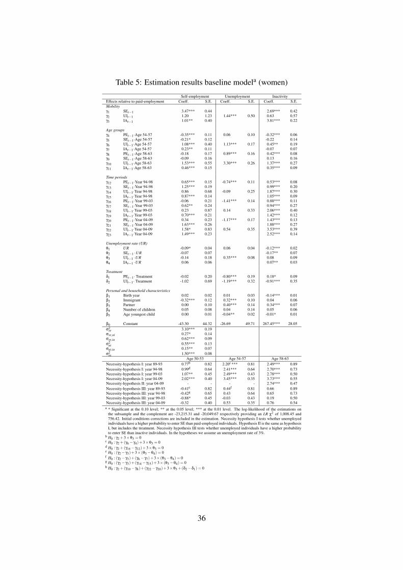
Table 5: Estimation results baseline modela (women)

Self-employment Unemployment InactivityEffects relative to paid-employment Coeff. S.E. Coeff. S.E. Coeff. S.E.Mobilityγ1 SEt−1 3.47*** 0.44 2.69*** 0.42γ2 UIt−1 1.20 1.23 1.44*** 0.50 0.63 0.57γ3 IAt−1 1.01** 0.40 3.81*** 0.22

Age groupsγ4 PEt−1 ·Age 54-57 -0.35*** 0.11 0.06 0.10 -0.32*** 0.06γ5 SEt−1 ·Age 54-57 -0.21* 0.12 -0.22 0.14γ6 UIt−1 ·Age 54-57 1.08*** 0.40 1.13*** 0.17 0.45** 0.19γ7 IAt−1 ·Age 54-57 0.23** 0.11 -0.07 0.07γ8 PEt−1 ·Age 58-63 -0.18 0.17 0.89*** 0.16 0.42*** 0.08γ9 SEt−1 ·Age 58-63 -0.09 0.16 0.13 0.16γ10 UIt−1 ·Age 58-63 1.53*** 0.55 3.30*** 0.26 1.37*** 0.27γ11 IAt−1 ·Age 58-63 0.46*** 0.15 0.35*** 0.09

Time periodsγ12 PEt−1 ·Year 94-98 0.65*** 0.15 -0.74*** 0.11 0.53*** 0.08γ13 SEt−1 ·Year 94-98 1.25*** 0.19 0.99*** 0.20γ14 UIt−1 ·Year 94-98 0.86 0.68 -0.09 0.25 1.87*** 0.30γ15 IAt−1 ·Year 94-98 0.87*** 0.14 1.05*** 0.09γ16 PEt−1 ·Year 99-03 -0.06 0.21 -1.41*** 0.14 0.88*** 0.11γ17 SEt−1 ·Year 99-03 0.62** 0.24 0.94*** 0.27γ18 UIt−1 ·Year 99-03 0.23 0.87 0.14 0.33 2.06*** 0.40γ19 IAt−1 ·Year 99-03 0.70*** 0.21 1.42*** 0.12γ20 PEt−1 ·Year 04-09 0.34 0.23 -1.17*** 0.17 1.43*** 0.13γ21 SEt−1 ·Year 04-09 1.63*** 0.26 1.88*** 0.27γ22 UIt−1 ·Year 04-09 1.58* 0.83 0.54 0.35 3.53*** 0.39γ23 IAt−1 ·Year 04-09 1.49*** 0.23 2.52*** 0.14

Unemployment rate (UR)θ1 UR -0.09* 0.04 0.06 0.04 -0.12*** 0.02θ2 SEt−1 ·UR -0.07 0.07 -0.17** 0.07θ3 UIt−1 ·UR -0.14 0.18 0.35*** 0.08 0.08 0.09θ4 IAt−1 ·UR 0.06 0.06 0.07** 0.03

Treatmentδ1 PEt−1 · Treatment -0.02 0.20 -0.80*** 0.19 0.18* 0.09δ2 UIt−1 · Treatment -1.02 0.69 -1.19*** 0.32 -0.91*** 0.35

Personal and household characteristicsβ1 Birth year 0.02 0.02 0.01 0.03 -0.14*** 0.01β2 Immigrant -0.32*** 0.12 0.32*** 0.10 0.04 0.06β3 Partner 0.00 0.10 0.40*** 0.14 0.34*** 0.07β4 Number of children 0.05 0.08 0.04 0.14 0.05 0.06β5 Age youngest child 0.00 0.01 -0.04** 0.02 -0.01* 0.01

β0 Constant -43.30 44.32 -26.69 49.71 267.45*** 28.05σ2

se 3.10*** 0.19σse,ui 0.27* 0.14σse,ia 0.62*** 0.09σ2

ui 0.55*** 0.13σui,ia 0.15** 0.07σ2

ia 1.50*** 0.08Age 50-53 Age 54-57 Age 58-63

Necessity-hypothesis I: year 89-93 0.77b 0.82 2.20c *** 0.81 2.49*** 0.89Necessity-hypothesis I: year 94-98 0.99d 0.64 2.41*** 0.64 2.70*** 0.73Necessity-hypothesis I: year 99-03 1.07** 0.45 2.49*** 0.43 2.78*** 0.50Necessity-hypothesis I: year 04-09 2.02*** 0.40 3.45*** 0.35 3.73*** 0.55Necessity-hypothesis II: year 04-09 - - - - 2.74*** 0.47Necessity-hypothesis III: year 89-93 -0.41e 0.82 0.44f 0.81 0.66 0.89Necessity-hypothesis III: year 94-98 -0.42g 0.65 0.43 0.64 0.65 0.73Necessity-hypothesis III: year 99-03 -0.88* 0.45 -0.03 0.43 0.19 0.50Necessity-hypothesis III: year 04-09 -0.32 0.40 0.53 0.35 0.76 0.54a * Significant at the 0.10 level; ** at the 0.05 level; *** at the 0.01 level. The log-likelihood of the estimations on

the subsample and the complement are -23,215.31 and -20,049.67 respectively providing an LR χ2 of 1,008.45 and756.42. Initial conditions corrections are included in the estimation. Necessity hypothesis I tests whether unemployedindividuals have a higher probability to enter SE than paid-employed individuals. Hypothesis II is the same as hypothesisI, but includes the treatment. Necessity hypothesis III tests whether unemployed individuals have a higher probabilityto enter SE than inactive individuals. In the hypotheses we assume an unemployment rate of 3%.

b H0 : γ2 +3×θ3 = 0c H0 : γ2 +(γ6− γ4)+3×θ3 = 0d H0 : γ2 +(γ14− γ12)+3×θ3 = 0e H0 : (γ2− γ3)+3× (θ3−θ4) = 0f H0 : (γ2− γ3)+(γ6− γ7)+3× (θ3−θ4) = 0g H0 : (γ2− γ3)+(γ14− γ15)+3× (θ3−θ4) = 0h H0 : γ2 +(γ10− γ8)+(γ22− γ20)+3×θ3 +(δ2−δ1) = 0

36

Table 6: Main income source and income level for those moving from inactivity to self-employment

Age 50-53 Age 54-57 Age 58-63%a Median incomeb % Median income % Median income

Men SEt Allt SEt Allt SEt AlltDisabilityt−1 18 18,645 22,006 27 19,616 22,452 26 17,863 23,082Early retirementt−1 7 17,788 30,424 8 26,620 35,015 16 29,240 35,453Social assistancet−1 17 6,423 13,670 5 3,199 13,462 5 8,1401 13,016Wealtht−1 32 47,982 38,164 39 54,470 40,581 43 44,307 27,687Income spouset−1 26 0 0 21 0 0 11 0 0WomenDisabilityt−1 3 14,108 13,776 6 13,029 13,723 6 8,743 13,735Early retirementt−1 5 14,085 21,426 3 11,846 21,340 16 10,144 19,672Social assistancet−1 5 16,279 15,076 5 18,587 15,002 2 11,735 14,897Wealtht−1 8 37,246 17,020 10 7,476 17,363 10 11,516 20,197Income spouset−1 79 0 0 76 0 0 66 0 0

a % refers to the percentage of inactive persons in t−1 who enter self-employment from a certain category.b The table shows median total income in period t− 1 for those individuals moving from a certain inactivity category to self-employment and for all individuals in that

inactivity category in t−1.

37

Table 7: Estimation results extended modelsa

Self-employment Unemployment InactivityEffects relative to paid-employment Coeff. S.E. Coeff. S.E. Coeff. S.E.Panel A. Financial variablesMenb

β6 Homeownert=0 0.23*** 0.07 -0.30*** 0.06 -0.08** 0.03β7 Mortgaget=0/106 0.21 0.21 -0.03 0.27 -0.35** 0.18β8 Financial wealtht=0/105 0.70*** 0.25 -0.40 0.66 -0.02 0.16β9 Net housing wealtht=0/105 -0.14 0.48 0.09 0.84 0.38 0.36β10 Risky assetst=0/103 0.43 0.47 0.06 0.37 -0.39* 0.20

δ1 PEt−1· Treatment 0.13 0.21 -0.53*** 0.14 0.08 0.08δ2 UIt−1·Treatment -0.52 0.59 -0.76*** 0.26 -0.12 0.28

Womenc

β6 Homeownert=0 0.42*** 0.07 -0.29** 0.07 0.00 0.05β7 Mortgaget=0/106 0.18 0.30 -0.07 0.29 -0.56** 0.23β8 Financial wealtht=0/105 0.26 0.25 -0.30 0.72 -0.01 0.20β9 Net housing wealtht=0/104 0.08 0.08 -0.03 0.10 0.03 0.06β10 Risky assetst=0/102 0.18 0.28 0.14 0.28 0.15 0.19

δ1 PEt−1· Treatment 0.05 0.21 -0.86*** 0.20 0.16* 0.10δ2 UIt−1·Treatment -1.08 0.70 -1.27*** 0.33 -1.03*** 0.37Panel B. HealthMend

β6 Bad healtht=0 -0.42*** 0.09 0.71*** 0.07 0.75*** 0.04

δ1 PEt−1· Treatment 0.12 0.20 -0.50*** 0.14 0.10 0.08δ2 UIt−1·Treatment -0.62 0.57 -0.65*** 0.25 -0.02 0.28

Womene

β6 Bad healtht=0 -0.54*** 0.12 1.22*** 0.09 0.70*** 0.06

δ1 PEt−1· Treatment -0.02 0.20 -0.88*** 0.19 0.17* 0.09δ2 UIt−1·Treatment -1.05 0.69 -1.01*** 0.32 -0.78** 0.35

a * Significant at the 0.10 level; ** at the 0.05 level; *** at the 0.01 level. All regressions include the variables from the baseline regression.b Financial variables are jointly significant with χ2(15) = 95.87 and p− value = 0.000. The log-likelihood of the estimations on the subsample and the complement are

-24,793.58 and -22,030.97 respectively providing an LR χ2 of 980.40 and 901.99.c Financial variables are jointly significant with χ2(15) = 99.08 and p− value = 0.000. The log-likelihood of the estimations on the subsample and the complement are

-19,339.93 and -20,029.29 respectively providing an LR χ2 of 889.92 and 767.43.d The log-likelihood of the estimations on the subsample and the complement are -27,076.24 and -21,939.01 respectively providing an LR χ2 of 1,056.45 and 866.57.e The log-likelihood of the estimations on the subsample and the complement are -23,100.08 and -19,991.02 respectively providing an LR χ2 of 993.69 and 743.59.

38

Table 8: Robustness checksa

Self-employment Unemployment InactivityEffects relative to paid-employment Coeff. S.E. Coeff. S.E. Coeff. S.E.Panel A. Placebo testsMen: placebo age 56-57δ1 PEt−1· Treatment 0.20 0.27 0.29 0.19 -0.08 0.13δ2 UIt−1·Treatment -0.39 0.96 0.28 0.33 0.17 0.38

Women: placebo age 56-57δ1 PEt−1· Treatment -0.06 0.16 0.01 0.14 0.07 0.07δ2 UIt−1·Treatment -0.12 0.52 -0.04 0.25 0.13 0.29

Men: placebo year 2000-2003δ1 PEt−1· Treatment -0.23 0.31 0.18 0.21 0.21** 0.09δ2 UIt−1·Treatment 0.36 1.40 0.32 0.44 0.20 0.47

Women: placebo year 2000-2003δ1 PEt−1· Treatment -0.11 0.24 0.34 0.21 0.18** 0.09δ2 UIt−1·Treatment -12.91 556.15 0.34 0.34 -0.04 0.40Panel B. Smaller time windowMenδ1 PEt−1· Treatment -0.02 0.32 0.05 0.22 0.10 0.11δ2 UIt−1· Treatment -0.44 1.12 -0.70* 0.41 -0.43 0.43

Womenδ1 PEt−1· Treatment 0.06 0.24 0.06 0.21 0.36*** 0.10δ2 UIt−1·Treatment -0.92 0.75 -0.79** 0.35 -0.47 0.39Panel C. SingleMenδ1 PEt−1· Treatment 0.07 0.21 -0.51*** 0.14 0.09 0.08ϑ1 PEt−1· Treatment · Single 0.16 0.35 0.06 -0.09 0.09 0.11δ2 UIt−1· Treatment -0.42 0.61 -0.67*** 0.27 -0.03 0.30ϑ2 UIt−1· Treatment · Single -0.80 0.93 -0.52 0.35 -0.52 0.40

Womenδ1 PEt−1· Treatment 0.11 0.21 -0.87*** 0.21 0.21** 0.09ϑ1 PEt−1· Treatment · Single -0.81** 0.37 0.27 0.26 -0.13 0.11δ2 UIt−1·Treatment -1.37* 0.71 -1.43*** 0.34 -1.05*** 0.39ϑ2 UIt−1·Treatment · Single -11.47 310.90 0.63 0.49 0.69 0.56

a * Significant at the 0.10 level; ** at the 0.05 level; *** at the 0.01 level. Results of the different robustness checks are estimated separately. All regressions include the variablesfrom the baseline regression including the initial conditions correction and correlated random effects parameters. Single is a binary variable with a value of one for singleindividuals and zero otherwise.

39

Table 9: Simulation resultsa,b

Men WomenYear t

Year t−1 PE SE UI IA PE SE UI IAPE 73.13 0.19 2.77 23.90 48.86 1.09 1.71 48.34

(1.41) (0.03) (0.34) (1.44) (2.37) (0.19) (0.32) (2.43)SE 12.67 4.58 0.52 82.23 7.94 17.34 0.36 74.36

(1.34) (0.57) (0.07) (1.57) (1.01) (1.84) (0.06) (2.14)UI 2.14 0.29 81.95 15.61 1.19 1.12 36.10 61.59

(0.75) (0.12) (1.97) (1.88) (0.32) (0.59) (5.55) (5.61)IA 1.75 0.22 0.07 97.95 0.63 0.28 0.03 99.06

(0.12) (0.03) (0.00) (0.13) (0.05) (0.03) (0.00) (0.06)Treatment effectsPE -0.61 0.01 -1.12 1.72 -3.86 -0.11 -1.01 4.97

(2.01) (0.04) (0.35) (1.42) (2.18) (0.21) (0.29) (2.24)UI 2.00 0.00 -11.85 9.84 1.96 -0.08 -6.70 4.81

(0.75) (0.16) (2.83) (2.73) (0.71) (0.71) (5.11) (5.34)a This table presents a simulated transition matrix for a reference individual, which is a native male or female with a partner, without children in the

same household, and of age 60 in the year 2006.b Standard errors in parentheses (1500 bootstrap replications).

40