The NASA Subsonic Jet Particle Image Velocimetry (PIV) Dataset · 2013-04-10 ·...

James Bridges and Mark P. WernetGlenn Research Center, Cleveland, Ohio

The NASA Subsonic Jet Particle Image Velocimetry (PIV) Dataset

NASA/TM—2011-216807

November 2011

https://ntrs.nasa.gov/search.jsp?R=20110023688 2020-06-30T05:11:56+00:00Z

NASA STI Program . . . in Profile

Since its founding, NASA has been dedicated to the advancement of aeronautics and space science. The NASA Scientific and Technical Information (STI) program plays a key part in helping NASA maintain this important role.

The NASA STI Program operates under the auspices of the Agency Chief Information Officer. It collects, organizes, provides for archiving, and disseminates NASA’s STI. The NASA STI program provides access to the NASA Aeronautics and Space Database and its public interface, the NASA Technical Reports Server, thus providing one of the largest collections of aeronautical and space science STI in the world. Results are published in both non-NASA channels and by NASA in the NASA STI Report Series, which includes the following report types: • TECHNICAL PUBLICATION. Reports of

completed research or a major significant phase of research that present the results of NASA programs and include extensive data or theoretical analysis. Includes compilations of significant scientific and technical data and information deemed to be of continuing reference value. NASA counterpart of peer-reviewed formal professional papers but has less stringent limitations on manuscript length and extent of graphic presentations.

• TECHNICAL MEMORANDUM. Scientific

and technical findings that are preliminary or of specialized interest, e.g., quick release reports, working papers, and bibliographies that contain minimal annotation. Does not contain extensive analysis.

• CONTRACTOR REPORT. Scientific and

technical findings by NASA-sponsored contractors and grantees.

• CONFERENCE PUBLICATION. Collected papers from scientific and technical conferences, symposia, seminars, or other meetings sponsored or cosponsored by NASA.

• SPECIAL PUBLICATION. Scientific,

technical, or historical information from NASA programs, projects, and missions, often concerned with subjects having substantial public interest.

• TECHNICAL TRANSLATION. English-

language translations of foreign scientific and technical material pertinent to NASA’s mission.

Specialized services also include creating custom thesauri, building customized databases, organizing and publishing research results.

For more information about the NASA STI program, see the following:

• Access the NASA STI program home page at http://www.sti.nasa.gov

• E-mail your question via the Internet to help@

sti.nasa.gov • Fax your question to the NASA STI Help Desk

at 443–757–5803 • Telephone the NASA STI Help Desk at 443–757–5802 • Write to:

NASA Center for AeroSpace Information (CASI) 7115 Standard Drive Hanover, MD 21076–1320

James Bridges and Mark P. WernetGlenn Research Center, Cleveland, Ohio


NASA/TM—2011-216807

November 2011

National Aeronautics andSpace Administration

Glenn Research Center Cleveland, Ohio 44135

Acknowledgments

The authors gratefully acknowledge the hard work and long hours put in by the technicians and engineers at the AeroAcoustics Propulsion Laboratory and by the research technicians who helped in setup and operation of the PIV systems. The data contained within this report were acquired primarily during the Quiet Aircraft Technology Program at NASA, and support of management for this fundamental effort is commended. Finally, the review of this manuscript by Dennis Yoder and Abbas Khavaran was very helpful in assuring accuracy and accessibility to the reader.

Available from

NASA Center for Aerospace Information7115 Standard DriveHanover, MD 21076–1320

National Technical Information Service5301 Shawnee Road

Alexandria, VA 22312

Available electronically at http://www.sti.nasa.gov

Trade names and trademarks are used in this report for identification only. Their usage does not constitute an official endorsement, either expressed or implied, by the National Aeronautics and

Space Administration.

This work was sponsored by the Fundamental Aeronautics Program at the NASA Glenn Research Center.

Level of Review: This material has been technically reviewed by technical management.

NASA/TM—2011-216807 1


James Bridges and Mark P. Wernet National Aeronautics and Space Administration

Glenn Research Center Cleveland, Ohio 44135

Abstract

Many tasks in fluids engineering require knowledge of the turbulence in jets. There is a strong, although fragmented, literature base for low order statistics, such as jet spread and other mean-velocity field characteristics. Some sources, particularly for low speed cold jets, also provide turbulence intensities that are required for validating Reynolds-averaged Navier-Stokes (RANS) Computational Fluid Dynamics (CFD) codes. There are far fewer sources for jet spectra and for space-time correlations of turbulent velocity required for aeroacoustics applications, although there have been many singular publications with various unique statistics, such as Proper Orthogonal Decomposition, designed to uncover an underlying low-order dynamical description of turbulent jet flow. As the complexity of the statistic increases, the number of flows for which the data has been categorized and assembled decreases, making it difficult to systematically validate prediction codes that require high-level statistics over a broad range of jet flow conditions.

For several years, researchers at NASA have worked on developing and validating jet noise prediction codes. One such class of codes, loosely called CFD-based or statistical methods, uses RANS CFD to predict jet mean and turbulent intensities in velocity and temperature. These flow quantities serve as the input to the acoustic source models and flow-sound interaction calculations that yield predictions of far-field jet noise. To develop this capability, a catalog of turbulent jet flows has been created with statistics ranging from mean velocity to space-time correlations of Reynolds stresses. The present document aims to document this catalog and to assess the accuracies of the data, e.g., establish uncertainties for the data.

This paper covers the following five tasks: • Document acquisition and processing procedures used to create the particle image velocimetry

(PIV) datasets. • Compare PIV data with hotwire and laser Doppler velocimetry (LDV) data published in the open

literature. • Compare different datasets acquired at roughly the same flow conditions to establish

uncertainties. • Create a ‘consensus’ dataset for a range of hot jet flows, including uncertainty bands. • Analyze this consensus dataset for self-consistency and compare jet characteristics to those of the

open literature. One final objective fulfilled by this work was the demonstration of a universal scaling for the jet flow

fields, at least within the region of interest to aeroacoustics. The potential core length and the spread rate of the half-velocity radius were used to collapse of the mean and turbulent velocity fields over the first 20 jet diameters in a highly satisfying manner.

Nomenclature Dj diameter of jet exit Ma acoustic Mach number, = Uj/c∞ Mj jet Mach number, = Uj/cj

NASA/TM—2011-216807 2

T∞ temperature of freestream/ambient Tj jet static temperature at jet exit, assuming fully expanded flow U mean value of velocity U∞ velocity of freestream/ambient Uj jet velocity at jet exit, assuming fully expanded flow Xc potential core length defined by experimental collapse of u′/U∞ on jet centerline Xw potential core length defined by Witze (Ref. 16) Yc jet spread factor, = 2ψx+Dj c∞ speed of sound in freestream/ambient cj speed of sound in jet fluid at jet exit, assuming fully expanded flow r radial coordinate r0.5 location of half-velocity point in radial velocity profile u′ root mean square value of velocity x streamwise coordinate y transverse coordinate δω shear layer thickness, Uj/|dU/dr|max η shear layer coordinate, = (r – r0.5)/δω, η∗ shear layer growth rate coordinate = (r – r0.5)/x θ boundary layer momentum thickness at nozzle lip ν kinematic viscosity ψ jet spread rate, = (r0.5 – Dj/2)/x

1.0 Introduction Several articles in the open literature document previous efforts to measure turbulent jets. Most were

acquired in cold, low speed jets, often using hotwire anemometry, although some results from laser Doppler velocimetry (LDV) were found and parts of these include measurements of hot jets. The data sources used are References 1 to 15. Many of these were digitized and converted into a common format for comparison to the current PIV data.

The earliest source commonly cited for turbulence measurements in jets is Laurence in 1954 (Ref. 1). This detailed NACA report is detailed and deep, containing jet data of mean, variance, spectra, space and time correlations and length and timescale integrals for Mach numbers in a range from 0.2 through 0.7. The data was acquired using the then-new technology of constant temperature anemometry and used variable length loops between tape heads to compute time-delay correlations. Unfortunately, when compared against the majority of data, it appears that the turbulence intensities were understated, perhaps as a result of uncorrected high frequency rolloff.

The early 1960s were an active time for jet noise-related turbulence measurements using hotwire anemometry, with Journal of Fluid Mechanics publishing extensive jet turbulence measurements by Davies, Fisher and Barrett in 1963 (Ref. 2),Fisher and Davies (Ref. 3), and Bradshaw, Ferriss and Johnson (Ref. 4) in 1964. These papers contained an extensive host of data, from mean shear statistics to convective velocity and space-time correlations. Although the format of the Journal precluded extensive database reproduction and the depth also foreshortened how much data for any given statistic could be presented, these papers commonly presented radial and axial profiles of axial turbulence. Radial profiles were often presented for the shear layer, typically at x/Dj = 2 or 4 which is well within the jet potential core, and normalized by η* = (r – r0.5)/x, where r0.5 is the radial location where the jet mean velocity is half the profile peak value. Others have since chosen to normalize the radial profiles by local maximum shear gradient, or η = (r – r0.5)/δω, where δω is Uj/|dU/dr|max. The ratio between η and η* is x/δω which is a measure of the shear layer spread and is roughly constant for two-dimensional shear layers. Davies et al., like Laurence, documented the impact of Mach number on basic turbulence levels. Given that the Mach numbers were below 0.5 and that the nozzles were 1 and 2 in. in diameter, it is possible that these

NASA/TM—2011-216807 3

measurements were subject to Reynolds number effects as well as the initial turbulence levels rather than compressibility effects. Bradshaw et al., working with cross-wires, documented all three components of turbulence. All three papers present extensive length scale estimates from correlation measurements.

In the early 1970s attention turned toward obtaining insight into what has become known as coherent structures in the jet flow. Papers such as Ko and Davies (Ref. 5) explored the interesting inhomogeneities of the jet spectra, giving rise to interest in the structure of the jet as a way to simplify the description of the turbulence as it relates to jet noise. Use of external sources of perturbation to dominate the natural perturbations in the jet spawned several important studies. Crow and Champagne (Ref. 6) in 1971 documented the impact of jet excitation on standard turbulence statistics, and introduced measurements that are useful in jet instability studies. In 1978 Raman, Zaman and Rice (Ref. 7) produced useful basic turbulence statistics of jets as they explored the role of initial turbulence on the ability to excite a jet. Later in the 1970s not only were experimentalists turning their attention to new statistical descriptions to educe these large-scale structures, they were also using a new laser-based, non-invasive measurement technique: Laser Doppler Velocimetry (LDV). Of note here for the purpose of basic jet turbulence statistics are the papers of Lau and collaborators (Refs. 8, 9, and 10). Lau, Morris and Fisher (Ref. 8) compared the hotwire and LDV measurements and showed that at that time LDV measurements of turbulence were not quite comparable (Fig. 4 in the paper). However, this was soon rectified in subsequent papers and the advantage of the LDV at high speed and elevated temperature jets, allowed Lau (Ref. 9) to document the impact of high speed on basic turbulence statistics, and Lau (Ref. 10) extended the effort to hot jets. In this latter work Lau focuses mostly on gross features of spread rates and nondimensionalizing the jet potential core, but it is a data-dense paper even so. LDV also allowed an extensive dataset to be collected for unexcited and excited unheated and heated jets by Lepicovsky and collaborators, herein referenced through the NASA contractor report by Ahuja (Ref. 11) in 1982.

With such extensive datasets available, few authors have documented the basic measures of jet turbulence in recent papers. One exception is Zaman (Ref. 12), that documented the impact of lobed mixers on centerline statistics of the jet. Another exception is Kerherve et al. (Ref. 13) that measured a supersonic jet in a forward flight environment. That work contains plots of radial turbulence intensity profiles at various axial stations in a shock-containing jet. It should be noted that they normalized the turbulence by the jet/ambient velocity difference Uj – U∞ and found a peak value of 17 percent at all stations. Most recently (2009), Morris and Zaman (Ref. 14) have repeated measurements of turbulence in low speed jets with the objective of obtaining an extensive and consistent set of high order statistics, and in the process have documented their radial and centerline turbulence profiles.

Of course, while the new LDV technology brought about fresh measurements, so did the advent of PIV. Besides the current authors’ papers, a notable work by Pokora (Ref. 15) as carefully documented PIV measurements in a water jet, highlighting the differences found between two-and three-component PIV systems. Just as hotwire anemometry allowed measurement of unsteady velocity and LDV allowed measurement of high speed and hot jets, so did PIV bring about a multi-order of magnitude increase in information density. Instead of having roughly 10 points to define a profile now there are hundreds. Where once datasets could be written by hand in a single notebook, now it requires gigabytes of storage to hold the dataset of a single jet flow. And it has greatly enhanced the types of analysis that is possible. This has raised challenges in presenting the PIV datasets and making them available to interested researchers.

So just how do data from different sources compare? To find out, the graphs from the referenced papers were digitized and the data read electronically and a common dimensionless variable u′/Uj was plotted versus axial distance or radial coordinate. For axial distances we use both the jet diameter Dj and the jet potential core length Xc as normalization factors. The potential core length was computed using the formula of Witze (Ref. 16). The radial coordinate r, was normalized as local shear layer coordinate η = (r – r0.5)/δω, i.e., the radial coordinate has been normalized by the local mean velocity gradient as best as could be ascertained from the papers’ data.

NASA/TM—2011-216807 4

Figure 1.—Axial profiles of axial turbulence on jet centerline as reported in the literature. Axial coordinate is

normalized by jet diameter Dj (left) and by potential core length XW (right). Turbulence is most commonly shown along the jet centerline, although this does not correspond to

the peak turbulence level in the jet, another quantity of interest. In Figure 1, data from the literature covering a range of Mach numbers from 0.11 to 0.8 are plotted against axial distance normalized by jet diameter. This results in a rather large scatter among the data. In the figure, open symbols are hotwire data while the few closed symbols are LDV measurements. As the data are colored by Mach number, it is easy to see the effect of Mach number on where the peak occurs. When the axial coordinate is normalized by potential core length Xc a satisfying collapse of the data results. A few of the outliers are surprising: The data of Bradshaw et al. and of Laurence are startlingly off given their citation count. Ignoring these two datasets, the peak axial turbulent velocity on the centerline is found to be 0.13 with a spread of 0.005 located roughly 1.5 potential core lengths downstream of the nozzle exit.

Because x/Dj = 4 is a commonly used location for radial profiles, and because this location is not sensitive to variations in potential core length, data at this location were compiled for comparison of radial profiles for low subsonic cold jets, presented in Figure 2. Color is again used to separate the speeds, ranging from very small Mach for the water jet data of Pokora to M = 0.5. Filled symbols denote LDV measurements and an open X is the PIV data of Pokora, which falls outside the range of the other data. Ignoring this dataset, there is good agreement on the width of the shear layer, but a variation in peak amplitude of roughly u′/Uj = 0.02 out of 0.16, or roughly 12 percent uncertainty. There is no improvement in this variation by concentrating on datasets containing only hotwire data sources. There is a bit of a systematic variation in peak amplitude with Mach number in the hotwire datasets. The LDV datasets, acquired at Mach numbers comparable to the highest of the hotwire measurements does not follow this trend. At this point it is possible that there is no valid trend with Mach number or that the LDV data is biased to higher turbulence amplitudes.

Radial profiles for cold jets of M greater than 0.5 are plotted in Figure 3. Data is presented from hot wire, LDV, and PIV velocimetry systems. Here the spread is roughly 50 percent, with peak turbulence intensity ranging from 0.10 to 0.17! There is a clear bias with anemometry type, with the two LDV datasets being significantly above all the other data. There is no trend with Mach number or age of the data. At this stage it seems prudent to remove the excessively low hotwire data of Narayanan and perhaps weigh the LDV data a little less strongly than the preponderance of hotwire data that are in relative agreement. Doing so gives an estimate of peak axial turbulent velocity of 0.14 very near the half-velocity point, with a spread of roughly –0.01/0.02.

Unfortunately, no more than one dataset of a hot subsonic jet could be located for either a centerline profile or a radial profile.

NASA/TM—2011-216807 5

Figure 2.—Radial profiles of axial turbulence at x/Dj ~ 4

for low subsonic, cold jets, as reported in the literature.


for high subsonic, cold jets, as reported in the literature.

2.0 Descriptions of NASA Facility, PIV Operations, and Test Programs 2.1 Facility Description

All original data presented in this document were acquired in the Small Hot Jet Acoustic Rig (SHJAR) at NASA Glenn Research Center. Other extensive datasets have also been acquired on a larger, higher fidelity jet rig, but for more complicated nozzle configurations that are harder to verify against independent sources. It is expected that, since the PIV and seeding systems are similar between the two rigs, uncertainties established by the present exercise can be carried over to the datasets acquired in the larger rig.

NASA/TM—2011-216807 6

The Small Hot Jet Acoustic Rig (SHJAR, pronounced with a silent ‘J’), shown in Figure 4, is located in the Aeroacoustic Propulsion Laboratory (AAPL) at the NASA Glenn Research Center in Cleveland, Ohio. The SHJAR was developed to test jet noise reduction concepts at a low technology readiness level (TRL 1 to 3) and at minimum expense. The AAPL, which houses the SHJAR, is a geodesic dome (60-ft radius) lined with sound absorbing wedges which reduce sound reflection at all frequencies above 200 Hz. The jet exhaust is directed outside through a large door that permits unrestricted flow seeding operation without introducing noise interference concerns related to particulate collection systems.

As a jet noise testing rig, the SHJAR was designed to minimize rig noise sources, incorporating the recommendations of Viswanathan (Ref. 17) and Ahuja (Ref. 18) to achieve this goal. The rig is a single flow jet rig that used 150-psi air supplied by several remotely located compressors. The maximum mass flow rate was 6 lbm/s and the maximum temperature air was 1300 °F. A hydrogen-fueled combustor permits a large range of temperature flows to be tested. The air passes through a baffled muffler and settling chamber before it reaches the nozzle. Two valves, a large main valve and a small vernier valve located upstream of the combustor and muffler, control the rate of airflow, providing fine control over the entire range of operating conditions. Flow conditions are measured in the 14 in. (356 mm) diameter plenum chamber located within the supporting frame. An ASME contraction connects the plenum chamber to a 6 in. (150 mm) diameter nozzle feedpipe that is 25 in. (635 mm) long. An extensive study of the acoustic properties of the SHJAR rig and its validation are given in Brown and Bridges (Ref. 19).

Figure 4.—Small Hot Jet Acoustic Rig (SHJAR).

NASA/TM—2011-216807 7

2.2 Test Nomenclature

This report covers testing done from October 2001 through August 2007. Roughly once a year a test campaign was mounted which required PIV testing in the SHJAR. With each entry the implementation of PIV was changed in some way, to either address lessons learned from previous testing or to add new capability, such as a third velocity component, faster data acquisition rate or kHz time resolution. Whenever possible, data for a matrix of points was acquired, aiming to duplicate, or improve upon, previous measurements. This repeat of conditions with varying PIV configurations has allowed a certain insight into data uncertainty that is very valuable for engineering practice.

The set of flow conditions that were chosen for repeat testing was a subset of the matrix created by Plumblee et al. (Ref. 20) (conventionally known as the Tanna matrix). This matrix is defined on constant acoustic Mach number Ma (jet velocity normalized by ambient speed of sound) and constant static temperature ratio Tj/T∞ (static temperature relative to ambient temperature). The matrix of flow conditions considered in the current report is given in Table 1. Table 2 lists the test entries, which were known by mnemonics that usually include the NASA fiscal year and some indication of the test content. For this report the test entries have been labeled T0 through T6 and will be referred to in describing datasets, experimental setups, etc. Under the heading ‘PIV Configuration’, the table notes whether the data plane is streamwise (X, Y, Z=0) or cross-stream (X=c, Y, Z), whether two or three components of velocity were acquired, and whether there was temporal measurements available, either as fixed time delays (T = τ) or for a continuous record in time (T). The table also lists the nozzles tested and some insight into the original purpose of the test.

TABLE 1—DEFINITION OF TEST CONDITIONS

Set point Ma Tj/T∞ NPR M 3 0.500 0.950 1.197 0.513 7 0.900 0.835 1.861 0.985

23 0.500 1.764 1.102 0.376 27 0.900 1.764 1.357 0.678 29 1.330 1.764 1.888 1.001 46 0.900 2.700 1.219 0.548 49 1.485 2.700 1.678 0.904

TABLE 2.—DESCRIPTION OF TEST ENTRIES

Test entry

Test name

Dates PIV configuration

Nozzles tested

Purpose

T0 SHJARCHK October 2001 X,Y,Z=0; U,V

ARN1, ARN2

Initial checkout of SHJAR

T1 SHJARBASE1 April 2002 X,Y,Z=0,T=τ; U,V

ARN2 Dual-PIV for space-time correlations

T2 SHJARCHEV04 November 2003 X=c,Y,Z; U,V,W

ARN2, SMC00x

Cross-stream, three-component

T3 SHJARBASE2 December 2003 X,Y,Z=0; U,V,W

ARN2, SMC00x

Streamwise, three-component

T4 SHJARBASE05 January 2004 X,Y,Z=0; U,V,W

SMC000, SMC01x

Streamwise, three-component, supersonic nozzles

T5 TRPIV06 May 2006 X,Y,Z=0,T; U,V

SMC000 Time-resolved PIV

T6 TRPIV07 June-August 2007 X,Y,Z=0,T; U,V

SMC000, SMC01x

Time-resolved PIV on supersonic nozzles

2.3 Nozzle Description

Some of the nozzles used in this report were from a family of convergent nozzles, called the Acoustic Reference Nozzles (ARN), designed to be simple to characterize with similar dimensions such as inlet diameter (6.0 in./15.24 mm), lip thickness (0.050 in./1.27 mm), outside face angle (30° to jet axis), and

NASA/TM—2011-216807 8

parallel flow section at the exit (0.25 in./6.4 mm). In some data reported here, acquired before 2003, the ARN1, a 1 in./25.4 mm diameter nozzle, and ARN2, a 2 in./50.1 mm diameter nozzle, were used. These are shown connected to the feedpipe in Figure 5 .

The ARN series of nozzles featured a relatively strong contraction that resulted in relaminarization of the boundary layer, especially at low Reynolds numbers, and potentially caused some Reynolds number dependence of the jet’s behavior. Since the point of nozzle testing is to simulate large-scale nozzles, e.g., high Reynolds number, with initially turbulent shear layers, it is desired to avoid relaminarization in the nozzle contraction.

To avoid relaminarization and to provide a baseline for a series of simple chevron nozzles, the Small Metal Chevron (SMC) nozzle system was developed. Originally conceived as a model system for parametric testing of chevron nozzles, its modular design has lent itself to a large number of nozzle concepts being mounted on it, including chevrons and convergent-divergent nozzles. The baseline axisymmetric convergent nozzle, SMC000, is shown in Figure 6. It has an exit diameter of 2 in./50.8 mm.

In 2004 and 2005, a series of measurements were made with hotwire anemometry to characterize the exit boundary layer/initial shear layer of the ARN and SMC nozzles by measuring velocity profiles at the nozzle exits at low Mach numbers. Classically, one expects that laminar boundary layers will have a shape which, when quantified by the ratio of momentum thickness and displacement thickness, will produce a value, called the shape factor, of roughly 2.5. Fully turbulent boundary layers have shape

Figure 5.—SHJAR nozzle system with Acoustic Research Nozzle 1

(ARN1) and 2 (ARN2) attached.

Figure 6.—SHJAR nozzle system with SMC000 nozzle attached.

NASA/TM—2011-216807 9

factors closer to 1.8. Another indicator of an initially turbulent shear layer is the turbulence intensity, u′/Uj, which ranges from immeasurably small for a truly laminar case, to as much as 10 percent for an intensely turbulent boundary layer.

Figure 7 contains three plots from these hot wire tests, one each with the shape factor, the peak turbulence intensity, and the momentum thickness as a function of Reynolds number, ReD = UjDj/ν. Two nozzles are shown, although different upstream treatment has been applied to these nozzles, as specified in the plot legends. The ARN2 and SMC000 nozzles were measured in both 2004 and 2005, but between the years (in April 2004, specifically; between test entries T3 and T4) a series of screens 12 to 14 in. upstream of the nozzle were removed. In both cases this slightly raised the shape factor (more laminar). It also strongly decreased the peak turbulence. This was not appreciated at the time since other factors, including acoustics, showed that the smc000 was not suffering from known laminar artifacts. For comparison, the ARN2 nozzle was tested with a significant trip placed in the contraction and the boundary layer parameters for this very turbulent initial condition are shown in the plots. This configuration was not tested using PIV. The impact of the screen removal on the flow can be determined by comparing to SMC000 data acquired in the T3 and T4 test programs. In Section 5.2 it will be concluded that no difference could be determined from looking at plots of mean velocity or turbulence intensity.

Figure 7.—Boundary layer statistics (shape factor, peak turbulence level, momentum thickness) for ARN2 and

SMC000 nozzles for low Reynolds numbers (0.1 < Ma < 0.5).

NASA/TM—2011-216807 10

2.4 Particle Image Velocimetry Systems Details of the various PIV installations are given in References 23, 24, 21, and 22. Below are some

common aspects of the installations, provided to give the reader some level of detail on this critical aspect of the dataset.

2.4.1 Two-Component Stereoscopic PIV System (T0, T1) Two-component PIV systems with the light sheet oriented parallel to the flow direction were used in

the T0 and T1 test entries. In the T0 entry the PIV system components were located on the traversing mechanism, colloquially known as Big Blue, shown in Figure 8. Nozzle flow surveys were obtained by traversing the PIV system along the jet axis using the large traverse system. A Continuum PIV-Surelite III, 400 mJ per pulse at 532 nm, dual head, Nd:YAG laser operating at 10 Hz produced the pulsed light sheets. For the T0 experimental configuration an interframe time of 1.2 μs was used. A laser light sheet approximately 0.2 mm thick was formed with one cylindrical and one spherical lens and directed along the jet axis. A Redlake ES 4.0 digital camera with a 2048×2048 pixel CCD array was used to record the PIV images. The PIV camera was configured for a 136 mm field. Particle displacements ranging from 0 to 17 pixels were measured, resulting in a full-scale error of 0.5 percent after subpixel particle image fitting. Four hundred image pairs or velocity maps were acquired for each axial location and were used in the statistical processing of the turbulence data. The full-scale errors given above were, therefore, reduced further through the averaging process. The PIV images were processed with PIVPROC (Ref. 27), a GRC-developed code. PIVPROC uses a correlation-based processing algorithm that allows for subregion image shifting and multi-pass correlation to improve the spatial resolution of the resultant velocity vector maps. The first pass of the correlation used a subregion size of 64×64 pixels with 50 percent overlap. The second pass used a 32×32 pixel subregion size, again with 50 percent overlap. The resulting spatial resolution of the velocity vector fields was 1.06 mm for the 136 mm fields of view.

Figure 8.—PIV setup for test entry T0. Left: Laser and beam-forming optics below, light sheet impinging upon bottom

of nozzle, black velvet covered optical background for cameras in upper left of image. Right: Light sheet impinging upon nozzle, camera mounted 12 in. away, ‘tent’ around the SHJAR frame to guide ambient seeding from oil vapor smoke generator. Eggshell foam on the rig is for acoustic measurements—not PIV.

NASA/TM—2011-216807 11

In the T1 entry there were actually two complete (laser and camera) two-component PIV systems, identical to the ones used in T0, but phase locked together to allow variable time delay between the velocity field measurements. Details of this system and its results are found in Reference 23 and a sketch and photo of the layout is given in Figure 9. Each PIV system consisted of a Continuum Surelite III dual head Nd:YAG laser operating at 532 nm generating a 400 mJ/pulse light sheets aligned with the axis of the jet. Each laser/light sheet system was configured with its own Redlake ES 4.0 camera with 2000×2000 pixel resolution. Each camera viewed the light sheet at right angles, one on each side of the light sheet. A computer equipped with a frame digitizer was used to acquire image data to memory in 200 image-pair sequences, which were then saved to disk. Each camera viewed the same 170 mm square field of view, centered on the jet axis, from a distance of 1.4 m. The Redlake ES 4.0 cameras are frame-straddling cameras and consequently the second exposure in an image frame pair has a long integration period (200 ms). Because the AAPL is open to the outdoors and could not be run in total darkness, optical backgrounds for the cameras had to be provided to minimize the ambient light contaminating the long second exposure images. The cameras each peered through aluminum plates covered in black velvet, providing a dark uniform background for each other. These are not shown in Figure 9 for clarity.

Figure 9.—Dual PIV setup for test entry T1. Left: Drawing of side view showing positioning of two PIV systems, each

with its own laser power supplies, laser head, camera, and control computer. Center: photograph of dual PIV system in action. Fixed system is on the left and translated system is on the right. Right: diagram of polarization scheme deployed to allow overlapping fields of view with independent PIV systems.

C P U

P S 2P S 1P S 1 P S 2

21

o n

e n s

λ/2

“p”-Polarizer

“s”-Polarizer

PIV Camera # 1

PIV Camera # 2

Laser # 2

Laser # 1

NASA/TM—2011-216807 12

Both PIV systems were mounted on a large axial traverse that carried all power supplies, laser heads, cameras, and acquisition computers, as shown in Figure 9. This traverse had a range of roughly 2.5 m with an accuracy of 1 mm. One of the PIV systems was further mounted on a secondary axial traverse atop the primary traverse, giving it a displacement relative to the primary, or fixed, PIV system. The laser head and light sheet forming optics were mounted on one high-precision positioner while the associated camera was mounted on a synchronized positioner. The secondary traverse had a range of 1 m with an accuracy of 0.01 mm. Alignment of the two PIV systems was accomplished by registering both camera images on a two-sided optical target in the plane of the light sheet and by registering of the light sheets on a fixed target using light sensitive paper, paying special attention to the lower intensity edges of the light sheet burn images on the paper. The light sheets had to remain aligned for the full length of the secondary PIV system range of travel.

Key to the success of the effort was the use of cross-polarization of the laser beams and polarizers on the PIV cameras. The primary PIV system was configured to use ‘p’-polarized light and its camera was equipped with a polarizer to only pass ‘p’ polarized light, see Figure 7. The second, translating PIV system was configured to use ‘s’-polarized light while its camera only sensed ‘s’-polarized light. Without this polarization isolation, light from the second PIV system laser became a ‘noise’ to the first system’s second image, raising the signal to noise ratio of the image cross-correlation to an unacceptable level. Polarization isolation reduced the image intensity of the second PIV system on the primary PIV system to a level which allowed successful cross-correlation for both systems.

Velocity maps were computed from the image pairs using conventional multipass PIV algorithms with error detection based upon image correlation signal to noise ratio (NASA PIVPROC software). All datasets used had a data quality metric of 0.9 or better, where data quality is defined as the number of accepted velocity vectors at a location relative to the total number of image pairs acquired. Final velocity maps had a spatial resolution of 0.02 Dj. A minimal number of velocity maps (200) were acquired at each space-time separation to obtain rough estimates of the correlations. Based upon convergence of the statistics, the error in the final correlation data was estimated at ±5 percent.

2.4.2 Three-Component PIV With the T2, T3, and T4 entries, stereoscopic particle image velocimetry was implemented to

measure all three components of velocity. Full details are given in Reference 24. When measuring jets with three-dimensional nozzles, such as lobed or chevron nozzles, it is more efficient to obtain data in a plane normal to the flow rather than to piece together multiple streamwise planes. This also allows measurement of axial vorticity, a valuable statistic in understanding the role of enhanced mixing devices on jet noise.

In stereo imaging of a flow field, two viewing modes are possible. In the first configuration, shown in Figure 10, both cameras are located on the same side of the laser light sheet, which is a suitable arrangement for cross-plane jet flow measurements. In the second configuration, shown in Figure 11, the cameras are located on opposite sides of the light sheet. This arrangement is suitable for streamwise (axial-plane) measurements. In the cross-flow configuration used in T2, there is no alternative set of camera orientations to eliminate the nozzle from the camera fields-of-view for measurement planes close to the nozzle. However, for the axial-flow configuration used in T3 and T4, two separate camera orientations are possible.

Rather than positioning the cameras in the horizontal xz-plane, which keeps the nozzle in the camera fields-of-view when measuring close to the nozzle exit plane, the cameras can be situated in the preferred xy-plane. In this case, the cameras are mounted vertically, rather than horizontally, to permit lens adjustment in the proper direction to achieve the Scheimpflug condition for off-axis imaging (Ref. 25). With this setup, no potentially damaging laser light is permitted to reflect from the nozzles to the CCD sensor, and the nozzle no longer appears in the background of the camera fields-of-view. An additional benefit of orienting the cameras in the xy-plane, as opposed to the xz-plane, is that light from the particles is scattered in the forward direction, resulting in stronger light level signal collection. The final

NASA/TM—2011-216807 13

orientations selected for both of the above stereo viewing modes are shown in Figure 10 (T2) and Figure 11 (T3 and T4).

Downstream of the nozzle exit plane, stereoscopic PIV systems were installed, in the two distinct configurations noted above for each test. The PIV system employed a Continuum PIV-Surelite III, 400 mJ per pulse at 532 nm, dual head, Nd:YAG laser operating at 10 Hz to produce the pulsed light sheets. The light sheet forming optics consisted of a 1200 mm focal length (FL) spherical lens followed by two cylindrical lenses (–75 and –40 mm FL).

Owing to slight performance differences in the two laser heads, this combination of optics produced light sheets that were approximately 250 mm wide at the measurement plane, but with different thicknesses. The first pulse, denoted as light sheet “A”, was just over 1 mm thick at the measurement plane while the second pulse, denoted as light sheet “B”, was roughly 2 mm thick. For the axial-flow measurements, the “A” light sheet was directly centered within the “B” light sheet in order to illuminate a common volume of particles in the flow. However, for the cross-flow measurement configuration, the thinner “A” light sheet was shifted upstream slightly, such that its leading edge at the nozzle centerline was aligned with the leading edge of the “B” light sheet. In this configuration, the volume of particles illuminated by sheet A would also be illuminated by sheet B even if the flow did not move at all (as in the ambient air surrounding the jet) or in the high speed jet core where they could have moved more than 1 mm between laser pulses, but less than 2 mm. High signal-to-noise (SNR) ratio measurements were achieved using this cross-flow light sheet arrangement.

Each laser pulse was synchronized with a pair of Redlake Megaplus ES 4.0 cameras with 2048×2048 pixel resolution viewing the laser sheet at oblique angles. Two PCs each equipped with PCI frame grabbers were used to acquire and stream the image data for each camera directly to disk in 200 image-pair sequences. Image frame pair acquisition occurred at a nominal camera frame rate of ~ 5 Hz. The two PIV data acquisition computers were configured in a Master/Slave configuration with the Master PC controlling all camera and laser synchronization timing. The entire system was controlled and synchronized using the NASA developed PIVACQ software.

A variety of camera lenses were employed depending on the required field of view and CCD camera sensor resolution. In the cross-flow measurement configuration, two Nikon 135 mm f/2.5 lenses combined with 1.4x teleconverters were used. The apertures were operated wide open at f/2.5. The cameras were positioned just over 2.1 m from the measurement plane, at an approximate θo = 40° angle from the normal to the light sheet. For the axial-flow measurements, two Nikon 105 mm f/2.5 lenses were used with 2x teleconverters. An f/5.6 setting was preferred in this case due to the enhanced light collection from the particle forward scattering orientation. The cameras were positioned approximately 1.8 m from the measurement plane, roughly θo = 45° from vertical. In both of the above configurations, the cameras and lenses were adjusted to satisfy the Scheimpflug condition for stereo viewing of a plane, as noted in Figure 10 and Figure 11. For both configurations, the angle between the camera lens and image planes, θi, was below 5°.

Figure 10.—Stereo PIV setup for T2 entry: cross-flow (perpendicular to jet axis) stereo PIV measurements.

x

z

y

left camera

right camera

exhaust nozzlelight

sheet

uouo

sheet forming optics

Nd:YAG PIV laser

flowdirection

dark camera backgrounds

left camera right camera

x

zlens plane image

plane

uoui

Scheimpflug condition

object plane

exhaust nozzle

optical axis

NASA/TM—2011-216807 14

Figure 11.—Stereo setup for T3 and T4 entries: streamwise (parallel to jet axis) stereo PIV measurements.

Since the AAPL is open to the environment during testing, the SHJAR could not be operated in

complete darkness when using the Redlake ES 4.0 cameras, as noted above. To accommodate this situation, optical backdrops for the cameras were provided. These darkened camera backgrounds were positioned such that they were aligned with each camera view behind the measurement plane. The backgrounds were offset a suitable distance to minimize any influence on the ambient seeded flow distribution.

The complete stereo PIV system, including all cameras and backdrops, data acquisition computers, laser hardware and optics were rigidly mounted on a large axial traverse located downstream of the nozzle exit plane. The travel range of the traverse was approximately 2.5 m, with a positioning accuracy of 1.0 mm. Re-zeroing of the traverse to coincide with the trailing edge of individual chevron nozzles was aided by the installation of a calibration target, required in stereo PIV, on a fixture secured to the traverse. This enabled highly repeatable cross-flow and axial-flow measurement plane locations. When operating at elevated temperature setpoints, with an accompanying axial growth of the entire test rig following cold start-up, traverse re-zeroing adjustment was required and performed by optical means, using the current camera nozzle views to reference the known nozzle exit plane.

2.4.3 Stereo PIV Optical Calibration and Verification Each camera was oriented at a certain angle with respect to the laser sheet to obtain a stereo view of

the measurement plane. Because of the incorporation of the Scheimpflug condition, magnification factors between the image and object planes are variable due to perspective distortion. In order to combine camera measurements from both views into a single, three-component velocity vector map in the fluid plane, camera calibrations were required. The three-dimensional in-situ calibration procedure as outlined by Soloff et al. (Ref. 26) was performed.

Prior to each day’s collection of test runs, both cameras were pre-calibrated at the same time using the existing optical setup and the introduction of a calibration target into the measurement plane. The target was positioned in the same orientation, and at the same location, as the laser light sheet. A commercial dual-sided, 4-plane target manufactured by TSI was used. The target, had marker locations on 10 mm centers, and was centered along the nozzle jet axis during calibration image acquisition. Both “A” and “B” light sheets were centered on the target, with the thinner “A” sheet precisely aligned and centered within the wider “B” sheet. Polynomial mapping functions were determined using the known marker locations in the fluid and the recorded locations in the image planes to uniquely characterize the camera to fluid mapping functions for particle displacement (Ref. 15). Polynomial mapping orders of x2y2z1 were selected for mapping the displacement components in the laser light sheet plane.

Although careful precautions are taken to ensure that the calibration target is aligned and in the plane of the light sheet- this is seldom achieved in practice. Hence, a calibration verification procedure is used

xz

y

sheet forming optics

Nd:YAG PIV laser

lightsheet

left camera

right camera

exhaust nozzle

uo

uo

flowdirection

dark camerabackgrounds x

y

uo

ui right camera

left camera

lens plane

image plane

Scheimpflug condition

object planeexhaust nozzle

optical axis

NASA/TM—2011-216807 15

to align the calibration planes with the actual plane of the laser light sheet. The calibration target centroid locations, mapping polynomials and actual images of particles in the plane of the light sheet are used to perform the calibration correction. In this calibration verification procedure, particle images from each camera illuminated by the same laser pulse were warped to the fluid plane using the existing calibration equations. If the laser light sheet had zero thickness and the calibration perfectly accurate, the particle images from each camera would have mapped to the same location in the warped images. By using cross-correlation processing (the same processing used to measure the flow velocity) to measure the displacements in the warped images, a target-to-light sheet alignment error can be determined. All measured warped pixel displacements were assumed to have been caused by errors in the z-axis location of the calibration target due to any combination of a z-axis translation or tilt about the x- or y-axes. This information reveals the actual position of the target relative to the light sheet and permits the finding of a best-fit solution through an iteration procedure to correct the calibration target position marker locations in the fluid coordinate system.

2.4.4 Three-Dimensional Vector Processing Velocity vector maps for each camera were computed in the image planes from the image pairs using

NASA developed PIVPROC software (Ref. 27). The software utilizes conventional multi-pass PIV cross-correlation processing algorithms and incorporates error detection based on image correlation signal to noise ratio. First pass interrogation region sizes of 64×64 pixels on 32 pixel centers and final pass interrogation region sizes of 32×32 pixels on 16 pixel centers were used to process image pairs from the cameras in both stereo configurations.

After processing the images acquired by each camera, the pixel displacement data from the left and right views were combined to obtain the three-component velocity vector field at the measurement plane in the fluid. The equations that govern the transformation of the image plane data to the object plane result from the verified calibration procedures noted above. The software used to perform these operations was developed in-house to permit execution via command line processing. For the large volumes of data typically acquired during these measurements, batch mode processing is quite useful and makes efficient use of all available CPUs on the computer. Some notable features include the ability to perform bicubic vector interpolation of the neighboring vector data in the image plane prior to being mapped back into the fluid space, as well as the ability to calculate three-dimensional vectors in the fluid on arbitrarily defined rectangular grids of any size—useful for non-square correlation region processing.

As the u-, v-, and w-components of each three-dimensional (3–D) velocity vector are computed using a linear least-squares fit (singular value decomposition, or SVD) of the left and right 2–D vector, a residual error is found by substituting each solution back into the least-squares equations. The total residual error for each vector is given as the square root of the sum of these residual errors squared. This error, given in pixels, is indicative of the total mismatch between left and right vectors. A residual pixel threshold of 0.5 pixels was specified for validating the solution vector. For the cross-flow configuration, solutions exceeding this threshold indicate the v-components of velocity between the two vectors differed by more than 0.5 pixel.

Ensemble averaging of the 200 individual vector maps was performed to obtain statistical information at each measurement plane. The averaging procedure incorporated both hard velocity cut-off limits and Chauvenet’s criterion for data outlier removal (Ref. 27). This ensemble averaging was also performed using in-house developed software, with any 3–D vector data exceeding the residual pixel threshold (0.5 pixels) being excluded from the ensemble.

2.5 Temporally-Resolved PIV

By test entry T5 a new possibility in PIV had appeared: high speed, time-resolved PIV (TR-PIV). The first attempt, test T5, required significant changes to the PIV setup. First, to achieve the high rates of acquisition, a powerful, high pulse rate laser was substituted. The power supplies alone increased weight on the traverse from ~40 to 200 lb. More significantly yet, the laser sheet, whose spread had to be

NASA/TM—2011-216807 16

minimized to maintain sufficient energy, was projected from directly downstream of the jet. This left the optics being blasted by the seeded hot jet! A sheet metal box with sacrificial window around the optics, purged with high pressure nitrogen, kept the optics clean for long enough to acquire the few minutes data for each flow. The TR-PIV system implementation for this nozzle shear layer test represents an optimization of the available laser pulse energy and the flexibility afforded by the CMOS cameras to select a high aspect ratio region-of-interest at high framing rates. To measure a long spatial extent of the nozzle shear layer flow, the TR-PIV system was configured so that the laser light sheet propagated along the jet axis. By using a pair of CMOS cameras mounted side-by-side at the nozzle lip line height, the axial extent of the flow field being imaged was maximized. Forming the pulsed laser beam into a short height, thin laser light sheet ensured that there was sufficient energy density across the CMOS cameras’ field of view so that the light scattered by the submicron sized seed particles in the flow could be detected. The laser head was mounted on a shelf on the right side of the rig and the laser power supplies were mounted on the floor next to the traverse, due to their large size and weight.

The CMOS cameras used in this study were Photron Ultima APX-RS cameras, which have 17.5 μm square pixels in a 1024 by 1024 pixel sensor. Each camera is capable of operating at 3000 fps at full resolution. Higher framing rates are available at reduced resolution. The primary objective of this test was to obtain time resolved PIV measurements of the flow at 10 kHz, with a secondary objective of 25 kHz measurements. For this report, only data acquired at 10 kHz are reported. In order to acquire ‘frame-straddle’ image pairs at 10 kHz, the Photron cameras were operated at a framing rate of 20 kHz. In the remainder of the text, any reference to 10 kHz PIV implies that the cameras were operated at a frame rate of 20 kHz with the laser pulses synchronized to ‘frame straddle’ the image frame pairs at 10 kHz. At 20 kHz, the sensor region of interest was set to 144 by 1024 pixels. The combined dual camera configuration had a 144 by 2048 pixel field of view at 20 kHz. The Photron APX-RS camera is a low noise design and has dynamic range of 10 bits, although only 8 bit image data were stored in these tests. The cameras were equipped with 85 mm focal length lenses with 1.4X teleconverters to obtain the desired 19 by 150 mm field of view from each camera at 20 kHz. The cameras were each equipped with 8 gigabytes of on board memory and a gigabit Ethernet interface for downloading the acquired image data. Each camera was connected to a separate PC to facilitate faster image downloads. Although the image acquisition time was slightly over 2.2 s, the image download time was typically 15 to 19 min/camera. The long download time is a limitation caused by a combination of the firmware used in the Photron cameras and the Microsoft Windows (Microsoft Corporation) operating system’s inability to handle tens of thousands of files in a single directory. Registration of the camera images was obtained by aligning the camera fields of view with a ruler in the plane of the light sheet. The cameras were controlled by the ‘FastCam’ commercial software package provided by Photron.

The pulsed light sheet illumination was provided by a Quantronix Infini dual head laser system. The laser heads and beam combining optics are housed in a single enclosure. The Infini laser is lamp pumped and uses an RF driven Q-Switch to generate the 10 kHz pulses from each laser head. The nominal output pulse energy is 6 mJ/pulse/head at 10 kHz. The beam has a beam quality M 2 < 16 and the pulse length is 130 ns at full width half maximum. The laser head is equipped with a remote shutter for turning off the laser output. The laser beam propagated downstream, parallel to the jet axis, to the light sheet forming optics, as shown in Figure 12. Pairs of cylindrical and spherical lenses were required in order to form the laser beam into a 20 by 2 mm light sheet at the measurement plane.

Two digital delay generators were used to control all of the system timing and synchronization. One delay generator was used to externally trigger the cameras, which needed to operate at 20 kHz in order to obtain image frame pairs at 10 kHz. The 20 kHz camera trigger signal was input into a second delay generator where it was used to synchronize the camera framing rate to the 10 kHz dual head laser pulse firing times. The cameras could have been used as a master timebase, however, during image saving operations the trigger output signal from the Photron cameras inverts in polarity and does not always provide a stable trigger source for the laser. Since laser failure can occur if a stable trigger signal is not supplied, the digital delay generator was used to provide continuous camera/laser timing signals.

NASA/TM—2011-216807 17

The test matrix required measurements in both the shear layer and along the nozzle centerline in the potential core of the jet. Measuring the shear layer flow along the nozzle lip line necessitated propagating the laser light sheet from a downstream location back upstream to the nozzle exit. The light sheet was vertically centered on the nozzle lip line. The laser head was mounted so the beam propagated in a downstream direction. A 100- by 100-mm box beam was mounted on the large traverse to support the light sheet forming optics. The laser beam was turned 90° along the box beam, where the light sheet forming optics were mounted. The light sheet optics were enclosed in a sheet metal housing to protect them from the hot, seeded jet exhaust. A fused silica window was placed at the exit of the enclosure. A nitrogen purge stream of air was directed over the face of the exit window in order to keep it clear of seed material. In addition to the nitrogen purge, a right angle sheet metal wedge was fabricated to protect the exit window (see Figure 12). The protective wedge had a slot cut out for the exiting laser beam and was flooded with 120 psi air to prevent seed material from entering the enclosure and coating the exit window. The laser beam propagated 2.1 m upstream from the sheet forming optics to the nozzle. For the measurements in the nozzle potential core, the light sheet generating optics and camera system were raised 25.4 mm and the laser beam propagated inside the nozzle.

Figure 12 shows the layout of the TR-PIV system and a photo of the system in operation. The dual PIV computer systems were remotely located during data acquisition and controlled the CMOS cameras via their gigabit Ethernet interface. The dual TR-PIV camera system had an axial stream view against a black velvet covered background. The SHJAR is an outdoor facility that typically dictates operation after sunset in order to avoid background contamination by sunlight. However, due to the short exposure intervals when operating the CMOS cameras at 20 kHz, measurements were obtained in full daylight conditions, without interference filters.

Processing of the TR-PIV data was performed using the latest innovations in PIV data reduction. A simulated annealing algorithm is used in conjunction with Subregion Distortion processing. The subregion image shifting results in the correlation peak being nearly centered on the correlation plane. In the simulated annealing process, the region on the correlation plane that is searched for the correlation peak is successively reduced to remove random noise effects. The simulated annealing processing is then followed by subregion distortion processing, where the local velocity field is used to distort the correlation subregions before performing the cross-correlation computation. As a result the TR-PIV data are some of the highest quality PIV data processed to date.

Figure 12.—TRPIV setup for T5 and T6 entries. Left: schematic of optical layout. Right: picture of the setup in the

SHJAR facility showing the cover over the light sheet forming optics, the light sheet impinging on the nozzle lip and the two Photron cameras.

NASA/TM—2011-216807 18

2.6 Seeding As is typical in all PIV applications, quality flow seeding was an essential factor in obtaining high

accuracy results. Due to the elevated operating temperatures, a refractory seed material was required for the core jet flow. The flow seeding material utilized in all test entries was ~ 0.5 μm alumina particles (Ref. 28). This material, carried within a pH adjusted ethanol solution, was delivered to the core flow upstream of the flow conditioning screens. Uniform dispersion was provided by a pair of air-assisted, atomizing nozzles. As determined from a particle frequency response analysis, the core flow particles were expected to be able to accurately follow the jet flows over the complete range of nozzle operating conditions considered in these test programs. Uniform seeding in a jet flow is essential and difficult. This was especially important when using polarization in test T1 as the size of the particles must be small enough to follow the flow and to maintain the polarization of the incident light upon scattering.

The ambient air was seeded with 0.2 to 0.3 μm mineral oil droplets produced by a commercial smoke generator. This ambient smoke system was located in a partially enclosed rig support structure upstream of the nozzle as seen in Figure 8. Not shown is a variety of simple fans used to adjust the rate at which the seeded air was forced out of the tent to engulf the jet ambient. This provided a very low velocity (< 5 m/s) air stream surrounding the nozzle core jet flows. After several iterations on ambient seeding arrangements, the method of releasing oil droplet ‘smoke’ from a commercial fogger that essentially replicated a very low velocity freejet around the research jet was optimized. With this set of seeders we achieved seeding adequate for good velocity vector determination at each point in the map over 99 percent of the time.

Finally it should be noted that given the optical setup and the particle size the cameras were not actually imaging the particles. This is advantageous because the particles images would have been less than a pixel in size, leading to a problem with peak locking in the image correlation processing. The effect of ‘defocusing’ the image system was to allow the particle image to cover more than a pixel, assuring the correlation algorithm of finding a parabolic peak in the correlation domain from which a subpixel peak could be determined.

2.7 Note About Data Quality In PIV work described here, time averages are computed as ensemble averages over uncorrelated

instantaneous captures of velocity fields. In processing the images to velocity maps several criteria are used to determine if an instantaneous velocity vector is valid and to remove those vectors that are ‘obviously bad’. Generally speaking, the more points have to be thrown out, the more suspect the data is. An important statistic for diagnostic purposes is the data quality, defined as the number of accepted vectors at a point relative to the total number of vector maps acquired. For the data used in computing the single and two-point statistics presented here there were only a few regions where the quality was below 0.95. Most of these occur near edges of the individual images that make up the composite. Statistics in these regions may be corrupted by bad points, making the data less significant in subsequent analysis. In computing composite maps, statistics from the various overlapping regions were combined using data quality weighting to reduce the error in the composite statistic.

Another issue that can plague PIV measurements is peak locking, a phenomena where subpixel determination of correlation peaks is defeated by having images where the particle images do not cover more than a single pixel on the camera. This is a very real problem with large fields of view such as are needed in computing spatial correlations. This problem can be checked by looking for peaks corresponding to integer pixel displacements in the histogram of velocities over an image and slightly defocusing the image during acquisition if needed.

In test program T0, 400 velocity fields were available for statistical analysis at each location. For test program T1 a compromise was made for having two PIV systems and only 200 fields were available. In entries T2 to T4, 200 fields were used. In T5 and T6, roughly 22,000 fields were acquired for the configurations presented here. At the 10 kHz sample rate, however, these are not independent samples, but still represent many hundreds of independent samples relative to the dominant timescales of the jets.

NASA/TM—2011-216807 19

When trying to establish uncertainty bands for the statistics computed from the PIV data, several factors were taken into consideration and grouped into bias and random errors. Bias errors include optical calibration of the PIV setup, subtle issues with seeding size and density, image analysis procedures, rig flow instrumentation, and unique aspects of the particular nozzles used in the test. With a large number of different PIV configurations and analysis procedures used over many years’ time, much of the potential for bias error has been removed from this data. The comparison with statistics obtained by other anemometry techniques, as reported in open literature is the main method used in this report to measure the bias error that might remain. Contributing to the random error were the uncertainties in the instantaneous measurements, the uncertainties associated with the number of ensembles used, and the uncertainties in rig instrumentation as outlined above. These errors are easier to address because they can be quantified using repeatability and reduced by increasing the amount of data in the ensembles. To reduce random error spatial averaging was performed in the streamwise direction, which takes advantage of the high spatial density of the PIV measurements compared with the relatively slowly varying statistics in the axial direction of the jet. Another tactic, which addresses both bias and random error was the decision to average the two sides of the jet on the assumption of symmetry. Variations from one test entry to another, along with internal image processing diagnostics (the ‘quality’ metric) were used to measure this error for the data in this report.

3.0 Comparisons of NASA PIV Data With Literature Datasets from seven PIV test entries are considered here. Greatest focus is on tests T0, T1, T3, T4

that used streamwise light sheets. There was sufficient repeats of subsonic Tanna cases to evaluate repeatability, and several of these tests measured setpoint 3, the Mach 0.5 cold jet case, for comparison to hotwire data in the literature. There were also many repeats of setpoint 7, the Ma = 0.9 cold jet case (Mj = 0.98), which can be compared to high subsonic unheated jets. Finally, both Lepicovsky and Lau measured high subsonic jets heated to static temperature ratios near 2.5, a close match to setpoint 46 that was measured in two of the test entries.

Setpoint 3 data from all the different PIV test programs were extracted along the centerline and along a radial profile at x/D = 4 to compare with the subsonic, cold jet data from the literature. As shown in Figure 13, the PIV datasets fall within the data scatter from the hotwire and LDV data, a band of roughly u′/Uj = ±0.01 near the peak. In the radial profiles, the PIV data fall well within the data of the literature, showing no bias.

At setpoint 7 (Figure 14), the scatter in the PIV datasets is much greater, partly because data from the two TR-PIV runs, T5 and T6, have been added. These have smoother profiles but tend to be lower than the conventional PIV data. Not counting these two entries, the PIV data are centered on the literature data in the axial profile. The radial profiles are much cleaner with the later test entry data falling 0.015 lower than the LDV data at the peak. Although there is some concern about the accuracy of the early LDV data in the literature, it appears possible that the PIV data may be as much as 10 percent low in the peak turbulence region of the high subsonic cold jet.

There is very little data for hot jets, most of which come from measurements in the early 1980s. The data of Lepicovsky in Ahuja’s report (Ref. 11), and of Lau’s 1981 JFM paper (Ref. 10) was used to assess the bias of jet turbulence values for axial and radial profiles, respectively. Lepicovsky documented centerline velocity statistics for a Mj = 0.78 (Uj = 428 m/s), 800 K jet, but no radial profiles. Lau (1980) gives radial profiles for a Mj = 0.6, Tj/T∞ = 2.32 jet, but no axial profiles. In the plots of Figure 15, the axial turbulence u′/Uj of the PIV datasets are seen to be within 0.01 of the LDV datasets, while tending high rather than low.

A consistent trend among PIV test entries emerges. From the setpoint 7 and 46 comparisons, the T1 entries are consistently 0.01 or 0.02 high in axial turbulent velocity. This will be seen in the other six datasets when compared against other test entry data later. Subsequently, data from the T1 test being will be weighed less in the averaging process used to create the final Consensus datasets.

NASA/TM—2011-216807 20

Figure 13.—Plots of axial turbulent velocity (rms), in axial profile along centerline (left) and in radial profile at x/Dj = 4

(right); low subsonic cold jet: (setpoint 3) Ma = 0.5, unheated.


(right); high subsonic cold jet: (setpoint 7) Ma = 0.9, unheated.

NASA/TM—2011-216807 21


(right); high subsonic hot jet: (setpoint 46) Mj = 0.56 at Tj/T∞ = 2.7. LDV data of Ahuja (Lepicovsky) for Mj = 0.78, Tj/T∞ = 2.54 jet, LDV data of Lau 1980 for Mj = 0.6, Tj/T∞ = 2.32.

When there is disparity among PIV datasets one should weigh the differing sets to arrive at a

‘consensus’ dataset, i.e., a weighted average of the measured data. One evaluation criterion is the amount of scatter within a single dataset, e.g., the amount of undulations on what should be a smooth profile. Some valuable information about the relative quality of the data can be arrived at by considering the internal checks on the data that occurred during processing of the PIV images. For instance, one metric used to identify erroneous correlations of particle images is the ratio of peak image correlation to the second-highest peak value. During PIV processing this is checked against a threshold and when the value is too low, the velocity vector is flagged as bad and not used in computing statistics of the flow. The number of valid velocity values at a point relative to the number of image pairs available is one measure of the ‘quality’ of the statistic derived from these data.

In theory the ‘quality’ metric should identify the least accurate datasets. However, as seen in Figure 16, this is not the case when comparing data from different test entries. The least smooth dataset is the T1 ARN2 set (green line) that differs most from the hotwire data, making it most suspect of the PIV datasets. However, as seen in the corresponding plot of ‘quality’ for these data, the T1 ARN2 set shows a very good quality metric compared with other PIV datasets. The worst quality was from the T4 SMC000 dataset (Figure 16, purple line) that agrees quite nicely with the hotwire and is very smooth, attributes that we look for in trusting data. Unfortunately, the quality metric is not consistent from one test entry to another, and cannot be used in an absolute sense to judge accuracy between datasets. It is, however, a good indicator of poor data within a given dataset. For example, consider the cases shown in Figure 17 where a portion of the T4 SMC000 dataset from 15 < x/Dj < 20 appears suspicious. The quality metric supports the suspicion, being significantly lower in this axial region. This justifies removing this section of data from a consensus average or from evaluation of CFD if this were the only dataset available.

NASA/TM—2011-216807 22

Figure 16.—Attempting to use quality metric to weigh data between PIV datasets. Radial profile of turbulence

measurements from PIV tests and their ‘quality’ metric (fraction of samples accepted in average) for the PIV data.

Figure 17—Example of using quality metric to confirm bad data within a dataset.

4.0 The ‘Consensus’ Datasets For the convenience of the end user, it is desirable to produce a consensus dataset that represents the

best estimate of the flow statistics, along with a measure of uncertainty. To do this, datasets for each setpoint were compared in axial and radial profiles. Where there were discrepancies, other factors such as the ‘quality’ metric and any field notes were studied. The smoothness of the data and its comparison to data from similar setpoints were considered. In some cases, primarily setpoint 7, some datasets had to be excluded.

NASA/TM—2011-216807 23

Figure 18.—Reference figure for locating line plots extracted from two-dimensional datasets. Contour plots of

axial turbulence intensity for setpoint 7. From the top, test entries T0, T1, T3, and T4. The actual averaging was done as follows. Each dataset was first smoothed in the axial direction

using a moving average one diameter (20 samples) wide. The data was then interpolated onto a common grid of roughly the same spatial resolution as the original data, 0.02 Dj spacing axially and radially. The datasets for a given setpoint were then averaged point by point using the ‘quality’ metric to weight each sample. Finally, assuming axisymmetry, the two halves of the flow were averaged to produce a final, smoothed, averaged, symmetric dataset. Figure 18 and Figure 19 demonstrate this on the two-dimensional contour plot of axial turbulence intensity for setpoint 7, displaying individual datasets and the consensus dataset.

For detailed presentation, line plots from these datasets will be presented in a series of plots below. Line plots have been extracted from the input and final datasets along two axial lines (x/Dj ; y/Dj = –0.5, 0, 0.5) and along four radial lines (x/Dj = 4, 8, 12, 16; y/Dj). The lines where data are extracted are shown in Figure 18 for visual reference. Specifically, two figures are given for each setpoint. Four plots in the first figure show axial profiles of mean and turbulent axial velocity on the centerline and lipline. Eight plots in the second figure show radial profiles of mean and turbulent axial velocity at the four axial stations.

NASA/TM—2011-216807 24

Starting with setpoint 3 (Figure 20 and Figure 21), a low dispersion among the datasets is observed for the centerline data: the scatter band is less than 0.02 for U/Uj and around 0.02 for u′/Uj. There is a more scatter among the datasets along the lipline, especially for the mean velocity with a scatter band of 0.05 downstream of x/Dj = 5, and worse upstream near the nozzle exit. Small discrepancies in the radial registration of the datasets were a prime contributor to this discrepancy near the nozzle lip. In the radial profiles (Figure 21), the scatter band is closer to that of the centerline axial profile.

Figure 19.—Consensus dataset for data from previous figure.

Figure 20.—Setpoint 3: Axial profiles, axial mean and turbulent velocities on the centerline (top)

and on the lipline (bottom).

NASA/TM—2011-216807 25

Figure 21.—Setpoint 3: Radial profiles, axial mean and turbulent velocities at x/Dj = 4, 8,

12, and 16.

NASA/TM—2011-216807 26

Setpoint 7 was a frustrating case. Although the T1 ARN2 dataset is shown in the figures, only T3 ARN2 and T4 SMC000 were used in the consensus dataset. An unexpected rise in turbulence on the centerline at the end of the potential core of the T1 ARN2 dataset seemed too suspect, especially when this dataset was compared against many other datasets, normalized for potential core length. This left only 20 diameters of valid data for the consensus dataset. Another affliction was the region from 15 < x/Dj < 20 in the T4 SMC000 dataset, discussed previously. This left only the T3 ARN2 dataset to be used in this region and some irregularities in the axial profiles from jumping between datasets. The agreement between these two datasets in their valid region was quite good, however, with uncertainties similar to that of the setpoint 3 dataset.



NASA/TM—2011-216807 27


12, and 16.

NASA/TM—2011-216807 28

Setpoints 23, 27, 29, and 46, (Figure 24 to Figure 31) all had only two datasets upon which to base a consensus dataset. Luckily, these datasets had no significant internal quality issues. The turbulence levels differed by as much as 0.02 in u′/Uj between the two datasets. The consensus datasets, therefore, generally split the difference and should be considered to have a larger uncertainty than the two cold setpoints. It does not seem that temperature is the prime culprit, but this discrepancy is consistent across all four setpoints.



NASA/TM—2011-216807 29


12, and 16.

NASA/TM—2011-216807 30



NASA/TM—2011-216807 31


12, and 16.

NASA/TM—2011-216807 32



NASA/TM—2011-216807 33


12, and 16.

NASA/TM—2011-216807 34



NASA/TM—2011-216807 35


12, and 16.

NASA/TM—2011-216807 36



NASA/TM—2011-216807 37


12, and 16.

NASA/TM—2011-216807 38

Returning to the data from literature, the Consensus datasets are plotted over the data from literature

presented earlier. The low subsonic cold jet data of Figure 2 is repeated in Figure 34 with the setpoint 3 Consensus dataset added. No significant bias is evident from this plot. Similarly, the high subsonic cold jet data of Figure 3 is repeated in Figure 35 with the setpoint 7 Consensus dataset added. Here, depending upon whether the LDV data is included in the literature data, the Consensus data has either no bias (including LDV) or a 0.01 bias in peak axial turbulence intensity. And finally, LDV data from Lau measured in a Mj = 0.6, Tj/T∞ = 2.32 subsonic hot jet is compared with the setpoint 46 Consensus data, where it is found to agree to within the unevenness of the LDV data. There might be a bias of 0.005, but there is really not enough data to make such a fine distinction.

Figure 34.—Radial profiles of axial turbulence at x/Dj ~

4 for low subsonic, cold jets (setpoint 3). Consensus data versus validated literature data.


for high subsonic, cold jets (setpoint 7). Consensus data versus validated literature data.

NASA/TM—2011-216807 39


for high subsonic, hot jets (setpoint 46). Consensus data versus validated literature data.

5.0 Discussion 5.1 Uncertainties

One of the most overlooked questions in most experimental work is the question of accuracy. Although most journals require some generally accepted statement of accuracy, the majority of papers do not quantify (and justify!) their uncertainties. Having created error estimates for the jet flow data at many speeds and temperatures, it is worthwhile to bring these estimates together and to establish a general estimate for uncertainty of other PIV measurements acquired with the same degree of care in a similarly qualified facility.

In Figure 37 all the uncertainties shown by error bars in the Consensus dataset plots above have been gathered as line plots. The plots show the standard deviations of the mean and turbulence measurements along both centerline and lipline. Uncertainties in the mean velocity are strongly associated with the gradients in the flow. Along the centerline (top left plot), the uncertainty in normalized mean velocity U/Uj is 2 to 4 percent, independent of axial position. Along the lipline of the nozzle (bottom left plot) the uncertainty is a very strong function of axial position. The significant increase in uncertainty near the nozzle is mostly related to registration between datasets as the shear layer is of the order of the measurements’ spatial resolution. Beyond five diameters the uncertainty is again less than 4 percent, similar to the centerline.

The uncertainties in turbulence measurements are proportional to the turbulence intensities. Along the centerline (top right plot) the uncertainty in most datasets registers below 0.01, or roughly 7 percent of the peak value (u′/Uj = 15 percent). A few of the datasets show uncertainties closer to 0.02 near the peak. Along the lipline all cases show uncertainty below 0.01 downstream of x/Dj = 2. Closer to the nozzle the uncertainty is higher, as expected due to the lack of sufficient resolved points within the thin shear layer.

NASA/TM—2011-216807 40

Figure 37.—Uncertainties in mean (left) and turbulent (right) axial velocities for all setpoints along the jet

centerline (top) and lipline (bottom).

5.2 Effect of Initial Conditions

In Section 2.3, hotwire measurements were presented for the initial jet shear layer, parameterized by boundary layer statistics. The data were acquired at low Mach numbers, up to Ma = 0.3, well within the limitations of the hotwire anemometer. Two concerns were raised that could impact the growth of the initial shear layer and the subsequent jet plume: (1) nozzle type (ARN versus SMC) and (2) rig flow conditioning (upstream screens before entry T4, none during T4 and afterwards). Of the data conditions acquired, the most sensitive to these changes would be the low Mach number flows, such as setpoint 3. While no two PIV datasets were acquired at setpoint 3 which isolated these concerns, datasets do exist which show how both changes in combination impact the plume statistics. Recall that before the screens were removed ARN2 had a quasi-turbulent peak turbulence intensity but a large (hence laminar-like) shape factor. After the screens were removed SMC000 had a quasi-laminar peak turbulence intensity, but a midsize, indeterminate shape factor of 2.20. From this we might expect that the two had different initial conditions, although neither was classically laminar or fully turbulent.

NASA/TM—2011-216807 41

Figure 38.—Comparison of centerline mean (left) and turbulent (right) axial velocities for different nozzle contraction

types before and after rig screen changes and one year apart. Figure 38 presents the centerline statistics for the mean and turbulent axial velocities of these two

nozzles/test entries. Also shown is the Consensus dataset for this setpoint along with the uncertainty. Admittedly, some of the uncertainty was estimated based upon these two cases, but the uncertainty bars are in line with that of other setpoints and should be considered in that light. What does seem substantiated is that the differences in initial condition of the plumes have relatively small effect on these statistics, probably within measurement error at this point. Similar checks at higher Mach number show similar, or smaller, differences caused by the changes in rig and nozzle.

5.3 Comparisons of Jet Scaling Parameters

At this point, it is prudent to check the conformity of the data with certain expected scaling laws using appropriate dimensional parameters. In particular, the length of the potential core and the jet spread rate are key parameters which have been measured previously and are of technological importance. First, the axial scaling, summarized by the potential core length is examined using centerline plots. Success in this scaling is determined by considering the collapse of centerline plots of mean and turbulent velocities. Second, a scaling for the radial coordinate is sought using shear layer parameters, making the very simple assumption that the jet grows like a two-dimensional shear layer. The success of this scaling is demonstrated by radial profile plots of mean and turbulence velocity in shear layer coordinates. Finally, the jet is rescaled using both of these scalings together. A nice surprise occurs in that when the two scalings are combined all jet flows collapse to essentially one field.

5.3.1 Potential Core Length The work of Witze (Ref. 16) for predicting potential core lengths of jets is the first standard for

comparison. In this paper a universal fit for subsonic mean centerline velocity is given by

( ) ( )j

j

j

WXxj MD

XeUU

W16.01

375.4;1

28.0/1

−ρρ

=−= ∞−α

The parameter α is 1.43 in accordance with Witze, and XW corresponds to a potential core length. Experimentally, the mean velocity noticeably falls off at roughly x/XW = 1.3. Normalizing by this

NASA/TM—2011-216807 42

potential core length should collapse all the centerline mean profiles, and if jet scaling is universal the peak turbulence intensity should also occur at a common u′/Uj for all jet flows.

The centerline profiles of the Consensus datasets are plotted together on coordinates normalized by the potential core length XW in Figure 39. While there is a substantial collapse, the agreement could be better. Corresponding to the variance in mean profiles, the locations of the peak axial turbulence on the centerline also disperse, the variance correlating with that of the mean profiles. While an improved measure for the potential core length could be found by rigorous curve fitting, an attempt was made to obtain better collapse by choosing potential core lengths that cause the turbulence to peak at the same location for all jets. This new potential core length, Xc, was used to renormalize the profiles as shown in Figure 40. With this choice of potential core length the centerline mean profiles collapse on one another much better. The centerline axial turbulence profiles align by design, but the peak amplitudes differ.

Figure 39.—Centerline profiles of mean (right) and turbulent (left) axial velocity for all consensus datasets. Axial

coordinate normalized by potential core length of Witze (Ref. 16), XW.

Figure 40.—Centerline profiles of mean (right) and turbulent (left) axial velocity for all consensus datasets. Axial

coordinate normalized by experimentally determined potential core length, Xc.

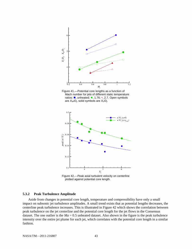
NASA/TM—2011-216807 43

Figure 41.—Potential core lengths as a function of

Mach number for jets of different static temperature ratios: , unheated; , 1.76; , 2.7. Open symbols are XW/Dj, solid symbols are Xc/Dj.

Figure 42.—Peak axial turbulent velocity on centerline

plotted against potential core length.

5.3.2 Peak Turbulence Amplitude Aside from changes in potential core length, temperature and compressibility have only a small

impact on subsonic jet turbulence amplitudes. A small trend exists that as potential lengths decreases, the centerline peak turbulence increases. This is illustrated in Figure 42 which shows the correlation between peak turbulence on the jet centerline and the potential core length for the jet flows in the Consensus dataset. The one outlier is the Ma = 0.5 unheated dataset. Also shown in the figure is the peak turbulence intensity over the entire jet plume for each jet, which correlates with the potential core length in a similar fashion.

NASA/TM—2011-216807 44

5.3.3 Jet Spread While the potential core length is an important normalizing factor in jets, it is not the only difference

caused by temperature and compressibility. The radial spread of the jet and the exponential decay region are also influenced in subtle ways that can be seen in this carefully cleaned data. In Figure 43 contour plots of the seven jet flow fields are overlaid, normalizing the axial coordinate by the experimentally obtained potential core length Xc. Examination of the plots reveals that, although the potential core lengths of all the datasets are the same by virtue of the normalization with Xc, the contours group by static temperature ratio or density. (Note that the line colors in the contour plots have been chosen to group jets with the same temperature ratio.) The unheated jets have a much greater spread rate than the heated jets and decay at a lower rate downstream. The grouping by static temperature ratio is a clear indication that it is density which drives these aspects of the flow, not the Mach number or compressibility: e.g., setpoints 23, 27, and 29 have aerodynamic Mach numbers Mj = 0.38, 0.9, 1.0 while maintaining the same static temperature ratio. The peak turbulence levels and their location are similarly affected by temperature, not Mach number. In Figure 43 the contour lines for a given turbulence level occur farther downstream and closer to the centerline with increased temperature.

Perhaps a more direct way of seeing the impact of temperature is to look at radial profiles at given fractions of the potential core length. From these plots in Figure 44 it becomes apparent how the peak location of the turbulence tracks with the max shear of the mean velocity profiles, causing the turbulence to peak in the cold jets further away from the centerline than in the hot jets.

Figure 43.—Mean and turbulent axial velocity contours for the seven consensus datasets, plotted with axial

coordinate normalized by experimentally determined potential core length.

NASA/TM—2011-216807 45

Figure 44.—Radial profiles of consensus data for all setpoints at axial stations relative to potential core length Xc.

Profiles plotted at x/Xc = 0.5, 1.0, 1.5, 2.0. The classic shear layer parameters of half-velocity point r0.5 and shear layer thickness δω were

calculated for each profile and are presented in Figure 45. The shear layer parameters were compared with those results published in Lau (Ref. 10). It appears that the Consensus data is a bit more self-consistent, but the general trends on change with Mach number and temperature ratio agree between the two datasets. As noted above, neither the half-velocity radius nor the shear layer thickness is a strong function of Mj, but only of temperature. These statistics were obtained for the streamwise location x = Xc, which is probably as far downstream as one can expect the jet shear layer to be approximately two-dimensional. Converting these parameters to growth rates, e.g., dividing the parameters by the axial distance, assuming this rate to be constant, one obtains the divergence angle of the half-velocity point ψ = (r0.5 – Dj/2)/x and the growth in the shear layer thickness δω/x. These are given in Figure 46, again as a function of both temperature ratio and Mach number. From these plots it is seen that the jet spread ψ varies considerably with temperature, but not Mach number. The spread rate δω/x, on the other hand, has some dependence on Mach number, but not temperature ratio. When plotted against Mach number Mj the spread rate measured in the Consensus PIV datasets fall along a single line, relatively independent of temperature ratio. The data of Lau has similar trends, but has a 10 percent greater spread rate than the Consensus data, and the data at the highest temperature (Tj/T∞ = 2.32) does not fall in with the data of the two other temperature ratios.

NASA/TM—2011-216807 46

Figure 45.—Shear layer parameters r0.5 (jet half-width) and δω (shear layer thickness) as reported in Lau (Ref. 10)

and in Consensus datasets. Plots show dependence on static temperature ratio Tj/T∞ and on Mj for x = Xc.

Figure 46.—Shear layer growth parameters ψ (jet half-width) and δωx (shear layer thickness) with downstream

distance as reported in Lau (Ref. 10) and in Consensus datasets. Plots show dependence on static temperature ratio Tj/T∞ and on Mj.

NASA/TM—2011-216807 47

Figure 47.—Mean and turbulent axial velocity contours for the seven consensus datasets, plotted with axial

coordinate normalized by experimentally determined potential core length and transverse coordinate normalized to unify jet spread (half-velocity point).

5.3.4 Combined Rescaling of Jet Having determined appropriate streamwise scaling from consideration of potential core length, and

the shear layer scaling in terms of half-width and shear layer thickness, the contour plots of mean and turbulence velocity from all seven Consensus datasets are rescaled and overlaid as shown in Figure 47. The choice of streamwise coordinate is obvious, but the radial coordinate is not as straightforward. Using the standard shear layer coordinates η is inappropriate because it does not preserve the jet axis. The cross-stream coordinate y/Yc used in the figure is essentially a simple radial stretch which maps the half-velocity radius to the lipline of the jet. No consideration of the shear layer thickness is required—the shear layer thickness scales relatively well without it when the streamwise coordinate is scaled by the potential core. This self-consistency shown in Figure 47 provides strong support both of traditional turbulence theory that gives rise to the normalization of shear layers, and of the Consensus datasets. The main area of disagreement is in the peak levels of the unheated jet, which are significantly lower than the other jets. The cause of this difference is not apparent at this time.

6.0 Summary A large body of Particle Image Velocimetry (PIV) data has been acquired over eight years of testing

with different installations of optics and different generations of processing. Several flow cases covering a range of shock-free jets with different temperatures were repeatedly measured. The number of different test configurations and setups has produced opportunities to remove many bias errors associated with PIV configuration and the shear number of measurements reduces the random errors. Careful operation, including proper seeding techniques and close monitoring of flow conditions has also contributed to the high quality of the data.

This report details the experimental facility and the nozzle model hardware, including studies of the initial shear layer characteristics. It further covers all details of the PIV equipment, operations, and analysis during each test entry. It includes an extensive literature survey comparing turbulence data from many sources using different anemometry techniques. A subset of these data were chosen and justified for comparisons with the PIV datasets for cases of low subsonic cold, high subsonic cold, and high subsonic hot jets. This comparison provided an estimate of the bias error in the PIV data, e.g., the error that all the

NASA/TM—2011-216807 48

PIV data shared. It was found that the PIV turbulence intensity measurements fell within the 7 percent spread of the literature sources for the low subsonic cold jet with no appreciable bias, and within the 12 percent spread of the high subsonic cold jet with just a small bias to higher amplitudes if one does not include the LDV data sources from the literature. Very little basic turbulence data exists for high-speed jets and even less for high-speed hot jets. When the PIV data was overlaid on this data no appreciable bias was found.

A process of weighing, averaging, and smoothing the data from all the test entries was documented and used to obtain a ‘Consensus’ dataset for each flow case. The main objective of this Consensus dataset was to provide data for CFD validation and for studying subtle trends in the jet scaling, along with estimates of the uncertainty in the data. This dataset is intended to embody the best judgment of the experimentalist, freeing the end user from interpreting data irregularities. The raw data from all test entries were plotted along with the final Consensus dataset to establish random error estimates for the Consensus datasets.

Finally, the Consensus dataset was analyzed and standard characteristic measures of jets were compared with values from the literature. Potential core lengths, jet half-widths, peak turbulence levels, and shear layer growth rates were computed and compared with previous studies made using laser Doppler velocimetry. When the shear layer data for all jet flow cases were normalized using these appropriate parameters, the data from all flow cases collapsed in a satisfying manner.

References

1. Laurence, J.C., “Intensity, Scale, and Spectra of Turbulence In Mixing Regions of Free Subsonic Jet,” NACA Report 1292 (1956).

2. Davies, P.O.A.L., Fisher M.J. and Barratt, M.J., “The characteristics of the turbulence in the mixing region of a round jet,” J. Fluid Mech. 15, 337 (1963).

3. Fisher, M. J. and Davies, P. O. A. L. “Correlation measurements in a non-frozen pattern of turbulence,” J. Fluid Mech. 18, 97 (1964).

4. Bradshaw, P., Ferriss, D.H. and Johnson, R.F., “Turbulence in the noise-producing region of a circular jet,” J. Fluid Mech. 19, 591 (1964).

5. Ko, N.W.M. and Davies, P.O.A.L., “The near field within the potential cone of subsonic cold jets,” J. Fluid Mech. 60, 49 (1971).

6. Crow, S.C., and Champagne, F.H., “Orderly structure in jet turbulence,” J. Fluid Mech. 48, 547 (1971).

7. Raman, G., Zaman, K.B.M.Q., and Rice, E.J., “Initial turbulence effect on jet evolution with and without tonal excitation,” Phys Fluids A 1 1240 (1978).

8. Lau, J.C., Morris, P.J. and Fisher, M.J., “Measurements in subsonic and supersonic free jets using a laser velocimeter,” J. Fluid Mech. 93, 1 (1979).

9. Lau, J.C., “Laser velocimeter correlation measurements in subsonic and supersonic jets,” J Sound Vibration 70, 85 (1980).

10. Lau, J.C., “Effects of exit Mach number and temperature on mean-flow and turbulence characteristics in round jets,” J. Fluid Mech. 105, 193 (1981).

11. Ahuja, K.K., Lepicovsky, J., Tam, C.K.W., Morris, P.J., and Burrin, R.H. “Tone-excited jet: Theory and experiments,” NASA CR–3538 (1982).

12. Zaman, K.B.M.Q., Wang, F.Y., and Georgiadis, N.J., “Noise, turbulence, and thrust of subsonic freejets from lobed nozzles,” AIAA J., 41, 398 (2003).

13. Kerherve, F., Jordan, P., Gervais, Y., Valiere, J.-C., and Braud, P., “Two-point laser Doppler velocimetry measurements in a Mach 1.2 cold supersonic jet for statistical aeroacoustic source model,” Expt Fluids 37, 419 (2004).

14. Morris, P.J. and Zaman, K.B.M.Q., “Velocity measurements in jets with application to noise source modeling,” AIAA Paper 2009-17 (2009).

NASA/TM—2011-216807 49

15. Pokora, C.D. and McGuirk, J.J., “Spatio-Temporal Turbulence Correlations using High-Speed PIV in an Axisymmetric Jet,” AIAA–2008–3028, (2008).

16. Witze, P.O., “Centerline velocity decay of compressible free jets,” AIAA J 12, 417 (1974). 17. Viswanathan. K. “Jet aeroacoustic testing: issues and implications,” AIAA J 41, 1674 (2003). 18. Ahuja. K.K., “Designing clean jet-noise facilities and making accurate jet-noise measurements,” Intl

J. Aeroacoustics 2, 314 (2003). 19. Brown, C.A., and Bridges, J., “Small Hot Jet Acoustic Rig Validation,” NASA TM—2006/214234

(2006). 20. Plumblee, H.E., Burrin, R.H., Lau, J.C., Morfey, C.L. Morris, P.J., Smith, D.M., Tanna, H.K., Tester,

B.J., Whiffen, M.C., “The generation and radiation of supersonic jet noise, part III, Turbulent mixing noise data,” AFAPL–TR–76–45, 1976.

21. Bridges, J., “Effect of Heat on Space-Time Correlations in Jets,” AIAA–2006–2534 (2006). 22. Bridges, J. and Wernet, M.P., “Effect of Temperature on Jet Velocity Spectra,” AIAA–2007–3628,

(2007). 23. Bridges. J. and Wernet, M.P., “Measurements of the aeroacoustic sound source in hot jets,” AIAA–

2003–3130, (2003). 24. Opalski, A.B., Wernet, M.P., and Bridges, J., “Chevron nozzle performance characterization using

stereoscopic DPIV,” AIAA– 2005–0444, (2005). 25. Bjorkquist, D.C., “Design and calibration of a stereoscopic PIV system,” Proc. 9th International

Symposium on Applications of Laser Techniques to Fluid Mechanics, Vol. 1, 6.5.1, Lisbon, Portugal (1998).

26. Soloff, S.M., Adrian, R.J., and Liu, Z-C, “Distortion Compensation for Generalized Stereoscopic Particle Image Velocimetry,” Measurement Science and Technology 8, 1441, (1997).

27. Wernet, M.P., “Fuzzy Logic Enhanced Digital PIV Processing Software,” NASA TM—1999/209274, (1999).

28. Wernet, M.P., Skoch, G.J., and Wernet, J.H., “Demonstration of a Stabilized Alumina/Ethanol Colloidal Dispersion Technique for Seeding High Temperature Air Flows,” 16th International Congress on Instrumentation for Aerospace Simulation Facilities (ICIASF), (1995).

REPORT DOCUMENTATION PAGE Form Approved OMB No. 0704-0188

The public reporting burden for this collection of information is estimated to average 1 hour per response, including the time for reviewing instructions, searching existing data sources, gathering and maintaining the data needed, and completing and reviewing the collection of information. Send comments regarding this burden estimate or any other aspect of this collection of information, including suggestions for reducing this burden, to Department of Defense, Washington Headquarters Services, Directorate for Information Operations and Reports (0704-0188), 1215 Jefferson Davis Highway, Suite 1204, Arlington, VA 22202-4302. Respondents should be aware that notwithstanding any other provision of law, no person shall be subject to any penalty for failing to comply with a collection of information if it does not display a currently valid OMB control number. PLEASE DO NOT RETURN YOUR FORM TO THE ABOVE ADDRESS. 1. REPORT DATE (DD-MM-YYYY) 01-11-2011

2. REPORT TYPE Technical Memorandum

3. DATES COVERED (From - To)

4. TITLE AND SUBTITLE The NASA Subsonic Jet Particle Image Velocimetry (PIV) Dataset

5a. CONTRACT NUMBER

5b. GRANT NUMBER

5c. PROGRAM ELEMENT NUMBER

6. AUTHOR(S) Bridges, James; Wernet, Mark, P.

5d. PROJECT NUMBER

5e. TASK NUMBER

5f. WORK UNIT NUMBER WBS 984754.02.07.03.17.03

7. PERFORMING ORGANIZATION NAME(S) AND ADDRESS(ES) National Aeronautics and Space Administration John H. Glenn Research Center at Lewis Field Cleveland, Ohio 44135-3191

8. PERFORMING ORGANIZATION REPORT NUMBER E-17439

9. SPONSORING/MONITORING AGENCY NAME(S) AND ADDRESS(ES) National Aeronautics and Space Administration Washington, DC 20546-0001

10. SPONSORING/MONITOR'S ACRONYM(S) NASA

11. SPONSORING/MONITORING REPORT NUMBER NASA/TM-2011-216807

12. DISTRIBUTION/AVAILABILITY STATEMENT Unclassified-Unlimited Subject Categories: 07 and 34 Available electronically at http://www.sti.nasa.gov This publication is available from the NASA Center for AeroSpace Information, 443-757-5802

13. SUPPLEMENTARY NOTES

14. ABSTRACT Many tasks in fluids engineering require prediction of turbulence of jet flows. The present document documents the single-point statistics of velocity, mean and variance, of cold and hot jet flows. The jet velocities ranged from 0.5 to 1.4 times the ambient speed of sound, and temperatures ranged from unheated to static temperature ratio 2.7. Further, the report assesses the accuracies of the data, e.g., establish uncertainties for the data. This paper covers the following five tasks: (1) Document acquisition and processing procedures used to create the particle image velocimetry (PIV) datasets. (2) Compare PIV data with hotwire and laser Doppler velocimetry (LDV) data published in the open literature. (3) Compare different datasets acquired at the same flow conditions in multiple tests to establish uncertainties. (4) Create a ‘consensus’ dataset for a range of hot jet flows, including uncertainty bands. (5) Analyze this consensus dataset for self-consistency and compare jet characteristics to those of the open literature. The final objective was fulfilled by using the potential core length and the spread rate of the half-velocity radius to collapse of the mean and turbulent velocity fields over the first 20 jet diameters. 15. SUBJECT TERMS Computational fluid dynamics; Jet flow; Turbulence; Turbulent jets; Statistical analysis; Aeroacoustics; Noise prediction; Flow characteristics; Reynolds stress 16. SECURITY CLASSIFICATION OF: 17. LIMITATION OF

ABSTRACT UU

18. NUMBER OF PAGES

56

19a. NAME OF RESPONSIBLE PERSON STI Help Desk (email:[email protected])

a. REPORT U

b. ABSTRACT U

c. THIS PAGE U

19b. TELEPHONE NUMBER (include area code) 443-757-5802

Standard Form 298 (Rev. 8-98)Prescribed by ANSI Std. Z39-18

The NASA Subsonic Jet Particle Image Velocimetry (PIV) Dataset · 2013-04-10 ·...

Documents

Transcript of The NASA Subsonic Jet Particle Image Velocimetry (PIV) Dataset · 2013-04-10 ·...