179

Chapter 9

OVERVIEW OF PART II:THE ANALYSIS OF 1996 NAEP DATA1

Nancy L. Allen and James E. CarlsonEducational Testing Service

9.1 INTRODUCTION

The purpose of this chapter is to summarize some information from previous chapters that isintegral to the analysis of NAEP data, to summarize the analysis steps used for all subjects, and toindicate what information is in each of the remaining chapters. The overview of the analyses conductedon the 1996 NAEP data focuses on the common elements of the analyses used across the subject areas ofthe assessment. Some of this information is available only within this chapter. Details by subject area areprovided in Chapters 12 through 17.

The organization of this chapter is as follows:

• Section 9.2 provides a short overview of the NAEP design for 1996. To provideadditional background information, the section also provides a short description ofthe samples selected for 1996. Chapters 1 through 8 provide this same information inmuch more detail.

• Section 9.3 summarizes the steps in analysis common to all subject areas. Some of

this information is described in more detail in other chapters. The rest is includedonly within this chapter. The topics covered are as follows:

• Section 9.3.1 briefly describes the preparation of the final sampling weights.

Detailed information about the weighting procedures is given in Chapter 10. Detailedinformation about the sampling design is in Chapter 3.

• Section 9.3.2 provides information about the scoring reliability of constructed-

response items. It provides information about the reliability measures used with theNAEP data during analysis. Chapter 7 contains information about the reliabilityprocedures used during the scoring process.

• Section 9.3.3 summarizes the information provided by the teacher questionnaires,

and indicates its use during the analysis process. • Section 9.3.4 provides a description of the item properties examined for background

questions and for cognitive items. It includes a description of the classical itemstatistics examined for both dichotomously and polytomously scored items. It also

1 Nancy L. Allen was responsible for the psychometric and statistical analyses of national and state NAEP data. James E. Carlsonwas responsible for psychometric and statistical analyses relating to special aspects and issues of NAEP. Eugene G. Johnson,John Mazzeo, Spencer S. Swinton, and Rebecca Zwick also contributed to this chapter.

180

includes a description of the item-level results available from summary data tables.Chapter 18 contains more information about the conventions used in creating thesesummary tables. Finally, a thorough description of differential item functioninganalyses is provided.

• Section 9.3.5 summarizes the steps used to scale NAEP data. The steps include IRT

scaling of the items, generation of plausible values (conditioning), transforming theresults to the final reporting scale, creating composite scores if necessary, andproviding tables of reported statistics. Details of the theory behind these steps areavailable in Chapter 11.

• Section 9.3.6 provides some information about previous results of dimensionality

analyses. • Finally, Section 9.3.7 gives an introduction to hypothesis testing and drawing correct

conclusions about NAEP data. Specific information about which hypothesis testprocedures were used for different purposes is provided in Chapter 18.

• Section 9.4 contains a description of the information provided in Chapters 10

through 19 of this report.

9.2 SUMMARY OF THE NAEP DESIGN

As described in Chapter 1, the 1996 NAEP comprised three major components. One componentencompassed major assessments in mathematics and science, providing detailed information aboutstudent proficiency at the fourth-, eighth-, and twelfth-grade levels of nonpublic and public schools.Long-term trend assessments of science, mathematics, and reading at ages 9, 13, and 17, and the long-term trend writing assessment for grades 4, 8, and 11, constituted the second component. The third majorcomponent was the State Assessment at the fourth- and eighth-grade levels in mathematics and at theeighth-grade level in science. Technical details of the State Assessments are not included in this reportbut are presented in the Technical Report of the NAEP 1996 State Assessment Program in Mathematics(Allen, Jenkins, Kulick, & Zelenak, 1997) and the Technical Report of the NAEP 1996 State AssessmentProgram in Science (Allen, Swinton, Isham, & Zelenak, 1997).

In addition to the three major components, special studies of advanced mathematics students atthe eighth- and twelfth-grade levels and advanced science students at the twelfth-grade level wereconducted. The results from and procedures used in these special studies are reported in separatedocuments. Likewise, results from a study of holistic scores for the long-term trend writing taskresponses are reported in a separate document. Results based on primary trait scores for the same writingtasks are reported in the NAEP 1996 Trends in Academic Progress (Campbell, Voelkl, & Donahue,1997), and the analyses contributing to those results are described in Chapters 14-17 of this document.Finally, results for the items associated with specific mathematics themes are reported elsewhere.

Results from the analyses described in the following chapters were reported in the followingreports:

• The NAEP 1996 Mathematics Report Card for the Nation and the States, whichprovides both public- and nonpublic-school data for major NAEP reporting

181

subgroups for all of the jurisdictions that participated in the State Assessment program, aswell as selected results from the 1996 national mathematics assessment.

• The NAEP 1996 Science Report Card for the Nation and the States, which provides both

public- and nonpublic-school data for major NAEP reporting subgroups for all of thejurisdictions that participated in the State Assessment program, as well as selected resultsfrom the 1996 national science assessment.

• The Cross-State Data Compendium for the NAEP 1996 Mathematics Assessment, which

includes jurisdiction-level results for all the demographic, instructional, and experientialbackground variables included in the Mathematics Report Card and State Reports.

• The Cross-State Data Compendium for the NAEP 1996 Science Assessment, whichincludes jurisdiction-level results for all the demographic, instructional, and experientialbackground variables included in the Science Report Card and State Reports.

• The NAEP 1996 Trends in Academic Progress, which looks at trends in averageperformance over time in the areas of mathematics, science, reading, and writing. [Pleasenote that a review of the 1996 long-term trend writing assessment data analyses has beenundertaken by NCES. Additional analyses may be required before revised results arereleased.]

Because the samples of students included in the 1996 NAEP assessment are listed and described indetail in Chapter 1, only a brief description of these samples is given here. The 1996 national samples wereof three general types: main NAEP samples, which were based on a common set of assessment procedures,including grade-level samples; long-term trend samples, the purpose of which was to provide links toearlier assessments; and special study samples, used to examine results for advanced mathematics andscience students.

To shorten the timetable for reporting results, the period for national main assessment datacollection was shortened in 1992, 1994, and 1996 from the five-month period (January through May) usedin 1990 and earlier assessments to a three-month period in the winter (January through March,corresponding to the period used for the winter half-sample of the 1990 National Assessment). [Please notethat a review of the 1996 long-term trend writing assessment data analyses has been undertaken by NCES.Additional analyses may be required before revised results are released.]

The 1996 analyses of long-term trend data extended the trend lines commencing in 1971 inreading, 1973 in mathematics, 1969 in science, and 1984 in writing.

As described in Chapters 1 and 4, for each subject area in the main assessment, blocks of itemswere used to create a large number of different assessment booklets according to a focused design. The1996 mathematics assessment used a focused balanced incomplete block (focused-BIB) design while the1996 science assessment used a more complex design due to the inclusion of blocks of items associatedwith a specific theme or hands-on performance task. The focused-BIB design provided for booklets thattypically included three blocks of cognitive items in a single subject area, as well as background items. Theblocks of cognitive items for mathematics and science included both multiple-choice and constructed-response items. In a focused-BIB design, each block of cognitive items appears in the same number ofbooklets. To balance possible block position main effects, each block appears an equal number of times ineach position. In addition, the BIB design requires that each block of items be paired in a booklet withevery other block of items exactly once.

182

9.3 ANALYSIS STEPS

Because the analysis methods are not identical across subject areas or across major national andlong-term trend samples, a separate analysis chapter has been included for each major assessment and foreach long-term trend assessment. The procedures used depended on whether assessment items werescored dichotomously (right versus wrong) or polytomously (more than two categories of response) andwhether links across grade levels were required. Basic procedures common to most or all of the subjectarea analyses are summarized here. The order is essentially that in which the procedures were carried out.

9.3.1 Preparation of Final Sampling Weights

Because NAEP uses a complex sampling design (Chapter 3) in which students in certainsubpopulations have different probabilities of inclusion in the sample, the data collected from eachstudent must be assigned a weight to be used in analyses. The 1996 NAEP weights were provided byWestat, Inc., the NAEP contractor in charge of sampling. Detailed information about the weightingprocedures is available in Chapter 10 and in The 1996 NAEP Sampling and Weighting Report (Wallace &Rust, 1999).

9.3.2 Reliability of Scoring Constructed-Response Items

A minimum of 25 percent of the responses for science items involved only in the nationalassessment and six percent of the responses for mathematics and science items involved in both thenational and state assessments were scored by a second reader to obtain statistics on interreader(interrater) reliability. Ranges for percentage of exact agreement for state and national assessments,together, of mathematics and science can be found in Table 9-1. Average percentage of exact agreementfor each booklet type (spiral and advanced) can be found in Tables 7-5 and 7-6 in Chapter 7. Thisreliability information was also used by the team leaders to monitor the capabilities of all readers andmaintain uniformity of scoring across readers. More information about this use of the reliabilityinformation is in Chapter 7.

Table 9-11996 Mathematics and Science State and National Assessments

Ranges of Percentage Exact Agreement Among Readers

Number ofUnique Items

Number of Items in PercentageExact Agreement Range

Assessment Total 70-79% 80-89% Above 90%Mathematics

4th grade 79 0 11 688th grade 98 1 5 9212th grade 96 1 9 86

Science4th grade 94 0 13 818th grade 125 0 20 10512th grade 156 0 26 130

183

In addition to reliability information calculated and used during the scoring process, severaladditional reliability measures are calculated for constructed-response items after the item response datahas been placed on the NAEP database. They appear in Appendix I. These include a final percentageexact agreement, the intraclass correlation, Cohen’s Kappa (Cohen, 1968), and the product-momentcorrelation between the scores for the first and second readers. These measures are summarized in Zwick(1988), Kaplan and Johnson (1992), and Abedi (1996). Each measure has advantages and disadvantagesfor use in different situations. In this report, the percentage exact agreement is reported for allconstructed-response items, Cohen’s Kappa is reported for dichotomously scored constructed-responseitems, and the intraclass correlation is reported for polytomously scored constructed-response items.

9.3.3 Teacher Questionnaires

Teachers of students who were in the fourth- and eighth-grade mathematics and science mainassessment samples and twelfth-grade advanced mathematics samples were asked to complete a two-partquestionnaire. The first part of the questionnaire pertained to the teacher’s background and training(Parts I and IIA in Chapter 2). The second part pertained to the procedures used by the teacher forspecific classes containing assessed students (Part IIB in Chapter 2). See Chapter 2 for a description ofthe teacher questionnaires.

To analyze the data from the teacher questionnaires with respect to the students’ data, eachteacher’s questionnaire had to be matched to all of the sampled students who were taught by that teacher.In the subsequent chapters two separate match rates for each grade are given. The first is the percentageof students that could be matched to both the first and second parts of the teacher questionnaire. For thesestudents, information is available not only about the background and training of their teachers, but alsoabout the methods used in the particular class they attended. The second match rate is the percentage ofstudents that could be matched to the first part of the teacher questionnaire. This match rate is largerbecause more students could be matched with information about a teacher than with information aboutthe particular class they attended. Note that these match rates only reflect the student-level missing data.They do not reflect the additional missing data due to item-level nonresponse on the part of teachers.Variables derived from the teacher questionnaires were used as reporting variables at the student leveland as variables that contributed to conditioning for the appropriate samples.

Teachers of students who were in the grade 4 mathematics main assessment sample were askedto complete a two-part questionnaire. As with the grade 8 teacher questionnaire, the first part pertained tothe teacher’s background and training. Unlike the grade 8 teacher questionnaire, the second partpertained to only a single class that the teacher taught. In development of the questionnaires, it wasthought that fourth-grade teachers would teach one class in each subject. In practice, that was found to beuntrue for a number of teachers. A single student-teacher match rate matching students to the first part ofthe questionnaire is reported for grade 4 in the following chapters.

9.3.4 Analysis of Item Properties: Background and Cognitive Items

The first step in the analysis of the 1996 data was item-level analysis of all instruments. Itemanalyses were performed separately for each grade or age level on each item in each subject area. Eachblock of items was analyzed separately, by age or grade, with the total score on the block (including theanalyzed item) used as the criterion score for statistics requiring such a score. In the cases where finalweights were not available, preliminary weights were used in these preliminary analyses. The item

184

analysis of cognitive items was repeated after scaling of the items was completed. The results for onlyscaled items using final weights are reported in Chapters 12 through 17.

� Background Items

For each NAEP background item, the unweighted and weighted percent of students who gaveeach response were examined, as well as the percent of students who omitted the item and the percentwho did not reach the item. The number of respondents was also tabulated. These preliminary analyseswere conducted within age/grade cohorts and within major reporting categories. If unexpected resultswere found, the item data and the encoding of responses were rechecked.

� Cognitive Items

All NAEP cognitive items were subjected to analyses of item properties. These analyses includedconventional item analyses and incorporated examinee sampling weights. Item analysis was conducted atthe block level so that the “number-correct” scores for students responding to an item, selecting eachoption of an item, omitting an item, or not reaching an item, is the average number of correct responsesfor the block containing that item. Because of the inclusion of polytomously scored items in the cognitiveinstruments, it was necessary to use special procedures for these items. The resulting statistics areanalogous to those for the dichotomously scored items, as listed below.

Dichotomously Scored Items. These items were analyzed using standard procedures that resultin a report for each item that includes:

� for each option of the item, for examinees omitting and not reaching the item, and forthe total sample of examinees:

⇒ the number of examinees,

⇒ the percentage of examinees,

⇒ the mean of number-correct scores for the block in which the item appears, and

⇒ the standard deviation of number-correct scores for the block in which the itemappears;

• the percentage of examinees providing a response that was “off-task;” • p+, the proportion of examinees that received a correct score on the item (ratio of

number correct to number correct plus wrong plus omitted);

• �, the inverse-normally transformed p+ scaled to mean 13 and standard deviation 4;

• the biserial correlation coefficient between the item and the number-correct scoresfor the block in which the item appears; and

• the point-biserial correlation coefficient between the item and the number-correct

scores for the block in which the item appears.

185

Polytomously Scored Items. Enhanced procedures were employed for polytomously scoreditems. Methods parallel to those used for dichotomously scored items resulted in values reported for eachdistinct response category for the item. Response categories for each item were defined in two ways, onebased on the original codes for responses as specified in the scoring rubrics used by the scorers (and theposition of the item for which no response was given) and one based on a scoring guide developed bysubject area and measurement experts. For example, a constructed-response item with four responsecategories would initially have seven categories (not-reached, omitted, “off-task,” and the four validresponse categories). Another set of statistics resulted from mapping the response categories (excludingnot-reached) into a new set of categories reflecting the scoring guide for the item. A constructed-responseitem with ordered categories, for example, would be mapped into a set of integers in a correspondingorder. The scoring guide could result in the collapsing of (combining of) some response categories. Theresponse categories, based on the final scoring guide developed by subject area and measurement experts,were used to calculate the polytomously scored item statistics.

The following statistics, analogous to those for dichotomously scored items, were computed:

• the percentage of examinees providing a response that was “off-task;” • in place of p+, the ratio of the mean item score to the maximum-possible item score

was used;

• in place of �, the ratio of the mean item score to the maximum-possible item scoreunderwent the same transformation as that used on p+ to get � for dichotomouslyscored items;

• the polyserial correlation coefficient was used in place of the biserial; and

• the Pearson correlation coefficient was used in place of the point-biserial.

� Tables of Item-Level Results

Tables were created of the percentages of students choosing each of the possible responses toeach item within each of the samples administered in 1996. The results for each item were cross-tabulated against the basic reporting variables such as region, gender, race/ethnicity, public/nonpublicschool, and parental education. All percentages were computed using the sampling weights. These tablesare referred to as the Test Question section of the electronically delivered summary data tables for eachsample (see Chapter 18 for a brief description of summary data tables). In the summary data tables, thesampling variability of all population estimates was obtained by the jackknife procedure used by ETS inprevious assessments. Details of these procedures are presented in Chapter 10.

� Differential Item Functioning Analysis of Cognitive Items

Differential item functioning (DIF) analysis refers to procedures to assess whether items aredifferentially difficult for different groups of examinees. DIF procedures typically control for overallbetween-group differences on a criterion, usually by matching examinees from the two groups on overalltest scores. Between-group performance on each item is then compared within sets of examinees havingthe same total test scores.

186

DIF analyses were conducted for items in the main assessments in mathematics and science thathad not previously been studied for differential item functioning. Each set of analyses involved threereference group/focal group comparisons: male/female, White/Black, and White/Hispanic.

The DIF analyses of the dichotomous items were based on the Mantel-Haenszel chi-squareprocedure, as adapted by Holland and Thayer (1988). The procedure tests the statistical hypothesis thatthe odds of correctly answering an item are the same for two groups of examinees that have beenmatched on some measure of proficiency (usually referred to as the matching criterion). The DIFanalyses of the polytomous items were based on the Mantel procedure (Mantel, 1963). These procedurescompare proportions of matched examinees from each group in each polytomous item response category.The groups being compared are often referred to as the focal group (usually a minority or other group ofinterest, such as Black examinees or female examinees) and the reference group (usually Whiteexaminees or male examinees).

For both types of analyses, the measure of proficiency used is typically the total item score onsome collection of items. Since, by the nature of the BIB design, booklets comprise differentcombinations of blocks, there is no single set of items common to all examinees. Therefore, for eachstudent, the measure of proficiency used was the total item score on the entire booklet. These scores werethen pooled across booklets for each analysis. This procedure is described by Allen and Donoghue (1994,1996). In addition, because research results (Zwick & Grima, 1991) strongly suggest that samplingweights should be used in conducting DIF analyses, the weights were used.

For each dichotomous item in the assessment, an estimate of the Mantel-Haenszel common odds-ratio, expressed on the ETS delta scale for item difficulty, was produced. The estimates indicate thedifference between reference group and focal group item difficulties (measured in ETS delta scale units),and typically run between about +3 and -3. Positive values indicate items that are differentially easier forthe focal group than the reference group after making an adjustment for the overall level of proficiency inthe two groups. Similarly, negative values indicate items that are differentially harder for the focal groupthan the reference group. It is common practice at ETS to categorize each item into one of threecategories (Petersen, 1988): “A” (items exhibiting no DIF), “B” (items exhibiting a weak indication ofDIF), or “C” (items exhibiting a strong indication of DIF). Items in category “A” have Mantel-Haenszelcommon odds ratios on the delta scale that do not differ significantly from 0 at the alpha = .05 level orare less than 1.0 in absolute value. Category “C” items are those with Mantel-Haenszel values that aresignificantly greater than 1 and larger than 1.5 in absolute magnitude. Other items are categorized as “B”items. A plus sign (+) indicates that items are differentially easier for the focal group; a minus sign (-)indicates that items are differentially more difficult for the focal group.

The ETS/NAEP DIF procedure for polytomous items uses the Mantel-Haenszel ordinalprocedure. The summary tables of identified polytomous items contain generalizations of thedichotomous “A,” “B,” and “C” categories: “AA,” “BB,” or “CC.”

All analyses used rescaled sampling weights. A separate rescaled weight was defined for eachcomparison as

where the total sample size is the total number of students for the two groups being analyzed (e.g., for theWhite/Hispanic comparison, the total number of White and Hispanic examinees in the sample at thatgrade), and the sum of the weights is the sum of the sampling weights of all the students in the sample for

Rescaled Weight = Original Weight x Total Sample Size

Sum of the Weights

187

the two groups being analyzed. Three rescaled weights were computed for White examinees one for thegender comparison and two for the race/ethnicity comparisons. Two rescaled overall weights werecomputed for the Black and Hispanic examinees��one for the gender comparison and another for theappropriate race/ethnicity comparison. The rescaled weights were used to ensure that the sum of theweights for each analysis equaled the number of students in that comparison, thus providing an accuratebasis for significance testing.

In the calculation of total item scores for the matching criterion, both not-reached and omitteditems were considered to be wrong responses. Polytomous items were weighted more heavily in theformation of the matching criterion, proportional to the number of score categories. For each item,calculation of the Mantel-Haenszel statistic did not include data from examinees who did not reach theitem in question.

Each DIF analysis was a two-step process. In the initial phase, total item scores were formed, andthe calculation of DIF indices was completed. Before the second phase, the matching criterion wasrefined by removing all “C” or “CC” items, if any, from the total item score. The revised score was usedin the final calculation of all DIF indices. Note that when analyzing an item classified as “C” or “CC” inthe initial phase, that item score is added back into the total score for the analysis of that item only.

Following standard practice at ETS for DIF analyses conducted on final forms, all “C” or “CC”items were reviewed by a committee of trained test developers and subject-matter specialists. Suchcommittees are charged with making judgments about whether or not the differential difficulty of an itemis unfairly related to group membership. The committee assembled to review NAEP items included bothETS staff and outside members with expertise in the field. The committee carefully examined eachidentified item to determine if either the language or contents would tend to make the item more difficultfor an identified group of examinees. It was the committee’s judgment that none of the “C” or “CC”items in the national assessment were functioning differentially due to factors irrelevant to testobjectives. Hence, none of the items were removed from scaling due to differential item functioning. Aspointed out by Zieky (1993):

It is important to realize that DIF is not a synonym for bias. The item response theory basedmethods, as well as the Mantel-Haenszel and standardization methods of DIF detection, will identifyquestions that are not measuring the same dimension(s) as the bulk of the items in the matchingcriterion....Therefore, judgment is required to determine whether or not the difference in difficultyshown by a DIF index is unfairly related to group membership. The judgment of fairness is based onwhether or not the difference in difficulty is believed to be related to the construct beingmeasured....The fairness of an item depends directly on the purpose for which a test is being used.For example, a science item that is differentially difficult for women may be judged to be fair in atest designed for certification of science teachers because the item measures a topic that every entry-level science teacher should know. However, that same item, with the same DIF value, may bejudged to be unfair in a test of general knowledge designed for all entry-level teachers. (p. 340)

9.3.5 Scaling

Scales based on item response theory (IRT) were derived for each subject area. A single scalewas used for summarizing long-term trends at each age or grade level in each of the subject areas. Fivescales were created for mathematics main assessment data, one for each mathematics content strand, andthree scales were created for science data, one for each field of science. NAEP uses the methodology ofmultiple imputations (plausible values) to estimate characteristics of the proficiency distributions.

188

Chapter 11 describes in detail the theoretical underpinnings of NAEP’s scaling methods and the requiredestimation procedures. The basic analysis steps are outlined here.

1. Use the NAEP-BILOG/PARSCALE computer program (described in Chapter 11) toestimate the parameters of the item response functions on an arbitrary provisionalscale. This program uses an IRT model incorporating the two- and three-parameterlogistic forms used in previous assessments for dichotomously scored items and thegeneralized partial credit form for polytomously scored items. In order to selectstarting values for the iterative parameter-estimation procedure for each dataset, theprogram is first run to convergence, imposing the condition of a fixed normal priordistribution of the proficiency variable. Once these starting values are computed, themain estimation runs model ability as a multinomial distribution. That is, no priorassumption about the shape of the proficiency distribution is made. In analysesinvolving more than one population, estimates of parameters are made with theoverall mean and standard deviation of all subjects’ proficiencies specified to be 0and 1, respectively.

2. Use a version of the MGROUP program (described in Chapter 11), whichimplements the method of Mislevy (see Chapter 11 or Mislevy, 1991) to estimatepredictive proficiency distributions for each student on an arbitrary scale, based onthe item parameter estimates and the student’s responses to cognitive items andbackground questions.

3. Use random draws from these predictive proficiency distributions (plausible values,in NAEP terminology) for computing the statistics of interest, such as meanproficiencies for demographic groups.

4. Determine the appropriate metric for reporting the results and transform the resultsas needed. This includes the linking of current scales to scales from the past or theselection of the mean and variance of new scales. After proficiency distributions forthe scaling are transformed, composite proficiency distributions are created for themathematics and science assessments.

5. Use the jackknife procedure to estimate the standard errors of the mean proficienciesfor the various demographic groups.

As explained in Chapter 11, the plausible values obtained through the IRT approach are notoptimal estimates of individual proficiency; instead, they serve as intermediate values to be used inestimating subpopulation characteristics. Under the assumptions of the scaling models, thesesubpopulation estimates are statistically consistent, which would not be true of subpopulation estimatesobtained by aggregating optimal estimates of individual proficiency.

� Scaling the Cognitive Items

The data from both the trend and the main assessment samples were scaled using IRT models.For dichotomously scored items two- and three-parameter logistic forms of the model were used, whilefor polytomously scored items the generalized partial credit model form was used. These two types ofitems and models were combined in the NAEP scales. Item parameter estimates on a provisional scalewere obtained using the NAEP BILOG/PARSCALE program. The fit of the IRT model to the observed

189

data was examined within each scale by comparing the empirical item response functions with thetheoretical curves, as described in Chapter 11. Plots of the empirical item response functions andtheoretical curves were compared across assessments for long-term trend assessments. The DIF analysespreviously described provide information related to the model fit across subpopulations.

Long-Term Trend Scaling. Item parameters for science, mathematics, reading, and writingtrends were reestimated, separately for each age or age/grade group using the data from the 1994assessment as well as data from the 1996 assessment. The resulting scales, based on these reestimateditem parameters, were then linked to the existing long-term trend scales. [Please note that a review of the1996 long-term trend writing assessment data analyses has been undertaken by NCES. Additionalanalyses may be required before revised results are released.]

Main Assessment Scaling. The main assessments of mathematics and science both have specialcharacteristics that determine the procedures that were followed for the scaling and of each subject. Formathematics, a key consideration was the degree of similarity between the 1996 assessment and earlierassessments in terms of the populations assessed and the characteristics of the assessment instrumentused. This was due to the fact that the mathematics scales were linked to existing mathematics scales. Forscience, characteristics of items associated with particular themes and hands-on performance tasks wereof concern. The science scales were not linked to any previously defined scales.

The frameworks for the different subject areas dictate differences in the numbers of scales. Formathematics and science, item parameter estimation was performed separately for each of several scalesdefined in their frameworks, using data from each age/grade sample separately.

� Generation of Plausible Values for Each Scale

After the scales were developed, plausible values were drawn from the predictive distribution ofproficiency values for each student (this process is called conditioning). For the long-term trend scales,the plausible values were computed separately for each age or age/grade group and year, and were basedon the student’s responses to the items going into the scale as well as on the values of a set of backgroundvariables that were important for the reporting of proficiency scores. For the mathematics and sciencemain scales, vectors of multivariate plausible values were drawn from the joint distribution ofproficiency values for the assessed student. These multivariate plausible values were computedseparately for each grade and reflected the dependency between scale proficiencies by utilizing sharedvariation among the scales. All plausible values were later rescaled to the final scale metric usingappropriate linear transformations.

The variables used to calculate plausible values for a given main assessment scale or group ofscales included a broad spectrum of background, attitude, and experiential variables and composites ofsuch variables. All standard reporting variables were included. To enhance numerical stability for themain assessment scales, the original background variables were standardized and transformed into a setof linearly independent variables by extracting principal components from the correlation matrix of theoriginal contrast variables. The principal components, rather than the original variables, were used asindependent variables to calculate plausible values for those scales. Trend scales used the same or similarsets of conditioning variables that were used when the scales were originally constructed. Details of theconditioning process and of the NAEP-BGROUP and NAEP-CGROUP computer programs thatimplement the process are presented in Chapter 11.

190

� Transformation to the Reporting Metric

Mathematics short-term trend and science, mathematics, reading, and writing long-term trendscales were linked to previous assessment scales via common population linking procedures described inthe subject-specific data analysis chapters. Essentially, the 1994 and 1996 data were calibrated together.Data from the two assessments were scaled together in the same BILOG/PARSCALE run, specifying thesamples for each assessment as coming from different populations. For each scale, the mean and standarddeviation of the 1994 data from this joint calibration were matched to the mean and standard deviation ofthe 1994 data as previously reported. This then linked the 1996 data to the previously established scale.New scales were established for the science main assessment. Then the metrics for the newly establishedscience scales were set to have a mean of 150 and a standard deviation of 35.

The transformations were of the form

�target = A � �calibrated + Bwhere

�target = scale level in terms of the system of units of the final scale used forreporting;

�calibrated = scale level in terms of the system of units of the provisionalNAEP-BILOG/PARSCALE scale;

A = SDtarget / SDcalibrated ;

B = Mtarget - A �Mcalibrated ;

SDtarget = the estimated or selected standard deviation of the proficiencydistribution to be matched;

SDcalibrated = the estimated standard deviation of the sample proficiency distributionon the provisional NAEP-BILOG/PARSCALE scale;

Mtarget = the estimated or selected mean of the proficiency distribution to bematched; and

Mcalibrated = the estimated mean of the sample proficiency distribution on theprovisional NAEP-BILOG/PARSCALE scale.

After the plausible values were linearly transformed to the new scale, any plausible value less than 0 wascensored to 0. For all 1996 assessments other than the science main assessment, any value greater than500 was censored to 500; for the science main assessment, any value greater than 300 was censored to300. Fewer than 1 percent of the students in any sample were censored in this way. The finaltransformation coefficients for transforming each provisional scale to the final reporting scale are givenin subsequent chapters.

191

� Definition of Composites for the Multivariate Scales

In addition to the plausible values for each scale, composites of the individual mathematics andscience main assessment scales were created as measures of overall proficiency within these subjectareas. These composites were weighted averages of the plausible values of the individual scales. Theweights reflected the relative importance of the scales and were provided in the frameworks developedby the subject area committees. The weights are approximately proportional to the number of items ineach scale at a given grade level.

� Tables of Proficiency Means and Other Reported Statistics

Proficiencies and trends in proficiencies were reported by age or grade for a variety of reportingcategories. Additionally, for the main assessments, the percentages of the students within each of thereporting groups who were at or above achievement levels were reported to provide information aboutthe distribution of achievement within each subject area. For the long-term trend assessments, thepercentages of the students within each of the reporting groups who were at or above anchor points werereported for the same reason. All estimates based on proficiency values have reported variances orstandard errors based on proficiency values including the error component due to the latency ofproficiency values of individual students as well as the error component due to sampling variability.These tables are part of the electronically delivered summary data tables.

9.3.6 Dimensionality Analysis

Over the years a number of studies have been conducted in order to seek answers to the questionof how many dimensions underlie the various NAEP assessment instruments, and whether there is asufficiently strong first dimension to support inferences about a composite scale in subjects such asmathematics, science, and reading. In addition, for the 1992 mathematics and reading assessments, astudy was conducted (Carlson, 1993) to determine whether the increasing emphasis on extendedconstructed-response items that are scored polytomously has any effect on the dimensionality. It wasdetermined that for the 1992 NAEP data, item type was not related to any of the dimensions identified.

� Previous Dimensionality Analyses of NAEP Data

In an early study, NAEP reading assessment data collected during the 1983-84 academic yearwas examined for dimensionality by Zwick (1986, 1987). Zwick also studied simulated data designed tomirror the NAEP reading item-response data but having known dimensionality. Analysis of the simulateddatasets allowed her to determine whether the BIB spiraling design artificially increases dimensionality.Zwick found substantial agreement among various statistical procedures, and that the results using BIBspiraling were similar to results for complete datasets. Overall she concluded that “it is not unreasonableto treat the data as unidimensional (1987, p. 306).”

Rock (1991) studied the dimensionality of the NAEP mathematics and science tests from the1990 assessment using confirmatory factor analysis. His conclusion was that there was little evidence fordiscriminant validity except for the geometry scale at the eighth-grade level, and that “we are doing littledamage in using a composite score in mathematics and science (p. 2).”

192

A second-order factor model was used by Muth�n (1991) in a further analysis of Rock’smathematics data, to examine subgroup differences in dimensionality. Evidence of content-specificvariation within subgroups was found, but the average (across seven booklets) percentages of suchvariation was very small, ranging from essentially 0 to 22, and two-thirds of these percentages weresmaller than 10.

Carlson and Jirele (1992) examined 1990 NAEP mathematics data. Analyses of simulated one-dimensional data were also conducted, and the fit to these data was slightly better than that to the realNAEP data. Although there was some evidence suggesting more than one dimension in the NAEP data,the strength of the first dimension led the authors to conclude that the data “are sufficiently unidimen-sional to support the use of a composite scale for describing the NAEP mathematics data, but that there isevidence that two dimensions would better fit the data than one (p. 31).”

Carlson (1993) studied the dimensionality of the 1992 mathematics and reading assessments. Therelative sizes of fit statistics for simulated as compared to actual data suggested that lack of fit may bemore due to the BIB spiraling design of NAEP than the number of dimensions fitted. Kaplan (1995)similarly found that the chi-squared goodness of fit statistic in the maximum likelihood factor analysismodel was inflated when data were generated using a BIB design. The sizes of the fit statistics for incom-plete simulation conditions (a BIB design as in the actual NAEP assessment) were more like those of thereal data than were those of the case of simulation of a complete data matrix. Consistent with findings ofZwick (1986, 1987), however, the incomplete design for data collection used in NAEP does not appear tobe artificially inflating the number of dimensions identified using these procedures.

9.3.7 Drawing Inferences from the Results

Drawing correct inferences from the results of the assessments depends on several components.First, the hypothesis of no difference between groups must be tested statistically. For the 1996assessment, the use of t-tests was introduced for most comparisons. These tests are more appropriate thanz-tests based on normal distribution approximations when the statistics that are being compared are fromdistributions with thicker tails than those from the normal distribution. The statistical significance testsused in NAEP are described in detail in Chapter 18.

A second component contributing to drawing correct inferences is the way in which error ratesare controlled when multiple comparisons are made. If we wish to make a number of comparisons in thesame analysis, say White students versus Black, Hispanic, Asian/Pacific Island, and American Indianstudents, the probability of finding “significance” by chance for at least one comparison increases withthe family size or number of comparisons. By the Bonferroni inequality, for a family size of 4, forexample, the probability of a false positive (Type I error) using α = .05 is less than or equal to 4 � .05=.20, larger than most decision-makers would accept.

One general method for controlling error rates in multiple comparisons is based on theBonferroni inequality. In this method, the Bonferroni inequality is applied and α is divided by the familysize, n. Now α�= .05/4 = .0125, and using α, the combined probability of one or more errors in the fourcomparisons remains controlled at less than or equal to .05. Note that dividing the probability by n is notthe same as multiplying the critical value or the confidence band by n. Indeed, in moving from a familysize of 1 to 4, we increase the critical value only from 1.960 to 2.498, a 27.4 percent increase. Doublingthe family size again, to 8, increases the critical value to 2.735, an additional 9.5 percent increase. Todouble the initial critical value to 3.92, the family size would have to be increased to 564.

193

The power of the tests thus depends on the number of comparisons planned. There may be casesfor which, before the data are seen, it is determined that only certain comparisons will be conducted. Asan example, with the five groups above, interest might lie only in comparing the first group with each ofthe others (family size 4), rather than comparing all possible pairs of groups (family size 10). This meansthat some possibly significant differences will not be found or discussed, but the planned comparisonswill have greater power to identify real differences when they occur.

In 1996, several other methods were used to increase the power of statistical tests. For caseswhere comparisons of statistics in 2 × 2 tables were made, an adapted Bonferroni procedure varying thefamily size for each consecutive test was used (Hochberg, 1988). For a very large number ofcomparisons, as when comparing results for every state to the nation, a different criterion was used tocontrol the error rates due to the large number of comparisons. This criterion, the False Discovery Rate(FDR), as described by Benjamini and Hochberg (1994), contrasts with the Familywise Error Rate(FWE) criterion used in the Bonferroni method. For trends extending over several administrations, poweris gained by testing least-squares fitted linear and quadratic trends, rather than individual pairs of datapoints. For example, if the linear regression coefficient is significantly greater than 0, and the quadraticcoefficient is not different from 0, the trend over time is positive, even though the Bonferroni test mightdeclare no individual pair of points significantly different. These ways to control error rates in multiplecomparisons are described in Chapter 18.

A third component contributing to drawing correct inferences is the limitation of comparisons tothose for which there are adequate data. In NAEP reports and data summaries, estimates of quantitiessuch as composite and content area proficiency means, percentages of students at or above theachievement levels, and percentages of students indicating particular levels of background variables (asmeasured in the student, teacher, and school questionnaires) are reported for the total population as wellas for key subgroups determined by the background variables. In some cases, sample sizes were not largeenough to permit accurate estimation of proficiency and/or background variable results for one or moreof the categories of these variables.

For results to be reported for any subgroup, a minimum sample size of 62 was required. Thisnumber was arrived at by determining the sample size required to detect an effect size of 0.5 with aprobability of .8 or greater.2 The effect size of 0.5 pertains to the “true” difference in mean proficiencybetween the subgroup in question and the total population, divided by the standard deviation ofproficiency in the total population. In addition, subgroup members must represent at least five primarysampling units (PSUs).

A fourth component contributing to drawing correct inferences is the limitation of comparisonsto those comparing statistics with standard errors that are estimated well. Standard errors of meanproficiencies, proportions, and percentiles play an important role in interpreting subgroup results andcomparing the performances of two or more subgroups. The jackknife standard errors reported by NAEPare statistics whose quality depends on certain features of the sample from which the estimate isobtained. In certain cases, typically when the number of students upon which the standard error is basedis small or when this group of students all come from a small number of participating schools, the meansquared error associated with the estimated standard errors may be quite large. In the summary reports,estimated standard errors subject to large mean squared errors are followed by the symbol �!�.

2 A design effect of 2 was assumed for this purpose, implying a sample design-based variance twice that of simple randomsampling. This is consistent with previous NAEP experience (Johnson & Rust, 1992).

194

The magnitude of the mean squared error associated with an estimated standard error for themean or proportion of a group depends on the coefficient of variation (CV) of the estimated size of thepopulation group, denoted as N. This coefficient of variation is estimated by:

where �N is a point estimate of N and SE N�� � is the jackknife standard error of �N .

Experience with previous NAEP assessments suggests that when this coefficient exceeds 0.2, themean squared error of the estimated standard errors of means and proportions based on samples for thisgroup may be quite large. Therefore, the standard errors of means and proportions for all subgroups forwhich the coefficient of variation of the population size exceeds 0.2 are followed by �!� in the tables ofall summary reports. These standard errors, and any confidence intervals or significance tests involvingthese standard errors, should be interpreted with caution. (Further discussion of this issue can be found inJohnson & Rust, 1992.)

A final component contributing to drawing correct inferences pertains to comparisonsinvolving extreme proportions. When proportions are close to zero or one, their distributions differgreatly from t- or z-distributions. For this reason, hypothesis tests of the sort used by NAEP are notappropriate in these cases. Under these conditions, no test is made. Chapter 18 includes the specificdefinition of extreme proportion used in the analysis of 1996 data.

9.4 OVERVIEW OF CHAPTERS 10 THROUGH 19

The remaining chapters in Part II of this report are as follows:

Chapter 10: The 1996 National Assessment used a stratified multistage probability samplingdesign that provided for sampling certain subpopulations at higher rates (see Chapter 3). Becauseprobabilities of selection are not the same for all assessed students, sampling weights must be used in theanalysis of NAEP data. Also, in NAEP’s complex sample, observations are not independent. As a result,conventional formulas for estimating the sampling variance of statistics are inappropriate. Chapter 10describes the weighting procedures and methods for estimating sampling variance that are necessitatedby NAEP’s sample design. Further detail on sampling and weighting procedures is provided in The 1996NAEP Sampling and Weighting Report, published in 1999 by Westat, Inc., the NAEP contractor incharge of sampling.

Chapter 11: A major NAEP innovation introduced by ETS is the reporting of subject-area resultsin terms of IRT-based scales. Scaling methods can be used to summarize results even when studentsanswer different subsets of items. For purposes of summarizing item responses, NAEP developed ascaling technique that has its roots in IRT and in the theories of imputation of missing data. Chapter 11describes this scaling technique, the underlying theory, and the application of these methods to 1996NAEP data. The final section of Chapter 11 gives an overview of the NAEP scales that were developedfor the 1996 assessment.

Chapter 12: The main short-term trend component of the 1996 mathematics analysis is describedin this chapter. A detailed analysis of the main assessment of mathematics was conducted for grades 4, 8,and 12, including a study of the association between mathematics proficiency and student background

CV(N) =SE(N)

N�

�

�

195

variables. The results from this component of the analysis can be compared with results from the 1992mathematics analysis to examine short-term trends. At grades 8 and 12, background information and dataon instructional methods were collected from teachers and the relation of these variables to mathematicsproficiency was examined. The main assessment analyses are reported in NAEP 1996 MathematicsReport Card for the Nation and the States (Reese, Miller, Mazzeo, & Dossey, 1997). A special study ofadvanced eighth- and twelfth-grade mathematics students was conducted, and cognitive item responsesassociated with specific mathematics themes for the main mathematics samples was studied.

Chapter 13: The main assessment analysis of the science data is detailed in Chapter 13. Thisanalysis included a study of the association of science knowledge with instructional techniques andstudent background variables. At grade 8, background information and data on instructional methodswere collected from teachers and the relation of these variables to science proficiency was examined. Thescience results appear in NAEP 1996 Science Report Card for the Nation and the States (O’Sullivan,Reese, & Mazzeo, 1997). A special study of advanced twelfth-grade science students was also conducted.

Chapter 14: The reading trend results for the years 1971 through 1994 were extended to include1996 at ages 9, 13, and 17. The results of the reading trend analysis, which include the percentages ofstudents at or above the reading scale anchor points established in 1984, are reported in NAEP 1996Trends in Academic Progress: Achievement of U.S. Students in Science, 1969 to 1996; Mathematics,1973 to 1996; Reading, 1971 to 1996; and Writing, 1984 to 1996 (Campbell, Voelkl, & Donahue, 1997).

Chapter 15: The long-term trend assessment analysis of the mathematics data is detailed inChapter 15. The results of the trend analysis, which provided links from 1973 through 1996 for ages 9,13, and 17, are reported in NAEP 1996 Trends in Academic Progress: Achievement of U.S. Students inScience, 1969 to 1996; Mathematics, 1973 to 1996; Reading, 1971 to 1996; and Writing, 1984 to 1996(Campbell, Voelkl, & Donahue, 1997).

Chapter 16: The long-term trend assessment analysis of the science data is described in Chapter16. The science trend results, which provide a link to 1970, 1973, 1977, 1982, 1986, 1990, 1992, and1994 are reported in NAEP 1996 Trends in Academic Progress: Achievement of U.S. Students in Science,1969 to 1996; Mathematics, 1973 to 1996; Reading, 1971 to 1996; and Writing, 1984 to 1996(Campbell, Voelkl, & Donahue, 1997).

Chapter 17: [This chapter is intended to provide information about the 1996 long-term trendassessment in writing; however, the data from this assessment are currently under review. Afteradditional examination and analyses, this chapter will be included in a revised web version of thecomplete report.]

Chapter 18: The 1996 assessment analyses included changes in the methods, procedures, andconventions used in making group comparisons. Chapter 18 highlights these changes and provides detailsabout which results were reported.

Chapter 19: This chapter presents basic data from the 1996 assessment, including the propertiesof the measuring instruments and characteristics of the sample.

197

Chapter 10

WEIGHTING PROCEDURES AND ESTIMATIONOF SAMPLING VARIANCE1

Eugene G. Johnson and Jiahe QianEducational Testing Service

Leslie Wallace and Keith F. RustWestat, Inc.

10.1 INTRODUCTION

As was the case in previous assessments, the 1996 national assessment used a complex sampledesign with the goal of securing a sample from which estimates of population and subpopulationcharacteristics could be obtained with reasonably high precision (as measured by low samplingvariability). At the same time, it was necessary that the sample be economically and operationally feasibleto obtain. The resulting sample had certain properties that had to be taken into account to ensure validanalyses of the data from the assessment.

The 1996 NAEP sample was obtained through a stratified multistage probability sampling designthat included provisions for sampling certain subpopulations at higher rates (see Chapter 3). To account forthe differential probabilities of selection, and to allow for adjustments for nonresponse, each student wasassigned a sampling weight. Section 10.2 discusses the procedures used to derive these sampling weights.

Another consequence of the NAEP sample design is its effect on the estimation of samplingvariability. Because of the effects of cluster selection (students within schools, schools within primarysampling units) and because of the effects of certain adjustments to the sampling weights (nonresponseadjustment and poststratification), observations made on different students cannot be assumed to beindependent of one another. In particular, as a result of clustering, ordinary formulas for the estimation ofthe variance of sample statistics, based on assumptions of independence, will tend to underestimate thetrue sampling variability. Section 10.3 discusses the jackknife technique used by NAEP to estimatesampling variability. (The estimation of variability due to imperfect measurement of individual proficiencyis discussed in Chapter 11.)

The jackknife technique provides good quality estimates of sampling variability but requiresconsiderable computations. Section 10.4 suggests the use of design effects, combined with conventionalvariance estimation formulas, as a simple approximation to sampling variability estimation.

Since the sample design determines the derivation of the sampling weights and the estimation ofsampling variability, it will be helpful to note the key features of the 1996 NAEP sample design. Adescription of the design appears in Chapter 3, and the various assessment instruments are detailed inChapter 4.

1 Keith F. Rust, and Leslie Wallace were responsible for the design and implementation of the weighting process for the 1996NAEP assessments. Previous versions of this chapter were created with the significant contributions of Eugene Johnson,Educational Testing Service. Jiahe Qian of Educational Testing Service made significant contributions to the sampling variabilitysections of this chapter. The statistical programming for this chapter was overseen by Bruce Kaplan and provided by Phillip Leung.

198

The 1996 sample was a multistage probability sample consisting of four stages of selection for thelong-term trend samples and five stages of selection for the main samples. The first stage of selection, theprimary sampling units (PSUs), consisted of counties or groups of counties. The second stage of selectionconsisted of elementary and secondary schools. For the long-term trend assessment, the assignment ofsessions to sampled schools comprised the third stage of sampling, and the fourth stage involved theselection of students within schools and their assignment to sessions. For the main assessment, theassignment of schools to sample type (see Chapter 3) comprised the third stage of sampling, theassignment of sessions to sampled schools comprised the fourth stage of sampling, and the fifth stageinvolved the selection of students within schools and their assignment to sessions.

The probabilities of selection of the first-stage sampling units were proportional to measures oftheir size, while the probabilities for subsequent stages of selection were such that the overall probabilitiesof selection of students were approximately uniform, with exceptions for certain subpopulations that wereoversampled by design. For the main assessment, schools with relatively high concentrations of Blackstudents and/or Hispanic students were deliberately sampled at twice the normal rate to obtain largersamples of respondents from those subpopulations, in order to increase the precision in the estimation ofthe characteristics of these subpopulations. Also for the main assessment, nonpublic school students weresampled at three times the normal rate, again to increase the precision of estimates for this populationsubgroup. For all assessment components, students from schools with smaller numbers of eligiblesreceived lower probabilities of selection, as a means of enhancing the cost efficiency of the sample.

The 1996 main assessment includes three student cohorts: students in grades 4, 8, and 12. Themain assessment of all grades was conducted in the spring of 1996 to provide a cross-sectional view ofstudents’ abilities in mathematics and science.

The 1996 assessment also included a number of additional samples that used the age definitions,times of testing, and modes of administration used in previous assessments. These are referred to as long-term trend samples. The purpose of these samples was to provide the statistical linkage between the 1996data and data from previous assessments. The long-term trend assessment represents two overlappingsamples of students, the first of specified grades (of any age) and the second of specified ages (in anygrade). Students were age-eligible if they were born in the appropriate year (1986, 1982, or October 1978to September 1979). The corresponding grades for the long-term trend assessment were 4, 8, and 11. Eachstudent cohort is called an “age class.”

The full 1996 NAEP assessment thus includes a number of different samples from severalpopulations. Each of these samples has its own set of weights that are to be used to produce estimates ofthe characteristics of the population addressed by the sample (the target population). Each main sample hasan additional set of weights to accommodate the reporting requirements. The various samples and theirtarget populations are as follows:

The Main Samples of Students. The target population for each of these samples (one for eachgrade) consisted of all students who were in the specified grade and were deemed assessable by theirschool. There were four distinct session types at grade 4 (mathematics, science, mathematics estimation,and mathematics theme), five at grade 8 (mathematics, science, mathematics estimation, mathematicstheme, advanced mathematics), and six at grade 12 (mathematics, science, mathematics estimation,mathematics theme, advanced mathematics, and advanced science). Each session type was conducted asone or more distinct sessions within a school. Administration of each session type was always conductedseparately from other session types.

To facilitate analyses, two kinds of weights were produced. “Reporting weights” were producedseparately by grade and assessment type for analyses of the reporting samples that were defined for each

199

assessment. Several of the reporting samples included students from multiple sample types. “Modularweights” were produced separately by grade, assessment type, and sample type, for analyses involving anyone sample type, or for comparing one sample type with another. Thus in total, across grades, sessiontypes, and sample types, there were 15 sets of reporting weights and 32 sets of modular weights forstudents in the main assessment.

Long-Term Trend Samples for Reading and Writing. These consist of samples comparable to the1984 main assessment and address the subject areas of reading and writing. The samples were collected bygrade and age for age 9/grade 4, age 13/grade 8, and age 17/grade 11, using the age definitions and time oftesting from 1984. As in that assessment, print administration was used. Six assessment booklets wereadministered at each age class. The respondents to the combined set of assigned booklets at a given ageclass constitute a representative sample of the population of students who were in the specified grade or ofthe specified age. The respondents to any one of the booklets also constitute a representative sample.

Long-Term Trend Samples for Mathematics and Science. These consist of samples comparableto those used for the measurement of trends in 1986. The samples were collected by age only and using thesame age definitions and time of testing as in the long-term trend assessment in 1986. As in thatassessment, the administration of mathematics and science questions was paced with an audiotape. Forages 9 and 13, three assessment booklets were administered to each age group while two booklets wereadministered at age 17. The respondents to any one of the booklets assigned to a given age constitute arepresentative sample of the population of all students of that age. Each booklet was administered in aseparate assessment session, but the booklets were combined for weighting and reporting.

For purposes of sampling and weighting, the assessment samples are categorized as “tape-administered” or “print-administered” according to if paced audiotapes were used in the administration:

1. Tape-administered samples are samples that required audiotape pacing in theassessment (the long-term trend assessments in mathematics and science). For thesesamples, all students within a particular assessment session received the same bookletand were paced through at least part of the booklet with an audiotape.

2. Print-administered samples are all main assessment samples and the long-term trend

assessments of reading and writing. For these samples, no audiotape pacing wasemployed and the assessment booklets were spiraled through each assessment session(that is, the different booklets that were part of a given session type weresystematically interspersed and assigned for testing in that order).

10.2 DERIVATION OF THE SAMPLE WEIGHTS

As indicated previously, NAEP uses differential sampling rates, deliberately oversampling certainsubpopulations to obtain larger samples of respondents from those subgroups, thereby enhancing theprecision of estimates of characteristics of these oversampled subgroups. As a result of the oversampling,these subpopulations, corresponding to students from schools with high concentrations of Black and/orHispanic students, and from nonpublic schools, are overrepresented in the sample. Lower sampling rateswere introduced also for very small schools (those schools with only 1 to 19 eligible students). Thisreduced level of sampling from small schools was undertaken in an approximately optimum manner as ameans of reducing variances per unit of cost (since it is relatively costly to administer assessments in thesesmall schools). Appropriate estimation of population characteristics must take disproportionaterepresentation into account. This is accomplished by assigning a weight to each respondent, where the

200

weights approximately account for the sample design and reflect the appropriate proportionalrepresentation of the various types of individuals in the population.

Two sets of weights were computed for the 1996 main samples for each session type. “Modularweights” were computed for analyses involving students in one sample type, or for comparing resultsbetween sample types. Each assessment type by grade and sample type weights up separately to the targetpopulation. “Reporting weights” were computed for analyses of the reporting samples defined in Table 10-1. Many of the reporting samples include students from more than one sample type. For reporting samplesthat include only one sample type (i.e., science), the reporting weights are identical to the modular weights.The steps for computing these two sets of weights are identical, up to and including the step of “trimming”the weights. The trimmed weights were poststratified separately by sample type to create the modularweights. In a parallel procedure, the trimmed weights were scaled back using a “reporting factor” so thatthe sample types included in each reporting sample, when combined, would weight up to the targetpopulation. The resulting weights were poststratified (but not separately by sample type) to create thereporting weights.

Table 10-1Reporting Samples for the 1996 Main NAEP Samples

Assessment Type Grade Reporting Sample1

Mathematics All A1 + A2 + B1

Science All A2 + B2

Mathematics Estimation 4 or 812

A1 + B12

A1 + A2 + B12

Mathematics Theme All A2 + B23

Advanced Mathematics 812

A2 + A3 + B2A3 + B3

Advanced Science 12 A2 + B21 A indicates assessed non SD/LEP students, B indicates assessed SD/LEP students; and 1, 2,or 3 indicates the sample type (see Chapter 3).2 In the actual data analysis, the 1996 Mathematics Estimation used the reporting samples ofA1 + A3 + B1 for 4th and 8th grades, and the reporting samples of A1 + A2 + A3 + B1 + B2for 12th grade. The weights used in the data analysis were adjusted based on the informationof the target population of the non-SD/LEP and SD/LEP students separately.3 In the actual data analysis, the 1996 Mathematics Theme used reporting samples of A2 + A3+ B2. The weights used in the data analysis were adjusted based on the information of thetarget population of the non-SD/LEP and SD/LEP students separately.

The weighting procedures for 1996 included computing the student’s base weight, the reciprocalof the probability that the student was selected for a particular session type. Such weights are thoseappropriate for deriving estimates from probability samples via the standard Horvitz-Thompson estimator(see Cochran, 1977). These base weights were adjusted for nonresponse and then subjected to a trimmingalgorithm to reduce a few excessively large weights. The weights were further adjusted by a student-levelpoststratification procedure to reduce the sampling error. This poststratification was performed byadjusting the weights of the sampled students so that the resulting estimates of the total number of studentsin a set of specified subgroups of the population corresponded to population totals based on informationfrom the Current Population Survey and U.S. Census Bureau estimates of the population. Thesubpopulations were defined in terms of race, ethnicity, geographic region, grade, and age relative tograde.

201

In addition, the weights at grade 8 were poststratified at the school level in an effort to correct animbalance in the school sample that was observed after the assessments were complete. This procedure hasnot been used in prior NAEP assessments, and was introduced because at grade 8, the three sample typescontained relatively different proportions of schools with large numbers of Black and Hispanic students(termed “high minority” schools). The different school distributions became apparent by reviewing studentdistributions by sample type and race/ethnicity for the mathematics assessment. In mathematics at grade 8,sample type 2 contained a larger proportion of Black students than sample type 1. Investigation revealedthat the differences in student distributions were due to different school distributions by percent minorityenrollment. Although the different proportions were within sampling error, a decision was made to adjustthe weights at grade 8 for each of the sample types separately so that in each case the resulting estimates ofnumber of schools by percent minority enrollment corresponded to totals based on information from thesampling frame of schools.

The following sections provide an overview of the procedures used to derive the sampling weights.Further details in the derivation of these weights can be found in The 1996 NAEP Sampling and WeightingReport (Wallace & Rust, 1999).

10.2.1 Derivation of Reporting Weights for the Main Samples

Separate weights were computed for each assessment in the main samples (mathematics, science,mathematics theme, mathematics estimation, advanced mathematics, and advanced science). In earlierNAEP assessments, excluded students from all subjects were weighted together, separately from assessedstudents. In 1996, excluded students were weighted with assessed students for each assessment. Thischange in procedures was adopted because evidence indicated that exclusion rates may not be independentof session type, and because this change simplified the weighting procedures, when accounting for sampletype. Reporting weights for the main samples were derived according to the steps outlined below.

10.2.1.1 Student Base Weight

The base weight assigned to a student is the reciprocal of the probability that the student wasselected for a particular assessment. That probability is the product of five factors:

1. the probability that the PSU was selected; 2. the conditional probability, given the PSU, that the school was selected; 3. the conditional probability, given the sample of schools in a PSU, that the school was

assigned the specified sample type; 4. the conditional probability, given the sample of schools in a PSU, that the school was

allocated the specified session type; and 5. the conditional probability, given the school, that the student was selected for the

specified session type.

202

Thus, the base weight for a student may be expressed as the product

WB = PSUWT • SCHWT • SMPTYPWT • SESSWT • STUSCHW

where PSUWT, SCHWT, SMPTYPWT, SESSWT, and STUSCHW are, respectively, the reciprocals of thepreceding probabilities.

Variations across the various 1996 assessments in probabilities of selection, and consequently ofweights, were introduced by design, either to increase the effectiveness of the sample in achieving its goalsof reporting for various subpopulations, or to achieve increased efficiency per unit of cost.

10.2.1.2 Session Nonresponse Adjustment (SESNRF)

Sessions were assigned to schools before cooperation status was final. The session nonresponseadjustment was intended to compensate for session type nonresponse due to refusing schools or individualsession types not conducted. The first three digits of PSU stratum, called subuniverse (formed by crossingthe PSU major stratum and the first socioeconomic characteristic used to define the final PSU stratum; seeSection 3.2 for more detail) were used in calculating nonresponse adjustments. The adjustment factorswere computed separately within classes formed by subuniverse within sample type for mathematics andscience, and by subuniverse for the other assessment types. Occasionally, additional collapsing of classeswas necessary to improve the stability of the adjustment factors, especially for the smaller assessmentcomponents. Most classes needing collapsing contained small numbers of cooperating schools.Occasionally, classes with low response rates were collapsed.

In subuniverse s in session type h, the session nonresponse adjustment factor SESNRFhs was givenby

SESNRFPSUWT SCHWT SMPTYPWT SESSWT G

PSUWT SCHWT SMPTYPWT SESSWT Ghs

i i i hi i

i B

i C

i i i hi i

hs

hs

=• • • •

• • • •∈

∈

∑∑

where

PSUWTi = the PSU weight for the PSU containing school i;

SCHWTi = the school weight for school i;

SMPTYPWTi = the sample type weight for school i;

SESSWThi = the session allocation weight for session type h in school i;

Gi = the estimated number of grade-eligible students in school i (the values ofGi were based on QED data);

set Bhs = consists of all in-scope originally sampled schools allocated to sessiontype h in subuniverse s (excluding substitutes); and

set Chs = consists of all schools allocated to session type h in subuniverse s thatultimately participated (including substitutes).

203

It should be noted that the nonresponse adjustments assume that nonresponse occurs at randomwithin the categories within which adjustments are made (see Little & Rubin, 1987). Some degree of biascould result to the extent that this assumption is false.

10.2.1.3 School-Level Poststratification Adjustment at Grade 8 (SCHPSF)

As discussed earlier, the weights at grade 8 were poststratified so that the resulting estimates ofnumber of public schools by percent minority enrollment corresponded to totals based on information fromthe sampling frame of schools.

Poststratification adjustments were calculated separately by sample type within assessment type.For the descriptions of the information for stratification, see Section 3.3. Control totals were calculated asthe total estimated number of grade-eligible students (based on QED data) in public schools, by percentminority enrollment category. The percent minority enrollment categories used to form adjustment cellswere 0-4, 5-14, 15-29, 30-36, 37-44, 45-54, 55-79, 80-94, and 95-100 for mathematics and science sampletype 2, and 0-4, 5-14, 15-29, 30-44, 45-79, and 80-100 for all other assessment type/sample typecombinations. The smaller sample sizes in the latter group did not support using more categories. Thepoststratification factor for each class c and session type h is computed by

SCHPSFTOTAL

PSUWT SCHWT SMPTYPWT SESSWT SESNRF Ghc

c

i i i hi hs i

i Dhc

=• • • • •

∈∑

where

TOTALc = the total number of grade-eligible students in class c, from the samplingframe;

PSUWTi = the PSU weight for the PSU containing school i;

SCHWTi = the school weight for school i;

SMPTYPWTi = the sample type weight for school i;

SESSWThi = the session allocation weight for session type h in school i;

SESNRFhs = the session nonresponse adjustment factor for subuniverse s in sessiontype h;

Gi = the estimated number of grade-eligible students in school i (the values ofGi were based on QED data); and

Set Dhc = consists of the public schools in class c that participated in session type h.

For some sample types in advanced mathematics and mathematics estimation, two or morepoststratification classes were collapsed into one to improve the stability of the adjustment factors. Privateschools and new schools (those schools added to the sample through the new school sampling procedure,and so not included on the sampling frame) received school-level poststratification factors of 1.0.

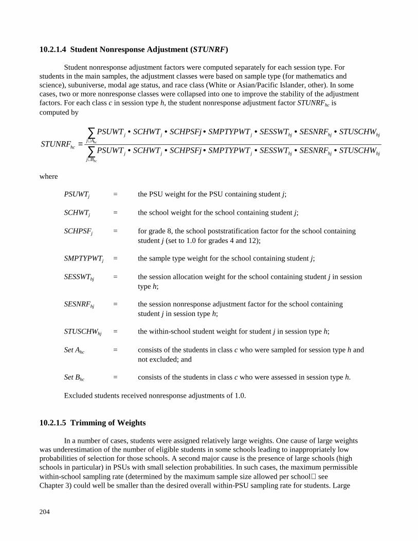
204

10.2.1.4 Student Nonresponse Adjustment (STUNRF)

Student nonresponse adjustment factors were computed separately for each session type. Forstudents in the main samples, the adjustment classes were based on sample type (for mathematics andscience), subuniverse, modal age status, and race class (White or Asian/Pacific Islander, other). In somecases, two or more nonresponse classes were collapsed into one to improve the stability of the adjustmentfactors. For each class c in session type h, the student nonresponse adjustment factor STUNRFhc iscomputed by

∑∑

∈

∈

••••••

••••••=

hc

hc

Bjhjhjhjjjj

Ajhjhjhjjjj

hc STUSCHWSESNRFSESSWTSMPTYPWTSCHPSFjSCHWTPSUWT

STUSCHWSESNRFSESSWTSMPTYPWTSCHPSFjSCHWTPSUWT

STUNRF

where

PSUWTj = the PSU weight for the PSU containing student j;

SCHWTj = the school weight for the school containing student j;

SCHPSFj = for grade 8, the school poststratification factor for the school containingstudent j (set to 1.0 for grades 4 and 12);

SMPTYPWTj = the sample type weight for the school containing student j;

SESSWThj = the session allocation weight for the school containing student j in sessiontype h;

SESNRFhj = the session nonresponse adjustment factor for the school containingstudent j in session type h;

STUSCHWhj = the within-school student weight for student j in session type h;

Set Ahc = consists of the students in class c who were sampled for session type h andnot excluded; and

Set Bhc = consists of the students in class c who were assessed in session type h.

Excluded students received nonresponse adjustments of 1.0.

10.2.1.5 Trimming of Weights

In a number of cases, students were assigned relatively large weights. One cause of large weightswas underestimation of the number of eligible students in some schools leading to inappropriately lowprobabilities of selection for those schools. A second major cause is the presence of large schools (highschools in particular) in PSUs with small selection probabilities. In such cases, the maximum permissiblewithin-school sampling rate (determined by the maximum sample size allowed per school seeChapter 3) could well be smaller than the desired overall within-PSU sampling rate for students. Large

205

weights arose also because very small schools were, by design, sampled with low probabilities. Otherlarge weights arose as the result of high levels of nonresponse coupled with low to moderate probabilitiesof selection, and the compounding of nonresponse adjustments at various levels.

Students with notably large weights have an unusually large impact on estimates such as weightedmeans. Since, under some simplifying assumptions, the variability in weights contributes to the variance ofan overall estimate by an approximate factor 1 + V2, where V2 is the relative variance of the weights, anoccasional unusually large weight is likely to produce large sampling variances of the statistics of interest,especially when the large weights are associated with students with atypical performance characteristics.

To reduce this problem, a procedure of trimming a few of the more extreme weights to valuessomewhat closer to the mean weight was applied. This trimming can increase the accuracy of the resultingsurvey estimates, substantially reducing V2 and hence the sampling variance, while introducing a smallbias. The trimming algorithm was identical to that used since 1984, and had the effect of trimming theweights of students from any school that contributed more than a specified proportion, ζ, to the estimatedvariance of the estimated number of students eligible for assessment. The trimming was done separatelywithin sample type for mathematics and science, and overall for mathematics estimation and mathematicstheme. Trimming was not done for the advanced mathematics or advanced science assessments becauseadvanced students were expected to be concentrated in certain schools, so that the trimming algorithm wasnot appropriate in these cases. In each case, the value of the proportion ζ was chosen to be 10/K, where Kwas the number of schools in which a specified assessment was conducted. The number of schools whereweights were trimmed was no more than seven in any one assessment. The most extreme trimming factorsapplied were of the order of 0.65; trimming affects the weights of only a very small proportion of theassessed and excluded students.

Table 10-2 shows the distributions of eligible students based on the trimmed weights of assessedstudents for the science samples in sample type 2 (the reporting population) for each grade. Thedistributions are similar to those before trimming shown in Tables 10-6, 10-7, and 10-8. To the extent thatthe characteristics in the table are related to student performance on the science assessment, there is asmall bias introduced in the assessment by trimming.

206

Table 10-2Distribution of Populations of Eligible Students Based on Trimmed Weights of Assessed Students

in Participating Schools, 1996 Main NAEP Science Sample, Sample Type 2

Population Grade 4 Grade 8 Grade 12

Total population 3,389,669 3,365,499 2,491,555

Age categoryAt modal age or youngerOlder than modal age

64.6%35.4%

57.9%42.1%

64.5%35.5%

Race/ethnicity categoryWhiteBlackHispanicOther

61.0%14.3%16.9% 7.8%

64.2%15.7%13.6% 6.6%

69.1%12.3%11.1% 7.5%

Gender1

MaleFemale

49.6% 50.2%

50.2%49.6%

48.3%51.7%

SDYesNo

5.2%94.8%

5.7%94.3%

3.1%96.9%

LEPYesNo

3.0%97.0%

1.9%98.1%

2.2%97.8%

SD, LEPSD yes, LEP yesSD yes, LEP noSD no, LEP yesSD no, LEP no

0.1% 5.1% 3.0%

91.8%

0.1% 5.6% 1.8%

92.5%

0.0% 3.0% 2.1%

94.8%1 For a very small percentage of students at grades 4 and 8, gender is unknown.

10.2.1.6 Reporting Factor

Each set of trimmed weights for a given sample type sums to the target population. Reportingfactors were assigned to students in order to scale back the trimmed weights so that final student(reporting) weights within each reporting population (which may combine students from different sampletypes) sum to the target population. The reporting factors assigned to students are specific to the reportingpopulations defined in Table 10-1. Each assessed and excluded student in the reporting populationreceived a reporting factor as shown in Table 10-3 on the following page.

207

Table 10-3Reporting Factors for Assessed and Excluded Students

Non-SD/LEP Students SD/LEP Students———Sample Type——— ———Sample Type———

1 2 3 1 2 3

Grade 4Mathematics 0.5 0.5 — 1 — —Science — 1 — — 1 —Mathematics theme — 1 — — 1 —Mathematics estimation 1 — — 1 — —

Grade 8Mathematics 0.5 0.5 — 1 — —Science — 1 — — 1 —Mathematics theme — 1 — — 1 —Mathematics estimation 1 — — 1 — —Advanced mathematics (B) — 0.35 0.65 — 1 —

Grade 12Mathematics 0.5 0.5 — 1 — —Science — 1 — — 1 —Mathematics theme — 1 — — 1 —Mathematics estimation 0.6667 0.3333 — 1 — —Advanced mathematics (B) — — 1 — — 1Advanced science (C) — 1 — — 1 —

10.2.1.7 Student-Level Poststratification

As in most sample surveys, the respondent weights are random variables that are subject tosampling variability. Even if there were no nonresponse, the respondent weights would at best provideunbiased estimates of the various subgroup proportions. However, since unbiasedness refers to averageperformance over a conceptually infinite number of replications of the sampling, it is unlikely that anygiven estimate, based on the achieved sample, will exactly equal the population value. Furthermore, therespondent weights have been adjusted for nonresponse and a few extreme weights have been reduced insize.

To reduce the mean squared error of estimates using the sampling weights, these weights werefurther adjusted so that estimated population totals for a number of specified subgroups of the population,based on the sum of weights of students of the specified type, were the same as presumably betterestimates based on composites of estimates from the 1993 and 1994 Current Population Survey and 1996population projections made by the U.S. Census Bureau. This adjustment, called poststratification, isintended especially to reduce the mean squared error of estimates relating to student populations that spanseveral subgroups of the population, and thus also to reduce the variance of measures of changes over timefor such student populations.

The poststratification in 1996 was done for the mathematics, science, mathematics estimation, andmathematics theme assessments in each grade. The advanced mathematics and advanced scienceassessments were not poststratified. Within each grade and assessment type group, poststratificationadjustment cells were defined in terms of race, ethnicity, and Census region as shown in Table 10-4. Note

208

that NAEP region was used in previous years instead of Census region. This change was made because thedata from the Current Population Survey and Census Projections are more reliable for Census regions thanfor NAEP regions.

Table 10-4Major Subgroups for Poststratification in 1996

Subgroup Race Ethnicity Census Region1

1234567

WhiteWhiteWhiteWhiteAnyBlackOther

Not HispanicNot HispanicNot HispanicNot HispanicHispanicNot HispanicNot Hispanic

NortheastMidwestSouthWestAnyAnyAny

1 Census region is the same as the NAEP region in Table 3-2 used for stratification andreporting, except that DE, DC, and MD moved from the Northeast to the South, OK andTX moved from the West to the South, Central is called Midwest, and Southeast is calledSouth.

These subgroups were used as adjustment cells at grade 12. Each of these cells accounts forbetween 5 percent (Subgroup 7) and 21 percent (Subgroup 3) of the population. For grades 4 and 8, each ofthe seven subgroups was further divided into two eligibility classes: of modal age and not of modal age.

The procedure used at grade 12 was adopted because the independent estimates of the numbers ofstudents in the population did not provide consistent data on the numbers of twelfth grade students by age.Specifically, the counts of twelfth grade students age 17 and older are not reliable because they includeadult education students. This procedure has been used since 1988. (See Rust, Bethel, Burke, & Hansen,1990, and Rust, Burke, & Fahimi, 1992, for further details.)

Thus, there were 7 or 14 cells for poststratification. The poststratified weight for each studentwithin a particular cell was the student’s base weight, with adjustments for nonresponse and trimming, andthe reporting factor from Section 10.2.1.6, times a poststratification factor. The poststratification factor forstudent j in session type h and poststratification adjustment class c is given by

∑∈

•••••=

hcCjjjjjjBj

chc RPTFCTRTRIMFCTRSTUNRFSCHPSFSESNRFW

TOTALPSFCTR

where

WBj = the base weight for student j (see Section 10.2.1.1);

TOTALc = the total number of grade-eligible students in class c, from the October1993 and 1994 Current Population Surveys and 1996 populationprojections;

SESNRFj = the session nonresponse adjustment factor for the school containingstudent j in session type h;

209

SCHPSFj = for grade 8, the school poststratification factor for the school containingstudent j (set to one for grades 4 and 12);

STUNRFj = the student nonresponse adjustment for student j;

TRIMFCTRj = the trimming factor for student j;

RPTFCTRj = the reporting factor for student j;

Set Chc = consists of the students in class c who were assessed in session type h,except those at grade 12 who were age 17 or older.

Note that students at grade 12 who were age 17 or older received the poststratification factor according totheir adjustment class and session type even though they were not used in calculating the factor. Details ofthe procedures used to obtain totals in the numerator of the adjustment factor are provided in Wallace andRust (1999).

10.2.1.8 The Final Student Reporting Weights

The final weight assigned to a student is the student full-sample reporting weight. This weight isthe student’s base weight after the application of the various adjustments described above. The studentfull-sample reporting weight was used to derive all estimates of population and subpopulationcharacteristics that have been presented in the various NAEP reports, including simple estimates such asthe proportion of students of a specified type who would respond in a certain way to an item and morecomplex estimates such as mean proficiency levels. The distributions of the final student reporting weightsare given in Table 10-5.

As indicated earlier, under some simplifying assumptions the factor 1 + V2 indicates theapproximate relative increase in variance of estimates resulting from the variability in the weights. Thefactor V2 for each sample is readily derivable from Table 10-5 by squaring the ratio of the standarddeviation to the mean weight. These factors, resulting from the combined effect of the variations inweights introduced by design and from other causes, are discussed in Section 10.2.3.

10.2.2 Evaluation of Potential for Bias Resulting from School and Student Nonparticipation

Although school and student nonresponse adjustments are intended to reduce the potential fornonparticipation to bias the assessment results, they cannot completely eliminate this potential bias withcertainty. The extent of bias remains unknown, of course, since there are no assessment data for thenonparticipating schools and students.

Some insight can be gained about the potential for residual nonresponse bias, however, byexamining the weighted school- and student-level distributions of characteristics known for bothparticipants and nonparticipants, especially for those characteristics known or thought likely to be relatedto achievement on the assessment. If the distributions for the full sample of schools (or students) withoutthe use of nonresponse adjustments are close to those for the participants with nonresponse adjustmentsapplied, there is reason to be confident that the bias from nonparticipation is small.

210

Table 10-5Distribution of Final Student Reporting Weights, 1996 Main Samples

SampleNumberof Cases Mean

StandardDeviation Minimum

25thPercentile Median

75thPercentile Maximum

Grade 4 Mathematics 6831 577.41 380.69 92.57 315.28 486.57 729.48 3887.53 Science 8061 489.35 324.35 65.04 275.04 399.02 598.53 4872.34 Mathematics Theme 2072 1903.80 1163.23 576.00 1133.85 1587.94 2276.41 10676.50 Mathematics Estimation 1130 3409.86 2052.49 685.71 1935.01 3010.68 4316.83 12843.05

Grade 8 Mathematics 7312 510.55 389.16 62.92 247.63 389.41 652.26 5027.91 Science 8200 455.26 388.04 75.47 219.81 313.58 562.02 3605.79 Mathematics Theme 2177 1714.81 1124.20 388.72 921.25 1258.58 2321.66 8720.24 Mathematics Estimation 1255 2974.61 1906.19 338.54 1398.58 2574.86 3952.75 9812.97 Advanced Mathematics 2339 346.90 246.57 100.98 184.65 234.99 407.26 1545.58

Grade 12 Mathematics 7020 415.75 257.34 64.39 226.94 337.48 539.29 2313.01

Science 7963 380.19 222.13 64.80 226.82 302.07 500.33 1759.55 Mathematics Theme 2097 1442.96 862.82 313.34 879.14 1117.08 1789.78 5171.06 Mathematics Estimation 1472 1949.24 1050.36 488.10 1170.72 1743.95 2523.71 8484.11 Advanced Mathematics 2972 235.55 127.79 77.16 142.67 182.49 324.65 911.09 Advanced Science 2436 241.49 137.63 58.23 134.85 190.13 323.81 978.81

211

There are several school-level characteristics available for both participating and nonparticipatingschools. The tables below show the combined impact of nonresponse and of the nonresponse adjustmentson the distributions of schools (weighted by the estimated number of eligible students enrolled) andstudents, by the type of school (public, Catholic, other nonpublic) the size of the school as measured by theestimated number of eligible students enrolled, and the urban/rural nature of the place where the school islocated. Three size classes have been defined for each grade. The data are for the science assessment,sample type 2 (the reporting population). Science from sample type 2 was chosen because it is the largestassessment at each grade. It is assumed that other large assessments would behave similarly.

Several student-level characteristics are available for both absent and assessed students. The tablesthat follow show the impact of school nonresponse and nonresponse adjustments, and student nonresponseand nonresponse adjustments on the distributions of eligible students for each grade. This discussion alsofocuses on the science assessment for sample type 2, since it is the largest. The distributions are presentedby age category (at or below modal age, and above modal age), race category (White, Black, Hispanic, andother), gender, SD, and LEP.

Table 10-6 shows the weighted marginal distributions of students for each of the threeclassification variables for each grade, using weighted eligible schools. The distributions before schoolnonresponse adjustments are based on the full sample of in-scope schools for science--those participating,plus those refusals for which no substitute participated. The distributions after school nonresponseadjustments are based only on participating schools for science, with school nonresponse adjustmentsapplied to them.

It can be seen from the tables that, even though the level of school nonparticipation is as high as22.6 percent for grade 12 (see Table 3-11) and somewhat lower for the other grades, for the most part, thedistributions for the three characteristics considered remain similar. Exceptions may be medium and largeschools, and midsize cities and urban fringe of large cities at grade 12; and urban fringe of large cities andrural nonMSAs at grade 4.

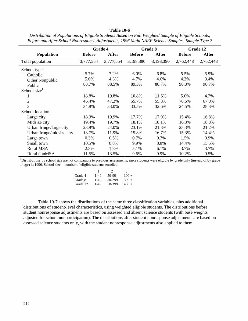
212

Table 10-6Distribution of Populations of Eligible Students Based on Full Weighted Sample of Eligible Schools,

Before and After School Nonresponse Adjustments, 1996 Main NAEP Science Samples, Sample Type 2

Grade 4 Grade 8 Grade 12Population Before After Before After Before After

Total population 3,777,554 3,777,554 3,198,390 3,198,390 2,762,448 2,762,448

School typeCatholicOther NonpublicPublic

5.7% 5.6%88.7%

7.2% 4.3%88.5%

6.0% 4.7%89.3%

6.8% 4.6%88.7%

5.5% 4.2%90.3%

5.9% 3.4%90.7%

School size1

123

18.8%46.4%34.8%

19.8%47.2%33.0%

10.8%55.7%33.5%

11.6%55.8%32.6%

5.0%70.5%24.5%

4.7%67.0%28.3%

School locationLarge cityMidsize cityUrban fringe/large cityUrban fringe/midsize cityLarge townSmall townRural MSARural nonMSA

18.3%19.4%23.9%13.7% 0.3%10.5% 2.3%11.5%

19.9%19.7%24.0%11.9% 0.5% 8.8% 1.8%13.5%

17.7%18.1%23.1%15.8% 0.7% 9.9% 5.1% 9.6%

17.9%18.1%21.8%16.7% 0.7% 8.8% 6.1% 9.9%

15.4%16.3%23.3%15.3% 1.5%14.4% 3.7%10.2%

16.8%18.3%21.2%14.4% 0.9%15.5% 3.7% 9.5%

1 Distributions by school size are not comparable to previous assessments, since students were eligible by grade only (instead of by gradeor age) in 1996. School size = number of eligible students enrolled:

1 2 3Grade 4 1-49 50-99 100 +Grade 8 1-49 50-299 300 +Grade 12 1-49 50-399 400 +

Table 10-7 shows the distributions of the same three classification variables, plus additionaldistributions of student-level characteristics, using weighted eligible students. The distributions beforestudent nonresponse adjustments are based on assessed and absent science students (with base weightsadjusted for school nonparticipation). The distributions after student nonresponse adjustments are based onassessed science students only, with the student nonresponse adjustments also applied to them.

213

Table 10-7Distribution of Populations of Eligible Students Before and After Student Nonresponse Adjustments

1996 Main NAEP Science Samples, Sample Type 2

Grade 4 Grade 8 Grade 12Population Before After Before After Before After

Total population 3,419,493 3,419,493 3,428,867 3,428,867 2,496,241 2,496,241

School typeCatholicOther NonpublicPublic

7.7% 4.5%87.8%

7.8% 4.6%87.6%

6.1% 4.3%89.6%

6.3%4.4%

89.3%

6.4% 3.6%90.0%

8.1% 4.2%87.6%

School locationLarge cityMidsize cityUrban fringe/large cityUrban fringe/midsize cityLarge townSmall townRural MSARural nonMSA

18.9%19.2%25.2%12.1%

0.5%8.9%1.8%

13.3%

18.9%19.3%25.2%12.0%0.5%9.0%1.8%

13.3%

13.2%15.9%20.8%19.3% 0.5%11.6% 7.1%11.6%

13.2%15.9%20.8%19.4% 0.5%11.5% 7.1%11.7%

17.0%18.2%21.4%13.6% 1.0%15.5% 3.9% 9.4%

16.9%16.9%21.7%14.8% 1.0%15.2% 4.1% 9.6%

Age categoryAt modal age or youngerOlder than modal age

64.6%35.4%

64.5%35.5%

57.5%42.5%

57.6%42.4%

64.3%35.7%

64.5%35.5%

Race/ethnicity categoryWhiteBlackHispanicOther

61.4%14.4%16.6% 7.6%

61.2%14.2%16.8% 7.8%

64.9%15.7%13.0% 6.4%

64.7%15.4%13.3% 6.5%

69.4%12.6%11.0% 7.1%

69.1%12.2%11.1% 7.5%

Gender1

MaleFemale

49.6%50.2%

49.6%50.2%

50.3%49.4%

49.6%50.1%

48.7%51.2%

48.4%51.6%

SDYesNo

5.3%94.7%

5.3%94.7%

6.1%93.9%

5.8%94.2%

3.4%96.6%

3.0%97.0%

LEPYesNo

3.0%97.0%

3.0%97.0%

1.9%98.1%

1.9%98.1%

2.1%97.9%

2.2%97.8%

SD, LEPSD yes, LEP yesSD yes, LEP noSD no, LEP yesSD no, LEP no

0.1% 5.2% 2.9%91.8%

0.1% 5.2% 2.9%91.8%

0.1% 6.0% 1.8%92.1%

0.1% 5.7% 1.8%92.5%

0.1% 3.3% 2.1%94.6%

0.0% 3.0% 2.1%94.8%

1 Gender is unknown for a small percentage of students.

The rates of student nonparticipation were 5.1 percent for grade 4, 6.9 percent for grade 8, and22.5 percent for grade 12 (see Table 3-11). The table shows that with one exception at grade 12, for thedistributions of type of school attended and place where the school is located, the combined effect ofstudent nonparticipation and the subsequent nonresponse adjustments have resulted in very little change indistribution. The changes in the distribution of school type at grade 12 reflect the relatively high

214

nonresponse rate of grade 12 public school students (22.7 percent versus 8.5 percent for nonpublic schoolstudents; see Table 3-9).

Table 10-8 shows the weighted distributions of eligible students in participating schools, using thebase weights of assessed and absent students unadjusted for school-level nonresponse. Tables 10-7 and 10-8 show that both school and student-level nonresponse and nonresponse adjustments have little effect onthe distributions of eligible students by age, race/ethnicity, gender, SD and LEP. All of the distributions inthe tables are similar.

Table 10-8Distribution of Populations of Eligible Students Before School and Student Nonresponse Adjustments

1996 Main NAEP Science Samples, Sample Type 2

Population Grade 4 Grade 8 Grade 12

Total population 2,635,218 2,743,713 1,935,174

Age categoryAt modal age or youngerOlder than modal age

64.3%35.7%

56.3%43.7%

63.9%36.1%

Race/ethnicity categoryWhiteBlackHispanicOther

60.8%14.6%16.9% 7.7%

66.6%14.0%13.0%6.5%

70.3%12.4%10.3% 6.9%

Gender1

MaleFemale

49.7%50.1%

50.3%49.5%

48.8%51.2%

SDYesNo

5.3%94.7%

6.2%93.8%

3.4%96.6%

LEPYesNo

3.2%96.8%

2.0%98.8%

2.0%98.0%

SD, LEPSD yes, LEP yesSD yes, LEP noSD no, LEP yesSD no, LEP no

0.1% 5.2% 3.1%91.7%

0.1% 6.1% 1.9%91.9%

0.1% 3.3% 1.9%94.7%

1 Gender is unknown for a small percentage of students.

When comparing the distributions in Table 10-7 before and after student nonresponse adjustments,we expect the distributions by age category and race/ethnicity to be similar because these variables wereused to determine student nonresponse adjustment classes. However, the distributions by gender, SD, andLEP are also similar. To the extent that nonrespondents would perform like respondents with the samecharacteristics (defined by the classification variables in the tables), the bias in the assessment data issmall.

Further information about potential nonresponse bias can be gained by studying the absentstudents. NAEP proficiency estimates are biased to the extent that assessed and absent students within the

215

same weighting class differ in their distribution of proficiency. It seems likely that the assumption thatabsent students are similar in proficiency to assessed students is reasonable for some absentstudents namely, those whose absence can be characterized as random. Conversely, it seems likely thatstudents with longer and more consistent patterns of absenteeism such as truants, dropouts, neardropouts, and the chronically ill are unlikely to be as proficient as their assessed counterparts.

In the 1996 assessments, schools were asked to classify each absent student into one of ninecategories. The results of this classification for the science assessment are shown in Table 10-9. Thediscussion focuses on the science assessment because it is the largest. It is assumed that the other largeassessments would behave similarly.

Table 10-9 shows that, as anticipated, the majority of absence from the assessment was the resultof an absence from school of a temporary and unscheduled nature. The table shows that absence amongtwelfth graders occurs at about four times the rate of absence among fourth or eighth graders. Theproportion of absence classified as temporary differs somewhat by grade, but is of the same magnitude forgrades 8 and 12. These two facts taken together suggest strongly that a substantial proportion of thetemporary absences among twelfth grade students is not a result of illness, because such absences areoccurring at almost three times the rate that they do among fourth or eighth grade students. Whereas itmight be reasonable to regard temporary absence due to illness as independent of proficiency, for othertemporary absences, this appears less tenable. The data in the table give support to the contention that, atgrade 4, student absences are unlikely to introduce any significant bias into NAEP estimates. The absenteerate is low; most absences are temporary, and three quarters of the remaining absences are a result ofparental refusal.

Table 10-9Weighted Distribution of Absent Students by Nature of Absenteeism for All Grades

1996 Science Assessment, Sample Type 2

Nature of Absenteeism Grade 4 Grade 8 Grade 12

Temporary absence1 78.2% 68.0% 63.6%Long-term absence2 1.6% 1.4% 0.8%Chronic truant 0.2% 2.7% 1.4%Suspended or expelled 0.7% 6.4% 0.4%Parent refusal 16.4% 13.1% 9.2%Student refusal 0.0% 3.2% 12.0%In school, did not attend session 0.0% 3.0% 7.0%In school, not invited3 0.0% 0.8% 0.0%Other 0.3% 0.9% 3.9%Missing 2.6% 0.4% 1.8%Total absentee sample 384 569 2,269Total sample size 7,689 8,343 9,807Overall absentee rate 5.0% 6.8% 23.1%

1 Absent less than two weeks due to illness, disability, or excused absence.2 Absent more than two weeks due to illness or disability.3 In school, but not invited to assessment session due to disruptive behavior.

At grades 8 and 12, however, a significant component of absenteeism is not temporary or due toparental refusal. Chronic truants, those suspended, and those in school but not invited, constitute theobvious candidates for potential bias. These groups comprise 12.1 percent of absent students at grade 8 (or

216

0.8 percent of the total sample) and 8.8 percent of absent students at grade 12 (or 2.0 percent of the totalsample). Thus their potential for introducing significant bias under the current procedures is minor.

10.2.3 Derivation of Modular Weights for the Main Samples

As discussed earlier, modular weights were computed to facilitate analyses involving studentsfrom a single sample type. The same procedures were used to derive modular and reporting weights upthrough the weight trimming step described in Section 10.2.1.5. After trimming, weighting continued intwo parallel processes. Final student reporting weights were the result of one of these processes, andmodular weights were the result of the other.

Modular weights differ from reporting weights in two ways. First, they do not contain thereporting factor described in Section 10.2.1.6. The second difference lies in the manner in which theweights were poststratified. The modular weights were poststratified as described in Section 10.2.1.7,except that each sample type within each grade and session was poststratified separately. The same initialadjustment cells were used: 7 cells based on race/region for each session/sample type combination at grade12, and 14 cells based on race/region and eligibility class (of modal age, not of modal age) for eachsession/ sample type combination at grades 4 and 8. Some adjustment factors are quite variable for thesame adjustment cell across different sample types for the same grade and session. This indicates that theindividual samples by sample type may not be particularly stable, especially for the smaller sessions ofmathematics theme and mathematics estimation.

The modular weight is the student’s base weight after the application of the various adjustmentsdescribed in Section 10.2.1, except for the reporting factor, and with the new poststratification factordescribed above. The distributions of the modular weights are given in Table 10-10. Note that modularweights are identical to reporting weights for a particular grade/session/sample type combination when thatsample type is the only one included in the reporting population for that grade and session.

10.2.4 Derivation of Student Weights for the Long-Term Trend Samples

Final student weights were derived for the long-term trend samples in a manner similar to that usedin 1994. The procedure was identical to that used to derive reporting weights, described in Section 10.2.1,except as noted below.

As in 1994, excluded students for all subjects in the long-term trend samples were weightedtogether, separately from assessed students.

Base weight. A student’s base weight is the reciprocal of the product of four factors all of thefactors used for reporting weights except sample type weight (SMPTYPWT).

Session nonresponse adjustments. Session nonresponse adjustments were calculated separately ateach age class for the spiral assessment, the tape assessment, and excluded students, within classes formedby subuniverse. The formula for the adjustment does not contain sample type weight (SMPTYPWT), andfor excluded students, it does not contain session allocation weight (SESSWT). Gi is the estimated numberof age- plus grade-eligible students in the school for the spiral assessment and excluded students, and theestimated number of age-eligible students for the tape assessment. For excluded students, Sets B and C arenot specific to any particular session.

217

Table 10-10Distribution of Modular Weights, Main Samples

Grade/Session/Sample Type

Number ofCases Mean

StandardDeviation Minimum

25thPercentile Median

75thPercentile Maximum

Grade 4Mathematics/1 3808 1035.39 615.46 163.33 579.23 903.43 1366.37 3812.67Mathematics/2 3691 1068.73 626.06 207.26 637.04 930.71 1305.99 4446.43Mathematics/3 4077 967.54 670.28 211.91 513.62 759.53 1208.03 6569.06Science/2 8061 489.35 324.35 65.04 275.04 399.02 598.53 4872.34Science/3 4600 857.54 591.01 108.77 463.61 646.17 1032.26 4642.09Mathematics Theme/2 2072 1903.80 1163.23 576.00 1133.85 1587.94 2276.80 10676.50Mathematics Theme/3 2239 1761.80 1061.66 178.33 1063.45 1373.85 2247.80 9972.62Mathematics Estimation/1 1130 3490.86 2052.49 685.71 1935.45 3010.68 4316.83 12843.05Mathematics Estimation/3 1109 3556.97 2235.80 1006.89 2080.57 2916.57 4161.25 13829.45

Grade 8Mathematics/1 4107 908.97 620.95 106.84 405.18 770.50 1241.29 4313.67Mathematics/2 4004 932.35 802.10 146.84 465.54 637.59 1098.33 6675.87Mathematics/3 4128 904.35 571.76 165.42 505.73 704.53 1175.81 5003.16Science/2 8200 455.26 388.04 75.47 219.81 313.58 562.02 3605.79Science/3 4520 825.92 634.43 113.78 386.38 611.60 1026.86 4287.45Mathematics Theme/2 2177 1714.81 1124.20 388.72 921.25 1258.58 2321.66 8720.24Mathematics Theme/3 2264 1648.91 1050.29 459.90 889.19 1384.34 2006.79 6131.34Mathematics Estimation/1 1255 2974.61 1906.19 338.54 1398.58 2574.86 3952.75 9812.97Mathematics Estimation/3 1097 3403.04 1856.24 663.36 1873.01 3079.88 4303.41 13067.90Advanced Mathematics/2 805 890.46 661.32 288.53 511.84 645.93 891.71 3849.92Advanced Mathematics/3 1562 557.79 386.61 185.10 286.90 385.01 684.21 2377.82

Grade 12Mathematics/1 3732 789.88 495.08 119.49 415.49 600.65 1100.18 3508.86Mathematics/2 3913 750.91 451.42 103.41 434.29 614.34 1036.98 4104.76Mathematics/3 3672 828.88 521.21 65.20 467.94 683.04 1071.83 2884.61Science/2 7963 380.19 222.13 64.80 226.82 302.07 500.33 1759.55Science/3 4179 718.80 465.56 66.96 406.63 587.94 884.80 3559.46Mathematics Theme/2 2097 1442.96 862.82 313.34 879.14 1117.08 1789.78 5171.06Mathematics Theme/3 1944 1524.34 789.35 434.13 922.15 1248.22 1991.56 6331.79Mathematics Estimation/1 1090 2616.75 1353.39 667.28 1641.53 2331.77 3387.79 7581.54Mathematics Estimation/2 431 6810.82 3947.11 2181.87 4076.82 5516.38 8886.82 19094.18Mathematics Estimation/3 458 6384.23 4477.96 2416.15 3611.22 4792.51 6366.71 23079.02Advanced Mathematics/3 2972 235.55 127.79 77.16 142.67 182.49 324.65 911.09Advanced Science/2 2436 241.49 137.63 58.23 134.85 190.13 323.81 978.81

218

School-level poststratification. There was no school-level poststratification for the long-term trendassessments.

Student nonresponse adjustments. Student nonresponse adjustments were calculated separately ateach age class for the spiral assessment and the tape assessment within classes formed by subuniverse andmodal grade status (at or above modal grade, below modal grade). For excluded students at each age class,the adjustments were calculated within classes formed by subuniverse. The formula for the adjustment doesnot contain sample type weight (SMPTYPWT) or the school-level poststratification factor (SCHPSF), and forexcluded students, it does not contain session allocation weight (SESSWT). For excluded students, Set Aconsists of all excluded students in class C, and Set B consists of the excluded students in class C for whoman excluded student questionnaire was completed.

Trimming. Trimming was done separately for the spiral assessment, the tape assessment, andexcluded students at each age class.

Reporting factor: There was no reporting factor for the long-term trend assessments.

Student-level poststratification. Poststratification adjustments were calculated separately at eachage class for the spiral assessment, the tape assessment, and excluded students. Adjustment cells wereformed by race/region (as described in Section 10.2.1.7) and eligibility class (eligible by grade and of modalage, eligible by age only, and eligible by grade but not of modal age). Thus 21 cells were used for the spiralassessment and excluded students at each age class. Seven cells (by race/region only) were used for the tapeassessment at each age class. For each cell the poststratification factor is a ratio whose denominator is thesum of weights (after adjustments for nonresponse and trimming) of assessed and excluded students, andwhose numerator is an adjusted estimate of the total number of students in the population who are membersof the cell.

Final student weights. The final weight assigned to each student is the student’s base weight afterapplication of the various adjustments described above. The distributions of the final student weights for thelong-term trend samples are given in Table 10-11.

10.2.5 Other Weights

Special weighting adjustments were developed for certain subsets of the fourth-grade and eighth-grade students assessed in the main samples. The weights for these subsets, with these adjustments applied,were used in equating the results of the national and state assessments for subjects they had in common.Also, weights appropriate for analyzing school-level data files were developed.

10.2.5.1 Weights for Equating National and State-by-State Samples

Weights for Equating National and State-by-State Assessments. The fourth-grade mathematics andeighth-grade mathematics and science assessments conducted in February 1996 in the NAEP 1996 StateAssessment consisted of identical assessment material to that administered in the corresponding nationalmain sample sessions. Technical details of the NAEP 1996 State Assessments are given in Allen, Jenkins,Kulick, and Zelenak (1997) and Allen, Swinton, Isham, and Zelenak (1998). The national and state-by-stateassessments were equated so that state and national results could be reported on a common scale. Theequating was achieved by using from each assessment that part of the sample representing a commonpopulation. For the national samples, this consisted of those fourth-grade or eighth-grade public-school

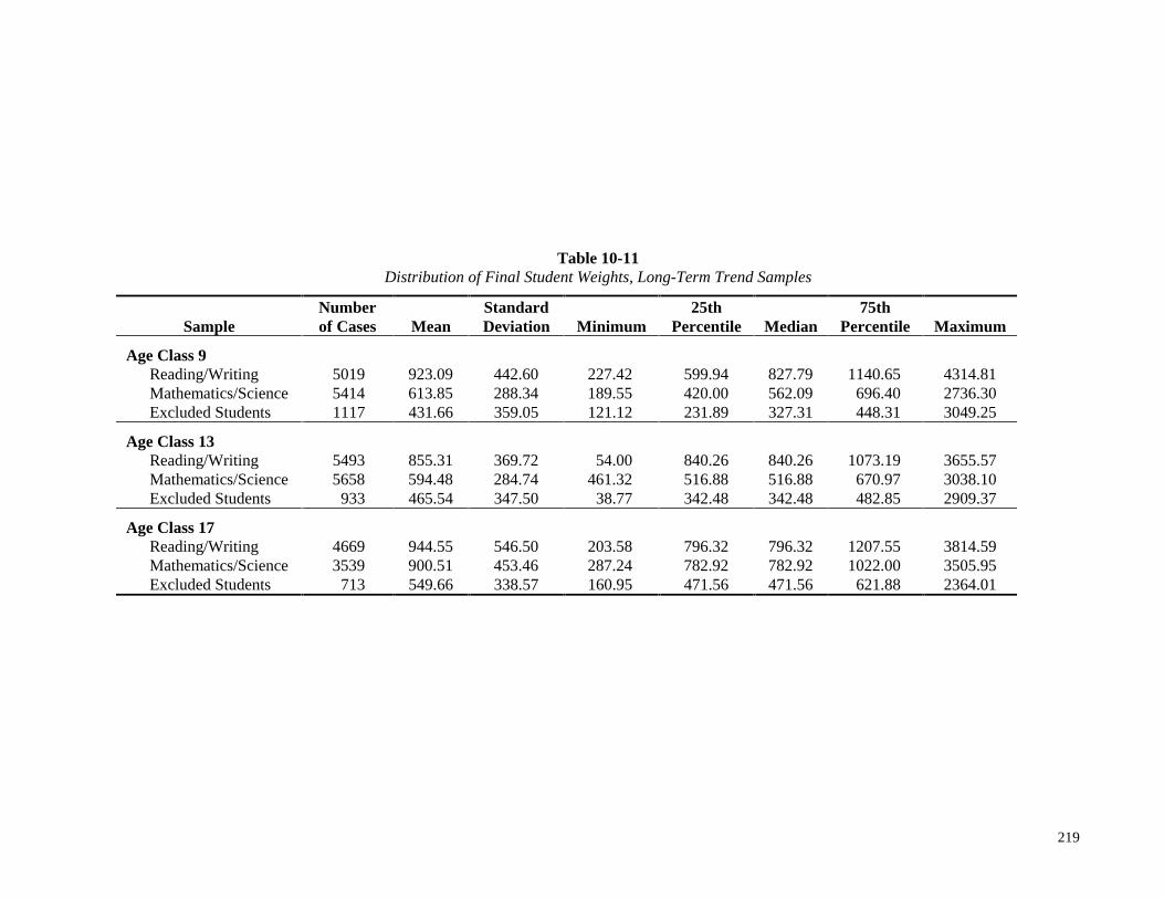
219

Table 10-11Distribution of Final Student Weights, Long-Term Trend Samples

SampleNumberof Cases Mean

StandardDeviation Minimum

25thPercentile Median

75thPercentile Maximum

Age Class 9Reading/Writing 5019 923.09 442.60 227.42 599.94 827.79 1140.65 4314.81Mathematics/Science 5414 613.85 288.34 189.55 420.00 562.09 696.40 2736.30Excluded Students 1117 431.66 359.05 121.12 231.89 327.31 448.31 3049.25

Age Class 13Reading/Writing 5493 855.31 369.72 54.00 840.26 840.26 1073.19 3655.57Mathematics/Science 5658 594.48 284.74 461.32 516.88 516.88 670.97 3038.10Excluded Students 933 465.54 347.50 38.77 342.48 342.48 482.85 2909.37

Age Class 17Reading/Writing 4669 944.55 546.50 203.58 796.32 796.32 1207.55 3814.59Mathematics/Science 3539 900.51 453.46 287.24 782.92 782.92 1022.00 3505.95Excluded Students 713 549.66 338.57 160.95 471.56 471.56 621.88 2364.01

220

students from a participating state (including the District of Columbia) who were assessed in the mainsample mathematics or (for grade 8) science assessment reporting samples.

Although each sample of students received appropriate weights from the weighting procedure usedfor the national assessment, in an effort to increase the precision of the equating process, an additionalweighting adjustment was developed and applied to each subsample by grade and subject, solely for use inequating. For each subsample, the distributions of the main sample reporting weights for three categoricalvariables were adjusted to agree closely with those obtained from the weighted aggregate sample from thestate assessments from the participating states. The first two variables were NAEP region (Northeast,Southeast, Central, and West) and race/ethnicity (White nonHispanic, Black nonHispanic, Hispanic, andother). For fourth-grade mathematics, the third variable was mathematics skill (good, not sure, other). Foreighth-grade mathematics, the third variable was the student’s mathematics course (eighth-grademathematics, pre-algebra, algebra, other). For eighth-grade science, the third variable was the student’sscience course (earth science only, physical science only or only earth science and physical science, other).The categorical variables and control totals for each of the assessed grades and subjects are presented inTables 10-12 and 10-13.

Table 10-12First and Second Categorical Variables Used for Raking1

RakingDimensions

Fourth Grade MathematicsControl Total

Eighth Grade MathematicsControl Total

Eighth Grade ScienceControl Total

First DimensionNAEP Region

1. Northeast 631,451 480,785 475,0792. Southeast 733,191 723,032 726,3223. Central 427,577 433,541 432,5804. West 932,339 904,369 915,815Total 2,724,558 2,541,727 2,549,797

Second DimensionRace/Ethnicity

1. White nonHispanic 1,690,310 1,596,274 1,590,1642. Black nonHispanic 408,725 377,660 372,7153. Hispanic 454,883 408,197 419,4674. Other 170,641 159,595 167,451Total 2,724,558 2,541,727 2,549,797

1 Numbers may not add up exactly due to rounding.

The equating of each weight distribution was achieved using a procedure known as iterativeproportional fitting (described by Little & Rubin, 1987). At the end of the fitting, adjustment factors werederived and multiplied to the main sample weights for each subgroup to force their distribution to agreewith that from the aggregated state samples, for each of these three variables in turn. This process was thenrepeated, and the final set of adjusted weights was compared with the state sample weights on all threedistributions, and found to be in very close agreement. Table 10-14 shows the distribution of theadjustment factors for each of the grades and subjects assessed.

221

Table 10-13Third Categorical Variable Used for Raking1

Control Totals

Grade 4Mathematics Skill

1. Good 1,734,0932. Not sure 634,7323. Other 355,733Total 2,724,558

Grade 8Mathematics Type Course

1. Eight Grade Mathematics 1,018,7432. Pre-Algebra 714,9253. Algebra 639,3934. Other 168,665Total 2,541,727

Science Type Course1. Earth Sciences only 737,8982. Physical Sciences only or Earth Science and Physical Science 525,0483. Other 1,286,851Total 2,549,797

1 Numbers may not add up exactly due to rounding.

Table 10-14Percentiles of Raking Adjustments

Distribution Grade 4 Mathematics Grade 8 Mathematics Grade 8 Science

Minimum 0.587 0.708 0.72110th Percentile 0.699 0.741 0.81025th Percentile 0.777 0.837 0.847Median 0.891 0.958 0.98375th Percentile 1.025 1.074 1.16190th Percentile 1.119 1.230 1.409Maximum 1.524 1.728 2.355

10.2.5.2 School Weights

The sampling procedures used to obtain national probability samples of assessed students alsogave rise indirectly to several national probability samples of schools (from which the students weresubsequently sampled). So that the school samples can be utilized for making national estimates aboutschools, appropriate nonresponse adjusted survey weights have been developed.

For the first time in 1996, the school weights for the main assessments were computed separatelyby subject within grade. The school weights were a direct byproduct of the student weighting process. Theweight for school i in session h is given by

Whi = PSUWTi • SCHWTi • SESSWThi • SESNRFhi • SCHPSFhi

222

where PSUWTi, SCHWTi, SESSWThi, SESNRFhi, and SCHPSFhi are defined in Section 10.2.1.

The school weights for the long-term trend assessments in 1996 were computed using the sameprocedures used in earlier years. The weights were computed separately by age class. The school baseweight was the product of PSUWT and SCHWT. School nonresponse adjustments were then applied tothese base weights. The values of the adjustment factors are not subject specific. In fact, they are identicalto the school nonresponse adjustment factors used for excluded students. Schools that did not participate inany of the sessions that they were assigned were treated as nonrespondents, but schools that conducted atleast one of their assigned sessions were treated as respondents.

Fifteen samples of schools were weighted to be nationally representative in the main assessments,and three samples were weighted to be nationally representative in the long-term trend assessments. In themain samples, the population of schools represented is that of schools with grade 4 (for the grade 4assessments), grade 8 (for the grade 8 assessments), or grade 12 (for the grade 12 assessments). In thelong-term trend samples, the school population at age class 9 is that of schools having eligible students andat least one of the grades 2 through 5, the school population at age class 13 is that of schools havingeligible students and at least one of the grades 6 through 9, while the school population at age class 17 isthat of schools having eligible students and at least one of the grades 9 through 12.

10.2.5.3 Jackknife Replicate Weights

In addition to the weights that were used to derive all estimates of population and subpopulationcharacteristics, other sets of weights, called jackknife replicate weights, were derived to facilitate theestimation of sampling variability by the jackknife variance estimation technique. These weights and thejackknife estimator are discussed in the next section.

10.3 PROCEDURES USED BY NAEP TO ESTIMATE SAMPLING VARIABILITY

A major source of uncertainty in the estimation of the value in the population of a variable ofinterest exists because information about the variable is obtained on only a sample from the population. Toreflect this fact, it is important to attach to any statistic (e.g., a mean) an estimate of the samplingvariability to be expected for that statistic. Estimates of sampling variability provide information abouthow much the value of a given statistic would be likely to change if the statistic had been based on another,equivalent, sample of individuals drawn in exactly the same manner as the achieved sample.

Another important source of variability is that due to imprecision in the measurement of individualproficiencies. For the 1996 assessment, proficiencies in all subject areas were summarized through itemresponse theory (IRT) models, but not in the way that these models are used in standard applications whereeach person responds to enough items to allow for precise estimation of that person’s proficiency. InNAEP, each individual responds to relatively few items so that individual proficiency values are not welldetermined. Consequently, the variance of any statistic based on proficiency values has a component dueto the imprecision in the measurement of the proficiencies of the sampled individuals in addition to acomponent measuring sampling variability. The estimation of the component of variability due tomeasurement imprecision and its effect on the total variability of statistics based on proficiency values arediscussed in Chapter 11.

223

The estimation of the sampling variability of any statistic must take into account the sampledesign. In particular, because of the effects of cluster selection (students within schools, schools withinPSUs) and because of effects of nonresponse and poststratification adjustments, observations made ondifferent students cannot be assumed to be independent of each other (and are, in fact, generally positivelycorrelated). Furthermore, to account for the differential probabilities of selection (and the variousadjustments), each student has an associated sampling weight, which should be used in the computation ofany statistic and which is itself subject to sampling variability. Ignoring the special characteristics of thesample design and treating the data as if the observations were independent and identically distributed, willgenerally produce underestimates of the true sampling variability, due to the clustering and unequalsampling weights.

The proper estimation of the sampling variability of a statistic based on the NAEP data iscomplicated and requires techniques beyond those commonly available in standard statistical packages.Fortunately, the jackknife procedure (see, e.g., Wolter, 1985; Kish & Frankel, 1974; Rust, 1985) providesgood quality estimates of the sampling variability of most statistics, at the expense of increasedcomputation, and can be used in concert with standard statistical packages to obtain a proper estimate ofsampling variability.

The jackknife procedure used by NAEP has a number of properties that make it particularly suitedfor the analysis of NAEP data. When properly applied, a jackknife estimate of the variability of a linearestimator (such as a total) will be the same as the standard textbook variance estimate specified for thesample design (if the first-stage units were sampled with replacement and approximately so otherwise).Additionally, if the finite sampling corrections for the first stage units can be ignored, the jackknifeproduces asymptotically consistent variance estimates for statistics such as ratios, regression estimates orweighted means and for any other nonlinear statistic that can be expressed as a smooth function ofestimated totals of one or more variables (Krewski & Rao, 1981).

Through the creation of student replicate weights (defined below), the jackknife procedure allowsthe measurement of variability attributable to the use of poststratification and other weight adjustmentfactors that are dependent upon the observed sample data. Once these replicate weights are derived, it is astraightforward matter to obtain the jackknife variance estimate of any statistic.

The jackknife procedure in this application is based upon the development of a set of jackknifereplicate weights for each assessed student (or excluded student, or school depending upon the fileinvolved). The replicate weights are developed in such a way that, when utilized as described below,approximately unbiased estimates of the sampling variance of an estimate result, with an adequate numberof degrees of freedom to be useful for purposes of making inferences about the parameter of interest.

The estimated sampling variance of a parameter estimator t is the sum of M squared differences(where M is the number of replicate weights developed):

�Var t t ti

i

M

� � � �= −=∑

1

2,

where ti denotes the estimator of the parameter of interest, obtained using the ith set of replicate weights,SRWTi, in place of the original sample of full sample estimates WT.

For each of the three sample types (see Section 3.4 and Chapter 5 for a description of the threesample types) in the main assessment samples, 62 replicate weights were developed using the proceduresoutlined below. Similar procedures were followed for the long term trend samples. However, since those

224

samples were based on fewer PSUs (52 rather than 94), the long-term trend samples have fewer replicateweights (36 instead of 62). Full details of the generation of replicate weights for all samples are given inWallace and Rust (1999).

Of the 62 replicate weights formed for each record from a main assessment sample, 36 act toreflect the amount of sampling variance contributed by the noncertainty strata of PSUs, with the remaining26 replicate weights reflecting the variance contribution of the certainty PSU samples.

The derivation of the 36 replicate weights reflecting the variance of the noncertainty PSUsinvolves first defining pairs of PSUs in a manner that models the design as one in which two PSUs aredrawn with replacement per stratum. This definition of pairs is undertaken in a manner closely reflective ofthe actual design, in that PSUs are pairs that are drawn from strata within the same subuniverse, and withsimilar stratum characteristics. The same definition of pairs was used for each of the age/grade classes inthe main assessment, since all were drawn from the same sample of noncertainty PSUs. The 72noncertainty PSUs, drawn one from each of 72 strata, were formed into 36 pairs of PSUs, where the pairswere composed of PSUs from adjacent strata within each subuniverse (thus the strata were relativelysimilar on socioeconomic characteristics such as proportion minority population, population change since1980, per capita income, educational attainment, and unemployment rate). Whereas the actual sampledesign was to select one PSU with probability proportional to size from each of 72 strata, for varianceestimation purposes the design is regarded as calling for the selection of two PSUs with probabilityproportional to size with replacement from each of 36 strata. This procedure likely gives a small positivebias to estimates of sampling error.

The student replicate weight for the ith pair of noncertainty PSUs, for the 36 pairs corresponding tovalues of i from 1 to 36, is computed as follows:

1. Let WB be the base weight of a student, as described in Section 10.2.1, which accountsfor the various components of the selection probability for the student.

2. At random, one PSU in each pair is denoted as PSU number 1, while the other is

denoted as PSU number 2. The ith replicate base weight Wbi is given by:

W

i

W i

WB i

bi B=�����

0

2

if the student belongs to PSU number 1 of pair

if the student belongs to PSU number 2 of pair

if the student is from neither PSU in pair

*

3. The ith student replicate weight SRWTi is obtained by applying the various school andstudent nonresponse adjustments, the weight trimming, and the poststratification to theith set of replicate base weights, using procedures identical to those used to obtain thefinal student weights WT from the set of base weights WB.

In brief, the procedure for deriving the sets of Wbi values from the WB values reflects the samplingof PSUs, schools, sessions, and students. By repeating the various weight adjustment procedures in eachset of replicate base weights, the impact of these procedures on the sampling variance of the estimator, t, isappropriately reflected in the variance estimator Var t� � � defined above.

The procedure for obtaining the 26 sets of replicate weights to estimate the sampling variance fromthe certainty PSUs is analogous, but somewhat more complex. The first stage of sampling in this case is atthe school level, and the derivation of replicate weights must reflect appropriately the sampling of schoolswithin certainty PSUs. Since each of the three grade classes in the main assessment involved different

225

samples of schools, the procedure for forming replicate base weights was individualized to each of thesesample components. In common across these three samples were the 22 certainty PSUs used, and the factthat 26 replicate weights were formed in each case.

For a given sample, the 22 certainty PSUs constituted strata, with a sample of schools drawnsystematically within each. Using the schools listed in order of sample selection within each stratum,successive schools were paired or formed into triples. These pairs and triples numbered more than 26, sothat each replicate weight was in general formed by perturbing the weights of students from more than asingle pair or triple. These aggregates of pairs and triples were in general assigned in proportion to the sizeof the PSU. Thus generally speaking, the largest PSUs were assigned three replicates each, the next largestwere assigned two replicates each, and the remaining self-representing PSUs were assigned one replicateeach. When splitting the larger PSUs, the schools were split into groups of (as close as possible) equal size,based on the ordering at the time of sample selection. One group was assigned to each replicate. Withineach PSU (or partial PSU in the case of the large split PSUs) schools were alternately numbered 1 or 2starting randomly. If, however, there were exactly three schools sampled in the PSU the schools wererandomly numbered 1, 2, or 3. The method of forming replicate base weights in strata where there were notexactly three schools was the same as for the noncertainty strata (except that members of a pair, i, couldcome from more than a single “stratum”).

When a stratum contained three schools, students in these schools had their weights perturbed fortwo sets of replicates, say i1 and i2, as follows:

W

i

W i

W i

bi B

B

=�����

0

1 5

if the student is in school number 1 of a PSU belonging to set

if the student is in school number 2 or 3 of a PSU belonging to set

if the student does not belong to a PSU in set

. *

W

W i

i

W i

bi

B

B

=�����

1 5

0

. * if the student is in school number 1 or 2 of a PSU belonging to set

if the student is in school number 3 of a PSU belonging to set

if the student does not belong to a PSU in set

The actual pattern of replicate base weight assignment used for each of the samples is given inWallace and Rust (1999).

The nonresponse, trimming, and poststratification adjustments were applied to each set of replicatebase weights to derive the final replicate weights in each case, exactly as in the noncertainty PSUs. In factthese procedures were applied to the full set of weights from all parts of the given sample together, just asfor the full sample weights. That is, for example, poststratification factors were derived from the full set ofdata for each replicate, not separately for certainty and noncertainty PSUs.

This estimation technique was used by NAEP to estimate all sampling errors presented in thevarious reports. A further discussion of the variance estimation procedure used by NAEP, including adiscussion of alternative jackknife estimators that were also considered, appears in Johnson (1989).

We noted above (as discussed in Chapter 11) that a separate estimate of the contribution tovariance due to the imprecision in the measure of individual proficiencies is made and added to thejackknife estimate of variance. That variance component could have been approximately reflected in thejackknife variance estimates simply by separately applying the IRT computations to each jackknifereplicate. Because of the heavier IRT computational load, this was not done. Less work was involved bythe simple procedure of making separate estimates of this component to be added to the jackknife variance

226

estimates. Also, a separate measure of this component of variance is then available, which would not be soif it were reflected in the jackknife variance estimate.

10.4 APPROXIMATING THE SAMPLING VARIANCE USING DESIGN EFFECTS

In practical terms, the major expenditure of resources in the computation of a jackknife varianceestimate occurs in the preparation of estimates for each of the pseudoreplicates. In the 1996 assessment,this implies that the statistic of interest has to be recomputed up to 63 times, once for the overall estimate t,and once for each of the up to 62 pseudoreplicates ti. Because this is a considerable increase in the amountof computation required, relative to a conventional variance estimate, it is of interest to see how much thejackknife variance estimates differ from their less computationally intensive, simple random samplingbased, analogues.

The comparison of the conventional and the jackknife methods of variance estimation will be interms of a statistic called the design effect, which was developed by Kish (1965) and extended by Kish andFrankel (1974). The design effect for a statistic is the ratio of the actual variance of the statistic (taking thesample design into account) over the conventional variance estimate based on a simple random samplewith the same number of elements. The design effect is the inflation factor to be applied to theconventional variance estimate in order to adjust error estimates based on simple random samplingassumptions to account approximately for the effect of the sample design. The value of the design effectdepends on the type of statistic computed and the variables considered in a particular analysis as well asthe combined clustering, stratification, and weighting effects occurring among sampled elements. Whilestratification drives down the sampling variance, the effects of clustering and weighting that drivevariances up are generally sufficient to produce variance estimates that are larger than variances based onsimple random sampling assumptions. Consequently, the design effects will be greater than one. In NAEP,the underestimates are the result of ignoring the effects of clustering and unequal probabilities of selectionin the variance calculations.

Since most of the analyses conducted by NAEP are based on the results of scaling models thatsummarize performance of students across a learning area, we consider the design effects to be expectedfor analyses based on these scale scores. For reasons given in Chapter 11, NAEP provides each individualwith a set of “plausible values,” each of which is a random draw from the distribution of the potential scalescores for that individual. Since our current interest is on the effect of the sampling design on estimationand inference, we will restrict our attention to a single measure of an individual’s proficiency, the firstplausible value of the individual’s scale score.

A key statistic of interest is the estimated mean proficiency of a subgroup of the population. Anestimate of the subgroup mean proficiency is the weighted mean of the first plausible values of proficiency

of the sampled individuals who belong to the subpopulation of interest. Let Y be the weighted mean of theplausible values of the sampled members of the subpopulation. The conventional estimate of the variance

of Y is

Var Yw y Y

N Wcon

i i

i

N

� �� �

=−

=

+

∑ 2

1 ,

where N is the total number of sampled individuals in the subpopulation for which plausible values areavailable, wi is the weight of the ith individual, yi is a plausible value from the distribution of potentialproficiencies for that individual, and W+ is the sum of the weights across the N individuals.

227

The design effect for the subgroup mean proficiency estimate is

deff Y Var Y Var YJK con� � � � � �= /

where VARJK(Y ) is the jackknife variance of Y . (As has been pointed out previously, VARJK(Y ) ascomputed does not measure the variability of Y due to imprecision in the measurement of the proficienciesof the sampled individuals. The estimation of this very important source of variability is discussed inChapter 11.) Of the factors that determine deff(Y ), the effects of stratification are usually less than one,which means the efficiency of a stratified sampling is better than a simple random sampling; whereas theclustering effects are always larger than one. The clustering effects can be approximated by

1 1+ −m� �ρ ,

where m is the average cluster size and ρ is the intracluster correlation (Cochran, 1977). Therefore, thelarge cluster size or large intracluster correlation will inflate the clustering effects.

Values of the design effects for subgroup mean proficiencies are displayed, by grade, in Tables 10-15 and 10-19 for the 1996 main assessments of mathematics and science respectively. Design effects areshown for the population as a whole (Total) as well as for a variety of demographic subgroups: gender;race/ethnicity (White, Black, Hispanic, Asian/Pacific Islander, other); type of location (Central City, UrbanFringe/Large Town, Rural/Small Town); parental education (did not graduate high school, graduated highschool, post-high school, graduated college, unknown); and type of school (public, nonpublic). Theseparticular demographic variables were selected because (1) they are major variables in NAEP reports and(2) they reflect different types of divisions of the population that might have different levels of samplingvariability. Note that the tables of the design effects provided in the NAEP Technical Reports previous to1994 are computed for the mean item scores, proportion-correct statistics, which can not be compared withthe design effects for proficiency scale scores directly.

The 1996 main mathematics assessment contains the three sample types S1, S2 and S3 (seeSection 5.3). To conserve trend in the main mathematics assessment, the reporting samples were made upof A1 and B1 portions in S1 samples and A2 in S2 samples (see Table 10-1). The advantage of includingA2 in the reporting samples is to obtain more accurate scale scores, yet a trade-off is that the clusteringeffects for the reporting samples becomes lager than the clustering effects for only sample S1.

The larger intracluster correlation in A1 and A2 and larger cluster sizes in sample type S1 are twofactors that contribute to the increase in clustering effects. First, the reporting sample for the mainmathematics assessment from sample type S2 has only non-SD/LEP students, A2. Compared with theSD/LEP students, the non-SD/LEP students are relative homogenous in scale scores. The highhomogeneity in clusters implies a large intracluster correlation, ρ1. Given other conditions, the largeclustering effects that are due to a large intracluster correlation expand the design effects in the reportingsamples. To check this conclusion, the design effects for subsamples of A1, A2, and B1 were calculatedseparately and are displayed in Tables 10-16, 10-17 and 10-18. The estimated design effects forsubsamples of A1 and A2 are much larger than those for subsample B1 that contains SD/LEP students insample type S1. Secondly, the cluster sizes tended to be larger in sample type S1 because the schools insample type S1 only provided samples for the main mathematics assessment, whereas the schools insample type S2 provided samples for both the main mathematics and science assessments. Therefore, thedesign effects in A1 are found to be larger than the design effects in A2 and both subsamples of A1 and A2contributed students to the reporting samples.

228

Tables 10-20 and 10-21 provide equivalent information for the long-term trend samples. Table 10-20provides, for each age class and demographic subgroup, the average of the design effects for mean readingand writing proficiencies for the students selected for the long-term trend assessments of reading andwriting. Table 10-21 provides the average of the design effects for the mean mathematics and scienceproficiencies for the students selected for the long-term trend assessments of mathematics and science.

Finally, for comparison with the national mathematics and science results, Table 10-22 shows theaverage design effects for state-level mean mathematics proficiency, averaged across all jurisdictionsparticipating in the grade 4 and grade 8 1996 State Assessment in mathematics. The results in Table 10-23are the average design effects for state-level mean science proficiency, averaged across all jurisdictionsparticipating in the grade 8 1996 State Assessment in science.

The tables show that the design effects are predominantly larger than 1, indicating that standard varianceestimation formulas will be generally too small, usually markedly so. Although the design effects appearsomewhat different for certain subgroups of the population, they are, perhaps, similar enough (at least withina subject and grade) to select an overall composite value that is adequate for most purposes. In choosing acomposite design effect, some consideration must be made about the relative consequences ofoverestimating the variance as opposed to underestimating the variance. For example, if an overestimate ofthe variance is viewed as severe an error as an underestimate, the composite design effect should be near tothe center of the distributions of the design effects. Possible composites of this type are the mean andmedian design effects across the combined distribution of all design effects. Larger design effects should beused if it is felt that it is a graver error to underestimate the variability of a statistic than to overestimate it.For example, Johnson and King (1987) examine estimation of variances using design effects (among othertechniques) under the assumption that the consequences of an underestimate are three times as severe asthose of an overestimate of the same magnitude. Adopting a loss function that is a weighted sum of absolutevalues of the deviations of predicted from actual with underestimates receiving three times the weight ofoverestimates, produces the upper quartile of the design effects as the composite value. This assumes thatthe distribution of design effects is roughly independent of the jackknife estimates of variance, so that thesize of a design effect does not depend on the size of the variance.

Table 10-24 gives the values of these potential composites, by grade, for the mathematics andscience assessments, and across those assessments. Tables 10-25 and 10-26 gives composite values for the1996 State Assessment of mathematics (grades 4 and 8), and the 1996 State Assessment of science (grade 8),respectively. Table 10-27 shows composite values for the 1996 State Assessment of mathematics and the1996 State Assessment of science, combined. The state assessments tend to have smaller design effects thanthe matching national assessment, due to the lesser degree of clustering in the state assessment samples (i.e.,the average cluster size of m is smaller). Table 10-28 gives the values of the composites for the two long-term trend samples.

We note that the Var Ycon� � as defined above is an estimate of S2/N where S2 represents the unit

variance for a simple random sample for the population of students from which the sample is drawn. This isan appropriate estimate of the increase in variance over simple random sampling from that population due tothe effects of weighting. However, the computer packages used for estimating the variance may not reflectthe weights in estimating the unit variance, as given above, but instead may provide an estimate of a unitvariance of the form

y Y

Nii

N−

=∑ � �21

2.

In this case, the unweighted estimate of unit variance would be appropriate for the denominator of a designeffect measure of the increase in variance over the unit variance as estimated by the computer package. If

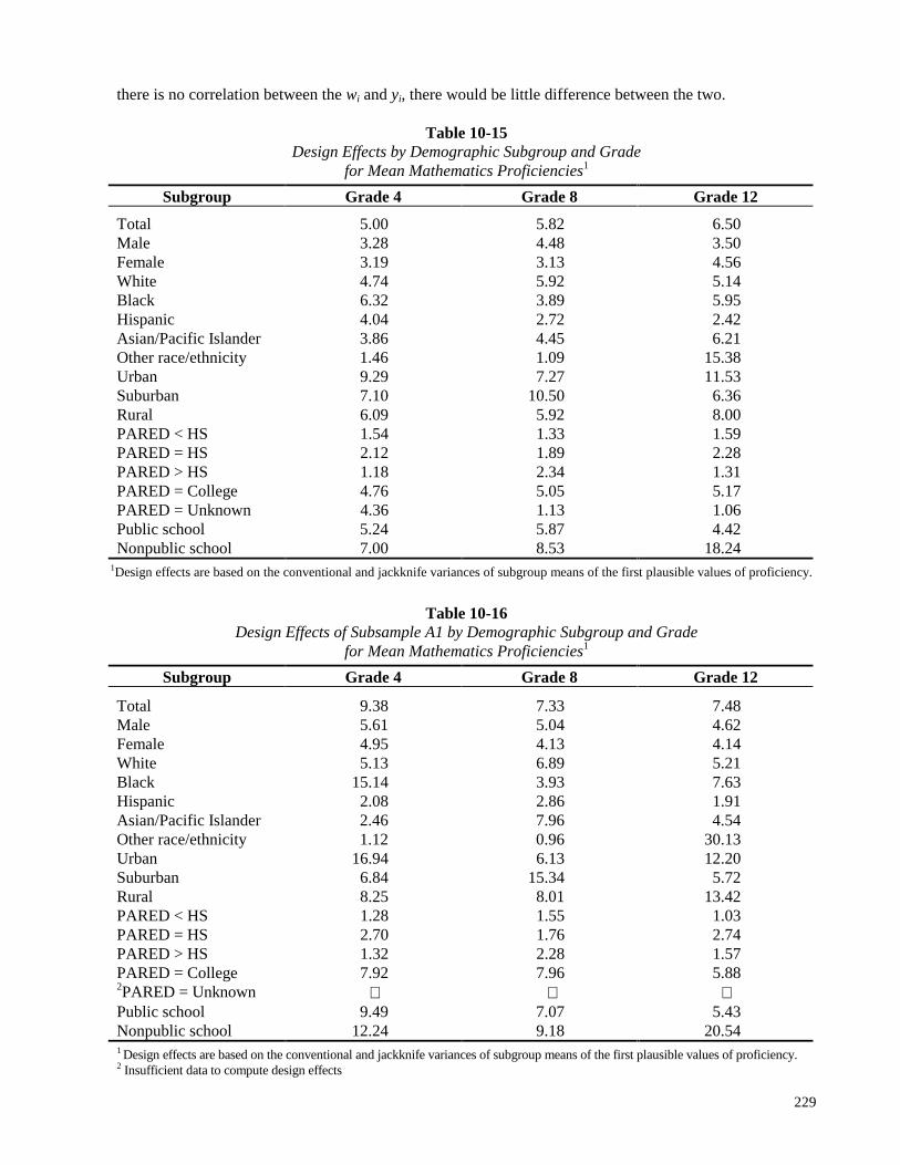
229

there is no correlation between the wi and yi, there would be little difference between the two.

Table 10-15Design Effects by Demographic Subgroup and Grade

for Mean Mathematics Proficiencies1

Subgroup Grade 4 Grade 8 Grade 12

Total 5.00 5.82 6.50Male 3.28 4.48 3.50Female 3.19 3.13 4.56White 4.74 5.92 5.14Black 6.32 3.89 5.95Hispanic 4.04 2.72 2.42Asian/Pacific Islander 3.86 4.45 6.21Other race/ethnicity 1.46 1.09 15.38Urban 9.29 7.27 11.53Suburban 7.10 10.50 6.36Rural 6.09 5.92 8.00PARED < HS 1.54 1.33 1.59PARED = HS 2.12 1.89 2.28PARED > HS 1.18 2.34 1.31PARED = College 4.76 5.05 5.17PARED = Unknown 4.36 1.13 1.06Public school 5.24 5.87 4.42Nonpublic school 7.00 8.53 18.24

1Design effects are based on the conventional and jackknife variances of subgroup means of the first plausible values of proficiency.

Table 10-16Design Effects of Subsample A1 by Demographic Subgroup and Grade

for Mean Mathematics Proficiencies1

Subgroup Grade 4 Grade 8 Grade 12

Total 9.38 7.33 7.48Male 5.61 5.04 4.62Female 4.95 4.13 4.14White 5.13 6.89 5.21Black 15.14 3.93 7.63Hispanic 2.08 2.86 1.91Asian/Pacific Islander 2.46 7.96 4.54Other race/ethnicity 1.12 0.96 30.13Urban 16.94 6.13 12.20Suburban 6.84 15.34 5.72Rural 8.25 8.01 13.42PARED < HS 1.28 1.55 1.03PARED = HS 2.70 1.76 2.74PARED > HS 1.32 2.28 1.57PARED = College 7.92 7.96 5.882PARED = Unknown Public school 9.49 7.07 5.43Nonpublic school 12.24 9.18 20.541 Design effects are based on the conventional and jackknife variances of subgroup means of the first plausible values of proficiency.2 Insufficient data to compute design effects

230

Table 10-17Design Effects of Subsample A2 by Demographic Subgroup and Grade

for Mean Mathematics Proficiencies1

Subgroup Grade 4 Grade 8 Grade 12

Total 7.95 3.98 5.98Male 4.75 3.50 3.19Female 4.78 2.02 5.32White 4.39 3.95 3.50Black 3.43 1.80 1.92Hispanic 3.26 2.31 3.00Asian/Pacific Islander 3.92 2.07 1.61Other race/ethnicity 0.60 1.41 2.05Urban 7.25 6.77 5.53Suburban 13.77 4.80 5.36Rural 4.24 4.25 3.94PARED < HS 1.44 1.52 1.76PARED = HS 1.81 2.18 1.41PARED > HS 1.19 0.92 1.89PARED = College 5.55 2.10 3.272PARED = Unknown Public school 7.79 4.02 5.08Nonpublic school 5.99 7.58 6.081 Design effects are based on the conventional and jackknife variances of subgroup means of the first plausible values of proficiency.2 Insufficient data to compute design effects

Table 10-18Design Effects of Subsample B1 by Demographic Subgroup and Grade

for Mean Mathematics Proficiencies1

Subgroup Grade 4 Grade 8 Grade 12

Total 2.88 1.23 1.77Male 2.42 1.38 1.38Female 1.31 1.15 1.98White 1.95 1.54 1.10Black 1.60 0.98 1.77Hispanic 3.73 0.81 0.78Asian/Pacific Islander 1.90 0.80 8.32Other race/ethnicity 0.87 1.13 13.01Urban 3.96 1.26 1.91Suburban 2.76 1.55 1.19Rural 1.67 1.27 1.86PARED < HS 1.38 0.69 1.46PARED = HS 1.46 0.98 0.89PARED > HS 1.21 0.98 1.21PARED = College 1.45 2.00 0.722PARED = Unknown Public school 2.85 1.10 1.49Nonpublic school 0.31 0.35 5.991 Design effects are based on the conventional and jackknife variances of subgroup means of the first plausible values of proficiency.2 Insufficient data to compute design effects

231

Table 10-19Design Effects by Demographic Subgroup and Grade

for Mean Science Proficiencies1

Subgroup Grade 4 Grade 8 Grade 12

Total 3.83 4.98 4.80Male 2.43 3.35 3.77Female 2.43 4.23 3.25White 3.71 5.09 4.73Black 4.17 2.01 2.79Hispanic 3.08 3.57 4.60Asian/Pacific Islander 4.00 3.07 2.81Other race/ethnicity 2.45 2.38 2.18Urban 11.40 7.17 11.86Suburban 13.97 8.51 8.60Rural 6.17 6.66 5.07PARED < HS 1.23 1.75 1.91PARED = HS 1.79 2.35 3.11PARED > HS 1.16 1.66 2.43PARED = College 2.64 4.50 2.95PARED = Unknown 2.77 3.72 1.74Public school 3.97 4.43 4.94Nonpublic school 5.23 9.31 6.961 Design effects are based on the conventional and jackknife variances of subgroup means of the first plausible values of proficiency.

Table 10-20Design Effects by Demographic Subgroup and Age Averaged Over Mean

Reading and Writing Proficiencies for the Reading and Writing Long-Term Trend Samples1

Subgroup Age 9 Age 13 Age 17

Total 1.86 2.13 2.13Male 1.08 1.81 1.79Female 2.00 1.85 2.08White 1.51 1.24 1.84Black 1.31 3.93 2.48Hispanic 2.17 1.98 1.21Asian/Pacific Islander 1.53 1.78 2.22Other race/ethnicity 1.23 1.75 3.75Urban 2.16 6.65 2.58Suburban 3.37 4.35 2.08Rural 3.74 3.33 8.14PARED < HS 0.89 1.66 1.06PARED = HS 1.68 1.09 1.03PARED > HS 1.12 1.22 1.86PARED = College 1.21 2.09 1.42PARED = Unknown 2.08 2.04 0.68Public school 2.05 1.89 2.41Nonpublic school 1.96 2.28 2.161 Design effects are based on the conventional and jackknife variances of subgroup means of the first plausible values of proficiency.

232

Table 10-21Design Effects by Demographic Subgroup and Age Averaged Over Mean

Mathematics and Science Proficiencies for the Mathematics and Science Long-Term Trend Samples1

Subgroup Age 9 Age 13 Age 17

Total 3.02 3.54 2.04Male 2.88 1.76 1.86Female 1.37 2.83 1.45White 2.49 3.95 2.04Black 2.83 1.79 1.17Hispanic 2.06 2.06 1.75Asian/Pacific Islander 2.29 2.72 1.71Other race/ethnicity 1.79 2.18 1.8Urban 4.42 6.18 5.16Suburban 4.36 7.73 2.42Rural 6.32 8.52 6.35PARED < HS 0.84 2.09 1.8PARED = HS 1.51 1.79 2.39PARED > HS 1.88 1.08 1.7PARED = College 2.67 2.14 1.77PARED = Unknown 0.71 1.86 1.47Public school 2.72 3.57 1.86Nonpublic school 4.36 10.89 4.741 Design effects are based on the conventional and jackknife variances of subgroup means of the first plausible values of proficiency.

Table 10-22Average Design Effects by Demographic Subgroup for Mean

State Mathematics Proficiencies Averaged Across State Samples1

Subgroup Grade 4 Grade 8

Total 4.15 3.45Male 2.65 2.36Female 2.66 2.36White 3.06 2.56Black 1.98 1.93Hispanic 1.84 1.59Asian/Pacific Islander 1.57 1.40Other race/ethnicity 1.63 1.76Urban 5.99 4.88Suburban 4.23 3.59Rural 4.19 3.08PARED < HS 1.37 1.26PARED = HS 1.65 1.79PARED > HS 1.37 1.44PARED = College 2.89 2.37PARED = Unknown 2.13 1.47Public school 4.02 3.42Nonpublic school 7.06 5.601 Design effects are based on the conventional and jackknife variances of subgroup meansof the first plausible values of proficiency.

233

Table 10-23Average Design Effects by Demographic Subgroup for MeanState Science Proficiencies Averaged Across State Samples1

Subgroup Grade 8

Total 3.53Male 2.43Female 2.33White 2.55Black 1.92Hispanic 1.63Asian/Pacific Islander 1.34Other race/ethnicity 1.70Urban 5.13Suburban 3.52Rural 2.99PARED < HS 1.34PARED = HS 1.75PARED > HS 1.45PARED = College 2.26PARED = Unknown 1.51Public school 3.41Nonpublic school 6.50

1 Design effects are based on the conventional and jackknife variances ofsubgroup means of the first plausible values of proficiency.

Table 10-24Within-Grade Mean, Median, and Upper Quartile of the Distribution of Design Effects

for National Main Assessments by Subject Area and Across Subject Areas

Statistic Grade 4 Grade 8 Grade 12

Mean Mathematics Proficiencies(Distribution Across Demographics Subgroups)

Upper Quartile 6.09 5.92 6.50Mean 4.48 4.52 6.09Median 4.88 5.44 6.08

Mean Science Proficiencies(Distribution Across Demographics Subgroups)

Upper Quartile 4.17 5.09 4.94Mean 4.25 4.37 4.36Median 3.90 4.47 4.67

Across Subject Areas(Distribution Across Subject Areas and Demographic Subgroups)

Upper Quartile 5.24 5.92 6.36Mean 4.36 4.45 5.23Median 3.92 4.33 4.58

234

Table 10-25Mean, Median, and Upper Quartile of the Across-State Average Design Effects

for Mean State Mathematics Proficiency (Distribution Across Demographic Subgroups)

Statistics Grade 4 Grade 8

Upper Quartile 4.15 3.42Mean 3.02 2.57Median 2.66 2.36

Table 10-26Mean, Median, and Upper Quartile of the Across-State Average Design Effects

for Mean State Science Proficiency (Distribution Across Demographic Subgroups)

Statistics Grade 8

Upper Quartile 3.41Mean 2.63Median 2.30

Table 10-27Mean, Median, and Upper Quartile of the Across-State Average Design Effects

for Mean State Proficiency (Distribution Across Demographic Subgroups and Across Subjects)

Statistics Grade 4 Grade 8

Upper Quartile 4.15 3.42Mean 3.02 2.60Median 2.66 2.35

Table 10-28Mean, Median, and Upper Quartile of the Distribution of Design Effects

for the Long-Term Trend Samples1

Statistic Age 9 Age 13 Age 17

Reading and Writing Long-Term Trend(Distribution Across Demographic Subgroups of Averageof Design Effects for Reading and Writing Mean Proficiencies)

Upper Quartile 2.08 3.09 2.48Mean 1.81 2.44 2.40Median 1.67 1.94 2.08

Mathematics and Science Long-Term Trend(Distribution Across Demographic Subgroups of Averageof Design Effects for Mathematics and Science Mean Proficiencies)

Upper Quartile 3.02 3.95 2.39Mean 2.70 3.70 2.42Median 2.58 2.45 1.83

1 Design effects are based on the conventional and jackknife variances of subgroup means of the first plausible values ofproficiency.

235

Chapter 11

SCALING PROCEDURES1

Nancy L. Allen, Eugene G. Johnson, Robert J. Mislevy, and Neal ThomasEducational Testing Service

11.1 INTRODUCTION

The primary method by which results from the 1996 National Assessment of EducationalProgress (NAEP) were disseminated was scale-score reporting. With scaling methods, the performanceof a sample of students in a subject area or subarea can be summarized on a single scale or series ofscales even when different students have been administered different items. This chapter presents anoverview of the scaling methodologies employed in the analyses of the data from NAEP surveys ingeneral and from the 1996 assessment in particular. Details of the scaling procedures specific to thesubject areas of science, mathematics, reading, and writing are presented in Chapters 12 through 17.

11.2 BACKGROUND

The basic information from an assessment consists of the responses of students to the itemspresented in the assessment. For NAEP, these items are constructed to measure performance on sets ofobjectives developed by nationally representative panels of learning area specialists, educators, andconcerned citizens. Satisfying the objectives of the assessment and ensuring that the tasks selected tomeasure each goal cover a range of difficulty levels typically require many items. For example, themathematics assessment required 164 items at grade 8. Depending on the subject areas, a mixture ofmultiple-choice, short constructed-response, and extended constructed-response items were used.Multiple-choice and short constructed-response items were used in all assessments but writing. Extendedconstructed-response items, scored on a multipoint scale, were presented in the main mathematics andscience assessments and in the long-term trend writing assessment. To reduce student burden, eachassessed student was presented only a fraction of the full pool of items through multiple matrix samplingprocedures.

The most direct manner of presenting the assessment results is to report separate statistics foreach item. However, because of the vast amount of information, having separate results for each of theitems in the assessment pool hinders the comparison of the general performance of subgroups of thepopulation. Item-by-item reporting masks similarities in trends and subgroup comparisons that arecommon across items.

An obvious summary of performance across a collection of items is the average of the separateitem scores. The advantage of averaging is that it tends to cancel out the effects of peculiarities in items

1 Nancy L. Allen is responsible for the psychometric and statistical analysis of national and state NAEP data. Eugene G. Johnsonis a senior psychometrician, contributing to the design of NAEP and to discussions of sampling issues. Previously he wasresponsible for the psychometric and statistical analysis of NAEP data. Robert J. Mislevy is a technical consultant contributing inthe area of item response theory. Neal Thomas was a technical consultant to the NAEP analysis staff, contributing in the area ofimputed values.

236

that can affect item difficulty in unpredictable ways. Furthermore, averaging makes it possible tocompare more easily the general performances of subpopulations.

Despite their advantages, there are a number of significant problems with average item scores.First, the interpretation of these results depends on the selection of the items; the selection of easy ordifficult items could make student performance appear to be overly high or low. Second, the averagescore is related to the particular items comprising the average, so that direct comparisons in performancebetween subpopulations require that those subpopulations have been administered the same set of items.Third, because this approach limits comparisons to average scores on specific sets of items, it providesno simple way to report trends over time when the item pool changes. Finally, direct estimates ofparameters or quantities such as the proportion of students who would achieve a certain score across theitems in the pool are not possible when every student is administered only a fraction of the item pool.While the average score across all items in the pool can be readily obtained (as the average of theindividual item scores), statistics that provide distributional information, such as quantiles of thedistribution of scores across the full set of items, cannot be readily obtained without additionalassumptions.

These limitations can be overcome by the use of response scaling methods. If several itemsrequire similar skills, the regularities observed in response patterns can often be exploited to characterizeboth respondents and items in terms of a relatively small number of variables. These variables include arespondent-specific variable, called proficiency, which quantifies a respondent’s tendency to answeritems correctly (or, for multipoint items, to achieve a certain score) and item-specific variables thatindicate characteristics of the item such as its difficulty, effectiveness in distinguishing betweenindividuals with different levels of proficiency, and the chances of a very low proficiency respondentcorrectly answering a multiple-choice item. (These variables are discussed in more detail in the nextsection.) When combined through appropriate mathematical formulas, these variables capture thedominant features of the data. Furthermore, all students can be placed on a common scale, even thoughnone of the respondents takes all of the items within the pool. Using the common scale, it becomespossible to discuss distributions of proficiency in a population or subpopulation and to estimate therelationships between proficiency and background variables.

It is important to point out that any procedure of aggregation, from a simple average to a complexmultidimensional scaling model, highlights certain patterns at the expense of other potentially interestingpatterns that may reside within the data. Every item in a NAEP survey is of interest and can provideuseful information about what young Americans know and can do. The choice of an aggregationprocedure must be driven by a conception of just which patterns are salient for a particular purpose.

The scaling for the main assessments in mathematics and science was carried out separatelywithin the content strands or fields specified in the frameworks for those subjects, respectively. Thisscaling within subareas was done because it was anticipated that different patterns of performance ordifferent trends over time might exist for these essential subdivisions of the subject areas. By creating aseparate scale for each of these content areas, potential differences in subpopulation performancebetween the content areas are preserved.

The creation of a series of separate scales to describe performance within a subject area does notpreclude the reporting of a single index of overall performance in the subject area��that is, an overallsubject area composite. A composite is computed as the weighted average of the content area scales,where the weights correspond to the relative importance given to each content area as defined by theframework. The composite provides a global measure of performance within the subject area, while the

237

constituent content area scales allow the measurement of important interactions within educationallyrelevant subdivisions of the subject area.

11.3 SCALING METHODOLOGY

This section reviews the scaling models employed in the analyses of data of the 1996 assessment,and the multiple imputation or “plausible values” methodology that allows such models to be used withNAEP’s sparse item-sampling design. The reader is referred to Mislevy (1991) for an introduction toplausible values methods and a comparison with standard psychometric analyses, to Donoghue (1994),Mislevy, Johnson and Muraki (1992), and Beaton and Johnson (1992) for additional information on howthe models are used in NAEP, and to Rubin (1987) for the theoretical underpinnings of the approach. Itshould be noted that the imputation procedure used by NAEP is a mechanism for providing plausiblevalues for the unobserved proficiencies and not for filling in blank responses to background or cognitivevariables.

While the NAEP procedures were developed explicitly to handle the characteristics of NAEPdata, they build on other research, and are paralleled by other researchers. See, for example Dempster,Laird, and Rubin (1977); Little and Rubin (1983, 1987); Andersen (1980); Engelen (1987); Hoijtink(1991); Laird (1978); Lindsey, Clogg, and Grego (1991); Zwinderman (1991); Tanner and Wong (1987);and Rubin (1987, 1991).

11.3.1 The Scaling Models

Three distinct scaling models, depending on item type and scoring procedure, were used in theanalysis of the data from the 1996 assessment. Each of the models is based on item response theory (IRT;e.g., Lord, 1980). Each is a “latent variable” model, defined separately for each of the scales, whichexpresses respondent’s tendencies to achieve certain scores (such as correct/incorrect) on the itemscontributing to a scale as a function of a parameter that is not directly observed, called proficiency on thescale.

A three-parameter logistic (3PL) model was used for the multiple-choice items (which werescored correct/incorrect). The fundamental equation of the 3PL model is the probability that a personwhose proficiency on scale k is characterized by the unobservable variable �k will respond correctly toitem j:

P x a b c cc

a bPj k j j j j

j

j k jj k� � � �

� � ��1

1

1 1 71�

��, , ,

exp .,� � � �

� � � � (11.1)

where

xj is the response to item j, 1 if correct and 0 if not;

aj where aj>0, is the slope parameter of item j, characterizing its sensitivity toproficiency;

bj is the threshold parameter of item j, characterizing its difficulty; and

cj where 0�cj<1, is the lower asymptote parameter of item j, reflecting the chances ofstudents of very low proficiency selecting the correct option.

238

Further define the probability of an incorrect response to the item as

P P x a b c Pj j k j j j j k0 10 1� � � �� �, , , .� � � � (11.2)

A two-parameter logistic (2PL) model was used for the short constructed-response items thatwere scored correct or incorrect. The form of the 2PL model is the same as Equations (11.1) and (11.2)with the cj parameter fixed at zero.

In addition to the multiple-choice and short constructed-response items, a number of extendedconstructed-response items were presented in the assessments of mathematics and science; and onlyextended constructed-response items were presented in the long-term trend writing assessment. Each ofthese items was scored on a multipoint scale with potential scores ranging from 0 to 3 or from 0 to 4.Some short constructed-response items were scored on a three-point scale (0-2). Items that are scored ona multipoint scale are referred to as polytomous items, in contrast with the multiple-choice and shortconstructed-response items, which are scored correct or incorrect and referred to as dichotomous items.

The polytomous items were scaled using a generalized partial credit model (Muraki, 1992). Thefundamental equation of this model is the probability that a person with proficiency �k on scale k willhave, for the jth item, a response xj that is scored in the ith of mj ordered score categories:

P x i a b d d

a b d

a b d

Pj k j j j j m

j k j j v

v

i

j k j j v

v

g

g

m ji kj j� �

� ����

�

� ����

��

-

=

==

-

�

���

�

��, , , , ,..., ,

exp . ,

exp . ,1 1

0

00

1

1 7

1 7� �

� �

� �� � (11.3)

where

mj is the number of categories in the response to item j

xj is the response to item j, with possibilities 0,1,...,mj-1

aj is the slope parameter;

bj is the item location parameter characterizing overall difficulty; and

dj,i is the category i threshold parameter (see below).

Indeterminacies in the parameters of the above model are resolved by setting dj,0 = 0 and setting

dj i

i

mj

, .�=

-

� 01

1

Muraki (1992) points out that bj - dj,i is the point on the �k scale at which the plots of Pj,i-1(�k)

and Pji(�k) intersect and so characterizes the point on the �k scale at which the response to item j hasequal probability of falling in response category i-1 and falling in response category i.

When mj = 2, so that there are two score categories (0,1), it can be shown that Pji(�k) of Equation(11.3) for i=0,1 corresponds respectively to Pj0(�k) and Pj1(�k) of the 2PL model (Equations (11.1) and(11.2) with cj=0).

239

Close examination of the 3PL and generalized partial credit models indicate that both modelshave a linear indeterminacy of the theta scale. In other words, if the item parameters were estimated in adifferent metric, the value of �k could be transformed to make (11.1) and (11.3) true. For the purposes ofreporting item parameter estimates and other intermediary estimates, the linear indeterminacies apparentin (11.1) and (11.3) may be resolved by an arbitrary choice of the origin and unit size in a given scale. Inmost cases, a provisional scale standardizing the theta distribution to have mean 0 and standard deviation1 is employed. Final results for each content area were linearly transformed from the � scale to a 0-to-500 (for mathematics) or a 0-to-300 scale (for science), as described in the subject area chapters in thisreport.

A basic assumption of item response theory is the conditional independence of the responses byan individual to a set of items, given the individual’s proficiency. That is, conditional on theindividual’s��k, the joint probability of a particular response pattern x = (x1,...,xn) across a set of n itemsis simply the product of terms based on (11.1), (11.2), and (11.3):

P x item parameters Pk ji ku

i

m

j

nji

j

� �,� � � ��=

-

=

��0

1

1

(11.4)

where Pji(�k) is of the form appropriate to the type of item (dichotomous or polytomous), mj is equal to 2for the dichotomously scored items, and uji is an indicator variable defined by

uif response x is incategoryi

otherwiseji

j� ��

1

0

It is also typically assumed that response probabilities are conditionally independent ofbackground variables (y), given �k, or

P x item parameters y p x item parametersk k� �, , , .� � � �� (11.5)

After x has been observed, equation 11.4 can be viewed as a likelihood function, and provides abasis for inference about �k or about item parameters. Estimates of item parameters were obtained by theNAEP BILOG/PARSCALE program, which combines Mislevy and Bock’s (1982) BILOG and Murakiand Bock’s (1991) PARSCALE computer programs2, and which concurrently estimates parameters for allitems (dichotomous and polytomous). Donoghue (1994) reports on the effect of having both dichotomousand polytomous items within a scale. The item parameters are then treated as known in subsequentcalculations. In subject areas with multiple scales (main mathematics and science), the parameters of theitems constituting each of the separate scales were estimated independently of the parameters of the otherscales. Once items have been calibrated in this manner, a likelihood function for the proficiency �k isinduced by a vector of responses to any subset of calibrated items, thus allowing �k-based inferencesfrom matrix samples. The likelihood function for the proficiency �k is called the posterior distribution ofthe thetas for each student.

In almost all NAEP IRT analyses, missing responses at the end of each block of items a studentwas administered were considered “not reached,” and treated as if they had not been presented to therespondent. Missing responses to dichotomous items before the last observed response in a block wereconsidered intentional omissions, and treated as fractionally correct at the value of the reciprocal of the

2 See Muraki and Bock (1997) for the current version of PARSCALE.

240

number of response alternatives, if the item was a multiple-choice item. These conventions are discussedby Mislevy and Wu (1988). With regard to the handling of not-reached items, Mislevy and Wu found thatignoring not-reached items introduces slight biases into item parameter estimation when not-reacheditems are present and speed is correlated with ability. With regard to omissions, they found that themethod described above provides consistent limited-information maximum likelihood estimates of itemand ability parameters under the assumption that respondents omit only if they can do no better thanresponding randomly.

Occasionally, extended constructed-response items were the last item in a block of items.Because considerably more effort was required of the student to answer these items, nonresponse to anextended constructed-response item at the end of a block was considered an intentional omission (andscored as the lowest category, 0) unless the student also did not respond to the item immediatelypreceding that item. In that case, the extended constructed-response item was considered not reached andtreated as if it had not been presented to the student.

Although the IRT models are employed in NAEP only to summarize performance, a number ofchecks are made to detect serious violations of the assumptions underlying the models. Checks are madeto detect multidimensionality of the construct being measured and certain condition dependencies. DIFanalyses are used to examine issues of dimensionality, and what are called �2 statistics in the IRTliterature are used to flag responses with serious departures from the IRT model. The latter statisticsmight better be called item fit statistics since they do not really have �2 distributions. These checksinclude comparisons of empirical and theoretical item response functions to identify items for which theIRT model may provide a poor fit to the data. When warranted, remedial efforts, such as collapsingcategories of polytomous items or combining items into a single item, are made to mitigate the effects ofsuch violations on inferences.

Scaling areas in NAEP are determined a priori by grouping items into content areas for whichoverall performance is deemed to be of interest, as defined by the frameworks developed by the NationalAssessment Governing Board (NAGB). A proficiency scale �k is defined a priori by the collection ofitems representing that scale. What is important, therefore, is that the models capture salient informationin the response data to effectively summarize the overall performance on the content area of thepopulations and subpopulations being assessed in the content areas. NAEP has routinely conducteddifferential item functioning (DIF) analyses to guard against potential biases in making subpopulationcomparisons based on the proficiency distributions.

The local independence assumption embodied in Equation (11.4) implies that item responseprobabilities depend only on � and the specified item parameters, and not on the position of the item inthe booklet, the content of items around an item of interest, or the test-administration and timingconditions. However, these effects are certainly present in any application. The practical question iswhether inferences concerning aggregate performance in the scaling area that are based on the IRTprobabilities obtained via (11.4) are robust with respect to the ideal assumptions underlying the IRTmodel. Our experience with the 1986 NAEP reading anomaly (Beaton & Zwick, 1990) has shown that formeasuring small changes over time, changes in item context and speededness conditions can lead tounacceptably large random error components. These can be avoided by presenting items used to measurechange in identical test forms, with identical timings and administration conditions. Thus, we do notmaintain that the item parameter estimates obtained in any particular booklet configuration areappropriate for other conceivable configurations. Rather, we assume that the parameter estimates arecontext-bound. This is the reason that the long-term trend booklets and administration procedures havenot changed since the early 1980s and only a limited number of blocks of items are released after eachmain assessment cycle. It was also the reason we prefer common population equating to common item

241

equating whenever equivalent random samples are available for linking. In common item equating, itemsare assumed to be measuring exactly the same thing for two or more populations, despite any differencesin context or administration. In common population equating, results for two or more samples from thesame population are matched to one another when linking the scales. Therefore, the data from the StateAssessment were calibrated separately from the national NAEP data. In this case, the administrationprocedures differed somewhat between the State Assessment and the national NAEP.

In practice, PARSCALE item fit statistics are used as a way to identify items that need furtherexamination. Most of the statistics of this type that are available for use in this setting have distributionsthat are unknown. Therefore, they cannot be used for final decisions about the fit of the items to the IRTmodel. Because of the lack of statistical tests for IRT model fit, the fit of the IRT models to the observeddata was examined within each scale by comparing the empirical item response functions (IRFs) with thetheoretical curves. The primary means of accomplishing this is to generate plots of empirical versustheoretical item response curves. The theoretical curves are plots of the response functions based on theestimates of the item parameters. The empirical proportions are calculated from the posteriordistributions of the thetas for each student who received the item. For dichotomous items, the sum of thevalues of the posterior distributions at a point on the theta scale for each student who answered an itemcorrectly plus the sum of a fractional portion of the values of the posterior distribution at that point on thetheta scale for each student who omitted the item is parallel in meaning to the number of students whoactually answered the item correctly plus a fraction of the number of students who omitted the item. Thesum of the values of the posterior distributions for all students receiving the item at each point on thetheta scale is parallel in meaning to the empirical number of students at that point on the theta scale whoreceived the item. The plotted values are sums of these individual posteriors at each point on the thetascale for those who got the item correct plus a fraction of the omitters divided by the sum of theposteriors of those administered the item, in the case of dichotomous items, and for those who scored inthe category of interest over the sum for those who received the item, in the case of polytomous items.

Figure 11-1 contains a plot of the empirical and theoretical IRFs for a dichotomous item. In theplot, the horizontal axis represents the theta (proficiency) scale, the vertical axis represents theprobability of a correct response. The solid curve is the theoretical IRF based on the item parameterestimates and Equation (11.1). The centers of the diamonds represent the empirical proportions correct asdescribed above. The size of the diamonds are proportional to the sum of the posteriors at each point onthe theta scale for all of those who received the item; this is related to the number of studentscontributing to the estimation of that empirical proportion correct.

Figure 11-2 contains a plot of the empirical and theoretical IRFs for a polytomous item from the1997 Arts (Theatre) National Assessment. As for the dichotomous item plot in Figure 11-1, thehorizontal axis represents the proficiency scale, but the vertical axis represents the probability of havinga response fall in each category. The solid curves are the theoretical IRFs based on the item parameterestimates and Equation (11.3). The centers of the diamonds represent the empirical proportions ofstudents with responses in each category and are proportional to the sum of the posteriors at each pointon the theta scale for the students who received the item.

For good fitting items, the empirical and theoretical curves are close together. Therefore, itemsfor which this is not true are examined carefully. Examples of plots for specific items are provided in thesubject-area chapters. When the same items are presented in two assessment years, the empirical curvesfor the two years can be compared. Normally, these curves differ somewhat due to the sampling ofstudents for each of the two years. Figure 12-1 contains a plot for an item with curves of this type. Whenthe empirical curves differ dramatically, one cause might be a change in the meaning of the item due toinstructional or societal changes across the years. This type of item is ordinarily treated as two different

242

items—one for each of the assessment years. Figure 12-4 contains the plot for an item that has beentreated in this way.

To summarize, using current methodologies in psychometrics, assumption of conditionalindependence and the assumption that the data fit the models in Equations 11.1 and 11.3 are examinedand controlled in NAEP in several ways. They are examined by considering tests of DIF, item fitstatistics, and plots of empirical and theoretical IRFs. They are controlled by treating missing and “notreached” responses in reasonable ways, maintaining the context and administration of items acrossassessments, collapsing categories of polytomous items when appropriate, combining items into a singleitem, or making decisions about the inclusion or exclusion of an item in a scale based on data. Theidentification and amelioration of violations of IRT assumptions is an area of ongoing research ineducational measurement.

Figure 11-1Example Cross-Sectional Dichotomous Item (R016102, Age 13/Grade 8)

Exhibiting Good Model Fit*

*Note: The plot compares empirical and model-based estimates of the item response function(IRF). The smooth curve represents the model-based estimate at each provisional proficiencylevel. The diamonds represent the empirical proportion of 1994 age 13/grade 8 studentsanswering correctly at each point on the theta scale.

243

Figure 11-2Example Polytomous Item (HC00004, Grade 8) Exhibiting Good Model Fit*

*Note: The plot compares empirical and model-based estimates of the item categoryresponse functions (ICRFs). The smooth curve represents the model-based estimate ateach provisional proficiency level. The diamonds represent the empirical proportion of1997 grade 8 students with responses in each category at each point on the theta scale.

11.3.2 An Overview of Plausible Values Methodology

Item response theory was developed in the context of measuring individual examinees’ abilities.In that setting, each individual is administered enough items (often 60 or more) to permit precise

estimation of his or her �, as a maximum likelihood estimate, �� , for example. Because the uncertaintyassociated with each � is negligible, the distribution of �, or the joint distribution of � with other

variables, can then be approximated using an individual’s �� values as if they were � values.

This approach breaks down in the assessment setting when, in order to provide broader contentcoverage in limited testing time, each respondent is administered relatively few items in a subject areascale. A first problem is that the uncertainty associated with individual �s is too large to ignore, and the

features of the �� distribution can be seriously biased as estimates of the � distribution. (The failure ofthis approach was verified in early analyses of the 1984 NAEP reading survey; see Wingersky, Kaplan,& Beaton, 1987.) A second problem, occurring even with test lengths of 60, arises when test forms varyacross and within assessments as to the numbers, formats, and content of the test items. The measurement

error distributions thus differ even if underlying � distributions do not, causing �� distributions to exhibit

244

spurious changes and comparisons in apparent population distributions��easily greater than actualdifferences over time or across groups. Although this latter problem is avoided in traditional standardizedtesting by presenting students with parallel test forms, controlled tightly across time and groups, the sameconstraints cannot be imposed in the design and data-collection phases of the present NAEP. Plausiblevalues were developed as a way to estimate key population features consistently, and approximate othersno worse than standard IRT procedures would, even when item booklet composition, format, and contentbalances change over time. A detailed development of plausible values methodology is given in Mislevy(1991). Along with theoretical justifications, that paper presents comparisons with standard procedures,discussions of biases that arise in some secondary analyses, and numerical examples.

The following provides a brief overview of the plausible values approach, focusing on itsimplementation in the 1996 NAEP analyses.

Let y represent the responses of all sampled examinees to background and attitude questions,along with variables based on the sampling design such as the school where the student is enrolled, andlet � represent the vector of proficiency values. If � were known for all sampled examinees, it would bepossible to compute a statistic t(�,y), such as a scale or composite subpopulation sample mean, a samplepercentile point, or a sample regression coefficient, to estimate a corresponding population quantity T. Afunction U(�,y)��e.g., a jackknife estimate—would be used to gauge sampling uncertainty, as thevariance of t around T in repeated samples from the population.

Because the scaling models are latent variable models, however, � values are not observed evenfor sampled students. To overcome this problem, we follow Rubin (1987) by considering � as “missingdata,” and approximate t(�,y) by its expectation given (x,y), the data that actually were observed, asfollows:

t x y t y x y

t y p x y d

* , , ,

, , .

� � � �� � � �

�

� �� �

� � �(11.6)

It is possible to approximate t* using random draws from the predictive conditional distributionof the scale proficiencies given the item responses xi, background variables yi, and model parameters forsampled student i. These values are referred to as imputations in the sampling literature, and plausiblevalues in NAEP. The value of � for any respondent that would enter into the computation of t is thusreplaced by a randomly selected value from the respondent’s conditional distribution. Rubin (1987)proposes that this process be carried out several times��multiple imputations��so that the uncertaintyassociated with imputation can be quantified. The average of the results of, for example, M estimates of t,each computed from a different set of plausible values, is a Monte Carlo approximation of (11.6); thevariance among them, B, reflects uncertainty due to not observing �, and must be added to the estimatedexpectation of U(�,y), which reflects uncertainty due to testing only a sample of students from thepopulation. Section 11.5 explains how plausible values are used in subsequent analyses.

It cannot be emphasized too strongly that plausible values are not test scores for individuals inthe usual sense. Plausible values are offered only as intermediary computations for calculating integralsof the form of Equation (11.6), in order to estimate population characteristics. When the underlyingmodel is correctly specified, plausible values will provide consistent estimates of populationcharacteristics, even though they are not generally unbiased estimates of the proficiencies of theindividuals with whom they are associated. The key idea lies in the contrast between plausible values and

245

the more familiar estimates of proficiency (e.g., maximum likelihood estimate or Bayes estimate) that arein some sense optimal for each examinee: Point estimates that are optimal for individual examinees havedistributions that can produce decidedly nonoptimal (specifically, inconsistent) estimates of populationcharacteristics (Little & Rubin, 1983). Plausible values, on the other hand, are constructed explicitly toprovide consistent estimates of population effects. For further discussion see Mislevy, Beaton, Kaplan,and Sheehan (1992).

11.3.3 Computing Plausible Values in IRT-Based Scales

Plausible values for each respondent r are drawn from the predictive conditional distributionp(�r|xr,yr,�,�), where � and � are regression model parameters defined in this subsection. Thissubsection describes how, in IRT-based scales, these conditional distributions are characterized, and howthe draws are taken. An application of Bayes’ theorem with the IRT assumption of conditionalindependence produces

p x yr r r� , ,� �,� � � P x yr r r� , ,�,� � �p yr r� , �,� � � � �� P x p yr r r r� � ,�,� � (11.7)

where, for vector-valued �r, P(xr|�r) is the product over scales of the independent likelihoods induced byresponses to items within each scale, and p(�r|yr, �,�) is the multivariate��and generallynonindependent��joint density of proficiencies for the scales, conditional on the observed value yr ofbackground responses, and the parameters � and �. The provisional scales are determined by the itemparameter estimates that constrain the population mean to zero and standard deviation to one. The itemparameter estimates are fixed and regarded as population values in the computation described in thissubsection.

In the analyses of the data from the main assessments, a normal (Gaussian) form was assumed forp(�r|yr,�,�), with a common variance-covariance matrix, �, and with a mean given by a linear modelwith slope parameters, �, based on the first approximately 200 principal components of several hundredselected main-effects and two-way interactions of the complete vector of background variables. Theincluded principal components will be referred to as the conditioning variables, and will be denoted yc.(The complete set of original background variables used in the analyses of each subject area are listed inAppendix C.) The following model was fit to the data within each subject area:

� = � ’yc � (11.8)

where is multivariately normally distributed with mean zero and variance-covariance matrix �. Thenumber of principal components of the background variables used for each sample was sufficient toaccount for 90 percent of the total variance of the full set of background variables (after standardizingeach variable). As in regression analysis, � is a matrix each of whose columns is the effects for one scaleand � is the matrix variance-covariance of residuals between scales.

A model similar to (11.8) was used for the long-term trend assessments, with the difference thatyc consisted of main effects and interactions from the smaller set of background variables (rather thanprincipal components of those variables) available in the long-term trend assessments.

246

Maximum likelihood estimates of � and �, denoted by �� and �� , are obtained with extensionsof Sheehan’s (1985) MGROUP computer program using the EM algorithm described in Mislevy (1985).The EM algorithm requires the computation of the mean, �r , and variance-covariance matrix, � p

r , of thepredictive conditional distribution in (11.7) for respondent r when there are p scales within a subjectarea. For subject areas with multiple scales, the CGROUP version of the MGROUP program was used tocompute the moments using higher order asymptotic corrections to a normal approximation (Thomas,1993). For the long-term trend assessments, each of which have a single scale, the more precise butcomputationally intensive BGROUP version of MGROUP was used. BGROUP uses numeric quadratureto evaluate the predictive conditional distribution moments required by the E-step of the EM algorithmfor one- and two-dimensional applications (Thomas, 1993). For estimation of group means on a singlescale, CGROUP and BGROUP results will be nearly identical to those from the original MGROUPprogram. CGROUP and BGROUP yield better estimates of correlations between scales, and hence betterestimates of composite scale means. BGROUP will, theoretically, yield better estimates than CGROUP,but because of the heavy computational demands of the methodology used, its function is limited tobivariate scales. Hence CGROUP is used for assessments involving more than two scales.

After completion of the EM algorithm, the plausible values for all sampled respondents is drawnin the following three-step process. First, a value of � is drawn from a normal distribution with mean

being �� and variance being the variance of � .� Second, conditional on the generated value of � and the

fixed value of � = � ,� the predictive conditional distribution mean �r and the predictive conditionaldistribution variance �

r of respondent r are computed from Equation 11.7 using the EM algorithm (seeThomas, 1993). Finally, the �r are drawn independently from a multivariate normal distribution with

mean �r and variance � r approximating the distribution in (11.7). These three steps are repeated five

times producing five sets of imputation values for all sampled respondents.

11.4 INFERENCES ABOUT PROFICIENCIES

When survey variables are observed without error from every respondent, usual varianceestimators quantify the uncertainty associated with sample statistics from the only source of uncertainty,namely the sampling of respondents. Item-level statistics for NAEP cognitive items meet thisrequirement, but proficiency values do not. The IRT models used in their construction posit anunobservable proficiency variable � to summarize performance on the items in the subarea. The fact that� values are not observed even for the respondents in the sample requires additional statistical analysesto draw inferences about � distributions and to quantify the uncertainty associated with those inferences.As described above, Rubin’s (1987) multiple imputations procedures were adapted to the context oflatent variable models to produce the plausible values upon which many analyses of the data from the1996 assessment were based. This section describes how plausible values were employed in subsequentanalyses to yield inferences about population and subpopulation distributions of proficiencies.

11.4.1 Computational Procedures

Even though one does not observe the � value of respondent r, one does observe variables thatare related to it: xr, the respondent’s answers to the cognitive items he or she was administered in the areaof interest, and yr, the respondent’s answers to demographic and background variables. Suppose onewishes to draw inferences about a number T(�,Y) that could be calculated explicitly if the � and y values

247

of each member of the population were known. Suppose further that if � values were observable, wewould be able to estimate T from a sample of N pairs of � and y values by the statistic t(�,y) [where(�,y) � (�1,y1,...,�N,yN)], and that we could estimate the variance in t around T due to samplingrespondents by the function U(�,y). Given that observations consist of (xr,yr) rather than (�r,yr), we canapproximate t by its expected value conditional on (x,y), or

t* (x,y) = E[t(�,y)|x,y] = � t(�,y) p(� |x,y) d� .

It is possible to approximate t* with random draws from the conditional distributions p(�i|xi,yi),

which are obtained for all respondents by the method described in Section 11.3.3. Let ��m be the mth suchvector of plausible values, consisting of a multidimensional value for the latent variable of eachrespondent. This vector is a plausible representation of what the true � vector might have been, had webeen able to observe it.

The following steps describe how an estimate of a scalar statistic t(�,y) and its sampling variancecan be obtained from M (>1) such sets of plausible values. (Five sets of plausible values are used inNAEP analyses.)

1. Using each set of plausible values ��m in turn, evaluate t as if the plausible values

were true values of �. Denote the results �tm , for m=1,...,M. 2. Using the jackknife variance estimator defined in Chapter 10, compute the estimated

sampling variance of �tm , denoting the result Um.

3. The final estimate of t is

tt

Mm

m

M

*�

.�=

�1

4. Compute the average sampling variance over the M sets of plausible values, to

approximate uncertainty due to sampling respondents

UU

Mm

m

M

* .�=

�1

5. Compute the variance among the M estimates �tm , to approximate the between-imputation variance

Bt t

M

m

m

M

���

=

�� *

.� �� �

2

1 1

6. The final estimate of the variance of t* is the sum of two components

V U M B� � � -* .1 1� �In this equation, (1+M-1)B is the estimate of variance due to the latency of . Due to theexcessive computation that would be required, NAEP analyses did not compute and

248

average jackknife variances over all five sets of plausible values, but only on the first set.Thus, in NAEP reports, U* is approximated by U1.

11.4.2 Statistical Tests

The variance described in Section 11.4.1 is used to make statistical tests comparing NAEPresults. This section describes the relationships between these tests and the variance componentsdescribed above. Chapter 18 contains details of the hypothesis tests used in this assessment.

Suppose that if � values were observed for sampled students, the statistic (t - T)/U1/2 wouldfollow a t-distribution with d degrees of freedom. Then the incomplete-data statistic (t* - T)/V1/2 isapproximately t-distributed, with degrees of freedom (Satterthwaite, 1941; Johnson & Rust, 1993)given by

vf

M

f

d

�

��

�1

1

12 2� �

where f is the proportion of total variance due to not observing � values:

f M B V� � -1 1� � / .

When B is small relative to U*, the reference distribution for incomplete-data statistics differslittle from the reference distribution for the corresponding complete-data statistics. This is the case withmain NAEP reporting variables. If, in addition, d is large, the normal approximation can be used to flag“significant” results.

For k-dimensional t, such as the k coefficients in a multiple regression analysis, each Um and U*

is a covariance matrix, and B is an average of squares and cross-products rather than simply an average ofsquares. In this case, the quantity (T-t*) V -1 (T-t*), is approximately F distributed, with degrees offreedom equal to k and �, with � defined as above but with a matrix generalization of f:

f = (1+M-1) Trace (BV-1)/k .

By the same reasoning as used for the normal approximation for scalar t, a chi-square distribution on kdegrees of freedom often suffices for multivariate t.

11.4.3 Biases in Secondary Analyses

Statistics t* that involve proficiencies in a scaled content area and variables included in theconditioning variables yc are consistent estimates of the corresponding population values T. This includesinterrelationships among scales within a content area that have been treated in the multivariate mannerdescribed above in Section 11.3.3. Statistics involving background variables y that were not conditionedon, or relationships among proficiencies from different content strands or fields, are subject to asymptoticbiases whose magnitudes depend on the type of statistic and the strength of the relationships of thenonconditioned background variables to the variables that were conditioned on and to the proficiency ofinterest. That is, the large sample expectations of certain sample statistics need not equal the truepopulation parameters.

249

The direction of the bias is typically to underestimate the effect of nonconditioned variables. Fordetails and derivations see Beaton and Johnson (1990), Mislevy (1991), and Mislevy and Sheehan (1987,Section 10.3.5). For a given statistic t* involving one content area and one or more nonconditionedbackground variables, the magnitude of the bias is related to the extent to which observed responses xaccount for the latent variable �, and the degree to which the nonconditioned background variables areexplained by conditioning background variables. The first factor��conceptually related to testreliability��acts consistently in that greater measurement precision reduces biases in all secondaryanalyses. The second factor acts to reduce biases in certain analyses but increase it in others. Inparticular,

• High shared variance between conditioned and nonconditioned background variablesmitigates biases in analyses that involve only proficiency and nonconditionedvariables, such as marginal means or regressions.

• High shared variance exacerbates biases in regression coefficients of conditional

effects for nonconditioned variables, when nonconditioned and conditionedbackground variables are analyzed jointly as in multiple regression.

The large number of background variables that have been included in the conditioning vectors for the1996 assessments allows a large number of secondary analyses to be carried out with little or no bias, andmitigates biases in analyses of the marginal distributions of � in nonconditioned variables. Kaplan andNelson’s analysis of the 1988 NAEP reading data (some results of which are summarized in Mislevy,1991), which had a similar design and fewer conditioning variables, indicates that the potential bias fornonconditioned variables in multiple regression analyses is below 10 percent, and biases in simpleregression of such variables is below five percent. Additional research (summarized in Mislevy, 1990)indicates that most of the bias reduction obtainable from conditioning on a large number of variables canbe captured by instead conditioning on the first several principal components of the matrix of all originalconditioning variables. This procedure was adopted for the 1992, 1994, and 1996 main assessments byreplacing the conditioning effects by the first K principal components, where K was selected so that 90percent of the total variance of the full set of conditioning variables (after standardization) was captured.Mislevy (1990) shows that this puts an upper bound of 10 percent on the average bias for all analysesinvolving the original conditioning variables.

11.4.4 A Numerical Example

To illustrate how plausible values are used in subsequent analyses, this subsection gives some of thesteps in the calculation of the 1992 grade 4 reading composite mean and its estimation-error variance.This illustration is an example of the calculation of NAEP means and variances and can be used tounderstand their calculation for any NAEP assessment.

The weighted mean of the first plausible values of the reading composite for the grade 4 studentsin the sample is 217.79, and the jackknife variance of these values is 0.833. Were these values true �values, then 217.79 would be the estimate of the mean and 0.833 would be the estimation-error variance.The weighted mean of the second plausible values of the same students, however, is 217.62; the third,fourth, and fifth plausible values give weighted means of 217.74, 218.24, and 218.05. Since all of thesefigures are based on precisely the same sample of students, the variation among them is due touncertainty about the students’ �s, having observed their item responses and background variables.Consequently, our best estimate of the mean for grade 4 students is the average of the five plausiblevalues: 217.89. Taking the jackknife variance estimate from the first plausible value, 0.833, as our

250

estimate U* of sampling variance, and the variance among the five weighted means, .063, as our estimateB of uncertainty due to not observing �, we obtain as the final estimate V of total error variance 0.833 +(1+5-1) .063 = 0.908.

It is also possible to partition the estimation error variance of a statistic using these samevariance components. The proportion of error variance due to sampling students from the population isU*/V, and the proportion due to the latent nature of � is (1+M-1)B/V. The results are shown in Table 11-1.The value of U*/V roughly corresponds to reliability in classical test theory and indicates the amount ofinformation about an average individual’s � present in the observed responses of the individual. It shouldbe recalled again that the objective of NAEP is not to estimate and compare values of individualexaminees, the accuracy of which is gauged by reliability coefficients. The objective of NAEP, rather, isto estimate population and subpopulation characteristics, and the marginal estimation methods describedabove have been designed to do so consistently regardless of the values of reliability coefficients.

Table 11-1Estimation Error Variance and Related Coefficients for the 1992 Grade 4 Reading Composite

(Based on Five Plausible Values)

Proportion of Variance Due to...

U* (1+5-1)B V

StudentSampling:

U*/VLatency of �:

(1+5-1)B/V

0.833 0.076 0.908 0.92 0.08

Chapters 12 through 17 and Appendix E provide values of the proportion of variance due tosampling and due to the latent nature of � for all 1996 scales and composites for the populations as awhole and, in the appendix, for selected subpopulations. It will be seen that the proportion of variancedue to the latency of � varies somewhat among subject areas, tending to be largest for the long-term trendwriting assessment, where there is low correlation between tasks and each student responded to only oneor at most two tasks. The proportion of variance due to latency of � is smallest for the composites of themain assessment subjects, where the number of items per student is largest. Essentially, the variance dueto the latent nature of � is largest when there is less information about a student’s proficiency. (Note thedistinction between estimation error variance of a parameter estimate and the estimate of the variance ofthe � distribution. The former depends on the accuracy of measurement; the large-sample model-basedexpected value of the latter does not.) Given fixed assessment time, this decrease in information willoccur whenever the amount of information per unit time decreases as can happen when many shortconstructed-response or multiple-choice items are replaced by a few extended constructed-responseitems.

11.5 DESCRIBING STUDENT PERFORMANCE

Since its beginning, a goal of NAEP has been to inform the public about what students inAmerican schools know and can do. While the NAEP scales provide information about the distributionsof proficiency for the various subpopulations, they do not directly provide information about the meaningof various points on the scale. Traditionally, meaning has been attached to educational scales by norm-referencing��that is, by comparing students at a particular scale level to other students. In contrast,NAEP achievement levels and scale anchors describe selected points on the scale in terms of the types of

251

skills that are likely to be exhibited by students scoring at that level. The achievement level process wasapplied to the science composite. Scale anchoring of certain percentiles of the student proficiencydistribution was applied to the long-term trend assessment composite using the 1996 data. Theachievement level process for mathematics was completed for the 1990 assessment when the NAEPmathematics framework was revised, so the results were directly applied to the 1996 results. In addition,each item was mapped to a point on the scale in which it belonged, so that the content of each itemprovides information about what students at each score level can do in a probabistic sense.

11.5.1 Achievement Levels

NAGB has determined that achievement levels shall be the first and primary way of reportingNAEP results. Setting achievement levels is a method for setting standards on the NAEP assessment thatidentify what students should know and be able to do at various points on the composite. For each gradeof each subject, three levels were defined��basic, proficient, and advanced. Based on initial policydefinitions of these levels, panelists were asked to determine operational descriptions of the levelsappropriate with the content and skills assessed in the assessment. With these descriptions in mind, thepanelists were then asked to rate the assessment items in terms of the expected performance ofmarginally acceptable examinees at each of these three levels. These ratings were then mapped onto theNAEP scale to obtain the achievement level cutpoints for reporting. Further details of the achievementlevel-setting process for science appear in Appendix G.

11.5.2 Performance Descriptions Based on Composite Scales

A procedure known as scale anchoring was used to develop descriptions of student performanceat selected points on the composite scales. The scale points that were selected for anchoring reflect threelevels of knowledge and abilities corresponding to lower-, middle-, and higher-performing students foreach subject.

Around each percentile point, a band was built to define a range of scale scores. Studentsdescribed as being at a particular level were within a five percentile point range on either side of thespecified scale point. For example, the 50th percentile was defined as the region between the 45th and55th percentile points on the scale. A question was identified as anchoring at a percentile point on thescale if it was answered successfully by at least 65 percent of the students within that percentile band.(The criterion was set at 74 percent for multiple-choice questions to correct for the possibility ofanswering correctly by guessing.)

After defining the bands of the scale to be anchored, the next step in the process was to identify:(1) questions answered correctly for dichotomously scored questions, or (2) questions answered at aparticular score level for partial credit constructed-response questions. Because the extendedconstructed-response questions were scored according to four levels of performance, each extendedconstructed-response question was treated as three distinct questions corresponding to scores of Partial orbetter, Essential or better, and Extensive. These distinct score levels were then analyzed in the samemanner as questions scored dichotomously, as either correct or incorrect. Thus, for example, an extendedconstructed-response question might anchor at the 50th percentile for Partial or better responses and atthe 90th percentile for Essential or better responses.

A committee of subject area experts, including teachers for the grades involved, collegeprofessors, state curriculum supervisors, and researchers, was assembled to review the sets of questions

252

identified for each percentile band. The committee was divided into three groups, one for each grade.Each group examined and analyzed questions that anchored at the 25th, 50th, and 90th percentiles todetermine the specific knowledge and abilities associated with each question.

Committee members were also provided with the sets of questions at each grade that “did notanchor” to inform their decisions about what students could do by seeing examples of what they couldnot do. Drawing on their knowledge of the subject area, committee members were asked to summarizestudent performance by describing the knowledge, skills, and abilities demonstrated by students in eachof the score bands.

The performance descriptions are cumulative; that is, the abilities described for the lowerperforming students are considered to be among the abilities of students performing at higher points onthe scale. Therefore, the full description of student’s knowledge and abilities in the middle scale bandwould include those abilities described at the lower band. Similarly, the abilities of students performingat the higher scale band include the abilities described for students at the middle and lower bands.

11.5.3 Item Mapping Procedures

In order to map items (questions) to particular points on each subject area scale, a responseprobability convention had to be adopted that would divide those who had a higher probability of successfrom those who had a lower probability. Establishing a response probability convention has an impact onthe mapping of assessment items onto the scales. A lower boundary convention maps the items at lowerpoints along the scales, and a higher boundary convention maps the same items at higher points along thescales. The underlying distribution of skills in the population does not change, but the choice of aresponse probability convention does have an impact on the proportion of the student population that isreported as “able to do” the items on the scales.

There is no obvious choice of a point along the probability scale that is clearly superior to anyother point. If the convention were set with a boundary at 50 percent, those above the boundary would bemore likely to get an item right than get it wrong, while those below that boundary would be more likelyto get the item wrong than right. While this convention has some intuitive appeal, it was rejected on thegrounds that having a 50/50 chance of getting the item right shows an insufficient degree of mastery. Ifthe convention were set with a boundary at 80 percent, students above the criterion would have a highprobability of success with an item. However, many of the students below this criterion show some levelof achievement that would be ignored by such a stringent criterion. In particular, those in the rangebetween 50 and 80 percent correct would be more likely to get the item right than wrong, yet would notbe in the group described as “able to do” the item.

In a compromise between the 50 percent and the 80 percent conventions, NAEP has adopted tworelated response probability conventions: 74 percent for multiple-choice items (to correct for thepossibility of answering correctly by guessing), and 65 percent for constructed-response items (whereguessing is not a factor). These probability conventions were established, in part, based on an intuitivejudgment that they would provide the best picture of students’ knowledge and skills.

Some additional support for the dual conventions adopted by NAEP was provided by Huynh(1998, 1994). He examined the IRT information provided by items, according to the IRT model used inscaling NAEP items. Following Bock (1972), Huynh decomposed the item information into that providedby a correct response [Pji (�) *Ij (�)] and that provided by an incorrect response [(1-P (�)) *I (�)]. Huynhshowed that the item information provided by a correct response to a constructed-response item is

253

maximized at the point along the scale at which two-thirds of the students get the item correct (formultiple-choice items with four options, information is maximized at the point at which 75 percent getthe item correct). Maximizing the item information, I (�), rather than the information provided by acorrect response [P (�) * I (�)], would imply an item mapping criterion closer to 50 percent. Maximizingthe item information, I (�), takes into account both responses that are correct and those that are incorrect,however.

For dichotomously scored items the information function as defined by Birnbaum (1968, p. 463)is defined for the jth item as

Ia P P c

P cj

j j k j k j

j k j

�� ��

� � � � � � � �� �� ��

��

1 7

1

20 1

2

12

.,

where the notation is the same as that used in Equations (11.1) and (11.2). The item information functionwas defined by Samejima (1969) in general for polytomously scored items, and has been derived foritems scaled by the generalized partial credit model (Muraki, 1993; Donoghue, 1994) as (in a slightlydifferent, but equivalent form)

I a i P iPj j ji k

i

m

ji k

i

mj j

� � �� � � � � � � �� � �����

���

���=

-

=

-

� �1 72 2

0

1

0

1 2

. .

11.6 OVERVIEW OF THE 1996 NAEP SCALES

The following IRT scale-score analyses were carried out for the 1996 NAEP assessment:

• Mathematics: Five IRT scales linked back to the 1990 and 1992 main assessment ofmathematics and one unidimensional IRT mathematics scale linking 1996 results to resultsfrom mathematics assessments in 1973, 1976, 1982, 1986, 1990, 1992, and 1994. The firstfive scales, along with a composite scale, are associated with the 1996 main assessment,while the unidimensional scale is associated with the 1996 long-term trend assessment.

• Science: Three newly developed IRT scales for the main assessment of science and one

unidimensional scale linking 1996 results to results from science assessments in 1969, 1973,1977, 1982, 1986, 1990, 1992, and 1994. The first three scales, along with a composite scale,are associated with the 1996 main assessment, while the unidimensional scale is associatedwith the 1996 long-term trend assessment.

• Long-Term Trend Reading: One IRT scale linking 1996 results to results from reading

assessments in 1971, 1975, 1979, 1984, 1988, 1990, 1992, and 1994. This scale is associatedwith the 1996 long-term trend assessment.

• Long-Term Trend Writing: One polytomous item scale linking 1996 writing results to the

1984, 1988, 1990, 1992, and 1994 assessments. This scale is associated with the 1996 long-term trend assessment. [Please note that a review of the 1996 long-term trend writingassessment data analyses has been undertaken by NCES. Additional analyses may berequired before revised results are released.]

Details follow in Chapters 12 through 17.

255

Chapter 12

DATA ANALYSIS FOR THE MATHEMATICS ASSESSMENT1

Frank Jenkins, Hua-Hua Chang, and Edward KulickEducational Testing Service

12.1 INTRODUCTION

This chapter describes the analyses performed on the responses to the cognitive and backgrounditems in the 1996 mathematics assessment. This chapter focuses on the methods and procedures used toestimate IRT-based scale score distributions for subgroups of students. This includes a wide array oftopics, such as the scoring of constructed-response items, classical item characteristics, itemresponsetheory (IRT) analysis of mathematics scales, and estimation of subgroup means by theimputation of plausible values. The statistical bases of the IRT and plausible values methodologydescribed in this chapter are given in Chapter 11. These analyses led to the results presented in NAEP1996 Mathematics Report Card for the Nation and the States (Reese, Miller, Mazzeo, & Dossey, 1997).For a description of the state analyses, see the Technical Report of the NAEP 1996 State AssessmentProgram in Mathematics (Allen, Jenkins, Kulick, & Zelenak, 1997).

The student samples that were administered mathematics items in the 1996 national assessmentare shown in Table 12-1. (See Chapters 1 and 3 for descriptions of the target populations and the sampledesign used for the assessment.). These samples were defined only by grade (4, 8, or 12) and not by ageof the student. Data from the Math Main samples comprised the spiraled balanced incomplete block(BIB) design. The present chapter contains information about the scaling of data from these samples. Thelong-term trend analyses are presented in a separate chapter (see Chapter 15). The other samples (Math-Estimation, Math-Theme, and Math-Advanced) will be analyzed and presented in separate focus reports.A brief description of the analyses of these samples is presented in Section 12.3. Technicaldocumentation detailing the analyses of the 1996 State Assessment of mathematics is provided in theTechnical Report of the NAEP 1996 State Assessment Program in Mathematics (Allen, Jenkins, Kulick,& Zelenak, 1997).

1 Frank Jenkins was the primary person responsible for the planning, specifications, and coordination of the national mathematicsanalyses. He was assisted by Hua-Hua Chang. Data analysis and scaling were coordinated by Ed Kulick with help from Steve Wangand Xiaohui Wang and additional assistance from David Freund.

256

Table 12-1NAEP 1996 Mathematics Student Samples

SampleBookletNumber Mode

CohortAssessed Time of Testing1

NumberAssessed

4 [Math Main] 8 [Math Main]12 [Math Main]

1-26 1-26 1-26

PrintPrintPrint

Grade 4Grade 8

Grade 12

1/3/96 - 3/29/96 (Winter)1/3/96 - 3/29/96 (Winter)1/3/96 - 3/29/96 (Winter)

6,6277,1466,904

4 [Math-Estimation]8 [Math-Estimation]12 [Math-Estimation]

127127127

TapeTapeTape

Grade 4Grade 8

Grade 12

1/3/96 - 3/29/96 (Winter)1/3/96 - 3/29/96 (Winter)1/3/96 - 3/29/96 (Winter)

2,0232,1831,849

4 [Math-Theme]8 [Math-Theme]12 [Math-Theme]

128,129128,129128,129

PrintPrintPrint

Grade 4Grade 8

Grade 12

1/3/96 - 3/29/96 (Winter)1/3/96 - 3/29/96 (Winter)1/3/96 - 3/29/96 (Winter)

3,7904,0273,735

8 [Math-Advanced]12 [Math-Advanced]

130130

PrintPrint

Grade 8Grade 12

1/3/96 - 3/29/96 (Winter)1/3/96 - 3/29/96 (Winter)

2,3372,965

1 Final makeup sessions were held April 1-5, 1996.

LEGEND:

Math Mathematics Print Printed administrationMain Main spiral BIB assessment Tape Audiotape administrationEstimation Main estimation assessment Theme Assessment with theme bookletsAdvanced Assessment with advanced booklets

12.2 DESCRIPTION OF STUDENT SAMPLE, ITEMS, AND ASSESSMENTBOOKLETS

The data from the main BIB mathematics assessment (from samples 4[Math Main], 8 [MathMain], and 12[Math Main]) were used for main analyses comparing the levels of mathematicsachievement for various subgroups of the 1996 target populations. In previous assessments themathematics samples were defined as age/grade cohorts (e.g., students who were either in the fourthgrade or 9 years old). Starting with the 1996 assessment, cohorts were defined solely by grade. Thesampled students in each of these three grade cohorts were assessed in the winter. The samples in themain assessment are presented in Table 12-1.

The pool of items used in the 1996 mathematics assessment contained a range of constructed-response and multiple-choice questions measuring performance on sets of objectives (NationalAssessment Governing Board, 1994). The framework for the objectives is described in Chapter 2. A totalof 360 distinct mathematics items addressing these objectives were scaled (see Table 12-2). The numberof items per grade was 144, 164, and 165 respectively for grades 4, 8, and 12 (before scaling). Tables 12-3, 12-5, and 12-7 give, for each grade, the numbers of items by item type and block (before scaling). Foritem counts after scaling, taking into account items that were dropped or collapsed, see Tables 12-4, 12-6, and 12-8. These tables indicate that there was a nearly fourfold increase in the number ofpolytomously-scored constructed-response items over the numbers presented in the 1992 assessment. In1996, the number of items was 30 in grade 4, 30 in grade 8, and 33 in grade 12. The items were classified

257

into five content strands: numbers and operations; measurement; geometry; data analysis, statistics, andprobability; and algebra and functions. These five content strands (renamed number sense, properties,and operations; measurement; geometry and spatial sense; data analysis, statistics, and probability; andalgebra and functions in the 1996 analysis) constituted the scales used in 1996 reporting.2 The itemswere partitioned into 13 blocks and these blocks were then assigned to 26 booklets according to a BIBdesign. Each booklet contained relatively few items from each of the five categories.

Table 12-2National Main BIB: Numbers of Scaled Mathematics Items

Common Across Grade Levels, by Content Strand Scale

Grade(s)

Number Sense,Properties,

andOperations Measurement

Geometryand

SpatialSense

Data Analysis,Statistics,

andProbability

Algebraand

Functions Total

4 only 40 20 12 11 8 918 only 20 13 12 10 18 7312 only 23 11 17 22 32 1054 and 8 10 2 9 3 7 318 and 12 8 9 6 9 6 384 and 12 0 0 0 0 0 04, 8, and 12 9 3 4 3 3 22Total Grade 4 59 25 25 17 18 144Total Grade 8 47 27 31 25 34 164Total Grade 12 40 23 27 34 41 165Total 110 58 60 58 74 360

In the main samples, each student was administered a booklet containing three blocks ofmathematics cognitive items, a block of background questions common to all booklets for a particulargrade level, and a block of mathematics-related background questions common to all mathematicsbooklets for a particular grade level. At the end of each booklet there was a short block consisting of fivequestions concerning the student’s motivation and his or her perception of the difficulty of the cognitiveitems. The BIB design by which the 13 blocks of mathematics cognitive items were assigned to the 26booklets for each grade level is discussed in Chapter 4. The 13 blocks were not intended to be parallelmeasuring instruments. For example, several blocks contained only the items designed for calculatorusage, and some blocks contained items for ruler and protractor usage. In addition, the proportion ofitems sampled from the five categories were not exactly the same among the 13 blocks.

The 360 unique items were constructed according to several formats, some traditional and somemore innovative: multiple-choice items, constructed-response items scored dichotomously, constructed-response items scored polytomously, and cluster items.3 The multiple-choice items conformed to thefamiliar format of a stem followed by several possible answers, with only one answer being correct.

2 The content strand number sense, properties, and operations was called numbers and operations in the 1990 and 1992assessments. The content strand geometry and spatial sense was called geometry in the 1990 and 1992 assessments.3 A cluster item is an aggregation of a group of items (in the case of NAEP mathematics, typically three to five items) that arerelated to a single content strand, topic, or stimulus, and are developed and scored as a single unit (see Wainer & Kiely, 1987, forfurther details and examples of different types of cluster items).

258

Constructed-response items that were scored dichotomously were questions that required an open-endedresponse (e.g., explaining why the previous question was answered as it was). These questions were readby raters who determined whether or not the response was correct. Constructed-response items that werescored polytomously were open-ended questions that required several stages of reasoning or problemsolving. They were also read by raters but were given a score reflecting degree of correctness rather thansimply judged right or wrong. Cluster items were derived from a set of three to five multiple-choice itemsthat related to the same basic stem. The cluster score was the number of constituent cluster items that therespondent answered correctly.

As Table 12-3 indicates, of the 144 items at grade 4, 79 were multiple-choice items, 16 wereconstructed response items that were scored dichotomously, 48 were constructed-response items thatwere scored polytomously, and 1 was a cluster item. As shown in Table 12-5, of 163 items at grade 8, 91were multiple-choice items, 21 were constructed-response items that were scored dichotomously, 48were constructed-response items that were scored polytomously, and 3 were cluster items. For grade 12,Table 12-7 indicates that of the 166 items administered, 92 were multiple-choice items, 21 wereconstructed-response items that were scored dichotomously, 50 were constructed-response items thatwere scored polytomously, and 3 were cluster items.

Tables 12-4, 12-6, and 12-8 show comparable information for each grade after the scaling wascarried out.

Table 12-31996 NAEP Mathematics Block Composition by Content Strand

and Item Type, Grade 4, As Defined Before Scaling

Multiple-Choice

Constructed-Response Items ScoredPolytomously Cluster Total

Block Items 2-category 3-category 4-category 5-category Items Items

M3 9 4 0 0 0 0 13M4 14 0 0 0 0 0 14M5 4 0 5 0 1 0 10M6 0 7 2 2 0 0 11M7 3 0 4 0 1 0 8M8 14 0 1 0 0 0 15M9 6 2 0 0 1 1 10

M10 0 1 4 1 0 0 6M11 11 0 0 2 3 0 16M12 5 0 3 0 1 0 9M13 6 1 2 2 1 0 12M14 4 0 5 0 1 0 10M15 3 1 5 0 1 0 10Total 79 16 31 7 10 1 144

259

Table 12-41996 NAEP Mathematics Block Composition by Content Strand

and Item Type, Grade 4, As Defined After Scaling*

Multiple-Choice

Constructed-Response Items ScoredPolytomously Cluster Total

Block Items 2-category 3-category 4-category 5-category Items Items

M3 9 4 0 0 0 0 13M4 14 0 0 0 0 0 14M5 4 0 5 0 1 0 10M6 0 7 2 2 0 0 11M7 3 2 2 0 1 0 8M8 14 0 1 0 0 0 15M9 6 2 0 1 0 1 10

M10 0 1 4 1 0 0 6M11 11 0 0 2 3 0 16M12 5 0 3 0 1 0 9M13 6 1 2 2 1 0 12M14 4 0 5 1 0 0 10M15 3 2 4 0 1 0 10Total 79 19 28 9 8 1 144

* Counts reflect items that were dropped and collapsed.

Table 12-51996 NAEP Mathematics Block Composition by Content Strand

and Item Type, Grade, As Defined Before Scaling

Multiple-Choice

Constructed-Response Items ScoredPolytomously Cluster Total

Block Items 2-category 3-category 4-category 5-category Items Items

M3 8 2 0 1 1 1 13M4 21 0 0 0 0 0 21M5 6 0 4 0 1 0 11M6 0 11 4 1 0 0 16M7 4 0 5 0 1 0 10M8 16 1 0 1 0 0 18M9 5 3 0 0 1 0 9

M10 0 1 5 1 0 0 7M11 13 0 1 2 3 0 19M12 4 0 4 1 0 0 9M13 6 3 1 0 1 0 11M14 5 0 3 0 1 1 10M15 3 0 4 0 1 1 9Total 91 21 31 7 10 3 163

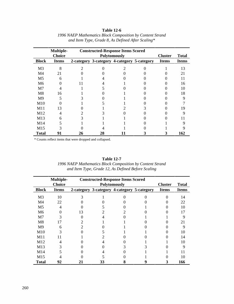
260

Table 12-61996 NAEP Mathematics Block Composition by Content Strand

and Item Type, Grade 8, As Defined After Scaling*

Multiple-Choice

Constructed-Response Items ScoredPolytomously Cluster Total

Block Items 2-category 3-category 4-category 5-category Items Items

M3 8 2 0 2 0 1 13M4 21 0 0 0 0 0 21M5 6 1 4 0 0 0 11M6 0 11 4 1 0 0 16M7 4 1 5 0 0 0 10M8 16 1 0 1 0 0 18M9 5 3 0 1 0 0 9

M10 0 1 5 1 0 0 7M11 13 0 1 2 3 0 19M12 4 2 3 0 0 0 9M13 6 3 1 1 0 0 11M14 5 1 1 1 0 1 9M15 3 0 4 1 0 1 9Total 91 26 28 11 3 3 162

* Counts reflect items that were dropped and collapsed.

Table 12-71996 NAEP Mathematics Block Composition by Content Strand

and Item Type, Grade 12, As Defined Before Scaling

Multiple-Choice

Constructed-Response Items ScoredPolytomously Cluster Total

Block Items 2-category 3-category 4-category 5-category Items Items

M3 10 3 1 0 0 0 14M4 22 0 0 0 0 0 22M5 4 0 5 0 1 0 10M6 0 13 2 2 0 0 17M7 3 0 4 0 1 1 9M8 17 2 1 1 0 0 21M9 6 2 0 1 0 0 9

M10 3 0 5 1 1 0 10M11 11 1 2 0 0 0 14M12 4 0 4 0 1 1 10M13 3 0 0 3 3 0 9M14 5 0 4 0 1 1 11M15 4 0 5 0 1 0 10Total 92 21 33 8 9 3 166

261

Table 12-81996 NAEP Mathematics Block Composition by Content Strand

and Item Type, Grade 12, As Defined After Scaling*

Multiple-Choice

Constructed-Response Items ScoredPolytomously Cluster Total

Block Items 2-category 3-category 4-category 5-category Items Items

M3 10 3 1 0 0 0 14M4 22 0 0 0 0 0 22M5 4 0 6 0 0 0 10M6 0 13 2 2 0 0 17M7 3 0 4 1 0 1 9M8 17 2 1 1 0 0 21M9 6 2 0 1 0 0 9

M10 3 0 5 2 0 0 10M11 11 1 2 0 0 0 14M12 4 0 4 1 0 1 10M13 3 0 0 4 2 0 9M14 4 1 3 1 0 1 10M15 4 1 5 0 0 0 10Total 91 23 33 13 2 3 165

* Counts reflect items that were dropped and collapsed.

12.3 SPECIAL MATHEMATICS ASSESSMENTS

There were three special studies in the 1996 NAEP assessment—estimation, theme, and advancedstudies. The block structure of the special study booklets is provided only in Table 12-9. The estimation andthe two theme blocks have a linking BIB block, M4, in the first position. This structure held for all threegrades, but the actual items in the blocks varied over grades. In addition to the cognitive blocks, each of thespecial study booklets included three blocks in common with the main assessment:

a general student background block (BM1), a mathematics background block (MB1), and a motivation block (M2).

Table 12-9Block Structure of the Special Study Booklets

Study Booklet Cognitive Blocks

Estimation 127 M4, M16, M17Theme 128 M4, M21Theme 129 M4, M22

Advanced Mathematics1 130 M20, M18, M191 Grades 8 and 12 only

262

The cognitive portion of the estimation booklet was administered in two sections: first there was a regularmathematics block in common with the main assessment that was self-paced; and second, there were twoestimation blocks (M16 and M17) in which items were administered by a paced audio tape. The theme andadvanced booklets were self-paced. Note that the theme booklets contained a single non-theme block (M4)in common with the main assessment.

The special studies were not part of the main assessment; analysis for these booklets will appearin separate focus reports. The major findings for these studies will be derived from an analysis of the‘reporting’ samples, which are subsamples of the assessment’s total sample. The nonreporting segmentsof the total samples were added to the assessments in order to study the effects of changing inclusionrules and accommodations for students of limited English proficiency (LEP) and students withdisabilities (SD) (See Section 12.4).

The estimation and theme samples were drawn from the same population as the main assessment.The grades 8 and 12 advanced booklets were drawn from a population of students considered to be highmathematics achievers. Students for the grade 8 study of advanced mathematics were sampled from apopulation of students who were enrolled in an advanced class (defined as algebra 1 or beyond) duringthe 1995-96 school year. For grade 12, the advanced study students were also sampled from a populationof students who took an advanced course during the school year. Grade 12 advanced courses were;Algebra 3, Pre-calculus, Calculus and Analytical Geometry, Calculus, and AP Calculus. Table 12-10 liststhe number of items in the special assessment blocks in the three grades. More detail is available in theprocedural appendices of reports on the estimation, theme and advanced analyses.

Table 12-10Number of Cognitive Items in the

1996 Special Mathematics Assessment Blocks

EstimationBlocks

ThemeBlocks

AdvancedBlocks

M16 M17 M21 M22 M20 M18 M19

Grade 4 20 14 8 6 —1 —1 —1

Grade 8 22 16 12 15 13 10 12 Grade 12 22 16 11 7 15 11 11

1 There were no advanced blocks administered to grade 4 students.

12.4 ASSESSING THE EFFECT OF CHANGING INCLUSION CRITERION ANDACCOMMODATIONS FOR SD/LEP STUDENTS

NAEP samples include SD/LEP students in at least the same percentages in which they are foundin the general school population. Although a substantial percentage of these students are included in theassessment, schools are allowed to exclude some of these students from NAEP when the students arejudged to be incapable of meaningfully participating in a large scale assessment. To facilitate theconsistent implementation of NAEP’s intention to include as many students as possible, NAEP providesspecific criteria that staff in sampled schools can use to determine who should be included in theassessment.

263

In the 1996 assessment, procedures for dealing with SD and LEP students were modified, basedon recommendations from the U.S. Department of Education. First, inclusion criteria were revised withthe intention of making them clearer, more inclusive, and more likely to be applied consistently acrossschools. Second, a variety of assessment accommodations and adaptations were offered to

students with disabilities whose individualized education programs (IEPs)specified such accommodations, and

LEP students who were unable to take the assessment in English. In order to assess the impact of new inclusion criteria and accommodations, a three-sampledesign was instituted at all three grades. The first sample comprised students who were subject to the1994 inclusion rules and, as was the case in past NAEP assessments, were offered no accommodations.Students in the second sample were subject to the 1996 inclusion rules but the SD/LEP students wereoffered no accommodations. The third sample had students who were comprised students who wereassessed under conditions that will probably be used for future NAEP assessments—new inclusion rulesand some accommodations being offered to the included SD/LEP students. See Chapter 3, Sections 3.4 to3.8, for more details. Results of this study can be found in the focus report dealing with the comparison of the threeaccommodation samples. 12.5 ITEM ANALYSIS This section contains a detailed description of the item analysis performed using the nationalmain BIB sample data. The analysis examines items within blocks. In preparation for this analysis,constructed-response items with more than two categories and cluster items were polytomously scored,two-category constructed-response items were dichotomously scored, and derived background variableswere calculated. Item statistics such as mean percent correct, average score, item to total scorecorrelations and percent responding in each item category were calculated. Tables 12-11, 12-12, and 12-13 show the number of items, mean proportion correct, mean item tototal score correlation, and alpha reliability for each block administered at each grade level for the mainassessment. These values were calculated within block only for those items used in the scaling process.The table also gives the number of students who were administered the block and the percent notreaching the last item in the block. Student weights were used, except for reporting the sample sizes. Theresults for the blocks administered at each grade level indicated that the blocks differ in number of items,average difficulty, reliability, and percent not reaching the last item. Tables 12-11 through 12-13 show the item analyses by block position within a booklet. Eachbooklet had three cognitive blocks, and each block appeared in three different booklets—once in the first,once in the second, and once in the third position. In some past assessments (e.g., 1992 science), studentsresponded differently to the items depending on the block position. The IA tables evidence fewsystematic differences in item summary statistics as a function of block position. For grade 4 (Table 12-11) the weighted average item score had a slight tendency to be higher when a block was in the firstrather than the third position. For grades 8 and 12 no systematic difference can be seen.

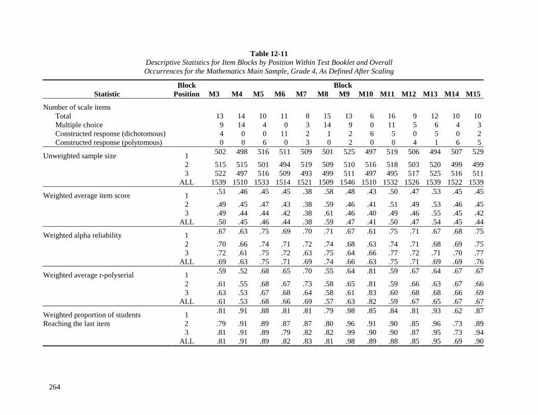
264

Table 12-11Descriptive Statistics for Item Blocks by Position Within Test Booklet and OverallOccurrences for the Mathematics Main Sample, Grade 4, As Defined After Scaling

Block BlockStatistic Position M3 M4 M5 M6 M7 M8 M9 M10 M11 M12 M13 M14 M15

Number of scale itemsTotal 13 14 10 11 8 15 13 6 16 9 12 10 10Multiple choice 9 14 4 0 3 14 9 0 11 5 6 4 3Constructed response (dichotomous) 4 0 0 11 2 1 2 6 5 0 5 0 2Constructed response (polytomous) 0 0 6 0 3 0 2 0 0 4 1 6 5

Unweighted sample size 1 502 498 516 511 509 501 525 497 519 506 494 507 529

2 515 515 501 494 519 509 510 516 518 503 520 499 4993 522 497 516 509 493 499 511 497 495 517 525 516 511

ALL 1539 1510 1533 1514 1521 1509 1546 1510 1532 1526 1539 1522 1539

Weighted average item score 1 .51 .46 .45 .45 .38 .58 .48 .43 .50 .47 .53 .45 .45

2 .49 .45 .47 .43 .38 .59 .46 .41 .51 .49 .53 .46 .453 .49 .44 .44 .42 .38 .61 .46 .40 .49 .46 .55 .45 .42

ALL .50 .45 .46 .44 .38 .59 .47 .41 .50 .47 .54 .45 .44

Weighted alpha reliability 1 .67 .63 .75 .69 .70 .71 .67 .61 .75 .71 .67 .68 .75

2 .70 .66 .74 .71 .72 .74 .68 .63 .74 .71 .68 .69 .753 .72 .61 .75 .72 .63 .75 .64 .66 .77 .72 .71 .70 .77

ALL .69 .63 .75 .71 .69 .74 .66 .63 .75 .71 .69 .69 .76

Weighted average r-polyserial 1 .59 .52 .68 .65 .70 .55 .64 .81 .59 .67 .64 .67 .67

2 .61 .55 .68 .67 .73 .58 .65 .81 .59 .66 .63 .67 .663 .63 .53 .67 .68 .64 .58 .61 .83 .60 .68 .68 .66 .69

ALL .61 .53 .68 .66 .69 .57 .63 .82 .59 .67 .65 .67 .67

Weighted proportion of students 1 .81 .91 .88 .81 .81 .79 .98 .85 .84 .81 .93 .62 .87

Reaching the last item 2 .79 .91 .89 .87 .87 .80 .96 .91 .90 .85 .96 .73 .893 .81 .91 .89 .79 .82 .82 .99 .90 .90 .87 .95 .73 .94

ALL .81 .91 .89 .82 .83 .81 .98 .89 .88 .85 .95 .69 .90

265

Table 12-12Descriptive Statistics for Item Blocks by Position Within Test Booklet and OverallOccurrences for the Mathematics Main Sample, Grade 8, As Defined After Scaling

Block BlockStatistic Position M3 M4 M5 M6 M7 M8 M9 M10 M11 M12 M13 M14 M15

Number of scale itemsTotal 17 21 12 16 10 18 9 7 19 9 11 14 12Multiple choice 12 21 7 0 4 16 5 0 13 4 6 10 6Constructed response (dichotomous) 3 0 1 16 1 2 3 7 6 2 4 1 0Constructed response (polytomous) 2 0 4 0 5 0 1 0 0 3 1 3 6

Unweighted sample size 1 558 556 543 571 555 541 546 543 538 547 543 550 539

2 535 558 548 556 561 566 542 534 551 530 544 546 5513 544 538 554 542 554 540 548 568 569 542 549 543 528

ALL 1637 1652 1645 1669 1670 1647 1636 1645 1658 1619 1636 1639 1618

Weighted average item score 1 .51 .58 .55 .59 .56 .50 .36 .56 .63 .34 .51 .41 .46

2 .50 .60 .54 .61 .56 .53 .35 .55 .65 .33 .51 .42 .453 .51 .58 .53 .62 .54 .50 .37 .55 .64 .34 .51 .41 .44

ALL .51 .59 .54 .61 .55 .51 .36 .55 .64 .34 .51 .41 .45

Weighted alpha reliability 1 .75 .76 .72 .82 .68 .79 .56 .65 .76 .60 .67 .58 .76

2 .75 .74 .70 .85 .66 .80 .63 .54 .79 .66 .68 .63 .723 .74 .78 .69 .82 .71 .76 .64 .58 .80 .68 .65 .64 .70

ALL .75 .76 .70 .83 .68 .79 .61 .59 .79 .64 .67 .61 .72

Weighted average r-polyserial 1 .66 .55 .63 .67 .66 .63 .58 .82 .62 .65 .62 .55 .70

2 .66 .53 .61 .73 .63 .63 .64 .76 .64 .68 .63 .56 .673 .66 .56 .61 .67 .70 .60 .64 .78 .65 .68 .62 .56 .65

ALL .66 .55 .62 .69 .66 .62 .62 .79 .64 .67 .62 .56 .67

Weighted proportion of students 1 .98 .87 .97 .90 .78 .72 .96 .90 .90 .81 .98 .76 .83

Reaching the last item 2 .93 .86 .96 .93 .76 .71 .94 .89 .87 .82 .96 .76 .853 .95 .88 .94 .92 .84 .75 .96 .92 .93 .85 .98 .80 .88

ALL .95 .87 .96 .91 .79 .72 .95 .90 .90 .83 .97 .77 .85

266

Table 12-13Descriptive Statistics for Item Blocks by Position Within Test Booklet and Overall

Occurrences for the Mathematics Main Sample, Grade 12, As Defined After Scaling

Block BlockStatistics Position M3 M4 M5 M6 M7 M8 M9 M10 M11 M12 M13 M14 M15

Number of scaled itemsTotal 14 22 10 17 9 21 9 10 14 10 9 14 10Multiple choice 10 22 4 0 3 17 6 3 11 4 3 8 4Constructed response (dichotomous) 4 0 0 17 0 4 2 6 3 0 5 1 1Constructed response (polytomous) 0 0 6 0 6 0 1 1 0 6 1 5 5

Unweighted sample size 1 525 530 519 536 539 548 530 526 523 540 532 526 516

2 515 519 539 523 525 529 545 547 524 516 536 544 5183 530 534 522 520 511 535 527 540 523 525 535 535 532

ALL 1570 1583 1580 1579 1576 1612 1602 1613 1570 1590 1603 1605 1566

Weighted average item score 1 .43 .70 .36 .55 .45 .55 .52 .47 .48 .41 .44 .47 .31

2 .43 .70 .37 .56 .43 .55 .49 .45 .51 .42 .41 .48 .313 .45 .70 .39 .56 .44 .56 .48 .43 .49 .41 .42 .48 .33

ALL .44 .70 .37 .56 .41 .55 .49 .45 .49 .40 .42 .48 .31

Weighted alpha reliability 1 .74 .76 .73 .83 .75 .80 .63 .52 .72 .70 .64 .76 .70

2 .69 .77 .71 .81 .74 .82 .59 .58 .69 .70 .66 .76 .703 .76 .75 .72 .81 .77 .80 .58 .62 .72 .68 .68 .80 .70

ALL .73 .76 .72 .82 .77 .81 .60 .58 .71 .76 .66 .78 .70

Weighted average r-polyserial 1 .69 .61 .72 .71 .70 .63 .65 .57 .63 .63 .67 .70 .72

2 .64 .61 .70 .68 .70 .63 .63 .61 .61 .60 .69 .69 .713 .70 .59 .70 .66 .73 .63 .60 .63 .63 .60 .70 .74 .69

ALL .68 .60 .71 .69 .74 .63 .63 .61 .63 .63 .69 .71 .71

Weighted proportion of students 1 .65 .84 .70 .78 .86 .48 .96 .88 .68 .78 .91 .78 .82

Reaching the last item 2 .67 .81 .70 .74 .86 .45 .94 .88 .70 .77 .90 .78 .813 .69 .78 .76 .65 .84 .50 .92 .87 .67 .83 .90 .77 .82

ALL .67 .81 .72 .72 .85 .48 .94 .88 .68 .79 .90 .78 .82

267

As described in Chapter 9, in NAEP analyses (both conventional and IRT-based), a distinction ismade between missing responses at the end of each block (not-reached) and missing responses prior tothe last completed response (omitted). Not-reached items are those occurring after the last item thestudent completed in a block. Items that were not reached are treated as if they had not been presented tothe examinee, while omitted items are regarded as incorrect. The proportion of students attempting thelast item of a block (or, equivalently, 1 minus the proportion not reaching the last item) is often used asan index of the degree of speededness of the block of items. Standard practice at ETS is to treat all students who did not respond to the last item as if they hadnot reached that item. For multiple-choice and short constructed-response items, this conventionproduced a reasonable pattern of results, in that the proportion of students reaching the last item does notdiffer markedly from the proportion attempting the next-to-last item. However, for the blocks that endedwith extended constructed-response items, this convention resulted in an implausibly large drop in thenumber of students attempting the final item (see Koretz et al., 1993). Therefore, for blocks that endedwith an extended constructed-response item, students who attempted the next-to-last item but did notrespond to the last item were classified as having intentionally omitted that item.

Tables 12-11 to 12-13 also contain information about the effect of the position of blocks withinbooklets on the average percent correct for items within each block presented to the BIB samples foreach grade. The averages for the grade-only portion of the focused-BIB samples show that the order ofblocks within booklets did not have a large or consistent effect on scale scores in the mathematicsfocused-BIB assessment.

12.5.1 Constructed-Response Items

As indicated in Tables 12-3 to 12-8, over 40 percent of the mathematics items were constructed-response. Constructed-response items that were scored dichotomously were given a right/wrong scoring.The categories of responses for the items and the number of responses that were rescored for each itemare indicated in Appendix I. The percent agreement for the raters and Cohen’s Kappa, a reliabilityestimate appropriate for items that are dichotomized, are also given in the tables. The sample sizes listedin the tables correspond to the samples used in calculating the rater reliability.

In general, the rater reliability of the scoring for dichotomized responses was quite high. Cohen’sKappa reliabilities ranged over items from 0.76 to 1.00 for grade 4, from 0.90 to 1.00 for grade 8, andfrom 0.67 to 1.00 for grade 12.

Chapter 7 discusses the definition of the item ratings and describes the process by which teamsof raters scored the constructed-response items. This discussion includes the rating definitions for shortand extended constructed-response items as well as the range of interrater reliabilities that occurred.Extended constructed-response items were scored on a scale from 1 to 5 to reflect degrees of knowledge.In scaling, this scale is shifted to 0 to 4. Rating information on extended constructed-response items canbe found in Appendix I, which lists the sample sizes, percent agreement, and Cohen’s Kappa reliabilityindex.

268

12.5.2 Differential Item Function Analysis

A differential item functioning (DIF) analysis of the main-assessment mathematics items wasdone in order to guide committees in identifying biased items that should be examined more closely forpossible bias. Sample sizes were large enough to compare male and female students, White and Blackstudents, and White and Hispanic students.

The DIF analyses of the dichotomous items were based on the Mantel-Haenszel chi-squareprocedure, as adapted by Holland and Thayer (1988), which is described in Chapter 9. The proceduretests the statistical hypothesis that the odds of correctly answering an item are the same for two groups ofexaminees that have been matched on some measure of mathematics ability (usually referred to as thematching criterion). The DIF analyses of the polytomous items were based on the Mantel procedure(1963) and the Somes (1986) chi-square test (see also Chapter 9). These procedures compare proportionsof matched examinees from each group in each polytomous item response category. The groups beingcompared are often referred to as the focal group (usually a minority or other group of interest, such asBlack examinees or female examinees) and the reference group (usually White examinees or maleexaminees).

For each dichotomous item in the assessment, an estimate was produced of the Mantel-Haenszelcommon-odds ratio, expressed on the ETS delta scale for item difficulty. The estimates indicate thedifference between reference group and focal group item difficulties (measured in ETS delta scale units),and typically run between about +3 and -3. Positive values indicate items that are differentially easier forthe focal group than the reference group after making an adjustment for the overall level of mathematicsability in the two groups. Similarly, negative values indicate items that are differentially harder for thefocal group than the reference group. It is common practice at ETS to categorize each item into one ofthree categories (Peterson, 1988): “A” (items exhibiting no DIF), “B” (items exhibiting a weak indicationof DIF), or “C” (items exhibiting a strong indication of DIF). Items in category “A” have Mantel-Haenszel common-odds ratios on the delta scale that do not differ significantly from 0 at the alpha = 0.05level or are less than 1.0 in absolute value. Category “C” items are those with Mantel-Haenszel valuesthat are significantly greater than 1 and larger than 1.5 in absolute magnitude. Other items are categorizedas B items. A plus sign (+) indicates that items are differentially easier for the focal group; a minus sign(- ) indicates that items are differentially more difficult for the focal group.

The ETS/NAEP DIF procedure for polytomous items incorporates both the MH ordinalprocedure and the generalized MH statistic. The summary tables of identified polytomous items containgeneralizations of the dichotomous “A,” “B,” and “C” categories namely “AA,” “BB,” and “CC”respectively. Analogous to the dichotomous case, only the “CC” items are considered to have a strongindication of DIF and are flagged for scrutiny by the subject matter committee

For each block of items at each grade four DIF comparisons were made: male/female,White/Asian American, White/Black, and White/Hispanic. The first subgroup in each comparison is thereference group; the second subgroup is the focal group.

Following standard practice at ETS for DIF analyses conducted on final test forms, all“C” and “CC” items were reviewed by a committee of trained test developers and subject-matterspecialists. As indicated by Tables 12-14 and 12-15, two dichotomous items and five polytomousitems met the criteria to be considered by the DIF committee. Such committees are charged withmaking judgments about whether or not the differential difficulty of an item is unfairly related togroup membership. See Appendix J for a list of the “C” and “CC” items.

269

The committee assembled to review NAEP items included both ETS staff and outside memberswith expertise in the field. It was the committee’s judgment that none of the “C” or “CC” items for thenational data were functioning differentially due to factors irrelevant to test objectives. In other words, allof the items that were classified as “C” or “CC” items measured concepts in the assessment frameworkand specifications that could not be measured in another way. Hence, none of the items were removedfrom scaling due to differential item functioning.

Table 12-14DIF Category by Grade for Dichotomous Items

DIF AnalysisGrade Category1 Male/Female White/Black White/Hispanic

4 C-B-A-A+B+C+

01

11710

029540

00

10910

8 C-B-A-A+B+C+

02

13900

007

1520

00

13830

12 C-B-A-A+B+C+

03

14500

018

1201

00

111001

1 Positive values of the index indicate items that are differentially easier for the focal group (female,Black, or Hispanic students) than for the reference groups (male or White students). “A+” or “A-”means no indication of DIF, “B+” means a weak indication of DIF in favor of the focal group, “B-“means a weak indication of DIF in favor of the reference group and “C+” or “C-” means a strongindication of DIF.

270

Table 12-15DIF Category by Grade for Polytomous Items

DIF AnalysisGrade Category1 Male/Female White/Black White/Hispanic

4 CC-BB-AA-AA+BB+CC+

01

131030

01

141110

00

121500

8 CC-BB-AA-AA+BB+CC+

00

101610

32

14710

12

131010

12 CC-BB-AA-AA+BB+CC+

029

1810

03

141021

01

151220

1 Positive values of the index indicate items that are differentially easier for the focal group (female,Black, or Hispanic students) than for the reference groups (male or White students). “A+” or “A-”means no indication of DIF, “B+” means a weak indication of DIF in favor of the focal group, “B-“means a weak indication of DIF in favor of the reference group and “C+” or “C-” means a strongindication of DIF.

12.5.3 Estimation of Item Parameters

The BILOG/PARSCALE computer program was used to estimate the item parameters for the mainassessment and for the special estimation study. For dichotomous multiple-choice and dichotomizedconstructed-response items, a three-parameter IRT model was used. Extended constructed-response andcluster items were polytomously scored and were analyzed with a generalized partial credit model (Muraki,1992).

Recall from section 12.5 that for calibration, items that were missing prior to the last completeditem in a block were considered omitted and scored as wrong. Also, items that were not reached weretreated as if they were not presented to the examinees (and not counted as wrong.) However, there is anexception for blocks that end with an extended constructed-response item. In these blocks, students whorespond to the next-to-last item but do not respond to the last item are classified as having omitted the lastitem (i.e., the last item is counted as wrong). Responses to extended constructed-response items that wereoff-task were also treated as omitted. The multi-category constructed-response items had two, three, four orfive categories of partial credit. Scoring levels were labeled as listed in Table 12-16.

271

Table 12-16Labels for Score Levels of Polytomous Items

Score 3-Category Item 4-Category Item 5-Category Item4 Correct3 Correct 4th Category2 Correct 3rd Category 3rd Category1 2nd Category 2nd Category 2nd Category0 Incorrect, off-task, or

omittedIncorrect, off-task, oromitted

Incorrect, off-task, oromitted

Note that the categories falling between “incorrect” and “correct” represent increasing levels of a partiallycorrect response.

The item parameter estimation was done separately within grade, but the final mathematics scaleestimates were transformed to conform with the cross-grade scales of the 1990 and 1992 assessments.Within each grade, items were scaled using the grade-only sample of students available from the 1992 andthe 1996 assessments. The 1992 data were included at the scaling step of the analysis to assure thatparameter estimates for items administered at both time points would not drift drastically betweenassessments. Item parameters were estimated separately for each of the five content strands and themathematics scale means and variances for samples from the two assessment years were allowed to bedifferent. In the final BILOG/PARSCALE run, the prior distributions of the population abilities were free tobe estimated and the overall distribution was centered at zero. In general, if an item was common to bothassessment years, identical item parameters were used for both assessments. The appropriateness of the useof the identical parameters across assessments was examined by comparing the fit of the empirical itemresponse functions against the estimated IRT item response functions. If IRT parameters did not fit the data,parameters specific to the assessment year were used. (See Chapter 11 for further descriptions of the scalingprocess.) The calibration was based on student weights that were rescaled so that the their sum equaled theunweighted sample size of the 1996 sample. Also, weights for the 1992 data were restandardized to giveequal weight to the two assessment years included in the scaling (see Appendix K).

Items that received special treatment in the scaling procedure are listed in Table 12-17, along withthe reason for special treatment. Items were dropped, combined into clusters, split between assessment yearsand collapsed. If items had empirical item response functions that were nonmonotonic, they were dropped.If several items had highly correlated responses (conditional on theta) they were combined into a singlepolytomous item called a cluster item. If items were administered in both 1992 and 1996 but showedevidence of having a distinct item response functions for each assessment year, the item is treated as twoseparate items and parameters estimated separately for each assessment year. If polytomous items hadsparse or nonmonotonic responses in one or more categories, the items were collapsed so that someresponse categories were combined into a single category. Only about ten percent of the total scaled itemswere given special treatment.

272

Table 12-17Items from the 1996 Assessment in Mathematics Receiving Special Treatment

GradeNAEP

ID BlockContentStrand Treatment

4 M010531 M8 1 1992 and 1996 responses split into itemsM010531Y and M010531Z

4 M040801 M9 2 1992 and 1996 responses split into itemsM040801Y and M040801Z

4 M041001 M9 2 1992 and 1996 responses split into itemsM041001Y and M041001Z

4 M041201 M9 3 1992 and 1996 responses split into itemsM041201Y and M041201ZCategories in both items collapsed: 0,1,2,3,4 becomes0,1,2,3,3,

4 M068001 M7 1 Collapsed categories: 0,1,2 becomes 0,0,1

4 M068003 M7 3 Collapsed categories: 0,1,2 becomes 0,0,1

4 M072701 M14 5 Collapsed categories: 0,1,2,3,4 becomes 0,1,2,3,3

4 M074701 M15 1 Collapsed categories: 0,1,2 becomes 0,0,1

8 M013531 M8 1 1992 and 1996 responses split into itemsM013531Y and M013531Z

8 M018201 M4 1 1992 and 1996 responses split into itemsM018201Y and M018201Z

8 M018901 M4 4 1992 and 1996 responses split into itemsM018901Y and M018901Z

8 M045901 1992 3 Collapsed categories: 0,1,2,3,4 becomes 0,1,2,3,31992 only

8 M050261 M3 4 Collapsed categories: 0,1,2,3,4 becomes 0,0,0,1,2

8 M051001 M3 3 1992 and 1996 responses split into itemsM051001Y and M051001Z

8 M051101 M3 1 1992 and 1996 responses split into itemsM051101Y and M051101ZCategories in both items collapsed: 0,1,2,3,4 becomes0,1,2,3,3

8 M051201 M13 1 1992 and 1996 responses split into itemsM051201Y and M051201Z

8 M052201 M13 2 Collapsed categories: 0,1,2,3,4 becomes 0,1,2,3,3

8 M053101 M9 4 Collapsed categories: 0,1,2,3,4 becomes 0,1,2,2,3

8 M054301 1992 5 Collapsed categories: 0,1,2,3,4 becomes 0,1,2,3,31992 only

273

Table 12-17 (continued)Items from the 1996 Assessment in Mathematics Receiving Special Treatment

GradeNAEP

ID BlockContentStrand Treatment

8 M055501 1992 1 Collapsed categories: 0,1,2,3,4 becomes 0,1,2,3,31992 only

8 M066301 M5 5 Collapsed categories: 0,1,2 becomes 0,1,1

8 M067501 M5 4 Collapsed categories: 0,1,2,3,4 becomes 0,1,2,2,2

8 M068201 M7 3 Collapsed categories: 0,1,2,3,4 becomes 0,0,1,1,1

8 M069301 M12 5 Collapsed categories: 0,1,2 becomes 0,1,1

8 M069601 M12 1 Collapsed categories: 0,1,2 becomes 0,1,1

8 M070001 M12 4 Collapsed categories: 0,1,2,3 becomes 0,1,2,2

8 M0732CL M14 4 Collapsed categories: 0,1,2,3,4 becomes 0,0,1,2,3

8 M073401 M14 1 Dropped due to bad item fit

8 M073501 M14 4 Collapsed categories: 0,1,2 becomes 0,1,1

8 M073601 M14 1 Collapsed categories: 0,1,2,3,4 becomes 0,1,2,3,3

8 M0757CL M15 5 Collapsed categories: 0,1,2,3 becomes 0,0,1,2

8 M076001 M15 2 Collapsed categories: 0,1,2,3,4 becomes 0,1,2,3,3

12 M073402 M14 1 Dropped

12 M025301 M5 1 Dropped 1992 only

12 M024901 M5 2 Dropped 1992 only

12 M070501,M070502

M12 4 Combined into cluster item M0705CL

12 M071701,M071702

M7 5 Combined into cluster item M0717CL

12 M071401 M5 1 Collapsed: 0,1,2,3,4 becomes 0,1,1,1,2

12 M056601 M3 1 1992 and 1996 responses split into itemsM056601Y and M056601Z

12 M062401 M10 3 1992 and 1996 responses split into itemsM062401Y and M062401ZBoth items collapsed: 0,1,2,3,4 becomes 0,1,2,3,3

12 M073901 M14 3 Collapsed categories: 0,1,2 becomes 0,1,1

12 M012731 M8 3 1992 and 1996 responses split into itemsM012731Y and M012731Z

12 M058701 M11 3 1992 and 1996 responses split into itemsM058701Y and M058791Z

12 M071801 M7 4 Collapsed categories: 0,1,2,3,4 becomes 0,1,1,2,3

274

Table 12-17 (continued)Items from the 1996 Assessment in Mathematics Receiving Special Treatment

GradeNAEP

ID BlockContentStrand Treatment

12 M070601 M12 4 Collapsed categories: 0,1,2,3,4 becomes 0,1,2,3,3

12 M0732CL M14 4 Collapsed categories: 0,1,2,3,4 becomes 0,0,1,2,3

12 M018901 M4 4 1992 and 1996 responses split into itemsM018901Y and M018901Z

12 M021501 M6 4 1992 and 1996 responses split into itemsM021501Y and M021501Z

12 M013131 M8 4 1992 and 1996 responses split into itemsM013131Y and M013131Z

12 M053401 M9 4 1992 and 1996 responses split into itemsM053401Y and M053401Z

12 M061905 M10 4 1992 and 1996 responses split into itemsM061905Y and M061905Z

12 M060701 M13 5 1992 and 1996 responses split into itemsM060701Y and M060701ZBoth items collapsed: 0,1,2,3,4 becomes 0,1,2,3,3

12 M074101 M14 5 Collapsed categories: 0,1,2,3,4 becomes 0,1,2,3,3

12 M077001 M15 5 Collapsed categories: 0,1,2,3,4 becomes 0,1,1,1,1

12 M021601 M6 5 1992 and 1996 responses split into itemsM021601Y and M021601Z

12 M021602 M6 5 1992 and 1996 responses split into itemsM021602Y and M021602Z

12.5.4 Evaluating the Fit of the IRT Model

During the course of estimating an IRT model, individual items were evaluated to determine howwell the item response model fit the data. This was done by visual inspection of plots comparingempirically based and theoretical item response functions. Specifically, for dichotomous items these plotsconsisted of nonmodel-based estimates of the expected proportion correct for each level of mathematicsability compared to the proportion correct for each level of mathematics ability as predicted by thetheoretical item response function. For polytomous extended constructed-response items, similar plotswere produced for each item category response function (see Chapter 9 for a fuller explanation of theseplots).

In making decisions about excluding items from the final scales, a balance was sought betweenbeing too stringent, hence deleting too many items and possibly damaging the content representativenessof the pool of scaled items, and being too lenient, hence including items with model fit poor enough toendanger the types of model-based inferences made from NAEP results. Items that clearly did not fit the

275

model were not included in the final scales; however, a certain degree of misfit was tolerated for anumber of items included in the final scales.

For most items, the model fit well. In a few cases, poor fit with the data led to special treatmentor deletion of the item. Figures 12-1, 12-4, 12-5 and 12-6 give item response plots of dichotomous items.In the plots, the x-axis depicts scale score, and the y-axis the probability of a correct response. The solidline is the logistic model prediction, and the symbols (usually a circle or diamond) are the nonmodel-based predicted proportions. The size of the symbols are proportional to the estimated number of studentsat a particular scale score level. The symbols are ordinarily larger in the middle of the theta scale, wheremost students’ scale scores fall. The item parameter values are also included in the plot.

Item response plots for polytomously scored items are given in Figures 12-2, 12-3, 12-7, and12-8. These are similar to the plots for dichotomous items except that there are several solid lines, one foreach item category, with each line indicating the probability of responding in the respective itemcategory. As before, the circles or diamonds indicate the empirical response function, with the size of thecircles and diamonds proportional to the estimated number of students at a scale score level.

In the plots good fit of the model to the data is indicated when the model-based functions (solidlines) coincide with the empirical functions (circles, diamonds, or other symbols).When the empiricalplot is far away from the model based line, there is poor fit of the model to the data.

Four examples of fit are illustrated. First there is good model fit which is shown by Figure 12-1for a dichotomous item and Figure 12-2 for a polytomous item. In both cases empirical and theoreticallines coincide.

Second is an example of an item that displayed non-logistic empirical functions and wasdropped. Figure 12-3 shows a polytomous item that was dropped from the assessment.

Third is an example of an item that changed function from one assess year to another. Figure 12-4 shows that the empirical item functions for two assessment years (diamonds for 1992 and circles for1996) are distinctly different. Figures 12-5 and 12-6 show the result of estimating item parametersseparately for the two years. This ‘splitting’ of the item across years results in quite good fit for eachyear.

The fourth example is of a poor fitting polytomous item that was modified by collapsingcategories. Figure 12-7 shows a 5-category item which evidences poor fit mostly in the upper category,due in large part to a low number of respondents. As a result, the upper two categories were collapsedresulting in a 4-category item which, as Figure 12-8 illustrates, fits satisfactorily.

276

Figure 12-1Dichotomous Item Exhibiting Good Model Fit*

*Circles (1996 data) and diamonds (1992 data) indicate estimated conditional probabilities obtained without assuming a logisticform; the solid curve indicates estimated item response function assuming a logistic form.

277

Figure 12-2Polytomous Item Exhibiting Good Model Fit*

a= 0.5634b= 0.6933d1= 1.9463d2= -0.3616d3= -1.0074d4= -0.5773fit= 3.55

a = 0.5634b = 0.6933d1 = 1.9463d2 = -0.3616d3 = -1.0074d4 = -0.5773

*Circles indicate estimated conditional probabilities obtained without assuming a model-based form; the solid curves indicateestimated item response function assuming a model-based form.

278

Figure 12-3Polytomous Item Exhibiting Bad Model Fit That

Was Deleted from the Assessment*

a= 0.6338b= 1.7533d1= 0.1185d2= -01185fit= 78.73

a = 0.6338b = 1.7533d1 = 0.1185d2 = -0.1185

*Circles indicate estimated conditional probabilities obtained without assuming a model-based form; the solid curves indicateestimated item response function assuming a model-based form.

279

Figure 12-4Dichotomous Item Exhibiting Different Empirical Item Functions for Different Assessment Years*

*Diamonds represent 1992 data; circles represent 1996 data. Circles and diamonds indicate estimated conditional probabilitiesobtained without assuming a logistic form; the solid curve indicates estimated item response function assuming a logistic form.

280

Figure 12-5Dichotomous Item Fit Separately to the 1992 Data and Exhibiting Good Model Fit*

*Diamonds indicate estimated conditional probabilities obtained without assuming a logistic form; the solid curve indicatesestimated item response function assuming a logistic form.

281

Figure 12-6Dichotomous Item Fit Separately to the 1996 Data and Exhibiting Good Model Fit*

*Circles indicate estimated conditional probabilities obtained without assuming a logistic form; the solid curve indicatesestimated item response function assuming a logistic form.

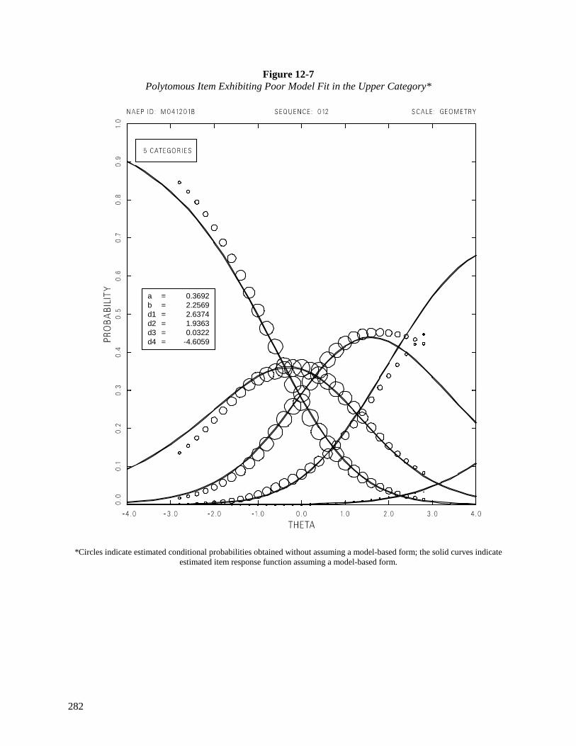
282

Figure 12-7Polytomous Item Exhibiting Poor Model Fit in the Upper Category*

a = 0.3692b = 2.2569d1 = 2.6374d2 = 1.9363d3 = 0.0322d4 = -4.6059

*Circles indicate estimated conditional probabilities obtained without assuming a model-based form; the solid curves indicateestimated item response function assuming a model-based form.

283

Figure 12-8Polytomous Item With the Upper Two Categories Collapsed, Now Exhibiting Good Model Fit*

a= 0.3824b= 0.6994d1= 1.0777d2= 0.3514d3= -1.4291fit= 3.15

a = 0.3824b = 0.6994d1 = 1.0777d2 = 0.3514d3 = -1.4291

*Circles indicate estimated conditional probabilities obtained without assuming a model-based form; the solid curves indicateestimated item response function assuming a model-based form.

12.5.5 Derived Background Variables

Derived variables are variables which use information from more than one background question.They were used for two purposes: as conditioning variables and as reporting variables used to definesubgroups. Some of these variables are common to all the subject areas; others are specific to the 1996mathematics assessment. Derived variables used for conditioning and reporting are described in Appendix C.

284

12.5.6 Generation of Plausible Values

For the entire sample, multivariate plausible values for content strand scales were generated foreach grade group separately using the multivariate conditioning program CGROUP as revised by Thomas(1993). As with the scaling, student weights were used at this stage of the analysis. Instead of using selectedbackground variables for conditioning variables (as had been done prior to the 1990 assessment), principalcomponents of the background variables were used. The principal components used accounted for 90percent of the variance of the original conditioning variables. Principal components were employed toremedy problems of extreme collinearity among some of the original conditioning variables.

Research based on data from the 1990 Trial State Assessment in mathematics suggests that resultsobtained using the 90 percent subset of components will differ only slightly from those obtained using thefull set (Mazzeo, Johnson, Bowker, & Fong, 1992). Table 12-18 lists the number of principal componentsincluded in conditioning, as well as the proportion of variance accounted for by the conditioning model foreach grade.

Table 12-18Proportion of Scale Score Variance Accounted for by the Conditioning Model

for the Mathematics Main Assessment

Proportion of Scale Score Variance

Grade

Number ofConditioning

Contrasts

Number ofPrincipal

Components

NumberSense,

Properties,and

Operations Measurement

Geometryand

SpatialSense

DataAnalysis,Statistics,

andProbability

Algebraand

Functions

4 895 321 .70 .71 .61 .75 .69

8 1,027 362 .71 .75 .68 .77 .73

12 812 314 .76 .79 .81 .70 .83

The codings of the original mathematics-specific conditioning variables, before principalcomponents were calculated, are presented in Appendix C. The CGROUP program estimates distributionsof scale scores by combining information from item responses of individuals and information from linearregression of scale score on conditioning variables. For each individual, five plausible values are randomlydrawn from their predictive conditional distribution.

The proportion of variance of each original conditioning variable accounted for by the principalcomponents included in the conditioning model is listed in Appendix F. The estimated conditioning effectsfor the principal components of the three samples defined by the three grade groups are also given inAppendix C. The values of the conditioning effects are expressed in the metrics of the original calibrationscale. Definitions of derived conditioning variables are given in Appendix B.

285

12.5.7 The Transformation of the Mathematics Calibration Scale for Reportingand the Formation of the Composite Scale

Like all IRT scales, the mathematics content strand scales have a linear indeterminacy that may beresolved by an arbitrary choice of the origin and unit-size in each given content strand. In 1990 the NAEPmathematics data were scaled across grades separately for each scale. The linear indeterminacies among thescales were resolved by transforming the scale means and variances of three grade samples combinedtogether to the 250.5 4, 50.0 metric using a transformation of the form,

θtarget = A • θcalibrated + B,

where A and B are linear transformation constants.

As a result, all of the scales that spanned all three grade samples were on a common scale. Bycontrast, the 1992 and 1996 data were scaled within grade. It was necessary, therefore, to transform datafrom both assessments to the 1990 cross-grade scale. This was accomplished first in the 1992 assessment,when the 1992 data were linked to the 1990 scale in a two-stage process. In the next assessment, the 1996data were linked to the 1992 transformed scale, which in effect put the 1996 data on the 1990 cross-gradescale. The procedure for transforming the 1996 data will be described below. The similar procedure fortransforming the 1992 data was presented in The NAEP 1992 Technical Report (Johnson and Carlson,1994).

The 1996 data were put on the 1992 reporting metric by using a linear transformation that convertsthe 1996 thetas to the 1992 reporting scale. This linear transformation was created by the followingprocedure. The 1992 thetas were reconditioned using CGROUP with the 1996 item parameters. Thisanalysis resulted in 1992 scores which were in the 1996 theta metric. We then transformed the new 1992thetas (in the 1996 metric) to the 1992 reporting metric (in the 1992 metric) by a linear transformationwhich created scores having the same mean and variance as the 1992 reporting scale. This is a commonpopulation equating procedure. The linear constants of this transformation were then used to transform the1996 thetas to the 1992 reporting metric. The transformation constants used for the five content strandscales and for the estimation scale are given in Table 12-19.

While scores in five content strands provide useful insights into the relationships amongsubpopulations, a single index to summarize overall performance is a useful tool for a compact overview ofsubpopulation trends. For that reason, a composite score was defined as a weighted average of the fivemathematics content strands. The weight given to each content strand is a direct reflection of the relativetesting time intended for that content strand in the assessment, as defined in the Mathematics Frameworkfor the 1996 National Assessment of Educational Progress (National Assessment Governing Board, 1994).Since the emphasis given to each content strand was different across grades, the weights assigned to eachstrand in the composite also differed across grades.

4 The function RPs = 250 + 50(θs) would have been preferable. Holland and Zwick (1986) have noted that the values actuallyused correspond to the bi varying from –5.00 to +4.98 in steps of .02 instead of –4.99 to +4.99 as intended. The result is that theRP scores are a half-point higher than appropriate for the hypothetical test.

286

Table 12-19Coefficients of the Linear Transformations that Transform the Five Content Strand Scales

from the 1996 Calibration Metric to the 1992 Reporting Metric

Grade Coefficient

Number Sense,Properties,

andOperations Measurement

Geometryand Spatial

Sense

Data Analysis,Statistics, and

ProbabilityAlgebra and

Functions

4 BA

220.3233.13

226.02 32.22

224.70 28.04

223.38 30.86

223.63 29.47

8 BA

273.44 35.12

269.33 43.65

266.83 33.54

270.97 41.00

271.13 35.52

12 BA

300.43 32.48

300.85 35.71

304.67 36.05

301.03 34.58

303.42 35.95

The definition of weights for the composite in each grade is given in Table 12-20. The mean andstandard deviations of the composite scales for all three grades is given in Table 12-21. Note that thiscomposite can be compared with the 1990 and 1992 composite scores since all three scales are on the 1990cross-grade scale (as defined in the beginning of this section).

Table 12-20Weights for the Mathematics Composite by Grade

Scale Grade 4 Grade 8 Grade 12

Number Sense, Properties, and Operations

Measurement

Geometry and Spatial Sense

Data Analysis, Statistics, and Probability

Algebra and Functions

.40

.20

.15

.10

.15

.25

.15

.20

.15

.25

.20

.15

.20

.20

.25

Table 12-21Means and Standard Deviations on the Mathematics Composite Scale

All Five Plausible ValuesGrade Mean S. D.

4 223.9 31.2

8 272.0 36.4

12 304.0 32.2

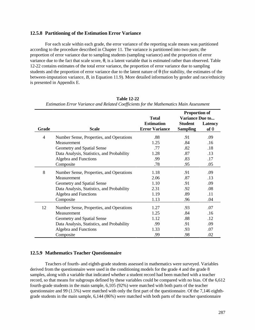
287

12.5.8 Partitioning of the Estimation Error Variance

For each scale within each grade, the error variance of the reporting scale means was partitionedaccording to the procedure described in Chapter 11. The variance is partitioned into two parts; theproportion of error variance due to sampling students (sampling variance) and the proportion of errorvariance due to the fact that scale score, θ, is a latent variable that is estimated rather than observed. Table12-22 contains estimates of the total error variance, the proportion of error variance due to samplingstudents and the proportion of error variance due to the latent nature of θ (for stability, the estimates of thebetween-imputation variance, B, in Equation 11.9). More detailed information by gender and race/ethnicityis presented in Appendix E.

Table 12-22Estimation Error Variance and Related Coefficients for the Mathematics Main Assessment

TotalProportion of

Variance Due to...

Grade ScaleEstimation

Error VarianceStudent

SamplingLatency

of θ

4 Number Sense, Properties, and OperationsMeasurementGeometry and Spatial SenseData Analysis, Statistics, and ProbabilityAlgebra and FunctionsComposite

.881.25.77

1.28.99.78

.91

.84

.82

.87

.83

.95

.09

.16

.18

.13

.17

.05

8 Number Sense, Properties, and OperationsMeasurementGeometry and Spatial SenseData Analysis, Statistics, and ProbabilityAlgebra and FunctionsComposite

1.182.061.102.311.191.13

.91

.87

.91

.92

.89

.96

.09

.13

.09

.08

.11

.04

12 Number Sense, Properties, and OperationsMeasurementGeometry and Spatial SenseData Analysis, Statistics, and ProbabilityAlgebra and FunctionsComposite

1.271.251.12.99

1.33.99

.93

.84

.88

.91

.93

.98

.07

.16

.12

.09

.07

.02

12.5.9 Mathematics Teacher Questionnaire

Teachers of fourth- and eighth-grade students assessed in mathematics were surveyed. Variablesderived from the questionnaire were used in the conditioning models for the grade 4 and the grade 8samples, along with a variable that indicated whether a student record had been matched with a teacherrecord, so that means for subgroups defined by these variables could be compared with no bias. Of the 6,612fourth-grade students in the main sample, 6,105 (92%) were matched with both parts of the teacherquestionnaire and 99 (1.5%) were matched with only the first part of the questionnaire. Of the 7,146 eighth-grade students in the main sample, 6,144 (86%) were matched with both parts of the teacher questionnaire

288

and 49 (less than 1%) were matched with only the first part of the questionnaire. Thus, 92 percent of thefourth graders and 86 percent of the eighth graders were matched with at least the background informationabout their mathematics teachers.

12.5.10 Analysis of Dimensionality

Plausible values are drawn from the set of five correlated content strands (see Section 12.5.6). For thisreason, it is useful to inspect the correlations among the content strands for evidence of multidimensionality.Tables 12-23 and 12-24 give conditional and marginal correlations for the five scales for the three grades.Conditional correlations are analogous to pooled-within groups correlations when the groups are the groupingvariables used to condition the data with CGROUP. They are obtained from the error correlations of aCGROUP analysis. The conditional correlations are quite high, averaging .85 for grade 4, .91 for grade 8, and.85 for grade 12. The marginal correlations are the average correlations of the five plausible values of eachscale. In this case they average .86 for grade 4, .88 for grade 8, and .87 for grade 12. Although it is ofsubstantive interest to analyze the scales separately, the correlations indicate that they are highly redundant.

Table 12-23Conditional Correlations from Conditioning (CGROUP)

Grade Scale

Number Sense,Properties,

andOperations Measurement

Geometryand

SpatialSense

Data Analysis,Statistics,

andProbability

Algebraand

Functions4 Number Sense, Properties, and

OperationsMeasurementGeometry and Spatial SenseData Analysis, Statistics, andProbabilityAlgebra and Functions

1.00 .89 .80

.96 .94

1.00 .78

.90 .85

1.00

.75 .78

1.00 .89 1.00

8 Number Sense, Properties, andOperationsMeasurementGeometry and Spatial SenseData Analysis, Statistics, andProbabilityAlgebra and Functions

1.00 .92 .79

.96 .97

1.00 .92

.95 .95

1.00

.86 .84

1.00 .96 1.00

12 Number Sense, Properties, andOperationsMeasurementGeometry and Spatial SenseData Analysis, Statistics, andProbabilityAlgebra and Functions

1.00 .96 .90

.84 .91

1.00 .94

.80 .89

1.00

.67 .88

1.00 .66 1.00

289

Table 12-24Marginal Correlations of Science Scales1

Grade Scale

Number Sense,Properties,

andOperations Measurement

Geometryand

SpatialSense

Data Analysis,Statistics,

andProbability

Algebraand

Functions4 Number Sense, Properties, and

OperationsMeasurementGeometry and Spatial SenseData Analysis, Statistics, andProbabilityAlgebra and Functions

1.00 .89 .84

.91 .92

1.00 .83

.86 .86

1.00

.81 .82

1.00 .86 1.00

8 Number Sense, Properties, andOperationsMeasurementGeometry and Spatial SenseData Analysis, Statistics, andProbabilityAlgebra and Functions

1.00 .89 .84

.91

.92

1.00 .89

.89 .89

1.00

.85 .86

1.00 .90 1.00

12 Number Sense, Properties, andOperationsMeasurementGeometry and Spatial SenseData Analysis, Statistics, andProbabilityAlgebra and Functions

1.00 .90 .90

.88 .90

1.00 .90

.86 .87

1.00

.81 .90

1.00 .80 1.00

1 Tabled values were obtained by computing a separate Pearson correlation coefficient for each plausible value, computing Fisher’s z-transformationfor each value, computing the average of the transformed values, and computing the inverse transformation of the average.