The Mystery of Missing Real Spillovers in Southern Africa · 2014-06-04 · THE MYSTERY OF MISSING...

I n t e r n a t I o n a l M o n e t a r y F u n d

African Department

The Mystery of Missing Real Spillovers in Southern Africa

Some Facts and Possible Explanations

Olivier Basdevant, Andrew Jonelis, Borislava Mircheva, and Slavi Slavov

14/03

© 2014 International Monetary Fund

Cataloging-in-Publication Data Joint Bank-Fund Library

The mystery of missing real spillovers in Southern Africa [electronic resource] : some facts and possible explanations / by Oliver Basdevant . . . [et al.]. – Washington, D.C. : International Monetary Fund, c2014. 1 online resource.

Includes bibliographical references. Description based on online resource; title from digital title page. ISBN: 978-1-48436-344-6

1. Economic development—South Africa—Econometric models. 2. Economic development—Swaziland—Econometric models. I. Basdevant, Olivier. II. International Monetary Fund.

HC905.M97 2014eb

Please send orders to: International Monetary Fund, Publication Services

P.O. Box 92780, Washington, DC 20090, U.S.A. Tel.: (202) 623-7430 Fax: (202) 623-7201

E-mail: [email protected] Internet: www.elibrary.imf.org

www.imfbookstore.org

Disclaimer: The views expressed in this book are those of the authors and should not be reported as or attributed to the International Monetary Fund, its Executive Board, or the governments of any of its member countries.

iii

Contents

Introduction 1

1. Here Be Spillovers: Overview of Institutional Arrangementsand Stylized Facts 5

2. Here Be Spillovers: An Illustration Using GIMF Simulations 9

Overview of the Model 9 Impact of a Negative Demand Shock in South Africa 11 Spillovers From Financial Stress in South Africa 12 Impact of a Negative Supply Shock in South Africa 12

3. Where Are They? The Mystery of Missing Real Spillovers:Overview and Update of Econometric Estimates 14

4. Whodunit and Why? 28

Trade Linkages 28 Foreign Direct Investment and Financial Sector Linkages 30 Institutional Linkages 31

Conclusion 32

References 33

Figures

Figure 1. Real GDP Growth in Southern Africa, 1986–2012 1 Figure 2. South Africa’s Real GDP Growth, 1980–2018 3 Figure 3. Southern African Customs Union Receipts and South Africa’s

Imports 6 Figure 4. Net Migration in Southern Africa 7 Figure 5. Impact of a Negative Demand Shock in South Africa on Real

GDP in Swaziland 12 Figure 6. Impact of Financial Stress in South Africa on Real GDP

in Swaziland 12 Figure 7. Impact of a Negative Supply Shock in South Africa on Real

GDP in Swaziland 13 Figure 8. A Flowchart Summarizing the Economic Linkages between

South Africa and the Region 29

CONTENTS

iv

Tables

Table 1. Trade and Financial Linkages of Neighbor Countries with South Africa 2

Table 2. List of Parameter Values Used for the Calibration of the GIMF Model 11

Table 3. Impact of Growth in South Africa on Growth in Sub-Saharan Africa (Pooled panel, 1960–2009) 16



Table 6. Impact of Growth in South Africa on Growth in Sub-Saharan Africa (Fixed effects, 1960–2009) 20



Table 9. Impact of Growth in South Africa on Growth in Sub-Saharan Africa (Interactions with neighbor dummy, pooled panel, 1960–2009) 23

Table 10. Impact of Growth in South Africa on Growth in Sub-Saharan Africa (2SLS, 1960–2009) 25



1

Introduction

South Africa has strong ties with other countries in the region, particularly with its neighbors—Botswana, Lesotho, Mozambique, Namibia, Swaziland, and Zimbabwe (henceforth, BLMNSZ). South Africa’s economy is by far the largest in the region. It accounts for about 85 to 90 percent of these seven countries’ total GDP at market exchange rates. It is often described as an “engine of growth” for the region. Thus, it is reasonable to expect that South Africa’s business cycle and its long-term growth rate will affect those of neighboring countries. However, Figure 1 and the associated

Figure 1 . Real GDP Growth in Southern Africa, 1986–2012 (Percent change, year-over-year)

–20.0

–15.0

–10.0

–5.0

0.0

5.0

10.0

15.0

20.0

25.0

86 88 90 92 94 96 982000 02 04 06 08 10 12

Botswana

Lesotho

Mozambique

Namibia

Swaziland

ZimbabweSouth Africa

Source: IMF, International Financial Statistics and African Department databases.

For constructive comments and ideas, we are grateful to Emre Alper, Alfredo Cuevas, Domenico Fanizza, Sebnem Kalemli-Ozcan, Dirk Muir, as well as our colleagues in the Southern II division of the IMF’s African Department. We are particularly indebted to Lamin Leigh and Laura Papi for their overall guidance and support.

THE MYSTERY OF MISSING REAL SPILLOVERS IN SOUTHERN AFRICA

2

Table 1 . Trade and Financial Linkages of Neighbor Countries with South Africa

Botswana Lesotho Mozambique Namibia Swaziland Zimbabwe

Correlation with SA’s GDP growth rate(contemporaneous, 1986–2012)

0.18 0.16 0.43 0.24 0.20 0.24

Correlation with SA’s GDP growth rate(5-year averages, 1986–2012)

0.37 0.54 0.72 0.20 0.48 0.75

Exports to South Africa(% of total exports, 2010)

13.2 38.9 21.4 31.4 58.2 55.4

Exports to South Africa(% of GDP, 2010)

4.1 15.3 4.7 11.0 27.4 18.8

Imports from South Africa(% of total imports, 2010)

86.3 93.7 41.6 71.0 96.5 48.1

Imports from South Africa(% of GDP, 2010)

27.7 78.1 12.8 31.4 56.8 29.9

Exports of commodities(% of total goods exports)

93.11 n.a. 43.32 77.31 90.13 68.61

Exports of manufactured goods(% of total goods exports)

6.91 n.a. 56.72 22.71 9.93 31.41

Stocks of SA FDI(% of destination country GDP, 2010)

3.3 2.7 12.3 4.3 11.1 12.4

Stocks of FDI in SA(% of source country GDP, 2011)

1.9 2.8 n.a. 3.8 12.2 n.a.

Deposits in SA(% of source country GDP, 2010)

n.a. 20.0 1.3 3.3 9.7 1.1

Market share of SA banks(% of deposits, 2010)StanbicABSANedbankFirst Rand

1600+

+0

30+

20073

+7++

430

2321

140+0

Sources: Canales-Kriljenko, Gwenhamo, and Thomas (2013); IMF (2012), International Financial Statistics and African Department databases; South African Reserve Bank; and ZIMSTAT . Notes: FDI = foreign direct investment; n.a. = not available; SA = South Africa. 1 Based on 2001–12 trade data. 2 Based on 2001–11 trade data. 3 Based on 2005–12 trade data.

correlation coeffi cients in Table 1 show that there has been little or no correlation among GDP growth rates in Southern Africa in the past three decades. Mozambique is the only country whose GDP growth rate has been positively and signifi cantly correlated with South Africa’s (looking at either contemporaneous growth rates or at fi ve-year moving averages).

Introduction

3

Recent data suggest a slowdown in South Africa’s economy, which is projected to persist by private-sector analysts as well as by the IMF’s October 2013 World Economic Outlook . Figure 2 compares the latest projections for South Africa’s growth rate to those in the October 2012 World Economic Outlook . It also offers a long-term perspective on South Africa’s growth rate. It is apparent that in addition to a weaker cyclical recovery, the projections have taken a more conservative view of the country’s long-term growth prospects, with the growth rate of potential GDP revised downwards by a percentage point, to around 3 percent. A weaker cyclical recovery is projected because recent data suggest softer consumption and private investment. Regarding South Africa’s long-term growth prospects, the more pessimistic projections are driven by slow progress on the structural reform agenda and by delays in implementing the public infrastructure program (aimed at easing electricity and transportation bottlenecks). The lower potential growth in South Africa appears to be part of a broader trend among emerging markets following the global fi nancial crisis, which has been extensively documented in IMF (2013).

This paper studies the potential spillovers, both cyclical and long-term, from a slowdown in South Africa’s economy to the other economies in the region and beyond. Multiple linkages exist between South Africa’s economy and those of its neighbors. South Africa forms the Common Monetary Area together with Lesotho, Namibia, and Swaziland, with the rand serving as legal tender throughout and Lesotho, Namibia, and Swaziland currencies pegged

Figure 2 . South Africa’s Real GDP Growth, 1980–2018(Percent change, year-over-year)

–3.0

–2.0

–1.0

0.0

1.0

2.0

3.0

4.0

5.0

6.0

7.0

8.0

9.0

1980 82 84 86 88 90 92 94 96 982000 02 04 06 08 10 12 14 16 18

October 2012 WEO October 2013 WEOAverage 1980s Average 1990sAverage 2000s Average 2010s (October 2012 WEO)Average 2010s (October 2013 WEO)

Source: IMF, International Financial Statistics and World Economic Outlook databases. Note: WEO = World Economic Outlook .


4

to the rand at parity. There are strong fi scal channels at work in the region as well, due to the customs revenue-sharing mechanism under the Southern African Customs Union (SACU). South Africa is a key export destination for most countries in the region, and an even more important source of imports. It is also an important source of foreign direct investment (FDI). The branches and subsidiaries of South Africa–based banks dominate the banking sector in all neighboring countries. South African fi nancial and nonfi nancial fi rms also have a strong presence, while households and fi rms in the neighboring countries own fi nancial assets in South Africa. South Africa is home to an estimated almost two million workers from elsewhere in the Southern African Development Community (SADC), or just under 1 percent of SADC’s total population (excluding South Africa). The associated fl ows of remittances are signifi cant. Given all these linkages, it is logical to expect that South Africa’s GDP growth rate should affect those of its neighbors. In other words, there should be real spillovers.

This is an important research question. The IMF has made spillovers a priority in its surveillance of member countries. Existing studies of spillovers in Southern Africa have reached seemingly contradictory conclusions. While Arora and Vamvakidis (2005) found statistical evidence of real spillovers, Kabundi and Loots (2007), IMF (2012), and Canales-Kriljenko, Gwenhamo, and Thomas (2013) found no strong evidence of real spillovers from economic developments in South Africa to the region and the continent.

Chapter 1 reviews the institutional arrangements and stylized facts that would lead us to expect a high degree of real spillovers from South Africa to the region. Chapter 2 illustrates this point by numerically simulating the channels of transmission for Swaziland using a calibrated dynamic stochastic general equilibrium model (the IMF’s Global Integrated Monetary and Fiscal [GIMF] model). Swaziland was chosen for this exercise as it is a good example of the relationship between a small open economy in the region and South Africa. Chapter 3 reviews and updates the available econometric evidence and concludes that after 1994 there is no strong evidence of real spillovers from economic developments in South Africa, either cyclical or structural, to the region and the continent after controlling for global growth.

Chapter 4 investigates a number of plausible explanations for this surprising and counterintuitive fi nding. First, the extent of trade, fi nancial, and institutional integration in Southern Africa might be more limited than conventional wisdom and anecdotal evidence suggest. Second, as international sanctions ended and South Africa reintegrated with the world economy, the impact of South Africa’s growth on the region and the continent is no longer detectable separately from that of world growth. Finally, the multiple spillover channels might operate in ways that offset each other, so that their net impact is relatively small.

5

CHAPTER

Here Be Spillovers: Overview of Institutional Arrangements and Stylized Facts

Multiple linkages exist between South Africa’s economy and those of its neighbors. Starting with institutional ties, South Africa, Lesotho, Namibia, and Swaziland form the Common Monetary Area, with the rand serving as legal tender throughout and Lesotho, Namibia, and Swaziland currencies pegged to the rand at parity. The Botswana pula is linked to a currency basket that has a weight of around 55 percent on the rand, with the remaining 45 percent going to Special Drawing Rights . 1 Given highly integrated fi nancial markets and the wide circulation of the rand, Botswana, Lesotho, Namibia, and Swaziland (henceforth, BLNS) effectively import their monetary and exchange rate policy from South Africa. Tighter monetary conditions in South Africa immediately translate into tighter monetary conditions in BLNS countries, and should result in positively correlated business cycles.

Another important institutional linkage is provided by the customs revenue-sharing mechanism under SACU, which links closely South African import levels to BLNS fi scal positions. South Africa generates about half of SACU revenues. Therefore, customs revenues depend heavily on South African imports, which are procyclical. In turn, that makes SACU receipts for BLNS countries heavily dependent on South Africa’s business cycle. SACU revenues account for a substantial amount of fi scal revenues in all BLNS countries: over 20 percent of GDP for the smallest SACU members (Lesotho and Swaziland) and 12 to 13 percent of GDP for Botswana and Namibia in 2012 ( Figure 3 ). In the event of an adverse shock to South Africa, SACU transfers to BLNS countries may decrease sharply. In other words, the revenue-sharing formula propagates the negative shock in South Africa to the region.

1

1 Botswana’s monetary authorities also monitor the country’s real effective exchange rate as a guide to exchange rate policy.


6

South Africa is an important trade partner for its neighbors ( Table 1 ). Therefore, a slowdown in South African import demand could have a substantial effect on other countries’ exports, at least in theory. While South Africa accounted for only 13 percent of Botswana’s exports in 2010, that number ranges from 21 percent in Mozambique to 58 percent for Swaziland, with the other countries falling in between. South Africa is even more important as a source of imports for its neighbors, with import shares ranging from 42 percent in Mozambique to 96 percent in Swaziland in 2010. Given that neighbor countries are highly dependent on inputs and intermediate goods from South Africa (electricity, in particular), any supply disruptions or shortages (for example, due to strikes or worsening capacity constraints in South Africa) would have a negative impact on production and exports in neighboring countries.

South Africa is a key source of direct investment for its neighbors. According to Bank for International Settlements data summarized in Table 1 , the stock of South African foreign direct investments range from 3 to 4 percent of the recipient’s country GDP in Botswana, Lesotho, and Namibia to 11 to 12 percent of GDP in Mozambique, Swaziland, and Zimbabwe. In addition, South African nonfi nancial companies (such as large-scale retailers, mining companies, and manufacturers) have a signifi cant presence in the region. South Africa–based banks dominate the banking sector in all neighboring countries ( Table 1 ). If a growth slowdown in South Africa weakens the

Figure 3 . Southern African Customs Union Receipts and South Africa’s Imports (Percent of GDP)

0

5

10

15

20

25

30

35

40

45

2000 01 02 03 04 05 06 07 08 09 10 11 12

Lesotho’s receiptsNamibia’s receiptsSwaziland’s receiptsBotswana’s receiptsSouth Africa’s imports

Source: Country authorities.

Here Be Spillovers: Overview of Institutional Arrangements and Stylized Facts

7

balance sheets of South African fi rms, fi nancial or nonfi nancial, their weakness might propagate the slowdown to the rest of the region.

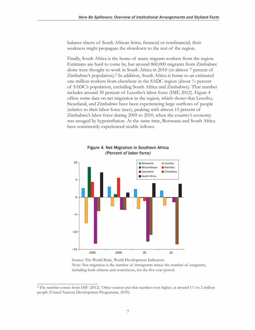
Finally, South Africa is the home of many migrant workers from the region. Estimates are hard to come by, but around 860,000 migrants from Zimbabwe alone were thought to work in South Africa in 2010 (or almost 7 percent of Zimbabwe’s population). 2 In addition, South Africa is home to an estimated one million workers from elsewhere in the SADC region (about ½ percent of SADC’s population, excluding South Africa and Zimbabwe). That number includes around 30 percent of Lesotho’s labor force (IMF, 2012). Figure 4 offers some data on net migration in the region, which shows that Lesotho, Swaziland, and Zimbabwe have been experiencing large outfl ows of people (relative to their labor force sizes), peaking with almost 15 percent of Zimbabwe’s labor force during 2005 to 2010, when the country’s economy was ravaged by hyperinfl ation. At the same time, Botswana and South Africa have consistently experienced sizable infl ows.

Figure 4 . Net Migration in Southern Africa (Percent of labor force)

–15

–10

–5

0

5

10

1995 2000 1005

Botswana LesothoMozambique NamibiaSwaziland ZimbabweSouth Africa

Source: The World Bank, World Development Indicators. Note: Net migration is the number of immigrants minus the number of emigrants, including both citizens and noncitizens, for the five-year period.

2 The number comes from IMF (2012). Other sources put that number even higher, at around 1½ to 2 million people (United Nations Development Programme, 2010).


8

Data on remittances are also patchy, as most remittance fl ows are informal and diffi cult to capture. IMF (2012) cites World Bank estimates according to which Lesotho’s remittances equaled 21 percent of GDP in 2010, while for Swaziland the amount was 3 percent. Several sources, including the United Nations Development Programme (2010), estimate Zimbabwe’s remittances at around 10 percent of GDP, while Botswana’s net private remittances are actually negative.

A slowdown in the South African economy would reduce its demand for labor, which would have a negative impact on remittances. A decline in remittances from South Africa would affect most neighboring countries negatively, with the strongest impact on the poor and vulnerable, who are most dependent on these transfers. In addition, increased joblessness in South Africa might force migrant workers to return to their home countries. If migrant workers are not easily re-absorbed into the domestic labor market (as is likely to be the case, given high unemployment rates throughout the region), then a large-scale return of migrant workers might cause social tensions and exert pressure on the budget.

9

CHAPTER

Here Be Spillovers: An Illustration Using GIMF Simulations

This section uses the IMF’s GIMF model to illustrate more formally how the channels described in the previous section would generate signifi cant spillovers. GIMF is suitable to analyze spillover effects because of its dynamic stochastic general equilibrium structure. Swaziland is chosen for this exercise as it is a good example of the relationship between a small open economy in the region and South Africa. The model links the two countries through bilateral trade and fi nancial fl ows. It explicitly models relative prices, including the real interest rate and the real exchange rate.

There are no other countries in the model; that is, it is a two-country world. The two-country assumption is due to the technical diffi culties associated with a three-country model, involving one very large economic area (the rest of the world) and two very small ones (South Africa and a neighbor). 3 Such a model would be diffi cult to simulate, since numerically accurate results would be feasible only with strong restrictions on the types of shocks under consideration. The two-country assumption limits somewhat the policy relevance of the model: while we can still use it to analyze the impact of shocks originating in South Africa on Swaziland, it is obviously not fi t to handle the impact of global shocks on either country or the role that South Africa plays as a conduit of global shocks for its smaller neighbors.

Overview of the Model 4

The version of the GIMF model we employ is a two-country model where all parameters except population growth and technology growth

2

3 South Africa produces ½ percent of global GDP, while Swaziland produces 0.005 percent. 4 See Kumhof and others (2010) for a more general and detailed presentation of GIMF.


10

can differ across countries. Both countries are populated by two types of households: overlapping generations (OLG) households and liquidity-constrained households. Both types of households consume fi nal retailed output, supply labor to labor unions, and are subject to uniform labor income, consumption, and lump-sum taxes. Firms are managed by myopic OLG households and therefore also have fi nite planning horizons. Given these modeling assumptions, Ricardian equivalence will not hold. Each country’s primary production is carried out by manufacturers producing tradable and nontradable goods. Manufacturers buy raw materials from the world market, labor from monopolistically competitive labor unions, and capital goods from their producers or from entrepreneurs. Manufacturers are subject to nominal rigidities in price setting as well as real rigidities in hiring labor and in using raw materials. Entrepreneurs fi nance their capital holdings using a combination of external and internal fi nancing. Monopolistically competitive retailers face real, instead of nominal, rigidities. The world economy experiences a constant positive growth rate of technology.

In addition, the model assumes that asset markets are incomplete. There is complete home bias in government debt, which takes the form of nominal noncontingent one-period bonds denominated in the domestic currency. The only assets traded internationally are pure consumption bonds that the households of the two countries buy and sell with each other. There is also complete home bias in the ownership of domestic fi rms. Furthermore, while households receive lump-sum dividend payments, equity is not traded in domestic fi nancial markets.

The model is calibrated to two countries: South Africa and Swaziland. The time unit of the model is one year. Swaziland is assumed to comprise ½ percent of world GDP. South Africa represents the “rest of the world” and comprises 99½ percent of world GDP. Both countries have a steady state infl ation rate of 2 percent per year. In the steady state, the world’s real GDP growth rate is assumed to be 1½ percent per year. World population is assumed to grow at 1 percent per year. The world real interest rate is assumed to be 3 percent per year. Households in both Swaziland and South Africa are assumed to have a planning horizon of 20 years. In addition, 70 percent of households in Swaziland and South Africa are assumed to be liquidity constrained, with the remaining 30 percent being myopic OLG households. Trade shares are calibrated based on 2011 data, while tax rates are calibrated based on 2007 data. In addition, the depreciation rates of public and private capital are set at 4 and 10 percent per year, respectively. Additional calibration values are presented in Table 2 . To the extent possible, these values have been selected based on country-specifi c data for South Africa and Swaziland.


11

Table 2 . List of Parameter Values Used for the Calibration of the GIMF Model(Percent, unless otherwise indicated)

Swaziland South Africa

Share of labor income in . . .Total economy 60 54Nontradable sector 66 60

Share of investment (% of GDP) 13.5 20Exports of final goods (% of GDP) 34.2 0.11Exports of intermediate goods (% of GDP) 12.08 0.11Imports of final goods (% of GDP) 34.21 0.17Fiscal parameters

Government consumption (% of GDP) 11 12Government investment (% of GDP) 3 4Tax revenue (% of GDP) 15.7 25.7Government debt (% of GDP) 8.4 35Share in total revenue of

Consumption tax revenue 9.9 9.3Capital tax revenue 3.5 3.7Labor tax revenue 6 12.9

Household parameters

Share of liquidity-constrained consumers 70 70Population growth rate 1 1Share of world population 1.74 98.26Habit persistence 0.4 0.4Probability of surviving (20-year planning horizon) 20 20Income decline rate (20-year remaining working life) 20 20Inverse of the intertemporal elasticity of substitution 2 2

Impact of a Negative Demand Shock in South Africa

The impact from a demand shock in South Africa on Swaziland’s real GDP is substantial. We simulated a temporary one-year decrease of aggregate demand in South Africa, driven by temporary autonomous decreases in both investment and consumption. This results in a 4 percent decline in South Africa’s real GDP in the short run, relative to trend. The contraction of South African demand affects negatively demand for Swaziland’s exports. Subsequently, Swaziland’s investment falls. As shown in Figure 5 , the real spillovers to Swaziland are positive and substantial: a slowdown in aggregate demand in South Africa results in a negative dip in Swaziland’s real GDP of over 2 percent, after which the economy gradually recovers. In other words, we could say that the spillover “elasticity” in Swaziland with respect to South Africa is about 0.5.


12

Spillovers From Financial Stress in South Africa

Another potential source of spillovers is fi nancial interconnectedness. More specifi cally, a temporary but persistent increase in borrowers’ riskiness in South Africa leads to an investment slowdown in the country. South Africa’s real GDP drops by close to 1½ percent over one year. Considering that the majority of banks in Swaziland are South African subsidiaries or branches, the shock in South Africa is combined with a similar one in Swaziland as well. This leads to a decrease in investment in Swaziland, which in turn has a negative effect on Swaziland’s real GDP. This effect is slightly above 1 percent, relative to trend (see Figure 6 ).

Impact of a Negative Supply Shock in South Africa

Finally, we analyzed a supply shock, which is another plausible channel of real spillovers from South Africa. A permanent decrease of 2½ percent in

Figure 5 . Impact of a Negative Demand Shock in South Africa on Real GDP in Swaziland

–2.5

–2

–1.5

–1

–0.5

0

0.5

1

1.5

0 1 2 3 4 5 6 7 8 9 10 11 12

Real GDP (% difference vs. steady-state)

Figure 6 . Impact of Financial Stress in South Africa on Real GDP in Swaziland

–1.5

–1

–0.5

0

0.5

1

1.5

0 1 2 3 4 5 6 7 8 9 10 11 12

Real GDP (% difference vs. steady-state)


13

the growth rate of productivity in South Africa affects negatively Swaziland’s real GDP by about 2½ percent (see Figure 7 ). The negative effect on both countries is permanent, as productivity growth in South Africa does not recover. The spillover elasticity under this scenario is close to one.

In conclusion, using a battery of real and fi nancial shocks, our numerical simulations show that negative shocks in South Africa typically spill over to Swaziland and cause cyclical downturns. In other words, we would expect to fi nd a positive correlation between South Africa’s business cycle and the business cycles of neighboring countries. These results formally illustrate our discussion in Chapter 1 .

Figure 7 . Impact of a Negative Supply Shock in South Africa on Real GDP in Swaziland

–3

–2.5

–2

–1.5

–1

–0.5

0

0 1 2 3 4 5 6 7 8 9 10 11 12

0.5 Real GDP (% difference vs. steady-state)

14

CHAPTERCHAPTER Where Are They? The Mystery of Missing Real Spillovers: Overview and Update of Econometric Estimates

Real spillovers from economic developments in South Africa to the rest of Southern Africa and the continent have been analyzed in Canales-Kriljenko, Gwenhamo, and Thomas (2013), IMF (2012), Kabundi and Loots (2007), and Arora and Vamvakidis (2005). In the following paragraphs, we provide an overview of their methodologies and results. In summarizing the results, it is useful to keep in mind the distinction between long-term trends and cyclical fl uctuations around those trends. We then discuss the results from our own econometric estimations, which replicate the methodology in Arora and Vamvakidis (2005) on a longer sample.

Kabundi and Loots (2007) discuss the co-movement between South Africa’s business cycle and those of other countries in the SADC region. The study uses annual data for 1980 to 2002 and a Generalized Dynamic Factor model. The model decomposes each country’s GDP growth rate into a common component and an idiosyncratic component. The model fi nds a high degree of correlation between South Africa’s common component and the common components of BLMNSZ countries (with correlation coeffi cients ranging from 0.59 to 0.99). However, it would seem that such high correlations would be there almost by construction. The common component of each country’s GDP would, by defi nition, be highly correlated with the common components of all other countries. In addition, the driving factor behind those high correlations among common components could be global shocks, in addition to genuine spillovers of South Africa–specifi c shocks to the region. The paper computes the percentage of the variance of each country’s growth rate explained by common components—a sort of R -squared. This percentage is rather low for BLMNSZ (0.08 to 0.25), implying that the common components do not have much explanatory power. In other words, idiosyncratic components explain most of the variance in GDP growth rates for South Africa’s neighbor countries.

Spillovers of cyclical shocks from South Africa to the rest of the continent are further studied in IMF (2012) and in Canales-Kriljenko, Gwenhamo, and

3

Where Are They? The Mystery of Missing Real Spillovers

15

Thomas (2013), with the latter focusing on BLNS. These papers list multiple economic linkages that appear signifi cant. However, formal econometric analysis fi nds their net impact to be statistically insignifi cant. Specifi cally, the two studies fi nd that contemporaneous correlation coeffi cients are rather modest—these are replicated in Table 1 for 1986 to 2012 and range from 0.43 in Mozambique to −0.24 in Zimbabwe. The two studies also employ dynamic panel regressions and vector autoregression models to conclude that cyclical fl uctuations in South Africa’s GDP do not seem to signifi cantly affect those in the Southern African Customs Union region or the rest of the continent, once the authors control for global shocks.

Arora and Vamvakidis (2005) fi nd positive and statistically signifi cant spillovers in long-term growth rates. Specifi cally, using standard panel growth regressions, the authors conclude that a 1 percentage point increase in South Africa’s long-term growth rate is associated with a ½ to ¾ percent increase in long-term growth rates in the rest of sub-Saharan Africa. This effect is large, especially considering that the authors already control for global and continent-wide factors. In addition, most of their sample (1960 to 1999) covers the era before 1994, when South Africa was a lot less integrated with the rest of the world, due to the apartheid system and international sanctions. One would have expected countries that are closer to South Africa or trade a lot with South Africa to have stronger growth spillovers. However, the authors show that this is not the case: neither geographical proximity nor greater trade in goods explain the correlation between South Africa’s trend growth rate and those of other African countries.

We replicated the analysis of Arora and Vamvakidis (2005) with ten more years of data. We also checked to see if there was a structural break in 1994, a signifi cant year for two reasons. 5 First, this is when apartheid and international sanctions ended and South Africa started to reintegrate with the rest of the world. Second, a well-documented acceleration of economic growth throughout Africa started in the mid-1990s. Our regression analysis includes the 46 countries included in the original paper: all sub-Saharan African countries plus Mauritania and Sudan. Our sample covers 1960 to 2009 with all data coming from The World Bank’s World Development Indicators database. The regression specifi cation comes from a standard growth model, as in Barro and Sala-ì-Martin (1995), with growth in real per capita GDP as the dependent variable and the same independent variables considered in Arora and Vamvakidis (2005):

• Convergence dynamics (as captured by the natural log of per capita real GDP in the initial year of the period under consideration)

5 Arora and Vamvakidis (2010) extend the analysis to 2007, but do not test for a structural break in 1994.


16

• Investment in physical capital (gross capital formation as a percent of GDP)

• Demography (age dependency ratio and infant mortality rate)

• Trade openness (share of external trade in GDP)

• Human capital accumulation (primary and secondary school enrollment ratios)

• Macroeconomic stability (as measured by the infl ation rate)

• Geography (dummy variable for landlocked countries)

• Growth in South Africa’s real per capita GDP

• Growth in world real per capita GDP

All variables, except for the convergence variable and the landlocked dummy, enter as fi ve-year averages. Results are reported in Tables 3 to 8 . In each table, we replicated the strategy pursued by Arora and Vamvakidis (2005) of fi rst regressing a country’s growth rate on South Africa’s growth only, then introducing more determinants of long-run growth over the next three regression specifi cations, and fi nally keeping only those determinants found to be statistically signifi cant (plus South Africa’s growth rate). Tables 3 to 5 report results from a pooled panel estimation, while Tables 6 to 8 report results using country-fi xed effects.

Table 3 . Impact of Growth in South Africa on Growth in Sub-Saharan Africa(Pooled panel, 1960–2009)

Independent Variables (1) (2) (3) (4) (5)

Constant 0.38 0.69 2.25 4.21 3.58***(0.98) (0.47) (0.61) (0.81) (4.11)

Per capita GDP growth in 0.64*** 0.75*** 0.88*** 0.69*** 0.85***South Africa (2.62) (5.08) (4.90) (6.87) (9.96)

Initial GDP per capita 0.42** 0.4 0.74(2.21) (1.02) (1.56)

Investment/GDP 0.19*** 0.16*** 0.15*** 0.15***(6.41) (3.33) (2.76) (3.03)

Age dependency ratio 0.03* 0.03(1.70) (1.64)

Trade/GDP 0.02* 0.02** 0.02**(1.91) (2.25) (2.48)


17



Primary school enrollment 0.00 0.00(0.53) (0.07)

Secondary school enrollment 0.02* 0.02*** 0.02*(1.71) (2.69) (1.78)

Inflation rate 0.00*** 0.00*** 0.00***(9.31) (11.72) (10.37)

Infant mortality rate 0.01(0.92)

Landlocked dummy 0.06(0.21)

World GDP per capita growth 0.97*** 0.72**(3.96) (2.26)

Adjusted R-squared 0.04 0.29 0.33 0.35 0.34Observations 374 334 213 205 216

Notes: Columns (1) to (5) estimate versions of the growth regression from Arora and Vamvakidis (2005). The dependent variable is the country’s real GDP per capita growth rate. Robust t -statistics are reported in parentheses. ***, **, and * denote statistical significance at the 1, 5, and 10 percent levels, respectively.

Table 3.



Constant 0.01 0.47 7.61** 15.29*** 14.57***(0.03) (0.19) (2.62) (4.91) (4.53)


Initial GDP per capita 0.53 0.89* 1.3** 1.20**(1.41) (1.91) (2.59) (2.58)

Investment/GDP 0.15*** 0.10*** 0.07*** 0.08**(5.01) (3.17) (3.35) (2.41)

Age dependency ratio 0.05*** 0.06*** 0.06***(7.31) (6.52) (7.35)

Trade/GDP 0.02 0.02** 0.02**(1.65) (2.07) (2.08)


Secondary school enrollment 0.01 0.04** 0.03***(0.33) (2.35) (3.46)

(continued )


18



Inflation rate 0.00*** 0.00*** 0.00***(12.35) (14.41) (13.19)

Infant mortality rate 0.04*** 0.04***(10.32) (8.58)

Landlocked dummy 0.39*** 0.34**(5.19) (2.10)

World GDP per capita growth 0.93*** 0.89***(11.25) (11.53)



Table 4. (concluded)



Constant 2.18*** 1.41 5.39 11.37** 6.11***(204.09) (1.19) (1.21) (2.16) (3.02)

Per capita GDP growth in 0.35*** 0.02 0.17 0.04 0.17South Africa (8.61) (0.20) (1.51) (0.66) (1.52)

Initial GDP per capita 0.30*** 0.35 0.48(4.00) (0.89) (1.36)

Investment/GDP 0.24*** 0.23*** 0.26*** 0.25***(6.30) (3.72) (4.08) (4.73)

Age dependency ratio 0.00 0.00(0.14) (0.26)

Trade/GDP 0.01 0.00(1.09) (0.16)

Primary school enrollment 0.01** 0.01(2.16) (1.01)

Secondary school enrollment 0.06** 0.01(2.41) (1.37)

Inflation rate 0.00*** 0.00*** 0.00***(9.33) (6.78) (2.87)

Infant mortality rate 0.05*** 0.03***(3.86) (2.82)


19




World GDP per capita growth 0.12(0.43)



Focusing on the pooled estimates for now, our results for the periods 1960 to 2009 and 1960 to 1994 ( Tables 3 and 4 ) are largely consistent with the fi ndings in Arora and Vamvakidis (2005). We fi nd that a 1 percentage point increase in South Africa’s long-term growth rate is associated with a statistically signifi cant increase in long-term growth rates in the rest of sub-Saharan Africa, which averages about ¾ percent. It is interesting to note that the regression coeffi cient on South Africa’s growth declines somewhat in Tables 3 and 4 when global growth is included, suggesting that without controlling for global growth, some of the apparent spillovers from South Africa to the rest of the continent are in fact merely re-transmitting global shocks.

Results for the 1995 to 2009 period ( Table 5 ) show that South Africa’s growth loses its statistical signifi cance. While we can directly compare the regression coeffi cients in Tables 4 and 5 , it would also be useful to test whether the difference between them is statistically signifi cant. For that purpose, we re-estimated the regressions over 1960 to 2009, but added a dummy variable that equals one for all years after 1994, and zero otherwise. We also interacted this dummy variable with all independent variables in the growth regressions. In essence, this allowed us to test whether there was a statistically signifi cant structural break in any of the regression coeffi cients after 1994. These results are summarized below and are available upon request.

We found a structural break in 1994 for the coeffi cient on South Africa’s growth rate, which was signifi cant at the 1 percent level. We found no evidence of structural breaks for this coeffi cient at other dates. A plausible explanation for this structural break is that South Africa might have become more integrated with the global economy after international sanctions were lifted in 1994. If South Africa’s growth rate became more highly correlated

Table 5.


20

Table 6 . Impact of Growth in South Africa on Growth in Sub-Saharan Africa(Fixed effects, 1960–2009)


Constant 0.32 15.98*** 13.58 17.38** 0.02(0.76) (3.28) (1.21) (2.03) (0.05)


Initial GDP per capita 2.97*** 2.37* 2.43*(4.14) (1.88) (1.94)

Investment/GDP 0.16*** 0.05 0.04(6.11) (1.08) (0.86)


Trade/GDP 0.04 0.04*(1.56) (1.69)


Secondary school enrollment 0.05** 0.05(2.34) (1.49)

Inflation rate 0.00*** 0.00*** 0.00***(4.72) (4.33) (3.59)


with the world growth rate, South Africa’s growth would lose its explanatory power, once global growth is controlled for. In addition to the structural break in the coeffi cient for South Africa’s growth rate in 1994, our tests uncovered structural breaks in the coeffi cients for most other growth determinants in sub-Saharan Africa in that year. These structural breaks are consistent with the well-documented acceleration of economic growth in Africa that started in the mid-1990s, due to increased political stability, improved institutions and policies, and external factors such as the U.S. African Growth and Opportunity Act. The continent-wide growth acceleration suggests a second explanation for the 1994 structural break in the coeffi cient on South Africa’s growth rate: it could very well be the case that African countries de-coupled from South Africa when their growth accelerated.

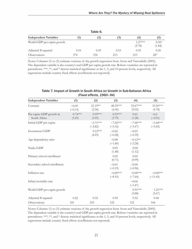
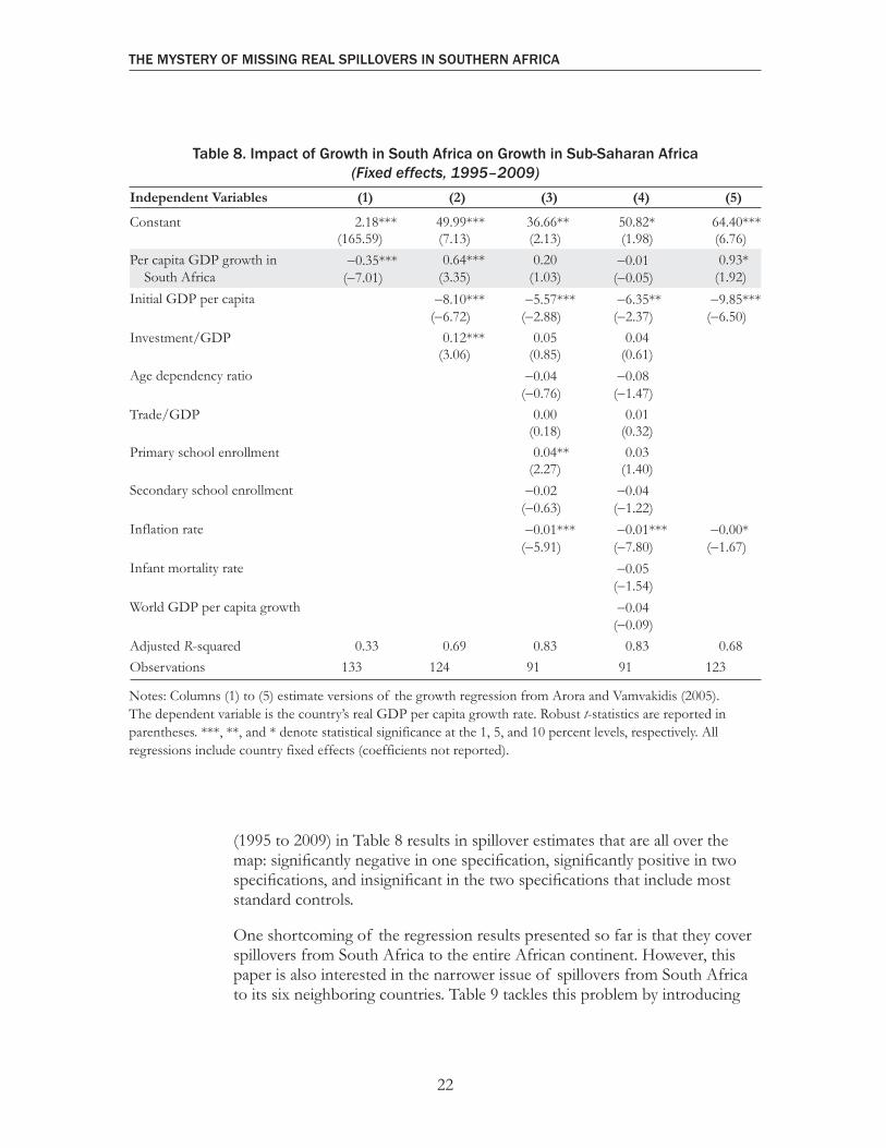
The results from the country-fi xed effects estimations ( Tables 6 to 8 ) are largely similar. Tables 6 and 7 fi nd large and signifi cant growth spillovers from South Africa to the rest of the continent over 1960 to 2009 and 1960 to 1994. Once again, the inclusion of global growth as a control reduces the estimates of South African growth spillovers, or even makes them statistically insignifi cant in Table 7 . Finally, focusing on the post-1994 period


21



Constant 0.05 21.19** 48.35*** 55.67*** 33.56***(0.15) (2.56) (4.36) (9.02) (4.78)

Per capita GDP growth in 0.74*** 0.59*** 0.93*** 0.61 0.2South Africa (3.43) (3.05) (3.79) (1.28) (0.91)

Initial GDP per capita 3.71*** 7.02*** 7.00*** 5.44***(2.82) (5.16) (5.47) (5.02)

Investment/GDP 0.12*** 0.02 0.03(4.23) (0.28) (0.39)

Age dependency ratio 0.08 0.12**(1.60) (2.28)

Trade/GDP 0.05 0.04(1.48) (1.12)


Secondary school enrollment 0.01 0.04(0.19) (0.96)

Inflation rate 0.00*** 0.00*** 0.00***(8.55) (7.64) (11.45)


World GDP per capita growth 0.91*** 1.21***(3.88) (5.67)


Notes: Columns (1) to (5) estimate versions of the growth regression from Arora and Vamvakidis (2005). The dependent variable is the country’s real GDP per capita growth rate. Robust t -statistics are reported in parentheses. ***, **, and * denote statistical significance at the 1, 5, and 10 percent levels, respectively. All regressions include country fixed effects (coefficients not reported).

Table 6.


World GDP per capita growth 1.27*** 0.56*(5.78) (1.84)




22



Constant 2.18*** 49.99*** 36.66** 50.82* 64.40***(165.59) (7.13) (2.13) (1.98) (6.76)

Per capita GDP growth in 0.35*** 0.64*** 0.20 0.01 0.93*South Africa (7.01) (3.35) (1.03) (0.05) (1.92)

Initial GDP per capita 8.10*** 5.57*** 6.35** 9.85***(6.72) (2.88) (2.37) (6.50)

Investment/GDP 0.12*** 0.05 0.04(3.06) (0.85) (0.61)


Trade/GDP 0.00 0.01(0.18) (0.32)

Primary school enrollment 0.04** 0.03(2.27) (1.40)


Inflation rate 0.01*** 0.01*** 0.00*(5.91) (7.80) (1.67)





(1995 to 2009) in Table 8 results in spillover estimates that are all over the map: signifi cantly negative in one specifi cation, signifi cantly positive in two specifi cations, and insignifi cant in the two specifi cations that include most standard controls.

One shortcoming of the regression results presented so far is that they cover spillovers from South Africa to the entire African continent. However, this paper is also interested in the narrower issue of spillovers from South Africa to its six neighboring countries. Table 9 tackles this problem by introducing


23

Table 9 . Impact of Growth in South Africa on Growth in Sub-Saharan Africa(Interactions with neighbor dummy, pooled panel, 1960–2009)


Constant 0.15 0.01 4.84 4.30***(0.36) (0.01) (1.20) (3.47)

BLMNSZ dummy 1.61*** 1.05 2.40 4.75(2.88) (0.39) (0.17) (1.44)

Per capita GDP growth in 0.68** 0.72*** 0.81*** 0.87***South Africa (2.54) (4.78) (4.46) (7.26)

Per capita GDP growth in 0.26 0.05 0.71 0.23South Africa × BLMNSZ dummy

(0.68) (0.12) 1.11 (0.86)

Initial GDP per capita 0.62*** 0.93*(2.75) (1.90)

Initial GDP per capita × 0.27 2.08**BLMNSZ dummy (0.67) (2.08)

Investment/GDP 0.21*** 0.21*** 0.18***(4.51) (3.54) (2.99)

Investment/GDP × BLMNSZ 0.09 0.23*** 0.16**dummy (1.10) (3.31) (2.39)

Age dependency ratio 0.041.46)

Age dependency ratio × 0.08BLMNSZ dummy (0.75)

Trade/GDP 0.03* 0.02**(1.87) (2.07)

Trade/GDP BLMNSZ 0.02 0.02dummy (1.06) (1.00)

Primary school enrollment 0.01(0.77)

Primary school enrollment × 0.03BLMNSZ dummy (0.49)


Secondary school enrollment × 0.1 0.01BLMNSZ dummy (1.61) (0.46)

Inflation rate 0.00*** 0.00***(7.84) (9.58)

Inflation rate BLMNSZ 0.01 0.03dummy (0.17) (0.55)

World GDP per capita growth 0.56*(1.79)

(continued )


24

a dummy variable that equals one when the country in question is one of the BLMNSZ countries, and zero otherwise. The BLMNSZ dummy is also interacted with all independent variables, in order to test for the possibility that regression coeffi cients for the BLMNSZ countries are signifi cantly different from those for other African countries. The results in Table 9 for the full sample (1960 to 2009) show clearly that there is no evidence of different spillover coeffi cients for South Africa’s six neighbors: all interaction terms with South Africa’s growth rate are not statistically signifi cant, while the coeffi cients on South Africa’s growth rate remain positive and signifi cant (as in Table 3 ). This fi nding matches the results in Arora and Vamvakidis (2005), who found that neither geographical proximity nor greater trade in goods explain spillovers from South Africa. In addition, we fi nd that the structural break in 1994 applies to South Africa’s neighbors, as it applies to everybody else on the continent. 6

Another possible criticism of the regression results reported thus far is that many of the covariates on the right-hand side of the regression equation are plausibly endogenous. In particular, South Africa’s growth rate might be endogenous to the growth rates of other African countries. To resolve the potential endogeneity problem, we employed two-stage least squares estimation using instrumental variables. As instruments, we used lagged values of South Africa’s growth rate, investment, and infl ation (all plausibly endogenous), as well as contemporaneous values of all other right-hand-side variables. Tables 10 to 12 report the results. In the full sample (1960 to 2009, Table 10 ), growth spillovers from South Africa are now typically insignifi cant.

Table 9 . Impact of Growth in South Africa on Growth in Sub-Saharan Africa(Interactions with neighbor dummy, pooled panel, 1960–2009)


World GDP per capita growth × 0.59BLMNSZ dummy (1.16)

Adjusted R-squared 0.06 0.30 0.39 0.38Observations 374 334 213 216

Notes: Columns (1) to (5) estimate versions of the growth regression from Arora and Vamvakidis (2005). The dependent variable is the country’s real GDP per capita growth rate. The Botswana, Lesotho, Mozambique, Namibia, Swaziland, and Zimbabwe (BLMNSZ) dummy is set to to equal one when the country is one of South Africa’s neighbors, and zero otherwise. The model in column (4) could not be estimated, due to a near-singular matrix. Robust t -statistics are reported in parentheses. ***, **, and * denote statistical significance at the 1, 5, and 10 percent levels, respectively.

6 These results are not reported here but are available upon request.

Table 9. (concluded)


25

Table 10 . Impact of Growth in South Africa on Growth in Sub-Saharan Africa(Two-stage least squares , 1960–2009)


Constant 0.73* 0.88 4.02 2.85**(1.92) (0.44) (0.89) (2.23)

Per capita GDP growth in 0.89** 0.60 0.19 0.41South Africa (2.11) (1.52) (0.44) (1.37)

Initial GDP per capita 0.39 0.75*(1.22) (1.78)

Investment/GDP 0.20*** 0.07 0.08(4.91) (0.75) (0.92)

Age dependency ratio 0.02(0.92)

Trade/GDP 0.03 0.03*(1.61) (1.83)



Inflation rate 0.00 0.00(1.48) (0.74)

Infant mortality rate

Landlocked dummy



Notes: Columns (1) to (5) estimate versions of the growth regression from Arora and Vamvakidis (2005). The model in column (4) could not be estimated, due to econometric problems caused by the large number of regressors and instruments. The dependent variable is the country’s real GDP per capita growth rate. Robust t -statistics are reported in parentheses. ***, **, and * denote statistical significance at the 1, 5, and 10 percent levels, respectively.

However, they are still positive and signifi cant in the pre-1994 sample ( Table 11 ). And they are statistically insignifi cant in the post-1994 sample ( Table 12 ) if we ignore columns (1) and (2), which report rather minimalist and stripped down versions of the regression equation. Overall, the story told by the earlier results (of growth spillovers disappearing circa 1994) survives this robustness check intact.


26



Constant 0.33 0.24 5.12 12.11***(1.03) (0.06) (1.00) (3.73)

Per capita GDP growth in 0.88** 1.01*** 0.98*** 0.83*South Africa (2.54) (4.91) (5.20) (1.71)

Initial GDP per capita 0.43 0.94 0.59(0.67) (1.36) (0.87)

Investment/GDP 0.15*** 0.08 0.01(3.63) (1.56) (0.19)

Age dependency ratio 0.02 0.04*(0.95) (1.82)

Trade/GDP 0.02* 0.02**(1.72) (2.01)


Secondary school enrollment 0.05 0.08*(1.53) (1.81)

Inflation rate 0.00 0.00*(0.89) (1.74)

Infant mortality rate 0.07***(3.09)


World GDP per capita growth 1.29***(5.93)



Our conclusion from reviewing and extending the literature is that there is no evidence that South Africa’s business cycle and its long-term growth rate affect those of its neighbors or the continent, at least not after 1994. While at fi rst surprising, this fi nding is in line with the broader literature on real spillovers. This literature is comprehensively summarized in Kalemli-Ozcan


27



Constant 2.30*** 1.91*** 4.56 6.86***(179.52) (2.81) (0.75) (2.73)

Per capita GDP growth in 0.11** 0.20*** 0.22 0.13South Africa (2.23) (3.25) (1.34) (1.15)

Initial GDP per capita 0.14 0.31(1.40) (0.60)

Investment/GDP 0.24*** 0.11 0.26***(4.11) (0.60) (4.44)

Age dependency ratio 0.01(0.58)

Trade/GDP 0.03(0.79)

Primary school enrollment 0.01**(2.07)

Secondary school enrollment 0.06**(2.04)

Inflation rate 0.01 0.00(0.97) (0.42)

Infant mortality rate 0.04**(2.57)

Landlocked dummy

World GDP per capita growth



and others (2013). They note that “many studies show that once we condition on common shocks (regional and global factors) and country fundamentals that do not change over time, the international output correlations are low. This refl ects the low degree of international spillovers of country-specifi c shocks in general.”

28

CHAPTERCHAPTER

Whodunit and Why?

There are a number of possible explanations for the econometric results summarized above. First, as already discussed, the economies of South Africa and the rest of the continent might have de-coupled around the mid-1990s, as international sanctions on South Africa ended and the country re-integrated with the world economy, while growth in the rest of the continent accelerated. Second, as suggested by the results in Kabundi and Loots (2007), the business cycles and trend growth rates of South Africa’s neighbors might be dominated by idiosyncratic shocks (Zimbabwe is perhaps the best example). Thus, the extent of trade, fi nancial, and institutional integration in Southern Africa might be more limited than conventional wisdom and summary statistics suggest. Third, the multiple spillover channels might operate in ways that offset each other, so that their net impact is relatively small. The remainder of this section discusses the key interconnections between South Africa and its neighbors, with an emphasis on these last two points (limited integration and multiple linkages pulling in opposite directions). The fl owchart in Figure 8 provides a summary of the arguments presented below. In the fl owchart, the plus, minus, and zero signs (+,−,0) denote, respectively, positive, negative, and zero correlation between GDP in South Africa and GDP in neighboring countries.

Trade Linkages

South Africa’s importance as a trade partner (see trade shares in Table 1 ) suggests a signifi cant positive correlation between South Africa’s business cycle and those of its neighbors. However, several caveats are in order. First, undifferentiated products traded on global markets (like most commodities) may be only marginally affected by slower demand in South Africa, as they can be easily diverted to other countries. Commodities constitute the bulk of what South Africa’s neighbors export, ranging from 43 percent in Mozambique to 93 percent in Botswana ( Table 1 ). Only four commodities (platinum, gold, diamonds, and tobacco) account for close to 60 percent of Zimbabwe’s

4

Whodunit and Why?

29

Figure 8 . A Flowchart Summarizing the Economic Linkages between South Africa and the Region

Linkagesbetween

South Africaand the region

Trade

Foreigndirect

investmentand financial

sector

Labormovements

andremi�ances

Monetaryand exchangerate policies

Fiscal

Large exports/imports with SA

Most exports are commodi�es

Net value added < gross exports

SA nonfinancial firms ac�ve in region

SA banks ac�ve in region

Migrant workers

SA monetary condi�ons

Procyclical SACU transfers

t + 2 adjustment delays spillovers

Remi�ances

Note: The plus, minus, and zero signs (+,−,0) denote, respectively, positive, negative, and zero correlation between GDP in South Africa and GDP in Botswana, Lesotho, Mozambique, Namibia, Swaziland, and Zimbabwe. SA = South Africa; SACU = Southern African Customs Union.

exports. Similarly, Swaziland’s exports to South Africa comprise mostly sugar, confectionery, and chemicals, all products that can easily be diverted to the rest of Africa or Europe.

Second, on a related note, land-locked countries (such as Botswana, Lesotho, Swaziland, and Zimbabwe) use South Africa’s ports in order to access international markets. In other words, while exports to South Africa from neighboring countries appear large, some of these fl ows of goods are probably not destined for fi nal consumption in South Africa. Rather, given South Africa’s status as an entrepôt center for the region, it is likely that a signifi cant fraction of these goods is processed and re-exported to the rest of the world. Hence, demand for these goods might be affected only slightly by a slowdown in South Africa’s economy. A good illustrative example would be South African imports of platinum ores from the region, which, after some processing and value addition, turn into South African exports of refi ned platinum or catalytic converters. Another example: textile and diamonds


30

account for 70 percent of Lesotho’s total exports and are mostly exported to the United States and Europe via South Africa.

Third, gross trade fl ows between South Africa and neighboring countries probably overstate the amount of net value addition that takes place in these countries. As mentioned above, many inputs used for the production of exports are imported from South Africa (electricity being a prime example). Thus, a decrease in South African demand for BLMNSZ exports may be partially offset by a decrease in their demand for imports from South Africa. The impact on the value added domestically will be smaller than the gross amount of exports would suggest.

Foreign Direct Investment and Financial Sector Linkages

South Africa is a key source of FDI for neighboring countries (see Table 1 ). In addition, South African nonfi nancial companies have a signifi cant presence in the region. A growth slowdown in South Africa might be propagated to the rest of the region via FDI outfl ows from these countries, especially if it weakens the balance sheets of South African fi rms. Or, it might force South African companies to explore more aggressively investment opportunities in neighboring countries, resulting in more South African FDI to the region (see The Economist , 2013).

South Africa–based banks dominate the banking sector in all neighboring countries ( Table 1 ). However, with a few exceptions, South Africa–based banks operate in neighboring countries via subsidiaries rather than branches. The choice of subsidiaries limits the scope for both inward and outward spillovers. 7 In addition, these subsidiaries have a strong preference for local banking, as largely domestic loans are typically funded with local deposits. Cross-border deposit-taking or loan-making is quite limited, with the exception of Swaziland and Lesotho, where cross-border deposits in South Africa are on the order of 10 to 20 percent of GDP ( Table 1 ). These features of the banking landscape in the Southern African region contain the scope for any regional fi nancial contagion due to a slowdown in South Africa.

We tested formally for fi nancial spillovers from South Africa to the region by looking at correlation coeffi cients between bank credit to the private sector in South Africa and bank credit to the private sector in BLMNS countries. We used quarterly data over 2003 to 2013, and we controlled for global shocks

7 Fiechter and others (2011) discuss the differences between branches and subsidiaries. An important caveat they make is that while those differences might appear stark on paper, in reality they tend to be more nuanced. For example, as illustrated during the Argentina crisis of 2001–2002, while subsidiaries might in theory be easier than branches for the parent to walk away from in a crisis, reputational risks and confidence effects might blur the distinction in practice.

Whodunit and Why?

31

by looking at bank credit to the private sector in each country relative to bank credit to the private sector in the United States. We also controlled for infl ation by defl ating each country’s numbers by the respective consumer price index (Zimbabwe was excluded due to hyperinfl ation). For one-year growth rates in private sector credit, the correlation coeffi cients between South Africa and BLMNS countries were generally low in absolute value. The only statistically signifi cant correlation coeffi cient (using a simple t -test test) was Swaziland’s at 0.32. We also found that if we exclude the period of the global fi nancial crisis, correlation coeffi cients tend to go down even further, thus confi rming that fi nancial spillovers are lower during normal times and higher in periods of fi nancial turmoil, a well-known result in the broader literature on spillovers. Finally, for annualized three-year growth rates (to account for spillover lags), the correlation coeffi cient for Swaziland was still signifi cantly positive, while those for Botswana and Mozambique were signifi cantly negative.

Institutional Linkages

As discussed in Chapter 1 , the BLNS countries effectively import their monetary and exchange rate policy from South Africa. If the growth slowdown in South Africa results in looser monetary policy, the associated depreciation of the rand would lower export prices and boost the competitiveness of BLNS countries on international markets in the short term.

Chapter 3 described how South African imports propagate a cyclical slowdown in South Africa to BLNS countries via the sharing of customs revenue under SACU. However, while growth in South Africa has been low in 2012 and 2013, imports have stayed robust, thus thwarting the operation of this propagation channel. In addition, a partially offsetting factor is the ex post adjustment made to year t SACU transfers in year t + 2 to correct for any discrepancy between transfers received in year t (based on import projections in year t − 1) and the level of transfers corresponding to the actual outturn. If year t turns out worse than was expected during year t − 1, this adjustment lag would delay the spillover effect of a slowdown in South Africa and reduce somewhat the procyclicality of SACU transfers. The role of SACU transfers as a transmission channel in Southern Africa is discussed in detail in Basdevant and others (2011) and Mongardini and others (2011).

32

Conclusion

South Africa has strong ties with its neighbors in the region. Thus, it is reasonable to expect that South Africa’s business cycle and trend growth rate will affect those of neighboring countries. While there are multiple linkages (trade, investment, fi nancial, and institutional) that are quantitatively important, formal econometric analysis in this paper and in the rest of the literature has not been able to detect a clear impact after 1994, once global shocks are controlled for. Moreover, we fi nd no evidence of real spillovers from South Africa to the rest of the continent over the same period. Plausible explanations include the limited extent of integration, the continent’s growth acceleration from the mid-1990s, the fact that South Africa’s growth impact may have become impossible to detect separately from global growth after South Africa reintegrated into the world economy with the end of sanctions, and the possibility that the multiple spillover channels pull in opposite directions. These stories are yet to be formally tested—a possible future extension of this paper. However, our gut feeling is that the decoupling in the mid-1990s and lagging integration are likely to turn out to be the main drivers behind our results.

The negative results of this paper are surprising and indeed counterintuitive. It is important not to exaggerate their signifi cance. The econometric estimates are based on historical data (whose quality is uneven). Given how fast the region and the continent are changing, the fi nding of no evidence of spillovers could change. The future might look quite different from the past.

33

References

Arora, V., and A. Vamvakidis, 2005, “The Implications of South African Economic Growth for the Rest of Africa,” IMF Working Paper WP/05/58 (Washington: International Monetary Fund).

———, 2010, “South Africa in the African Economy: Growth Spillovers,” Global Journal of Emerging Market Economies , Vol. 2, pp. 153–171.

Barro, R., and X. Sala-i-Martin, 1995, Economic Growth (New York: McGraw Hill).

Basdevant, O., D. Benicio, B. Mircheva, J. Mongardini, G. Verdier, S. Yang, and L.-F. Zanna, 2011, “The Design of Fiscal Adjustment Strategies in Botswana, Lesotho, Namibia, and Swaziland,” IMF Working Paper WP/11/266 (Washington: International Monetary Fund).

Canales-Kriljenko, J., F. Gwenhamo, and S. Thomas, 2013, “Inward and Outward Spillovers in the SACU Area,” IMF Working Paper WP/13/31 (Washington: International Monetary Fund).

The Economist , 2013, “The Grocers’ Great Trek: A Sluggish Home Market is Pushing South Africa’s Big Retail Chains Northward,” September 21.

Fiechter, J., I. Otker-Robe, A. Ilyina, M. Hsu, A. Santos, and J. Surti, 2011, “Subsidiaries or Branches: Does One Size Fit All?” IMF Staff Discussion Note SDN/11/04 (Washington: International Monetary Fund).

International Monetary Fund, 2012, “Nigeria and South Africa: Spillovers to the Rest of Sub-Saharan Africa,” in Regional Economic Outlook: Sub-Saharan Africa (Washington, October).

———, 2013, “Emerging Markets: Where Are They, and Where Are They Headed?” unpublished manuscript.

Kabundi, A., and E. Loots, 2007, “Co-movement between South Africa and the Southern African Development Community: An empirical analysis,” Economic Modelling , Vol. 24, pp. 737–748.

Kalemli-Ozcan, S., C. Erceg, B. Hunt, and M. Andrle, 2013, “Real and Financial International Spillovers,” unpublished (Washington: International Monetary Fund).

Kumhof, M., D. Laxton, D. Muir, and S. Mursula, 2010, “The Global Integrated Monetary and Fiscal Model (GIMF)—Theoretical Structure,” IMF Working Paper WP/10/34 (Washington: International Monetary Fund).

REFERENCES

34

Mongardini, J., D. Benicio, T. Fontaine, G. Pastor, and G. Verdier, 2011, “In the Wake of the Global Economic Crisis: Adjusting to Lower Revenue of the Southern African Customs Union in Botswana, Lesotho, Namibia, and Swaziland,” IMF African Department Discussion Paper 11/1 (Washington: International Monetary Fund).

United Nations Development Programme, 2010, “The Potential Contribution of the Zimbabwe Diaspora to Economic Recovery,” Comprehensive Economic Recovery in Zimbabwe Working Paper 11 (Harare: United Nations Development Programme).

The Mystery of Missing Real Spillovers in Southern Africa · 2014-06-04 · THE MYSTERY OF MISSING...

Documents

Transcript of The Mystery of Missing Real Spillovers in Southern Africa · 2014-06-04 · THE MYSTERY OF MISSING...