The Multiplicative Weyl Functional Calculus - CORE · THE MULTIPLICATIVE WEYL FUNCTIONAL CALCULUS...
18
JOURNAL OF FUNCTIONAL ANALYSIS 9,423-440 (1972) The Multiplicative Weyl Functional Calculus ROBERT F. V. ANDERSON Department of Mathematics, University of British Columbia, Vancouver 8, Canada Communicated by the Editors Received April 26, 1971 The Weyl calculus discussed in the author’s previous papers starts with a fixed set of n noncommuting self-adjoint operators and associates an operator to a real function of n variables. The calculus is not multiplicative with respect to point-wise multiplication of functions. However, if the rr self-adjoint operators generate a unitary Lie group representation, a “skew product” of functions can be defined which yields multiplicativity. This skew product depends only on the Lie group, not on the particular representation. In the case of the Heisenberg group, this skew product makes it possible to write the Schriidinger equation as an integro-differential equation on the phase plane. Strong convergence of the dynamical group, as Plan&s constant goes to zero, to the classical Hamiltonian flow is proved under various conditions on the Hamiltonian. 1. INTRODUCTION The linear correspondence between functions in the Schwartz class Y(P) and operators on Hilbert space 3 induced by an n-tuple of self-adjoint operators A = (A, ,..., A,) according to the formula x exp(--i(SA + -*a + 5A)) 45 e-0 dt, (1.1) is discussed in [I] and [2]. All notations are carried over from those papers. A functional calculus usually has a multiplicative property of the form f(A) g(A) = (fg)(A), where (fg)(x) = f(x) g(x). This is impos- sible for the Weyl calculus defined by formula (l.l), because, in general, f(A) and g(A) d o not commute except in the trivial case when A is an n-tuple of commuting operators. In this paper, a productf*g will be defined such that (f*g)(A) = 423 0 1972 by Academic Press, Inc.
Transcript of The Multiplicative Weyl Functional Calculus - CORE · THE MULTIPLICATIVE WEYL FUNCTIONAL CALCULUS...

JOURNAL OF FUNCTIONAL ANALYSIS 9,423-440 (1972)
The Multiplicative Weyl Functional Calculus
ROBERT F. V. ANDERSON
Department of Mathematics, University of British Columbia, Vancouver 8, Canada
Communicated by the Editors
Received April 26, 1971
The Weyl calculus discussed in the author’s previous papers starts with a fixed set of n noncommuting self-adjoint operators and associates an operator to a real function of n variables. The calculus is not multiplicative with respect to point-wise multiplication of functions. However, if the rr self-adjoint operators generate a unitary Lie group representation, a “skew product” of functions can be defined which yields multiplicativity. This skew product depends only on the Lie group, not on the particular representation. In the case of the Heisenberg group, this skew product makes it possible to write the Schriidinger equation as an integro-differential equation on the phase plane. Strong convergence of the dynamical group, as Plan&s constant goes to zero, to the classical Hamiltonian flow is proved under various conditions on the Hamiltonian.
1. INTRODUCTION
The linear correspondence between functions in the Schwartz class Y(P) and operators on Hilbert space 3 induced by an n-tuple of self-adjoint operators A = (A, ,..., A,) according to the formula
x exp(--i(SA + -*a + 5A)) 45 e-0 dt, (1.1)
is discussed in [I] and [2]. All notations are carried over from those papers.
A functional calculus usually has a multiplicative property of the form f(A) g(A) = (fg)(A), where (fg)(x) = f(x) g(x). This is impos- sible for the Weyl calculus defined by formula (l.l), because, in general, f(A) and g(A) d o not commute except in the trivial case when A is an n-tuple of commuting operators.
In this paper, a productf*g will be defined such that (f*g)(A) =
423 0 1972 by Academic Press, Inc.
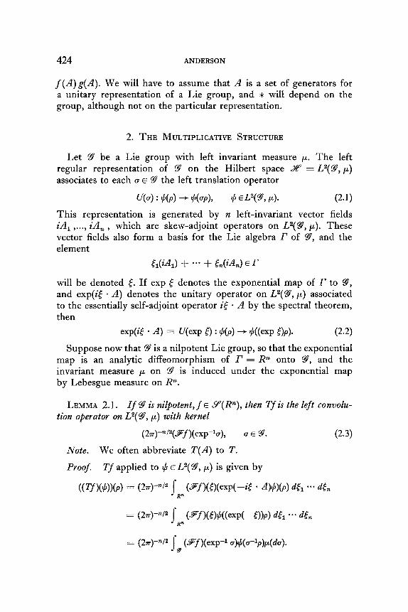
424 ANDERSON
f(A)g(A). We will have to assume that A is a set of generators for a unitary representation of a Lie group, and * will depend on the group, although not on the particular representation.
2. THE MULTIPLICATIVE STRUCTURE
Let 93 be a Lie group with left invariant measure p. The left regular representation of ‘3’ on the Hilbert space Z = L2(‘3, p) associates to each o E 93 the left translation operator
7-44 : %%J> - v+f), 4 E wg, 4. (2.1)
This representation is generated by n left-invariant vector fields iA 1 ,..., i& , which are skew-adjoint operators on L2(9, p). These vector fields also form a basis for the Lie algebra r of ~9, and the element
5&A,) + --* + &&&) E r
will be denoted [. If exp 5 denotes the exponential map of r to 9, and exp(i[ + A) d enotes the unitary operator on L2(9, p) associated to the essentially self-adjoint operator it * A by the spectral theorem, then
exp(i5 - 4 = U(exp 0 : 4(f) -+ #((exp 0~). (2.2)
Suppose now that 3 is a nilpotent Lie group, so that the exponential map is an analytic diffeomorphism of I’ = R” onto 9, and the invariant measure ,u on 93 is induced under the exponential map by Lebesgue measure on R”.
LEMMA 2.1. If 99 is nilpotent, f E Y(R”), then Tf is the left convolu- tion operator on L2(9, p) with kernel
(2~)-+(9-~)(exp-lo), (TEC??. (2.3)
Note. We often abbreviate T(A) to T.
Proof. Tf applied to # E L2(9?, p) is given by
V~)W))(P) = PFz s FW(O(exp(-~~ - 4#)(~) d& -*a 45 R”
= PF J^ (~ff(EM((exp(-c3l~) 45 a** dL R”
= (2v)+j2 I, (Ff)(exp-i u)#(u-lp)p(du).

THE MULTIPLICATIVE WEYL FUNCTIONAL CALCULUS 425
LEMMA 2.2. If 99 is nilpotent, and f, g E Y(R”), there is a unique h E Y(R”) such that
n = vf)m.
Explicitly, h = F-IK, where
K(5) = (2+@ j (@If)(exp-‘(exp(-4 exp tW%9(77) 4. (2.4) R"
Also, the map (f, g) -+ h is a continuous map
Y(R") x sqP(Ry + Y(P).
Proof.
wfv..N~~(P>
= (W~/2 j, (4"lf>(exP 4 ~d~)(~-lf W4
= (2?r)+j2 j, (Ff)(exp-l u)
x [(2r)-“j2 j, (Fg)(exp” 6)#(~-~8-lp)p(dS)] I.
Replace g by a-la to obtain
(2~)-” j,,, (~~>(exp-l(slu))(~g)(exp-l QNu-~P>P(W~W
= (2~r-“/~ 1, [(2~)-~/~ j, (gf)(exp-1(8-1u))(*g)(exp-1 +(&)I
x ~(eJlPP~-
The convolution within the brackets equals K(5) as defined in (2.4), where 5 = expel u and 7 = exp-l 6. Note that
exp(-7) = 6-l.
Since 3 is nilpotent, exp-l(exp(--7)) exp .$) is a polynomial in 7 and E, by the Campbell-Baker-Hausdorff Theorem. Therefore K( 8) is C”, and by elementary estimates, K(f) E Y(R”). Therefore h = F-lK E Y(R”). The lemma then follows from Lemma 2.1. Uniqueness of h is obvious, since different convolution kernels give

426 ANDERSON
different operators. 9 is a homeomorphism of Y(P), so the last statement also follows from (2.4) by easy estimates.
DEFINITION. h is called the skew product off and g, and denoted
f*g-
THEOREM 2.3. Lemma 2.2 holds for the Weyl calculus of the generators of any strongly continuous unitary representation of 3.
Proof. Let the representation be g ---t V(g), with generators iA = (iA, ,..., iA,), so that
V : exp(E) -+ exp(it * A).
G?fKcg) = Pw2 j,,,,. PVM)(~gh) exp(-if - 4 exp(--iv * 4 dt 4.
With 77 fixed, the map
5 - exp-Yexp(-7) exp 8 = 45 7)
is induced by left translation by exp(--r)) in ‘3, and therefore preserves Lebesgue measure in Ii”. Also
-4!,71) = exp-l((exp(-7) exp f)-‘) = exP(ew(-t) exp 77);
so
exp( --ih(f, 7) * A) = exp(-;E * A) exp($ . A).
Therefore,
(Tf x%9 = PW j,.,,, CV)(W d>(~‘)(d exp(-% 7) . A) exp(+ . A) 8 dq
= cw” j,,,,. PTf>GG, rl)P%M exp(--if . 4 d5 4
= (27+n/2 j Rn
[(2+n/2 j Rn
(--Ff>(#, rl))(~g)(d dq] exp(-Gt . 4 d5
and the content of the brackets equals formula (2.4).
Remark. Let 3 be any Lie group, and f, g E 9(R”). By the proof of Lemma 1.1, Tf can be represented, when iA generates the left regular representation, as left convolution on L2(~, II) with a measure

THE MULTIPLICATIVE WEYL FUNCTIONAL CALCULUS 427
whose total variation is at most (2?~)+/~ I/ 9fllLl . The convolution of the measures representing Tf, Tg is also a measure which, as a convolution operator, represents (Tf )( Tg). However, when 99 is not nilpotent, it is not obvious that this measure is Th for any h E Y(R”), or, when h E Y(RRn) does exist, that it is unique.
A “local” skew product can always be defined. For any 9, there is always a ball B(0, Y) C Rn = r centered at 0 E r with radius Y > 0, such that exp restricted to B(0, Y) is a diffeomorphism onto a neigh- bourhood N of the identity in 9. Let M be a smaller neighbourhood such that M2 C N. Then if Ff, Sg are supported in exp-l M, the measures Tf, Tg are given by formula (1.2) and are in Cow(M). Their convolution is in C,,“O(M2) C Cam(N). It follows that there is a unique h E Y(Rn) such that Th is supported in B(0, r) and Th = (Tf)(Tg). N ow exp-l M contains a ball B(0, s) C r. By the Paley-Wiener theorem, this means that if f, g extend to entire analytic function on Cn with bounds of the form cesiimr~, then there is a unique h E Y(R”) extending to an entire function bounded by erlimzl and such that
The same generalization applies to Theorem 2.3. Note that if 3 is a semisimple group, the exponential map is
periodic on certain one-parameter subgroups and singular only at a discrete subgroup of such a group. This makes it easy to construct counter examples to uniqueness of h E Y(Rn).
EXAMPLES. On L2(R1), let translation be denoted by S(t) : p)(x) --f ~(x + t), and let M(p(x)) denote the unitary multiplier exp(ip(x)), where P(X) is a polynomial in x of degree <m. The unitary operators on L2(R1) of the form U(p, t) = M(p(x)) S(t) form a group g(m) since
and
w, 4 w, 0 = Wd4 + P(X + wqs + q
(2.5) U(p, Q-1 = S(-t)M(--p(x)) = M(-p(x - t))S(-t).
If P(X) = a,xm + *** + a,, then (a0 ,..., anz , t) are coordinates with respect to which the group operation is analytic, so 3(m) is a Lie
group. The representation of 9’(m) by itself is strongly continuous on L2(R1), and is generated by the (m + 2)-tuple iA, where
A = i 1, x ,..., x”, 4 &).
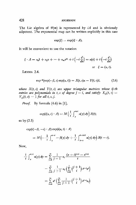
428 ANDERSON
The Lie algebra of 9(m) is represented by iA and is obviously nilpotent. The exponential map can be written explicitly in this case
exp($ = exp(if * A).
It will be convenient to use the notation
( - A = 0~~1 + ollx + ... + or,xna + t (-ii) = a(x) + t (-i-g)
or .$ = (a, t).
LEMMA 2.4.
exp-l(exp(-+, s) exp(a, t)) = X(t, s)a - Y(t, s)/3,
where X(t, s) and Y(t, s) are upper triangular matrices entries are polynomials in t, s of degree j - i, and satisfy Yii(t, s) = 1 for all t, s, j.
Proof. By formula (4.6) in [l],
P-6)
whose ij-th Xii(t, s) =
exp(i(a, t) * A) = M (+ /:‘t a(Y) dy) s(t);
so by (2.5)
exp(i(+, -S) * A) exp(i(cr, t) * A)
Now,
1
s
s+t (x + t)i+l - $+I
-L O(y) dy = f L "j
j&o i + 1 t

THE MULTIPLICATIVE WEYL FUNCTIONAL CALCULUS 429
and
aj (i (j 1 ‘)( 5 ) t+s)k-i)) k=i
Let a(t) be the (m + 1) x (m + 1) matrix with entries aij(t) defined for 0 < i, j < m by
1 1
Q&(t) = ; + l ( 1 i + 1 ti-i
i i<j
i>j.
Similarly define a(t, s) with
qt, s) = 0 i>j.
Then
exp(i@, -s) . A) exp(i(a, t) * A) = M(9Y(t, -s)ct - OZ(--s)/?)S(t - s).
Therefore
exp-l(exp(i@ - s) * A)) exp(i(ol, t) . A)
= qt - s)-qt, -+)a - qt - s)-a?( -s)/3.
Note that for all t, s, G!(t) and B(t, s) are upper triangular, with ~2~~ = 3Yjj = 1 for all j, and that ~2?~~(t) and gij(t, s) are polynomials in s, t homogeneous of degree j - i. In particular,
where J(t) is diagonal and Iii(t) = ti. Therefore,
W(t) = J-l(t)@-l(l)](t),

430 ANDERSON
so that (a-l(t)), = (P1(l)),itj-i. It follows that if we define
X(t, s) = a-yt - s)LB(t, -s),
Y(t, s) = a-yt - s)aT(-s).
X and Y have the required properties.
THEOREM 2.5. For 9(m), use coordinates (X0 ,..., X, , u) or (x, u) on Rn dual to (01~ ,..., ol,, t) E r. Let fu(x, w) denote f(x, u + w). Let S&::f denote the partial Fourier transform off (x, w) with respect to w.
(f * g>(x, 4 = & j,, (~m+,fu>(W, 4x> W=m+~gW(--s> --Ox, 4 ds 4 (2.7)
where Z(s, t) = Q!*(t) SV*(t + s, -s). In particular,
0 i <j,
&(t, s) = l i=j,
polynomial in s, t i>j, homogeneous of degree i - j.
Note. GP denotes adjoint GZ.
Proof. Formulas (2.4) and (2.6) yield
Wf * gm, 0
= (24++ j (=?f>(x(t, ~>a - y(t, @, t - s)(Fg)(& s) d/3 ds Rn
= (24-V j,, [(2+w
We will now work with the content of the brackets in the last

THE MULTIPLICATIVE WEYL FUNCTIONAL CALCULUS 431
expression, keeping t, s fixed and suppressing the dependence of X, Y on t, S. The bracket equals
(24-(7+1)/2 j,,-, [(2X)-(n--1)lP j,.-, ei(XQ-YB)‘Z(~~+lf)(X, t - s) dx]
x (~A@> 4 4
= (2++1)/2 jRnel ei(X*r).o(Fm+lf)(x, t - s)
x [(24+)/z j p-l
e-i’y*z).B(Pg)(j3, s) d,!?] dx
= (27+l”-1)/2 j eicx*x)‘~(~,+,f)(~, t - s)(Fm+lg)( Y*x, s) dx. p-1
This becomes, on replacing x by X*x, (a volume preserving change of variable),
(2~)+-1)/2 jRm_, ei~.~(Pm+lf)(X-l*x, t - s)(Fm+lg)((XwlY)*x, S) dx
= e..... m((~m+lf>(x-l*X, t - s)(~*t+lg)((x-ly)*x, 4).
Therefore
(f * &9(x, 4
1 -- - s 27r R2
e-i”u(Fm+lj)(X-l*(t, s)x, t - s)(St,+,g)(X-lY)*(t, s)x, s) ds dt.
Replacing t by t + s yields
& j (~m+Jiu>(X-l*(t + s, 4x, t)(*m+lgw)(X-ly)*(t + s, SIX, s) ds dt. R=
It remains to show that X-l*(t + S, s) = .Z(t, s), and
(X-lY)*(t + s, s) = q-s, -t).
By the defining formulas for X, Y,
X-l*(t, s) = a*(t - s)sF*(t, -s),
(X-lY)*(t, s) = m(-sp-l*(t, -s).
432
Therefore,
ANDERSON
x-l*(t + s, s) = a*(t)sFl*(t $
(X-lY)*(t + s, s) = a*(-s)el*(t
It suffices to show c%(t + s, -s) = B’( g(t + s, -s), is the matrix associated with
s, -s), t s, -4.
- -s - t, t). However, the polynomial in X, t) is associated with l/(t + s) JzLi 01( y) dy. Therefore, 9#( --s - t,
l/(--s - t) C;: c( y) dy w tc o h’ h b viously equals the foregoing.
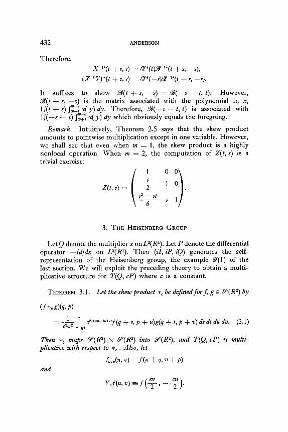
Remark. Intuitively, Theorem 2.5 says that the skew product amounts to pointwise multiplication except in one variable. However, we shall see that even when m = 1, the skew product is a highly nonlocal operation. When m = 2, the computation of Z(t, S) is a trivial exercise:
3. THE HEISENBERG GROUP
Let Q denote the multiplier x onLa(R1). Let P denote the differential operator -id/dx on L2(R1). Th en (iI, iP, iQ) generates the self- representation of the Heisenberg group, the example 9?(l) of the last section. We will exploit the preceding theory to obtain a multi- plicative structure for T(Q, cP) where c is a constant.
THEOREM 3.1. Let the skew product *C be de$ned for f, g E csP( R2) by
(f *c gk PI
1 =- C%T2 I
e2i(sv-tu)/cf(q + s, p + u)g(q + t, p + v) ds dt du dv. (3.1) R4
Then *e maps 9’(R2) x Y(R2) into 9(R2), and T(Q, cP) is multi- plicative with respect to *C . Also, let
fP,&, v) = f(u + 4, v + PI and
V&U, v) = f (7 ) - 7).
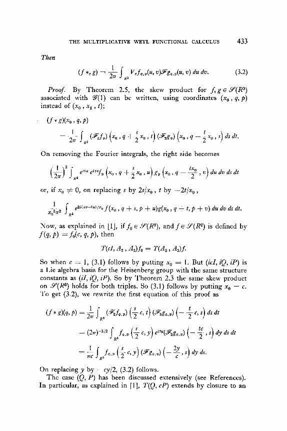
THE MULTIPLICATIVE WEYL FUNCTIONAL CALCULUS 433
Then
(f *cd = & j,, ~cfo.&, 4~cdu, 4 du da (3.2)
Proof. By Theorem 2.5, the skew product for f, g E Y(P) associated with 99( 1) can be written, using coordinates (x0 , 4, p) instead of (x0 , x1 , t);
(f * d@o Y 43 P)
= & j,, (%f,) bo > q + ; xo 9 t) b%g,> (~0 , q - ; xo , s) ds dt.
On removing the Fourier integrals, the right side becomes
1 2 i-1 s 257 eitU eisvfz, x0, q + i x0, u x0, q - F, v du dv ds dt R4
or, if x0 # 0, on replacing s by 25/x, , t by -2t/x, ,
1 -I X0279
e2i(sv-tu)/zof(xo , q + S,P + u)g(x,, , q + t, p + V) du dv ds dt. R4
Now, as explained in [I], if f. E Y(R3), and f E Y(R2) is defined by
f (4, P) = fO(G 4, P), then
WA A2 9 A3)fo = v, , 4)f'
So when c = 1, (3.1) follows by putting x0 = 1. But (icl, iQ, iP) is a Lie algebra basis for the Heisenberg group with the same structure constants as (i1, iQ, iP). So by Theorem 2.3 the same skew product on SP(R3) holds for both triples. So (3.1) follows by putting x,, = c. To get (3.2), we rewrite the first equation of this proof as
(f*g)(q,~) = & jR2 (%f,,.) & t) P5gu.J (- + s)dsdt
= (2+3’2 jR,fQ,D ($ c,.y)@(%g,,,) (- 4, s)& dsdt
On replacing y by -cy/2, (3.2) follows. The case (Q, P) has b een discussed extensively (see References).
In particular, as explained in [l], T(Q, cP) extends by closure to an

434 ANDERSON
isometry of L2(R2) onto the Hilbert-Schmidt (HS) operators, except for a scalar factor:
(3.3)
Let iB generate a unitary group U(t) of operators. Then the group of inner automorphisms of the Hilbert algebra HS, C(t) = U(t) CU(-t) is the solution of the passive form of the Schrodinger equation
$ C(t) = i(BC(t) - C(t)B) E i[B, C(t)]. (3.4)
It is therefore natural to look at the equation
ds . 1 dt = 4f*g -g *f) = $L~l (3.5)
induced on L2(R2) by inverting the map (i/c) T(Q, cP). However, the generator B is not usually HS; so we should make a suitable extension of the skew product, using (3.2), and the simple fact that
g*f=J*&
DEFINITION. Let f E Y’(R2), g E Y(R2). Let f [ g] denote the action off on g. Then
(f * gk, P> = & (~Cf&,W&.,l, (3.6)
[f,gl =f *g -3*c (3.7)
LEMMA 3.2. Let frz Y'(R2),g, k E Y(R2). Then f*g E P(R2) and is polynomially bounded, and
(f*d*~=f*k*4, (f*d[~l =fk *4 ([f, glP1 = f Kg, 41.
Proof. For the first statement, it suffices that each seminorm on Y applied to (V$9gp,P)-p,-P be polynomially bounded, a fact which is clear by inspection. The remaining statements are simple exercises in multiple integration.
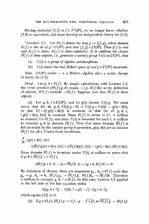
THE MULTIPLICATIVE WEYL FUNCTIONAL CALCULUS 435
Having extended (3.5) to f E 9’(R2), we no longer know whether (3.4) is equivalent, and must develop an independent theory for (3.5).
THEOREM 3.3. Let H(f) denote the map g + i[f, g], whose domain 6?(f) is the set of g E L2(R2) such that [f, g] E L2(R2). Then if f is real and 8(f) is dense, H(f) is skew-symmetric. If in addition the closure H( f ) is skew-adjoint, i.e., generates a unitary group U(t) on L2(R2), then
(a) U(t) is a group of algebra automorphisms
(b) U(t) leaves the real Hilbert space of real g E L2(R2) invariant.
Note. L2(R2) under * is a Hilbert algebra after a scalar change of norm, by (3.3).
Proof. Let g, k E a( f ). By simple calculations with Lemma 3.2, the inner product (H(f) g, k) equals -(g, H(f)k); so by definition of adjoint, H*(f) extends - H( f ). Suppose now that H(f) is skew adjoint.
(a) Let g, k, 1 ELM, and let g(t) denote U(t) g. We must prove that for all g, k, U(t)( g * k) = U(t) g * U(t)k = g(t) * k(t), or that U(-t)( g(t) * k(t)) is constant, or that for all g, k, 1, ( g(t) * k(t), l(t)) is constant. Since 6(f) is dense in L2, it suffices to consider 1 E &( f ), and since U(t) is bounded for each t, it suffices to consider g, k in domain H( f ). Note that since domain H(f) is left invariant by the unitary group it generates, g(t), k(t) are in domain g(f) for all t. Under these conditions,
yg- (g(t) * 4th l(t))
= @w&w) * 4th l(t)> +MwPxt)~ l(t)) + (g(t) * k(t), mf)l)(w
Since domain R(f) is invariant under U(t), it suffices to prove that ifg,kEB(f), 1 ~g(f),
(i-f(f)g * 4 1) + (g * fJ((f)k 1) + (g * k, R(f)l) = 0.
By definition of closure, there are sequences g, , k, E a(f) such that
gm -g, 42 - 4 H(f) g, -a( H(f)& + R(f)k. Therefore it suffices to consider g, k, 1 E 8(f). In this case, Lemma 3.2 applied to the left side of the last equation yields
fb!, k * VI +fl+, i *gll +.tI--irg * k Ill which equals f [0] or 0.
@I IfgE&(f),H(f)g = i(f*g -f?);soH(f)g = H(f)8

436 ANDERSON
Therefore, Re g E 8( f ), and Re(H(f)g) = H(f)(Reg). By closure,
Reowk) = fmw d for g E domain a(f).
Therefore,
-g Peg(O) = Jw(Re g(t)) if g E domain E(f).
Therefore, Reg(t) = U(t)(Reg(O)) = U(t)g = g(t), if g is real and in domain R(f). S’ mce the set of such g is dense in the real L2(R2) space, the theorem follows.
We have now lifted Schrodinger’s equation to the phase plane, getting a dynamical equation
(3.8)
for each value of c, and a unitary group UC(t) if EC(f) is skew-adjoint. If the Hamiltonian f is a C1 function h(q,p), we can compare UC(t) with the group Us(t) generated by the classical Hamiltonian vector field ahlap a/aq - ah/aq alap. In view of Theorem 3.3(b), we can assume g is real-valued.
LEMMA 3.4. Let h(q,p) b e a C2 function whose second partial derivatives are polynomially bounded. Then if g E Y(R”), the pointwise limit
holds uniformly on compact domains in R2.
Proof. By formula (3.6), and the fundamental theorem of calculus,
+ Hc@k
=&~,,(h,.,(+ -7) -hm++~))Stg,,,(u,v)dudv
i =-s s 112 277 R2 (ZI, -u) . (grad h)Q,P(cOv, -A) dBPg,&u, v) du dv
-l/Z
1 - ss
112 --
23-r g2 (grad h),,,(cOv, -cOti) * (S(gag),,,)(u, v) d0 du dv,
-l/2
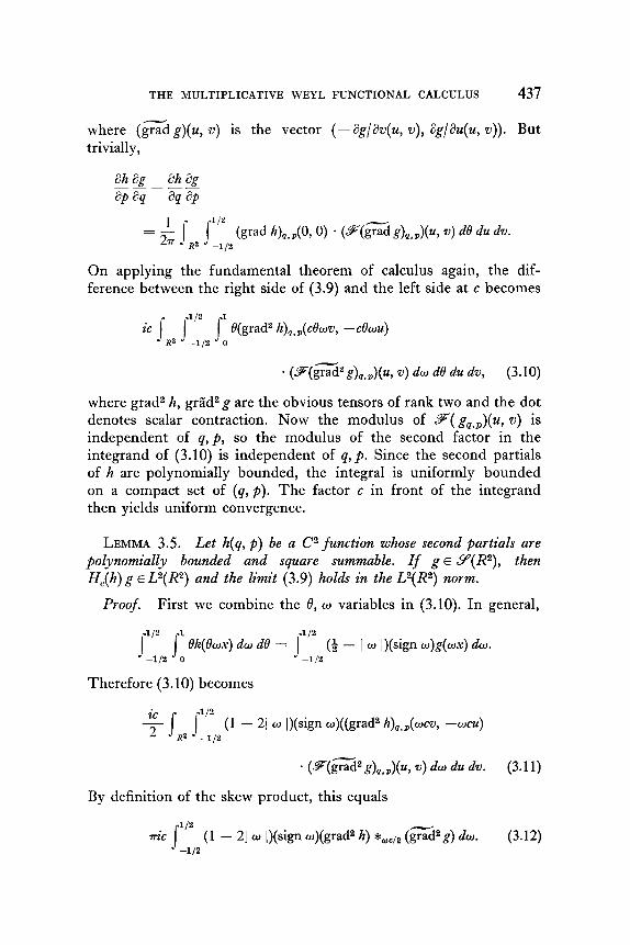
THE MULTIPLICATIVE WEYL FUNCTIONAL CALCULUS 437
where (gx g)(u, U) is the vector (- 3g/ik(u, v), ag/ih(u, v)). But trivially,
ah ag ah ag ----- 8~ a4 a4 3~
1 =- s s
“’ 277 R2
(grad h),,,(O, 0) . (p(gs g)p,J(u, w) d8 du dv. -l/2
On applying the fundamental theorem of calculus again, the dif- ference between the right side of (3.9) and the left side at c becomes
ic s,, cl;, J: B(grad2 h),,,(c&v, -43~~)
. (cF(gzz g),,,)(u, v) dw dt’ du dv, (3.10)
where grad2 h, grPd2 g are the obvious tensors of rank two and the dot denotes scalar contraction. Now the modulus of s( g,,,)(u, V) is independent of q,p, so the modulus of the second factor in the integrand of (3.10) is independent of q,p. Since the second partials of h are polynomially bounded, the integral is uniformly bounded on a compact set of (q,p). The factor c in front of the integrand then yields uniform convergence.
LEMMA 3.5. Let h(q, p) be a C2 function whose second partials are polynomially bounded and square summable. If g E Y(R2), then
f&(h) g E L2(R2) and the limit (3.9) holds in the L2(R2) norm.
Proof. First we combine the 8, w variables in (3.10). In general,
f” 1’ Bh(Bwx) dw d0 = j”’ (4 - 1 w /)(sign w)g(wx) dw. -l/2 0 -l/2
Therefore (3.10) becomes
iC
-s s “’
2 (1 - 21 w I)(sign w)((grad2 h)q,D(Wcv, -UCU)
R2 -l/2
. (*(grad2 g),,,)(u, v) dw du dv. (3.11)
By definition of the skew product, this equals
s 112
iTiC (1 - 21 w I)(sign w)(grad2 h) *Wc,2 (a2 g) dw. (3.12) -l/2

438 ANDERSON
By (3.3), jig *,k \I2 < l/1/% I/g 11s Ij k /I2 ; so we get an L2 norm estimate for (3.12):
z-cII grad2 h II2 /j gz2g [I2 1”’ -l/2
(1 - 21 w I) -$==== &A = l/c * constar& 7Tf.d
which goes to zero as c --+ 0.
LEMMA 3.6. Suppose that h(q, p) is a polynomial or has the form V(q), where V(q) has a polynomially bounded continuous second deriva- tive. If g E Y(R2), then H,(h) g E L2(R2) and (3.9) holds in the L2(R2) norm.
Proof. If h is a polynomial homogeneous of degree s, inspection of (3.6) shows that H,(h) is a partial differential operator of degree s carrying a factor cs. Therefore, H,(h)g is a polynomial in c with coefficients in Y(R2) and, therefore, converges in L2 as c -+ 0. By Lemma 3.4, the limit is the required one. If h(q, p) = V(q), then formula (3.11) reduces to
(1 - 21 w I)(sign CO) -I,2
- ei(gu+pv) (9 (-$)) (u, w) dw du dw
ic f
112 =-
2 (1 - 21 w /)(sign w)r(q,p, w) dw, -112
where
r(q, P, w) = --& j,, elpv $ (Q + wcv) (% (3)) (4,~) dw.
Since r(q, p, w) is written as a partial Fourier integral of
4% w, w> = $F (4 + ,co> (% ($) (4, +,
therefore with w fixed,
II Y(S P, 412 = It S(P, v, 4ii2 . But Pz( a2g/ a$“) E Y(R2) and d2V/dq2 is polynomially bounded. Therefore, II Sk, v, w)IIz is bounded when w and c are bounded. The
THE MULTIPLICATIVE WEYL FUNCTIONAL CALCULUS 439
factor c in front of the original integrals then gives the L2 convergence to zero.
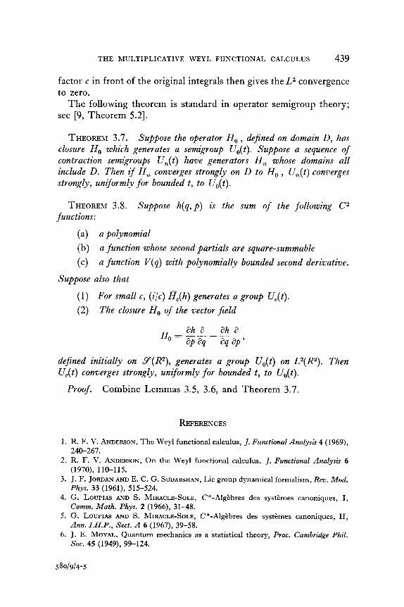
The following theorem is standard in operator semigroup theory; see [9, Theorem 5.21.
THEOREM 3.7. Suppose the operator HO , dejined on domain D, has closure RO which generates a semigroup U,,(t). Suppose a sequence of contraction semigroups Un(t) have generators H, whose domains all include D. Then if H, converges strongly on D to H,, , U%(t) converges strongly, uniformly for bounded t, to Uo(t).
THEOREM 3.8. Suppose h(q,p) is the sum of the following C2 functions :
(a) a polynomial
(b) a function whose second partials aye square-summable
(c) a function V(q) with p ly o nomially bounded second derivative.
Suppose also that
(1) For small c, (i/c) H,(h) generates a group UC(t).
(2) The closure g,, of the vector jield
H =ah?!-!!!ha 0 8P % &I 3P ’
dejined initially on SP(R2), generates a group U&t) on L2(R2). Then UC(t) converges strongly, uniformly for bounded t, to U,,(t).
Proof. Combine Lemmas 3.5, 3.6, and Theorem 3.7.
REFERENCES
1. R. F. V. ANDERSON, The Weyl functional calculus, J. Functional Analysis 4 (1969), 240-267.
2. R. F. V. ANDERSON, On the Weyl functional calculus, J. Functional Analysis 6 (1970), 110-115.
3. J. F. JORDAN AND E. C. G. SUDARSHAN, Lie group dynamical formalism, Rev. Mod. Phys. 33 (1961), 515-524.
4. G. LOUPIAS AM) S. MIRACLE-SOLE, C*-Algebres des systemes canoniques, I, Comm. Math. Phys. 2 (1966), 31-48.
5. G. LOUPIAS AND S. MIRACLE-SOLE, C*-Algebres des systemes canoniques, II, Ann. I.H.P., Sect. A 6 (1967), 39-58.
6. J. E. MOYAL, Quantum mechanics as a statistical theory, Proc. Cambridge Phil. Sot. 45 (1949), 99-124.
440 ANDERSON
7. J. C. T. POOL, Mathematical aspects of the Weyl correspondence, J. Math. Phys. 7 (1966), 66-76.
8. I. E. SEGAL, Transforms for operators and symplectic automorphisms over a locally compact abelian group, Math. Stand. 13 (1963), 31-43.
9. H. TROTTER, Approximation of semigroups of operators, Pacific J. Math. 8 (1958), 887-919.
10. E. WIGNER, On the quantum correction for thermodynamic equilibrium, Phys. Rev. 40 (1932), 749-759.