The Multilevel Latent Covariate Model: A New, More …The Multilevel Latent Covariate Model: A New,...

The Multilevel Latent Covariate Model: A New, More ReliableApproach to Group-Level Effects in Contextual Studies

Oliver LudtkeMax Planck Institute for Human Development

Herbert W. MarshOxford University

Alexander RobitzschInstitute for Educational Progress

Ulrich TrautweinMax Planck Institute for Human Development

Tihomir AsparouhovMuthen & Muthen

Bengt MuthenUniversity of California, Los Angeles

In multilevel modeling (MLM), group-level (L2) characteristics are often measured by aggregat-ing individual-level (L1) characteristics within each group so as to assess contextual effects (e.g.,group-average effects of socioeconomic status, achievement, climate). Most previous applicationshave used a multilevel manifest covariate (MMC) approach, in which the observed (manifest)group mean is assumed to be perfectly reliable. This article demonstrates mathematically and withsimulation results that this MMC approach can result in substantially biased estimates of contex-tual effects and can substantially underestimate the associated standard errors, depending on thenumber of L1 individuals per group, the number of groups, the intraclass correlation, the samplingratio (the percentage of cases within each group sampled), and the nature of the data. To addressthis pervasive problem, the authors introduce a new multilevel latent covariate (MLC) approachthat corrects for unreliability at L2 and results in unbiased estimates of L2 constructs underappropriate conditions. However, under some circumstances when the sampling ratio approaches100%, the MMC approach provides more accurate estimates. Based on 3 simulations and 2real-data applications, the authors evaluate the MMC and MLC approaches and suggest whenresearchers should most appropriately use one, the other, or a combination of both approaches.

Keywords: multilevel modeling, contextual analysis, latent variables, structural equationmodeling, Mplus

Supplemental materials: http://dx.doi.org/10.1037/a0012869.supp

In the last 2 decades multilevel modeling (MLM) hasbecame one of the central research methods for applied

researchers in the social sciences. A major advantage ofMLMs over single-level regression analysis lies in the pos-sibility of exploring relationships among variables locatedat different levels simultaneously (Goldstein, 2003; Rau-denbush & Bryk, 2002; Snijders & Bosker, 1999). In thetypical application of MLM, outcome variables are relatedto several predictor variables at the individual level (L1;e.g., students, employees) and at the group level (L2; e.g.,schools, work groups, neighborhoods).

Different types of group-level variables can be distin-guished. The first type can be measured directly (e.g., classsize, school budget, neighborhood population). These vari-ables that cannot be broken down to the individual level areoften referred to as “global” or “integral” variables(Blakely & Woodward, 2000). The second type is generatedby aggregating variables from a lower level. For example,ratings of school climate by individual students may beaggregated at the school level, and the resulting mean can be

Oliver Ludtke and Ulrich Trautwein, Center for EducationalResearch, Max Planck Institute for Human Development, Berlin,Germany; Herbert W. Marsh, Department of Education, OxfordUniversity, Oxford, United Kingdom; Alexander Robitzsch, Insti-tute for Educational Progress, Humboldt University, Berlin;Tihomir Asparouhov, Muthen & Muthen, Los Angeles, California;Bengt Muthen, Graduate School of Education & Information Stud-ies, University of California, Los Angeles.

We thank Marcel Croon, Harvey Goldstein, and David Kennyfor comments on earlier versions of this article and Susannah Gossfor editorial assistance.

Correspondence concerning this article should be addressed toOliver Ludtke, Max Planck Institute for Human Development,Center for Educational Research, Lentzeallee 94, 14195 Berlin,Germany. E-mail: [email protected]

Psychological Methods2008, Vol. 13, No. 3, 203–229

Copyright 2008 by the American Psychological Association1082-989X/08/$12.00 DOI: 10.1037/a0012869

203

used as an indicator of the school’s collective climate.Variables that are obtained through the aggregation ofscores at the lower level are known as contextual or ana-lytical variables. For instance, Anderman (2002), using alarge data set with students nested within schools, examinedthe relations between school belonging and psychologicaloutcomes (e.g., depression, optimism). School belongingwas included in the multilevel regression model as both anindividual (L1) characteristic and a school (L2) character-istic. School-level belonging was based on the within-school aggregation of individual perceptions of school be-longing. In a similar vein, Ryan, Gheen, and Midgley(1998) related student reports of avoidance of help-seekingto student and classroom goals (for other applications, seeHarker & Tymms, 2004; Kenny & La Voie, 1985; Ludtke,Koller, Marsh, & Trautwein, 2005; Miller & Murdock,2007; Papaioannou, Marsh, & Theodorakis, 2004).

Croon and van Veldhoven (2007) have emphasized theapplicability of these issues to many subdisciplines of psy-chology, including educational, organizational, cross-cul-tural, personality, and social psychology. Iverson (1991)provided a brief summary of the extensive application ofcontextual analyses in sociology, dating as far back asDurkheim’s study of suicide and including topics as diverseas the racial composition of neighborhoods, village use ofcontraceptives, local crime statistics, political behavior inelection districts, families in the study of socioeconomicstatus (SES) and schooling, volunteer organizations,churches, workplaces, and social networks. In fact, theissues are central to any area of research in which individ-uals interact with other individuals in a group setting, lead-ing Iverson to conclude: “This range of areas illustrates howbroadly contextual analysis has been used in the study ofhuman behavior” (p. 11).

In the MLM literature, models that include the samevariable at both the individual level and the aggregatedgroup level are called contextual analysis models (Boyd &Iverson, 1979; Firebaugh, 1978; Raudenbush & Bryk, 2002)or sometimes compositional models (e.g., Harker &Tymms, 2004). The central question in contextual analysisis whether the aggregated group characteristic has an effecton the outcome variable after controlling for interindividualdifferences at the individual level. The effects of the L1characteristic may or may not be of central importance,depending on the nature of the study and the L1 construct(e.g., Papaioannou et al., 2004).

One problematic aspect of the contextual analysis model isthat the observed group average obtained by aggregating indi-vidual observations may not be a very reliable measure of theunobserved group average if only a small number of L1individuals is sampled from each L2 group (O’Brien, 1990;Raudenbush, Rowan, & Kang, 1991). For instance, in educa-tional research, where only a small proportion of studentsmight be sampled from each participating school, the observed

group average is only an approximation of the unobserved“true” group mean—a latent variable. When MLMs are used toestimate the contextual analysis model, it is typically assumedthat the observed L2 variables based on aggregated L1 vari-ables are measured without error. However, when only a smallnumber of L1 units are sampled from each L2 group, the L2aggregate measure may be unreliable and result in a biasedestimate of the contextual effect.

In the present study we introduce a latent variable ap-proach, implemented in the latent variable modeling soft-ware Mplus (Asparouhov & Muthen, 2006; B. O. Muthen,2002; L. K. Muthen & Muthen, 2007; but see also B. O.Muthen, 1989; Schmidt, 1969), which takes the unreliabilityof the group mean into account when estimating the con-textual effect. Because the group average is treated as alatent variable, we call this approach the multilevel latentcovariate (MLC) model. In contrast, we label the “tradi-tional” approach, which relies solely on the (manifest) ob-served group mean, the multilevel manifest covariate(MMC) model. The term manifest indicates that this ap-proach treats the observed group means as manifest anddoes not infer from them to an unobserved latent constructthat controls for L2 unreliability.

Our article is organized as follows. We start by distin-guishing between reflective and formative L2 constructs.We then give a brief description of how the MMC is usuallyspecified in MLMs, outlining the factors that affect thereliability of the group mean and deriving mathematicallythe bias that results from using the MMC approach toestimate the contextual effect. After introducing the MLCmodel as it is implemented in Mplus, we summarize theresults of simulation studies comparing the statistical prop-erties of the latent and manifest approaches. In addition, wepresent analyses comparing the Croon and van Veldhoven(2007) two-step approach to our (one-step) MLC approach.We then present two empirical examples using both thelatent and the manifest approaches. Finally, on the basis ofall of these results, we offer suggestions for the appliedresearcher and propose directions for further research.

Reflective and Formative L2 Constructs

We argue that the appropriateness of the MLC approachdepends in part on the nature of the construct under study. Forthe present purposes, we propose a distinction between forma-tive and reflective aggregations of L1 constructs (for moregeneral discussion of formative and reflective measurement,see Bollen & Lennox, 1991; Edwards & Bagozzi, 2000; Kline,2005; also see Howell, Breivik, & Wilcox, 2007). Althoughour choice of terms is based on a factor analytic rationale, arelated distinction is made in the organizational psychologyliterature (e.g., Bliese, 2000; Bliese, Chan, & Ployhart, 2007;also see Kozlowski & Klein, 2000) between compilation (orconfigural) models and composition models.

204 LUDTKE ET AL.

Formative (compilation or configural) aggregations of L1constructs are considered to be an index of L1 measureswithin each L2 group (i.e., arrows in the underlying struc-tural equation model go from the L1 indicators to the L2construct; e.g., Kline, 2005). Formative constructs have thefollowing characteristics: The focus of L1 measures is on anL1 construct, L1 individuals within the same L2 group arelikely to have different L1 true scores, and scores fordifferent individuals within the same L2 group are notinterchangeable. There is no expectation that the individuallevel and aggregated variables reflect the same construct;thus, corresponding L1 and L2 measures are not assumed tobe isomorphic. For formative aggregated L2 constructs,variation among individuals can be thought of as a substan-tively important group characteristic (i.e., groups are rela-tively heterogeneous or homogeneous in relation to a spe-cific L1 characteristic). Particularly when the sampling ratio(the percentage of L1 individuals considered within each L2group) approaches 100%, it is inappropriate to use variationwithin each L2 group (intraclass correlation [ICC]) to esti-mate L2 unreliability due to sampling error. Whereas thefocus of our research has been on the mean as an aggregatesummary used to construct a group (L2) construct, Kozlow-ski and Klein (2000) emphasize that various indexes of L1constructs within a group could be used as the L2 aggre-gated (formative) measure (e.g., minimum, maximum, vari-ation, profile similarity, system dynamics, etc.). For exam-ple, let us assume that a researcher wants to evaluate thegender composition of students in each of a large number ofdifferent classes and has information for all students withineach class. An appropriate L2 aggregate variable (e.g.,percentage of girls) can be measured with essentially nomeasurement or sampling error at either L1 or L2. Studentswithin each class are clearly not interchangeable in relationto gender, and even if a particular class—by chance ordesign—happens to have a disproportionate number of boysor girls, this feature of the class reflects a true characteristicof that class rather than unreliability due to sampling error.Hence, as emphasized by Kozlowski and Klein (2000), itmight be appropriate to consider measures of within-groupheterogeneity (diversity) as a potentially useful L2 aggre-gated (formative) construct. Examples of formative L2 ag-gregated constructs might include L2 aggregations of L1characteristics such as race, age, gender, achievement lev-els, SES, or other background/demographic characteristicsof individuals within a group. Making a similar point, Bliese(2000) noted that for pure compilation-based aggregatemeasures (similar to our formative L2 variables), there is noassumption of within-group agreement and that measures ofreliability based on within-group agreement tend to be ir-relevant in establishing the construct validity of the L2measures.

Reflective (or compositional) aggregations of L1 con-structs have the following characteristics: The purpose of

L1 measures is to provide reflective indicators of an L2construct, all L1 indicators (typically different individualswithin the same group) within each L2 group are designedto measure the same L2 construct, and scores associatedwith different individuals within the same L2 group areinterchangeable. The L2 construct is assumed to “cause” theL1 indicators (i.e., arrows in the underlying structural modelgo from the latent L2 construct to the L1 indicators). Thus,reflective aggregations are analogous to the typical latentvariable approach based on classical measurement theoryand the domain sampling model (Kline, 2005; Nunnally &Bernstein, 1994), in which multiple indicators (in this case,multiple persons within each group rather than the multipleitems for each construct) are used to infer a latent constructthat is corrected for unreliability (based on the number ofindicators and the extent of agreement among the multipleindicators) that would otherwise result in biased estimates.Hence, the concept of reflective measurement is consistentwith the notion of a generic group-level construct that ismeasured by individual responses (Cronbach, 1976; Croon& van Veldhoven, 2007). Under these conditions, it isreasonable to use variation within each L2 group (ICC) toestimate L2 sampling error that includes error due to finitesampling and error due to a selection of indicators (i.e., aspecific constellation of individuals used to measure agroup-level construct). Within-group variation representslack of agreement among individuals within the same groupin relation to an L2 construct rather than a substantivelyimportant characteristic of the group. Examples of reflectiveL2 constructs might include individual ratings of classroom,group, or team climate; individual ratings of the effective-ness of a teacher, coach, or group leader; individual markerratings of the quality of written compositions, perfor-mances, artwork, grant proposals, or journal article submis-sions. Within the organizational psychology literature, theterm referent shift measures (Chan, 1998; Chen, Bliese, &Mathieu, 2005) is used to denote the case in which thereferent for a measure shifts from that of the individual (e.g.,individual self-efficacy) to that of the group (the efficacy ofthe group as a whole). Particularly when the referent of themeasures is the group as a whole, the resulting aggregatedmeasures might be considered a reflective (or composi-tional) construct.

The distinction between formative and reflective variablesis particularly important in climate research (for furtherdiscussion, see Papaioannou et al., 2004). For example, if allindividual students within each of a large number of differ-ent classes are asked to rate the competitive orientation oftheir class as a whole, the aggregated L2 construct might bemost appropriately represented as an L2 reflective construct.The observed measure is designed to reflect the L2 constructdirectly and is not intended to reflect a characteristic of theindividual student. However, if each individual student isasked to rate his or her own competitive orientation, the

205CONTEXTUAL ANALYSIS

aggregated L2 construct might be more appropriately con-sidered as a formative L2 construct. The observed L1 mea-sure is designed to reflect an L1 construct rather than to bea direct measure of an L2 construct, even if the L2 aggre-gation of the L1 measures is used to infer an L2 construct.We would expect agreement among different ratings bystudents within the same class (ICC) to be substantiallyhigher for the L2 reflective construct than for the corre-sponding L2 formative construct. Whereas lack of agree-ment among students within the same class on the L2reflective variable can be used to infer L2 unreliability, lackof agreement on the L2 formative construct reflects within-class heterogeneity in relation to an L1 construct.

Bliese (2000) argued that pure compositional models (likeour L2 reflective aggregation measures) require completeisomorphism in which every group member provides ex-actly the same score so that there is no variation withingroups on the relevant L1 construct. Noting that cases ofpure isomorphism between L1 and L2 constructs are ex-tremely rare (except, perhaps, in highly artificial situations),he described a “‘fuzzy’” composition construct involvingboth compositional and compilation processes. Similarly,we contend that L2 constructs based on an aggregation ofL1 constructs vary along a continuum in which pure reflec-tive and pure formative constructs represent the endpoints.Although we focus on the endpoints of the continuum, wenote that most L2 aggregated constructs fall somewherebetween the reflective and formative endpoints of this con-tinuum. We also note that we chose the terms formativeversus reflective because these terms have better establishedmeanings in the psychometric literature in relation to theunderlying structural equation model used to define them. Incontrast, there is less consistency in the use of the compi-lation (or configural) versus composition models in theorganizational psychology literature (Bliese, 2000; Kozlow-ski & Klein, 2000). Indeed, aggregated variables resultingfrom a formative aggregation process such as SES or stockmarket indexes are commonly referred to as compositemeasures, which is the exact opposite of the implicit mean-ing of compositional models in the organizational psychol-ogy literature. Nevertheless, our use of a formative–reflec-tive continuum of L2 aggregated constructs is essentiallythe same as the pure compositional to pure compilationalcontinuum used by Bliese (2000) in his discussion of fuzzycompositional L2 aggregated variables.

Contextual Analysis

The Contextual Analysis Model in MultilevelModeling

In this section, we provide a short description of thecontextual analysis model in the traditional multilevelframework. We assume that we have a two-level structure

with persons nested within groups and an individual-levelvariable X (e.g., socioeconomic status) predicting the de-pendent variable Y (e.g., reading achievement). Applyingthe MLM notation as it is used by Raudenbush and Bryk(2002), we have the following relation at the first level:

Level 1: Yij��0j��1j(Xij�X� •j)�rij, (1)

where the variable Yij is the outcome for person i in groupj predicted by the intercept �0j of group j and the regressionslope �1j in group j. The predictor variable Xij is centered atthe respective group mean X� •j. This group-mean centering ofthe individual-level predictor yields an intercept equal to anexpected value of Yij for an individual whose value on Xij isequal to his or her group’s mean. At Level 2, the L1intercepts �0j and slopes �1j are dependent variables:

Level 2: �0j � �00 � �01X� •j � u0j

�1j � �10, (2)

where �00 and �10 are the L1 intercepts and �01 is the sloperelating X� •j to the intercepts from the L1 equation. As can beseen, only the L1 intercepts have an L2 residual u0j. MLMsthat allow only the intercepts to deviate from their predictedvalue are also called random-intercept models (e.g., Rau-denbush & Bryk, 2002). In these models, group effects areallowed to modify only the mean level of the outcome forthe group; the distribution of effects among persons withingroups (e.g., slopes �1j) is left unchanged. Now inserting theL2 equations into the L1 equation we have

Yij � �00 � �10�Xij � X� •j� � �01X� •j � u0j � rij. (3)

This notation is referred to as the linear mixed-effect nota-tion (McCulloch & Searle, 2001) and is used, for example,by the mixed module in SPSS and similar procedures inother statistical packages. Equation 3 reveals that the maindifference between a single-level regression analysis and anMLM lies in the more complex error structure of the mul-tilevel specification. Furthermore, it is now easy to see that�10 is the within-group regression coefficient describing therelationship between Y and X within groups and that �01 isthe between-groups regression coefficient that indicates therelationship between group means Y� •j and X� •j (Cronbach,1976). A contextual effect is present if �01 is higher than�10, meaning that the relationship at the aggregated level isstronger than the relationship at the individual level.

Grand-mean centering. Another approach to test for acontextual effect (which is mathematically equivalent undercertain conditions; see Raudenbush & Bryk, 2002) is to usea different centering option for the individual-level predic-tor. Instead of using group-mean centering of the predictorvariables—where the group mean of the L1 predictor issubtracted from each case—researchers often center the

206 LUDTKE ET AL.

predictor at its grand mean. In grand-mean centering, thegrand mean of the L1 predictor is subtracted from each L1case. Substituting the group-mean X� •j in Equation 3 by thegrand-mean X� •• gives the following model:

Yij � �00 � �10�Xij � X� ••� � �01X� •j � u0j � rij. (4)

In contrast to the group-mean centered model, where thepredictor variables are orthogonal, the predictors �Xij

� X� ••� and X� •j in this grand-mean centered model are notindependent. Thus, �10 is the specific effect of the groupmean after controlling for interindividual differences on X.Note that, in the grand-mean centered model, the individualdeviations from the grand mean, �Xij � X� ••�, also includethe person’s group deviation from the grand mean. Conse-quently, a contextual effect is present if �01 is statisticallysignificantly different from zero. However, it can be shownthat, in the case of the random-intercept model, the group-mean model and the grand-mean centered model are math-ematically equivalent (see Kreft, de Leeuw, & Aiken,1995). For the fixed effects, the following relation holds forthe L2 between-groups regression coefficient: �01

grandmean

� �01groupmean � �10

groupmean. The within-group regressioncoefficient at Level 1 will be the same in both models:�10

grandmean � �10groupmean. Hence, the results for the fixed

part of the grand-mean centered model can be obtained fromthe group-mean centered model by a simple subtraction.1

Because our analysis is limited to random-intercept models,centering of predictor variables will not be a critical issue inour article. In the remainder of the article, our investigationof the analysis of group effects in MLM focuses on thegroup-mean centered case.

The reliability of the group mean for reflective aggrega-tions of L1 constructs. One problematic aspect of thecontextual analysis model, as described earlier, is that theobserved group average X� •j might be a highly unreliablemeasure of the unobserved true group average because onlya small number of L1 individuals are sampled from each L2group (O’Brien, 1990). For reflective aggregations of L1constructs, the reliability of the aggregated L2 construct asa measure of the “true” group mean depends on at least twoaspects: the proportion of variance that is located betweengroups—measured by the ICC—and the number of individ-uals in the group (Bliese, 2000; Snijders & Bosker, 1999).

In the multilevel literature, the ICC is used to determinethe proportion of the total variance that is based upondifferences between groups (Raudenbush & Bryk, 2002).The ICC is based on a one-way analysis of variance(ANOVA) with random effects, where the outcome on L1 isthe dependent variable and the grouping variable is theindependent variable. The ICC is defined as follows:

ICC ��2

�2 � 2, (5)

where �2 is the variance between groups and 2 is thevariance within groups. Thus, the ICC indicates the propor-tion of total variance that can be attributed to between-groups differences.

For reflective aggregations of L1 constructs, the reliabil-ity of the aggregated data X� •j is estimated by applying theSpearman–Brown formula to the ICC, with n being thenumber of persons per group (Bliese, 2000; Snijders &Bosker, 1999):

L2 Reliability �X� •j� �n � ICC

1 � �n � 1� � ICC. (6)

As can be seen, the reliability of X� •j (Equation 6) for reflec-tive aggregations of L1 constructs depends on two factors: theproportion of variance that is located between groups (ICC)and the group size (n). In most cases, the mean group size canbe entered for n if not all groups are of the same size (seeSearle, Casella, & McCulloch, 1992, on how to deal withpronounced differences in group size). For example, assumingthat students in 50 classes rate their mathematics instruction,the ICC indicates the reliability of an individual student’srating—sometimes referred to as the single-rater reliability(Jayasinghe, Marsh, & Bond, 2003; Marsh & Ball, 1981). Thereliability of the class-mean rating can be estimated by theSpearman–Brown formula, with n being the number of stu-dents per class. As is apparent from Equation 6, the reliabilityof the class-mean rating increases with the number of students(n). In other words, the more students in a class provide ratings,the more reliably the class-mean rating will reflect the truevalue of the construct being measured. It is worth noting thatEquation 6, which determines the reliability of the observedgroup mean, says nothing about the reliability of the L1 mea-sure. In general, measurement error at Level 1 results in lowerreliability of the group means (Raudenbush et al., 1991). How-ever, Equation 6 does not differentiate between L1 variancethat is due to measurement error and L1 variance that is due totrue differences between L1 individuals. For reflective aggre-gations of L1 constructs, the assessment of L2 unreliability dueto sampling error is—as noted above—analogous in manyways to traditional approaches to reliability based on multiple,interchangeable indicators of each latent construct (i.e., withmultiple persons as interchangeable indicators of each latentgroup mean).

Bias of the between-groups regression coefficient forreflective aggregations of L1 constructs. Let us now as-sume that a contextual model holds in the population andthat the within-group and between-groups relationships aredescribed by the within-group regression coefficient �within

1 A little more algebra is needed for the conversion of thevariance components (see Kreft et al., 1995). Note that the modelsare no longer equivalent in either the fixed part or the random partwhen random slopes or nonlinear components are allowed.


and the between-groups regression coefficient �between (seeSnijders & Bosker, 1999, p. 29). We want to estimate thesecoefficients by sampling a finite sample of L2 groups fromthe population. In the next stage, a finite sample of L1individuals is obtained for each sampled L2 group. Bearingin mind the previous formula for the reliability of the groupmean, results from the literature on regression analysissuggest that the regression coefficient for the L2 averagewill be biased. Applying standard results from theory onlinear models (Seber, 1977), the expected bias of the within-and between-groups regression coefficients in a contextualanalysis model can be determined depending on the reli-ability of the group mean. Because it is assumed that theindividual-level variable is measured without error for re-flective aggregations of L1 constructs, the within-groupcoefficient is an unbiased estimator. In contrast, it can beshown that the between-groups coefficient �01 is a biasedestimator of the between-groups coefficient �between (for thederivation, see the Appendix):

E��01 � �between� � ��within � �between� �1

n

��1 � ICC�

ICC � �1 � ICC�/n. (7)

The relationship between the expected bias and the ICC aswell as the group size is depicted in Figure 1 for �within ��between values of .2, .5, and .8. In all three panels, the biasbecome smaller with larger group sizes n. In other words,when the group mean is more reliable due to a higher n,�between can be more precisely approximated by the mani-fest group mean predictor. The bias also decreases as theICC increases. As shown in Equation 6, the reliability of thegroup mean is a direct function of the group size n and theICC. Indeed, for sufficiently large cluster sizes, the differ-

ence between the manifest and latent approaches will betrivially small, even for reflective factors. The bias in thebetween-groups coefficient has direct consequences for theestimation of the “true” contextual effect for reflective ag-gregations of L1 constructs. In the group-mean centeredmodel, the contextual effect is calculated as the difference,�01 – �10, between the between-groups regression coeffi-cient �01 and the within-group coefficient �10. Assumingperfect measurement of the group mean, this would corre-spond to a “true” difference of �between � �within. It followsthat the bias of the estimated contextual effect can beexpressed by:

E��01 � �10� � ��between � �within�

� ��within � �between� �1

n�

�1 � ICC�

ICC � �1 � ICC�/n. (8)

This relationship indicates that the contextual effect in thepopulation will be underestimated by the contextual analy-sis model if �within �between. However, if �within ��between, the contextual effect will be positively biased.2

Thus, a low ICC together with small samples of L1 indi-viduals from each L2 group will affect the bias of contextualeffect considerably.

In the approach to contextual analysis for reflective ag-gregations of L1 constructs outlined above, the group-level

2 This constellation is present in research on the so-called frog-pond effect (Davis, 1966). The most prominent example is the big-fish–little-pond effect: the observation that individual student achieve-ment has a substantially positive effect on academic self-concept,whereas the effect of school- or class-average achievement is consis-tently negative (Marsh & Hau, 2003). As is apparent from Equation8, the big-fish–little-pond effect is probably underestimated in abso-lute terms when the manifest covariate approach is applied.

Figure 1. Relationship between the expected bias of the between-groups regression coefficient, thenumber of Level 1 units within each Level 2 unit (n), and the intraclass correlation coefficient (ICC)of the predictor for three different values of �within � �between.

208 LUDTKE ET AL.

predictor was formed by aggregating all of the observedmeasurements in each group (MMC approach). In the nextsection, we introduce an alternative approach to contextualanalysis that infers the latent unobserved group mean fromthe observed data and that takes into account the unreliabil-ity of the group mean (L2 sampling error) when estimatingthe contextual effect (MLC approach). Historically, nearlyall contextual effect studies have used an MMC approach,due in part to technical limitations in most statistical pack-ages that made a latent covariate approach difficult to for-mulate. With the enhanced flexibility of MLM programssuch as Mplus, however, it is now possible to introduce andevaluate an MLC approach (but see Croon & van Veld-hoven, 2007, for an alternative implementation). Hence, thepurpose of this article is to demonstrate the MLC approach,to evaluate statistical properties with simulated data, toillustrate its application with two actual (real-data) exam-ples, and to critically evaluate its appropriateness from atheoretical and philosophical perspective.

A Multilevel Latent Covariate (MLC) Model

The concept of latent variables was originally introducedin the social and behavioral sciences to represent entitiesthat may be regarded as existing but cannot be measureddirectly (e.g., Lord & Novick, 1968). For instance, in psy-chometric research, intelligence is considered a latent vari-able that cannot be directly observed but can only be in-ferred from the participants’ observed behavior in tests. Inthese traditional psychometric applications, the values of alatent variable represent participants’ scores on a trait orability. Recently, several methodologists have proposed thatthe conceptualization of latent variables be broadened toinclude other circumstances in which unobserved individualvalues might profitably be included in the model (B. O.Muthen, 2002; Raykov, 2007; Skrondal & Rabe-Hesketh,2004). In this latent variable framework, latent class mem-bership and missing data are just two examples of latentvariables.

The flexibility of this modeling framework is expressed inthe definition provided by Skrondal and Rabe-Hesketh (2004,p. 1): “We simply define a latent variable as a random variablewhose realizations are hidden from us.” As a consequence ofthis generality, the latent variable framework is able to inte-grate MLM and structural equation modeling (SEM; seeRaykov, 2007, for an application to longitudinal analysis) andis currently implemented, for example, in the Mplus (L. K.Muthen & Muthen, 2007) and GLLAMM (Skrondal & Rabe-Hesketh, 2004) software. In the present study, we used theMLC approach to consider the group effect as an unobservedlatent variable that has to be inferred from the observed data.More specifically, the unobserved group mean is regarded as alatent variable that is measured with a certain amount ofprecision by the group mean of the observed data (Asparouhov

& Muthen, 2006). As is typical within SEM, the estimate of thegroup-level coefficient is then corrected for the unreliablemeasurement of the latent group mean by the observed groupmean. In the present study, our MLC approach was imple-mented using a maximum likelihood procedure in Mplus,which provides estimates that are consistent and asymptoti-cally efficient within a very flexible approach to estimatinglatent variable models.3

The basis for the latent covariate approach is that eachvariable is decomposed into unobserved components, whichare considered latent variables (Asparouhov & Muthen,2006; B. O. Muthen, 1989; Schmidt, 1969; Snijders &Bosker, 1999; see also Rabe-Hesketh, Skrondal, & Pickles,2004). The dependent variable Y and the independent vari-able X can be decomposed as follows:

Xij � �x � Uxj � Rxij

Yij � �y � Uyj � Ryij, (9)

where �x is the total mean of X, Uxj are group-specificdeviations, and Rxij are individual deviations. The samedecomposition holds for Y. Note that Xij and Yij are observedvariables, whereas Uxj, Uyj, Rxij, and Ryij are unobserved. Weare interested in estimating the relationship between theseunobserved variables at the individual and the group level:

Ryij � �withinRxij � εij

Uyj � �betweenUxj � j. (10)

The two equations can be combined into one by substitutingEquation 10 into Equation 9. The dependent variable Y isthen predicted by the individual and group-specific devia-tions:

Yij � �y � Uyj � Ryij � �y � �betweenUxj

� �withinRxij � j � εij. (11)

It is now easy to see that Equation 11 is approximated by thegroup-mean centered model expressed by Equation 3,

3 The version of Mplus (Version 4.2) used in the present investi-gation is based on an accelerated EM algorithm for analysis ofmaximum likelihood estimation of a two-level structural equationmodel with missing data (Asparouhov & Muthen, 2003). This modelincorporates random coefficients and integrates the modeling frame-works of hierarchical linear models and two-level structural equationmodels. It provides robust estimates of the asymptotic covariance ofthe maximum likelihood estimates and the chi-square test. Note thatthe models considered here can be fitted with the approach describedby Lee and Poon (1998) that handles only random-intercept modelsbut that Mplus takes a more general approach with random slopes (seealso supplemental materials available online for a more detaileddescription).


which is based on observed variables. The latent unobservedgroup deviation Uxj corresponds to the observed groupmeans X� •j and the individual deviation Rxij to �Xij � X� j�.

It is worth noting that the latent covariate approach tocontextual analysis can also be implemented in traditionalmultilevel programs such as HLM or MLwiN by using astepwise procedure (Goldstein, 1987; Hox, 2002). In thefirst step, a within- and between-groups covariance matrix isestimated using a multivariate MLM. Hox (2002) demon-strated how a multivariate model can be estimated usingMLM software designed to estimate univariate models (fora recent application of a multivariate MLM, see Bauer,Preacher, & Gil, 2006). In the second step, the within- andbetween-groups coefficients are estimated based on thesecovariance matrices.4 Of course, the multivariate approachis much more limited than the implementation of the latentcovariate approach in Mplus in that it can only be appliedeasily to random-intercept models.

Recently, Croon and van Veldhoven (2007) proposed atwo-stage latent variable approach. The unobservedgroup mean for each L2 unit is calculated using weightsobtained from applying basic ANOVA formulas. Theseadjusted group means form the basis for an ordinary leastsquares (OLS) regression analysis at the group level.Croon and van Veldhoven showed analytically and bymeans of simulation studies that an OLS regression anal-ysis based on the observed group means results in biasedestimates, whereas the results based on the adjustedgroup means are unbiased. However, in contrast to ourfull information maximum likelihood (FIML) MLC ap-proach, their two-stage procedure is only a limited infor-mation approach. The model parameters of the two-stageprocedure are thus likely to be less efficient than those ofthe FIML SEM approach (Wooldridge, 2002). As part ofthe present investigation, we conducted a simulationstudy to evaluate the differences between these two im-plementations of the MLC approach.

To summarize, researchers using aggregated individualdata to assess the effects of group characteristics are oftenconfronted with the problem that the observed group aver-age score is a rather unreliable measure of the unobservedgroup mean. For reflective aggregations of L1 constructs,the unreliability of the group mean can lead to biasedestimation of contextual effects, particularly when the num-ber of observations per group is small and when the ICC ofthe corresponding individual observations is low. Our newMLC approach regards the unobserved group mean as alatent variable, consistent with the reflective aggregation ofL1 constructs. In the following section, we present a simu-lation study comparing the statistical properties of the newMLC approach with the traditional MMC approach thatassumes the observed group mean to be perfectly reliable.

Study 1: Simulation Study Comparing the MultilevelLatent Covariate (MLC) and Multilevel Manifest

Covariate (MMC) Approaches

The simulation study was designed to generate data thatresemble the data structures typically found for reflectiveaggregations of L1 constructs in psychological and educa-tional research. The purpose of the simulation was to ex-plore the statistical behavior of the MMC and MLC ap-proaches under a variety of conditions approximating thoseencountered in actual practice.

Conditions

The population model used to generate the data was arandom-intercept model with one explanatory variable atthe individual level and one explanatory variable at thegroup level as specified in Equation 3. Each generated dataset was analyzed using the MMC and the MLC approach.The conditions manipulated were the number of L2 groups(50, 100, 200, and 500), the number of observations per L2group (5, 10, 15, and 30), and the ICC of the predictorvariable (.05, .10, .20, and .30). In the following, we explainwhy these particular levels were selected.

Number of L2 groups. The numbers of L2 groups wereset to K � 50, 100, 200, or 500. A sample of 50 groups iscommon in educational and organizational research (e.g.,Maas & Hox, 2005), although many MLM studies areconducted with fewer than 50 L2 groups. At the same time,a growing number of large-scale assessment studies, includ-ing educational assessments, such as the Early ChildhoodLongitudinal Study (ECLS) and the National EducationLongitudinal Study (NELS), have sampled up to 1,000schools. Hence, we included conditions with 200 and 500groups. Covering a broad range of L2 groups enables us tostudy asymptotic behavior in the latent variable approach.More specifically, we anticipate that the variability of theestimator is likely to be sensitive to the number ofL2 groups.

Number of observations per L2 group. We then manip-ulated the number of observations per L2 group to n � 5,10, 15, and 30. A group size of 5 is normal in small groupresearch, where contextual models are also applied (seeKenny, Mannetti, Pierro, Livi, & Kashy, 2002). Group sizesof 20 and 30 reflect the numbers that typically occur in

4 We ran a small simulation study to compare the results of acontextual analysis model using the latent covariate approach inMplus with the two-step approach based on the output of tradi-tional MLM software. The results were the same.

210 LUDTKE ET AL.

educational research assessing class or school characteris-tics.5

ICC of predictor variable. The ICC of the predictorvariable (i.e., the amount of variance located betweengroups) was set at ICC � .05, .10, .20, or .30. Intraclasscorrelations rarely show values greater than .30 in educa-tional and organizational research (Bliese, 2000; James,1982).6

For each of 4 � 4 � 4 � 64 conditions, 1,500 simulateddata sets were generated. The regression coefficients arespecified as follows: 0 for the intercept, .2 for �within, and .7for �between. Because the contextual effect �context equals�between � �within, these values imply a contextual effect of.5. The ICC for the dependent variable is .2. Because theamount of variance explained at Level 2 depends on the ICCof the predictor variable, the following R2 values at Level 2were obtained for the different simulation conditions: .12for ICC � .05, .25 for ICC � .10, .49 for ICC � .20, and.74 for ICC � .30. The corresponding R2 values at Level 1ranged from .04 for ICC � .05 to .05 for ICC � .30.7 Forevery cell, the 1,500 repetitions were simulated and ana-lyzed with Mplus using FIML (L. K. Muthen & Mu-then, 2007).

In our simulation study, we focused on three aspects ofthe estimator for the contextual effect in reflective aggrega-tions of L1 constructs: the bias of the parameter estimate,the variability of the estimator, and the accuracy of thestandard error. The relative bias indicates the accuracy ofthe estimator for the contextual effect. Let �context be theestimator of the population parameter �context, then the

relative percentage bias is given by 100 � [( ��context ��context)/�context]. To assess the variability of the estimator,we computed the root-mean-square error (RMSE) by takingthe square root of the mean square difference of the estimateand the true parameter. The accuracy of the standard error ofthe contextual effect is analyzed by determining the ob-served coverage of the 95% confidence interval (CI). Cov-erage was given a value of 0 if the true value was includedin the confidence interval and a value of 1 if the true valuewas outside the confidence interval.

To determine which of the study’s conditions contributedto the relative bias, the RMSE, the coverage, and the em-pirical standard deviation of the contextual effect, we con-ducted ANOVAs using the relative bias, RMSE, coverage,and empirical standard deviation of the estimator as thedependent variables and each manipulated condition(method, number of L2 groups, number of L1 individualswithin each L2 group, ICC of predictor variable) as a factor.The ANOVAs were conducted at the cell level, with eachcell average being treated as one observation (so that thefour-way interaction could not be separated from the error).To describe the practical significance of the conditions, we

calculated the �2 effect size for all main effects and for thetwo- and three-way interactions.

Results and Discussion

No problems were encountered in estimating the coeffi-cients of the MLC and the MMC model; the estimationprocedure converged in all 96,000 simulation data sets.

Relative percentage bias. Table 1A shows the relativebias in the parameter estimates for all four conditions. Todetermine the relative bias, the cell mean for each of the1,500 repetitions was calculated, subtracted from the pop-ulation values, and then divided by the population value.For the MLC approach, the relative percentage bias rangedin magnitude from �14.4 to 19.6 (M � 0.6, SD � 4.7). Asexpected from the mathematical derivation in Equation 8,the relative bias for the MMC approach was larger, withvalues ranging from �79.3 to �7.0 (M � �36.9, SD �20.8). In contrast to the MLC approach, the MMC approachunderestimated the contextual effect, especially for condi-tions with low ICCs. Consequently, the differences betweenthe MLC approach and the MMC approach were particu-larly pronounced for low ICCs and small numbers of L1individuals within each L2 group.

The source of the relative bias was further investigated byconducting a four-way factorial ANOVA with relative biasas the dependent variable (see Table 2). The largest effectwas the main effect of method (�2 � .61). Almost two-thirds of the variance in the relative bias across the condi-tions was explained by the difference between the MLC andthe MMC approach. The number of L1 individuals within

5 To evaluate the robustness of the MLC approach in the case ofunbalanced group sizes, we conducted an additional, restrictedsimulation for a subset of the balanced group conditions (n � 15;K � 50, 100, and 200; ICC � .05, .10, .20, and .30). In theunbalanced condition, the group sizes were uniformly distributedbetween n � 10 and n � 20 (cf. a constant n � 15 in the balancedcondition). Four-way ANOVAs (ICC; number of L2 units, unbal-anced vs. balanced design; MLC vs. MMC approach) were con-ducted. The variance explained by balanced versus unbalanceddesign and its interactions with other independent variables was, asexpected, less than 0.1% for bias, RMSE, and coverage.

6 We also tried to include a condition with a very low ICC (.01)in our simulation study. However, Mplus showed serious conver-gence problems under this condition.

7 Additional simulation studies, which will not be reported here,showed that the magnitude of the R2 value at Level 1 onlymarginally affects the results of the simulation for the contextualeffect. Typically, larger R2 values lead to smaller standard errors ofthe parameter estimates, which are reflected in less variable esti-mates of the regression coefficients. However, the sample sizes atLevel 1 of the conditions of our multilevel simulation study arelarge and the corresponding standard error of the L1 regressioncoefficient is therefore of small magnitude.


Table 1Study 1: Fitting the Multilevel Manifest Covariate Model and the Multilevel Latent Covariate Model as a Function of the ICC of thePredictor Variable, the Number of Level 1 Units Within Each Level 2 Unit, and the Number of Level 2 Units

No. (K) of Level 2 units

No. (n) of Level 1 units within each Level 2 unit

n � 5 n � 10 n � 15 n � 30

Latent Manifest Latent Manifest Latent Manifest Latent Manifest

A: Relative percentage bias of contextual effectK � 50

ICC � .05 �14.4 �79.3 17.7 �64.2 19.6 �54.9 4.9 �38.6ICC � .10 0.4 �64.9 6.5 �48.6 0.6 �39.7 4.8 �20.9ICC � .20 �5.0 �46.5 2.8 �28.6 2.7 �20.6 �1.0 �13.3ICC � .30 �6.0 �31.7 0.7 �19.0 �1.0 �14.8 0.2 �7.4

K � 100ICC � .05 �2.1 �78.4 10.3 �64.7 8.2 �54.9 2.3 �38.4ICC � .10 �1.0 �64.5 �0.4 �48.3 �1.8 �39.5 1.1 �22.8ICC � .20 �0.3 �44.3 2.3 �27.9 1.9 �20.0 0.5 �11.7ICC � .30 �3.3 �32.2 0.1 �19.3 1.8 �12.4 �0.7 �8.1

K � 200ICC � .05 0.2 �78.9 �2.2 �67.0 3.7 �55.9 �0.3 �39.5ICC � .10 �1.9 �64.3 0.6 �47.8 2.0 �36.9 1.6 �22.1ICC � .20 �2.2 �45.3 �1.2 �29.4 �0.1 �21.3 �0.5 �12.3ICC � .30 �4.1 �32.4 0.2 �18.9 0.2 �13.5 0.2 �7.2

K � 500ICC � .05 �6.2 �79.2 0.5 �65.3 0.9 �55.6 0.0 �39.1ICC � .10 �3.3 �64.6 0.6 �47.2 0.5 �37.3 0.8 �22.5ICC � .20 �0.6 �44.4 �0.4 �28.8 0.3 �20.9 0.5 �11.4ICC � .30 �2.3 �31.7 0.0 �18.9 �0.4 �13.9 0.3 �7.0

B: Root-mean-square error of contextual effectK � 50

ICC � .05 1.18 0.44 0.81 0.38 0.70 0.34 0.46 0.31ICC � .10 0.64 0.36 0.43 0.29 0.31 0.26 0.24 0.21ICC � .20 0.29 0.27 0.20 0.19 0.18 0.17 0.13 0.13ICC � .30 0.19 0.21 0.13 0.14 0.11 0.12 0.09 0.09

K � 100ICC � .05 0.74 0.41 0.51 0.35 0.41 0.31 0.27 0.25ICC � .10 0.42 0.34 0.25 0.27 0.22 0.23 0.15 0.16ICC � .20 0.19 0.24 0.13 0.17 0.11 0.13 0.09 0.10ICC � .30 0.13 0.18 0.09 0.12 0.08 0.09 0.06 0.07

K � 200ICC � .05 0.54 0.40 0.29 0.35 0.29 0.30 0.19 0.23ICC � .10 0.22 0.33 0.17 0.25 0.14 0.20 0.12 0.14ICC � .20 0.14 0.24 0.09 0.16 0.08 0.12 0.07 0.09ICC � .30 0.09 0.17 0.06 0.11 0.06 0.08 0.04 0.05

K � 500ICC � .05 0.34 0.40 0.19 0.33 0.15 0.28 0.12 0.21ICC � .10 0.14 0.33 0.11 0.24 0.09 0.19 0.07 0.12ICC � .20 0.08 0.23 0.06 0.15 0.05 0.11 0.04 0.07ICC � .30 0.06 0.16 0.04 0.10 0.03 0.07 0.03 0.04

C: Percentage coverage rate for contextual effectK � 50

ICC � .05 93.5 40.1 92.6 61.6 94.1 72.7 93.4 83.9ICC � .10 94.8 48.9 92.8 68.5 90.5 76.1 92.5 88.1ICC � .20 94.1 62.4 92.6 78.7 90.4 83.3 91.6 88.7ICC � .30 94.2 74.8 93.7 83.0 93.7 85.6 93.1 91.7

212 LUDTKE ET AL.

each L2 group (�2 � .09) and the ICC (�2 � .09) hadsmaller but still substantial effects on the relative bias.When the ICC and the number of L1 individuals within eachL2 group were high, the average magnitude of relative bias

was low. The number of L2 groups had no effect on themagnitude of the relative bias. Furthermore, two two-wayinteractions were found to have an effect on the relativebias. First, the number of L1 individuals within each L2group had a stronger effect on the magnitude of the relativebias for the MMC approach than for the MLC approach.Second, the effect of the ICC on the relative bias was morepronounced in the MMC approach than in the MLC ap-proach.

RMSE. Next we assessed the variability of the MLCand the MMC estimator (see Table 1B). The root-mean-square error (RMSE) was computed for every cell by takingthe square root of the mean square difference of the estimateand the true parameter. It is interesting that in many condi-tions, the RMSE was higher for the MLC approach than forthe MMC approach. The RMSE ranged in magnitude from0.03 to 1.18 (M � 0.22, SD � 0.22) for the MLC approach,and from 0.04 to 0.44 (M � 0.21, SD � 0.10) for the MMCapproach. The difference in the RMSE was particularlypronounced in the conditions with low ICCs and smallnumbers of L2 groups. For instance, in the condition withICC � .05, n � 5, and K � 50, the RMSE was 1.18 for theMLC approach and 0.44 for the MMC approach. As thenumber of L2 units (K) increased, however, the MLC ap-proach began to outperform the MMC approach; the RMSEfor the MLC model approached zero, whereas that for theMLC model approached the value of the bias estimate givenin Equation 8. ANOVAs with RMSE as the dependentvariable revealed that the largest effect was found for theICC. More than one-third of the variance in the RMSE wasexplained by the main effect of ICC. In addition, the samplesizes at Level 1 (n) and Level 2 (K) had a substantial impact

Table 1 (continued)



n � 5 n � 10 n � 15 n � 30

Latent Manifest Latent Manifest Latent Manifest Latent Manifest

C: Percentage coverage rate for contextual effect (continued)K � 100

ICC � .05 95.3 13.4 96.1 33.3 93.1 51.2 94.1 76.0ICC � .10 94.7 23.0 92.6 45.3 92.0 59.9 94.1 83.8ICC � .20 95.2 38.9 93.4 66.4 92.9 75.5 95.6 88.3ICC � .30 94.1 54.4 92.3 71.6 93.8 83.8 94.9 89.5

K � 200ICC � .05 95.2 0.9 96.4 6.6 94.6 24.6 92.5 59.2ICC � .10 95.5 1.2 94.6 18.6 94.0 37.5 93.4 73.0ICC � .20 94.0 10.2 94.6 35.1 94.0 55.9 91.9 78.4ICC � .30 93.7 24.9 97.0 52.6 94.6 67.3 95.8 84.7

K � 500ICC � .05 93.0 0.0 94.9 0.1 95.5 0.9 94.1 21.5ICC � .10 94.7 0.0 93.5 0.5 94.1 5.0 94.4 43.0ICC � .20 95.0 0.3 94.4 4.7 95.2 20.6 94.7 64.7ICC � .30 94.1 3.1 94.3 15.9 94.4 32.4 95.1 69.5

Note. ICC � intraclass correlation of predictor variable; latent � multilevel latent covariate model; manifest � multilevel manifest covariate model.

Table 2Study 1: Eta-Squared Values for Analysis of Variance Effects ofthe Simulation Conditions on Bias, RMSE, Coverage, andVariability

Variable Bias RMSE Coverage Variability

Main effectsMethod 0.61 0.00 0.53 0.14K 0.00 0.14 0.11 0.18n 0.09 0.15 0.08 0.05ICC 0.09 0.44 0.03 0.24

2-way interactionsMethod � K 0.00 0.06 0.12 0.04Method � n 0.06 0.00 0.08 0.05Method � ICC 0.13 0.04 0.03 0.13K � n 0.00 0.01 0.01 0.01K � ICC 0.00 0.05 0.00 0.06n � ICC 0.00 0.03 0.00 0.02

3-way interactionsMethod � K � n 0.00 0.01 0.01 0.01Method � K �

ICC 0.00 0.04 0.00 0.03Method � n �

ICC 0.01 0.02 0.00 0.03K � n � ICC 0.00 0.00 0.01 0.00

Error 0.00 0.01 0.01 0.01

Note. RMSE � root-mean-square error; method � multilevel latentcovariate model versus multilevel manifest covariate model; K � numberof Level 2 units; n � number of Level 1 units within each Level 2 unit;ICC � intraclass correlation of predictor variable.


on the RMSE. Despite the large differences in certain con-ditions, there was no main effect for method. However,inspection of the two-way interactions revealed that theMLC approach performed better than the MMC approach interms of RMSE when the number of L2 units was large(�2 � .06) and the ICC was high (�2 � .04). Moreover, asignificant three-way interaction was found betweenmethod, number of L2 units, and ICC (�2 � .04). Thisinteraction indicates that the ICC had a higher influence onthe difference between the two methods when the number ofL2 units was low.

The RMSE assesses variability of the estimates as well asbias in relation to the known population value. To separatethese two aspects, we calculated the empirical standarddeviation across the 1,500 replications within each cell. Asexpected given the results for the RMSE, the estimates ofthe MLC approach were more variable than those of theMMC approach. The empirical standard deviation ranged inmagnitude from 0.03 to 1.18 (M � 0.22, SD � 0.22) for theMLC approach and from 0.02 to 0.24 (M � 0.09, SD �0.05) for the MMC approach. ANOVAs with the empiricalstandard deviation as the dependent variable showed that asubstantial amount of variance was explained by the factormethod (�2 � .14). Similarly, the difference between theMLC and MMC approach was more pronounced when theICC was low (�2 � .13). In other respects, the results werenearly identical to those reported for the RMSE. From astatistical perspective, the smaller variability in the esti-mates of the MMC approach might be expected, because thegroup mean of the covariate is treated as observed. Incontrast, the group mean is unobserved in the MLC ap-proach, which naturally results in greater variability of theestimates.

Coverage. The accuracy of the standard errors for theMLC approach was evaluated in terms of the coverage rate,which was assessed using the 95% CIs (see Table 1C).Coverage rates for the MLC approach were better than forthe MMC approach, reflecting the established finding thatstandard errors are underestimated if a predictor containsunreliability (e.g., Carroll, Ruppert, & Stefanski, 1995). Thecoverage rate ranged from 93.4 to 97.0 (M � 94.0, SD �1.3) for the MLC approach, near the nominal coverage rateof 95%. In contrast, the coverage rate for the MMC ap-proach ranged from 0 to 91.7 (M � 47.7, SD � 31.1).ANOVAs indicated that more than half of the variance incoverage was due to method (manifest vs. latent ap-proaches). Evaluation of the two-way interactions (see Ta-ble 2) revealed that differences between the latent andmanifest approaches were more pronounced when the num-ber of L1 individuals within each L2 group was low (�2 �.08) and the number of L2 groups was large (�2 � .12). Thenegative effect of the number of L2 groups on the coveragerate for the MMC approach was due to the smaller CIs inconditions where the number of L2 groups was high. Be-

cause the bias was generally independent of the number L2groups, the narrower CIs in conditions with high numbers ofL2 groups for the biased MMC approach increased theprobability that the CIs would not cover the true value. Inaddition, the coverage rates were affected by the maineffects of the number of L1 individuals within each L2group (�2 � .08), the ICC of the predictor variable (�2 �.03), and the number of L2 groups (�2 � .11).

Summary

Overall, the results from the simulation study confirmedthe findings from the mathematical derivation showing thatthe MMC approach is biased for reflective aggregations ofL1 constructs, whereas the bias for the MLC approach isnegligible. Furthermore, the MLC approach performed wellin terms of the coverage rate, which was near the nominalrate of .95. However, results for the RMSE showed that incertain data constellations (e.g., small numbers of L2groups, small ICCs, and small group sizes) the MMC ap-proach was less variable than the MLC approach. Thedifferences between the two approaches in terms of vari-ability were most pronounced with small group sizes (n 10), small ICCs (ICC .10), and only a modest number ofL2 groups (K � 50, 100). When the number of L2 unitsincreased, the RMSE for the MLC approach converged tozero, in contrast to that for the MMC approach, whichremained positive. From asymptotic theory, it follows thatthe FIML latent variable estimation approach yields consis-tent estimates of the contextual effect. However, the resultsof the simulation study suggest that large numbers of L2groups (e.g., K � 500) are sometimes needed for theseasymptotic properties to hold. Furthermore, when interpret-ing the findings of the simulation study, it is important tokeep in mind that the MLC as opposed to the MMC ap-proach directly corresponded to the model used to generatedata in our simulation study. Hence, from a purely statisticalpoint of view, the increased variability of the MLC ap-proach in certain data constellations (e.g., small numbers ofL2 groups, small ICCs, and small sample sizes) seems to bea limitation to the applicability of that approach. However,as will be argued in a later section, the choice between theapproaches also depends strongly on the nature of the groupconstruct under investigation and on the underlying aggre-gation process.

Study 2: A Two-Stage Implementation of aMultilevel Latent Covariate (MLC) Approach

As mentioned above, Croon and van Veldhoven (2007)recently proposed a two-stage latent variable approach. Theunobserved group means for the covariate are calculatedusing weights obtained from applying basic ANOVA for-mulas. These adjusted group means form the basis for an

214 LUDTKE ET AL.

OLS regression analysis at the group level. Because theirtwo-stage procedure is only a limited information approach,Croon and van Veldhoven suggested that it may be lessefficient than a full information latent variable approachsuch as that implemented in Mplus:

The stepwise estimation method proposed in this article is alimited information approach that does not directly maximizethe complete likelihood function for the data under the modelconsidered. Although the full information maximum likelihoodapproach would lead to the asymptotically most efficient esti-mates of the model parameters, the limited information ap-proach is probably not much less efficient. A more systematiccomparison of both approaches is needed here. [. . .] A disad-vantage of the maximum likelihood approach is that it requiresrather complex optimization procedures that are not yet incor-porated into any readily available software package. (p. 55)

In response to this suggestion, we conducted an additionalsimulation study to compare the full information MLCapproach (using the readily available Mplus package) to thetwo-stage approach proposed by Croon and van Veld-hoven.8 The model used to generate the data was the sameas in Study 1. However, because we aimed to demon-strate—consistent with suggestions by Croon and van Veld-hoven—that an FIML approach such as the MLC approachwould outperform their two-stage approach, we conductedonly a partial replication of the full simulation design.Hence, we see the present simulation as an empirical dem-onstration that the full information MLC should be pre-ferred. The conditions manipulated were the number of L2groups (50, 200), the number of observations per L2 group(10, 30), and the ICC of the predictor variable (.1, .2, .3).Again, the magnitude of the contextual effect was set to 0.5.In our analysis of this simulation study, we focus on the biasand the RMSE of the estimator for the contextual effect.


Bias. Table 3A shows the relative percentage bias in theparameter estimates for all four conditions. Overall, similarto the MLC approach, the stepwise approach was almostunbiased. The relative percentage bias for the two-stageapproach ranged in magnitude from �0.9 to 12.6 (M �1.98, SD � 3.7), whereas that for the MLC approach rangedfrom �0.8 to 6.1 (M � 1.30, SD � 2.1). As anticipated byCroon and van Veldhoven (2007), the two-stage approachshowed a larger bias than our one-step FIML approach inthe condition where the ICC is low and the sample sizes atLevel 1 and Level 2 are small.

RMSE. As shown in Table 3B, the results for the RMSEwere almost identical. A substantial difference between thetwo implementations of the MLC approach was present inone condition only (number of L2 units � 50, number of L1units within each L2 unit � 10, ICC � .1), where the RMSEwas .57 for the two-stage approach and .41 for the FIML ap-proach.

Summary

To summarize, comparison of two alternative implemen-tations of the MLC approach showed that the two ap-proaches yielded very similar results, except under the con-dition with a small sample size at both levels and a low ICC.In this condition, the MLC approach outperformed the two-stage approach in terms of both bias and RMSE. This is notsurprising, given that the MLC approach is based on FIML,which uses all information inherent in the raw data. Incontrast, the two-stage approach is a limited informationapproach that relies on a stepwise procedure. Hence, it canbe concluded that the problems of the MLC approach withsmall sample sizes at L2, as outlined in the previous simu-lation study, are even more serious for the two-stage ap-

8 The present investigation does not address the case in which adependent variable is directly measured at Level 2 (see Croon &van Veldhoven, 2007). However, it is possible to include a directlyobserved L2 dependent variable in the Mplus program. In Example9.4 of the Mplus manual (L. K. Muthen & Muthen, 2007, p. 236),the variable z indicates a mediator that is directly measured at L2.On the basis of this variable, the example can be modified to runthe model used in Croon and van Veldhoven (2007).

Table 3Study 2: Fitting Two Alternative Implementations of a MultilevelLatent Covariate Approach as a Function of the ICC of thePredictor Variable, the Number of Level 1 Units Within EachLevel 2 Unit, and the Number of Level 2 Units

No. (K) ofLevel 2 units

No. (n) of Level 1 units within eachLevel 2 unit

n � 10 n � 30

Two-stage FIML Two-stage FIML


ICC � .10 12.6 6.1 �0.9 �0.8ICC � .20 4.8 4.9 0.5 0.6ICC � .30 2.5 1.7 0.0 0.1

K � 200ICC � .10 1.9 1.0 1.3 1.2ICC � .20 0.7 0.4 �0.2 �0.2ICC � .30 0.2 0.1 0.5 0.5


ICC � .10 0.57 0.41 0.24 0.24ICC � .20 0.19 0.19 0.14 0.14ICC � .30 0.13 0.12 0.09 0.09

K � 200ICC � .10 0.17 0.17 0.11 0.11ICC � .20 0.09 0.09 0.07 0.07ICC � .30 0.07 0.07 0.04 0.04

Note. Two-stage � two-stage multilevel latent covariate approach;FIML � full information maximum likelihood multilevel latent covariateapproach; ICC � intraclass correlation of predictor variable.


proach. In conclusion, given appropriate statistical software,there appears to be no reason to choose the two-stageapproach proposed by Croon and van Veldhoven (2007)over the one-step FIML MLC approach presented here,although the two approaches will yield nearly identicalresults for many situations.

Study 3: The Role of the Sampling Ratio in theMultilevel Latent Covariate (MLC) Approach

Sampling ratio is a critical issue that has not receivedsufficient attention in the development of the MLC ap-proach (but see Goldstein, 2003), which implicitly assumesthat L1 cases are sampled from an infinite sample of L1cases within each L2 group. This is a reasonable assumptionfor a reflective aggregation process in which a genericgroup-level construct is assumed to be measured by thecorresponding constructs at the individual level. Croon andvan Veldhoven (2007, p. 55) thus regarded the group meanof the L2 construct as a latent variable and treated thecorresponding individual scores at Level 1 as “reflectiveindicators for that variable.” However, this reflective mea-surement assumption is not appropriate for formative L2constructs. For example, in the earlier discussion of gendercomposition, the percentage of girls in a class can be mea-sured with essentially no measurement error at Level 1 orsampling error at Level 2—consistent with the assumptionunderlying the MMC approach. In this example, the MLCapproach would not be appropriate. In general, the MMCapproach seems better suited than the MLC approach when-ever the sampling ratio approaches 1.0 for a formative L2construct.

What happens in a formative aggregation process inwhich the sampling ratio does not approach 1.0? The truevalue of the L2 aggregated variable is unknown because theentire cluster has not been sampled. For example, let usassume that researchers want to assess school-average SESby sampling 5 students from a school of 1,000 students, asampling ratio of .005. Using the MMC approach, theaverage SES of this sample would not provide an error-freeestimate of the school-average SES. In scenarios with sucha low sampling ratio, the MLC approach might be used tocorrect the estimator of the contextual effect for L2 unreli-ability due to sampling error.

To address these concerns, we conducted a simulationstudy to further investigate the suitability of the MLC ap-proach for a formative aggregation process in which the trueL2 group average is not known. In contrast to the previoussimulations, we assumed that the number of L1 units withineach L2 group was some finite number (e.g., 100). Althoughthe number of L1 units was fixed, the L2 units were ran-domly sampled from a population. Hence, we utilized atwo-step procedure to generate populations with finite L1sample sizes and a fixed number of randomly drawn L2

units. More specifically, in the first step, a certain number ofclusters were drawn (e.g., K � 500 L2 units with n � 100L1 units within each L2 unit) to establish a populationmodel with finite sample size within each L2 unit. In thenext step, a sample was drawn from this finite populationaccording to a particular sampling ratio (e.g., 20%). Thistwo-step procedure was replicated 1,000 times for eachcondition, and we analyzed the resulting data sets using boththe MLC and the MMC approaches. The following condi-tions were manipulated: the number of L2 groups (K � 100,500), the number of L1 observations per L2 group in thefinite population (n � 25, 100, 500), the ICC of the predic-tor variable (ICC � .10, .30), and the sampling ratio (SR;the percentage of L1 observations considered within eachL2 group: SR � 20%, 50%, 80%, 100%). Thus, for exam-ple, L2 group averages were based on 5 cases per classwhen the number of students within the class (n) was 25 andthe sampling ratio was 20%.


Bias. Table 4A shows the relative percentage bias in theparameter estimates for all four conditions. Overall, therewas a tendency for the MLC approach to be positivelybiased—to overestimate the true contextual effect (M � 9.8,SD � 10.2, range � 0.2 to 39.1)—and for the MMCapproach to be negatively biased (M � �7.8, SD � 12.0,range � �52.0 to 0.2). The difference between the MLCapproach and the MMC approach was particularly markedwhen the finite sample size (i.e., number of L1 units withineach L2 unit) and the ICC were small. This finding wasconfirmed by two significant interactions between methodand L1 sample size (�2 � .23) and method and ICC (�2 �.09) in a five-way ANOVA.

In the worst combinations (ICC � .10 and SR � .2 inTable 4A), the bias was extremely positive (33.0% and29.8%) in the MLC approach and extremely negative(�51.4% and �52.0%) in the MMC approach. Wheneverthe MLC approach led to a substantial positive bias, theMMC approach led to a substantial negative bias. However,the pattern of differences was not symmetrical. In particular,the size of the negative bias in the MMC approach declinedsharply as the sampling ratio increased (and disappeared forSR � 1.0), whereas the positive bias for the MLC approachdid not vary systematically with SR.

It is not surprising that the MMC approach is unbiasedwhen the sampling ratio is 1.0, given that all cases aresampled from the finite population. However, the MLCapproach is most positively biased under these conditions,because it assumes that the samples were drawn from aninfinite population. When the sampling ratio is low (.2), thenegative bias of the MMC approach is larger than thepositive bias of the MLC approach. In these conditions, theMMC approach is negatively biased because it does not

216 LUDTKE ET AL.

correct for the unreliability of the aggregated L2 variable,whereas the MLC approach is positively biased because itovercorrects the contextual effect based on biased estimatesof unreliability of the aggregated L2 variable. With increas-ing magnitude of the number of L1 units in the finitepopulation, the bias of both the latent and the manifestapproach is reduced. However, except for the lowest sam-pling ratio, the absolute value of bias based on the MMCapproach was systematically smaller than that of the MLCapproach.

To further study the bias of both approaches, a conditionwith a very low sampling ratio (SR � .05) was included forn � 500. As expected, the MLC approach was unbiased fora low ICC (K � 100: 2.4%; K � 500: 2.2%) as well as fora high ICC (K � 100: 0.0%; K � 500: 0.6%). In contrast,the MMC approach was seriously biased for such a lowsampling fraction, with the bias being more pronounced fora low ICC (K � 100: �25.7%; K � 500: �25.7%) than fora high ICC (K � 100: �8.4%; K � 500: �8.3%).

RMSE. As shown in Table 4B, the RMSE for bothmethods was of a similar magnitude. The RMSE for theMLC approach ranged in magnitude from 0.03 to 0.46 (M �0.11, SD � 0.09). For the MMC approach, the RMSEranged from 0.03 to 0.29 (M � 0.10, SD � 0.06). In general,the RMSE was high when the number of L1 units withineach L2 unit, the number of L2 units, and the ICC were low.The MLC approach showed a higher RMSE than the MMCapproach in some conditions (e.g., when the number of L2units was 100, the ICC was .10, and the number of L1 unitswithin each L2 unit was 25). Furthermore, in line with theresults from the previous simulation studies, the RMSE forthe MLC approach was affected by the number of L2 units.

In the additional condition that we ran with a very lowsampling ratio (SR � .05), when n was substantial (n �500), only slight differences were found between the twoapproaches. As expected, the RMSE for the MLC approachwas larger for a modest number of L2 units (ICC � .1: 0.18;ICC � .3: 0.08) than for a larger number of L2 units (ICC �.10: 0.08; ICC � .30: 0.04). The RMSE for the MMCapproach was almost identical for a modest number of L2units (ICC � .10: 0.18; ICC � .30: 0.08) but slightly higherfor a large number of groups (ICC � .10: 0.14; ICC � .30:0.06).

Coverage. As in Study 1, the accuracy of the standarderrors was evaluated in terms of the coverage rate, whichwas assessed using the 95% CIs. As shown in Table 4C, thecoverage rates were generally better for the MLC approachthan for the MMC approach, ranging from 32.8 to 96.0(M � 87.8, SD � 13.1) for the MLC approach and from 0.2to 95.6 (M � 83.5, SD � 21.6) for the MMC approach.

In addition, we looked at the coverage for a conditionwith a very low sampling ratio (SR � .05) and n � 500. Asexpected, the MLC approach showed coverage rates nearthe nominal coverage rate of 95% for a modest number of

L2 units (ICC � .10: 94.3%; ICC � .30: 94.5%) and for alarge number of L2 units (ICC � .10: 94.0%; ICC � .30:94.3%). In contrast, the CIs of the MMC approach were notaccurate. The probability that the CIs do not cover the truevalue was higher for the conditions with a high number ofL2 units (ICC � .10: 39.0%; ICC � .30: 73.5%) than for theconditions with a modest number of L2 units (ICC � .10:81.0%; ICC � .30: 88.6%).

Summary

Overall, this simulation study showed that, given a for-mative aggregation process, the results for the manifest andlatent approach depend on the size of the finite populationthat is assumed to generate the observed data. When thesample size and sampling ratio are both small, both ap-proaches perform poorly—albeit in counterbalancing direc-tions. Particularly when the sample size is low (n � 25)and/or the sampling ratio is high, the MLC approach suffersfrom the fact that it assumes an infinite population for eachL2 unit, whereas estimates based on the MMC approachshow little or no bias.9 However, when the sampling ratio islow and the sample size is high, the MLC approach appearsto behave more favorably than the MMC approach. Forinstance, in the conditions with a large number of L2 units(K � 500), a low sampling ratio (20%), and a large numberof L1 units (n � 100), the MLC approach outperformed theMMC approach in terms of bias as well as RMSE. When thenumber of L1 units is further increased (e.g., n � 500) andthe sampling ratio is low (e.g., SR � .05), the finite popu-lation sampling model is almost equivalent to the infinitepopulation sampling model. Hence, the results would benearly identical to the findings reported in the simulationstudy above, in which an infinite population was assumed(see Tables 1 and 2).

Studies 4 and 5: Two Applications of Manifest andLatent Variable Approaches With Actual Data

We next present two examples illustrating the differencebetween the latent and the manifest approaches to contex-

9 Additional, unreported simulations showed that the bias for theMLC approach becomes even more extreme when the samplingratio approaches 1.0 and the number of cases is very small. In themost extreme situation, with n � 10, ICC � .10, K � 100, andSR � 1.0, the bias for the MLC approach was very positive(91.6%), whereas the MMC approach was almost unbiased(�0.8%). The RMSE was also considerably higher for the MLCapproach (0.53) than for the MMC approach (0.12). When thenumber of L2 units was increased to K � 500 and the ICC was setto 0.30, the MLC approach performed better (bias: 23.3%; RMSE:0.13), but it was still outperformed by the manifest approach (bias:�0.3%; RMSE: 0.04).


Table 4Study 3: Fitting the Multilevel Manifest Covariate Model and the Multilevel Latent Covariate Model as a Function of the ICC of thePredictor Variable, the Number of Level 1 Units Within Each Level 2 Unit, the Number of Level 2 Units, and the Sampling Ratio



n � 25 n � 100 n � 500

Latent Manifest Latent Manifest Latent Manifest


ICC � .10SR � .2 33.0 �51.4 11.8 �24.2 0.8 �8.3SR � .5 39.1 �22.3 9.9 �7.7 2.0 �2.5SR � .8 37.3 �6.9 8.9 �2.9 1.5 �1.3SR � 1 37.4 �0.6 8.0 �1.7 1.5 �1.0

ICC � .30SR � .2 9.3 �25.8 2.4 �8.7 0.2 �2.3SR � .5 9.8 �8.4 2.5 �2.3 1.0 �0.1SR � .8 9.2 �2.6 2.9 �0.2 0.8 �0.2SR � 1 9.9 0.2 2.6 0.1 0.5 �0.2

K � 500ICC � .10

SR � .2 29.8 �52.0 9.3 �25.4 1.7 �8.2SR � .5 35.5 �23.2 8.9 �9.2 1.3 �4.2SR � .8 36.0 �7.3 9.3 �3.8 1.6 �2.6SR � 1 36.5 �1.1 9.4 �1.3 1.4 �2.1

ICC � .30SR � .2 9.3 �25.4 2.5 �8.5 0.6 �2.2SR � .5 9.4 �8.8 2.4 �2.6 0.6 �0.8SR � .8 9.5 �2.3 2.5 �0.7 0.2 �0.9SR � 1 9.4 �0.3 2.5 �0.3 0.4 �0.8


ICC � .10SR � .2 0.46 0.29 0.21 0.18 0.15 0.14SR � .5 0.31 0.17 0.16 0.14 0.14 0.14SR � .8 0.27 0.13 0.15 0.13 0.14 0.14SR � 1 0.26 0.13 0.15 0.14 0.13 0.14

ICC � .30SR � .2 0.16 0.16 0.09 0.09 0.07 0.07SR � .5 0.11 0.09 0.07 0.07 0.07 0.07SR � .8 0.10 0.08 0.07 0.07 0.07 0.07SR � 1 0.09 0.08 0.07 0.07 0.07 0.07

K � 500ICC � .10

SR � .2 0.21 0.27 0.10 0.14 0.07 0.08SR � .5 0.20 0.13 0.08 0.08 0.06 0.08SR � .8 0.20 0.08 0.08 0.08 0.06 0.08SR � 1 0.20 0.07 0.08 0.07 0.06 0.08

ICC � .30SR � .2 0.08 0.13 0.04 0.06 0.03 0.04SR � .5 0.06 0.06 0.03 0.04 0.03 0.04SR � .8 0.06 0.04 0.03 0.03 0.03 0.03SR � 1 0.06 0.04 0.03 0.03 0.03 0.04

(Table continues)

218 LUDTKE ET AL.

tual analysis. The first example utilizes students’ ratings oftheir teachers’ behavior, a reflective aggregation of L1 con-structs in which the referent is an L2 construct. The centralquestion is whether the individual and shared perceptions ofa specific teaching behavior are related to students’ achieve-ment outcomes. Because the contextual variable is based ondifferent students’ perceptions of a specific teacher behav-ior—an L2 referent—it seems reasonable to assume thatstudents within each class are interchangeable in relation tothis L2 reflective construct.

The second example is a classic illustration of contextualanalysis, namely the question of whether the school com-position in terms of SES affects students’ reading literacy(Raudenbush & Bryk, 2002). Again, L1 scores (individualstudent SES) are used to assess the L2 construct (school-average SES). In this case, however, the aggregation of L1constructs is formative; the referent is the (L1) individualstudent and the aggregated L2 construct is an index of L1measures that may be very heterogeneous. Because SES canbe measured with a reasonably high level of reliability at L1and the number of students within each L2 group is sub-stantial, the reliability of the L2 aggregate (school-averageSES) may be sufficient. Furthermore, within-school vari-ability in SES is a potentially interesting characteristic ofthe school (i.e., heterogeneity of SES).

We selected these two examples to illustrate that, from atheoretical perspective, the appropriateness and the reasonsfor applying the MLC approach may depend on the natureof the specific construct under study.

Study 4: Teacher Behavior—Contextual Analysis ofa Reflective L2 Construct

In educational research, it is widely posited that individ-ual students’ learning outcomes are affected by teacherbehaviors. Empirical studies draw on different data sourcesto elucidate aspects of the learning environment. One simpleand efficient research strategy is to ask students to rateseveral specific teacher behaviors. In this approach, eachstudent is regarded as an independent observer of theteacher, the referent is the teacher, and responses are aggre-gated across all students within a class to provide an indi-cator of teacher behavior. At the individual level, studentratings represent the individual student’s perception of theteacher behavior. Scores aggregated to the classroom levelreflect shared perceptions of teacher behavior in whichidiosyncrasies associated with the responses of individualstudents tend to cancel each other out (Ludtke, Trautwein,Kunter, & Baumert, 2006; Miller & Murdock, 2007; Papa-ioannou et al., 2004). Several studies—many using MLM—

Table 4 (continued)



n � 25 n � 100 n � 500

Latent Manifest Latent Manifest Latent Manifest

C: Percentage coverage rate for contextual effectK � 100

ICC � .10SR � .2 92.8 36.0 92.1 80.2 92.9 90.3SR � .5 84.7 82.3 92.8 91.9 94.1 93.7SR � .8 81.3 91.6 93.5 93.8 93.6 92.8SR � 1 78.6 92.7 92.7 93.1 94.4 93.3

ICC � .30SR � .2 93.7 61.1 93.5 87.3 93.5 92.8SR � .5 91.2 87.6 93.9 92.6 92.8 92.3SR � .8 89.6 91.1 92.8 93.0 93.3 92.8SR � 1 89.1 92.5 94.3 94.0 93.4 92.9

K � 500ICC � .10

SR � .2 86.5 0.2 90.3 38.7 94.7 88.5SR � .5 54.5 42.9 89.0 86.1 94.0 92.0SR � .8 39.1 88.7 88.3 92.3 95.4 93.2SR � 1 32.8 92.5 88.5 92.7 95.1 93.8

ICC � .30SR � .2 88.5 11.5 93.2 73.9 94.9 93.8SR � .5 80.3 74.3 93.1 92.8 94.8 94.9SR � .8 74.8 92.3 92.6 94.0 96.0 95.6SR � 1 74.1 93.1 93.1 94.6 94.1 93.7

Note. Latent � multilevel latent covariate model; manifest � multilevel manifest covariate model; ICC � intraclass correlation of predictor variable;SR � sampling ratio.


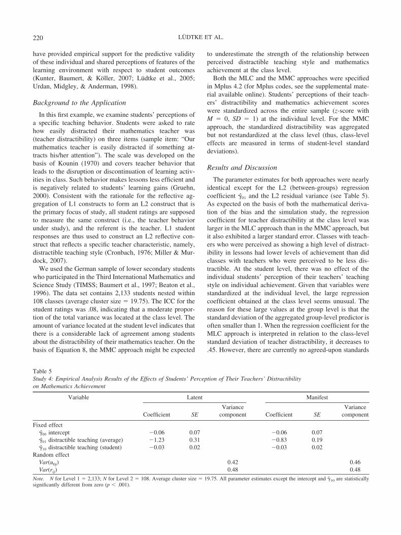
have provided empirical support for the predictive validityof these individual and shared perceptions of features of thelearning environment with respect to student outcomes(Kunter, Baumert, & Koller, 2007; Ludtke et al., 2005;Urdan, Midgley, & Anderman, 1998).

Background to the Application

In this first example, we examine students’ perceptions ofa specific teaching behavior. Students were asked to ratehow easily distracted their mathematics teacher was(teacher distractibility) on three items (sample item: “Ourmathematics teacher is easily distracted if something at-tracts his/her attention”). The scale was developed on thebasis of Kounin (1970) and covers teacher behavior thatleads to the disruption or discontinuation of learning activ-ities in class. Such behavior makes lessons less efficient andis negatively related to students’ learning gains (Gruehn,2000). Consistent with the rationale for the reflective ag-gregation of L1 constructs to form an L2 construct that isthe primary focus of study, all student ratings are supposedto measure the same construct (i.e., the teacher behaviorunder study), and the referent is the teacher. L1 studentresponses are thus used to construct an L2 reflective con-struct that reflects a specific teacher characteristic, namely,distractible teaching style (Cronbach, 1976; Miller & Mur-dock, 2007).

We used the German sample of lower secondary studentswho participated in the Third International Mathematics andScience Study (TIMSS; Baumert et al., 1997; Beaton et al.,1996). The data set contains 2,133 students nested within108 classes (average cluster size � 19.75). The ICC for thestudent ratings was .08, indicating that a moderate propor-tion of the total variance was located at the class level. Theamount of variance located at the student level indicates thatthere is a considerable lack of agreement among studentsabout the distractibility of their mathematics teacher. On thebasis of Equation 8, the MMC approach might be expected

to underestimate the strength of the relationship betweenperceived distractible teaching style and mathematicsachievement at the class level.

Both the MLC and the MMC approaches were specifiedin Mplus 4.2 (for Mplus codes, see the supplemental mate-rial available online). Students’ perceptions of their teach-ers’ distractibility and mathematics achievement scoreswere standardized across the entire sample (z-score withM � 0, SD � 1) at the individual level. For the MMCapproach, the standardized distractibility was aggregatedbut not restandardized at the class level (thus, class-leveleffects are measured in terms of student-level standarddeviations).


The parameter estimates for both approaches were nearlyidentical except for the L2 (between-groups) regressioncoefficient �01 and the L2 residual variance (see Table 5).As expected on the basis of both the mathematical deriva-tion of the bias and the simulation study, the regressioncoefficient for teacher distractibility at the class level waslarger in the MLC approach than in the MMC approach, butit also exhibited a larger standard error. Classes with teach-ers who were perceived as showing a high level of distract-ibility in lessons had lower levels of achievement than didclasses with teachers who were perceived to be less dis-tractible. At the student level, there was no effect of theindividual students’ perception of their teachers’ teachingstyle on individual achievement. Given that variables werestandardized at the individual level, the large regressioncoefficient obtained at the class level seems unusual. Thereason for these large values at the group level is that thestandard deviation of the aggregated group-level predictor isoften smaller than 1. When the regression coefficient for theMLC approach is interpreted in relation to the class-levelstandard deviation of teacher distractibility, it decreases to.45. However, there are currently no agreed-upon standards

Table 5Study 4: Empirical Analysis Results of the Effects of Students’ Perception of Their Teachers’ Distractibilityon Mathematics Achievement

Variable Latent Manifest

Coefficient SEVariance

component Coefficient SEVariance

component

Fixed effect�00 intercept �0.06 0.07 �0.06 0.07�01 distractible teaching (average) �1.23 0.31 �0.83 0.19�10 distractible teaching (student) �0.03 0.02 �0.03 0.02

Random effectVar(u0j) 0.42 0.46Var(rij) 0.48 0.48

Note. N for Level 1 � 2,133; N for Level 2 � 108. Average cluster size � 19.75. All parameter estimates except the intercept and �10 are statisticallysignificantly different from zero (p .001).

220 LUDTKE ET AL.

for how to calculate standardized regression coefficients inMLM. Standardization strategies in MLM remain a topic ofresearch (e.g., Raudenbush & Bryk, 2002).

Students’ ratings of their teachers’ behavior seem to be agood example of an L2 reflective construct where the ratio-nale of the MLC approach is appropriate. In this example,the main purpose of the L2 measurements is to assess an L2group-level construct—the behavior of a particular teacheras perceived by his or her students. In his seminal paper onmultilevel issues in educational research, Cronbach (1976)was very clear about the role of students’ perceptions inassessing aspects of the learning environment. In a discus-sion of the Learning Environment Inventory (LEI), he ar-gued that

The purpose of the LEI is to identify differences among class-rooms. For it, then, studies of scale homogeneity or scale inter-correlation should be carried out with the classroom group asunit of analysis. Studying individuals as perceivers within theclassrooms could be interesting, but is a problem quite separatefrom the measurement of environments. (p. 918)

From this point of view, it is reasonable to correct forfactors that impinge the measurement of that class-levelconstruct. In the MLC approach, the restriction to smallsamples of students within classes and disagreement amongstudents are taken into account when estimating the effect ofaggregated student ratings on achievement.

Study 5: School-Average SES—A Contextual EffectAnalysis of a Formative L2 Construct

Educational researchers believe that a student’s perfor-mance in school is affected by the characteristics of his orher fellow students (Marsh, Kong, & Hau, 2000; Willms,1985). For example, several researchers have posited thataggregated school SES or mean ability affects individualstudent outcomes (e.g., student achievement or academicself-concept), even after controlling for the individual ef-fects of these L1 constructs—a contextual effect. Rauden-

bush and Bryk (2002, p. 139) define such a contextual effectto exist “when the aggregate of a person-level characteristic,X� •j, is related to the outcome, Yij, even after controlling forthe effect of the individual characteristic, Xij.”

Background to the Application

In the present example, individual students’ SES is usedto assess the effect of school-average SES on reading liter-acy after controlling for individual SES, drawing on datafrom the German sample (Baumert et al., 2002) of theProgramme for International Student Achievement (PISA)2000 study (Organisation for Economic Co-operation andDevelopment, 2001). The analyses are based on 4,460 stu-dents in 189 schools, giving a mean of 23.6 students perschool. Note that the PISA study sampled 15-year-old stu-dents from schools rather than classes. Hence, in contrast toStudy 4, where the L2 groups were classes, the presentexample focused on the school at Level 2 (meaning that thesampling ratio is much lower). The ICC for SES was .22,indicating that a substantial amount of the variance in stu-dents’ SES was located at the school level.


The results for both manifest and latent models are re-ported in Table 6. SES and reading scores were standardized(z-score with M � 0, SD � 1) at the individual level. For theMMC approach, the standardized SES was aggregated butnot restandardized at the school level. As expected, thedifferences between the two approaches in the parametersbased on student-level data were negligible. The effect ofstudents’ SES �10 on reading achievement, the L1 residual,and the intercept �00 were almost the same. In contrast,estimates at the school level differed across the two ap-proaches. As expected on the basis of Equation 8, the effectof school-average SES was higher in the MLC approach,which corrects for unreliability of the school-average SESscores. Because we group-centered the L1 predictor vari-

Table 6Study 5: Empirical Analysis Results of the Effects of Socioeconomic Status (SES) on Reading Achievement

Variable

Latent Manifest

Coefficient SEVariance

component Coefficient SEVariance

component

Fixed effect�00 intercept �0.01 0.03 �0.02 0.03�01 SES (average) 1.52 0.06 1.29 0.06�10 SES (student) 0.10 0.01 0.10 0.01

Random effectVar(u0j) 0.08 0.15Var(rij) 0.43 0.43

Note. N for Level 1 � 4,460; N for Level 2 � 189. Average cluster size � 23.6. All parameter estimates except the intercept are statistically significantlydifferent from zero (p .001).


able, the compositional effect was determined by subtract-ing the within-school regression coefficient from the be-tween-schools regression coefficient: �01 � �10 (e.g.,Raudenbush & Bryk, 2002). We obtained a compositionaleffect of 1.42 for the MLC approach and 1.19 for the MMCapproach. The contextual effect can be interpreted as thedifference expected in reading literacy between two stu-dents with the same individual SES who attend schoolsdiffering by one unit in mean SES. One unit in mean SEScorresponds to one standard deviation at the individual levelmetric because the aggregated individual SES score werenot restandardized. Similarly, when the regression coeffi-cients at the school level are interpreted in relation to theschool-level standard deviation of SES, they decrease inabsolute size. For instance, the regression coefficient for theMLC decreases to 0.71 when interpreted in relation to theschool-level standard deviation. Again, this demonstratesthat the magnitude of the parameter estimates is very sen-sitive to the different standardization strategies.

The central question now is whether we can justifiablycorrect for unreliability based on the MLC approach inthe present example. In contrast to Study 4, where stu-dents’ responses serve as reflective indicators of the L2construct (each student provides a single fallible estimateof the teacher’s distractibility), in Study 5 student re-sponses reflect the L1 construct SES. Variability in indi-vidual student levels of SES in a given school clearlyreflects systematic true score variation in a well-definedL1 construct in which the referent is the individual stu-dent (consistent with the formative approach to aggrega-tion). Hence, it does not seem appropriate to assume areflective aggregation process for school-average SES.However, another reason for choosing a MLC approachmight be a low sampling ratio. On average, 23.6 studentswere sampled from each school in the present example.Assuming an average school size of 500, only 5% of thepupils from each school were sampled. Given such a lowsampling ratio in connection with a potentially very largenumber of L1 units within each L2 unit, application ofthe MLC approach may be justified. On the basis of theseassumptions, one can even go further and use the resultsof the simulation study to infer the direction of the bias.For instance, given these assumptions, in the presentexample a researcher can infer that the true value for thecontextual effect of average SES is expected to be closerto the estimate of the MLC approach than to the estimateof the MMC approach (see Table 4A). However, as thisexample shows, the choice of the analysis model (MLCor MMC approach) is very sensitive to the assumptionsmade about the underlying population sampling model.For instance, if classes (with ns of approximately 25) andnot schools were chosen as L2 units and the samplingratio approached 1.0, we would have more confidence inthe MMC approach. For a formative process in which the

sampling ratio is small or moderate, our simulation re-sults might provide preliminary evidence about the rela-tive size (and direction) of biases under the manifest andlatent approaches. Resolving this problem is clearly be-yond the scope of this study. It is, however, importantthat applied researchers are aware of the problem, whichdoes not seem to have been clearly demonstrated inprevious research.

Discussion

Multilevel analyses are frequently used to estimate theeffects of group-level (L2) constructs in the social sciences.When using aggregated individual data to assess an L2construct within the MMC approach, however, the observedgroup mean might not be a reliable measure of the unob-served, latent group characteristic. We compared two ap-proaches to the analysis of contextual models: a new MLCapproach that corrects for the unreliable assessment of thelatent group mean when estimating MLMs and the tradi-tional MMC approach, which relies on manifest groupmeans that are assumed to be perfectly reliable.

Statistical Considerations

By means of mathematical derivation, we showed that theMMC approach results in biased estimates of contextualeffects for reflective aggregations of L1 constructs, partic-ularly when the ICC and L1 sample sizes within groups aresmall. This result was confirmed by a simulation study,which also showed that the MLC approach is generallyunbiased. Although the contextual effects estimated withinthe MLC approach were larger, they were also substantiallymore variable in certain data constellations (e.g., smallnumber of L2 groups, small ICCs, and small n) than thoseobtained using the traditional MMC approach. Indeed, dueto this trade-off, the results of Study 4 suggested that thelikelihood of obtaining statistically significant results wassimilar for both approaches. Although this article clearlydoes not provide sufficient evidence to suggest that thisresult will generalize more broadly, it is a relevant consid-eration for further research. More generally, because thecontextual effect estimates are so variable within the MLCapproach, results based on a given sample may deviatesubstantially from the true population parameter—as can bedemonstrated by a simple inspection of the standard error.

What are the consequences of these mixed findings for thestatistical properties of the estimator of the contextual effectin cases of reflective aggregation? The MMC approach isused almost exclusively in research practice. Our resultssuggest that for the single predictor case at least the sizes ofcontextual effects published are likely to be conservative.Although the new MLC approach is unbiased, the largesampling variability in certain data constellations (e.g.,

222 LUDTKE ET AL.

small number of L2 groups, small ICCs, and small n)suggests that it should be applied only very cautiously insuch cases. Although asymptotically the MLC approachprovides the most efficient and consistent estimator of thecontextual effect and is thus asymptotically superior to theMMC approach, the results of our simulation study suggestthat large numbers of L2 groups (K) may be needed forthese asymptotic properties to hold. Particularly for studieswhere the number of L2 groups and the number of L1 caseswithin each group are modest, the latent variable approachcan be recommended only when the ICC is very large.

We also compared the MLC approach to the two-stagelatent variable approach for L2 reflective constructs pro-posed by Croon and van Veldhoven (2007). Consistent withtheir speculations, our simulation study showed that the twoapproaches yielded very similar results, except under thecondition with small sample sizes at both L1 and L2 and alow ICC. For this data constellation, the FIML MLC ap-proach outperformed the two-stage approach. Because thetwo-stage approach is only a limited information approach,the FIML implementation should be generally preferred.Although it was not a focus of our study, we also note thatthe potentially cumbersome two-stage approach to estimat-ing standard errors requires further consideration. Whendiscussing critical issues for future research in multilevellatent variable modeling, Croon and van Veldhoven (2007,p. 55) emphasized that “efforts should be made to developa reliable numerical and generally applicable procedure thatyields the full information maximum likelihood estimates ofthe model parameters.” Mplus provides such a flexiblelatent variable model that integrates several different anal-ysis models within a unified MLM framework (L. K. Mu-then & Muthen, 2007). Hence, we recommend that theone-step approach demonstrated here be used instead of thetwo-stage approach.

Another even simpler approach (related to the Croon &van Veldhoven, 2007, two-stage approach) would be toestimate the reliability of the group mean via Equation 6 andthen to correct the estimated regression coefficient for theunreliability of the group mean (see Grilli & Rampichini,2007). To this end, the well-known correction for attenua-tion formula can be used to adjust the between-groups

regression coefficient by multiplying it by1

Rel�X� j��

�2 � 2/n

�2 .

This disattenuation approach thus consists of two steps.First, the MMC model is specified to estimate the between-groups regression coefficient. Second, the estimated be-tween-groups regression coefficient is corrected for unreli-ability by the attenuation formula. In other words, the MMCapproach is used to implement an MLC approach. A majordrawback of that approach is that it is well defined only forbalanced group sizes. However, even if the group sizes varymoderately, it may be acceptable to use the mean group size(see Snijders & Bosker, 1999, for a discussion of different

adjustment formulas). In addition, the standard error of theregression coefficient needs to be adjusted when applyingthe disattenuation approach (e.g., using a bootstrappingprocedure; see Carpenter, Goldstein, & Rasbash, 2003).Further research should evaluate how this disattenuationapproach is related to the FIML implementation of the MLCapproach as well as to the MMC approach for balanced andunbalanced group sizes. Although it may be premature torecommend that this disattenuation approach be used rou-tinely, it does provide the applied researcher with an initialindication of the size of the bias that might be expectedwithin the MMC approach when the MLC approach isappropriate. However, further investigation of the approachis required, particularly for small sample sizes.

Another important application of the MLC approach iswhen the true value of an L2 formative construct is un-known because the entire cluster has not been sampled. Inthis case, the MLC approach is used to control for a lowsampling ratio and the limited reliability of the L2 formativeconstruct. In Study 3, we tested the MLC approach’s suit-ability for adjusting for the effect of a small sampling ratiofrom a finite population. The results showed that, when thefinite sample size of the L2 units is at least moderate (e.g.,100) and the sampling ratio is low (e.g., 20%; 20 cases froma finite population of 100), the MLC approach outperformedthe MMC approach in terms of both bias and RMSE.Critically, however, the bias associated with the two ap-proaches was in opposite directions. Importantly, for for-mative aggregations, a sampling ratio tending to 0 corre-sponds with the assumptions of the MLC approach, whereasa sampling ratio of 1 corresponds with the assumptions ofthe MMC approach.

The relative sizes of the counterbalancing biases associ-ated with the two approaches varied systematically withsample size and sampling ratio. When the number of L1cases within each L2 group is sufficiently large, the manifestand latent approaches give similar results (because L2 un-reliability is negligible). However, when the sampling ratioand sample size are both small, and the two approaches arethus likely to give very different results, the only conclusionthat the applied researcher can make with confidence is thatthe true value is on average somewhere between the resultsof the MMC and the MLC approaches. Hence, the mostreasonable recommendation is to use both approaches todetermine whether their results point to substantively dif-ferent conclusions. If so, conclusions must be made withcaution.

What are the consequences of these findings for applyingthe MLC approach to group-level constructs based on for-mative aggregation? In research practice, it is often difficultto determine the true cluster sizes because ad hoc samplesare frequently drawn without a sampling scheme. In Study5, for example, there was an average of 23.6 students perschool. If we assume that the average school size is at least


500 students, then the sampling ratio is less than .05. How-ever, the sample was limited to students who were 15 yearsof age, and the average number of 15-year-old students perschool might be just 100. We are not necessarily arguing forthis alternative interpretation, but we use this example toillustrate why the computation of sampling ratio might notbe straightforward. Furthermore, the true cluster sizes arelikely to vary, perhaps substantially, across different L2groups. Thus, further research is needed to study the effectof varying finite sample sizes of the L2 clusters on theestimator of the contextual effect based on L2 formativeconstructs. Although our simulation results do not provide asufficient basis for making detailed recommendations, wewould like to offer the following guidelines (subject tofurther research).

For formative L2 constructs (as in Study 5), the MMCapproach can comfortably be used when the sampling ratioapproaches 1.0. Even when the sampling ratio is moderate(at least .5), the MMC approach seems to provide relativelyunbiased estimates as long as the sample size and ICC arelarge. The MLC approach should be considered instead ofthe MMC approach when the sampling ratio is very smalland the numbers of L2 groups and L1 cases in each L2group are large. In all other cases, the applied researchershould apply both the latent and manifest approaches andcompare the results of each. If the results of the two ap-proaches differ substantively, the applied researcher shouldbe cautious in drawing any conclusions. Because theserecommendations are not entirely satisfactory in providingclear-cut advice, this is an area in which more research isneeded. We also note that there may be applications wherethe true population mean for each L2 group is known (e.g.,based on information external to the study such as genderratio of a school), although only a sample of participants isconsidered. In this special case, it would be appropriate touse the known true population mean for each group (insteadof the sample mean based on data actually collected) and tointerpret the sampling ratio in relation to this L2 construct asbeing 100%. Hence, for formative L2 constructs in whichthe true (population) sample mean is known for each L2group, we recommend that the MMC is always appropriateand should be used instead of the MLC approach describedhere.

For reflective L2 constructs, the researcher should alwaysuse the MLC approach in preference to the MMC ap-proach—even when the apparent sampling ratio is verylarge. The rationale for this recommendation, as for thedomain sampling rationale in the classical approach to mea-surement, is that there is a potentially infinite number of L1indicators that could be sampled. There are, however, im-portant qualifications to this recommendation. When thenumber of groups, the number of cases within each group,and the ICC are all modest, the contextual effect estimatesfor the MLC approach are—because of their larger vari-

ability—less accurate than those of the MMC approach.However, we cannot recommend the MMC approach be-cause the parameter estimates are likely to be very nega-tively biased and the apparently small standard errors arelikely to substantially underestimate sampling variability (atleast in terms of making population inferences). Rather, werecommend that the results of contextual effects studies forreflective L2 constructs based on small ns at L1 and, inparticular, small numbers of L2 groups be interpreted verycautiously unless the ICCs are substantial.

Theoretical Considerations

In multilevel studies, group-level constructs are oftenconstructed by aggregating individual data at the grouplevel. The theoretical rationale for the aggregation processmay differ. In this article, we distinguish two quite differentaggregation processes—reflective and formative aggrega-tion—that represent opposite ends of a continuum.

At the reflective aggregation end, the aggregation processassumes an isomorphic relationship between the individual-level data and the group-level construct. In other words, ageneric group-level construct is assumed to be measured bythe corresponding constructs at the individual level. A typ-ical research paradigm was presented in Study 4, in whichL1 students’ responses were treated as observers of their L2teacher’s behavior and the referent was the L2 teacher.Ideally, each student would assign the same rating, such thatthe responses of students in the same class would be inter-changeable. Because the L1 perceptions of each studentwere designed to measure the same L2 construct, variationwithin each class can be regarded as L2 unreliability (Cron-bach, 1976; Van Mierlo, Vermunt, & Rutte, 2008). Thissituation is analogous to typical assumptions in test con-struction, in which differences between multiple items areassumed to reflect measurement error that varies as a func-tion of the number of items and the size of correlationsamong items. Further examples of group-level constructsthat rely on this aggregation process are multiple L1 asses-sors’ evaluations of the L2 quality of grant proposals (Ja-yasinghe et al., 2003), L1 students’ evaluations of L2 teach-ing effectiveness (Marsh, 1987, 2007), and multipleinterchangeable L1 markers assessing the quality of studentessays. In each of these situations in which the referent is agroup-level construct, the reflective aggregation of L1 con-structs to form L2 constructs and the application of theMLC approach seem reasonable.

At the formative aggregation end of the continuum, theaggregation process assumes that the group-level variable ismerely an index of a well-defined L1 construct that is aggre-gated to the L2 group level. In other words, the aggregation isnot based on multiple interchangeable observations of a singleentity but on different characteristics associated with discrete(noninterchangeable) individuals. In fact, under appropriate

224 LUDTKE ET AL.

circumstances (high levels of reliability at L1 and large num-bers of L1 cases within each L2 group or a sampling ratio thatapproaches 1.0), it is reasonable to argue that nearly all of thewithin-group variability reflects true score differences amongdifferent individuals within each group. As such, L2 unreli-ability becomes trivial in size and, perhaps, ignorable (consis-tent with the MMC approach). Particularly when the main aimof a construct is to reflect individual differences at L1 (e.g.,academic achievement, SES, individual demographic charac-teristics such as race, age, and gender) and the referent is an L1construct, the level of interrater agreement associated with theaggregated L2 construct may be of no consequence to con-struct validity at L1 (Bliese, 2000). This situation was demon-strated in Study 5, in which school-average SES was deter-mined by aggregating individual-level (L1) student SES.

Limitations of the Manifest and Latent Approaches:Directions for Further Research

As formulated in this article, both the manifest and thelatent covariate approaches begin with manifest scale scoresat L1, largely ignoring the potential to estimate and controlfor measurement error at L1—even when L1 measures arebased on multiple indicators. Under appropriate circum-stances, the integration of multiple L1 indicators into theanalyses would allow researchers using either of the twoapproaches to differentiate between L1 measurement errorand L2 unreliability due to sampling error associated withthe aggregation process in moving from L1 to L2 aggrega-tions. This would be particularly valuable for the MMCapproach, offering researchers a way to estimate L2 unre-liability in L2 formative measures (see Kline, 2005, fordiscussion of how to take account of measurement error inobserved exogenous variables). Furthermore, low reliabilityof individual measures can give the appearance of substan-tial estimates of group-level contextual effects. However,these estimates are biased because the aggregate measure ismore reliable and “mops up” variance that would be ex-plained at the individual level with more reliable mea-sures—the so-called phantom effect or contextual fallacy(Harker & Tymms, 2004; see also Ludtke, Robitzsch, &Koller, 2002). Historically, limitations in statistical softwareposed intractable problems in integrating confirmatory fac-tor analysis/SEM and MLM models (e.g., Mehta & Neale,2005; B. O. Muthen, 1991). However, even with conven-tional MLM programs that do not explicitly incorporatemultiple indicators of each L1 construct, it is possible toincorporate information about L1 measurement error (e.g.,Goldstein, 2003; Raudenbush & Bryk, 2002). More sophis-ticated statistical packages are increasingly providing ap-plied researchers with added flexibility to incorporate mul-tiple indicators at L1 while addressing the multilevelstructure of their data.

In the present article, we looked at models in which only

the intercepts were allowed to vary (random-intercept mod-els). However, in research practice models that allow slopesto vary between L2 units are of great interest (random-slopemodels). For instance, following our application in Study 5,the relationship between SES and reading achievementcould be different in high and low SES schools (see alsoExample 9.10 in L. K. Muthen & Muthen, 2007). Furtherresearch is needed to investigate the behavior of the MLCand MMC approaches when identifying these cross-levelinteractions.

Implicit in our presentation of the MLC approach for L2reflective measures is the assumption that L1 individualscan be regarded as indicators and that these indicators aredrawn from a population of infinite potential indicators torepresent each L2 group, analogous to assumptions made inthe domain sampling approach to classical measurementtheory. From this perspective, sampling ratio is not a criticalconcern for reflective L2 measures, although concerns abouthaving adequate numbers of L1 cases in each L2 group arestill relevant. Although the correction for unreliability in L2aggregates in the MLC approach is generally appropriateunder the assumption that it is at least hypothetically pos-sible to have an infinitely large sample size, this assumptionmay be questionable in situations in which it is not feasibleto have a large number of L1 cases for each L2 group.

In the MLC procedure, ICCs are an index of interrateragreement and one basis for the determination of L2 reli-ability. With an ICC � 0, which implies a reliability of zero,correction for unreliability becomes problematic. The samewould apply to reliability estimates based on multiple itemsin the classical approach to measurement; this is not an issuethat is idiosyncratic to our new approach. Hence, it is notsurprising that the largest difference between the MMCapproach (that ignores unreliability) and the MLC approach(that corrects for unreliability) is when reliability is verylow. Thus, it is important that researchers routinely providean estimate for the ICC when applying the MLC approachand, if the ICC is close to zero, justify the appropriatenessof subsequent analyses and their interpretations. Furtherresearch on the most appropriate estimation procedure andinterpretation of results based on very small ICCs is war-ranted.

Conclusion

The simultaneous investigation of individual and groupeffects is one of the basic features of MLMs. In researchpractice, the L2 group characteristics are often measured byaggregation from L1 individual measures. Two approachesthat differ in their treatment of the aggregated group-levelconstruct were compared. Whereas the MLC approach cor-rects for the unreliable assessment of the latent group meanwhen estimating MLMs, the MMC approach relies solelyon the observed group mean that is assumed to be measured


with no L2 unreliability. We argue that the appropriatenessof either of these approaches depends on the research ques-tion and the nature of the L2 construct under study. If ageneric group-level construct is assessed through a reflec-tive aggregation of L1 measures to form the L2 construct,then the MLC approach is appropriate and offers manyadvantages as long as minimal standards are met. However,when the aggregated variable is a formative summary of theobservations at the individual level (e.g., school-averageSES), the assumptions made by the MLC approach areappropriate only when the sampling ratio is small. In re-search practice, the distinction between group-level vari-ables based on reflective and formative aggregation is notusually so clear cut, and it is easy to imagine situations inwhich the theoretical status of the group-level construct isambiguous and the calculation of the sampling ratio is notstraightforward. Hence, it might be useful to analyze thesensitivity of empirical results to both approaches. In con-clusion, although the latent covariate approach demon-strated here has wide applicability in relation to a seriouslimitation of existing research, the appropriateness of itsapplication varies depending on the nature of the data, thenumber of L2 groups, the number of cases within eachgroup, and the sampling ratio.

References

Anderman, E. M. (2002). School effects on psychological out-comes during adolescence. Journal of Educational Psychology,94, 795–809.

Asparouhov, T., & Muthen, B. (2003). Full-information maxi-mum-likelihood estimation of general two-level latent variablemodels with missing data (Tech. report). Los Angeles: Muthen& Muthen.

Asparouhov, T., & Muthen, B. (2006). Constructing covariates inmultilevel regression. Mplus Web Notes: No. 11. Retrieved fromhttp://www.statmodel.com/download/webnotes/webnote11.pdf

Bauer, D. J., Preacher, K. J., & Gil, K. M. (2006). Conceptualizingand testing random indirect effects and moderated mediation inmultilevel models: New procedures and recommendations. Psy-chological Methods, 11, 142–163.

Baumert, J., Artelt, C., Klieme, E., Neubrand, M., Prenzel, M.,Schiefele, U., et al. (Eds.). (2002). PISA 2000: Die Lander derBundesrepublik Deutschland im Vergleich [PISA 2000: A com-parison of the German states]. Opladen, Germany: Leske &Budrich.

Baumert, J., Lehmann, R. H., Lehrke, M., Schmitz, B., Clausen,M., Hosenfeld, I., et al. (1997). TIMSS: Mathematisch-Natur-wissenschaftlicher Unterricht im internationalen Vergleich[TIMSS: Mathematics and science instruction in an interna-tional comparison]. Opladen, Germany: Leske & Budrich.

Beaton, A. E., Mullis, I. V. S., Martin, M. O., Gonzales, E. J.,Kelly, D. L., & Smith, T. A. (1996). Mathematics achievement

in the middle school years: IEA’s Third International Mathe-matics and Science Study. Chestnut Hill, MA: Boston College.

Blakely, T. A., & Woodward, A. J. (2000). Ecological effects inmulti-level studies. Journal of Epidemiological Health, 54,367–374.

Bliese, P. D. (2000). Within-group agreement, non-independence,and reliability: Implications for data aggregation and analysis. InK. J. Klein & S. W. Kozlowski (Eds.), Multilevel theory, re-search, and methods in organizations (pp. 349–381). San Fran-cisco: Jossey-Bass.

Bliese, P. D., Chan, D., & Ployhart, R. E. (2007). Multilevelmethods: Future directions in measurement, longitudinal analy-ses, and nonnormal outcomes. Organizational Research Meth-ods, 10, 551–563.

Bollen, K., & Lennox, R. (1991). Conventional wisdom on mea-surement: A structural equation perspective. Psychological Bul-letin, 110, 305–314.

Boyd, L., & Iverson, G. (1979). Contextual analysis: Concepts andstatistical techniques. Belmont, CA: Wadsworth.

Carpenter, J. R., Goldstein, H., & Rasbash, J. (2003). A novelbootstrap procedure for assessing the relationship between classsize and achievement. Applied Statistics, 52, 431–443.

Carroll, R. J., Ruppert, D., & Stefanski, L. A. (1995). Measure-ment error in nonlinear models. London: Chapman & Hall/CRC.

Chan, D. (1998). Functional relations among constructs in thesame content domain at different levels of analysis: A typologyof composition models. Journal of Applied Psychology, 83,234–246.

Chen, G., Bliese, P. D., & Mathieu, J. E. (2005). Conceptualframework and statistical procedures for delineating and testingmultilevel theories of homology. Organizational ResearchMethods, 8, 375–409.

Cronbach, L. J. (1976). Research on classrooms and schools:Formulations of questions, design and analysis. Stanford, CA:Stanford Evaluation Consortium.

Croon, M. A., & van Veldhoven, M. J. P. M. (2007). Predictinggroup-level variables from variables measured at the individuallevel: A latent variable multilevel model. Psychological Meth-ods, 12, 45–57.

Davis, J. A. (1966). The campus as a frog pond: An application ofthe theory of relative deprivation to career decisions of collegemen. American Journal of Sociology, 72, 17–31.

Edwards, J. R., & Bagozzi, R. P. (2000). On the nature anddirection of relationships between constructs and measures.Psychological Methods, 5, 155–174.

Firebaugh, G. (1978). A rule for inferring individual-level rela-tionships from aggregate data. American Sociological Review,43, 557–572.

Goldstein, H. (1987). Multilevel models in educational and socialresearch. London: Griffin.

Goldstein, H. (2003). Multilevel statistical models. London: Ar-nold.

226 LUDTKE ET AL.

Grilli, L., & Rampichini, C. (2007). Endogeneity issues in multi-level linear models. Unpublished manuscript.

Gruehn, S. (2000). Unterricht und schulisches Lernen: Schuler alsQuellen der Unterrichtsbeschreibung [Instruction and learningin school: Students as sources of information]. Munster, Ger-many: Waxmann.

Harker, R., & Tymms, P. (2004). The effects of student composi-tion on school outcomes. School Effectiveness and School Im-provement, 15, 177–199.

Howell, R. D., Breivik, E., & Wilcox, J. B. (2007). Reconsideringformative measurement. Psychological Methods, 12, 205–218.

Hox, J. J. (2002). Multilevel analysis: Techniques and applica-tions. Mahwah, NJ: Erlbaum.

Iverson, G. R. (1991). Contextual analysis (Sage University PaperSeries on Quantitative Applications in the Social Sciences No.07–081). Newbury Park, CA: Sage.

James, L. R. (1982). Aggregation bias in estimates of perceptualagreement. Journal of Applied Psychology, 67, 219–229.

Jayasinghe, U. W., Marsh, H. W., & Bond, N. (2003). A multilevelcross-classified modelling approach to peer review of grantproposals: The effects of assessor and researcher attributes onassessor ratings. Journal of the Royal Statistical Society SeriesA: Statistics in Society, 166, 279–300.

Kenny, D. A., & La Voie, L. (1985). Separating individual andgroup effects. Journal of Personality and Social Psychology, 48,339–348.

Kenny, D. A., Mannetti, L., Pierro, A., Livi, S., & Kashy, D. A.(2002). The statistical analysis of data from small groups. Jour-nal of Personality and Social Psychology, 83, 126–137.

Kline, R. B. (2005). Principles and practice of structural equationmodeling (2nd ed.). New York: Guilford Press.

Kounin, J. S. (1970). Discipline and group management in class-rooms. New York: Holt, Rinehart & Winston.

Kozlowski, S. W. J., & Klein, K. J. (2000). A multilevel approachto theory and research in organizations: Contextual, temporal,and emergent processes. In K. J. Klein & S. W. J. Kozlowski(Eds.), Multilevel theory, research, and methods in organiza-tions: Foundations, extensions, and new directions (pp. 3–90).San Francisco: Jossey-Bass.

Kreft, I. G. G., de Leeuw, J., & Aiken, L. S. (1995). The effect ofdifferent forms of centering in hierarchical linear models. Mul-tivariate Behavioral Research, 30, 1–21.

Kunter, M., Baumert, J., & Koller, O. (2007). Effective classroommanagement and the development of subject-related interest.Learning and Instruction, 17, 494–509.

Lee, S.-Y., & Poon, W.-Y. (1998). Analysis of two-level structuralequation models via EM type algorithms. Statistica Sinica, 8,749–766.

Lord, F. R., & Novick, M. (1968). Statistical theories of mentaltest scores. Reading, MA: Addison-Wesley.

Ludtke, O., Koller, O., Marsh, H. W., & Trautwein, U. (2005).Teacher frame of reference and the big-fish–little-pond effect.Contemporary Educational Psychology, 30, 263–285.

Ludtke, O., Robitzsch, A., & Koller, O. (2002). Statistische Arte-

fakte bei Kontexteffekten in der padagogisch-psychologischenForschung [Statistical artifacts in educational studies on contexteffects]. German Journal of Educational Psychology, 16, 217–231.

Ludtke, O., Trautwein, U., Kunter, M., & Baumert, J. (2006).Reliability and agreement of student ratings of the classroomenvironment: A reanalysis of TIMSS data. Learning Environ-ments Research, 9, 215–230.

Maas, C. J. M., & Hox, J. J. (2005). Sufficient sample sizes formultilevel modeling. Methodology, 1, 86–92.

Marsh, H. W. (1987). Students’ evaluations of university teaching:Research findings, methodological issues, and directions forfuture research. International Journal of Educational Research,11, 253–388.

Marsh, H. W. (2007). Students’ evaluations of university teaching:A multidimensional perspective. In R. P. Perry & J. C. Smart(Eds.), The scholarship of teaching and learning in highereducation: An evidence-based perspective (pp. 319–384). NewYork: Springer.

Marsh, H. W., & Ball, S. (1981). The interjudgmental reliability ofreviews for the Journal of Educational Psychology. Journal ofEducational Psychology, 18, 872–880.

Marsh, H. W., & Hau, K.-T. (2003). Big-fish–little-pond effect onacademic self-concept: A cross-cultural (26 country) test of thenegative effects of academically selective schools. AmericanPsychologist, 58, 364–376.

Marsh, H. W., Kong, C.-K., & Hau, K.-T. (2000). Longitudinalmultilevel models of the big-fish–little-pond effect on academicself-concept: Counterbalancing contrast and reflected-glory ef-fects in Hong Kong schools. Journal of Personality and SocialPsychology, 78, 337–349.

McCulloch, C. E., & Searle, S. R. (2001). Generalized, linear, andmixed models. New York: Wiley.

Mehta, P. D., & Neale, M. C. (2005). People are variables too:Multilevel structural equations modeling. Psychological Meth-ods, 10, 259–284.

Miller, A. D., & Murdock, T. B. (2007). Modeling latent truescores to determine the utility of aggregate student perceptionsas classroom indicators in HLM: The case of classroom goalstructures. Contemporary Educational Psychology, 32, 83–104.

Muthen, B. O. (1989). Latent variable modeling in heterogeneouspopulations. Psychometrika, 54, 557–585.

Muthen, B. O. (1991). Multilevel factor analysis of class andstudent achievement components. Journal of Educational Mea-surement, 28, 338–354.

Muthen, B. O. (2002). Beyond SEM: General latent variablemodeling. Behaviormetrika, 29, 81–117.

Muthen, L. K., & Muthen, B. O. (2007). Mplus user’s guide. LosAngeles: Muthen & Muthen.

Nunnally, J. C., & Bernstein, I. H. (1994). Psychometric theory(3rd ed.). New York: McGraw-Hill.

O’Brien, R. M. (1990). Estimating the reliability of aggregate-level variables based on individual-level characteristics. Socio-logical Methods and Research, 18, 473–504.


Organisation for Economic Co-operation and Development.(2001). Knowledge and skills for life. First results from theOECD Programme for International Student Assessment (PISA)2000. Paris: Author.

Papaioannou, A., Marsh, H. W., & Theodorakis, Y. (2004). Amultilevel approach to motivational climate in physical educa-tion and sport settings: An individual or a group level construct?Journal of Sport and Exercise Psychology, 26, 90–118.

Rabe-Hesketh, S., Skrondal, A., & Pickles, A. (2004). Generalizedmultilevel structural equation modeling. Psychometrika, 69,167–190.

Raudenbush, S. W., & Bryk, A. S. (2002). Hierarchical linearmodels (2nd ed.). Thousand Oaks, CA: Sage.

Raudenbush, S. W., Rowan, B., & Kang, S. J. (1991). A multi-level, multivariate model for studying school climate with esti-mation via the EM algorithm and application to U.S. high-school data. Journal of Educational Statistics, 16, 295–330.

Raykov, T. (2007). Longitudinal analysis with regressions amongrandom effects: A latent variable modeling approach. StructuralEquation Modeling, 14, 146–169.

Ryan, A. M., Gheen, M. H., & Midgley, C. (1998). Why do somestudents avoid asking for help? An examination of the interplayamong students’ academic efficacy, teachers’ social–emotionalrole, and the classroom goal structure. Journal of EducationalPsychology, 90, 528–535.

Schmidt, W. H. (1969). Covariance structure analysis of the

multivariate random effects model. Unpublished doctoral dis-sertation, University of Chicago.

Searle, S. R., Casella, G., & McCulloch, C. E. (1992). Variancecomponents. New York: Wiley.

Seber, G. A. F. (1977). Linear regression analysis. New York:Wiley.

Skrondal, A., & Rabe-Hesketh, S. (2004). Generalized latent vari-able modeling: Multilevel, longitudinal, and structural equationmodels. Boca Raton, FL: Chapman & Hall/CRC.

Snijders, T. A. B., & Bosker, R. J. (1999). Multilevel analysis: Anintroduction to basic and advanced multilevel modeling. Lon-don: Sage.

Urdan, T., Midgley, C., & Anderman, E. M. (1998). The role ofclassroom goal structure in students’ use of self-handicappingstrategies. American Educational Research Journal, 35, 101–122.

Van Mierlo, H., Vermunt, J. K., & Rutte, C. G. (2008). Com-posing group-level constructs from individual-level surveydata. Organizational Research Methods. Advance onlinepublication. Retrieved June 10, 2008. doi:10.1177/10944-28107309322

Willms, D. (1985). The balance thesis: Contextual effects of abilityon pupils’ examination results in Scotland. Oxford Review ofEducation, 11, 33–41.

Wooldridge, J. M. (2002). Econometric analysis of cross sectionand panel data. Cambridge, MA: MIT Press.

Appendix

Derivation of Bias for the Multilevel Manifest Covariate (MMC) Approach

In this Appendix, we derive the bias for the MMC ap-proach. Because we are interested in within-group and be-tween-groups relations, the following population model fortwo variables X and Y will be assumed (see Snijders &Bosker, p. 29):

Xij � �x � Uxj � Rxij

Yij � �y � Uyj � Ryij.

In this model, group (e.g., school) j has specific maineffects Uxj and Uyj for variables X and Y, and the within-group deviations Rxij and Ryij are associated with individual(e.g., student) i. The population means are denoted �x and�y, and it is assumed that the Us and the Rs have populationmeans 0. In addition, the Us and the Rs are independent.

The covariance matrix of X and Y at Level 1 and Level 2can be written as

Level 1 (within) Level 2 (between)

� x2

xy y2 � � �x

2

�xy �y2 � .

We are interested in estimating the following relationship inthe population:

Yij � �y � �withinRxij � �betweenUxj � j � εij.

where �y is the grand mean, �within the within-group regres-sion coefficient, �between the between-groups regression co-efficient, j a group-specific residual, and εij an individual-specific residual. In the group-mean centered case, thefollowing multilevel model would be specified to estimate�within and �within:

Yij � �00 � �10�Xij � X� •j� � �01X� •j � u0j � rij.

Under the assumption of equal group sizes n, X� •j

�1

n�

i�1

n

Xij is the mean for group j. Furthermore, �00,

�10,and �01 denote the estimators for �y, �within, and �be-

tween. The L2 and L1 residuals are given by u0j and rij. Giventhe covariance matrix of X and Y at Level 1 and Level 2, the

228 LUDTKE ET AL.

observed covariance matrix of Yij, Xij � X� •j, and X� •j isdistributed as follows:

Cov� Yij

Xij � X� •j

X� •j

�� y

2 � �y2

xy � �1 � 1/n� x2�1 � 1/n�

�xy � xy/n 0 �x2 � x

2/n� .

As can be seen, the covariances between Yij, Xij � X� •j, andX� •j depend on the common group size as well as on the“true” covariances within and between groups. Employingthe OLS principle and bearing in mind that the predictorsXij � X� •j and X� •j are uncorrelated, the estimator �10 for thewithin-group regression coefficient �within can be obtainedas

�10 �Cov�Yij,Xij � X� •j�

Var�Xij � X� •j��

xy�1 � 1/n�

x2�1 � 1/n�

�xy

x2 � �within.

Now let ICCx ��x

2

�x2 � x

2. denote the ICC for X. The

estimator �01 of the between-groups regression coefficient�between can now be formulated as follows:

�01 �Cov�Yij,X� •j�

Var�X� •j��

�xy � xy/n

�x2 � x

2/n

��xy

�x2 �

�x2

�x2 � x

2/n�

xy/n

x2/n

�x

2/n

�x2 � x

2/n

� �between � �1 �1

n�

�1 � ICCx�

ICCx � �1 � ICCx�/n�

� �within �1

n�

�1 � ICCx�

ICCx � �1 � ICCx�/n.

Thus, the bias on the between level is now computed asfollows:

E��01 � �between�

� ��within � �between� �1

n�

�1 � ICCx�

ICCx � �1 � ICCx�/n.

As can be seen, the bias depends primarily on the proportionof variance in X that is located between groups (ICCx) andon the average group size n. If n3 �, the estimator will beunbiased.

Received August 28, 2007Revision received May 1, 2008

Accepted May 7, 2008 �


The Multilevel Latent Covariate Model: A New, More …The Multilevel Latent Covariate Model: A New,...

Documents

Transcript of The Multilevel Latent Covariate Model: A New, More …The Multilevel Latent Covariate Model: A New,...