The Modeling and Simulation of EV3 Motor Dynamics/67531/metadc862751/m2/1/high... · Lego...

APPROVED: Yan Wan, Major Professor Xinrong Li, Committee Member Shengli Fu, Committee Member and Chair of

the Department of Electrical Engineering

Costas Tsatsoulis, Dean of the College of Engineering

Victor Prybutok, Vice Provost of the Toulouse Graduate School

THE MODELING AND SIMULATION OF EV3 MOTOR DYNAMICS

Roya Norouzi Kandalan

Thesis Prepared for the Degree of

MASTER OF SCIENCE

UNIVERSITY OF NORTH TEXAS

August 2016

Norouzi Kandalan, Roya. The Modeling and Simulation of EV3 Motor Dynamics. Master

of Science (Electrical Engineering), August 2016, 81 pp., 14 tables, 41 figures, 20 numbered

references.

This paper describes a procedure to find the transfer function for the Lego Mindstorms

Ev3. Lego Mindstorms Ev3 can serve as the platform for a system modeling and a controller

design course. It is economical and accessible. It is also very compatible with Matlab and

Simulink. This platform can be used for concepts of modeling, feedback, and controller design.

The main approach in this work focuses on the closed loop instead of open loop. Although this

approach turns the problem into a more complicated puzzle, it reveals more details. In this

work, different techniques have been used, such as time domain, root locus, and least square

estimation. Different tools have also been utilized such as Matlab SISO tool, the Matlab System

Identification tool, and Simulink. These methods and implementations assisted to acquire

different types of transfer functions for the system. By simulating the transfer functions and

comparing them with experimental studies, the matching scores were calculated to decide on

the best transfer function. Finding the finest transfer function for this gadget enables us to

prepare diverse practical undergraduate and graduate curricula.

ii

Copyright 2016

by

Roya Norouzi Kandalan

iii

ACKNOWLEDGMENTS

I would first like to thank my thesis advisor Dr. Yan Wan of the Department of Electrical

Engineering at University of North Texas. The door to Prof. Wan office was always open

whenever I ran into a trouble spot or had a question about my research or writing. She

consistently allowed this paper to be my own work, but steered me in the right direction

whenever she thought I needed it.

I would also like to acknowledge Dr. Fu and Dr. Li of Department of Electrical Engineering

at University of North Texas, as the second readers of this thesis, and I am gratefully indebted

to them for their helpful comments on this thesis.

Finally, I must express my very profound gratitude to my mother who is also my role

model in my life, my family, and friends for providing me with unfailing support and continuous

encouragement throughout my years of study and through the process of researching and

writing this thesis. This accomplishment would not have been possible without them.

iv

TABLE OF CONTENTS

ACKNOWLEDGMENTS ..................................................................................................................... iii

LIST OF TABLES ................................................................................................................................. v

LIST OF FIGURES ............................................................................................................................. vii

CHAPTER 1 INTRODUCTION........ ..................................................................................................... 1

1.1 Lego Mindstorms EV3 ......................................................................................................... 1

1.2 Related Works .................................................................................................................... 3

1.3 Motivation and Contributions ............................................................................................ 5

1.4 Thesis Outline and Organization ........................................................................................ 5

CHAPTER 2 IDENTIFYING THE TRANSFER FUNCTION ..................................................................... 7

2.1 Second Order Transfer Function without Zero ................................................................ 12

2.2 Second Order Transfer Function with One Zero .............................................................. 42

2.3 Third Order Transfer Function without Zero .................................................................... 56

2.4 Third Order Transfer Function with One Zero .................................................................. 64

CHAPTER 3 CONCLUSION .............................................................................................................. 77

REFERENCES .................................................................................................................................. 79

v

LIST OF TABLES

Table 2-1 Matching rate of the different transfer functions with 2 poles and no zero comparing

with the different experiment. ..................................................................................................... 25

Table 2-2 Poles in open loop and closed loop form. ................................................................... 27

Table 2-3 Matching rate of the final transfer functions with 2 poles and no zero comparing with

the different experiment .............................................................................................................. 41

Table 2-4 Matching rate of the different transfer functions with 2 poles and one zero

comparing with the different experiment. ................................................................................... 50

Table 2-5 Poles in open loop and closed loop form. ................................................................... 51

Table 2-6 Matching rate of the final transfer functions with 2 poles and one zero comparing


Table 2-7 Routh Hurwitz for transfer function with three poles and no zero. ............................ 56



Table 2-9 Poles in closed loop form. ............................................................................................ 60

Table 2-11 Matching rate of the final transfer functions with 3 poles and no zero comparing


Table 2-12 Routh Hurwitz for transfer function with 3 poles and one zero. .............................. 65



vi

Table 2-14 Matching rate of the averaged normalized form with 3 poles and one zero

comparing with the different experiment. ................................................................................... 71

Table 2-15 open loop poles and zeros. ........................................................................................ 74

vii

LIST OF FIGURES

Figure 1.1 (a) Lego Mindstorms EV3. (b) Net-gear 1100 Wi-Fi dongle ......................................... 2

Figure 2.1 Open loop system representation. ............................................................................... 7

Figure 2.2 Closed loop system representation. ............................................................................. 8

Figure 2.3 The Simulink representation of Lego Mindstorms EV3 in the circuit. .......................... 9

Figure 2.4 Three sets of real time data for different set-points. ................................................. 11

Figure 2.5 Damping ratio and natural frequency representation in the S plain. ........................ 14

Figure 2.6 The Damping ratio distribution ................................................................................... 15

Figure 2.7 The Natural frequency distribution. ........................................................................... 15

Figure 2.8 Simulated circuit. ........................................................................................................ 16

Figure 2.9 Steady state errors corresponding with the second order system chosen as transfer

function. Dashed line shows the simulation result and the solid line is the real data. ................ 17

Figure 2.10 System model with an integrator. ............................................................................ 21

Figure 2.11 Experimented data vs. simulated data. .................................................................... 22

Figure 2.12 (Data 1): transfer function derived from set point equal to 100, (Data 2):

experimental data for set-point equal to 10. ............................................................................... 24

Figure 2.13 Time domain parameter distribution. ...................................................................... 29

Figure 2.14 System root locus with no gain. ................................................................................ 30

Figure 2.15 Step response of the system with no gain. ............................................................... 31

Figure 2.16 Root locus of the system double real poles. ............................................................. 33

Figure 2.17 Step response of the system double real poles. ....................................................... 33

viii

Figure 2.18 System root locus with time domain requirement specified region. ....................... 35

Figure 2.19 System root locus with time domain requirement satisfied. ................................... 36

Figure 2.20 System step response with time domain requirement satisfied. ............................. 37

Figure 2.21 System step response with time domain requirement satisfied. ............................. 38

Figure 2.22 Normalized averaged experiment vs simulation result. ........................................... 39

Figure 2.23 Simulation data and averaged normalized data. ...................................................... 40

Figure 2.24 Root locus. ................................................................................................................. 40

Figure 2.25 Open loop poles and zero root locus representation. The yellow region is where the

demand is not satisfied. ................................................................................................................ 47

Figure 2.26 Closed loop step response. The yellow region is where the demands is not satisfied.

....................................................................................................................................................... 48

Figure 2.27 Closed loop step response. Dashed line show the simulation result and the solid

line is the experimental data. ....................................................................................................... 49

Figure 2.28 Second order transfer functions root locus with no zero. ........................................ 52

Figure 2.29 Second order transfer functions root locus with one zero. ...................................... 52

Figure 2.30 Second order transfer functions root locus with one zero (Zoomed). ..................... 53

Figure 2.31 system transfer function vs. average normalized data. ........................................... 54

Figure 2.32 Root locus of system transfer function derived for average normalized data. ........ 55

Figure 2.33 Pole zero representation of closed loop transfer function with 3 poles and no zeros.

....................................................................................................................................................... 59

Figure 2.34 System root locus, based on the transfer function derived from the set point equal

to 100, with settling time requirement specified. ........................................................................ 61

ix

Figure 2.35 System step response, based on the transfer function derived from the set point

equal to 100, with settling time requirement specified. .............................................................. 62

Figure 2.36 Pole zero constellations for a third order transfer function without zero. .............. 72

Figure 2.37 Pole zero constellation for a third order transfer function with one zero. .............. 73

Figure 2.38 Plant root locus with 3 poles and no zero. ............................................................... 75

Figure 2.39 Plant root locus with 3 poles and one zero. ............................................................. 75

Figure 2.40 Simulated data and averaged normalized data. ....................................................... 76

1

1. CHAPTER 1

INTRODUCTION

Recent studies in pedagogy show theoretical concepts of knowledge are preferably taught

by practicing and with different hands-on experiments in laboratories. The control system as a

very important part of the electrical engineering curriculum is a candidate for this type of

teaching. Many different abstract theories in this field are challenging to teach and comprehend

due to the need for complex and fundamental mathematics. However, control system’s theories

can be easily taught through practical academic projects. Traditionally, equipping a designated

lab for control system theories is very costly. Fortunately, a series of Lego Mindstorms robots

eases these obstacles for colleges and universities by utilizing all the essential tools for setting up

a control system’s laboratory in a comprehensive package. This thesis, after a brief introduction

to the Lego Mindstorms EV3, proposes a few important projects to enrich the learning of control

system’s theories for scholars.

1.1 Lego Mindstorms EV3

Lego Mindstorms Ev3 is the third generation of robot kits made by Lego. It was released

in September 2013 and is implemented in many different competitive fields. The new

programmable core of the device, brick, is technologically advanced in comparison with its

precursor Mindstorms NXT. Deep inside the core, the new generation of Mindstorms EV3 takes

advantage of an ARM9 processor compared to an ARM7, which was used in previous generation.

On this powerful CPU, Mindstorms Ev3 runs Linux as an operating system. The clock speed of

2

ARM9-26EJ is upgraded from 48 MHz in ARM7-TDMI to 300MHz to reduce the computational

time in the process. Inside the brick, the core of the Mindstorms EV3, both Ram and Flash

memory are upgraded from 64 KB and 256 KB to 64 MB RAM and 16 MB, respectively. As well

as the enhancement in the capacity of memories, a new Micro SD slot is added on the side of the

brick. Mindstorms EV3 is equipped with 3 motors, two of which are larger than the third one.

EV3 also carries different types of sensors like touch, color, gyroscopic, and ultrasonic. Although

the brick, core of the EV3, has a micro SD card reader and also a USB port, it lacks an onboard

Wi-Fi chip. This absence can be easily addressed by connecting a Wi-Fi dongle through the

existing USB port. Considering all of these gadgets and their potentials makes the Lego

Mindstorms EV3 a very good candidate in academia for education and research.

Figure 1.1(a) shows the Lego EV3 and Figure 1.1(b) shows the Wi-Fi dongle, which has

been used to make the Wi-Fi connection.

(b) (a)

Figure 1.1 (a) Lego Mindstorms EV3, (b) Net-gear 1100 Wi-Fi dongle

3

1.2 Related Works

Lego Mindstorms series launched in 1998 and became popular during robotic

competitions. However, until 2004, the potential of the Mindstorms unit was not explored in

education and academia, especially in control system curriculum [17, 18]. The idea of using Lego

Mindstorms unit is introduced in [18] by P. J. Gawthrop and E. McGookin. The use of Lego

Mindstorms units received more attention after a study done by E. Wang et al. [17]. In their

work, they have discussed essential engineering concepts using Lego Mindstorms units as an

educational tool in the laboratory. Their work motivated people to take advantage of the

potential of Lego Mindstorms units in different engineering fields from signal processing to

control system. Unfortunately, exploring Lego Mindstorms units’ potentials in control system

curriculum did not receive as much attention as it received from both the programming

embedded system [15] and mechatronics [10].

Finding a transfer function of the Lego Mindstorms units as a system is the first step to

understand the behavior of our system. Works done by Y. Kim [11-12] on Lego Mindstorms units

to obtain the transfer function of the system for control system’s curriculum implement a unique

approach. His suggested curriculum is designed for two consecutive semesters to familiarize

trainees with essential theories and programming skills before examination of those concepts

using a Lego Mindstorms. The objective of his curriculum is to improve the performance of the

Lego Mindstorms by designing a PID and a controller. His work inspired many others to explore

the Lego Mindstorms’ potentials [2, 3, 4, 5, 6, 7, 8]. In their works, the transfer function for the

Lego Mindstorms was optimized using a linear quadratic regulator (LQR) and linear quadratic

4

Gaussian (LQG). They have extensively analyzed the input and the state output of the Lego

Mindstorms and their characteristics. In a study done by H. Nanal [7], a LQR model and H2

controller were used to simulate and explain the effect of noise on the Lego Mindstorms. M.

Canale [6] studied a two-wheeled inverted pendulum system since the mathematical model is

available. His work is based on designing and analyzing a predictive controller in a step-by-step

fashion for Lego Mindstorms. R. Sugumaran’s [4 -5] implementation of Lego Mindstorms Robots

in academia inspired many people. Sugumaran introduces and discusses the concept of state

feedback to design a proportional–integral–derivative (PID) controller. He derived the proposed

PID’s variable precisely in a step-by-step procedure. The most recent published work by V. Sood

[2] incorporates the concept of wireless delay into a control system and studies its effect. H.S.

Chuang’s published work presented transfer function and a cross coupled control idea as an

undergraduate curriculum.

Obscure concepts like fuzzy logic control become easier to teach and digest by using

applications presented in U. Farooq’s work [16] on the Lego Mindstorms units. Also the real time

control system became more practical after works done by W. Grega [14] and R. Sugumaran [8].

An application for control system is to optimize the rescue robot. Rescue robot programmers

gained more attention by attempting to implement the latest enhancements. These

enhancements include real time control for better performance of their units. An exciting study

using a rescue robot was conducted by giving students the opportunity to handle their problems

themselves while they belong to four different universities in different countries [12].

The latest trend in Lego Mindstorms robots is to motivate younger generations of

students to engage in the control system.

5

1.3 Motivation and Contributions

Previous works on the Lego Mindstorms EV3 are mainly missing Control Engineering’s

perspective. Primarily, the rotation over the power transfer function of the system has never

been studied in a comprehensive and reliable manner, even when the transfer function is the

point of interest. Although using a moving robot has been studied in several published articles,

they considered the derived transfer function adequate and their published result neglects some

properties in the transfer function. Even though some works spent significant effort to obtain

the transfer function, the basic version, they were just approaching the problem with the open

loop method while other approaches to find the transfer function were left untouched. Another

important neglected aspect of the Lego Mindstorms unit is a linear time invariant system in a

certain range of the applied input powers, which had never grabbed attention. In this work, the

transfer function was studied in detail, and finally an advanced transfer function had been

introduced. While we were investigating to obtain the transfer function, important concepts of

the control system had been explored in detail. We studied the system in the closed loop form.

Based on the closed loop system principles, the transfer function was derived and studied. The

derived transfer function based on the linear region of system performance was compared with

experiments to prove the accuracy of the transfer function.

1.4 Thesis Outline and Organization

In this thesis, by using different methods, system transfer function had been identified.

The second chapter contains four sections: in the first section, the simple motor transfer function

will be presented as the Lego transfer function, from which best transfer function had been

6

derived; in the second section, the effect of adding a zero to the second order transfer function

had been studied. The following section presents the studies of the third order transfer function,

using different methods and also the trials and errors representing the average matching score

of the simulated and experimental data. In Chapter two, Section four, the third order transfer

function had been modified by adding a zero, the results of which were studied in detail. Chapter

three summarizes the best transfer function in both second and third order type.

7

2. CHAPTER 2

IDENTIFYING THE TRANSFER FUNCTION

Each control system has an input and an output. If the system is transferred to its Laplace

representation, the transfer function is the output divided by the input. The open loop transfer

function is depicted in Figure 2.1.

In other words, the transfer function generally is the S-domain representation of a system,

showing the relation of the output over the input.

𝐻𝐻(𝑠𝑠) =𝑌𝑌(𝑠𝑠)𝑅𝑅(𝑠𝑠)

(1)

In this case, the output refers to the EV3’s wheel rotation over the input power, provided by the

battery. An implemented encoder is responsible for counting the wheel rotation, which is a

representation of its movement. At the beginning to avoid any disturbance, just one wheel had

been studied and no friction was applied to it. The other disturbance which may affect the

transfer function of our system was the matter of saturation. Based on Lego information provided

on Matlab support package of Lego EV3 [19], the system is linear in the first 100 power unit input

applied to it. This issue had also been taken care of in the system modeling procedure. The last

but not least important factor that needed to be addressed is how to test the system in a circuit.

𝑅𝑅(𝑠𝑠) 𝑌𝑌(𝑠𝑠) Transfer Function

Figure 2.1 Open loop system representation.

8

Control system theory allows the user to find the system model either in an open feedback loop

or a closed feedback loop. We selected the closed loop system approach in this thesis.

To remember the concept of open and closed loop circuits, Figure 2.2 shows a schematic

of a closed loop system.

𝑌𝑌(𝑠𝑠) = 𝐺𝐺(𝑠𝑠) ∗ 𝑒𝑒(𝑠𝑠)

𝑒𝑒(𝑠𝑠) = 𝑌𝑌(𝑠𝑠) − 𝑅𝑅(𝑠𝑠)

𝑌𝑌(𝑠𝑠) = 𝐺𝐺(𝑠𝑠)�𝑌𝑌(𝑠𝑠) − 𝑅𝑅(𝑠𝑠)�

𝑌𝑌(𝑠𝑠)𝑅𝑅(𝑠𝑠) =

𝐺𝐺(𝑠𝑠)𝐼𝐼 + 𝐺𝐺(𝑠𝑠)

𝐻𝐻(𝑠𝑠) =𝐺𝐺(𝑠𝑠)

1 + 𝐺𝐺(𝑠𝑠)

(2)

In this work the plant, G(s), was the Lego motor. To find the transfer function for the plant,

different inputs were provided to the system and the corresponding outputs were collected.

The gathered data had been divided into the two sub sets. One set had been used to

estimate the transfer function’s parameters while the other set had been used to examine the

accuracy and measure the robustness of the estimated transfer function. Data collection had

been performed by using Matlab/Simulink, Figure 2.3.

𝐺𝐺(𝑠𝑠)

𝑅𝑅(𝑠𝑠) e(𝑠𝑠) 𝑌𝑌(𝑠𝑠)

Figure 2.2 Closed loop system representation.

9

Comparing Figure 2.3 and Figure 2.2 provided us with some information. The input of the

experiment was a step function, Laplace transform of which is known.

𝑟𝑟(𝑡𝑡) = 𝑢𝑢(𝑡𝑡)

𝑅𝑅(𝑠𝑠) =1𝑠𝑠

(3)

The step function is similar to a power switch. The system’s inputs were chosen in a

specific region to maintain the linearity of the system. The Simulink had been used to

communicate with the Lego Mindstorms unit. The Simulink gives the user an option to choose

the set-point, which was typically the rotation angel. Behind the scene, Simulink automatically

generates enough power for the instructed rotation. For example, if the wheel needed to rotate

for 40 degrees, 40 had to simply be entered as an input for the amplitude of the step function

and Simulink tuned the power to rotate the wheel for 40 degrees by implementing a closed

feedback loop. To test the system response, 10 different set-points had been chosen and each

Figure 2.3 The Simulink representation of Lego Mindstorms EV3 in the circuit.

10

one had been applied several times to remove any noise. The set-points had been spaced equally

from 10 to 100 as follow.

Set-points = {10, 20, 30, 40, 50, 60, 70, 80, 90, 100}

These 10 sets of set-points had been applied to the system 50 times, which provided 50 sets of

inputs and outputs. These 500 pairs of experimental input-output data had been used to study

the system.

The plant consisted of the “LEGO EV3 part A” motor and an encoder responsible for

reporting the value of wheel rotation. The encoder showed the rotation in degree. The

experiments were performed with negligible friction by eliminating the contact of the wheel with

the surface. The maximum set-point applied to the system was 100, which is the border line of

linear region.The output of the system in the time domain was acquired on the scope. The

Simulink software shared the acquired data with Matlab workspace to facilitate further data

processing.

In general, for each experiment, the power corresponds to the selected set-point that had

been applied to the system for 10 seconds. The encoder reported the wheel location every 0.01

seconds.

In Figure 2.4 only 3 sets of data have been plotted.

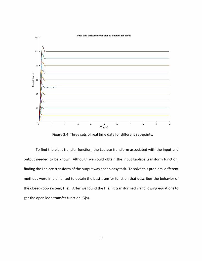
11

To find the plant transfer function, the Laplace transform associated with the input and

output needed to be known. Although we could obtain the input Laplace transform function,

finding the Laplace transform of the output was not an easy task. To solve this problem, different

methods were implemented to obtain the best transfer function that describes the behavior of

the closed-loop system, H(s). After we found the H(s), it transformed via following equations to

get the open loop transfer function, G(s).

Figure 2.4 Three sets of real time data for different set-points.

12

𝐻𝐻(𝑠𝑠) =𝐺𝐺(𝑠𝑠)

1 + 𝐺𝐺(𝑠𝑠)

𝐻𝐻(𝑠𝑠) ∗ �1 + 𝐺𝐺(𝑠𝑠)� = 𝐺𝐺(𝑠𝑠)

𝐻𝐻(𝑠𝑠) + 𝐻𝐻(𝑠𝑠)𝐺𝐺(𝑠𝑠) = 𝐺𝐺(𝑠𝑠)

𝐺𝐺(𝑠𝑠)�1 −𝐻𝐻(𝑠𝑠)� = 𝐻𝐻(𝑠𝑠)

𝐺𝐺(𝑠𝑠) =𝐻𝐻(𝑠𝑠)

1 − 𝐻𝐻(𝑠𝑠)

(4)

We can manipulate Equation (2) to obtain the analytical form of the G(s) (Equation (4)). Having

the closed loop transfer function, H(s), is a great advantage since it can be used to obtain the

plant transfer function, G(s), which was the main goal of our work.

Although the step after finding H(s) looks quite simple, finding H(s) was challenging. In

the next sections of this chapter, we discuss different tools that were used to solve this problem.

First the simplest form of the transfer function for the H(s), the second order transfer function,

is introduced to examine the general case. Then we added one zero to our pervious transfer

function and examined our new transfer function in detail. To complete our study a third order

transfer function was also studied in both cases, with and without one zero.

2.1 Second Order Transfer Function without Zero

To start, we assumed the simplest form of the transfer function for our system similar to

the one that is mentioned in Franklin’s published work [20]. In his work, he took advantage of

the pre-existing knowledge about the internal structure of his system that consisted of a motor.

13

It made the author start with the simple model of a motor with complex conjugate paired-poles

and no zeros. He used the basics of the control system to find the values for natural frequency

and damping ratio. In the time domain determining these parameters becomes a straightforward

task.

If we assume the motor’s transfer function in the frequency domain, it has the following form,

𝐺𝐺(𝑠𝑠) =𝑊𝑊𝑛𝑛

2

𝑠𝑠2 + 2𝜁𝜁𝑊𝑊𝑛𝑛𝑠𝑠 + 𝑊𝑊𝑛𝑛2

(5)

From acquired output data we were able to approximate the value for natural frequency and

damping ratio using the following equations.

𝑡𝑡𝑟𝑟𝑟𝑟𝑟𝑟𝑟𝑟 =1.8𝑤𝑤𝑛𝑛

(6)

𝑀𝑀𝑝𝑝% = 100 ∗ 𝑒𝑒−𝜉𝜉𝜉𝜉

�1−𝜉𝜉2�

(7)

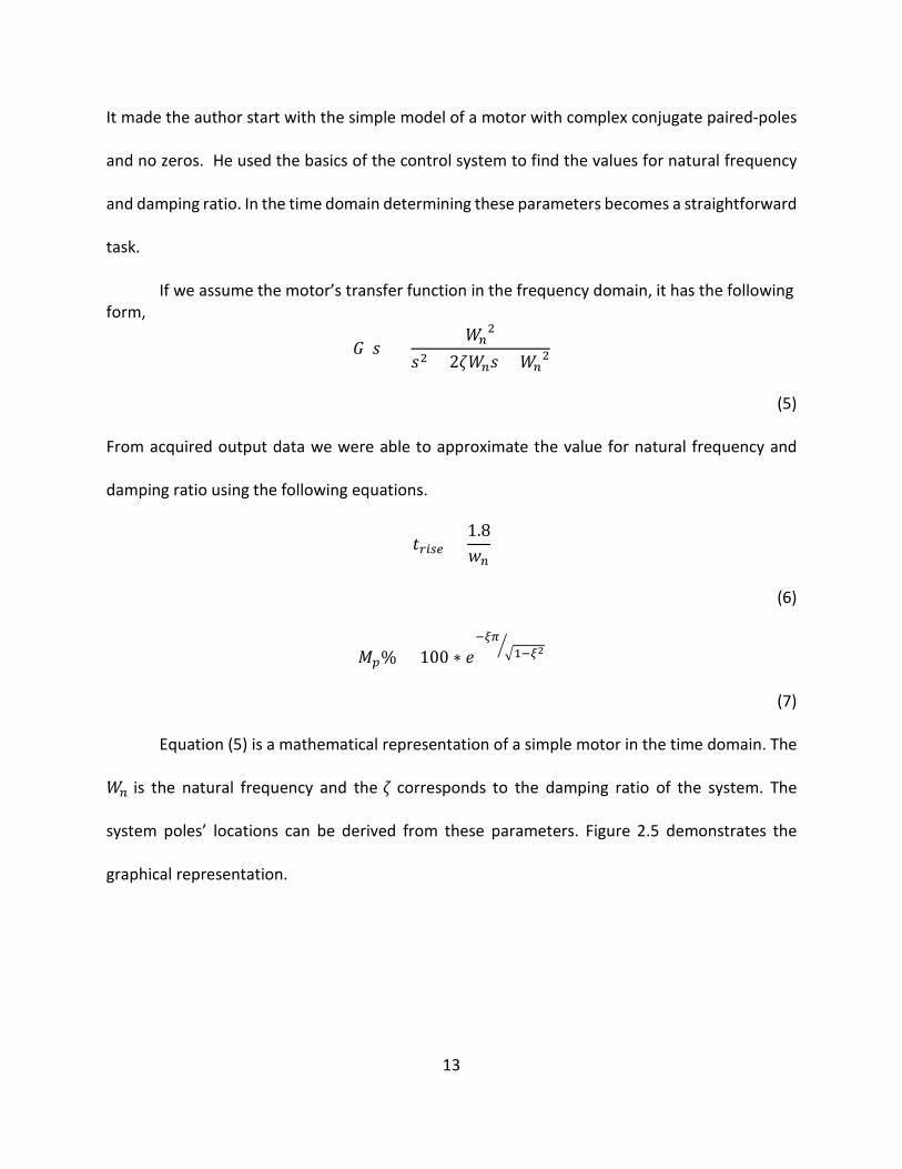
Equation (5) is a mathematical representation of a simple motor in the time domain. The

𝑊𝑊𝑛𝑛 is the natural frequency and the 𝜁𝜁 corresponds to the damping ratio of the system. The

system poles’ locations can be derived from these parameters. Figure 2.5 demonstrates the

graphical representation.

14

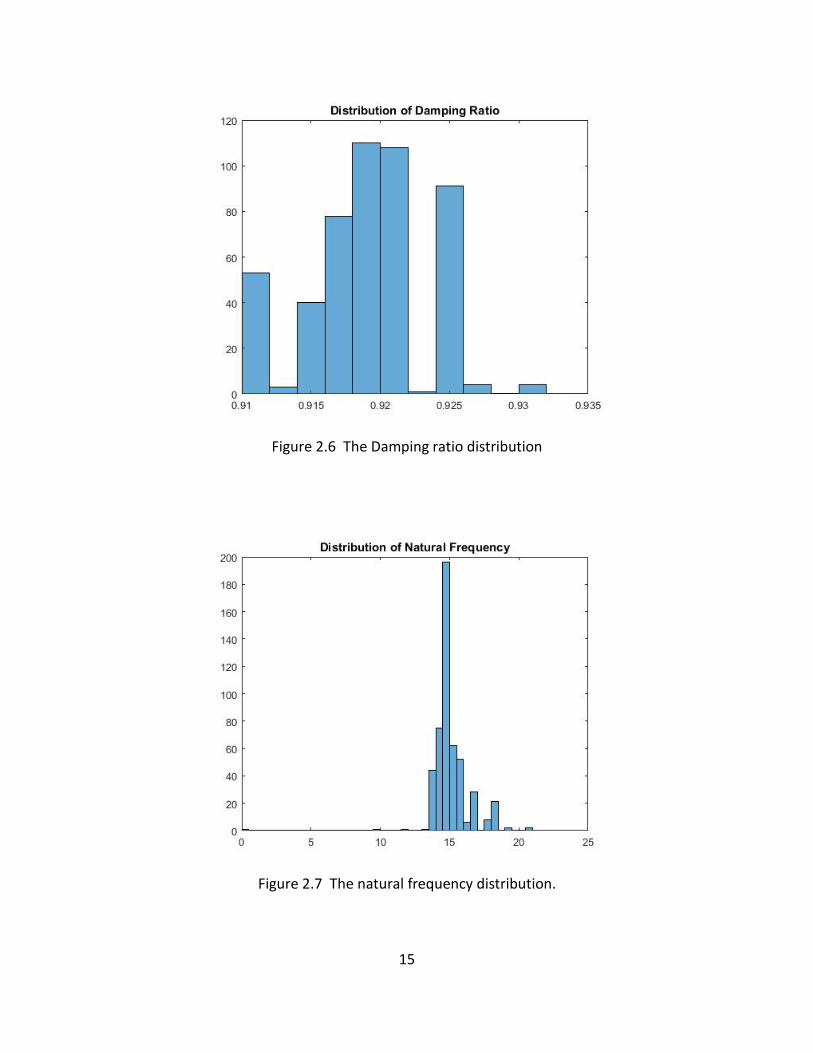
To estimate the poles' locations, we were required to use our 500 sets of acquired

experimental data. For each experiment, the natural frequency and the damping ratio had been

calculated with the help of Equations (5) and (6). These 500 sets of damping ratio and natural

frequency provided valuable information about the system. If all of the values for the natural

frequency and damping ratio were exactly the same, then the behavior of the system would be

similar to an ideal LTI system. Unfortunately, experimental results show differences among

derived values for the natural frequency and damping ratio. To understand the system, we

summarized both the natural frequency and the damping ratio into two separated histograms,

Figure 2.6 and Figure 2.7.

Figure 2.5 Damping ratio and natural frequency representation in the S

plain.

15

Figure 2.6 The Damping ratio distribution

Figure 2.7 The natural frequency distribution.

16

From Figure 2.6 and Figure 2.7 we can see both the natural frequencies and the damping ratios

are tightly grouped. Thus choosing the best value for both the natural frequency and the

damping ratio became a challenging problem. To address this problem, first a search algorithm

was used. Although search algorithms usually take a long time to operate, they can help to get

an idea about the system. In the algorithm, each set of the damping ratio and natural frequency

had been applied to the circuit shown in Figure 2.8 and the outputs of the system for different

set-point were sent to the workspace directly. Then for each experiment, the absolute

experimental value and the deviation between experimental and simulated value was stored in

a matrix form. Each row and column of our matrix represented damping ratios and natural

frequencies, correspondingly. After evaluating the deviation from the experimental data, the

best pair of the damping ratio and natural frequencies corresponds to a cell with the minimum

value that showed the least error.

Based on our search algorithm, the best pair of natural frequency and damping ratio had

the value of 𝑊𝑊𝑛𝑛 = 14.177 and 𝜁𝜁 = 0.922, correspondingly.

Figure 2.8 shows the schematic of the system, which was used for simulation. In this

simulation we considered the values we obtained from the search algorithm for the natural

frequency and the damping ratio.

Figure 2.8 Simulated circuit.

17

Figure 2.9 shows the simulation result in comparison with experimental data. Comparison

between the simulation results and the experimental data showed the same behavior and

characteristic while it suffered a significant mismatch.

Although the results of the simulation were not as we expected, they provided us with significant

amount of information. The ratio of experimental data over the simulated data was

approximately equal to 2. This meant that somewhere in the calculation a factor of 2 had been

missing. The promising approach to address this problem was to eliminate the steady state error.

Any system inside a close loops configuration can be thought as an open loop system with

a proportional controller in a feedback loop. Thus, the controller and the plant transfer function

could have the following form,

Figure 2.9 Steady state errors corresponding with the second order system chosen as transfer

function. The dashed line shows the simulation result and the solid line is the real data.

18

𝐶𝐶(𝑠𝑠) ∗ 𝐺𝐺(𝑠𝑠) = 𝐾𝐾𝑝𝑝 ∗𝑊𝑊𝑛𝑛

2


(8)

𝐾𝐾𝑝𝑝, the value indicating the gain for the controller, could be calculated from the steady state

value and the step value. Based on our collected data we obtained,

𝐾𝐾𝑝𝑝 = 1 .

(9)

So, the controller and plant transfer function could be written in the following format,

𝐶𝐶(𝑠𝑠) ∗ 𝐺𝐺(𝑠𝑠) = 1 ∗𝑊𝑊𝑛𝑛

2

𝑠𝑠2 + 2𝜁𝜁𝑊𝑊𝑛𝑛𝑠𝑠 + 𝑊𝑊𝑛𝑛2 .

(10)

The final value theorem confirmed our approximation for the steady state error of this transfer

function in a closed-loop format. Thus we can have,

𝐻𝐻𝑐𝑐𝑐𝑐(𝑠𝑠) =𝐺𝐺(𝑠𝑠)

1 + 𝐺𝐺(𝑠𝑠) ,

𝐻𝐻𝑐𝑐𝑐𝑐(𝑠𝑠) =

𝑊𝑊𝑛𝑛2


1 + 𝑊𝑊𝑛𝑛2


=𝑊𝑊𝑛𝑛

2

𝑠𝑠2 + 2𝜁𝜁𝑊𝑊𝑛𝑛𝑠𝑠 + 2𝑊𝑊𝑛𝑛2 ,

lim𝑟𝑟→0

𝑊𝑊𝑛𝑛2

𝑠𝑠2 + 2𝜁𝜁𝑊𝑊𝑛𝑛𝑠𝑠 + 2𝑊𝑊𝑛𝑛2 =

12

.

(11)

We started to approach this problem by assuming the following form for G(s),

19

𝐺𝐺(𝑠𝑠) = 𝐻𝐻𝑜𝑜𝑐𝑐(𝑠𝑠) =𝐾𝐾

𝑠𝑠2 + 𝑎𝑎𝑠𝑠 + 𝑏𝑏 .

(12)

Thus with the help of Equation (2), we could write the closed loop form of the same plant transfer

function,

𝐻𝐻𝑐𝑐𝑐𝑐(𝑠𝑠) =𝐾𝐾

𝑠𝑠2 + 𝑎𝑎𝑠𝑠 + 𝑏𝑏𝐾𝐾

𝑠𝑠2 + 𝑎𝑎𝑠𝑠 + 𝑏𝑏 + 1=

𝐾𝐾𝑠𝑠2 + 𝑎𝑎𝑠𝑠 + 𝑏𝑏 + 𝐾𝐾

=𝐾𝐾

𝑠𝑠2 + 𝑎𝑎𝑠𝑠 + 𝑏𝑏 + 𝐾𝐾 .

(13)

To eliminate the steady state error, we applied the final value theorem to the Equation (13) and

set the result of it to 1,

lim𝑟𝑟→0

𝐻𝐻𝑐𝑐𝑐𝑐(𝑠𝑠) = lim𝑟𝑟→0

𝐾𝐾𝑠𝑠2 + 𝑎𝑎𝑠𝑠 + 𝑏𝑏 + 𝐾𝐾

=𝐾𝐾

𝑏𝑏 + 𝐾𝐾= 1 ,

𝐾𝐾 = 𝑏𝑏 + 𝐾𝐾 .

(14)

Thus to have no steady state error, we obtained the following condition,

𝑏𝑏 = 0 .

(15)

With the new constrain on “𝑏𝑏” and Equation (13), we achieved,

𝐻𝐻𝑜𝑜𝑐𝑐(𝑠𝑠) =𝐾𝐾

𝑠𝑠2 + 𝑎𝑎𝑠𝑠=

𝐾𝐾𝑠𝑠(𝑠𝑠 + 𝑎𝑎)

.

(16)

These results mean the plant transfer function had to have a built-in integrator.

In this study, having outputs and inputs gave us the opportunity to approximate closed

loop transfer function directly. Thus, our focus for the rest of this section is on closed loop

20

systems. The open loop transfer function can be easily derived from closed loop system transfer

function by using Equation (4).

The transfer function for a closed loop system, considering Equation (16), could be

assumed,


𝑠𝑠2 + 𝑎𝑎𝑠𝑠 + 𝐾𝐾 .

(17)

Comparing the closed loop transfer function with the second order motor transfer

function led us to substitute the values in the closed loop transfer function with the damping

ratio and the natural frequency,


𝑠𝑠2 + 𝑎𝑎𝑠𝑠 + 𝐾𝐾≡

𝑊𝑊𝑛𝑛2

𝑠𝑠2 + 2𝜁𝜁𝑊𝑊𝑛𝑛𝑠𝑠 + 𝑊𝑊𝑛𝑛2 .

(18)

Thus, “𝐾𝐾” is substituted by the natural frequency squared while “𝑎𝑎” is substituted by two times

of the product of the natural frequency and the damping ratio in Equation (18); or,

𝐾𝐾 = 𝑊𝑊𝑛𝑛2 ,

𝑎𝑎 = 2𝜁𝜁𝑊𝑊𝑛𝑛 .

(19)

Considering these substitutions for the open loop transfer function, we wrote,

𝐻𝐻𝑜𝑜𝑐𝑐(𝑠𝑠) =𝐾𝐾

𝑠𝑠2 + 𝑎𝑎𝑠𝑠=

𝑊𝑊𝑛𝑛2

𝑠𝑠2 + 2𝜁𝜁𝑊𝑊𝑛𝑛𝑠𝑠 .

(20)

21

Finally, the inverse Laplace transform for the transfer function of a closed loop system had been

written,

ℒ−1�𝐻𝐻𝑐𝑐𝑐𝑐(𝑠𝑠)� = ℒ−1 �𝑊𝑊𝑛𝑛

2

𝑠𝑠2 + 2𝜁𝜁𝑊𝑊𝑛𝑛𝑠𝑠 + 𝑊𝑊𝑛𝑛2� =

𝑤𝑤 ∗ 𝑒𝑒(−𝑑𝑑𝑑𝑑𝑤𝑤𝑛𝑛) ∗ sin�𝑡𝑡𝑤𝑤𝑛𝑛�1 − 𝜁𝜁2�

�1 − 𝜁𝜁2 .

(21)

We obtained useful information about the plant transfer function from our collected data and a

simple math. The representation for the plant transfer function had to have a built-in integrator,

Equation (20), with the values we obtained from the search algorithm. The system model in

Figure 2.10 is based on this approximation. It is clear that the closed loop form of this plant is the

same as the plant we had studied before.

Our new model was tested. Figure 2.11 shows the experimented data in comparison with the

simulated data.

Figure 2.10 System model with an integrator.

22

To find the best fit, several Matlab tools were used, i.e. Matlab SystemIdentification tool. These

tools are mainly based on the least square estimation method that we had already used in our

search algorithm. We observed that using built-in Matlab tools was much faster than our in-

house search algorithm.

Matlab SystemIdentification tool estimated a slightly different closed-loop’s transfer

function than what was derived with our search algorithm. Equation (22) shows the closed-loop’s

transfer function suggested by the Matlab SystemIdentification tools.

Figure 2.11 Experimented data vs. simulated data.

23

𝐻𝐻𝑐𝑐𝑐𝑐(𝑠𝑠) =177.2

𝑠𝑠2 + 17.05𝑠𝑠 + 177.2

(22)

Using Equation (4), the open-loop’s transfer function can be rewritten in the following

form,

𝐺𝐺 =𝐻𝐻

1 − 𝐻𝐻=

177.2𝑠𝑠2 + 17.05𝑠𝑠 + 177.2

1 − 177.2𝑠𝑠2 + 17.05𝑠𝑠 + 177.2

=177.2

𝑠𝑠2 + 17.05𝑠𝑠=

177.2𝑠𝑠(𝑠𝑠 + 17.05)

.

(23)

The integrator in Equation (23) that was predicted is a part of the open loop system. The issue

that came to mind is how much this transfer function fits the data captured through different

experiments, generally speaking, how linear the system behaves in the linear region. To answer

this question, a very useful feature of Matlab SystemIdentification tool had been used. This

feature allows different time domain responses to be fed to the tool and to compute their

corresponding transfer function to see how they fit experiments.

For example, let us assume that the experimental data for the set point equal to 100 has

been fed to the Matlab SystemIdentification tool. The simulated results of that transfer function

were compared with the experimental data of set point equal to 10. The result is shown in Figure

2.12.

24

Matlab uses sophisticated algorithms like least square estimation method to evaluate

how precise the simulated data matches the experiment data. Matlab evaluated this transfer

function to be an 87.73 % match with the experimented data. Our objective was to make this

number as close to 100% as possible.

As the system worked in the linear region, the matching score had to be high. The

previous example is known as the worst-case scenario. The worst case scenario is when we try

to use the transfer function we derived by using the largest set-point, in our case 100 degrees,

and comparing the results from simulation using the same transfer function for our smallest set-

point, in our case 10 degrees. As 10 and 100 degrees are located in the borders of the linear

region, thus we observed the maximum difference between simulated results and experimental

data.

To prove this hypothesis, 10 different set points had been fed to the SystemIdentification

tool and their corresponding transfer functions were tested with different experimented data to

see how closely they matched. The matching scores are listed in Table 2-1.

Figure 2.12 (Data 1): transfer function derived from set point equal to 100, (Data 2):

experimental data for set-point equal to 10.

25


with the different experiment.

S.P Transfer function 100 90 80 70 60 50 40 30 20 10 Average

10

0

177.2𝑠𝑠2 + 17.05𝑠𝑠 + 177.2 95.17 96.29 95.74 95.16 93.81 93.66 93.4 91.71 89.1 87.73 93.177

90 186.5𝑠𝑠2 + 17.84𝑠𝑠 + 186.5

95.06 96.43 96.08 95.65 94.46 94.22 93.94 92.3 89.72 88.46 93.632

80 193.8𝑠𝑠2 + 18.56𝑠𝑠 + 193.8 94.79 96.32 96.19 95.98 94.91 94.52 94.21 92.64 90.12 89.01 93.869

70 199𝑠𝑠2 + 19.33𝑠𝑠 + 199 94.35 95.92 96.03 96.14 95.11 94.45 94.12 92.64 90.26 89.37 93.839

60 222.7𝑠𝑠2 + 20.71𝑠𝑠 + 222.7 93.55 95.2 95.5 95.65 95.49 94.94 94.65 93.43 91.03 90.3 93.974

50 222.8𝑠𝑠2 + 20.15𝑠𝑠 + 222.9 93.6 95.17 95.35 95.21 95.29 95.12 94.89 93.68 91.18 90.22 93.971

40 225.4𝑠𝑠2 + 20.21𝑠𝑠 + 225.4

93.44 94.98 95.16 94.99 95.2 95.11 94.91 93.75 90.26 90.28 93.808

30 244𝑠𝑠2 + 21.24𝑠𝑠 + 244 92.31 93.76 94.08 94 94.8 94.81 94.7 93.92 91.67 90.89 93.494

20 279.2𝑠𝑠2 + 23.2𝑠𝑠 + 279.3 90.02 91.33 91.8 91.84 93.34 93.44 93.49 93.39 91.97 91.68 92.23

10 327.4𝑠𝑠2 + 26.65𝑠𝑠 + 327.5 87.66 88.93 89.55 89.81 91.62 91.49 91.63 91.9 91.54 92.12 90.625

In Table 2-1, each row represents one transfer function. The transfer function in each row was

derived from the experiment data whose set-point is represented in the first column. Third to

12th columns represent the matching score between simulation data and the experimented data

with the set-point represented in the first row.

26

Notice the green cell in the table. The transfer function derived from the experiment with

set-point equal to 80 degrees had been simulated. The value of 80 degrees comes from the first

column, fourth row. The result was compared with the experiment with set-point equal to 50

degrees. The value of 50 degrees comes from the first row, 8th column. The green cell shows that

the simulated data matches the real experiment about 94.5% with a different set-point.

The last column of the table shows the average of all matching percentage in a row which

can be used to find the best fit for all the experiments. This value also can be used to compare

different transfer functions.

To study the case even more precisely, the open-loop’s transfer function associated with

each of the closed-loop’s transfer function and the open-loop’s poles had been derived in the

Table 2-2.

27

Table 2-2 Poles in open loop and closed loop form.

S.P Transfer function CL pole OL TF OL pole

100 177.2

𝑠𝑠2 + 17.05𝑠𝑠 + 177.2

-8.5250

±10.2237i

177.2𝑠𝑠2 + 17.05𝑠𝑠

-17.05

90 186.5

𝑠𝑠2 + 17.84𝑠𝑠 + 186.5

-8.9200

±10.3409i

186.5𝑠𝑠2 + 17.84𝑠𝑠

-17.84

80 193.8

𝑠𝑠2 + 18.56𝑠𝑠 + 193.8

-9.2800

±10.3770i

193.8𝑠𝑠2 + 18.56𝑠𝑠

-18.56

70 199

𝑠𝑠2 + 19.33𝑠𝑠 + 199

-9.6650

±10.2756i

199𝑠𝑠2 + 19.33𝑠𝑠

-19.33

60 222.7

𝑠𝑠2 + 20.71𝑠𝑠 + 222.7

-10.3550

±10.7459i

222.7𝑠𝑠2 + 20.71𝑠𝑠

-20.71

50 222.8

𝑠𝑠2 + 20.15𝑠𝑠 + 222.9

-10.0750

±11.0179i

222.8𝑠𝑠2 + 20.15𝑠𝑠

-20.15

40 225.4

𝑠𝑠2 + 20.21𝑠𝑠 + 225.4

-10.1050

±11.1036i

225.4𝑠𝑠2 + 20.21𝑠𝑠

-20.21

30 244

𝑠𝑠2 + 21.24𝑠𝑠 + 244

-10.6200

±11.4549i

244𝑠𝑠2 + 21.24𝑠𝑠

-21.24

20 279.2

𝑠𝑠2 + 23.2𝑠𝑠 + 279.3

-11.6000

±12.0308i

279.2𝑠𝑠2 + 23.2𝑠𝑠

-23.2

10 327.4

𝑠𝑠2 + 26.65𝑠𝑠 + 327.5

-13.3250

±12.2452i

327.4𝑠𝑠2 + 26.65𝑠𝑠

-26.65

Pole location is generally responsible for system behavior. As shown in Table 2-2, the closed-

loop’s poles locations are approximately in the same place. By increasing the set–point, both real

28

part and imaginary part of the poles decreased. The imaginary part is responsible for the duration

of the over-shoot, and the real part indicates how long it takes for the over-shoot to be damped.

By taking a look over Figure 2.4, it is clear that by increasing the set-point, the duration of the

over-shoot increased also. This means that the closer the set-point comes to equaling 100, the

less the over-shoot is damped.

As shown in Table 2-2, the open loop pole location changes slightly for different transfer

function. Thus the gain decreased as the set point increased. These changes are because of the

difference between time domain’s characteristics of the system in response to the different set-

points.

To have a better understanding, take a look over Figure 2.13, which represents system

time domain’s representation distribution versus set-point.

29

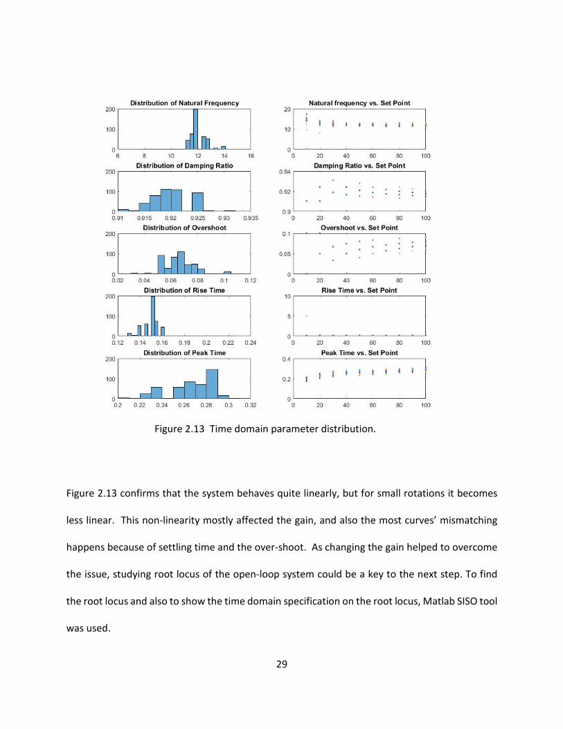
Figure 2.13 confirms that the system behaves quite linearly, but for small rotations it becomes

less linear. This non-linearity mostly affected the gain, and also the most curves’ mismatching

happens because of settling time and the over-shoot. As changing the gain helped to overcome

the issue, studying root locus of the open-loop system could be a key to the next step. To find

the root locus and also to show the time domain specification on the root locus, Matlab SISO tool

was used.

Figure 2.13 Figure 2.13 Time domain parameter distribution.

30

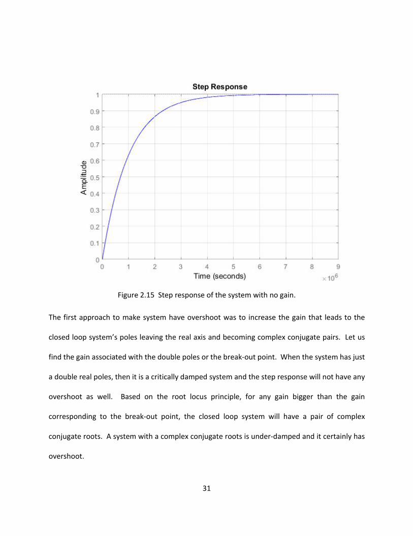
The step response of the system with no gain is shown in Figure 2.15, which as can be

seen does not have any overshoot. In the root locus, Figure 2.14, the pink points show the closed-

loop system’s poles associated with the assigned gain. As long as the poles lie on the real axis

there will be no over shoot, and the system is placed in the over damped group.

Figure 2.14 System root locus with no gain.

31

The first approach to make system have overshoot was to increase the gain that leads to the

closed loop system’s poles leaving the real axis and becoming complex conjugate pairs. Let us

find the gain associated with the double poles or the break-out point. When the system has just

a double real poles, then it is a critically damped system and the step response will not have any

overshoot as well. Based on the root locus principle, for any gain bigger than the gain

corresponding to the break-out point, the closed loop system will have a pair of complex

conjugate roots. A system with a complex conjugate roots is under-damped and it certainly has

overshoot.

Figure 2.15 Step response of the system with no gain.

32

To find the gain associated with the break-out point, the following calculations were

essential.

𝐺𝐺(𝑠𝑠) =𝐾𝐾

𝑠𝑠(𝑠𝑠 + 17)

𝐾𝐾 = 𝜎𝜎(𝜎𝜎 + 17)

𝑑𝑑𝐾𝐾𝑑𝑑𝜎𝜎

= 2𝜎𝜎 + 17

𝑑𝑑𝐾𝐾𝑑𝑑𝜎𝜎

= 0

2𝜎𝜎 + 17 = 0

𝜎𝜎 = −8.5

𝐻𝐻(𝑠𝑠) = 𝐾𝐾

𝑠𝑠(𝑠𝑠 + 17) + 𝐾𝐾

𝑖𝑖𝑖𝑖 𝑠𝑠 = −8.5 → 𝑠𝑠(𝑠𝑠 + 17) + 𝐾𝐾 = 0 𝐾𝐾 = 72.25

(23)

Based on the result, derived from Equation (23), for any gain bigger than 72.25, the system would

experience over-shoot. Also, the minimum settling time in an under-damped situation happened

in gains close to this gain. If K=72.25 applied to the system, the minimum settling time would be

observed. The reason was the real part of the closed loop’s poles, 𝜎𝜎, is maximum in the break-

out point in this case.

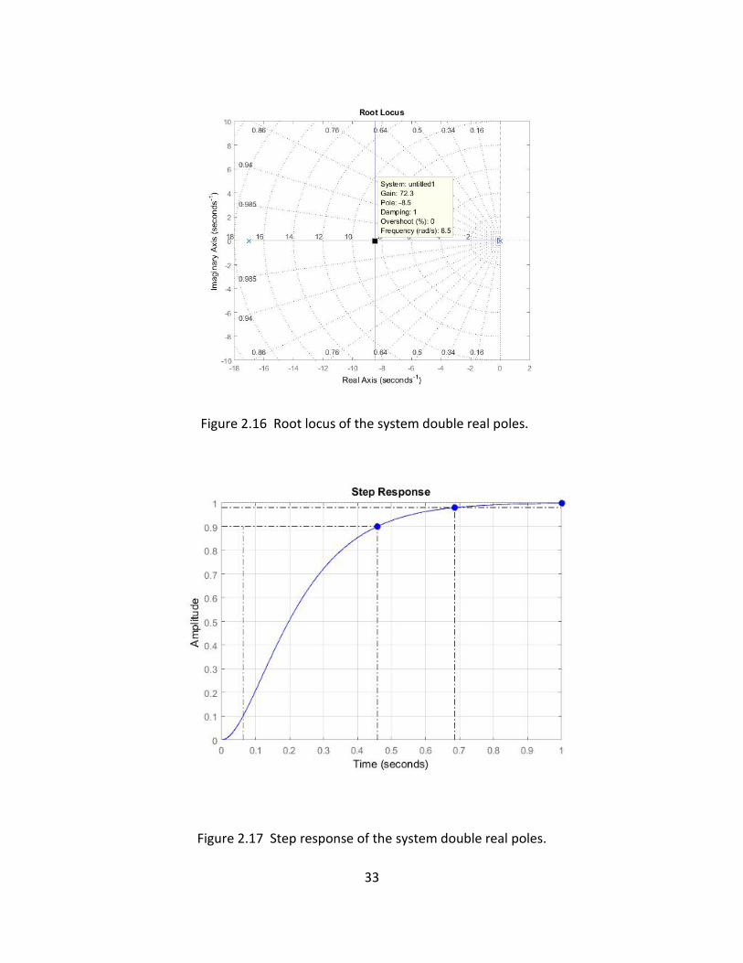
The following root locus (Figure 2.16) and associated step function response (Figure 2.17)

confirmed the results that had been achieved through calculation.

33

Figure 2.17 Step response of the system double real poles.

Figure 2.16 Root locus of the system double real poles.

34

Increasing the gain would result in overshoot. To see which gain worked the best, time domain

requirement had to be considered. The parameter that caused the most discrepancy between

the simulated and experimented data was the settling time. Based on the experimented data,

the settling time had to be less than 0.4 second, so that,

𝑇𝑇𝑟𝑟 = −4.6𝜎𝜎

𝜎𝜎 = −4.6𝑇𝑇𝑟𝑟

(24)

By plugging the experimental data into Equation (24), the following value for 𝜎𝜎 was achieved.

𝜎𝜎 = −4.60.4

= −11.5

(25)

On the other hand, the maximum settling time happened for the gain in the break-out point. To

obtain that gain, the following calculations were essential.

𝐺𝐺(𝑠𝑠) =𝑘𝑘

𝑠𝑠(𝑠𝑠 + 17)

𝑘𝑘 = 𝜎𝜎(𝜎𝜎 + 17)

𝑑𝑑𝑘𝑘𝑑𝑑𝜎𝜎

= 2𝜎𝜎 + 17


= 0

2𝜎𝜎 + 17 = 0

𝜎𝜎 = −8.5

(26)

35

This meant that with the current transfer function, the desired settling time could not be

achieved. To confirm this calculation, the root locus of the transfer function has been provided

in Figure 2.18.

Figure 2.18 shows the system root locus, by using Matlab SISO tool. SISO tool provides

the user with a very useful option. Using this option, the user can indicate the required time

domain characteristics. Matlab SISO tool, based on the time domain demands, indicates the area

on the S plan while keeping the system in the closed loop poles’ locations condition. For example,

in Figure 2.18, if the closed loop poles were located in the yellow area, then the desired settling

time could not be met.

As can be seen in Figure 2.18, the roots that are located in the yellow region cannot meet

the expectation. To address this problem, the pole location needed to be changed.

𝜎𝜎 = −12

Figure 2.18 System root locus with time domain requirement specified region.

36

𝐺𝐺(𝑠𝑠) =𝑘𝑘

𝑠𝑠(𝑠𝑠 + 𝑝𝑝)

𝑘𝑘 = 𝜎𝜎(𝜎𝜎 + 𝑝𝑝)


= 2𝜎𝜎 + 𝑝𝑝


= 0

2𝜎𝜎 + 𝑝𝑝 = 0

2(12) + 𝑝𝑝 = 0

𝑝𝑝 = −24

(27)

To confirm the calculation, consider Figure 2.19 and Figure 2.20, representing the system root

locus and the system step response after applying changes.

Figure 2.19 System root locus with time domain requirement

satisfied.

37

Although this issue had been addressed, finding the best match which fits all the set-points

requires more calculations.

Having the system transfer function in second order allowed us to find the time domain

representation of the system’s step response.

𝐻𝐻𝑜𝑜𝑐𝑐(𝑠𝑠) =𝑊𝑊𝑛𝑛

2

𝑠𝑠2 + 2𝜁𝜁𝑊𝑊𝑛𝑛𝑠𝑠

𝐻𝐻𝑐𝑐𝑐𝑐(𝑠𝑠) =𝑊𝑊𝑛𝑛

2


ℒ−1�𝐻𝐻𝑐𝑐𝑐𝑐(𝑠𝑠)� = ℒ−1 �1𝑠𝑠∗

𝑊𝑊𝑛𝑛2

𝑠𝑠2 + 2𝜁𝜁𝑊𝑊𝑛𝑛𝑠𝑠 + 𝑊𝑊𝑛𝑛2� =

Figure 2.20 System step response with time domain requirement

satisfied.

38

𝑦𝑦(𝑡𝑡) = 1 − 𝑒𝑒−𝜁𝜁𝑊𝑊𝑛𝑛𝑑𝑑 ∗ �cos �𝑊𝑊𝑛𝑛�1 − 𝜁𝜁2 ∗ 𝑡𝑡� +𝜁𝜁

�1 − 𝜁𝜁2∗ sin �𝑊𝑊𝑛𝑛�1 − 𝜁𝜁2 ∗ 𝑡𝑡��

(28)

So to find the best values matching all values of set points, the normalized averaged curve was

used. This curve is made by 500 different experiments, which were normalized. The result is the

curve shown in Figure 2.21.

Figure 2.21 System step response with time domain requirement satisfied.

39

To compare the simulated result and the normalized average result, only the first 0.45 seconds

is depicted in Figure 2.21. The most discrepancy happened in this small region, and after 0.45

seconds both simulation and experiments fit to each other perfectly.

As is shown in Figure 2.22, although the settling time issue had been addressed, the rise

time is not the same. To solve this issue, a closer look at the rise time, which relates to natural

frequency and damping ratio, was needed.

Using the Matlab SystemIdentification tool for the averaged normalized data suggested

the following transfer function.

Figure 2.22 Normalized averaged experiment vs simulation result.

40

The transfer function presented by Equation (28) and the open loop corresponding transfer

function has been derived in Equation (29).

𝐻𝐻𝑐𝑐𝑐𝑐 =218.6

𝑠𝑠2 + 20.39𝑠𝑠 + 218.6

(28)

𝐻𝐻0𝑐𝑐 =218.6

𝑠𝑠(𝑠𝑠 + 20.39)

(29)

Figure 2.24 Simulation data and averaged normalized data.

Figure 2.23 Root locus.

41

As shown in Figure 2.24 and Figure 2.23, the simulated data perfectly fit the averaged normalized

data. The issue was how well this transfer function fit the sets of set-points. The same feature

that had been used previously to evaluate the matching score was used again to find the

matching score between the transfer function derived from the averaged normalized data and

the experimental data associated with each of the set-points. The percent matching score is

summarized in Table 2-3.

Table 2-3 Matching rate of the final transfer functions with 2 poles and no zero comparing with the different experiment

As each of these 500 sets of experiments have different time requirements, there is no unique

transfer function that fits all of them, so instead of each curve itself, the averaged normalized

curve had been used. The average of matching for the transfer function derived from averaged

normalized data was slightly better than the best averaged derived in Table 2-1. It showed that

using the averaged normalized data helped to get a better result.

In the next section, adding a zero and its contribution will be tested.


100 218.6

𝑠𝑠2 + 20.39𝑠𝑠 + 218.6 93.76 95.41 95.67 95.77 95.48 94.95 94.66 93.38 90.94 90.15 94.017

42

2.2 Second Order Transfer Function with One Zero

The highest rate of matching score using a second order transfer function with no zero

was about 94%. One method of increasing this value is to add a zero and study system behavior.

To make a better fit, instead of the usual second order transfer function, the general form

of the transfer function was studied. The equation for the general form of second order transfer

function with one zero first needed to satisfy certain requirements. It had the following form

(Equation (30)).

𝐻𝐻𝑜𝑜𝑐𝑐(𝑠𝑠) =𝐾𝐾(𝑠𝑠 + 𝑧𝑧)𝑠𝑠2 + 𝑎𝑎𝑠𝑠 + 𝑏𝑏

(30)

As had been discussed before, by having output and input data of the experiment, the

closed loop system transfer function could be studied directly. After finding the best fit for the

closed loop transfer function, the open loop transfer function could be derived. In this step, the

closed loop transfer function associated with Equation (30) had to be calculated.

Equation (31) shows the calculation to achieve the closed loop transfer function.

𝐻𝐻𝑐𝑐𝑐𝑐(𝑠𝑠) =𝐾𝐾(𝑠𝑠 + 𝑧𝑧)𝑠𝑠2 + 𝑎𝑎𝑠𝑠 + 𝑏𝑏𝐾𝐾(𝑠𝑠 + 𝑧𝑧)𝑠𝑠2 + 𝑎𝑎𝑠𝑠 + 𝑏𝑏 + 1

=𝐾𝐾(𝑠𝑠 + 𝑧𝑧)

𝑠𝑠2 + 𝑎𝑎𝑠𝑠 + 𝑏𝑏 + 𝐾𝐾(𝑠𝑠 + 𝑧𝑧) =𝐾𝐾(𝑠𝑠 + 𝑧𝑧)

𝑠𝑠2 + (𝑎𝑎 + 𝐾𝐾)𝑠𝑠 + 𝑏𝑏 + 𝐾𝐾𝑧𝑧

(31)

Having the closed loop transfer function from Equation (31) and using final theorem principle,

one can estimate the valid region for the coefficients in the closed loop form.

43

lim𝑟𝑟→0

𝐻𝐻𝑐𝑐𝑐𝑐(𝑠𝑠) = lim𝑟𝑟→0

𝐾𝐾(𝑠𝑠 + 𝑧𝑧)𝑠𝑠2 + (𝑎𝑎 + 𝐾𝐾)𝑠𝑠 + 𝑏𝑏 + 𝐾𝐾𝑧𝑧

=𝐾𝐾𝑧𝑧

𝐾𝐾𝑧𝑧 + 𝑏𝑏= 1

𝐾𝐾𝑧𝑧 = 𝐾𝐾𝑧𝑧 + 𝑏𝑏

(32)

To have the steady state equal to zero, the following condition had to be met:

𝑏𝑏 = 0

(33)

If the value for “𝑏𝑏” is plugged into Equation (30), which showed the open loop transfer function,

then we have Equation (34).

𝐻𝐻𝑜𝑜𝑐𝑐(𝑠𝑠) =𝐾𝐾(𝑠𝑠 + 𝑧𝑧)𝑠𝑠2 + 𝑎𝑎𝑠𝑠

(34)

Besides the steady state error, which was taken care of in the previous steps, the system stability

was also crucial. For the open loop system to be stable, the following condition had to be met.

𝑎𝑎 > 0

(35)

As long as the value for “𝑎𝑎” is a positive value, the pole remained in LHP, which guaranteed the

system stability.

Using feedback usually improves the system, but sometimes the feedback loop itself

makes the system unstable. Besides, for stability in the closed loop transfer function, having

complex conjugate poles is essential to make the system have overshoots. So, by the following

calculation the region that makes this happen was specified.

𝐻𝐻𝑐𝑐𝑐𝑐(𝑠𝑠) =𝐾𝐾(𝑠𝑠 + 𝑧𝑧)

𝑠𝑠2 + (𝑎𝑎 + 𝐾𝐾)𝑠𝑠 + 𝐾𝐾𝑧𝑧

44

(𝑎𝑎 + 𝐾𝐾) > 0

(𝑎𝑎 + 𝐾𝐾)2 − 4𝐾𝐾𝑧𝑧 < 0

(36)

If the condition provided in the Equation (36) is satisfied, then the closed loop system willhave a

pair of complex conjugate poles, as in Equation (37).

𝑠𝑠1,2 =−(𝑎𝑎 + 𝐾𝐾) + �(𝑎𝑎 + 𝐾𝐾)2 − 4𝐾𝐾𝑧𝑧

2

(37)

If these values are substituted in the equation, by using partial fraction method, the transfer

function can be simplified (Equation (38)).


𝑠𝑠2 + (𝑎𝑎 + 𝐾𝐾)𝑠𝑠 + 𝐾𝐾𝑧𝑧=

𝐴𝐴𝑠𝑠 + 𝑝𝑝

+𝐵𝐵

𝑠𝑠 + �̅�𝑝

𝐴𝐴 =−𝑘𝑘2

+ 𝑗𝑗𝑘𝑘 �−(𝑎𝑎 + 𝐾𝐾)

2 + 𝑧𝑧�

2�4𝐾𝐾𝑧𝑧−(𝑎𝑎 + 𝐾𝐾)22

𝐵𝐵 =−𝑘𝑘2− 𝑗𝑗

𝑘𝑘(−(𝑎𝑎 + 𝐾𝐾)2 + 𝑧𝑧)


𝑝𝑝 =−(𝑎𝑎 + 𝐾𝐾)

2+ 𝑗𝑗

�4𝐾𝐾𝑧𝑧−(𝑎𝑎 + 𝐾𝐾)2

2

(38)

By applying these values in the simplified form for the transfer function, we could find the Laplace

inverse of the closed loop system directly.

45


𝑠𝑠2 + (𝑎𝑎 + 𝐾𝐾)𝑠𝑠 + 𝐾𝐾𝑧𝑧

=

2 �−𝑘𝑘2 �𝑠𝑠 + (𝑎𝑎 + 𝐾𝐾)2 � +

𝑘𝑘 �−(𝑎𝑎 + 𝐾𝐾)2 + 𝑧𝑧�


��4𝐾𝐾𝑧𝑧−(𝑎𝑎 + 𝐾𝐾)22 ��

�𝑠𝑠 + (𝑎𝑎 + 𝐾𝐾)2 �

2+ ��4𝐾𝐾𝑧𝑧−(𝑎𝑎 + 𝐾𝐾)2

2 �2

ℒ−1�𝐻𝐻𝑐𝑐𝑐𝑐(𝑠𝑠)� = −𝑘𝑘 ∗ 𝑒𝑒−(𝑎𝑎+𝐾𝐾)2 𝑑𝑑 �cos�

�4𝐾𝐾𝑧𝑧−(𝑎𝑎 + 𝐾𝐾)2

2𝑡𝑡� −

(𝑎𝑎 + 𝑧𝑧)𝑏𝑏

sin��4𝐾𝐾𝑧𝑧−(𝑎𝑎 + 𝐾𝐾)2

2𝑡𝑡��

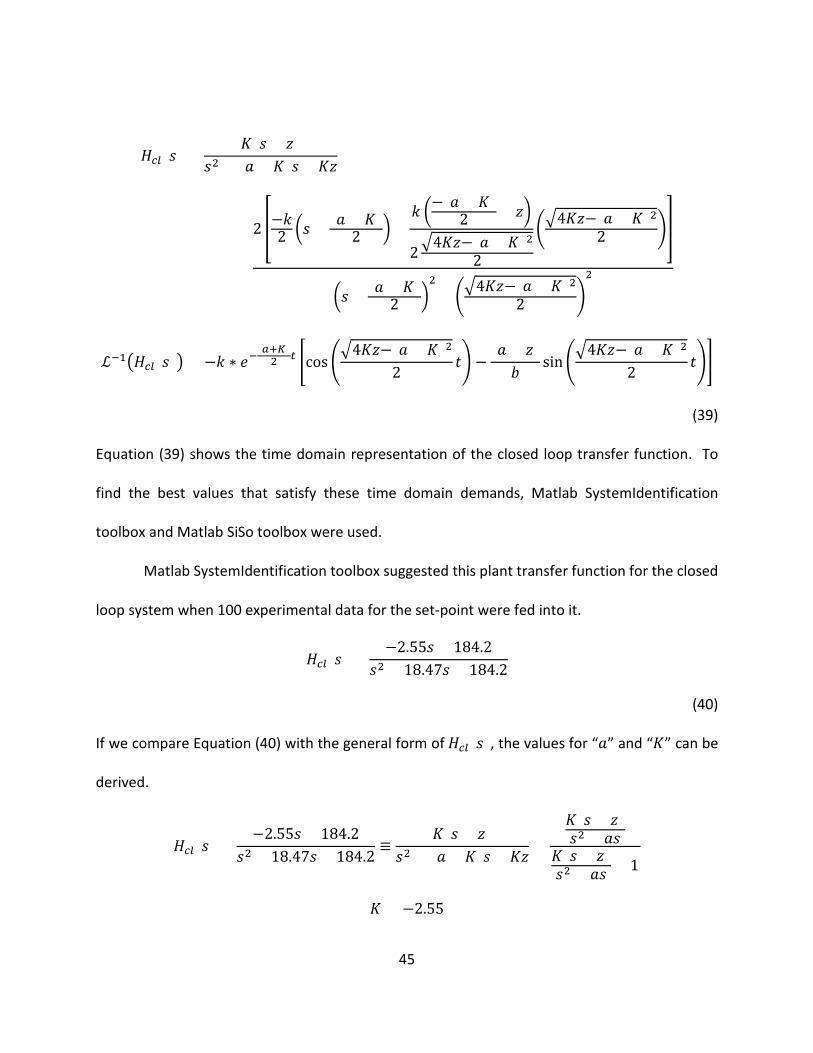
(39)

Equation (39) shows the time domain representation of the closed loop transfer function. To

find the best values that satisfy these time domain demands, Matlab SystemIdentification

toolbox and Matlab SiSo toolbox were used.

Matlab SystemIdentification toolbox suggested this plant transfer function for the closed

loop system when 100 experimental data for the set-point were fed into it.

𝐻𝐻𝑐𝑐𝑐𝑐(𝑠𝑠) =−2.55𝑠𝑠 + 184.2

𝑠𝑠2 + 18.47𝑠𝑠 + 184.2

(40)

If we compare Equation (40) with the general form of 𝐻𝐻𝑐𝑐𝑐𝑐(𝑠𝑠), the values for “𝑎𝑎” and “𝐾𝐾” can be

derived.

𝐻𝐻𝑐𝑐𝑐𝑐(𝑠𝑠) =−2.55𝑠𝑠 + 184.2

𝑠𝑠2 + 18.47𝑠𝑠 + 184.2≡

𝐾𝐾(𝑠𝑠 + 𝑧𝑧)𝑠𝑠2 + (𝑎𝑎 + 𝐾𝐾)𝑠𝑠 + 𝐾𝐾𝑧𝑧

=𝐾𝐾(𝑠𝑠 + 𝑧𝑧)𝑠𝑠2 + 𝑎𝑎𝑠𝑠

𝐾𝐾(𝑠𝑠 + 𝑧𝑧)𝑠𝑠2 + 𝑎𝑎𝑠𝑠 + 1

𝐾𝐾 = −2.55

46

𝑧𝑧 = −184.22.55

= −72.23

𝑎𝑎 = 18.47 − (−2.55) = 21.022

(41)

Equation (41) confirmed the condition provided at the beginning of this section for “𝑎𝑎” and “𝐾𝐾”.

The next step was to find the time domain representation of the closed loop transfer

function using inverse Laplace transfer function (Equation (42)).

2 �−𝑘𝑘2 �𝑠𝑠 + (𝑎𝑎 + 𝐾𝐾)2 � + 𝑘𝑘(𝑎𝑎 + 𝑧𝑧)

2𝑏𝑏 ��4𝐾𝐾𝑧𝑧−(𝑎𝑎 + 𝐾𝐾)22 ��

�𝑠𝑠 + (𝑎𝑎 + 𝐾𝐾)2 �

2+ ��4𝐾𝐾𝑧𝑧−(𝑎𝑎 + 𝐾𝐾)2

2 �2 =

−2.55[(𝑠𝑠 + 9.24) + (10.445 ∗ 9.95)](𝑠𝑠 + 9.24)2 + (9.95)2

ℒ−1�𝐻𝐻𝑐𝑐𝑐𝑐(𝑠𝑠)� = −2.55 ∗ 𝑒𝑒−9.24𝑑𝑑[cos(9.95𝑡𝑡) + 10.445 sin(9.95𝑡𝑡)]

(42)

Also by having the values for “a”, “K”, and “z” and plugging them into Equation (34), the open

loop system transfer function could be derived (Equation (43)).

𝐻𝐻𝑜𝑜𝑐𝑐(𝑠𝑠) =𝐾𝐾(𝑠𝑠 + 𝑧𝑧)𝑠𝑠2 + 𝑎𝑎𝑠𝑠

=−2.55(𝑠𝑠 − 72.23)𝑠𝑠(𝑠𝑠 + 21.022)

(43)

To study the case more carefully, the root locus representation of the system with following

system demand is drawn in Figure 2.25. The time domain demands, derived from the

experimented data for set-point, equals 100.

47

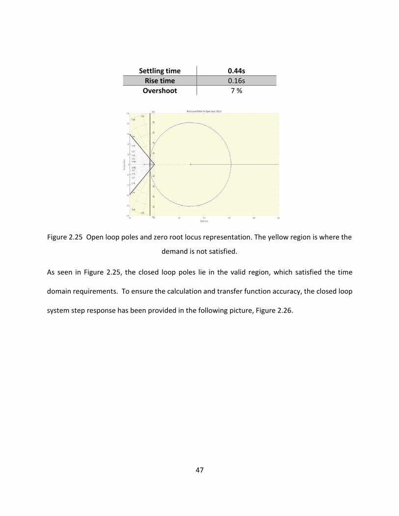
Settling time 0.44s Rise time 0.16s

Overshoot 7 %

As seen in Figure 2.25, the closed loop poles lie in the valid region, which satisfied the time

domain requirements. To ensure the calculation and transfer function accuracy, the closed loop

system step response has been provided in the following picture, Figure 2.26.

Figure 2.25 Open loop poles and zero root locus representation. The yellow region is where the

demand is not satisfied.

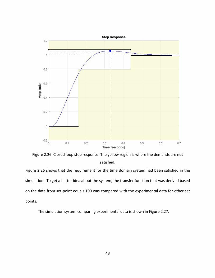
48

Figure 2.26 shows that the requirement for the time domain system had been satisfied in the

simulation. To get a better idea about the system, the transfer function that was derived based

on the data from set-point equals 100 was compared with the experimental data for other set

points.

The simulation system comparing experimental data is shown in Figure 2.27.

Figure 2.26 Closed loop step response. The yellow region is where the demands are not

satisfied.

49

As the system is not perfectly linear, so the transfer function at different set point had been

extracted and the comparison results have been presented in the following table, Table 2-4.

Figure 2.27 Closed loop step response. Dashed line show the simulation result and the solid line is the

experimental data.

50

Table 2-4 Matching score of the different transfer functions with 2 poles and one zero

comparing the different experiments.


100 −1.256𝑠𝑠 + 177.1𝑠𝑠2 + 17.05𝑠𝑠 + 177.1

95.17 96.29 95.73 95.16 93.81 93.66 93.4 91.71 89.1 87.72 93.175

90 −2.095𝑠𝑠 + 186.5𝑠𝑠2 + 17.83𝑠𝑠 + 186.5

95.06 96.43 96.08 95.65 94.46 94.22 93.94 92.3 89.72 88.46 93.632

80 −1.928𝑠𝑠 + 193.8

𝑠𝑠2 + 18.56𝑠𝑠 + 193.8 94.79 96.32 96.19 95.98 94.91 94.52 94.21 92.64 90.12 89.01 93.869

70 −2.044𝑠𝑠 + 199

𝑠𝑠2 + 19.33𝑠𝑠 + 199.1 94.35 95.92 96.03 96.14 95.11 94.45 94.12 92.65 90.26 89.37 93.84

60 −2.144𝑠𝑠 + 222.7

𝑠𝑠2 + 20.71𝑠𝑠 + 222.8 93.55 95.2 95.5 95.65 95.49 94.94 94.65 93.43 91.03 90.3 93.974

50 −2.409𝑠𝑠 + 222.8

𝑠𝑠2 + 20.14𝑠𝑠 + 222.9 93.61 95.17 95.35 95.21 95.29 95.12 94.89 93.68 91.18 90.22 93.972

40 −2.446𝑠𝑠 + 225.4

𝑠𝑠2 + 20.21𝑠𝑠 + 225.5 93.44 94.98 95.16 94.99 95.2 95.11 94.91 93.75 91.26 90.28 93.908

30 −3.112𝑠𝑠 + 243.9𝑠𝑠2 + 21.25𝑠𝑠 + 244

92.30 93.76 94.08 94 94.8 94.81 94.7 93.92 91.67 90.89 93.493

20 −1.995𝑠𝑠 + 279.2𝑠𝑠2 + 23.2𝑠𝑠 + 279.2

90.02 91.33 91.8 91.84 93.34 93.44 93.49 93.39 91.97 91.68 92.23

10 −3.584𝑠𝑠 + 327.4

𝑠𝑠2 + 26.65𝑠𝑠 + 327.5 87.66 88.93 89.55 89.81 91.62 91.49 91.63 91.9 91.54 92.12 90.625

Comparing Table 2-1and Table 2-4 showed that adding the zero does not improve the estimated

system transfer function. To study this case, the open loop transfer functions had been derived

in Table 2-5 . The values for open loop zero and poles had also been added to the table.

51

Table 2-5 Poles in open loop and closed loop form.

S.P Transfer function OL TF OL pole OL zero

100 −1.256𝑠𝑠 + 177.1

𝑠𝑠2 + 17.05𝑠𝑠 + 177.1 −1.256𝑠𝑠 + 177.1

𝑠𝑠2 + 18.3𝑠𝑠 -18.3 -141.0

90 −2.095𝑠𝑠 + 186.5

𝑠𝑠2 + 17.83𝑠𝑠 + 186.5 −2.095𝑠𝑠 + 186.5𝑠𝑠2 + 19.92𝑠𝑠

-19.92 -89.02

80 −1.928𝑠𝑠 + 193.8

𝑠𝑠2 + 18.56𝑠𝑠 + 193.8 −1.928𝑠𝑠 + 193.8𝑠𝑠2 + 20.488𝑠𝑠

-20.488 -100.51

70 −2.044𝑠𝑠 + 199

𝑠𝑠2 + 19.33𝑠𝑠 + 199.1

−2.044𝑠𝑠 + 199𝑠𝑠2 + 21.374𝑠𝑠

-21.37 -97.35

60 −2.144𝑠𝑠 + 222.7

𝑠𝑠2 + 20.71𝑠𝑠 + 222.8 −2.144𝑠𝑠 + 222.7𝑠𝑠2 + 22.854𝑠𝑠

-22.854 103.87

50 −2.409𝑠𝑠 + 222.8

𝑠𝑠2 + 20.14𝑠𝑠 + 222.9 −2.409𝑠𝑠 + 222.8𝑠𝑠2 + 22.549𝑠𝑠

-22.549 -92.486

40 −2.446𝑠𝑠 + 225.4

𝑠𝑠2 + 20.21𝑠𝑠 + 225.5 −2.446𝑠𝑠 + 225.4𝑠𝑠2 + 22.656𝑠𝑠

-22.656 92.150

30 −3.112𝑠𝑠 + 243.9𝑠𝑠2 + 21.25𝑠𝑠 + 244

−3.112𝑠𝑠 + 243.9𝑠𝑠2 + 23.696𝑠𝑠

-23.696 78.374

20 −1.995𝑠𝑠 + 279.2𝑠𝑠2 + 23.2𝑠𝑠 + 279.2

−1.995𝑠𝑠 + 279.2𝑠𝑠2 + 25.195𝑠𝑠

-25.195 139.94

10 −3.584𝑠𝑠 + 327.4

𝑠𝑠2 + 26.65𝑠𝑠 + 327.5 −3.584𝑠𝑠 + 327.4𝑠𝑠2 + 30.243𝑠𝑠

-30.243 91.35

In Table 2-5, the zero is placed in the right half plain. In the general form a right half plain zero

makes an early undershoot in the step response. However, the gain was negative, which did not

allow this to happen.

Comparing the matching score between the transfer simulated transfer function and real

experiments showed that adding a zero does not make a noticeable contribution to the

simulation. The open loop poles for both with and without zero transfer functions showed the

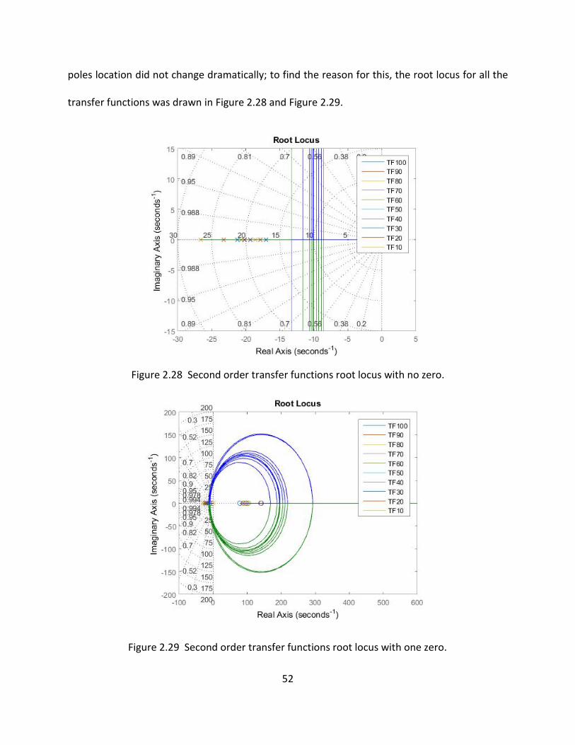
52

poles location did not change dramatically; to find the reason for this, the root locus for all the

transfer functions was drawn in Figure 2.28 and Figure 2.29.

Figure 2.29 Second order transfer functions root locus with one zero.

Figure 2.28 Second order transfer functions root locus with no zero.

53

At first glance they were quite different, but taking a closer look showed that in the region

of interest that satisfies our time domain demands, they were quite similar. Basically based on

the experiments, the overshoot had to be less than 7%, which limited us to the region between

two diagonal lines of about 0.7 damping ratio. There is no need to mention that each diagonal

line is associated with a specific damping ratio and each radial line is associated with a specific

natural frequency. Also with a vertical line, we can limit the region to the desired settling time.

So adding a zero did not help significantly with a second order transfer function.

Figure 2.30 shows that in the region of interest that the time domain demands were

satisfied, the root locus of the system with one zero, Figure 2.30, is similar to the root locus of

the system without zero in Figure 2.28.

Figure 2.30 Second order transfer functions root locus with one zero (Zoomed).

54

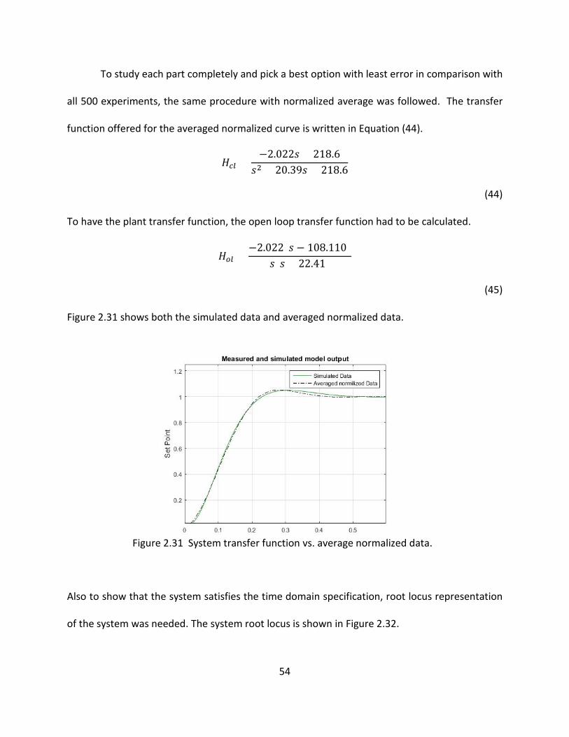
To study each part completely and pick a best option with least error in comparison with

all 500 experiments, the same procedure with normalized average was followed. The transfer

function offered for the averaged normalized curve is written in Equation (44).

𝐻𝐻𝑐𝑐𝑐𝑐 =−2.022𝑠𝑠 + 218.6

𝑠𝑠2 + 20.39𝑠𝑠 + 218.6

(44)

To have the plant transfer function, the open loop transfer function had to be calculated.

𝐻𝐻𝑜𝑜𝑐𝑐 =−2.022(𝑠𝑠 − 108.110)

𝑠𝑠(𝑠𝑠 + 22.41)

(45)

Figure 2.31 shows both the simulated data and averaged normalized data.

Also to show that the system satisfies the time domain specification, root locus representation

of the system was needed. The system root locus is shown in Figure 2.32.

Figure 2.31 System transfer function vs. average normalized data.

55

To complete this section, the matching score of this transfer function with different experiments

was calculated in Table 2-6.


with the different experiment.

As the comparison shows, adding a zero did not make a worthy contribution to the root locus, so

to find a better fit a third order system transfer function, with or without one zero, is discussed

in following section.

In the next section, also the effect of adding a pole to the transfer function is studied.


100 −2.022𝑠𝑠 + 218.6𝑠𝑠2 + 20.39𝑠𝑠 + 218.6

93.76 95.41 95.67 95.77 95.48 94.95 94.66 93.38 90.94 90.15 94.017

Figure 2.32 Root locus of system transfer function derived for average normalized data.

56

2.3 Third Order Transfer Function without Zero

Going a step further, the third order transfer function had been studied. The first and the

easiest form of transfer function of the third order is to keep the simple motor, which is in series

with an integrator. It easily solved the issue of the steady state error.

(1𝑠𝑠

) ∗𝑘𝑘𝑊𝑊𝑛𝑛

2


(46)

Thus the closed loop form corresponding to this system would be:

𝑘𝑘𝑊𝑊𝑛𝑛2

𝑠𝑠3 + 2𝜁𝜁𝑊𝑊𝑛𝑛𝑠𝑠3 + 𝑊𝑊𝑛𝑛2𝑠𝑠


𝑠𝑠3 + 2𝜁𝜁𝑊𝑊𝑛𝑛𝑠𝑠3 + 𝑊𝑊𝑛𝑛2𝑠𝑠

+ 1=


𝑠𝑠3 + 2𝜁𝜁𝑊𝑊𝑛𝑛𝑠𝑠2 + 𝑊𝑊𝑛𝑛2𝑠𝑠 + 𝑘𝑘𝑊𝑊𝑛𝑛

2

(47)

Now to make sure that the system does not have a steady state error, we used final value

theorem.

lim𝑟𝑟→0


𝑠𝑠3 + 2𝜁𝜁𝑊𝑊𝑛𝑛𝑠𝑠3 + 𝑊𝑊𝑛𝑛2𝑠𝑠 + 𝑘𝑘𝑊𝑊𝑛𝑛

2 = 1

(48)

And, to make sure that the system closed loop was also stable, Routh Horwitz criteria was helpful.

Table 2-7 Routh Hurwitz for transfer function with three poles and no zero.

Completed Routh-

Hurwitz table

57

𝑠𝑠3 1 𝑊𝑊𝑛𝑛2

𝑠𝑠2 2𝜁𝜁𝑊𝑊𝑛𝑛 𝑘𝑘𝑊𝑊𝑛𝑛2

𝑠𝑠1 − �

1 𝑊𝑊𝑛𝑛2

2𝜁𝜁𝑊𝑊𝑛𝑛 𝑘𝑘𝑊𝑊𝑛𝑛2�

2𝜁𝜁𝑊𝑊𝑛𝑛

0

To have the system stable in the Routh Hurwitz criteria, the first column of Table 2-7 had to

remain positive.

− �1 𝑊𝑊𝑛𝑛

2

2𝜁𝜁𝑊𝑊𝑛𝑛 𝑘𝑘𝑊𝑊𝑛𝑛2�

2𝜁𝜁𝑊𝑊𝑛𝑛> 0

𝑊𝑊𝑛𝑛2(2𝜁𝜁𝑊𝑊𝑛𝑛) − 𝑘𝑘𝑊𝑊𝑛𝑛

2

2𝜁𝜁𝑊𝑊𝑛𝑛> 0

𝑊𝑊𝑛𝑛

2(2𝜁𝜁) − 𝑘𝑘𝑊𝑊𝑛𝑛

2𝜁𝜁> 0

𝑊𝑊𝑛𝑛2(2𝜁𝜁) − 𝑘𝑘𝑊𝑊𝑛𝑛 > 0

2𝜁𝜁𝑊𝑊𝑛𝑛 − 𝑘𝑘 > 0

𝑘𝑘 < 2𝑊𝑊𝑛𝑛𝜁𝜁

(49)

As long as the open loop gain was less than 2𝑊𝑊𝑛𝑛𝜁𝜁, the system remained stable. This assumption

was based on the fact that the selected value for the damping ratio and natural frequency was

positive.

With this approach, first the different closed loop transfer functions regarding the

different set points were found, and they were evaluated with regard to the other curves, and

58

then the normalized averaged curve was introduced. The same procedure which had applied for

the second order was applied for the third order system.

In Table 2-8, the transfer functions which were derived with the help of Matlab

SystemIdentification tools were tested with other experimental data to find the rate of matching

regarding each pair.

Table 2-8 Matching score of the different transfer functions with 3 poles and no zero comparing with the different experiments.

Looking at Table 2-8, it is clear that an improvement has been made in comparison with

the second order transfer function representation.


100 4481

𝑠𝑠3 + 34.79𝑠𝑠2 + 543.4𝑠𝑠 + 4481 96.88 97.73 97.24 96.36 94.95 95.37 94.99 93.4 90.59 88.51 94.602

90 3938

𝑠𝑠3 + 32.83𝑠𝑠2 + 512𝑠𝑠 + 3938 96.6 98.18 97.97 97.33 95.82 96.05 95.62 94.03 91.16 89.28 95.204

80 4169

𝑠𝑠3 + 33.03𝑠𝑠2 + 533.5𝑠𝑠 + 4169 96.25 97.96 98.19 97.79 96.5 96.77 96.26 94.82 91.81 89.97 95.632

70 3880

𝑠𝑠3 + 31.62𝑠𝑠2 + 515.2𝑠𝑠 + 3880 95.66 97.46 97.97 98.01 96.97 97.12 96.56 95.28 92.23 90.51 95.777

60 4610

𝑠𝑠3 + 32.85𝑠𝑠2 + 576.8𝑠𝑠 + 4609 94.76 96.36 97.13 97.56 97.37 97.51 96.81 96.22 92.95 91.52 95.819

50 5068

𝑠𝑠3 + 33.3𝑠𝑠2 + 597.5𝑠𝑠 + 5067 95.12 96.45 97.18 97.34 97.18 97.71 96.94 96.38 92.95 91.3 95.855

40 4794

𝑠𝑠3 + 32.51𝑠𝑠2 + 576.2𝑠𝑠 + 4794 95.17 96.56 97.29 97.46 97.2 97.7 96.94 96.29 92.91 91.2 95.872

30 5835

𝑠𝑠3 + 34.79𝑠𝑠2 + 647.9𝑠𝑠 + 5835 93.91 94.9 95.72 96.05 96.62 97.13 96.39 96.84 93.26 92.06 95.288

20 4726

𝑠𝑠3 + 29.97𝑠𝑠2 + 569.3𝑠𝑠 + 4726 93.55 94.82 95.67 96.25 96.73 96.95 96.28 96.69 93.32 92.08 95.234

10 9085𝑠𝑠3 + 39.94𝑠𝑠2 + 928.5𝑠𝑠 + 9085 91.21 92.03 92.97 93.43 94.47 94.32 93.67 94.72 91.88 93.41 93.211

59

To study the case closer let us take a look over the pole zero map of each of the transfer

functions in Figure 2.33.

As can be seen in Figure 2.33, all poles of the closed loop system are located near each other.

However, our plant was the open loop system, thus we needed to extract the open loop system

transfer function.

Figure 2.33 Pole zero representation of closed loop transfer function with 3 poles and

no zeros.

60

Table 2-9 Poles in a closed loop form.

S.P Transfer function Poles beside integrator

100 4481

𝑠𝑠3 + 34.79𝑠𝑠2 + 543.4𝑠𝑠 + 4481 -17.3950 ±15.5182i

90 3938

𝑠𝑠3 + 32.83𝑠𝑠2 + 512𝑠𝑠 + 3938 -16.4150 ±15.5739i

80 4169

𝑠𝑠3 + 33.03𝑠𝑠2 + 533.5𝑠𝑠 + 4169 -16.5150 ±16.1479i

70 3880

𝑠𝑠3 + 31.62𝑠𝑠2 + 515.2𝑠𝑠 + 3880 -15.8100 ±16.2863i

60 4610

𝑠𝑠3 + 32.85𝑠𝑠2 + 576.8𝑠𝑠 + 4609 -16.4250 ±17.5220i

50 5068𝑠𝑠3 + 33.3𝑠𝑠2 + 597.5𝑠𝑠 + 5067

-16.6500 ±17.8963i

40 4794

𝑠𝑠3 + 32.51𝑠𝑠2 + 576.2𝑠𝑠 + 4794 -16.2550 ±17.6628i

30 5835

𝑠𝑠3 + 34.79𝑠𝑠2 + 647.9𝑠𝑠 + 5835 -17.3950 ±18.5826i

20 4726

𝑠𝑠3 + 29.97𝑠𝑠2 + 569.3𝑠𝑠 + 4726 -14.9850 ±18.5674i

10 9085𝑠𝑠3 + 39.94𝑠𝑠2 + 928.5𝑠𝑠 + 9085

-19.9700 ±23.0152i

Table 2-9 shows that the real part of the open loop poles swings in the small region but

the imaginary part is decreased. The reason is that the real part of the open loop system is

responsible for damping and the imaginary part is responsible for the duration of each overshoot

and undershoot. By changing the real part of the open loop, the system overshoot is changed,

and by increasing the amplitude of the imaginary part of the pole, the duration of the overshoot

is decreased.

To better understand let us take a look over the system root locus in Figure 2.34.

61

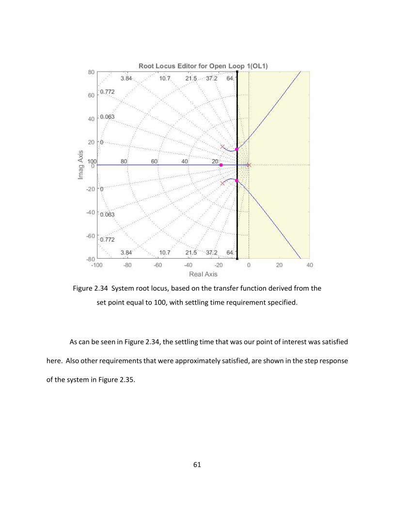
As can be seen in Figure 2.34, the settling time that was our point of interest was satisfied

here. Also other requirements that were approximately satisfied, are shown in the step response

of the system in Figure 2.35.

Figure 2.34 System root locus, based on the transfer function derived from the

set point equal to 100, with settling time requirement specified.

62

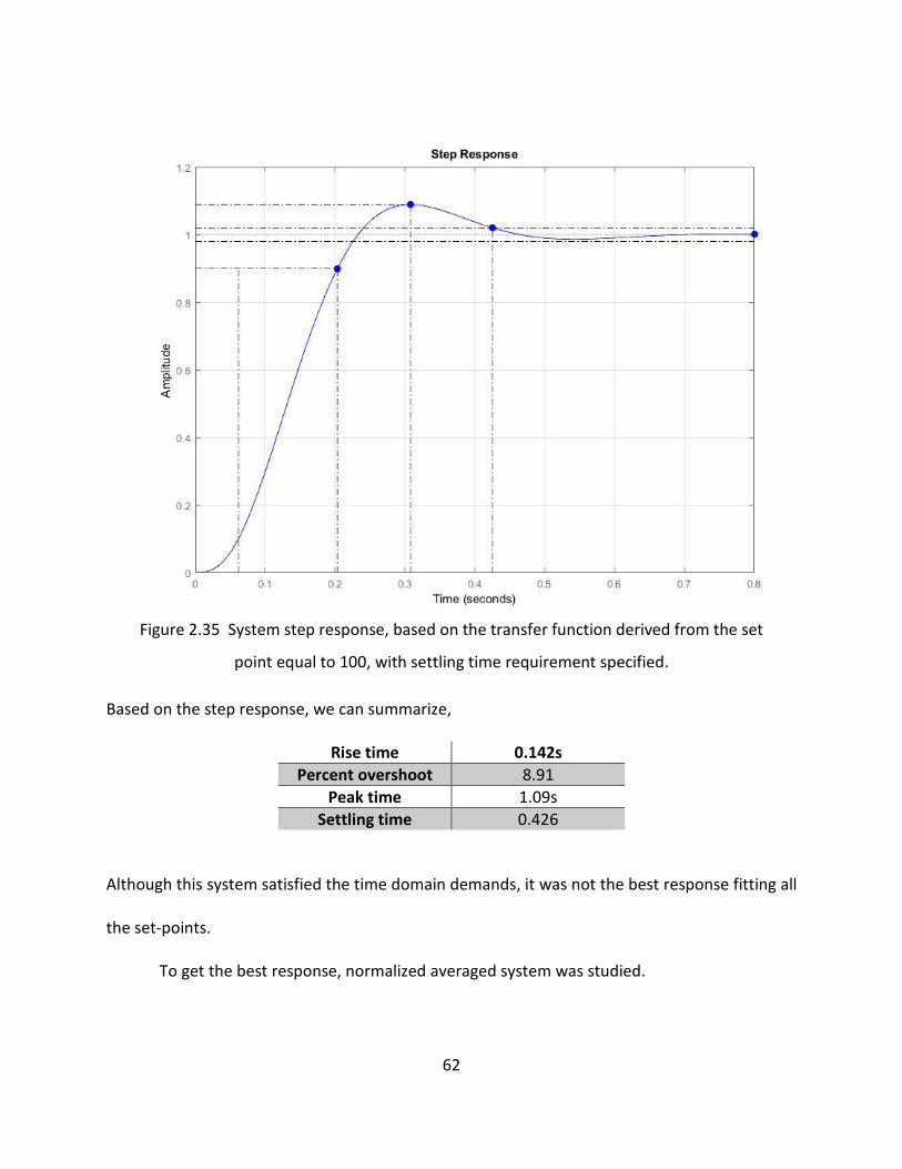
Based on the step response, we can summarize,

Rise time 0.142s Percent overshoot 8.91

Peak time 1.09s Settling time 0.426

Although this system satisfied the time domain demands, it was not the best response fitting all

the set-points.

To get the best response, normalized averaged system was studied.

Figure 2.35 System step response, based on the transfer function derived from the set

point equal to 100, with settling time requirement specified.

63

Table 2-10 Matching rate of the final transfer functions with 3 poles and no zero comparing with the different experiment.

By using Matlab system-identification tool, least square estimation method, we could

evaluate how much this transfer function fit different experiments. As shown in Table 2-10, using

the averaged normalized data gave a better fit to all experiments so far.

The open loop representation for the system is,

5036𝑠𝑠3 + 35.98𝑠𝑠2 + 623.4𝑠𝑠

(50)

Equation (50) is the plant transfer function in third order type. To go a step further, third order

system with one zero also is discussed in the next section.

S.P Transfer function Ave 100 90 80 70 60 50 40 30 20 10 Ave.

Ave 5036

𝑠𝑠3 + 35.98𝑠𝑠2 + 623.4𝑠𝑠 + 5036 98.82 95.02 96.7 97.41 97.74 97.25 97.25 96.62 95.8 92.66 91.35 96.527

64

2.4 Third Order Transfer Function with One Zero

To study the system more carefully, let us study the case with a transfer function with 3

poles and one zero.

𝐻𝐻𝑜𝑜𝑐𝑐(𝑠𝑠) =𝑊𝑊𝑛𝑛

2(𝑠𝑠 + 𝑧𝑧1)𝑠𝑠3 + 2𝜁𝜁𝑊𝑊𝑛𝑛𝑠𝑠2 + 𝑊𝑊𝑛𝑛

2𝑠𝑠

(51)

By using Equation (51), the close loop could be derived.

𝐻𝐻𝑐𝑐𝑐𝑐(𝑠𝑠) =(𝑠𝑠 + 𝑧𝑧1) ∗ 𝑊𝑊𝑛𝑛

2

𝑠𝑠3 + 2𝜁𝜁𝑊𝑊𝑛𝑛𝑠𝑠2 + 𝑊𝑊𝑛𝑛2𝑠𝑠 + (𝑠𝑠 + 𝑧𝑧1) ∗ 𝑊𝑊𝑛𝑛

2 =(𝑠𝑠 + 𝑧𝑧1) ∗ 𝑊𝑊𝑛𝑛

2

𝑠𝑠3 + 2𝜁𝜁𝑊𝑊𝑛𝑛𝑠𝑠2 + 2𝑊𝑊𝑛𝑛2𝑠𝑠 + 𝑧𝑧1𝑊𝑊𝑛𝑛

2

(52)

Achieving the closed loop transfer function allowed us to find the steady state error using final

value theorem (Equation (53)).

lim𝑟𝑟→0

(𝑠𝑠 + 𝑧𝑧1) ∗ 𝑊𝑊𝑛𝑛2

𝑠𝑠3 + 2𝜁𝜁𝑊𝑊𝑛𝑛𝑠𝑠2 + 2𝑊𝑊𝑛𝑛2𝑠𝑠 + 𝑧𝑧1𝑊𝑊𝑛𝑛

2 =𝑧𝑧1𝑊𝑊𝑛𝑛

2

𝑧𝑧1𝑊𝑊𝑛𝑛2 = 1

(53)

The same path which had been followed to find the region of stability for the third order closed

loop system without a zero had to be followed for the system closed loop transfer function with

a zero. A general third order system with one zero has the following form (Equation (54)).

65

𝐻𝐻𝑜𝑜𝑐𝑐(𝑠𝑠) =𝐾𝐾(𝑠𝑠 + 𝑧𝑧1)

𝑠𝑠3 + 𝑎𝑎𝑠𝑠2 + 𝑏𝑏𝑠𝑠 + 𝑐𝑐

(54)

The corresponding closed loop system is described with the following equation (Equation (55)).

𝐻𝐻𝑐𝑐𝑐𝑐(𝑠𝑠) =𝐾𝐾(𝑠𝑠 + 𝑧𝑧1)

𝑠𝑠3 + 𝑎𝑎𝑠𝑠2 + (𝑏𝑏 + 𝐾𝐾)𝑠𝑠 + 𝑐𝑐 + 𝐾𝐾𝑧𝑧1

(55)

The first issue to be addressed was the Routh-Horwitz table, to find the region of stability.

Table 2-11 Routh Hurwitz for transfer function with 3 poles and one zero.

Completed Routh-

Hurwitz table

𝑠𝑠3 1 b+𝐾𝐾

𝑠𝑠2 a c+𝐾𝐾𝑧𝑧1

𝑠𝑠1

− �1 b + 𝐾𝐾𝑎𝑎 c + 𝐾𝐾𝑧𝑧1

�

𝑎𝑎

= 𝑖𝑖

0

Based on Table 2-11, “f” had to be positive, to make the whole system stable.

− �1 b + 𝐾𝐾𝑎𝑎 c + 𝐾𝐾𝑧𝑧1

�

𝑎𝑎= 𝑖𝑖

(56)

To simplify the calculation, the following variable changes were used:

66

𝑏𝑏′ = (𝑏𝑏 + 𝐾𝐾)

𝑐𝑐′ = 𝑐𝑐 + 𝐾𝐾𝑧𝑧1

(57)

By plugging those values into the general equation, we obtained,

𝐻𝐻𝑐𝑐𝑐𝑐(𝑠𝑠) =𝐾𝐾(𝑠𝑠 + 𝑧𝑧1)

𝑠𝑠3 + 𝑎𝑎𝑠𝑠2 + 𝑏𝑏′𝑠𝑠 + 𝑐𝑐′

(58)

The characteristic equation of the closed loop system is the denominator of Equation (58):

𝑠𝑠3 + 𝑎𝑎𝑠𝑠2 + 𝑏𝑏′𝑠𝑠 + 𝑐𝑐′

(59)

The roots of characteristic equation are poles of the system that determine the shape of the

system. Unfortunately, the roots of the third order system cannot be studied directly due to the

fact that the roots are too complex. So, instead of a direct approach, an indirect approach to

study the roots of third order system had been used.

To go through an indirect study, the value for ∆ had to be calculated and based on that

value, the root location can be estimated.

∆= 18𝑎𝑎𝑏𝑏𝑐𝑐 − 4𝑎𝑎3𝑐𝑐 + 𝑎𝑎2𝑏𝑏2 − 4𝑏𝑏3 − 27𝑐𝑐2

(60)

If ∆>0, then the equation has three distinct real poles.

If ∆=0, then the equation has triple real poles. .

If ∆<0, then the equation has a real pole and a complex conjugate pole.

Considering the general characteristic equation was equal to zero:

67

𝑠𝑠3 + 𝑎𝑎𝑠𝑠2 + 𝑏𝑏′𝑠𝑠 + 𝑐𝑐′ = 0

(61)

The roots could be found by using the following equation (Equation (62)):

𝑝𝑝𝑘𝑘 = −1

3𝑎𝑎�𝑏𝑏 + 𝑢𝑢𝑘𝑘𝐶𝐶 +

∆0𝑢𝑢𝑘𝑘𝐶𝐶

� , 𝑘𝑘 ∈ {1,2,3}

(62)

In Equation (62), some unknown variables had been used whose values are introduced in

following equations (63-66).

Where:

𝑢𝑢1 = 1,𝑢𝑢2 =−1 + 𝑗𝑗√3

2,𝑢𝑢3 =

−1 − 𝑗𝑗√32

(63)

And

𝐶𝐶 = �∆1 + �∆12 − 4∆03

2

3

(64)

∆0= 𝑎𝑎2 − 3𝑏𝑏

(65)

∆1= 2𝑎𝑎3 − 9𝑎𝑎𝑏𝑏 + 27𝑐𝑐

(66)

Different cases may have different inverse Laplace transform; here is the calculated inverse

Laplace for all of the cases.

68

1. 3 real poles:

𝐾𝐾(𝑠𝑠 + 𝑧𝑧1)𝑠𝑠3 + 𝑎𝑎𝑠𝑠2 + 𝑏𝑏′𝑠𝑠 + 𝑐𝑐′

=𝐾𝐾(𝑠𝑠 + 𝑧𝑧1)

(𝑠𝑠 + 𝑝𝑝1)(𝑠𝑠 + 𝑝𝑝2)(𝑠𝑠 + 𝑝𝑝3)=

𝐴𝐴𝑠𝑠 + 𝑝𝑝1

+𝐵𝐵

𝑠𝑠 + 𝑝𝑝2+

𝐶𝐶𝑠𝑠 + 𝑝𝑝3

𝐴𝐴 =𝐾𝐾(−𝑝𝑝1 + 𝑧𝑧1)

(−𝑝𝑝1 + 𝑝𝑝2)(−𝑝𝑝1 + 𝑝𝑝3)

𝐵𝐵 =𝐾𝐾(−𝑝𝑝2 + 𝑧𝑧1)

(−𝑝𝑝2 + 𝑝𝑝1)(−𝑝𝑝2 + 𝑝𝑝3)

𝐶𝐶 =𝐾𝐾(−𝑝𝑝3 + 𝑧𝑧1)

(−𝑝𝑝3 + 𝑝𝑝1)(−𝑝𝑝3 + 𝑝𝑝2)

ℒ−1 �𝐾𝐾(𝑠𝑠 + 𝑧𝑧1)

(𝑠𝑠 + 𝑝𝑝1)(𝑠𝑠 + 𝑝𝑝2)(𝑠𝑠 + 𝑝𝑝3)� = ℒ−1 �


� + ℒ−1 �𝐵𝐵

𝑠𝑠 + 𝑝𝑝2� + ℒ−1 �

𝐶𝐶𝑠𝑠 + 𝑝𝑝3

�

= 𝐴𝐴𝑒𝑒−𝑝𝑝1𝑑𝑑 + 𝐵𝐵𝑒𝑒−𝑝𝑝2𝑑𝑑 + 𝐶𝐶𝑒𝑒−𝑝𝑝3𝑑𝑑

(67)

As this system only had real pole, there was not any overshoot. Thus this did not fit the curve.

2. One triple root:


=𝐾𝐾(𝑠𝑠 + 𝑧𝑧1)(𝑠𝑠 + 𝑝𝑝1)3

ℒ−1 �𝐾𝐾(𝑠𝑠 + 𝑧𝑧1)

(𝑠𝑠 + 𝑝𝑝1)(𝑠𝑠 + 𝑝𝑝2)(𝑠𝑠 + 𝑝𝑝3)� = ℒ−1 �𝐾𝐾(𝑠𝑠 + 𝑧𝑧1)(𝑠𝑠 + 𝑝𝑝1)3�

= ℒ−1 �𝐾𝐾𝑠𝑠

(𝑠𝑠 + 𝑝𝑝1)3� + ℒ−1 �𝐾𝐾𝑧𝑧1

(𝑠𝑠 + 𝑝𝑝1)3�

=𝐾𝐾2∗𝑑𝑑𝑑𝑑𝑡𝑡

(𝑡𝑡2𝑒𝑒−𝑝𝑝1𝑑𝑑) +𝐾𝐾𝑧𝑧1

2(𝑡𝑡2𝑒𝑒−𝑝𝑝1𝑑𝑑) =

𝐾𝐾2𝑒𝑒−𝑝𝑝1𝑑𝑑(2𝑡𝑡 − 𝑝𝑝1𝑡𝑡2) +

𝐾𝐾𝑧𝑧12

(𝑡𝑡2𝑒𝑒−𝑝𝑝1𝑑𝑑)

(68)

69

Due to existence of the term “t”, it was not stable and could not fit the system.

3. One real pole and a pair of complex conjugate form


=𝐾𝐾(𝑠𝑠 + 𝑧𝑧1)

(𝑠𝑠 + 𝑝𝑝1)(𝑠𝑠 + 𝑝𝑝2)(𝑠𝑠 + 𝑝𝑝3)=


+𝐵𝐵

𝑠𝑠 + 𝑝𝑝2+

𝐵𝐵�𝑠𝑠 + 𝑝𝑝2��


(−𝑝𝑝1 + 𝑝𝑝2)(−𝑝𝑝1 + 𝑝𝑝2��)


(−𝑝𝑝2 + 𝑝𝑝1)(−𝑝𝑝2 + 𝑝𝑝2��)

𝐵𝐵� =𝐾𝐾(−𝑝𝑝2��+ 𝑧𝑧1)

(−𝑝𝑝2��+ 𝑝𝑝1)(−𝑝𝑝2��+ 𝑝𝑝2)

(69)

To simplify the calculation, we assumed that (Equation (70)).

𝑝𝑝2 = 𝑛𝑛 + 𝑗𝑗𝑗𝑗

𝑝𝑝2 = 𝑛𝑛 − 𝑗𝑗𝑗𝑗

(70)

By substituting these values into Equation (58) and using partial fraction decomposition, the

coefficient for the fraction could be derived as in the following equations (Equation (71) and

Equation (72)).


(−𝑝𝑝1 + 𝑝𝑝2)(−𝑝𝑝1 + 𝑝𝑝2��)=

𝐾𝐾(−𝑝𝑝1 + 𝑧𝑧1)(−𝑝𝑝1 + 𝑛𝑛 + 𝑗𝑗𝑗𝑗)(−𝑝𝑝1 + 𝑛𝑛 − 𝑗𝑗𝑗𝑗)

=𝐾𝐾(−𝑝𝑝1 + 𝑧𝑧1)

(−𝑝𝑝1 + 𝑛𝑛)2 + 𝑗𝑗2

(71)

70


(−𝑝𝑝2 + 𝑝𝑝1)(−𝑝𝑝2 + 𝑝𝑝2��)=

𝐾𝐾(−(𝑛𝑛 + 𝑗𝑗𝑗𝑗) + 𝑧𝑧1)(−(𝑛𝑛 + 𝑗𝑗𝑗𝑗) + 𝑝𝑝1)(−(𝑛𝑛 + 𝑗𝑗𝑗𝑗) + 𝑝𝑝2��)

=𝐾𝐾(−(𝑛𝑛 + 𝑗𝑗𝑗𝑗) + 𝑧𝑧1)

(−(𝑛𝑛 + 𝑗𝑗𝑗𝑗) + 𝑝𝑝1)(−(𝑛𝑛 + 𝑗𝑗𝑗𝑗) + 𝑛𝑛 − 𝑗𝑗𝑗𝑗)=

𝐾𝐾(𝑧𝑧1 − 𝑛𝑛 − 𝑗𝑗𝑗𝑗)(𝑝𝑝1 − 𝑛𝑛 − 𝑗𝑗𝑗𝑗)(−2𝑗𝑗𝑗𝑗)

=𝐾𝐾(𝑧𝑧1 − 𝑛𝑛 − 𝑗𝑗𝑗𝑗)

(−2𝑗𝑗𝑗𝑗)(𝑝𝑝1 − 𝑛𝑛) − 2𝑗𝑗2 ∗(+2𝑗𝑗𝑗𝑗)(𝑝𝑝1 − 𝑛𝑛) − 2𝑗𝑗2

(+2𝑗𝑗𝑗𝑗)(𝑝𝑝1 − 𝑛𝑛) − 2𝑗𝑗2

=𝐾𝐾(𝑧𝑧1 − 𝑛𝑛 − 𝑗𝑗𝑗𝑗) ∗ (+2𝑗𝑗𝑗𝑗)(𝑝𝑝1 − 𝑛𝑛) − 2𝑗𝑗2

4𝑗𝑗4 + 4𝑗𝑗2(𝑝𝑝1 − 𝑛𝑛)

(72)

First the transfer function for each of the experiments was calculated with Matlab

systemIdentification tool. Later on the root locus of the system was discussed to see the zero

contribution to the time domain demands were satisfied; and finally to find the best fit for all the

experiments, the averaged normalized time domain experiment was examined.

Table 2-12 shows the transfer function derived from the experiment, and also the

matching score associated with them is in comparison with each of the experiments.

71

Table 2-12 Matching rate of the final transfer functions with 3 poles and one zero comparing with the different experiment.

S.P Transfer function 100 90 80 70 60 50 40 30 20 10 Ave.

100 116.1𝑠𝑠 + 4488

𝑠𝑠3 + 34.83𝑠𝑠2 + 544𝑠𝑠 + 4488 96.88 97.73 97.24 96.36 94.95 95.37 94.99 93.4 90.59 88.51 94.602

90 96.12𝑠𝑠 + 3945𝑠𝑠3 + 32.87𝑠𝑠2 + 512.6𝑠𝑠 + 3945

96.6 98.18 97.97 97.33 95.82 96.05 95.62 94.03 91.16 89.28 95.204

80 107.1𝑠𝑠 + 4170

𝑠𝑠3 + 33.04𝑠𝑠2 + 533.5𝑠𝑠 + 4170 96.25 97.96 98.19 97.79 96.5 96.77 96.26 94.82 91.81 89.97 95.632

70 108.6𝑠𝑠 + 3889

𝑠𝑠3 + 31.66𝑠𝑠2 + 516.1𝑠𝑠 + 3889 95.66 97.45 97.97 98.01 96.97 97.13 96.56 95.29 92.23 90.51 95.778

60 119.2𝑠𝑠 + 4615

𝑠𝑠3 + 32.87𝑠𝑠2 + 577.2𝑠𝑠 + 4615 94.76 96.36 97.13 97.56 97.37 97.51 96.81 96.23 92.95 91.53 95.821

50 106.9𝑠𝑠 + 5070𝑠𝑠3 + 33.31𝑠𝑠2 + 597.5𝑠𝑠 + 5070

95.12 96.45 97.18 97.33 97.18 97.71 96.94 96.38 92.95 91.3 95.854

40 109.8𝑠𝑠 + 4781

𝑠𝑠3 + 32.46𝑠𝑠2 + 575.1𝑠𝑠 + 4781 95.17 96.56 97.29 97.47 97.2 97.7 96.94 96.29 92.91 91.2 95.873

30 90.9𝑠𝑠 + 5840

𝑠𝑠3 + 33.22𝑠𝑠2 + 648.3𝑠𝑠 + 5840 93.91 94.9 95.72 96.05 96.62 97.13 96.38 96.84 93.25 92.07 95.287

20 172.9𝑠𝑠 + 4755𝑠𝑠3 + 30.05𝑠𝑠2 + 571.4𝑠𝑠 + 4755

93.55 94.83 95.67 96.25 96.73 96.95 96.28 96.7 93.32 92.09 95.237

10 116.1𝑠𝑠 + 9041

𝑠𝑠3 + 39.84𝑠𝑠2 + 925.2𝑠𝑠 + 9041 91.22 92.04 92.98 93.45 94.48 94.32 93.68 94.73 91.89 93.41 93.22

As we can see from Table 2-12, adding a zero did not make a significant improvement in

the system. The transfer function regarding the averaged normalized data also had been

calculated.

Table 2-13 Matching rate of the averaged normalized form with 3 poles and one zero comparing with the different experiment.

S.P Transfer function 100 90 80 70 60 50 40 30 20 10 Ave.

Ave 116.1𝑠𝑠 + 5036𝑠𝑠3 + 35.98𝑠𝑠2 + 623.4𝑠𝑠 + 5036

95.02 96.7 97.41 97.74 97.25 97.25 96.62 95.8 92.66 91.35 95.78

72

Using the averaged normalized form of the time domain representation gave us a better transfer

function which fit the different experiments more.

Comparing the two recent Table 2-10 and Table 2-13 shows that adding a zero did not

make a significant contribution. To find the reason we compared the two pole zero map for both

series of the closed loop transfer functions in Figure 2.36 and Figure 2.37.

Figure 2.36 Pole zero constellations for a third order transfer function without zero.

73

Considering these two closed loop system, it appeared that the closed loop poles that are

responsible for time domain behavior had not been relocated. To study it more precisely, we

derived the system open loop transfer function by its open loop poles and zeros and the root

locus.

Figure 2.37 Pole zero constellation for a third order transfer function with one zero.

74

Table 2-14 Open loop poles and zeros.

S.P Transfer function OL TF OL poles OL zeros

100 116.1𝑠𝑠 + 4488

𝑠𝑠3 + 34.83𝑠𝑠2 + 544𝑠𝑠 + 4488

116.1𝑠𝑠 + 4488𝑠𝑠3 + 34.83𝑠𝑠2 + 427.9𝑠𝑠

-17.4150 +11.1632i -38.6563

90 96.12𝑠𝑠 + 3945𝑠𝑠3 + 32.87𝑠𝑠2 + 512.6𝑠𝑠 + 3945

96.12𝑠𝑠 + 3945

𝑠𝑠3 + 32.87𝑠𝑠2 + 416.48𝑠𝑠 -16.4350 +12.0984i -40.0424

80 107.1𝑠𝑠 + 4170

𝑠𝑠3 + 33.04𝑠𝑠2 + 533.5𝑠𝑠 + 4170

107.1𝑠𝑠 + 4170𝑠𝑠3 + 33.04𝑠𝑠2 + 426.4𝑠𝑠

-16.5200 +12.3891i -38.9356

70 108.6𝑠𝑠 + 3889

𝑠𝑠3 + 31.66𝑠𝑠2 + 516.1𝑠𝑠 + 3889

108.6𝑠𝑠 + 3889𝑠𝑠3 + 31.66𝑠𝑠2 + 407.5𝑠𝑠

-15.8300 +12.5264i -35.8103

60 119.2𝑠𝑠 + 4615

𝑠𝑠3 + 32.87𝑠𝑠2 + 577.2𝑠𝑠 + 4615

119.2𝑠𝑠 + 4615𝑠𝑠3 + 32.87𝑠𝑠2 + 458𝑠𝑠

-16.4350 +13.7073i -38.7164

50 106.9𝑠𝑠 + 5070

𝑠𝑠3 + 33.31𝑠𝑠2 + 597.5𝑠𝑠 + 5070

106.9𝑠𝑠 + 5070𝑠𝑠3 + 33.31𝑠𝑠2 + 490.6𝑠𝑠

-16.6550 +14.6017i -47.4275

40 109.8𝑠𝑠 + 4781

𝑠𝑠3 + 32.46𝑠𝑠2 + 575.1𝑠𝑠 + 4781

109.8𝑠𝑠 + 4781𝑠𝑠3 + 32.46𝑠𝑠2 + 465.3𝑠𝑠

-16.2300 +14.2087i -43.5428

30 90.9𝑠𝑠 + 5840

𝑠𝑠3 + 33.22𝑠𝑠2 + 648.3𝑠𝑠 + 5840

90.9𝑠𝑠 + 5840𝑠𝑠3 + 33.22𝑠𝑠2 + 557.4𝑠𝑠

-16.1100 +17.2588i -64.2464

20 172.9𝑠𝑠 + 4755

𝑠𝑠3 + 30.05𝑠𝑠2 + 571.4𝑠𝑠 + 4755

172.9𝑠𝑠 + 4755𝑠𝑠3 + 30.05𝑠𝑠2 + 398.5𝑠𝑠

-15.0250 +13.1434i -27.5014

10 116.1𝑠𝑠 + 9041

𝑠𝑠3 + 39.84𝑠𝑠2 + 925.2𝑠𝑠 + 9041

116.1𝑠𝑠 + 9041𝑠𝑠3 + 39.84𝑠𝑠2 + 809.1𝑠𝑠

-19.9200 +20.3050i -77.8725

The plant poles showed that there was little relocation between plant systems with and without

a zero. To find out why, we compared both systems’ root locus presentation in Figure 2.38 and

Figure 2.39.

75

As seen in Figure 2.38 and Figure 2.39 adding a zero did not affect the root locus in the

stable region, which means the time domain behavior of the system did not change effectively.

Figure 2.38 Plant root locus with 3 poles and one zero.

Figure 2.39 Plant root locus with 3 poles and no zero.

76

In the following figure, both transfer function and the averaged normalized curve are

depicted in one frame (Figure 2.40).

As shown in Figure 2.40, there is little improvement between the transfer function derived with

zero and the one derived without zero.

Figure 2.40 Simulated data and averaged normalized data.

77

3. CHAPTER 3

CONCLUSION

The system that grabbed our attention was the new generation of Lego Mindstorms

series, named LEGO EV3. To use this device in academia, the transfer function of the system

needed to be derived precisely.

In this study, two different types of transfer function were derived from the same plant;

first the second order transfer function was tested in the system. Studying the system in both

situations, with and without zero, showed that adding a zero to a second order system did not

make a contribution. Further studies showed that the plant had a built-in Integrator, which

eliminated the steady states error.

The second order transfer function of this system had the following equation.

𝐻𝐻𝑜𝑜𝑐𝑐 =218.6

𝑠𝑠2 + 20.39𝑠𝑠

(72)

Comparing the simulation result with the experimental data showed that this transfer function

matches the data for 94.017 %. In comparison all the set-points had been considered. Putting a

step forward, after being disappointed with adding a zero, a pole had been added to the transfer

function.

The result for a transfer function with 3 poles and no zero follows.

𝐻𝐻𝑜𝑜𝑐𝑐 =5036

𝑠𝑠3 + 35.98𝑠𝑠2 + 623.4𝑠𝑠

(73)

78

Simulating this transfer function and comparing the results with the experimental data shows

that this transfer function matches the experiments with the rate of 96.5 %.

For future work, considering the fraction and saturation as two main disturbances can be

offered. As in this work, for simplicity, the fraction had been eliminated. As the user puts the

robot on a surface, the fraction would affect the transfer function. Changing the surface changes

the friction coefficient. This study also focused on linear region which at most rotates the wheels

for 100 degrees, higher value which were in saturation region had not been studied in this work.

79

REFERENCES

[1] C. D. Vries et al, “Using LEGO MINDSTORMS in a Control Systems Lab to impact next

generation engineers,” in 122nd ASEE annual conf., Seattle., WA, 2015,

[2] V. Sood et al, “Establishing a cost effective control and robotics program: Delay based wireless

feedback control using LEGO's,” in Integrated STEM Education Conference (ISEC), IEEE.,

Princeton., NJ, 2015, pp. 210-215.

[3] H. S. Chuang et al, “Development of a low-cost platform for control engineering education,”

in International Conference on Machine Learning and Cybernetics., Lanzhou, 2014, pp. 444-448.

[4] R. Jain et al, “Establishing a cost effective embedded control and robotics engineering

program, Observer based state feedback control using LEGOs,” in Integrated STEM Education

Conference (ISEC), IEEE., Princeton., NJ, 2013, pp. 1-6.

[5] S. A. Wadoo et al, “A Lego based undergraduate control systems Laboratory,” in Systems,

Applications and Technology Conference (LISAT), IEEE., Farmingdale, NY, 2012, pp. 1-6.

[6] M. Canale et al, “A Lego Mindstorms NXT experiment for Model Predictive Control education,”

in Control Conference (ECC), Zurich, 2013, pp. 2549-2554.

[7] H. Nanal et al, “Establishing a cost effective embedded control and robotics engineering

program optimal control of a two wheeled robot,” in Systems, Applications and Technology

Conference (LISAT), IEEE., Farmingdale, NY, 2013, pp. 1-6.

[8] R. Sugumaran et al, “Establishing a cost effective embedded control and robotics engineering

program,Linear optimal control design using LEGOs,” in Integrated STEM Education Conference

(ISEC), IEEE., Princeton., NJ, 2013, pp. 1-6.

80

[9] P. J. Bradley et al, “A Platform for Real-Time Control Education with LEGO MINDSTORMSR,”

in 9th IFAC Symposium Advances in Control Education The International Federation of Automatic

Control, Nizhny Novgorod, Russia, 2012, pp. 112-117.

[10] J. M. Gómez-de-Gabriel et al, “Using LEGO NXT Mobile Robots With LabVIEW,” in IEEE

TRANSACTIONS ON EDUCATION, VOL. 54, NO. 1, 2011, pp. 41-47.

[11] Y. Kim, “Control systems lab using a LEGO Mindstorms NXT motor system,” in 18th

Mediterranean Conference on Control & Automation., Marrakech, Morocco, 2010, pp. 452-461.

[12] Y. Kim, “Control systems lab using a LEGO Mindstorms NXT motor system,” in IEEE

TRANSACTIONS ON EDUCATION, VOL. 54, NO. 3., 2011, pp. 452-461.

[13] A. Pilat et al, Inter-university Project Based on LEGO NXT,” in Control Applications, (CCA) &

Intelligent Control, (ISIC), IEEE., St. Petersburg, 2009, pp. 1248-1253.

[14] W. Grega et al, “Real-time control teaching using LEGO® MINDSTORMS® NXT robot” in

Computer Science and Information Technology, Wisia, 2008, pp. 625-628.

[15] S. H. Kim et al, “Introduction for Freshmen to Embedded Systems,” in IEEE TRANSACTIONS

ON EDUCATION, VOL. 52, NO. 1, 2009, pp. 99-108.

[16] N. Z. Azlan, “Fuzzy Logic Controlled Miniature LEGO Robot for Undergraduate Training

System,” in 2nd IEEE Conference on Industrial Electronics and Applications. Harbon, 2007, pp.

2184-2188.

[17] E. Wang et al, “Using LEGO bricks to conduct engineering experiment,” in American Society

for Engineering Education Annual Conference & Exposition, 2004

[18] “A LEGO-Based control experiment,” in IEEE Control Systems Magazine, 2004, p43-56

[19] Matlab and Simulink. Math works [Online]. Available: www.mathworks.com

81

[20] J. F. Franklin, Feedback control, Dynamic system. Prentice Hall, NJ, 2002.

The Modeling and Simulation of EV3 Motor Dynamics/67531/metadc862751/m2/1/high... · Lego...

Documents

Transcript of The Modeling and Simulation of EV3 Motor Dynamics/67531/metadc862751/m2/1/high... · Lego...