1

15.053/8 April 23, 2013

The Minimum Cost Flow Problem

2

Quotes of the day

“A process cannot be understood by stopping it. Understanding must move with the flow of the process, must join it and flow with it.”

-- Frank Herbert “No question is so difficult to answer as that to

which the answer is obvious.” -- George Bernard Shaw

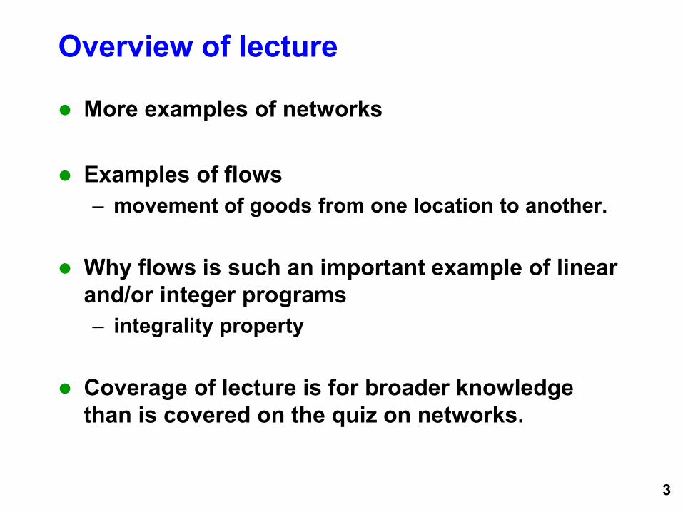
Overview of lecture

More examples of networks Examples of flows

– movement of goods from one location to another.

Why flows is such an important example of linear and/or integer programs – integrality property

Coverage of lecture is for broader knowledge

than is covered on the quiz on networks.

3

Networks are everywhere

Physical networks

Time space networks

Connections between concepts

Social networks

Network flows: model movements in networks

4

5

Road Network

Power Grid Boston MBTA Train Map

Electrical Network Photo courtesy of Derrick Coetzee on Flickr.

Image removed due to copyright restrictions.

Public domain image (EIA.gov)

Public domain image (Wikimedia Commons)

6

Internet from wikipedia

Courtesy of the Opte Project, License CC BY.

7

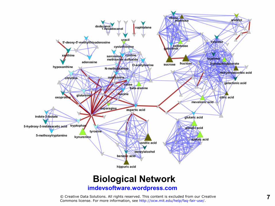
Biological Network imdevsoftware.wordpress.com

© Creative Data Solutions. All rights reserved. This content is excluded from our CreativeCommons license. For more information, see http://ocw.mit.edu/help/faq-fair-use/.

8

Biological neural network

Public domain (NIH)

Computer neural network

Public domain (NASA)

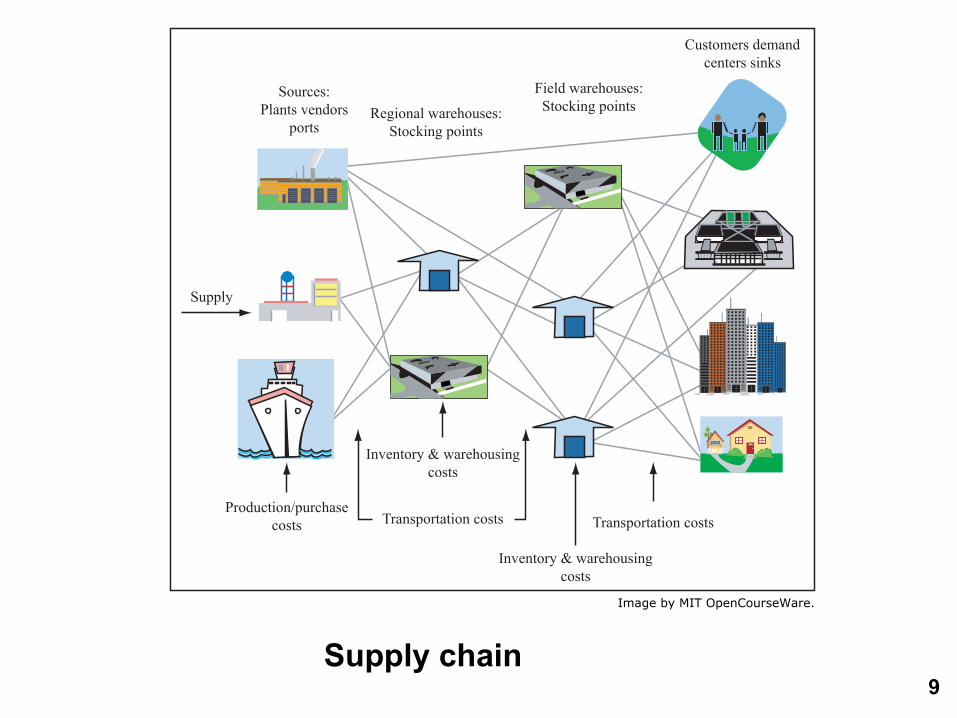
9 Supply chain

Sources:Plants vendors

portsRegional warehouses:

Stocking points

Field warehouses:Stocking points

Customers demandcenters sinks

Transportation costsTransportation costs

Inventory & warehousingcosts

Inventory & warehousingcosts

Production/purchasecosts

Supply

Image by MIT OpenCourseWare.

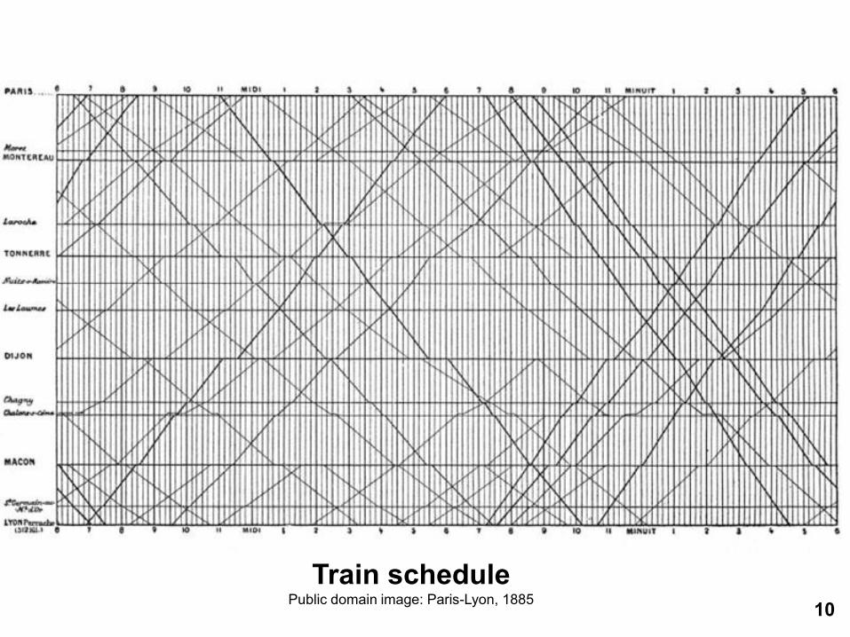
10 Train schedule

Public domain image: Paris-Lyon, 1885

11

diagram: systems dynamics Courtesy of Prof. Jim Hines. Source: 15.875 Applications of System Dynamics, Spring 2004. (MIT OpenCourseWare: Massachusetts Institute of Technology),http://ocw.mit.edu/courses/sloan-school-of-management/15-875-applications-of-system-dynamics-spring-2004 (Accessed 25 Nov, 2013).

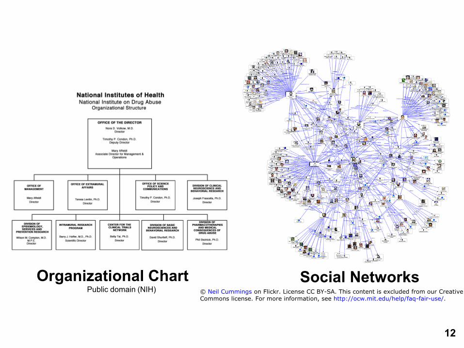
12

Organizational Chart Public domain (NIH)

Social Networks Commons license. For more information, see http://ocw.mit.edu/help/faq-fair-use/.© Neil Cummings on Flickr. License CC BY-SA. This content is excluded from our Creative

Flows in networks

Shipping from warehouses to retailers

The min cost flow problem

A remarkable theorem

13

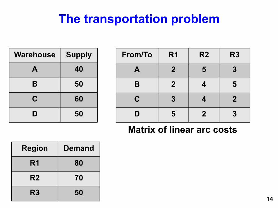
The transportation problem

14

From/To R1 R2 R3

A 2 5 3

B 2 4 5

C 3 4 2

D 5 2 3

Warehouse Supply

A 40

B 50

C 60

D 50

Region Demand

R1 80

R2 70

R3 50

Matrix of linear arc costs

The Transportation Problem

15

The transportation problem is a min cost flow problem with the following two properties:

• All arcs are directed from “supply nodes” to “demand nodes.”

• Arcs have costs, but there is no upper bound on arc flows.

1

2

3

40

50

60

50

80

70

50

2 5

A

B

C

D

3

Supply nodes

Demand nodes

2 4 5 3 4 2

5 2 3

16

An LP formulation Let xij = amount shipped from i to j assigned to task j.

xA2 xA3 xA1 RHS xB2 xB3 xB1 xC2 xC3 xC1 xD2 xD3 xD1 RHS

A 1 1 1 RHS 0 0 0 0 0 0 0 0 0 40 B 1 1 1 0 0 0 0 0 0 RHS 0 0 0 50 C 1 1 1 0 0 0 0 0 0 RHS 0 0 0 60 D 1 1 1 0 0 0 RHS 0 0 0 RHS 0 0 0 50

1 0 0 1 RHS 0 0 1 0 0 1 0 0 1 80 2 1 0 0 RHS 1 0 0 1 0 0 1 0 0 70 3 0 1 0 RHS 0 1 0 0 1 0 0 1 0 50

17

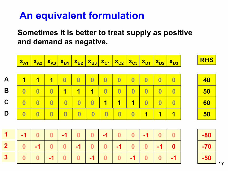
An equivalent formulation Sometimes it is better to treat supply as positive and demand as negative.

xA2 xA3 xA1 RHS xB2 xB3 xB1 xC2 xC3 xC1 xD2 xD3 xD1 RHS

A 1 1 1 RHS 0 0 0 0 0 0 0 0 0 40 B 1 1 1 0 0 0 0 0 0 RHS 0 0 0 50 C 1 1 1 0 0 0 0 0 0 RHS 0 0 0 60 D 1 1 1 0 0 0 RHS 0 0 0 RHS 0 0 0 50

1 0 0 1 RHS 0 0 1 0 0 1 0 0 1 80 2 1 0 0 RHS 1 0 0 1 0 0 1 0 0 70 3 0 1 0 RHS 0 1 0 0 1 0 0 1 0 50

1 0 0 -1 RHS 0 0 -1 0 0 -1 0 0 -1 -80 2 -1 0 0 RHS -1 0 0 -1 0 0 -1 0 0 -70 3 0 -1 0 RHS 0 -1 0 0 -1 0 0 -1 0 -50

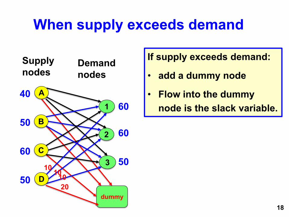
When supply exceeds demand

18

50

60

60

If supply exceeds demand:

• add a dummy node

• Flow into the dummy node is the slack variable.

dummy

1

2

3

40

50

60 50

A

B

C

Supply nodes

Demand nodes

20

10 10 10 D

19

Supply/demand constraints

xij = flow in (i, j) node supply/demands bi

We always assume that Σ bi = 0.

That is, the available supply equals the required demand. This is wlog. More on that latter.

1

2

4

3 3

7

-2

-8

Flow out of node i - Flow into node i = bi

Example: Node 4

x42 – x14 – x34 = -8

20

x14 x23 x32 x34 x42 x12 RHS

1 0 0 0 0 1 7 0 1 -1 0 -1 -1 3 0 -1 1 1 0 0 -2 -1 0 0 -1 1 0 -8

= = = =

Formulating a min cost flow problem

xij = flow in (i, j) node supply/demands bi arc costs cij arc capacities uij

( , )Minimize ij iji j A

c x

0 ≤ xij ≤ uij

for all arcs (i, j) ∈ A

1

2

4

3 3

7

-2

-8

21

An LP formulation of the min cost flow problem

1

2

4

3 xij = flow in (i, j) arc costs cij arc capacities uij node supply/demands bi

0 ≤ xij ≤ uij for all arcs (i, j) ∈ A

for j ∈ N

10

n

ii

b

The amount shipped out of a node minus the amount shipped in to the node is the supply.

22

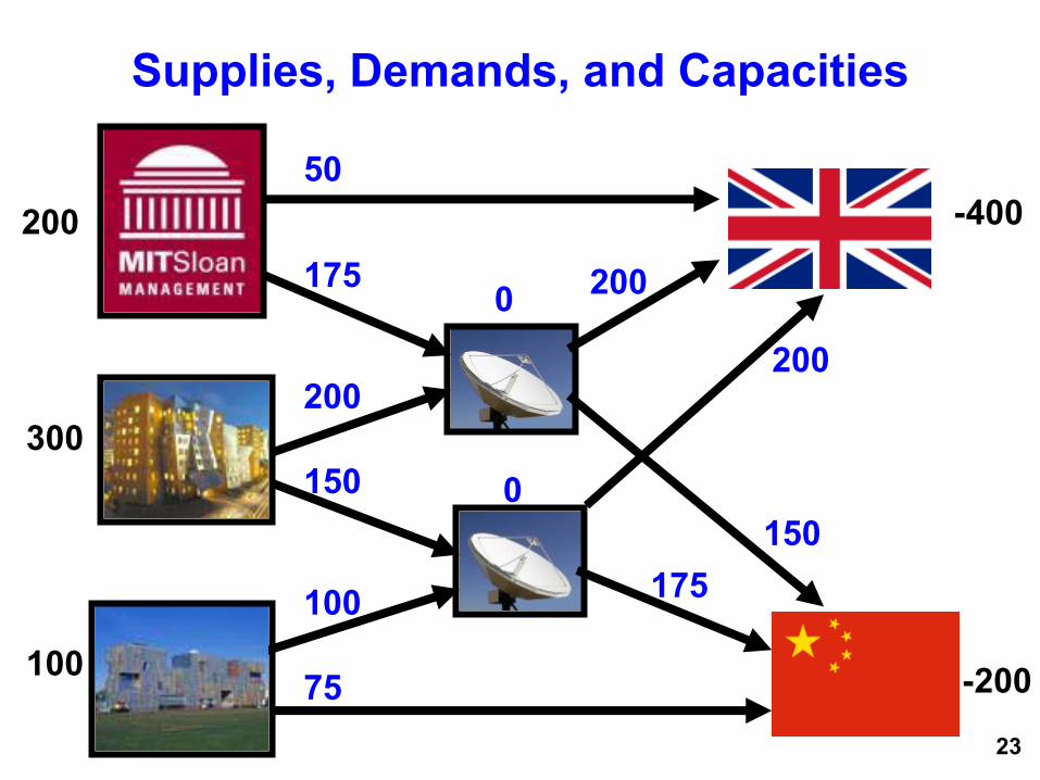
A communication problem

The year is 2013, and there is incredible demand for videos of MIT class lectures . MIT has set up three sites to handle the incredible load.

The major demand for the lectures are in London and

China. There are some direct links from each of the three MIT sites, and the lectures can be sent through two intermediate satellite dishes as well.

Each node has a supply (or a demand) indicating how

much should be shipped from (or to) the node. Each link (arc) has a unit cost of shipping flow, and a capacity on how much can be sent per second. What is the cheapest way of handling the required load?

23

Supplies, Demands, and Capacities

200

300

100

-400

-200

0

0

50

175

200

150

100

75

200

150

200

175

24

Costs per megabyte. And node labels

$ 0

$ .01

$.01

$.01

$.02

$ 0

$. 01

$. 01

$. 03

$. 04

1

2

3

4

5

6

7

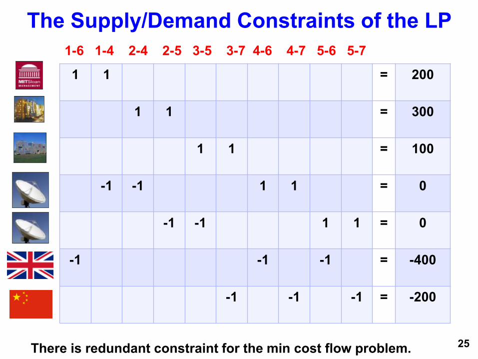
The Supply/Demand Constraints of the LP

25

1 1 = 200

1 1 = 300

1 1 = 100

-1 -1 1 1 = 0

-1 -1 1 1 = 0

-1 -1 -1 = -400

-1 -1 -1 = -200

1-6 1-4 2-4 2-5 3-5 3-7 4-6 4-7 5-6 5-7

There is redundant constraint for the min cost flow problem.

26

The Optimal Flows

200

300

100

-400

-200

0

0

50

150

175

125

25

75

200

125

150

0

✓

Which of the following is false?

27

1. If we consider all of the supply/demand constraints of a min cost flow problem, then each column has a coefficient that is 1, a coefficient that is -1, and all other coefficient are 0.

2. There is always a feasible solution for a min cost flow problem.

3. The supplies/demands sum to 0 for a min cost flow problem that is feasible.

4. At least one of the constraints of the min cost flow problem is redundant.

28

Mental Break

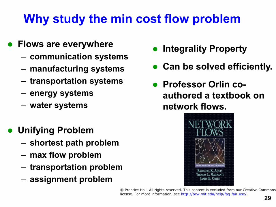
Why study the min cost flow problem

Flows are everywhere – communication systems – manufacturing systems – transportation systems – energy systems – water systems

Unifying Problem

– shortest path problem – max flow problem – transportation problem – assignment problem

29

Integrality Property

Can be solved efficiently.

Professor Orlin co-authored a textbook on network flows.

© Prentice Hall. All rights reserved. This content is excluded from our Creative Commonslicense. For more information, see http://ocw.mit.edu/help/faq-fair-use/.

30

A Remarkable Theorem. (Integrality Theorem) If the supplies, demands, and capacities of a minimum

cost flow problem are all integral, then every basic feasible solution is integer valued. Therefore, the simplex method will provide an integer optimal solution. Note: Most linear programs can have fractional solutions. x + y = 1, x – y = 0. Unique solution (.5, .5)

Reason: The coefficients in the LHS of the constraints in the tableau remain as 0, 1 or -1.

Microsoft ® Excel

✓

Which of the following is false about the integrality theorem for min cost flows?

1. It is remarkable. 2. It is in contrast to the fact that most linear programs

are not guaranteed to have integer valued bfs’s. 3. It is remarkable. 4. It can be very useful in solving integer programs. 5. It was first proved to be true by Professor Orlin.

31

More on the integrality theorem

32

Valid for LPs in which the coefficients in each column (ignoring the objective coefficients and the RHS) have at most one 1 and at most one -1, with all other elements being 0.

Does not depend on the costs. Does depend RHS being integral. Does depend on upper and lower bounds on variables being integer.

2 3 $.04

4 7 1.6

OK

Bad

Bad 6 1 u61 = 4.2

33

It is a theorem about basic feasible flows. Non-basic flows can be fractional.

1 2 2

-2

A network with arc costs. Suppose uij = 1 for all (i, j)

Suppose b(i) = 0 for all i.

1 2 0

0

Optimal Flow 1 cost = 0

1 2 1

1

Optimal Flow 2 cost = 0

1 2 .5

.5

Optimal Flow 3 cost = 0

✓

Which is not needed to guarantee that each bfs for a minimum cost flow problem has integer solutions?

34

1. Supplies/Demands are all integer valued

2. Capacities are integer valued

3. Costs are integer valued

4. All the above are needed.

Special cases of the min cost flow problem

Shortest path problem

Maximum flow problem

Assignment problem

35

36

1

2

3

4

5

3

5

1

3

3

2

1

2

3

4

5

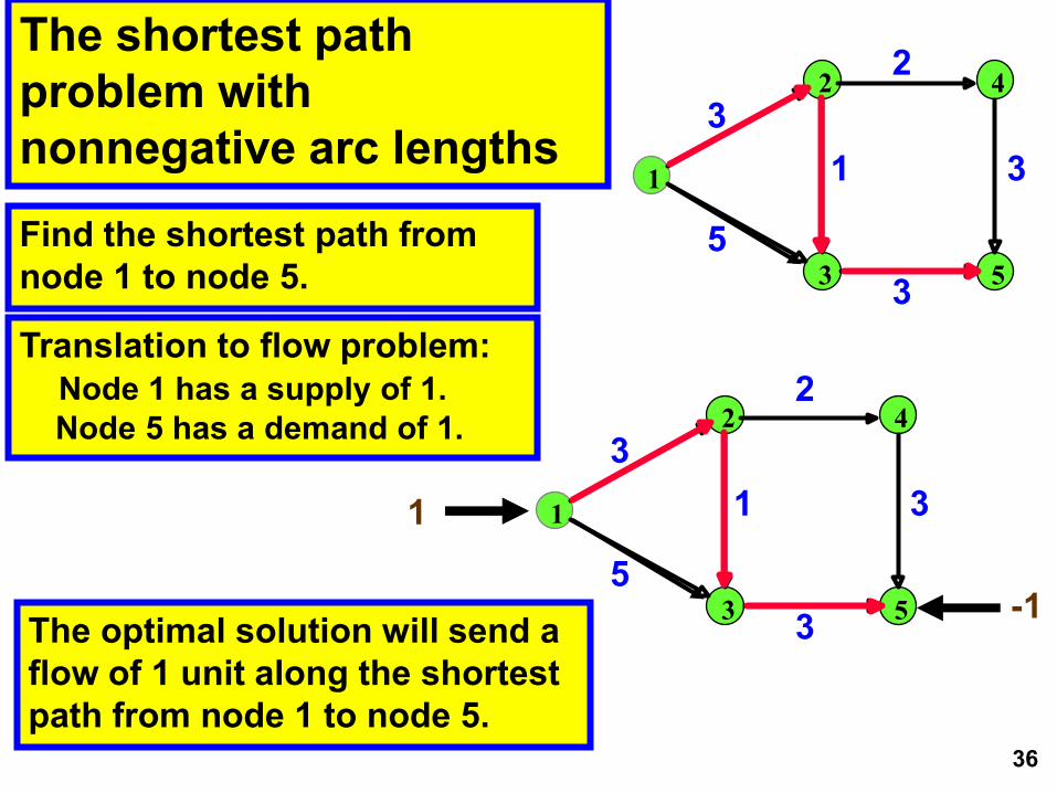
The shortest path problem with nonnegative arc lengths

3

5

1

3

2

3

Find the shortest path from node 1 to node 5.

Translation to flow problem: Node 1 has a supply of 1. Node 5 has a demand of 1.

1

-1 The optimal solution will send a flow of 1 unit along the shortest path from node 1 to node 5.

37

The Maximum Flow Problem

Directed Graph G = (N, A). – Source s – Sink t – Capacities uij on arc (i,j) – Maximize the flow out of s, subject to – Flow out of i = Flow into i, for i ≠ s or t.

A Network with arc capacities

s

1

t

2

4

1

2

3

1

The maximum flow

s

1

t

2

3

1

2

2

1

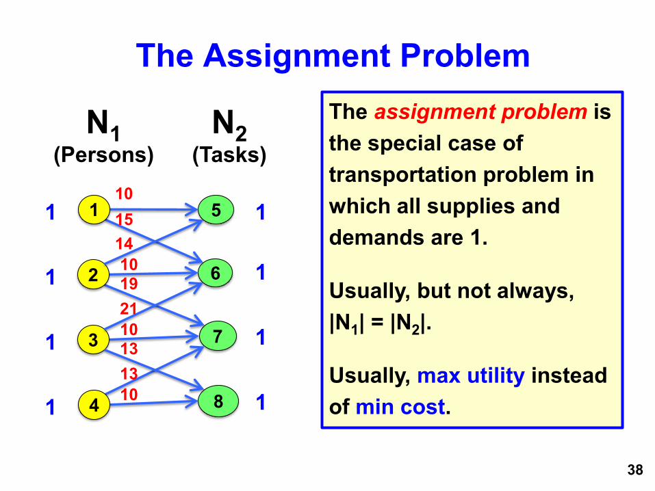
The Assignment Problem

38

5

6

7

8

1

1

1

1

1

1

1

1

10 15

10 19

10 13

10

1

2

3

4

14

21

13

The assignment problem is the special case of transportation problem in which all supplies and demands are 1.

Usually, but not always, |N1| = |N2|.

Usually, max utility instead of min cost.

N1 (Persons)

N2 (Tasks)

39

An assignment problem

Three MIT hackers have decided to make the great dome look like R2D2, in honor of the hack from 5/17/99.

Tasks. – Putting the sheets on the great dome – Ladder holder – Lookout

– Objective: find the optimal allocation of persons to

tasks.

– What is the optimal assignment of hackers to tasks.

40

10

8

9

5

10

5

9

The arc numbers are utilities.

The goal is to find an assignment with maximum total utility.

Hacker 1

Hacker 2

Hacker 3

Task 1

Task 2

Task 3

41

An LP formulation Let xij = proportion of time that hacker i is

assigned to task j.

x12 x21 x22 x23 x32 x33 x11 RHS

1 0 0 0 0 0 1 1 0 1 1 1 0 0 0 1 0 0 0 0 1 1 0 1

0 1 0 0 0 0 1 1 1 0 1 0 1 0 0 1 0 0 0 1 0 1 0 1

Hacker 1 Hacker 2 Hacker 3

Task 1 Task 2 Task 3

42

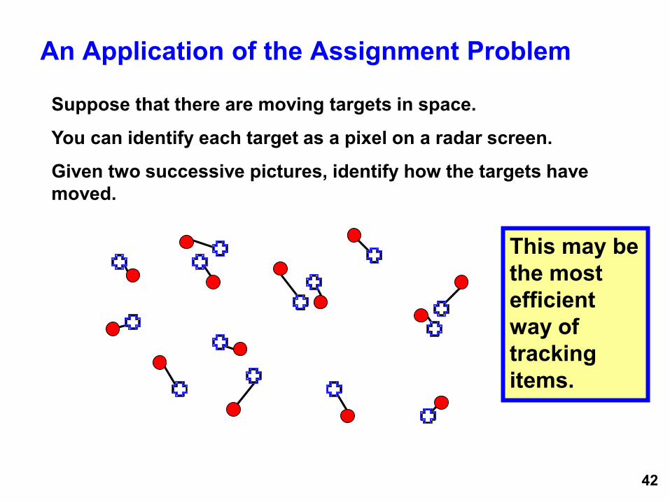
An Application of the Assignment Problem

Suppose that there are moving targets in space.

You can identify each target as a pixel on a radar screen.

Given two successive pictures, identify how the targets have moved.

This may be the most efficient way of tracking items.

43

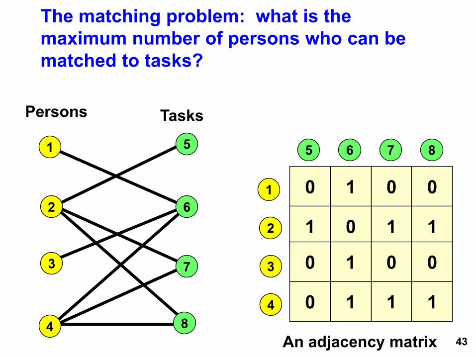
The matching problem: what is the maximum number of persons who can be matched to tasks?

0 1 0 0

1 0 1 1

0 1 0 0

0 1 1 1

An adjacency matrix

4

1

3

2

8 6 5 7

4

1

3

2

8

6

5

7

Persons Tasks

44

The matching problem

4

1

3

2

8

6

5

7

0 1 0 0

1 0 1 1

0 1 0 0

0 1 1 1

An adjacency matrix

4

1

3

2

8 6 5 7

A matching of cardinality three corresponds to three 1’s of the adjacency matrix, no two of which are in the same row or column.

0 1 0 0

1 0 1 1

0 1 0 0

0 1 1 1

An adjacency matrix

4

1

3

2

8 6 5 7

45

Independent 1’s and line covers

Max-Matching Min-Cover The minimum number of lines to cover all of the 1’s of a matrix is equal to the max number of 1’s no two of which are on a line.

Matrix rounding

46

.3 0 .4 .7

.5 .7 0 1.2

.2 .6 .2 1.0 1.0 1.3 .6

row sums

col sums

x11 x12 x13 x21 x22 x23 x31 x32 x33 col

sums

|x11 – .3| < 1

|x21 – .5| < 1

|x31 – .2 | < 1

|x11 + x21 + x31 – 1.0 | < 1

Round coefficients of the matrix up or down so that the row sums and columns sum are also rounded.

Application to matrix rounding

47

0 ≤ x11 ≤ 1 x12 = 0 0 ≤ x13 ≤ 1 0 or 1 0 ≤ x21 ≤ 1 0 ≤ x22 ≤ 1 x23 = 0 1 or 2 0 ≤ x31 ≤ 1 0 ≤ x32 ≤ 1 0 ≤ x33 ≤ 1 1

1 1 or 2 0 or 1

row sums

col sums

x11 + x21 + x31 = 1

Round coefficients of the matrix up or down so that the row sums and columns sum are also rounded.

48

An LP formulation Let xij = value in row i and column j. Let r1, r2, c2 and c3 be slack variables.

x12 x13 x11 RHS x22 x23 x21 x32 x33 x31 r2 c2 r1 RHS c3

1 1 1 RHS 0 0 0 0 0 0 0 0 1 1 0

1 1 1 0 0 0 1 0 0 RHS 0 0 0 2 0

1 1 1 0 0 0 0 0 0 RHS 0 0 0 1 0

0 0 1 RHS 0 0 1 0 0 1 0 0 0 1 0

1 0 0 RHS 1 0 0 1 0 0 0 1 0 2 0

0 1 0 RHS 0 1 0 0 1 0 0 0 0 1 1

49

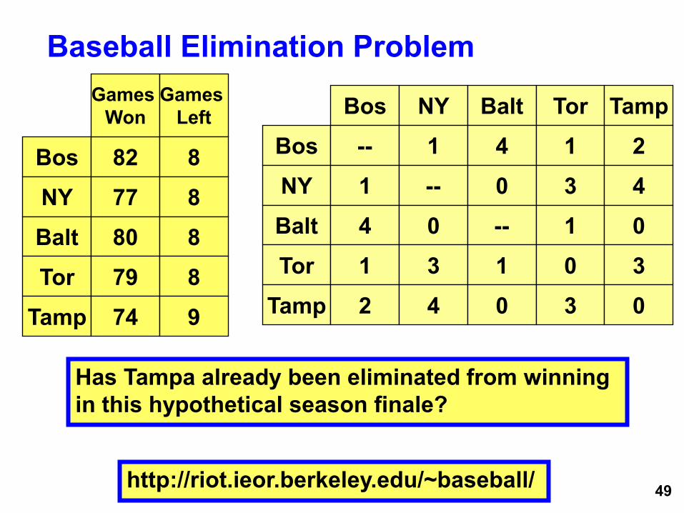
Baseball Elimination Problem

Has Tampa already been eliminated from winning in this hypothetical season finale?

http://riot.ieor.berkeley.edu/~baseball/

Bos

NY

Balt

Tor

82

77

80

79

Games Won

Games Left

8

8

8

8

Tamp 74 9

Bos NY Balt Tor

Bos

NY

Balt

Tor

-- 1 4 1

1 -- 0 3

4 0 -- 1

1 3 1 0

Tamp 2 4 0 3

Tamp

2

4

0

3

0

Is there a way for Tampa to be tied for the lead (or winning) at the end of the season?

50

Assume that Tampa wins all of their games.

• If they can’t lead the division after winning all of their games, they certainly can’t lead if they lose one or more games.

Question: is it possible to assign wins and losses to all remaining games so that Tampa ends up in first place?

51

Bos NY Balt Tor

Bos

NY

Balt

Tor

-- 1 7 1

1 -- 0 3

7 0 -- 1

1 3 1 0

Tamp 2 4 0 3

Tamp

2

4

0

3

0

Bos

NY

Balt

Tor

82

77

80

79

Games Won

Games Left

11

8

8

8

Tamp 74 9

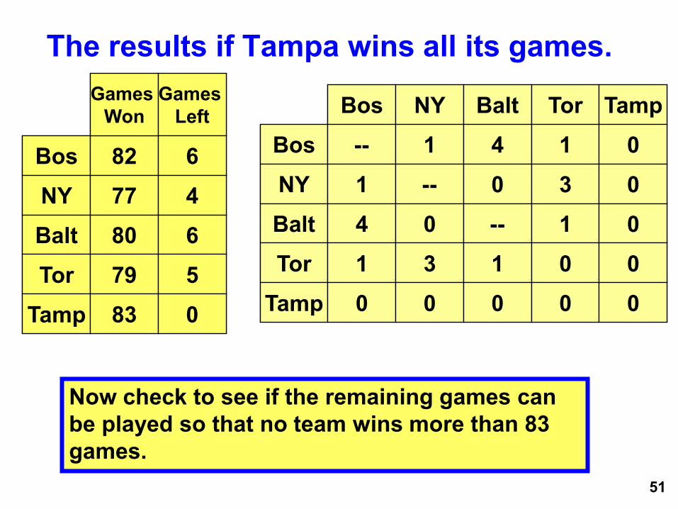
The results if Tampa wins all its games.

Now check to see if the remaining games can be played so that no team wins more than 83 games.

Bos

NY

Balt

Tor

82

77

80

79

Games Won

Games Left

6

4

6

5

Tamp 83 0

Bos NY Balt Tor

Bos

NY

Balt

Tor

-- 1 4 1

1 -- 0 3

4 0 -- 1

1 3 1 0

Tamp 0 0 0 0

Tamp

0

0

0

0

0

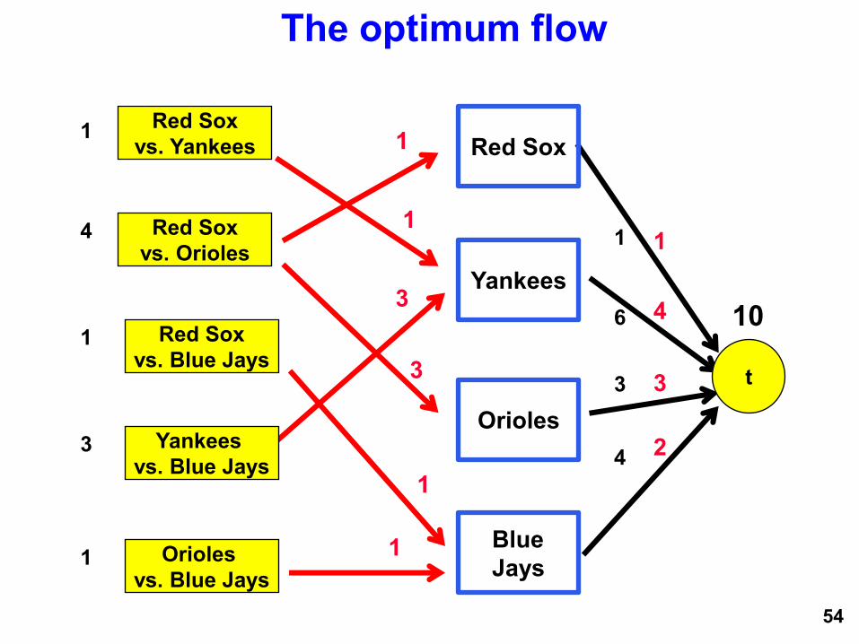
Constraints

Upper bound on the number of games won by each team (except Tampa).

Each game is won by one of the two teams playing the game.

The flow on an arc is the number of games won.

52

53

10

1

6

3

4

t

Red Sox vs. Orioles

4

Red Sox vs. Blue Jays

1

Yankees vs. Blue Jays

3

Orioles vs. Blue Jays

1

1 Red Sox vs. Yankees

Flow on (i,j) is interpreted as games won.

Red Sox

Yankees

Orioles

Blue Jays

54

10

1

6

3

4

t

Red Sox vs. Orioles

4

Red Sox vs. Blue Jays

1

Yankees vs. Blue Jays

3

Orioles vs. Blue Jays

1

1 Red Sox vs. Yankees

The optimum flow

1

3

1

3

1

1

1

4

3

2

Red Sox

Yankees

Orioles

Blue Jays

55

Some Information on the Min Cost Flow Problem

Reference text: Network Flows: Theory, Algorithms, and Applications by Ahuja, Magnanti, and Orlin [1993]

15.082J/6.885J: Network Optimization

Polynomial time simplex algorithm (Orlin [1997])

Basic feasible solutions of a minimum cost flow problem are integer valued (assuming that the data is integer valued)

Very efficient solution techniques in practice

MIT OpenCourseWarehttp://ocw.mit.edu

15.053 Optimization Methods in Management ScienceSpring 2013

For information about citing these materials or our Terms of Use, visit: http://ocw.mit.edu/terms.