The Mindanao and Halmahera eddies –twin eddies induced by nonlinearities

WILTON Z. ARRUDA1 AND DORON NOF

2

Department of Oceanography,

The Florida State University, Tallahassee, Florida

Submitted to Journal of Physical Oceanography

Revised, April 2003

Corresponding author address: Prof. Doron Nof, Department of Oceanography 4320,Florida State University, Tallahassee, FL 32306-4320, USAEmail: nof@ocean.fsu.edu

1Permanent affiliation: Departamento de Métodos Matemáticos, Universidade Federal do Rio

de Janeiro, BRAZIL2Additional affiliation: Geophysical Fluid Dynamics Institute, The Florida State University,

Tallahassee, Florida

Abstract

It is shown analytically that a nonlinear collision of northward and southward flowing

western boundary currents (WBC) on a β-plane produces both an anticyclonic and a cyclonic

eddy. (On an f-plane no eddies are established; similarly, no eddies are established in the linear

limit.) The length scales of both the anticyclonic and cyclonic eddies are larger than most eddies

in the ocean. Furthermore, the anticyclone scale is larger than the cyclone length scale due to the

higher upstream momentum flux. A reduced gravity numerical model is used to validate these

analytical results. The balance of forces and the eddy size estimates (derived form the numerical

simulations) agree with the analytical results.

Based on the above collision problem, it is argued that the Halmahara and Mindanao

eddies are required to balance the nonlinear momentum fluxes of their colliding parent currents,

the southward flowing Mindanao Current (MC) and the northward flowing South Equatorial

Current (SEC). Assuming that the interior is in Sverdrup balance, it is further argued that neither

of the eddies would have been present had the Indonesian Throughflow not been active.

1

1. Introduction

The western equatorial Pacific plays a key role in the establishment of El Niño/Southern

Oscillation (ENSO) events and may also be an important part of the so-called “great conveyor

belt”(e.g., Gordon 1986) because of the Pacific-to-Indian throughflow (ITF). The eddies and

low-latitude western boundary currents (WBC) addressed here (Fig. 1) are important aspects of

these processes.

The equatorward-flowing WBCs provide the closure to two symmetrical gyres relative to

the equator (Kessler and Taft 1987). One gyre is entirely in the Northern Hemisphere whereas

the other (which is mostly in the Southern Hemisphere) crosses the equator. The North

Equatorial Counter-Current (NECC) forms the boundary between these two gyres at about 5˚N.

North of the NECC the westward-flowing North Equatorial Current (NEC) bifurcates (Toole et

al. 1990) into the northward-flowing Kuroshio and the southward-flowing Mindanao Current

(MC). A similar situation takes place in the Southern Hemisphere where the westward-flowing

South Equatorial Current (SEC) bifurcates (around 15˚S) into a branch flowing northwestward

and a branch flowing southward. Along the New Guinea coast the northwestward-flowing

branch of the SEC is usually recognized as a subsurface current, the New Guinea Coastal Under-

Current (NGCUC), and a surface current, the New Guinea Coastal Current (NGCC). The NGCC

retroflects to the east of the Halmahera Island and joins the retroflected flow of the MC to flow

eastward as the NECC.

There are two semi-permanent eddies in the retroflection area of the MC and SEC

(Fig. 1). The first, the Mindanao eddy (ME), is situated north of the NECC (near 7˚N, 128˚E)

and has cyclonic circulation, whereas the second, the Halmahera eddy (HE), which is situated

south of the NECC (near 4˚N, 130˚E) has anticyclonic circulation (Wyrtki 1961). The reason for

the existence of the eddies is not obvious. One would intuitively expect that such eddies are

established by friction which enables the turning fluid to drag some interior fluid along with it as

it turns. Another possibility would be that the eddies result from instability of the eastward

flowing NECC and the westward propagation of such instabilities. We shall show in this article

2

that neither of the two ideas is correct. We shall demonstrate that both friction and instability do

not play any role in the establishment of the eddies. Rather, it is nonlinearity and β which are

responsible for the establishment of the eddies. In what follows we shall briefly describe the two

colliding boundary currents (MC and SEC) and the two eddies.

a. Observational background

1. The Mindanao Current (MC). The MC extends to a depth of 600 m and a distance

of 100 km offshore (Wyrtki 1961, Masuzawa 1968). Wyrtki (1956, 1961) first estimated a

baroclinic transport ranging from 8 to 12 Sv (1 Sv =106 m2s-1) in the upper 200 m and 25 Sv in

the upper 1000 m. Different transport estimates were later made by Masuzawa (1969) who gave

a transport from 13 to 29 Sv relative to 600 dbar, Kendall (1969) who argued that the MC carries

14 Sv, Cannon (1970) who estimated a geostrophic transport of 18 to 31 Sv relative to 1000

dbar, Toole et al.(1988) who gave a transport of 17-18 Sv for waters warmer than 12˚C, and

Lukas et al.(1991) who calculated a transport from 13 Sv to 33 Sv between 10˚N and 5.5˚N.

Regardless of the values that one chooses, the velocities are relatively high [O(1)m s-1] and the

width is fairly narrow (150 km). These give a fairly high Rossby number (~ 0.5 taking into

account that the maximum speed is at that jet's center) suggesting that the current is nonlinear.

2. The Mindanao eddy (ME). Takahashi (1959) first noted the existence of ”a cold

region of distorted elliptic form” east of the MC and related this feature to the cyclonic

circulation inferred from dynamic topography. This closed circulation is named the “Mindanao

eddy” following the work of Wyrtki (1961) who noted that the ME is a quasi-permanent eddy

associated with the turning of the NEC waters at the coast of the Philippines and its subsequent

flow to the east as part of the NECC. The existence of the eddy was later verified by Lukas et al.

(1991) who reported that drifters launched in the ME described closed loops with diameters of

about 250 km and by Qu et al. (1999) who identified the ME as a depression (of less than 130 m)

3

in the 24.5 σθ isopycnal surface centered at 7˚N, 129˚E.

3. The South Equatorial Current and the New Guinea Coastal Current. As mentioned,

the westward-flowing SEC bifurcates near 15˚S. The equatorward branch of the Great Barrier

Reef Undercurrent (Church and Boland 1983) later flows into the NGCUC. A shallow current

(NGCC) overlying the NGCUC was first observed by Masuzawa (1968). Cantos-Figuerola and

Taft (1983) found an NGCC transport of 11 Sv whereas Wyrtki and Kilonsky (1984) estimated a

total transport (NGCC plus NGCUC) of about 40 Sv. Gouriou and Toole (1993) found a total

transport of 24.8 Sv from direct measurements, 37.7 Sv from geostrophy relative to 600 dbar,

and 41.7 Sv from geostrophy relative to 1000 dbar. Like the MC, the NGCC is fairly nonlinear

with a Rossby number of approximately 0.4.

4. The Halmahera eddy (HE). As with the ME, the HE appears in the dynamics

topography maps of Takahashi (1959) and was named after the work of Wyrtki (1961). It is well

developed only during the northern summer monsoon, when the South Pacific water from the

NGCC re-curves into the NECC. Within the HE, Lukas’ et al.(1991) drifters executed closed

loops of about 300 km diameter and velocity of about 50 cm s-1. Using shipboard ADCP,

Kashino et al.(1999) identified the center of the Halmahera eddy to be east of 130˚E and 4˚N.

They also identified a horizontal scale of about 500 km (at 50 m).

b. Modeling and theoretical background

It is sufficient to point out here that there are no explanations for the establishment of the

eddies primarily because the earlier theories are linear (i.e., quasigeostrophic) which, as we shall

see, filters out the eddy generation mechanism (Cessi 1990, 1991) or f-plane theories (Lebedev

and Nof 1996, 1997) which also filters out the eddies.

Before proceeding, it is appropriate to point out that the Indonesian Throughflow (ITF) is

4

critical to the collision of the MC and the NGCC and, therefore, to the establishment of the

eddies. Arruda (2002) showed that, without any net meridional flow a few degrees north of the

equator (i.e., no ITF), there would be no WBC transport and, hence, no collision and no eddies.

This is consistent with the picture described in Nof (1998) (see his Fig. 2) where, due to the

vanishing wind stress curl a few degrees north of the equator (implying zero Sverdrup transport

there) and the absence of deep water formation in the northern Pacific, there can be no WBC a

few degrees north of the equator unless the basin has “holes.” Namely, with Sverdrup dynamics

and zero wind stress curl north of the equator, a no-ITF scenario must involve no net WBC

transport (i.e., no collision) because, in a closed basin, the WBC transport is equal and opposite

to the interior transport (zero in our case).

c. Present work

As mentioned, our goal is to examine the nonlinear collision of opposing WBCs on a β-

plane. We shall see that it is the nonlinear curving of these retroflecting currents and β which are

responsible for the generation of the eddies. Since our problem involves nonlinearity, a “head-

on” approach is not useful and we shall look at the problem in terms of integrated momentum

flux balances which circumvent the need to find a solution valid in the entire field. Before

attacking the full collision problem, it is useful to first examine the behavior of currents in a

concave solid corner formed by a solid boundary. We shall do so by using the momentum flux

approach (see e.g., Lebedev and Nof 1996, 1997) and begin by examining a northward flowing

current.

This paper is organized as follows. After presenting the method of analysis in Section 2,

we address the problem of a WBC in a concave solid corner in Section 3. In Section 4 we focus

on the collision problem, and in Section 5 we apply the results of the previous sections to the

equatorial western Pacific and suggest the physical mechanism responsible for the existence of

the ME and HE. The conclusions are given in section 6.

5

3. Flow in a concave solid corner

a. Analytical considerations

1. Formulation. As the WBC (Fig. 2) flows northward, it encounters a zonal wall that

forces it to change direction and flow eastward. Assuming a steady state and integrating (after

multiplying by h) the steady and inviscid nonlinear y-momentum equation over the fixed region

S bounded by the dashed line ABCDA (shown in the upper left panel in Fig. 2), we get,

∂∂ +

∂( )∂

∂∂

∂∂ −

∫∫ ∫∫∫∫ ( ) – – ( )huv

xhvy

dxdy fy

dxdy yy

dxdyS SS

2

0

ψ β ψ βψ

+∂

∂ =∫∫g hy

dxdyS

' ( ).

20

2

(3)

Application of Green's theorem gives,

huvdy hvg h

f y dx dxdyS S S∂ ∂∫ ∫ ∫∫+ +

+ =– '

– ( ) ,22

020β ψ β ψ (4)

where ∂S is the boundary of S and g' is the “reduced gravity,” g∆ρ/ρ.

Next, we take ψ = 0 along the wall and note that at least one of the velocity components

vanishes on every portion of the boundary ∂S. It then follows from (4) that,

hvg h

f y dxg h

dx dxdyA

B

C

D

S

22

0

2

2 20+ +

=∫ ∫ ∫∫'

– ( ) –'

– .β ψ β ψ (5)

Assuming now (and later verifying with our numerics) that, away from the corner, the flow is

geostrophic in the cross-current direction, we get [after multiplying the geostrophic relation (f0

+βy)v = g'∂h/∂x by h and integration in x],

6

( ) ( , ) .f y h h ys02 20+ = −[ ]β ψ (6)

Combining (5) and (6) we get our desired expression,

hv dxg

h y h x dx dxdyL

s

L

S

2

0

2 2

020 0 0

2

∫ ∫ ∫∫+ −( ) − =

WBCmom.flux Pressure term term1 24 34 1 244444 344444 1 24 34

'( , ) ( , ) ,β ψ

β

(7)

where L is the boundary current width and L2 is the zonal extent of our region S. It is straight-

forward to show that, for southward-flowing WBC, the equivalent momentum balance in the

region S (bounded by ABCD) is very similar.

2. The f-plane limit. Although β is important for the establishment of the WBC in the

first place, once a WBC is established, the role of β is frequently minor particularly if the process

in question is of the Rossby radius scale. For this reason, it makes sense to first examine the

behavior of a boundary current on an f-plane.

On an f-plane the pressure force should balance the WBC momentum flux if a steady

state is to be established. To see this, note that, as we approach the corner, the velocity along the

wall gradually decreases to zero (see Kundu 1990, Chapter 4). Since the wall is a streamline, the

Bernoulli function [B = g'h +(u2 + v2)/2] implies that the upper layer thickness increases to a

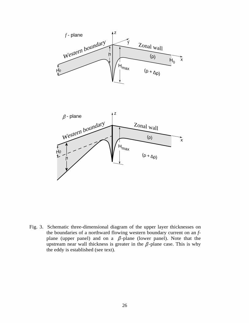
maximum at the corner (Fig. 3, upper panel). Consequently, the pressure force in (7) points in

the opposite direction to that of the WBC momentum force and a balance without an eddy

appears to be possible. Numerical simulations will later verify this outcome. Note that, in the

case of no zonal wall (i.e., the WBC separates due to a vanishing upper layer thickness), the

pressure term vanishes (since h = 0 on the western boundary and on the outcropping streamline).

As a result, the WBC momentum flux is unbalanced and the f-plane system cannot reach a

steady state (see Arruda et al. 2003).

3. The no eddy on a β-plane scenario. Here, we temporarily assume that no eddy is

associated with the turning boundary current on a β-plane and show that this hypothetical

7

scenario is impossible. Note that the geostrophic transport relationship [T = g'(H2 – hw2 )/2f,

where H and hw are the thicknesses off and on the wall] implies that on a β-plane the near-wall

thickness of a northward-flowing WBC decreases as we proceed downstream along the western

boundary (Fig. 3, lower panel). This implies that there is an additional pressure force (resulting

from the decreasing near-wall thickness due to β) pointing in the same sense as the upstream

momentum flux. Hence, the wall pressure cannot balance the net (upstream) northward force.

Taking the zonal extent of S to be O(Rd) we see that, in the absence of an eddy, the β-term in (7)

is negligible compared to the WBC momentum flux so that it cannot balance the WBC

momentum flux either. The no-eddy scenario is, therefore, impossible. In what follows, we first

present numerical simulations and then present our analytical solution.

b. Numerical simulation for a flow in a concave solid corner

We use a reduced gravity version of the isopycnic model developed by Bleck and Boudra

(1981, 1986) and later improved by Bleck and Smith (1990). The equations of motion are the

two momentum equations,

∂∂ +

∂∂ +

∂∂ + = ′

∂∂ + ∇⋅ ∇

ut

uux

vuy

f y v ghx h

h u– ( ) – ( )0 β ν

∂∂ +

∂∂ +

∂∂ + = ′

∂∂ + ∇⋅ ∇

ut

uvx

vvy

f y u ghy h

h v– ( ) – ( ) ,0 β ν

and the continuity equation

∂∂ +

∂∂ +

∂∂ =

ht

hux

hvy

( ) ( ),0

where ν is the frictional coefficient.

The model uses the Arakawa (1966) C-grid where the u-velocity points are shifted one-

8

half gridstep to the left from h points, the v-velocity points are shifted one-half gridstep down

from the h points, and vorticity points are shifted one-half gridstep down from the u-velocity

points. On open boundaries the Orlanski (1976) second-order radiation boundary condition was

implemented. The list of experiments is given in Table 1. The walls were slippery and the

vorticity was taken to be zero near them.

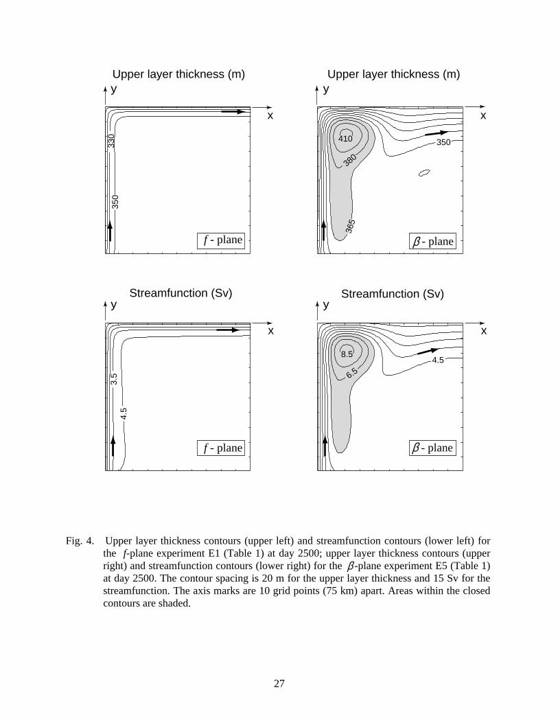
1. Northward flowing WBC in a concave corner. Fig. 4 shows the upper layer

thickness and streamfunction for the f-plane experiment E1 and the β-plane experiment E5

(Table 1) at day 2500, and Fig. 5 shows the upper layer thickness along the western boundary

and along the zonal wall. We see that, as mentioned, on an f-plane the upper layer thickness

increases to a maximum near the corner, producing a southward pressure force. For the f-plane

experiment E1 the downstream upper layer thickness along the zonal wall is 270.7 m which is

very close to our specified value of 270.3 for H0. Fig. 6 shows that the pressure force points

southward and balances the northward momentum flux of the WBC [indicating that the inviscid

balance is attained]. We also see that, as mentioned, in this f-plane case, no eddy is necessary to

achieve the momentum balance.

When β is introduced (Fig. 4), an anticyclonic eddy (attached to the curving flow) is

generated. As seen in Fig. 5, in this case, the net pressure force points northward since the upper

layer thickness along the western boundary is larger than its average value on the zonal wall

(270.2m). In addition, note that the thickening of the upper layer at the corner is compensated by

the eddy so that the average value of the upper layer thickness on the zonal wall is 270.2 m,

which is practically indistinguishable from the initial value for H0 (270.3 m). This numerical

observation will be used shortly in our detailed derivations. Figure 6 shows that the combination

of β and the pressure terms is a southward force which balances the northward momentum force

of the WBC. With the aid of (7) and a scale analysis that we shall perform later, we shall show

that the eddy is the main contributor to the combined β and pressure terms. The eddy’s β-force is

due to the particles circulation within the anticyclonic eddy which causes a greater Coriolis force

9

on the northern portion of the eddy than on the southern.

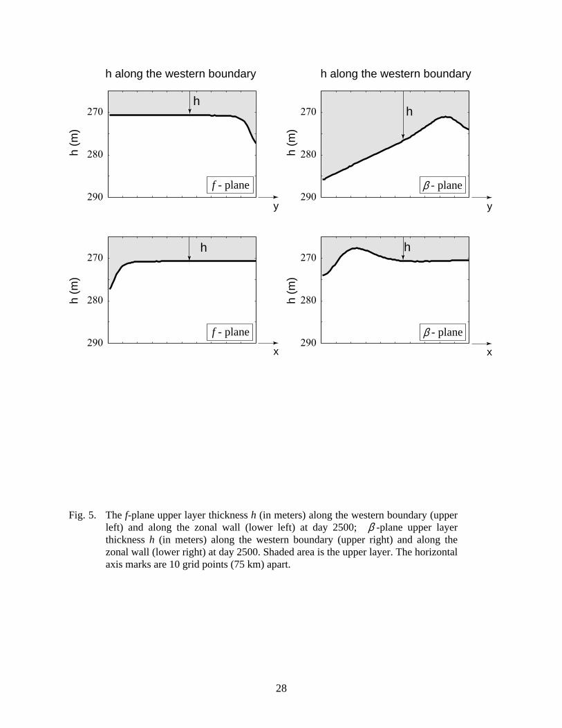
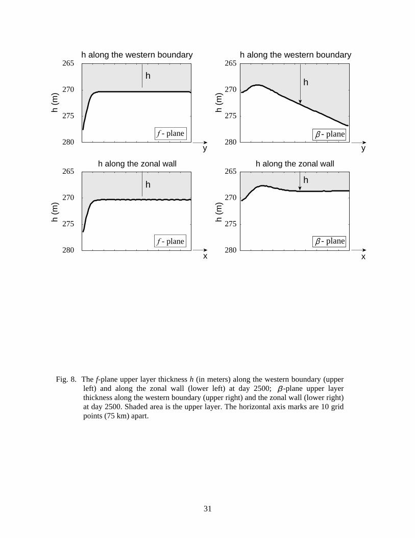
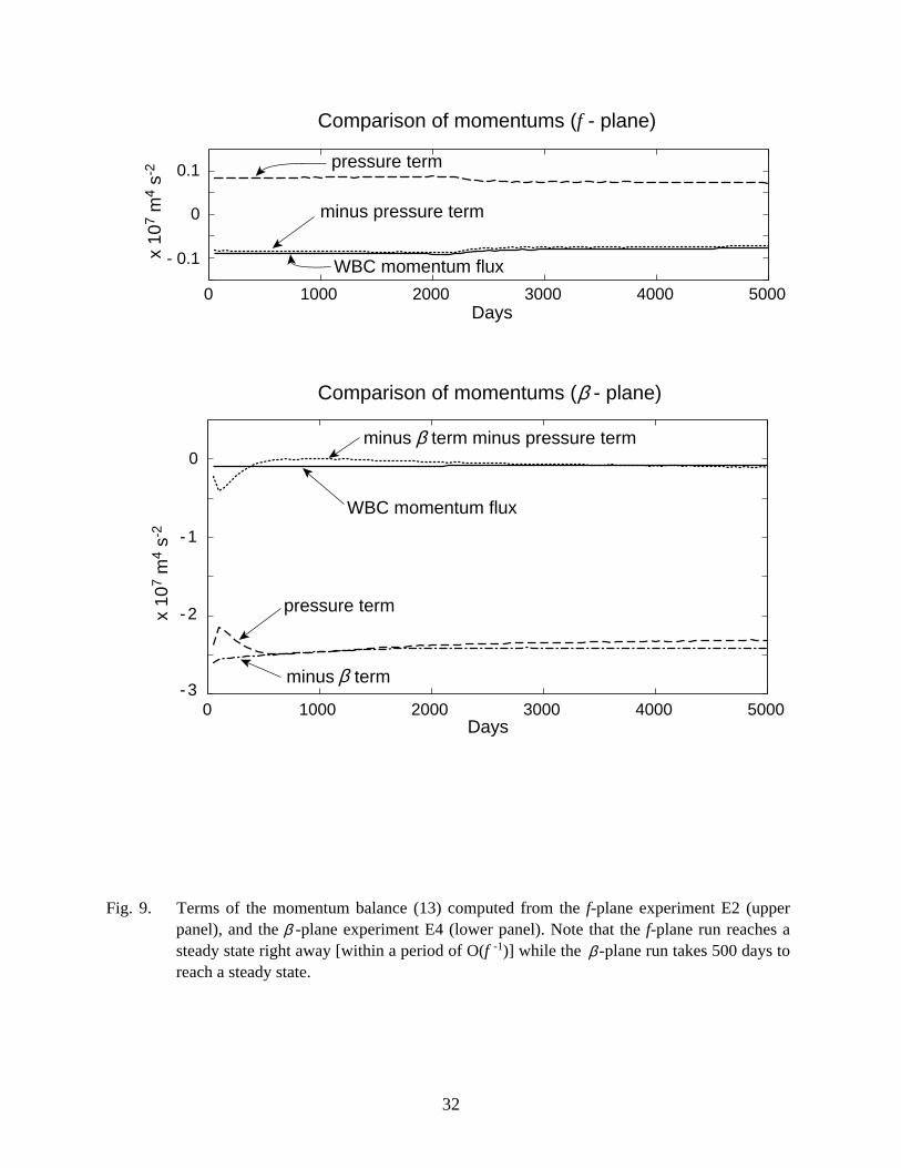
2. Southward flowing WBC in a corner. Fig. 7 shows contour plots of the upper layer

thickness and streamfunction at day 2500 for the f-plane experiment (E2) and the β-plane

experiment (E6). Similarly, Fig. 8 displays the upper layer thickness along the western boundary

and along the zonal wall at the same day. In the f-plane situation, the upper layer thickness

increases to a maximum in the corner, producing a northward pressure force which, according to

Fig. 9, balances the southward momentum force of the WBC. This indicates that the inviscid

balance is attained.

When β is introduced (Fig. 7), a cyclonic eddy is formed. Also, as seen in Fig. 8, the

pressure force points southward since the upper layer thickness along the western boundary is

larger than its average value on the zonal wall (268.6 m). The average value of the upper layer

thickness along the zonal wall is 268.6 m which coincides with its average value at the last 50

grid points, showing that the thickening at the corner (associated with the Bernoulli function

conservation) is compensated by the shallowness produced by the eddy. Again, this will shortly

be used in our derivations. As seen in Fig. 9, the combination of the β and the pressure terms is a

northward force which balances the southward momentum force of the WBC.

c. Estimates of the eddy radius

We shall now use both the analytical considerations given in (a) and the numerical

simulation given in (b) to derive an estimate for the eddy radii. An alternative form of the

momentum balance relation for northward-flowing WBC in a concave solid corner (5) can be

derived by noting that, at x → ∞ , the zonal flow is geostrophic in the y direction so that (5) can

be written as,

hv dxg

H h x dx dxdyL L

S

2

002 2

0

2

20 0+ ( ) =∫ ∫ ∫∫ ∞

'– ( , ) – ( – ) ( )β ψ ψ northward WBC (8a)

10

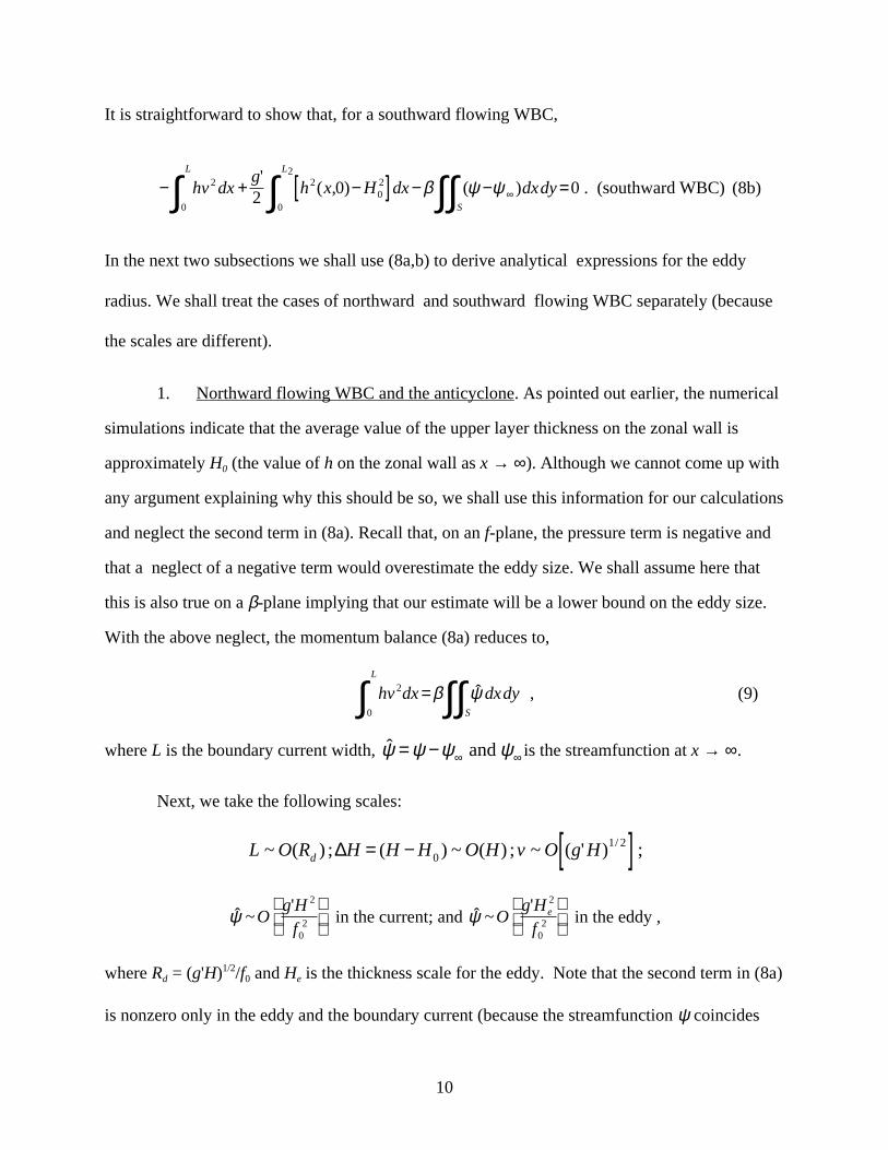
It is straightforward to show that, for a southward flowing WBC,

− + −[ ] − − =∫ ∫∫∫ ∞hv dxg

h x H dx dxdyL

S

L2

0

202

0

2

20 0

'( , ) ( ) . ( )β ψ ψ southward WBC (8b)

In the next two subsections we shall use (8a,b) to derive analytical expressions for the eddy

radius. We shall treat the cases of northward and southward flowing WBC separately (because

the scales are different).

1. Northward flowing WBC and the anticyclone. As pointed out earlier, the numerical

simulations indicate that the average value of the upper layer thickness on the zonal wall is

approximately H0 (the value of h on the zonal wall as x → ∞). Although we cannot come up with

any argument explaining why this should be so, we shall use this information for our calculations

and neglect the second term in (8a). Recall that, on an f-plane, the pressure term is negative and

that a neglect of a negative term would overestimate the eddy size. We shall assume here that

this is also true on a β-plane implying that our estimate will be a lower bound on the eddy size.

With the above neglect, the momentum balance (8a) reduces to,

hv dx dxdyS

L2

0

= ∫∫∫ β ψ , (9)

where L is the boundary current width, ψ ψ ψ ψ= − ∞ ∞and is the streamfunction at x → ∞.

Next, we take the following scales:

L O R H H H O H v O g Hd~ ( ) ; ( ) ~ ( ) ; ~ ( ' ) ;/∆ = − [ ]01 2

ˆ ~'ψ O

g Hf

2

02

in the current; and ˆ ~'ψ O

g Hf

e2

02

in the eddy ,

where Rd = (g'H)1/2/f0 and He is the thickness scale for the eddy. Note that the second term in (8a)

is nonzero only in the eddy and the boundary current (because the streamfunction ψ coincides

11

with ψ∞ in the interior). Following Nof and Pichevin (1999) we now take Rde = Rd/ε1/6 where ε ≡

βRd/f0 and obtain the leading order balance,

h dx dx dyL

e e eSe

( ) ( )

( )

( ) * *( ) * ,0 0 2

0

0

0v∫ ∫∫= ψ (10)

where h(0)

, v(0)

, ψe( )0 , and L

(0) are the zeroth-order approximations of the respective dependent

variables.

Next, we take the flow to have zero potential vorticity and find that the solutions are

straightforward despite the nonlinearity. Note that, with this assumption, the interior of the basin

is motionless (with thickness H) and the velocity is zero long the bounding streamline of the

current offshore (see e.g., Anderson and Moore 1979). As we shall see later, in this limit, the

obtained estimate is a lower bound on the eddy radius. The leading order velocity and thickness

for a zero-potential vorticity northward flowing boundary current are,

v =− ≤

>

f L x x L

x L0

0

( ) ,(11)

h Hf L x

gx L

H x L= −

−≤

>

02 2

2( )

',

, ,(12)

where L = 21/2 Rde, where Rde = [g'(H – H0)]1/2

/f0. Since the eddy’s upper layer thickness scale is

He = H(Rde/Rd)2 = ε-1/3H, we can take he = 0 along the eddy’s boundary and find that, for the zero

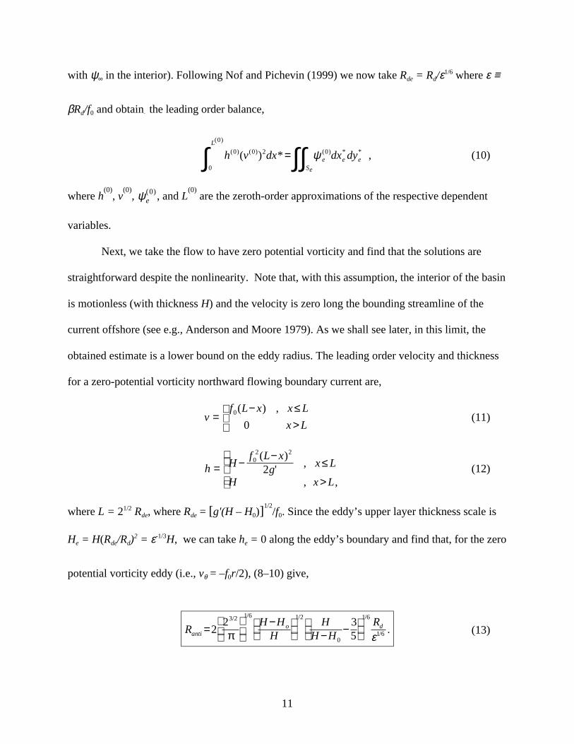
potential vorticity eddy (i.e., vθ = –f0r/2), (8–10) give,

RH H

HH

H HR

antio d= π

−

− −

2

2 35

3 2 1 6 1 2

0

1 6

1 6

/ / / /

/ .ε (13)

12

This relation is a lower bound, because the zero potential vorticity eddy has the strongest

nonlinearity (due to the highest steepness) and, consequently, it also has the smallest radius.

To validate (13) we determine analytically the numerical eddy radius using the

parameters of the numerical experiment E5 (Table 1), getting ε1/6 = 0.42 and R = 2.84 Rd. Taking

the streamline corresponding to the maximum gradient as the eddy boundary (6.5 Sv in Fig. 4)

we find that 3.7 Rd is the average numerical radius between days 1500 and 5000, which is in very

good agreement with the above analytical estimate (2.84 Rd). In the next subsection we shall

derive the radius estimate for the cyclonic eddy formed by a southward flowing WBC in a

concave solid corner on a β-plane. We shall see that the scales of the cyclone are quite different

from the scale of the anticyclone.

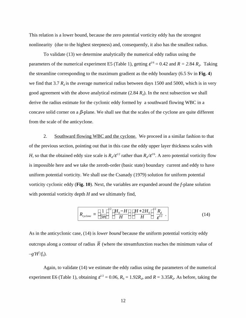
2. Southward flowing WBC and the cyclone. We proceed in a similar fashion to that

of the previous section, pointing out that in this case the eddy upper layer thickness scales with

H, so that the obtained eddy size scale is Rd /ε1/2 rather than Rd /ε1/6. A zero potential vorticity flow

is impossible here and we take the zeroth-order (basic state) boundary current and eddy to have

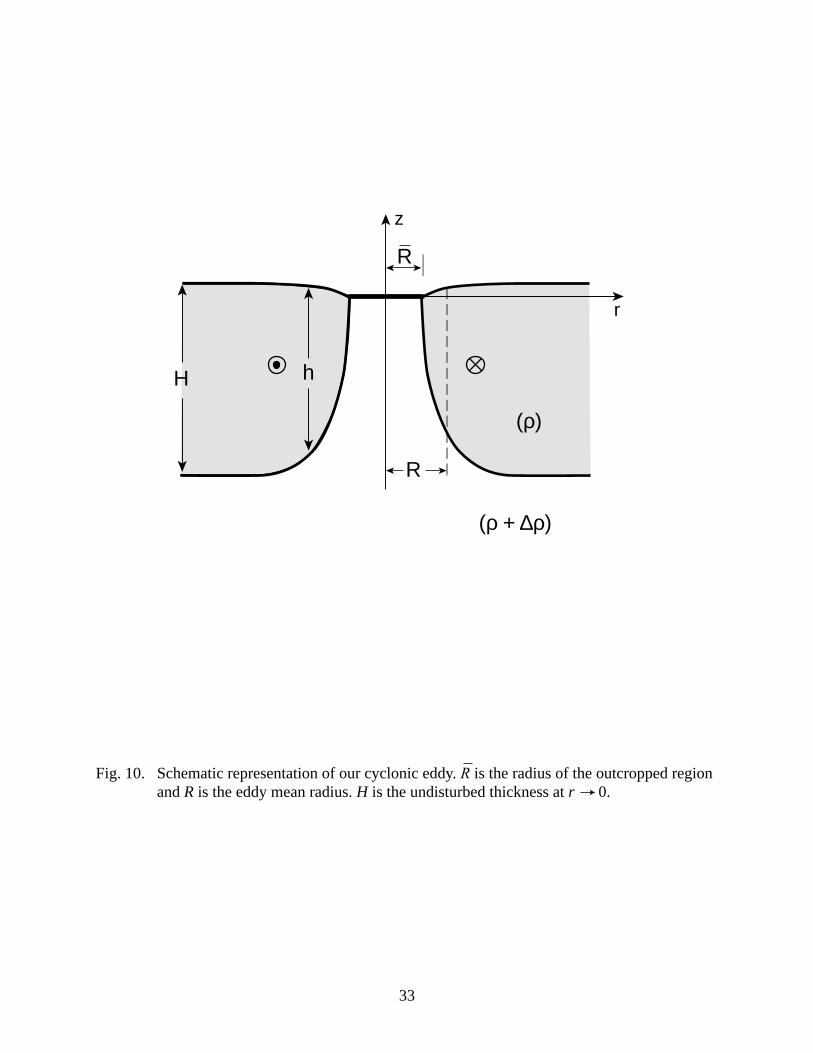
uniform potential vorticity. We shall use the Csanady (1979) solution for uniform potential

vorticity cyclonic eddy (Fig. 10). Next, the variables are expanded around the f-plane solution

with potential vorticity depth H and we ultimately find,

RH H

HH H

HR

cycloned .

/ /

/= π

−

+

13

21 2

0 0

1 2

1 2ε (14)

As in the anticyclonic case, (14) is lower bound because the uniform potential vorticity eddy

outcrops along a contour of radius R (where the streamfunction reaches the minimum value of

–g'H2/f0).

Again, to validate (14) we estimate the eddy radius using the parameters of the numerical

experiment E6 (Table 1), obtaining ε1/2 = 0.06, R0 = 1.92Rd, and R = 3.35Rd. As before, taking the

13

streamline corresponding to the maximum gradient as the eddy boundary in E6 (3.5 Sv in

Fig. 7), we estimate 4.28Rd as the average numerical radius between days 1500 and 5000. This is

in a fair-to-good agreement with the analytical estimate (3.35Rd).

4. The collision problem

In this section we will examine the full collision problem of two opposing WBCs on a β-

plane (Fig. 11). Recall that, as in the earlier case mentioned above, β is crucial here as, for an

analogous f-plane situation, Agra and Nof (1993) showed that net momentum flux of the

colliding currents is balanced, i.e., no eddies are necessary for the f-plane momentum balance to

hold.

a. Formulation

We shall denote the northward flowing current as the ”main current ”and the southward

flowing one as the “counter current.” At some point on the western boundary the currents collide

and veer offshore as a joined current. We place the origin of our coordinate system at the

collision (stagnation) point on the western boundary and assume that, far east of the western

boundary and a few Rossby radii away from the dividing streamline the upper layer thickness

has a value of Hs in the main current (south) side and Hn in the counter current (north) side.

Assuming a steady state and integrating (after multiplying by h) the steady, inviscid nonlinear

y-momentum equation over the fixed region S bounded by ABCDA we get,

hv dx hv dxg

h y h y dx

dxdy

LnLs

Net momentum flux

s n

L

essure term

S

term

2 2

00

2 2

0

2

20 0

0

− + −[ ]

− =

∫∫ ∫

∫∫1 2444 3444 1 244444 344444

1 2444 3444

'

( , ) ( , )

,

Pr

β ψ

β

(15)

14

where Ls and Ln are the main current and counter current widths, S is the integration region

bounded by ABCDA (Fig. 11), L2 is the zonal width of S, and ys and yn are the y-coordinates of

the southern and northern boundaries of S.

To apply our previous analytical approach to the collision problem, we divide the

integration region into two sub-domains S+ and S–, north and south of ψ = 0, respectively.

hv dxg

H h dx dxdyLs L

S

2

002 2

0

2

20 0+ −[ ] − − =∫ ∫ ∫∫ ∞

−

'( , ) ( ) ,φ β ψ ψ (16)

and,

hv dxg

h H dx dxdyLn L

S

2

0

202

0

2

20 0+ −[ ] − − =∫ ∫ ∫∫ ∞

+

'( , ) ( ) ,φ β ψ ψ (17)

where H0 is the upper layer thickness on ψ = 0 as x → ∞ , and ψ∞ (a function of y only) is the

limit of φ as x → ∞. As expected, the two have a mutual term g

h x dx y xL'

( , ) , ( )2

2

0

2

φ φwhere =∫ is a

Cartesian representation of the curve φ = 0. We shall see in the next subsection that the second

term in (14) and (15) is approximately zero and that, consequently, our solid corner solutions

will also be valid here.

b. Numerical simulations

The parameters for the collision experiment E9 on a β-plane (Table 1) are identical to

those used for experiments E5 and E6 for the concave corner. Fig. 12 shows contour plots of the

upper layer thickness and streamfunction for experiment E9 at day 2500. It is evident that an

anticyclonic eddy is formed south of the joined offshore current and cyclonic eddy north of it.

Fig. 13 shows the upper layer thickness along the western boundary (upper panel) and along the

ψ = 0 streamfunction (lower panel). Note the similarity with Figs. 5 and 8 for the β-plane

experiments E5 and E6. The pressure force points in the same direction as the momentum flux

(in each of the individual sub-domains). Therefore, eddies are necessary in order to reach the

15

integrated momentum balances in S- and S+

individually. The average value for the upper layer

thickness on the zero streamfunction is 270.8 m while the mean value outside the eddy influence

area is 271 m (Fig. 13), showing that, even in the collision problem, the condition that the second

term in (16) and (17) vanishes is valid.

Fig. 14 shows the numerical estimates for the terms in (15) (upper panel), (16) (middle

panel), and (17) (lower panel). In all the cases the inviscid momentum balances hold. The

analytical estimates for the flow inside a concave corner can also be used here, by considering

the ψ = 0 streamfunction as a “wall” dividing the basin in two parts (the main current side and

the counter current side). Taking the –4 Sv streamline as the boundary of the cyclonic eddy and

the 6.5 Sv streamline as the boundary of the anticyclonic eddy (Fig. 12) we estimate (from the

numerics) an average radius of 4.5 Rdn [where Rdn =(g'Hn)1/2/f0] and 3 Rds [where Rds = (g'Hn)

1/2/f0].

With differences of less than 26%, we can say that these are in decent agreement with the

analytical estimates (of 3.35 Rdn and 2.84 Rds). Recall that these analytical estimates neglect the

second terms in (16) and (17).

In the next section we shall apply the theory of the collision of opposing flowing WBC

on a β-plane to the equatorial western Pacific; in this scenario, the NGCC is the “main current”

and the MC is the “counter current.”

5. Discussion and summary

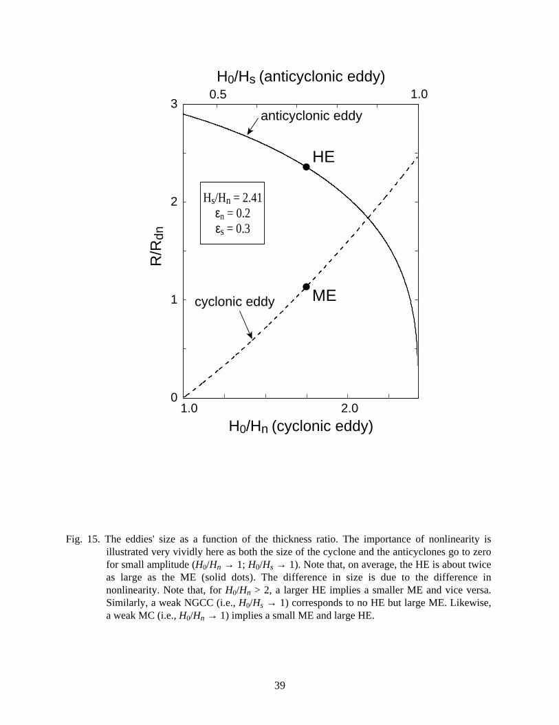
The sizes of the eddies as a function of their thickness are shown in Fig. 15. We see that

in the linear limit (H0/Hn → 1 for the cyclone and H0/Hs → 1 for the anticyclone) both eddies

disappear. This is consistent with Morey et al. (1999) who showed that both eddies do not exist

in the linear case. Fig. 15 also displays the ME and HE radii. We obtained these values by taking

16

26 Sv for the MC transport and 22 Sv for the NGCC transport. Approximately 11 Sv from the

MC and 1 Sv from the SEC flow into the ITF. Using the values calculated by Nof (1996) for the

offshore upper layer thicknesses of the colliding currents (Hn = 97.83 m for the MC and Hs = 235

.32 m for the NGCC) we obtain H0 = 170 m. Substituting the values of Hs, Hn, and H0 into (11)

and (14), we get a radius of 1.144 Rdn for the Mindanao eddy (where Rdn = 110 km and εn = 0.2)

and a radius of 1.52 Rds for the Halmahera eddy (where Rds = 171 km and εn = 0.3). The estimated

radii compare very well with the observations (Lukas et al.1991; Kashino et al. 1999) of 1.136

Rdn (125 km) for the Mindanao eddy and between 1.37 Rds and 1.46 Rds (between 235 and 250

km) for the Halmahera eddy.

A fundamental question to ask is what causes the factor of two or so difference in the

calculated eddy sizes. The answer is primarily nonlinearity which manifests itself via both large

momentum fluxes and large difference between the thickness north and south of the NECC (Hn

and Hs). Variations in the composition of the ITF would, of course, lead to changes in H0, and

consequently, to variations in the relative sizes of the eddies.

Figs. 4 and 8 are the most elucidating of our analysis because they highlight the profound

difference between an f-plane and a β-plane flow in a concave solid corner. In the f-plane case

there is no eddy and the flow is diagonally symmetric while in the β-plane case there is lack of

symmetry and a stationary eddy is attached to the curving flow. The momentum balance

relations (6) for nonlinear WBC in concave solid corner shows that, on an f-plane, no eddy is

necessary because the pressure force (produced by the difference between the upper layer

thickness) balances the current’s momentum flux. On a β-plane, on the other hand, the pressure

force and the boundary current momentum force point in the same direction. Consequently, a

permanent eddy is necessary to produce an opposing β-force leading to the required momentum

balance. Nonlinearities are of equal fundamental importance because in the linear limit the

boundary current momentum flux approaches zero so that no eddy is established. This is why

Morey’s et al. (1999) experiments show that there are no eddies when the nonlinearity is very

small. In this sense our work has some similarity to the much larger (basin scale) re-circulation

17

regions which also show up only when nonlinearity is present (i.e., they are not present in the

limit of a frictional WBC and a Sverdrup interior). The lower bound estimate for the radius of the

anticyclonic eddy is given by (13) and, similarly, the lower bound estimate for the radius of the

cyclonic eddy is given by (14).

Applying the collision theory for the MC and NGCC in the western equatorial Pacific

taking into account only the effective part of each current that participates in the collision

process (i.e., excluding the parts that form the ITF), we estimate a diameter of 252 km for the

ME and 520 km for the HE. These are in excellent agreement with the observed values of 250

km and between 470 and 500 km (Lukas et al.1991; Kashino et al. 1999). We show that the

difference between the two is primarily due to nonlinearity (Fig. 15), i.e., the stronger

momentum flux of the NGCC relative to that of the MC. This nonlinearity manifests itself in a

large difference in the thickness of the upper layer north and south of the NECC. An additional

aspect that explains some (~50%) of the difference in the size is the difference in the Coriolis

parameter (due to the different latitudes) which contributes to a larger Rossby radius in low

latitudes.

Also, note that, according to our solution (Fig. 14), a weaker MC and stronger NGCC

(i.e., H0/Hn → 1) implies smaller ME and larger HE. Similarly, a stronger MC and a weaker

NGCC (i.e., H0/Hs → 1) implies larger ME and smaller HE. This is in agreement with

Waworantu (1999) statements that in Dec-Fed there is almost no HE but the ME is large

(because the NGCC is very weak, i.e., H0/Hn → 1). In the fall, on the other hand, the HE is strong

and the ME is weak because the NGCC is strong (i.e., H0/Hn is small). These results are also

consistent with the reports of Lukas et al. 1991 and Kashino et al. 2001.

The above arguments show that the physical mechanism proposed here (i.e., that the

eddies are necessary to balance the nonlinear momentum flux of their parent currents, the

southward flowing MC and the northward flowing NGCC) are indeed responsible for the

formation of the ME and HE. Of course, our model does not describe all of the oceanic details as

it neglects motions below the upper layer as well as the inclination and complexity of the

18

coastline. These could, no doubt, alter our results but our findings are nevertheless informative as

they provide a first glance at the processes in question. We also point out that, although the ITF

plays a secondary role in our theory, its existence is essential for the formation of the cross

equatorial flow of the NGCC (see e.g., Arruda 2002, Nof 1998). Without the ITF there would be

no collision and no eddies. Consequently, it is not surprising that variations in the ITF transport

lead to variations of the relative sizes of the ME and the HE.

Acknowledgements

This study was supported by the Binational Science Foundation grant 96-105; National

Science Foundation grants OCE 9911324 and OCE 0241036; National Aeronautics and Space

Administration grants NAG5-7630 andNAG5-10860; and Office of Naval Research grant

N00014-01-0291.Wilton Z. Arruda was funded by “Conselho Nacional de Desenvolvimento

Científico e Tecnológico” (CNPq-Brazil) under grant 202436/91-8 and a fellowship from the

Inter-American Institute for Global Change Research (IAI) through South Atlantic Climate

Change Consortium (SACC). The authors would like to thank Dr. Nobuo Suginohara for his

helpful comments and careful reading of the manuscript. We also thank Steve Morey and Jay

Shriver for making additional runs of their linear model.

19

Appendix. List of Symbols and Acronyms

B Bernoulli function, g'h + (u2 + v2)/2

f Coriolis parameter (f0 + βy)

g' Reduced gravity, g∆ρ/ρ

h Upper layer thickness

H Undisturbed interior upper layer thickness (replaced by either Hn or Hs for the

collision problem); see Fig. 2

H0 Upper layer thickness on the zonal wall as x → ∞ (Fig. 3)

h Upper layer thickness at the center of the anticyclonic eddy

Hmax Upper layer thickness at the corner (Fig. 3)

Hn ,Hs Upper layer thicknesses at fixed latitudes in the counter current side and main

current side (Fig. 11)

L Boundary current width (Fig. 2)

L2 Width of square domain S (Fig. 2)

Ln Counter current width (Fig. 11)

Ls Main current width (Fig. 11)

R Eddy radius

R Radius of the outcropped region in the cyclonic eddy (Fig. 10)

Rd Rossby radius of deformation, (g'H)1/2/f0

Rdn Rossby radius of deformation, (g'Hn)1/2/f0

Rds Rossby radius of deformation, (g'Hs)1/2/f0

Rde Rossby deformation radius of the anticyclonic eddy, (g'He)1/2/f0

S Integration area bounded by dashed rectangle in Fig. 2

S+ , S– Subsets of S such that y ≥ 0 and y ≤ 0, respectively

u,v Velocity components in Cartesian coordinates

vθ Orbital velocity in the eddy

20

ys,yn Latitudes of the southern and northern boundaries of S (Figs. 2 and 11)

β Variation of the Coriolis parameter with latitude

ε Small parameter equal to βRd/f0

φ Cartesian representation of the dividing streamline in the collision problem

ρ, ∆ρ Density and density difference between the layers

υ Frictional coefficient

ψ Streamfunction (defined by ψy = –uh ; ψx = –vh

ψ∞ Limit of ψ as x → ∞

ψ (ψ – ψ∞)

ADCP Acoustic Doppler Current Profiler

HE Halmahera eddy

ITF Indonesian throughflow

MC Mindanao Current

ME Mindanao eddy

NECC North Equatorial Counter Current

NGCC New Guinea Coastal Current

NGCUC New Guinea Coastal Undercurrent

SEC South Equatorial Current

WBC Western Boundary Current

21

References

Agra, C. and D. Nof, 1993: Collision and separation of boundary currents. Deep-Sea Res. I, 40,

2259-2282.

Anderson, D. L. T. and D. W. Moore, 1979: Cross-equatorial inertial jets with special relevance

to very remote forcing of the Somali Current. Deep-Sea Res., 26, 1-22.

Arakawa, A., 1966. Computational design for long-term numerical integration of the equations

of fluid motion. Two dimensional incompressible flow. Part I, J. Comput. Phys., 1, 119-

143.

Arruda, W., 2002: Eddies along western boundaries. Ph.D. Dissertation, Florida State University,

90 pp.

Arruda, W., D. Nof and J. J. O’Brien, 2003: The Ulleung eddy owes its existence to β and

nonlinearities. Deep-Sea Res. II, submitted.

Bleck, R. and D. Boudra, 1981: Initial testing of a numerical ocean circulation model using a

hybrid, quasi-isopycnic vertical coordinate. J. Phys. Oceanogr., 11, 744-770.

Bleck, R. and D. Boudra, 1986: Wind-driven spin-up in eddy-resolving ocean models

formulated in isopycnic and isobaric coordinates. J. Geophys. Res., 91, 7611-7621.

Bleck, R. and L. T. Smith, 1990: A wind-driven isopycnic coordinate model of the North and

Equatorial Atlantic Ocean, 1, Model development and supporting experiments. J.

Geophys. Res., 95, 3273-3285.

Cannon, G. A., 1970: Characteristics of waters east of Mindanao, Philippine Islands, August,

1965. In The Kuroshio, A Symposium on the Japan Current, ed. J.C. Marr, East-West

Center, Honolulu, Hawaii, pp. 205-211.

Cantos-Figuerola, A., and B. A. Taft, 1983: The South Equatorial Current during 1979-80

Hawaii-Tahiti Shuttle. Trop. Ocean. Atmos. Newslett., 19, 6-8.

Cessi, P., 1990: Recirculation and separation of boundary currents. J. Mar. Res., 48, 1-35.

Cessi, P., 1991: Laminar separation of colliding western boundary currents. J. Mar. Res., 49,

697-717.

22

Church, J. A., and F. M. Boland, 1983: A permanent undercurrent adjacent to the Great Barrier

Reef, J. Phys. Oceanogr., 13, 1747-1749.

Csanady, G. T., 1979: The birth and death of a warm-core ring. J. Geophys. Res.,84, 777-780.

Ffield, A. and A. L. Gordon, 1992: Vertical Mixing in the Indonesian Thermocline. J. Phys.

Oceanogr., 22, 184-195.

Gordon, A. L., 1986: Inter-ocean exchange of thermocline water. J. Geophys. Res.,91, 5037-5050.

Gouriou, Y. and J. Toole, 1993: Mean circulation of the upper layers of the Western Equatorial

Pacific Ocean. J. Geophys. Res., 98, 22495-22520.

Kashino, Y., H. Watanabe, B. Herunadi, M. Aoyama, and D. Hartoyo, 1999: Current variability

at the Pacific entrance of the Indonesian Throughflow. J. Geophys. Res., 104, 11021-

11035.

Kashino, Y., E. Firing, P. Hacker, A. Sulaiman, and Lukiyanto, 2001: Currents in the Celebes

and Lakulu Seas. Geophys. Res. Letters, 28(7), 1263-1266.

Kendall, T. R., 1969: Net transport in the western equatorial Pacific Ocean. J. Geophys. Res..,

74, 1388-1369.

Kessler, W. S. and B. A. Taft, 1987: Dynamic heights and zonal geostrophic transports in the

central Pacific during 1979-1984. J. Phys. Oceanogr., 7, 97-122.

Kundu, P. K., 1990: Fluid Mechanics. Academic Press, 638 pp.

Lebedev, I. and D. Nof, 1996: The drifting confluence zone. J.Phys.Oceanogr., 26, 2429-2448.

Lebedev, I. and D. Nof, 1997: Collision of boundary currents: Beyond a steady state. Deep-Sea

Res., 44, 771-791.

Lukas, R., E. Firing, P. Hacker, P.L. Richardson, C. A. Collins, R. Fine and R. Gammon, 1991:

Observations of the Mindanao Current during the Western Equatorial Pacific Ocean

Circulation Study. J. Geophys. Res., 96, 7,089-7,104.

Masuzawa, J., 1968: Second cruise for CSK, Ryofu Maru, January to March 1968. Oceanogr.

Mag., 20, 173-185.

23

Masuzawa, J., 1969: The Mindanao Current. Bull. Japan. Soc. Fish. Oceanogr., 99-104.

Morey, S. L, J. F. Shriver and J. J. O'Brien, 1999: The effects of Halmahera on the Indonesian

throughflow. J. Geophys. Res., 104 (C10), 23281-23296.

Nof, D., 1996: What controls the origin of the Indonesian throughflow? J. Geophys. Res., 101,

12301-12314.

Nof, D., 1998: The ‘separation formula’ and its application to the Pacific Ocean. Deep-Sea

Res. I, 45, 2011-2033.

Nof, D. and T. Pichevin, 1999: The establishment of the Tsugaru and the Alboran gyres. J. Phys.

Oceanogr., 29, 39-54.

Orlanski, I., 1976: A simple boundary condition for unbounded hyperbolic flows. J. Comp.

Phys., 21, 251-269.

Qu, T., H. Mitsudera and T. Yamagata, 1999: A climatology of the circulation and water mass

distribution near the Philippine Coast. J. Phys. Oceanogr., 29, 1488-1505.

Takahashi, T., 1959: Hydrographical researches in the western equatorial Pacific. Mem. Faculty

Fish. Kagoshima Univ., 7, 141-147.

Toole, J. M., E. Zou and R. C. Millard, 1988: On the circulation of the upper waters in the

western equatorial Pacific Ocean. Deep-Sea Res., 35, 1451-1482.

Toole, J.M., R.C. Millard, Z. Wang, and S. Pu, 1990: Observations of the Pacific North

Equatorial Current Bifurcation at the Philippine Coast. J. Phys. Oceanogr., 20, 307-318.

Wyrtki, K., 1956: The subtropical lower water between the Philippines and Iran (New Guinea).

Mar. Res. Indonesia, 1, 21-52.

Wyrtki, K., 1961: Physical oceanography of the Southeast Asian waters. NAGA Rep., 2, 195 pp.

Wyrtki, K., and B. Kilonsky, 1984: Mean water and current structure during Hawaii-to-Tahiti

Shuttle Experiment. J. Phys. Oceanogr., 14, 242-254.

24

ME

NEC

NGCC

NECC

MC

HE

Molucca

Sea

Cera

m S

ea

Pacific Ocean

NEW

GUINEA

10N

5N

EQ

5S125E 130E 135E 140E

Fig. 1. The flow pattern in the western equatorial Pacific (adapted from Ffield and Gordon 1992). The Mindanao eddy (ME) and the Halmahera eddy (HE) are semi-permanent and do not usually drift away from their generation area. Dashed arrows denote the southern part of the Indonesian throughflow (ITF).

25

z z

A

A

B

C

C

D

D

y = ys

y = yn

y = 0

y = 0B

h = H

h = H

x

x

N N

h

Inflow profile

h

Inflow profile

x

y y

x

Fig. 2. Schematic diagram of the solid corner model. Upper panels: A northward (southward) flowing western boundary current (WBC) encountering a zonal wall. H is the upper layer far east from the western boundary on a latitude a few Rossby radii away from the zonal wall. Lower panels: Vertical cross-section of the approaching northward (southward) flowing WBC.

(ρ)

(ρ)

(ρ)

(ρ)

(ρ + ∆ρ) (ρ + ∆ρ)

L2

Anticyclonic eddy

Cycloniceddy

Top View

Side View

L2

L ~ O

(Rd )

L ~

O(R

d)

26

Fig. 3. Schematic three-dimensional diagram of the upper layer thicknesses on the boundaries of a northward flowing western boundary current on an f-plane (upper panel) and on a -plane (lower panel). Note that the upstream near wall thickness is greater in the -plane case. This is why the eddy is established (see text).

(ρ + ∆ρ)

(ρ)

H0

h

z

z

y

x

x

h

f - plane

(ρ + ∆ρ)

(ρ)

- plane

Hmax

Hmax

H0

H0Western boundary

Western boundary

Zonal wall

Zonal wall

β

ββ

27

Upper layer thickness (m) Upper layer thickness (m)

Streamfunction (Sv) Streamfunction (Sv)

- plane

x

x

x

x

y y

y y

Fig. 4. Upper layer thickness contours (upper left) and streamfunction contours (lower left) for the f-plane experiment E1 (Table 1) at day 2500; upper layer thickness contours (upper right) and streamfunction contours (lower right) for the -plane experiment E5 (Table 1) at day 2500. The contour spacing is 20 m for the upper layer thickness and 15 Sv for the streamfunction. The axis marks are 10 grid points (75 km) apart. Areas within the closed contours are shaded.

4.5

6.5

8.5

3.5

4.5

330

350

380

350

f - plane

f - plane

β

- planeβ

β

410

365

28

x x

y y

hh

h h

290

280

270

290

280

270

290

280

270

290

280

270

f - plane

f - plane

h along the western boundary h along the western boundaryh

(m)

h (m

)

h (m

)h

(m)

Fig. 5. The f-plane upper layer thickness h (in meters) along the western boundary (upper left) and along the zonal wall (lower left) at day 2500; -plane upper layer thickness h (in meters) along the western boundary (upper right) and along the zonal wall (lower right) at day 2500. Shaded area is the upper layer. The horizontal axis marks are 10 grid points (75 km) apart.

- planeβ

- planeβ

β

29

0 1000 2000 3000 4000 5000

0

1

2

3

4

5

Days

0 1000 2000 3000 4000 5000 0.2

0.1

0

0.1

0.2

Days

Comparison of momentums (f - plane)

Comparison of momentums (f - plane)

Fig. 6. Terms of the momentum balance (9) computed from the f-plane experiment E1

(upper panel, and the -plane experiment E5 (lower panel). Note that, by day 500

for the f-plane run and day 800 for the -plane run, the steady state balance holds.

pressure term

pressure termminus pressure term

minus -term

WBC momentum flux

WBC momentum fluxx

107

m4 s

-2x

107

m4 s

-2

ββ

β

minus -term plus pressure term β

30

200

215

200

215140

185

170

-2.5

-2.5

-1.5

-4

-3

f - plane

f - plane

y y

y y

xx

xx

Fig. 7. Upper layer thickness contours (upper left) and streamfunction contours (lower left) for the f-plane experiment E2 (Table 1) at day 2500; upper layer thickness contours (upper right) and streamfunction contours (lower right) for the -plane experiment E6 (Table 1) at day 2500. The contour spacing is 20 m for the upper layer thickness and 15 Sv for the streamfunction. The axis marks are 10 grid points (75 km) apart. Areas within the closed contours are shaded. Note the diagonal symmetry of the f-plane runs and the diagonal asymmetry of the -plane runs.

- planeβ

- planeβ

β

β

31

y y

x x

280

275

270

265

280

275

270

265

280

275

270

265

280

275

270

265

f - plane

f - plane

Fig. 8. The f-plane upper layer thickness h (in meters) along the western boundary (upper left) and along the zonal wall (lower left) at day 2500; -plane upper layer thickness along the western boundary (upper right) and the zonal wall (lower right) at day 2500. Shaded area is the upper layer. The horizontal axis marks are 10 grid points (75 km) apart.

h

hh

h

h along the western boundary h along the western boundary

h along the zonal wallh along the zonal wall

h (m

)h

(m)

h (m

)h

(m)

- planeβ

- planeβ

β

32

0 1000 2000 3000 4000 5000

- 0.1

0

0.1

Days

0 1000 2000 3000 4000 5000 - 3

- 2

- 1

0

Days

WBC momentum flux

pressure term

minus pressure term

pressure term

minus term minus pressure term

WBC momentum flux

Comparison of momentums (f - plane)

Comparison of momentums ( - plane)

Fig. 9. Terms of the momentum balance (13) computed from the f-plane experiment E2 (upper panel), and the -plane experiment E4 (lower panel). Note that the f-plane run reaches a steady state right away [within a period of O(f -1)] while the -plane run takes 500 days to reach a steady state.

x 10

7 m

4 s-2

x 10

7 m

4 s-2

β

β minus term

ββ

β

33

R

r

z

H

(ρ)

(ρ + ∆ρ)

h

R

Fig. 10. Schematic representation of our cyclonic eddy. R is the radius of the outcropped region and R is the eddy mean radius. H is the undisturbed thickness at r 0.

34

Ny

x

A

E

Ls

Ls

L2

D

B

F

Cy = yn

h = Hn

h = Hsy = ys

y = 0

Cycloniceddy

Anticycloniceddy

ψ = 0

(ρ)

Fig. 11a. Schematic top view of the collision of a northward flowing boundary current (maincurrent) and a southward flowing boundary current (counter current) on a β-plane.

After the collision the two currents merge into a joined offshore current. East of thewestern boundary and a few Rossby radii away from the dividing streamline (y = 0)the upper layer thickness is Hs and Hn (where the subscripts "s" and "n" denote"south" and "north".

35

H0

f = f0

(ρ)

(ρ + ∆ρ)

h

zy

Hs

Hn

x

Western boundary

Eastward flowing

joint current

(NECC)

Fig. 11b. A three-dimensional view of the long wall and long-jet thicknesses.

MC

NGCC

36

Upper layer thickness (m) Streamfunction (Sv)

200

140

170

350395

275

-4.5-2.5

4.5

5.5

7.5

x x

yy

Fig. 12. Upper layer thickness contours (left panel) and streamfunction contours (right panel) for the collision experiment on a -plane at day 2500. The axis marks are 10 grid points (75 km) apart. Areas within closed contours are shaded. Recall that no eddies are produced in the f-plane case (see Fig. 5 in Lebedev and Nof 1997).

E8 E836

5

β

37

h

h

290

280

270

h along ψ = 0

h(m

)

285

275

265

Fig. 13. Upper layer thickness h (in meters) along the western boundary (upper panel) and along the offshore branch of ψ = 0 (lower panel) for the collision experiment E8 at day 2500.

E8

E8

y

x

h along the western boundary

38

0 2000 4000 6000 8000 10000

0

1

Days

0 2000 4000 6000 8000 10000

0

1

2

3

4

Days

0 2000 4000 6000 8000 10000

- 2

- 1

0

counter current momentum flux

main current momentum flux

net momentum flux

minus term minus pressure term

Days

Comparison of momentums (Main current)

Comparison of momentums (Counter current)

Fig. 14. Momentum balance for the area containing both colliding currents (upper panel); momentum balance for the area south of the zero streamfunction (middle panel); momentum balance for the area north of the zero streamfunction (lower panel). All terms were computed from experiment E8.

x 10

7 m

4 s-2

x 10

7 m

4 s-2

x 10

7 m

4 s-2

β

minus term minus pressure termβ

minus term minus pressure termβ

minus term β

minus term β

minus term β

pressure term

pressure term

pressure term

Comparison of momentums (Collision)

39

1.0 2.0 0

1

2

3

HE

ME

R/R

dn

H0/Hn (cyclonic eddy)

H0/Hs (anticyclonic eddy)0.5 1.0

Fig. 15. The eddies' size as a function of the thickness ratio. The importance of nonlinearity is illustrated very vividly here as both the size of the cyclone and the anticyclones go to zero for small amplitude (H0/Hn → 1; H0/Hs → 1). Note that, on average, the HE is about twice as large as the ME (solid dots). The difference in size is due to the difference in nonlinearity. Note that, for H0/Hn > 2, a larger HE implies a smaller ME and vice versa. Similarly, a weak NGCC (i.e., H0/Hs → 1) corresponds to no HE but large ME. Likewise, a weak MC (i.e., H0/Hn → 1) implies a small ME and large HE.

cyclonic eddy

anticyclonic eddy

Hs/Hn = 2.41εn = 0.2εs = 0.3