The Michelson Interferometer - CWSEI · The Michelson Interferometer ... Using the WinTV2000...

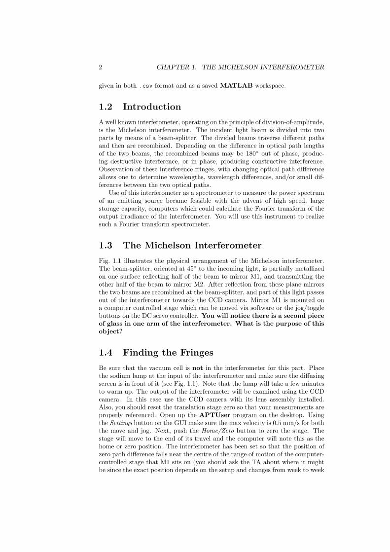
Chapter 1

The MichelsonInterferometer

1.1 Prelab

In this lab you have to find the position of mirror M1 (see Fig. 1.1) such thatthe optical path length from the beam splitter to M1 and back is identical tothe optical path length from the beam splitter to M2 and back again. Thisspecial position insures the path length difference is zero and is referred to asthe “zero path length” ZPL. As the position of M1 approaches the position ofZPL, you will observe that the periodicity of the circular interference fringes(which are circular for the lamps - sodium and the white light) becomes largerand they are the largest at the ZPL (see Fig. 1.2). Explain qualitatively whythis is. Next, model this situation numerically. Derive an expression for theinterference pattern as a function of z from two spherical waves where the sourcesare separated on the z-axis by a distance d apart (representing the two differentbeam paths in the interferometer). Hint: write down the electric field amplitudes(U1 and U2) from two spherical wave sources and compute the total intensityI = |U1 + U2|2. Plot the total intensity (i.e. interference pattern) for twodifferent separations d. Comment on the change of the ring periodicity as dgets smaller. Also, for a given d comment on the ring periodicity as you moveradially away from the z-axis along x or y.

In this lab, you will also use the interferometer to measure the index ofrefraction of air by putting a vacuum cell in between the beamsplitter andmirror M2 and measuring the additional phase shift acquired when you slowlyintroduce air into the evacuated cell. How many times does the beam traversethe cell in the interferometer? Compute the total optical path length differencefor light at 632.8 nm with and without air in a vacuum cell 10 cm in length.What is the expected number of fringes that will pass as air is leaked into a cellof this length initially under a perfect vacuum?

Also, before doing this lab, you should prepare a MATLAB .m file whichperforms the analysis outlined in section 1.10.2. The code for this MATLABscript is spelled out in this section, and you should test it with the sampleFourier spectroscopy data (of a white light spectrum) provided on the opticslab webpage next to the link to the .pdf of this document. The sample data is

1

2 CHAPTER 1. THE MICHELSON INTERFEROMETER

given in both .csv format and as a saved MATLAB workspace.

1.2 Introduction

A well known interferometer, operating on the principle of division-of-amplitude,is the Michelson interferometer. The incident light beam is divided into twoparts by means of a beam-splitter. The divided beams traverse different pathsand then are recombined. Depending on the difference in optical path lengthsof the two beams, the recombined beams may be 180◦ out of phase, produc-ing destructive interference, or in phase, producing constructive interference.Observation of these interference fringes, with changing optical path differenceallows one to determine wavelengths, wavelength differences, and/or small dif-ferences between the two optical paths.

Use of this interferometer as a spectrometer to measure the power spectrumof an emitting source became feasible with the advent of high speed, largestorage capacity, computers which could calculate the Fourier transform of theoutput irradiance of the interferometer. You will use this instrument to realizesuch a Fourier transform spectrometer.

1.3 The Michelson Interferometer

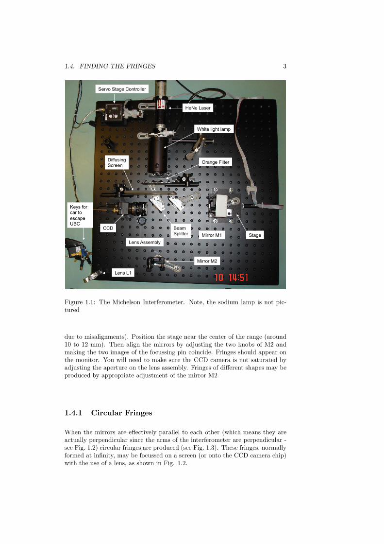
Fig. 1.1 illustrates the physical arrangement of the Michelson interferometer.The beam-splitter, oriented at 45◦ to the incoming light, is partially metallizedon one surface reflecting half of the beam to mirror M1, and transmitting theother half of the beam to mirror M2. After reflection from these plane mirrorsthe two beams are recombined at the beam-splitter, and part of this light passesout of the interferometer towards the CCD camera. Mirror M1 is mounted ona computer controlled stage which can be moved via software or the jog/togglebuttons on the DC servo controller. You will notice there is a second pieceof glass in one arm of the interferometer. What is the purpose of thisobject?

1.4 Finding the Fringes

Be sure that the vacuum cell is not in the interferometer for this part. Placethe sodium lamp at the input of the interferometer and make sure the diffusingscreen is in front of it (see Fig. 1.1). Note that the lamp will take a few minutesto warm up. The output of the interferometer will be examined using the CCDcamera. In this case use the CCD camera with its lens assembly installed.Also, you should reset the translation stage zero so that your measurements areproperly referenced. Open up the APTUser program on the desktop. Usingthe Settings button on the GUI make sure the max velocity is 0.5 mm/s for boththe move and jog. Next, push the Home/Zero button to zero the stage. Thestage will move to the end of its travel and the computer will note this as thehome or zero position. The interferometer has been set so that the position ofzero path difference falls near the centre of the range of motion of the computer-controlled stage that M1 sits on (you should ask the TA about where it mightbe since the exact position depends on the setup and changes from week to week

1.4. FINDING THE FRINGES 3

Mirror M2

Lens L1

CCD

Lens Assembly Stage

Servo Stage Controller

HeNe Laser

Diffusing Screen

Orange Filter

Keys for car to escape UBC

Mirror M1 Beam Splitter

White light lamp

Figure 1.1: The Michelson Interferometer. Note, the sodium lamp is not pic-tured

due to misalignments). Position the stage near the center of the range (around10 to 12 mm). Then align the mirrors by adjusting the two knobs of M2 andmaking the two images of the focussing pin coincide. Fringes should appear onthe monitor. You will need to make sure the CCD camera is not saturated byadjusting the aperture on the lens assembly. Fringes of different shapes may beproduced by appropriate adjustment of the mirror M2.

1.4.1 Circular Fringes

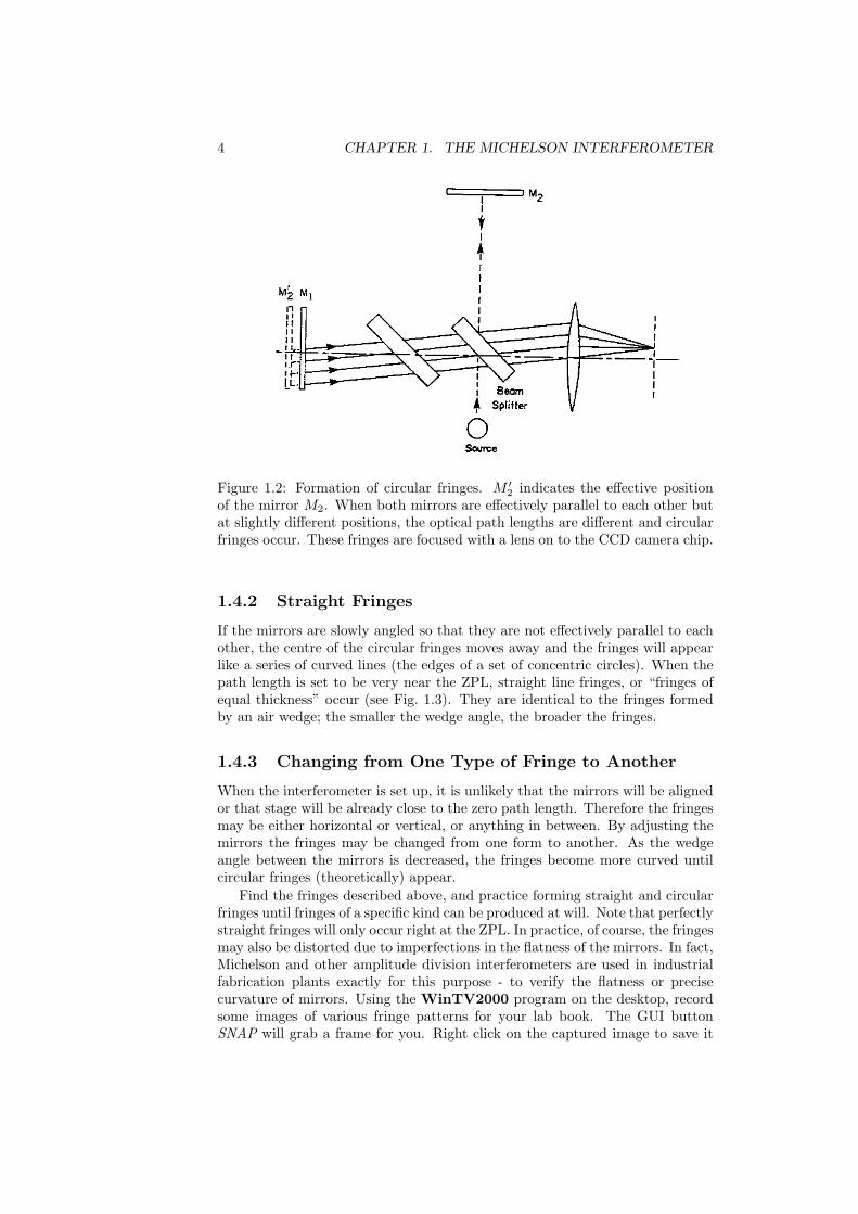
When the mirrors are effectively parallel to each other (which means they areactually perpendicular since the arms of the interferometer are perpendicular -see Fig. 1.2) circular fringes are produced (see Fig. 1.3). These fringes, normallyformed at infinity, may be focussed on a screen (or onto the CCD camera chip)with the use of a lens, as shown in Fig. 1.2.


Figure 1.2: Formation of circular fringes. M ′2 indicates the effective positionof the mirror M2. When both mirrors are effectively parallel to each other butat slightly different positions, the optical path lengths are different and circularfringes occur. These fringes are focused with a lens on to the CCD camera chip.

1.4.2 Straight Fringes

If the mirrors are slowly angled so that they are not effectively parallel to eachother, the centre of the circular fringes moves away and the fringes will appearlike a series of curved lines (the edges of a set of concentric circles). When thepath length is set to be very near the ZPL, straight line fringes, or “fringes ofequal thickness” occur (see Fig. 1.3). They are identical to the fringes formedby an air wedge; the smaller the wedge angle, the broader the fringes.

1.4.3 Changing from One Type of Fringe to Another

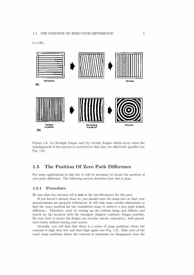
When the interferometer is set up, it is unlikely that the mirrors will be alignedor that stage will be already close to the zero path length. Therefore the fringesmay be either horizontal or vertical, or anything in between. By adjusting themirrors the fringes may be changed from one form to another. As the wedgeangle between the mirrors is decreased, the fringes become more curved untilcircular fringes (theoretically) appear.

Find the fringes described above, and practice forming straight and circularfringes until fringes of a specific kind can be produced at will. Note that perfectlystraight fringes will only occur right at the ZPL. In practice, of course, the fringesmay also be distorted due to imperfections in the flatness of the mirrors. In fact,Michelson and other amplitude division interferometers are used in industrialfabrication plants exactly for this purpose - to verify the flatness or precisecurvature of mirrors. Using the WinTV2000 program on the desktop, recordsome images of various fringe patterns for your lab book. The GUI buttonSNAP will grab a frame for you. Right click on the captured image to save it

1.5. THE POSITION OF ZERO PATH DIFFERENCE 5

to a file.

Figure 1.3: (a) Straight fringes and (b) circular fringes which occur when themisalignment of the mirrors is corrected so that they are effectively parallel (seeFig. 1.2).

1.5 The Position Of Zero Path Difference

For some applications in this lab, it will be necessary to locate the position ofzero path difference. The following section describes how this is done.

1.5.1 Procedure

Be sure that the vacuum cell is not in the interferometer for this part.If you haven’t already done so, you should reset the stage zero so that your

measurements are properly referenced. It will take some careful adjustment tofind the exact position for the translation stage to achieve a zero path lengthdifference. Therefore, start by setting up the sodium lamp and diffuser andsearch for the location with the strongest (highest contrast) fringes possible.Do your best to insure the fringes are circular (nicely concentric), well spaced,and clearly defined during your search.

Actually, you will find that there is a series of stage positions where thecontrast is high then low and then high again (see Fig. 1.6). Take note of theexact stage positions where the contrast is minimum (or disappears) near the


stage position where the contrast appears best. You will next look systematicallyand precisely between each of these minima for the ZPL using the white lightsource.

Another sign that you are near the zero path length difference is that theradius of curvature of the circular fringes is the largest. Why is that? At thislocation, you should be within a fraction of one millimeter from the zero pathlength difference. To look for changes of the radius of curvature as you movethe stage position, you could also look at the curvature of the straight fringeswith the mirrors slightly angled.

Be very careful not to bump the equipment at this stage since you can easilyknock the system out of alignment and ruin your pre-alignment work!

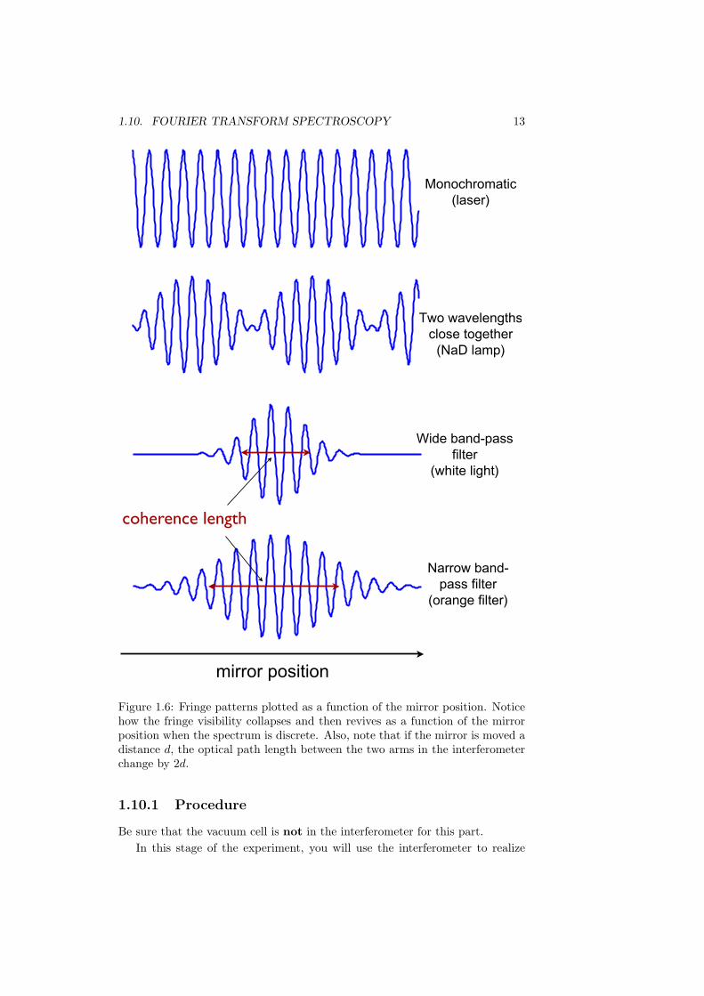
Now, replace the sodium lamp with the white light source. Note that theSodium lamp will be hot, so only grab it by the post. You will notice that fringesdo not appear. When using the white light source, they will only appear whenthe arms of the interferometer have equal path length. Why? What doesthis tell you about the “coherence length” of the white light source?What is the definition of the “coherence length?” You must adjust thestage until the path lengths are equal and fringes are observed.

Since finding the white light fringes is like looking for a needle in a haystack,you should cheat by using a narrow band filter with the white light source tofind fringes with filtered light and then remove the filter to find the zero pathlength difference with the white light. Why would this filter help? With thenarrow band filter in place, slowly scan the stage with the jog buttons to thepositions precisely between the minima you found before. When you finally trythe correct maxima, the stage will be near the ZPL and fringes will be observed.If you are spending more than 15 minutes without finding the white light fringes,ask a TA to help check you are doing everything correctly. At the point wherethe fringes appear with the unfiltered white light source, the stage is set forzero path length difference. Write down the stage position for future referenceand note the direction you approached the zero-path difference. The latter isimportant for mechanical backlash in the micrometer screw. Since you will beusing a MATLAB script to take data, and this script moves the stage forward(i.e. to higher values on the indexed stage), then backwards, then forward againback to the starting point, you should always approach from below your positionof zero-path length difference. The fringes will appear and disappear within 2µm, so you will probably have to adjust the max velocity and step distance ofthe stage so that you don’t go too fast and miss the appearance of the fringes.Also, use the actuator toggle with care since rapid changes in motion of thestage might also misalign the interferometer.

1.6 Calibration Of The Interferometer

Before the interferometer can be used to measure wavelengths it must firstbe calibrated. By “calibrated” we mean that the distance which the stageactually moves needs to be correlated to the approximate reading provided bythe computer.

1.6. CALIBRATION OF THE INTERFEROMETER 7

1.6.1 Procedure

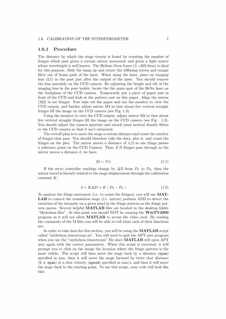
The distance by which the stage travels is found by counting the number offringes which pass given a certain mirror movement and given a light sourcewhose wavelength is well known. The Helium-Neon Laser (λ =632.8nm) is idealfor this purpose. Slide the lamp up and rotate the diffusing screen and orangefilter out of beam path of the laser. When using the laser, place an imaginglens (L1) in the post just after the output of the laser. You should removethe lens assembly on the CCD camera. By adjusting the height and tilt of theimaging lens in the post holder, locate the the main spot of the HeNe laser onthe backplane of the CCD camera. Temporarily put a piece of paper just infront of the CCD and look at the pattern cast on this paper. Align the mirror(M2) to see fringes. Now take out the paper and use the monitor to view theCCD output, and further adjust mirror M2 so that about five vertical straightfringes fill the image on the CCD camera (see Fig. 1.3).

Using the monitor to view the CCD output, adjust mirror M2 so that aboutfive vertical straight fringes fill the image on the CCD camera (see Fig. 1.3).You should adjust the camera aperture and attach some neutral density filtersto the CCD camera so that it isn’t saturated.

The overall plan is to move the stage a certain distance and count the numberof fringes that pass. You should therefore take the data, plot it, and count thefringes on the plot. The mirror moves a distance of λ/2 as one fringe passesa reference point on the CCD Camera. Thus, if N fringes pass through as themirror moves a distance d, we have,

2d = Nλ (1.1)

If the servo controller readings change by ∆D from D1 to D2, then themirror travel is linearly related to the stage displacement through the calibrationconstant K:

d = K∆D = K | D2 −D1 | (1.2)

To analyze the fringe movement (i.e. to count the fringes), you will use MAT-LAB to control the translation stage (i.e. mirror) position AND to detect thevariation of the intensity on a given pixel in the fringe pattern as the fringe pat-tern moves. Several helpful MATLAB files are located in the desktop folder“Michelson files”. At this point you should NOT be running the WinTV2000program as it will not allow MATLAB to access the video card. By readingthe comments of the M-files you will be able to tell what each of their functionsare.

In order to take data for this section, you will be using the MATLAB scriptcalled “michelson timestream.m”. You will need to quit the APT user programwhen you use the ”michelson timestream” file since MATLAB will open APTuser again with the correct parameters. When this script is executed, it willprompt you to click on the image the location where the fringe pattern is themost visible. The script will then move the stage back by a distance (span)specified in mm, then it will move the stage forward by twice that distance(2 x span) at a slow velocity (speed) specified in mm/s, and then it will movethe stage back to the starting point. To use this script, your code will look likethis


>> data = michelson_timestream(span, speed);

where span and speed are to be chosen by you, and the data will be returnedinto the array data. As an example, consider this code

>> data = michelson_timestream(0.01, 0.001);

This will move the stage back by 10 µm and then forward by 20 µm at a speed of1 µm/s (which will take 20 seconds), and then back 20 µm to the starting point.The data will be returned into the array data which will have the intensity onthe pixel you selected for each frame of the video. Since the video frame rate is30 frames per second, this means the stage will have moved 1 µm/s

30 frames/s = 33 nmframe .

For a given amount of distance moved by the stage, determine the numberof fringes that passed through the reference point (region of interest,ROI) andthen calculate the calibration constant K. Repeat this measurement as manytimes as necessary to obtain consistent results for K and estimate its accuracy.

1.7 Measuring the index of refraction of air

Now that the constant K has been determined, you can use this interferometerto characterize extremely small changes in the optical path length differencesbetween the two arms. You can use this sensitivity to even measure the phaseshift induced by the propagation of light through air. You will measure thephase change by counting fringes as air is slowly introduced into one of theinterferometer arms. Using the vacuum pump and glass vacuum cell provided,insert the glass vacuum cell between the beam-splitter and M2 and measure theindex of refraction of air at 632.8 nm (i.e. with the HeNe laser).

For your measurements, you can use the vid_capture MATLAB script tocapture the intensity on a small area in the CCD image as a function of time.Your code will look like this “>> d = vid_capture(time);” where you choosetime appropriately (try 10 seconds).

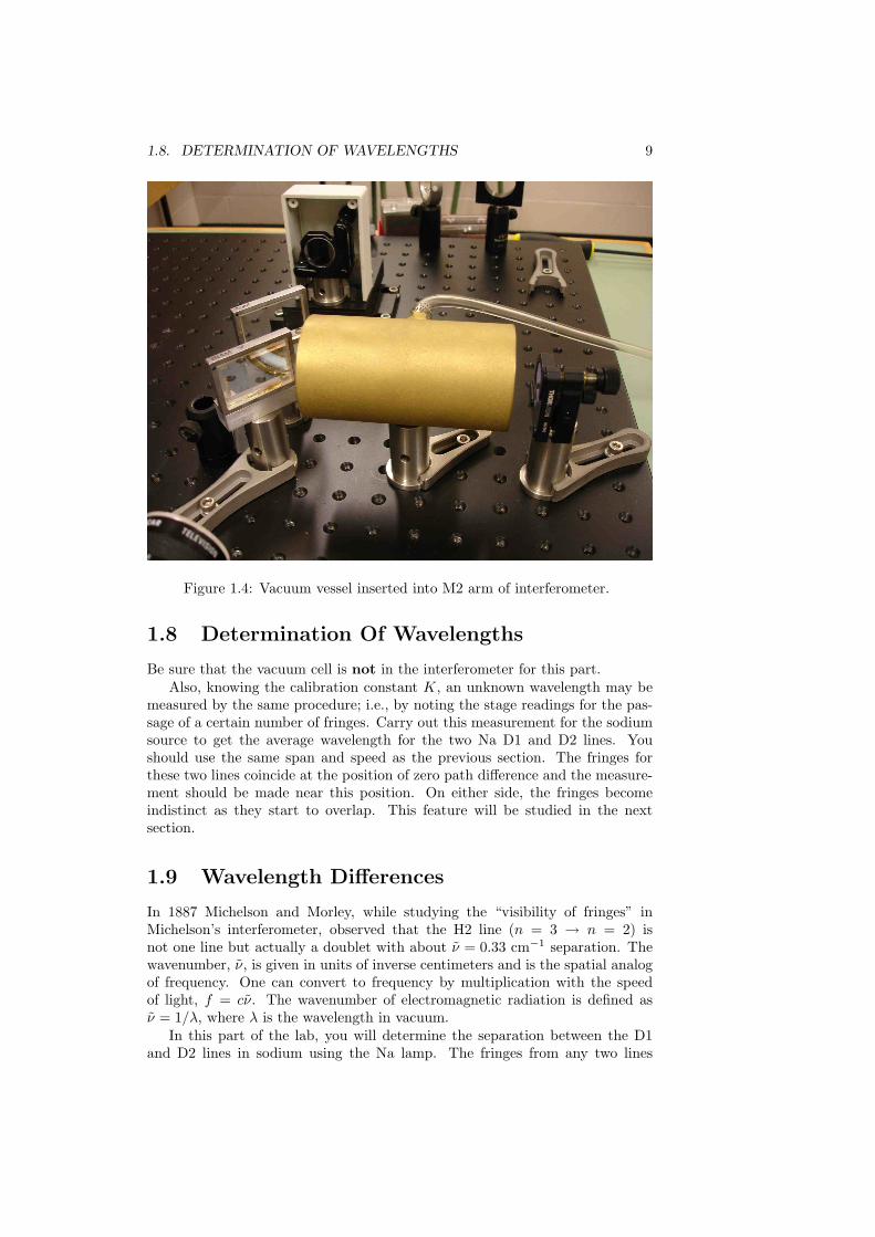
To do your measurement, you should first prepare a vacuum in the cell:close the “leak valve” and open the “pump valve” and turn on the vacuumpump. After the pressure in the cell (as read by the meter) has dropped to theminimum on the scale, close the “pump valve” and turn off the pump. Startthe data acquisition and slowly open the “leak valve” to let in air while youcount fringes. You may need some practice introducing the air fast enough thatthe pressure rises to atmospheric pressure during the time you have set whilenot rising too quickly so that you miss the passage of fringes due to the finitesampling time of the video capture. Be careful to insert the glass vacuum cellwithout hitting or misaligning the mirrors (see Fig. 1.4).

Would you have counted the same number of fringes if you hadused the Na lamp instead of the HeNe laser for this measurement?Why or why not? What is your value for the index of refraction ofair for 632.8 nm light? Does this agree with the “accepted” value?What are your sources of error? Could you use this apparatus as abarometer or thermometer?

1.8. DETERMINATION OF WAVELENGTHS 9

Figure 1.4: Vacuum vessel inserted into M2 arm of interferometer.

1.8 Determination Of Wavelengths

Be sure that the vacuum cell is not in the interferometer for this part.Also, knowing the calibration constant K, an unknown wavelength may be

measured by the same procedure; i.e., by noting the stage readings for the pas-sage of a certain number of fringes. Carry out this measurement for the sodiumsource to get the average wavelength for the two Na D1 and D2 lines. Youshould use the same span and speed as the previous section. The fringes forthese two lines coincide at the position of zero path difference and the measure-ment should be made near this position. On either side, the fringes becomeindistinct as they start to overlap. This feature will be studied in the nextsection.

1.9 Wavelength Differences

In 1887 Michelson and Morley, while studying the “visibility of fringes” inMichelson’s interferometer, observed that the H2 line (n = 3 → n = 2) isnot one line but actually a doublet with about ν̃ = 0.33 cm−1 separation. Thewavenumber, ν̃, is given in units of inverse centimeters and is the spatial analogof frequency. One can convert to frequency by multiplication with the speedof light, f = cν̃. The wavenumber of electromagnetic radiation is defined asν̃ = 1/λ, where λ is the wavelength in vacuum.

In this part of the lab, you will determine the separation between the D1and D2 lines in sodium using the Na lamp. The fringes from any two lines


Vacuum Gauge

M2

“leak valve” “pump valve” pump on/offswitch

Figure 1.5: Vacuum pump, valves, and vacuum gauge for vacuum cell.

(wavelengths λ1 and λ2), such as the Na D1 and D2 lines, always overlap at theposition of zero path difference. If the stage is moved away from this position,either forwards or backwards, then a position will be reached (at a distance d)where the bright fringes of one line fall on the dark fringes of the other. Theresulting fringe pattern is then very indistinct − the fringes are said to have lowvisibility. This particular distance is

2d = (N + 1)λ1 = Nλ2 (λ1 < λ2) (1.3)

where N is an integer. The wavelength difference is, therefore;

∆λ = λ2 − λ1 = 2d(

1N− 1N + 1

)=λ1λ2

2d(1.4)

If λ1 and λ2 differ by very little, it is sufficient to replace their product byλ2, where λ is the average of the two. The expected value of ∆λ ∼0.6nm.

1.9.1 Procedure

Be sure that the vacuum cell is not in the interferometer for this part.Set up a white light source and locate the white light fringes as you did

previously. This will locate the stage at zero path difference. Recall that due tobacklash the stage position will differ if you approach this position from above

1.10. FOURIER TRANSFORM SPECTROSCOPY 11

versus from below. Since you will eventually be using a MATLAB script totake data, and this script moves the stage forward (i.e. to higher values onthe indexed stage), then backwards, then forward again back to the startingpoint, you should always approach from below your position of zero-path lengthdifference.

Replace the white lamp with the sodium lamp. Now move the stage using thetoggle lever on the controller, move the stage over a distance of at least 2 mm not-ing the stage readings at several positions of minimum visibility. When recordingthe positions, you should always move the stage in same direction to avoid back-lash errors. Repeat this process several times and average the stage readings.You can do this manually or you can use the script from before. Your code willagain look like this>> d = michelson_timestream(span, speed);

where you choose span and speed appropriately. A span = 1.0 and speed =0.01 are probably good starting values for this part.

From the average value of ∆D obtained, and the measured calibration con-stant, K, calculate d from equation 1.2, and hence obtain a value for ∆λ fromequation 1.4. Use the average value of the two Na D1 and D2 lines that youdetermined above and find the difference between the two lines.

1.10 Fourier Transform Spectroscopy

So far you have investigated the behavior of the interference fringe pattern asa function of the optical path difference for different optical sources. In generalthe fringe pattern intensity versus the optical path difference (or equivalentlyversus the time delay between the two interfering beams) is related to the powerspectrum of the light entering the amplitude division interferometer by a Fouriertransform. Therefore one can easily measure the optical power spectrum usingthe measurement of the intensity variation as a function of stage position.

Let’s see how this works 1. The electric field incident on the camera is thesum of the electric fields E1 and E2 arriving from M1 and M2 respectively afterhaving passed through the beam splitter. Assuming for the moment that theinput source is a purely monochromatic wave, we can characterize these electricfields with a vector amplitude (encoding the strength and polarization of thewave) and a spatial and time dependent phase:

E1 = A1ei(k1·r−ωt+φ1) (1.5)

E2 = A2ei(k2·r−ωt+φ2). (1.6)

The phase includes terms (φ1 = |k1| l1 and φ2 = |k2| l2) which depend on theoptical path lengths from the beamsplitter along path l1 (encountering M1) andpath l2 (encountering M2). The intensity on the camera is simply the square ofthe total electric field:

I = |E|2 = E ·E∗ = (E1 + E2) · (E∗1 + E∗2) (1.7)= |A1|2 + |A2|2 + 2A1 ·A2 cos θ (1.8)

= I1 + I2 + 2√I1I2 cos θ (1.9)

1This derivation follows that in “Introduction to Modern Optics” by Grant R. Fowles


where we have assumed in the last step that the waves have the same polarizationand that θ = (k1 − k2) · r + φ1 − φ2. You might be wondering about a whitelight source which is probably completely unpolarized. Is this assumption stillvalid in that case? This assumption is justified since the two fields E1 and E2

are copies of the incident field generated by the beam splitter. As long as thebeam splitter and the optics which follow preserve the polarization of the light,these two fields will arrive at the detector with exactly the same polarization(whatever it was at the input of the interferometer). What could the beamsplitter and following optics do to change the polarization of the inputlight?

If the interferometer is well aligned so that the waves are co-linear (k1 = k2)and the 50/50 beamsplitter generates two waves of the same intensity (I1 =I2 = I/2), then the interference pattern is simply

I(x) = I(1 + cos kx) (1.10)

where x = l1 − l2 is the path length difference and k = |k1| = 2π/λ is themagnitude of the wavevector.

Okay, now in general, the light illuminating the interferometer will be com-posed of many different frequencies. So, let’s model the power spectrum of theincident light as a continuous distribution, G(ω). Then the total optical poweremitted into the interferometer in the frequency range from ω0 to ω0 + dω(where dω is an infinitesimally small frequency band) is simply G(ω0)dω. Forconvenience, we can instead use the distribution over wavelength G(k) (whereω = ck). Then the optical power, P , hitting the detector from illuminating theinterferometer with this polychromatic source will be the sum of the interfer-ence patterns from each monochromatic wave composing G(k). Assuming theinterferometer is ideal and has no losses, we have then:

P (x) =∫ ∞

0

G(k) (1 + cos kx) dk (1.11)

=∫ ∞

0

G(k) dk +∫ ∞

0

G(k)eikx + e−ikx

2dk (1.12)

=12P (0) +

12

∫ ∞−∞

G(k)eikx dk (1.13)

where P (0) is simply the power measured at zero path length difference. Wecan rearrange this expression and define the power function W (x)

W (x) = 2P (x)− P (0) =∫ ∞−∞

G(k)eikx dk. (1.14)

We see then that the power function W (x) is the inverse Fourier transform ofthe power spectral density G(k). Inverting this expression we have that thepower spectrum is the Fourier transform of the power function

G(k) =1

2π

∫ ∞−∞

W (x)e−ikx dx, (1.15)

or equivalently

G(ν) =1

2π

∫ ∞−∞

W (x)e−i2πνx/c dx. (1.16)


Monochromatic

(laser)

Two wavelengths

close together

(NaD lamp)

Wide band-pass

filter

(white light)

Narrow band-

pass filter

(orange filter)

mirror position

coherence length

Figure 1.6: Fringe patterns plotted as a function of the mirror position. Noticehow the fringe visibility collapses and then revives as a function of the mirrorposition when the spectrum is discrete. Also, note that if the mirror is moved adistance d, the optical path length between the two arms in the interferometerchange by 2d.

1.10.1 Procedure

Be sure that the vacuum cell is not in the interferometer for this part.In this stage of the experiment, you will use the interferometer to realize


a Fourier transform spectrometer. The idea is to translate the stage aroundthe zero path length position (ZPL), record the fringe pattern, and use it todetermine the power function W (x) and then compute numerically the corre-sponding spectral density G(k) of various optical sources. To do this, you will(as before) use the MATLAB script “michelson timestream.m” which recordsan array of power values for each video frame (i.e. each stage position). You willuse your calibration constant for the motion, K, to deduce the stage position ateach frame and therefore generate the power function W (x) (be sure the stagevelocities are set the same or else recalibrate K for this part). From this you willnumerically compute the Fourier transform to determine the power spectrum ofthe light.

wavelength (nm)

pow

er (

arb. u

nits)

White Light

200 300 400 500 600 700 800 900 1000

10

20

30

40

50

60

Figure 1.7: Example spectrum from the incandescent bulb measured by theMichelson Fourier transform spectrometer. Your reference white light spectrumshould look something like this one. Keep in mind that this measurement ofthe spectrum is ultimately limited by the wavelength dependent transmissionof the optical elements in the Michelson interferometer and by the sensitivityof the CCD detector. See Fig. 1.8 for a typical response curve of a silicon CCDimage sensor.

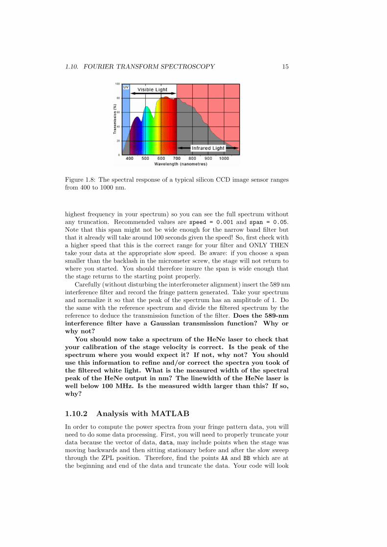
As before, set up a white-light source, find the fringes at zero path lengthdifference, make them vertical, and note the stage setting. Before taking eachdata run, you should carefully adjust the iris on the camera lens to maximizethe fringe brightness without saturating the camera. This will optimize thesignal to noise and produce much better data. Start by recording the fringepattern and computing the spectrum of the white light source. You should geta spectrum similar to that shown in Fig. 1.7. This is your reference spectrumwhich you will be modifying with a filter. Keep in mind that this measurementof the white light source spectrum is ultimately limited by the transmission ofthe optical elements in the Michelson interferometer and by the sensitivity ofthe CCD detector. See Fig. 1.8 for a typical response curve of a silicon CCDimage sensor.

To take the data for this section, you will again be using the MATLABscript “michelson timestream.m”, only this time, you should use a very slowspeed and a very narrow span since the filtered white light has a short coher-ence length and you will need good spatial resolution (which will determine the


Figure 1.8: The spectral response of a typical silicon CCD image sensor rangesfrom 400 to 1000 nm.

highest frequency in your spectrum) so you can see the full spectrum withoutany truncation. Recommended values are speed = 0.001 and span = 0.05.Note that this span might not be wide enough for the narrow band filter butthat it already will take around 100 seconds given the speed! So, first check witha higher speed that this is the correct range for your filter and ONLY THENtake your data at the appropriate slow speed. Be aware: if you choose a spansmaller than the backlash in the micrometer screw, the stage will not return towhere you started. You should therefore insure the span is wide enough thatthe stage returns to the starting point properly.

Carefully (without disturbing the interferometer alignment) insert the 589 nminterference filter and record the fringe pattern generated. Take your spectrumand normalize it so that the peak of the spectrum has an amplitude of 1. Dothe same with the reference spectrum and divide the filtered spectrum by thereference to deduce the transmission function of the filter. Does the 589-nminterference filter have a Gaussian transmission function? Why orwhy not?

You should now take a spectrum of the HeNe laser to check thatyour calibration of the stage velocity is correct. Is the peak of thespectrum where you would expect it? If not, why not? You shoulduse this information to refine and/or correct the spectra you took ofthe filtered white light. What is the measured width of the spectralpeak of the HeNe output in nm? The linewidth of the HeNe laser iswell below 100 MHz. Is the measured width larger than this? If so,why?

1.10.2 Analysis with MATLAB

In order to compute the power spectra from your fringe pattern data, you willneed to do some data processing. First, you will need to properly truncate yourdata because the vector of data, data, may include points when the stage wasmoving backwards and then sitting stationary before and after the slow sweepthrough the ZPL position. Therefore, find the points AA and BB which are atthe beginning and end of the data and truncate the data. Your code will look


something like the following:

>> rawdata = michelson_timestream(span, speed);>> data = rawdata(AA:BB);

Inspect a plot of your data to check that it has been properly truncated. Now,you should transform your vector of data into something equivalent to W (x)(well equivalent up to a constant and a scale factor) by subtracting off the meanand then normalizing the data vector with

>> ndata = data-mean(data);>> ndata = ndata/(max(ndata));

Now, to take the Fourier transform, you will use the “Fast Fourier Transform”function (fft) which, because of the structure of this super-efficient numericalalgorithm, requires that you feed it a vector whose length is equal to a powerof 2. Fortunately you can feed the function your vector and tell it the lengthis longer by rounding up to the next higher power of 2 (and the function willautomatically pad your data with zeros at the end to fill in the gap). for this,use some code like the following:

>> L = length(ndata);>> NFFT = 2^nextpow2(L);>> fftdata = abs(fftshift(fft(ndata,NFFT)));>> fftdata_oneside = fftdata(NFFT/2+2:NFFT);>> nfftdata_oneside = fftdata_oneside/max(fftdata_oneside);

This will give you the absolute value of the Fourier transform since we aren’tinterested in the phase factors, only the amplitude versus wavelength. Also,we are only interested in the positive frequency components of the FT, so wewill plot fftdata_oneside. The last line just normalizes the result by themax value. Why are the array limits NFFT/2+2 and NFFT for the command“>> fftdata_oneside = fftdata(NFFT/2+2:NFFT);”? The reason is that the(N/2+1) element is the zero frequency bin and the (N/2) element is actuallyone of the negative frequency bins. The positive frequencies start at (N/2 + 2).

Now, the data contained in fftdata are the values of |G(k)| (technically|Gn| since we just have a list of values indexed by n) where the sample sizeis ∆k = 2π

Ns∆x. Ns = NFFT is the number of samples in the data which was

“Fast Fourier Transformed” and ∆x is the step size in, for example, nanometersbetween images. Remember since ∆x is defined as the amount the optical pathlength varied between frames, it is twice the amount the carriage moved betweenimages.

So, you know that each value of |Gn| is paired with a wavevector of k =n×∆k. But you should plot your spectral data in terms of wavelength |G(λ)|and so you need to create a vector of λ values corresponding to each point in|Gn|. Using the fact that k = 2π

λ , we can write that λ = 2πn∆k

>> n=1:1:NFFT/2-1;>> lambda=zeros(size(fftdata_oneside));>> lambda=NFFT*delta_x./n;


>> plot(lambda,fftdata_oneside);

The little dot (.) at the end of delta_x. insures that the division to create thevector lambda from the vector n happens element-wise.

An alternative and more transparent example is the following (given yourdata file has an EVEN number of elements):

>> data = rawdata(AA:BB);>> data = data - mean(data);>> N = length(data);>> spec = abs(fft(data));

Now we remove (or just leave out) the zero frequency at index 1, and ’negative’frequencies (N/2+2:N)...

>> spec = spec(2:N/2+1);>> spec = spec / max(spec);

And, since we’ve removed zero frequency, the lambda index starts at 1.

>> n = 1:N/2;>> lambda = N*delta_x./n;>> plot(lambda, spec);

The Michelson Interferometer - CWSEI · The Michelson Interferometer ... Using the WinTV2000...

Documents

Transcript of The Michelson Interferometer - CWSEI · The Michelson Interferometer ... Using the WinTV2000...