The Method of Expected Number of Deaths, 1786-1886-1986 ... · Method of Expected Number of Deaths,...

The Method of Expected Number of Deaths, 1786-1886-1986, Correspondent PaperAuthor(s): Niels KeidingSource: International Statistical Review / Revue Internationale de Statistique, Vol. 55, No. 1(Apr., 1987), pp. 1-20Published by: International Statistical Institute (ISI)Stable URL: http://www.jstor.org/stable/1403267 .

Accessed: 19/11/2013 08:27

Your use of the JSTOR archive indicates your acceptance of the Terms & Conditions of Use, available at .http://www.jstor.org/page/info/about/policies/terms.jsp

.JSTOR is a not-for-profit service that helps scholars, researchers, and students discover, use, and build upon a wide range ofcontent in a trusted digital archive. We use information technology and tools to increase productivity and facilitate new formsof scholarship. For more information about JSTOR, please contact [email protected].

.

International Statistical Institute (ISI) is collaborating with JSTOR to digitize, preserve and extend access toInternational Statistical Review / Revue Internationale de Statistique.

http://www.jstor.org

This content downloaded from 132.216.65.156 on Tue, 19 Nov 2013 08:27:17 AMAll use subject to JSTOR Terms and Conditions

http://www.jstor.org/action/showPublisher?publisherCode=isi

http://www.jstor.org/stable/1403267?origin=JSTOR-pdf

http://www.jstor.org/page/info/about/policies/terms.jsp


International Statistical Review (1987), 55, 1, pp. 1-20. Printed in Great Britain

? International Statistical Institute

Correspondent paper

The Method of Expected Number of

Deaths, 1786-1886-1986 Niels Keiding Statistical Research Unit, University of Copenhagen, Blegdamsvej 3, DK-2200 Copenhagen N, Denmark

Summary

The method of expected number of deaths is an integral part of standardization of vital rates, which is one of the oldest statistical techniques. The expected number of deaths was calculated in 18th century actuarial mathematics (Dale, 1777; Tetens, 1786) but the method seems to have been forgotten, and was reinvented in connection with 19th century studies of geographical and occupational variations of mortality (Neison, 1844; Farr, 1859; Westergaard, 1882; Rubin & Westergaard, 1886). It is noted that standardization of rates is intimately connected to the study of relative mortality, and a short description of very recent developments in the methodology of that area is included.

Key words: Cox regression; Dale, W.; Epidemiology; Farr; Generalized linear models; Neison; Occupational mortality; Poisson assumption in epidemiology; Price, R.; Proportional hazards; Relative mortality; SMR; Standardization; Tetens; Westergaard; Yule.

1 Introduction

Current texts on standardization of vital rates often emphasize the rather deep historical roots of that subject; see, for example, Benjamin (1968, p. 97), Lilienfeld (1978), Logan (1982, p. 9) or Inskip, Beral & Fraser (1983). Often Farr (1859), or occasionally Neison (1844), see Lilienfeld (1978), is credited with the first use of the concept and, as we shall see below, these authors were admirably clear in explaining the background for and methodology of standardization. However, analogous calculations of expected numbers of deaths were used in the 18th century literature on actuarial mathematics. We shall in the present paper describe the calculations by Dale (1777) and Tetens (1786). Dale may very well be the earliest to explain and use the method (which he did in full detail). Tetens demonstrated the calculation (including corrections due to loss to follow-up) and also suggested what we would today call parametric statistical models for excess (or relative) mortality.

Standardization of rates was later primarily used in official statistical publications, where considerations on random errors due to sampling were (and often still are) stated verbally at the most. It seems to be generally accepted that Yule (1934) was the first to derive the standard error of standardized rates. However, Westergaard (1882) gave a rather careful discussion of sampling errors of mortality (and morbidity) statistics. The occupational mortality study by Rubin & Westergaard (1886), to be presented here, is an early application of standardization as an analytical-statistical methodology.

Only rather recently have the concept of standardization and the method of expected numbers of death been put into full theoretical-statistical perspective. We review and



2 N. KEIDING

slightly extend the discussions by Berry (1983) of calculating expected mortality, and by Breslow (1975), Breslow & Day (1975, 1985) and Hoem (1987) of interpreting the standardized mortality ratio as a maximum likelihood estimator in a proportional hazards model.

Generalizations to regression models with continuous time and continuous covariates were developed and surveyed by Breslow et al. (1983), Andersen et al. (1985) and Breslow & Langholz (1986). We shall conclude this presentation by a brief reference to their work.

2 Brief review of standardization

In the simplest setting, standardization is concerned with k age groups, where a standard population with s, individuals in the first group,... , Sk in the kth, in short, age distribution s,, .. , sk, and age (-group)-specific death rates A,--... , Ak, is compared to a study population with age distribution a1, ... , ak and death rates cx, ..., tak. This means that the number of deaths in the standard (study) population is E siA (E aicri).

The expected number of deaths in the study population if the standard death rates are applied to it is E aAi,, and a comparison of this with the actual number of deaths in the study population is said to be 'corrected' for the dependence of mortality on age. This comparison is often made in terms of the standardized mortality ratio

S aoai, actual no. deaths in study population

SMR -

E aiA, expected no. deaths in study population'

usually this is multiplied by 100. An important property of the SMR is that it may be calculated on the basis of the total number of deaths only, without knowledge of the age distribution of the dead.

Alternatively one might compare the actual number of deaths in the standard population with that expected if the study population death rates are applied to the standard population. This yields the comparative mortality figure, or standardized rate

ratiosi CMF = SRR = ( x 100)

and because this may be interpreted directly as a ratio of weighted means of the age-specific death rates to be compared, (using the (relative) standard age distribution as weights), the method is called direct standardization. The weights are the same for all study populations that one might want to consider.

The SMR may be interpreted similarly, although somewhat less directly, namely by using the weights

ai A Esii

That these are more complicated seems to be the basis for terming the corresponding method of standardization 'indirect'.

3 London in the 1770s: Careless societies for the benefit of old age, Richard Price and William Dale

Around 1770 many societies were formed in London with the purpose of providing annuities for the members and/or their widows. Almost all of these were however based on quite insufficient plans, and Richard Price (who is now perhaps better known as the publisher of Bayes's essay and as the 'ethical father of the American revolution')



Method of Expected Number of Deaths, 1786-1886-1986 3

published his treatise Observations on Reversionary Payments (Price, 1771) with the explicit purpose of demonstrating the inadequacy of most of these plans. In Price's own words in a letter to George Walker, August 3, 1771 (quoted from Price (1983, p. 102)):

The Treatise I have lately published has gone off better than I expected. The London Societies are in general alarmed. I wish I may prove the means of either breaking them, or engaging them to reform. They have in their present state a very pernicious tendency.

The next year another book (Dale, 1772) appeared with the same purpose but using more elementary mathematics and containing a detailed review of each of 11 societies. (This book was, formally anonymously, published by 'a fellow of one of the societies'.)

William Dale had however little luck in reforming the Laudable Society of Annuitants (which he belonged to) so, after having resigned, he published in 1777 (again formally anonymously) a 'Supplement' (Dale, 1777).containing further detailed demonstrations of the inadequacy of the plan of the society. Dale provided a very detailed and polemic account of his debate with the society, but we shall here concentrate on his calculation of expected mortality. In his own words (p. 6): The real Mortality for seven years past in the LAUDABLE SOCIETY, has been compared with the expected Mortality by Dr. Halley's Table; the particulars are hereto annexed, (at p. 60) which will shew that but few more than HALF SO many have hitherto died in the Society, as BRESLAW Mortality supposed would die.

Dale goes on to point out that

It may be well presumed that the healthiest, such as have an opinion of the strength of their own constitution, so as to expect to live to enjoy the annuity, would engage in the Laudable Society of Annuitants, and that the opposite may be presumed for (the husbands) joining the Laudable Society for benefit of Widows.

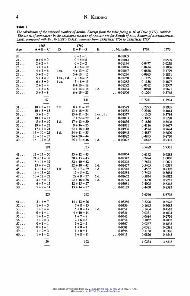
The calculation is explained in 'Section XIII, Of Mortality, real and expected, in the Society'. The calculations are set out in a large fold-out table, where the annual increments, decrements and one-year agings are given for one-year age classes for all the years involved; see Table 1 and Plate 1.

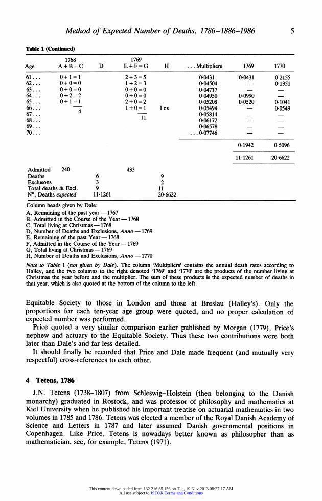
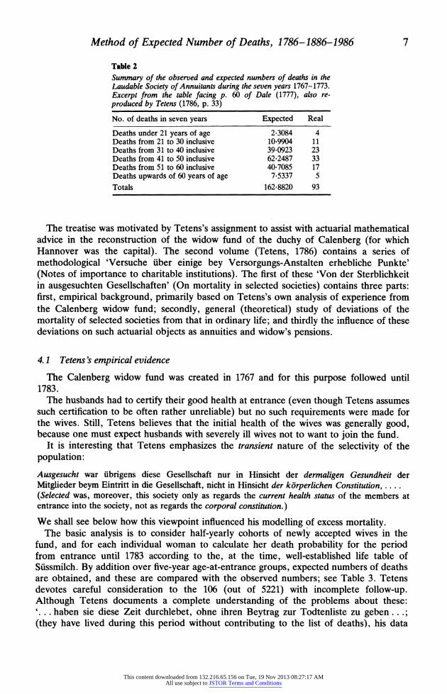
A curious point is that Dale, being only concerned with demonstrating that the expected mortality is far higher than the observed, biases his calculations deliberately in the following two ways: he disregards mortality in the year of entrance into the society, and he consistently deletes decimals (rather than rounding) in the calculations of expected number of deaths. Dale summarizes his calculations for the first seven years in a small table, here given as Table 2, and corresponding in modern terminology to SMR= 93/163 x 100 = 57.

Until further evidence may surface, it seems fair to claim that Dale was the first to carry through a detailed calculation of the expected number of deaths. In fact, his table and explanation could still be used as a thorough introduction to standardization.

Dale (1772) reproduces an application that he submitted on September 24, 1771 for the vacant position of Secretary to the Provident Society (he did not get the job, his analysis of the society being considered unintelligible containing, as it did, decimals, etc.). He here introduced himself as 'a person in his 46th year of age, who lately lived with a nobleman as house steward'. Elsewhere, Dale (1772, preface) emphasizes that he is without 'the advantage of a liberal education'. The books allow no other interpretation than being entirely Dale's own enterprise, done out of interest in correcting the insufficient plans of the 'Societies'.

Price's treatise was reprinted several times. In the fourth edition Price (1783) included a brief comparison of the rates of mortality (in ten-year age groups) of the members of the



4 N. KEIDING

Table 1 The calculation of the expected number of deaths. Excerpt from the table facing p. 60 of Dale (1777), entitled: 'The STATE of MORTALITY in the LAUDABLE SOCIETY Of ANNUITANTS for Benefit of AGE, Bottom of BARTHOLOMEW- LANE, compared with Dr. HALLEY'S TABLE, annually from CHRISTMAS 1766 to CHRISTMAS 1775'

1768 1769 Age A+B=C D E+F=G H ... Multipliers 1769 1770

20... 0+1=1 ...0-01003 21... 0+0=0 0 + 5 = 5 0-01013 - 0-0505 22... 2 + 2 = 4 0 + 2 = 2 0-01194 0-0477 0*0238 23... 3 + 1 = 4 4+6= 10 0-01036 0*0414 0-1036 24 ... 4 + 2 = 6 1 ex. 4 + 13 = 17 0.01047 0.0628 0-1779 25 ... 5 + 2 = 7 5 + 10 = 15 0.01234 0-0863 0-1851 26... 5 + 4 = 9 1 ex., 1 d. 7 + 8 = 15 0.01250 0.1125 0-1875 27... 6 + 3 = 9 1 ex. 7 + 8 = 15 0.01265 0-1138 0-1897 28 ... 2 + 2 = 4 8 + 10 = 18 0.01282 0*0512 0.2307 29 ... 1 + 5 = 6 4 + 14 = 18 1 d. 0.01484 0.0890 0-2671 30... 3 + 5 = 8 6 + 19 = 25 .. .0.01506 0-1204 0-3765

57 141 0-7251 1.7924

31 ... 10 + 5 = 15 2 d. 8 + 11 = 19 0.01529 0-2293 0-2905 32 ... 10 + 3 = 13 13 + 18 = 31 0.01553 0-2018 0-4814 33... 5 + 2= 7 13 + 11= 24 1 ex., 1 d. 0.01577 0-1103 0-3784 34 ... 10 + 7 = 17 7 + 22 = 29 1 d. 0-01803 0-3065 0-5228 35 ... 5 + 5 = 10 1 d. 17 + 13 = 30 0.01836 0-1836 0.5508 36 ... 19 + 3 = 22 9 + 16 = 25 0.01871 0.4116 0-4677 37 ... 17 + 7 = 24 22 + 18 = 40 0.01906 0.4574 0.7624 38 ... 15 + 10 = 25 1 d. 24 + 11 = 35 0.01943 0-4857 0-6800 39 ... 10 + 15 = 25 24 + 20 = 44 0*01982 0.4955 0-8720 40 ... 16 + 17 = 33 25 + 21 = 46 1 d. ... 0.02022 0.6672 0-9301

191 323 3.5489 5-9361

41 ... 13 + 17 = 30 33 + 12 = 45 0.02064 0-6192 0-9288 42 ... 21 + 11 = 32 30 + 13 = 43 0.02342 0-7494 1-0070 43 ... 18 + 14 = 32 32 + 10 = 42 0.02398 0-7673 1-0071 44 ... 13 + 9 = 22 32 + 10 = 42 1 d. 0.02457 0-5405 1-0319 45 ... 4 + 14 = 18 1 d. 22 + 7 = 29 1 d. 0.02518 0.4532 0.7302 46... 14 + 15 = 29 17 + 5 = 22 0.02584 0-7493 0.5684 47 ... 10 + 12 = 22 29 + 8 = 37 1 d. 0*02652 0-5834 0-9812 48 ... 4 + 8 = 12 22 + 16 = 38 1 d. 0.02724 0-3268 0-9261 49... 6 + 7 = 13 12 + 15 = 27 0.03081 0-4005 0-8318 50 ... 5 + 9 = 14 13 + 14 = 27 . .. 0-03179 0.4450 0-8583

224 352 5-6346 8-8708

51 ... 3 + 4 = 7 14 + 12 = 26 0.03280 0.2296 0-8528 52... 1 + 4 = 5 7 + 8 = 15 0.0339 0-1695 0-5085 53... 1 + 3 = 4 5 + 8 = 13 1 d. 0.0351 0.1404 0-4563 54 ... 0 + 1 = 1 4 + 10 = 14 0.0331 0.0331 0.4634 55... 1 + 1 = 2 1 + 7 = 8 0.0342 0*0684 0.2736 56... 1 + 2 = 3 2 + 6 = 8 0.0354 0-1062 0-2832 57... 0 + 1= 1 3 + 2= 5 0*0367 0*0367 0-1835 58... 0 + 1= 1 1 + 0 = 1 0.0381 0-0381 0-0381 59... 1 + 2= 3 1 + 0 = 1 0.0396 0.1188 0-0396 60... 1 + 1 = 2 3+8=11 .. . 0.0413 0*0826 0.4543

29 102 1-0234 3-5533




Table 1 (Continued)

1768 1769 Age A+B=C D E+F=G H ... Multipliers 1769 1770

61... 0 + 1= 1 2 + 3 = 5 0*0431 0-0431 0-2155 62... 0+0=0 1 + 2 = 3 0*04504 - 0-1351 63... 0+0=0 0+0=0 0-04717 - - 64... 0+2= 2 0+0= 0 0-04950 0.0990 65... 0 + 1 = 1 2+0=2 0*05208 0*0520 0-1041 66... 1 + 0 =1 1 ex. 0*05494 - 0.0549 67... 4 0*05814 - - 68... 11 0*06172 - - 69... 0*06578 - - 70 ... ... 007746 - -

0.1942 0.5096

11-1261 20-6622

Admitted 240 433 Deaths 6 9 Exclusons 3 2 Total deaths & Excl. 9 11 No, Deaths expected 11-1261 20-6622

Column heads given by Dale: A, Remaining of the past year - 1767 B, Admitted in the Course of the Year - 1768 C, Total living at Christmas - 1768 D, Number of Deaths and Exclusions, Anno - 1769 E, Remaining of the past Year - 1768 F, Admitted in the Course of the Year - 1769 G, Total living at Christmas - 1769 H, Number of Deaths and Exclusions, Anno - 1770

Note to Table 1 (not given by Dale). The column 'Multipliers' contains the annual death rates according to Halley, and the two columns to the right denoted '1769' and '1770' are the products of the number living at Christmas the year before and the multiplier. The sum of these products is the expected number of deaths in that year, which is also quoted at the bottom of the column to the left.

Equitable Society to those in London and those at Breslau (Halley's). Only the proportions for each ten-year age group were quoted, and no proper calculation of expected number was performed.

Price quoted a very similar comparison earlier published by Morgan (1779), Price's nephew and actuary to the Equitable Society. Thus these two contributions were both later than Dale's and far less detailed.

It should finally be recorded that Price and Dale made frequent (and mutually very respectful) cross-references to each other.

4 Tetens, 1786

J.N. Tetens (1738-1807) from Schleswig-Holstein (then belonging to the Danish monarchy) graduated in Rostock, and was professor of philosophy and mathematics at Kiel University when he published his important treatise on actuarial mathematics in two volumes in 1785 and 1786. Tetens was elected a member of the Royal Danish Academy of Science and Letters in 1787 and later assumed Danish governmental positions in Copenhagen. Like Price, Tetens is nowadays better known as philosopher than as mathematician, see, for example, Tetens (1971).



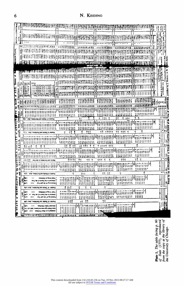
Plate 1. The table facing p. 60 of Dale (1777), reproduced from the copy at the library of the University of Chicago.

TV-nSTATEWMURTILITY

in the LAKUDABLEOCIETYof ANNUIT MEW- ANo ADEATH*.a

CHRISTMA.

rewith Dr. HALLEY's TABLE, annuall f APm Ci 7667t C4-T17 75 111 6 1769.

-

n ? I 713 4. tow no 0" - ftwl

JI 1768. ' r r1771. 177L. 737.- ~~'4; *

-99Y OS~ = 0 ;7, 0o+ 2= 3 1 Its =+. ft 0+ Q ~ + = 0 114 6 + c 0 0+ = I .I+O=IId. ++= 0= a 0+O a .06

o66 0+1=a_+ = 1 .+ O= 1 .f

9o476! .0476 1; .333

+ O= 081 + O= 1 1 O=*

1 4 -038

-P

+.=t Id-1+1=41:. -5 I c= + ;e. O 0 .oo 009o .2

i '

iii i"• ! "6 ,I.~ .7

, .s68 ~ ~

O ? d

+= 0 + O= a 0 + O +0= 0 += 1 += 0 U .A5 .0-z 5 9 6"X59 .759

+ 0+ O=0 O=0 0+ -=

0 8 ++= 44 4

. 4+ 4 +040; I

9 .

L* .094

-_._7 I O= a+ X+ I + 0+ 1=100= + 1= + 0+ O= 0 1 - -14 .5 . 5 4

30 -c+

A +

I+4 *a ~ ~ 6 o6 += 707~ .o ot ..013 ~ ~ *4 6 -01 ~34 [' 013+ ~s

++1 0++Ot o +2+ +=3 2 ad. +0= 1+0= 1 94 *0 43 No Is .0131 .058-921 WI + I + O= 0) + Q= 0 24 2+O=3 +O=Ito .021 -24 .4

o+ O + + 1 + I = 0 1 & + 0=@13 6+ j O =0 06 i O aI .t.01073 .021 107 4- o 5 ,1

Is I j I L 1 .1111 .0181 185 .0093 --1 12 -053 +7 a 0++ 1 + 1 + . = + O+ ad +o o= 1 I0+ O= a I a .070

%0*O's .0- 05541*:05

?+ 0= 3+1= 4ex I +O= 1

| + *= 1o+O 1 .1 -0-37 3.0 7 09 1 .0 7047

g4 6 4+~a8 + ;

v+ 0= 0 =2 O ='d S I +7O==17 2+1O=7 A 14 -00946 . a 9.a Z" 6 -0"4 989.-"4 '01S9 .03773

1 14 7 ..

.5=1

o8 .44.

+ .4 7 .01931 CO3

ae + 3 + O=1 0+ O= 9 + O= 2 1 + O= is 9;1 '95 05.11!

ago Is *6 a7 .

09 6 .04 95"l- 1'7

3.+r I 1+ 0= 3 1Z 3+ O= 13 0+ :+ O=S2 1 000 A V4

17 0 5 ~ +.=4. 1 ; ~ 943 01 + 4= 4 +10=131*O= I J Se .37 ~ . 5389 .09;291! .0097 j,1 .00-'s

,.

3+ = 1.O0

0

S+ 4 + 4= +4 r 3+ O= 4 1 +0 = . .9 .6 .t .3+I .1+ O= I *s .098 X e . 03 9

Z I9

3 3 = + 0 + o=1 907.3 06 .0 09 7.4

7

,

, 7

z

+ 4 = 3+O= 4 3+ O=4 4

O+

43 9 04 37 *S .' .4 .6z am o70 19

go

8 7

4.3$6

X +4=4 + 7= 3 4 4+ + *+ a 4 + O 46 1+ =O= I so .040.3 t -04.6 . 09409~ .3047 1! .-01 0i 4.160tiL_ .1,04

,@,=5 8+0 ~ 3154 4 7

,=~ 37.913+

=5 +3493 091 .37

44

.7 ., 88

9l

q 7-4__

d +jq , = .i =? +3 z769675

.5~ .90 ~l 8

7.7C S7 6 i !162.176 ., 7 7 ., 511

'8 -446, -326, 2-0841

a6.j#,

0+ 0= +'I+ = 4 4+2= 6- 4 O =6 4 4+ 04 O 4 74+ O= to .01034 . 0 40 - 00 5*- .050 55

a .040 3410 4043030

d. I= 9 S+ I= 4 + I=3 8.5+$i=s 6 5+ 4 6 + c 6 5=7 4 + 1= 5 2 .0114 13 58 . -04767 -013b *-1313 .07 t 1 .00347jl05*C 4 .l7. 3

:0 -015 07351 -5041 7 "0/ 1

14 3~1_.____ 4.7.4

115, 4 g + =12 6+ o 6 4 A*-2oq

J + 47 4+6=10 + 4=6 + 1=+ 7 7+3O= 7323 -01036 -0414+-0414 -103 o1zj I

'ex.

. 10 37 ~ .~U 57 .

4.07|4

*4' 5 '+4a=5 +11=7+55 o6+ 9=19 6+ 2= 1 1 e.I+ s=i4 I. 6+ .jo= ad.7+ O= ;7 24 -01.47 32j 6s? 77. 1989 5 O I I sI odosi'7J 41 A$

A = 7 5+10=15 7+7=2 1+ t=20 Iex 3+ X=49 3+3O=4j 6 + o=3 If 53 1X34 52 1 47 o$63 .q I46 goo 604 -0,,74125 1t74! 8221

AI S+ 5=

7 +31 1 +6=1 2+4=5 +1 =a + O4= 1AIM 7 5 01 .a01 .1 87 -6H 3i 3 1 I0 b $5 5 C26

q' + 4 ex

+ 7$=:I 45+6x=2 Id. so+ a=sO

2ex. + .

0 d I

=2a id + --0975o* , ,.g6 .1 4 t65 z j .5Jogs 5 .47815

1 1 - +3= 9*11 IA .so + =20= S a O= Id.7 oisi +3=40 . 33 9 - 1.3S6 9931 .414 X3 1 2742.10 1.;25

O= 2 1=3 .2 4+ I=2+*o O=1t o s d + .011 .W- 35136 .330-, .-3 .43 5g- co -,. .3205 118 CA.4S a= S *+ 0= t 4 J9I d.s6+ t' s7. 2j.487

2 9+8 +- ; I +4 t4+1 1d IS 4= z A d 2+ 0= 7

d + 1= 17 S= . .03 0 8" .2 6131 .356, 337 i 2 171 4S 7047

I + =5 = + = 8+ 6=4 = e+x= 12+ +o'8 9-0+0 44 .0496 .4 3 .3715 3 .7 soo

S o+- 1 3+3+8 l+ I

=6 o 2+1=54 1C+L24 1=11 61 16 .4363 - -2 5601la

17+2 '+j=; ,j+i= , I5=.2 3 .8 + 41 ad. 7+2=29 17+ 0=17 I30 *433 - *1312 .31 i. 6 j .19 2.349

44 7 + 1 1-3 -,+37 170=ISOd1$7 +012 -559 -72;1 7 a p5 2.fi .'@?4 .49 1 ' 1-9904 1.04S7

1*+5= I+i= i 35+ 4231 + 2=b ,;,At a+ 1=24 41+ a 49 I u- 9+ -1 1 1.12 . 1525 -289 .290S34494 .. -.*

*+=1= + *4 I' +I=,

Id. +0=310 +1 '20 8+ -4 +11 4-4 - 559 4815 5 7 .3 77.2953 2 so+ 3=13 :3 :!=Jl '39"+ I I J; Id- A+ 3= t6 9+ 1=S 2+ O=4 4*9+0 1 1 0530 .&

*+ J= J+ 1 =24 + 39+4=33 381+O= 4 a41 + 0= 27 7+ =15 77 - .03 7 . 614 S -5 7 * ;6s,, '34 6$ . 3, 31.4 to + 7=1-, 7 2 2= 29 312 1=33 I + 0=9 4 - 3+ 5 = 1 AS+ 10=29 + O= 2 34 -o j :901 : os .338 :594 *73 is$ 04 4 a 3-392 40

is I ex. 19ri~p + 3= 3 9 := S so =9 I a 4 1 d.36+ =11 1CL J+ 1 =39 6+ 0=36 3( .33 7 4136 -#77 :729 .42, ? -7-911 -6735 3 +209 441 I _ _45 25 1 + 1* --- if I d+)+5 =0 . -7+ = 4 .381469 .-6

+ 7+=4 IA+ =8= *0I+ 0+04=01 3 =7 - - -+=4 .0 6 .7a 02 4 371 40, 5376

9 : ,'S5

2 00 5 84 IA. 4 4= 3+05=0 + 3=4 +=4 .0 7 -4 95 5 87 -V3 01 $51

- 11 16+17=3 3 5+ 2 1=il I d 44+ 1 =9 43+ N 1 2 . SI+ 6 57 4+ 3=4 1 1+ 3 =4 40 OSO2 6.1 .66s .4io 1-9291-31 85 40 3 h.08 1 if+ 11 11 117 3 jl+1=45 4+ 7=53 AI d. 59+ 4= 5 Io.4+ C=48 57+ 0=57 A+ '43 4 .*S64 -43 . 6egs .938b 1.713 1-300 1704 C75 9 3 6.5s 7409

=1 3+0*o j 0 * 13 =44 =5 + 1 *=63 48+ O= 48 . +0=7 .0127 I- - 13- 47 34 756 9

41 1 A. I+ 4= S 3O=4 4+ 0=4 of, + =53 53+ 1=5 aof6+ 1A4 + 1=4 43 .0 1)98 763 0 1 1 754 15 04 7-17 .

+ I+q=* 3 + 10=4s I*6 i d. 42+ 3=45 + 0=#s s+ 0=5I ex s+ I 5+I d 4+ o=6444 -147 128 -50 3oj1 o0iii 1.31 5 &-26 574 4 4 ,41! -94

I.

1+ 5.1 4+L 4 A = + 4 54 4 Spa 5. s +- J.32109 -31 .25 " 3.345 94 *0.81 '97S:4

*" -~ - 1 ~ -oa ,-m 61,81 Li..g-... m- UCt

7+ 3 1 1+ 5= 17 ( a so+D=Y41

1=4 I d. 0 I 1+ = +7* 46 cs6-5-7 3 58.-2 46 3- 58 11 .

I*+ I Sl x Xq+ 8=37 I d' A+ 5=17 31+ 1=34 43+ 1 =44 1 4. 4+ 2 =4S . + 0=41 4 -4 5 .160 4 .*1 :760 .1 i 47 A 5646,1 6119s J+ S= I* + 16=38 IIA-. )6+ 8=44 5 1. 34+ O= 1.* 1+ 0=43 1S.- ,- + 0 =45 411 AS7* .16 34 7.3a?. 3j7 l5g$a

- 10774

+ + -7

1 T w A E=1N d

C L ONS us j)U by . R LE v j S

0s 3+Ii=27 37('" + S=Jq 43*0=43 d. s6+ o= +=4 I + 04249 .0381 IS0 -00 .31 1.01 4 3 67 49 2 5711 2 J+ I= 1 4: is+Id I~l 1 'f i =H d + ~ 0=.

S+ 4= 7 *6 9 41- 4 + U Ir. ==: dl+O I . O= $6 1 Iiiitso .032 A 096 .115311 1-4104 49 7+ #=Is 4. 3; ++ IA. + I= 14 t I. o=tar ?7s?fSA 9r I + 4= 5 26+ 93=3 43=10 + 0=43 42+ 2=44=I 1 40 58 -0199 .03) .169 .5085 1.2882 7 ! 35 5 2 .1376 7-59 5+ =1 IA 15 +I =28 J 1=* 3+ X4 4 +0=3 5 .05, - .40 4 3 -9820 SE A 5 i.646 8 5 1 6-071 -46 + + 1 4+ 10= 4 12+ 10=is Id- I+ 4=3 40+8 =4 1 A-41+ =44 + A 47 5 -033 .03 -011 54 -7181-5 145 J557 4 535, & 1 + I +1 7 = 8 94+6=so IA. 21+ =as 3+ 2=J4 A. 4+ 1 =1 I. 0=4 G42 Os4 -0*41-236 6*4 It 1l-0321-043 SS 4 4176' M + I + S= 5 S+ 3=11 it +~r If r= 21 + 2=3 =S t. + =4 067 - 36 63 -03 - 1 975-1340 A1191 4-7 :;+ t +t~ * . l~i i if = ' ' + :4. -0381 -0 Is -0381 -1491 -495 a 2.36 0 + 1 1 + O= I It i? + 2=13 1+ 1=15 I d. ft?'? c ?J1 I .1 7 '6 ?S1 rIJ?7 t I+ X= I I+ 0= 1 5+ 4= 9 9+ O= 9 + 1r~ 1=84 1 + 0=4 9 .031 - 9144 -9144 24 3.97~ I+t l + or1 I 0= I +o IS+ 1=4 SS+0=111 S+ 0=2 o39 .0 396 - 11 .030 019f :5 47 8725 16 o 0 + 3+ 8=11f I = i + 6EL I+ I= A 9+ 2=19 14+ O= 14 2+ .0413 - 43 . Ia 8-4904rl '?C

6 S=14 'OS . #3 2891 8 57 57S r+ ? o I 1= If = I '=L If = L +f ~ 3-5511 !! ??r, 0 17 $2.3 I? r~ 0+ 1 Itfora + c= ) A 7+ I= 9 2+ O= 14.$0, -S-S4 0+ 0= 0 S+ = I I it++ 1 == 2 6 L 41 O=1* 1 0431 - -0,31 -XJS -471 -:; 180311 .6414 1 1 1 .026 0+ O= 0 0+ *= a 60 a + o= 6 It+ 0=11 O = 114. - N 713 .189,?J 0+ 1=I = 0 0 O 0 3+ 1 1CL7+O=7 + =1 5 -"94 - .05 2C .149 - 1 365 578 5 .189, 1 301 4 1+ O= I I ex S+ = A 0+ 1 = 1 0+ 0 = 0 5+ a 7I + O= 7 04) 19 .0 5 9 .94 305165 -84 7S I 1 0+ *= 0 S+ O= 2 1+ O= 1 0+ O= 0 1+ O= 3 t - - .116 S - -044 , 17) 40 + 0+I O= 0 1+ O= 2 1+ O= 1 0+ O=a 172 - - c?j7 934 -0617 .24" -4 I+ 0= f 0+ O= 0 X+ Q= 0 1+ O= I A5 JS *5 2 I+ O= 1 0+ O= 0 2+ O= 11 -077 - - - - 7 .1549 70 .4 1 IMt- Sls3I ? 36 1 + O = 1 0+ 0=4.1 IIt IC11i t34 vS t 717 be J+ O= I atYm -61 5.4%jt ooO to. 22 .508 11115 l 3340 347,-41 noolk 31txi 9-656 674 240 41 P 2 2-4 149 ebes ISit pkIt n - 1 97,14

z\




Table 2

Summary of the observed and expected numbers of deaths in the Laudable Society of Annuitants during the seven years 1767-1773. Excerpt from the table facing p. 60 of Dale (1777), also reproduced by Tetens (1786, p. 33)

No. of deaths in seven years Expected Real

Deaths under 21 years of age 2.3084 4 Deaths from 21 to 30 inclusive 10-9904 11 Deaths from 31 to 40 inclusive 39-0923 23 Deaths from 41 to 50 inclusive 62-2487 33 Deaths from 51 to 60 inclusive 40-7085 17 Deaths upwards of 60 years of age 7.5337 5 Totals 162-8820 93

The treatise was motivated by Tetens's assignment to assist with actuarial mathematical advice in the reconstruction of the widow fund of the duchy of Calenberg (for which Hannover was the capital). The second volume (Tetens, 1786) contains a series of methodological 'Versuche iiber einige bey Versorgungs-Anstalten erhebliche Punkte' (Notes of importance to charitable institutions). The first of these 'Von der Sterblichkeit in ausgesuchten Gesellschaften' (On mortality in selected societies) contains three parts: first, empirical background, primarily based on Tetens's own analysis of experience from the Calenberg widow fund; secondly, general (theoretical) study of deviations of the mortality of selected societies from that in ordinary life; and thirdly the influence of these deviations on such actuarial objects as annuities and widow's pensions.

4. 1 Tetens's empirical evidence

The Calenberg widow fund was created in 1767 and for this purpose followed until 1783.

The husbands had to certify their good health at entrance (even though Tetens assumes such certification to be often rather unreliable) but no such requirements were made for the wives. Still, Tetens believes that the initial health of the wives was generally good, because one must expect husbands with severely ill wives not to want to join the fund.

It is interesting that Tetens emphasizes the transient nature of the selectivity of the population:

Ausgesucht war iibrigens diese Gesellschaft nur in Hinsicht der dermaligen Gesundheit der Mitglieder beym Eintritt in die Gesellschaft, nicht in Hinsicht der kirperlichen Constitution,.... (Selected was, moreover, this society only as regards the current health status of the members at entrance into the society, not as regards the corporal constitution.) We shall see below how this viewpoint influenced his modelling of excess mortality.

The basic analysis is to consider half-yearly cohorts of newly accepted wives in the fund, and for each individual woman to calculate her death probability for the period from entrance until 1783 according to the, at the time, well-established life table of Siissmilch. By addition over five-year age-at-entrance groups, expected numbers of deaths are obtained, and these are compared with the observed numbers; see Table 3. Tetens devotes careful consideration to the 106 (out of 5221) with incomplete follow-up. Although Tetens documents a complete understanding of the problems about these: '... haben sie diese Zeit durchlebet, ohne ihren Beytrag zur Todtenliste zu geben...; (they have lived during this period without contributing to the list of deaths), his data



8 N. KEIDING

Table 3

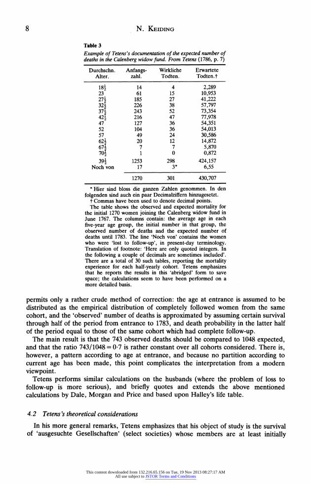
Example of Tetens's documentation of the expected number of deaths in the Calenberg widow fund. From Tetens (1786, p. 7)

Durchschn. Anfangs- Wirkliche Erwartete Alter. zahl. Todten. Todten.t

18' 14 4 2,289 23 61 15 10,953 271 185 27 41,222 32f 226 38 57,797 37f 243 52 73,354 421 216 47 77,978 47 127 36 54,351 52 104 36 54,013 57 49 24 30,586 621 20 12 14,872 67f 7 7 5,870 70' 1 0 0,872 39' 1253 298 424,157

Noch von 17 3* 6,55

1270 301 430,707 * Hier sind bloss die ganzen Zahlen genommen. In den

folgenden sind auch ein paar Decimalziffern hinzugesetzt. t Commas have been used to denote decimal points. The table shows the observed and expected mortality for

the initial 1270 women joining the Calenberg widow fund in June 1767. The columns contain: the average age in each five-year age group, the initial number in that group, the observed number of deaths and the expected number of deaths until 1783. The line 'Noch von' contains the women who were 'lost to follow-up', in present-day terminology. Translation of footnote: 'Here are only quoted integers. In the following a couple of decimals are sometimes included'. There are a total of 30 such tables, reporting the mortality experience for each half-yearly cohort. Tetens emphasizes that he reports the results in this 'abridged' form to save space; the calculations seem to have been performed on a more detailed basis.

permits only a rather crude method of correction: the age at entrance is assumed to be distributed as the empirical distribution of completely followed women from the same cohort, and the 'observed' number of deaths is approximated by assuming certain survival through half of the period from entrance to 1783, and death probability in the latter half of the period equal to those of the same cohort which had complete follow-up.

The main result is that the 743 observed deaths should be compared to 1048 expected, and that the ratio 743/1048 = 0.7 is rather constant over all cohorts considered. There is, however, a pattern according to age at entrance, and because no partition according to current age has been made, this point complicates the interpretation from a modern viewpoint.

Tetens performs similar calculations on the husbands (where the problem of loss to follow-up is more serious), and briefly quotes and extends the above mentioned calculations by Dale, Morgan and Price and based upon Halley's life table.

4. 2 Tetens's theoretical considerations

In his more general remarks, Tetens emphasizes that his object of study is the survival of 'ausgesuchte Gesellschaften' (select societies) whose members are at least initially




healthy, or perhaps initially healthy as well as more permanently strong. Or conversely, unhealthy and possibly also frail.

As an axiom it is assumed that, if the study population mortality is lower than the standard mortality at some age, it stays so with increasing age, but it approaches the latter and ultimately becomes equal to it. In understanding Tetens's desire to have convergent mortalities, due attention should be paid to his above mentioned emphasis on the transient nature of the selectivity. He seems however to be unaware of the consequences of heterogeneity in populations where the frail die first, whereby the population becomes on the average stronger as time goes by (Vaupel, Manton & Stallard, 1979).

The above axiom also has to be seen in the context of Tetens's definition of mortality as the death probability during one time unit (e.g. a year); in fact, this has to equal one at the highest possible age for the study as well as the standard population. Tetens uses an infinitesimal version (what we would call the hazard) in his later mathematical calculations, but does not seem to notice that no requirement of ultimate convergence is needed for mortalities defined as hazards.

Several general properties of the survival curves of the study and standard populations are now derived, such as the impossibility of intersection, and also that, once the difference in survival probability has started to decrease, it will continue to do so.

Of particular interest is what we would call parametric models for the excess (or relative) mortality. These are discussed within the hazard rate framework, and I shall here use modern notation. Let S(x)[So(x)] denote the conditional survival probability given survival to some fixed age xo of entrance into the study [standard] population, so that S(xo) = So(xo) = 1 and S(oo) = So(oo)= 0. Let A(x)[Alo(x)] be the corresponding hazard

rates,A(x) = -D log S(x). The first 'Hypothese', we would say 'model', assumes

= 1 + PSo(x), AO(x)

and is thus a model for relative mortality. As Tetens proves using series expansions (a proof via differential calculus is elementary) it is equivalent to

S(x) = So(x)e(so(x)-1). It is seen that, contrary to our present-day paradigmatic proportional hazards model,

A(x)/Ao(x)-- 1 as x ---> oo; this model for the hazard ratio is perhaps the simplest with this

property. The second model assumes

S(x)= (1 + M)So(x)- -So(x)2,

or equivalently

S(x) - So(x)= M(So(x)- So(x);

thus this model is defined in terms of excess survival probability. The motivation for this model seems to be that it is in some way the simplest satisfying that S(x) = So(x) for x = xo and x = oo and S(x) S(xo) for xo <x < oo

Tetens proves (again using series expansions instead of a modern elementary differential calculus approach) that the model is equivalent to

A(x) 1 + 2aSo(x) - p

Ao(x) 1 + aSo(x) ' 1 +



10 N. KEIDING

and thus again satisfies his requirement of converging hazards, A(x)/AO(x) --1 as x-- oo. As properties of this model Tetens notes first that if > 0 (the case of a healthy study

population) then y < 1. One way of seeing this is to notice that

Y = 1 - A~(xo)/Ao(xo) (4.1)

(this simple representation is not quoted by Tetens). Further, the difference S(x) - So(x) is maximal for So(x) = -, that is at the median survival time ('nach Ablauf des wahrscheinlichen Alters').

Tetens explains in some detail that in order for this model to be useful, experience should show that ~ is constant over age at entrance (our xo) as well as observation period. If this is not the case, however, Tetens recommends the use of an average value of Y

Und diese Zahl wiirde wie ich glaube, gleiche und wohl grossere Zuverlissigkeit haben, als irgend eine unserer besten Mortalitits-Tafeln. (And this number, I think, would have a similar and possibly even higher reliability than any of our best life tables).

For the Calenberg widow fund data, Tetens then goes on to estimate CY for those five-year age groups in each of the separate half-year cohorts which are based on at least 30 (or in some cases 20) initial individuals. The conclusion is that a value of Y = 0.4 could be used for the wives. Further computations are added for the husbands and for the cross-sectional data of Dale, Morgan and Price.

This early attempt at deriving and implementing a simple model for excess mortality deserves mentioning, even though our representation (4.1) shows that

/Y can only be

independent of x0 if A(x)/•A(x)

is constant, which on the other hand violates the converging hazard property, so that no model can accommodate a common ~ for varying age at entrance.

5 Some English contributions in the 19th century

No report touching the history of standardization should bypass the important contributions by 19th century English statisticians. We shall here mention early contributions by F.G.P. Neison and William Farr.

5.1 Neison's sanatory comparison of districts (1844)

In a paper read before the Statistical Society of London in December, 1843, Chadwick (1844) pointed out several shortcomings of (then) current methods of comparing mortality between different classes of the community and between the populations of different districts and countries. As a general rule, Chadwick advocated that the average age at death as well as the average age of the living be quoted and used for these comparative purposes. Four weeks later Neison (1844) read a paper to the Society criticizing Chadwick's in terms that could enter present-day textbooks directly:

That the average age of those who die in one community cannot be taken as a test of the value of life when compared with that in another district is evident from the fact that no two districts or places are under the same distribution of population as to ages ....

Neison calculated for many districts not only the average at death, but

also what would have been the average at death if placed under the same population as the metropolis.

(Direct standardization!)




As example,

This table contains some interesting results, and I beg to cite two cases. The average death in the metropolis is 29-06 years, but in the town of Sheffield it is only 23-19 years; however, if Sheffield were placed under the population of the metropolis the average age at death would be raised to 28-14 years, approaching close to the metropolis.

Neison also remarked that

Another method of viewing this question would be to apply the same rate of mortality to different populations.

(Indirect standardization!)

5.2 Farr's classical explanation of the expected number of deaths

W. Farr (1807-83) worked for many years as 'compiler of abstracts' in the office of the Registrar-General of England. Among his many contributions to mortality statistics is the routine implementation of Neison's suggestion of using expected number of deaths to 'compare local rates of mortality with the standard rate'. For the latter, Farr (1859) chose the average age-specific annual death rates for 1849-53 in the 'healthy districts', which were operationally defined as those with average gross mortality rates of at most foo. Farr's lucid explanation of the method is classical, using,

Example: The number of boys under 5 years of age was 147,390; the annual rate of mortality in the healthy district was 0-04348; and multiplying these two fractions together, 147,390 x 0-04348 = 6367 deaths which would have happened at London had the mortality been at the same rate as it was in the healthy districts.

As conclusion

... on an average, 57,582 persons died in London annually during the five years 1849-53, whereas the deaths should not, at rates of mortality then prevailing in certain districts of England, have exceeded 36,179; consequently 21,403 unnatural deaths took place every year in London. It will be the office of the Boards of Works to reduce this dreadful sacrifice of life to the lowest point, and thus to deserve well of their country.

5.3 Was the method of expected number of deaths reinvented in 19th century England? I have found no reference to the use of the method of expected number of deaths in the

18th century actuarial context from the later English authors, who were concerned primarily with geographical or occupational variations of mortality. In fact, I have not met Dale's name outside of the above mentioned references by Price and Tetens, and as regards Tetens's contribution to the method of expected number of deaths, I have seen no other reference than that by Westergaard (1932), who gave a brief reference to the practical calculation, but did not mention the parametric statistical models. It would be of considerable interest in this context to explore Neison's background further.

Tetens also contributed other innovations in actuarial mathematics, and one of these, the 'commutation method' was independently (so it has to be assumed) invented by George Barnett in England and published by Francis Baily. Hendriks (1851) reintroduced this contribution of Tetens to the English actuarial community, and in this connection enquired about any evidence in Price's papers about Price having known about Tetens's work. Such evidence would certainly be rather interesting in our context, too. (Price died in 1791, five years after the publication of Tetens's second volume).



12 N. KEIDING

6 Westergaard

Harald Westergaard (1853-1936) had degrees from the University of Copenhagen in both economics and mathematics. Before becoming professor in economics and statistics at this university, Westergaard had studied in England and other European countries and he presented his considerable knowledge of mortality and morbidity in a prize paper to the university in 1880. This was quickly published in German, Die Lehre von der Mortalitiit und Morbilitiit (Westergaard, 1882), and reissued in a completely revised version in 1901. From the point of view of the method of expected number of deaths the first edition is however the more interesting.

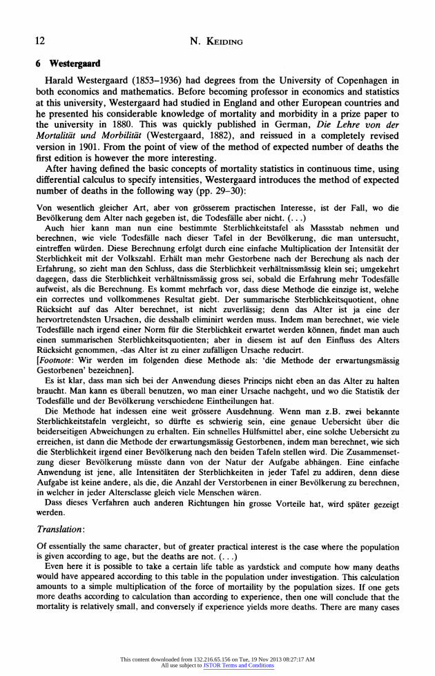
After having defined the basic concepts of mortality statistics in continuous time, using differential calculus to specify intensities, Westergaard introduces the method of expected number of deaths in the following way (pp. 29-30): Von wesentlich gleicher Art, aber von gr6sserem practischen Interesse, ist der Fall, wo die Bev61lkerung dem Alter nach gegeben ist, die Todesfiille aber nicht. (...)

Auch hier kann man nun eine bestimmte Sterblichkeitstafel als Massstab nehmen und berechnen, wie viele Todesfiille nach dieser Tafel in der Bev61lkerung, die man untersucht, eintreffen wiirden. Diese Berechnung erfolgt durch eine einfache Multiplication der Intensitit der Sterblichkeit mit der Volkszahl. Erhilt man mehr Gestorbene nach der Berechung als nach der Erfahrung, so zieht man den Schluss, dass die Sterblichkeit verhiltnissmissig klein sei; umgekehrt dagegen, dass die Sterblichkeit verhiltnissmissig gross sei, sobald die Erfahrung mehr Todesfille aufweist, als die Berechnung. Es kommt mehrfach vor, dass diese Methode die einzige ist, welche ein correctes und vollkommenes Resultat giebt. Der summarische Sterblichkeitsquotient, ohne Riicksicht auf das Alter berechnet, ist nicht zuverlissig; denn das Alter ist ja eine der hervortretendsten Ursachen, die desshalb eliminirt werden muss. Indem man berechnet, wie viele Todesfille nach irgend einer Norm fiir die Sterblichkeit erwartet werden k6nnen, findet man auch einen summarischen Sterblichkeitsquotienten; aber in diesem ist auf den Einfluss des Alters Riicksicht genommen, -das Alter ist zu einer zufilligen Ursache reducirt. [Footnote: Wir werden im folgenden diese Methode als: 'die Methode der erwartungsmissig Gestorbenen' bezeichnen].

Es ist klar, dass man sich bei der Anwendung dieses Princips nicht eben an das Alter zu halten braucht. Man kann es iiberall benutzen, wo man einer Ursache nachgeht, und wo die Statistik der Todesfaille und der Bev61lkerung verschiedene Eintheilungen hat.

Die Methode hat indessen eine weit gr6ssere Ausdehnung. Wenn man z.B. zwei bekannte Sterblichkeitstafeln vergleicht, so diirfte es schwierig sein, eine genaue Uebersicht iiber die beiderseitigen Abweichungen zu erhalten. Ein schnelles Hiilfsmittel aber, eine solche Uebersicht zu erreichen, ist dann die Methode der erwartungsmissig Gestorbenen, indem man berechnet, wie sich die Sterblichkeit irgend einer Bev61lkerung nach den beiden Tafeln stellen wird. Die Zusammenset- zung dieser Bevilkerung miisste dann von der Natur der Aufgabe abhingen. Eine einfache Anwendung ist jene, alle Intensititen der Sterblichkeiten in jeder Tafel zu addiren, denn diese Aufgabe ist keine andere, als die, die Anzahl der Verstorbenen in einer Bev61lkerung zu berechnen, in welcher in jeder Altersclasse gleich viele Menschen wiren.

Dass dieses Verfahren auch anderen Richtungen hin grosse Vorteile hat, wird spiter gezeigt werden.

Translation:

Of essentially the same character, but of greater practical interest is the case where the population is given according to age, but the deaths are not. (...)

Even here it is possible to take a certain life table as yardstick and compute how many deaths would have appeared according to this table in the population under investigation. This calculation amounts to a simple multiplication of the force of mortaility by the population sizes. If one gets more deaths according to calculation than according to experience, then one will conclude that the mortality is relatively small, and conversely if experience yields more deaths. There are many cases




where this method is the only way to obtain a correct and complete result. The summary mortality ratio calculated without regard to age is unreliable; for age is one of the more important causes which therefore has to be eliminated. By calculating how many deaths may be expected according to some mortality standard one also obtains a summary mortality ratio; however, in this the influence of age has been taken into consideration-age has been reduced to a random cause. [Footnote: We shall in the following denote this method 'the method of expected deaths'].

It is obvious that it is not necessary to restrict oneself to age when applying this principle, anytime one searches for a cause, and mortality and population statistics have different classifications, it can be applied.

The method has however a much wider application. If one for instance compares two known life tables it may be difficult to obtain a clear impression about the deviations. A quick tool to provide such an impression is then the method of expected deaths, where one calculates how the mortality of some population would be according to the two tables. The composition of this population should depend on the nature of the problem. A simple application of this is to add all forces of mortality in each table, since this just amounts to calculating the number of deaths in a population with an equal number of persons in each age class.

That this method also has great advantages in other directions will be shown later.

We note in passing that the idea of just adding all forces of mortality was reintroduced

by Yule (1934) and later by Day (1976), who applied it to world-wide cancer incidence

comparisons.

6.1 Confounder control and precision

In his introduction of the method of expected deaths, Westergaard emphasizes what would today be termed confounder control: 'das Alter ist zu einer zufailligen Ursache reducirt', age is 'reduced to a random cause' when the incidence or mortality between two

populations is to be compared. If there are more than one 'stoirende Ursache' (we would

say: confounder), Westergaard recommends further subdivisions, since as he sees the method of expected number of events, it can only eliminate one confounder.

Although confounder control is discussed more thoroughly here than in most earlier literature, Westergaard's approach to sampling variablity and its interaction with the method of expected number of events seems to be his particularly innovative contribution. The concept of distribution of observed events is introduced, and the 'mittlere Fehler' (standard error) is defined as the distance between mode and point of inflection of the normal density (here called 'die Exponentialformel'). The observed number of deaths d has mean error V/(Spq), where S is population size and p = 1 - q the death probability. Westergaard notes that often p is rather small, so that q is almost 1, and the useful

approximation V(Sp) = Vd is obtained: we would call this a Poisson approximation. Westergaard goes on to explain that one should in practice always investigate the

applicability of this standard error (through derived fractiles of the distribution) and, if the variability is greater than the 'theoretical', there will be heterogeneities which should be removed by further subdivision.

6.2 Rubin & Westergaard's study of occupational mortality, 1886

At the request of the director of the Danish National Bank, who wanted a better statistical basis for current political discussions on social issues, Westergaard (with Marcus Rubin) carried out an investigation of the mortality, as specified by occupational classes, of the rural population of the diocese of Fyen, about 170,000 persons (Rubin &



14 N. KEIDING

Westergaard, 1886). Unfortunately this report is available in Danish only, save for a brief German summary without methodological remarks (Westergaard, 1887).

Unusual care has been taken in this investigation to match 'numerator' and 'denominator' populations. The deaths were based upon medical and church records for the period 1876-83 around the census 1880, from which the classification of the living was taken. Further, the occupational classifications of both living and dead were scrutinized and reported by local assistants, primarily schoolteachers.

Of particular interest in our context is the consistent analytical-statistical viewpoint in the methodological introduction and throughout the discussion of the results. Thus (pp. 56-57, my translation):

Since, however, the data are usually too few, it is necessary to quote the mortality ratios with some reservation, as far as possible combined with limits for the errors by which the ratios are vitiated. In the present investigation this has been done using the standard error....

The method by which it is possible in this way to eliminate the influence of age, the 'method of expected deaths' thus consists in calculating the mortality which would have appeared if the conditions within each age group were in close accordance with the mortality conditions according to some known life table, for instance that for the whole population or the agrarian class. If then the total number of deaths, relative to the standard error, shows a considerable deviation from what would be normal for the relevant group, when the mortality corresponded to the used life table, then there is reason to believe that there exist causes which particularly influence the health status in the particular occupations, even if this due to the limited size of the data cannot be concluded with certainty for the single age classes of the occupation.

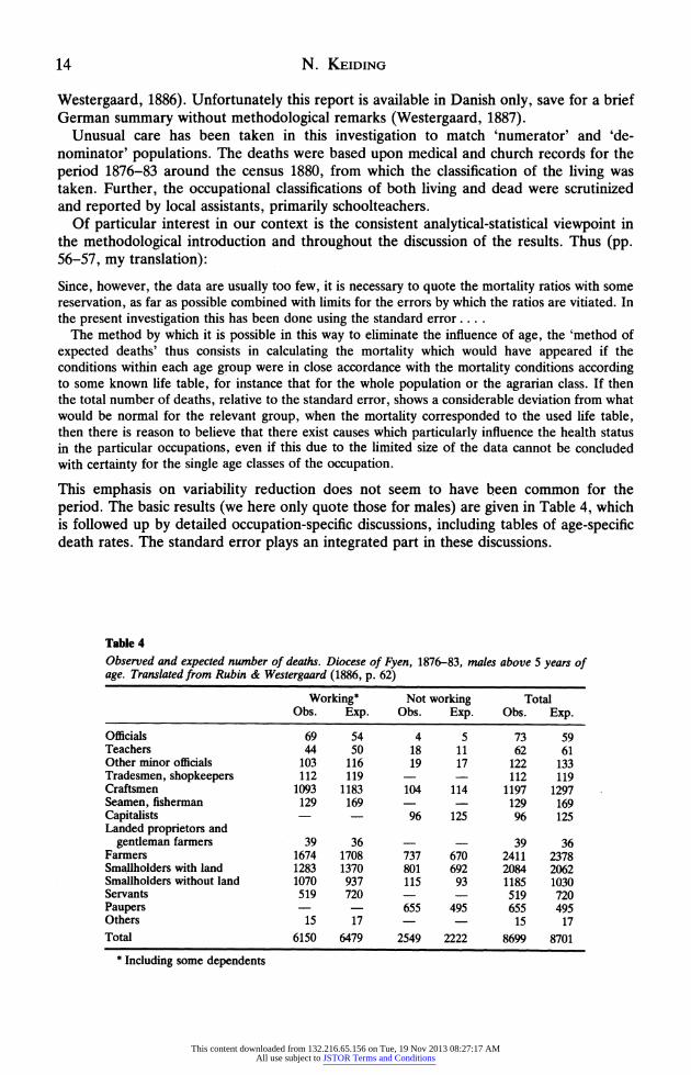
This emphasis on variability reduction does not seem to have been common for the period. The basic results (we here only quote those for males) are given in Table 4, which is followed up by detailed occupation-specific discussions, including tables of age-specific death rates. The standard error plays an integrated part in these discussions.

Table 4 Observed and expected number of deaths. Diocese of Fyen, 1876-83, males above 5 years of age. Translated from Rubin & Westergaard (1886, p. 62)

Working* Not working Total Obs. Exp. Obs. Exp. Obs. Exp.

Officials 69 54 4 5 73 59 Teachers 44 50 18 11 62 61 Other minor officials 103 116 19 17 122 133 Tradesmen, shopkeepers 112 119 - - 112 119 Craftsmen 1093 1183 104 114 1197 1297 Seamen, fisherman 129 169 - - 129 169 Capitalists - - 96 125 96 125 Landed proprietors and

gentleman farmers 39 36 - - 39 36 Farmers 1674 1708 737 670 2411 2378 Smallholders with land 1283 1370 801 692 2084 2062 Smallholders without land 1070 937 115 93 1185 1030 Servants 519 720 - - 519 720 Paupers - - 655 495 655 495 Others 15 17 - - 15 17 Total 6150 6479 2549 2222 8699 8701

* Including some dependents




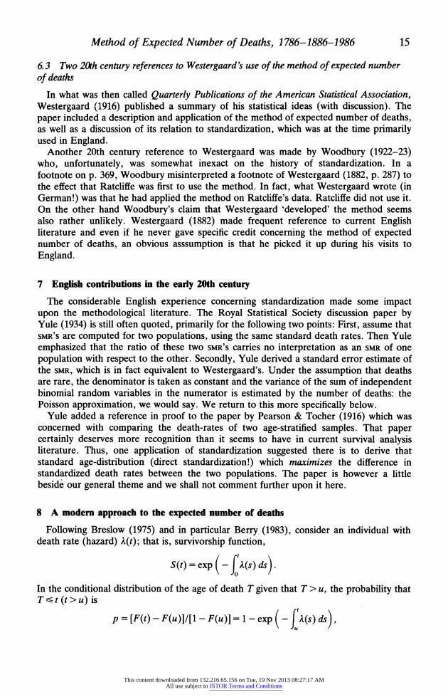
6.3 Two 20th century references to Westergaard's use of the method of expected number of deaths

In what was then called Quarterly Publications of the American Statistical Association, Westergaard (1916) published a summary of his statistical ideas (with discussion). The paper included a description and application of the method of expected number of deaths, as well as a discussion of its relation to standardization, which was at the time primarily used in England.

Another 20th century reference to Westergaard was made by Woodbury (1922-23) who, unfortunately, was somewhat inexact on the history of standardization. In a footnote on p. 369, Woodbury misinterpreted a footnote of Westergaard (1882, p. 287) to the effect that Ratcliffe was first to use the method. In fact, what Westergaard wrote (in German!) was that he had applied the method on Ratcliffe's data. Ratcliffe did not use it. On the other hand Woodbury's claim that Westergaard 'developed' the method seems also rather unlikely. Westergaard (1882) made frequent reference to current English literature and even if he never gave specific credit concerning the method of expected number of deaths, an obvious asssumption is that he picked it up during his visits to England.

7 English contributions in the early 20th century

The considerable English experience concerning standardization made some impact upon the methodological literature. The Royal Statistical Society discussion paper by Yule (1934) is still often quoted, primarily for the following two points: First, assume that SMR'S are computed for two populations, using the same standard death rates. Then Yule emphasized that the ratio of these two SMR'S carries no interpretation as an SMR of one population with respect to the other. Secondly, Yule derived a standard error estimate of the SMR, which is in fact equivalent to Westergaard's. Under the assumption that deaths are rare, the denominator is taken as constant and the variance of the sum of independent binomial random variables in the numerator is estimated by the number of deaths: the Poisson approximation, we would say. We return to this more specifically below.

Yule added a reference in proof to the paper by Pearson & Tocher (1916) which was concerned with comparing the death-rates of two age-stratified samples. That paper certainly deserves more recognition than it seems to have in current survival analysis literature. Thus, one application of standardization suggested there is to derive that standard age-distribution (direct standardization!) which maximizes the difference in standardized death rates between the two populations. The paper is however a little beside our general theme and we shall not comment further upon it here.

8 A modem approach to the expected number of deaths

Following Breslow (1975) and in particular Berry (1983), consider an individual with death rate (hazard) A(t); that is, survivorship function,

S(t) = exp( - A( ds).

In the conditional distribution of the age of death T given that T > u, the probability that T ~ t (t>u) is

p = [F(t) - F(u)l/[1 - F(u)l = 1 - exp - A(s) ds ,



16 N. KEIDING

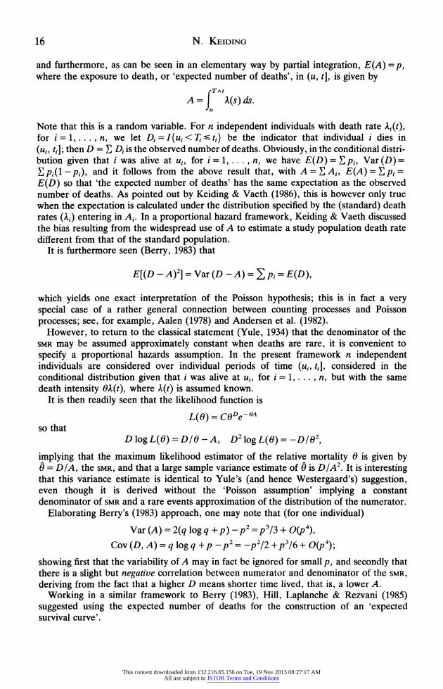
and furthermore, as can be seen in an elementary way by partial integration, E(A) =p, where the exposure to death, or 'expected number of deaths', in (u, t], is given by

A = fAt(s) ds.

Note that this is a random variable. For n independent individuals with death rate Ai(t), for i = 1,... , n, we let Di = I{u, < T- < ti} be the indicator that individual i dies in

(ui, ti]; then D = , D, is the observed number of deaths. Obviously, in the conditional distribution given that i was alive at ui, for i = 1,... , n, we have E(D) = pi, Var (D) =

E pi(l -pP), and it follows from the above result that, with A = Ai, E(A) = F pi =

E(D) so that 'the expected number of deaths' has the same expectation as the observed number of deaths. As pointed out by Keiding & Vaeth (1986), this is however only true when the expectation is calculated under the distribution specified by the (standard) death rates (A•) entering in A,. In a proportional hazard framework, Keiding & Vaeth discussed the bias resulting from the widespread use of A to estimate a study population death rate different from that of the standard population.

It is furthermore seen (Berry, 1983) that

E[(D - A)2] = Var (D - A) = > pi = E(D),

which yields one exact interpretation of the Poisson hypothesis; this is in fact a very special case of a rather general connection between counting processes and Poisson processes; see, for example, Aalen (1978) and Andersen et al. (1982).

However, to return to the classical statement (Yule, 1934) that the denominator of the SMR may be assumed approximately constant when deaths are rare, it is convenient to specify a proportional hazards assumption. In the present framework n independent individuals are considered over individual periods of time (ui, ti], considered in the conditional distribution given that i was alive at ui, for i = 1,... , n, but with the same death intensity OA(t), where A(t) is assumed known.

It is then readily seen that the likelihood function is

L(O) = CODe-OA

so that D log L(O) = DIO - A, D2 log L(O) = -D/2,

implying that the maximum likelihood estimator of the relative mortality 0 is given by 0 = DIA, the SMR, and that a large sample variance estimate of 0 is D/A2. It is interesting that this variance estimate is identical to Yule's (and hence Westergaard's) suggestion, even though it is derived without the 'Poisson assumption' implying a constant denominator of SMR and a rare events approximation of the distribution of the numerator.

Elaborating Berry's (1983) approach, one may note that (for one individual)

Var (A) = 2(q log q + p) -p2 = p3/3 + O(p4),

Cov (D, A) = q log q +p -p2 = -p2/2 +p3/6 + O(p4);

showing first that the variability of A may in fact be ignored for small p, and secondly that there is a slight but negative correlation between numerator and denominator of the SMR, deriving from the fact that a higher D means shorter time lived, that is, a lower A.

Working in a similar framework to Berry (1983), Hill, Laplanche & Rezvani (1985) suggested using the expected number of deaths for the construction of an 'expected survival curve'.




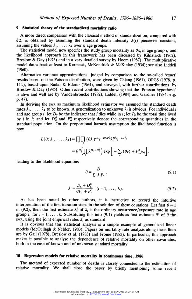
9 Statistical theory of the standardized mortality ratio

A more direct comparison with the classical method of standardization, compared with ? 2, is obtained by assuming the standard death intensity A(t) piecewise constant, assuming the values

A1, .. , , .k over k age groups.

The statistical model now specifies the study group mortality as •xi in age group i, and the likelihood approach in this framework has been discussed by Kilpatrick (1962), Breslow & Day (1975) and in a very detailed survey by Hoem (1987). The multiplicative model dates back at least to Kermack, McKendrick & McKinlay (1934); see also Liddell (1960).

Alternative variance approximations, judged by comparison to the so-called 'exact' results based on the Poisson distribution, were given by Chiang (1961), OPCS (1978, p. 14f.), based upon Bailar & Ederer (1964), and surveyed, with further contributions, by Breslow & Day (1985). Other recent contributions showing that the 'Poisson hypothesis' is alive and well are by Vandenbroucke (1982), Liddell (1984) and Gardner (1984, e.g. p. 47).

In deriving the SMR as maximum likelihood estimator we assumed the standard death rates A•,

.?. ? , Ik to be known. A generalization to unknown k, is obvious. For individual j

and age group i, let Dij be the indicator that j dies while in i; let P,, be the total time lived by j in i; and let DO and PO respectively denote the corresponding quantities in the standard population. On the proportional hazards assumption the likelihood function is now

L(O; •,.. ., k)' = HH (OAi) ije -?19'PiP(1)iA QJe-`iP

If

i j

= GD (171ADi+) exp [- (OBP + P9+

leading to the likelihood equations D

0= , (9.1)

D. + D9 Ai=(i =

1,..., k). (9.2) oP; + P9

As has been noted by other authors, it is instructive to record the intuitive interpretation of the first iteration steps in the solution of these equations. Let first 0 = 1 in (9.2), then the first estimate A! of Ai, is the ordinary occurrence/exposure rate in age group i, for i = 1,... , k. Substituting this into (9.1) yields as first estimate 01 of 0 the SMR, using the joint empirical rates kA) as standard.

It is obvious that this statistical analysis is a simple example of generalized linear models (McCullagh & Nelder, 1983). Papers on mortality rate analysis along these lines are by Gail (1978), Breslow et al. (1983) and Frome (1983). In particular, this approach makes it possible to analyse the dependence of relative mortality on other covariates, both in the case of known and of unknown standard mortality.

10 Regression models for relative mortality in continuous time, 1986

The method of expected number of deaths is closely connected to the estimation of relative mortality. We shall close the paper by briefly mentioning some recent



18 N. KEIDING

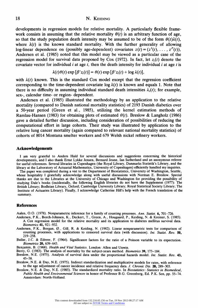
developments in regression models for relative mortality. A particularly flexible framework consists in assuming that the relative mortality 0(t) is an arbitrary function of age, so that the study population death intensity may be assumed to be of the form 0(t)Z(t), where A(t) is the known standard mortality. With the further generality of allowing log-linear dependence on (possibly age-dependent) covariates z(t) = (z'(t),..., zP(t)), Andersen et al. (1985) noted that this model may be viewed as a particular case of the regression model for survival data proposed by Cox (1972). In fact, let z,(t) denote the covariate vector for individual i at age t, then the death intensity for individual i at age t is

A(t)O (t) exp [P'zi(t)] = 6(t) exp [P'zi(t) + log A(t)],

with A(t) known. This is the standard Cox model except that the regression coefficient corresponding to the time-dependent covariate log

A,(t) is known and equals 1. Note that

there is no difficulty in assuming individual standard death intensities A•,(t); for example, sex-, calendar time- or region- dependent.

Andersen et al. (1985) illustrated the methodology by an application to the relative mortality (compared to Danish national mortality statistics) of 2193 Danish diabetics over a 50-year period (Green et al., 1985), utilizing the kernel estimation methods of Ramlau-Hansen (1983) for obtaining plots of estimated 0(t). Breslow & Langholz (1986) gave a detailed further discussion, including consideration of possibilities of reducing the computational effort in large cohorts. Their study was illustrated by application to the relative lung cancer mortality (again compared to relevant national mortality statistics) of cohorts of 8014 Montana smelter workers and 679 Welsh nickel refinery workers.

Acknowledgements I am very grateful to Anders Hald for several discussions and suggestions concerning the historical

developments, and I also thank Ernst Lykke Jensen, Bernard Jeune, Ian Sutherland and an anonymous referee for useful references. Several libraries in Copenhagen (the Royal Library, Danmarks Statistik's Library, and the library at the Laboratory of Actuarial Mathematics, University of Copenhagen) efficiently handled my inquiries.

The paper was completed during a vist to the Department of Biostatistics, University of Washington, Seattle, whose hospitality I gratefully acknowledge along with useful discussions with Norman E. Breslow. Special thanks are due to the Libraries at the University of Chicago and Washington for providing the possibility of studying Dale's books (incidentally, the following English libraries do not have the Supplement (1977): The British Library; Bodleian Library, Oxford; Cambridge University Library; Royal Statistical Society Library; The Institute of Actuaries Library). Finally, I acknowledge Catherine Hill's help with the French translation of the summary.

References

Aalen, 0.0. (1978). Nonparametric inference for a family of counting processes. Ann. Statist. 6, 701-726. Andersen, P.K., Borch-Johnsen, K., Deckert, T., Green, A., Hougaard, P., Keiding, N. & Kreiner, S. (1985).

A Cox regression model for the relative mortality and its application to diabetes mellitus survival data. Biometrics 41, 921-932.

Andersen, P.K., Borgan, 0., Gill, R. & Keiding, N. (1982). Linear nonparametric tests for comparison of counting processes, with applications to censored survival data (with discussion). Int. Statist. Rev. 50, 219-258.

Bailar, J.C. & Ederer, F. (1964). Significance factors for the ratio of a Poisson variable to its expectation. Biometrics 20, 639-643.

Benjamin, B. (1968). Health and Vital Statistics. London: Allen and Unwin. Berry, G. (1983). The analysis of mortality by the subject-years method. Biometrics 39, 173-184. Breslow, N.E. (1975). Analysis of survival data under the proportional hazards model. Int. Statist. Rev. 43,

45-58. Breslow, N.E. & Day, N.E. (1975). Indirect standardization and multiplicative models for rates, with reference

to the age adjustment of cancer incidence and relative frequency data. J. Chronic Dis. 28, 289-303. Breslow, N.E. & Day, N.E. (1985). The standardized mortality ratio. In Biostatistics: Statistics in Biomedical,

Public Health and Environmental Sciences in honor of Professor B.G. Greenberg, Ed. P.K. Sen, pp. 55-74. Amsterdam: North-Holland.




Breslow, N.E. & Langholz, B. (1986). Nonparametric estimation of relative mortality functions. J. Chronic Dis. To appear.

Breslow, N.E., Lubin, J.H., Marek, P. & Langholz, B. (1983). Multiplicative models and cohort analysis. J. Am. Statist. Assoc. 78, 1-12.

Chadwick, E. (1844). On the best modes of representing accurately, by statistical returns, the duration of life, and the pressure and progress of the causes of mortality amongst different classes of the community, and amongst the populations of different districts and countries. J. Statist. Soc. (London) 7, 1-40.

Chiang, C.L. (1961). Standard error of the age-adjusted death ratio. Vital Statistics, Special Reports Selected Studies 47, 275-285. National Center for Health Statistics.

Cox, D.R. (1972). Regression models and life-tables (with discussion). J.R. Statist. Soc. B 34, 187-220. [Dale, W.] (1772). Calculations Deduced from First Principles, in the Most Familiar Manner, by Plain

Arithmetic, for the Use of the Societies Instituted for the Benefit of Old Age: Intended as an Introduction to the Study of the Doctrine of Annuities. By a Member of One of the Societies. London: J. Ridley.

[Dale, W.] (1777). A Supplement to Calculations of the Value of Annuities, Published for the Use of Societies Instituted for Benefit of Age Containing Various Illustration of the Doctrine of Annuities, and Compleat Tables of the Value of 1?. Immediate Annuity. (Being the Only Ones Extant by Half-Yearly Interest and Payments). Together with Investigations of the State of the Laudable Society of Annuitants; Showing What Annuity Each Member Hath Purchased, and Real Mortality Therein, from its Institution Compared with Dr. Halley's Table. Also Several Publications, Letters, and Anecdotes Relative to that Society. And Explanatory of Proceedings to the Present Year. London: Ridley.

Day, N.E. (1976). A new measure of age standardized incidence, the cumulative rate. In Cancer Incidence in Five Continents, 3, Ed. J. Waterhouse, C. Muir, P. Correa and J. Powell, pp. 443-445. Lyon: International agency for Research on Cancer.

Farr, W. (1859). Letter to the Registrar General. Appendix to the 20th Annual Report of the Registrar General for England and Wales. London: General Registrar Office.

Frome, E.L. (1983). The analysis of rates using Poisson regression models. Biometrics 39, 665-674. Gail, M. (1978). The analysis of heterogeneity for indirect standardized mortality ratios. J.R. Statist. Soc. A 141,

224-234. Gardner, M. (Ed.) (1984). Expected Numbers in Cohort Studies. Southampton: MRC Environmental

Epidemiology Unit. Green, A., Borch-Johnsen, K., Andersen, P.K., Hougaard, P., Keiding, N., Kreiner, S. & Deckert, T. (1985).

Relative mortality of type I (insulin-dependent) diabetes in Denmark (1933-1981). Diabetologia 28, 339-342.

Hendriks, F. (1851). Memoir of the early history of auxiliary tables for the computation of life contingencies. Ass. Mag. (J. Inst. Act.) 1 (1), 1-20.

Hill, C., Laplanche, A. & Rezvani, A. (1985). Comparison of the mortality of a cohort with the mortality of a reference population in a prognostic study. Statist. Medicine 4, 295-302.

Hoem, J.M. (1987). Statistical analysis of a multiplicative model and its application to the standardization of vital rates: A review. Int. Statist. Rev. 55. To appear.

Inskip, H., Beral, V. & Fraser, P. (1983). Methods for age-adjustment of rates. Statist. Medicine 2, 455-466. Keiding, N. & Vaeth, M. (1986). Calculating expected mortality. Statist. Medicine 5, 327-334. Kermack, W.O., McKendrick, A.G. & McKinlay, P.L. (1934). Death-rates in Great Britain and Sweden:

Expression of specific mortality rates as products of two factors, and some consequences thereof. J. Hygiene 34, 433-457.

Kilpatrick, S.J. (1962). Occupational mortality indices. Population Studies 16, 175-187. Liddell, F.D.K. (1960). The measurement of occupational mortality. Br. J. Indust. Med. 17, 228-223. Liddell, F.D.K. (1984). Simple exact analysis of the standardized mortality ratio. J. Epidemiol. Community

Health 38, 85-88. Lilienfeld, D.E. (1978). "The greening of epidemiology": Sanitary physicians and the London epidemiological

society (1830-1870). Bull. Hist. Medicine 52, 503-528. Logan, W.P.D. (1982). Cancer Mortality by Occupation and Social Class 1851-1971. London: Her Majesty's

Stationery Office; Lyon: International Agency for Research on Cancer. McCullagh, P. & Nelder, J. (1983). Generalized Linear Models. London: Chapman and Hall. Monson, R.R. (1974). Analysis of relative survival and proportional mortality. Comp. Biomed. Res. 7, 325-332. Morgan, W. (1779). The Doctrine of Annuities and Assurances on Lives and Survivorships, Stated and

Explained. London: Cadell. Neison, F.G.P. (1844). On a method recently proposed for conducting inquiries into the comparative sanatory

condition of various districts, with illustrations, derived from numerous places in Great Britain at the period of the last census. J. Statist. Soc. (London) 7, 40-68.

Office of Population Censuses and Surveys. (1978). Occupational Mortality 1970-72; Decennial Supplement. Series DS No. 1. London: Her Majesty's Stationery Office.

Pearson, K. & Tocher, J.F. (1916). On criteria for the existence of differential deathrates. Biometrika 11, 157-184.

Price, R. (1771, 1783). Observations on Reversionary Payments; On Schemes for Providing Annuities for Widows, and for Persons in Old Age; on the Method of Calculating the Values of Assurances on Lives, and on the National Debt. First and 4th ed. London: Cadell.



20 N. KEIDING

Price, R. (1983). The Correspondence of Richard Price I: July 1748-March 1778, Ed. W.B. Peach and D.O. Thomas. Durham, N.C.: Duke University Press.

Ramlau-Hansen, H. (1983). Smoothing counting process intensities by means of kernel functions. Ann. Statist. 11, 453-466.

Rubin, M. & Westergaard, H. (1886). Landbefolkningens dodelighed i Fyens Stift (Mortality of the Rural Population in the Diocese of Funen). Copenhagen: P.G. Philipsen.

Tetens, J.N. (1786). Einleitung zur Berechnung der Leibrenten und Anwartschaften II. Leipzig: Weidmanns Erben und Reich.

Tetens, J.N. (1971). Sprachphilosophische Versuche. Mit einer Einleitung von E. Heintel, herausgegeben von H. Pfannkuch. Hamburg: Meiner.

Vandenbroucke, J.P. (1982). A shortcut method for calculating the 95 per cent confidence interval of the standardized mortality ratio. Am. J. Epidemiol. 115, 303-304.

Vaupel, J.W., Manton, K.G. & Stallard, E. (1979). The impact of heterogeneity in individual frailty on the dynamics of mortality. Demography 16, 439-454.

Westergaard, H. (1882). Die Lehre von der Mortalitiit und Morbilitiit. Jena: Fischer. Westergaard, H. (1887). Die Sterblichkeit in den verschiedenen Gesellschaftsclassen der Landbev61lkerung

Diinemarks. Assecuranz-Jahrbuch 8, 72-79. Westergaard, H. (1916). Scope and methods of statistics (with discussion). Quart. Publ. Am. Statist. Assoc. 15,

225-291. Westergaard, H. (1932). Contributions to the History of Statistics. London: King. Woodbury, R.M. (1922-23). Westergaard's method of expected deaths as applied to the study of infant

mortality. J. Am. Statist. Assoc. 18, 366-376. Yule, G.U. (1934). On some points relating to vital statistics, more especially statistics of occupational mortality

(with discussion). J.R. Statist. Soc. 97, 1-84.

R6sume La m6thode du nombre de d6ces attendus est partie int6grante de la standardisation des taux vitaux, qui est

l'une des plus anciennes techniques statistiques. Le nombre de d6chs attendus 6tait calcul6 au XVIIIe sidcle en math6matiques d'assurance (Dale, 1777; Tetens, 1786). Donc, la m6thode semble oubli6e pour 8tre retrouv6e au XIXe si•cle en 6tudes des variations gdographiques et professionelles de la mortalit6 (Neison, 1844: Farr, 1859; Westergaard, 1882; Rubin & Westergaard, 1886). On note que la standardisation des taux est 6troitement li6e l'6tude de la mortalit6 relative. Les d6veloppements r6cents de la m6thodologie dans ce domaine sont bribvement decrits.

[Received December 1985, revised February 1986]



The Method of Expected Number of Deaths, 1786-1886-1986 ... · Method of Expected Number of Deaths,...

Documents

Transcript of The Method of Expected Number of Deaths, 1786-1886-1986 ... · Method of Expected Number of Deaths,...