The MERLIN-Expo Soil model V1 · 2015-10-30 · The Soil model assumes that contaminants are...
107
1 The MERLIN-Expo Soil model V1.3 Author : Philippe Ciffroy EDF R&D, 6 quai Watier, 78400 Chatou, France [email protected] Reviewers : James Garratt 1 , Erik Johansson 2 , Boris Alfonso 2 1 Enviresearch Ltd, Nanotechnology Centre, Newcastle University, Newcastle upon Tyne NE1 7RU, UK 2 FACILIA, Gustavslundsvägen 151C 167 51 Bromma, Sweden
Transcript of The MERLIN-Expo Soil model V1 · 2015-10-30 · The Soil model assumes that contaminants are...

1
The MERLIN-Expo Soil model
V1.3
Author: Philippe Ciffroy
EDF R&D, 6 quai Watier, 78400 Chatou, France
Reviewers: James Garratt1, Erik Johansson2, Boris Alfonso2 1Enviresearch Ltd, Nanotechnology Centre, Newcastle University, Newcastle upon Tyne NE1
7RU, UK 2 FACILIA, Gustavslundsvägen 151C 167 51 Bromma, Sweden

2
Sommaire
LEVEL 1 DOCUMENTATION (BASIC KNOWLEDGE ON MODEL PURPOSE, APPLICABILITY AND COMPONENTS) .. 5
1. MODEL PURPOSE ..................................................................................................................................... 5
1.1. GOAL ....................................................................................................................................................... 5
1.2. POTENTIAL DECISION AND REGULATORY FRAMEWORK(S) .................................................................................... 5
2. MODEL APPLICABILITY ............................................................................................................................. 6
2.1. SPATIAL SCALE AND RESOLUTION .................................................................................................................... 6
2.2. TEMPORAL SCALE AND RESOLUTION................................................................................................................ 6
2.3. CHEMICAL CONSIDERED ............................................................................................................................... 6
2.4. STEADY-STATE VS DYNAMIC PROCESSES ........................................................................................................... 7
3. MODEL COMPONENTS ............................................................................................................................. 7
3.1. MEDIA CONSIDERED .................................................................................................................................... 7
3.2. LOADINGS ................................................................................................................................................. 8
3.3. LOSSES ................................................................................................................................................... 10
3.4. EXCHANGES BETWEEN MODEL MEDIA ........................................................................................................... 12
3.5. POTENTIAL COUPLED MODELS ..................................................................................................................... 13
3.6. FORCING VARIABLES .................................................................................................................................. 16
3.7. PARAMETERS ........................................................................................................................................... 21
3.8. INTERMEDIATE STATE VARIABLES ................................................................................................................. 25
3.9. REGULATORY STATE VARIABLES ................................................................................................................... 33
LEVEL 2 DOCUMENTATION (BACKGROUND SCIENCE) ..................................................................................... 37
4. PROCESSES AND ASSUMPTIONS ............................................................................................................ 37
4.1. PROCESS N°1: SORPTION/DESORPTION BETWEEN PORE WATER AND SOIL PARTICLES ............................................. 37
4.2. PROCESS N°2: EVAPOTRANSPIRATION ........................................................................................................... 37
4.3. PROCESS N°3: WATER MASS BALANCE IN SOIL AND LOSS BY INFILTRATION............................................................ 38
4.4. PROCESS N°4: RETARDATION FACTOR AND ADVECTION WITHIN SOIL ................................................................... 39
4.5. PROCESS N°5: DIFFUSION BETWEEN SOIL AND ATMOSPHERE (ONLY FOR ORGANICS) .............................................. 41
4.6. PROCESS N°6: BIOTURBATION ..................................................................................................................... 42
4.7. PROCESS N°7: DIFFUSION WITHIN SOIL ......................................................................................................... 43
4.8. PROCESS N°8: WASH-OFF FROM SOILS TO RIVER ............................................................................................. 45
4.9. PROCESS N°9: DEGRADATION (ONLY FOR ORGANICS) ...................................................................................... 46
LEVEL 3 DOCUMENTATION (NUMERICAL INFORMATION) .............................................................................. 47
5. NUMERICAL DEFAULT VALUES (DETERMINISTIC AND/OR PROBABILISTIC) ............................................ 47
5.1. INITIALIZATION OF CONCENTRATIONS IN MEDIA .............................................................................................. 47
5.2. DEFAULT PARAMETER VALUES ..................................................................................................................... 47
5.3.1 Site-specific parameters ...................................................................................................................... 47 5.3.1.1 Soil surface ..................................................................................................................................................... 47 5.3.1.2 Depth of the root zone .................................................................................................................................. 48 5.3.1.3 Number of soil layers ..................................................................................................................................... 49
5.3.2 Soil physico-chemical properties of soil ............................................................................................... 50

3
5.3.2.1 Dry density of soil .......................................................................................................................................... 50 5.3.2.2 Soil water content at field capacity ................................................................................................................ 51 5.3.2.3 Soil water content at wilting point ................................................................................................................. 51 5.3.2.4 Moisture stress .............................................................................................................................................. 54
5.3.3 Parameters related to partition between phases ................................................................................ 55 5.3.3.1 Water-organic carbon partition coefficient (for Organics only) ..................................................................... 55 5.3.3.2 Fraction of organic matter in soil (for Organics only) .................................................................................... 62 5.3.3.4 Water-Soil partition coefficient (for Metals only) .......................................................................................... 64
5.3.4 Parameters related to diffusion between soil and atmosphere .......................................................... 68 5.3.4.1 The Henry’s law constant ............................................................................................................................... 68 5.3.5.2 Diffusion coefficient of water vapour in air ................................................................................................... 74 5.3.5.3 Diffusion coefficient of oxygen in water ........................................................................................................ 75 5.3.4.5 Molar mass of the contaminant ..................................................................................................................... 76 5.3.5.7 Molar mass of water ...................................................................................................................................... 76 5.3.4.5 Boundary layer thickness in atmosphere above the soil................................................................................ 77
5.3.5 Parameters related to diffusion within the soil profile ........................................................................ 78 5.3.5.1 Bioturbation diffusion coefficient .................................................................................................................. 78 5.3.5.2 Diffusion coefficient in pure water (only for Metals) ..................................................................................... 79
5.3.6 Parameters related to wash-off .......................................................................................................... 81 5.3.6.1 Global wash-off rate ...................................................................................................................................... 81
5.3.6 Parameters related to degradation ..................................................................................................... 82 5.3.6.1 Global degradation half life in soil at 25°C ..................................................................................................... 82 5.3.6.2 Degradation increase factor........................................................................................................................... 85
LEVEL 4 DOCUMENTATION (MATHEMATICAL INFORMATION) ....................................................................... 87
6. MATHEMATICAL MODELS FOR STATE VARIABLES .................................................................................. 87
6.1. SITE-SPECIFIC STATE VARIABLES ................................................................................................................... 87
6.1.1 Height of discretized soil layer h .................................................................................................... 87
6.2. STATE VARIABLES RELATED TO PARTITION BETWEEN PHASES .............................................................................. 87
6.2.1 Distribution coefficient at the interface Pore Water-Soil Particles Kd_soil_organic ....................... 87
6.3. STATE VARIABLES RELATED TO DIFFUSION BETWEEN SOIL AND ATMOSPHERE (ONLY FOR ORGANICS) ........................... 88
6.3.1 Effective diffusion coefficient in pure water D_water_organic ....................................................... 88
6.3.2 Effective diffusion coefficient in pure gas D_gas_organic ............................................................... 88
6.3.3 Mass Transfer Coefficient in soil porewater MTC_porewater ......................................................... 89
6.3.4 Mass Transfer Coefficient in soil pore air MTC_pore_air ................................................................ 89
6.3.5 Overall Mass Transfer Coefficient in soil MTC_soil.......................................................................... 90
6.3.6 Mass Transfer Coefficient in atmosphere MTC_atm ....................................................................... 91
6.3.6 Overall Mass Transfer Coefficient at the soil- atmosphere interface MTC_soil_atm ...................... 91
6.4. STATE VARIABLES RELATED TO WATER MASS BALANCE IN SOIL AND INFILTRATION ................................................... 92
6.4.1 Soil water content at no stress point in the root zone theta_no_stress .......................................... 92
6.4.2 Global solar radiation Ig .................................................................................................................. 92
6.4.3 Potential evapotranspiration ETp .................................................................................................... 93
6.4.4 Potential evapotranspiration ETa .................................................................................................... 93
6.4.5 Advection velocity vadv ..................................................................................................................... 94
6.5. STATE VARIABLES RELATED TO DIFFUSION WITHIN SOIL ..................................................................................... 96
6.5.1 Retardation factor f_retardation .................................................................................................... 96
6.5.2 Effective diffusion coefficient within soil D_soil .............................................................................. 97
6.6. STATE VARIABLES RELATED TO DEGRADATION IN SOIL ....................................................................................... 99
6.6.1 Half-life in soil ‘half_life_soil’ .......................................................................................................... 99
7. MASS BALANCE EQUATION FOR MEDIA ................................................................................................. 99

4
7.1. THE ‘WATER_CONTENT’ MASS BALANCE ..................................................................................................... 100
7.2. THE ‘TOPSOIL’ MEDIA ............................................................................................................................. 101
7.2 THE ‘SOIL_LAYER_I’ MEDIA ...................................................................................................................... 102

5
Level 1 documentation (basic knowledge on model purpose,
applicability and components)
1. Model purpose
1.1. Goal The goal of the ‘Soil’ model is to dynamically simulate the distribution of organic contaminants and
metals in abiotic media (i.e. soil particles, pore water) of soil systems, with a description of their
depth profile in the root zone.
1.2. Potential decision and regulatory framework(s) Taken alone, the Soil model can:
provide an estimation of the time-dependent concentration of the targeted contaminant(s)
in total soil and/or soil pore water over a given depth. This/these output(s) can be used for
evaluating the risk to exceed a given regulatory threshold for environmental risk (e.g.
Predicted Non Effect Concentration (PNECs), Environmental Quality Standards (EQS) for
individual pollutants defined by the European Soil Directive(s));
provide an estimation of the time-dependent concentration of the targeted contaminant(s)
in the soil profile. This output can be used for evaluating the residence time of
contaminant(s) in soil and the risk over time to exceed a given regulatory threshold for
environmental risk dedicated to soil organisms (e.g. Predicted Non Effect Concentration
(PNECs), Environmental Quality Standards (EQS) for individual pollutants defined by the
European Soil Directive(s)).
Coupled with the model dedicated to Plants (Root, Tuber, Leaf, Grass, Fruit and Cereal), the Soil
model can:
provide an estimation of contaminant inputs into plant crops originating from root uptake.
Coupled with the model dedicated to Atmosphere (Atm), the Soil model can:
provide an estimation of contaminants emitted from soils to the atmosphere (especially
relevant for contaminants directly deposited onto soil and able to reach atmosphere through
volatilization).
Coupled with the model dedicated to Human ingestion (Human_ing), the Soil model can:
provide an estimation of the time-dependent concentration of the targeted contaminant(s)
in soil available for e.g. pica children. This output can be used for evaluating the risk to
exceed a given regulatory threshold for human health or to provide an input for PBPK
models.

6
2. Model applicability
2.1. Spatial scale and resolution The Soil system is defined as a 3 dimensional box (i.e. defined by its length, width and depth). The
relevant spatial scale and resolution are then governed by the homogeneity of the soil system under
investigation (e.g. homogeneity in contamination levels, agricultural practices, mineralogical
properties, meteorological conditions). It is advised to use the Soil model for soil zones that show low
variations in their land use. For soil zones showing significant relative variations in their land use
and/or contamination levels, it is possible to subdivide these latter in adjacent homogeneous and
independent zones.
The Soil model assumes that contaminants are homogeneously distributed along the soil surface (i.e.
laterally and longitudinally), but the contamination profile over depth can be calculated. For
accounting for contamination heterogeneity over the soil depth profile, the soil depth is subdivided
in several layers with a constant height. The number of layers is chosen by the end-user. There is no
limitation in the soil depth and the number of soil layers. It is however preferred to select a number
of soil layers that is compatible with both precision and processing power of the computer.
2.2. Temporal scale and resolution There is no limitation for temporal scale (i.e. duration of the simulation).
As far as temporal resolution is concerned, several processes included in the model water dynamics
in soil is relevant at daily (or less) resolution. It is indeed governed by daily water balance, including
inputs by irrigation and rainfall, and outputs by evapotranspiration and advective infiltration. High
rainfall potentially occurring at a daily time scale can then influence the dynamics of water in soil
(e.g. quantity that infiltrates or run-off), and subsequently the dynamics of contaminants dissolved in
pore water. For properly simulating dynamics of contaminants in soil, it is then preferred to run the
model at a daily resolution.
In conclusion, even if the model can run at higher time resolution, it is highly recommended to run
the model for daily (or less) temporal resolution.
2.3. Chemical considered The Soil model can a priori be used for all organic contaminants, like e.g. PAHs, PCBs, pesticides, etc.
However, some parameters are estimated from QSAR models and the applicability domain of these
latter must be checked before running the Soil model, especially:
for neutral organics, the water-organic carbon partition coefficient Koc is estimated by
hierarchical decision tree, read-across or fragment models (see § 5.3.2.1). The applicability
domain of these approaches must be checked for the targeted contaminant(s);
for polar compounds (acids and bases), the water-organic carbon partition coefficient Koc is
theoretically related to pH (see § 5.3.2.1). Default values are provided in the Soil model at pH
7. End-users must check that their specific conditions fit with the default pH value and
correct it if needed.
The Soil model can also be used for several metals for which parameter values are proposed in this
document (Ag, As, Ba, Be, Cd, Co, Cr, Cu, Mo, Ni, Pb, Sb, Se, Sn, Ti, V, Zn).

7
2.4. Steady-state vs dynamic processes The Soil model represents all the exchanges processes dynamically, except:
the exchanges of contaminants between Pore water and Soil Particles (SPM) are assumed to
be at equilibrium (i.e. represented by a Partition coefficient at equilibrium). The application
of the Soil model just after an accidental release must then be considered with cautious if
equilibrium condition between pore water and soil particles is not respected.
3. Model components
3.1. Media considered
Definition: A ‘Medium’ is defined as an environmental or human compartment assumed to contain a
given quantity of the chemical. The quantity of the chemical in the media is governed by
loadings/losses (see 3.2 and 3.3) from/to other media and by transformation processes (e.g.
degradation).
The Soil model includes the following media:
‘Pore water’. This media is defined as water present in the soil pore space;
‘Soil Particles’ (also called ‘Soil’ by extension). This media is defined as particles present in the
soil system.
Besides, these two media are duplicated in several soil layers (number of layers chosen by the end-
user) with a constant height.
The media considered are represented in Figure 1.
Figure 1 – Media considered in the Soil model

8
3.2. Loadings
Definition: A ‘Loading’ is defined as the rate of release/input of the chemical of interest to the
receiving system, here the Soil system.
The inputs of contaminant(s) into the Soil system can have the following origins:
Contaminant originating from Direct application on topsoil (e.g. direct application of sludge
originating from sewage treatment plants, fertilizers, etc);
Contaminant originating from dry deposition of pollutant present in the atmosphere under
aerosols form;
Contaminant originating from wet deposition of pollutant present in the atmosphere under
aerosols form (i.e. aerosols washed out in rainwater during precipitation);
Contaminant originating from wet deposition of gaseous pollutant washed out in rainwater during precipitation;
Contaminant originating from diffusion of pollutant from atmospheric gas to gas present in soil pores;
Contaminant originating from plant leaves (weathering of contaminants previously intercepted from the atmosphere – applicable only for leaf plants and grass, and for metals) (delayed leaves-to-soil transfer);
Contaminant originating from the river system through river water used for irrigation
purposes.
If the Soil model is used alone (i.e. not coupled to other models available in the 4FUN library), these
loadings are defined by the end-user as time series. If coupled to other models, some of these
loadings can be calculated by these latter (i.e. the outputs of the coupled models are used as loading
inputs for the Soil model) (see § 3.5). For metals, some loadings are not relevant because these
chemicals are assumed not to be under gaseous form in the atmosphere; wet deposition of gaseous
pollutant and diffusion from atmospheric gas to soil are then put at zero.
The loading inputs are represented in Figure 2 and Figure 3Figure 3.

9
Figure 2 – Media considered + Loading inputs in the Soil model (for organics)

10
Figure 3 – Media considered + Loading inputs in the Soil model (for metals)
3.3. Losses
Definition: A ‘Loss’ is defined as the rate of output of the chemical of interest from the receiving
system, here the Soil system.
The potential losses of contaminant(s) from the Soil system can be:
Contaminant leaving the Soil system towards deeper zones of the soil (unsaturated soil and
groundwater) by vertical infiltration (advection following water movement). Vertical
advection occurs from each layer i towards the following layer i+1. For the last layer of the
soil system, loss of contaminants goes out of the system(unsaturated zone of the soil
assimilated to a sink) ;
Contaminant leaving the soil system by diffusion of pollutant from soil gas to atmospheric
gas. Diffusion at the interface Soil-Atmosphere occurs only at the 1st soil layer;
Contaminant leaving the soil system by wash-off (runoff and erosion) towards the river
watershed. Wash-off occurs only at the 1st soil layer;
Degradation of contaminant in the Soil media. Degradation is assumed to occur similarly in all
the soil layers.
For metals, some losses are not relevant because these chemicals are assumed not to be under
gaseous form and are not subject to degradation; diffusion from soil to atmospheric gas and
degradation are then put at zero.

11
The losses of contaminant(s) from the soil system are represented in Figure 4Figure 4 and Figure
5Figure 5.
Figure 4 – Media considered + Loading inputs + Losses in the Soil model (for Organics)

12
Figure 5 – Media considered + Loading inputs + Losses in the Soil model (for Metals)
3.4. Exchanges between model media
Definition: An ‘Exchange’ is defined as the transfer of the chemical of interest between two media of
the system, here the Soil system.
The potential exchanges of contaminant(s) between the media of the Soil system are:
Sorption/desorption between Pore Water and Soil Particles media;
Diffusion of contaminants from Pore Water at layer i to Pore Water at layer i+1 (and vice
versa);
Bioturbation of contaminants from Soil Particles at layer i to Soil Particles at layer i+1 (and
vice versa);
Advective infiltration of contaminants from Pore Water at layer i to Pore Water at layer i+1
(i.e. contaminants following advective water movement).
The exchanges of contaminant(s) between model media are represented in Figure 6Figure 6 and
Figure 7Figure 7.

13
Figure 6 – Media considered + Loading inputs + Losses + Exchanges in the Soil model (for Organics)

14
Figure 7 - Media considered + Loading inputs + Losses + Exchanges in the Soil model (for Metals)
3.5. Potential coupled models
‘Coupled models’ are defined as models that can generate loadings to the investigated system (here
the Soil system) or receive losses from the latter.
The Soil model can be coupled to other models of the 4FUN library. These latter can provide loading
estimates or use losses from the Soil as input data:
Coupled model Can provide estimates of the following loading(s) Can use the following losses from the
Soil as input data
‘Atmosphere’ model (i) Dry deposition of pollutant present in the
atmosphere under aerosols form; (ii) Wet deposition
of pollutant present in the atmosphere under aerosols
form; (iii) Wet deposition of gaseous pollutant washed
out in rainwater during precipitation1; (iv) Diffusion of
pollutant from atmospheric gas to soil gas2
Diffusion from soil gas to atmospheric
gas3
‘River’ Irrigation Soil wash off
‘Plant’ models Weathering from leaves Root uptake
1 Not for metals
2 Not for metals
3 Not for metals

15
The potential coupled models are represented in Figure 8Figure 8 and Figure 9Figure 9.
Figure 8 – Media considered + Loading inputs + Losses + Exchanges + Coupled models in the Soil model (for
Organics)

16
Figure 9 - Media considered + Loading inputs + Losses + Exchanges + Coupled models in the Soil model (for
Metals)

3.6. Forcing variables
A ‘Forcing variable’ is defined as an external or exogenous (from outside the model framework) factor that influences the state variables calculated within
the model. Such variables include, for example, climatic or environmental conditions (temperature, wind flow, etc.).
For running the Soil model, the following forcing variables must be informed for calculating the loading inputs:
For… Forcing variable Abbreviation and unit Purpose Can be calculated (instead
of being defined by the
end-user) if the Soil
model is coupled to the …
Organics and
Metals
Concentration of the pollutant
in River water
C_water (mg.m-3
) Is used to calculate the input through irrigation River model
Organics
only
Gaseous concentration of the
pollutant in atmosphere4
C_gas_atm (mg.m-3
) Is used to calculate the diffusion at the soil-atmosphere
interface
Atmosphere model
Organics and
Metals
Surfacic dry deposition flux of
contaminated aerosols
Dry_deposition (mg.m-2
.d-1
) Is used to provide the input from dry deposition of aerosols Atmosphere model
Organics and
Metals
Surfacic wet deposition flux of
contaminated aerosols
Wet_deposition_aero (mg.m-2
.d-1
) Is used to provide the input from wet deposition of aerosols Atmosphere model
Organics
only
Surfacic wet deposition flux of
contaminated gas5
Wet_deposition_gas (mg.m-2
.d-1
) Is used to provide the input from wet deposition of gas Atmosphere model
Organics and
Metals
Surfacic dry deposition flux of
contaminated aerosols that is
intercepted by vegetation
Dry_deposition_intercepted (mg.m-2
.d-1
) Is used to provide the actual input from dry deposition of
aerosols
Atmosphere and Plant
models
Organics and
Metals
Surfacic wet deposition flux of
contaminated aerosols that is
intercepted by vegetation
Wet_deposition_aero_intercepted
(mg.m-2
.d-1
)
Is used to provide the actual input from wet deposition of
aerosols
Atmosphere and Plant
models
Organics Surfacic wet deposition flux of Wet_deposition_gas_intercepted Is used to provide the actual input from wet deposition of gas Atmosphere and Plant
4 This forcing variable is not relevant for metals because these chemicals are assumed not to be under gaseous form in the atmosphere; concentration of gaseous pollutant is then put at zero.
5 This forcing variable is not relevant for metals because these chemicals are assumed not to be under gaseous form in the atmosphere; wet deposition of gaseous pollutant is then put at zero.

only contaminated gas that is
intercepted by vegetation 6
(mg.m-2
.d-1
) models
Organics and
Metals
Direct application on topsoil per
day and per surface unit (e.g.
sludge)
Direct_application (mg.m-2
.d-1
) Is used to provide the input from direct application of e.g.
sludge, fertilizers, etc
Organics and
Metals
Irrigation rate of cultivated
fields
Irrigation_rate (m3.m
-2.d
-1) Inputs of contaminant from river to cultivated soils depends
on the quantity of water used for irrigation purposes
Organics and
Metals
Irrigation rate of cultivated
fields that is intercepted by
vegetation
Irrigation_rate_intercepted (m3. m
-2.d
-1) Inputs of contaminant from river to cultivated soils depends
on the quantity of water used for irrigation purposes
Plant models
Organics and
Metals
Rainfall per day and unit surface
(mm3 water.mm
-2.d
-1)
Rain (mm.d-1
) Rainfall is used to calculate the water budget in soil
Organics
only
Temperature in soil7 T_soil (°C) The concentration of the contaminant under gaseous form in
the soil, and as a consequence the diffusion of contaminants
at the soil-atmosphere interface, is assumed to depend on
temperature in the soil
Organics and
Metals
Temperature in air T_air (°C) Evapotranspiration is assumed to depend on temperature in
air
Organics and
Metals
Duration of the daylight during
one day
Daylight_duration (h) Solar radiation is calculated to estimate evapotranspiration
and is derived from the duration of daylight
Organics and
Metals
Duration of the sunshine during
one day
Sunshine_duration (h) Solar radiation is calculated to estimate evapotranspiration
and is derived from the duration of sunshine during one day
Organics and
Metals
Maximum radiation IgA (cal.cm-2
.d-1
) Solar radiation is calculated to estimate evapotranspiration
and is proportional to the maximum radiation (without
atmosphere)
Organics and
Metals
Cultural coefficient K_cultural (-) Evapotranspiration is assumed to depend on land coverage
and thus on a cultural coefficient
6 This forcing variable is not relevant for metals because these chemicals are assumed not to be under gaseous form in the atmosphere; intercepted wet deposition of gaseous pollutant is
then put at zero. 7 This forcing variable is not necessary for metals because it is used for calculating diffusion at the water-atmosphere interface (not relevant for metals). Virtual values can then be entered if
only metals are involved in the case study.


20
The forcing variables (with indication of the processes they are involved in) are represented in
Figure 10Figure 10 and Figure 11Figure 11.
Figure 10 – Media considered + Loading inputs + Losses + Exchanges + Forcing variables in the Soil model
(Forcing variables indicated in yellow are those that can be calculated if the Soil model is coupled to other
models) (for Organics)

21
Figure 11 - Media considered + Loading inputs + Losses + Exchanges + Forcing variables in the Soil model
(Forcing variables indicated in yellow are those that can be calculated if the Soil model is coupled to other
models) (for Metals)

3.7. Parameters
A ‘Parameter’ is defined as a term in the model that is fixed during a model run or simulation but can be changed in different runs as a method for
conducting sensitivity analysis or to achieve calibration goals.
For running the Soil model, the following parameters must be informed:
Site-specific parameters:
For… Name Abbreviation and unit Purpose Used for calculating the following state
variable(s)
Organics and
Metals
Surface of the investigated soil S_field (m2) It is used for converting the total mass in the
system into concentrations in soil (final state
variable of interest)
All inputs (expressed in mass)
Organics and
Metals
Depth of the root zone in the soil h_root (m) It is used for calculating the water budget in the soil
root zone. It defines the soil depth where the
contaminant mass balance is calculated.
1) Water content in the soil (theta)
2) Infiltration velocity (v_infiltration)
Organics and
Metals
Number of layers in soil N_layers (-) It is used for the discretization of the general 1D
transport equation in soil including advection and
diffusion.
Organics and
Metals
Initial total concentration in topsoil C_tot_topsoil_0
(mg.kg-1 dw)
The concentration of the chemical in topsoil is
initialized (i.e. value for time=0)
Organics and
Metals
Initial total concentration in deep
soil
C_tot_deep_soil_0
(mg.kg-1 dw)
The total concentration in soil layers I is
initialized (i.e. value for time=0)
Soil physico-chemical properties:
For… Name Abbreviation and unit Purpose Used for calculating the following state
variable(s)
Organics and
Metals
Dry density of soil rho_soil_dry
(kg dw.m-3
)
It is used in the calculation of the Retardation factor in soil (i.e. the contaminant is partly sorbed on the solid phase and only the dissolved phase is assumed to move along the depth profile, resulting in a Retardation
1) Retardation factor in the soil (R)
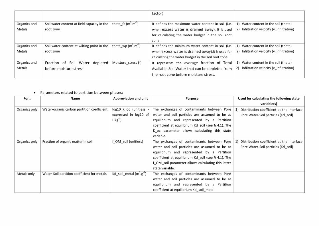
factor).
Organics and
Metals
Soil water content at field capacity in the
root zone
theta_fc (m3.m
-3) It defines the maximum water content in soil (i.e.
when excess water is drained away). It is used
for calculating the water budget in the soil root
zone.
1) Water content in the soil (theta)
2) Infiltration velocity (v_infiltration)
Organics and
Metals
Soil water content at wilting point in the
root zone
theta_wp (m3.m
-3) It defines the minimum water content in soil (i.e.
when excess water is drained away).It is used for
calculating the water budget in the soil root zone.
1) Water content in the soil (theta)
2) Infiltration velocity (v_infiltration)
Organics and
Metals
Fraction of Soil Water depleted
before moisture stress
Moisture_stress (-) It represents the average fraction of Total
Available Soil Water that can be depleted from
the root zone before moisture stress.
1) Water content in the soil (theta)
2) Infiltration velocity (v_infiltration)
Parameters related to partition between phases:
For… Name Abbreviation and unit Purpose Used for calculating the following state
variable(s)
Organics only Water-organic carbon partition coefficient log10_K_oc (unitless -
expressed in log10 of
L.kg-1
)
The exchanges of contaminants between Pore
water and soil particles are assumed to be at
equilibrium and represented by a Partition
coefficient at equilibrium Kd_soil (see § 4.1). The
K_oc parameter allows calculating this state
variable.
1) Distribution coefficient at the interface
Pore Water-Soil particles (Kd_soil)
Organics only Fraction of organic matter in soil f_OM_soil (unitless) The exchanges of contaminants between Pore
water and soil particles are assumed to be at
equilibrium and represented by a Partition
coefficient at equilibrium Kd_soil (see § 4.1). The
f_OM_soil parameter allows calculating this latter
state variable.
1) Distribution coefficient at the interface
Pore Water-Soil particles (Kd_soil)
Metals only Water-Soil partition coefficient for metals Kd_soil_metal (m3.g
-1) The exchanges of contaminants between Pore
water and soil particles are assumed to be at
equilibrium and represented by a Partition
coefficient at equilibrium Kd_soil_metal

Parameters related to diffusion between soil and atmosphere:
For… Name Abbreviation and unit Purpose Used for calculating the following state
variable(s)
Organics only Universal gas constant R
(=8.31 Pa.m3.mol
-1.K
-1)
Used to calculate the gaseous concentration of the substance in soil pore water that is assumed to be in equilibrium with the dissolved concentration.
1) Mass transfer coefficient in soil
porewater (MTC_porewater)
2) Overall Mass transfer coefficient in soil
(MTC_soil)
3) Overall Mass transfer coefficient at the
soil-atmosphere interface
(MTC_soil_atm)
Organics only Henry’s law constant H (Pa.m3.mol
-1) The gaseous concentration of the substance in soil
pore water is assumed to be in equilibrium with the dissolved concentration. This equilibrium is simulated by the adimensional Henry’s law constant.
1) Mass transfer coefficient in soil
porewater (MTC_porewater)
2) Overall Mass transfer coefficient in soil
(MTC_soil)
3) Overall Mass transfer coefficient at the
soil-atmosphere interface
(MTC_soil_atm)
Organics only Diffusion coefficient of water vapour in air D_H2O_air (m2.d
-1) The diffusion coefficient of the contaminant in
pure gas is assumed to be related to the diffusion
coefficient of water vapour in air.
1) Diffusion coefficient of the contaminant
in pure gas (D_gas_organic)
Organics only Diffusion coefficient of oxygen in water D_O2_water (m2.d
-1) The diffusion coefficient of the contaminant in
pure water is assumed to be related to the
diffusion coefficient of dioxygen in pure water.
1) Diffusion coefficient in pure water
(D_water_organic)
Organics only Molar mass of dioxygen M_O2 (g.mol-1
) The diffusion coefficient of the contaminant in
pure water is assumed to be related to the ratio
between the molar mass of the contaminant and
the molar mass of dioxygen
1) Effective diffusion coefficient in pure
water (D_water_organic)
Organics only Molar mass of water M_H2O (g.mol-1
) The diffusion coefficient of the contaminant in
pure gas is assumed to be related to the ratio
between the molar mass of H2O and the molar
mass of the contaminant
1) Effective diffusion coefficient in pure
gas (D_gas_organic)
Organics only Molar mass of the contaminant M_molar (g.mol-1
) The diffusion coefficient of the contaminant in
pure water is assumed to be related to the ratio
1) Effective diffusion coefficient in pure
water (D_water_organic)

between the molar mass of the contaminant and
the molar mass of dioxygen.
The diffusion coefficient of the contaminant in
pure gas is assumed to be related to the ratio
between the molar mass of H2O and the molar
mass of the contaminant.
2) Effective diffusion coefficient in pure
gas (D_gas_organic)
Organics only Boundary layer thickness in atmosphere
above the soil
Delta_atm (m) The mass transfer coefficient at the soil-
atmosphere interface is estimated according to
the assumption that it results from two
resistances in series. The Boundary layer thickness
in atmosphere above the soil corresponds to the
thickness where diffusion occurs in the
atmosphere at the soil-atmosphere interface.
1) Mass transfer coefficient in
atmosphere (MTC_atmosphere)
2) Mass transfer coefficient at soil-
atmosphere interface
(MTC_soil_atmosphere)
Parameters related to transport between soil layers:
Metals only Diffusion coefficient in water D_water_metal (m2.d
-1) The mass transfer coefficient between adjacent
soil layers is calculated from the effective
diffusivity in pure water
1) Mass transfer coefficient between
adjacent soil layers
Organics and
Metals
Bioturbation diffusion coefficient D_bioturbation (m2.d
-1) By analogy with diffusion in gas and water phases,
bioturbation is represented by a vertical Diffusion
coefficient D_bioturbation,. This D_bioturbation
coefficient applies exclusively to the contaminant
concentration on particles.
1) Mass transfer coefficient between
adjacent soil layers
Parameters related to transport from soil to rivers:
Organics and
Metals
Wash-off rate constant _washoff (d-1
) The wash-off rate constant has the inverse
dimension as the half-life, i.e. time needed to
reduce by a factor 2 the concentration of
chemicals in soils by both liquid and solid wash-
off

Parameters related to degradation:
For… Name Abbreviation and unit Purpose Used for calculating the following state
variable(s)
Organics only Global degradation rate in soil at 25°C lambda_deg_soil_25
(d)
Degradation of the chemical in soil is assumed to follow linear first-order kinetics. ‘lambda_deg_soil_25’ represents the degradation rate of the substance in soil at 25°C
1) lambda_deg_soil (d)
Organics only Factor of increase of degradation rate with an increase in temperature of 10°C (in brief: Degradation increase factor)
Q10 (-) Degradation of the chemical in soil is assumed to depend on temperature. Q10 represents the ratio between half-lives at 20°C and 10°C respectively
1) lambda_deg_soil (d)
3.8. Intermediate State variables
An ‘Intermediate State variable’ is defined as a dependent variable calculated within the model. Some State variables are fixed during a model run or
simulation because they are calculated only from parameters. Some others are time-dependent because they are calculated from parameters, but also from
time-dependent forcing variables. We distinguish ‘Intermediate State variables’ and ‘Regulatory State variables’. The first ones are generally not used by
decision-makers for regulatory purposes but can be used as performance indicators of the model that change over the simulation. The second ones can be
used by decision-makers for regulatory purposes.
For running the Soil model, the following state variables are calculated for the following purposes. All the state variables for which no forcing variable is
required are constant all over the calculation time. Instead, the state variables for which forcing variable(s) is/are required are time-dependent. In the
following tables, the following symbols were adopted:

Site-specific state variables:
For… State
variable n°
Name Abbreviation
and unit
Purpose Process followed for calculating the state variable
Organics
and Metals
1 Height of discretized soil
layer
h (m) The total soil horizon corresponding
to the root depth is subdivided in
sub-layers for the discretization of
the 1D general transport equation
including advection and diffusion
State variables related to partition between phases:
For… State
variable n°
Name Abbreviation
and unit
Purpose Process followed for calculating the state variable
Organics
only
2 Distribution coefficient at
the interface Pore
Water'-Soil particles
Kd_soil_organic
(m3.g
-1)
The exchanges of contaminants
between Pore Water and Soil
Particles are assumed to be at
equilibrium and represented by a
Partition coefficient at equilibrium
Kd_soil_organic.
State variables related to diffusion between soil and atmosphere:
For… State
variable n°
Name Abbreviation and
unit
Purpose Process followed for calculating the state variable

Organics
only
3 Effective diffusion
coefficient in pure
water
D_water_organic
(m2.d
-1)
The effective diffusion
coefficient of the
contaminant in pure water
can be estimated from the
effective diffusion
coefficient of O2 in pure
water
Organics
only
4 Effective diffusion
coefficient in pure
gas
D_gas_organic
(m2.d
-1)
The effective diffusion
coefficient of the
contaminant in pure gas
can be estimated from the
effective diffusion
coefficient of H2O in pure
gas
Organics
only
5 Mass transfer
coefficient in soil
porewater
MTC_porewater
(m.d-1
)
The mass transfer
coefficient in water-filled
pore space is assumed to
depend on the diffusion
coefficient in pure water
corrected by a tortuosity
factor (that depends on
water content in soil) and
partition between water
and gas in pore soil space.
Organic
only
6 Mass transfer
coefficient in soil
pore air
MTC_pore_air
(m.d-1
)
The mass transfer
coefficient in air-filled pore
space is assumed to
depend on the diffusion
coefficient in pure gas
corrected by a tortuosity
factor (that depends on gas
content in soil, i.e. the
difference between the

maximum water content fc
and the actual water
content.
Organic
only
7 Overall Mass
transfer coefficient
in soil
MTC_soil (m.d-1
) The overall mass transfer
coefficient in soil results
from two resistances in
derivation, i.e. the mass
transfer coefficient in
water-filled pore space
MTC_porewater and the
mass transfer coefficient in
air-filled pore space
MTC_pore_air
Organic
only
8 Mass transfer
coefficient in
atmosphere
MTC_atm (m.d-1
) The mass transfer
coefficient in atmosphere
above soil is assumed to
depend on the diffusion
coefficient in pure gas and
on the film layer thickness.
Organic
only
9 Overall Mass
transfer coefficient
at the soil-
MTC_soil_atm
(m.d-1
)
The overall mass transfer
coefficient at the soil-
atmosphere interface

atmosphere
interface
results from two
resistances in series, i.e. the
overall mass transfer
coefficient in soil MTC_soil
and the mass transfer
coefficient in atmosphere
MTC_atm
State variables related to water mass balance in soil and infiltration:
For… State
variable n°
Name Abbreviation and
unit
Purpose Process followed for calculating the state variable
Organics
and
Metals
10 Soil water content
at no stress point
in the root zone
theta_no_stress
(m3.m
-3)
It is used for calculating the
water budget in the soil root
zone. It defines the soil water
content that a crop can extract
from the root zone without
suffering water stress (readily
available soil water)..
Organics
and
Metals
11 Global solar
radiation
Ig (cal.cm-2
.s-1
) Evapotranspiration is assumed
to depend on global solar
radiation. Global solar radiation
is derived from a maximum
value corrected by sunshine
duration and daylight duration.

Organics
and
Metals
12 Potential
evapotranspiratio
n
ETp (mm.d-1
) Evapotranspiration is a loss of
water from soil and is then
taken into account for
calculating water content in
soil. Potential
evapotranspiration represents
evapotranspiration on bare soil.
Organics
and
Metals
13 Actual
evapotranspiratio
n
ETa (mm.d-1
) Evapotranspiration is a loss of
water from soil and is then
taken into account for
calculating water content in
soil. Actual evapotranspiration
represents evapotranspiration
on cultivated soil.

Organics
and
Metals
14 Advection
velocity
v_adv (m.d-1
) Advection is assumed to occur
at a velocity v_adv when water
content exceeds water content
at field capacity.
Organics
and
Metals
15 Net water budget
in soil
_water_budget (d-1
) The Water budget in soil
calculates the net budget
between water inputs (rainfall,
groundwater contribution,
irrigation) and water outputs
(evapotranspiration,
percolation) to/from soil
Organics
and
16 Soil water content
in the root zone
Theta (m3.m
-3) It defines the soil water content
in the root zone. It is used for
Calculated from the mass balance equation of water in soil, accounting for inputs from rainfall
and irrigation, and outputs from evapotranspiration and percolation (see 7.1)

Metals calculating the advection
velocity of water and
chemicals.
State variables related to diffusion within soil:
For… State
variable n°
Name Abbreviation
and unit
Purpose Process followed for calculating the state variable
Organics
and Metals
17 Retardation factor f_retardation
(-)
The contaminant is partly sorbed
on the solid phase, only the
dissolved phase is assumed to
move along the depth profile,
resulting in a retardation factor.
The Retardation factor
incorporates the adsorption of
contaminants on the particulate
soil phase and is included in the
advection-diffusion transport
equation within the soil profile.
Organics
and Metals
18 Effective diffusion in
soil
D_soil (m2.d
-1) The fate of the chemical within the
soil column because of diffusion
process is described by 1D general
transport equation. D_soil
represents the effective diffusion
coefficient applicable for the total
concentration in soil and is a
combination of diffusion
coefficients in water, gas and
solids (bioturbation).
State variables related to degradation:

For… State
variable n°
Name Abbreviation and unit Purpose Process followed for calculating the state variable
Organics
only
19 Global
degradation
rate in soil
lambda_deg_soil (d) Degradation of the chemical in soil is assumed to follow a linear first-order kinetics and to depend on temperature
3.9. Regulatory State variables
An ‘Regulatory State variable’ is defined as a dependent variable calculated within the model. It is generally time-dependent because it is calculated from
parameters, but also from time-dependent forcing variables and loadings. We distinguish ‘Intermediate State variables’ and ‘Regulatory State variables’. The
first ones are generally not used by decision-makers for regulatory purposes but can be used as performance indicators of the model that change over the
simulation. The second ones can be used by decision-makers for regulatory purposes.
Following pages:
Figure 12 - Flow chart for calculating the ‘regulatory state variables’ (for Organics)
Figure 13 - Flow chart for calculating the ‘regulatory state variables’ (for Metals)


The following ‘regulatory state variables’ are calculated according to the flow charts presented in
and Figure 13Figure 13:
State variable n° Name Abbreviation and unit
20 Total concentration of the chemical in soil surface C_tot_topsoil (mg.kg-1
)
21 Dissolved concentration of the chemical in soil surface C_dis_topsoil (mg.m-3
)
22 Total concentration of the chemical in deep soil C_tot_deep_soil (mg.kg-1
)
23 Dissolved concentration of the chemical in deep soil C_dis_deep_soil (mg.m-3
)
24 Total concentration of the chemical in the root zone
averaged over depth
C_tot_root_zone (mg.kg-1
)
25 Dissolved concentration of the chemical in the root zone
averaged over depth
C_dis_root_zone (mg.m-3
)
End of Level 1 documentation (basic end-user)

38
Level 2 documentation (background science)
4. Processes and assumptions
4.1. Process n°1: Sorption/desorption between Pore water and Soil
particles Motivation
Exchanges of contaminants between the dissolved (i.e. porewater) and the particulate phases of soil
govern their flux towards atmosphere and deeper soil layers because: (i) only dissolved contaminants
can exchange by diffusion (except bioturbation – see 4.6) between two successive soil layers along
the vertical axis; (ii) only dissolved contaminants can move by advection towards deeper soil layers
together with water advective movement; (iii) only gaseous contaminants, which are assumed to be
in equilibrium with the dissolved phase, can exchange by diffusion at the Soil-Atmosphere interface.
Selected model and assumptions
Exchanges of contaminants between porewater and soil particles are assumed to be equilibrated,
and thus described by a distribution (or partition) coefficient Kd_soil (see § 5.2.3), expressed as the
concentration ratio between the particulate phase and the dissolved phase respectively. For organic
pollutants, exchanges are governed by a hydrophobic sorption mechanism and the distribution
coefficient Kd_soil_organic is related to the octanol-water partition coefficient Koc (see § 5.2.3.1),
and the concentration of organic matter in the soil particles f_OM_soil (see § 5.2.3.2).
Model type
Empirical [X] vs mechanistic [ ]
Steady-state [X] vs dynamic [ ]
Analytical [X] vs numerical [ ]
Alternatives and limits
When equilibrium condition between porewater and soil particles is not respected, e.g. just after a
direct application, the model must then be considered with cautious. In such a case, exchanges
between water and SPM should be described by non equilibrium kinetics, using sorption and
desorption kinetic rate constants.
4.2. Process n°2: Evapotranspiration Motivation
The vertical movement of pore water in soils leads to downward infiltration (drainage) of dissolved
contaminants. To calculate such water movement, it is necessary to calculate water mass balance in
soil, accounting for all the inputs (rainfall, irrigation) and outputs (evapotranspiration, infiltration).
Evapotranspiration is a water upward flux loss term and is dynamically calculated according to
meteorological conditions.
Selected model and assumptions
The actual evapotranspiration ETa may be estimated by taking into account the potential
evapotranspiration ETp and a time-dependent cultural coefficient K_cultural that may be lower or
higher to unity according to the stage of development of the plant.

39
To calculate a monthly average estimation of potential evapotranspiration ETp, the 4FUN model uses
the Turc’s relationship that uses as variables the mean air temperature and the global solar radiation.
Model type
Empirical [X] vs mechanistic [ ]
Steady-state [ ] vs dynamic [X]
Analytical [X] vs numerical [ ]
Alternatives and limits
Other evapotranspiration models are available in the literature, including more sophisticated models.
For example, the Penman–Monteith or Penman-FAO models calculate potential evapotranspiration
from several variables, e.g. the latent heat of vaporization; volumetric latent heat of vaporization;
rate of change of saturation specific humidity with air temperature; net irradiance; ground heat flux;
specific heat capacity of air; dry air density, vapor pressure deficit, or specific humidity, Conductivity
of air, Conductivity of stoma, Psychrometric constant. All these variables are difficult to measure and
are poorly available. A simpler model based on two accessible variables was then preferred. It must
however be noted that the chosen Turc’s equation provides an estimation of evapotranspiration at a
monthly time scale and not at a daily scale.
4.3. Process n°3: Water mass balance in soil and loss by infiltration Motivation
The vertical movement of pore water in soils leads to downward infiltration (drainage) of dissolved
contaminants that thus reach deeper soil layers. In many models, a constant advection velocity is
considered, whatever meteorological and soil conditions. The downward infiltration of water in soil is
however highly variable because it depends on soil moisture. In the 4FUN model, a time-dependent
advection velocity was determined from water dynamics in the soil profile.
Selected model and assumptions
Water mass balance in soil is assumed to be governed by the following processes: rainfall, irrigation,
evapotranspiration and infiltration water flux. Rainfall and irrigation are inputs of water to soil;
evapotranspiration is a upward flux loss term; infiltration is a downward flux loss term. Water
content in soil is dynamically calculated from the mass balance resulting from these input/loss
contributions.
In order to calculate the quantity of water infiltrating to deeper soil layers (i.e. to calculate the
Infiltration velocity v_adv), the water storage in soil (over the investigated depth) is subdivided into
three different fractions (Figure 14Figure 14) : (i) the excess water fraction, corresponding to
gravitational water and corresponding to the fraction exceeding ‘Water content at field capacity’
(theta_fc). ‘Water content at field capacity’ is indeed defined as the amount of soil water content
held in the soil after excess water has drained away. It can be assimilated to the maximum water
content in soil; (ii) the “optimal yield‟ fraction, where water is readily available by plants to reach
maximal yields, and corresponding to water content between ‘Water content at no stress’
(theta_no_stress) and ‘Water content at field capacity’ (theta_fc). In dry soils, the water has a low
potential energy and is strongly bound by capillary and absorptive forces to the soil matrix, and is less
easily extracted by the crop. When the potential energy of the soil water drops below a threshold

40
value, the crop is said to be water stressed. The threshold value corresponds to the ‘soil water
content at no stress point’ that is a state variable calculated from Soil water content at field capacity
and Soil water content at wilting point; (iii) the water stress fraction, where water is low enough to
induce plant stress, and corresponding to water content between ‘water content at wilting point’
(theta_wp) and ‘Water content at no stress’ (theta_no_stress); ‘water content at wilting point’ is
indeed defined as the minimal point of soil moisture the plant requires not to wilt.
According to actual water content, different processes can be initiated: (i) downward water flux (i.e.
infiltration) occurs only for excess water, i.e. for the fraction exceeding field capacity; (ii) if water
content is in the water stress zone, evapotranspiration is limited.
Figure 14 – Schematic representation of the different fractions of water storage in soil
Model type
Empirical [ ] vs mechanistic [X]
Steady-state [ ] vs dynamic [X]
Analytical [X] vs numerical [ ]
Alternatives and limits
Many ‘soil water’ models are available in the literature (see for example Ranatunga et al, 2008). They
differ by the complexity of the spatial description of the soil compartment (e.g. single vs multiple
layer models), the incorporation of groundwater component or not, the incorporation of runoff
processes or not, etc. But, they are all based on a water balance estimation accounting for the main
inputs (rainfall) and outputs (evapotranspiration, drainage). To refine the 4FUN model, other
secondary components in the water balance (groundwater contribution, runoff) could be included.
4.4. Process n°4: Retardation factor and advection within soil Motivation
The water infiltration velocity is calculated according to the assumptions and process described in
4.3. However, because the contaminant is partly sorbed on the solid phase, only the dissolved phase
is assumed to move along the depth profile, resulting in a retardation factor. In other words, the
Retardation factor incorporates the adsorption of contaminants on the particulate soil phase and is
included in the advection transport equation within the soil profile. Assuming that the partitioning of
the contaminant is described with a linear isotherm, the retardation factor f_retardation is a
dimensionless parameter defined as the amount by which a chemical is held back by the soil in
comparison to the water velocity. In other words, how much the flow of the contaminant is retarded
as compared to flow of the infiltrating water.

41
Selected model and assumptions
The fate of the chemical within the soil column because of advection process can be described by 1D
general transport equation. Because advection (or infiltration) applies only to the dissolved phase,
the transport equation is under the form:
z
Cv
t
C Wadv
T
where CT is the total soil concentration (g.m-3), CW is the concentration in pore soil water (in g.m-3
water), z is the soil depth (m), vadv is the advection velocity (m.d-1).
This equation can be solved without previous modification because both the total and dissolved
concentrations are involved. To homogenize the equation, total soil concentration is expressed as
the sum of the three phase concentrations:
SGWT CaCCC
where CG and CS are the concentrations in gas and solids of the soil (in g.m-3 air and g.kg-1), θ (m3
water.m-3soil) is the volumetric water content ; a (m3air.m-3soil) the volumetric air content.
Considering that water, gaseous and solid phases are assumed to be in equilibrium, i.e.:
W
SOCOCD
C
CKyK and
W
GAW
C
C
RT
HK
where KD (m3.kg-1) is the ratio between particulate and porewater contamination, H is the Henry’s
law constant (Pa.m3.mol-1), R the universal gas constant (Pa.m3.mol-1.K-1) and T the temperature at
the soil-air interface (K).
Combining these equations, the first Equation can be rewritten:
z
Cv
t
C Te
T
where ve is the effective advection velocity (m.d-1)
nretardatiof
vv adv
e_
,
and f_retardation (unitless) is the water phase retardation factor
AWD aKKnretardatiof _
The Retardation factor can thus be calculated from soil properties (bulk density, water content and
air content) and chemical partition coefficient (air-water partition coefficient). This equation is
rewritten in Part 3 with the 4FUN abbreviations.
Model type
Empirical [ ] vs mechanistic [X]
Steady-state [ ] vs dynamic [X]

42
Analytical [ ] vs numerical [X]
Alternatives and limits
In some publications, another formulation of the Retardation factor can be found under the form
DKnretardatiof 1_ . In this case however, the air content is not taken into account while it
can be important for some organic substances.
4.5. Process n°5: Diffusion between soil and atmosphere (only for
Organics) Motivation
Some pollutants that are highly volatile (or Semi Volatile Organic Compounds – SVOCs) can be
emitted from soil surfaces and the transfer from soil to atmosphere can be a significant contribution
to the mass balance of the chemical in soil.
Selected model and assumptions
Absorption/volatilization of semi-volatile substances at the air-soil interface is modelled using the
stagnant boundary theory (two-film model), the pollutant being assumed to diffuse across two layers
(stagnant soil layer and stagnant air layer) characterized by two resistances in series (the soil
resistance resulting itself of the combination of two resistances in parallel) (Figure 15Figure 15).
According to this approach, the net flux from soil to the atmosphere is driven by the difference in
gaseous concentration between air and surface soil according to the Fick’s law.
The gaseous concentration of the substance in soil porewater is assumed to be in equilibrium with
the dissolved concentration. This equilibrium is simulated by the adimensional Henry’s law constant.
The first resistance represents the resistance to diffusion on the upper part of the interface (i.e. in
the thin boundary layer in atmosphere over the soil surface). A ‘Mass transfer coefficient in
Atmosphere’ (noted MTC_atmoshere) is thus calculated by dividing the diffusion coefficient of the
contaminant in air (D_gas_organic) by the boundary layer thickness in atmosphere (Delta_atm).
In the soil, two resistances are involved in parallel, representing diffusion within the soil in either
water-filled pore space or air-filled pore space. These two resistances are described by two
parameters: the mass transfer coefficient in soil porewater (MTC_porewater) and the mass transfer
coefficient in soil pore air (MTC_pore_air). These coefficients are estimated as described by
Millington et Quirk (1961), taking into account a tortuosity factor limiting diffusion in soil. The
boundary layer thickness in soil (corresponding to the thickness where diffusion occurs within the
soil at the soil-atmosphere interface) is assumed to correspond to the thickness of the first soil layer.

43
Figure 15 – Conceptual representation of resistances involved in diffusion process at the Soil-Atmosphere
interface
Model type
Empirical [ ] vs mechanistic [X]
Steady-state [ ] vs dynamic [X]
Analytical [X] vs numerical [ ]
Alternatives and limits
Other combinations of resistances were proposed in the literature. Thus, the deposition to the
surface can be assumed to be controlled by three resistances in series (aerodynamic, quasi-laminar
layer and surface resistances). A deposition velocity is thus computed from these three resistances
and allows calculating dry deposition of gaseous pollutants (Wesely, 2000). The fugacity approach
selected in the 4FUN model was however chosen because it offers the advantage of taking into
account both deposition and volatilization of gaseous pollutants.
4.6. Process n°6: Bioturbation Motivation
Bioturbation refers to the disturbance of soil layers by biological activity. Some species (e.g.
earthworms) disturb the soil by burrowing and feeding, enhancing the transport of chemicals in this
compartment. Animals move indeed through the soil to obtain nutrients and water, or to seek
protection from predators or environmental variability. In doing so, they penetrate the soil vertically
and horizontally. Bioturbation was showed to be a significant soil mixing vertical process in many
situations (Müller-Lemans et Van Dorp, 1996, Farenhorst et al, 2000).
Bioturbation can thus be seen as the process that is responsible for the sorbed phase transport of
chemicals in soil depth. Vertical sorbed phase transport in the soil was shown to have a major impact
on predicted air and soil concentrations, the state of equilibrium, and the direction and magnitude of
the chemical flux between air and soil. It is a key process influencing the environmental fate of
persistent organic pollutants (POPs).
Selected model and assumptions
McLachlan et al (2002) and Cousins et al (1999) suggested incorporating the bioturbation process as
an additional diffusion process, representing the vertical sorbed phase transport. This process was
then assimilated to a diffusion component in the solid phase. By analogy with diffusion in gas and
water phases, bioturbation is represented by a vertical Diffusion coefficient D_bioturbation,

44
expressed in m2.d-1. This D_bioturbation coefficient applies exclusively to the contaminant
concentration on particles.
Model type
Empirical [ ] vs mechanistic [X]
Steady-state [ ] vs dynamic [X]
Analytical [X] vs numerical [ ]
Alternatives and limits
To our knowledge, no other model was developed for studying the bioturbation rates of pollutants in
soils.
4.7. Process n°7: Diffusion within soil Motivation
Diffusion within soil (i.e. here between adjacent soil layers) is governed by the general 1D transport
model, and is directed according to the concentration gradient within soil (Fick’s law). Diffusion
occurs in the three soil phases: (i) bioturbation leading to particles turnover over soil depth is
assimilated to a diffusion process and described by a Bioturbation diffusion coefficient (see 4.6); (ii)
as far as processes occurring in water and gas in a porous media like soil, diffusion differs from
diffusion in free water and pure gas. Effective diffusion coefficients are then defined from diffusion
coefficient in pure phases corrected by a tortuosity factor to account for the reduced flow area and
increased path length of diffusing gas and water molecules in soil. This tortuosity factor is a function
of volumetric air content (respectively water content for diffusion coefficient in water phase) and of
soil geometry. One model that has proven useful for describing pesticide soil diffusion coefficients is
the Millington-Quirk model (reported in Jury et al, 1983).
Besides, because the contaminant is partly sorbed on the solid phase, only a fraction of the
contaminant is subject to diffusion in water and gas along the depth profile, resulting in a retardation
factor. The Retardation factor incorporates the adsorption of contaminants on the particulate soil
phase and is included in the diffusion transport equation within the soil profile. Assuming that the
partitioning of the contaminant is described with a linear isotherm, the retardation factor
f_retardation is a dimensionless parameter that measures how much diffusion of the contaminant is
retarded as compared to what would occur without sorption.
Selected model and assumptions
The fate of the chemical within the soil column because of diffusion process can be described by 1D
general transport equation. Because diffusion coefficients are different for the gaseous, dissolved
and particulate forms of the chemical, the transport equation is under the form:
2
2
2
2
2
2
.z
CD
z
CD
z
CD
t
C Ss
WW
GG
T
where CT is the total soil concentration (g.m-3), CG, CW and CS are the concentrations in gas, water and
solids of the soil (in g.m-3 air, g.m-3 water and g.kg-1), z is the soil depth (m),; DG and DW (m2.d-1) are

45
the diffusion coefficients in gaseous and liquid phases; DS (m2.d-1) is the vertical bioturbation
coefficient (see 4.6), ρ is the soil density (kg.m-3).
This equation can be solved without previous modification because both the total, dissolved, gaseous
and particulate concentrations are involved. To homogenize the equation, total soil concentration is
expressed as the sum of the three phase concentrations:
SGWT CaCCC
where θ (m3 water.m-3soil) is the volumetric water content ; a (m3air.m-3soil) the volumetric air
content.
Considering that water, gaseous and solid phases are assumed to be in equilibrium, i.e.:
W
SOCOCD
C
CKyK and
W
GAW
C
C
RT
HK
where KD (m3.kg-1) is the ratio between particulate and porewater contamination, H is the Henry’s
law constant (Pa.m3.mol-1), R the universal gas constant (Pa.m3.mol-1.K-1) and T the temperature at
the soil-air interface (K).
Combining these equations, the first Equation can be rewritten:
2
2
z
CD
t
C Tsoil
T
where DT is the effective diffusion coefficient (m2.d-1).
nretardatiof
DKDDKD SDWGAW
soil_
,
and f_retardation (unitless) is the retardation factor
AWD aKKnretardatiof _
The Retardation factor is identical to those calculated for advection (see 4.4) and can thus be
calculated from soil properties (bulk density, water content and air content) and chemical partition
coefficient (air-water partition coefficient). This equation is rewritten in Part 3 with the 4FUN
abbreviations.
Model type
Empirical [ ] vs mechanistic [X]
Steady-state [ ] vs dynamic [X]
Analytical [ ] vs numerical [X]
Alternatives and limits
In some publications, another formulation of the Retardation factor can be found under the form
DKnretardatiof 1_ . In this case however, the transport equation have to be applied to the

46
solute phase only and the air content is not taken into account while it can be important for some
organic substances.
4.8. Process n°8: Wash-off from soils to river Motivation
Pollutant „wash-off‟ designates the transport of contaminants in water flowing over the soil surface
and finally reaching freshwater systems (rivers and/or lakes). It includes runoff of dissolved
contaminants and erosion of contaminated soil particles. Wash-off from watersheds is a loss process
from soils and can be a significant secondary input into freshwaters because these latter collect
water and particle fluxes from potentially wide areas, especially during rainfall.
Selected model and assumptions
The approach selected in the 4FUN model is based on global wash-off rate constants directly relating
concentrations in soils and inputs into rivers. Such global rate constants were fitted especially in the
field of radioecology. They were calibrated using datasets collected after the Chernobyl accident for a
wide range of European rivers; the Chernobyl accident corresponds indeed to a single atmospheric
pulse with well-known spatial mapping of soil contamination and follow-up of rivers contamination
during short and long periods after the deposit, allowing to fit global transfer functions from
watersheds to freshwater systems (Garcia-Sanchez et al, 2008).
Model type
Empirical [X] vs mechanistic [ ]
Steady-state [ ] vs dynamic [X]
Analytical [X] vs numerical [ ]
Alternatives and limits
Some models consider also transfer functions, but directly from rainwater to freshwaters, shunting
thus the soil system. For example, the SimpleBox multimedia model assumed that a constant
proportion of rainwater directly reaches freshwater systems and that this fraction is in immediate
equilibrium with soil (same concentration and same partition between water and particles, described
by the soil distribution coefficient). Thus, SimpleBox directly connects rainwater to freshwater
through a constant transfer rate and shunts many processes actually occurring in natural soil
systems.
Other empirical models take into account short kinetic and spatial variations in the rainfall regime to
simulate the loss of runoff water from soil during a given meteorological event. For example, the
PRZM multimedia model incorporated the “SCS runoff curve number approach” developed by USGS
(USDA, 1986). This approach calculates the soil depth impacted by runoff according to the rainfall
event and to an empirical parameter (called „curve number‟) implicitly accounting for landscape
characteristics (like hydrologic soil group, slope of the field and land use coverage). This approach is
mechanistically relevant because wash-off is indeed by nature intermittent as it is related to the
rainfall regime: it increases after heavy rainfall, floods and snowmelt. Besides, it can show high
spatial variability, even at small scales, because it depends on the slope of the field and on its cover.
However, this approach is essentially used at a local scale (rather than at a watershed scale) to
predict the loss of water, particles and eventually associated contaminants from a field; it requires

47
several information related to slope and land use of the field. A more global approach was then
preferred in the 4FUN tool.
4.9. Process n°9: Degradation (only for Organics) Motivation
Degradation can be a significant loss term in soils.
Selected model and assumptions
The individual processes that are responsible for degradation (e.g. biodegradation, photolysis,
hydrolysis) are not distinguished here but they are added into an aggregated loss rate. Degradation is
assumed to to follow linear first-order kinetics.
Temperature is assumed to be one of the main factors influencing the degradation rate of chemicals. A possible approach for relating the half-life of a given substance and temperature is to introduce a coefficient, generally noted Q10, which represents the ratio between the rates at 20° and 10°C. This approach is those generally used for Plant Protection Products (EFSA, 2007).
Model type
Empirical [X] vs mechanistic [ ]
Steady-state [X] vs dynamic [X]
Analytical [X] vs numerical [ ]
Alternatives and limits
Degradation processes are generally simulated by pseudo first order degradation rates (i.e.
degradation proportional to the concentration of contaminants in the media). However,
transformation processes can distinguish the following mechanistic processes: (i) hydrolysis (acid-
and base-catalyzed hydrolysis can be modelled according a thermodynamic principle); (ii) photolysis
(that should involve light intensity); (iii) microbial degradation (that can be calculated by a maximum
microbial degradation rate, eventually attenuated by anaerobic conditions, suboptimal temperature
and suboptimal pH). Such processes are considered individually in some specific models. However,
such an approach requires a lot of parameters that are poorly available for most of the chemicals and
a global loss rate was preferred.
The effect of temperature on degradation can also be described by the Arrhenius equation which
gives the degradation rate coefficient as a function of the temperature and the activation energy Ea.
This approach requires the determination of the activation energy Ea for each substance.
End of Level 2 documentation (end-user with expertise in
process)

48
Level 3 documentation (numerical information)
5. Numerical default values (deterministic and/or probabilistic)
5.1. Initialization of concentrations in Media The ‘regulatory state variables’, i.e. the concentrations of the chemical in soil (i.e. the total
concentration in soil surface C_tot_topsoil_0 (mg.kg-1 dw), the total concentration in soil layers i
C_tot_deep_soil_0 (mg.kg-1 dw) must be initialized (i.e. value for time=0). By default, no
contamination is assumed at the beginning of the simulation, i.e. all the concentrations are put at
zero, but end-user must adapt these values according to their specific case studies (e.g. initial
contamination in sediments).
The water content in soil (i.e. tetha_0) must also be initialized (i.e. value for time=0). By default,
tetha_0 is assuled to be 0.2 at the beginning of the simulation (intermediate level between wilting
point and field capacity), but this value can be changed by the end-user.
5.2. Default parameter values
5.2.1 Site-specific parameters
5.2.1.1 Soil surface
Physical/chemical/biological/empirical meaning
The Surface of the soil zone under investigation (S_field) represents the dimensions of the region
under evaluation. The relevant spatial scale is governed by the homogeneity of the soil system under
investigation (e.g. homogeneity in contamination levels, agricultural practices, mineralogical
properties, meteorological conditions). It is advised to define a soil surface that show low variations
in its land use.
Factors influencing parameter value
Parameter values are purely site-specific.
Role in the model
Soil surface is used for converting the total mass in the system into concentrations in soil (final state
variable of interest).
Database used for parameter estimation
Not applicable
Parameter values are purely site-specific and must be informed by the end-user case by case.
Parameter estimation type
Statistical analysis of large database [ ]
Calibration [ ]
Extrapolation [ ]
Expert elicitation [ ]

49
Bayesian approach [ ], eventually
QSAR or read-across [ ]
Mechanistic model [ ]
Perfect information [X] to be informed by the end user case by case
Parameter estimation description
Not applicable
Parameter default value and PDF
Because they are purely site-specific, no default best estimate and PDF are provided here.
5.2.1.2 Depth of the root zone
Physical/chemical/biological/empirical meaning
The depth of the root zone represents the depth of the soil over which the distribution of the
contaminant is estimated. When coupled to a Plant model (Root, Tuber, Leaf, Grass, Fruit and
Cereal), it is reliable to define the depth of the investigated soil as the depth of the root zone.
Factors influencing parameter value
The depth of the root zone depends by nature on the plant under investigation and on the soil type.
Role in the model
The depth of the root zone is used for calculating the water budget in the soil root zone. It defines
the soil depth where the contaminant mass balance is calculated.
Database used for parameter estimation
Breuer et al (2003) conducted a comprehensive review of several parameters relevant for plant
description, including values for the root depth. Some of the values collected in this review are
reported in Table 1Table 1. These values can be used for defining the depth of the root zone
according to the crop under investigation.
Latin name Common name Number of references
Range (in m)
Avena sativa Oat 7 0.6-2.5
Beta vulgaris Beet 2 0.9-1.1
Brassica napus Colza 8 0.85-1.75
Helianthus annuus Sunflower 3 1.6-2.75
Hordeum distichum/ Hordeum vulgare Barley 9 0.8-2.6
Medicago sativa Alfalfa 7 1.3-3.8
Pisum sativum Garden pea 2 0.7-1.5
Secale sereale Rye 12 0.75-2.3
Solanum tuberosum Potato 6 0.8-2.2
Triticum aestivum Wheat 18 0.5-2.8
Zea mays Corn 3 0.9-2.4
Herb, grasses 42 0.1-2.1
Table 1 – Ranges of root depths collected by Breuer et al (2003) for different crops

50
FAO (Food Agriculture Organization) proposes soil root depths ranges for a variety of vegetables
(http://www.fao.org/docrep/x0490e/x0490e0e.htm#TopOfPage).These values can also be used for
defining the depth of the root zone according to the crop under investigation.
Crop Range (m)
Broccoli 0.4-0.6
Brussel Sprouts 0.4-0.6
Cabbage 0.5-0.8
Carrots 0.5-1.0
Cauliflower 0.4-0.7
Celery 0.3-0.5
Garlic 0.3-0.5
Lettuce 0.3-0.5
Onions 0.3-0.6
Spinach 0.3-0.5
Radishes 0.3-0.5
Fruit trees: apples, pears, cherries, apricots, peaches, grapes
1.0-2.0
Fruit trees: kiwi 0.7-1.3
Citrus 0.8-1.5
Olives 1.2-1.7
Table 2 - Ranges of root depths proposed by FAO for different crops
Parameter estimation type
Statistical analysis of large database [X]
Calibration [ ]
Extrapolation [ ]
Expert elicitation [X]
Bayesian approach [ ], eventually
QSAR or read-across [ ]
Mechanistic model [ ]
Perfect information [ ] to be informed by the end user case by case
Parameter estimation description
The range of the root zone depth can be chosen according to the values proposed in Table 1Table 1.
Parameter default value and PDF
Best estimates and PDF can be taken from Table 1Table 1 and uniform distributions can be chosen.
As default value in the MERLIN-Expo model, the value h_root=0.5 m is proposed. It can be changed
according the type of plant that is investigated.
5.2.1.3 Number of soil layers
Physical/chemical/biological/empirical meaning
The depth of the root zone is subdivided in several soil layers. These layers are used in the
discretization of the general 1D transport model in soil including advection and diffusion.

51
Factors influencing parameter value
Parameter value depends on level of precision chosen by the end-user.
Role in the model
See above
Database used for parameter estimation
Not applicable
Parameter values are purely site-specific and must be informed by the end-user case by case.
Parameter estimation type
Statistical analysis of large database [ ]
Calibration [ ]
Extrapolation [ ]
Expert elicitation [ ]
Bayesian approach [ ], eventually
QSAR or read-across [ ]
Mechanistic model [ ]
Perfect information [X] to be informed by the end user case by case
Parameter estimation description
The number of soil layers is defined by the end-user according to the level of precision that is expected as well as to site-specific conditions. It must however be highlighted that the number and depth of the soil layers is important because they define the volumes in which pollutants are diluted, and they are thus sensitive parameters for the calculation of the contaminant redistribution in soil. It was in particular demonstrated that a compartmental model can provide valid results only if a minimum number of compartments is set to a specific value determined by the advection/diffusion flow conditions. For example, Kirchner (1998) calculated the minimal number of compartments to be included for a proper description of soil, in different flow conditions; as an example, for convection-
dominated flow, D
hVN
2
. , where N is the number of compartments, v the pore water advection
velocity, h the total soil depth and D the diffusion coefficient. Similar relationships can be found in other compartmental models described in Basagaoglu et al (2002), Bidwell (1999) or Sardin et al (1991).
Parameter default value and PDF
Because they are purely site-specific, no default best estimate and PDF are provided here.
5.2.2 Soil physico-chemical properties of soil
5.2.2.1 Dry density of soil
Physical/chemical/biological/empirical meaning
The dry density of soil represents the mass of soil particles per unit volume of soil.
Factors influencing parameter value
The soil density is influenced by soil type (e.g. loam, silt, sand, organic soils).
Role in the model

52
The dry density of soil is a parameter involved in the calculation of the retardation factor of
contaminants in soil (see 4.4).
Database used for parameter estimation
Baes and Sharp (1984) reviewed a lot of values obtained on soil from different textures and proposed
mean and extreme values for five different textures (Table 3Table 3).
Soil texture Number of soils analysed
Mean Observed range
Silt loams 99 1330 860-1670
Clay and clay loams 49 1300 940-1540
Sandy loams 37 1500 1250-1760
Gravelly silt loams 15 1220 1020-1420
Loams 22 1420 1160-1580
All soils 222 1350 860-1760
Table 3 – Mean and range of soil density collected by Baes and Sharp (1984) for different soil textures
Parameter estimation type
Statistical analysis of large database [X]
Calibration [ ]
Extrapolation [ ]
Expert elicitation [ ]
Bayesian approach [ ], eventually
QSAR or read-across [ ]
Mechanistic model [ ]
Perfect information [X] to be informed by the end user case by case
Parameter estimation description
Parameter estimation is based on the ranges proposed by Baes et sharp (1984).
Parameter default value and PDF
When no specific information is known about the soil texture, generic best estimate and PDF are
proposed. A uniform distribution is chosen according to the range observed by Baes et Sharp (1984).
Best estimate(rho_soil_dry) = 1350 kg dw.m-3
PDF(rho_soil_dry) = U(min=860 ; max=1760) kg dw.m-3
5.2.2.2 Soil water content at field capacity
and
5.2.2.3 Soil water content at wilting point
Physical/chemical/biological/empirical meaning
‘Soil water content at field capacity’ is the amount of soil water content held in the soil after excess
water has drained away. It can be assimilated to the maximum water content in soil.

53
‘Soil water content at wilting point’ is defined as the minimal point of soil moisture the plant requires
not to wilt. A physical definition is also possible, i.e. the wilting point is defined as the water content
at −1500 J/kg of suction pressure, or negative hydraulic head. In the 4FUN model, it is assimilated to
the minimum water content in soil.
Factors influencing parameter value
Several pedotransfer functions were developed to predict soil water contents at field capacity and
wilting point from soil physical properties. A review is proposed in Donatelli (2004) and the variables
used for predicting soil water contents in several pedotransfer functions are reported in Table 4Table
4. These latter show that the water content thresholds can be influenced by soil texture (clay, silt,
sand content), organic matter and/or bulk density.
Pedotransfer function Variables used for calculating soil water contents at field capacity
and wilting point
Brakensiek-Rawls Sand content, Clay content, Organic Matter content, Bulk density
Hutson Clay content, Silt content
British soil service Clay content, Silt content, Organic Matter content, Bulk density
Baumer Sand content, Clay content, Cationic Exchange Capacity (CEC), Bulk
density
Manrique Sand content, Clay content, Bulk density
Table 4 – Variables used in several pedotransfer functions for calculating water contents at field capacity and
wilting point
Role in the model
The water contents at field capacity, at wilting point are used for calculating the water budget in the
soil root zone (see 4.3).
Database used for parameter estimation
Baes and Sharp (1984) reviewed a lot of values obtained on soil from different textures and proposed
mean and extreme values for four different textures (Table 5Table 5 and Table 6Table 6Table
3Table 3).
Soil texture Number of soils analysed
Mean Standard deviation
Observed range
Silt loams 76 0.345 0.051 0.24-0.45
Clay and clay loams
33 0.36 0.063 0.26-0.45
Sandy loams 24 0.22 0.064 0.12-0.33
Loams 17 0.32 0.051 0.23-0.39
All soils 154 0.32 0.088 0.12-0.45
Table 5 – Mean and range of soil water content at field capacity collected by Baes and Sharp (1984) for
different soil textures
Soil texture Number of soils analysed
Mean Standard deviation
Observed range
Silt loams 76 0.13 0.046 0.06-0.30
Clay and clay loams
33 0.22 0.049 0.145-0.32

54
Sandy loams 24 0.077 0.044 0.03-0.16
Loams 17 0.13 0.04 0.08-0.17
All soils 154 0.13 0.076 0.03-0.33
Table 6– Mean and range of soil water content at wilting point collected by Baes and Sharp (1984) for
different soil textures
Parameter estimation type
Statistical analysis of large database [X]
Calibration [X]
Extrapolation [ ]
Expert elicitation [ ]
Bayesian approach [ ], eventually
QSAR or read-across [ ]
Mechanistic model [ ]
Perfect information [X] to be informed by the end user case by case
Parameter estimation description
Parameter estimation is based on the ranges proposed by Baes et sharp (1984). According to
information that is available, the values proposed for the ‘All soils’ category can be chosen, or for
more specific soil textures that are relevant for the region under investigation.
Another approach can be based on pedotransfer functions: if information is available on Sand
content, Clay content, Organic Matter content and/or Bulk density, most of pedotranfer functions
referenced in Table 4Table 4 can be used. Such information can be available in specific national
monitoring programs; for example such data are made available on www.gissol.fr for all the French
regions at a small spatial resolution. For example, the Brakensiek-Rawls was tested for three French
regions and gave the results presented in Table 7Table 7. It can be observed that the use of site-specific
information allows to significantly reduce the uncertainty in the estimation of soil water contents at field
capacity and at wilting point in comparison with the generic PDF obtained by Baes et Sharp (1984) for ‘all soils’.
Soil water content at field capacity Soil water content at wilting point
Region Best estimate PDF Best estimate PDF
Britanny 0.31 U(0.24;0.38) 0.1 U(0.063;0.13)
Alsace 0.29 U(0.25;0.32) 0.08 U(0.067;0.092)
Provence 0.28 U(0.25;0.31) 0.08 U(0.069;0.086)
Table 7 - Means and PDFs of soil water content at field capacity and soil water content at wilting point
calculated for three French regions from the Brakensiek-Rawls pedotransfer function
Parameter default value and PDF
When no specific information is known about the soil texture, generic best estimate and PDF are
proposed. Uniform distributions are chosen according to the range observed by Baes et Sharp (1984).
Best estimate(theta_fc) = 0.32 m3 water.m-3 soil
PDF(theta_fc) = U(min=0.12 ; max=0.45) m3 water.m-3 soil
Best estimate(theta_wp) = 0.18 m3 water.m-3 soil
PDF(theta_wp) = U(min=0.03 ; max=0.33) m3 water.m-3 soil
55
When using a probabilistic calculation, the end-user must however check the condition:
theta_wp<theta_fc, and it is advised to correlate these two parameters.
5.2.2.4 Moisture stress
Physical/chemical/biological/empirical meaning
Although water is theoretically available until wilting point, crop water uptake is reduced well before
wilting point is reached. As the soil water content decreases, water becomes more strongly bound to
the soil matrix and is more difficult to extract. When the soil water content drops below a threshold
value, soil water can no longer be transported quickly enough towards the roots to respond to the
transpiration demand and the crop begins to experience stress. The fraction of total available water
that a crop can extract from the root zone without suffering water stress is the readily available soil
water. The ‘Moisture stress’ parameter used here is the fraction of total available water (i.e. the
difference between water content at field capacity and wilting point respectively) that corresponds
to a stress zone.
Factors influencing parameter value
The Moisture stress depends on the crop, as well as on weather conditions (dry vs wet conditions).
Role in the model
The Moisture stress allows to calculate Water content at no stress point. Water content at no stress
point itself is used for calculating the water budget in the soil root zone (see 4.3).
Database used for parameter estimation
FAO (Food Agriculture Organization) proposes Moisture stress ranges for a variety of vegetables
(http://www.fao.org/docrep/x0490e/x0490e0e.htm#TopOfPage). This parameter normally varies
from 0.30 for shallow rooted plants at high rates of evapotranspiration to 0.70 for deep rooted plants
at low rates evapotranspiration. A value of 0.50 is commonly used for many crops. Most precise
values can be found in FAO for defining the Moisture stress according to the crop under
investigationTable 3Table 3.
Parameter estimation type
Statistical analysis of large database [ ]
Calibration [ ]
Extrapolation [ ]
Expert elicitation [X]
Bayesian approach [ ], eventually
QSAR or read-across [ ]
Mechanistic model [ ]
Perfect information [X] to be informed by the end user case by case
Parameter estimation description
The range proposed by FAO was used here for defining an uniform PDF.
Parameter default value and PDF
When no specific information is known about the crop, generic best estimate and PDF are proposed.
Uniform distributions are chosen according to the range proposed by FAO.

56
Best estimate(Moisture_stress) = 0.5
PDF(Moisture_stress) = U(min=0.3 ; max=0.7)
5.2.3 Parameters related to partition between phases
5.2.3.1 Water-organic carbon partition coefficient (for Organics only)
Physical/chemical/biological/empirical meaning
Organic carbon is assumed to be the main particulate media interacting with hydrophobic chemicals
potentially present in soil. The Water-Organic Carbon partition coefficient represents the ratio at
equilibrium of the chemical associated to particulate organic matter and present in water
respectively.
Factors influencing parameter value
The main limitation of the approach described above is that the variability in the soil composition is
only described by the content of organic carbon. The validity of this assumption can be disputable
especially for ionizable compounds (Ter Laak et al., 2006). In particular, the organic carbon content
alone as the descriptor of soil composition is not sufficient to predict the soil–water distribution of
chemicals that do not exclusively sorb to organic matter. Furthermore, the composition of organic
carbon itself can vary substantially and influence sorption. Complexation is another process
neglected by the model, although it may have significant impact for some compounds.
Role in the model
The exchanges of contaminants between Pore Water and Soil particles are assumed to be at
equilibrium and represented by a Partition coefficient at equilibrium Kd_soil_organic. Interactions of
chemicals with particles are assumed to be governed by lipophilic sorption onto organic matter. The
K_oc parameter, together with the organic fraction in soil, allows calculating the partition coefficient
at equilibrium Kd_soil.
Database used for parameter estimation
See Paragraph Parameter estimation description
Parameter estimation type
Statistical analysis of large database [ ]
Calibration [ ]
Extrapolation [ ]
Expert elicitation [ ]
Bayesian approach [ ]
QSAR or read-across [X]
Mechanistic model [ ]
Perfect information [ ]
Parameter estimation description

57
Because experimental K_oc data are not available for all chemicals in use, numerous correlations
have been developed relating K_oc to molecular descriptors like the Octanol-Water partition
coefficient K_ow. Such correlations (called QSAR models) tend to be developed for specific groups or
classes of chemicals and can therefore be adapted for some classes of chemicals only. We present
here some of the QSAR models that can be used for estimating K_oc values for a given chemical
(Table 8Table 8).
A classical hydrophobic approach based on Kow and on a decision tree was proposed by
Sablid et al (1995; 1996)8. Log K_oc is estimated by a hierarchical decision tree, offering 20
different equations in total. The first equation applies the topological index 1χ9, while the
other 19 equations correlate log Koc to log Kow. For non-polar compounds, the more precise
but also restricted model is the one with 1χ, if it cannot be applied, a more general, less
precise equation is used.
Schüürmann et al (2006)10 developed another model for non-ionic organic compounds.
Literature data of logKoc for 571 organic chemicals (subdivided in 457 for training set and
114 for predictive set) were fitted to 29 parameters. The general form of the model is:
dIcFbPaLogKk
kk
i j
jjiioc
with 3 variable Pi (molecular weight, bond connectivity, molecular E-state), 21 fragment
correction factors Fj, 4 structural indicator variables Ik. The data set compounds are neutral
organics (except for partial ionization of acids and bases at soil pH) that include the following
atom types: C, H, N, O, P, S, F, Cl, and Br. Because the training set contained no organoiodine
compounds, I is not included, but it is likely that a simple extension (see below) will provide
reasonable estimates for compounds with iodine attached to aliphatic or aromatic carbon.
The range confidence is checked for the molecular correction factors by comparing the
frequency of these substructures in the molecule to the training set. The compound will be
checked versus the original training set compounds by means of 2nd order ACFs (Atom
Centered Fragments). The applicability domain is then classified as: (i) In: All ACFs are
matching including the number of occurrences; (ii) Borderline in: Either the frequency of at
least one substructure of the compound exceeds the range of occurrences in the training set,
or one substructure is not in the training set at all; (iii) Borderline out: More than one
substructure is not in the training set at all, but all 1st order ACFs are matching; (iv) Out:
There is mismatch even with 1st order ACFs11.
8 Sabljic A, Güsten H, Verhaar H, Hermens J 1995. QSAR modelling of soil sorption. Improvements and systematics of log
KOC vs. log KOW correlations. Chemosphere. 31: 4489- 4514, Corrigendum: Vol. 33 (1996), p. 2577. 9 The topological index was introduced by Kier et Hall (1990, 1999) following the suggestions of Randic (1975). nχ is a n-
order topological index where n represents the number of atoms (except H) linked to each atom (except H) belonging to the molecule. 10
Schüürmann G, Ebert R-U, Kühne R 2006. Prediction of the sorption of organic compounds into soil organic matter from molecular structure. Environ. Sci. Technol. 40: 7005-7011 11
Kühne R, Ebert R-U, Schüürmann G 2009. Chemical domain of QSAR models from atom-centered fragments. J. Chem. Inf. Model. 96: 2660-2669

58
Tao et al (1999)12 developed another model based on logKoc data for 592 organic chemicals
(subdivided in 430 for training set and 162 for predictive set) and on 98 parameters (74
fragment constants and 24 structural factors).
Huuskonen (1999)13 developed a model based on atom-type electrotopological state indices,
involving 12 parameters (connectivity index 1χ, 11 atom-type E-state indices). It was tested on
logKoc data for 201 organic pesticides (subdivided in 143 for training set and 58 for
predictive set). The general form of the model is:
6220Sa3500LogKi
ii1
oc ..
where Si are the atom-type E-state values..
Poole and Poole (1999) developed a solvatation-based model to predict logK_oc. After
removal of the outliers, the model is under the form:
)(..... OB272A310E740V092210LogKoc
Where V is the McGowan’s characteristic volume, E is the excess molar refraction, A and B(O)
are the solute’s effective hydrogen-bond acidity and hydrogen-bond basicity.
Franco et al (2008, 2009)14 developed a QSAR model for ionizable compounds (monovalent
organic acids and bases). The classical Kow model is applied here, but the Kow value
accounts for the distribution of the chemical between neutral and ionic forms. The neutral
and ionic fractions are calculated from the substance pKa and the surrounding pH, according
to the Henderson-Hasselbalch relationship:
pKapHneutral101
1
for acids;
phpKaneutral101
1
for bases.
Thus, supplying of a valid pKa and a pH is required for running the model. The models do not
work for neutral compounds without specification of pKa.
The QSAR models that are indicated above are based on linear regressions fitted by ordinary least
squares. Assuming identical, independent and normally distributed errors, the uncertainty in a QSAR
prediction Log Koc,p can be defined as the predictive distribution by the predictive mean pLogKoc,
and standard error of predictions ),( pLogKocSE :
)(. ,,, poc1knpocpoc LogKSEtLogKLogK ~
12
Tao S, Piao H, Dawson R, Lu X, Hu H 1999. Estimation of organic carbon normalized sorption coefficient (Koc) for soils using the fragment constant method. Environ. Sci. Technol. 33: 2719-2725 13
Huuskonen J 2003. Prediction of soil sorption coefficient of organic pesticides from the atom-type electrotopological state indices. Environ. Toxicol. Chem. 22: 816-820 14
Franco A, Fu W, Trapp S 2009. Influence of soil pH on the sorption of ionizable chemicals: Modeling advances. Environ. Toxicol. Chem. 28: 458-464.
Franco A, Trapp S 2008. Estimation of the soil-water partition coefficient normalized to organic carbon for ionizable organic chemicals. Environ. Toxicol. Chem. 27: 1995-2004

59
Where 1knt is the student t-distribution with n-k-1 degrees of freedom, n is the number of data in
the training set, k is the number of descriptors in the model (and k+1 is the intercept plus the
number of descriptors).
The QSAR models that are indicated above generally provide an estimation of the standard error of
predictions ),( pLogKocSE by the Mean Squared error MSE. Since MSE is an expectation value, it is
subject to estimation error that could be taken into account. The uncertainty on MSE can be
calculated from a Bayesian point of view, assuming that the uncertainty of MSE has a scaled inverse
Chi distribution. A re-analysis of raw data used in the training set would however be necessary to
calculate this posterior distribution. Therefore, in the present model, the MSE uncertainty is not
included and the standard error of predictions ),( pLogKocSE is assumed to be equal to the MSE value
provided in each QSAR model description.

Source Descriptors N. of data in the training set
MSE Applicability domain )(. , poc1kn LogKSEt - 5th
-
95th
percentile Sablid et al (1995; 1996)
1: topological index 1χ 81 0.264 Predominantly hydrophobics15
- 3 to 22 atoms of carbon or halogenes with 1<logKoc<6,5
0.44
1: octanol-water partition coefficient Kow
81 0.451 Predominantly hydrophobics 0.75
390 0.557 Nonhydrophobics16
with -2<logKow<8 0.92 54 0.401 Phenols, Anilines, Benzonitriles,
Nitrobenzenes with 1<logKow<5 0.67
216 0.425 Acetanilides, Carbamates, Esters, Phenylureas, Phosphates, Triazines, Triazoles, Uracils with -1<logKow<8
0.70
36 0.388 Alcohols, Organic acids with -1<logKow<5 0.66 21 0.339 Acetanilides 0.59 13 0.397 Alcohols 0.71 28 0.491 Amides 0.84 20 0.341 Anilines 0.59 43 0.408 Carbamates 0.69 20 0.242 Dinitroanilines 0.42 25 0.463 Esters 0.79 10 0.583 Nitrobenzenes 1.08 23 0.336 Organic acids 0.58 24 0.373 Phenols, Benzonitriles 0.64 52 0.335 Phenylureas 0.56 41 0.452 Phosphates 0.76 16 0.379 Triazines 0.67 15 0.482 Triazoles 0.85 Schüürmann et al, 2006
17
29 descriptors : molecular weight, bond connectivity, molecular E-state, 24 fragment corrections representing polar
457 (and 114 compounds used in the prediction
set)
0.467 Neutral organics (except for partial ionization of acids and bases at soil pH) with atom types C, H, N, O, P, S, F, Cl, Br
0.77
15
Defined as molecules containing only C, H and halogen (F, Cl, Br, I) 16
Defined as all the molecules that contains other atoms than C, H and halogen (F, Cl, Br, I). Does not imply anything about their lipophilicity. 17
Schüürmann G, Ebert R-U, Kühne R 2006. Prediction of the sorption of organic compounds into soil organic matter from molecular structure. Environ. Sci. Technol. 40: 7005-7011

groups, one indicator for nonpolar and weakly polar compounds
Tao et al, 1999 98 descriptors (74 fragment constants and 24 structural factors)
430 (and 162 compounds used in the prediction
set)
0.366 Organics with K_oc over 7.65 log-units 0.60
Huuskonen, 2003 12 structural parameters (connectivity index 1χ, 11 atom-type E-state indices)
143 (and 58 compounds used in the prediction
set)
0.40 Organic pesticides (with logKoc ranging from 0.42 to 5.31)
0.66
Poole et al, 1999 4 descriptors 131 0.248 0.41
Franco et al, 2008, 2009
3 descriptors or conditions (octanol-water partition coefficient Kow, pKa, pH)
44 (10 acids, 12 bases, different
pH)
0.32 Ionizable monovalent organic acids and bases
0.54
Table 8 – QSAR available for calculating logK_oc

62
Parameter default value and PDF
According to the approach described above, the default best estimate and PDF for the LogK_oc parameter
are given for several key substances in Table 9Table 9. All the calculation were computed on the ChemProp
software that is freely available on request (http://www.ufz.de/index.php?en=6738). When the
Schüürmann’s approach indicates ‘In’ for the applicability domain, it was the preferred approach because it
explicitly checks the validity domain. Instead, the Sablic approach was considered. For pesticides, the
Huuskonen’s approach was considered because it was specifically developed for this class of chemicals. The
grey lines indicate the methods that are proposed by default in the 4FUN tool. However, end-users are
encouraged to run the ChemProp software with alternative methods (that are not reported
comprehensively here) to check the concordance between several approaches and to evaluate the
plausibility of estimations.
Chemical class Substance Model Applicability domain Best estimate
5th
-95th
percentile
PAH Anthracene Sablid – Equ. 1 4.3 3.86-4.74
Schüürmann In 4.08 3,31-4,85
Benzo(a)pyrene Sablid – Equ. 1 5.86 5,42-6,3
Schüürmann In 5.7 4,93-6,47
Benzo(b)fluoranthene Sablid – Equ. 1 5.86 5,42-6,3
Schüürmann In 5.18 4,41-5,95
Benzo(k)fluoranthene Sablid – Equ. 1 5.86 5,42-6,3
Schüürmann In 5.18 4,41-5,95
Fluoranthene Sablid – Equ. 1 4.83 4,39-5,27
Schüürmann In 4.23 3,46-5
Naphtalene Sablid – Equ. 1 3.28 2,84-3,72
Schüürmann In 3.12 2,35-3,89
PCB PCB28 Sablid – Equ. 1 4.43 3,99-4,87
Schüürmann In 4.26 3,49-5,03
PCB 52 Sablid – Equ. 1 4.64 4,2-5,08
Schüürmann In 4.63 3,86-5,4
PCB101 Sablid – Equ. 1 4.85 4,41-5,29
Schüürmann In 5.00 4,23-5,77
PCB118 Sablid – Equ. 1 4.85 4,41-5,29
Tao 6.12 5,52-6,72
Poole 5.61 5,2-6,02
PCB138 Sablid – Equ. 1 5.08 4,64-5,52
Schüürmann In 5.36 4,59-6,13
PCB153 Sablid – Equ. 1 5.07 4,63-5,51
Schüürmann Border In 5.37 4,6-6,14
Tao 6.63 6,03-7,23
Poole 5.88 5,47-6,29
PCB180 Sablid – Equ. 1 5.29 4,85-5,73
Schüürmann Border In 5.73 4,96-6,5
Tao 7.14 6,54-7,74
Poole 6.26 5,85-6,67
Pesticides Alachlor Huuskonen 2.83 2,17-3,49
Atrazine 2.44 1,78-3,1
Chlordane 5.15 4,49-5,81
Chlorpyrifos 3.6 2,94-4,26
DDT 4.72 4,06-5,38
Dieldrin 4.49 3,83-5,15
Diuron 2.29 1,63-2,95
Endosulfan 4.04 3,38-4,7

63
Hexachlorocyclohexane (lindane) 3.7 3,04-4,36
Isopruturon 2.05 1,39-2,71
Malathion 2.4 1,74-3,06
Parathion 2.82 2,16-3,48
Pentachlorophenol 3.46 2,8-4,12
Brominated flame retardants
Pentabromo diphenylether Sablid – Equ. 3 4.74 3.82-5,66
Schüürmann Border Out 5.34 4,57-6,11
Hexabromobiphenyl
Sablid – Equ. 1 5.08 4,64-5,52
Schüürmann Border Out 6.32 5,55-7,09
VOCs Benzene Sablid – Equ. 1 2.26 1,82-2,7
Schüürmann In 2.18 1,41-2,95
1,2-Dichloroethane Sablid – Equ. 1 1.70 1,26-2,14
Schüürmann In 1.85 1,08-2,62
Dichloromethane Sablid – Equ. 1 1.44 1-1,88
Hexachlorobenzene (HCB) Sablid – Equ. 1 3.54 3,1-3,98
Schüürmann Border In 4.37 3,6-5,14
Hexachlorobutadiene Sablid – Equ. 1 3.02 2,58-3,46
Pentachlorobenzene Sablid – Equ. 1 3.32 2,88-3,76
Schüürmann In 4.01 3,24-4,78
Trichlorobenzene Sablid – Equ. 1 2.89 2,45-3,33
Schüürmann In 3.28 2,51-4,05
Trichloromethane (chloroform) Sablid – Equ. 1 1.6 1,16-2,04
Phthalate Dibutylphthalate (DBP) Sablid – Equ. 1 Chemical domain mismatch : at least one substructure not represented
3.03 2,59-3,47
Di(2-ethylhexyl)phthalate (DEHP) Sablid – Equ. 1 4.54 4,1-4,98
Schüürmann In 4.15 3,38-4,92
Dioxins 2,3,7,8-TCDD Sablid – Equ. 1 3.91 3,47-4,35
Schüürmann In 4.62 3,85-5,39
1,2,3,7,8-PeCDD Sablid – Equ. 1 4.26 3,82-4,7
Schüürmann Border Out 4.98 4,21-5,75
1,2,3,6,8-HxCDD Sablid – Equ. 3 4.62 3,7-5,54
Phenols - Alkylphenols
2,4,6-tri-tert-butylphenol
Sablid – Equ. 3 Chemical domain borderline approached : at least one substructure occurrence outside thresholds
4.35
3,43-5,27
Nonylphenol Sablid – Equ. 3 3.82 2,9-4,74
Schüürmann Border Out 3.62 2,85-4,39
2-Octylphenol Sablid – Equ. 3 3.58 2,66-4,5
Schüürmann Border Out 3.46 2,69-4,23
Table 9 – LogKoc of selected substances
5.2.3.2 Fraction of organic matter in soil (for Organics only)
Physical/chemical/biological/empirical meaning
Organic carbon is considered to be the main sorbing phase in soil for neutral organic compounds. In fact,
for non-neutral organics, which typically have a log(Kow) greater than 4, affinity to organic matter tends to
be much stronger than to mineral surfaces and the sorption to these latter can be neglected. Organic
carbon content can be divided between amorphous, soft or new and condensed, old or black carbon. Even
if this division in types of sedimentary organic matter can be relevant for non-ionic organics, we considered
in the model organic carbon as a unique sorbing phase.

64
Factors influencing parameter value
Organic Matter content in soils depend on natural backgrounds as well as on anthropogenic activities (land
use coverage, wet zones management, etc). For example, to be used as agricultural, land peat soils have
been drained and lost soil organic carbon.
Role in the model
The exchanges of organic contaminants between Pore Water and Soil particles are assumed to be at
equilibrium and represented by Partition coefficients at equilibrium Kd_soil_organic. Interaction of
chemicals with particles are assumed to be governed by lipophilic sorption onto organic matter. The
organic fraction in soil, together with the K_oc parameter, allows calculating the partition coefficient at
equilibrium Kd_soil_organic.
Database used for parameter estimation
For the organic content in soils f_OM_soil of different European countries (i.e. at a large national scale), the
review published by Panagos et al (2013)18 was used. Panagos et al (2013) collected data on soil organic
carbon and soil erosion in Europe using the European Environment Information and Observation Network
for soil (EIONET-SOIL). Data submitted by participating countries and presented in Panagos et al (2013) are
their best estimate and represent an official point of view. Each participating country provided monitoring
data on the basis of a grid of 1 km×1 km cells and for 30 cm soil depth.
For data at a regional scale, specific national monitoring programs can be consulted. For example, data
were collected in the frame of a French program aiming at mapping soil properties at local scales. These
data are freely available and can be consulted on the website www.gissol.fr. Mean and extreme values can
thus be calculated for each French region.
Parameter estimation type
Statistical analysis of large database [X]
Calibration [ ]
Extrapolation [ ]
Expert elicitation [ ]
Bayesian approach [ ]
QSAR or read-across [ ]
Mechanistic model [ ]
Perfect information [ ]
Parameter estimation description
Data proposed by Panagos et al (2013) are reported in Table 10Table 10. They are assumed to follow
normal distributions (that must be truncated at zero to avoid negative values) with the mean and standard
deviation indicated in Table 10Table 10.
Three examples of default values extracted from the French program Gissol are provided in Table 10Table
10.
Parameter default value and PDF
According to the approach described above, the default best estimates and standard deviations for the
f_OM_soil parameter are:
18 P. Panagos, R. Hiederer, M. Van Liedekerke, F. Bampa, 2013. Estimating soil organic carbon in Europe based on data collected
through an European network. Ecological Indicators 24 (2013) 439–450

65
Country Number of cells Best estimate (%) Standard deviation (%)
Austria 55329 2.7 3.3
Bulgaria 14101 2.1 1.0
Denmark 42919 2.0 1.5
Estonia 13379 3.5 4.6
Ireland 1322 13.3 14.1
Italy 30521 3.1 2.3
Netherlands 29866 3.5 2.6
Norway 14249 3.2 3.1
Poland 220090 2.6 4.0
Serbia 1181 2.0 1.6
Slovakia 26959 1.3 1.1
Switzerland 105 4.5 5.6
France - Brittany 2.5 1.2
France - Alsace 2.5 1.2
France - Provence 1.2 0.1
Table 10 – Organic fraction in soils in several European countries (from Panagos, 2013) and French regions (from
Gissol)
5.2.3.3 Water-Soil partition coefficient (for Metals only)
Physical/chemical/biological/empirical meaning
The exchanges of contaminants between Pore Water and Soil Particles are assumed to be at equilibrium
and represented by Partition coefficients at equilibrium Kd_soil_metal (also called Distribution coefficients).
This parameter represents the concentration ratio between the particulate phase and the dissolved phase
under equilibrium conditions.
Factors influencing parameter value
Kd_soil values may depend on many environmental factors and/or experimental conditions, such as:
pH. pH modifies the speciation of solid surface sites and the speciation of competitive ions in water.
Adsorption to particles can generally be represented by a sigmoid curve, with sudden increase in
adsorption occurring over a narrow range of 1 to 2 pH units. The observed metal uptake behaviour
can be interpreted in terms of interaction of dissolved metals with deprotonated sites on the
surfaces of particles. The importance of pH in the choice of relevant Kd_soil_metal is particularly
crucial for elements that show steep slopes in the range of natural pH found in natural soils;
Equilibration time. Numerous studies have shown that the sorption of radioactive or metallic trace
elements on natural particles resulted from several kinetic processes, involving rapid, but also slow
processes (e.g. oxidation processes, inner sphere complexation and migration of cation in the clay
structure);
Nature of particles. Soil gathers contrasted type of particles such as clay, carbonates, oxides and
hydroxides, organic matter. The partitioning of a given metal is highly dependent on the
composition of the particulate pool. The degree of reversibility also highly depends on the
distribution of the metal of concern among these different types of particulate ligands;

66
Concentration of complexing ligands and/or competitors in the dissolved phase. The concentration
of complexing ligands and/or competitors in porewater (e.g. analogue ions or dissolved organic
matter) largely influences the Kd_soil_metal values;
And other factors like biological activity.
Role in the model
Kd_soil_metal allow to calculate the distribution of metal between Pore water and Soil particles. This
distribution influences subsequently all the diffusion and infiltration processes in soil (see 4.1).
Database used for parameter estimation
An extended literature review of Kd_soil_metal values was conducted by Allison and Allison (2005). They
selected experimental values collected in the literature according to several filtering criteria: (i) data from
studies using pure mineral phases were rejected and only data obtained on “whole” natural media were
accepted; (ii) only data obtained at low total metal concentrations (i.e. at usual natural concentrations)
were accepted; (iv) partition coefficient corresponding to the conditions most closely approximating
natural conditions (e.g. pH, no organic chelates in the extractant, etc) were preferred.
Approximately 245 articles and reports were copied and reviewed. A total of 1170 individual Kd values for
soil, sediments and/or Suspended Particulate Matter (SPM) in rivers were obtained from these sources,
either directly or calculated from reported media concentrations.
Another extended literature review of Kd_soil_metal values was conducted by Sauvé et al (2000). Their
data regard field-collected soils, but also studies using metal-spiked soils.
Other reviews focused on the relationship between log10(Kd_soil_metal) and soil properties like pH, soil
organic carbon, cation exchange capacity or Aluminium content. Thus, Sauvé et al (2000)19 proposed
relationships between log10(Kd_soil_metal) and pH for Cd, Cu, Ni, Pb and Zn. Each relationship is given with
its number of data and Standard Error of Estimates (SEE). These relationships were used for proposing best
estimates and PDFs for different pH.
Parameter estimation type
Statistical analysis of large database [X]
Calibration [ ]
Extrapolation [ ]
Expert elicitation [X]
Bayesian approach [ ]
QSAR or read-across [ ]
Mechanistic model [X]
Perfect information [ ]
Parameter estimation description
Allison and Allison (2005) conducted a statistical analysis of the Kd_soil database they built from a
comprehensive literature review.
19
Sauve S., Hendershot W., Allen H., 2000. Solid-Solution Partitioning of Metals in Contaminated Soils: Dependence on pH, Total Metal Burden, and Organic Matter. Environmental Science & Technology, Vol. 34, N. 7

67
For a particular metal, the degree to which the literature sample is truly representative of the population of
metal partition coefficients is dependent on the number of sample points, the actual variability of
important medium properties that influence partitioning (pH, concentration of sorbing phases, etc.), and
how well this variability is represented in the sample. In some cases, it was necessary to eliminate data
points from the literature sample to avoid obvious bias. Statistical tests were performed to determine the
shape of the frequency distribution of Kd for each metal (normality test on log-transformed data).
In some cases however, there were too few representative data points in the sample to have confidence in
the descriptive statistics. In these cases, three methods were used to augment the available data in
estimating the mean, standard deviation, and minimum and maximum Kd
values. The three methods were:
Estimation from linear regression equations developed from the literature samples. Of the metals
for which literature data were retrieved characterizing Kd in soil, sediment, and suspended matter,
a great majority of them exhibited a progression of decreasing affinity for sorption material in the
order suspended matter > sediment > soil. In addition, a somewhat consistent progression in Kd
magnitude for metals within the three natural media was noted. These trends were exploited to
provide an estimate of Kd for a given metal in one medium if its value in another medium is
available. For example, the literature data provided a reasonable number of Kd values in soils and
suspended matter for the nine metals Ag, Cd, Co, Cr(III), Cu, Hg, Ni, Pb, and Zn. For each of these
metals, the mean value of Kd in soil was in the neighborhood of two orders of magnitude less than
the mean value in suspended matter. This trend was characterized more exactly by developing a
linear regression equation. The regression equation was then used to estimate mean Kd values for
metals for which the literature provided an estimate of mean Kd
in SPM, but not in soil.
Estimation from the results of geochemical speciation modeling. Geochemical speciation modeling
was used to estimate soil/water partitioning if data-based regression equations could not be used.
The partitioning of metal cations between DOC and the inorganic portion of the solution phase was
estimated by the U.S. EPA geochemical speciation model MINTEQA2.
When neither the regression equations nor MINTEQA2 could reasonably be used to estimate a
needed mean Kd value, the mean value was estimated subjectively using expert judgment. Factors
considered in this process included any values obtained from our literature survey, reported mean
values or ranges from previous compilations, similarities of behavior among metals, and qualitative
statements from articles and reports.
By comparison, statistics originating from Sauvé et al (2000) are also reported below.
For Cd, Cu, Ni, Pb and Zn, more robust estimates can be proposed from relationships relating
log10(Kd_soil_metal) and pH (Sauvé et al, 2000). Similarly to what described for the Koc parameter (cf
5.2.3.1) such relationships are based on linear regressions fitted by ordinary least squares. Assuming
identical, independent and normally distributed errors, the uncertainty in a Kd_soil_metal prediction at a
given pH value can be defined as the predictive distribution by the predictive mean metalsoilK __log10
and standard error of predictions )__log( metalsoilKdSE 10:
)log(.loglog ______ metalsoild101knmetalsoild10metalsoild10 KSEtKK ~

68
where 1knt is the student t-distribution with n-k-1 degrees of freedom, n is the number of data in the
fitting set, k is the number of descriptors in the model (here, k=1, i.e. pH, and k+1 is the intercept plus the
number of descriptors).
Parameter default value and PDF
According to the approach described above, the default best estimates and PDFs for the Kd_soil_metal
parameter are presented in Table 11Table 11 and Table 12Table 12. Values that are proposed by default in
the 4FUN Soil model are those derived from Allison and Allison (2005), but the end-user can use another
source according to his/her own context. In particular, if information related to pH is known, it can be
preferred to use the values derived from Sauvé et al (2000) (Table 12Table 12) to reduce the uncertainty
margin. Other relationships incorporating soil organic matter are also available in Sauvé et al (2000) and
can be taken into account by the end-user if he has access to enough information about the site under
investigation.
Chemical Source Parameter estimation method
Number of data
Best estimate
PDF Confidence level
Ag Allison, 2005 from literature data 21 4.10-4
LN(GM= 4.10-4
; GSD=3.3) high
As20
Allison, 2005 from literature data 21 1.6.10-3
LN(GM=1.6.10-3
; GSD=5) moderate
Sauvé, 2000 66 1.3.10-2
LN(GM=1.2.10-2
; GSD=9.5)
B Sauvé, 2000 12 1.6.10-4
LN(GM=1.6.10-4
; GSD=1.7)
Ba Allison, 2005 from Kd_SPM regression 10-4
LN(GM=10-4
; GSD=5) moderate
Sauvé, 2000 15 3.4.10-3
LN(GM=3.4.10-3
; GSD=2.4)
Be Allison, 2005 from Kd_SPM regression 1.6.10-4
LN(GM=1.6.10-4
; GSD=10) low
Cd Allison, 2005 from literature data 37 5.10-4
LN(GM=5.10-4
; GSD=6.3) high
Sauvé, 2000 830 2.9.10-3
LN(GM=2.9.10-3
; GSD=12.9)
Co Allison, 2005 from literature data 11 1.3.10-4
LN(GM=1.3.10-4
; GSD=15.8) high
Cr (III) Allison, 2005 from literature data 22 6.3.10-3
LN(GM=6.3.10-3
; GSD=2.5) moderate
Sauvé, 2000 64 1.5.10-2
LN(GM=1.6.10-2
; GSD=2.5)
Cr (VI) Allison, 2005 from literature data 24 6.3.10-6
LN(GM=6.3.10-6
; GSD=6.3) moderate
Cu Allison, 2005 from literature data 20 3.2.10-4
LN(GM=3.2.10-4
; GSD=4) high
Sauvé, 2000 452 4.8.10-3
LN(GM=4.8.10-3
; GSD=5.7)
Mo Allison, 2005 from literature data 5 2.10-5
LN(GM=2.10-5
; GSD=4) low
Sauvé, 2000 4 3.6.10-5
LN(GM=3.6.10-5
; GSD=1.3)
Ni Allison, 2005 from literature data 19 8.10-4
LN(GM=8.10-4
; GSD=3.2) high
Sauvé, 2000 139 1.7.10-2
LN(GM=1.7.10-2
; GSD=5.3)
Pb Allison, 2005 from literature data 31 5.10-3
LN(GM=5.10-3
; GSD=15.8) moderate
Sauvé, 2000 204 0.17 LN(GM=0.17 ; GSD=4.9)
Sb Allison, 2005 from literature data 5 2.10-4
LN(GM=2.10-4
; GSD=12.6) weak
Se (IV) Allison, 2005 from literature data 11 2.10-5
LN(GM=2.10-5
; GSD=2.5) moderate
Sauvé, 2000 63 4.3.10-2
LN(GM=4.3.10-2
; GSD=4.9)
Se (VI) Allison, 2005 MINTEQA2 6.3.10-7
LN(GM=6.3.10-7
; GSD=12.6) weak
Sn Allison, 2005 from literature data 5.10-4
LN(GM=5.10-4
; GSD=5) low
Sr Sauvé, 2000 10 1.4.10-4
LN(GM=1.4.10-4
; GSD=1.2)
Ti Allison, 2005 MINTEQA2 3.2-10-6
LN(GM=3.2-10-6
; GSD=7.9) weak
V Allison, 2005 from Kd_SPM regression 5.10-5
LN(GM5.10-5
; GSD=31.6) weak
Zn Allison, 2005 from literature data 21 5.10-4
LN(GM=5.10-4
; GSD=10) high
Sauvé, 2000 302 1.2.10-2
LN(GM=1.2.10-2
; GSD=7.5)
Table 11 – Best estimates and PDFs of Kd_soil (in m3.g-1) proposed for metals included in the 4FUN model (from Allison and Allison, 2005 and Sauvé et al, 2000)
20
Metal partitioning data don’t allow differentiation 6of As(III) and As(V). Data include results for both oxidation states.

69
Metal Number of data in the fitting set
)__log( metalsoilKdSE 10 pH Best estimate 5
th percentile – 95
th
percentile
Cd 830 0.71 4 2.3.10-5
1.6.10-6
-3.4.10-4
5 7.1.10-5
4.8.10-6
-10-3
6 2.2.10-4
1.5.10-5
-3.2.10-3
7 6.8.10-4
4.6.10-5
-10-2
8 2.1.10-3
1.4.10-4
-3.1.10-2
Cu 447 0.6 4 3.7.10-4
3.8.10-5
-3.6.10-3
5 6.9.10-4
7.1.10-5
-6.7.10-3
6 1.3.10-3
1.3.10-4
-1.3.10-2
7 2.4.10-3
2.4.10-4
-2.3.10-2
8 4.5.10-3
4.6.10-4
-4.3.10-2
Ni 138 0.7 4 1.4.10-5
9.5.10-7
-1.9.10-4
5 7.1.10-5
5.10-6
-10-3
6 3.7.10-4
2.6.10-5
-5.3.10-3
7 2.10-3
1.4.10-4
-2.8.10-2
8 10-2
7.2.10-4
-1.5.10-1
Pb 204 0.65 4 2.1.10-3
1.8.10-4
-2.5.10-2
5 6.6.10-3
5.6.10-4
-7.8.10-2
6 2.10-2
1.7.10-3
-2.4.10-1
7 6.3.10-2
5.4.10-3
-7.4.10-1
8 2.10-1
1.7.10-2
-2.3
Zn 298 0.73 4 3.2.10-5
2.10-6
-5.1.10-4
5 1.4.10-4
8.5.10-6
-2.1.10-3
6 5.6.10-4
3.5.10-5
-8.9.10-3
7 2.3.10-3
1.5.10-4
-3.7.10-2
8 9.8.10-3
6.2.10-4
-1.6.10-1
Table 12 - Best estimates and confidence range PDFs of Kd_soil (in m3.g-1) proposed for metals included in
the 4FUN model for different pH (from Sauvé et al, 2000)
For several metals, the uncertainty represented by the PDFs presented above is high. To improve the
assessment, end-users must then check the relevance of these values for their own case study and if
possible inform the model with site-specific Kd estimations derived from monitoring data.
5.2.4 Parameters related to diffusion between soil and atmosphere
5.2.4.1 The Henry’s law constant
Physical/chemical/biological/empirical meaning
The Henry’s law constant represents the ration between vapour pressure and solubility of the chemical,
corrected by temperature. It describes the capability of the chemical substance to partition between air
and water in a binary system. It is expressed here in Pa.m3.mol-1. When divided by the gas constant R and
by temperature, the adimensional Henry’s law constant is obtained.
The Henry’s constant can also be defined in the literature as: KH = ca/pg, where ca is the substance
concentration in aqueous phase and pg the partial pressure in the gaseous phase. The relationship between
H and KH is given by: H = pg/xa = ρH2O / (MH2Ox KH), where xa is the molar ratio in the aqueous mixture,
ρH2O the water density and MH2O the molar mass of water. Under the terminology ‘Henry’s constant’,
both types of values can be found in the literature.

70
Henry’s Law constants are often converted to dimensionless air/water partition coefficients by invoking the ideal gas law:
RT
HKaw , where R is the universal gas constant and T is the system temperature (°K).
Factors influencing parameter value
The Henry’s law constant is dependent on the temperature. Values are generally estimated for 25°C. The
Henry’s law constant typically increases with increasing temperature and is calculated according to the
Van’t Hoff equation often used to model the temperature dependence.
Role in the model
The Henry’s law constant is used to calculate the diffusive exchange at the atmosphere-soil interface.
Database used for parameter estimation
See Paragraph Parameter estimation description
Parameter estimation type
Statistical analysis of large database [ ]
Calibration [ ]
Extrapolation [ ]
Expert elicitation [ ]
Bayesian approach [ ]
QSAR or read-across [X]
Mechanistic model [ ]
Perfect information [ ]
Parameter estimation description
Because experimental data for the Henry’s law constant H are not available for all chemicals in use, several
correlations have been developed relating H to molecular descriptors like bond descriptors. Such
correlations (called QSAR models) tend to be developed for specific groups or classes of chemicals and can
therefore be adapted for some classes of chemicals only. We present here some of the QSAR models that
can be used for estimating H values for a given chemical (Table 13Table 13) (available in the ChemProp
software).
Meylan and Howard (1991)21 developed a QSAR model for the estimation of Henry’s law constants
based on 59 bond descriptors. The database for training is based on several chemical classes22. The
model was fitted on 345 chemicals and validated on a independent dataset of 74 substances. The
345-chemical data set contains a subset of 120 compounds that have both an experimentally
measured Henry’s law constants and measured vapor pressures and water solubilities. The
standard deviation of the regression model is 0.46 log units.
21
Meylan W., Howard P., 1991. Bond contrlbution method for estimating Henry’s law constants. Environmental Toxicology and Chemistry, Vol 10, pp 1283-1293, 1991
22 Chemical classes in the Meylan’s database with indication of the number of chemicals: Alkanes 16 ; Alkenes 20 ; Alkynes 7 ; Acids,
aliphatic 6; Alcohols 18; Aldehydes 17; Esters 27; Ethers 16; Epoxides 2; Ketones 9; Halomethanes 22; Haloethanes 20; Halopropanes 11; Halobutanes 9; Other haloalkanes 4; Haloalcohols 5; Haloalkenes 12; Aliphatic amines 13; Nitriles 5; Other aliphatic nitrogen compounds 11; Aliphatic sulfur compounds 8; Five-member aromatic rings 3; P yridines 12; Benzene and alkylated; benzenes 13; Halogenated benzenes 12; Anilines 3; Phenols 8; Biphenyls 3; Polyaromatics 13; Other aromatics 14; Pesticides 6

71
Viswanadhan at al (1999)23 developed a QSAR model based on solvation free energy to estimate
Henry’s law constants. Their method (ALOGS) used an extensive atom classification scheme and
was fitted on a database containing 265 molecules with experimentally determined solvation free
energies. The model was then tested on 27 molecules not present in the training set. The standard
deviation of the regression model is 0.86 log units.
Abraham et al (1994)24 developed a model based on 5 molecular descriptors, i.e. the excess molar
refraction, the dipolarity/polarizability, the effective hydrogen-bond acidity and basicity, and the
McGowan characteristic volume. It was fitted on 408 gaseous compounds and the standard
deviation of the regression model is 0.15 log units.
A model was developed by Kühne et al (2005)25 to estimate the temperature dependency of
Henry's law constant in water for organic compounds from the 2D structure. Air/water partition
enthalpies of 456 chemicals from various compound classes were fitted to 46 substructure
fragments. Application of the model together with experimental 25°C data to a set of 462
compounds with 2119 experimental Henry's law constants at temperatures below 20°C yields a
standard error of 0.21 logarithmic units. The prediction capability is further evaluated using cross
validation and permutation.
A read-across approach was developed by UFZ (personal communication; method is not published
yet; details will not be disclosed before publication). The read-across set covers 2354 compounds.
Three models are proposed: (i) a Default model (n. of data=1409; rms=0.66); (ii) a High similarity
model (n. of data=1127; rms=0.54); (iii) a Low similarity model (n. of data=2352; rms=1.23).
Structurally similar compounds in a reference set are looked up via comparison of atom-centered
fragments (ACF). The experimental values of the similar compounds are weighted by their
similarity. The final result is a weighted average of different runs.
Other models based on the estimation of both water solubility and vapor pressure are also available.
The QSAR models that are indicated above are based on linear regressions fitted by ordinary least squares.
Assuming identical, independent and normally distributed errors, the in a QSAR prediction Log H can be
defined as the predictive distribution by the predictive mean LogH and standard error of predictions
)(LogHSE :
)(. LogHSEtLogHLogH 1kn ~
Where 1knt is the student t-distribution with n-k-1 degrees of freedom, n is the number of data in the
training set, k is the number of descriptors in the model (and k+1 is the intercept plus the number of
descriptors).
The QSAR models that are indicated above generally provide an estimation of the standard error of
predictions )(LogHSE by the Mean Squared error MSE. Since MSE is an expectation value, it is subject to
23
Viswanadhan VN, Ghose AK, Singh UC, Wendoloski JJ 1999. Prediction of solvation free energies of small organic molecules.
Additive-constitutive models based on molecular fingerprints and atomic constants. J. Chem. Inform. Comput. Sci. 39: 405-412
24 Abraham MH, Andonian-Haftvan J, Whiting GS, Leo A, Taft RS 1994. Hydrogen bonding. Part 34. The factors that influence the
solubility of gases and vapors in water at 298 K, and a new method for its determination. J. Chem. Soc. Perkin Trans. 2 1777-1791
25 Kühne R, Ebert R-U, Schüürmann G 2005. Prediction of the temperature dependency of Henry's Law constant from chemical
structure. Environ. Sci. Technol. 39: 6705-6711

72
estimation error that could be taken into account. The uncertainty on MSE can be calculated from a
Bayesian point of view, assuming that the uncertainty of MSE has a scaled inverse Chi distribution. A re-
analysis of raw data used in the training set would however be necessary to calculate this posterior
distribution. Therefore, in the present model, the MSE uncertainty is not included and the standard error of
predictions )(LogHSE is assumed to be equal to the MSE value provided in each QSAR model description.
Source Descriptors N. of data in the training set
MSE )(. LogHSEt 1kn - 5th
-
95th
percentile
Meylan and Howard, 1991
59 chemical bonds 345 (and 74 compounds used in the prediction
set)
0.46 0.76
Viswanadhan et al, 2006
No information 265 (and 26 compounds used in the prediction
set)
0.86
Abraham et al, 1999
5 descriptors (excess molar refraction,dipolarity/polarizability, effective hydrogen-bond acidity and basicity, McGowan characteristic volume)
408 0.15 0.25
Kühne et al, 2005
46 substructure fragments. 456 0.21 0.34
UFZ, personal communication
Read-across 2354
Table 13 – QSAR and read-across models available for calculating Henry’s law constant H
Parameter default value and PDF
According to the approach described above, the default best estimate and PDF for the LogH parameter are
given for several key substances in Tableau 14Tableau 14. All the calculation were computed on the
ChemProp software that is freely available on request (http://www.ufz.de/index.php?en=6738). The
ChemProp
ChemProp gets a result for each compound separately, by applying the methods in the order listed below.
The first valid result is accepted. Default order: 1 - Meylan and Howard; 2 - Viswanadhan et al, 2006; 3 -
Abraham et al, 1999. By comparison, the result obtained according to Kühne et al, 2005 and to UFZ
(personal communication) is also given. The Meylan method is those that is proposed by default in the
4FUN tool. However, end-users are encouraged to run the ChemProp software with alternative methods
(that are not reported comprehensively here) to check the concordance between several approaches and
to evaluate the plausibility of estimations (see for example some discrepancies for pesticides in Tableau
14Tableau 14).
Chemical class Substance Model Best estimate – log10H
Best estimate – H
5th
-95th
percentile - log10H
5th
-95th
percentile – H (Pa.m
3.mol
-1)
PAH Anthracene Meylan 0.71 5.18 -4.6.10-2
; 1.47 0.9;29.8
UFZ-Read-across
0.46
Benzo(a)pyrene Meylan -1.09 0.082 -1.85 ; -3.2.10-1
1.4.10-2
; 4.7.10-1
UFZ-Read-across
-0.87

73
Benzo(b)fluoranthene Meylan -1.09 0.082 -1.85 ; -3.2.10-1
1.4.10-2
; 4.7.10-1
UFZ-Read-across
-1.2
Benzo(k)fluoranthene Meylan -1.09 0.082 -1.85 ; -3.2.10-1
1.4.10-2
; 4.7.10-1
UFZ-Read-across
-1.2
Fluoranthene Meylan -7.6.10-2
0.84 -8.4.10-1
; 6.8.10-1
0.15 ; 4.8
UFZ-Read-across
4.4.10-2
Naphtalene Meylan 1.1 12.7 3.4.10-1
; 1.9 2.2 ; 73.1
UFZ-Read-across
1.27
PCB PCB28 Meylan 1.23 17.2 4.7.10-1
; 2 3 ; 98.7
UFZ-Read-across
1.32
PCB 52 Meylan 1.1 12.7 3.4.10-1
; 1.9 2.2 ; 73.2
UFZ-Read-across
1.27
PCB101 Meylan 0.97 9.4 2.1.10-1
; 1.7 1.6 ; 54.2
UFZ-Read-across
1.15
PCB118 Meylan 0.97 9.4 2.1.10-1
; 1.7 1.6 ; 54.2
UFZ-Read-across
1.15
PCB138 Meylan 0.84 7 8.4.10-2
; 1.6 1.2 ; 40.2
UFZ-Read-across
0.8
PCB153 Meylan 0.84 7 8.4.10-2
; 1.6 1.2 ; 40.2
UFZ-Read-across
0.8
PCB180 Meylan 0.71 5.2 -4.6.10-1
; 1.5 0.9 ; 29.8
UFZ-Read-across
0.7
Pesticides Alachlor Meylan -2.65 2.3.10-3
-3.4 ; -1.9 3.9.10-4
; 1.3.10-2
UFZ-Read-across
-2.08
Atrazine Meylan -3.35 4.5.10-4
-4.1 ; -2.6 7.8.10-5
; 2.6.10-3
UFZ-Read-across
-3.15
Chlordane Meylan 0.85 7.15 9.4.10-2
; 1.6 1.2 ; 41.1
UFZ-Read-across
0.9
Chlorpyrifos Meylan -0.6 0.25 -1.4 ; 1.6.10-1
4.4.10-2
; 1.46
UFZ-Read-across
-0.38
DDT Meylan 0.19 1.56 -5.7.10-1
; 9.5.10-1
0.27 ; 9
UFZ-Read-across
-7.6.10-2
Dieldrin Meylan -1.27 0.054 -2 ; -5.1.10-1
9.4.10-3
; 0.31
UFZ-Read-across
-0.13
Diuron Meylan -4.27 5.4.10-5
-5 ; -3.5 9.4.10-6
; 3.1.10-4
UFZ-Read-across
-4.74
Endosulfan Meylan -2.04 9.2.10-3
-2.8 ; -1.3 1.6.10-3
; 5.3.10-2
UFZ-Read-across
-0.79
Hexachlorocyclohexane (lindane)
Meylan 1.41 25.96 6.5.10-1
; 2.2 4.5 ; 149.4
UFZ-Read-across
-0.65

74
Isopruturon Meylan -3.7 1.9.10-4
-4.5 ; -3 3.3.10-5
; 1.1.10-3
UFZ-Read-across
-4.62
Malathion Meylan -4.07 8.6.10-5
-4.8 ; -3.3 1.5.10-5
; 4.9.10-4
UFZ-Read-across
-2.22
Parathion Meylan -1.52 0.03 2.3 ; -0.77 5.2.10-3
; 0.17
UFZ-Read-across
-1.51
Pentachlorophenol Meylan -1.9 0.013 -2.7 ; -1.1 2.2.10-3
; 7.3.10-2
UFZ-Read-across
-0.42
Brominated flame retardants
Pentabromo diphenylether Meylan -0.93 0.12 -1.7 ; -1.6.10-1
2.1.10-2
; 0.68
UFZ-Read-across
-1.6.10-2
Hexabromobiphenyl Meylan -7.8.10-1
0.17 -1.5 ; -1.6.10-2
2.9.10-2
; 0.96
UFZ-Read-across
n.a.
VOCs Benzene Meylan 2.73 542 2 ; 3.5 94.3 ; 3121.3
UFZ-Read-across
2.75
1,2-Dichloroethane Meylan 3.09 1242 2.3 ; 3.9 215.9 ; 7150.6
UFZ-Read-across
2.00
Dichloromethane Meylan 2.96 921 2.2 ; 3.7 160.1 ; 5300.8
UFZ-Read-across
2.41
Hexachlorobenzene (HCB) Meylan 1.95 90 1.2 ; 2.7 15.6 ; 518
UFZ-Read-across
1.37
Hexachlorobutadiene Meylan 3.03 1082 2.3 ; 3.8 188.1 ; 6227.8
UFZ-Read-across
2.63
Pentachlorobenzene Meylan 2.08 121 1.3 ; 2.8 21.1 ; 698.8
UFZ-Read-across
1.77
Trichlorobenzene Meylan 2.34 221 1.58 ; 3.1 38.4 ; 1272
UFZ-Read-across
2.18
Trichloromethane (chloroform)
Meylan 2.51 327 1.75 ; 3.3 56.8 ; 1880.8
UFZ-Read-across
2.58
Phthalate Dibutylphthalate (DBP) Meylan -0.9 0.12 -1.67 ; -0.15 2.2.10-2
; 0.72
UFZ-Read-across
-0.71
Di(2-ethylhexyl)phthalate (DEHP)
Meylan 7.4.10-2
1.19 -0.69 ; 0.83 0.2 ; 6.8
UFZ-Read-across
-0.31
Dioxins 2,3,7,8-TCDD Meylan -0.44 0.36 -1.21 ; 0.31 6.2.10-2
; 2.06
UFZ-Read-across
0.1
1,2,3,7,8-PeCDD Meylan -0.58 0.27 -1.34 ; 0.18 4.6.10-2
; 1.53
UFZ-Read-across
0.18
1,2,3,7,8-HxCDD Meylan -0.7 0.2 -1.47 ; 5.4.10-2
3.4.10-2
; 1.13
UFZ-Read-across
-0.37
Phenols - 2,4,6-tri-tert-butylphenol Meylan -5.7.10-3
0.99 -0.77 ; 0.75 0.17 ; 5.68

75
Alkylphenols
UFZ-Read-across
n.a.
Nonylphenol Meylan -0.22 0.61 -0.98 ; 0.54 0.11 ; 3.5
UFZ-Read-across
-0.41
2-Octylphenol Meylan -0.35 0.45 -1.11 ; 0.41 7.8.10-2
; 2.6
UFZ-Read-across
1.31
Tableau 14 – Henry’s la of selected substances
5.2.5.2 Diffusion coefficient of water vapour in air
Physical/chemical/biological/empirical meaning
The diffusion coefficient of water vapour in air (expressed in m2.d-1) represents the velocity of water vapour
to diffuse in air.
Factors influencing parameter value
The diffusion coefficient of water vapour in air D_H2O_air is influenced by temperature.
Role in the model
The diffusion coefficient of water in gas is used to calculate the diffusive exchange at the soil-atmosphere
interface. The diffusion coefficient of the contaminant in pure gas (used to calculate the Mass Transfer
Coefficient at the soil-atmosphere interface) is indeed assumed to be proportional to the diffusion
coefficient of water in gas, the proportionality factor depending on the molar mass of the contaminant.
Database used for parameter estimation
Handbooks can be found on Internet with reference values for D_H2O_air.
Parameter estimation type
Statistical analysis of large database [ ]
Calibration [ ]
Extrapolation [ ]
Expert elicitation [ ]
Bayesian approach [ ]
QSAR or read-across [ ]
Mechanistic model [ ]
Perfect information [X]
Parameter estimation description
Perfect information.
Parameter default value and PDF
This parameter is considered to be a perfect information. The default best estimate for the D_H2O_air
parameter is:
Best estimate(D_H2O_air) = 0.21 (m2.d-1)

76
5.2.5.3 Diffusion coefficient of oxygen in water
Physical/chemical/biological/empirical meaning
The diffusion coefficient of oxygen in water (expressed in m2.d-1) represents the velocity of oxygen to
diffuse in water.
Factors influencing parameter value
The diffusion coefficient of oxygen in water D_O2_water is influenced by temperature and is classically
determined at 25°C.
Role in the model
The diffusion coefficient of oxygen in water is used to calculate the diffusive exchange at the soil-
atmosphere interface. The diffusion coefficient of the contaminant in pure water (used to calculate the
Mass Transfer Coefficient at the soil-atmosphere interface) is indeed assumed to be proportional to the
diffusion coefficient of dioxygen in water, the proportionality factor depending on the molar mass of the
contaminant.
Database used for parameter estimation
The diffusion coefficient of oxygen in water was determined by several Structure-Property relationships
that are reported in several Handbooks of chemistry. Some of them are reported in Tableau 15Tableau 15,
with the indication of the range calculated from the mean and standard deviation indicated in each source.
Reference min(B_O2_water) (in m2.d
-1) max(B_O2_water) (in m
2.d
-1)
Wilke et Chang, 1955 1.65.10-4
2.01.10-4
Wilke et Chang, 1955 1.55.10-4
1.85.10-4
Thibodeaux, 1996 1.8.10-4
1.88.10-4
Hayduk et Laudie, 1974 1.59.10-4
1.8.10-4
Hayduk et Minhas, 1982 1.35.10-4
1.65.10-4
Othmer et Thakar (in Hayduk and Laudie, 1974) 1.62.10-4
1.83.10-4
Tableau 15 - Diffusion coefficient of oxygen in water was determined by several Structure-Property relationships
Parameter estimation type
Statistical analysis of large database [ ]
Calibration [ ]
Extrapolation [ ]
Expert elicitation [ ]
Bayesian approach [ ]
QSAR or read-across [ ]
Mechanistic model [ ]
Perfect information [X]
Parameter estimation description
Perfect information.

77
Parameter default value and PDF
Considering the low uncertainty of this parameter, it is considered to be a perfect information. The default
best estimate for the D_O2_water parameter is:
Best estimate(D_O2_water) = 1.8.10-4 (m2.d-1)
5.2.4.5 Molar mass of the contaminant
and
5.2.4.6 Molar mass of dioxygen
and
5.2.5.7 Molar mass of water
Physical/chemical/biological/empirical meaning
The molar mass of each contaminant, oxygen and water are perfect information determined by the
molecular formula.
Factors influencing parameter value
Perfect information.
Role in the model
The molar mass of the contaminant and those of oxygen and water are used to calculate the diffusive
exchange at the soil-atmosphere interface. The diffusion coefficient of the contaminant in pure water is
indeed assumed to be related to the ratio between the molar mass of the contaminant and the molar mass
of dioxygen. The diffusion coefficient of the contaminant in pure gas is assumed to be related to the ratio
between the molar mass of the contaminant and the molar mass of water.
Database used for parameter estimation
The molar mass of each contaminant and oxygen are perfect information determined by the molecular
formula.
Parameter estimation type
Statistical analysis of large database [ ]
Calibration [ ]
Extrapolation [ ]
Expert elicitation [ ]
Bayesian approach [ ]
QSAR or read-across [ ]
Mechanistic model [ ]
Perfect information [X]
Parameter estimation description
Perfect information.
Parameter default value and PDF

78
The molar mass of several key substances is presented in Table 16Table 16. The molar mass of dioxygen is
32 g.mol-1. The molar mass of water is 18 g.mol-1.
Chemical class Substance Molar mass (g.mol-1
)
PAH Anthracene 178
Benzo(a)pyrene 252
Benzo(b)fluoranthene 252
Benzo(k)fluoranthene 252
Fluoranthene 202
Naphtalene 128
PCB PCB28 257.5
PCB 52 292
PCB101 326.5
PCB118 326.5
PCB138 361
PCB153 361
PCB180 503.5
Pesticides Alachlor 269.5
Atrazine 215.5
Chlordane 410
Chlorpyrifos 350.6
DDT 354.5
Dieldrin 358.5
Diuron 233
Endosulfan 407.1
Hexachlorocyclohexane 291
Isopruturon 206
Malathion 447.2
Parathion 291.1
Pentachlorophenol 266.5
Brominated flame retardants
Pentabromo diphenylether 564.5
Hexabromobiphenyl 627.4
VOCs Benzene 78
1,2-Dichloroethane 99
Dichloromethane 85
Hexachlorobenzene (HCB) 285
Hexachlorobutadiene 261
Pentachlorobenzene 250.5
Trichlorobenzene 181.5
Trichloromethane (chloroform) 119.5
Phthalate Dibutylphthalate (DBP) 276
Di(2-ethylhexyl)phthalate (DEHP) 390
Dioxins 2,3,7,8-TCDD 322
1,2,3,7,8-PeCDD 356.5
1,2,3,7,8-HxCDD 391
Phenols - Alkylphenols
2,4,6-tri-tert-butylphenol
262
Nonylphenol 220
2-Octylphenol 206
Table 16 – Molar mass of selected substances
5.2.4.5 Boundary layer thickness in atmosphere above the soil
Physical/chemical/biological/empirical meaning

79
Volatilization of contaminant vapor to the atmosphere occurs by vapor diffusion through a stagnant air
boundary layer above the soil surface. Close to a solid surface, there is indeed relatively no vertical
movement of air, and vaporized substances are transported from the soil surface through this stagnant air
boundary layer only by molecular diffusion.
Factors influencing parameter value
The thickness of the boundary layer in atmosphere depends on micrometeorological and surface conditions
(e.g. atmospheric turbulence, surface roughness).
Role in the model
The Boundary layer thickness in atmosphere above the soil is used to calculate the mass transfer
coefficients in atmosphere and at the soil-atmosphere interface.
Database used for parameter estimation
No database was found for this parameter.
Parameter estimation type
Statistical analysis of large database [ ]
Calibration [ ]
Extrapolation [ ]
Expert elicitation [X]
Bayesian approach [ ]
QSAR or read-across [ ]
Mechanistic model [ ]
Perfect information [ ]
Parameter estimation description
Parameter estimation is based on values found in some models targeted on soil-atmosphere exchanges. Suggested values for air-side diffusion layer thickness vary from 1mm (Davie-Martin et al., 2012) to 5mm (McKone, 1996). An uniform PDF covering these values (i.e. between 1 mm and 1 cm) appeared well-suited for evaluating the influence of this parameter and was then proposed.
Parameter default value and PDF
According to the approach described above, the default best estimate and PDF for the Delta_atm
parameter are:
Best estimate(Delta_atm) = 5.10-3 m
PDF(Delta_atm) = U(min=10-3 ; max=10-2)
5.2.5 Parameters related to diffusion within the soil profile
5.2.5.1 Bioturbation diffusion coefficient
Physical/chemical/biological/empirical meaning
The Bioturbation diffusion coefficient is abusively included in the diffusion transport equation because it
doesn’t refer strito sensu to diffusion but to mechanical disturbance of soil by soil organisms. On a physical
pointy of view, it refers to soil turnover rates that generate particles movement over the soil depth.

80
Factors influencing parameter value
By nature, the Bioturbation diffusion coefficient is highly dependent on the fauna that occupies soil. Most studies were conducted with earthworms that are a main contributor to bioturbation.
Role in the model
Bioturbation is represented by a vertical Diffusion coefficient D_bioturbation, expressed in m2.d-1. This
coefficient is involved in the 1D diffusion equation used for calculating the transfer between adjacent soil
layers and is applied to the sorbed phase.
Database used for parameter estimation
The value of the Bioturbation diffusion coefficient can be estimated by two methods.
The first one is based on the assumption that the transport of lipophilic organic chemicals is expected to be
closely linked to the transport of soil carbon. This assumption is supported by the expected preferential
sorption of lipophilic organic chemicals to soil organic matter. Some studies investigated the transport of
carbon in soils (and Elzein and Balesdent, cited in McLachlan et al, 2002), providing thus orders of
magnitude for D_bioturbation (i.e. from 2.7.10-7 to 4.1.10-6 m2.d-1).
The second one is based on the evaluation of a characteristic path length of soil organisms and of the mass
of soils moved annually by soil organisms (essentially earthworms) by unit area (or soil turnover rates). The
combination of such information allows calculating an estimated value for D_bioturbation. Rodriges (2006)
collected 25 values of Bioturbation diffusion coefficients for earthworms that were used for fitting a PDF for
this parameter.
Parameter estimation type
Statistical analysis of large database [X]
Calibration [ ]
Extrapolation [ ]
Expert elicitation [ ]
Bayesian approach [ ]
QSAR or read-across [ ]
Mechanistic model [ ]
Perfect information [ ]
Parameter estimation description
The 25 values collected by Rodriges (2006) were used for fitting a PDF for this parameter. Given the limited
size of the database, a log-uniform PDF was selected. It has to be noted that the orders of magnitude thus
obtained are in agreement with those proposed by McLachlan et al (2002) obtained with another approach.
Parameter default value and PDF
According to the approach described above, the default best estimate and PDF for the Phi_sed parameter
are:
Best estimate(D_bioturbation) = 1,7.10-7 m2.d-1
PDF(D_bioturbation) = LU(min=10-8 ; max=3.10-6)
5.2.5.2 Diffusion coefficient in pure water (only for Metals)
Physical/chemical/biological/empirical meaning

81
The Diffusion coefficient of the contaminant (metal) in water (D_water; expressed in m2.d-1) represents its
velocity to diffuse in water.
Factors influencing parameter value
The diffusion coefficient in water D_ water is influenced by temperature and is classically determined at
25°C.
Role in the model
The mass transfer coefficient between adjacent soil layers is calculated from the Diffusion coefficient in pure
water.
Database used for parameter estimation
The Diffusion coefficient of each metal is a perfect information. For some metals, data are available in
chemical handbooks26. For other metals, especially those which are not divalent cations, data are not
available, but the order of magnitude is similar to those of pure water (i.e. 9.6.10-5 m2.d-1) and this
approximation is considered here.
Parameter estimation type
Statistical analysis of large database [ ]
Calibration [ ]
Extrapolation [ ]
Expert elicitation [X]
Bayesian approach [ ]
QSAR or read-across [ ]
Mechanistic model [ ]
Perfect information [X]
Parameter estimation description
Perfect information.
Parameter default value and PDF
The Diffusion coefficient of metals in water is presented in Table 17Table 17.
Chemical Diffusion coefficient in water
Ag 9.6.10-5
As 9.6.10-5
Ba 9.6.10-5
Be 9.6.10-5
Cd 6.2.10-5
Co 9.6.10-5
Cr 5.1.10-5
Cu 6.2.10-5
Mo 9.6.10-5
Ni 9.6.10-5
Pb 8.2.10-5
Sb 9.6.10-5
Se 9.6.10-5
Sn 9.6.10-5
Ti 9.6.10-5
V 9.6.10-5
26
e.g. Handbook of Chemistry and Physics, 2008-2009, CRC Press

82
Zn 6.1.10-5
Table 17– Best estimates D_water (in m2.d
-1) proposed for metals included in the 4FUN model
5.2.6 Parameters related to wash-off
5.2.6.1 Global wash-off rate
Physical/chemical/biological/empirical meaning
Wash-off is modelled here through a transfer function, i.e. through the use of a Global wash-off rate
constant washoff. This parameter gathers both liquid wash-off (when chemicals are transported in soluble
phase) and solid wash-off (when chemicals are transported in particulate phase). It considers wash-off as a
continuous process although it is by nature intermittent (linked to individual rainfall events). The Global
wash-off rate constant has the inverse dimension as the half-life, i.e. time needed to reduce by a factor 2
the concentration of chemicals in soils.
Factors influencing parameter value
In case of accidental atmospheric inputs, wash-off is particularly intense during few weeks after deposition
and it is significantly lower for larger delays after deposition. The 4FUN model being essentially used for
chronic inputs, and short-term wash-off fraction generally representing only a percent of initial
atmospheric deposits, the Global wash-off rate constant is parameterized here for long-term wash-off.
As reported by Garcia-Sanchez (2008) for radionuclides, the Wash-off rate constant can mainly be
explained by: (i) soil texture, because affinity of chemicals differs according to soil composition (e.g. soil
organic content); (ii) chemical itself that can be associated more or less to soil particles; (iii) observation
time scale.
Role in the model
The Global wash-off rate constant washoff allows calculating the loss of chemicals from soils that reaches
freshwater systems by liquid runoff and particulate erosion.
Database used for parameter estimation
Accidental releases of radionuclides in the atmosphere (bomb derived and Chernobyl fallouts) provide good
estimations of wash-off processes because: (i) inputs in the atmosphere and deposition on soils can be
quantified with a relative good precision; (ii) radionuclides are pollutants that can be (and were) followed
on long-term in many European watersheds and associated rivers.
Garcia-Sanchez (2008) compiled and unified the existing information on radionuclide wash-off fluxes
dynamics from atmospherically contaminated watersheds. Published wash-off quantifications were
gathered in a database. Reported washoff quantifications covered many situations (e.g. sites, wash-off
processes, radionuclides and time scales) accumulated since 1960.
Data obtained on radionuclides cover a wide range of chemical behaviours (in term of solubility and
interaction affinity with soil particles) and provide then a range of potential values that can be found for all
the contaminants discharged onto soils, including organics.
Parameter estimation type
Statistical analysis of large database [X]
Calibration [ ]
Extrapolation [ ]

83
Expert elicitation [ ]
Bayesian approach [ ]
QSAR or read-across [ ]
Mechanistic model [ ]
Perfect information [ ]
Parameter estimation description
Garcia-Sanchez (2008) derived single rate constants of long-term wash-off for eight radionuclides (Table
18Table 18). These radionuclides cover a large range of biogeochemical behaviours, including mobile
elements (Sr, I) and very poorly mobile ones (Pu). The observed range allows estimating extreme values
that can be expected for the Global wash-off rate constant.
Radionuclide Number of data Process Range (in d-1
) 137
Cs 62 Liquid wash-off 1.8.10-7
-5.5.10-5
11 Solid wash-off 2.4.10-7
-3.3.10-4
18 Total Wash-off 10-7
-2.7.10-5
90
Sr 28 Liquid wash-off 1.8.10-6
-1.4.10-4
14 Total Wash-off 1.8.10-7
-3.10-6
241
Am 2 Solid wash-off 2.7.10-7
-5.5.10-7
7Be 1 Solid wash-off 5.5.10
-5
210Pb 2 Solid wash-off 9.10
-7-2.10
-6
4 Total Wash-off 9.10
-7-3.4.10
-6
Pu 36 Solid wash-off 5.5.10-8
-1.6.10-5
3 Total Wash-off 2.7.10-7
-3.3.10-6
131
I 1 Total Wash-off 3.10-4
103
Ru 1 Total Wash-off 5.5.10-5
Table 18 – Wash-off rate constants derived by Garcia-Sanchez (2008) for several radionuclides
Parameter default value and PDF
According to the observations described above, the default best estimate and PDF for the washoff parameter
are:
Best estimate(_washoff) = 4.10-6 d-1
PDF(_washoff) = LU(min=5.10-8 ; max=3.10-4) d-1
5.2.6 Parameters related to degradation
5.2.6.1 Global degradation half life in soil at 25°C
Physical/chemical/biological/empirical meaning
Several processes can contribute to the degradation of a chemical in soils: biodegradation, photolysis,
hydrolysis. A major degradation pathway is aerobic or anaerobic biodegradation. For some compound
classes (e.g. alkyl halides, carboxylic acids, and organophosphate esters), hydrolysis is an important abiotic
degradation process. Indirect photolysis may take place at the soil surface layer via sunlight-excited
dissolved organic matter. All these processes are added in the 4FUN model into an aggregated loss rate.
Degradation is assumed to follow linear first-order kinetics.
Factors influencing parameter value

84
Microbial degradation can be attenuated by anaerobic conditions, suboptimal temperature and suboptimal
pH. Photolysis involves light intensity and is then dependent on light penetration.
Role in the model
Degradation processes are simulated by pseudo first order degradation rates (i.e. degradation proportional
to the concentration of contaminants in the media). They are used in the model to simulate the loss term
associated to biodegradation, photolysis and hydrolysis.
Database used for parameter estimation
The parameter estimation is based on the method developed by Kühne et al (2007)27. It is based on a
database containing 293 organic compounds with referenced semi-quantitative half-lives in soils. 56% of
the compounds are rather simple, containing no (hydrocarbons) or only one functional group. For 19%,
multiple occurrence of a single functional group is observed, and 25% are more complex chemicals
containing two or more of them. Besides C, H, O, and halogens, 54 substances have N atoms, and 19
chemicals contain S and/or P.
Parameter estimation type
Statistical analysis of large database [ ]
Calibration [ ]
Extrapolation [ ]
Expert elicitation [ ]
Bayesian approach [ ]
QSAR or read-across [X]
Mechanistic model [ ]
Perfect information [ ]
Parameter estimation description
The Kühne’s method is based on the assumption that molecular susceptibility for abiotic and biotic
degradation is associated with certain structural features; properly designed similarity measures between
substances provides reasonable guidance to relate similarity in structure to similarity in degradability.
Similarity between substances is based on the atom-centered fragment (ACF) method. From this method,
extrapolation about medium-specific half-lives is conducted from existing data to compounds where
respective information is missing.
Compounds are estimated in semi-quantitative classes presented in Tableau 19Tableau 19.
Half-life category Log t1/2 of lower boundary Log t1/2 of average Log t1/2 of upper boundary
1 -∞ 0.7 <1.00
2 1.00 1.23 <1.48
3 1.48 1.74 <2.00
4 2.00 2.23 <2.48
5 2.48 2.74 <3.00
6 3.00 3.23 <3.48
7 3.48 3.74 <4.00
8 4.00 4.23 <4.48
9 4.48 4.74 +∞
Tableau 19 – Categorical half-lives in hours (from Kühne et al, 2007)
27
Kühne9 R., Ebert R.U., Schüürmann G., 2007. Estimation of Compartmental Half-lives of Organic Compounds – Structural Similarity versus EPI-Suite. QSAR Comb. Sci. 26,, No. 4, 542 – 549 ,

85
The model performance was analyzed by evaluating the numbers of correct predictions and of moderate
(1-category error), medium (2-category error), and strong (more than 2 categories difference)
misclassifications through a leave-one-out cross validation. In the case of half-lives in water and sediments,
the correctly predicted half-lives represent 52% and 59% of data respectively. These results were used to
define PDFs for global half-lives in water and sediments: t1/2,w and t1/2,sed are assumed to follow a log-normal
distribution with a probability to be within the range [lower boundary ; upper boundary] (see Tableau
19Tableau 19) equal to the correctly predicted half-lives (52% and 59% for water and sediments
respectively).
Parameter default value and PDF
According to the approach described above, the default best estimate and PDF for the half_life,water and
half_lifesed parameters are given for several key substances in Table 20Table 20. All the calculations were
computed on the ChemProp software that is freely available on request
(http://www.ufz.de/index.php?en=6738). End users are encourages to consider with cautious estimations
that are ‘Border Out’ or ‘Out’ for the applicability domain.
Chemical class Substance Applicability domain
Best estimate half_lifesoil
PDF half_lifesoil
Best estimate lambda_degsoil
PDF lambda_deg_soil
PAH Anthracene In 230 LN(5.4;0.85) 0.003 LN(-5.8;0.87)
Benzo(a)pyrene In 700 LN(6.6;0.78) 0.001 LN(-6.92;0.75)
Benzo(b)fluoranthene In 700 LN(6.6;0.78) 0.001 LN(-6.92;0.75)
Benzo(k)fluoranthene In 700 LN(6.6;0.78) 0.001 LN(-6.92;0.75)
Fluoranthene In 230 LN(5.4;0.85) 0.003 LN(-5.8;0.87)
Naphtalene In 70 LN(4.3;0.78) 0.01 LN(-4.62;0.75)
PCB PCB28 In 2300 LN(7.7;0.85) 0.0003 LN(-8.11;0.87)
PCB 52 Border In 2300 LN(7.7;0.85) 0.0003 LN(-8.11;0.87)
PCB101 In 2300 LN(7.7;0.85) 0.0003 LN(-8.11;0.87)
PCB118 Border In 2300 LN(7.7;0.85) 0.0003 LN(-8.11;0.87)
PCB138 Border Out 2300 LN(7.7;0.85) 0.0003 LN(-8.11;0.87)
PCB153 In 2300 LN(7.7;0.85) 0.0003 LN(-8.11;0.87)
PCB180 Border Out 2300 LN(7.7;0.85) 0.0003 LN(-8.11;0.87)
Pesticides Alachlor Out 23 LN(3.1;0.85) 0.03 LN(-3.5;0.87)
Atrazine In 70 LN(4.3;0.78) 0.01 LN(-4.62;0.75)
Chlordane In 230 LN(5.4;0.85) 0.003 LN(-5.8;0.87)
Chlorpyrifos In 23 LN(3.1;0.85) 0.03 LN(-3.5;0.87)
DDT In 700 LN(6.6;0.78) 0.001 LN(-6.92;0.75)
Dieldrin Out 700 LN(6.6;0.78) 0.001 LN(-6.92;0.75)
Diuron In 70 LN(4.3;0.78) 0.01 LN(-4.62;0.75)
Endosulfan Out 230 LN(5.4;0.85) 0.003 LN(-5.8;0.87)
Hexachlorocyclohexane In 700 LN(6.6;0.78) 0.001 LN(-6.92;0.75)
Isopruturon In 70 LN(4.3;0.78) 0.01 LN(-4.62;0.75)
Malathion In 2.3 LN(0.8;0.85) 0.3 LN(-1.2;0.87)
Parathion In 23 LN(3.1;0.85) 0.03 LN(-3.5;0.87)
Pentachlorophenol In 230 LN(5.4;0.85) 0.003 LN(-5.8;0.87)
Brominated flame retardants
Pentabromo diphenylether In 70 LN(4.3;0.78) 0.01 LN(-4.62;0.75)
Hexabromobiphenyl Out 230 LN(5.4;0.85) 0.003 LN(-5.8;0.87)
VOCs Benzene In 70 LN(4.3;0.78) 0.01 LN(-4.62;0.75)
1,2-Dichloroethane In 70 LN(4.3;0.78) 0.01 LN(-4.62;0.75)
Dichloromethane In 230 LN(5.4;0.85) 0.003 LN(-5.8;0.87)
Hexachlorobenzene (HCB) In 700 LN(6.6;0.78) 0.001 LN(-6.92;0.75)

86
Hexachlorobutadiene Out 70 LN(4.3;0.78) 0.01 LN(-4.62;0.75)
Pentachlorobenzene In 700 LN(6.6;0.78) 0.001
Trichlorobenzene In 230 LN(5.4;0.85) 0.003 LN(-5.8;0.87)
Trichloromethane (chloroform) In 230 LN(5.4;0.85) 0.003 LN(-5.8;0.87)
Phthalate Dibutylphthalate (DBP) Out 23 LN(3.1;0.85) 0.03 LN(-3.5;0.87)
Di(2-ethylhexyl)phthalate (DEHP) In 23 LN(3.1;0.85) 0.03 LN(-3.5;0.87)
Dioxins 2,3,7,8-TCDD In 700 LN(6.6;0.78) 0.001 LN(-6.92;0.75)
1,2,3,7,8-PeCDD In 700 LN(6.6;0.78) 0.001 LN(-6.92;0.75)
1,2,3,7,8-HxCDD Border In 2300 LN(7.7;0.85) 0.0003 LN(-8.11;0.87)
Phenols - Alkylphenols
2,4,6-tri-tert-butylphenol
Out 7 LN(2;0.78) 0.1 LN(-2.31;0.75)
Nonylphenol Border Out 70 LN(4.3;0.78) 0.01 LN(-4.62;0.75)
2-Octylphenol Border Out 70 LN(4.3;0.78) 0.01 LN(-4.62;0.75)
Table 20 – half_lifesoil_25 and lambda_deg_soil of selected substances (in days and d-1
respectively) (PDF are log-
normal distribution with indication of mu and sigma – Log-Normal(mu,sigma) in the Ecolego tool)
5.2.6.2 Degradation increase factor
Physical/chemical/biological/empirical meaning
Temperature is assumed to be one of the main factors influencing the degradation rate of chemicals. To
relate the half-life of a given substance and temperature, it was chosen to introduce a coefficient, called
Degradation increase factor and noted Q10. Q10 represents the ratio between the half-lives at two
temperatures with a difference of 10°C, for example at 20° and 10°C respectively.
Factors influencing parameter value
The theory behind the determination of Q10 values is based on the Arrhenius relationship which relates a
chemical reaction rate constant with temperature and activation energy Ea. Such a relationship can be far
from complex soil environments where bias can occur. Activation energy theoretically depends on the
substance under investigation and on a diversity of biotic processes occurring in soils.
Database used for parameter estimation
The Q10 parameter values were estimated by EFSA (2007) through an exercise dedicated to Plant
Protection Products (PPP). A review of literature was undertaken for collecting data on activation energies,
considering some elimination criteria (e.g. poor storage conditions of soils, non reliable testing designs,
half-life shorter than 1 day as considered as less accurate, half-life greater than twice the study duration).
The resulting dataset was then checked by experts to eliminate possible anomalies. Finally, the dataset
contained 99 data representing 53 pesticide compounds.
Parameter estimation type
Statistical analysis of large database [X]
Calibration [ ]
Extrapolation [ ]
Expert elicitation [ ]
Bayesian approach [ ]
QSAR or read-across [ ]
Mechanistic model [ ]
Perfect information [ ]
Parameter estimation description

87
EFSA used the Arrhenius equation to analyse the data contained in the database. Only at the end of analysis
process were Ea values converted into Q10 values. For fitting Ea values, degradation reaction rates were set
according to 1/T; the slope of the linear regression multiplied by R gives the Ea value. Log-normal PDF was
fitted with all Ea values thus obtained (and for subsets with pesticides grouping).
Parameter default value and PDF
According to the approach described above, the default best estimate and PDF for the Q10 parameter are:
Best estimate(Q10) = 2.58 (-)
PDF(Q10) = LN(mu=0.95 ; sigma=0.25) (-)
End of Level 3 documentation (end-user with expertise in
parameterization)

88
Level 4 documentation (mathematical information)
6. Mathematical models for State variables The objective of Chapter 6 is to present the mathematical models used for calculating each of the State
variables conceptually listed in 3.8. The understanding of these models is a prerequisite for understanding
the mass balance equations presented in Chapter 7. In the following tables, the following symbols were
adopted:
6.1. Site-specific State variables
6.1.1 Height of discretized soil layer h
The data process for calculating the State variable ‘h’ is reminded here:
The ‘h’ State variable is calculated as follows:
(1) layers
root
N
hh
6.2. State variables related to partition between phases
6.2.1 Distribution coefficient at the interface Pore Water-Soil Particles
Kd_soil_organic
The data process for calculating the State variable Kd_soil_organic is reminded here:

89
The ‘Kd_soil_organic’ State variable is calculated as follows:
(2) ocK
soilOMorganicsoil fKd_10log
_
6
_ 1010
6.3. State variables related to diffusion between soil and atmosphere (only for
organics)
6.3.1 Effective diffusion coefficient in pure water D_water_organic
The data process for calculating the State variable ‘D_water_organic’ is reminded here:
The ‘D_water_organic’ State variable is calculated as follows:
(3)
5.0
2_2_ .
molar
OwaterOorganicwater
M
MDD
6.3.2 Effective diffusion coefficient in pure gas D_gas_organic
The data process for calculating the State variable ‘D_gas_organic’ is reminded here:

90
The ‘D_gas_organic’ State variable is calculated as follows:
(4)
5.0
2_2_ .
molar
OHgasOHorganicgas
M
MDD
6.3.3 Soil temperature in Kelvin
The Soil temperature in Kelvin is calculated as follows:
(55) 273, soilKelvinsoil TT
6.3.4 Mass Transfer Coefficient in soil porewater MTC_porewater
The data process for calculating the State variable ‘MTC_porewater’ is reminded here:
The ‘MTC_porewater’ State variable is calculated as follows:
(6) H
RT
h
DMTC
Kelvinsoil
fc
organicwater
porewater
_
2
3/10_
..
if 0
else 0porewaterMTC
6.3.4 Mass Transfer Coefficient in soil pore air MTC_pore_air
The data process for calculating the State variable ‘MTC_pore_air’ is reminded here:

91
The ‘MTC_pore_air’ State variable is calculated as follows:
(7)
2
3/10
_
_ .fc
fcorganicgas
airporeh
DMTC
if 0 fc
0_ airporeMTC if
0 fc
N.B. In the model implemented on Ecolego, the condition 0 fc or 0 fc is entered as a
State variable called cond_above_fc:
(8) 1_ fcabovecond if
0 fc
0_ fcabovecond if
0 fc
6.3.5 Overall Mass Transfer Coefficient in soil MTC_soil
The data process for calculating the State variable ‘MTC_soil’ is reminded here:

92
The ‘MTC_soil’ State variable is calculated as follows:
(9) airporeporewatersoil MTCMTCMTC _
6.3.6 Mass Transfer Coefficient in atmosphere MTC_atm
The data process for calculating the State variable ‘MTC_atm’ is reminded here:
The ‘MTC_atm’ State variable is calculated as follows:
(10) atm
organicgas
atm
DMTC
_
6.3.6 Overall Mass Transfer Coefficient at the soil- atmosphere interface
MTC_soil_atm
The data process for calculating the State variable ‘MTC_soil_atm’ is reminded here:

93
The ‘MTC_soil_atm’ State variable is calculated as follows:
(11) atmsoil
atmsoilatmsoil
MTCMTC
MTCMTCMTC
._
6.4. State variables related to water mass balance in soil and infiltration
6.4.1 Soil water content at no stress point in the root zone theta_no_stress
The data process for calculating the State variable ‘theta_no_stress’ is reminded here:
The ‘theta_no_stress’ State variable is calculated as follows:
(12) wpfcwpstressno stressMoisture .__
6.4.2 Global solar radiation Ig
The data process for calculating the State variable ‘Ig’ is reminded here:

94
The ‘Ig’ State variable is calculated as follows:
(13)
durationdaylight
durationsunshineIgAIg
_
_.62.018.0.
6.4.3 Potential evapotranspiration ETp
The data process for calculating the State variable ‘ETp’ is reminded here:
The ‘ETp’ State variable is calculated as follows:
(14) 30
50.
15.4.0
Ig
T
TET
air
airp if 0airT
0pET if 0airT
6.4.4 Potential evapotranspiration ETa
The data process for calculating the State variable ‘ETa’ is reminded here:

95
The ‘ETa’ State variable is calculated as follows:
(15) pcultural
stressno
a ETKET ..;1max_
6.4.5 Advection velocity vadv
The data process for calculating the State variable ‘vadv’ is reminded here:

96
The ‘vadv’ State variable is calculated as follows:
(16) fc
rootfc
adv ifsteptime
hv
_
).(
fcadv ifv 0
The time_step is those chosen by the calculation. As it is advised to use a daily time step, the default value
selected in the MERLIN-Expo model is time_step=1 day.
6.4.6 Water budget in soil water_budget
The data process for calculating the State variable ‘adv’ is reminded here:

97
The ‘water_budget’ State variable is calculated as follows:
(17) root
advabudgetwater
h
vETrateIrrigationRain
.001.0_.001.0_
6.5. State variables related to diffusion within soil
6.5.1 Retardation factor f_retardation
The data process for calculating the State variable ‘f_retardation’ for Organics is reminded here:

98
The data process for calculating the State variable ‘f_retardation’ for Metals is reminded here:
The ‘f_retardation’ State variable is calculated as follows for Organics:
(18) Kelvinsoil
fcorganicsoilddrysoilnretardatioRT
HKf
_
___ ).(.1000
The ‘f_retardation’ State variable is calculated as follows for Metals:
(19) metalsoilddrysoilnretardatio Kf ___.1000
6.5.2 Effective diffusion coefficient within soil D_soil
The data process for calculating the State variable ‘D_soil’ is reminded here for Organics:

99
The data process for calculating the State variable ‘D_soil’ is reminded here for Metals:
The ‘D_soil’ State variable is calculated as follows for Organics:
(20)
nretardatio
onbioturbatiorganicsoilddrysoilorganicwater
fc
organicgas
fc
fc
Kelvinsoil
soilf
DKDDRT
H
D
..1000... ____2
3/10
_2
3/10
_
The ‘D_soil’ State variable is calculated as follows for Metals (no gaseous forms):

100
(21) nretardatio
onbioturbatimetalsoilddrysoilmetalwater
fc
soilf
DKD
D
.____2
3/10
.1000.
6.6. State variables related to degradation in soil
6.6.1 Half-life in soil ‘half_life_soil’
The data process for calculating the State variable ‘half_life_soil’ for Organics is reminded here:
The ‘half_life_soil’ State variable is calculated as follows for Organics:
(22) 10
25
1025_ *deg_deg_
soilT
Qlambdalambda soilsoil
7. Mass balance equation for Media The objective of Chapter 6 is to present the mathematical models used for calculating each of the State
variables conceptually listed in 3.8. The understanding of these models is a prerequisite for understanding
the mass balance equations presented in Chapter 7. In the following tables, the following symbols were
adopted:
The Media, loadings, losses and exchanges that govern the mass balance models for each medium is
reminded below.

101
7.1. The ‘Water_content’ mass balance The mass balance model for the Water storage in soil is given by:
root
adva
h
vETrateIrrigationRain
dt
d
*001.0_*001.0 if wp
root
adva
h
vETrateIrrigationRain
dt
d
*001.0_*001.0 if wp and 0_ budgetwater
0dt
d if wp and 0_ budgetwater
N.B. In the model implemented on Ecolego, the condition wp or wp is entered as a State
variable called cond_below_wp:
(23) 1_ wpbelowcond if
wp

102
0_ wpbelowcond if
wp
N.B. In the model implemented on Ecolego, the condition 0_ budgetwater or 0_ budgetwater
is entered as a
State variable called cond_neg_water_budget:
(24) 1__ budgetwaternegcond if
0_ budgetwater
0__ budgetwaternegcond
if 0_ budgetwater
7.2. The ‘Topsoil’ Media
7.2.1 Mass balance model for the total quantity in Topsoil
The mass balance model for the total quantity in Soil_layer1 (‘Topsoil’) media (Q_Topsoil) and for Organics is given
by (Equ.25):
TopsoilsoilTopsoilwashoff
Topsoil
nretardatio
advTopsoillayersoil
nretardatio
soil
Kelvinsoil
soildiss
atmgasatmsoilfieldwaterfieldercepted
fieldgaserceptedgas
fieldaeroerceptedaero
fielderceptedfield
Topsoil
QlambdaQ
Qfh
vQQ
fh
D
TR
CHCMTCSCSrateIrrigationrateIrrigation
SdepositionWetdepositionWet
SdepositionWetdepositionWet
SdepositionDrydepositionDrySnapplicatioDirectdt
dQ
..
..
.
.
....).__(
).__(
).__(
).__(._
deg_
2_2
_
_
__int
_int
_int
int
The mass balance model for the Soil_layer1 (‘Topsoil’) media and for Metals is given by (Equ. 26):
Topsoilwashoff
Topsoil
nretardatio
advTopsoillayersoil
nretardatio
soil
waterfieldercepted
fieldaeroerceptedaero
fielderceptedfield
Topsoil
Q
Qfh
vQQ
fh
D
CSrateIrrigationrateIrrigation
SdepositionWetdepositionWet
SdepositionDrydepositionDrySnapplicatioDirectdt
dQ
.
..
.
.).__(
).__(
).__(._
2_2
int
_int
int

103
7.2.2 Total concentration of the chemical in Soil surface
The Total Concentration of the chemical in Soil surface C_tot_topsoil is given by:
(2727) drysoilfield
Topsoil
topsoiltothS
QC
_
_...
7.2.3 Dissolved concentration of the chemical in Soil surface
The dissolved concentration of the chemical in Soil surface C_dis_topsoil is given by:
(28) soild
topsoiltot
topsoildisK
CC
_
_
_.1000
7.3 The ‘Soil_layer_i’ Media
7.3.1 Mass balance model for the total quantity in Soil layer i
The mass balance model for the ‘Soil_layer_i’ media is given by (Equation 29):
ilayerSoilsoililayerSoil
nretardatio
adv
ilayerSoil
nretardatio
advilayerSoililayerSoililayerSoil
nretardatio
soililayerSoil
QlambdaQfh
v
Qfh
vQQQ
fh
D
dt
dQ
__deg___
1__1____1__2
__
..
..2.
.
The last layer is called Deep_soil, that means layersilayerSoilsoilDeep NiforQQ ___
7.3.2 Total concentration of the chemical in deep soil
The Total Concentration of the chemical in deep soil C_tot_deep_soil is given by:
(30) drysoilfield
soilDeep
soildeeptothS
QC
_
_
__...
7.3.3 Dissolved concentration of the chemical in deep soil
The dissolved concentration of the chemical in deep soil C_dis_deep_soil is given by:
(31) soild
soildeeptot
soildeepdisK
CC
_
__
__.1000

104
7.4 The ‘Averaged Soil’ media
7.4.1 Total quantity in the root zone
The total quantity of the chemical in each soil layer ‘Soil_layer_i’ media is given by Equation 25. The total
quantity of the chemical in the root zone is given by:
(3232)
layersN
i
ilayerSoilzoneroot QQ1
___
7.4.2 Total concentration of the chemical in the root zone averaged over depth
The Total Concentration of the chemical averaged over the soil profile C_tot_root_zone is given by:
(33) drysoilrootfield
zoneroot
zoneroottothS
QC
_
_
__...
7.4.3 Dissolved concentration of the chemical in deep soil
The dissolved concentration of the chemical in deep soil C_dis_deep_soil is given by:
(3434) soild
soildeeptot
soildeepdisK
CC
_
__
__.1000

105
References
Allison JD, Allison TL. 2005. Partition coefficients for metals in surface water, soil, and waste. Washington,
DC: US Environmental Protection Agency. EPA/600/R‐ 05/074.
Baes, C.F., Sharp, R.D., 1983. A proposal for estimation of Soil Leaching and Leaching Constants for Use in Assessment Models. Journal of Environment Quality, 12 (1), 17-28
Basagaoglu H., Ginn T.R, McCoy B.J., 2002. Formulation of a soil-pesticide transport model based on a compartmental approach. Journal of Contaminant Hydrology, 56, 1-24
Bidwell V.J., 1999. State-space mixing cell model of unsteady solute transport in unsaturated soil. Environmental Modelling and Software, 14, 161-169
Breuer L., Eckhardt K., Frede H.-G., 2003. Plant parameter values for models in temperate climates. Ecological Modelling 169, 237–293
Ciffroy P., Tanaka T., Johansson E., Brochot C., 2011. Linking fate model in freshwater and PBPK model to
assess human internal dosimetry of B(a)P associated with drinking water. Environ Geochem Health, 33:371–
387
Cousins I.T., Mackay D, Jones K.C. 1999. Measuring and modeling the vertical distribution of semivolatile
organic compounds in soils. II: Model development. Chemosphere, Vol. 39, No. 14, pp. 2519-2534
Davie-Martin, C. L., Hageman, K. J., and Chin, Y.-P., 2012. An improved screening tool for predicting
volatilization of pesticides applied to soils, Environmental Science & Technology, 47, 868-876
Donatelli M, Wösten J.H.M., Belocchi G 2004. Methods to evaluate pedotransfer functions. Elsevier, The
EFSA Journal (2007) 622, 1-32
EFSA, 2007. Opinion on a request from EFSA related to the default Q10 value used to describe the
temperature effect on transformation rates of pesticides in soil1 Scientific Opinion of the Panel on Plant
Protection Products and their Residues (PPR-Panel). The EFSA Journal (2007) 622, 1-32
Garcia-Sanchez L., 2008. Watershed wash-off of atmospherically deposited radionuclides: review of the
fluxes and their evolution with time. Journal of Environmental Radioactivity, Volume 99, Issue 4, 563-573
Kirchner G., 1998. Applicability of compartmental models for simulating the transport of radionuclides in
soil. Journal of Environmental Radioactivity, Vol. 38, Issue 3, 339-352
McKone, T. E., 1996. Alternative modeling approaches for contaminant fate in soils: uncertainty, variability,
and reliability, Reliability Engineering & System Safety, 54, 165-181
McLachlan M, Czub G, Wania F 2002. The influence of vertical sorbed phase transport on the fate of organic
chemicals in surface soils. Envir. Sci. Technol. 36, 4860-4867
Ranatunga K., Nation E. R., Barratt D. G., 2008. Review of soil water models and their applications in
Australia. Environmental Modelling & Software 23, 1182-1206
Rodriguez M., 2006. The bioturbation transport of chemicals in surface soils. PhD, Graduate Faculty of the
Louisiana State University and Agricultural and Mechanical College

106
Sardin M.D., Schweich D., Leij F.J., van Genuchten M.Th., 1991. Modeling the nonequilibrium transport of
linearity interacting solutes in porous media : a review. Water Resour. Res., 27, 2287-2307
Sauve S., Hendershot W., Allen H., 2000. Solid-Solution Partitioning of Metals in Contaminated Soils:
Dependence on pH, Total Metal Burden, and Organic Matter. Environmental Science & Technology, Vol. 34,
N. 7
USDA, 1986. Urban hydrology for small watersheds. Technical report 55, USDA, NRCS

107