

The MD6 hash function A proposal to NIST for SHA-3people.csail.mit.edu/rivest/pubs/RABCx08.pdf ·...
236
The MD6 hash function A proposal to NIST for SHA-3 Ronald L. Rivest Computer Science and Artificial Intelligence Laboratory Massachusetts Institute of Technology Cambridge, MA 02139 [email protected] Benjamin Agre Daniel V. Bailey Christopher Crutchfield Yevgeniy Dodis Kermin Elliott Fleming Asif Khan Jayant Krishnamurthy Yuncheng Lin Leo Reyzin Emily Shen Jim Sukha Drew Sutherland Eran Tromer Yiqun Lisa Yin April 5, 2010
Transcript of The MD6 hash function A proposal to NIST for SHA-3people.csail.mit.edu/rivest/pubs/RABCx08.pdf ·...
The MD6 hash function
A proposal to NIST for SHA-3
Ronald L. Rivest
Computer Science and Artificial Intelligence LaboratoryMassachusetts Institute of Technology
Cambridge, MA [email protected]
Benjamin Agre Daniel V. Bailey Christopher CrutchfieldYevgeniy Dodis Kermin Elliott Fleming Asif KhanJayant Krishnamurthy Yuncheng Lin Leo Reyzin
Emily Shen Jim Sukha Drew SutherlandEran Tromer Yiqun Lisa Yin
April 5, 2010
Abstract
This report follows the lead of AJ rivest [84].This report describes and analyzes the MD6 hash function and is part of
our submission package for MD6 as an entry in the NIST SHA-3 hash functioncompetition1.
Significant features of MD6 include:
• Accepts input messages of any length up to 264 − 1 bits, and producesmessage digests of any desired size from 1 to 512 bits, inclusive, includingthe SHA-3 required sizes of 224, 256, 384, and 512 bits.
• Security—MD6 is by design very conservative. We aim for provable securitywhenever possible; we provide reduction proofs for the security of the MD6mode of operation, and prove that standard differential attacks againstthe compression function are less efficient than birthday attacks for find-ing collisions. We also show that when used as a MAC within NISTrecommendedations, the keyed version of MD6 is not vulnerable to linearcryptanalysis. The compression function and the mode of operation areeach shown to be indifferentiable from a random oracle under reasonableassumptions.
• MD6 has good efficiency: 22.4–44.1M bytes/second on a 2.4GHz Core2 Duo laptop with 32-bit code compiled with Microsoft Visual Studio2005 for digest sizes in the range 160–512 bits. When compiled for 64-bitoperation, it runs at 61.8–120.8M bytes/second, compiled with MS VS,running on a 3.0GHz E6850 Core Duo processor.
• MD6 works extremely well for multicore and parallel processors; we havedemonstrated hash rates of over 1GB/second on one 16-core system, andover 427MB/sec on an 8-core system, both for 256-bit digests. We havealso demonstrated MD6 hashing rates of 375 MB/second on a typicaldesktop GPU (graphics processing unit) card. We also show that MD6runs very well on special-purpose hardware.
• MD6 uses a single compression function, no matter what the desired digestsize, to map input data blocks of 4096 bits to output blocks of 1024 bits—a fourfold reduction. (The number of rounds does, however, increase forlarger digest sizes.) The compression function has auxiliary inputs: a“key” (K), a “number of rounds” (r), a “control word” (V ), and a “uniqueID” word (U).
• The standard mode of operation is tree-based: the data enters at theleaves of a 4-ary tree, and the hash value is computed at the root. SeeFigure 2.1. This standard mode of operation is highly parallelizable.
1http://www.csrc.nist.gov/pki/HashWorkshop/index.html
2
• Since the standard MD6 mode requires storage proportional to the heightof the tree, there is an alternative low-storage variant mode obtained byadjusting the optional parameter L that decreases both the storage re-quirements and the parallelizability; setting L = 0 results in a Merkle-Damgard-like sequential mode of operation.
• All intermediate “chaining values” passed up the tree are 1024 bits inlength; the final output value is obtained by truncating the final 1024-bit compression function output to the desired length. This “wide-pipe”design makes “internal collisions” extremely unlikely.
• MD6 automatically permits the computation of message authenticationcodes (MAC’s), since the auxiliary 512-bit key input (K) to the compres-sion function may be secret. The key may alternatively be set to a randomvalue, for randomized hashing applications.
• MD6 is defined for 64-bit machines, but is very easy to implement onmachines of other word sizes (e.g. 32-bit or 8-bit).
• The only data operations used are XOR, AND, and SHIFT (right andleft shifts by fixed amounts); all operating on 64-bit words. There are nodata-dependent table lookups or other similar data-dependent operations.In hardware, each round of the compression function can be executed inconstant time–only a few gate delays.
• The compression function can be viewed as encryption with a fixed key(or equivalently, as applying a fixed random permutation of the messagespace) followed by truncation. The inner loop can be represented as aninvertible non-linear feedback shift register (NLFSR). Security can be ad-justed by adjusting the number of compression function rounds.
• Simplicity—the MD6 mode of operation and compression function arevery simple: see Figure 2.1 for the mode of operation and Figure 2.10 forthe compression operation (each Figure is one page).
• Flexibility—MD6 is easily adapted for applications or analysis needingnon-default parameter values, such as reduced-round versions.
(Some of the detailed analyses are in our companion papers.)
Contents
1 Introduction 71.1 NIST SHA-3 competition . . . . . . . . . . . . . . . . . . . . . . 81.2 Overview . . . . . . . . . . . . . . . . . . . . . . . . . . . . . . . 8
2 MD6 Specification 92.1 Notation . . . . . . . . . . . . . . . . . . . . . . . . . . . . . . . . 92.2 MD6 Inputs . . . . . . . . . . . . . . . . . . . . . . . . . . . . . . 10
2.2.1 Message M to be hashed . . . . . . . . . . . . . . . . . . 112.2.2 Message digest length d . . . . . . . . . . . . . . . . . . . 112.2.3 Key K (optional) . . . . . . . . . . . . . . . . . . . . . . . 112.2.4 Mode control L (optional) . . . . . . . . . . . . . . . . . . 122.2.5 Number of rounds r (optional) . . . . . . . . . . . . . . . 132.2.6 Other MD6 parameters . . . . . . . . . . . . . . . . . . . 132.2.7 Naming versions of MD6 . . . . . . . . . . . . . . . . . . . 13
2.3 MD6 Output . . . . . . . . . . . . . . . . . . . . . . . . . . . . . 142.4 MD6 Mode of Operation . . . . . . . . . . . . . . . . . . . . . . . 14
2.4.1 A hierarchical mode of operation . . . . . . . . . . . . . . 152.4.2 Compression function input . . . . . . . . . . . . . . . . . 16
2.4.2.1 Unique Node ID U . . . . . . . . . . . . . . . . . 182.4.2.2 Control Word V . . . . . . . . . . . . . . . . . . 18
2.5 MD6 Compression Function . . . . . . . . . . . . . . . . . . . . . 232.5.1 Steps, rounds and rotations . . . . . . . . . . . . . . . . . 272.5.2 Intra-word Diffusion via xorshifts . . . . . . . . . . . . . . 282.5.3 Shift amounts . . . . . . . . . . . . . . . . . . . . . . . . . 282.5.4 Round Constants . . . . . . . . . . . . . . . . . . . . . . . 282.5.5 Alternative representations of the compression function . 29
2.6 Summary . . . . . . . . . . . . . . . . . . . . . . . . . . . . . . . 29
3 Design Rationale 313.1 Compression function inputs . . . . . . . . . . . . . . . . . . . . 31
3.1.1 Main inputs: message and chaining variable . . . . . . . . 323.1.2 Auxiliary inputs: key, unique nodeID, control word . . . . 33
3.2 Provable security . . . . . . . . . . . . . . . . . . . . . . . . . . . 333.3 Memory usage is less of a constraint . . . . . . . . . . . . . . . . 34
1
CONTENTS 2
3.3.1 Larger block size . . . . . . . . . . . . . . . . . . . . . . . 343.3.2 Enabling parallelism . . . . . . . . . . . . . . . . . . . . . 35
3.4 Parallelism . . . . . . . . . . . . . . . . . . . . . . . . . . . . . . 363.4.1 Hierarchical mode of operation . . . . . . . . . . . . . . . 373.4.2 Branching factor of four . . . . . . . . . . . . . . . . . . . 38
3.5 A keyed hash function . . . . . . . . . . . . . . . . . . . . . . . . 383.6 Pervasive auxiliary inputs . . . . . . . . . . . . . . . . . . . . . . 39
3.6.1 Pervasive key . . . . . . . . . . . . . . . . . . . . . . . . . 393.6.2 Pervasive location information: “position-awareness” . . . 393.6.3 Pervasive control word information . . . . . . . . . . . . . 40
3.7 Restricted instruction set . . . . . . . . . . . . . . . . . . . . . . 403.7.1 No operations with input-dependent timing . . . . . . . . 403.7.2 Few operations . . . . . . . . . . . . . . . . . . . . . . . . 413.7.3 Efficiency . . . . . . . . . . . . . . . . . . . . . . . . . . . 41
3.8 Wide-pipe strategy . . . . . . . . . . . . . . . . . . . . . . . . . . 423.9 Nonlinear feedback shift register . . . . . . . . . . . . . . . . . . 42
3.9.1 Tap positions . . . . . . . . . . . . . . . . . . . . . . . . . 423.9.2 Round constants . . . . . . . . . . . . . . . . . . . . . . . 433.9.3 Intra-word diffusion operation g . . . . . . . . . . . . . . . 443.9.4 Constant Vector Q . . . . . . . . . . . . . . . . . . . . . . 44
3.10 Input symmetry . . . . . . . . . . . . . . . . . . . . . . . . . . . 453.11 Output symmetry . . . . . . . . . . . . . . . . . . . . . . . . . . 453.12 Relation to encryption . . . . . . . . . . . . . . . . . . . . . . . . 453.13 Truncation . . . . . . . . . . . . . . . . . . . . . . . . . . . . . . 463.14 Summary . . . . . . . . . . . . . . . . . . . . . . . . . . . . . . . 46
4 Software Implementations 474.1 Software implementation strategies . . . . . . . . . . . . . . . . . 47
4.1.1 Mode of operation . . . . . . . . . . . . . . . . . . . . . . 474.1.1.1 Layer-by-layer . . . . . . . . . . . . . . . . . . . 474.1.1.2 Data-driven tree-building . . . . . . . . . . . . . 48
4.1.2 Compression function . . . . . . . . . . . . . . . . . . . . 494.2 “Standard” MD6 implementation(s) . . . . . . . . . . . . . . . . 50
4.2.1 Reference Implementation . . . . . . . . . . . . . . . . . . 504.2.2 Optimized Implementations . . . . . . . . . . . . . . . . . 50
4.2.2.1 Optimized 32-bit version . . . . . . . . . . . . . 504.2.2.2 Optimized 64-bit version . . . . . . . . . . . . . 50
4.2.3 Clean-room implementation . . . . . . . . . . . . . . . . . 514.3 MD6 Software Efficiency Measurement Approach . . . . . . . . . 51
4.3.1 Platforms . . . . . . . . . . . . . . . . . . . . . . . . . . . 514.3.1.1 32-bit . . . . . . . . . . . . . . . . . . . . . . . . 514.3.1.2 64-bit . . . . . . . . . . . . . . . . . . . . . . . . 524.3.1.3 8-bit . . . . . . . . . . . . . . . . . . . . . . . . . 52
4.4 MD6 Setup and Initialization Efficiency . . . . . . . . . . . . . . 524.5 MD6 speed in software . . . . . . . . . . . . . . . . . . . . . . . . 53
4.5.1 32-bit processors . . . . . . . . . . . . . . . . . . . . . . . 53
CONTENTS 3
4.5.2 64-bit processors . . . . . . . . . . . . . . . . . . . . . . . 544.5.3 8-bit . . . . . . . . . . . . . . . . . . . . . . . . . . . . . . 55
4.5.3.0.1 Whither small processors? . . . . . . . 594.6 MD6 Memory Usage . . . . . . . . . . . . . . . . . . . . . . . . . 594.7 Parallel Implementations . . . . . . . . . . . . . . . . . . . . . . . 60
4.7.1 CILK Implementation . . . . . . . . . . . . . . . . . . . . 604.7.2 GPU Implementation . . . . . . . . . . . . . . . . . . . . 61
4.8 Summary . . . . . . . . . . . . . . . . . . . . . . . . . . . . . . . 67
5 Hardware Implementations 685.1 Hardware Implementation . . . . . . . . . . . . . . . . . . . . . . 68
5.1.1 Compression Function . . . . . . . . . . . . . . . . . . . . 695.1.2 Memory Control Logic . . . . . . . . . . . . . . . . . . . . 70
5.2 FPGA . . . . . . . . . . . . . . . . . . . . . . . . . . . . . . . . . 715.3 ASIC/Custom . . . . . . . . . . . . . . . . . . . . . . . . . . . . . 755.4 Multi-core . . . . . . . . . . . . . . . . . . . . . . . . . . . . . . . 765.5 Summary . . . . . . . . . . . . . . . . . . . . . . . . . . . . . . . 77
6 Compression Function Security 816.1 Theoretical foundations . . . . . . . . . . . . . . . . . . . . . . . 82
6.1.1 Blockcipher-based Hash Functions . . . . . . . . . . . . . 836.1.2 Permutation-based hash functions and
indifferentiability from random oracles . . . . . . . . . . . 846.1.3 Can MD6 generate any even permutation? . . . . . . . . . 896.1.4 Keyed permutation-based hash functions . . . . . . . . . . 896.1.5 m-bit to n-bit truncation . . . . . . . . . . . . . . . . . . 90
6.2 Choice of compression function constants . . . . . . . . . . . . . 906.2.1 Constant Q . . . . . . . . . . . . . . . . . . . . . . . . . . 906.2.2 Tap positions . . . . . . . . . . . . . . . . . . . . . . . . . 916.2.3 Shift amounts and properties of g . . . . . . . . . . . . . . 926.2.4 Avalanche properties . . . . . . . . . . . . . . . . . . . . . 926.2.5 Absence of trapdoors . . . . . . . . . . . . . . . . . . . . . 92
6.3 Collision resistance . . . . . . . . . . . . . . . . . . . . . . . . . . 936.4 Preimage Resistance . . . . . . . . . . . . . . . . . . . . . . . . . 936.5 Second Preimage Resistance . . . . . . . . . . . . . . . . . . . . . 946.6 Pseudorandomness (PRF) . . . . . . . . . . . . . . . . . . . . . . 94
6.6.1 Standard statistical tests . . . . . . . . . . . . . . . . . . 946.6.1.1 NIST Statistical Test Suite . . . . . . . . . . . . 956.6.1.2 TestU01 . . . . . . . . . . . . . . . . . . . . . . . 95
6.6.2 Other statistical tests . . . . . . . . . . . . . . . . . . . . 976.7 Unpredictability (MAC) . . . . . . . . . . . . . . . . . . . . . . . 996.8 Key-Blinding . . . . . . . . . . . . . . . . . . . . . . . . . . . . . 996.9 Differential cryptanalysis . . . . . . . . . . . . . . . . . . . . . . . 101
6.9.1 Basic definitions and assumptions . . . . . . . . . . . . . 1016.9.2 Analyzing the step function . . . . . . . . . . . . . . . . . 103
6.9.2.1 XOR gate . . . . . . . . . . . . . . . . . . . . . . 103
CONTENTS 4
6.9.2.2 AND gate . . . . . . . . . . . . . . . . . . . . . . 1046.9.2.3 g operator . . . . . . . . . . . . . . . . . . . . . 1046.9.2.4 Combining individual operations . . . . . . . . . 105
6.9.3 Lower bound proof . . . . . . . . . . . . . . . . . . . . . . 1066.9.3.1 Goal and approach . . . . . . . . . . . . . . . . . 1066.9.3.2 Counting the number of active AND gates . . . 1076.9.3.3 Searching for differential path weight patterns . 1086.9.3.4 Deriving lower bounds through computer-aided
search . . . . . . . . . . . . . . . . . . . . . . . . 1086.9.3.5 Related work . . . . . . . . . . . . . . . . . . . . 111
6.9.4 Preliminary results related to upper bounds . . . . . . . . 1126.10 Linear cryptanalysis . . . . . . . . . . . . . . . . . . . . . . . . . 113
6.10.1 Keyed vs. keyless hash functions . . . . . . . . . . . . . . 1136.10.2 Basic definitions and analysis tools . . . . . . . . . . . . . 1146.10.3 Analyzing the step function . . . . . . . . . . . . . . . . . 115
6.10.3.1 XOR gate . . . . . . . . . . . . . . . . . . . . . . 1156.10.3.2 AND gate . . . . . . . . . . . . . . . . . . . . . . 1166.10.3.3 g operator . . . . . . . . . . . . . . . . . . . . . 1176.10.3.4 Combining individual operations . . . . . . . . . 117
6.10.4 Lower bound proof . . . . . . . . . . . . . . . . . . . . . . 1196.10.4.1 Goal and approach . . . . . . . . . . . . . . . . . 1196.10.4.2 Searching for linear path and counting threads . 1196.10.4.3 Deriving lower bounds through computer-aided
search . . . . . . . . . . . . . . . . . . . . . . . . 1216.10.4.4 Related work . . . . . . . . . . . . . . . . . . . . 124
6.11 Algebraic attacks . . . . . . . . . . . . . . . . . . . . . . . . . . . 1246.11.1 Degree Estimates . . . . . . . . . . . . . . . . . . . . . . . 125
6.11.1.1 Maximum degree estimates . . . . . . . . . . . . 1256.11.1.2 Density estimates . . . . . . . . . . . . . . . . . 127
6.11.2 Monomial Tests . . . . . . . . . . . . . . . . . . . . . . . . 1276.11.3 The Dinur/Shamir “Cube” Attack . . . . . . . . . . . . . 129
6.12 SAT solver attacks . . . . . . . . . . . . . . . . . . . . . . . . . . 1296.13 Number of rounds . . . . . . . . . . . . . . . . . . . . . . . . . . 1336.14 Summary . . . . . . . . . . . . . . . . . . . . . . . . . . . . . . . 133
7 Mode of Operation Security 1347.1 Preliminaries . . . . . . . . . . . . . . . . . . . . . . . . . . . . . 135
7.1.1 Definitions . . . . . . . . . . . . . . . . . . . . . . . . . . 1367.2 Collision-Resistance . . . . . . . . . . . . . . . . . . . . . . . . . 1387.3 Preimage (Inversion) . . . . . . . . . . . . . . . . . . . . . . . . . 1437.4 Second Pre-image . . . . . . . . . . . . . . . . . . . . . . . . . . . 1467.5 Pseudo-Random Function . . . . . . . . . . . . . . . . . . . . . . 147
7.5.1 Maurer’s Random System Framework . . . . . . . . . . . 1477.5.1.1 Notation . . . . . . . . . . . . . . . . . . . . . . 1487.5.1.2 Definitions . . . . . . . . . . . . . . . . . . . . . 1487.5.1.3 Bounding Distinguishability . . . . . . . . . . . 151
CONTENTS 5
7.5.2 MD6 as a Domain Extender for FIL-PRFs . . . . . . . . . 1527.5.2.1 Preliminaries . . . . . . . . . . . . . . . . . . . . 1527.5.2.2 Indistinguishability . . . . . . . . . . . . . . . . 154
7.6 Unpredictability . . . . . . . . . . . . . . . . . . . . . . . . . . . 1587.6.1 Preliminaries . . . . . . . . . . . . . . . . . . . . . . . . . 159
7.6.1.1 Important Lemmas . . . . . . . . . . . . . . . . 1607.6.1.2 A Two-Keyed Variant of MD6 . . . . . . . . . . 161
7.6.2 MD6 as a Domain Extender for FIL-MACs . . . . . . . . 1637.7 Indifferentiability from Random Oracle . . . . . . . . . . . . . . . 1667.8 Multi-Collision Attacks . . . . . . . . . . . . . . . . . . . . . . . 1737.9 Length-Extension Attacks . . . . . . . . . . . . . . . . . . . . . . 1737.10 Summary . . . . . . . . . . . . . . . . . . . . . . . . . . . . . . . 174
8 Applications and Compatibility 1758.1 HMAC . . . . . . . . . . . . . . . . . . . . . . . . . . . . . . . . . 1758.2 PRFs . . . . . . . . . . . . . . . . . . . . . . . . . . . . . . . . . 1768.3 Randomized Hashing . . . . . . . . . . . . . . . . . . . . . . . . . 1768.4 md6sum . . . . . . . . . . . . . . . . . . . . . . . . . . . . . . . . . 176
9 Variations and Flexibility 1799.1 Naming . . . . . . . . . . . . . . . . . . . . . . . . . . . . . . . . 1799.2 Other values for compression input and output sizes: n and c . . 1809.3 Other word sizes w . . . . . . . . . . . . . . . . . . . . . . . . . . 180
9.3.1 New round constants S . . . . . . . . . . . . . . . . . . . 1809.3.2 New shift amounts ri and `i . . . . . . . . . . . . . . . . . 1839.3.3 Constant Q . . . . . . . . . . . . . . . . . . . . . . . . . . 183
9.4 Constant Q . . . . . . . . . . . . . . . . . . . . . . . . . . . . . . 1839.5 Varying the number r of rounds . . . . . . . . . . . . . . . . . . . 1859.6 Summary . . . . . . . . . . . . . . . . . . . . . . . . . . . . . . . 185
10 Acknowledgments 186
11 Conclusions 187
A Constant Vector Q 197
B Round Constants S 198
C Sample MD6 computations 202C.1 First example . . . . . . . . . . . . . . . . . . . . . . . . . . . . . 202C.2 Second example . . . . . . . . . . . . . . . . . . . . . . . . . . . . 206C.3 Third example . . . . . . . . . . . . . . . . . . . . . . . . . . . . 218
D Notation 227
CONTENTS 6
E Additional documents 229E.1 Powerpoint slides from Rivest’s CRYPTO talk . . . . . . . . . . 229E.2 Crutchfield thesis . . . . . . . . . . . . . . . . . . . . . . . . . . . 229E.3 Code . . . . . . . . . . . . . . . . . . . . . . . . . . . . . . . . . . 229E.4 KAT and MCT tests . . . . . . . . . . . . . . . . . . . . . . . . . 230E.5 One-block and two-block examples . . . . . . . . . . . . . . . . . 230E.6 Web site . . . . . . . . . . . . . . . . . . . . . . . . . . . . . . . . 230
F MD6 team members 231
Chapter 1
Introduction
A cryptographic hash function h maps an input M–a bit string of arbitrarylength—to an output string h(M) of some fixed bit-length d.
Cryptographic hash functions have many applications; for example, theyare used in digital signatures, time-stamping methods, and file modificationdetection methods.
To be useful in such applications, the hash function h must not only providefixed-length outputs, but also satisfy some (informally stated) cryptographicproperties:
• One-wayness, or Pre-image Resistance: It should be infeasible foran adversary, given y, to compute any M such that h(M) = y.
• Collision-Resistance: It should be infeasible for an adversary to finddistinct values M , M ′ such that h(M) = h(M ′).
• Second Pre-image Resistance: It should be infeasible for an adversary,given M , to find a different value M ′ such that h(M) = h(M ′).
• Pseudo-randomness: The function h must appear to be a “random”(but deterministic) function of its input. This property requires somecare to define properly.
A history of cryptographic hash functions can be found in Menezes et al. [63,Ch. 9]; a more recent survey is provided by Preneel [80].
The purpose of this report, however, is to describe and analyze the MD6hash function, not to survey the prior art (which is considerable).
Some readers may find it helpful to begin their introduction to MD6 byreviewing the powerpoint slides:
http://group.csail.mit.edu/cis/md6/Rivest-TheMD6HashFunction.ppt
from Rivest’s CRYPTO’08 invited talk.
7
CHAPTER 1. INTRODUCTION 8
1.1 NIST SHA-3 competition
This document is part of our submission of MD6 to NIST for the SHA-3 com-petition [70].
We have attempted to respond to all of the requirements and requests forinformation given in the request for candidate SHA-3 algorithm nominations.
This report does not contain computer code implementing MD6 or otherdocuments relevant to our submission. These can all be found in our submissionpackage to NIST, and on our web site:
http://groups.csail.mit.edu/cis/md6 .
Updated versions of this report, and other MD6-related materials, may alsobe available on the MD6 web site.
1.2 Overview
This report is organized as follows.Chapter 2 gives a careful description of the MD6 hash function, including
its compression function and mode of operation.Chapter 3 describes the design rationale for MD6.Chapter 4 describes efficient software implementations of MD6, including
parallel implementations on multi-core processors and on graphics processingunits.
Chapter 5 describes efficient hardware implementations of MD6 on FPGA’s,special-purpose multi-core chips, and ASIC’s.
Chapter 6 analyzes the security of the MD6 compression function.Chapter 7 analyzes the security of the MD6 mode of operation.Chapter 8 discusses issues of compatibility with existing standards and ap-
plications.Chapter 9 discusses variations on the MD6 hash function; that is, how MD6
can be “re-parameterized” easily to give new hash functions in the “MD6 fam-ily”.
Appendices A and B describe the constants Q and S used in the MD6computation.
Appendix C gives some sample computations of MD6.Appendix D summarizes our notations.Appendix E describes the additional documents we are submitting with this
proposal.Appendix F gives information about each of the MD6 team members, in-
cluding contact information.
Chapter 2
MD6 Specification
This chapter provides a detailed specification of the MD6 hash algorithm, suffi-cient to implement MD6. MD6 is remarkably simple, and these few pages giveall the necessary details.
Before reading this chapter, the reader may wish to browse Chapter 3, whichdiscusses some of the design decisions made in MD6.
Section 2.1 provides an overview of the notation we use; additional notationis listed in Appendix D.
Section 2.2 describes the inputs to MD6: the message to be hashed and thedesired message digest length d, as well as the optional inputs: a “key” K, a‘mode control” L, and a number of rounds r.
Section 2.3 describes the MD6 output.Section 2.4 describes MD6’s “mode of operation”—how MD6 repeatedly uses
a compression function to hash a long message in a tree-based manner.Section 2.5 specifies the MD6 compression function f , which maps an input
of 89 64-bit words (64 data words and 25 auxiliary information words) to anoutput of 16 64-bit words.
2.1 Notation
Let w denote the word size, in bits. MD6 is defined in terms of a default wordsize of w = 64 bits. However, its design supports efficient implementation usingother word sizes, and variant flavors of MD6 can easily be defined in terms ofother word sizes (see Chapter 9).
In this document a “word” always refers to a64-bit (8-byte) word of w = 64 bits.
We let W denote the set {0, 1}w of all w-bit words.If A (or any other capital letter) denotes an array of information, then a
(lower case) usually represents its length (the number of data items in A). (Our
9
CHAPTER 2. MD6 SPECIFICATION 10
use of W above is an exception.) We let both A[i] and Ai denote the i-thelement of A. We use 0-origin indexing. The notation A[i..j] (or Ai..j) denotesthe subarray of A from A[i] to A[j], inclusive.
MD6 is defined in a big-endian way: the high-order byte of a word is definedto be the “first” (leftmost) byte. This is as in the SHA hash functions, but dif-ferent from in MD5. Big-endian is also frequently known as “network order,” asInternet network protocols normally use big-endian byte ordering. We numberthe bytes of a word starting with byte 0 as the high-order byte, and similarlynumber the bits of a byte or word so that bit 0 is the most-significant bit.
(The underlying hardware may be little-endian or big-endian; this doesn’tmatter to us.)
Other more-or-less standard notation we may use includes:
⊕: denotes the bitwise “XOR” operator on words.
∧: denotes the bitwise “AND” operator on words.
∨: denotes the bitwise “OR” operator on words.
¬x: denotes the bitwise negation of word x.
x << b: denotes x left-shifted by b bits (zeros shifting in).
x >> b: denotes x right-shifted by b bits (zeros shifting in).
x <<< b: denotes x rotated left by b bits.
x >>> b: denotes x rotated right by b bits.
||: denotes concatenation.
0x. . .: denotes a hexadecimal constant.
Additional notation can be found in Appendix D.
2.2 MD6 Inputs
This section describes the inputs to MD6. Two inputs are mandatory, while theother three inputs are optional.
M – the message to be hashed (mandatory).
d – message digest length desired, in bits (mandatory).
K – key value (optional).
L – mode control (optional).
r – number of rounds (optional).
The only mandatory inputs are the message M to be hashed and the desiredmessage digest length d. Optional inputs have default values if any value is notsupplied.
We let H denote the MD6 hash function; subscripts may be used to indicateMD6 parameters.
CHAPTER 2. MD6 SPECIFICATION 11
2.2.1 Message M to be hashed
The first mandatory input to MD6 is the message M to be hashed, which is asequence of bits of some finite length m, where
0 ≤ m < 264 .
In accordance with the NIST requirements, the length m of the input mes-sage M is measured in bits, not bytes, even though in practice an input willtypically consist of some integral number (m/8) of bytes.
The length m does not need to be known before MD6 hashing can begin. TheNIST API for SHA-31 provides the input message sequentially in an arbitrarynumber of pieces, each of arbitrary size, through an Update routine. A call toFinal then signals that the input has ended and that the final hash value isdesired.
MD6 is tree-based and highly parallelizable. If the entire message M isavailable initially, then a number of different processors may begin hashingoperations at a variety of starting points within the message; their results maythen be combined.
2.2.2 Message digest length d
The second input to MD6 is the desired bit-length d of the hash function output,where
0 < d ≤ 512 .
The value d must be known at the beginning of the hash computation, asit not only determines the length of the final MD6 output, but also affects theMD6 computation at every intermediate operation.
Changing the value of d should result in an “entirely different” hash function—not only will the output now have a different length, but its value should appearto be unrelated to hash-values computed for the same message for other valuesof d.
MD6 naturally supports the digest lengths required for SHA-3: d = 224, 256, 384and 512 bits, as they are within the allowable range for d.
2.2.3 Key K (optional)
Often it is desirable to work with a family {Hd,K} of hash functions, indexednot only by the digest size d but also by a key K drawn from some finite set.These instances should appear to be unrelated—the behavior of Hd,K shouldnot have any discernible relation to that of Hd,K′ , for K 6= K ′.
The MD6 user may provide a K of keylen bytes, for any key length keylen,where
0 ≤ keylen ≤ 64 .1http://csrc.nist.gov/groups/ST/hash/sha-3/Submission_Reqs/crypto_API.html
CHAPTER 2. MD6 SPECIFICATION 12
(It is convenient to use lower-case k to denote the maximum number 8 of 64-bitwords in the key, so we use keylen to denote the actual number of key bytessupplied.)
There is one MD6 hash function Hd,K for each combination of digest lengthd and key K. The default value for an unspecified key is key nil of length 0.Hd = Hd,nil.
The key may be a “salt,” as is commonly used for hashing passwords.The key K may be secret. Thus, MD6 may be used directly to compute
message authentication codes, or MAC’s. MD6 tries to ensure that no usefulinformation about the key leaks into MD6’s output, so that the key is protectedfrom disclosure.
The key could also be a randomly chosen value [23], for randomized hashingapplications.
Within MD6, the key is padded with zero bytes until its length is exactly64 bytes. The original length keylen of the key in bytes is preserved and is anauxiliary input to the MD6 compression function.
The maximum key length (64 bytes) is quite long, which allows for the keyto be a concatenation of subfields used for different purposes (e.g. part for asecret key, part for a randomization value) if desired.
If the desired key is longer than 512 bits, it can first be hashed with MD6,using, for example, d = 512 and K = nil; the result can then be supplied toMD6 as the key.
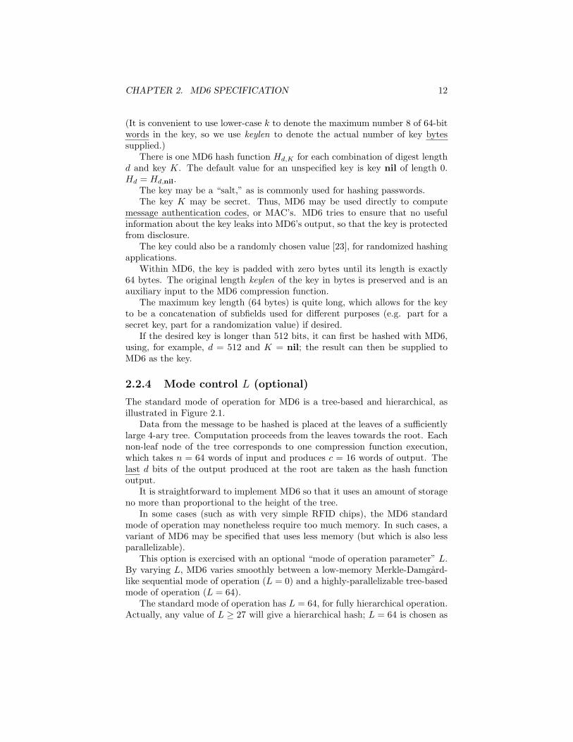
2.2.4 Mode control L (optional)
The standard mode of operation for MD6 is a tree-based and hierarchical, asillustrated in Figure 2.1.
Data from the message to be hashed is placed at the leaves of a sufficientlylarge 4-ary tree. Computation proceeds from the leaves towards the root. Eachnon-leaf node of the tree corresponds to one compression function execution,which takes n = 64 words of input and produces c = 16 words of output. Thelast d bits of the output produced at the root are taken as the hash functionoutput.
It is straightforward to implement MD6 so that it uses an amount of storageno more than proportional to the height of the tree.
In some cases (such as with very simple RFID chips), the MD6 standardmode of operation may nonetheless require too much memory. In such cases, avariant of MD6 may be specified that uses less memory (but which is also lessparallelizable).
This option is exercised with an optional “mode of operation parameter” L.By varying L, MD6 varies smoothly between a low-memory Merkle-Damgard-like sequential mode of operation (L = 0) and a highly-parallelizable tree-basedmode of operation (L = 64).
The standard mode of operation has L = 64, for fully hierarchical operation.Actually, any value of L ≥ 27 will give a hierarchical hash; L = 64 is chosen as
CHAPTER 2. MD6 SPECIFICATION 13
the default in order to represent a value “sufficiently large” that the sequentialmode of operation is never invoked.
Section 2.4 gives more details on MD6’s mode of operation.
2.2.5 Number of rounds r (optional)
The MD6 compression function f has a controllable number r of rounds. Roughlyspeaking, each round corresponds to one clock cycle in a typical hardware im-plementation, or 16 steps in a software implementation.
The default value of r is
r = 40 + bd/4c ; (2.1)
so Hd,K,L = Hd,K,L,40+bd/4c. For d = 160, MD6 thus has a default of r = 80rounds; for d = 512, MD6 has a default of r = 168 rounds. One may increaser for increased security, or decrease r for improved performance, trading offsecurity for performance.
However, we also require that when MD6 is used in keyed mode, that r ≥ 80.This provides protection for the key, even when the desired output is short (as itmight be for a MAC). Thus, when MD6 has a nonempty key, the default valueof r is
r = max(80, 40 + bd/4c) . (2.2)
The round parameter r is exposed in the MD6 API, so it may be explicitlyvaried by the user. This is done since reduced-round versions of MD6 may beof interest for security analysis, or for applications with tight timing constraintsand reduced security requirements. Or, one could increase r above the defaultto accommodate various levels of paranoia. Also, if there is a key, but it isnon-secret, then fewer than 80 rounds could be specified if desired.
Arguably, the current need to consider a new hash function standard mighthave seemed unnecessary if the API for the prior standards had included avariable number of rounds.
2.2.6 Other MD6 parameters
There are other parameters to the MD6 hash function that could also be varied,at least in principle (e.g. w, Q, c, t0 . . . t5, ri, `i, Si for 0 ≤ i < rc). For thepurpose of defining what “MD6” means, these quantities should all be consideredfixed with default values as described herein. But variant MD6 hash functionsthat use other settings for these parameters could be considered and studied.See Chapter 9 for a description of how these parameters might be varied.
2.2.7 Naming versions of MD6
We suggest the following approach for naming various versions of MD6.In the simplest case, we only need to specify the digest size: MD6-d specifies
the version of MD6 having digest size d. This version also has the zero-length
CHAPTER 2. MD6 SPECIFICATION 14
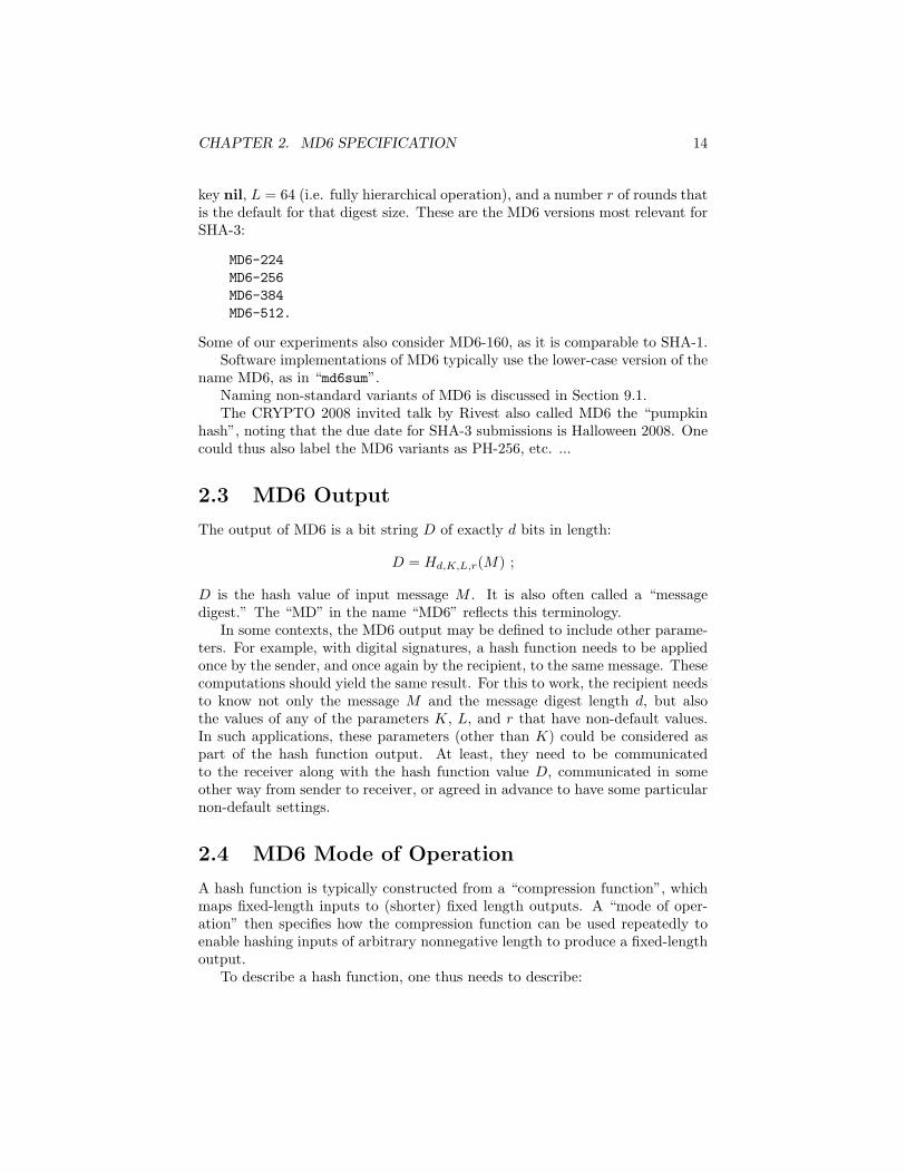
key nil, L = 64 (i.e. fully hierarchical operation), and a number r of rounds thatis the default for that digest size. These are the MD6 versions most relevant forSHA-3:
MD6-224MD6-256MD6-384MD6-512.
Some of our experiments also consider MD6-160, as it is comparable to SHA-1.Software implementations of MD6 typically use the lower-case version of the
name MD6, as in “md6sum”.Naming non-standard variants of MD6 is discussed in Section 9.1.The CRYPTO 2008 invited talk by Rivest also called MD6 the “pumpkin
hash”, noting that the due date for SHA-3 submissions is Halloween 2008. Onecould thus also label the MD6 variants as PH-256, etc. ...
2.3 MD6 Output
The output of MD6 is a bit string D of exactly d bits in length:
D = Hd,K,L,r(M) ;
D is the hash value of input message M . It is also often called a “messagedigest.” The “MD” in the name “MD6” reflects this terminology.
In some contexts, the MD6 output may be defined to include other parame-ters. For example, with digital signatures, a hash function needs to be appliedonce by the sender, and once again by the recipient, to the same message. Thesecomputations should yield the same result. For this to work, the recipient needsto know not only the message M and the message digest length d, but alsothe values of any of the parameters K, L, and r that have non-default values.In such applications, these parameters (other than K) could be considered aspart of the hash function output. At least, they need to be communicatedto the receiver along with the hash function value D, communicated in someother way from sender to receiver, or agreed in advance to have some particularnon-default settings.
2.4 MD6 Mode of Operation
A hash function is typically constructed from a “compression function”, whichmaps fixed-length inputs to (shorter) fixed length outputs. A “mode of oper-ation” then specifies how the compression function can be used repeatedly toenable hashing inputs of arbitrary nonnegative length to produce a fixed-lengthoutput.
To describe a hash function, one thus needs to describe:
CHAPTER 2. MD6 SPECIFICATION 15
• its mode of operation,
• its compression function, and
• various constants used in the computation.
The MD6 compression function f takes inputs of a fixed length (n = 89words), and produces outputs of a fixed but shorter length (c = 16 words):
f : W89 −→W16 .
(Recall that W is the set of all binary words of length w = 64 bits.)For convenience, we call a c-word block a “chunk”. The chaining variables
produced by MD6 are all “chunks”.The 89-word input to the compression function f contains a 15-word constant
Q, an 8-word key K, a “unique ID” word U , a “control word V ”, and a 64-worddata block B.
Since Q is constant, the “effective” or “reduced” MD6 compression functionfQ maps 74-word inputs to 16-word outputs:
fQ : W74 −→W16.
via the relationship:fQ(x) = f(Q||x) .
Thus, the MD6 compression function achieves a fourfold reduction in sizefrom data block to output—four chunks fit exactly into one data block, and onechunk is output.
The next section describes the MD6 mode of operation; Section 2.5 thendescribes the MD6 compression function.
2.4.1 A hierarchical mode of operation
The standard mode of operation for MD6 is tree-based. See Figure 2.1. Animplementation of this hierarchical mode requires storage at least proportionalto the height of the tree.
Since some very small devices may not have sufficient storage available, MD6provides a height-limiting parameter L. When the height reaches L + 1, MD6switches from the parallel compression operator PAR to the sequential com-pression operator SEQ.
The MD6 mode of operation is thus optionally parameterized by the integerL, 0 ≤ L ≤ 64, which allows a smooth transition from the default tree-basedhierarchical mode of operation (for large L) down to an iterative mode of oper-ation (for L = 0). When L = 0, MD6 works in a manner similar to that of thewell-known Merkle-Damgard method [65, 64, 34] construction or to the HAIFAmethod [18]. See Figure 2.2.
In our description of the MD6 mode of operation, MD6 makes up to L“parallel” passes over the data, each one reducing the size of the data by a
CHAPTER 2. MD6 SPECIFICATION 16
factor of four, and then performs (if necessary) a single sequential pass to finishup.
Since the input size must be less than 264 bits and the final compressionfunction produces an output of 210 = 1024 bits (before final truncation to dbits), there will be at most 27 such parallel passes (since 27 = log4(264/210).The default value L = 64, since it is greater than 27, ensures that by defaultMD6 will be full hierarchical.
Graphically, MD6 creates a sequence of 4-ary trees of height at most L, eachcontaining 4L leaf chunks (of c = 16 words each), then combines the valuesproduced at their roots (if there is more than one) in a sequential Merkle-Damgard-like manner.
If 4L is larger than the number of 16-word chunks in the input message, thenonly one tree is created, and MD6 becomes a purely tree-based method.
On the other hand, if L = 0, then no trees are created, and the input isdivided into 48-word (three-chunk) data-blocks to be combined in a sequentialMerkle-Damgard-like manner. (There are now only three data chunks in a datablock, since one chunk is the chaining variable from the previous compressionoperation at the node immediately to the left.)
For intermediate values of L, we trade off tree height (and thus minimummemory requirements) for opportunities for parallelism (and thus perhaps greaterspeed).
Figure 2.4 gives the top-level procedure for the MD6 mode of operation,which is described in a bottom-up, level by level manner.
First, all of the compression operations on level ` = 1 are performed. Thenall of the compression operations on level ` = 2 are performed, etc.
MD6 is described in this manner for maximum clarity. A practical imple-mentation may be organized somewhat differently (but, of course, in a way thatcomputes the same function). For example, operations at different levels may beintermixed, with a compression operation being performed as soon as its inputsare available. See Chapter 4 for some discussion of implementation issues.
Each such compression operation is by default performed with the PARoperation, described in Figure 2.5. The PAR operation may be implemented inparallel (hence its name). Given the data on level `−1, it produces the data onlevel `, which will be only one-fourth as large. This is repeated until a level isreached where the remaining data is only 16 words long. This data is truncatedto become the final hash output.
Figure 2.6 describes SEQ—it is very similar to Merkle-Damgard in opera-tion. It works sequentially through the input data on the last level and producesthe final hash output.
2.4.2 Compression function input
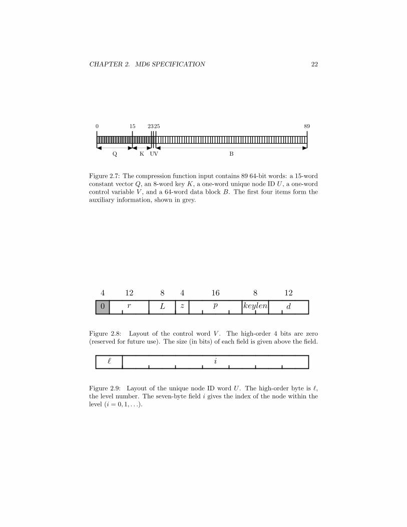
MD6’s mode of operation formats the input to the compression function f in thefollowing way. There are n = 89 words, formatted as follows with the defaultsizes. See Figure 2.7. The first four items Q, K, U , V , are “auxiliary inputs”,while the last item B is the data payload.
CHAPTER 2. MD6 SPECIFICATION 17
0
1
2
3
level
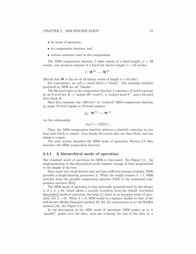
Figure 2.1: Structure of the standard MD6 mode of operation (L = 64). Com-putation proceeds from bottom to top: the input is on level 0, and the finalhash value is output from the root of the tree. Each edge between two nodesrepresents a 16 word (128 byte or 1024-bit) chunk. Each small black dot onlevel 0 corresponds to a 16-word chunk of input message. The grey dot on level0 corresponds to a last partial chunk (less than 16 words) that is padded withzeros until it is 16 words long. A white dot (on any level) corresponds to apadding chunk of all zeros. Each medium or large black dot above level zerocorresponds to an application of the compression function. The large black dotrepresents the final compression operation; here it is at the root. The final MD6hash value is obtained by truncating the value computed there.
0
1
level
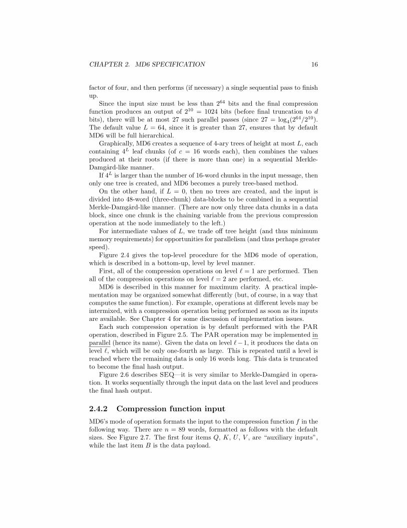
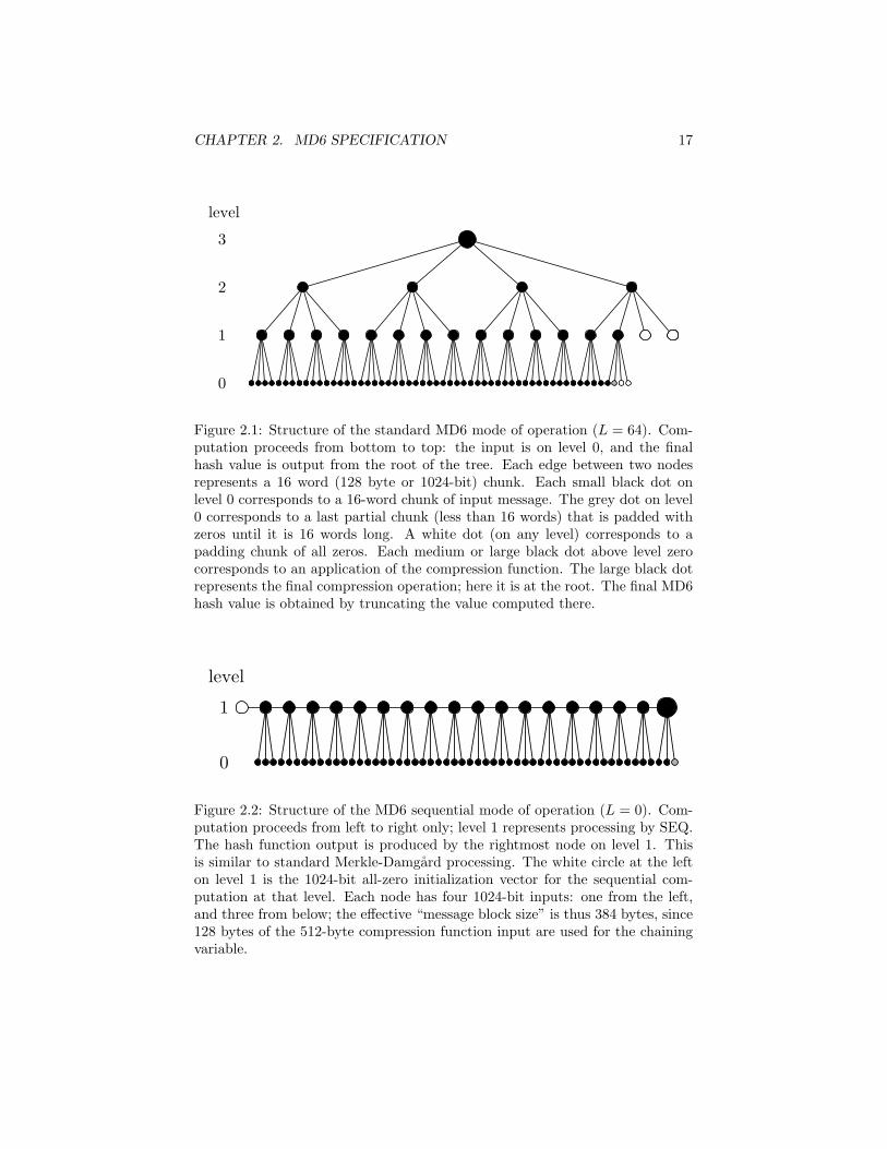
Figure 2.2: Structure of the MD6 sequential mode of operation (L = 0). Com-putation proceeds from left to right only; level 1 represents processing by SEQ.The hash function output is produced by the rightmost node on level 1. Thisis similar to standard Merkle-Damgard processing. The white circle at the lefton level 1 is the 1024-bit all-zero initialization vector for the sequential com-putation at that level. Each node has four 1024-bit inputs: one from the left,and three from below; the effective “message block size” is thus 384 bytes, since128 bytes of the 512-byte compression function input are used for the chainingvariable.
CHAPTER 2. MD6 SPECIFICATION 18
0
1
2
level
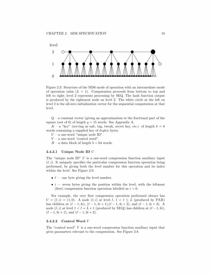
Figure 2.3: Structure of the MD6 mode of operation with an intermediate modeof operation value (L = 1). Computation proceeds from bottom to top andleft to right; level 2 represents processing by SEQ. The hash function outputis produced by the rightmost node on level 2. The white circle at the left onlevel 2 is the all-zero initialization vector for the sequential computation at thatlevel.
Q – a constant vector (giving an approximation to the fractional part of thesquare root of 6) of length q = 15 words. See Appendix A.
K – a “key” (serving as salt, tag, tweak, secret key, etc.) of length k = 8words containing a supplied key of keylen bytes.
U – a one-word “unique node ID”.V – a one-word “control word”.B – a data block of length b = 64 words.
2.4.2.1 Unique Node ID U
The “unique node ID” U is a one-word compression function auxiliary input(`, i). It uniquely specifies the particular compression function operation beingperformed, by giving both the level number for this operation and its indexwithin the level. See Figure 2.9.
• ` — one byte giving the level number.
• i — seven bytes giving the position within the level, with the leftmost(first) compression function operation labelled as i = 0.
For example, the very first compression operation performed always hasU = (`, i) = (1, 0). A node (`, i) at level `, 1 < ` ≤ L (produced by PAR)has children at (` − 1, 4i), (` − 1, 4i + 1),(` − 1, 4i + 2), and (` − 1, 4i + 3). Anode (`, i) at level 1 < ` = L+ 1 (produced by SEQ) has children at (`− 1, 3i),(`− 1, 3i+ 1), and (`− 1, 3i+ 2).
2.4.2.2 Control Word V
The “control word” V is a one-word compression function auxiliary input thatgives parameters relevant to the computation. See Figure 2.8.
CHAPTER 2. MD6 SPECIFICATION 19
The MD6 Mode of OperationInput:
M : A message M of some non-negative length m in bits.
d: The length d (in bits) of the desired hash output, 1 ≤ d ≤ 512.
K: An arbitrary k = 8 word “key” value, containing a supplied key of keylenbytes padded on the right with (64− keylen) zero bytes.
L : A non-negative mode parameter (maximum level number, or number ofparallel passes).
r : A non-negative number of rounds.
Output:
D: A d-bit hash value D = Hd,K,L,r(M).
Procedure:
Initialize:
• Let ` = 0, M0 = M , and m0 = m.
Main level-by-level loop:
• Let ` = `+ 1.• If ` = L+1, return SEQ(M`−1, d,K,L, r) as the hash function output.• Let M` = PAR(M`−1, d,K,L, r, `). Let m` denote the length of M` in
bits.• If m` = cw (i.e. if M` is c words long), return the last d bits of M`
as the hash function output. Otherwise, return to the top of the mainlevel-by-level loop.
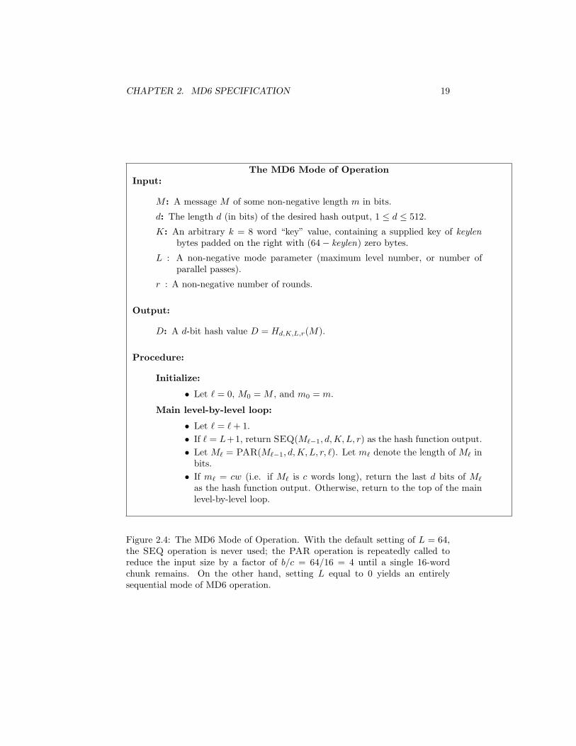
Figure 2.4: The MD6 Mode of Operation. With the default setting of L = 64,the SEQ operation is never used; the PAR operation is repeatedly called toreduce the input size by a factor of b/c = 64/16 = 4 until a single 16-wordchunk remains. On the other hand, setting L equal to 0 yields an entirelysequential mode of MD6 operation.
CHAPTER 2. MD6 SPECIFICATION 20
The MD6 PAR OperationInput:
M`−1: A message of some non-negative length m`−1 in bits.
d: The length d (in bits) of the desired hash output, 1 ≤ d ≤ 512.
K: An arbitrary k = 8 word “key” value, containing a supplied key of keylenbytes.
L : A non-negative mode parameter (maximum level number, or number ofparallel passes).
r : A non-negative number of rounds.
` : A non-negative integer level number, 1 ≤ ` ≤ L.
Output:
M`: A message of length m` bits, where m` = 1024 ·max(1, dm`−1/4096e)
Procedure:
Initialize:
• Let Q denote the array of length q = 15 words giving the fractionalpart of
√6. (See Appendix A.)
• Let f denote the MD6 compression function mapping 89 words of input(including a 64-word data block B) to a 16-word output chunk C usingr rounds of computation.
Shrink:
• Extend input M`−1 if necessary (and only if necessary) by appendingzero bits until its length becomes a positive integral multiple of b = 64words. Then M`−1 can be viewed as a sequence B0, B1, . . . , Bj−1 ofb-word blocks, where j = max(1, dm`−1/bwe).
• For each b-word block Bi, i = 0, 1, . . . , j − 1, compute Ci in parallel asfollows:– Let p denote the number of padding bits in Bi; 0 ≤ p ≤ 4096. (p
can only be nonzero for i = j − 1.)– Let z = 1 if j = 1, otherwise let z = 0. (z = 1 only for the last
block to be compressed in the complete MD6 computation.)– Let V be the one-word value r||L||z||p||keylen||d (see Figure 2.8).– Let U = `∗256 +i be a “unique node ID”—a one-word value unique
to this compression function operation.– Let Ci = f(Q||K||U ||V ||Bi). (Ci has length c = 16 words).
• Return M` = C0||C1|| . . . ||Cj−1.
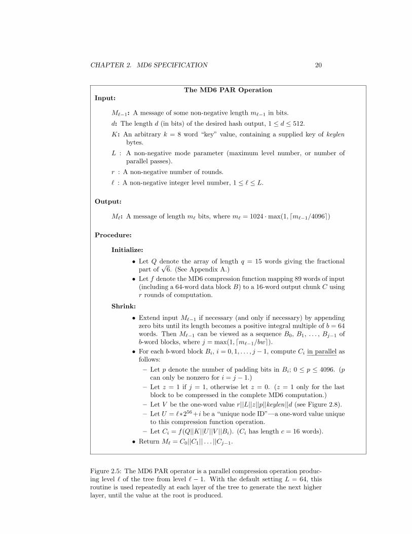
Figure 2.5: The MD6 PAR operator is a parallel compression operation produc-ing level ` of the tree from level ` − 1. With the default setting L = 64, thisroutine is used repeatedly at each layer of the tree to generate the next higherlayer, until the value at the root is produced.
CHAPTER 2. MD6 SPECIFICATION 21
The (Optional) MD6 SEQ OperationInput:
ML: A message of some non-negative length mL in bits.
d: The length d (in bits) of the desired hash output, 1 ≤ d ≤ 512.
K: An arbitrary k = 8 word key value, containing a supplied key of keylen bytes.
L : A non-negative mode parameter (maximum tree height).
r : A non-negative number of rounds.
Output:
D: A d-bit hash value.
Procedure:
Initialize:
• Let Q denote the array of length q = 15 words giving the fractionalpart of
√6. (See Appendix A.)
• Let f denote the MD6 compression function mapping an 89-word input(including a 64-word data block B) to a 16-word output block C usingr rounds of computation.
Main loop:
• Let C−1 be the zero vector of length c = 16 words. (This is the “IV”.)• Extend input ML if necessary (and only if necessary) by appending zero
bits until its length becomes a positive integral multiple of (b− c) = 48words. Then ML can be viewed as a sequence B0, B1, . . . , Bj−1 of(b− c)-word blocks, where j = max(1, dmL/(b− c)we).
• For each (b− c)-word block Bi, i = 0, 1, . . . , j− 1 in sequence, computeCi as follows:– Let p be the number of padding bits in Bi; 0 ≤ p ≤ 3072. (p can
only be nonzero when i = j − 1.)– Let z = 1 if i = j − 1, otherwise let z = 0. (z = 1 only for the last
block to be compressed in the complete MD6 computation.)– Let V be the one-word value r||L||z||p||keylen||d (see Figure 2.8).– Let U = (L+ 1) · 256 + i be a “unique node ID”—a one-word value
unique to this compression function operation.– Let Ci = f(Q||K||U ||V ||Ci−1||Bi). (Ci has length c = 16 words).
• Return the last d bits of Cj−1 as the hash function output.
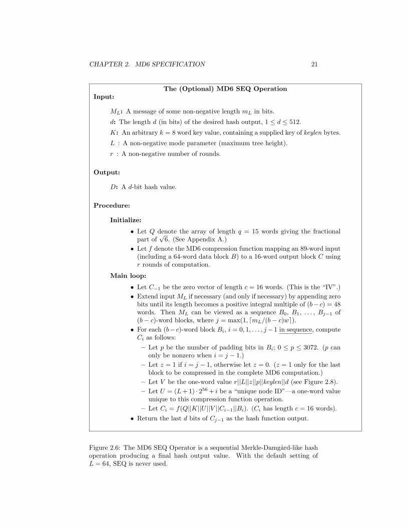
Figure 2.6: The MD6 SEQ Operator is a sequential Merkle-Damgard-like hashoperation producing a final hash output value. With the default setting ofL = 64, SEQ is never used.
CHAPTER 2. MD6 SPECIFICATION 22
Q K UV B
0 15 2325 89
Figure 2.7: The compression function input contains 89 64-bit words: a 15-wordconstant vector Q, an 8-word key K, a one-word unique node ID U , a one-wordcontrol variable V , and a 64-word data block B. The first four items form theauxiliary information, shown in grey.
0 r L z p keylen d
4 12 8 4 16 8 12
Figure 2.8: Layout of the control word V . The high-order 4 bits are zero(reserved for future use). The size (in bits) of each field is given above the field.
` i
Figure 2.9: Layout of the unique node ID word U . The high-order byte is `,the level number. The seven-byte field i gives the index of the node within thelevel (i = 0, 1, . . .).
CHAPTER 2. MD6 SPECIFICATION 23
• r — number of rounds in the compression function (12 bits).
• L — mode parameter (maximum level) (8 bits).
• z — set to 1 if this is the final compression operation, otherwise 0 (4 bits).
In Figures 2.1, 2.3, 2.2, these final operations are indicated by the verylarge black circles.
• p — the number of padding data bits (appended zero bits) in the currentinput block B (16 bits).
• keylen — the original length (in bytes) of the supplied key K (8 bits).
• d — the desired length in bits of the digest output (12 bits).
2.5 MD6 Compression Function
This section describes the operation of the MD6 compression function.The compression function f takes as input an array N of length n = 89
words. It outputs an array C of length c = 16 words.Here f is described as having a single 89-word input N , although it may
also be viewed as having a 25-word “auxiliary” input (Q||K||U ||V ) followed bya 64-word “data” input block B.
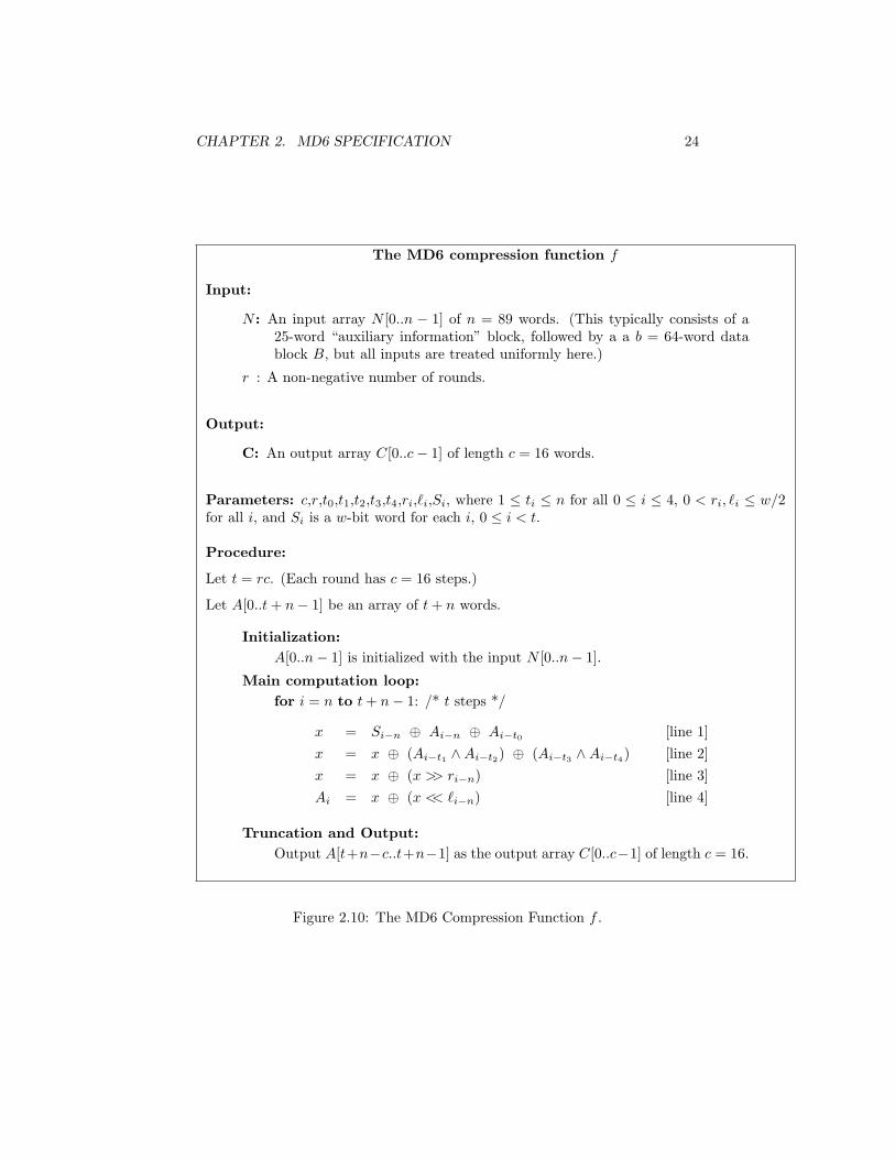
The compression function f is computed as shown in Figure 2.10.The compression function may be viewed as consisting of an encryption of
N with a fixed arbitrary key S (which is not secret), followed by a truncationoperation that returns only the last 16 words of ES(N). See Figure 2.11. HereS determines the “round constants” of the encryption algorithm.
Internally, the compression function has a main loop of r rounds (each con-sisting of c = 16 steps), followed by the truncation operation that truncates thefinal result to c = 16 words.
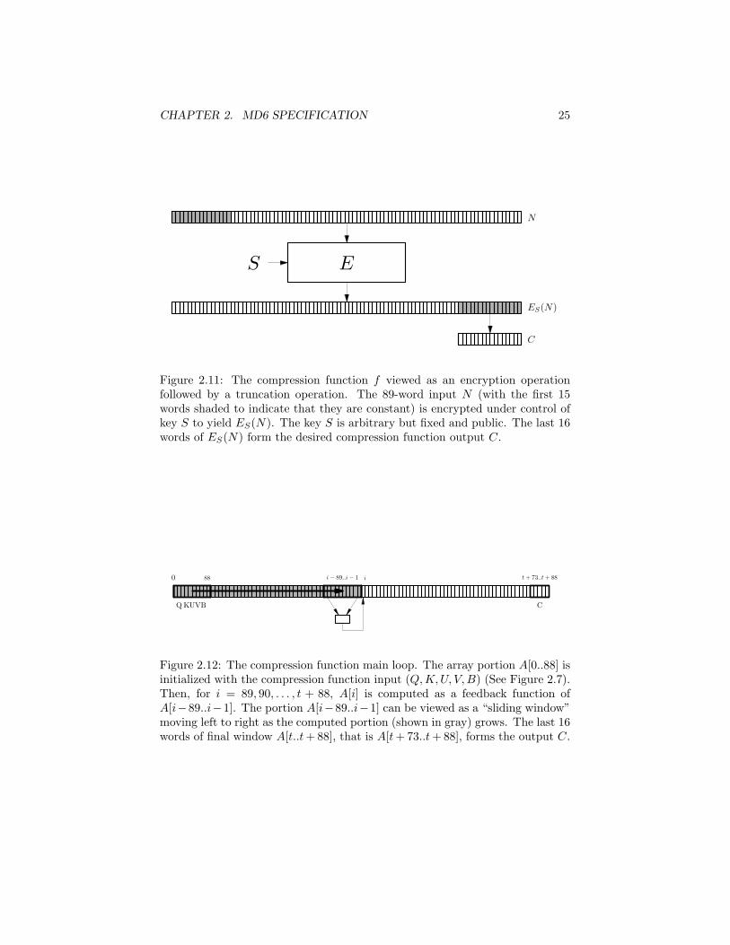
The main loop thus performs a total of t = rc steps, where each step com-putes a one-word value. This loop can be implemented by loading the inputinto the first n words of an array A of length n + t, then computing each ofthe remaining t words in turn. See Figure 2.12. Equivalently, this loop can beimplemented as a nonlinear feedback shift register with 89 words of state. SeeFigure 2.14.
The truncation operation merely returns the last 16 words of A as the com-pression function output (which we also call the “chaining variable”). Thecompression function always outputs c = 16 words (1024 bits) for this chain-ing variable. This is at least twice as large as any possible MD6 hash functionoutput, in line with the “wide-pipe” strategy suggested by Lucks [55].
The compression function takes the “feedback tap positions” t0, t1, t2, t3, t4,each in the range 1 to n−1 = 88, as parameters. (Note the slight overloading forthe symbol t: when subscripted, it refers to a tap position; when unsubscripted,it refers to the number of computation steps t = rc.)
CHAPTER 2. MD6 SPECIFICATION 24
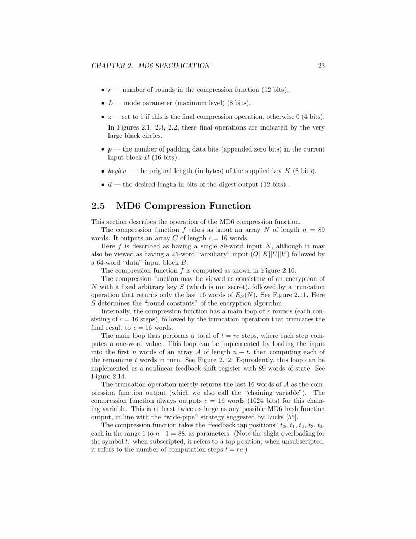
The MD6 compression function f
Input:
N : An input array N [0..n − 1] of n = 89 words. (This typically consists of a25-word “auxiliary information” block, followed by a a b = 64-word datablock B, but all inputs are treated uniformly here.)
r : A non-negative number of rounds.
Output:
C: An output array C[0..c− 1] of length c = 16 words.
Parameters: c,r,t0,t1,t2,t3,t4,ri,`i,Si, where 1 ≤ ti ≤ n for all 0 ≤ i ≤ 4, 0 < ri, `i ≤ w/2for all i, and Si is a w-bit word for each i, 0 ≤ i < t.
Procedure:
Let t = rc. (Each round has c = 16 steps.)
Let A[0..t+ n− 1] be an array of t+ n words.
Initialization:A[0..n− 1] is initialized with the input N [0..n− 1].
Main computation loop:for i = n to t+ n− 1: /* t steps */
x = Si−n ⊕ Ai−n ⊕ Ai−t0 [line 1]x = x ⊕ (Ai−t1 ∧Ai−t2) ⊕ (Ai−t3 ∧Ai−t4) [line 2]x = x ⊕ (x >> ri−n) [line 3]Ai = x ⊕ (x << `i−n) [line 4]
Truncation and Output:Output A[t+n−c..t+n−1] as the output array C[0..c−1] of length c = 16.
Figure 2.10: The MD6 Compression Function f .
CHAPTER 2. MD6 SPECIFICATION 25
N
ES(N)
C
S E
Figure 2.11: The compression function f viewed as an encryption operationfollowed by a truncation operation. The 89-word input N (with the first 15words shaded to indicate that they are constant) is encrypted under control ofkey S to yield ES(N). The key S is arbitrary but fixed and public. The last 16words of ES(N) form the desired compression function output C.
BVUKQ
0 i− 89..i− 188 t+ 73..t+ 88i
C
Figure 2.12: The compression function main loop. The array portion A[0..88] isinitialized with the compression function input (Q,K,U, V,B) (See Figure 2.7).Then, for i = 89, 90, . . . , t + 88, A[i] is computed as a feedback function ofA[i−89..i−1]. The portion A[i−89..i−1] can be viewed as a “sliding window”moving left to right as the computed portion (shown in gray) grows. The last 16words of final window A[t..t+ 88], that is A[t+ 73..t+ 88], forms the output C.
CHAPTER 2. MD6 SPECIFICATION 26
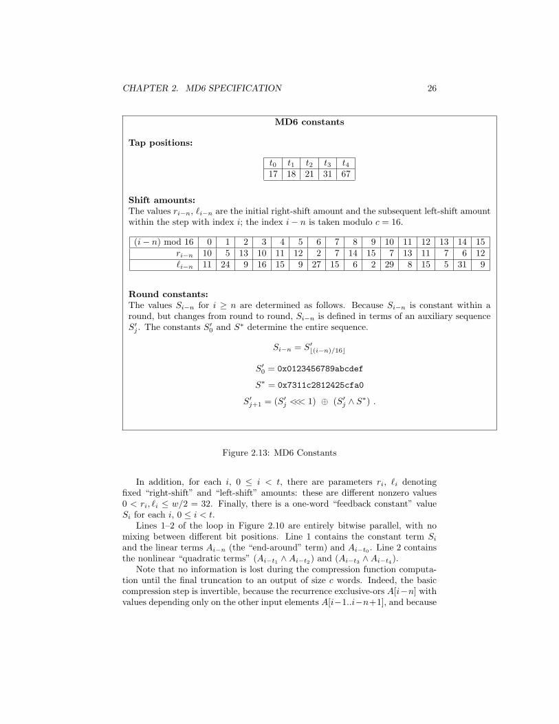
MD6 constants
Tap positions:
t0 t1 t2 t3 t417 18 21 31 67
Shift amounts:The values ri−n, `i−n are the initial right-shift amount and the subsequent left-shift amountwithin the step with index i; the index i− n is taken modulo c = 16.
(i− n) mod 16 0 1 2 3 4 5 6 7 8 9 10 11 12 13 14 15ri−n 10 5 13 10 11 12 2 7 14 15 7 13 11 7 6 12`i−n 11 24 9 16 15 9 27 15 6 2 29 8 15 5 31 9
Round constants:The values Si−n for i ≥ n are determined as follows. Because Si−n is constant within around, but changes from round to round, Si−n is defined in terms of an auxiliary sequenceS′j . The constants S′0 and S∗ determine the entire sequence.
Si−n = S′b(i−n)/16c
S′0 = 0x0123456789abcdef
S∗ = 0x7311c2812425cfa0
S′j+1 = (S′j <<< 1) ⊕ (S′j ∧ S∗) .
Figure 2.13: MD6 Constants
In addition, for each i, 0 ≤ i < t, there are parameters ri, `i denotingfixed “right-shift” and “left-shift” amounts: these are different nonzero values0 < ri, `i ≤ w/2 = 32. Finally, there is a one-word “feedback constant” valueSi for each i, 0 ≤ i < t.
Lines 1–2 of the loop in Figure 2.10 are entirely bitwise parallel, with nomixing between different bit positions. Line 1 contains the constant term Siand the linear terms Ai−n (the “end-around” term) and Ai−t0 . Line 2 containsthe nonlinear “quadratic terms” (Ai−t1 ∧Ai−t2) and (Ai−t3 ∧Ai−t4).
Note that no information is lost during the compression function computa-tion until the final truncation to an output of size c words. Indeed, the basiccompression step is invertible, because the recurrence exclusive-ors A[i−n] withvalues depending only on the other input elements A[i−1..i−n+1], and because
CHAPTER 2. MD6 SPECIFICATION 27
1t0t1t2t3t489
⊕⊕⊕
∧∧
⊕ gri,`iSi
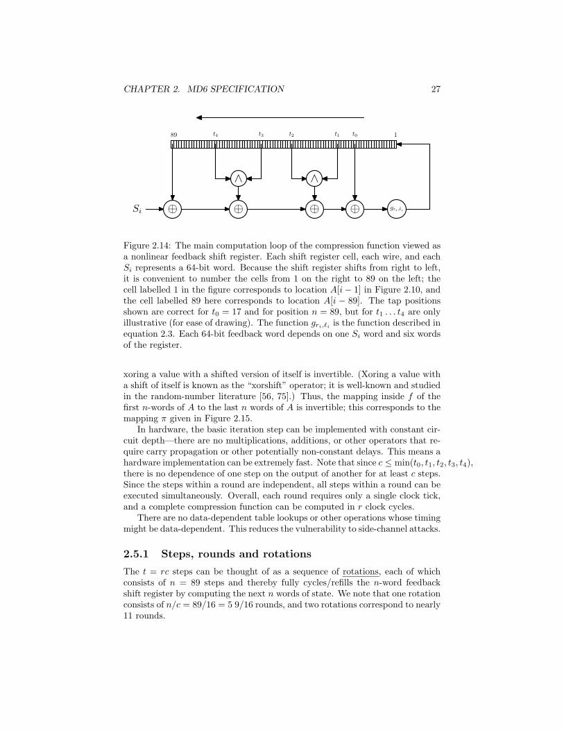
Figure 2.14: The main computation loop of the compression function viewed asa nonlinear feedback shift register. Each shift register cell, each wire, and eachSi represents a 64-bit word. Because the shift register shifts from right to left,it is convenient to number the cells from 1 on the right to 89 on the left; thecell labelled 1 in the figure corresponds to location A[i− 1] in Figure 2.10, andthe cell labelled 89 here corresponds to location A[i − 89]. The tap positionsshown are correct for t0 = 17 and for position n = 89, but for t1 . . . t4 are onlyillustrative (for ease of drawing). The function gri,`i is the function described inequation 2.3. Each 64-bit feedback word depends on one Si word and six wordsof the register.
xoring a value with a shifted version of itself is invertible. (Xoring a value witha shift of itself is known as the “xorshift” operator; it is well-known and studiedin the random-number literature [56, 75].) Thus, the mapping inside f of thefirst n-words of A to the last n words of A is invertible; this corresponds to themapping π given in Figure 2.15.
In hardware, the basic iteration step can be implemented with constant cir-cuit depth—there are no multiplications, additions, or other operators that re-quire carry propagation or other potentially non-constant delays. This means ahardware implementation can be extremely fast. Note that since c ≤ min(t0, t1, t2, t3, t4),there is no dependence of one step on the output of another for at least c steps.Since the steps within a round are independent, all steps within a round can beexecuted simultaneously. Overall, each round requires only a single clock tick,and a complete compression function can be computed in r clock cycles.
There are no data-dependent table lookups or other operations whose timingmight be data-dependent. This reduces the vulnerability to side-channel attacks.
2.5.1 Steps, rounds and rotations
The t = rc steps can be thought of as a sequence of rotations, each of whichconsists of n = 89 steps and thereby fully cycles/refills the n-word feedbackshift register by computing the next n words of state. We note that one rotationconsists of n/c = 89/16 = 5 9/16 rounds, and two rotations correspond to nearly11 rounds.
CHAPTER 2. MD6 SPECIFICATION 28
Each rotation produces a new n-word vector; you can view the computationas rc/n rotations, each of which produces a n-word state vector invertibly fromthe previous n-word state vector. The input is the first n-word state vector; theoutput is the last c words of the last n-word state vector. (Note that rc/n isn’tnecessarily an integer. That doesn’t matter here; the description just given isstill accurate.)
The compression function can also be viewed as r 16-step rounds each ofwhich computes the next 16 words of state.
We prefer the latter view.The MD6 feedback constants are organized in a manner that reflects the
round-oriented viewpoint. The round constant Si stays the same for all 16steps of a round and changes for the next round. The shift amounts r(·) and`(·) vary within a round, but then have the same pattern of variation withinsuccessive rounds.
For a software implementation of MD6, it is convenient to perform 16-foldloop-unrolling, so that each round is implemented as a branch-free basic blockof code.
2.5.2 Intra-word Diffusion via xorshifts
Some method is required to effect diffusion between the various bit positionswithin a word. This intra-word diffusion is provided by the gri,`i operatorimplicit in lines 3–4 of the loop in Figure 2.10:
gri,`i(x) = { y = x ⊕ (x >> ri);return y ⊕ (y << `i)}
(2.3)
(Here “`” and r are overloaded; `i and ri refer to a shift amounts, while rrefers to the number of rounds, and ` is used in the mode of operation to referto the level number; these distinctions should be clear from context.)
The function g is linear and invertible (lossless).The operators x = x ⊕ (x >> ri) and x = x ⊕ (x << `i) are known as
“xorshift” operators; their properties have been studied in [56, 75].
2.5.3 Shift amounts
The shift values are indexed mod c = 16 (i.e., they repeat every round).The values given here for MD6 were the result of extensive experiments using
one million randomly generated tables of such shift values. See Section 3.9.3
2.5.4 Round Constants
The round constants S′j provide some variability between round. Each roundj has its own constant S′j ; the steps within a round all use the same roundconstant.
CHAPTER 2. MD6 SPECIFICATION 29
The following recurrence generates these constants:
S′0 = 0x0123456789abcdef
S∗ = = 0x7311c2812425cfa0
S′j+1 = (S′j <<< 1) ⊕(S′j ∧ S∗) . (2.4)
This recurrence relation is one-to-one—from S′j one can determine S′j+1, andvice versa. (See Schnorr et al. [89, Lemma 5])
2.5.5 Alternative representations of the compression func-tion
There is another useful way of representing the compression function. Since the15-word portion Q of the input is a fixed constant, we can define the functionfQ as
fQ(x) = f(Q||x) ,
where fQ maps inputs of length n − q = 74 words to outputs of length c = 16words. This representation of f is useful in our security proofs of the compres-sion function in Section 6.1.2. We may refer to either f or fQ as “the MD6compression function”; they are intimately related. It is easier to talk aboutf when discussing the specification of MD6, but better to talk about fQ whendiscussing its security. We may refer to f as the “full” compression function,and fQ as the “reduced” compresssion function.
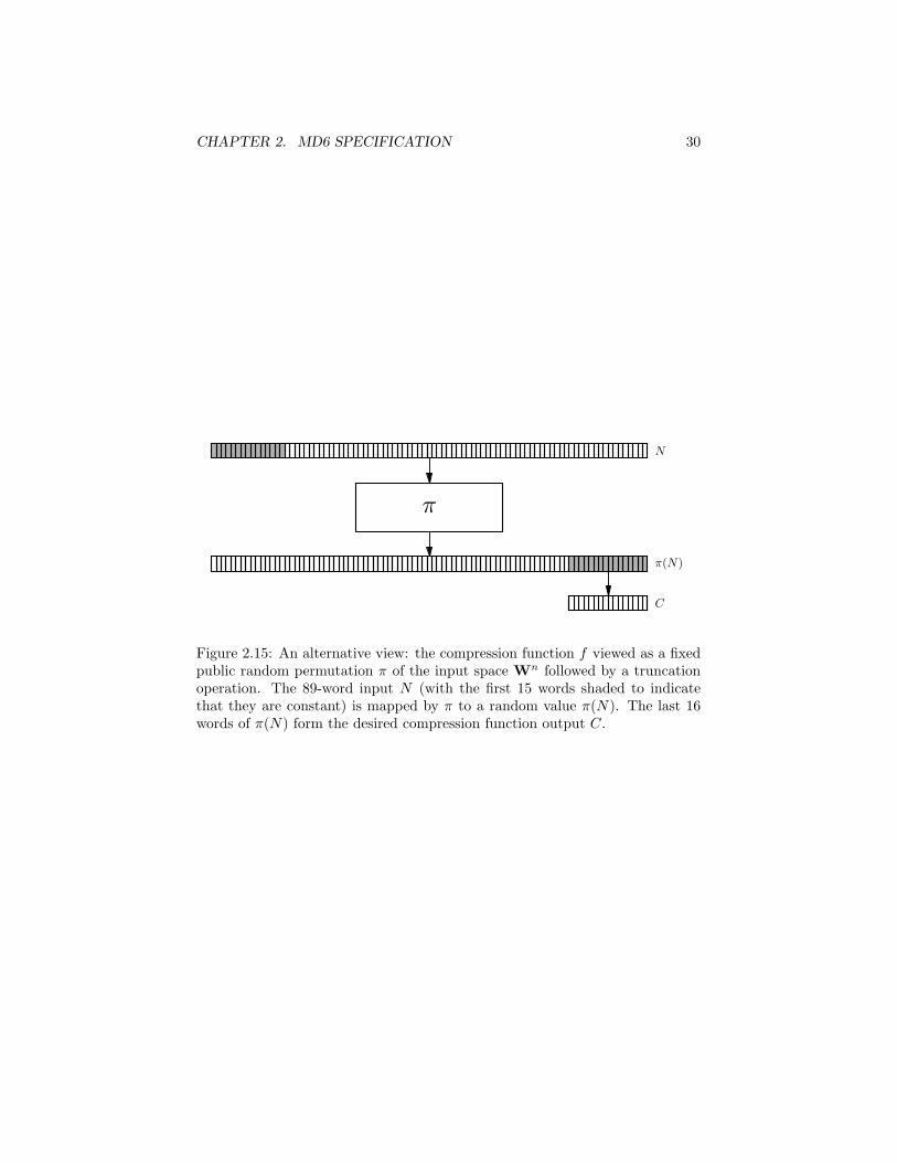
Another relevant representation is defined as follows. If we return to therepresentation of Figure 2.11, wherein f is defined in terms of an encryptionoperation, we note that S (and thus ES(·)) is public and fixed. It may thusbe preferable to view the compression function as a fixed but randomly cho-sen public permutation π of the input space Wn, followed by truncation to cwords. See Figure 2.15. We make use of this representation in our discussion ofcompression function security.
2.6 Summary
This chapter has presented the full specification of the MD6 hash function.Reference code provided with our submission to NIST for the SHA-3 competitionprovides a different, but equivalent, definition.
CHAPTER 2. MD6 SPECIFICATION 30
N
π(N)
C
π
Figure 2.15: An alternative view: the compression function f viewed as a fixedpublic random permutation π of the input space Wn followed by a truncationoperation. The 89-word input N (with the first 15 words shaded to indicatethat they are constant) is mapped by π to a random value π(N). The last 16words of π(N) form the desired compression function output C.
Chapter 3
Design Rationale
This chapter describes the considerations and reasoning behind many of thedesign decisions in MD6.
The landscape for designing hash functions has certainly changed in the lasttwo decades (since MD5 was designed)! Advances in technology have providedfewer constraints, and more opportunities. Theoretical advances provide newertools for the both the attacker and the designer.
The sections in this chapter summarize some of the considerations that wentin to the design choices for MD6. A related presentation of these issues isavailable in Rivest’s CRYPTO’08 slides (included with this submission).
Of course, the primary objective of a cryptographic hash function is security—meeting the stated cryptographic objectives. And, to the extent possible, doingso in a provable way. Chapters 6 and 7 provide detailed proofs regarding thesecurity properties of the MD6 compression function and mode of operation.
Some of the other significant considerations include:
• Increased availability of memory, allowing larger block sizes that includenew auxiliary inputs to each compression function call.
• The forthcoming flood of multicore CPU’s, some of which may containhundreds of cores. This consideration demands an approach that canexploit available parallelism.
• Side-channel attacks that limit the instructions that one deems “safe” inan application potentially utilizing secret keys.
The following sections document these and related considerations.
3.1 Compression function inputs
It is worthwhile to begin by revisiting the description of the inputs to a com-pression function and associated terminology.
31
CHAPTER 3. DESIGN RATIONALE 32
3.1.1 Main inputs: message and chaining variable
Traditionally, compression functions have two main input ports: one for achaining variable and one for a message block.
Such a traditional compression function can be characterized as a mappingfrom a c-word input chaining variable and a b-word input message block to ac-word output chaining variable:
f : Wc ×Wb →Wc (3.1)
Here W denotes the set of w-bit words. The compression function produces asingle chaining variable of length c words as the output.
Such traditional compression functions are “hard-wired” to fit within a cer-tain mode of operation. More precisely, these input ports are dedicated to theirparticular use within the Merkle-Damgard mode of operation.
The compression function signature (3.1) may also relate to the mannerin which the compression function is constructed. For example, the chainingvariable may be used as input to an encryption algorithm, as in the Davies-Meyer construction [63, Ch. 9].
To move beyond the Merkle-Damgard paradigm, we need to take a some-what more general and flexible view of compression, along the lines of a generalpseudo-random function with fixed input and output sizes.
Note, for example, in a tree-based hash algorithm like MD6, compressionfunctions working on the leaves of the tree have only message data as input, whilecompression functions higher in the tree contain no message data, but insteadconsists of several chaining variables passed up from their children nodes. It thusdoesn’t make sense to have a compression function with dedicated “message”and “chaining variable” inputs.
We thus consider for the moment revising our compression function signatureby dropping the specific c-word “chaining variable input”, and considering thecompression function to be a mapping from b words of main input to c wordsof output:
fB : Wb →Wc . (3.2)
(The subscript B here indicates that we are only considering the inputs corre-sponding to the B portion–the data payload.) We’ll see in a moment that we’llrevise this signature again, slightly.
Whether the bw input bits come from the message, or are chaining variablesfrom previous compression function operations, will depend on the details of themode of operation. We still call the output of a compression function compu-tation a “chaining variable,” even though the computations may be linked in atree-like or other manner, rather than as a chain as in Merkle-Damgard.
The compression ratio of a compression function is the ratio b/c of the num-ber of main input bits to the number of output bits. Ratios in the range 3–5are typical; MD6 has a compression ratio of 4. For MD6 the b = 4c main inputwords may consist of either message data (as for a leaf node) or four chainingvariables (from child nodes) of size c words each.
CHAPTER 3. DESIGN RATIONALE 33
3.1.2 Auxiliary inputs: key, unique nodeID, control word
A compression function may have “auxiliary” inputs in addition to the “main”inputs described above.
A traditional compression function doesn’t have any such auxiliary inputs,but recently there have been a number of proposals (such as [18, 85]) to includesuch inputs. Such auxiliary inputs can have great value in defeating or reducingvulnerabilities associated with the standard Merkle-Damgard mode of operation.They also facilitate proofs of security, as one can often treat restrictions of thecompression function to different auxiliary inputs as, essentially, independent-drawn random functions.
MD6 makes liberal use of such auxiliary inputs, which for MD6 are:
• a k-word “key” K,
• a u-word “unique node ID” U , and
• a v-word “control word” V .
If the total length of such auxiliary inputs is α = k + u + v words, then thecompression function has the signature:
fQ : Wα ×Wb →Wc . (3.3)
(The subscript Q here indicates that we are considering all inputs except theconstant value Q; the actual implementation of the MD6 compression functionalso incorporates a fixed constant “input” value Q, but we do not need to discussQ further here, as it is constant.)
3.2 Provable security
To the extent possible while maintaining good efficiency, MD6 is based onprovable security.
We provide numerous reductions demonstrating that the MD6 mode of op-eration achieves various security goals, assuming that the MD6 compressionfunction satisfies certain properties.
We also provide strong evidence that the MD6 compression function has thedesired properties. This includes not only statistical analysis and SAT-solverattacks, but also provable lower bounds on the workload required by certaindifferential attacks.
The tree-based MD6 mode of operation is also interesting in that certainof its proofs admit a tighter security reduction than the corresponding knownresults for the Merkle-Damgard mode of operation.
Our results on the mode of operation security relate to pre-image resistance,collision-resistance, pseudorandomness, and indifferentiability from a randomoracle.
CHAPTER 3. DESIGN RATIONALE 34
3.3 Memory usage is less of a constraint
Continuing improvements in integrated circuit and memory technology havemade memory usage much less of a concern in hash function design. While stilla concern for low-end devices, the situation is overall much improved, and onecan reasonably propose hash functions with significantly larger memory usagethan for designs proposed in the 1990’s. Doing so can provide significant benefitsin flexibility and security.
Indeed, MD5 was designed in 1991; 17 years have since passed. Since then,the memory capacity of chips has increased at about 60% per year, so suchchips now have over 1000 times as much capacity. Similarly, the cost per bit ofmemory has decreased at rate of about 30% per year.
Even “embedded” processors may have substantial amounts of memory. Anembedded processor today is typically an ARM processor: a 32-bit processorwith many kilobytes of cache memory and access to potentially many megabytesof off-chip RAM. Even simple “smart card” chips have substantial memory. Forexample, a typical SIM card in a cell phone is a Java Card with 64KB of code,16KB of EEPROM and 1KB RAM [26].
RFID chips are the most resource-constrained environment to consider. Atthe moment, they are so severely constrained that doing serious cryptographyon an RFID chip is nearly impossible. But even this is evolving quickly; RFIDchips with 8KB memory (ROM, not RAM) are now available. Programming arespectable hash function onto an RFID chip may soon be a realistic proposition.
Thus, it is reasonable to consider hash function designs that use memorymore freely than the designs of the early 1990’s.
We will thus take as a design goal that MD6 should be implementable usingat most 1KB RAM.
An MD6 compression function calculation can easily be performed within1KB of RAM, and for L = 0 the entire MD6 hash function fits well within the1KB RAM limit. Larger systems can use more memory for increased parallelismand greater efficiency by using the default value L = 64.
3.3.1 Larger block size
A major benefit of the increased availability of memory is the ability to usecompression functions with larger inputs.
MD4 and MD5 have message+chaining sizes of 512 + 128 = 640 bits. SHA-1 has message+chaining sizes of 512 + 160 = 672 bits. The first members ofthe SHA-2 family (SHA-224, SHA-256) have message+chaining sizes of 512 +256 = 768 bits, while SHA-384 and SHA-512 have message+chaining sizes of1024 + 512 = 1536 bits.
Such input block sizes are arguably too small for what is needed for SHA-3, where we want a hash function producing 512-bit outputs. The compressionfunction function must produce at least 512 bits of output, and preferably more.With 1536-bit inputs, we can barely get a compression factor of three. Thereis little room left over for auxiliary inputs, and no possibility of following the
CHAPTER 3. DESIGN RATIONALE 35
“double-width pipe” strategy suggested by Lucks [55], wherein chaining vari-ables are twice as large as the final hash function output.
Thus, MD6 chooses an input data block size of 512 bytes (i.e. 64 words, or4096 bits), and a compression factor of four for its compression function. Thecompression function output size is 1024 bits—twice as large as any messagedigest required for SHA-3, so MD6 can follow the double-width pipe strategy.
Many benefits follow from having relatively large compression function in-puts.
First, having large inputs allows us to easily incorporate nontrivial auxiliaryinputs into the compression function computation, since these auxiliary inputsthen take up a smaller fraction of the compression function inputs.
Second, large inputs allows for more potential parallelism within the com-pression function computation. In MD6, all 16 steps within a single round canbe computed at once in parallel.
Third, a large message input block can accommodate a small message withina single block. For example, 512 bytes is a common size for disk blocks on ahard drive; such a block can be hashed with a single compression function call.Similarly, a network packet of up to 512 bytes can be hashed with a singlecompression function call.
Fourth, having a larger compression function input block should make crypt-analysis (even automated cryptanalysis) more difficult, since the number ofcompression function computation steps also increases. For example, with adifferential attack, the probability of success typically goes down exponentiallywith the number of computation steps. Existing hash functions have a numberof computation steps that may be fewer than the number of hash function out-put bits desired, whereas MD6 has many more than 512 steps. If each such stephas a probability of at most 1/2 of following a given differential path, then thelarge number of computation steps under MD6 makes such attacks very unlikelyto succeed.
3.3.2 Enabling parallelism
A second major benefit of the increased availability of memory is the ability toenable parallel computation.
SHA-3 should be able to exploit the paral-lelism provided by the forthcoming flood ofmulticore processors.
Yet, a parallel approach requires more memory than a sequential approach.In the best case, a tree-based approach requires memory at least proportionalto the height of the tree–that is, is, it requires memory at least proportional tothe logarithm of the message size. With a branching factor of 4, a leaf size of4096 bits, and a maximum message size of 264 bits, this logarithmic factor is 26.
CHAPTER 3. DESIGN RATIONALE 36
On a typical desktop computer, storage of 26 · 512 bytes (less than 14KB)is a trivial consideration. The easy availability of memory enables a multicoredesktop to hash large files and streams very quickly in parallel.
3.4 Parallelism
We are at a transition point in the design of processors.No longer can we expect clock rates to continue to increase dramatically with
each processor generation. Indeed, clock rates may have plateaued, after havingincreased by a factor of 4000 in the last ten years. The reason is that processorpower usage increases linearly with clock frequency, with all other things beingequal. (In practice, all other things aren’t equal, and the power usage increasesnonlinearly, perhaps even quadratically or cubically, with clock frequency.) Fur-ther increases in clock rate would require exotic cooling technologies to handlethe extremely high power densities that would result from the high clock rates.
Instead, performance gains will now be obtained mostly through the useof parallelism—specifically, through the use of multicore processors. Dual andquad-core processors are now easily available, and processors with more coresare becoming so. We can reasonably expect the number of cores per processorto double with each successive processor generation, while the clock rates maychange little, or even decline slightly.
Anwar Ghoulum, at Intel’s Microprocessor Technology Lab, says “developersshould start thinking about tens, hundreds, and thousands of cores now.”
A related expected trend is that, an increase in the parallel computationalpower of chips (measured as transistors × clock rate) compared to their I/Obandwidth, as transistor density improves faster than that of I/O pins and pads.Over the next 15 years, this ratio is expected to roughly quadruple, while serialcomputational power (measured in clock rate) compared to chip I/O bandwidthwill decrease by a factor of roughly 10.1 Hence, in the long term parallelizablefunctions can afford more computation (and, hopefully, higher security) for agiven level of I/O utilization.
A tree-based design is the most natural approach for exploiting parallelismin a hash function. Ralph Merkle’s PhD thesis [65] described the first suchapproach, now known as “Merkle trees.” The computation proceeds from theleaves towards the root, with each tree node corresponding to one compressionfunction computation. If the compression function has a compression factor of4, then each tree node will have four children. MD6 follows this approach.
Damgard [34] also described parallel approaches to hash functions. Thesemethods can be viewed as constructing a tree by a level-by-level bottom-upcomputation, wherein the nodes within each level of the tree are computed inparallel. Damgard also suggested stopping the parallel level-by-level compu-tation after some fixed number of levels, and finishing up what is left with asequential computation. MD6 also follows this approach when L is small; here
1These figures apply to high-performance chips and are derived from the InternationalTechnology Roadmap for Semiconductors 2007 [40], specifically Tables 1i/j, 3a/b and AP2a/b.
CHAPTER 3. DESIGN RATIONALE 37
L (which he calls j) describes the number of levels to compute in parallel beforeswitching to a sequential mode of computation.
Other authors have also explored parallel or tree-based hash function design.Perhaps most relevant to MD6 are various interesting and excellent proposalsby P. Sarkar, such as [88]. His constructions are somewhat different, however,in that message input values are consumed at every tree node, not just at theleaves.
MD6 thus adopts a tree-based approach for maximum parallelizability.However, there is definitely a trade-off between parallelizability and memory
usage; a fully parallelizable approach may have a memory footprint that is toolarge for some small embedded devices.
Therefore, MD6 follows Damgard’s lead by parameterizing the amount ofparallelization. MD6 allows the user to set the parameter L to be the numberof parallel passes before switching to a sequential mode. By setting L to 0, MD6acts in a purely sequential mode and uses minimal memory (under 1KB). Bysetting L large, parallelism is maximized and memory usage is proportional tothe logarithm of the input message size. (The value of L should of course becommunicated along with the hash function output in cases where MD6 is usedwith a non-standard value.)
3.4.1 Hierarchical mode of operation
The initial design for MD6 did not have a parameter L controlling the mode ofoperation; the hash was always fully hierarchical.
However, it was felt that (a) there might be substantial need for an MD6version that met tighter storage limits, and (b) it was easy to add an optionalcontrol parameter L that limits the height of trees used (and thus the storageused).
For small L, MD6 makes a collection trees of height at most L (which canbe done in parallel), and then, if there is enough data to make more than onesuch tree, combines their root values with a sequential Merkle-Damgard pass.
When L > 0, an implementation with infinite parallelism could compute allof the trees in time L, leaving a sequential computation requiring time O(m/4L),where m is the size of the original message.
In practice, infinite parallelism is unavailable, but even so, using MD6 tohash a long message on a multicore processor with P processors can result in aspeedup by a factor of P , for any P reasonable to imagine over the next severaldecades.
Envisioning that multi-core processors will be very common, we set thedefault value for an unspecified L to be L = 64 (giving tree-based hashing):Hd,K = Hd,K,64.
However, applications on very restricted processors may wish to choose L = 0for a purely sequential hash function with minimal memory requirements.
CHAPTER 3. DESIGN RATIONALE 38
3.4.2 Branching factor of four
A very early version of the MD6 design had chaining variables of size 512 bitsand a branching factor of eight (instead of the current branching factor of four).However, it was felt to be more important to ensure that the wide-pipe principlewas maintained for all values of d (particularly for d = 512, where securityrequirements are the toughest), so the chaining variable size was increased to1024 bits.
It would be possible, of course, to maintain the wide-pipe principle, whileimproving the branching factor when d < 512. For example, one could havec = 1024 for d = 512 or d = 384 (a branching factor of four), and c = 512 ford = 256 or d = 224 (a branching factor of eight). But this adds complexity anddoesn’t actually do much in terms of improved efficiency (it makes a differenceof about 16%), since almost all of the actual work is in the leaves.
3.5 A keyed hash function
Many existing hash functions, like MD5 and the SHA hash functions, are“keyless”—there is only one version of a hash function (per digest size). Thereis no standardized way to supply a key, salt, or index value to get differentversions of the hash function.
However, it is often proposed to convert a hash function into a MAC (messageauthentication code) by augmenting the hash function message input with asecret key input that is shared between sender and receiver.
The natural ways of doing this, however, turn out to be fraught with unex-pected risks [49, 82, 83]; the usual Merkle-Damgard iterative structure of a hashfunction interacts badly with the idea of just appending and/or prepending thesecret key to the message. With some care, however, it can be done; HMAC isone such approach [6] that is popular and well-studied.
There are other approaches, such as the “XOR-MAC” of Bellare et al. [7].For our purposes, XOR-MAC is interesting because (a) the key is involved inevery block of the computation and (b) the position i of the i-th block is involvedin the computation on the i-th block. (MD6 shares these properties.) However,the XOR-MAC construction doesn’t work at all for unkeyed hash functions orfor applications where the key is public, since the outer XOR’s can be defeatedby suitable use of linear algebra to produce inversions or collisions.
There are also other applications of keyed hash functions. For example, itis common to “salt” the computation of a hash function on a password beforestoring it. Here is salt is effectively a non-secret key (or index). The use of thesalt provides variability so that an adversary can’t easily pre-compute a dictio-nary of the hashes of commonly used passwords; he has to redo the computationfor each such salt.
See Bellare and Ristenpart [10] for further excellent discussion of keyed hashfunctions and their advantages.
In some situations, it is useful to choose keys randomly; this yield randomized
CHAPTER 3. DESIGN RATIONALE 39
hashing techniques [23], with many interesting applications and security bene-fits.
MD6 has a 64-byte (that is, 512-bit) “key” that may be used as a secretkey for a MAC, a public value for a salt, or as a randomized index for the hashfunction.
The reasons for making the key input relatively large are: (a) having a largeinput block size makes this relatively cheap, (b) it allows for easy use of text-based keys, and (c) it enables the use of MD6 outputs (even 512-bit outputs)as keys. The last advantage makes it possible to hash a very long value for useas a key in some other hash computation.
The MD6 key is actually of variable length (between 0 and 512 bits, inclu-sive). By preserving the original length of the supplied key in the control word,we ensure that the MD6 key doesn’t suffer from certain “extension” or “related-key” attacks—a key K and a key K ′ will cause MD6 to behave differently evenif K is a prefix of K ′.
3.6 Pervasive auxiliary inputs
As noted above, in MD6, auxiliary inputs are supplied to each compressionfunction computation. This point is worth emphasizing and elaborating.
3.6.1 Pervasive key
For example, the MD6 key is an auxiliary input to every compression functioncomputation. The key is not just, say, appended or prepended to the message.The pervasive presence of the key prevents length-extension attacks and othermischief.
3.6.2 Pervasive location information: “position-awareness”
Also, each compression function operation “knows where it is”—the unique nodeID U specifies exactly where the present compression function invocation lies inthe dataflow graph. We call this “position-awareness”.
Haifa [18] proposed such position-awareness for sequential Merkle-Damgard-like computations. MD6 generalizes this to tree-based hash functions—the com-pression function at a node has as input its level number and its position withinthe level. Moreover, it knows whether or not it is the “final” (or “root”) node.
Such position-awareness provides major benefits in addressing number ofvulnerabilities for non-position-aware modes of operation. The reason is thatany hash function subcomputation (i.e. a sub-chain or subtree) can only beused in one place in the overall computation.
In other words, position-awareness precludes “cut-and-paste” attacks—movinga hash-function computation from one place to another. They also preclude at-tacks (such as Kelsey’s) that perform hash function subcomputations, hopingthat they will fit in “somewhere” to produce a collision.
CHAPTER 3. DESIGN RATIONALE 40
3.6.3 Pervasive control word information
MD6 also has “control words” supplied pervasively to each compression functioncomputation.
The control words also specify the structure of the tree, by indicating howmany message bits are in each leaf node and how many children are present foreach non-leaf node. The MD6 control words specifies amount of “padding” ateach node and the node’s level number. This representation makes unnecessarythe use of traditional padding techniques (such as appending a one, then asmany zeros as necessary) while still uniquely specifying the tree structure.
Also, the root of the tree is specially marked via a bit in the control word.That is, the compression function computing the final output value is distin-guished; it has an input z = 1 that doesn’t occur for any other node. This hasbenefits for preventing various forms of “extension attacks” and other mischief.
Such pervasive structural information ensures that the length of the under-lying message (at the leaves the tree) is uniquely represented. (MD6 does notexplicitly represent the overall length of the message as an explicit input to anyone compression function computation; rather it is uniquely determined by thetree structure information represented as inputs to each node.)
The control words also specify other information about the desired compu-tation: the desired hash function output size d, the number r of rounds, theoptional “mode parameter” L, and the length of the key K.
The incorporation of the control word V helps to ensure that the hash func-tion indeed acts like a “new, unrelated” function whenever any of the compo-nents of the hash function change. Otherwise, for example, changing the outputhash size or the number of rounds might yield outputs that are clearly relatedto the original outputs.
In general, MD6 follows a policy of “pervasive explicitness.” As we havelearned through many painful lessons in cryptographic protocol design, leavingparameters implicit is a good recipe for introducing vulnerabilities. The same istrue in hash function design (e.g. the lack of position-awareness). It is better tomake sure that each potentially relevant or descriptive parameters is explicitlyan input to each compression function.
3.7 Restricted instruction set
MD6 is defined in terms of a very restricted set of logical operations, givingadvantages in terms of security, simplicity, and efficiency.
3.7.1 No operations with input-dependent timing
Timing attacks have turned out to be surprisingly effective against cryptosys-tems that utilize primitive operations whose running time depends upon theinput data being manipulated. We have thus learned to avoid whenever possi-ble:
CHAPTER 3. DESIGN RATIONALE 41
• Complex instructions such as multiplications and divisions whose runningtime may be faster when their inputs are simpler (as exploited, e.g., byBrumley et al. [22]).
• Shift or rotate instructions with input-dependent shift or rotate amounts.
• Input-dependent conditional branches (exploited, e.g, by Aciicmez et al. [1][2]).
• Table-lookup instructions where the table index is input-dependent. Dueto cache effects, such instructions can cause input-dependent running timefor both the cryptographic code itself (e.g., by Tsunoo et al., [93], Bern-stein [12] and Osvik et al. [74]) and independent adversarial processes onthe same processor (e.g., Osvik et al. [74][92] and Percival [76]).
The last limitation (no table-lookups) precludes the use of one of cryptog-rapher’s favorite components, the “S-box”, unless the the S-box is sufficientlysmall to be implemented purely in registers or via bitslicing.
3.7.2 Few operations
The MD6 compression function is implementable using only a very small set oflogical operations (on 64-bit words):
• XOR: the bit-wise exclusive-or of two words
• AND: the bit-wise and of two words
• FIXED SHIFT: the left-shift or right-shift of an input word by a fixedamount (with zeros shifted in).
Other operations can be built from these in the usual way:
• NOT: By XORing with 0xFF...FF, the all-ones word:
• OR: Using DeMorgan’s Law: (x ∨ y) = x ∧ y.
• FIXED ROTATE: Using two fixed shift operations, and OR.
3.7.3 Efficiency
All of the above instructions can be implemented in constant time regardless ofthe word size; there are no carry-propagations to worry about, for example, asthere would be for an adder.
(A 64-bit adder is rather useful for computing the “unique node ID” U inthe MD6 mode of operation. But here the nodeID is just a counter; there are nodata-dependent inputs. The addition counter increment can be performed usingthe above data-independent instructions (somewhat awkwardly), or by using aregular addition instruction or circuit. Since it is computed outside the innerloop, it was felt that the use of standard binary notation for the nodeID counterwas more helpful in terms of clarity of design than the “purity” of trying topurge all possible uses of addition from the design. Conversely, the recurrencefor S inside the inner loop was chosen to avoid the use of additions.)
CHAPTER 3. DESIGN RATIONALE 42
3.8 Wide-pipe strategy
The size of the intermediate chaining variables (linking one portion of the hashcomputation to another) may have a very significant effect on the security ofthe overall scheme.
Stefan Lucks was the first to articulate [54, 55] the important of the size ofthese internal variables, stating,
“The size of the internal hash values is a security parameter in itsown right.”
Lucks proposed the “wide-pipe” strategy, wherein the internal chaining vari-ables have a size that is independent of (and larger than) the final hash functionoutput. In the double-pipe strategy, the internal variables are twice as long asthe final hash function output.
A double-pipe strategy ensures that the chance that two chaining variablescollide (have the same value) is essentially negligible. The double- (or wide-)pipe strategy is an effective anti-dote that an adversary might otherwise ob-tain from the birthday paradox, as in recent “multicollision attacks” studied byJoux [46], Nandi et al. [68, 69] Hoch et al. [44], and Yu et al. [98].
A wide-pipe strategy has been invoked in other recent designs, such as [13].MD6 adopts a wide-pipe strategy: all internal chaining variables are cw =
1024 bits in length, which is at least twice the length of the final hash functionoutput.
3.9 Nonlinear feedback shift register
Many hash functions can be easily viewed as an NLFSR, with the understandingthat each step also makes use of additional inputs. For example, MD4 looks likea NLFSR with four 32-bit words of state.
MD6 places all inputs in the shift register before the computation begins,and has no non-constant inputs entering “from the side.”
Because there are no inputs “from the side”, it may be more difficult for acryptanalyst to find differential attacks on the collision-resistance of MD6.
The regular structure of the NLFSR also facilitates many aspects of oursecurity analysis.
The following subsections discuss some of the details of the design choicesmade in implementing the MD6 compression function as a NLFSR.
3.9.1 Tap positions
The tap positions t0, t1, and t2 are intentionally chosen to be somewhat small, sothat differences will propagate more rapidly. On the other hand, mini(ti) = 17is not too small, in order to support parallelism within the compression functioncomputation.
CHAPTER 3. DESIGN RATIONALE 43
Note that gcd(t0, n) = gcd(t1, n) = gcd(t2, n) = gcd(t2 − t1, n) = gcd(t4 −t3, n) = 1.
The tap positions t0,. . . ,t4 were chosen as follows:
• The tap position t0 = 17 was chosen to be relatively small (for fasteravalanche effect), yet not too small (so that MD6 can exploit parallelismby computing a full round in parallel), and relatively prime to the lengthof a round (so that different shift amounts come in to play during thefeedback propagation). This tap is a linear feedback position for fastestavalanche.
• The tap position n = 89 was necessarily chosen as a tap position for linearfeedback since we wish the feedback operation to be invertible (that is, wecan compute Ai−n from Ai−n+1..i; that is, we can run the shift register“backwards”).
• All tap positions were chosen to be nonzero modulo c = 16 and to havedifferent residues modulo c = 16. This minimizes possible negative inter-actions from basing shift amounts on the step size modulo 16. The tappositions must also satisfy t4 − t3 6= t2 − t1, so that the “and” gates willpair inputs at different distances from each other.
• Tap positions t1,. . . ,t4 were chosen using a computer search. It was de-termined by a simple brute force search that the chosen values (t1 = 18,t2 = 21, t3 = 31, and t4 = 67) minimize “dep” (here equal to 102), where“dep” has the property that if at least “dep” computation steps are per-formed, then each of the c most recent values computed is guaranteedto depend (in a formal sense) on all 89 input words to the compressionfunction. The program (tapopt.c) is available. See Table 9.1.
3.9.2 Round constants
As noted earlier, the recurrence relation 2.4 for the round constants is one-to-one(see Schnorr et al. [89, Lemma 5]).
Andrew Sutherland, who developed some great algorithms and tools fordetermining the orders of elements in groups for his Ph.D. thesis [91], determinedwith only a few seconds of computer time that the sequence S′j has period
6052837899185946603= 3 ∗ 3 ∗ 7 ∗ 59 ∗ 233 ∗ 1103 ∗ 2089 ∗ 3033169≈ 262.4 .
Of course, for MD6, we don’t need more than the first two hundred of theseelements, so the actual period length doesn’t matter as long as it isn’t veryshort.
CHAPTER 3. DESIGN RATIONALE 44
3.9.3 Intra-word diffusion operation g
We originally considered obtaining intra-word diffusion by using rotations ofwords, but a rotation is typically implemented using two shifts, and it seemslikely that two shifts can yield more benefit than simply using them to implementa rotation.
Note that whatever shifts are chosen (as long as ri 6= `i), a one-bit changeto the input of g will cause from two to four bits of the output of g to change.
Note also that g is one-to-one (i.e., invertible). An input change of any sortalways causes an output change.
To find shift values ri, `i, 0 ≤ i < c that provide a good diffusion operatorg, we ran a computer search. The shifts in g were determined by a computersearch. The program (shiftopt2.c) is available. It attempts to maximize therate of diffusion, given the tap positions and subject to some constraints on thechoice of r and ` values.
The following constraints were observed (they are heuristic in nature, andwere felt to improve the quality of the design, although a straightforward ran-domly generated table might do nearly as well). Each shift value must benonzero and at most w/2, and ri and `i must not be multiples of each other.The function gri,`i must be such that an output of hamming weight one can-not be generated by an input word of weight less than five. If w ≥ 32,then ri and `j must also not be multiples of each other, for any j such that(i− j) ∈ {t0, t5, t5− t0} (all subscripts taken modulo c). These latter conditions(which are hard to satisfy for w < 32) help ensure that a left shift in one roundis not followed by a right shift of the same amount (or a multiple thereof) in alatter round.
A table of shift values was chosen to provide the fastest avalanche effectamong those examined. The program for computing these shift tables is avail-able.
The operations x = x ⊕ (x << a) and x = x ⊕ (x >> b) are knownas xorshift operations in the random-number literature. They were recentlyintroduced by Marsaglia [56], and studied by Panneton and L’Ecuyer [75]. Ourusage is vaguely similar to Marsaglia’s proposal, although MD6 is considerablymore complex than Marsaglia’s simple generator. (As it should be, as MD6must meet cryptographic requirements that are not relevant for a simple randomnumber generator.)
3.9.4 Constant Vector Q
The presence of the constant vector Q helps to defeat inversion attacks, sincesomeone working the compression function backwards from a desired outputwould need to match all the bits in Q.
For the purposes of security analysis, Q should be considered as hard-wired;it is truly a constant. Although we talk about it as an “input” to the compressionfunction, it is a constant input that may not vary. Thus, for example, it doesn’tcount as “inverting” the compression function to come up with an input N =
CHAPTER 3. DESIGN RATIONALE 45
(Q,K,U, V,B) where Q has a value other than the standard fixed constantvalue. Our calling Q an “input” is merely for for expository convenience; thetrue inputs to the compression function are just B, V , U , and K. Producing“inputs” to the compression function with a different value of Q is no morelegitimate than “solving” an equation 7x5 − y2 = 1 by giving a solution for“a different value of 7”. In our security analysis, therefore, we focus on thecompression function fQ mapping Wn−q to Wc induced by fixing the Q inputto f .
3.10 Input symmetry
The MD6 compression function doesn’t treat any of its inputs (B,V ,U ,K, orQ) in any special manner; they are treated essentially “uniformly”. This can beformalized in the following design principle:
Principle of Input Symmetry: For any fixed permutation π ofthe nw input bit positions to the MD6 compression function, thesecurity properties of MD6 should be effectively unchanged if theinput bits were re-ordered according to π before the compressionfunction were applied.
3.11 Output symmetry
Similarly, output bits of the MD6 compression function can similarly be treateduniformly. This can be formalized in the following design principle:
Principle of Output Symmetry: For any fixed permutation π ofthe cw output bit positions of the MD6 compression function, thesecurity properties of MD6 should be unchanged if the output bitsof the compression function were re-ordered according to π.
In particular, it shouldn’t matter that the final output is the first d bits ofthe compression function output; it could have been any set of d bits, in anyorder.
3.12 Relation to encryption
The compression function mapping may be viewed as a possible encryptionalgorithm. The plaintext size and ciphertext size is 89 words. We may considerthe sequence S′j (j ≥ 0) as a sequence of “round keys”; each S′j is used in exactlyone round. These keys could be generated by another process from a suppliedkey; in MD6, the values S′j are fixed. The simplicity of the operations usedby MD6 (in particular, no table lookups) makes this encryption algorithm aninteresting alternative to AES, which has suffered heavily due to “cache attacks”against its table lookup operations (see Section 3.7.1).
CHAPTER 3. DESIGN RATIONALE 46
Many previous hash function designs can be viewed as having an encryptionalgorithm buried in their compression functions. Such hash functions typi-cally use the Davies-Meyer construction: given a chaining variable Ci−1 anda message block Mi, the next chaining variable Ci is computed as Ci−1 ⊕E(Mi, Ci−1). That is, it is the xor of the previous chaining variable and theencryption of that variable under the key Mi.
MD6 does not use the Davies-Meyer construction, since we have the luxuryof designing a hash function that includes the message, key, control, and othervariables as uniformly treated inputs. This may make security analysis simpler.
3.13 Truncation
The c-bit output of the compression function at the root is truncated to producethe final d-bit hash function output.
Although other operations could have been used here (e.g., some form of“extractor”), truncation should suffice if MD6 with output length d = c is agood pseudo-random function.
3.14 Summary
This chapter has provided an overview of the reasons for the major design deci-sions in MD6. Some additional relevant discussion can be found in Chapters 7and 6 on security.
Chapter 4
Software Implementations
This chapter describes various software implementations of MD6, and reports onthe efficiencies of these implementations. MD6 adapts easily to a wide variety ofplatforms with good efficiency, and works extremely well on platforms providingsupport for parallel computation. For example, throughput rates in excess of1GB/second are obtained on a 16-core CPU.
We note that our reference implementation, 32-bit optimized implementa-tion, and 64-bit optimized implementation are the same code.
All of our software is provided under the open source “MIT License” 1, whichhas very liberal terms for copying, redistribution, modification, etc.
4.1 Software implementation strategies
This section discusses various approaches to implementing MD6 in software.
4.1.1 Mode of operation
We first review two approaches to implementing the MD6 mode of operation: a“layer-by-layer” approach, and then a “data-driven tree-building” approach.
4.1.1.1 Layer-by-layer
Chapter 2 describes the MD6 hash algorithm in a “layer-by-layer” manner: thereare up to L parallel passes that reduce each layer in turn in size by a factor offour to produce the next layer up, and then if necessary a sequential pass toproduce the final output.
A layer-by-layer approach was chosen for the exposition of MD6 in Chapter 2since this approach is the simplest to describe.
However, a layer-by-layer approach is not suitable for the software imple-mentations required by NIST’s SHA-3 competition since it presupposes that
1http://www.opensource.org/licenses/mit-license.php
47
CHAPTER 4. SOFTWARE IMPLEMENTATIONS 48
the entire message is available at once, and since it uses storage proportional tothe length of the message being hashed.
We have explored layer-by-layer implementations during our work on MD6,but our submitted reference and optimized implementations are based on adifferent approach, which we call the “data-driven tree-building” approach.
4.1.1.2 Data-driven tree-building
The API required for SHA-3 allows message data to be provided in pieces ofessentially arbitrary size. After the initial call to Init, a number of calls toUpdate may be made, each supplying a piece of the message. (Only the lastcall to Update may supply a message piece containing a non-integral number ofbytes, according to NIST.) Then, a call to Final finishes the computation andproduces the desired hash value. The length of the message is not known to thehash function implementation until the call to Final is made.
Our implementations of MD6 via this API are data-driven. This means thateach compression function operation will be evaluated “greedily”, as soon as allof its inputs are available.
At any point in time during the computation, there may be one compressionfunction operation at each level of the tree that is still waiting to have its inputsdetermined. These pending operations form a path in the MD6 computationtree from the current root of the tree down to a leaf node.
Thus, the storage required by an MD6 implementation for a given messagewill be proportional to the actual height of the MD6 tree during the hash func-tion computation for that message.
In the case of MD6, there can be at most 27 nodes awaiting data, sincea message has length at most 264 bits, the final chaining variable output haslength cw = 210 bits, the tree has branching factor four, 264/210 = 254, andlog4(254) = 27. If the message has length less than 2m bits, then at most(m − 10)/2 nodes will be awaiting data at any time. If L = 0 for a sequentialimplementation, at most 1 node will be awaiting input at any time. In general,the number of nodes waiting for input won’t be larger than L+ 1.
As more data is received, the tree being constructed may grow in height. Thenode X that currently represents the root may have its subtree reach capacity,and a new tentative root node Y may need to be added at the top, as theparent of X. Note that this growth will only happen when it is truly necessary;Y shouldn’t be added if no more input is coming.
The tree grows in a “bottom-up, left-to-right” manner.The final height of the tree, and the final number of nodes at each level,
won’t be known until all input has been received (when Final is called).When Final is called, the pending computation nodes are completed in a
bottom-up manner, with results passed up to the next level, and with paddingsupplied as necessary to provide the missing input at each level. Finally, thecompression function for the root node is performed, yielding the final hashoutput.
CHAPTER 4. SOFTWARE IMPLEMENTATIONS 49
(Note that the root node compression can’t be done before Final is called,since the current root may or may not be the final root node, and isn’t clearwhether the root node should be compressed with input z = 0 or input z = 1until we know whether more input is coming or not.)
A slight modification is needed in the case that the height of the currentroot is L+1, since nodes at level L+1 are processed in a sequential rather thana hierarchical manner. Such nodes contain an IV (for the first such node) or achaining variable “from the left” (for the other such nodes); when such a nodeis compressed its output is passed “to the right” (to a new node at level L+ 1)rather than “up”.
We note that our numbering scheme for unique node ID’s works well withinsuch a data driven approach, since the level number and index within level of anode are known without knowing if more data will be coming. This would nothave been true had we numbered nodes in a top-down manner starting at theroot.
This data-driven approach nicely accommodates the requirements of theNIST SHA-3 API, while retaining formal equivalence to the layer-by-layer ap-proach.
4.1.2 Compression function
We now review strategies for implementing the MD6 compression function insoftware. Fortunately, the MD6 compression function is simple enough thatclever optimization techniques are not required in order to obtain excellentperformance.
The only optimization applied to our program was loop-unrolling: the innerloop of the compression function is unrolled 16 times. That is, the 16 steps ofthe inner loop, comprising one round, were unrolled. This optimization providedsubstantial speedup, yet could be done without hurting the clarity of the code.
Other aspects of code generation, such as managing 64-bit values efficiently,were left entirely to the compiler.
The code spends about 97.5% of its time in the compression function innerloop, so optimization outside of the inner loop is nearly pointless.
As far as we can tell, it is possible to get essentialy optimal code for the MD6inner loop from standard C compilers. We don’t know of any optimizations forthe inner loop, even using assembler, that would produce code better than thebest compiler output. This is a nice feature of MD6: the inner loop is so simple(even when unrolled 16 times) that a good compiler can produce code that iseffectively optimal.
One potential “optimization” is to reduce the memory footprint of the maincompression loop to improve utilization of the cache and/or reduce the overallmemory usage. Instead of allocating rc+n words for the array A, allocate somesmaller number (perhaps only n = 89). This strategy makes sense under cachememory pressure, e.g., due to very small caches or simultaenous multithreading.It did not result in any speed improvement in our single-process test platforms.
CHAPTER 4. SOFTWARE IMPLEMENTATIONS 50
4.2 “Standard” MD6 implementation(s)
We have a produced a single implementation of MD6 as our Reference, Opti-mized 32-bit, and Optimized 64-bit submissions.
This code uses the data-driven tree-building approach and one-round loopunrolling, as described above.
There are three files defining this implementation:
• md6.h – defining the constants and data structures used by MD6.
• md6 compress.c – defining the MD6 compression function.
• md6 mode.c – defining the MD6 mode of operation.
For compiling on Microsoft Visual Studio, compatible versions of the C99standard header files inttypes.h and stdint.h need to be supplied (primarilyfor the definition of uint64 t). Our submission includes suitable versions.2
In addition, two files are needed to provide compatibility with the NISTSHA-3 API:
• md6 nist.h – defines the NIST SHA-3 API interface.
• md6 nist.c – implements the NIST SHA-3 API interface.
Thus, for NIST to compile and test the MD6 code supplied, NIST needs thetwo header files (md6.h and md6 nist.h, and the three programs (md6 compress.c,md6 mode.c, and md6 nist.c).
We have also supplied a standard driver program, md6sum, which is similarto the well-known program md5sum. This program can be used to hash files, runtiming tests, print intermediate results, and experiment with different parametersettings. Its use is described further in Section 8.4.
4.2.1 Reference Implementation
As noted above, our one submitted implementation is the Reference Implemen-tation.
4.2.2 Optimized Implementations
4.2.2.1 Optimized 32-bit version
As noted above, our one submitted implementation is also the Optimized 32-bitimplementation.
4.2.2.2 Optimized 64-bit version
As noted above, our one submitted implementation is also the Optimized 64-bitimplementation.
2Source: http://code.google.com/p/msinttypes
CHAPTER 4. SOFTWARE IMPLEMENTATIONS 51
4.2.3 Clean-room implementation
As part of our development process, a new team member (Jayant Krishna-murthy) was given only the MD6 documentation, and asked to develop anMD6 implementation in a “clean-room” manner (i.e., without access to ourpre-existing MD6 code base). This implementation was done in a layer-by-layermanner, to minimize the chance of incompatibilities with the documentation.Since the clean-room implementation is only for testing, and not for submission,the fact that the clean-room implementation had overall length limitations wasnot too much of a concern.
The two implementations were then tested extensively for equivalence onrandom inputs.
A few corner-case bugs in the documentation and in the programs wereuncovered and fixed. At this point the programs agree on all inputs we havetested, and we have high confidence that they correctly implement MD6 asdocumented in this report.
4.3 MD6 Software Efficiency Measurement Ap-proach
This section describes the approach used to measure the running time of ourcode, and the results we obtained. We report results separately for the code ascompiled by GCC and the code as compiled by Microsoft Visual Studio 2005,since the results are somewhat different (especially for 32-bit code).
We report elapsed time in seconds and in “ticks” (clock cycles, as measuredby the RDTSC instruction).
4.3.1 Platforms
We describe here the platforms (processors) used for testing the efficiency of ourcode.
4.3.1.1 32-bit
Our 32-bit test platform is a Lenovo ThinkPad T61 laptop with an Intel Core2 Duo T7700 processor running at 2.39GHz and 2GB of RAM, running Win-dows XP Professional (Service Pack 2). This CPU has L1/L2 caches of sizes(128KB,4MB). (The L1 cache has 32KB instruction cache and 32KB data cachein each of its two cores.)
This is essentially equivalent to the 32-bit NIST Reference Platform de-scribed in Section 6.B (page 62219) of the NIST Federal Register Notice [70]describing the SHA-3 submission requirements (modulo running Windows XPrather than Windows Vista).
The compilers we used are Visual Studio 2005, and GCC 3.4.4 under Cygwin.
CHAPTER 4. SOFTWARE IMPLEMENTATIONS 52
4.3.1.2 64-bit
We used three 64-bit platforms: one running Windows and two running Linux.The Windows platform (aka “lumen”) runs Windows 64-bit XP Professional.
This platform has a 3.0GHz clock rate and an Intel E6850 Core 2 Duo processorwith L2 cache of size 4MB and and L1 data cache of 32KB per core (64MBtotal).
The first Linux platform (aka “scooby-doo”) is a 64-bit Core 2 Quad Xeonrunning at 2.6GHz. It has L1/L2 data caches of size (32KB,2MB).
The second Linux platform (aka “T61-Ubuntu”) is a Lenovo ThinkPad T61laptop with an Intel Core 2 Duo T7700 processor running at 2.39GHz and 2GBof RAM, runing Ubuntu. This is the same laptop as our 32-bit T61 laptop,but booted into Ubuntu rather than into Windows XP. Since the Core 2 Duosupports 64-bit instructions, we can use this platform for 64-bit testing as well.The GCC compiler version is 4.2.3.
4.3.1.3 8-bit
Our 8-bit platform is the Atmel AVR [5, 4]. We chose this platform becauseof its popularity, robust development tool support, and clean architecture. TheAVR is a RISC CPU with a load/store architecture and thirty-two 8-bit regis-ters. Logical and arithmetic operations are only performed on data in registers.Among its architectural advantages are single-cycle operations on data con-tained in registers, offering up to 1 MIPS/MHz. Loading (or storing) a bytefrom SRAM takes two cycles. Given the simplified instruction set, producingcode from a high-level language like C is comparatively easy. Among the toolsavailable for the AVR is avr-gcc, a cross-compiler based on the same toolchainas GCC. Support for this compiler meant minimal code changes to produce aworking implementation on the AVR.
The AVR family consists of embedded processors with a wide variety offeatures, from 64 bytes of SRAM up to 32 KB and a maximum clock frequencyof 1 MHz up to 20 MHz. For testing and debugging purposes, we chose theAtmel ATmega1284p, a part available with up to 16 KB of SRAM, and upto 20 MHz clock. In addition, it is supported by WinAVR, allowing for fullsoftware simulation and cycle counts.
4.4 MD6 Setup and Initialization Efficiency
The setup time for MD6 is independent of the desired length d of the outputhash function digest.
Figure 4.1 gives the number of clock cycles required for MD6 initializationon various platform/compiler options. These were obtained using our md6sumapplication, e.g.
md6sum -s1e6
to obtain the time and cycle counts needed for one million initializations.
CHAPTER 4. SOFTWARE IMPLEMENTATIONS 53
Platform+compiler ticks/initialization(32-bit) Cygwin + GCC (T61) 1156(32-bit) XP + MSVS (T61) 1450(64-bit) Cygwin + GCC (scooby-doo) 2111(64-bit) Ubuntu + GCC (T61-Ubuntu) 2062(64-bit) XP + MSVS (lumen) 2070
Figure 4.1: MD6 initialization times. (Here a “tick” is one clock cycle.)
Setup is very efficient: less than 7% of the cost of a typical compressionfunction call.
4.5 MD6 speed in software
This section provides the results of timing tests on our software MD6 imple-mentation on various platforms.
The timing results are made using our md6sum application, e.g.
md6sum -t -d160 -B1e9
to measure the time and cycles taken to produce a 160-bit hash value for aone-gigabtye dummy file.
4.5.1 32-bit processors
Compiling MD6 on a 32-bit processor relies on the ability of the compiler toproduce good code for handling 64-bit quantities.
Figure 4.2 gives the speed of MD6 on our 32-bit Cygwin Linux platformusing GCC 3.4.4. Here the compiler optimization switch is -O3.
32-bit Core 2 Duo 2.4GHz (T61)Cygwin+GCC
ticks/byte ticks/comp. fn speed (MB/sec)MD6-160 76 29545 31.2MD6-224 91 35043 26.3MD6-256 98 37638 24.4MD6-384 126 48639 18.9MD6-512 155 59707 15.4
Figure 4.2: 32-bit MD6 speed using Cygwin + GCC 3.4.4
MS Visual Studio 2005 produced code that was significantly better (about35% better), as shown in Figure 4.3. Here the compiler optimization switch is/O2.
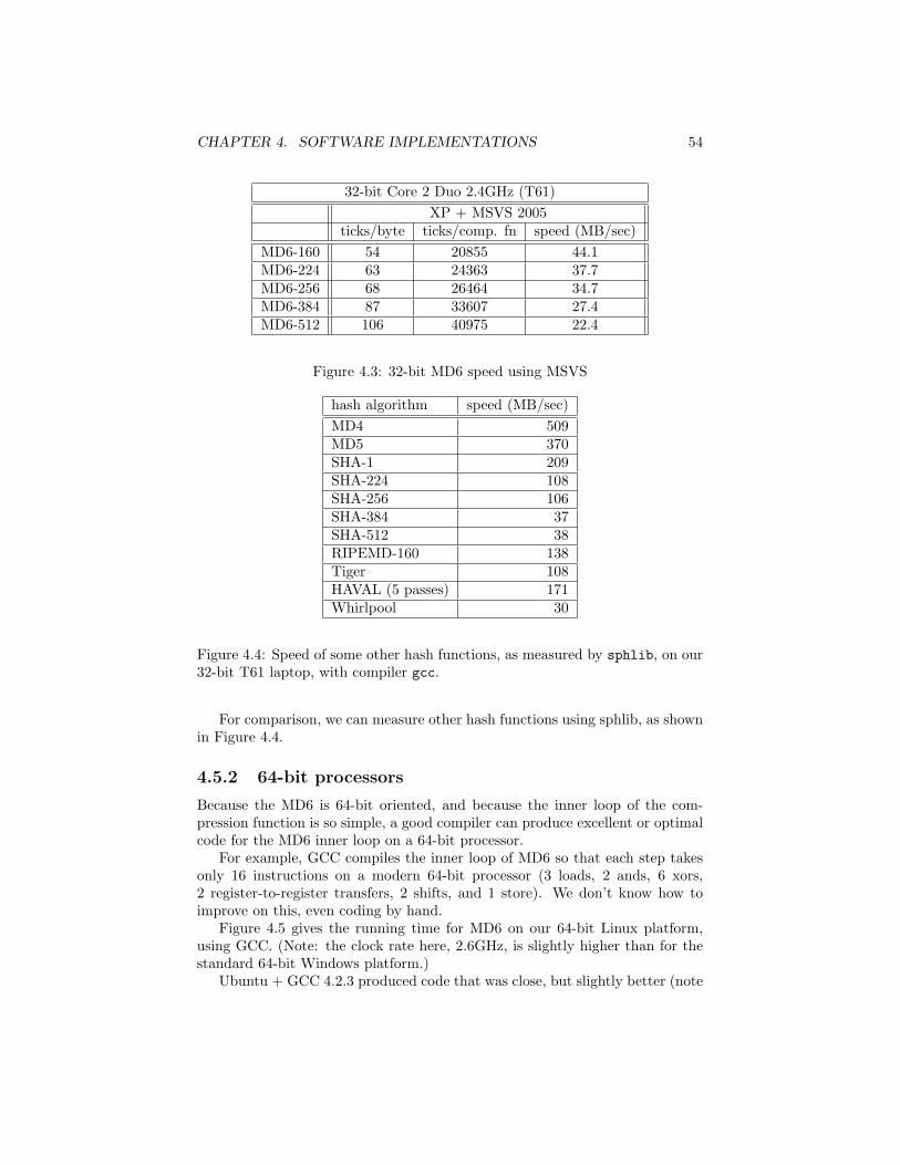
CHAPTER 4. SOFTWARE IMPLEMENTATIONS 54
32-bit Core 2 Duo 2.4GHz (T61)XP + MSVS 2005
ticks/byte ticks/comp. fn speed (MB/sec)MD6-160 54 20855 44.1MD6-224 63 24363 37.7MD6-256 68 26464 34.7MD6-384 87 33607 27.4MD6-512 106 40975 22.4
Figure 4.3: 32-bit MD6 speed using MSVS
hash algorithm speed (MB/sec)MD4 509MD5 370SHA-1 209SHA-224 108SHA-256 106SHA-384 37SHA-512 38RIPEMD-160 138Tiger 108HAVAL (5 passes) 171Whirlpool 30
Figure 4.4: Speed of some other hash functions, as measured by sphlib, on our32-bit T61 laptop, with compiler gcc.
For comparison, we can measure other hash functions using sphlib, as shownin Figure 4.4.
4.5.2 64-bit processors
Because the MD6 is 64-bit oriented, and because the inner loop of the com-pression function is so simple, a good compiler can produce excellent or optimalcode for the MD6 inner loop on a 64-bit processor.
For example, GCC compiles the inner loop of MD6 so that each step takesonly 16 instructions on a modern 64-bit processor (3 loads, 2 ands, 6 xors,2 register-to-register transfers, 2 shifts, and 1 store). We don’t know how toimprove on this, even coding by hand.
Figure 4.5 gives the running time for MD6 on our 64-bit Linux platform,using GCC. (Note: the clock rate here, 2.6GHz, is slightly higher than for thestandard 64-bit Windows platform.)
Ubuntu + GCC 4.2.3 produced code that was close, but slightly better (note
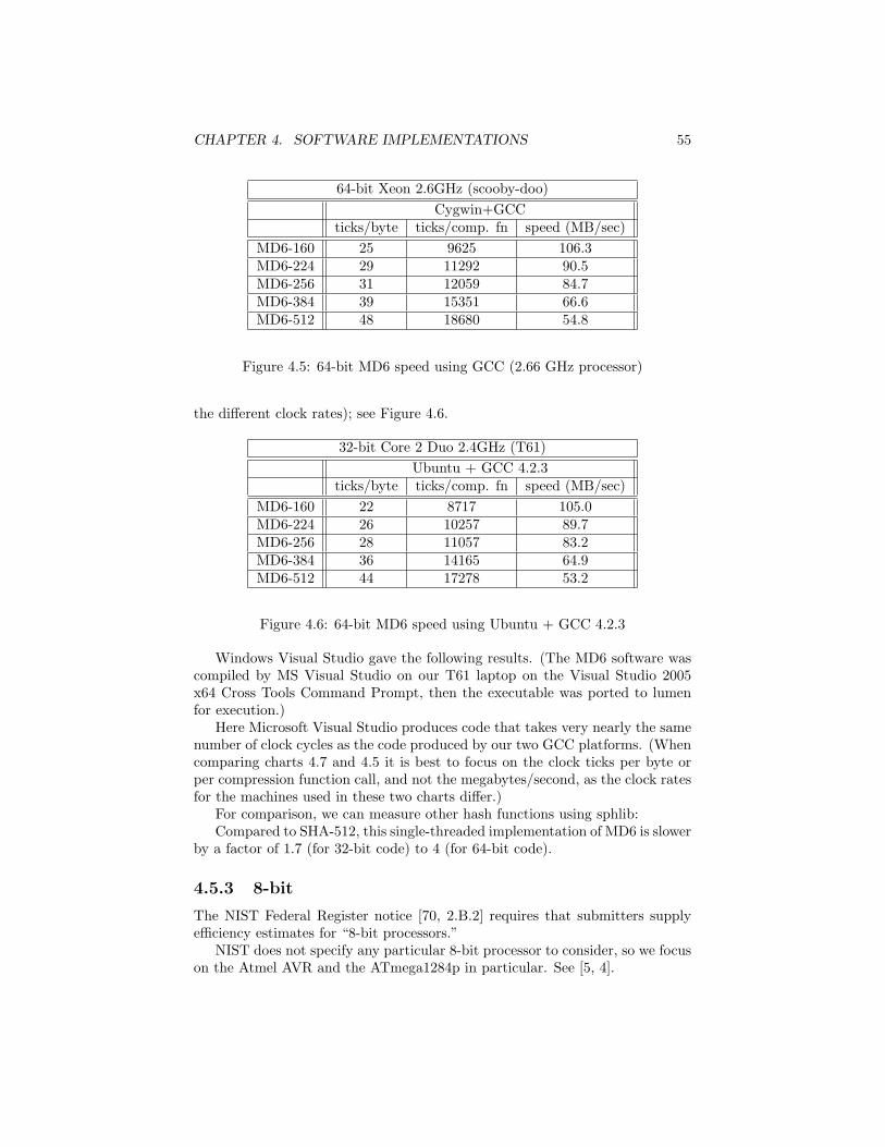
CHAPTER 4. SOFTWARE IMPLEMENTATIONS 55
64-bit Xeon 2.6GHz (scooby-doo)Cygwin+GCC
ticks/byte ticks/comp. fn speed (MB/sec)MD6-160 25 9625 106.3MD6-224 29 11292 90.5MD6-256 31 12059 84.7MD6-384 39 15351 66.6MD6-512 48 18680 54.8
Figure 4.5: 64-bit MD6 speed using GCC (2.66 GHz processor)
the different clock rates); see Figure 4.6.
32-bit Core 2 Duo 2.4GHz (T61)Ubuntu + GCC 4.2.3
ticks/byte ticks/comp. fn speed (MB/sec)MD6-160 22 8717 105.0MD6-224 26 10257 89.7MD6-256 28 11057 83.2MD6-384 36 14165 64.9MD6-512 44 17278 53.2
Figure 4.6: 64-bit MD6 speed using Ubuntu + GCC 4.2.3
Windows Visual Studio gave the following results. (The MD6 software wascompiled by MS Visual Studio on our T61 laptop on the Visual Studio 2005x64 Cross Tools Command Prompt, then the executable was ported to lumenfor execution.)
Here Microsoft Visual Studio produces code that takes very nearly the samenumber of clock cycles as the code produced by our two GCC platforms. (Whencomparing charts 4.7 and 4.5 it is best to focus on the clock ticks per byte orper compression function call, and not the megabytes/second, as the clock ratesfor the machines used in these two charts differ.)
For comparison, we can measure other hash functions using sphlib:Compared to SHA-512, this single-threaded implementation of MD6 is slower
by a factor of 1.7 (for 32-bit code) to 4 (for 64-bit code).
4.5.3 8-bit
The NIST Federal Register notice [70, 2.B.2] requires that submitters supplyefficiency estimates for “8-bit processors.”
NIST does not specify any particular 8-bit processor to consider, so we focuson the Atmel AVR and the ATmega1284p in particular. See [5, 4].
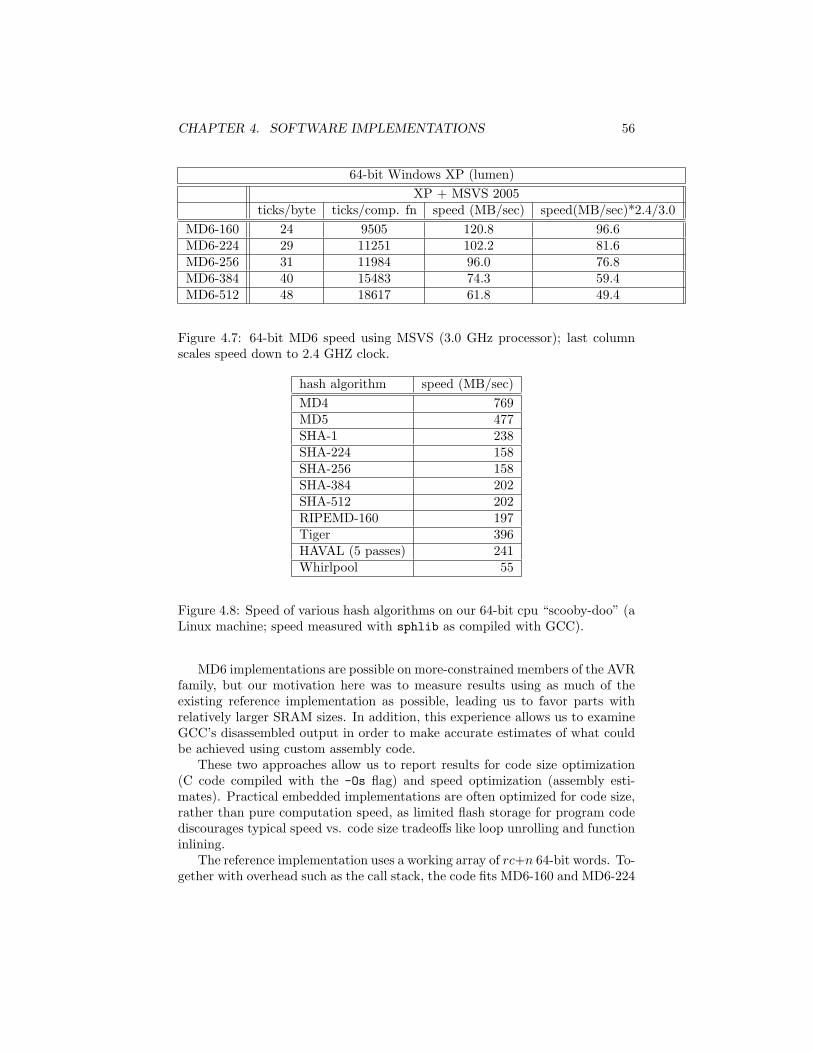
CHAPTER 4. SOFTWARE IMPLEMENTATIONS 56
64-bit Windows XP (lumen)XP + MSVS 2005
ticks/byte ticks/comp. fn speed (MB/sec) speed(MB/sec)*2.4/3.0MD6-160 24 9505 120.8 96.6MD6-224 29 11251 102.2 81.6MD6-256 31 11984 96.0 76.8MD6-384 40 15483 74.3 59.4MD6-512 48 18617 61.8 49.4
Figure 4.7: 64-bit MD6 speed using MSVS (3.0 GHz processor); last columnscales speed down to 2.4 GHZ clock.
hash algorithm speed (MB/sec)MD4 769MD5 477SHA-1 238SHA-224 158SHA-256 158SHA-384 202SHA-512 202RIPEMD-160 197Tiger 396HAVAL (5 passes) 241Whirlpool 55
Figure 4.8: Speed of various hash algorithms on our 64-bit cpu “scooby-doo” (aLinux machine; speed measured with sphlib as compiled with GCC).
MD6 implementations are possible on more-constrained members of the AVRfamily, but our motivation here was to measure results using as much of theexisting reference implementation as possible, leading us to favor parts withrelatively larger SRAM sizes. In addition, this experience allows us to examineGCC’s disassembled output in order to make accurate estimates of what couldbe achieved using custom assembly code.
These two approaches allow us to report results for code size optimization(C code compiled with the -Os flag) and speed optimization (assembly esti-mates). Practical embedded implementations are often optimized for code size,rather than pure computation speed, as limited flash storage for program codediscourages typical speed vs. code size tradeoffs like loop unrolling and functioninlining.
The reference implementation uses a working array of rc+n 64-bit words. To-gether with overhead such as the call stack, the code fits MD6-160 and MD6-224
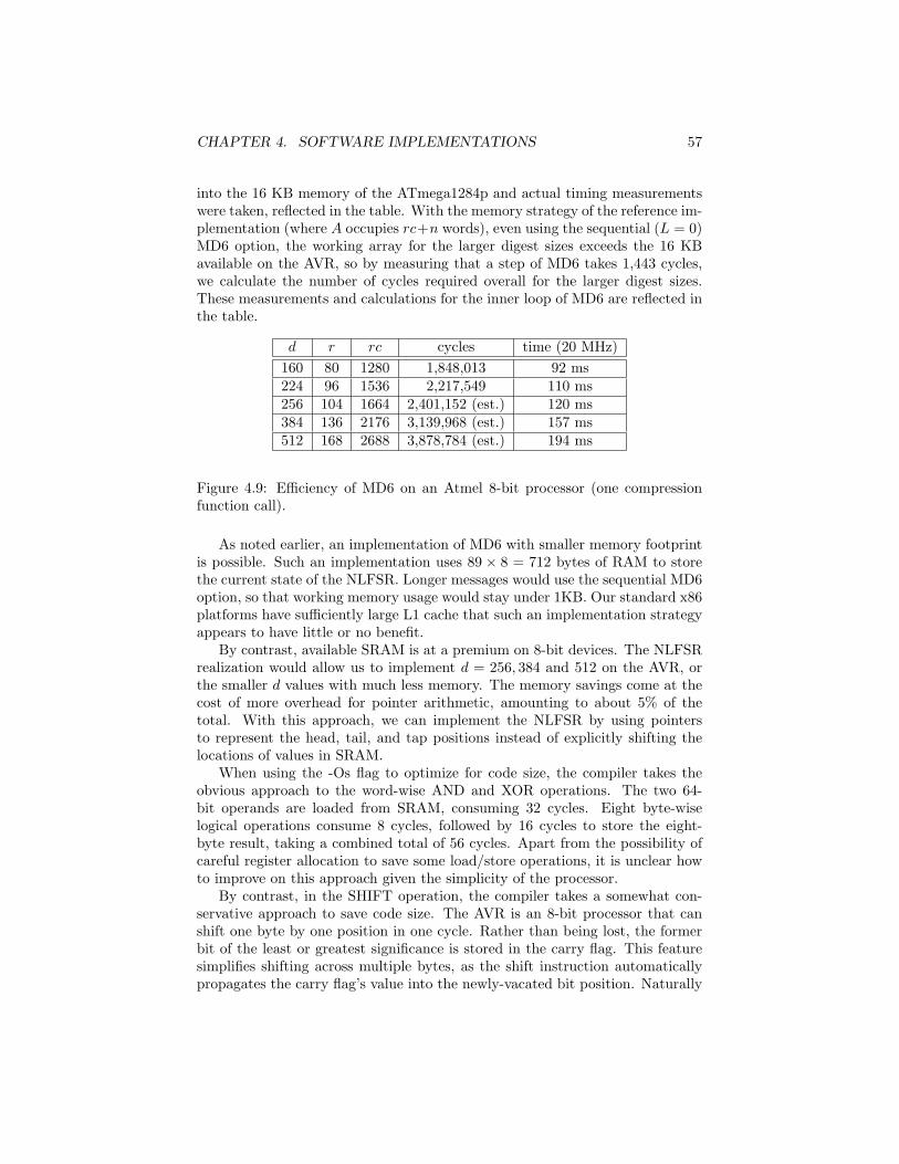
CHAPTER 4. SOFTWARE IMPLEMENTATIONS 57
into the 16 KB memory of the ATmega1284p and actual timing measurementswere taken, reflected in the table. With the memory strategy of the reference im-plementation (where A occupies rc+n words), even using the sequential (L = 0)MD6 option, the working array for the larger digest sizes exceeds the 16 KBavailable on the AVR, so by measuring that a step of MD6 takes 1,443 cycles,we calculate the number of cycles required overall for the larger digest sizes.These measurements and calculations for the inner loop of MD6 are reflected inthe table.
d r rc cycles time (20 MHz)160 80 1280 1,848,013 92 ms224 96 1536 2,217,549 110 ms256 104 1664 2,401,152 (est.) 120 ms384 136 2176 3,139,968 (est.) 157 ms512 168 2688 3,878,784 (est.) 194 ms
Figure 4.9: Efficiency of MD6 on an Atmel 8-bit processor (one compressionfunction call).
As noted earlier, an implementation of MD6 with smaller memory footprintis possible. Such an implementation uses 89 × 8 = 712 bytes of RAM to storethe current state of the NLFSR. Longer messages would use the sequential MD6option, so that working memory usage would stay under 1KB. Our standard x86platforms have sufficiently large L1 cache that such an implementation strategyappears to have little or no benefit.
By contrast, available SRAM is at a premium on 8-bit devices. The NLFSRrealization would allow us to implement d = 256, 384 and 512 on the AVR, orthe smaller d values with much less memory. The memory savings come at thecost of more overhead for pointer arithmetic, amounting to about 5% of thetotal. With this approach, we can implement the NLFSR by using pointersto represent the head, tail, and tap positions instead of explicitly shifting thelocations of values in SRAM.
When using the -Os flag to optimize for code size, the compiler takes theobvious approach to the word-wise AND and XOR operations. The two 64-bit operands are loaded from SRAM, consuming 32 cycles. Eight byte-wiselogical operations consume 8 cycles, followed by 16 cycles to store the eight-byte result, taking a combined total of 56 cycles. Apart from the possibility ofcareful register allocation to save some load/store operations, it is unclear howto improve on this approach given the simplicity of the processor.
By contrast, in the SHIFT operation, the compiler takes a somewhat con-servative approach to save code size. The AVR is an 8-bit processor that canshift one byte by one position in one cycle. Rather than being lost, the formerbit of the least or greatest significance is stored in the carry flag. This featuresimplifies shifting across multiple bytes, as the shift instruction automaticallypropagates the carry flag’s value into the newly-vacated bit position. Naturally
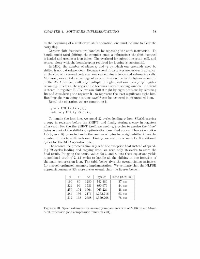
CHAPTER 4. SOFTWARE IMPLEMENTATIONS 58
at the beginning of a multi-word shift operation, one must be sure to clear thecarry flag.
Greater shift distances are handled by repeating the shift instruction. Tohandle multi-word shifting, the compiler emits a subroutine: the shift distanceis loaded and used as a loop index. The overhead for subroutine setup, call, andreturn, along with the housekeeping required for looping is substantial.
In MD6, the number of places li and ri by which our operands need beshifted is not data-dependent. Because the shift distances are known in advance,at the cost of increased code size, one can eliminate loops and subroutine calls.Moreover, we can take advantage of an optimization due to the byte-wise natureof the AVR: we can shift any multiple of eight positions merely by registerrenaming. In effect, the register file becomes a sort of sliding window: if a wordis stored in registers R0-R7, we can shift it right by eight positions by zeroizingR8 and considering the register R1 to represent the least-significant eight bits.Handling the remaining positions mod 8 can be achieved in an unrolled loop.
Recall the operation we are computing is
y = x XOR (x >> r_i);return y XOR (y << l_i);
To handle the first line, we spend 32 cycles loading x from SRAM, storinga copy in registers before the SHIFT, and finally storing a copy in registersafterward. For the the SHIFT itself, we need ri/8 cycles to zeroize the “free”bytes as part of the shift-by-8 optimization described above. Then (8− ri/8 +1)× [ri mod 8] cycles to handle the number of bytes to be right-shifted times thenumber of bits to shift each one. Finally, we need to account for 8 additionalcycles for the XOR operation itself.
The second line proceeds similarly with the exception that instead of spend-ing 32 cycles loading and copying data, we need only 16 cycles to store thefinal result. Plugging the actual values for li and ri into these equations yieldsa combined total of 2,113 cycles to handle all the shifting in one iteration ofthe main compression loop. The table below gives the overall timing estimatesfor a speed-optimized assembly implementation. We estimate that the NLFSRapproach consumes 5% more cycles overall than the figures below.
d r rc cycles time (20MHz)160 80 1280 742,480 37 ms224 96 1536 890,976 44 ms256 104 1664 965,224 48 ms384 136 2176 1,262,216 63 ms512 168 2688 1,559,208 78 ms
Figure 4.10: Speed estimates for assembly implementation of MD6 on an Atmel8-bit processor (one compression function call).
CHAPTER 4. SOFTWARE IMPLEMENTATIONS 59
4.5.3.0.1 Whither small processors? When measured by total units sold,8-bit processors are still the world’s most popular. Their low cost continuesto make them the processor of choice in embedded systems. The high salesvolumes mean that fast-paced innovation continues, especially as vendors offermore features while remaining at relatively low price points. The immense costpressures dictate that the 8-bit market will remain highly fragmented, withparts being highly optimized for a particular application.
Eight-bit processors remain popular in smart cards, for example. Given theirneed for a standardized I/O interface, custom hardware accelerators for sym-metric and public-key algorithms, and physical tamper-resistance, these devicesoften have a very different architecture and feature set than the typical micro-controller deployed in a television remote control, for instance. Because of thebroad diversity of processor architecture and instruction set, algorithm perfor-mance will vary from processor to processor. Simple things like the number ofclock cycles needed to read (or operate on) SRAM can make a big difference,making comparisons difficult. But because much of the time in the implementa-tion is spent ferrying data to and from memory, the time needed for a processor’sload-operate-store sequence (or equivalent) will make a big difference. The AVRhas a relatively fast path to memory (only two cycles), so given slower memoryaccess, an MD6 implementation would be correspondingly slower.
Product roadmaps for 8-bit microcontrollers tend to focus on the integrationinto the processor of components formerly requiring a separate chip. Obviousexamples are on-chip display-driver capabilities, with some processors now di-rectly carrying the circuitry to control a small liquid-crystal display. In addition,the communication features continue to expand. A variety of low-power wiredand wireless data transports are now available including CAN, Bluetooth, Zig-Bee, WiBree and many proprietary schemes. To better support this kind of dataI/O, some processors are gaining features like Direct Memory Access (DMA)that speed the flow of data to and from off-chip resources.
Closer to our purposes, some 8-bit microcontrollers like the AVR XMEGA(even those not packaged for inclusion in a smart card) now offer hardware DESand AES accelerators. Naturally, smart card processors have had unique needsfor both symmetric and public-key hardware acceleration as well as tamper-resistance for quite some time. The fact that these features are cropping up inmore general-purpose processors is a testament to the increasing connectivityeven among these smallest of systems.
Ultimately, in a few years’ time, we can expect hardware accelerators for thenew hash standard to appear in 8-bit processors just as AES accelerators arewidely available.
4.6 MD6 Memory Usage
The size of the MD6 state, as implemented, is 15504 bytes. Most of this is forthe stack of values: there are 29 levels to the stack, each holds 64 words of data,and each word is 8 bytes; this gives 14,848 bytes just for the stack.
CHAPTER 4. SOFTWARE IMPLEMENTATIONS 60
The reference implementation provides for handling the full maximum mes-sage length of 264 − 1 bits. Should there be a smaller limit in practice, acorrespondingly reduced stack size could be used. For example, if in an applica-tion there was a known maximum message size of 32GB (240 bits), then a stacksize of 17 levels would suffice, reducing the necessary size of the MD6 state toroughly 9K bytes.
When L = 0, so that MD6 is operating entirely sequentially, the size of MD6state is even further reduced. In this case, MD6 should be implementable usingnot much more than the size of one 89-word compression input, which is 712bytes.
4.7 Parallel Implementations
Computing platforms are quickly becoming highly parallel, as chip manufac-turers realize little more performance is available by increasing clock rates. In-creased performance is instead being obtained by utilizing increased parallelism,as through multi-core chip designs.
Indeed, typical chips may become very highly parallel, very soon.Anwar Ghoulum, at Intel’s Microprocessor Technology Lab, says “developers
should start thinking about tens, hundreds, and thousands of cores now.”Section 4.7.1 shows how the speed of MD6 can be dramatically increased by
utilizing the CILK software system for programming multicore computers.Then Section 4.7.2 shows how the speed of MD6 can be dramatically increase
by implementing MD6 on a typical graphics card (which is highly parallel in-ternally).
4.7.1 CILK Implementation
We implemented MD6 for multicore processors using the CILK extension tothe C programming language developed by Professor Charles Leiserson andcolleagues. CILK began as an MIT research project, and is now a startupcompany based in Lexington, Mass.
The CILK technology makes multicore programming quite straightforward.The CILK programmer identifies her C procedures that are to be managed bythe CILK runtime routines by the cilk keyword. She can identify procedurecalls to be potentially handled by other processors by the spawn keyword. Shesynchronizes a number of spawned procedure calls using the sync statement.Details can be found at the MIT CILK web site3 or at the company’s web site4.
Our implementation of MD6 in CILK used the layer-by-layer approach (soit assumes that the input message is available all at once). It processes eachlayer in turn, but uses parallelism to process a layer efficiently.
3http://supertech.csail.mit.edu/cilk/4http://www.cilk.com
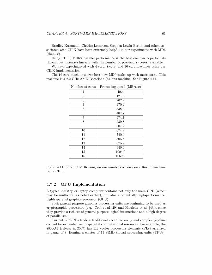
CHAPTER 4. SOFTWARE IMPLEMENTATIONS 61
Bradley Kuszmaul, Charles Leiserson, Stephen Lewin-Berlin, and others as-sociated with CILK have been extremely helpful in our experiments with MD6(thanks!).
Using CILK, MD6’s parallel performance is the best one can hope for: itsthroughput increases linearly with the number of processors (cores) available.
We have experimented with 4-core, 8-core, and 16-core machines using ourCILK implementation.
The 16-core machine shows best how MD6 scales up with more cores. Thismachine is a 2.2 GHz AMD Barcelona (64-bit) machine. See Figure 4.11.
Number of cores Processing speed (MB/sec)1 40.42 121.63 202.24 270.25 338.36 407.77 474.18 539.89 607.210 674.211 740.012 805.813 875.914 940.015 1004.016 1069.9
Figure 4.11: Speed of MD6 using various numbers of cores on a 16-core machineusing CILK.
4.7.2 GPU Implementation
A typical desktop or laptop computer contains not only the main CPU (whichmay be multicore, as noted earlier), but also a potentially high-performance,highly-parallel graphics processor (GPU).
Such general purpose graphics processing units are beginning to be used ascryptographic processors (e.g. Cool et al [29] and Harrison et al. [43]), sincethey provide a rich set of general-purpose logical instructions and a high degreeof parallelism.
Current GPGPUs trade a traditional cache hierarchy and complex pipelinecontrol for expanded vector-parallel computational resources. For example, the8800GT (release in 2007) has 112 vector processing elements (PEs) arrangedin gangs of 8, forming a cluster of 14 SIMD thread processing units (TPUs).
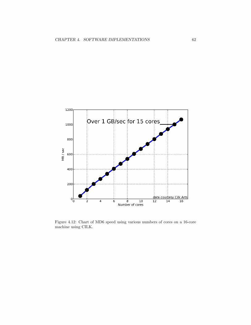
CHAPTER 4. SOFTWARE IMPLEMENTATIONS 62
Figure 4.12: Chart of MD6 speed using various numbers of cores on a 16-coremachine using CILK.
CHAPTER 4. SOFTWARE IMPLEMENTATIONS 63
The TPU operate on blocks of threads each of which must operate on thesame vector instruction. If divergent control flow exists across the threads ina TPU thread block, the PEs revert to slow serial execution. TPUs, however,may follow different control paths from one another. Unlike traditional out-of-order processors, which hide high-latency operations with instructions from thesame computation thread, the TPUs hide latency by running multiple blocksof threads in parallel. Indeed, the TPU cannot even execute back to backinstructions from the same thread block in back to back cycles – the TPU willidle if there are no other thread blocks to execute. Thus, to exploit the resourcesof the GPU fully, a program must have suffcient vector parallelism to saturatea TPU, limited control flow within the TPU, and enough data-parallel tasks tokeep all of the TPUs in the system busy.
MD6 is ideally suited to exploit the parallelism presented by such GPGPUarchitectures. The 16 steps in a compression round are vector parallel, and thecompression function itself has statically determined control flow. Since indi-vidual compression functions are data parallel, multiple compression functionsmaybe run in parallel on the processing units of the GPGPU, thereby achievinghigh GPU utilization. MD6 can achieve throughputs as high as 610 MB/s on asingle GPU,
We tested several GPU implementations by hashing a 512MB block of mem-ory. Performance was determined by measuring the wall clock time between thecompletion of data initialization until the completion of hashing. In particu-lar, heap memory allocation is not accounted for in the reported performance.Although memory allocation incurs substantial performance overhead, MD6 islikely to be used as part of a library in which the cost of memory allocation isamortized across many hash operations.
The GPU implementation of MD6 operates on the MD6 compression treein the same manner as the multicore implementation, that is layer by layer (seeSection 4.1.1.1). The routine uses the GPU to compress blocks of data, com-puting a minimum of 64 compression functions in parallel (32 kilobytes) perGPU invocation. Smaller data sizes, including the tip of the compression treeare calculated on the main system processor, which is faster than the GPU ifinsuffcient parallelism is available. In contrast to the traditional software imple-mentation detailed in Section 4.1.2 which required little manual modification toachieve good performance, a number of transformations must be made to theMD6 reference code in order to achieve any reasonable performance on the GPU.Unfortunately, many of these transformations depend on detailed knowledge ofthe GPU processor and memory architecture. The following paragraphs willpresent some details about the transformations required to achieve high GPUperformance, but may be bypassed without affecting the remaining discussion.
Running the reference implementation of MD6 on the GPU results in theabysmal compression performance of 3MB/s. The naive parallel decompositionof the code into multiple data-independent compression functions, similar tothe algorithm used in CILK, gives a low throughput of 14MB/s. The originalcompression function is not expressed in a vector parallel fashion; as such, theGPU has many idle processing elements and as a result gives low performance.
CHAPTER 4. SOFTWARE IMPLEMENTATIONS 64
Unfortunately, vectorizing the code provides a throughput of only 23 MB/s.A major performance issue with the original code is that it uses a large
array in which each element is written exacly once. While this approach isfine for a general purpose processor with a managed cache as discussed in Sec-tion 4.1.2, the GPU incurs a substantial performance penalty each time theon-board DRAM, the only place where such a large array can be stored, is ac-cessed. In MD6 compression, the ratio of computation per load is low and so theGPU is unable to hide the latency of main memory accesses with computation,resulting in severly degraded performance. To avoid this memory access penalty,the GPU implementation uses a smaller wrap-around shift register mapped inthe TPU scratch pad memory. Since vector parallel instructions may write be-yond the end of the data array, the wrap-around arrays require a halo of memoryaround them to avoid data corruption. Thus, the shift register is sized at 121words, which includes a 32 word halo. The wrap-around implementation solvesthe memory access latency problem, but introduces costly modulo arithmeticto compute array indices. However, the benefit of high memory bandwidthoutweighs the cost of modular indexing, and this implementation achieves athroughput of 140MB/s. As an aside, it might seem that increasing the shiftregister to size 128 would reduce the modulo operator to a simple right shift.However, this optimization results in an array of shift registers that does not fitin the 16KB TPU scratchpad memory.
Although modular arithmetic is needed to compute indices into the reducedshift register, the index progression is fixed and index values can be precom-puted and stored in a lookup table in scratchpad memory. This optimizationraises GPGPU thoughput to 224 MB/s. However, the table lookups still requiremodulo arithmetic operator. By removing the modulus operators and staticallyunrolling the entire compression loop, a performance of 360 MB/s was achieved.
To this point, the GPU kernel has operated on large blocks consisting ofa constant number of MD6 compression functions, but by operating the GPUat a finer granularity some speedup can be obtained. However, large scaleparallelism is required to obtain good GPU performance. MD6 is no exception- the larger the block processed, the greater the processing effciency. It wasempirically determined that 64 parallel compressions was the point at whichGPU and CPU performance were roughly equivalent. Support for smaller blocksizes increased MD6 throughput to 400 MB/s.
Modern machines have the capability to copy large pieces of physical memoryto bus devices, such as the GPU. These direct memory access or DMA transfersare high-bandwidth and may be performed in parallel with computation - eitherat the GPU or CPU. By enabling GPU DMA, a further speedup to 475 MB/swas obtained for MD6-512. Unfortunately, configuring memory for use withDMA has non-neglidgable cost. However, if MD6 were used in the contextof library, this cost would be amortized over many calls to the compressionfunction.
Utilizing these methods on the newer, faster 9800GTX card we can achieveMD6 throughput of 610 MB/s for MD6-512. We also obtain high throughputfor shorter hash lengths, as shown in Figure 4.13. In particular for extremely
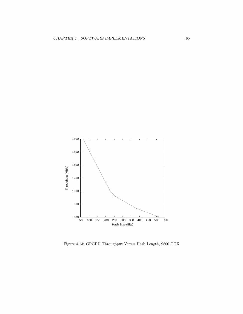
CHAPTER 4. SOFTWARE IMPLEMENTATIONS 65
600
800
1000
1200
1400
1600
1800
50 100 150 200 250 300 350 400 450 500 550
Thr
ough
put (
MB
/s)
Hash Size (Bits)
Figure 4.13: GPGPU Throughput Versus Hash Length, 9800 GTX
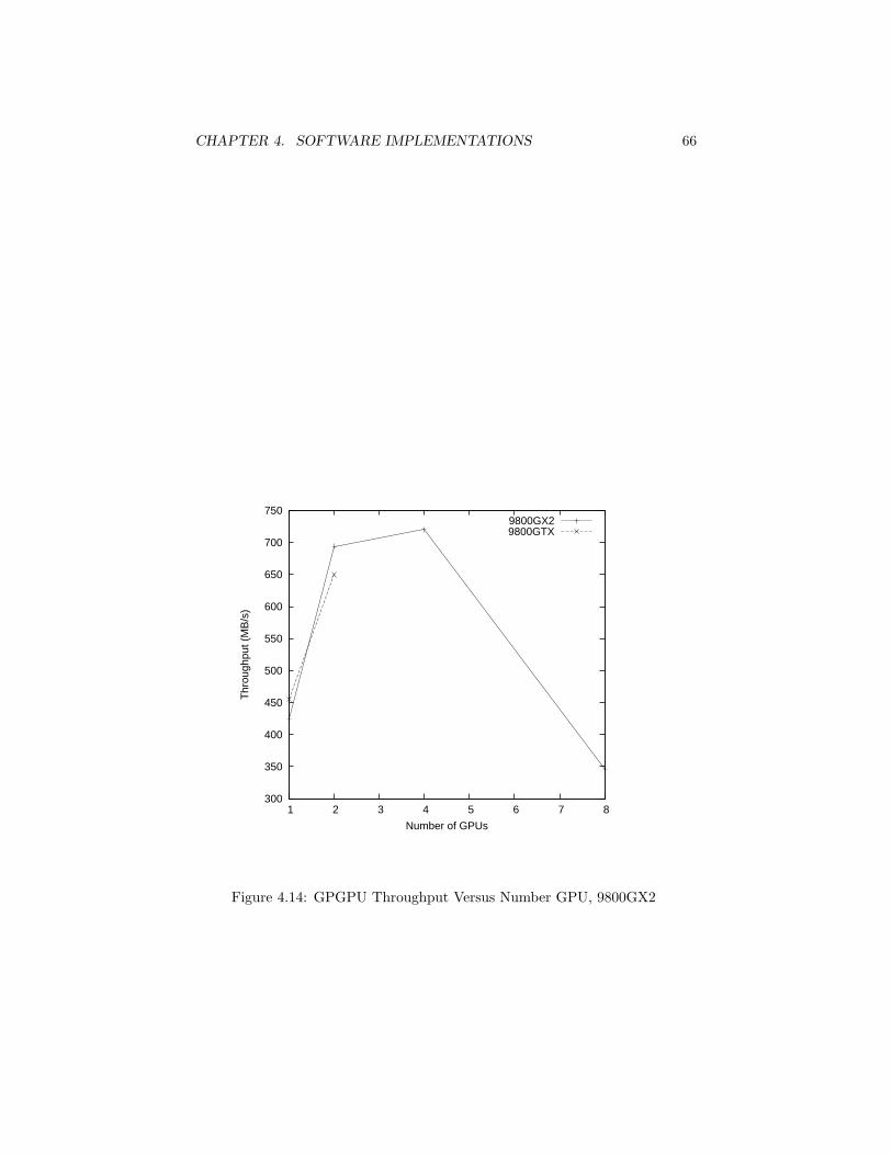
CHAPTER 4. SOFTWARE IMPLEMENTATIONS 66
300
350
400
450
500
550
600
650
700
750
1 2 3 4 5 6 7 8
Thr
ough
put (
MB
/s)
Number of GPUs
9800GX29800GTX
Figure 4.14: GPGPU Throughput Versus Number GPU, 9800GX2
CHAPTER 4. SOFTWARE IMPLEMENTATIONS 67
short hash lengths, we obtain throughputs in excess of 1600 MB/s. Althoughshort hash lengths are not crytographically interesting, their high throughputgives some notion of the maximum throughput that can be achieved with future,higher-performance GPUs.
One can install multiple graphics cards in a single desktop to obtain a higherMD6 throughput. The MD6 processing tree can be trivially partitioned andsubtrees allocated to various graphics cards within the system, theoreticallyobtaining a linear speedup in operation. The multi-GPU version of MD6 naivelypartitions the the MD6 tree into equally sized subtrees and assigns the subtreesto the available GPUs in the system. Once the subtree computation is complete,the host CPU gathers the subtree results and finishes the hash computation.
Figure 4.14 shows the MD6 throughputs achieved for MD6 on two multi-GPU platforms. The first used platform has two 9800GTX+ cards. The secondof the platforms has four 9800GX2 cards, each of which has two 9800 seriesGPUs. The second platform has more aggregate compute, although the indi-vidual 9800GTX+ GPUs are superior to the GPUs used in the 9800GX2. Forsmall increases in the number of GPUs, some performance increase is obtained.
The rapidly diminising return for using multiple graphics cards can be at-tributed to two main causes. The first is the decreased GPU efficiency due tosmaller problem size. To achieve good throughput GPUs require hundreds orthousands of threads. If the hash tree is partitioned at too fine a grain, GPUssuffer idle cycles during computation. The second is the competition for mem-ory bandwidth among the cards. Current motherboards multiplex the PCI-Ebus when multiple graphics cards are in use, decreasing the effective memorybandwidth to the all cards in the system.
4.8 Summary
MD6 has efficient software implementations on 8-bit, 32-bit, and (especially)64-bit processors, without complex optimization techniques.
Because of its tree-based mode of operation, MD6 is particularly well-suitedfor parallel implementions on multicore processors and GPU’s. Speeds of manyhundreds of megabytes per second are easily obtained, and speeds of 1-2 giga-bytes/second are very achievable.
Processor architecture is currently trending to larger numbers homogenouscores—both CPUs and GPUs are following this trend. Becuase the performanceindividual cores is not improving, the throughput of traditional sequential algo-rithms, which used to have exponential performance growth, has stagnated. Onthe other hand, highly parallel algorithms, like MD6, are likely to continue to seeimproved throughput well into the forseeable future as coarse-grained machineparallelism increases. Approximately nine months passed between the release ofthe 8800GT GPU (October 2007) and the 9800GTX GPU (July 3008), whichruns MD6 nearly 30% faster than the 8800GT; it is unlikely that any existingsequential algorithm would have demonstrated such a marked performance gainover the same time period.
Chapter 5
Hardware Implementations
Cryptographic operations are often computationally intensive – MD6 is no ex-ception. In our increasingly interconnected world, embedded platforms requirecryptographic authentication to establish trusted connections with users. How-ever, the limited general-purpose compute that is typically present in suchsystems may be incapable of satisfying the power-performance requirementsimposed on such systems. To alieviate these issues, dedicated hardware im-plementations are deployed in these devices to meet performance requirementswhile using a fraction of the power required by general-purpose compute. Recentgeneral-purpose processors [52] have included cryptographic accelerators, pre-cisely because these common operations are compute-intensive. Therefore, anystandard cryptographic operation must be efficiently implementable in hard-ware.
MD6 is highly parallelizable and exhibits strong data locality, enabling thedevelopment of efficient, extremely low power hardware implementations.
Section 5.1 first discusses our general hardware implementation strategy,paying particular attention to important hardware design tradeoffs.
We then present implementation results for a number of hardware designsfor FPGA in Section 5.2. For example, throughputs as high as 233 MB/s areobtained on a common FPGA platform while consuming only 5 Watts of power.
Section 5.3 provides some discussion of ASIC implementations; this is fol-lowed in Section 5.4 with a discussion of MD6 implementations on a custommulti-core embedded system.
5.1 Hardware Implementation
Our hardware implementation matches the version of MD6 submitted for theNIST contest. Therefore, some options and operational modes included in thedefinition of the algorithm, but not included in the proposed standard, wereomitted to reduce the complexity of the hardware. We have obtained a func-tional FPGA implementation of MD6 that achieves throughput on par with a
68
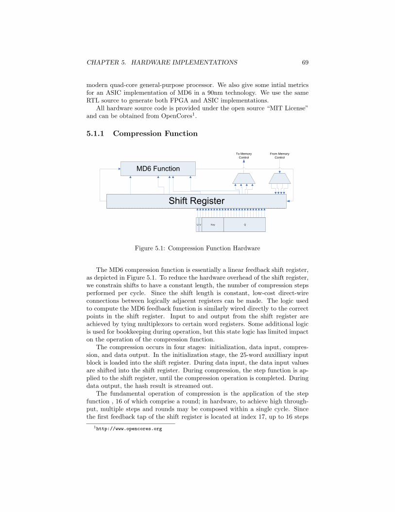
CHAPTER 5. HARDWARE IMPLEMENTATIONS 69
modern quad-core general-purpose processor. We also give some intial metricsfor an ASIC implementation of MD6 in a 90nm technology. We use the sameRTL source to generate both FPGA and ASIC implementations.
All hardware source code is provided under the open source “MIT License”and can be obtained from OpenCores1.
5.1.1 Compression Function
U V Key Q
From Memory Control
To Memory Control
Figure 5.1: Compression Function Hardware
The MD6 compression function is essentially a linear feedback shift register,as depicted in Figure 5.1. To reduce the hardware overhead of the shift register,we constrain shifts to have a constant length, the number of compression stepsperformed per cycle. Since the shift length is constant, low-cost direct-wireconnections between logically adjacent registers can be made. The logic usedto compute the MD6 feedback function is similarly wired directly to the correctpoints in the shift register. Input to and output from the shift register areachieved by tying multiplexors to certain word registers. Some additional logicis used for bookkeeping during operation, but this state logic has limited impacton the operation of the compression function.
The compression occurs in four stages: initialization, data input, compres-sion, and data output. In the initialization stage, the 25-word auxilliary inputblock is loaded into the shift register. During data input, the data input valuesare shifted into the shift register. During compression, the step function is ap-plied to the shift register, until the compression operation is completed. Duringdata output, the hash result is streamed out.
The fundamental operation of compression is the application of the stepfunction , 16 of which comprise a round; in hardware, to achieve high through-put, multiple steps and rounds may be composed within a single cycle. Sincethe first feedback tap of the shift register is located at index 17, up to 16 steps
1http://www.opencores.org
CHAPTER 5. HARDWARE IMPLEMENTATIONS 70
may be carried out in parallel, without extending the circuit critical path. Ofcourse, multiple 16-step rounds may be further composed to obtain as muchparallelism as necessary; this lengthens the critical path, introducing a designtradeoff between throughput and clock frequency.
Since the number of hash rounds is a dynamic parameter, some hash lengthsare not computable by some multiple-round per cycle implementations. Forexample, a 3-round-in-parallel implementation cannot compute a 256 bit hash(104, the number of rounds for this hash size, is not divisible by 3). Althoughthis implementation will compute the correct hash result for all round lengths,the result will have a variable location in the shift register. To generalize suchan implementation, additional control and multiplexing logic would be requiredto collect to the hash result.
5.1.2 Memory Control Logic
The hardware implementation can be viewed as a gang of compression func-tion units orchestrated by a memory controller. The function of the memorycontroller is simple: it maintains top-level status information and issues mem-ory requests to and from a memory store, or, in the case of a streaming im-plementation, I/O buffers. As in the case of software, there are two possibleimplementations of the control logic, as discussed in Section 4.1.
The layer-by-layer approach uses the least amount of logic: fewer memorypointers must be mantained, resulting in slightly less complicated control logic;this implementation is also amenable to exteremly long burst transfers, whichmay have a power-performance advantage in some systems. However, the layer-by-layer approach requires the entire message to be present in the system atthe beginning of the run, requires large amounts of memory, and exhibits poortemporal locality.
As was the case in software, the tree-building approach solves the problemsof the layer-by-layer approach at the cost of slightly increased logic area. Mor-ever, the tree building approach introduces the possiblity of a layer cache. Thelayer cache temporarily stores recently computed portions of the compressiontree, that will be used in the near future and some coherence status bits. Ascompression nodes are computed, their results are stored in the layer cache.Values in the layer cache are loaded as needed for computation. The highestlevels of the compression tree need not be stored in the cache – the performanceand power impact of caching these values is negligible.
Irrespective of architecture, the memory requests that the memory controllerissues take the form of long DMA bursts, which maximize memory bandwidth.The MD6 compression function, by design, expects input data beginning withthe least significant word and ending with the most significant word. This wordordering conforms to the burst word transfer order for all bus specificationsof which the authors are aware, and greatly simplifies the memory controllerimplementation, since a re-order buffer is not required to handle burst transfers.
Two versions of the controller were implemented. One implementation is-sues memory requests in-order. A second version of the controller adds a module
CHAPTER 5. HARDWARE IMPLEMENTATIONS 71
that does coherence bookkeeping between loads and stores, allowing loads andstores to proceed in dataflow rather than in the temporal ordering in whichthey were issued. This ordering allows some memory requests to be overlappedwith computation, since future loads may be serviced before present computa-tion has completed. Overlapped memory accesses provide a great opportunityfor system-level parallelism, but typically require extra hadware. In general,load-store bypassing also require a large amount of logic to ensure correctness,however, in the constrained case of MD6 it is fairly straightforward to trackinter-level dependencies with a handful of status bits. Our relaxed memory im-plementation requires some extra buffering to achieve full memory utilization,since requested transactions may not be immediately serviced.
5.2 FPGA
FPGAs are a reprogrammable, highly parallel substrate commonly used forprototyping hardware. Structurally, the FPGA is comprised of a grid of ho-mogenous logic slices surrounded by a configurable interconnect network. Slicesare comprised of a lookup table used to implement logic functionality and ahandful of registers used to store state. To first order, FPGA implementationarea can be estimated by the number of slices required to implement the de-sign. FPGA synthesis tools seamless map Register-Transfer-Level, i.e. Verilog,logic onto the FPGA substrate to obtain a cycle-accurate emulator of the RTLdesign. FPGAs may additionally contain small SRAM and DSP blocks whichare used to reduce the overhead of implementing common but logically complexstructures like multipliers. FPGAs are fundamentally more constrained than ap-plication specific integrated circuits (ASIC); as a result the silicon area requiredfor an FPGA implementation is larger and the maximum operational frequencyis lower than an implementation in a comparable ASIC process. NonethelessFPGAs serve as an useful platform for evaluating microarchitecture, and mostproduction RTL designs are at least partially verified on an FPGA platform.
Several implementations of MD6 were benchmarked using the Xilinx XUPdevelopment platform, which features a Xilinx Virtex-II Pro V30 FPGA. Thetest system consisted of the MD6 hardware, a PowerPC core (embedded in thFPGA), and a DDR DRAM. The PowerPC served to orchestrate the otherhardware and to provide some debugging capacity. All hardware componentsin the system were run at 100 MHz. All synthesis results were obtained usingSynopsis Synplify Pro for synthesis and the Xilinx PAR tool for backend placeand route.
The hardware was benchmarked by writing a memory array to the DRAMmemory, and then invoking a driver to begin the hardware hash. The result ofthe hash was then verified against the reference software implementation. Allreported benchmark statistics are derived from hardware performance registersembedded in the MD6 FPGA design. Although the harware was tested withmany bit lengths to ensure the correctness of the implementation, only wholeblock results are reported here, since partial blocks effectively take the same
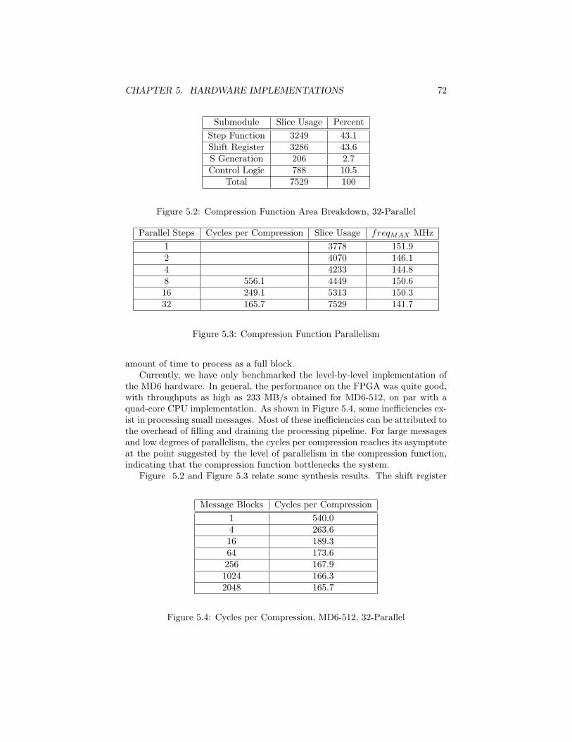
CHAPTER 5. HARDWARE IMPLEMENTATIONS 72
Submodule Slice Usage PercentStep Function 3249 43.1Shift Register 3286 43.6S Generation 206 2.7Control Logic 788 10.5
Total 7529 100
Figure 5.2: Compression Function Area Breakdown, 32-Parallel
Parallel Steps Cycles per Compression Slice Usage freqMAX MHz1 3778 151.92 4070 146.14 4233 144.88 556.1 4449 150.616 249.1 5313 150.332 165.7 7529 141.7
Figure 5.3: Compression Function Parallelism
amount of time to process as a full block.Currently, we have only benchmarked the level-by-level implementation of
the MD6 hardware. In general, the performance on the FPGA was quite good,with throughputs as high as 233 MB/s obtained for MD6-512, on par with aquad-core CPU implementation. As shown in Figure 5.4, some inefficiencies ex-ist in processing small messages. Most of these inefficiencies can be attributed tothe overhead of filling and draining the processing pipeline. For large messagesand low degrees of parallelism, the cycles per compression reaches its asymptoteat the point suggested by the level of parallelism in the compression function,indicating that the compression function bottlenecks the system.
Figure 5.2 and Figure 5.3 relate some synthesis results. The shift register
Message Blocks Cycles per Compression1 540.04 263.616 189.364 173.6256 167.91024 166.32048 165.7
Figure 5.4: Cycles per Compression, MD6-512, 32-Parallel
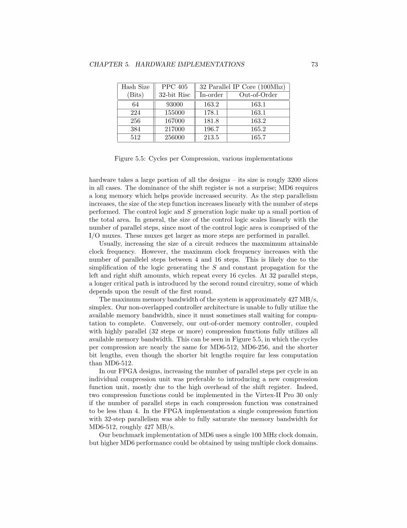
CHAPTER 5. HARDWARE IMPLEMENTATIONS 73
Hash Size PPC 405 32 Parallel IP Core (100Mhz)(Bits) 32-bit Risc In-order Out-of-Order
64 93000 163.2 163.1224 155000 178.1 163.1256 167000 181.8 163.2384 217000 196.7 165.2512 256000 213.5 165.7
Figure 5.5: Cycles per Compression, various implementations
hardware takes a large portion of all the designs – its size is rougly 3200 slicesin all cases. The dominance of the shift register is not a surprise; MD6 requiresa long memory which helps provide increased security. As the step parallelismincreases, the size of the step function increases linearly with the number of stepsperformed. The control logic and S generation logic make up a small portion ofthe total area. In general, the size of the control logic scales linearly with thenumber of parallel steps, since most of the control logic area is comprised of theI/O muxes. These muxes get larger as more steps are performed in parallel.
Usually, increasing the size of a circuit reduces the maxmimum attainableclock frequency. However, the maximum clock frequency increases with thenumber of parallelel steps between 4 and 16 steps. This is likely due to thesimplification of the logic generating the S and constant propagation for theleft and right shift amounts, which repeat every 16 cycles. At 32 parallel steps,a longer critical path is introduced by the second round circuitry, some of whichdepends upon the result of the first round.
The maximum memory bandwidth of the system is approximately 427 MB/s,simplex. Our non-overlapped controller architecture is unable to fully utilize theavailable memory bandwidth, since it must sometimes stall waiting for compu-tation to complete. Conversely, our out-of-order memory controller, coupledwith highly parallel (32 steps or more) compression functions fully utilizes allavailable memory bandwidth. This can be seen in Figure 5.5, in which the cyclesper compression are nearly the same for MD6-512, MD6-256, and the shorterbit lengths, even though the shorter bit lengths require far less computationthan MD6-512.
In our FPGA designs, increasing the number of parallel steps per cycle in anindividual compression unit was preferable to introducing a new compressionfunction unit, mostly due to the high overhead of the shift register. Indeed,two compression functions could be implemented in the Virtex-II Pro 30 onlyif the number of parallel steps in each compression function was constrainedto be less than 4. In the FPGA implementation a single compression functionwith 32-step parallelism was able to fully saturate the memory bandwidth forMD6-512, roughly 427 MB/s.
Our benchmark implementation of MD6 uses a single 100 MHz clock domain,but higher MD6 performance could be obtained by using multiple clock domains.
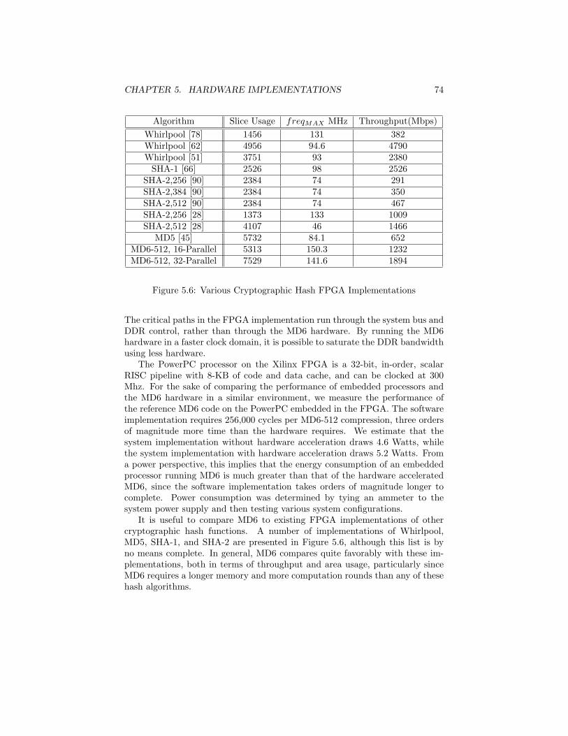
CHAPTER 5. HARDWARE IMPLEMENTATIONS 74
Algorithm Slice Usage freqMAX MHz Throughput(Mbps)Whirlpool [78] 1456 131 382Whirlpool [62] 4956 94.6 4790Whirlpool [51] 3751 93 2380
SHA-1 [66] 2526 98 2526SHA-2,256 [90] 2384 74 291SHA-2,384 [90] 2384 74 350SHA-2,512 [90] 2384 74 467SHA-2,256 [28] 1373 133 1009SHA-2,512 [28] 4107 46 1466
MD5 [45] 5732 84.1 652MD6-512, 16-Parallel 5313 150.3 1232MD6-512, 32-Parallel 7529 141.6 1894
Figure 5.6: Various Cryptographic Hash FPGA Implementations
The critical paths in the FPGA implementation run through the system bus andDDR control, rather than through the MD6 hardware. By running the MD6hardware in a faster clock domain, it is possible to saturate the DDR bandwidthusing less hardware.
The PowerPC processor on the Xilinx FPGA is a 32-bit, in-order, scalarRISC pipeline with 8-KB of code and data cache, and can be clocked at 300Mhz. For the sake of comparing the performance of embedded processors andthe MD6 hardware in a similar environment, we measure the performance ofthe reference MD6 code on the PowerPC embedded in the FPGA. The softwareimplementation requires 256,000 cycles per MD6-512 compression, three ordersof magnitude more time than the hardware requires. We estimate that thesystem implementation without hardware acceleration draws 4.6 Watts, whilethe system implementation with hardware acceleration draws 5.2 Watts. Froma power perspective, this implies that the energy consumption of an embeddedprocessor running MD6 is much greater than that of the hardware acceleratedMD6, since the software implementation takes orders of magnitude longer tocomplete. Power consumption was determined by tying an ammeter to thesystem power supply and then testing various system configurations.
It is useful to compare MD6 to existing FPGA implementations of othercryptographic hash functions. A number of implementations of Whirlpool,MD5, SHA-1, and SHA-2 are presented in Figure 5.6, although this list is byno means complete. In general, MD6 compares quite favorably with these im-plementations, both in terms of throughput and area usage, particularly sinceMD6 requires a longer memory and more computation rounds than any of thesehash algorithms.
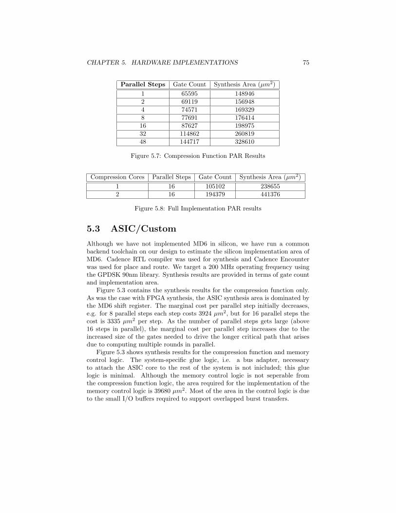
CHAPTER 5. HARDWARE IMPLEMENTATIONS 75
Parallel Steps Gate Count Synthesis Area (µm2)1 65595 1489462 69119 1569484 74571 1693298 77691 17641416 87627 19897532 114862 26081948 144717 328610
Figure 5.7: Compression Function PAR Results
Compression Cores Parallel Steps Gate Count Synthesis Area (µm2)1 16 105102 2386552 16 194379 441376
Figure 5.8: Full Implementation PAR results
5.3 ASIC/Custom
Although we have not implemented MD6 in silicon, we have run a commonbackend toolchain on our design to estimate the silicon implementation area ofMD6. Cadence RTL compiler was used for synthesis and Cadence Encounterwas used for place and route. We target a 200 MHz operating frequency usingthe GPDSK 90nm library. Synthesis results are provided in terms of gate countand implementation area.
Figure 5.3 contains the synthesis results for the compression function only.As was the case with FPGA synthesis, the ASIC synthesis area is dominated bythe MD6 shift register. The marginal cost per parallel step initially decreases,e.g. for 8 parallel steps each step costs 3924 µm2, but for 16 parallel steps thecost is 3335 µm2 per step. As the number of parallel steps gets large (above16 steps in parallel), the marginal cost per parallel step increases due to theincreased size of the gates needed to drive the longer critical path that arisesdue to computing multiple rounds in parallel.
Figure 5.3 shows synthesis results for the compression function and memorycontrol logic. The system-specific glue logic, i.e. a bus adapter, necessaryto attach the ASIC core to the rest of the system is not inicluded; this gluelogic is minimal. Although the memory control logic is not seperable fromthe compression function logic, the area required for the implementation of thememory control logic is 39680 µm2. Most of the area in the control logic is dueto the small I/O buffers required to support overlapped burst transfers.
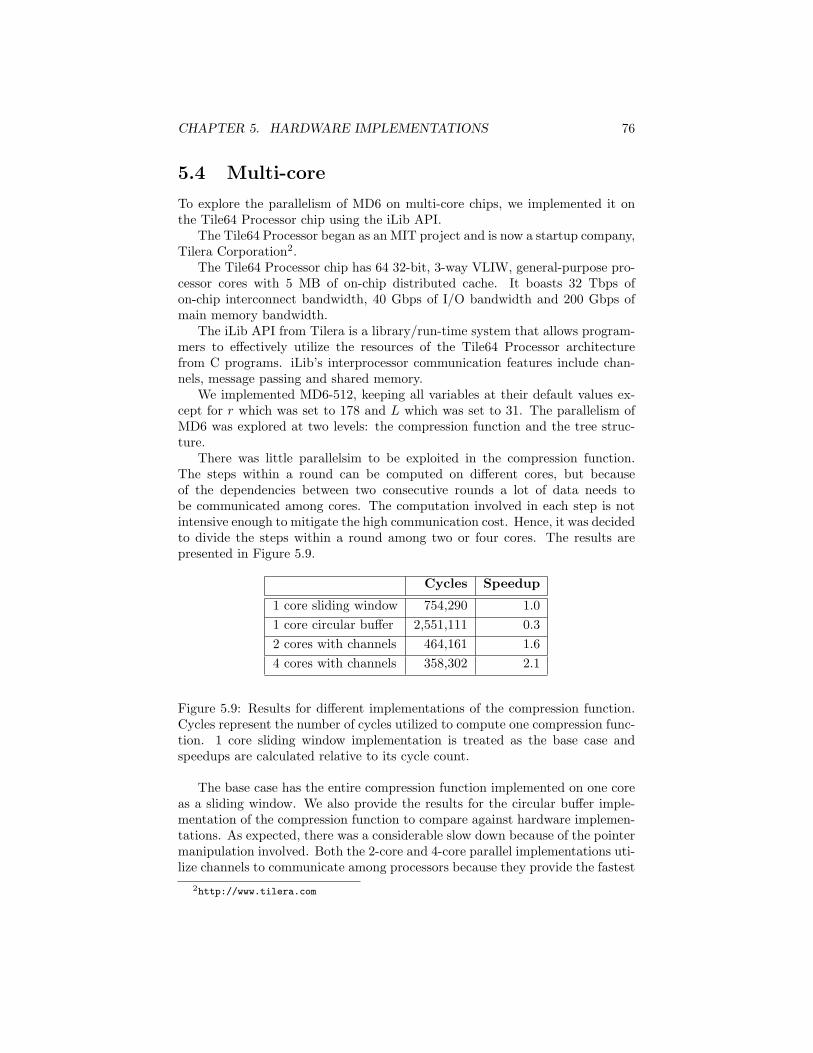
CHAPTER 5. HARDWARE IMPLEMENTATIONS 76
5.4 Multi-core
To explore the parallelism of MD6 on multi-core chips, we implemented it onthe Tile64 Processor chip using the iLib API.
The Tile64 Processor began as an MIT project and is now a startup company,Tilera Corporation2.
The Tile64 Processor chip has 64 32-bit, 3-way VLIW, general-purpose pro-cessor cores with 5 MB of on-chip distributed cache. It boasts 32 Tbps ofon-chip interconnect bandwidth, 40 Gbps of I/O bandwidth and 200 Gbps ofmain memory bandwidth.
The iLib API from Tilera is a library/run-time system that allows program-mers to effectively utilize the resources of the Tile64 Processor architecturefrom C programs. iLib’s interprocessor communication features include chan-nels, message passing and shared memory.
We implemented MD6-512, keeping all variables at their default values ex-cept for r which was set to 178 and L which was set to 31. The parallelism ofMD6 was explored at two levels: the compression function and the tree struc-ture.
There was little parallelsim to be exploited in the compression function.The steps within a round can be computed on different cores, but becauseof the dependencies between two consecutive rounds a lot of data needs tobe communicated among cores. The computation involved in each step is notintensive enough to mitigate the high communication cost. Hence, it was decidedto divide the steps within a round among two or four cores. The results arepresented in Figure 5.9.
Cycles Speedup
1 core sliding window 754,290 1.01 core circular buffer 2,551,111 0.32 cores with channels 464,161 1.64 cores with channels 358,302 2.1
Figure 5.9: Results for different implementations of the compression function.Cycles represent the number of cycles utilized to compute one compression func-tion. 1 core sliding window implementation is treated as the base case andspeedups are calculated relative to its cycle count.
The base case has the entire compression function implemented on one coreas a sliding window. We also provide the results for the circular buffer imple-mentation of the compression function to compare against hardware implemen-tations. As expected, there was a considerable slow down because of the pointermanipulation involved. Both the 2-core and 4-core parallel implementations uti-lize channels to communicate among processors because they provide the fastest
2http://www.tilera.com
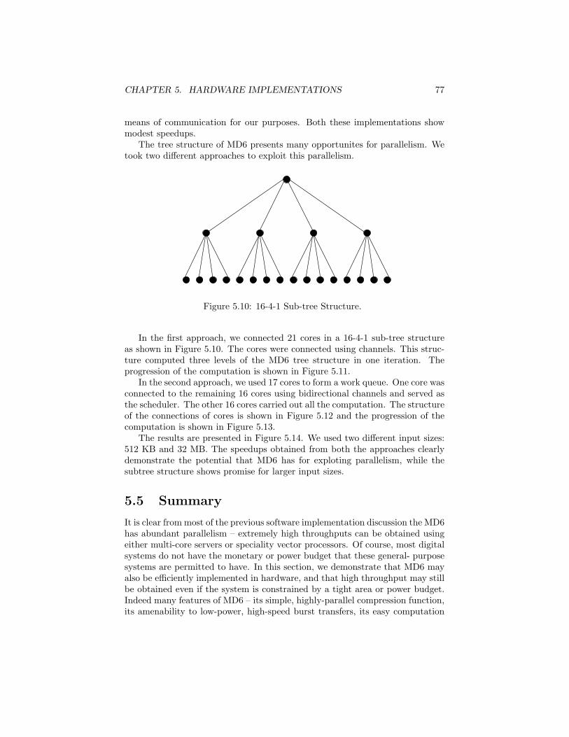
CHAPTER 5. HARDWARE IMPLEMENTATIONS 77
means of communication for our purposes. Both these implementations showmodest speedups.
The tree structure of MD6 presents many opportunites for parallelism. Wetook two different approaches to exploit this parallelism.
Figure 5.10: 16-4-1 Sub-tree Structure.
In the first approach, we connected 21 cores in a 16-4-1 sub-tree structureas shown in Figure 5.10. The cores were connected using channels. This struc-ture computed three levels of the MD6 tree structure in one iteration. Theprogression of the computation is shown in Figure 5.11.
In the second approach, we used 17 cores to form a work queue. One core wasconnected to the remaining 16 cores using bidirectional channels and served asthe scheduler. The other 16 cores carried out all the computation. The structureof the connections of cores is shown in Figure 5.12 and the progression of thecomputation is shown in Figure 5.13.
The results are presented in Figure 5.14. We used two different input sizes:512 KB and 32 MB. The speedups obtained from both the approaches clearlydemonstrate the potential that MD6 has for exploting parallelism, while thesubtree structure shows promise for larger input sizes.
5.5 Summary
It is clear from most of the previous software implementation discussion the MD6has abundant parallelism – extremely high throughputs can be obtained usingeither multi-core servers or speciality vector processors. Of course, most digitalsystems do not have the monetary or power budget that these general- purposesystems are permitted to have. In this section, we demonstrate that MD6 mayalso be efficiently implemented in hardware, and that high throughput may stillbe obtained even if the system is constrained by a tight area or power budget.Indeed many features of MD6 – its simple, highly-parallel compression function,its amenability to low-power, high-speed burst transfers, its easy computation
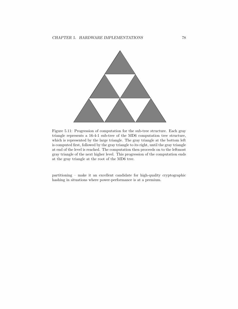
CHAPTER 5. HARDWARE IMPLEMENTATIONS 78
Figure 5.11: Progression of computation for the sub-tree structure. Each graytriangle represents a 16-4-1 sub-tree of the MD6 computation tree structure,which is represented by the large triangle. The gray triangle at the bottom leftis computed first, followed by the gray triangle to its right, until the gray triangleat end of the level is reached. The computation then proceeds on to the leftmostgray triangle of the next higher level. This progression of the computation endsat the gray triangle at the root of the MD6 tree.
partitioning – make it an excellent candidate for high-quality cryptographichashing in situations where power-performance is at a premium.
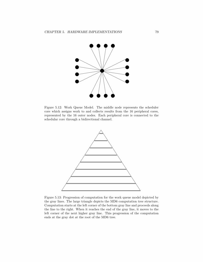
CHAPTER 5. HARDWARE IMPLEMENTATIONS 79
Figure 5.12: Work Queue Model. The middle node represents the schedulercore which assigns work to and collects results from the 16 peripheral cores,represented by the 16 outer nodes. Each peripheral core is connected to theschedular core through a bidirectional channel.
Figure 5.13: Progression of computation for the work queue model depicted bythe gray lines. The large triangle depicts the MD6 computation tree structure.Computation starts at the left corner of the bottom gray line and proceeds alongthe line to the right. When it reaches the end of the gray line, it moves to theleft corner of the next higher gray line. This progression of the computationends at the gray dot at the root of the MD6 tree.
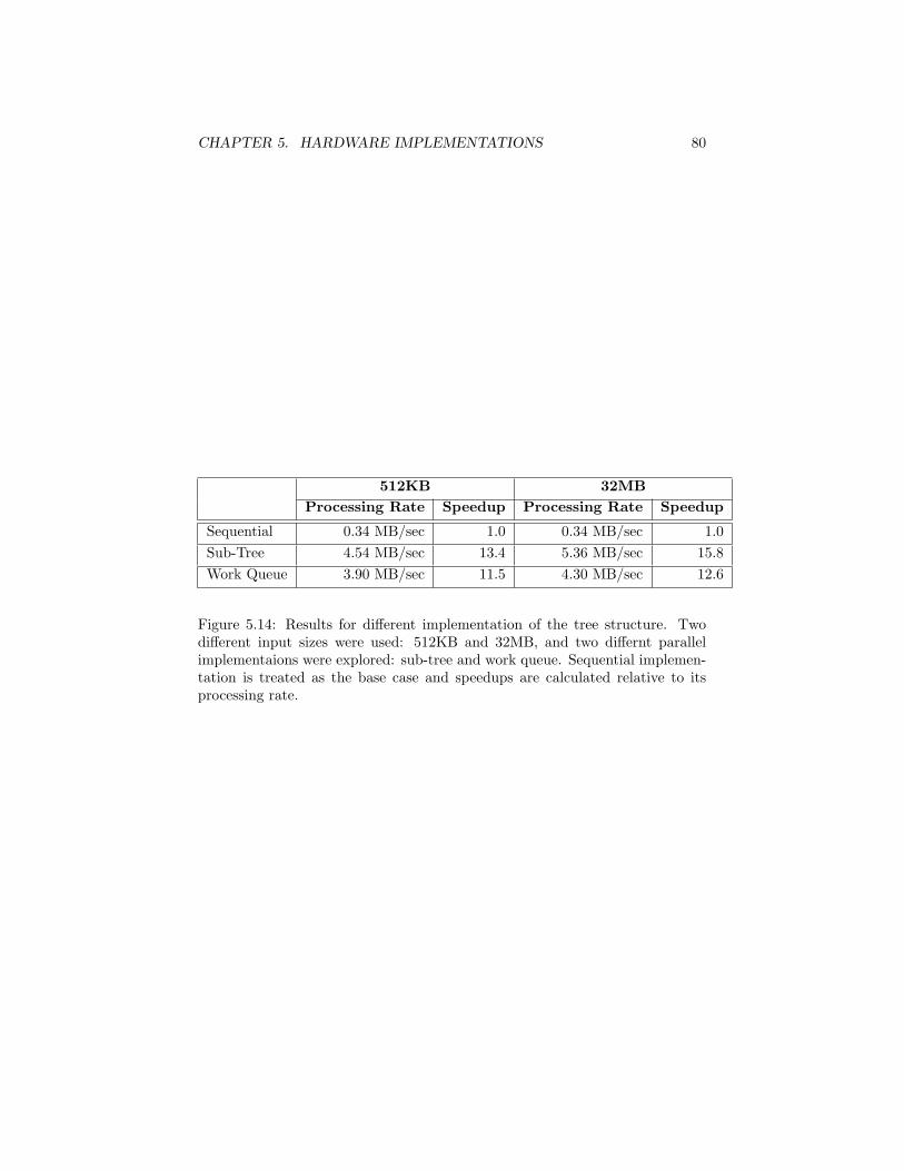
CHAPTER 5. HARDWARE IMPLEMENTATIONS 80
512KB 32MBProcessing Rate Speedup Processing Rate Speedup
Sequential 0.34 MB/sec 1.0 0.34 MB/sec 1.0Sub-Tree 4.54 MB/sec 13.4 5.36 MB/sec 15.8Work Queue 3.90 MB/sec 11.5 4.30 MB/sec 12.6
Figure 5.14: Results for different implementation of the tree structure. Twodifferent input sizes were used: 512KB and 32MB, and two differnt parallelimplementaions were explored: sub-tree and work queue. Sequential implemen-tation is treated as the base case and speedups are calculated relative to itsprocessing rate.
Chapter 6
Compression FunctionSecurity
This chapter analyzes the security of the MD6 compression function. Sincethe compression function is the “heart” of a hash function, it is importantto investigate its security from all possible angles. This chapter does so forthe MD6 compression function, looking at theoretical foundations, statisticalattacks, algebraic attacks, SAT-solver attacks, reductions, etc. MD6 stands upvery well; we were not able to discern any significant weakness in the design ofthe MD6 compression function.
Section 6.1 provides theoretical support for the architecture of the MD6compression function, which can be viewed both as a blockcipher-based hashfunction, or a permutation-based hash function. This section proves that theMD6 compression function is indifferentiable from a random oracle—a majorconfirmation of the soundness of the MD6 compression function design.
Section 6.2 discusses the choice of the constants in MD6, and their securityimplications. The use of the programs tapopt.c and shiftopt.c to choose theMD6 tap positions and shift amounts is explained. This section also reviews the“avalanche properties” of MD6, and discusses how MD6 is designed in a waythat makes “trapdoors” extremely implausible.
Section 6.3 reviews evidence presented for the collision-resistance of the MD6compression function.
Section 6.4 similarly reviews evidence for the preimage-resistance of theMD6 compression function, while Section 6.5 presents evidence for the secondpreimage-resistance of the MD6 compression function.
Section 6.6 discusses the pseudorandomness of the MD6 compression func-tion. This includes results from a standard statistical test suite (testu01) aswell as results from another heuristic statistical test we designed for testing theMD6 hash function.
Section 6.7 discusses evidence for the unpredictability of the MD6 compres-sion function (thus making it useful for message authentication codes).
81
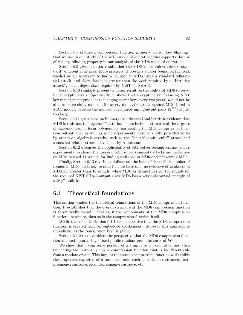
CHAPTER 6. COMPRESSION FUNCTION SECURITY 82
Section 6.8 studies a compression function property called “key blinding”that we use in our study of the MD6 mode of operation; this supports the useof the key-blinding property in our analysis of the MD6 mode of operation.
Section 6.9 gives a major result, that the MD6 is not vulnerable to “stan-dard” differential attacks. More precisely, it presents a lower bound on the workneeded by an adversary to find a collision in MD6 using a standard differen-tial attack, and show that it is greater than the work required by a “birthdayattack”, for all digest sizes required by NIST for SHA-3.
Section 6.10 similarly presents a major result on the ability of MD6 to resistlinear cryptanalysis. Specifically, it shows that a cryptanalyst following NISTkey management guidelines (changing secret keys every two years) would not beable to successfully mount a linear cryptanalytic attack against MD6 (used inMAC mode), because the number of required input/output pairs (2210) is justtoo large.
Section 6.11 gives some preliminary experimental and heuristic evidence thatMD6 is resistant to “algebraic” attacks. These include estimates of the degreesof algebraic normal form polynomials representing the MD6 compression func-tion output bits, as well as some experimental results kindly provided to usby others on algebraic attacks, such as the Dinur/Shamir “cube” attack andsomewhat related attacks developed by Aumasson.
Section 6.12 discusses the applicability of SAT solver techniques, and showsexperimental evidence that generic SAT solver (minisat) attacks are ineffectiveon MD6 beyond 11 rounds for finding collisions in MD6 or for inverting MD6.
Finally, Section 6.13 revisits and discusses the issue of the default number ofrounds in MD6. In brief, we note that we have seen no evidence of weakness inMD6 for greater than 18 rounds, while MD6 as defined has 96–168 rounds forthe required NIST SHA-3 output sizes; MD6 has a very substantial “margin ofsafety” built-in.
6.1 Theoretical foundations
This section studies the theoretical foundations of the MD6 compression func-tion. It establishes that the overall structure of the MD6 compression functionis theoretically sound. That is, if the components of the MD6 compressionfunction are secure, then so is the compression function itself.
We first consider in Section 6.1.1 the perspective that the MD6 compressionfunction is created from an embedded blockcipher. However this approach isunrealistic, as the “encryption key” is public.
Section 6.1.2 thus considers the perspective that the MD6 compression func-tion is based upon a single fixed public random permutation π of Wn.
We show that fixing some portion of π’s input to a fixed value, and thentruncating the output, yields a compression function that is indifferentiablefrom a random oracle. This implies that such a compression function will exhibitthe properties expected of a random oracle, such as collision-resistance, first-preimage resistance, second-preimage-resistance, etc.
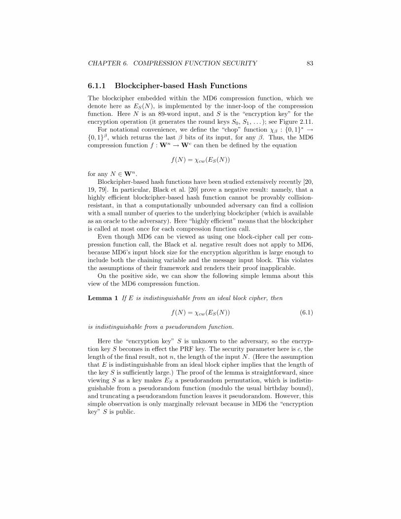
CHAPTER 6. COMPRESSION FUNCTION SECURITY 83
6.1.1 Blockcipher-based Hash Functions
The blockcipher embedded within the MD6 compression function, which wedenote here as ES(N), is implemented by the inner-loop of the compressionfunction. Here N is an 89-word input, and S is the “encryption key” for theencryption operation (it generates the round keys S0, S1, . . . ); see Figure 2.11.
For notational convenience, we define the “chop” function χβ : {0, 1}∗ →{0, 1}β , which returns the last β bits of its input, for any β. Thus, the MD6compression function f : Wn →Wc can then be defined by the equation
f(N) = χcw(ES(N))
for any N ∈Wn.Blockcipher-based hash functions have been studied extensively recently [20,
19, 79]. In particular, Black et al. [20] prove a negative result: namely, that ahighly efficient blockcipher-based hash function cannot be provably collision-resistant, in that a computationally unbounded adversary can find a collisionwith a small number of queries to the underlying blockcipher (which is availableas an oracle to the adversary). Here “highly efficient” means that the blockcipheris called at most once for each compression function call.
Even though MD6 can be viewed as using one block-cipher call per com-pression function call, the Black et al. negative result does not apply to MD6,because MD6’s input block size for the encryption algorithm is large enough toinclude both the chaining variable and the message input block. This violatesthe assumptions of their framework and renders their proof inapplicable.
On the positive side, we can show the following simple lemma about thisview of the MD6 compression function.
Lemma 1 If E is indistinguishable from an ideal block cipher, then
f(N) = χcw(ES(N)) (6.1)
is indistinguishable from a pseudorandom function.
Here the “encryption key” S is unknown to the adversary, so the encryp-tion key S becomes in effect the PRF key. The security parameter here is c, thelength of the final result, not n, the length of the input N . (Here the assumptionthat E is indistinguishable from an ideal block cipher implies that the length ofthe key S is sufficiently large.) The proof of the lemma is straightforward, sinceviewing S as a key makes ES a pseudorandom permutation, which is indistin-guishable from a pseudorandom function (modulo the usual birthday bound),and truncating a pseudorandom function leaves it pseudorandom. However, thissimple observation is only marginally relevant because in MD6 the “encryptionkey” S is public.
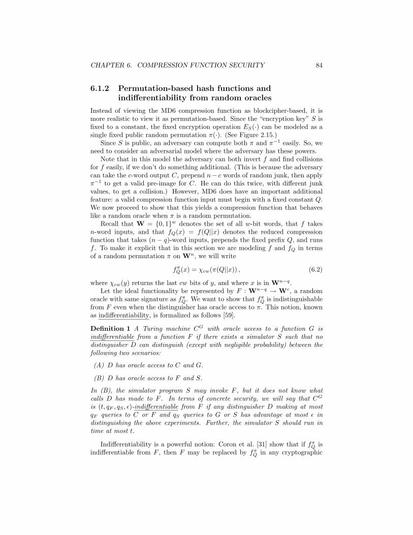
CHAPTER 6. COMPRESSION FUNCTION SECURITY 84
6.1.2 Permutation-based hash functions andindifferentiability from random oracles
Instead of viewing the MD6 compression function as blockcipher-based, it ismore realistic to view it as permutation-based. Since the “encryption key” S isfixed to a constant, the fixed encryption operation ES(·) can be modeled as asingle fixed public random permutation π(·). (See Figure 2.15.)
Since S is public, an adversary can compute both π and π−1 easily. So, weneed to consider an adversarial model where the adversary has these powers.
Note that in this model the adversary can both invert f and find collisionsfor f easily, if we don’t do something additional. (This is because the adversarycan take the c-word output C, prepend n− c words of random junk, then applyπ−1 to get a valid pre-image for C. He can do this twice, with different junkvalues, to get a collision.) However, MD6 does have an important additionalfeature: a valid compression function input must begin with a fixed constant Q.We now proceed to show that this yields a compression function that behaveslike a random oracle when π is a random permutation.
Recall that W = {0, 1}w denotes the set of all w-bit words, that f takesn-word inputs, and that fQ(x) = f(Q||x) denotes the reduced compressionfunction that takes (n− q)-word inputs, prepends the fixed prefix Q, and runsf . To make it explicit that in this section we are modeling f and fQ in termsof a random permutation π on Wn, we will write
fπQ(x) = χcw(π(Q||x)) , (6.2)
where χcw(y) returns the last cw bits of y, and where x is in Wn−q.Let the ideal functionality be represented by F : Wn−q → Wc, a random
oracle with same signature as fπQ. We want to show that fπQ is indistinguishablefrom F even when the distinguisher has oracle access to π. This notion, knownas indifferentiability, is formalized as follows [59].
Definition 1 A Turing machine CG with oracle access to a function G isindifferentiable from a function F if there exists a simulator S such that nodistinguisher D can distinguish (except with negligible probability) between thefollowing two scenarios:
(A) D has oracle access to C and G.
(B) D has oracle access to F and S.
In (B), the simulator program S may invoke F , but it does not know whatcalls D has made to F . In terms of concrete security, we will say that CG
is (t, qF , qS , ε)-indifferentiable from F if any distinguisher D making at mostqF queries to C or F and qS queries to G or S has advantage at most ε indistinguishing the above experiments. Further, the simulator S should run intime at most t.
Indifferentiability is a powerful notion: Coron et al. [31] show that if fπQ isindifferentiable from F , then F may be replaced by fπQ in any cryptographic
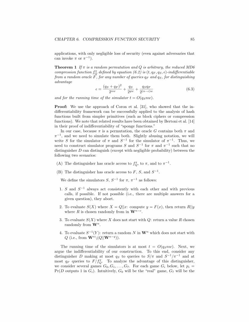
CHAPTER 6. COMPRESSION FUNCTION SECURITY 85
applications, with only negligible loss of security (even against adversaries thatcan invoke π or π−1).
Theorem 1 If π is a random permutation and Q is arbitrary, the reduced MD6compression function fπQ defined by equation (6.2) is (t, qF , qS , ε)-indifferentiablefrom a random oracle F , for any number of queries qF and qS, for distinguishingadvantage
ε =(qS + qF )2
2nw+
qS2qw
+qSqF
2(n−c)w (6.3)
and for the running time of the simulator t = O(qSnw).
Proof: We use the approach of Coron et al. [31], who showed that the in-differentiability framework can be successfully applied to the analysis of hashfunctions built from simpler primitives (such as block ciphers or compressionfunctions). We note that related results have been obtained by Bertoni et al. [14]in their proof of indifferentiability of “sponge functions.”
In our case, because π is a permutation, the oracle G contains both π andπ−1, and we need to simulate them both. Slightly abusing notation, we willwrite S for the simulator of π and S−1 for the simulator of π−1. Thus, weneed to construct simulator programs S and S−1 for π and π−1 such that nodistinguisher D can distinguish (except with negligible probability) between thefollowing two scenarios:
(A) The distinguisher has oracle access to fπQ, to π, and to π−1.
(B) The distinguisher has oracle access to F , S, and S−1.
We define the simulators S, S−1 for π, π−1 as follows:
1. S and S−1 always act consistently with each other and with previouscalls, if possible. If not possible (i.e., there are multiple answers for agiven question), they abort.
2. To evaluate S(X) where X = Q||x: compute y = F (x), then return R||ywhere R is chosen randomly from in Wn−c.
3. To evaluate S(X) where X does not start with Q: return a value R chosenrandomly from Wn.
4. To evaluate S−1(Y ): return a random N in Wn which does not start withQ (i.e., from Wn\(Q||Wn−q)).
The running time of the simulators is at most t = O(qSnw). Next, weargue the indifferentiability of our construction. To this end, consider anydistinguisher D making at most qS to queries to S/π and S−1/π−1 and atmost qF queries to F/fπQ. To analyze the advantage of this distinguisher,we consider several games G0, G1, . . . , G7. For each game Gi below, let pi =Pr(D outputs 1 in Gi). Intuitively, G0 will be the “real” game, G7 will be the
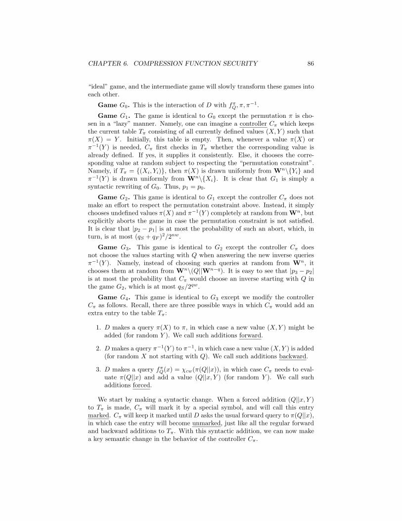
CHAPTER 6. COMPRESSION FUNCTION SECURITY 86
“ideal” game, and the intermediate game will slowly transform these games intoeach other.
Game G0. This is the interaction of D with fπQ, π, π−1.
Game G1. The game is identical to G0 except the permutation π is cho-sen in a “lazy” manner. Namely, one can imagine a controller Cπ which keepsthe current table Tπ consisting of all currently defined values (X,Y ) such thatπ(X) = Y . Initially, this table is empty. Then, whenever a value π(X) orπ−1(Y ) is needed, Cπ first checks in Tπ whether the corresponding value isalready defined. If yes, it supplies it consistently. Else, it chooses the corre-sponding value at random subject to respecting the “permutation constraint”.Namely, if Tπ = {(Xi, Yi)}, then π(X) is drawn uniformly from Wn\{Yi} andπ−1(Y ) is drawn uniformly from Wn\{Xi}. It is clear that G1 is simply asyntactic rewriting of G0. Thus, p1 = p0.
Game G2. This game is identical to G1 except the controller Cπ does notmake an effort to respect the permutation constraint above. Instead, it simplychooses undefined values π(X) and π−1(Y ) completely at random from Wn, butexplicitly aborts the game in case the permutation constraint is not satisfied.It is clear that |p2 − p1| is at most the probability of such an abort, which, inturn, is at most (qS + qF )2/2nw.
Game G3. This game is identical to G2 except the controller Cπ doesnot choose the values starting with Q when answering the new inverse queriesπ−1(Y ). Namely, instead of choosing such queries at random from Wn, itchooses them at random from Wn\(Q||Wn−q). It is easy to see that |p3 − p2|is at most the probability that Cπ would choose an inverse starting with Q inthe game G2, which is at most qS/2qw.
Game G4. This game is identical to G3 except we modify the controllerCπ as follows. Recall, there are three possible ways in which Cπ would add anextra entry to the table Tπ:
1. D makes a query π(X) to π, in which case a new value (X,Y ) might beadded (for random Y ). We call such additions forward.
2. D makes a query π−1(Y ) to π−1, in which case a new value (X,Y ) is added(for random X not starting with Q). We call such additions backward.
3. D makes a query fπQ(x) = χcw(π(Q||x)), in which case Cπ needs to eval-uate π(Q||x) and add a value (Q||x, Y ) (for random Y ). We call suchadditions forced.
We start by making a syntactic change. When a forced addition (Q||x, Y )to Tπ is made, Cπ will mark it by a special symbol, and will call this entrymarked. Cπ will keep it marked until D asks the usual forward query to π(Q||x),in which case the entry will become unmarked, just like all the regular forwardand backward additions to Tπ. With this syntactic addition, we can now makea key semantic change in the behavior of the controller Cπ.
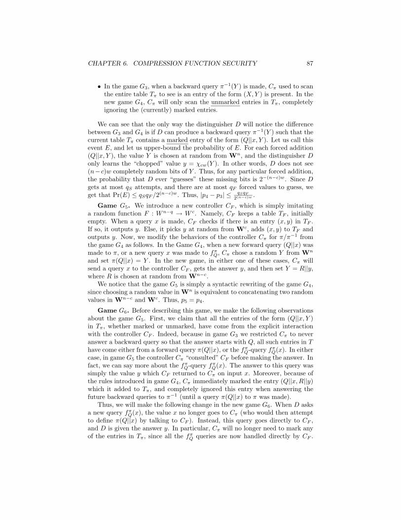
CHAPTER 6. COMPRESSION FUNCTION SECURITY 87
• In the game G3, when a backward query π−1(Y ) is made, Cπ used to scanthe entire table Tπ to see is an entry of the form (X,Y ) is present. In thenew game G4, Cπ will only scan the unmarked entries in Tπ, completelyignoring the (currently) marked entries.
We can see that the only way the distinguisher D will notice the differencebetween G3 and G4 is if D can produce a backward query π−1(Y ) such that thecurrent table Tπ contains a marked entry of the form (Q||x, Y ). Let us call thisevent E, and let us upper-bound the probability of E. For each forced addition(Q||x, Y ), the value Y is chosen at random from Wn, and the distinguisher Donly learns the “chopped” value y = χcw(Y ). In other words, D does not see(n− c)w completely random bits of Y . Thus, for any particular forced addition,the probability that D ever “guesses” these missing bits is 2−(n−c)w. Since Dgets at most qS attempts, and there are at most qF forced values to guess, weget that Pr(E) ≤ qSqF /2(n−c)w. Thus, |p4 − p3| ≤ qSqF
2(n−c)w .
Game G5. We introduce a new controller CF , which is simply imitatinga random function F : Wn−q → W c. Namely, CF keeps a table TF , initiallyempty. When a query x is made, CF checks if there is an entry (x, y) in TF .If so, it outputs y. Else, it picks y at random from Wc, adds (x, y) to TF andoutputs y. Now, we modify the behaviors of the controller Cπ for π/π−1 fromthe game G4 as follows. In the Game G4, when a new forward query (Q||x) wasmade to π, or a new query x was made to fπQ, Cπ chose a random Y from Wn
and set π(Q||x) = Y . In the new game, in either one of these cases, Cπ willsend a query x to the controller CF , gets the answer y, and then set Y = R||y,where R is chosen at random from Wn−c.
We notice that the game G5 is simply a syntactic rewriting of the game G4,since choosing a random value in Wn is equivalent to concatenating two randomvalues in Wn−c and Wc. Thus, p5 = p4.
Game G6. Before describing this game, we make the following observationsabout the game G5. First, we claim that all the entries of the form (Q||x, Y )in Tπ, whether marked or unmarked, have come from the explicit interactionwith the controller CF . Indeed, because in game G3 we restricted Cπ to neveranswer a backward query so that the answer starts with Q, all such entries in Thave come either from a forward query π(Q||x), or the fπQ-query fπQ(x). In eithercase, in game G5 the controller Cπ “consulted” CF before making the answer. Infact, we can say more about the fπQ-query fπQ(x). The answer to this query wassimply the value y which CF returned to Cπ on input x. Moreover, because ofthe rules introduced in game G4, Cπ immediately marked the entry (Q||x,R||y)which it added to Tπ, and completely ignored this entry when answering thefuture backward queries to π−1 (until a query π(Q||x) to π was made).
Thus, we will make the following change in the new game G6. When D asksa new query fπQ(x), the value x no longer goes to Cπ (who would then attemptto define π(Q||x) by talking to CF ). Instead, this query goes directly to CF ,and D is given the answer y. In particular, Cπ will no longer need to mark anyof the entries in Tπ, since all the fπQ queries are now handled directly by CF .
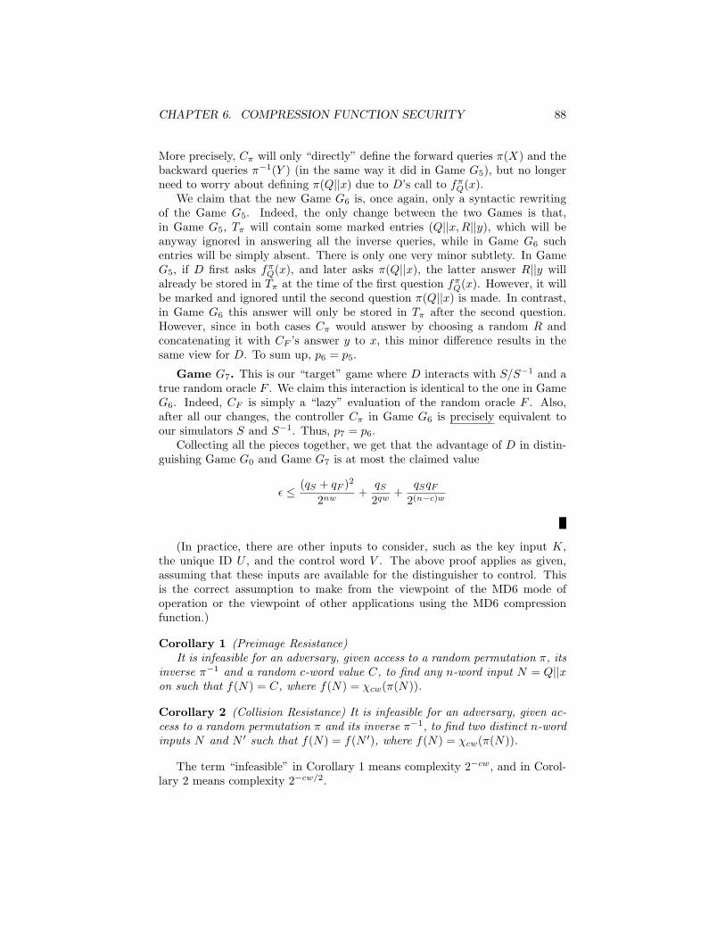
CHAPTER 6. COMPRESSION FUNCTION SECURITY 88
More precisely, Cπ will only “directly” define the forward queries π(X) and thebackward queries π−1(Y ) (in the same way it did in Game G5), but no longerneed to worry about defining π(Q||x) due to D’s call to fπQ(x).
We claim that the new Game G6 is, once again, only a syntactic rewritingof the Game G5. Indeed, the only change between the two Games is that,in Game G5, Tπ will contain some marked entries (Q||x,R||y), which will beanyway ignored in answering all the inverse queries, while in Game G6 suchentries will be simply absent. There is only one very minor subtlety. In GameG5, if D first asks fπQ(x), and later asks π(Q||x), the latter answer R||y willalready be stored in Tπ at the time of the first question fπQ(x). However, it willbe marked and ignored until the second question π(Q||x) is made. In contrast,in Game G6 this answer will only be stored in Tπ after the second question.However, since in both cases Cπ would answer by choosing a random R andconcatenating it with CF ’s answer y to x, this minor difference results in thesame view for D. To sum up, p6 = p5.
Game G7. This is our “target” game where D interacts with S/S−1 and atrue random oracle F . We claim this interaction is identical to the one in GameG6. Indeed, CF is simply a “lazy” evaluation of the random oracle F . Also,after all our changes, the controller Cπ in Game G6 is precisely equivalent toour simulators S and S−1. Thus, p7 = p6.
Collecting all the pieces together, we get that the advantage of D in distin-guishing Game G0 and Game G7 is at most the claimed value
ε ≤ (qS + qF )2
2nw+
qS2qw
+qSqF
2(n−c)w
(In practice, there are other inputs to consider, such as the key input K,the unique ID U , and the control word V . The above proof applies as given,assuming that these inputs are available for the distinguisher to control. Thisis the correct assumption to make from the viewpoint of the MD6 mode ofoperation or the viewpoint of other applications using the MD6 compressionfunction.)
Corollary 1 (Preimage Resistance)It is infeasible for an adversary, given access to a random permutation π, its
inverse π−1 and a random c-word value C, to find any n-word input N = Q||xon such that f(N) = C, where f(N) = χcw(π(N)).
Corollary 2 (Collision Resistance) It is infeasible for an adversary, given ac-cess to a random permutation π and its inverse π−1, to find two distinct n-wordinputs N and N ′ such that f(N) = f(N ′), where f(N) = χcw(π(N)).
The term “infeasible” in Corollary 1 means complexity 2−cw, and in Corol-lary 2 means complexity 2−cw/2.
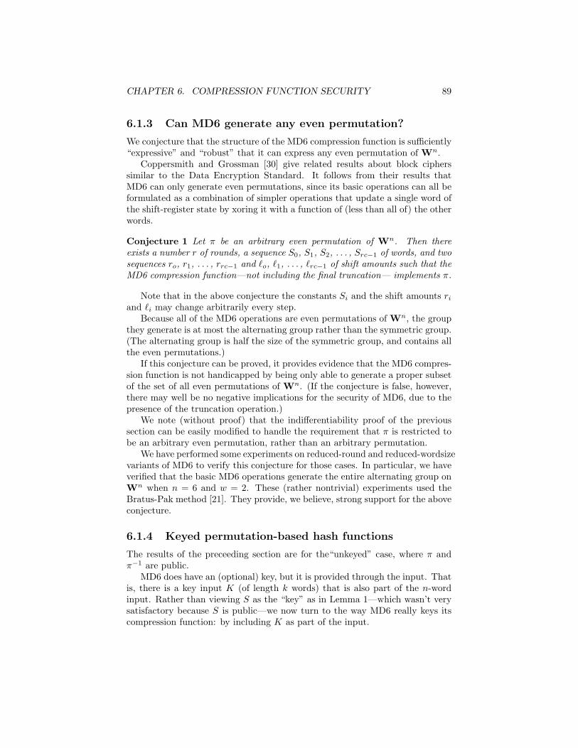
CHAPTER 6. COMPRESSION FUNCTION SECURITY 89
6.1.3 Can MD6 generate any even permutation?
We conjecture that the structure of the MD6 compression function is sufficiently“expressive” and “robust” that it can express any even permutation of Wn.
Coppersmith and Grossman [30] give related results about block cipherssimilar to the Data Encryption Standard. It follows from their results thatMD6 can only generate even permutations, since its basic operations can all beformulated as a combination of simpler operations that update a single word ofthe shift-register state by xoring it with a function of (less than all of) the otherwords.
Conjecture 1 Let π be an arbitrary even permutation of Wn. Then thereexists a number r of rounds, a sequence S0, S1, S2, . . . , Src−1 of words, and twosequences ro, r1, . . . , rrc−1 and `o, `1, . . . , `rc−1 of shift amounts such that theMD6 compression function—not including the final truncation— implements π.
Note that in the above conjecture the constants Si and the shift amounts riand `i may change arbitrarily every step.
Because all of the MD6 operations are even permutations of Wn, the groupthey generate is at most the alternating group rather than the symmetric group.(The alternating group is half the size of the symmetric group, and contains allthe even permutations.)
If this conjecture can be proved, it provides evidence that the MD6 compres-sion function is not handicapped by being only able to generate a proper subsetof the set of all even permutations of Wn. (If the conjecture is false, however,there may well be no negative implications for the security of MD6, due to thepresence of the truncation operation.)
We note (without proof) that the indifferentiability proof of the previoussection can be easily modified to handle the requirement that π is restricted tobe an arbitrary even permutation, rather than an arbitrary permutation.
We have performed some experiments on reduced-round and reduced-wordsizevariants of MD6 to verify this conjecture for those cases. In particular, we haveverified that the basic MD6 operations generate the entire alternating group onWn when n = 6 and w = 2. These (rather nontrivial) experiments used theBratus-Pak method [21]. They provide, we believe, strong support for the aboveconjecture.
6.1.4 Keyed permutation-based hash functions
The results of the preceeding section are for the“unkeyed” case, where π andπ−1 are public.
MD6 does have an (optional) key, but it is provided through the input. Thatis, there is a key input K (of length k words) that is also part of the n-wordinput. Rather than viewing S as the “key” as in Lemma 1—which wasn’t verysatisfactory because S is public—we now turn to the way MD6 really keys itscompression function: by including K as part of the input.
CHAPTER 6. COMPRESSION FUNCTION SECURITY 90
If fQ is indifferentiable from a random oracle, as proven in Theorem 1,then using a portion of its bits for a secret key clearly gives something likea “keyed random oracle”—a family of functions, each indifferentiable from arandom oracle, with one such function for each key. In other words, the MD6compression function is then a pseudorandom function with seed K.
6.1.5 m-bit to n-bit truncation
The NIST requirements state (where n denotes the size of the message digestoutput) in Section 4.A.iii:
Any m-bit hash function specified by taking a fixed subset of thecandidate function’s output bits is expected to meet the above re-quirements with m replacing n. (Note that an attacker can choosethe m-bit subset specifically to allow a limited number of precom-puted message digests to collide, but once the subset has been cho-sen, finding additional violations of the above properties is expectedto be as hard as described above.)
To respond to this requirement, we note that:
• MD6 was designed to follow the principle of “output symmetry” (see Sec-tion 3.11): each output bit is intended to be equivalent to any other outputbit in terms of its effect on security.
• The indifferentiability proof given above suggests that MD6 should notsuffer in any surprising ways if its output is truncated, since the securityof a random oracle does not suffer in any surprising way if its output istruncated.
• MD6 follows the “wide-pipe” strategy suggested by Lucks [54, 55], whereinthe internal chaining variables have at least twice as many bits as thefinal output hash value. The 1024-bit output at the root of the MD6computation tree is truncated to d bits to obtain the final MD6 output.MD6 was designed to be “truncation friendly.”
However, we note that the truncation approach suggested in the NIST pro-posal is at variance with the MD6 design philosophy, since to change the outputdigest size for MD6, one also changes the input to every compression functioncall, in order to avoid the situation where a d-bit hash output and a d′-bit hashoutput are obviously related to each other in a trivial way.
6.2 Choice of compression function constants
6.2.1 Constant Q
The constant Q is chosen rather arbitrarily as the binary representation of thefractional part of
√6. (Why 6? Because it is MD6!)
CHAPTER 6. COMPRESSION FUNCTION SECURITY 91
Other values for Q could have been chosen, even 0. Our proofs do not dependon Q having any particular value; merely that it is fixed.
However, it was felt that a “complex” value such as√
6−2 might have someadvantages over an all-zero value; having many 1-bits in Q would force someAND gates to have non-zero inputs early on. Some of the algebraic attacks doseem to suggest that fewer rounds are needed for security if Q is chosen to benon-zero in a “random-looking” way as MD6 does.
6.2.2 Tap positions
The tap positions were computed by a program, tapopt.c, which is includedwith our MD6 submission to NIST.
The program takes as input the desired values for n and c, and produces asoutput “optimal” values for the tap positions t0, t1, t2, t3, t4, and t5, subjectto the constraints that
•c < t0 < t1 < t2 < t3 < t4 < t5 = n
• The tap positions must all be nonzero modulo c.
• The tap positions must not be equal to each other modulo c.
• The tap positions, other than t5 must be relatively prime to n. (This is atrivial condition if n is prime.)
• The difference t4 − t3 must not be equal to the difference t2 − t1.
The search for an optimal set of tap positions is brute-force; every seqeuenceof possible tap positions satisfying the above constraints is considered.
For a given set of tap positions, the computation of the compression functionis simulated, and for each value A[i] computed, it is recorded which of the inputwords A[0..n − 1 it “formally depends upon.” A word A[i] formally dependsupon input A[j] if i = j or if i > n and at least one of the words A[i− t0], A[i−t1], A[i− t2], A[t3], A[t4], or A[i− t5] formally depends upon A[j].
We can say a word A[i] is “complete” if it formally depends upon all inputwords A[0] . . . A[n− 1].
The “measure” of a set of taps is i − (n − 1) + c, where i is the largest isuch that A[i] is not complete. This value is the least number of steps neededto ensure that all c outputs are formally dependent on all n inputs (and thatrunning more steps won’t change this fact).
The optimization for n = 89, c = 16 takes just a few minutes on a laptop.As discussed and illustrated in Chapter 9, the program tapopt.c can be
used to find optimal tap positions for other choices of n and c.
CHAPTER 6. COMPRESSION FUNCTION SECURITY 92
6.2.3 Shift amounts and properties of g
Once the tap positions were determined, the shift amounts were determined bya second program, shiftopt.c.
Because none of the shift amounts are zero, the function g is one-to-one (i.e.,invertible). Thus, an input change always causes an output change.
Also, as noted in Section 3.9.3, a one-bit change to the input of g will causefrom two to four bits of the output of g to change.
Furthermore, the shift amounts were chosen so that in order to get a one-bitoutput change, at least five bits of input must be changed.
These properties were used in our proof in Section 6.9 of the resistance ofMD6 to differential attacks.
6.2.4 Avalanche properties
The tap positions and the shift amounts were both selected by programs “tapopt”and “shiftopt” in a heuristic but deterministic way that attempts to optimizethe influence of each input bit on each output bit in a minimum number ofsteps.
The tap positions were chosen as described in Section 3.9.1. This “optimiza-tion” only paid attention to word-level dependencies, and ignored bit-position(intraword) effects. It was found that after 102 steps (i.e. just over six rounds)each word computed depends, in a formal sense, on each input word.
After the tap positions were chosen, the shift amounts were chosen deter-ministically from a large pseudorandom sample of shift tables to heuristicallyoptimize the rate of diffusion at the bit-level. The program “shiftopt” ex-plicitly considers the constant and linear terms of the algebraic normal formrepresenting each output bit as a function of the input bits, and measures howclose each such polynomial is to having approximately half of the maximumnumber of possible linear terms present. After a total 11 rounds, the selectedshift amounts heuristically optimized this measure; the output bits appeared“random” based on this metric.
These optimization methods support the hypothesis that the MD6 compres-sion function begins to look “fairly random” after only 11 rounds.
Once the tap positions and shift amounts were selected, other tests, de-scribed in the following sections, help to assess the cryptographic strength ofthe resulting compression function.
6.2.5 Absence of trapdoors
MD6 was designed to be demonstrably free of trapdoors.The architecture of MD6 is remarkably simple; such simplicity makes the
insertion of trapdoors infeasible.Moreover, the various constants of MD6, such as Q =
√6 − 2, the tap
positions, and the shift amounts, are all computed deterministically by programs
CHAPTER 6. COMPRESSION FUNCTION SECURITY 93
that are available for inspection. The computations and optimizations theyimplement are directed towards maximizing the cryptographic strength of MD6.
Thus, while there is of course no guarantee that MD6 is free from crypto-graphic weakness, it is arguably free of maliciously inserted trapdoors.
6.3 Collision resistance
This section studies the security of the MD6 compression function againstcollision-finding attacks. Since a “birthday attack” requires effort only O(2d/2)to find a collision for a hash function with d-bit outputs, the goal here is to findevidence supporting the hypothesis that no attack on MD6 is more efficient, i.e.,that MD6 is collision-resistant.
The theoretical foundations for the MD6 compression function presentedin Section 6.1 support this hypothesis that MD6 is collision-resistant, since abirthday attack is the most efficient collision-finding attack on a random oracle,and MD6 is indifferentiable from a random oracle (under the assumptions ofSection 6.1.2).
There could nonetheless be efficient collision-finding attacks against MD6 —perhaps the underlying assumptions are flawed somehow? It is thus worthwhileto consider known specific collision-finding attacks, to see how well they mightwork. Studies like this also shed light on the question of the number of roundsneeded in MD6.
The two most powerful attacks we know of for finding collisions in a com-pression function are SAT-solver attacks, and differential attacks. Section 6.12presents our results on SAT solver attacks; Section 6.9 presents a major result:that MD6 is resistant to collision-finding based on standard differential attacks.
As we shall see, neither SAT solver attacks nor standard differential attacksare able to find collisions better than the traditional “birthday attacks,” oncethe number of rounds is sufficiently large.
6.4 Preimage Resistance
A good hash function will be preimage-resistant: an adversary will need effortroughly 2d to find any preimage of a d-bit hash.
Again, the theoretical foundations for the MD6 compression function pre-sented in Section 6.1 support the hypothesis that MD6 is preimage-resistant,since a brute-force attack is the most efficient inversion attack on a random or-acle, and MD6 is indifferentiable from a random oracle (under the assumptionsof Section 6.1.2).
Nonetheless, it is worthwhile studying specific attacks that might defeat thepreimage-resistance of MD6. Section 6.12 presents our results on SAT solverattacks. Again, such studies can also help guide the choice of the appropriatenumber of rounds in MD6.
CHAPTER 6. COMPRESSION FUNCTION SECURITY 94
6.5 Second Preimage Resistance
A good hash function will also be second preimage-resistant: an adversary willneed effort O(2d) to find any preimage of a d-bit hash that is different than aninitially given first preimage.
Again, the theoretical foundations for the MD6 compression function pre-sented in Section 6.1 support the hypothesis that MD6 is second preimage-resistant, since a brute-force attack is the most efficient pre-image attack on arandom oracle, and MD6 is indifferentiable from a random oracle (under theassumptions of Section 6.1.2).
Of course, a hash function that is not preimage-resistant is also not secondpreimage resistant. But a hash function may be preimage-resistant but notsecond preimage resistant.
We do not know of any attacks on the second preimage resistance of MD6that are not just attacks on its preimage resistance.
In particular, it is not clear how one might adapt a SAT-solver attack onthe preimage resistance of MD6 to become an attack on the second preimage-resistance of MD6. Our efforts to devise such an adaptation were unsuccessful.
6.6 Pseudorandomness (PRF)
A good (keyed) hash function will appear to be a pseudorandom function (fam-ily). For each key, the hash function will appear to be an independent randomfunction.
The theoretical foundations for the MD6 compression function presentedin Section 6.1 support the hypothesis that MD6 is a pseudorandom functionfamily, since that section argues for the hypothesis that the MD6 compressionfunction is indistinguishable from a random oracle, (under the assumptions givenin Section 6.1.2), and if you declare part of the input of a random oracle to be“key” and the remainder to be “input” (as MD6 does), you end up with apseudorandom function family.
Conversely, any adversary that could distinguish MD6 (as keyed) from apseudorandom function family could be correctly interpreted as an adversaryfor distinguishing the MD6 compression function fQ from a random oracle.
We know of no effective attacks for distinguishing (keyed) MD6 compressionfunction from a pseudorandom function family with the same key, input, andoutput sizes.
The following subsections discuss our attempts to distinguish MD6 from apseudorandom function family by various statistical tests.
6.6.1 Standard statistical tests
A good hash function will pass any standard statistical tests for randomness,such as the NIST Statistical Test Suite. This section reports our efforts to distin-guish the MD6 compression function from a random oracle using two statistical
CHAPTER 6. COMPRESSION FUNCTION SECURITY 95
test suites: the NIST Statistical Test Suite, and TestU01.Both of these statistical test suites are designed to test pseudorandom num-
ber generators. We created a pseudorandom number generator from MD6 byrunning MD6 in counter mode. Let hr,d denote the MD6 hash function pa-rameterized with with digest size d and r rounds. hr,d(m) is the d-bit outputof the parameterized MD6 function on input m. Given a 64-bit seed s, ourPRNG generates the sequence hr,d(s)||hr,d(s + 1)||.... We report the results ofthe chosen statistical tests for d = 512, s = 0 and various choices of r.
These statistical tests fail to detect any nonrandomness in MD6 when MD6has 11 or more rounds.
6.6.1.1 NIST Statistical Test Suite
The NIST Statistical Test Suite is available from http://csrc.nist.gov/groups/ST/toolkit/rng/index.html. The test suite contains implementations of 15different randomness tests.
We ran the NIST statistical tests on MD6 for all r ∈ [0, 35]. For each r, wegenerated 1000 sequences of 1 million bits. Every test from the NIST Test Suitewas run against every bit sequence, generating a list of p-values for every test. Todetermine if a test was successful at distinguishing MD6 from a random numbergenerator, we tested the output p-values for uniformity using a Kolmogorov-Smirnov test. We also compared the actual number of statistically-significantp-values to the expected number. Running the NIST suite for all r ∈ [0, 35]took approximately 10 days.
To our surprise, a few of the NIST tests found MD6 non-random beyond25 rounds. We believe, however, that these tests are incorrectly implemented.We tested this hypothesis by running the NIST tests on SHA-1 (with the fullnumber of rounds), and found that several of the NIST tests also deem SHA-1non-random.
The following table lists the maximum number of rounds of MD6 that eachNIST test is able to distinguish from a random oracle. We have included theresults of the tests we believe to be correctly implemented, i.e. the tests passedby SHA-1.
SHA-1 failed the FFT, OverlappingTemplate, RandomExcursionsVariantand Serial tests, and we have omitted the results for MD6 on these tests. Wereplicated these four tests with the TestU01 suite, however, and found MD6passes these tests for r ≥ 9. The following section describes our experimentswith TestU01 in more detail.
6.6.1.2 TestU01
We also ran MD6 through the TestU01 suite of tests for random number gen-erators. TestU01 was developed by Pierre L’Ecuyer and Richard Simard and isavailable from http://www.iro.umontreal.ca/~simardr/testu01/tu01.html.Further details on TestU01 are available in [53].
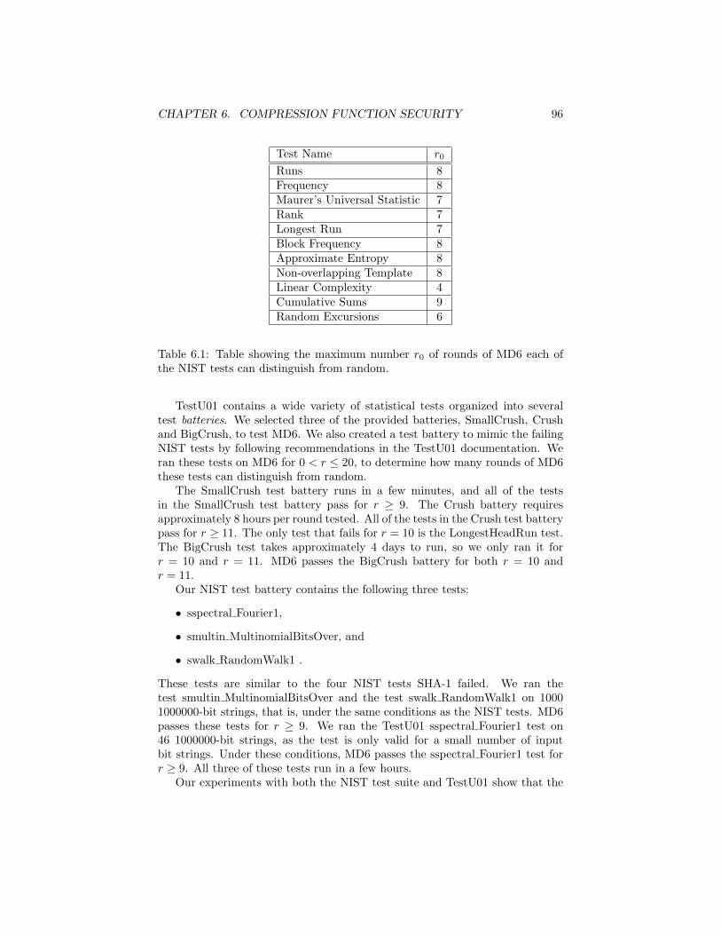
CHAPTER 6. COMPRESSION FUNCTION SECURITY 96
Test Name r0
Runs 8Frequency 8Maurer’s Universal Statistic 7Rank 7Longest Run 7Block Frequency 8Approximate Entropy 8Non-overlapping Template 8Linear Complexity 4Cumulative Sums 9Random Excursions 6
Table 6.1: Table showing the maximum number r0 of rounds of MD6 each ofthe NIST tests can distinguish from random.
TestU01 contains a wide variety of statistical tests organized into severaltest batteries. We selected three of the provided batteries, SmallCrush, Crushand BigCrush, to test MD6. We also created a test battery to mimic the failingNIST tests by following recommendations in the TestU01 documentation. Weran these tests on MD6 for 0 < r ≤ 20, to determine how many rounds of MD6these tests can distinguish from random.
The SmallCrush test battery runs in a few minutes, and all of the testsin the SmallCrush test battery pass for r ≥ 9. The Crush battery requiresapproximately 8 hours per round tested. All of the tests in the Crush test batterypass for r ≥ 11. The only test that fails for r = 10 is the LongestHeadRun test.The BigCrush test takes approximately 4 days to run, so we only ran it forr = 10 and r = 11. MD6 passes the BigCrush battery for both r = 10 andr = 11.
Our NIST test battery contains the following three tests:
• sspectral Fourier1,
• smultin MultinomialBitsOver, and
• swalk RandomWalk1 .
These tests are similar to the four NIST tests SHA-1 failed. We ran thetest smultin MultinomialBitsOver and the test swalk RandomWalk1 on 10001000000-bit strings, that is, under the same conditions as the NIST tests. MD6passes these tests for r ≥ 9. We ran the TestU01 sspectral Fourier1 test on46 1000000-bit strings, as the test is only valid for a small number of inputbit strings. Under these conditions, MD6 passes the sspectral Fourier1 test forr ≥ 9. All three of these tests run in a few hours.
Our experiments with both the NIST test suite and TestU01 show that the
CHAPTER 6. COMPRESSION FUNCTION SECURITY 97
standard statistical tests for pseudorandom number generators cannot distin-guish MD6 from a random oracle when MD6 has 11 or more rounds.
6.6.2 Other statistical tests
This section reports our efforts to distinguish the MD6 compression functionfrom a random oracle using other statistical tests we have devised or adaptedfrom the literature.
We created several influence tests to measure correlations between input andoutput bit positions. Given an input bit position b and an output bit positionc, our tests measure pbc, the probability that flipping bit b causes bit c to flip.For a random oracle, we expect pbc = 1
2 for any choice of b and c.Our tests measure pbc by using the following procedure:
1. Choose an input bit position b, an output bit position c, a number ofrounds r, and a number of trials n.
2. Use RC4 to generate n random 89-word inputs x1, x2, ..., xn to the MD6compression function f .
3. For each input xi, generate a corresponding input x′i by flipping the bthbit of xi.
4. Compare the outputs of the r-round compression function fr(x′i) andfr(xi). Compute the output difference o = fr(x′i)⊕ fr(xi).
5. Count cbc, the number of times o has a 1 in output position c. Computepbc = cbc
n .
For a given input bit b, our influence test simultaneously computes pbc forall output bits c. To test if MD6 behaves significantly differently from a ran-dom oracle, we compared the distribution of the measured pbc values with theexpected distribution from a random oracle. In a random oracle, the pbc valuesare drawn from a binomial distribution with p = 1
2 and n trials. For large n, thisdistribution is essentially normal with mean 1
2 and standard deviation 12√n
. Weused an Anderson-Darling test and a chi-square test to measure the probabilityof our pbc values being drawn from this theoretical distribution.
Table 6.2 reports the results of running the above test on input bit 3648 with1000000 trials. We chose this bit because it is one of the worst-case inputs; it isthe first bit of the 57th input word, which is the last word to be incorporatedinto the hash function computation. Therefore, we expect the influence of bitsin the 57th word to be more detectable than the influence of bits in any otherword.
An Anderson-Darling A∗2 score above 1.035 is significant at the P = 0.01level. Our χ2 test results in a Z-score, for which a score above 2.57 is significantat the P = 0.01 level. These results show that the basic influence test cannotdifferentiate between MD6 and a random oracle beyond 10 rounds. Runningthis test required only a few minutes.
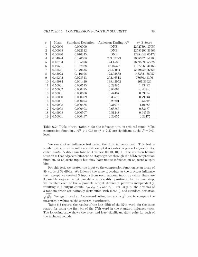
CHAPTER 6. COMPRESSION FUNCTION SECURITY 98
r Mean Standard Deviation Anderson-Darling A∗2 χ2 Z-Score1 0.00000 0.000000 DNE 22627394.370552 0.00098 0.022112 DNE 22583200.319693 0.00880 0.070245 DNE 22284642.004784 0.04094 0.120308 269.07229 20383323.517085 0.10784 0.165396 124.15361 16395698.586226 0.19551 0.187628 42.07427 11577960.411657 0.32541 0.179635 29.50064 5679459.066608 0.43923 0.110198 123.03832 1433321.389579 0.49252 0.028513 262.46513 78630.4130610 0.49984 0.001440 138.43952 167.3902611 0.50001 0.000515 0.29285 1.4349212 0.50002 0.000495 0.84664 -0.4054013 0.50001 0.000506 0.47437 0.5905414 0.50000 0.000509 0.30570 0.7904315 0.50001 0.000494 0.25221 -0.5482816 0.49998 0.000488 0.31075 -1.0178617 0.49998 0.000503 0.63886 0.3317718 0.49998 0.000507 0.51248 0.6459519 0.50001 0.000497 0.22655 -0.29475
Table 6.2: Table of test statistics for the influence test on reduced-round MD6compression functions. A∗2 > 1.035 or χ2 > 2.57 are significant at the P = 0.01level.
We ran another influence test called the dibit influence test. This test issimilar to the previous influence test, except it operates on pairs of adjacent bits,called dibits. A dibit can take on 4 values: 00, 01, 10, 11. The intuition behindthis test is that adjacent bits tend to stay together through the MD6 compressionfunction, so adjacent input bits may have undue influence on adjacent outputbits.
For this test, we treated the input to the compression function as an array of89 words of 32 dibits. We followed the same procedure as the previous influencetest, except we created 3 inputs from each random input xi (since there are3 possible ways an input can differ in one dibit position). In the final step,we counted each of the 4 possible output difference patterns independently,resulting in 4 output counts, c00, c01, c10 and c11. For large n, the c values ofa random oracle are normally distributed with mean n
4 and standard deviation√3
16n . We again used an Anderson-Darling test and a χ2 test to compare themeasured c values to the expected distribution.
Table 6.3 reports the results of the first dibit of the 57th word, for the samereason for using the first bit of the 57th word in the standard influence tests.The following table shows the most and least significant dibit pairs for each ofthe included rounds.
CHAPTER 6. COMPRESSION FUNCTION SECURITY 99
An Anderson-Darling A∗2 score above 1.035 is significant at the P = 0.01level. Our χ2 test results in a Z-score, for which a score above 2.57 is significantat the P = 0.01 level. Our results show that the dibit influence test cannot dif-ferentiate between MD6 and a random oracle beyond approximately 10 rounds.Although there are some statistically significant results for beyond 10 rounds,around 2.4 statistically significant scores are expected since there are a total of240 measurements for each statistic. Running this test took only a few minutes.
Our work with the influence test and its variants shows that these testscannot distinguish MD6 from a random oracle beyond 10 rounds.
6.7 Unpredictability (MAC)
A good (keyed) hash function will also be unpredictable, and thus be usable asa MAC. Unpredictability is implied by pseudorandomness, but is potentially aweaker condition.
We have argued above for the pseudorandomness of the MD6 compressionfunction. We do not have further evidence specific to unpredictability.
6.8 Key-Blinding
In Section 7.6, we set out to prove that the overall MD6 hash function hasthe property of unpredictability, assuming that the compression function usedalso has this property. Unfortunately, we were not able to provide such a proofwith only that base assumption; however, if we make an additional non-trivialassumption about the compression function we are able to prove the unpre-dictability of MD6.
The idea for the following is that the flag bit z which indicates that thecompression function application is the final one in the computation of MD6should “blind” the key values. That is, if we are given oracle access to twofunctions defined as follows
f0Q(·) = fQ(z = 0,K = κ0, ·)f1Q(·) = fQ(z = 1,K = κ1, ·)
then we should not be able to guess whether κ0 and κ1 are equivalent or notwith any significant advantage. The intuition behind this assumption is that weneed fQ to behave in a “pseudorandom” fashion, but only on the z bit of theinput.
Definition 2 (Key-Blinding Assumption) Let D be a distinguisher givenoracle access to two functions f0
Q and f1Q that map Wk ×Wn−q−k−1 → Wc.
We define its advantage as follows.
AdvblindD,fQ
(t, q) =
∣∣∣∣∣ Pr
[κ0
$←Wk;κ1$←Wk; b $← {0, 1};
a← DfQ(z=0,κ0,·),fQ(z=1,κb,·): a = b
]− 1
2
∣∣∣∣∣
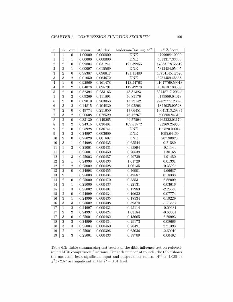
CHAPTER 6. COMPRESSION FUNCTION SECURITY 100
r in out mean std dev Anderson-Darling A∗2 χ2 Z-Score1 1 0 1.00000 0.000000 DNE 47999984.00001 1 1 0.00000 0.000000 DNE 5333317.333332 2 0 0.99804 0.031241 197.39955 47833178.565192 3 1 0.00097 0.015569 DNE 5312484.054953 2 0 0.98387 0.096617 181.11400 46754145.475203 3 2 0.01050 0.064672 DNE 5251459.456384 1 0 0.92969 0.161478 113.54763 41647769.599134 3 2 0.04078 0.095791 112.42278 4518137.305095 2 0 0.82394 0.233163 48.31323 32748717.205455 3 2 0.09269 0.111891 46.85176 3179889.040786 2 0 0.69010 0.263053 13.72142 22432777.235966 3 2 0.14815 0.104830 26.92808 1822935.905287 2 0 0.49774 0.251650 17.06451 10641313.298847 3 2 0.20608 0.078529 46.12267 690808.843108 2 0 0.33130 0.149265 69.57594 2465222.031798 3 2 0.24315 0.030481 109.51572 83269.259369 2 0 0.25928 0.036741 DNE 122520.000149 3 2 0.24997 0.003609 DNE 1095.6446910 2 0 0.25020 0.001607 DNE 207.9082810 3 1 0.24998 0.000435 0.65544 0.2158911 1 2 0.25001 0.000431 0.33894 -0.1303911 3 1 0.25001 0.000450 0.20539 1.3016812 1 3 0.25003 0.000457 0.29739 1.9145012 2 1 0.24998 0.000433 1.01729 0.0133112 2 2 0.25002 0.000428 1.06135 -0.3390513 2 0 0.24998 0.000455 0.76901 1.6668713 2 1 0.25003 0.000434 0.42587 0.1833314 2 0 0.25000 0.000470 0.58531 2.8800914 3 1 0.25000 0.000433 0.22131 0.0361615 1 3 0.25002 0.000401 0.17983 -2.2664015 2 0 0.24999 0.000434 0.19632 0.0777416 3 1 0.24999 0.000435 0.18534 0.1922916 3 3 0.25002 0.000408 0.39370 -1.7355717 1 2 0.24997 0.000431 0.25114 -0.0963117 2 2 0.24997 0.000424 1.03184 -0.6305417 3 0 0.25001 0.000462 0.13665 2.2099318 2 3 0.24999 0.000434 0.29173 0.0866618 3 3 0.25004 0.000460 0.26491 2.2139319 2 1 0.25001 0.000396 0.65036 -2.6001019 2 3 0.25001 0.000433 0.39709 0.00462
Table 6.3: Table summarizing test results of the dibit influence test on reduced-round MD6 compression functions. For each number of rounds, the table showsthe most and least significant input and output dibit values. A∗2 > 1.035 orχ2 > 2.57 are significant at the P = 0.01 level.
CHAPTER 6. COMPRESSION FUNCTION SECURITY 101
The goal of D is to try to determine the value of b, i.e. whether f0Q and f1
Q usethe same key or not. We can define the overall insecurity of the key-blindingproperty of fQ to be
InSecblindfQ
(t, q) = maxD
{Advblind
D,fQ(t, q)
},
where D is given resource constraints of (t, q).
Given our work above supporting the proposition that MD6 is a pseudoran-dom function, the restriction of this proposition to the weaker proposition thatMD6 satisfies the key-blinding assumption appears quite reasonable.
6.9 Differential cryptanalysis
Differential cryptanalysis was pioneered by Biham and Shamir [15] in the early90s, and it was the first type of sophisicated analytical attacks on block ciphersincluding the Data Encryption Standard. Subsequently, Preneel et al. [81] pro-posed the differential cryptanalysis of hash functions based on block ciphers.
Differential attacks have in fact been surprisingly successful and effectiveagainst a number of hash functions. MD4, RIPEMD, and 3-pass HAVAL [94,98], MD5 [96], SHA-0 [27, 16, 17, 97] and SHA-1 [17, 95] have all fallen. ProfessorXiaoyun Wang has led these attacks.
In this section, we analyze the security of MD6 with respect to differentialcryptanalysis. As in most security analysis, our goal is two-fold—we hope toprovide both “attacks (upper bounds)” and “lower bounds”. Our major resultis a lower bound showing that there is no standard differential attack againstMD6 that is more effective than a naive “birthday” attack.
The rest of the section is organized as follows. In Section 6.9.1, we describesome useful definitions in differential cryptanalysis. In Section 6.9.2 we ana-lyze differential properties of the MD6 step function by analyzing individualoperations. Throughout our discussions, we will pay special attention to defi-nitions and properties that are important in the later lower bound analysis. InSection 6.9.3, we prove a lower bound on the workload of any differential-stylecollision attacks. Finally, in Section 6.9.4, we present some preliminary resultsrelated to upper bound analysis.
6.9.1 Basic definitions and assumptions
Differential cryptanalysis of block ciphers falls into the category of chosen plain-text attacks. The basic idea is that two plaintexts with a carefully chosen dif-ference can encipher to two ciphertexts such that their difference has a specificvalue with non-negligible probability, and by taking sufficiently many plain-text/ciphertext pairs and analyzing their differences, certain bits of the secretkey may be revealed.
In the context of a (keyless) hash function, the goal of differential cryptanal-ysis is to find message pairs with an appropriately chosen difference such that
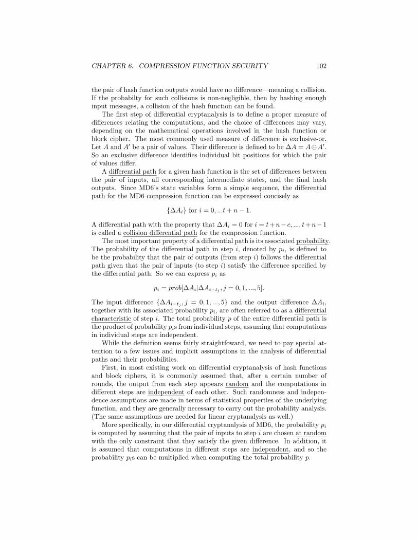
CHAPTER 6. COMPRESSION FUNCTION SECURITY 102
the pair of hash function outputs would have no difference—meaning a collision.If the probabilty for such collisions is non-negligible, then by hashing enoughinput messages, a collision of the hash function can be found.
The first step of differential cryptanalysis is to define a proper measure ofdifferences relating the computations, and the choice of differences may vary,depending on the mathematical operations involved in the hash function orblock cipher. The most commonly used measure of difference is exclusive-or.Let A and A′ be a pair of values. Their difference is defined to be ∆A = A⊕A′.So an exclusive difference identifies individual bit positions for which the pairof values differ.
A differential path for a given hash function is the set of differences betweenthe pair of inputs, all corresponding intermediate states, and the final hashoutputs. Since MD6’s state variables form a simple sequence, the differentialpath for the MD6 compression function can be expressed concisely as
{∆Ai} for i = 0, ...t+ n− 1.
A differential path with the property that ∆Ai = 0 for i = t+n− c, ..., t+n−1is called a collision differential path for the compression function.
The most important property of a differential path is its associated probability.The probability of the differential path in step i, denoted by pi, is defined tobe the probability that the pair of outputs (from step i) follows the differentialpath given that the pair of inputs (to step i) satisfy the difference specified bythe differential path. So we can express pi as
pi = prob[∆Ai|∆Ai−tj , j = 0, 1, ..., 5].
The input difference {∆Ai−tj , j = 0, 1, ..., 5} and the output difference ∆Ai,together with its associated probability pi, are often referred to as a differentialcharacteristic of step i. The total probability p of the entire differential path isthe product of probability pis from individual steps, assuming that computationsin individual steps are independent.
While the definition seems fairly straightfoward, we need to pay special at-tention to a few issues and implicit assumptions in the analysis of differentialpaths and their probabilities.
First, in most existing work on differential cryptanalysis of hash functionsand block ciphers, it is commonly assumed that, after a certain number ofrounds, the output from each step appears random and the computations indifferent steps are independent of each other. Such randomness and indepen-dence assumptions are made in terms of statistical properties of the underlyingfunction, and they are generally necessary to carry out the probability analysis.(The same assumptions are needed for linear cryptanalysis as well.)
More specifically, in our differential cryptanalysis of MD6, the probability piis computed by assuming that the pair of inputs to step i are chosen at randomwith the only constraint that they satisfy the given difference. In addition, itis assumed that computations in different steps are independent, and so theprobability pis can be multiplied when computing the total probability p.
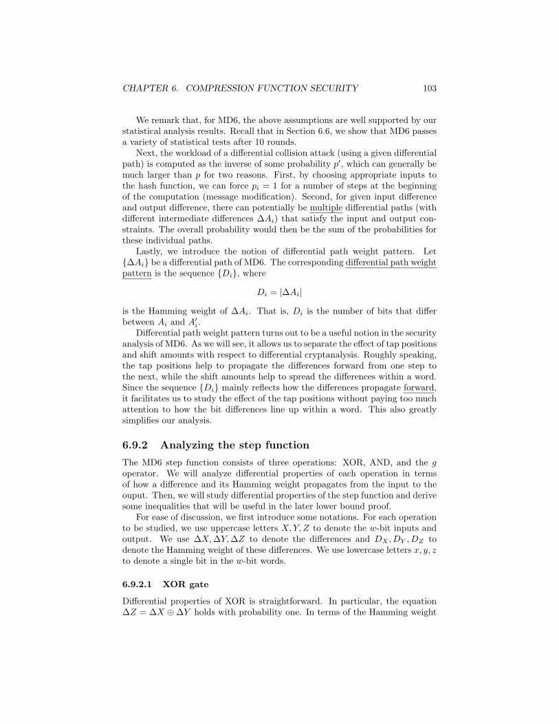
CHAPTER 6. COMPRESSION FUNCTION SECURITY 103
We remark that, for MD6, the above assumptions are well supported by ourstatistical analysis results. Recall that in Section 6.6, we show that MD6 passesa variety of statistical tests after 10 rounds.
Next, the workload of a differential collision attack (using a given differentialpath) is computed as the inverse of some probability p′, which can generally bemuch larger than p for two reasons. First, by choosing appropriate inputs tothe hash function, we can force pi = 1 for a number of steps at the beginningof the computation (message modification). Second, for given input differenceand output difference, there can potentially be multiple differential paths (withdifferent intermediate differences ∆Ai) that satisfy the input and output con-straints. The overall probability would then be the sum of the probabilities forthese individual paths.
Lastly, we introduce the notion of differential path weight pattern. Let{∆Ai} be a differential path of MD6. The corresponding differential path weightpattern is the sequence {Di}, where
Di = |∆Ai|
is the Hamming weight of ∆Ai. That is, Di is the number of bits that differbetween Ai and A′i.
Differential path weight pattern turns out to be a useful notion in the securityanalysis of MD6. As we will see, it allows us to separate the effect of tap positionsand shift amounts with respect to differential cryptanalysis. Roughly speaking,the tap positions help to propagate the differences forward from one step tothe next, while the shift amounts help to spread the differences within a word.Since the sequence {Di} mainly reflects how the differences propagate forward,it facilitates us to study the effect of the tap positions without paying too muchattention to how the bit differences line up within a word. This also greatlysimplifies our analysis.
6.9.2 Analyzing the step function
The MD6 step function consists of three operations: XOR, AND, and the goperator. We will analyze differential properties of each operation in termsof how a difference and its Hamming weight propagates from the input to theouput. Then, we will study differential properties of the step function and derivesome inequalities that will be useful in the later lower bound proof.
For ease of discussion, we first introduce some notations. For each operationto be studied, we use uppercase letters X,Y, Z to denote the w-bit inputs andoutput. We use ∆X,∆Y,∆Z to denote the differences and DX , DY , DZ todenote the Hamming weight of these differences. We use lowercase letters x, y, zto denote a single bit in the w-bit words.
6.9.2.1 XOR gate
Differential properties of XOR is straightforward. In particular, the equation∆Z = ∆X ⊕∆Y holds with probability one. In terms of the Hamming weight
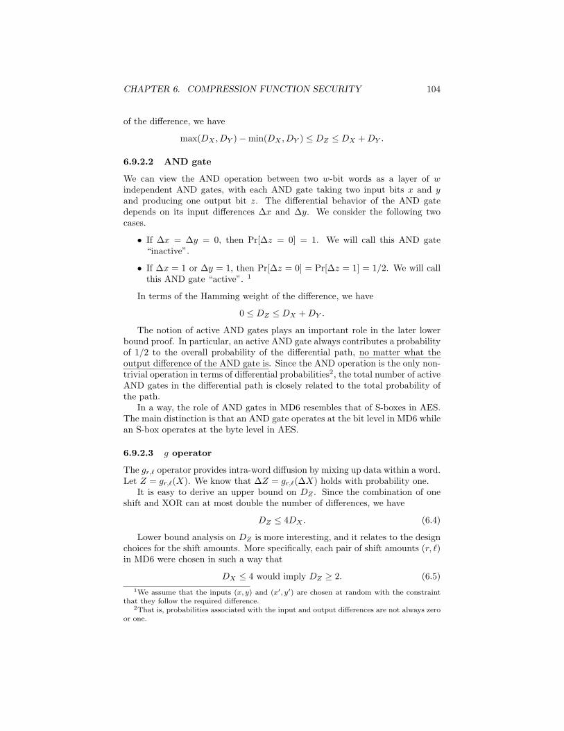
CHAPTER 6. COMPRESSION FUNCTION SECURITY 104
of the difference, we have
max(DX , DY )−min(DX , DY ) ≤ DZ ≤ DX +DY .
6.9.2.2 AND gate
We can view the AND operation between two w-bit words as a layer of windependent AND gates, with each AND gate taking two input bits x and yand producing one output bit z. The differential behavior of the AND gatedepends on its input differences ∆x and ∆y. We consider the following twocases.
• If ∆x = ∆y = 0, then Pr[∆z = 0] = 1. We will call this AND gate“inactive”.
• If ∆x = 1 or ∆y = 1, then Pr[∆z = 0] = Pr[∆z = 1] = 1/2. We will callthis AND gate “active”. 1
In terms of the Hamming weight of the difference, we have
0 ≤ DZ ≤ DX +DY .
The notion of active AND gates plays an important role in the later lowerbound proof. In particular, an active AND gate always contributes a probabilityof 1/2 to the overall probability of the differential path, no matter what theoutput difference of the AND gate is. Since the AND operation is the only non-trivial operation in terms of differential probabilities2, the total number of activeAND gates in the differential path is closely related to the total probability ofthe path.
In a way, the role of AND gates in MD6 resembles that of S-boxes in AES.The main distinction is that an AND gate operates at the bit level in MD6 whilean S-box operates at the byte level in AES.
6.9.2.3 g operator
The gr,` operator provides intra-word diffusion by mixing up data within a word.Let Z = gr,`(X). We know that ∆Z = gr,`(∆X) holds with probability one.
It is easy to derive an upper bound on DZ . Since the combination of oneshift and XOR can at most double the number of differences, we have
DZ ≤ 4DX . (6.4)
Lower bound analysis on DZ is more interesting, and it relates to the designchoices for the shift amounts. More specifically, each pair of shift amounts (r, `)in MD6 were chosen in such a way that
DX ≤ 4 would imply DZ ≥ 2. (6.5)1We assume that the inputs (x, y) and (x′, y′) are chosen at random with the constraint
that they follow the required difference.2That is, probabilities associated with the input and output differences are not always zero
or one.
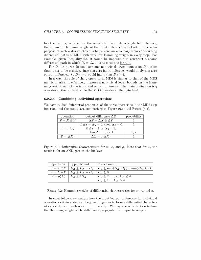
CHAPTER 6. COMPRESSION FUNCTION SECURITY 105
In other words, in order for the output to have only a single bit difference,the minimum Hamming weight of the input difference is at least 5. The mainpurpose of such a design choice is to prevent an adversary from constructingdifferential paths of MD6 with very low Hamming weight in every step. Forexample, given Inequality 6.5, it would be impossible to construct a sparsedifferential path in which Di = |∆Ai| is at most one for all i.
For DX > 4, we do not have any non-trivial lower bounds on DZ otherthan it has to be positive, since non-zero input difference would imply non-zerooutput difference. So DX > 4 would imply that DZ ≥ 1.
In a way, the role of the g operator in MD6 is similar to that of the MDSmatrix in AES. It effectively imposes a non-trivial lower bounds on the Ham-ming weight sum of the input and output difference. The main distinction is goperates at the bit level while the MDS operates at the byte level.
6.9.2.4 Combining individual operations
We have studied differential properties of the three operations in the MD6 stepfunction, and the results are summarized in Figure (6.1) and Figure (6.2).
operation output difference ∆Z probabilityZ = X ⊕ Y ∆Z = ∆X ⊕∆Y 1
if ∆x = ∆y = 0, then ∆z = 0 1z = x ∧ y if ∆x = 1 or ∆y = 1,
then ∆z = 0 or 1 1/2Z = g(X) ∆Z = g(∆X) 1
Figure 6.1: Differential characteristics for ⊕, ∧, and g. Note that for ∧, theresult is for an AND gate at the bit level.
operation upper bound lower boundZ = X ⊕ Y DZ ≤ DX +DY DZ ≥ max(DX , DY )−min(DX , DY )Z = X ∧ Y DZ ≤ DX +DY DZ ≥ 0Z = g(X) DZ ≤ 4DX DZ ≥ 2, if 0 < DX ≤ 4
DZ ≥ 1, if DX > 4
Figure 6.2: Hamming weight of differential characteristics for ⊕, ∧, and g.
In what follows, we analyze how the input/output differences for individualoperations within a step can be joined together to form a differential character-istics for the step with non-zero probability. We pay special attention to howthe Hamming weight of the differences propagate from input to output.
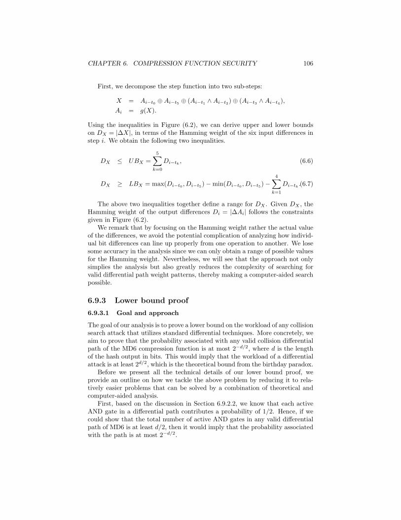
CHAPTER 6. COMPRESSION FUNCTION SECURITY 106
First, we decompose the step function into two sub-steps:
X = Ai−t0 ⊕Ai−t5 ⊕ (Ai−t1 ∧Ai−t2)⊕ (Ai−t3 ∧Ai−t4),Ai = g(X).
Using the inequalities in Figure (6.2), we can derive upper and lower boundson DX = |∆X|, in terms of the Hamming weight of the six input differences instep i. We obtain the following two inequalities.
DX ≤ UBX =5∑k=0
Di−tk , (6.6)
DX ≥ LBX = max(Di−t0 , Di−t5)−min(Di−t0 , Di−t5)−4∑k=1
Di−tk .(6.7)
The above two inequalities together define a range for DX . Given DX , theHamming weight of the output differences Di = |∆Ai| follows the constraintsgiven in Figure (6.2).
We remark that by focusing on the Hamming weight rather the actual valueof the differences, we avoid the potential complication of analyzing how individ-ual bit differences can line up properly from one operation to another. We losesome accuracy in the analysis since we can only obtain a range of possible valuesfor the Hamming weight. Nevertheless, we will see that the approach not onlysimplies the analysis but also greatly reduces the complexity of searching forvalid differential path weight patterns, thereby making a computer-aided searchpossible.
6.9.3 Lower bound proof
6.9.3.1 Goal and approach
The goal of our analysis is to prove a lower bound on the workload of any collisionsearch attack that utilizes standard differential techniques. More concretely, weaim to prove that the probability associated with any valid collision differentialpath of the MD6 compression function is at most 2−d/2, where d is the lengthof the hash output in bits. This would imply that the workload of a differentialattack is at least 2d/2, which is the theoretical bound from the birthday paradox.
Before we present all the technical details of our lower bound proof, weprovide an outline on how we tackle the above problem by reducing it to rela-tively easier problems that can be solved by a combination of theoretical andcomputer-aided analysis.
First, based on the discussion in Section 6.9.2.2, we know that each activeAND gate in a differential path contributes a probability of 1/2. Hence, if wecould show that the total number of active AND gates in any valid differentialpath of MD6 is at least d/2, then it would imply that the probability associatedwith the path is at most 2−d/2.
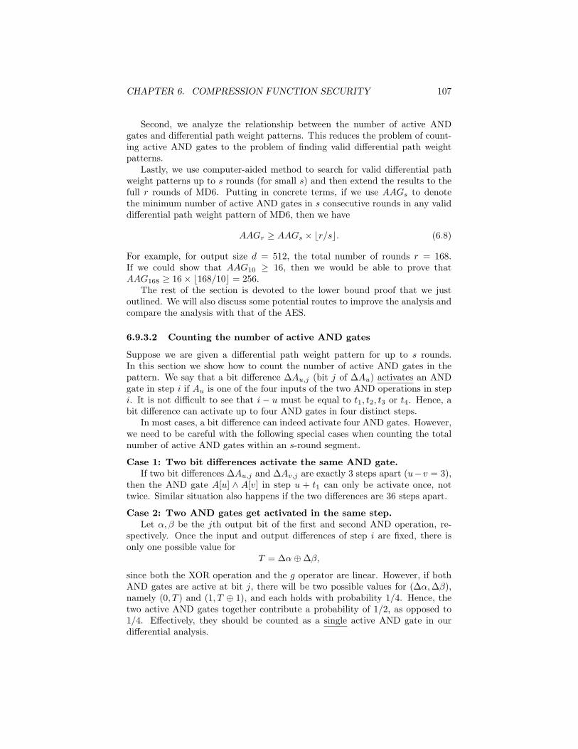
CHAPTER 6. COMPRESSION FUNCTION SECURITY 107
Second, we analyze the relationship between the number of active ANDgates and differential path weight patterns. This reduces the problem of count-ing active AND gates to the problem of finding valid differential path weightpatterns.
Lastly, we use computer-aided method to search for valid differential pathweight patterns up to s rounds (for small s) and then extend the results to thefull r rounds of MD6. Putting in concrete terms, if we use AAGs to denotethe minimum number of active AND gates in s consecutive rounds in any validdifferential path weight pattern of MD6, then we have
AAGr ≥ AAGs × br/sc. (6.8)
For example, for output size d = 512, the total number of rounds r = 168.If we could show that AAG10 ≥ 16, then we would be able to prove thatAAG168 ≥ 16× b168/10c = 256.
The rest of the section is devoted to the lower bound proof that we justoutlined. We will also discuss some potential routes to improve the analysis andcompare the analysis with that of the AES.
6.9.3.2 Counting the number of active AND gates
Suppose we are given a differential path weight pattern for up to s rounds.In this section we show how to count the number of active AND gates in thepattern. We say that a bit difference ∆Au,j (bit j of ∆Au) activates an ANDgate in step i if Au is one of the four inputs of the two AND operations in stepi. It is not difficult to see that i − u must be equal to t1, t2, t3 or t4. Hence, abit difference can activate up to four AND gates in four distinct steps.
In most cases, a bit difference can indeed activate four AND gates. However,we need to be careful with the following special cases when counting the totalnumber of active AND gates within an s-round segment.
Case 1: Two bit differences activate the same AND gate.If two bit differences ∆Au,j and ∆Av,j are exactly 3 steps apart (u−v = 3),
then the AND gate A[u] ∧ A[v] in step u + t1 can only be activate once, nottwice. Similar situation also happens if the two differences are 36 steps apart.
Case 2: Two AND gates get activated in the same step.Let α, β be the jth output bit of the first and second AND operation, re-
spectively. Once the input and output differences of step i are fixed, there isonly one possible value for
T = ∆α⊕∆β,
since both the XOR operation and the g operator are linear. However, if bothAND gates are active at bit j, there will be two possible values for (∆α,∆β),namely (0, T ) and (1, T ⊕ 1), and each holds with probability 1/4. Hence, thetwo active AND gates together contribute a probability of 1/2, as opposed to1/4. Effectively, they should be counted as a single active AND gate in ourdifferential analysis.
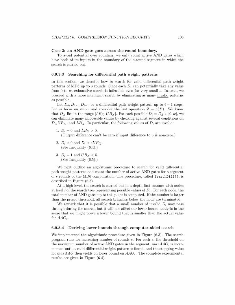
CHAPTER 6. COMPRESSION FUNCTION SECURITY 108
Case 3: an AND gate goes across the round boundary.To avoid potential over counting, we only count active AND gates which
have both of its inputs in the boundary of the s-round segment in which thesearch is carried out.
6.9.3.3 Searching for differential path weight patterns
In this section, we describe how to search for valid differential path weightpatterns of MD6 up to s rounds. Since each Di can potentially take any valuefrom 0 to w, exhaustive search is infeasible even for very small s. Instead, weproceed with a more intelligent search by eliminating as many invalid patternsas possible.
Let D0, D1, ...Di−1 be a differential path weight pattern up to i − 1 steps.Let us focus on step i and consider the last operation Z = g(X). We knowthat DX lies in the range [LBX , UBX ]. For each possible Di = DZ ∈ [0, w], wecan eliminate many impossible values by checking against several conditions onDi, UBX , and LBX . In particular, the following values of Di are invalid:
1. Di = 0 and LBX > 0.(Output difference can’t be zero if input difference to g is non-zero.)
2. Di > 0 and Di > 4UBX .(See Inequality (6.4).)
3. Di = 1 and UBX < 5.(See Inequality (6.5).)
We next outline an algorithmic procedure to search for valid differentialpath weight patterns and count the number of active AND gates for a segmentof s rounds of the MD6 computation. The procedure, called SearchDiff(), isdescribed in Figure (6.3).
At a high level, the search is carried out in a depth-first manner with nodesat level i of the search tree representing possible values of Di. For each node, thetotal number of AND gates up to this point is computed. If the number is largerthan the preset threshold, all search branches below the node are terminated.
We remark that it is possible that a small number of invalid Di may passthrough during the search, but it will not affect our lower bound analysis in thesense that we might prove a lower bound that is smaller than the actual valuefor AAGs.
6.9.3.4 Deriving lower bounds through computer-aided search
We implemented the algorithmic procedure given in Figure (6.3). The searchprogram runs for increasing number of rounds s. For each s, the threshold onthe maximum number of active AND gates in the segment, maxAAG, is incre-mented until a valid differential weight pattern is found, and the stopping valuefor maxAAG then yields on lower bound on AAGs. The complete experimentalresults are given in Figure (6.4).
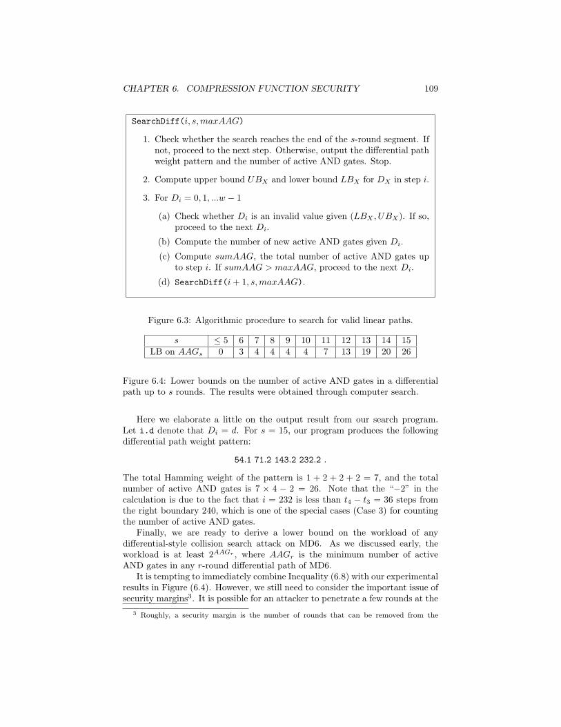
CHAPTER 6. COMPRESSION FUNCTION SECURITY 109
SearchDiff(i, s,maxAAG)
1. Check whether the search reaches the end of the s-round segment. Ifnot, proceed to the next step. Otherwise, output the differential pathweight pattern and the number of active AND gates. Stop.
2. Compute upper bound UBX and lower bound LBX for DX in step i.
3. For Di = 0, 1, ...w − 1
(a) Check whether Di is an invalid value given (LBX , UBX). If so,proceed to the next Di.
(b) Compute the number of new active AND gates given Di.
(c) Compute sumAAG, the total number of active AND gates upto step i. If sumAAG > maxAAG, proceed to the next Di.
(d) SearchDiff(i+ 1, s,maxAAG).
Figure 6.3: Algorithmic procedure to search for valid linear paths.
s ≤ 5 6 7 8 9 10 11 12 13 14 15LB on AAGs 0 3 4 4 4 4 7 13 19 20 26
Figure 6.4: Lower bounds on the number of active AND gates in a differentialpath up to s rounds. The results were obtained through computer search.
Here we elaborate a little on the output result from our search program.Let i.d denote that Di = d. For s = 15, our program produces the followingdifferential path weight pattern:
54.1 71.2 143.2 232.2 .
The total Hamming weight of the pattern is 1 + 2 + 2 + 2 = 7, and the totalnumber of active AND gates is 7 × 4 − 2 = 26. Note that the “−2” in thecalculation is due to the fact that i = 232 is less than t4 − t3 = 36 steps fromthe right boundary 240, which is one of the special cases (Case 3) for countingthe number of active AND gates.
Finally, we are ready to derive a lower bound on the workload of anydifferential-style collision search attack on MD6. As we discussed early, theworkload is at least 2AAGr , where AAGr is the minimum number of activeAND gates in any r-round differential path of MD6.
It is tempting to immediately combine Inequality (6.8) with our experimentalresults in Figure (6.4). However, we still need to consider the important issue ofsecurity margins3. It is possible for an attacker to penetrate a few rounds at the
3 Roughly, a security margin is the number of rounds that can be removed from the
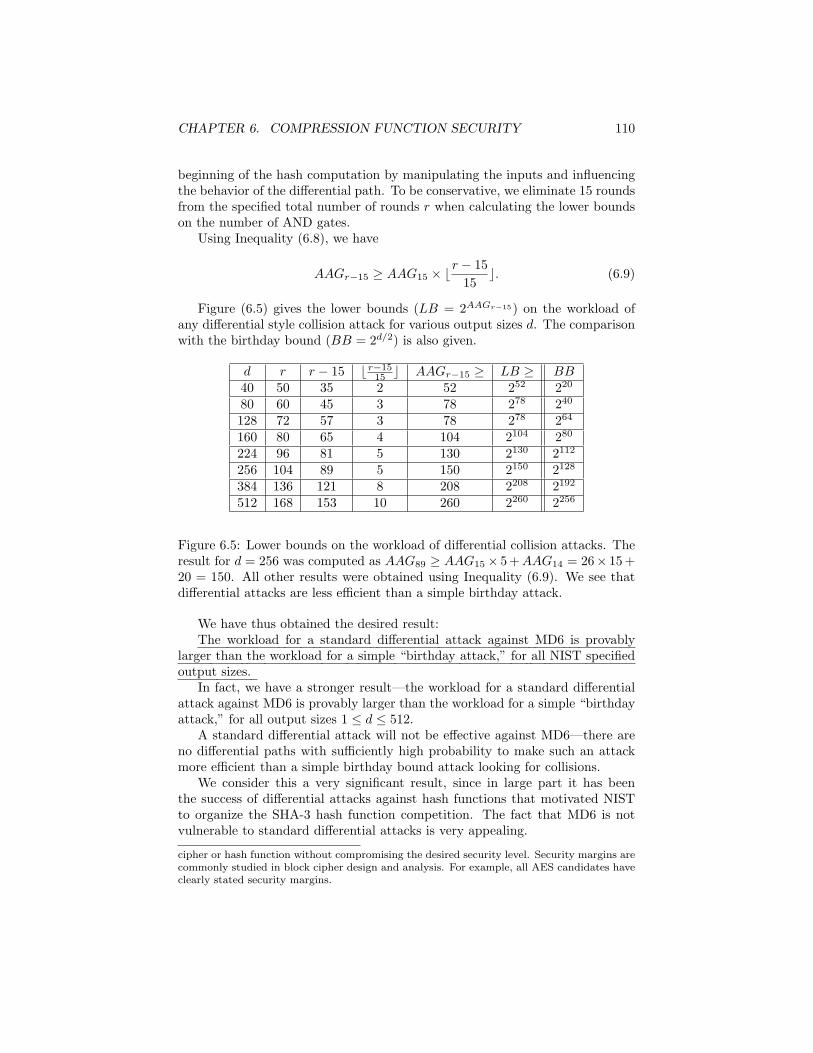
CHAPTER 6. COMPRESSION FUNCTION SECURITY 110
beginning of the hash computation by manipulating the inputs and influencingthe behavior of the differential path. To be conservative, we eliminate 15 roundsfrom the specified total number of rounds r when calculating the lower boundson the number of AND gates.
Using Inequality (6.8), we have
AAGr−15 ≥ AAG15 × br − 15
15c. (6.9)
Figure (6.5) gives the lower bounds (LB = 2AAGr−15) on the workload ofany differential style collision attack for various output sizes d. The comparisonwith the birthday bound (BB = 2d/2) is also given.
d r r − 15 b r−1515 c AAGr−15 ≥ LB ≥ BB
40 50 35 2 52 252 220
80 60 45 3 78 278 240
128 72 57 3 78 278 264
160 80 65 4 104 2104 280
224 96 81 5 130 2130 2112
256 104 89 5 150 2150 2128
384 136 121 8 208 2208 2192
512 168 153 10 260 2260 2256
Figure 6.5: Lower bounds on the workload of differential collision attacks. Theresult for d = 256 was computed as AAG89 ≥ AAG15× 5 +AAG14 = 26× 15 +20 = 150. All other results were obtained using Inequality (6.9). We see thatdifferential attacks are less efficient than a simple birthday attack.
We have thus obtained the desired result:The workload for a standard differential attack against MD6 is provably
larger than the workload for a simple “birthday attack,” for all NIST specifiedoutput sizes.
In fact, we have a stronger result—the workload for a standard differentialattack against MD6 is provably larger than the workload for a simple “birthdayattack,” for all output sizes 1 ≤ d ≤ 512.
A standard differential attack will not be effective against MD6—there areno differential paths with sufficiently high probability to make such an attackmore efficient than a simple birthday bound attack looking for collisions.
We consider this a very significant result, since in large part it has beenthe success of differential attacks against hash functions that motivated NISTto organize the SHA-3 hash function competition. The fact that MD6 is notvulnerable to standard differential attacks is very appealing.
cipher or hash function without compromising the desired security level. Security margins arecommonly studied in block cipher design and analysis. For example, all AES candidates haveclearly stated security margins.
CHAPTER 6. COMPRESSION FUNCTION SECURITY 111
Of course, there may be nonstandard differential attacks (e.g. that usedvarious forms of generalized differentials, as in [25]) that fall outside the scopeof our proof. Further research is needed to explore and exclude such possibilities;our proof is merely a first step in such analysis.
On the other hand, there is probably a significant amount of “slack” in ourresult, and thus the bound could be made tighter and/or extended to moregeneral attacks. It is quite possible that the actual lower bound on the numberof active AND gates can be much larger. Here we list some of the reasons:
• Some of the differential path weight patterns may not correspond to anyvalid differential path of MD6.
• The s-round differential path weight pattern that our program found isnot iterative, and so it cannot be concatenated to yield a pattern for rrounds.
• We did not count the AND gates across the boundary of two consecutiverounds.
If we can address some of the above problems, then we can further improveour lower bound analysis. It would also be interesting to explore how thesebounds might be affected by other choices for the tap positions.
6.9.3.5 Related work
The use of computer-aided search in our lower bound proof was motivated bythe work of Julta and Patthak. In [48], they showed how to derive lower boundson collision probabilities of SHA-1 using computer-aided proof.
Here we briefly describe the key idea in their proof. In SHA-1, the inputmessage, represented by a 16-by-32 0-1 matrix, is expanded to an 80-by-32matrix W . Based on earlier differential cryptanalysis of SHA (e.g. [27]), each setbit in W contributes a probability q (q averaging 2−2.5) to the overall probabilityof the differential collision path. Hence, a lower bound on the number of 1’s in Wwill yield an upper bound on the collision probability. The proof in [48] proceedsby first identifying possible configurations of W and then using computer-aidedsearch to find lower bounds on the number of 1’s for some of the configurations.
The high-level reasoning in our lower bound proof is in a way similar to thatof the AES [33]. Roughly, the proof arguments for AES being secure againststandard differential attacks are as follows:
• Each active S-box in AES has a differential probability of at most 2−5.
• In four consecutive rounds of AES, there are at least 25 active S-boxes ifthe plaintext difference is non-zero4.
• So the probability of any four-round differential path is at most 2−150.4This is due to the following differential property of the MDS matrix: the sum of the
number of non-zero input bytes and non-zero output bytes is at least 5.
CHAPTER 6. COMPRESSION FUNCTION SECURITY 112
As we noted earlier, active AND gates in MD6 correspond to active S-boxesin AES. In addition, the effect of the g operator in MD6 is similar to that ofthe MDS matrix in AES. Therefore it is not a coincidence that the proofs ofsecurity bear some similarities.
6.9.4 Preliminary results related to upper bounds
Our research on finding a lower bound on the complexity of standard differentialattacks worked by exploring the various possibilities an adversary might try toactually find a standard differential attack. However, it organized this explo-ration by looking at differential path weight patterns rather than differentialpaths, and derived a lower bound by looking at 15-round segments rather thana complete MD6 computation.
An interesting question is whether we can derive any differential attack witha complexity that is anywhere near our lower bound. So far we have beenunsuccessful.
To begin with, one would need to find a differential weight pattern thatspanned an entire MD6 computation. Following common approaches in differ-ential cryptanalysis of block ciphers, we try to find iterative differential pathweight patterns for MD6, since an iterative pattern allows one to construct adifferential path weight pattern for as many rounds as possible.
By modifying our search program for the lower bound proof, we are able tofind some interesting iterative differential path weight patterns for MD6. Oneof the iterative differential path weight pattern for 5 rotation is described below.
0.2 89.2 106.2 123.2 140.2156.2 157.2 178.2 212.2 229.2267.2 284.2 301.2 356.2 373.2445.2 534.2 551.2 ...
In the above iterative differential weight pattern, the pattern starts to repeatat step 445, since 534 − 445 = 89 − 2 = 89. The total number of differencesis 30 in the segment of 445 steps, and the number of active AND gates is30× 4− 2 = 118.
It is worth comparing this upper bound result with our lower bound re-sult in terms of avgAAG, the average number of active AND gates per round.First, since 118/(445/16) ≈ 4.24, the iterative pattern for 445 steps implies thatavgAAG ≤ 4.24. Next, our earlier lower bound on AAG15 (see Figure (6.4))implies that avgAAG ≥ 26/15 ≈ 1.73. So there is a gap between the upper andlower bound. The gap, although small per round, is actually quite significantlywhen it is amplified to the full rounds of MD6.
Can we build a differential path from the differential path weight pattern?To do so, we would need to analyze how to set the bit positions of a difference(given the Hamming weight of the difference) so that they can line up correctlywithin a given step and from one step to another. For now, actually constructingan effective differential path for more than a few rounds is more than we knowhow to do.
CHAPTER 6. COMPRESSION FUNCTION SECURITY 113
6.10 Linear cryptanalysis
Linear cryptanalysis, pioneered by Matsui [58], is a type of attack on blockciphers that in many ways resembles differential cryptanalysis. Indeed, theduality between the two has facilitated simultaneous security analysis of a blockcipher against differential and linear cryptanalysis. One excellent example isthe analysis of Rijndael by its designers [33, Section 6.3].
In this section, we analyze the strength of keyed MD6 against linear crypt-analysis. Although the structure of MD6 does not allows straightforward paral-lel analysis with respect to the two types of attacks, the general approach andmethodology is very similar. Our main result is a lower bound proof showingthat any standard linear cryptanalytical attacks on keyed MD6 requires at least2210 hash input/output pairs associated with the unknown key. Hence, a key-usage policy that requires the key change after every 2210 messages would defeatsuch attacks.
The rest of the section is organized as follows. In Section 6.10.1, we considersome significant differences between keyed and keyless hash functions in termsof security requirements for their applications. In Section 6.10.2, we reviewbasic definitions and analysis tools in linear cryptanalysis. In Section 6.10.3we study linear properties of the MD6 step function by analyzing individualoperations. In Section 6.10.4, we prove a lower bound on the data requirementof any standard linear attacks on the keyed MD6 compression function.
6.10.1 Keyed vs. keyless hash functions
Before presenting the technical details of our work on linear cryptanalysis ofMD6, we feel that it is necessary to elaborate on the differences between a keyedand a keyless hash function in terms of security parameters and requirementsfor their applications in practice.
In ordinary usage, a hash function is keyless, and the relevant parameterscontrolling its security are its output digest length and perhaps also its inter-nal number of rounds. It is significant to observe that in the application ofa unkeyed hash function, an adversary’s attack can be “off-line”, requiring nocooperation of the hash function user. For example, a differential attack can bemounted against an unkeyed hash function without any such cooperation of thehash function user; the adversary can simply generate any desired number ofinput/output pairs by himself. Indeed, this was the case for all collision attackson existing hash functions in the literature.
The situation is significantly different for a keyed cryptographic hash func-tion, since the adversary can no longer obtain input/output pairs for the keyedfunction without the cooperation (willing, or perhaps unwilling somehow) of thehash function user who possesses the key. The adversary does not have the key,and so must rely on input/output pairs generated by the user. This introducesan additional security parameter, or control, over the ability of the adversaryto mount his attack: this is the number λ of input/output pairs that the useris willing to let the adversary obtain for a particular key.
CHAPTER 6. COMPRESSION FUNCTION SECURITY 114
In most practical applications of keyed hash functions, the goal of the ad-versary is typically to either recover the key or forge valid input/output pairswithout knowing the key given the available number of input/output pairs. Thisis because once the user has hashed λ messages using a particular key K, thatkey may be retired, and replaced in usage by a new key K ′.
A key-usage policy controlled by such a parameter λ represents a meaningful,and significant security control available for keyed hash functions. There is animplicit key-usage control of 2128 for AES, since the number of distinct inputsis at most 2128, even though the number of keys can be significantly larger (upto 2256). More explicitly, NIST gives recommendations [71, Section 5.3.6.3(b),see also Table 1] for cryptoperiods for a MAC key or other symmetric keys (interms of creating MAC’ed input/output pairs) of two years.
Presumably it is administratively easier to administer a key usage policyin terms of time periods rather than in terms of number of messages MAC’edor encrypted. However, one trillion computers each producing a MAC’ed in-put/output pair every femtosecond for two years would produce “only” 2115.6
input/output pairs. We see that MD6 is well within the security guidelinesrecommended by NIST.
In sum, while we are interested in any form of attacks from a theoreticalviewpoint, it is reasonable to judge attacks on keyed hash functions based ontheir ability to utilize (or not) a given number λ of hash function input/outputpairs, for a given digest size d and number of rounds r. We will elaborate on howthis security parameter is treated in our analysis of the keyed MD6 compressionfunction in the rest of the section.
6.10.2 Basic definitions and analysis tools
In linear cryptanalysis of a block cipher, we aim to find effective linear expres-sions connecting some bits of the plaintext, the ciphertext, and the key. Bytaking sufficiently many plaintext/ciphertext pairs, the correct value of certainkey bits can be recovered based on the derived linear expressions. In the contextof a keyed hash function, we would be interested in linear expressions involvingcertain bits of the message input, the key input, and the hash output.
The linear expression is often called a linear approximation, which can beconveniently represented by the dot product of two vectors. Let X,K,Z denotethe message input, key input, and hash output, and let ΓX ,ΓK ,ΓZ denotebinary vectors of the same length as X,K,Z, respectively. Then
(ΓX ·X)⊕ (ΓZ · Z) = ΓK ⊕K (6.10)
represents a linear approximation connecting the inputs and the putput of thehash function. The vector Γ is referred to as a selection vector. For exam-ple, if all three section vectors are 1, then the linear approximation becomesX[0]⊕Z[0] = K[0]. Let p be the probability that a linear approximation holds,where the probability is taken over all possible inputs. The bias5 ε of a linearapproximation is defined to be ε = p− 1/2 or ε = |p− 1/2|.
5We will adopt the definition with absolute value in this report, since the sign of bias is
CHAPTER 6. COMPRESSION FUNCTION SECURITY 115
Typically, linear approximations of the full hash function as given by Equa-tion (6.10) is constructed by joining linear approximations of individual steps.For MD6 compression, a linear approximation of the step function is of the form
LAi : Γi ·Ai = ⊕5k=0 (Γi−tk ·Ai−tk). (6.11)
For ease of reference, we will refer to Equation (6.11) as a local linear approx-imation and Equation (6.10) as a global linear approximation. A linear path6
of MD6 is defined to be a sequence of local linear approximations
{LAi, i = i1, i2, ...}
that can be joined together to yield a global linear approximation.To compute the bias of a joined approximations LA = LA1⊕LA2, we can use
Matsui’s piling-up lemma. which states that the effective bias of approximationLA is ε1 × ε2 × 2. Now suppose that the bias ε for the linear approximation ofthe full hash function has been computed. Then the number of input/outputpairs required to exploit this bias is proportional to ε−2. Therefore, the smallerthe bias ε is, the larger the data requirement is.
We remark that the randomness and independence assumption about theMD6 step function (see Section 6.9.1) is also needed in our linear cryptanalysis.In particular, when computing the bias of a local linear approximation for stepi, we assume that the input to step i appears random. In addition, to applyMatsui’s piling-up lemma, we assume that computations for different steps areindependent of each other.
6.10.3 Analyzing the step function
In this section, we analyze linear properties of individual operations in the MD6step function and show how to construct linear approximations for each step.We also introduce the notion of active AND gates and threads, which will beused in the lower bound proof.
For each operation to be studied, we use uppercase letters X,Y, Z to denotethe w-bit inputs and output. We use ΓX ,ΓY ,ΓZ to denote the selection vectorsof a linear approximation, and LX , LY , LZ to denote the Hamming weight ofthese selection vectors. We use lowercase letters x, y, z to denote a single bit inthe w-bit words.
6.10.3.1 XOR gate
The XOR operation Z = X⊕Y is a linear operation. Any linear approximationof the form ΓZ = ΓX⊕ΓY holds with probability either one or 1/2. In order forthe approximation to hold with probabily one (bias 1/2), the selection vectorsmust satisfy the following equality:
not crucial for our analysis.6Although the term “differential path” is commonly used in the literature, the term “linear
path” is not. We use it here for ease of discussion and also to draw analogy with our work ondifferential cryptanalysis.
CHAPTER 6. COMPRESSION FUNCTION SECURITY 116
ΓZ = ΓX = ΓY .
So the Hamming weights of the selection vectors are the same. That is,LZ = LX = LY .
6.10.3.2 AND gate
As in our differential cryptanalysis, we decompose the AND operation Z = X∧Yas an array of w independent AND gate: z = x ∧ y. There are four possiblelinear approximations for the AND gate7:
z = x⊕ y, z = x, z = y, and z = 0.
Assuming that the two input bits x and y are chosen at random, we canshow (with straightforward probability calculation) that all four linear approx-imations hold with exactly the same bias, which is 1/4.
We next introduce the notion of active AND gate with respect to a givenlinear path of MD6. If we were to follow the same approach as in our differentialcryptanalysis, then we would define an active AND gate as an AND gate forwhich Γx = 1 or Γy = 1. That is, at least one of the two input bits is selectedin the linear approximation of the AND gate. However, the situation is morecomplex due to the way how the AND operation is combined with the XORoperation in MD6. Let
u = v ⊕ (x ∧ y). (6.12)
Consider the linear approximation {LA : u = v} for Equation (6.12). Thatis, the AND gate z = (x∧ y) is approximated by constant z = 1, and so neitherinput bit of the AND gate is selected. We observe that the approximation LAholds with bias 1/4, since the AND gate still contributes a bias of 1/4 eventhough neither input bit is involved in the linear approximation LA.
So this suggests that a different definition for active AND gates is needed tobetter capture the above situation in linear cryptanalysis. Now suppose a linearpath of MD6 is given. Let LA be the linear approximation for Equation (6.12)in step i of the linear path. We say that z = (x ∧ y) is an active AND gate instep i of the linear path if Γv = 1 (the selection vector for v, not x, y) in thelinear approximation LA. The intuition behind the definition is that an ANDgate is considered “active” if it effectively contributes a “noise” (bias 1/4) for abit that we are trying to approximate with some local linear approximation.
Just like differential cryptanalysis of MD6, the notion of active AND gateplays an important role in the our lower bound proof for linear cryptanalysis. Inparticular, each active AND gate always contributes 1/4 to the overall bias of theglobal linear approximation, no matter which of the four linear approximationis selected for the AND gate. Since the AND operation is the only non-linearoperation, the total number of active AND gates in the linear path is closelyrelated to the total bias of the linear path.
7We ignore the constant term here. For example, z = x and z = x ⊕ 1 are considered asthe same linear approximation.
CHAPTER 6. COMPRESSION FUNCTION SECURITY 117
6.10.3.3 g operator
The g operator Z = g(X) is a linear operation, since its three components (⊕, <<,>>) are all linear. Any linear approximation for g of the form ΓZ ·Z = ΓX ·Xholds with probability either one or 1/2.
In order for the approximation to hold with probabily one (bias 1/2), thetwo selection vectors must satisfy a certain relation. The specific form of therelation8 is not directly relevant to our analysis, except that ΓZ is uniquelydetermined by ΓX . Instead, we are more interested in the lower bound on theHamming weight of LZ in terms of LX .
Recall that the shift amounts in g was carefully chosen in the design stagewith differential cryptanalysis in mind. In particular, each pair of shift amountspossess the property that “if the Hamming weight of the input difference DX ≤4, then the Hamming weight of the output difference DZ ≥ 2” (See Inequal-ity (6.5)). This property helps to prevent differential paths in which all differ-ences ∆Ai have Hamming weight at most one.
A similar property also holds for the shift amounts in g with respect to linearcryptanalysis, although not as strong as the one stated above. In terms of howHamming weights of selection vectors propagate through the g function, we canshow that for the 16 pairs of shift amounts defined in MD6,
LX = 1 would imply LZ ≥ 2. (6.13)
For LX ≥ 2, we do not have any non-trivial lower bounds on LZ other than ithas to be positive (since non-zero ΓX would imply non-zero ΓZ). So we have
LX ≥ 2 would imply LZ ≥ 1. (6.14)
6.10.3.4 Combining individual operations
We have analyzed linear properties of the three operations in the MD6 stepfunction and the results are summarized in Figure (6.6) and Figure (6.7).
operation linear approximation biasZ = X ⊕ Y ΓZ = ΓX = ΓY 1/2z = x ∧ y four possible approximations 1/4Z = g(X) ΓX = grevr,` (ΓZ) 1/2
Figure 6.6: Linear approximations for ⊕, ∧, and g. Note that for ∧, the resultis for an AND gate at the bit level.
8For Z = gr,`(X), we can define its “reverse operation” (not inverse) X = grevr,` (Z) as
follows: temp = Z ⊕ (Z >> `), X = temp ⊕ (temp << r). We can show that if the linearapproximation ΓZ · Z = ΓX · X for gr,` holds with probability one, then the two selectionvectors must satisfy the relation ΓX = grev
r,` (ΓZ).
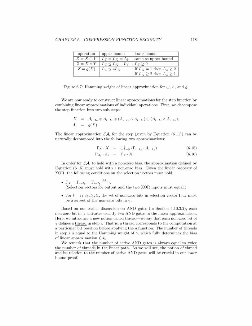
CHAPTER 6. COMPRESSION FUNCTION SECURITY 118
operation upper bound lower boundZ = X ⊕ Y LZ = LX = LY same as upper boundZ = X ∧ Y LZ ≤ LX + LY LZ ≥ 0Z = g(X) LZ ≤ 4LX If LX = 1 then LZ ≥ 2
If LX ≥ 2 then LZ ≥ 1
Figure 6.7: Hamming weight of linear approximation for ⊕, ∧, and g.
We are now ready to construct linear approximations for the step function bycombining linear approximations of individaul operations. First, we decomposethe step function into two sub-steps:
X = Ai−t0 ⊕Ai−t5 ⊕ (Ai−t1 ∧Ai−t2)⊕ (Ai−t3 ∧Ai−t4),Ai = g(X).
The linear approximation LAi for the step (given by Equation (6.11)) can benaturally decomposed into the following two approximations:
ΓX ·X = ⊕5k=0 (Γi−tk ·Ai−tk) (6.15)
ΓAi·Ai = ΓX ·X (6.16)
In order for LAi to hold with a non-zero bias, the approximation defined byEquation (6.15) must hold with a non-zero bias. Given the linear property ofXOR, the following conditions on the selection vectors must hold:
• ΓX = Γi−t0 = Γi−t5def= γ.
(Selection vectors for output and the two XOR inputs must equal.)
• For t = t1, t2, t3, t4, the set of non-zero bits in selection vector Γi−t mustbe a subset of the non-zero bits in γ.
Based on our earlier discussion on AND gates (in Section 6.10.3.2), eachnon-zero bit in γ activates exactly two AND gates in the linear approximation.Here, we introduce a new notion called thread—we say that each non-zero bit ofγ defines a thread in step i. That is, a thread corresponds to the computation ata particular bit position before applying the g function. The number of threadsin step i is equal to the Hamming weight of γ, which fully determines the biasof linear approximation LAi.
We remark that the number of active AND gates is always equal to twicethe number of threads in the linear path. As we will see, the notion of threadand its relation to the number of active AND gates will be crucial in our lowerbound proof.
CHAPTER 6. COMPRESSION FUNCTION SECURITY 119
6.10.4 Lower bound proof
6.10.4.1 Goal and approach
The goal of our analysis is to prove a lower bound on the data requirement ofany standard linear attack on the keyed MD6 compression function. In lightof earlier discussion on keyed hash functions Section 6.10.1, we will take intoaccount the effect of the security parameter λ, the number of input/output pairsthat are available to the attacker.
Similar to our approach in the differential case, the lower bound proof in thelinear case is achieved through several steps of problem reductions and facilitatedby computer-aided search.
First, deriving lower bounds on data requirement is reduced to derivingupper bounds on the total bias of a valid linear path. Then, deriving upperbounds on the total bias is reduced to deriving lower bounds on the total numberof active AND gates in the path, which is in turn reduced to deriving lowerbounds on the total number of threads (defined in Section 6.10.3.4) in the path.
In order to count the number of threads in a valid linear path, we analyzehow local linear approximations—linear approximations for a single step—canbe joined to form a valid linear path. This yields a set of necessary conditions onthe local approximations. Based on these conditions, we carry out a computer-aided search for small number of rounds. The lower bounds for small numberof rounds are then extended to produce expected lower bounds for the full rrounds of MD6 for various output sizes d.
6.10.4.2 Searching for linear path and counting threads
Recall that a linear path of MD6 is represented by a sequence of local linearapproximations for individual steps
{LAi, i = i1, i2, ...},
where each LAi is of the general form
LAi : Γi ·Ai = ⊕5k=0 (Γi−tk ·Ai−tk).
At a first glance, there seem to be many possible choices for each local ap-proximation, and so enumerating all possible linear paths is certainly infeasibleeven for very small s. Therefore, we need to eliminate as many invalid paths aspossible in the search.
A key observation is that for a linear path to be useful in launching a linearattack, the sequence of local linear approximations must “collectively” be equiv-alent to the global linear approximation of MD6 given by Equation (6.10). Thatis, all non-zero selection vectors for intermediate variables must be canceled outwith each other.
Here we elaborate on the reasoning behind this important observation forour linear cryptanalysis. Suppose that after the cancelation of intermediate
CHAPTER 6. COMPRESSION FUNCTION SECURITY 120
selection vectors, one of the internal bits, Aj [t], remains uncanceled. Then theresulting global linear aproximation would be of the form
(ΓX ·X)⊕ (ΓZ · Z)⊕Aj [t] = ΓK ⊕K,where X is the input message, K is the input secret key, and Z is the hashouput of MD6. Since the bit Aj [t] is hidden from the attacker, it would appearto be just a random bit from the attacker’s viewpoint. (Here we again use therandomness assumption about the MD6 step function.) Hence, the above globalapproximation would hold with probability 1/2 (bias zero), which would not beuseful for launching a linear attack.
The above requirement regarding cancelation helps to quickly filter out asignificant portion of the search branches in the early stage before they end upproducing an invalid linear path.
To capture the above requirement in a more analytical way and facilitatediscussion, below we introduce a few terms that distinguish different types ofselection vectors in a local linear approximation.
Consider an intermediate variable Aj . Since the step function consists of sixinputs and one output, Aj appears in the following seven steps:
step i = j, j + t0, j + t1, j + t2, j + t3, j + t4, j + t5.
If the selection vector corresponding to Aj is non-zero in the local linear ap-proximation LAi, we say that Aj gets hit in step i. Depending on the role ofAj in the step, we further categorize the hits on Aj into three different types:
• If Aj an XOR input, we say that Aj gets a hard hit.(In this case, j = i− t0 or i− t5.)
• If Aj is an AND input, we say that Aj gets a soft hit.(In this case, j = i− t1, i− t2, i− t3 or i− t4.)
• If Aj is the output of step i, we say that Aj gets a direct hit.(In this case, j = i.)
The main reason for distinguishing different types of hits is that these hitsfollow different rules of cancelation when two or more local approximationsinvolving Aj are combined. In particular, a direct hit or a hard hit must becanceled by another hit, while a soft hit can either be canceled by another hitor be “set to zero”. That is, when Aj gets a soft hit in step i, we may chooseto set the corresponding selection vector Γj = 0 if the soft hit is not neededto cancel other direct or hard hits. This would not affect the bias of the localapproximation, since all four possible approximations of AND hold with thesame bias (see discussions in Section 6.10.3.2).
Returning to our first goal of searching for valid linear paths, with the newlyintroduced terms, we can now restate the earlier requirement that “all selectionvectors for intermediate variables must be canceled out with each other” as “allthree types of hits on an intermediate variable Aj must be canceled out witheach other within the seven steps in which Aj is involved.”
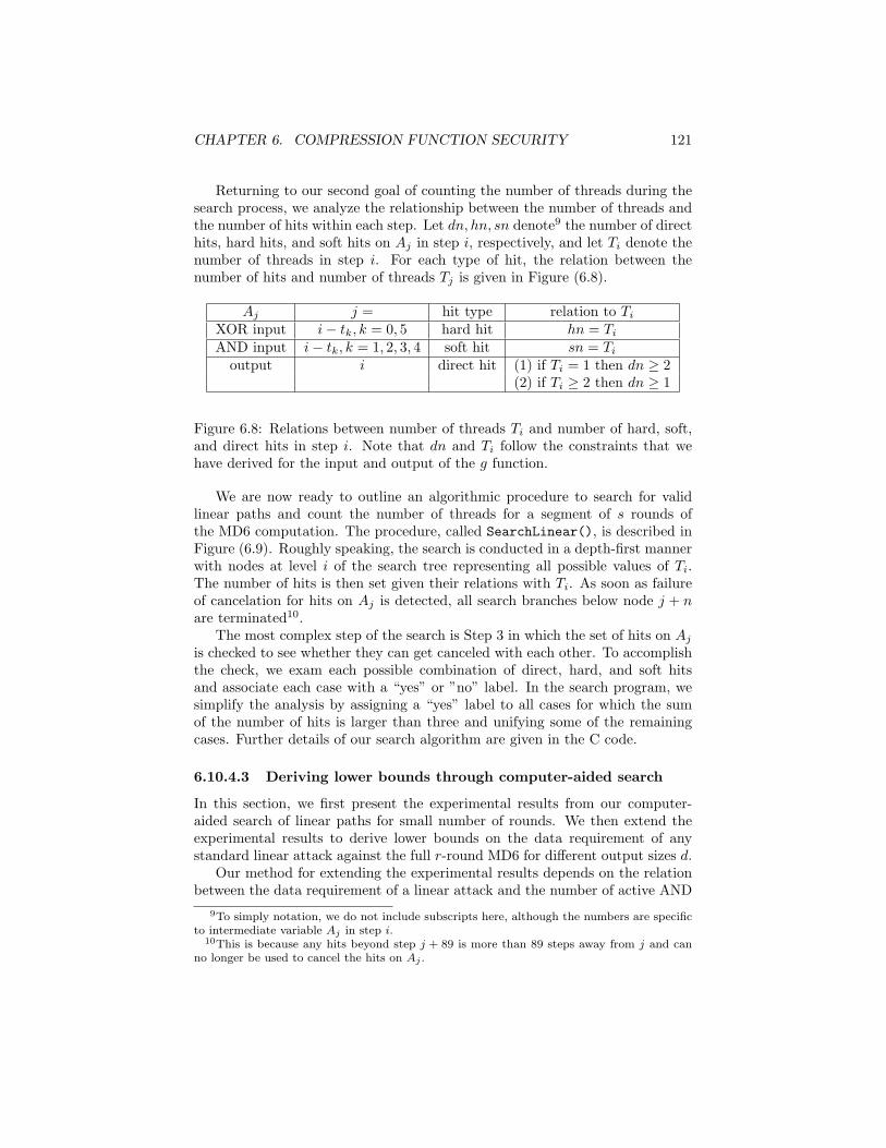
CHAPTER 6. COMPRESSION FUNCTION SECURITY 121
Returning to our second goal of counting the number of threads during thesearch process, we analyze the relationship between the number of threads andthe number of hits within each step. Let dn, hn, sn denote9 the number of directhits, hard hits, and soft hits on Aj in step i, respectively, and let Ti denote thenumber of threads in step i. For each type of hit, the relation between thenumber of hits and number of threads Tj is given in Figure (6.8).
Aj j = hit type relation to TiXOR input i− tk, k = 0, 5 hard hit hn = TiAND input i− tk, k = 1, 2, 3, 4 soft hit sn = Ti
output i direct hit (1) if Ti = 1 then dn ≥ 2(2) if Ti ≥ 2 then dn ≥ 1
Figure 6.8: Relations between number of threads Ti and number of hard, soft,and direct hits in step i. Note that dn and Ti follow the constraints that wehave derived for the input and output of the g function.
We are now ready to outline an algorithmic procedure to search for validlinear paths and count the number of threads for a segment of s rounds ofthe MD6 computation. The procedure, called SearchLinear(), is described inFigure (6.9). Roughly speaking, the search is conducted in a depth-first mannerwith nodes at level i of the search tree representing all possible values of Ti.The number of hits is then set given their relations with Ti. As soon as failureof cancelation for hits on Aj is detected, all search branches below node j + nare terminated10.
The most complex step of the search is Step 3 in which the set of hits on Ajis checked to see whether they can get canceled with each other. To accomplishthe check, we exam each possible combination of direct, hard, and soft hitsand associate each case with a “yes” or ”no” label. In the search program, wesimplify the analysis by assigning a “yes” label to all cases for which the sumof the number of hits is larger than three and unifying some of the remainingcases. Further details of our search algorithm are given in the C code.
6.10.4.3 Deriving lower bounds through computer-aided search
In this section, we first present the experimental results from our computer-aided search of linear paths for small number of rounds. We then extend theexperimental results to derive lower bounds on the data requirement of anystandard linear attack against the full r-round MD6 for different output sizes d.
Our method for extending the experimental results depends on the relationbetween the data requirement of a linear attack and the number of active AND
9To simply notation, we do not include subscripts here, although the numbers are specificto intermediate variable Aj in step i.
10This is because any hits beyond step j + 89 is more than 89 steps away from j and canno longer be used to cancel the hits on Aj .
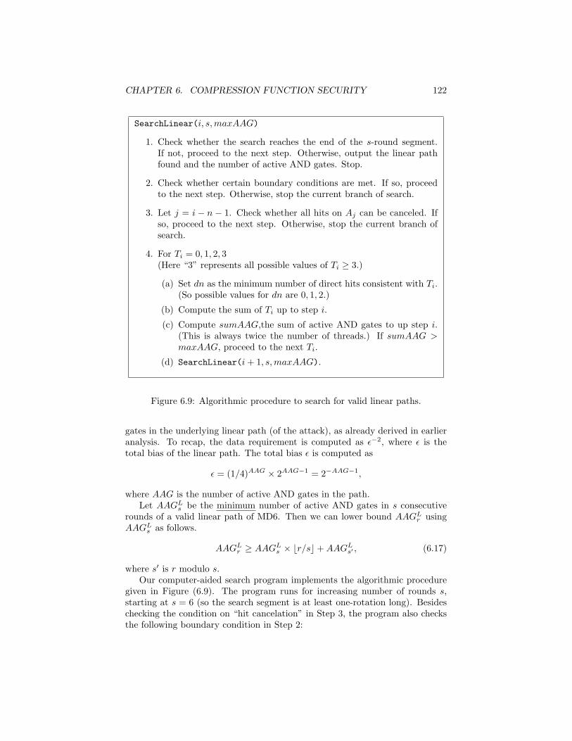
CHAPTER 6. COMPRESSION FUNCTION SECURITY 122
SearchLinear(i, s,maxAAG)
1. Check whether the search reaches the end of the s-round segment.If not, proceed to the next step. Otherwise, output the linear pathfound and the number of active AND gates. Stop.
2. Check whether certain boundary conditions are met. If so, proceedto the next step. Otherwise, stop the current branch of search.
3. Let j = i − n − 1. Check whether all hits on Aj can be canceled. Ifso, proceed to the next step. Otherwise, stop the current branch ofsearch.
4. For Ti = 0, 1, 2, 3(Here “3” represents all possible values of Ti ≥ 3.)
(a) Set dn as the minimum number of direct hits consistent with Ti.(So possible values for dn are 0, 1, 2.)
(b) Compute the sum of Ti up to step i.
(c) Compute sumAAG,the sum of active AND gates to up step i.(This is always twice the number of threads.) If sumAAG >maxAAG, proceed to the next Ti.
(d) SearchLinear(i+ 1, s,maxAAG).
Figure 6.9: Algorithmic procedure to search for valid linear paths.
gates in the underlying linear path (of the attack), as already derived in earlieranalysis. To recap, the data requirement is computed as ε−2, where ε is thetotal bias of the linear path. The total bias ε is computed as
ε = (1/4)AAG × 2AAG−1 = 2−AAG−1,
where AAG is the number of active AND gates in the path.Let AAGLs be the minimum number of active AND gates in s consecutive
rounds of a valid linear path of MD6. Then we can lower bound AAGLr usingAAGLs as follows.
AAGLr ≥ AAGLs × br/sc+AAGLs′ , (6.17)
where s′ is r modulo s.Our computer-aided search program implements the algorithmic procedure
given in Figure (6.9). The program runs for increasing number of rounds s,starting at s = 6 (so the search segment is at least one-rotation long). Besideschecking the condition on “hit cancelation” in Step 3, the program also checksthe following boundary condition in Step 2:
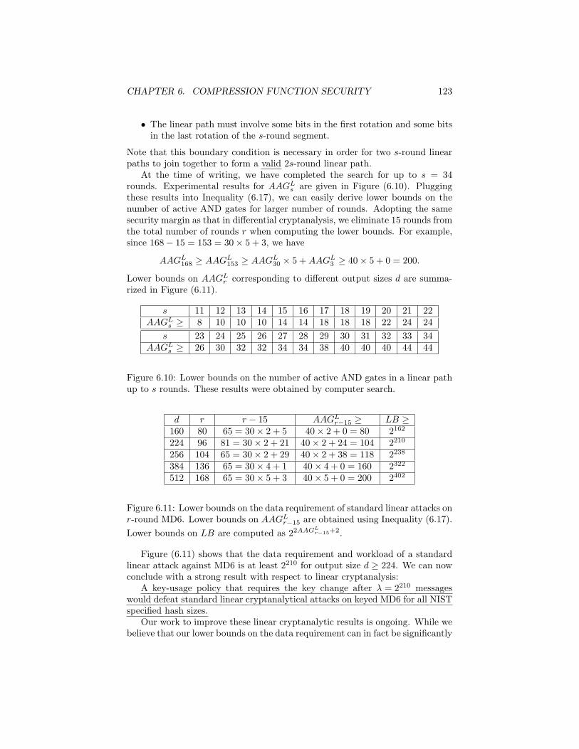
CHAPTER 6. COMPRESSION FUNCTION SECURITY 123
• The linear path must involve some bits in the first rotation and some bitsin the last rotation of the s-round segment.
Note that this boundary condition is necessary in order for two s-round linearpaths to join together to form a valid 2s-round linear path.
At the time of writing, we have completed the search for up to s = 34rounds. Experimental results for AAGLs are given in Figure (6.10). Pluggingthese results into Inequality (6.17), we can easily derive lower bounds on thenumber of active AND gates for larger number of rounds. Adopting the samesecurity margin as that in differential cryptanalysis, we eliminate 15 rounds fromthe total number of rounds r when computing the lower bounds. For example,since 168− 15 = 153 = 30× 5 + 3, we have
AAGL168 ≥ AAGL153 ≥ AAGL30 × 5 +AAGL3 ≥ 40× 5 + 0 = 200.
Lower bounds on AAGLr corresponding to different output sizes d are summa-rized in Figure (6.11).
s 11 12 13 14 15 16 17 18 19 20 21 22AAGLs ≥ 8 10 10 10 14 14 18 18 18 22 24 24
s 23 24 25 26 27 28 29 30 31 32 33 34AAGLs ≥ 26 30 32 32 34 34 38 40 40 40 44 44
Figure 6.10: Lower bounds on the number of active AND gates in a linear pathup to s rounds. These results were obtained by computer search.
d r r − 15 AAGLr−15 ≥ LB ≥160 80 65 = 30× 2 + 5 40× 2 + 0 = 80 2162
224 96 81 = 30× 2 + 21 40× 2 + 24 = 104 2210
256 104 65 = 30× 2 + 29 40× 2 + 38 = 118 2238
384 136 65 = 30× 4 + 1 40× 4 + 0 = 160 2322
512 168 65 = 30× 5 + 3 40× 5 + 0 = 200 2402
Figure 6.11: Lower bounds on the data requirement of standard linear attacks onr-round MD6. Lower bounds on AAGLr−15 are obtained using Inequality (6.17).Lower bounds on LB are computed as 22AAGL
r−15+2.
Figure (6.11) shows that the data requirement and workload of a standardlinear attack against MD6 is at least 2210 for output size d ≥ 224. We can nowconclude with a strong result with respect to linear cryptanalysis:
A key-usage policy that requires the key change after λ = 2210 messageswould defeat standard linear cryptanalytical attacks on keyed MD6 for all NISTspecified hash sizes.
Our work to improve these linear cryptanalytic results is ongoing. While webelieve that our lower bounds on the data requirement can in fact be significantly
CHAPTER 6. COMPRESSION FUNCTION SECURITY 124
improved, we note that it does not actually need to be so improved in order toprovide security against massive linear cryptanalysis attacks, as long as a key-usage policy such as the above is enforced.
(We note that if someone wishes to use keyed MD6 for d-bit MAC com-putations where d ≤ 160, we recommend that they keep r = 80, rather thanallowing r to decrease to 40 as d approaches 1 as is done for unkeyed usage ofMD6. That is, in such cases the output length may not be a good determinantof the desired security level, since we are now worried about key protectionrather than collision-resistance. Requiring r ≥ 80 appears to provide adequateprotection against linear cryptanalysis attacks, for example, even for very shortoutput lengths. Further analysis might show that fewer rounds are also safe, butfor now a recommended minimum of 80 rounds seems a conservative approach.The default number of rounds for MD6 follows this approach.)
In sum, decoupling the key-usage parameter λ from the other security pa-rameters d and r is, we feel, a significant and useful way to proceed. Hence,even with the preliminary results given in this report, we have demonstratedthat in this expanded analysis framework, MD6 offers strong security againstlinear cryptanalysis attacks.
6.10.4.4 Related work
Our lower bound proof with respective to linear cryptanalysis is also similarto that of the AES [33]. The proof that AES is secure against standard linearattacks goes as follows:
• Each active S-box in AES has a maximum input/output correlation of atmost 2−3.
• In four consecutive rounds of AES, there are at least 25 active S-boxes.
• So the input/output correlation of any four-round linear path is at most2−75, implying a data requirement of at least 2150 to launch a standardlinear attack.
Finally, we remark that active AND gates in MD6 play the same role toactive S-boxes in AES with respect to linear cryptanalysis. The g operator inMD6 also has some limited effect in terms of enforcing a small number of activeAND gates across two consecutive steps, although it does not directly compareto the strong diffusion property of the MDS matrix.
6.11 Algebraic attacks
There are a number of algebraic attacks one might consider trying against theMD6 compression function.
CHAPTER 6. COMPRESSION FUNCTION SECURITY 125
6.11.1 Degree Estimates
Many algebraic attacks, such as Shamir’s “cube” attack, require that the al-gebraic normal form describing the output bits have relatively small degree interms of the input bits being considered. There are 89 · 64 = 5696 input vari-ables, one for each of the 64 bits in each of the 89 input words to the compressionfunction f . A particular algebraic attack may consider only a subset of these,and leave the others fixed.
Each bit of each word A[i] is a function of the nw = 5696 input variables,that can be described in a unique way by a polynomial in algebraic normalform (ANF). A particular MD6 output bit can be represented in a unique wayas an ANF polynomial with input variables x1, x2, . . . , xnw and coefficients andoutputs in GF (2), e.g.
a0 ⊕ a1x1 ⊕ . . . ⊕ anwxnw ⊕ anw+1x1x2 ⊕ . . . ⊕ a2nw−1x1x2 · · ·xnw . (6.18)
There are 2nw terms in this sum, one for each subset of the variables. Thecoefficient for a term determines whether that term is “present” (coefficient =1) or “absent” (coefficient = 0).
6.11.1.1 Maximum degree estimates
We can estimate the degree of the polynomial for such bit in A[i] as follows. Weestimate a common degree of the polynomials for each of the 64 bits occuringword A[i]. Let δi to denote the estimated common degree for bits in A[i]:
δi = 1 for i = 0, 1, . . . , n− 1 (6.19)
and
δi = min(δi−t5 , δi−t0 , χ(δi−t1 , δi−t2), χ(δi−t3 , δi−t4)) for i > 88 ,
whereχ(d1, d2) = d1 + d2 − d1d2/nw .
(The term d1d2/nw accounts for the fact that random terms of degree d1 and d2
should have about d1d2/nw variables in common, so the degree of their productwill be smaller by this amount than the sum d1 + d2 of their degrees.) Weobtain the following estimate for the minimum degree of any bit computed ineach round.
According to these estimates (see Table 6.4), after 12 rounds the minimumdegree should easily exceed 512, and after 20 rounds the minimum degree shouldalmost certainly equal the maximum possible degree nw = 5696.
Similar computations can be performed when one cares about only some ofthe input variables (i.e., when some of the variables are fixed, and we only careabout the degree in terms of the remaining variables).
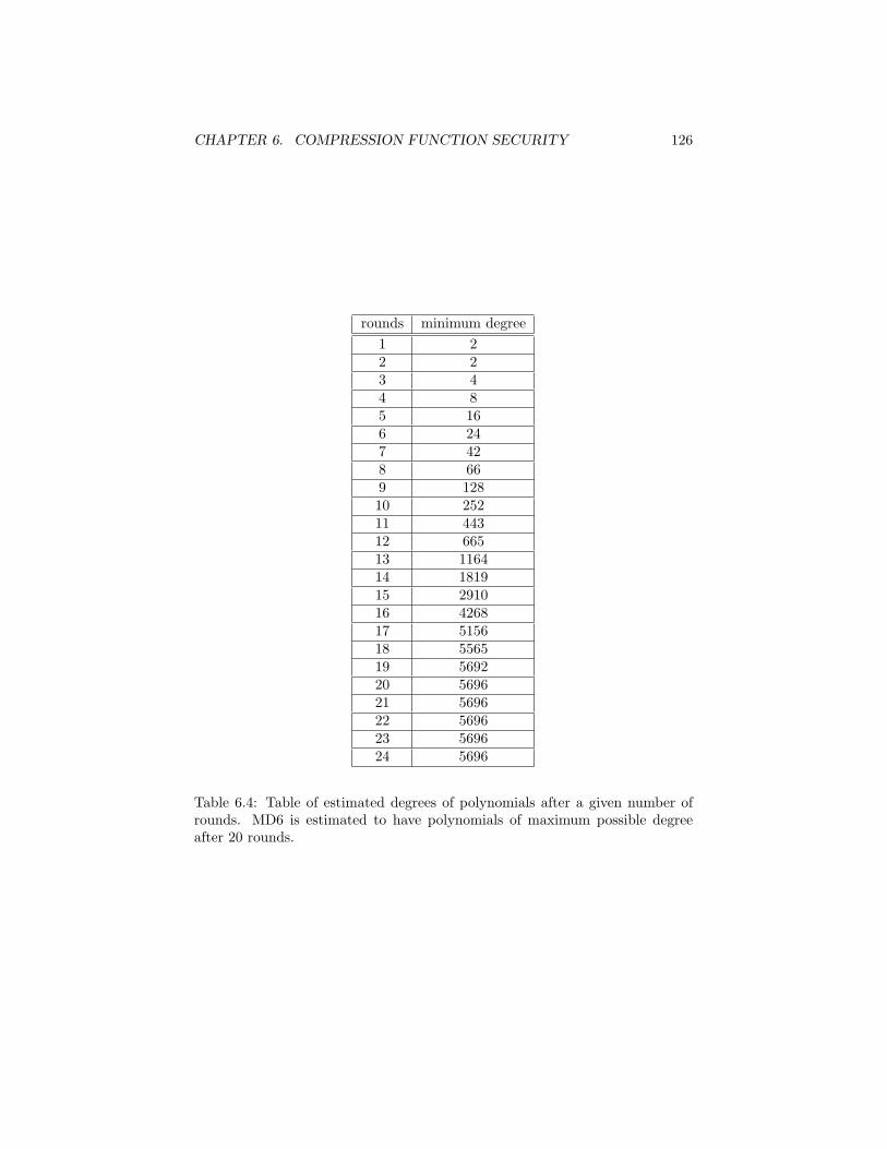
CHAPTER 6. COMPRESSION FUNCTION SECURITY 126
rounds minimum degree1 22 23 44 85 166 247 428 669 12810 25211 44312 66513 116414 181915 291016 426817 515618 556519 569220 569621 569622 569623 569624 5696
Table 6.4: Table of estimated degrees of polynomials after a given number ofrounds. MD6 is estimated to have polynomials of maximum possible degreeafter 20 rounds.
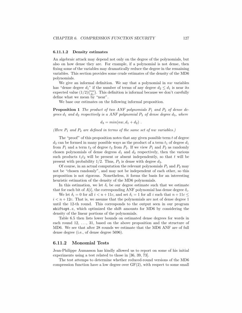
CHAPTER 6. COMPRESSION FUNCTION SECURITY 127
6.11.1.2 Density estimates
An algebraic attack may depend not only on the degree of the polynomials, butalso on how dense they are. For example, if a polynomial is not dense, thenfixing some of the variables may dramatically reduce the degree in the remainingvariables. This section provides some crude estimates of the density of the MD6polynomials.
We give an informal definition. We say that a polynomial in nw variableshas “dense degree d1” if the number of terms of any degree d2 ≤ d1 is near itsexpected value (1/2)
(nwd2
). This definition is informal because we don’t carefully
define what we mean by “near”.We base our estimates on the following informal proposition.
Proposition 1 The product of two ANF polynomials P1 and P2 of dense de-grees d1 and d2 respectively is a ANF polynomial P3 of dense degree d3, where
d3 = min(nw, d1 + d2) .
(Here P1 and P2 are defined in terms of the same set of nw variables.)
The “proof” of this proposition notes that any given possible term t of degreed3 can be formed in many possible ways as the product of a term t1 of degree d1
from P1 and a term t2 of degree t2 from P2. If we view P1 and P2 as randomlychosen polynomials of dense degress d1 and d2 respectively, then the varioussuch products t1t2 will be present or absent independently, so that t will bepresent with probability 1/2. Thus, P3 is dense with degree d3.
Of course, in an actual computation the relevant polynomials P1 and P2 maynot be “chosen randomly”, and may not be independent of each other, so thisproposition is not rigorous. Nonetheless, it forms the basis for an interestingheuristic estimation of the density of the MD6 polynomials.
In this estimation, we let δi be our degree estimate such that we estimatethat for each bit of A[i], the corresponding ANF polynomial has dense degree δi.
We let δi = 0 for all i < n+ 11c, and set δi = 1 for all i such that n+ 11c ≤i < n+ 12c. That is, we assume that the polynomials are not of dense degree 1until the 12-th round. This corresponds to the output seen in our programshiftopt.c, which optimized the shift amounts for MD6 by considering thedensity of the linear portions of the polynomials.
Table 6.5 then lists lower bounds on estimated dense degrees for words ineach round 12, . . . , 31, based on the above proposition and the structure ofMD6. We see that after 28 rounds we estimate that the MD6 ANF are of fulldense degree (i.e., of dense degree 5696).
6.11.2 Monomial Tests
Jean-Philippe Aumasson has kindly allowed us to report on some of his initialexperiments using a test related to those in [36, 39, 73].
The test attemps to determine whether reduced-round versions of the MD6compression function have a low degree over GF(2), with respect to some small
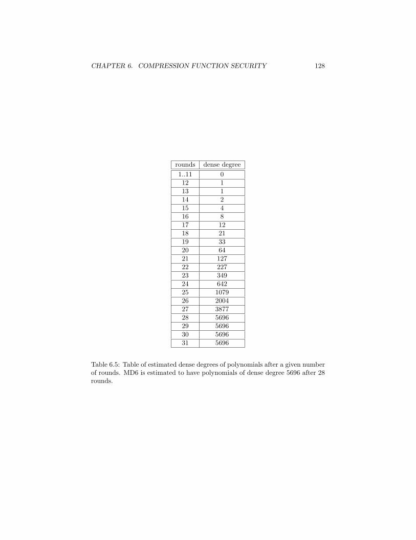
CHAPTER 6. COMPRESSION FUNCTION SECURITY 128
rounds dense degree1..11 012 113 114 215 416 817 1218 2119 3320 6421 12722 22723 34924 64225 107926 200427 387728 569629 569630 569631 5696
Table 6.5: Table of estimated dense degrees of polynomials after a given numberof rounds. MD6 is estimated to have polynomials of dense degree 5696 after 28rounds.
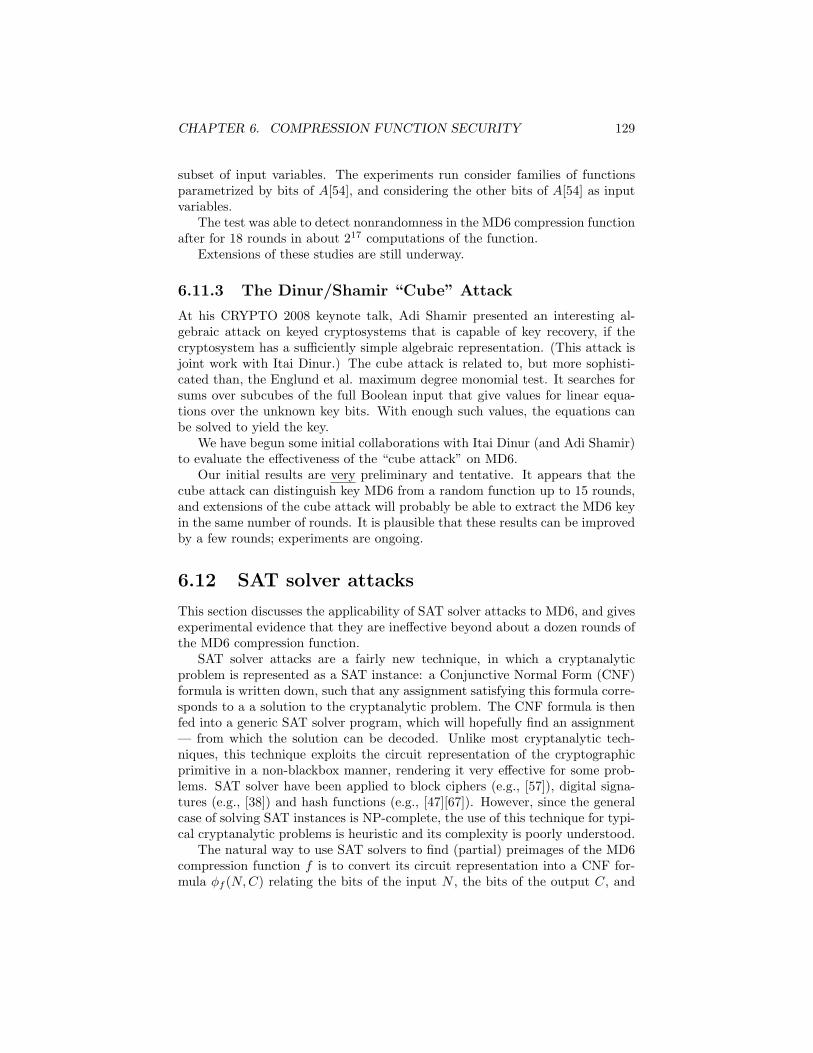
CHAPTER 6. COMPRESSION FUNCTION SECURITY 129
subset of input variables. The experiments run consider families of functionsparametrized by bits of A[54], and considering the other bits of A[54] as inputvariables.
The test was able to detect nonrandomness in the MD6 compression functionafter for 18 rounds in about 217 computations of the function.
Extensions of these studies are still underway.
6.11.3 The Dinur/Shamir “Cube” Attack
At his CRYPTO 2008 keynote talk, Adi Shamir presented an interesting al-gebraic attack on keyed cryptosystems that is capable of key recovery, if thecryptosystem has a sufficiently simple algebraic representation. (This attack isjoint work with Itai Dinur.) The cube attack is related to, but more sophisti-cated than, the Englund et al. maximum degree monomial test. It searches forsums over subcubes of the full Boolean input that give values for linear equa-tions over the unknown key bits. With enough such values, the equations canbe solved to yield the key.
We have begun some initial collaborations with Itai Dinur (and Adi Shamir)to evaluate the effectiveness of the “cube attack” on MD6.
Our initial results are very preliminary and tentative. It appears that thecube attack can distinguish key MD6 from a random function up to 15 rounds,and extensions of the cube attack will probably be able to extract the MD6 keyin the same number of rounds. It is plausible that these results can be improvedby a few rounds; experiments are ongoing.
6.12 SAT solver attacks
This section discusses the applicability of SAT solver attacks to MD6, and givesexperimental evidence that they are ineffective beyond about a dozen rounds ofthe MD6 compression function.
SAT solver attacks are a fairly new technique, in which a cryptanalyticproblem is represented as a SAT instance: a Conjunctive Normal Form (CNF)formula is written down, such that any assignment satisfying this formula corre-sponds to a a solution to the cryptanalytic problem. The CNF formula is thenfed into a generic SAT solver program, which will hopefully find an assignment— from which the solution can be decoded. Unlike most cryptanalytic tech-niques, this technique exploits the circuit representation of the cryptographicprimitive in a non-blackbox manner, rendering it very effective for some prob-lems. SAT solver have been applied to block ciphers (e.g., [57]), digital signa-tures (e.g., [38]) and hash functions (e.g., [47][67]). However, since the generalcase of solving SAT instances is NP-complete, the use of this technique for typi-cal cryptanalytic problems is heuristic and its complexity is poorly understood.
The natural way to use SAT solvers to find (partial) preimages of the MD6compression function f is to convert its circuit representation into a CNF for-mula φf (N,C) relating the bits of the input N , the bits of the output C, and
CHAPTER 6. COMPRESSION FUNCTION SECURITY 130
some ancillary bits for the intermediate state of the compression function. Onethen extend φf (N,C) with further clauses restricting C to a desired value andexpressing any desired constraints on N , and solves this instance to obtain thefull input N . Similarly, to find an arbitrary pair of colliding inputs N,N ′, onecan use the formula φf (N,C) ∧ φf (N ′, C) ∧ (Ni ∨ N ′i) ∧ (Ni ∨ N ′i), where i isthe index of some bit forced to differ between N and N ′.
Following this approach, we used a Python script to create a variety ofCNF instances representing generic attacks on the MD6 compression function.In particular, we explored the following variants (the notation is used in thesubsequent figures):
1. Task: finding a preimage of the all-zero output (invert) or finding anarbitrary collision of two inputs differing in a specific bit (collide).
2. Digest length: d=128, d=160, d=224, d=256, d=384 or d=512.
3. Constraints on the sought compression function input: only Q fixed to itsprescribed
√6 value (fix=Q), only Q fixed to 0 (fix=Q0), or all of Q, K,
U and V fixed to values corresponding to the first block in a long message(fix=QKUV).
To solve these SAT instances, we used Minisat2 beta 070721 (including itssimplification preprocessing), which is one of the best general-purpose SATsolvers available and is popular in cryptanalytic context. We have also evaluatedHaifaSat, march, picosat-632, rsat and SATzilla; these consistently performedworse than Minisat2 on our problem instances (for non-trivial problem sizes).In both figures, the lower cluster corresponds to the invert instances, whereasthe upper cluster corresponds to the collide instances.11
Figures 6.12 and 6.13 summarize the running time and memory consump-tion of Minisat on all of the above instances. For ease of visualization, failedexecutions are always listed as running for 1000 seconds and consuming 1GB(no trial succeeded after using more than either of these).
These experiments were run on a Dual-Core AMD Opteron 221 (2.4GHz)with 2GB of DRAM running Linux under Xen. Available memory was initiallyconstrainted to 1GB. When Minisat2 failed to solve a given instance withinthe allotted 1GB of memory, we increased the memory limit to about 1.5GBand also patched Minisat2 to reduce its memory use in exchange for a longerrunning time (by setting the internal variables learntsize factor=0.2 andlearntsize inc=1.02). In all of the above cases, the modified Minisat was stillunable to solve these instances within the allotted memory.
As can be seen, our method of using SAT solvers to attack Minisat succeededfor no more than r = 10 rounds at the standard SHA-3 digest sizes (d ≥ 224),and at most r = 11 rounds even for reduced digest sizes (d = 128 and d = 160).Moreover, after 6-7 rounds, both running time and memory usage appear togrow superexponentially in the number of rounds. While varying the CNF
11One would expect finding collisions to be easier than inversion, but apparently the SATsolver is bogged down by the larger number of variables.
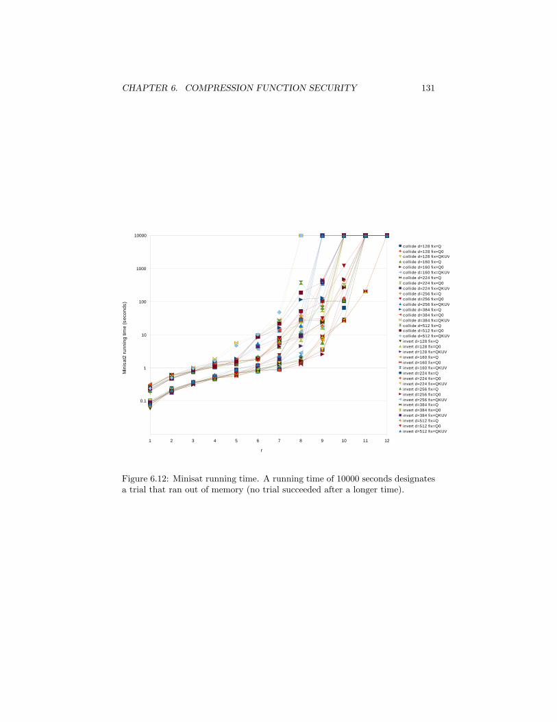
CHAPTER 6. COMPRESSION FUNCTION SECURITY 131
1 2 3 4 5 6 7 8 9 10 11 12
0.1
1
10
100
1000
10000
col l ide d=128 fix=Qcol lide d=128 fix=Q0col l ide d=128 fix=QKUVcol lide d=160 fix=Qcol lide d=160 fix=Q0col l ide d=160 fix=QKUVcol lide d=224 fix=Qcol lide d=224 fix=Q0col l ide d=224 fix=QKUVcol lide d=256 fix=Qcol lide d=256 fix=Q0col l ide d=256 fix=QKUVcol lide d=384 fix=Qcol lide d=384 fix=Q0col l ide d=384 fix=QKUVcol lide d=512 fix=Qcol lide d=512 fix=Q0col l ide d=512 fix=QKUVinvert d=128 fix=Qinvert d=128 fix=Q0invert d=128 fix=QKUVinvert d=160 fix=Qinvert d=160 fix=Q0invert d=160 fix=QKUVinvert d=224 fix=Qinvert d=224 fix=Q0invert d=224 fix=QKUVinvert d=256 fix=Qinvert d=256 fix=Q0invert d=256 fix=QKUVinvert d=384 fix=Qinvert d=384 fix=Q0invert d=384 fix=QKUVinvert d=512 fix=Qinvert d=512 fix=Q0invert d=512 fix=QKUV
r
Min
isa
t2 r
un
nin
g ti
me
(s
eco
nd
s)
Figure 6.12: Minisat running time. A running time of 10000 seconds designatesa trial that ran out of memory (no trial succeeded after a longer time).
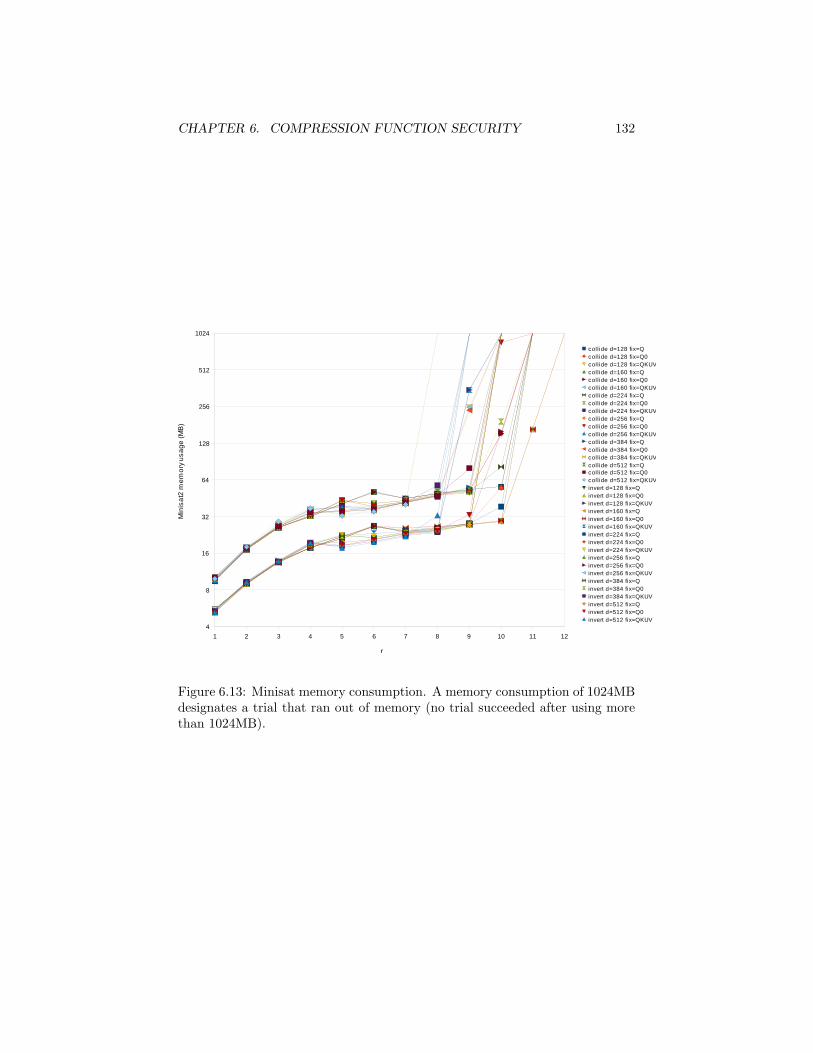
CHAPTER 6. COMPRESSION FUNCTION SECURITY 132
1 2 3 4 5 6 7 8 9 10 11 12
4
8
16
32
64
128
256
512
1024
col l ide d=128 fix=Qcol lide d=128 fix=Q0col l ide d=128 fix=QKUVcol lide d=160 fix=Qcol lide d=160 fix=Q0col l ide d=160 fix=QKUVcol lide d=224 fix=Qcol lide d=224 fix=Q0col l ide d=224 fix=QKUVcol lide d=256 fix=Qcol lide d=256 fix=Q0col l ide d=256 fix=QKUVcol lide d=384 fix=Qcol lide d=384 fix=Q0col l ide d=384 fix=QKUVcol lide d=512 fix=Qcol lide d=512 fix=Q0col l ide d=512 fix=QKUVinvert d=128 fix=Qinvert d=128 fix=Q0invert d=128 fix=QKUVinvert d=160 fix=Qinvert d=160 fix=Q0invert d=160 fix=QKUVinvert d=224 fix=Qinvert d=224 fix=Q0invert d=224 fix=QKUVinvert d=256 fix=Qinvert d=256 fix=Q0invert d=256 fix=QKUVinvert d=384 fix=Qinvert d=384 fix=Q0invert d=384 fix=QKUVinvert d=512 fix=Qinvert d=512 fix=Q0invert d=512 fix=QKUV
r
Min
isa
t2 m
em
ory
us
ag
e (
MB
)
Figure 6.13: Minisat memory consumption. A memory consumption of 1024MBdesignates a trial that ran out of memory (no trial succeeded after using morethan 1024MB).
CHAPTER 6. COMPRESSION FUNCTION SECURITY 133
circuit representation and the choice of SAT solver program may somewhatalter these numbers, it typically does not have a dramatic effect. We thusconclude that at the current state of the art in SAT solvers, this form of SATsolver attack is ineffective against the full MD6 compression function.
6.13 Number of rounds
Given the studies and tests of the preceding sections, it is appropriate to revisitthe question of the number of rounds that is appropriate for MD6.
None of our tests are able to distinguish MD6 with 11 or more rounds froma random function. Jean-Philippe Aumasson’s test of Section 6.11.2 can distin-guish MD6 from a random function up to 18 rounds, but not more (at least atpresent).
Our choice of r = 40 + (d/4) rounds as the default thus seems quite conser-vative.
Perhaps after further study, the default number of rounds for MD6 could bejustifiably and significantly reduced.
6.14 Summary
The compression function of MD6 appears to have all of the desired proper-ties: preimage-resistance, second-preimage resistance, collision-resistance, pseu-dorandomness, resistance to linear and differential attacks, resistance to SAT-solver attacks, and indifferentiability from a random oracle. It provides anexcellent foundation on which to build the complete MD6 hash function usingthe MD6 mode of operation.
Chapter 7
Mode of Operation Security
A mode of operation M is an algorithm that, given a fixed-length com-pression function or block cipher fQ, describes how to apply fQ repeatedly onfixed-length chunks of the arbitrarily-sized input in order to produce a fixed-length output for the whole. In this way, one can construct Variable InputLength (VIL) cryptographic primitives from Fixed Input Length (FIL) cryp-tographic primitives, which is a functionality commonly referred to as domainextension [35].
In this chapter we address the cryptographic properties of collision resis-tance, first-preimage resistance, second-preimage resistance, psuedorandomness,unpredictability, and indifferentiability from random oracles, as pertains partic-ularly to the MD6 mode of operation itself1. That is, in this chapter we take anagnostic approach to the compression function used and consider it as only ablack-box function fQ with some desirable property P (e.g. collision resistance,pseudorandomness, etc.). Our goal is then to show that the MD6 mode of op-eration acts as a domain extender for fQ that preserves the property P . Thequestion we attempt to answer is, does the MD6 mode of operation dilute the se-curity of the black-box function with respect to P , and if so, by how much? Forcollision resistance, first-preimage resistance, pseudorandomness, and indiffer-entiability we give concrete security bounds for the property preservation. Forthe MAC functionality (unpredictability), we do the same, although we mustintroduce an additional nontrivial assumption on the compression function. Forthe property of second-preimage resistance, we are unable to demonstrate prov-ably that it preserves this property (although we reduce to a weaker propertyinstead).
The organization of this chapter is as follows. After some preliminary re-marks in Section 7.1, Sections 7.2, 7.3, 7.4 respectively show how the MD6 modeof operation is a domain extender for collision-resistance, preimage-resistance(inversion resistance), and second-preimage resistance. Then Section 7.5 uses
1Many of the results presented here were derived by Christopher Crutchfield in his MITEECS Master’s thesis [32]; we summarize those results here but refer the reader to the thesisfor the full exposition and derivation.
134
CHAPTER 7. MODE OF OPERATION SECURITY 135
Mauer’s Random Systems Framework to show that the MD6 mode of operationis a domain extender for pseudo-random functions. The more delicate issueof showing that the MD6 mode of operation is a domain extender for unpre-dictability is handled in Section 7.6. Section 7.7 shows that the MD6 mode ofoperation provides indifferentiability of MD6 from a random oracle assumingthat the compression function is a random oracle (and that the adversary hasaccess to the compression function). Sections 7.8 and 7.9 discuss, in responseto NIST requirements, the issues of multi-collision attacks and length-extensionattacks. Section 7.10 then summarizes the results of this chapter.
7.1 Preliminaries
In this section we prove certain results about the collision and preimage resis-tance of the MD6 hash function mode of operation. In particular, we show thatthe MD6 mode of operation acts as a domain extender for various propertiesof the fixed input length compression function used. Our goal is to show thatif we assume that the compression function is collision resistant (respectively,preimage resistant), then the entire hash function will be collision resistant (re-spectively, preimage resistant) as well.
One important caveat is that the notions of collision resistance and preim-age resistance are only defined for keyed hash functions. As observed by Ro-gaway [86], an unkeyed hash function H : {0, 1}∗ → {0, 1}d is trivially non-collision resistant: the existence of an efficient algorithm that can find distinctstrings M and M ′ such that H(M) = H(M ′) is guaranteed, simply by virtue ofthe existence of such collisions (as Rogaway says, the algorithm has the collision“hardwired in”). Therefore for an unkeyed hash function H, what is meantby saying that H is collision resistant is not that an efficient collision-findingalgorithm does not exist, but rather that no efficient collision-finding algorithmexists that is known to man (the emphasis is Rogaway’s). Similar concernscan also be expressed for the preimage resistance of unkeyed hash functions.Although MD6 can behave as a keyed hash function, certain applications callfor the use of the unkeyed variant (where the key field is simply set to λ, theempty string), such as any application that uses a public hash function. Thuswe would like to argue, with some amount of rigor, that its unkeyed variant iscollision or preimage resistant as well.
Fortunately, we can perform reductions for finding collisions and preimages.Specifically, we will show that if one has a collision or preimage for the entirehash, then one can construct a collision or preimage for the underlying compres-sion function. Therefore if one assumes that there is no known algorithm forfinding collisions or preimages in the compression function, then there shouldbe no known algorithm for finding collisions or preimages in the overall hashfunction. While this is not a completely rigorous notion of security (as it relieson the extent of human knowledge for finding collisions, which is impossible toformalize), it is the best we can do in these circumstances.
After proving reductions for these properties, we show that they apply to
CHAPTER 7. MODE OF OPERATION SECURITY 136
the keyed hash function variant of MD6 as well (for certain — now rigorous— definitions of collision resistance and preimage resistance). That is, we willdemonstrate that if an algorithm exists that can break the property of collisionresistance or preimage resistance for keyed MD6, then we can use this algorithmas a black box for breaking the collision resistance or preimage resistance ofthe underlying compression function. We may then conclude that breakingeither property is at least as difficult as breaking the respective property for thecompression function.
Some of the proofs in this section are similar to those of Sarkar and Schel-lenberg [88], owing to the fact that their mode of operation is also based ona tree-like construction. However, the differences between the MD6 mode ofoperation and that of Sarkar and Schellenberg are significant enough to warrantentirely new proofs of security.
7.1.1 Definitions
We will often use the following notational conventions when precisely definingthe advantage of an adversary for attacking some cryptographic property of thecompression function or hash function.
AdvPA = Pr
Random values are chosen;A is given these values as input;
A produces some output: A’s output violates P
For example, one definition of the advantage of A for breaking the collision
resistance of fQ is due to Rogaway and Shrimpton [87].
Advfil-crA = Pr
[K
$← {0, 1}k;(m,m′)← A(K)
:m 6= m′,
fQ(K,m) = fQ(K,m′)
]
Here the probability is taken over the uniform random choice of key valueK from the keyspace {0, 1}k (where this random choice is denoted by $). To bemore precise, we should also take into account the internal randomness of thealgorithm A, which in general is not a deterministic algorithm. We could denotethis similarly as (m,m′) $← A(K), but throughout this paper we will often takethis as a given and omit the $.
Definition 3 (Fixed Input Length) A function fQ mapping domain D to Ris a fixed input length (FIL) function if D = {0, 1}i for some positive integer i.That is, its inputs consist only of bit strings of some fixed length.
Definition 4 (Variable Input Length) A function H mapping domain D toR is a variable input length (VIL) function if D = {0, 1}∗. That is, its inputsare bit strings of variable length.
CHAPTER 7. MODE OF OPERATION SECURITY 137
Definition 5 (Domain Extender) We say some algorithm A is a domainextender for property P if, given a fixed input length function fQ that is FIL-P(that is, has the property of P for fixed input length), then Af (A when givenoracle access to fQ) is a variable input length function that has the property ofVIL-P (that is, it has the property of P for variable input length).
Note that traditionally a domain extender only extends the domain of thefunction and provides no guarantees that the new function satisfies any proper-ties. However, in our context we will mean that A is a domain extender and aproperty P preserver.
Definition 6 (Running Time) Oftentimes we will say that an algorithm Ahas “running time” t. By this we mean that t includes both the amount of timetaken by an invocation of A as well as the size of the code implementing A,measured in some fixed RAM model of computation (as in [3]).
Definition 7 (Mode of Operation) Throughout this chapter we will use Mto denote MD6’s mode of operation. This is defined irrespective of the compres-sion function used, although we will often use MfQ : Wk × {0, 1}∗ → {0, 1}dto denote the MD6 mode of operation applied to the compression function fQ(i.e. MfQ(M) is the MD6 hash of a message M), the superscript denoting thatthe mode of operation only makes black-box use of fQ. When needed, we willparameterize MfQ by L, denoting this as MfQ
L .On occasion we will consider the output of MfQ without the final compres-
sion function application. Recall that the final compression function has thez bit set to 1, and then its output is chopped from c words down to d bits.Therefore we write the mode of operation without the final compression functionapplication as HfQ : Wk × {0, 1}∗ →Wn−q−k, where
MfQ = χd ◦ f ◦ HfQ .
Recall that the chop function χd : {0, 1}∗ → {0, 1}d operates simply by returningthe last d-bits of its input. We can abbreviate the action of the final compressionfunction and the chop by defining g = (χd ◦ fQ) : Wk ×Wn−q−k → {0, 1}d.
Definition 8 (Height) For a given maximum level parameter L, let the heightof the MD6 hash tree parameterized by L on a message M of length µ = |M | begiven as heightL(µ). Recall that the height of a tree is given by the distance ofthe root node from the farthest leaf node. For example, the tree in Figure 2.1has height 3, the tree in Figure 2.3 has height 6, and the tree in Figure 2.2 hasheight 18.
Oftentimes we will have some adversary A that we grant q queriesM1, . . . ,Mq
to the MD6 hash algorithmMfQ , where we bound the total length of the queries,∑i |Mi| ≤ µ. One question we might ask is, in the course of execution ofMfQ ,
how many queries to fQ will need to be made, given the above resource con-straints?
CHAPTER 7. MODE OF OPERATION SECURITY 138
Lemma 2 Assume we are given oracle access to fQ(K, ·) for some K. Then ifwe have q messages M1,M2, . . . ,Mq such that
q∑i=1
|Mi| ≤ µ,
then in order to compute Di =MfQ(K,·)L (Mi) for all i we require at most δ(q, µ)
queries to the oracle fQ(K, ·), where
δ(q, µ) =13·⌈µc
⌉+ q log4
(1q·⌈µc
⌉)+q
3.
Proof: The proof of this lemma is fairly straightforward, so we refer theinterested reader to Lemma 2.1 of [32]
7.2 Collision-Resistance
To begin, we first define what it means for a keyed fixed input length (FIL)compression function fQ to be collision resistant, and what it means for a keyedvariable input length (VIL) hash function H to be collision resistant.
Definition 9 (FIL-Collision Resistance) For a keyed FIL function fQ map-ping Wk ×Wn−q−k →Wc, define the advantage of an adversary A for findinga collision as
Advfil-crA = Pr
[K
$←Wk;(m,m′)← A(K)
:m 6= m′,
fQ(K,m) = fQ(K,m′)
]
We define the insecurity of fQ with respect to FIL-collision resistance (FIL-CR)as
InSecfil-crfQ
(t) = maxA
{Advfil-cr
A
},
where the maximum is taken over all adversaries A with total running time t.
Definition 10 (VIL-Collision Resistance) For a keyed VIL function H map-ping Wk×{0, 1}∗ → {0, 1}d, define the advantage of an adversary A for findinga collision as
Advvil-crA = Pr
[K
$←Wk;(M,M ′)← A(K)
:M 6= M ′,
H(K,M) = H(K,M ′)
]
We define the insecurity of fQ with respect to VIL-collision resistance (VIL-CR)as
InSecvil-crH (t) = max
A
{Advvil-cr
A
},
where the maximum is taken over all adversaries A with total running time t.
CHAPTER 7. MODE OF OPERATION SECURITY 139
Here we add the additional assumption that A must have computed thehashes of these messages H(K,M) and H(K,M ′) at some point (for the mes-sage pair (M,M ′) that it returned), and so the total time allotment t in-cludes the cost of computing these hashes. This is a reasonable assumption— not without precedent [3, Section 4.1] — as A should at least verify thatH(K,M) = H(K,M ′).
We now give a series of lemmas that culminate in demonstrating how one canuse a collision in MD6 to construct a collision in the underlying compressionfunction. These lemmas rely heavily on the detailed description of the MD6mode of operation given in Section 2.4. We give a sketch of our approach asfollows. The MD6 mode of operation makes use of two operations, PAR andSEQ. The global parameter L determines the maximum number of times thatthe operation PAR is invoked (recursively) on the input message. If the lengthof the input is long enough that after (up to) L iterations of PAR the resultingoutput is still larger than d bits, the SEQ operation is performed to bring thefinal digest to d bits. Therefore our lemmas will be of the following form: ifwe have two messages that form a collision in PAR or SEQ, we can examinethe intermediary values produced in the computation of PAR or SEQ to finda collision either in the compression function fQ or in the final compressionfunction g = χd ◦ fQ. We will conclude by noticing that if there is a collisionin the overall MD6 hash, then there must be a collision in one of the PAR orSEQ operations.
Lemma 3 Suppose M,M ′ ∈ {0, 1}∗ are distinct and further,
SEQ(M,d,K,L, r) = SEQ(M ′, d,K,L, r).
Then we can construct m,m′ ∈ Wn−q−k with m 6= m′ such that fQ(K,m) =fQ(K,m′) or g(K,m) = g(K,m′).
Proof: Recall from Section 2.4 that the MD6 SEQ operation performs anal-ogously to the Merkle-Damgard construction, and therefore this proof will pro-ceed similarly to the well-established collision resistance proofs of security [34].As shown in Figure 2.6, we begin by padding out M and M ′ with zeroes to bea positive integral multiple of (b − c) = 48 words, and subdivide each messageinto sequences M = B0‖B1‖ · · · ‖Bj−1 and M ′ = B′0‖B′1‖ · · · ‖B′j′−1 of j and j′
(respectively) (b− c)-word blocks. Before we can proceed, we must first definesome intermediary values that we use throughout our proof. Let
mi = Ui‖Vi‖Ci−1‖Bi,
CHAPTER 7. MODE OF OPERATION SECURITY 140
where we define the auxiliary fields,
Ui = L · 256 + i
Vi = r‖L‖zi‖pi‖keylen‖d
zi ={
1, if i = j − 10, otherwise
pi ={
# of padding bits in Bj−1, if i = j − 10, if i < j − 1
and the chaining variables,
C−1 = 064w
Ci = fQ(K,mi), for 0 ≤ i < j − 1Cj−1 = g(K,mj−1) = χd(fQ(K,mj−1)).
We also define m′i similarly for the B′i values.
Now first suppose that j 6= j′; that is, the number of blocks in the inputmessages differ. Then we are easily able to construct a collision between theinputs to the final compression function in SEQ. Since j 6= j′ we have Uj−1 6=U ′j′−1, as the binary representation of j − 1 and j′ − 1 are encoded into thesevalues. This clearly implies thatmj−1 6= m′j′−1. Moreover, we have our collision,since
g(K,mj−1) = Cj−1 = SEQ(M,d,K,L, r)= SEQ(M ′, d,K,L, r) = C ′j′−1 = g(K,m′j′−1).
On the other hand, suppose that j = j′ and the number of blocks in theinput messages are the same. We show that at some point along the chainof computations, a collision occurs. That is, the event Ci = C ′i implies thateither there is a collision at block i, or the previous chaining variables are equal,Ci−1 = C ′i−1. Thus starting from the assumption that Cj−1 = C ′j−1 (i.e. thatthe outputs of SEQ are equal), we can work our way backwards through thechain to find a collision.
First, suppose that mj−1 6= m′j−1. Since g(K,mj−1) = Cj−1 = C ′j−1 =g(K,m′j−1), we have a collision. Now, on the contrary, suppose that mj−1 =m′j−1. Then this implies that Cj−2 = C ′j−2.
Now, fix some i such that 0 ≤ i < j − 1 and suppose that Ci = C ′i. Theneither mi 6= m′i and we have a collision fQ(K,mi) = Ci = C ′i = fQ(K,m′i), ormi = m′i and therefore Ci−1 = C ′i−1. Thus by starting from Cj−1 = C ′j−1 andwalking backwards along the chain of computations, we either find a collisionor, for each i, mi = m′i. In particular, if mi = m′i for all i, then this implies thatBi = B′i for all i as well. Furthermore, this implies that the number of padding
CHAPTER 7. MODE OF OPERATION SECURITY 141
bits are equal, pj−1 = p′j−1. However, if this is the case then it must be thatM = M ′, which is a contradiction. Therefore a collision in fQ or g must occurat some point along the chain.
Lemma 4 Suppose M,M ′ ∈ {0, 1}∗ are distinct and further,
PAR(M,d,K,L, r, `) = PAR(M ′, d,K,L, r, `).
Then we can construct m,m′ ∈ Wn−q−k with m 6= m′ such that fQ(K,m) =fQ(K,m′).
Proof: We proceed much in the same fashion as Lemma 3, but this proof issimpler because of the parallel nature of PAR. Following the definition of PARshown in Figure 2.5, we pad out M and M ′ with zeroes until their lengths aremultiples of b = 64 words, and subdivide each message into sequences M =B0‖B1‖ · · · ‖Bj−1 and M ′ = B′0‖B′1‖ · · · ‖B′j′−1 of j and j′ (respectively) b-wordblocks. As before, we define the intermediary variables we will use in this proof.Let
mi = Ui‖Vi‖Bi,
where we define the auxiliary fields,
Ui = ` · 256 + i
Vi = r‖L‖z‖pi‖keylen‖d
z ={
1, if j = 10, otherwise
pi ={
# of padding bits in Bj−1, if i = j − 10, if i < j − 1
and the output variables,
Ci = fQ(K,mi)
We also define m′i similarly for the B′i values.
From our definitions,
C0‖C1‖ · · · ‖Cj−1 = PAR(M,d,K,L, r, `)= PAR(M ′, d,K,L, r, `) = C ′0‖C ′1‖ · · · ‖C ′j′−1,
and therefore j = j′.Moreover, if there exists an i such that mi 6= m′i, then we have a collision,
as fQ(K,mi) = Ci = C ′i = fQ(K,m′i). Now suppose that for all i, mi = m′i.This implies that for all i, the input messages Bi = B′i and the number ofpadding bits pi = p′i. Therefore it must be the case that M = M ′, which is acontradiction.
CHAPTER 7. MODE OF OPERATION SECURITY 142
Theorem 2 Suppose M,M ′ ∈ {0, 1}∗ and L,L′,K,K ′ provide a collision inthe hash function MfQ ; that is, MfQ
L (K,M) = MfQ
L′ (K′,M ′). Then we can
construct m,m′ ∈ Wn−q−k with m 6= m′ such that fQ(K,m) = fQ(K ′,m′) org(K,m) = g(K ′,m′).
Proof: Let ` and `′ be the “layered height” of each hash tree. That is, inthe computation of MD6, ` and `′ are the number of total applications of PARand SEQ on m and m′, respectively. Note this is not the height of the hashtree, since the root node of the graph in Figure 2.3 has height 6. Rather, it isthe “level” of the root node in the computation — plus one, if SEQ has beenapplied. Thus the layered height of the hash tree in Figure 2.3 is 3, as is thelayered height of the hash tree in Figure 2.1. From this point, we assume thatL = L′, K = K ′, and ` = `′, since these parameters (L,K, `) are included aspart of the input to the final compression function g. If this is not the case,then there is a collision in g and we are done. Thus we drop the prime ′ in thevariable names and consider only L, K, and `.
The rest of the proof will follow substantially from Lemmas 3 and 4. Asin the definition of MD6 (see Figure 2.4), we use the following intermediaryvariables,
M0 = M
Mi = PAR(Mi−1, d,K,L, r, i), for 1 ≤ i < `
D = M` ={
SEQ(M`−1, d,K,L, r), if ` = L+ 1χd(PAR(M`−1, d,K,L, r, i)), otherwise
with D′ and M ′i defined similarly for M ′.
By Lemma 4, Mi 6= M ′i implies that either Mi+1 6= M ′i+1 or we can finda collision in one of the compression functions fQ used at level i. Therefore,moving from the bottom of the hash tree up (starting from the condition M0 6=M ′0) we either find a collision in fQ or reach level `− 1 with M`−1 6= M ′`−1. IfPAR is the last function executed (i.e. ` < L + 1), then by Lemma 4 we havefound a collision in g, since D = D′. If SEQ is the last function executed (i.e.` = L + 1), then by Lemma 3 we have also found a collision in either fQ or g,again because D = D′.
Theorem 3 Let fQ : Wk×Wn−q−k →Wc be a FIL-CR function, and supposethat g = (χd ◦ fQ) : Wk ×Wn−q−k → {0, 1}d is also FIL-CR. Then MfQ :Wk × {0, 1}∗ → {0, 1}d is a VIL-CR function with
InSecvil-crMfQ (t) ≤ InSecfil-cr
fQ(2t) + InSecfil-cr
g (2t).
CHAPTER 7. MODE OF OPERATION SECURITY 143
Proof: Suppose A is an algorithm with the best possible chance of success forbreaking the VIL-collision resistance of MfQ among all algorithms running intime t, so that the probability of success of A is InSecvil-cr
MfQ (t). We construct analgorithm C that uses A as a subroutine to attack the FIL-collision resistanceof either fQ or g.
To begin, C receives as input the hash function key K; in order to suc-ceed, it must produce messages m 6= m′ such that fQ(K,m) = fQ(K,m′) org(K,m) = g(K,m′), and run in time no greater than 2t. C then invokes A on thekey K, which ultimately returns messages M 6= M ′ such that MfQ(K,M) =MfQ(K,M ′).
Algorithm CInput: K, the compression function key; A, the collision-finding algorithmOutput: m 6= m′, such that fQ(K,m) = fQ(K,m′) or g(K,m) = g(K,m′)1. (M,M ′)← A(K)2. D ←MfQ(K,M) and store each input to fQ(K, ·)3. D′ ←MfQ(K,M ′) and store each input to fQ(K, ·)4. if M 6= M ′ and D = D′
5. then Use Theorem 2 to find m 6= m′ that collide in fQ(K, ·) or g(K, ·)6. return (m,m′)7. else return (0n, 0n)
By Theorem 2, from a collision in MfQ(K, ·) we can recover a collision infQ(K, ·) or g(K, ·). This recovery process takes time at most t, since it onlyrequires computing the hashes MfQ(K,M) and MfQ(K,M ′) and consideringthe intermediate values queried to fQ(K, ·) in each computation. In addition,the running time of the algorithm A is at most t. Thus with probability ofsuccess at least InSecvil-cr
MfQ (t), we are able to find a collision in either fQ or g intime 2t.
7.3 Preimage (Inversion)
Recall that the property of first-preimage resistance is an important one inmany cryptographic applications. For example, most computer systems storethe hashes of user passwords; the inability of any adversary to invert thesehashes is imperative to preserve the security of the system2.
Since we aim to show that the MD6 mode of operation extends the prop-erty of first-preimage resistance from the compression function to the overallhash function, we precisely define what it means for both the FIL compressionfunction and the VIL hash function to be first-preimage resistant.
Definition 11 (FIL-Preimage Resistance) For a keyed FIL function fQ :Wk ×Wn−q−k → Wc, define the advantage of an adversary A for finding a
2Although in practice, many systems use a salted hash for their password file to makedictionary-based inversion attacks much more difficult.
CHAPTER 7. MODE OF OPERATION SECURITY 144
preimage as
Advfil-prA (D) = Pr
[K
$←Wk;m← A(K,D) : fQ(K,m) = D],
Advfil-prA = max
D∈{0,1}d
{Advfil-pr
A (D)}.
We define the insecurity of fQ with respect to FIL-preimage resistance (FIL-PR)as
InSecfil-prf (t) = max
A
{Advfil-pr
A
},
where the maximum is taken over all adversaries A with total running time t.
Definition 12 (VIL-Preimage Resistance) For a keyed VIL function H :Wk × {0, 1}∗ → {0, 1}d, define the advantage of an adversary A for finding apreimage as
Advvil-prA (D) = Pr
[K
$←Wk;M ← A(K,D) : H(K,M) = D],
Advvil-prA = max
D∈{0,1}d
{Advvil-pr
A (D)}.
We define the insecurity of H with respect to VIL-preimage resistance (VIL-PR)as
InSecvil-prH (t) = max
A
{Advvil-pr
A
},
where the maximum is taken over all adversaries A with total running time t.As before, we make the reasonable assumption that computing H(K,M) countstowards the total time allotment of t, since we assume any preimage-findingalgorithm must at least verify that M is a valid preimage of D.
Note that these definitions differ from the commonly regarded notion ofpreimage resistance (Pre) as defined by Rogaway and Shrimpton [87]:
AdvPreA = Pr
[K
$←Wk;M $←Wn−q−k;D ← fQ(K,M);M ′ ← A(K,D)
: fQ(K,M ′) = D
]
In particular, our definitions given above are a stricter notion of preimage re-sistance that Rogaway and Shrimpton term “everywhere preimage-resistance”(ePre); this definition attempts to capture the infeasibility of finding a preim-age for a given D, over all choices of D. We adopt this definition because itsimplifies our analysis. Since everywhere preimage-resistance implies preimageresistance [87], we do not lose any security by doing so.
We begin by demonstrating, via reduction, that the MD6 hash function isVIL-preimage resistant so long as its underlying compression function is FIL-preimage resistant.
CHAPTER 7. MODE OF OPERATION SECURITY 145
Theorem 4 Let fQ : Wk×Wn−q−k →Wc be a FIL-PR function, and supposethat g = (χd ◦ f) : Wk ×Wn−q−k → {0, 1}d is also FIL-PR. Then MfQ :Wk × {0, 1}∗ → {0, 1}d is a VIL-PR function with
InSecvil-pr
MfQ(t) ≤ InSecfil-pr
g (2t).
Proof: Suppose that A is an algorithm with the best possible chance of successfor breaking the VIL-preimage resistance ofMfQ among all algorithms runningin time t, so that the probability of success of A is InSecvil-cr
MfQ (t). We constructa new algorithm P, running in time at most 2t, that uses A as a subroutine toattack the FIL-preimage resistance of g.
The behavior of P is straightforward: if A manages to find a valid preimage,then P can simply compute the hash and return the input to the final compres-sion function g. However, some care must be taken in the analysis because, asmentioned in the definition of preimage resistance, the choice of target digest Dthat maximizes the advantage can depend on the algorithm P used.
Algorithm PInput: K, the compression function key; A, the preimage-finding algorithm; D,
the target digestOutput: m, such that g(K,m) = D1. M ← A(K,D)2. D′ ←MfQ(K,M)3. m ← the input to the final compression g(K, ·) in the computation of D′
4. if D = D′
5. then return m6. else return 0n
To begin with, P receives as input a digest D ∈ {0, 1}d, the key K, andthe MfQ preimage-finding algorithm A, and its goal is to produce a preimagem ∈Wn−q−k such that g(K,m) = D. Next, P invokes A on the target digest Dand key K to receive a message M ∈ {0, 1}∗ such that, with some probability,MfQ(K,M) = D. If M is indeed a preimage of D, then letting m ∈Wn−q−k
be the input given to the final compression function g(K, ·) in the computationof MfQ(K,M) will indeed give a preimage of D.
Now we wish to show that the advantage of P is at least the advantage of A.Let D be the value of the target digest D that maximizes the advantage of A:
D = arg maxD∈{0,1}d
{Pr[K
$←Wk;M ← A(K,D) : MfQ(K,M) = D]}
.
Then the advantage of P when given target digest D is at most its advantageover the best possible D, so that
InSecvil-pr
MfQ(t) ≤ Advvil-pr
A = Advvil-prA (D)
≤ Advfil-prP (D) ≤ Advfil-pr
P ≤ InSecfil-prg (2t).
CHAPTER 7. MODE OF OPERATION SECURITY 146
In order to prove the bound for running time, notice that it takes time atmost t to run A(K,D), and by our earlier assumption it takes time at most t tocompute MfQ(K,M). Therefore the total time is at most 2t.
7.4 Second Pre-image
Second-preimage resistance is defined as the computational infeasibility of anyadversary, given a target message m, to produce a different message m′ suchthat these two messages hash to the same value. Clearly, second-preimageresistance is a potentially stronger assumption than collision resistance, sinceproducing second preimages also yields hash function collisions. Therefore, asin other treatments of this problem [88], it suffices in general to prove collisionresistance, which we demonstrated earlier in Section 7.2.
Unfortunately, trying to prove a reduction of the FIL-second-preimage resis-tance of the compression function to the VIL-second-preimage resistance of theoverall hash function fails to work naturally. The problem with the reductionis that we have some algorithm A that can break the second-preimage resis-tance of MfQ and we want to construct an algorithm S that uses A to breakthe second-preimage resistance of fQ. So S receives a message m ∈ Wn−q−k
and a key K ∈ Wk and must find m′ ∈ Wn−q−k such that m 6= m′ andfQ(K,m) = fQ(K,m′). However, attempting to invoke A on m directly will notsucceed. In particular, A is only guaranteed to succeed with some probabilityover the choice of K and M ∈ {0, 1}∗. In particular, A could be excellent atfinding second-preimages when given a target M such that |M | > n − q − k,but absolutely miserable when |M | = n − q − k. Therefore we are unable totranslate the success of A into the success of S and the reduction fails.
Although it seems like it should be possible to perform such a reduction, weknow of no approach for reducing the property successfully. In addition, we donot know of any similar attempts in the literature to prove domain extensionfor second-preimage resistance. Therefore we will simply say that the collisionresistance of MD6 is secure with d/2 bits of security, therefore it follows that thesecond-preimage resistance of MD6 is secure with at least d/2 bits of securityand hope that suffices.
However, we would like to specifically address the security requirementsin the NIST SHA-3 hash function specifications [70], with respect to second-preimage resistance. According to those specifications, for a hash function witha d bit message digest and a target preimage of 2k bits, the hash function shouldhave second-preimage security of approximately d− k bits.
The rationale for this condition is the following. In a hash function withan iterative mode of operation (such as the plain Merkle-Damgard construc-tion), a target preimage m consisting of 2k message blocks forms a chain of 2k
invocations of the compression function. Therefore an adversary wishing to per-form a second preimage attack on m can simply pick a random r and computefQ(IV, r) = y. It can then check whether y matches any of the 2k compressionfunction outputs yi. If so, it outputs the message m′ = r‖mi+1‖ · · · ‖m2k , which
CHAPTER 7. MODE OF OPERATION SECURITY 147
is a valid collision with m.This attack works only because the length of the message m is not encoded
in the hash, so an attacker is able to substitute the prefix r anywhere into themessage chain. One simple method to foil this attack is to append the length ofthe message to the end of the message, which prevents an attacker from beingable to substitute a truncated message that collides with m. However, eventhis approach succumbs to similar cryptographic attacks, as demonstrated byKelsey and Schneier [50].
MD6 behaves differently from these approaches. Each compression functionused is given control words U and V in the input that label each compressionfunction with its position in the hash tree. Therefore the above attacks againstMerkle-Damgard and strengthened Merkle-Damgard are foiled since the adver-sary is no longer given the 2k-for-1 advantage that it enjoyed for the Merkle-Damgard mode of operation (effectively, it is not able to query a substructureof the hash function).
7.5 Pseudo-Random Function
Pseudorandomness is a useful property for a hash function to have. For one,pseudorandomness implies unpredictability, meaning a pseudorandom hash func-tion can perform as a message authentication code (MAC) [42, 41]. In addition,many cryptographic protocols are proved to be secure in the so-called “ran-dom oracle model” [37, 11], which assumes the existence of an oracle that maps{0, 1}∗ into some fixed output domain D. The oracle is a black box that re-sponds to queries in {0, 1}∗ with a uniformly random response chosen from D(except for inputs that have been queried previously, whereupon it is consis-tent). In practice, protocols that assume the existence of a random oracle usea cryptographic hash function instead, in which case we desire that the hashfunction family be pseudorandom or in some sense indistinguishable from arandom oracle. Unfortunately, random oracles do not actually exist in real life,and therefore proofs in the random oracle model only provide a heuristic forsecurity [24]. Nevertheless, it is still desirable to be able to show that a cryp-tographic hash function family is pseudorandom, under certain assumptions onthe compression function used.
Previous works have shown that the Cipher Block Chaining mode of opera-tion is a domain extender for the property of pseudorandomness [8, 9, 60]. Inthis chapter we will demonstrate that the MD6 mode of operation also acts asa domain extender for fixed-length pseudorandom functions.
7.5.1 Maurer’s Random System Framework
Throughout much of this section we use key concepts from the Random Systemsframework developed by Ueli Maurer [60]. Many of these definitions and lemmasand much of the terminology are composites of several related papers [60, 77, 61]
CHAPTER 7. MODE OF OPERATION SECURITY 148
7.5.1.1 Notation
We generally adhere to the notation used in previous work. Characters in acalligraphic font (such as X or Y) denote sets, and their corresponding italicizedroman characters X and Y denote random variables that take values in X and Y(with some distribution). Superscripts for sets and random variables generallydenote a tuple, so X i = X × · · · × X︸ ︷︷ ︸
i
andXi = (X1, . . . , Xi) is a random variable
over X i. We reserve bold-face characters for random systems, which are definedbelow.
7.5.1.2 Definitions
In order to reason about the complicated interactions of certain cryptographicsystems, it is helpful to use the Random Systems framework of Maurer [60]. Inparticular, for some cryptographic system S and for each i, S takes in an inputXi and produces (probabilistically) a corresponding output Yi (in sequence, sonext it takes input Xi+1 and produces Yi+1). If S is stateless, then Yi dependsonly on Xi; however, we can also consider S as possibly stateful, and so Yi de-pends on the totality of the previous values X1, X2, . . . , Xi and Y1, Y2, . . . , Yi−1
(which are referred to as Xi and Y i−1 for convenience).Thus the behavior of the random system S can be defined as a sequence of
conditional probability distributions, as follows.
Definition 13 (Random System) A (X ,Y)-random system F is an infinitesequence of conditional probability distributions
F ={PrYi|XiY i−1
}∞i=1
.
Collectively, we denote this sequence as PrFYi|XiY i−1 , the superscript denotingwhich random system this distribution corresponds to.
Definition 14 (Equivalence of Random Systems) Two random systems Fand G are said to be equivalent, written F ≡ G, if
for all i ≥ 1, PrFYi|XiY i−1 ≡ PrGYi|XiY i−1 ,
or equivalently, for all i ≥ 1, (y1, . . . , yi) ∈ Yi, (x1, . . . , xi) ∈ X i,
PrFYi|XiY i−1(x1, . . . , xi, y1, . . . , yi) = PrGYi|XiY i−1(x1, . . . , xi, y1, . . . , yi).
Definition 15 (Random Function) A random function F : X → Y is arandom variable that takes as values functions on X → Y (with some givendistribution). Therefore F is also a (stateless) random system, where
PrFYi|XiY i−1 = PrFYi|Xi
and this distribution is determined by the distribution of F on X → Y.
CHAPTER 7. MODE OF OPERATION SECURITY 149
Example 1 Consider the following random functions R and P.
Uniform Random Function Let R : X → Y denote the random functionwith a uniform distribution over the space of all functions mapping X →Y.
Uniform Random Permutation Let P : X → X denote the random func-tion with a uniform distribution over the space of all permutations mappingX → X .
It is a well-known fact that if we are only given o(√|X |)
queries, it is difficultto distinguish between a uniform random function R : X → X and a uniformrandom permutation P : X → X . For illustrative purposes, we will prove thisfact via the random system framework in Example 2.
We now attempt to develop the formal notion of monotone conditions forrandom systems. Intuitively, we are trying to capture some series of events thatoccur on the choices of inputs and outputs of the random system. For example,suppose we are trying to distinguish between R and P given q queries, as above.If we condition on the event that we have not observed any collisions in theoutput of R, then the distribution on the outputs of each random function areidentical (and therefore we have no hope of being able to distinguish them).Thus in this example we might say that the monotone condition is “the eventthat we have not observed a collision in the output of R up to query i”. Wecan formalize this intuitive notion as follows.
Definition 16 (Monotone Conditions) A monotone condition A for a ran-dom system F is an infinite sequence (A1, A2, . . . ) of events with an additionalmonotonicity condition. We define Ai to be the event that the specified condi-tion is satisfied after query i, and Ai is the negation of this event (the specifiedcondition is not satisfied after query i). The monotonicity of the condition Ameans that once the event is not satisfied for a given query i, it will not besatisfied after further queries (so, Ai =⇒ Ai+1).
We can additionally define the random system F conditioned on A, F | A,to be the sequence of conditional probability distributions
PrFYi|XiY i−1Ai, for all i ≥ 1
which are simply the distribution on the output Yi conditioned on the previousstate Xi−1Y i−1, the current query Xi, and the monotone condition Ai. Notethat we do not need to condition on the event A1∧· · ·∧Ai, since Ai =⇒ Ai−1.For a more formal definition, see [60, 61].
To go back to our earlier example, it is clear that the no-collisions conditionis monotone, because observing a collision after query i implies that a collisionhas been observed after any further queries. As we will show in Example 2,when we condition R on this no-collision monotone condition A, the resultingdistribution R | A is equivalent to the uniform random permutation P.
CHAPTER 7. MODE OF OPERATION SECURITY 150
Definition 17 (Distinguisher) An adaptive distinguisher for (X ,Y)-randomsystems is defined as a (Y,X )-random system D that interactively and adap-tively queries (X ,Y)-random systems and ultimately outputs a bit Dq after somenumber of queries q. If D is a non-adaptive distinguisher, it must first fix itsqueries X1, . . . , Xq in advance before receiving the outputs Y1, . . . , Yq and out-putting its decision bit Dq.
The random experiment when we pair the distinguisher D with an (X ,Y)-random system F (where D submits a query to F, F responds to D, D submitsanother query, and so forth) is denoted by D � F.
Definition 18 (Advantage) We denote the advantage of a distinguisher Dgiven q queries for distinguishing two (X ,Y)-random systems F and G as∆Dq (F,G). There are several equivalent formal definitions. We can say that
∆Dq (F,G) =
∣∣∣PrD�F[Dq = 1]− PrD�G[Dq = 1]∣∣∣ ,
which requires that the decision bit Dq was computed optimally for this definitionto be precise, or we can also say that the advantage is the statistical differencebetween the distributions D � F and D � G (which are distributions over thespace X q × Yq)
∆Dq (F,G) =
12
∑X q×Yq
∣∣∣PrD�FXqY q − PrD�GXqY q
∣∣∣ .The advantage of the best distinguisher on random systems F and G can bedefined as
∆q(F,G) = maxD
∆Dq (F,G) .
On occasion we may want to restrict ourselves to only distinguishers D givencertain resource constraints. Thus by ∆q,µ(F,G) we mean the maximum ad-vantage over all adversaries given q queries of total bit-length µ. If we wish tofurthermore constrain their running time by t, we specify this as ∆t,q,µ(F,G).
Going back to our earlier no-collision example, we have a random functionR and the no-collision monotone condition A on R. Recall that if D succeedsin causing Aq to be false, then it will successfully distinguish R from P (becauseP does not have collisions). If this occurs, we say that D has provoked Aq.
Definition 19 (Provoking Failure in a Monotone Condition) Let F be arandom system and let A be some monotone condition on F. Denote the prob-ability that D provokes the condition A to fail after q queries (that is, provokesAq) as
νDq
(D, Ak
)= PrD�F
Aq= 1− PrD�FAq
.
Denote the probability for the best such D to be
νq(F, Ak
)= max
DνDq
(D, Ak
).
CHAPTER 7. MODE OF OPERATION SECURITY 151
When we restrict ourselves to considering only non-adaptive distinguishersD, we use the notation
µq(F, Ak
)= max
non-adaptive DνDq
(D, Ak
).
In the prior no-collision example, if D is some algorithm for finding a collisionin the random function R, then clearly its success probability is bounded fromabove by νq
(F, Ak
).
7.5.1.3 Bounding Distinguishability
Throughout this chapter we will make use of some important lemmas due toMaurer [60], the proofs of which we will omit for the sake of brevity, as we focuson our original results. However, we will give proof sketches of Maurer’s lemmaswhen it is helpful to do so. For a much more rigorous treatment of the theoryof random systems, we refer the reader to Maurer and Pietrzak [60, 77].
Lemma 5 (Lemma 5(i) [60]) For random systems, F, G, H,
∆q(F,H) ≤ ∆q(F,G) + ∆q(G,H) .
Proof: This follows directly by the triangle inequality.In the following lemma we show an upper bound on the advantage of a
distinguisher D for random systems F and G based on the ability of D toprovoke the failure of a monotone condition on F.
Lemma 6 (Theorem 1(i) [60]) For random systems F and G, if A is somemonotone condition such that F | A ≡ G, then the advantage of the best distin-guisher for F and G is bounded by the probability of provoking A given the bestadaptive strategy.
∆q(F,G) ≤ νq(F, Ak
)Proof Sketch 1
∆q(F,G) ≤ νq(F, Ak
)·∆q
(F | A,G
)+ (1− νq
(F, Ak
)) ·∆q(F | A,G)
≤ νq(F, Ak
)· 1 + (1− νq
(F, Ak
)) · 0
= νq(F, Ak
)The first inequality holds by the law of total probability. The second is due tothe fact that F | A ≡ G, hence ∆q(F | A,G) = 0.
In certain situations, adaptivity does not increase a distinguisher’s advantagewith respect to provoking the failure of some monotone condition. The followinglemma provides a sufficient condition for this to be true.
CHAPTER 7. MODE OF OPERATION SECURITY 152
Lemma 7 (Theorem 2 [60]) For a random system F with a monotone con-dition A, if there exists a random system G such that F | A ≡ G, i.e.
for all i ≥ 1,PrFY i|XiAi≡ PrGY i|Xi
then adaptivity does not help in provoking Aq:
νq(F, Ak
)= µq
(F, Ak
).
Proof: See [77, Lemma 6].To illustrate the usefulness of this framework, we return to our demonstration
of the indistinguishability of a random function R : {0, 1}n → {0, 1}n from arandom permutation P : {0, 1}n → {0, 1}n by any distinguisher D asking o
(2
n2)
queries (adapted from [77, Examples 1–3]).
Example 2 We first begin by defining the monotone condition A = {Ai}, whereAi is the event that after the ith query all distinct inputs have produced distinctoutputs. It is fairly straightforward to demonstrate that R | A ≡ P: unless onehas observed a collision, a random function has output distribution identical toa random permutation.
Therefore by Lemma 6, ∆q(R,P) ≤ νq(R, Ak
). By definition, νq
(R, Ak
)is
the probability of success of the best distinguisher to provoke a collision (usingdistinct inputs) on a uniformly random function R, which is clearly bounded bythe Birthday Paradox (see [32, Appendix A]).
∆q(R,P) ≤ νq(R, Ak
)≤ q(q − 1)
2n+1
For q = o(2
n2), this is a negligible probability of success.
7.5.2 MD6 as a Domain Extender for FIL-PRFs
With the random system framework and the above lemmas, we can now provethat MD6 behaves as a domain extender on FIL-PRFs that preserves pseudo-randomness.
7.5.2.1 Preliminaries
Here we define some random systems used throughout this section.
• Let R denote the random function with uniform distribution over func-tions mapping Wn−q−k →Wc
• Let fQ : Wk ×Wn−q−k →Wc be the compression function used. Thenlet F : Wn−q−k → Wc denote the random function with a uniform dis-tribution over the set {
fQ(K, ·) | K ∈Wk}.
CHAPTER 7. MODE OF OPERATION SECURITY 153
• Let O denote a random function with output space Y = {0, 1}d and inputspace X = {0, 1}∗ such that for all i ≥ 1, x ∈ {0, 1}∗, y ∈ {0, 1}d,
PrOYi|Xi(y, x) =
12d.
O is usually referred to as a random oracle.
• For a random function G : Wn−q−k → Wc, let HG denote the randomfunction mapping {0, 1}∗ → {0, 1}n by applying the MD6 mode of oper-ation (without the final compression function and chop) with G as thecompression function.
• For a random function G : Wn−q−k → Wc, let MG denote the ran-dom function mapping {0, 1}∗ → {0, 1}d by applying the MD6 mode ofoperation with G as the compression function. Thus
MG = χd ◦G ◦ HG.
Our goal in this section will be to demonstrate that if F is a FIL-PRF(indistinguishable from R), then MF will be a VIL-PRF (indistinguishablefrom O).
Definition 20 (FIL-Pseudorandom Function) A random function G map-ping Wn−q−k → Wc is a (t, q, ε)-secure FIL-pseudorandom function (FIL-PRF) if it is (t, q, ε)-indistinguishable from the uniform random function onthe same domain and range,
∆t,q(G,R) ≤ ε.
We say that G is a (q, ε)-secure FIL-quasirandom function (FIL-QRF) ifit is a (∞, q, ε)-secure FIL-PRF. That is, we do not restrict the computationalabilities of the distinguisher D but we restrict the number of queries that it canmake. As we are considering distinguishers unconstrained by time, we omit thisvariable from the subscript, and write
∆q(G,R) ≤ ε.
Therefore if G is a (q, ε)-secure FIL-QRF, then it is a (t, q, ε)-secure FIL-PRF for any choice of t.
Definition 21 (VIL-Pseudorandom Function) A random function G map-ping {0, 1}∗ → {0, 1}d is a (t, q, µ, ε)-secure VIL-pseudorandom function (VIL-PRF) if it is (t, q, µ, ε)-indistinguishable from a random oracle O,
∆t,q,µ(G,O) ≤ ε.
As above, we say that G is a (q, µ, ε)-secure VIL-quasirandom function (VIL-QRF) if
∆q,µ(G,O) ≤ ε.

CHAPTER 7. MODE OF OPERATION SECURITY 154
7.5.2.2 Indistinguishability
Our proof that MF is indistinguishable from O proceeds as follows. First wenotice by the triangle inequality (Lemma 5) that
∆q,µ
(MF,O
)≤∆q,µ
(MF,MR
)+ ∆q,µ
(MR,O
). (7.1)
Then it only remains to bound the quantities on the right-hand side. In Lemma 8,we show how to bound the first term by the advantage for distinguishing betweenF and R (which by assumption is small).
Lemma 8 (Adapted from Lemma 5(ii) [60]) For random systems G andH that map Wn−q−k →Wc,
∆t′,q,µ
(MG,MH
)≤ ∆t,δ(q,µ)(G,H) ,
where t′ = t−O(δ(q, µ)).
Proof: Given a distinguisher D forMG andMH with resource constraints t′,q, and µ, we can construct an algorithm for distinguishing G and H that usesD as a subroutine. This algorithm responds to the queries of D by simulatingthe MD6 mode of operationM on G or H. By Lemma 2, this requires at mostδ(q, µ) queries. Since the only work to be done is in simulating M, this takestotal time t′ +O(δ(q, µ)).
For the second term of Equation (7.1), we proceed in a manner that issimilar to the proof that a random function is indistinguishable from a randompermutation (Example 2). That is, we will construct a monotone conditionA such that MR
∣∣A ≡ O, and we then bound the probability of provokingA. However, unlike a random permutation, a random oracle O naturally hascollisions, so our previous no-collision monotone condition is not applicable.Thus we design a new monotone condition, one that involves so-called badcollisions. A bad collision inMR is one that occurs prior to the final compressionfunction in the MD6 mode of operation. As we will show in Lemma 9, if wecondition on the absence of bad collisions in MR, then the distribution of itsoutputs are identical to that of O.
Definition 22 (Bad Collision) For a random function G : Wn−q−k → Wc
and messages M,M ′ ∈ {0, 1}∗, let BCMGL
(M,M ′) denote the event that
M 6= M ′, and HGL (M) = HG
L (M ′).
Note that a bad collision necessarily implies a collision in MF.
A bad collision on M and M ′ means that not only does HGL (M) = HG
L (M ′),but heightL(|M |) = heightL(|M ′|) as well. This is because one word of theinput to each compression function is devoted to U , the representation of thelevel ` and index i of the compression function in the hash tree. In particular,for the final compression function, the height of the hash tree is encoded into U ,since `+i−2 is the height of the tree. Therefore if heightL(|M |) 6= heightL(|M ′|)then it is impossible for HG
L (M) = HGL (M ′), because this height information is
encoded into the output of HGL .
CHAPTER 7. MODE OF OPERATION SECURITY 155
Lemma 9 Let A = {Ai} be the monotone condition on MRL such that Ai is
the event that there are no bad collisions in the first i queries (M1,M2, . . . ,Mi):
Ai =∧
1≤j≤j′≤i
BCMRL
(Mj ,Mj′).
Then MRL
∣∣A ≡ O.
Proof: Recall thatMRL = χd ◦R◦HR
L , and further, the event BCMRL
(M,M ′)implies that HR
L (M) 6= HRL (M ′). So, effectively, we are asking about the output
distribution of (χd ◦ R) : Wn−q−k → {0, 1}d, conditioned on having distinctinputs, as compared to the output distribution of O : {0, 1}∗ → {0, 1}d, alsoconditioned on having distinct inputs. Since χd ◦R is just the random functionwith uniform distribution over all functions mapping Wn−q−k → {0, 1}d, thesedistributions are identical (namely, the uniform distribution over {0, 1}d).
We can now apply the above lemma to bound the probability of distinguish-ing between MR
L and O.
Lemma 10 If MRL
∣∣A ≡ O, then
∆q
(MR
L ,O)≤ q(q − 1)
2·heightL
(µq
)2cw
.
Proof: By Lemma 6, since MR∣∣A ≡ O, any adversary’s advantage for
distinguishing betweenMR and O with q queries is bounded by the probabilityof success by the best adaptive algorithm at provoking Aq (that is, finding abad collision).
∆q
(MR,O
)≤ νq
(MR, Ak
).
In addition, by Lemma 7, the probability of success for the best adaptive strat-egy is no better than that for the best non-adaptive strategy (and in fact, theyare equal). Therefore,
νq(MR, Ak
)= µq
(MR, Ak
).
Thus, we may simply consider the probability of provoking a bad collisionnon-adaptively, which is the great benefit of using Maurer’s framework. To dothis, we will first compute the probability that two arbitrary distinct messagesM and M ′ will have a bad collision, and then apply the birthday bound.
Recall that a bad collision occurs when we have two messages M 6= M ′
where heightL(M) = heightL(M ′) and HR(M) = HR(M ′). Therefore we canfirst restrict ourselves to considering only messages M,M ′ which have equalheight h.
Now, with this assumption, we wish to upper bound Pr[BCMR(M,M ′)].Our goal will be to prove by induction on the height h that
Pr[BCMR(M,M ′)] ≤ h
2cw.
CHAPTER 7. MODE OF OPERATION SECURITY 156
The base case here is straightforward. It is impossible for two trees of height 1to have a bad collision. This is because height 1 trees have only one compressionfunction, namely the final one. By definition, a bad collision is a collision thatoccurs before the final compression function, which simultaneously requires thatM 6= M ′ and M = M ′. Thus we have a contradiction.
For the inductive step, note that the output of HR(M) can be described asfollows. First, there exists a partition of M into M1‖M2‖M3‖M4 of four (somepossibly empty) bit strings such that
HR(M) = U‖V ‖HR1 (M1)‖HR
2 (M2)‖HR3 (M3)‖HR
4 (M4).
Here the HRi are random functions mapping {0, 1}∗ → Wc and U and V
are the auxiliary control information inserted by the MD6 mode of operation.In particular, when viewed as a hash tree, the height of each HR
i (Mi) is at mosth− 1. In addition, if we also partition M ′ in this fashion, we notice that sinceM 6= M ′ there exists a j such that Mj 6= M ′j . Therefore
Pr[BCMR(M,M ′)] = Pr[HR(M) = HR(M ′)
]≤ Pr
[4∧i=1
(HRi (Mi) = HR
i (M ′i))]
=4∏i=1
Pr[HRi (Mi) = HR
i (M ′i)]
≤ Pr[HRj (Mj) = HR
j (M ′j)].
Thus, we’ve upper bounded the probability of a bad collision occurring bythe probability of there being a collision for one of the HR
i . Let E denote theevent that this collision, HR
j (Mj) = HRj (M ′j), occurs. Then
Pr[E] = Pr[E∣∣∣BCHR
j(Mj ,M
′j)]· Pr[BCHR
j(Mj ,M
′j)]
+ Pr[E∣∣∣BCHR
j(Mj ,M ′j)
]· Pr[BCHR
j(Mj ,M ′j)
](7.2)
≤ 1 · Pr[BCHR
j(Mj ,M
′j)]
+1
2c·w· Pr[BCHR
j(Mj ,M ′j)
](7.3)
≤ Pr[BCHR
j(Mj ,M
′j)]
+1
2cw
≤ h− 12cw
+1
2cw(7.4)
=h
2cw(7.5)
Equation (7.2) follows by the law of total probability. In the derivation of In-equality (7.3), we observe that the conditional probability Pr
[E∣∣∣BCHR
j(Mj ,M ′j)
]
CHAPTER 7. MODE OF OPERATION SECURITY 157
is just the probability of collision for the random function R on distinct inputs,which is equivalent to 1
2cw . In addition, Pr[E∣∣∣BCHR
j(Mj ,M
′j)]
is the proba-bility of collision for the random function R on identical inputs, which is 1. ForInequality (7.4), we can use our inductive hypothesis, since as we noted earlierHRj (Mj) has height at most h− 1, thereby arriving at Inequality (7.5).
Since we’ve shown that for any two messages M and M ′ the probability ofa bad collision is bounded by h
2cw , it remains to bound the total probability ofcausing a bad collision given q non-adaptive queries of total length at most µ.Since an adversary cannot cause a bad collision by querying two messages withdifferent heights, the best strategy for the adversary is to produce q queries ofall equal height heightL
(µq
), and by the birthday bound
∆q
(MR,O
)≤ q(q − 1)
2·heightL
(µq
)2cw
.
Now that we have bounded the probability of success for any distinguishergiven resources q and µ, we show that MD6 acts as a domain extender forFIL-QRFs, and later we will show that it does the same for FIL-PRFs.
Theorem 5 Fix the resource constraints q, and µ. If F is a (δ(q, µ), ε)-secureFIL-QRF, then MF
L is a (q, µ, ε+ β(q, µ))-secure VIL-QRF, where
β(q, µ) =q(q − 1)
2·heightL
(µq
)2cw
.
Proof: By Lemma 5 (the triangle inequality), the advantage of any adversarygiven q queries and total message bit-length µ in distinguishing MF from O is
∆q,µ
(MF
L,O)≤ ∆q,µ
(MF
L,MRL
)+ ∆q,µ
(MR
L ,O).
By Lemma 8, the advantage of any adversary given q queries and µ bits indistinguishing MF
L and MRL is
∆q,µ
(MF
L,MRL
)≤ ∆δ(q,µ)(F,R) ≤ ε.
Therefore it remains only to bound ∆q
(MR,O
). By applying Lemmas 9 and 10,
we can bound this by
∆q,µ
(MR
L ,O)≤ q(q − 1)
2·heightL
(µq
)2cw
.
Finally, combining this with our previous results yields
∆q,µ
(MF
L,O)≤ ε+
q(q − 1)2
·heightL
(µq
)2cw
.
CHAPTER 7. MODE OF OPERATION SECURITY 158
Corollary 3 If F is a (t, δ(q, µ), ε)-secure FIL-PRF, then MFL is a (t′, q, µ, ε+
β(q, µ))-secure VIL-PRF, where t′ = t−O(δ(q, µ)).
Proof: The proof proceeds almost identically to Theorem 5.
∆t′,q,µ
(MF
L,O)≤∆t′,q,µ
(MF
L,MRL
)+ ∆t′,q,µ
(MR
L ,O)
≤∆t′,q,µ
(MF
L,MRL
)+ β(q, µ)
≤∆t,δ(q,µ)(F,R) + β(q, µ) (7.6)≤ ε+ β(q, µ)
Inequality (7.6) follows as a corollary to Lemma 8, since simulating the queryresponses to the adversary takes time O(δ(q, µ)).
One important note is that for large values of L, heightL(x) grows loga-rithmically in x. However, for the iterative mode of operation with L = 0,heightL(x) grows linearly in x. Holding q fixed, this is asymptotically the sameas the bound shown by Bellare et al. for the Cipher Block Chaining mode ofoperation [9], which was approximately O
(`q2
2cw
), where ` is the block length of
the longest query. Therefore the MD6 mode of operation for large L representsan asymptotic improvement (logarithmic in heightL(µ/q) as opposed to linear)over the Cipher Block Chaining mode of operation.
7.6 Unpredictability
That a family of functions has the property of pseudorandomness is a very strongassumption to make. A weaker assumption is that the family of functions ismerely unpredictable, which allows it to function as a MAC (recall that pseu-dorandomness implies unpredictability, and thus PRFs are also MACs [42, 41].)However, if one simply wants to prove that some hash function HfQ is a secureMAC, it seems unnecessary to derive this property by assuming that the under-lying compression fQ is pseudorandom. One might wonder whether it is insteadpossible to prove that HfQ is a MAC if fQ is a MAC, analogously to the proofin Section 7.5.2. If so, it might alleviate some concerns about the use of a hashfunction HfQ as a MAC, since a successful pseudorandomness distinguisher forfQ would not necessarily invalidate the MAC capabilities of HfQ (unless fQ isalso shown to be predictable as well).
The above relation does not necesserily hold when H is the Cipher BlockChaining (CBC) mode of operation, HCBC. Whereas one can prove concretelythat CBC-MAC is pseudorandom if its underlying block cipher is pseudoran-dom [8, 9], An and Bellare constructed a simple FIL-MAC f such that Hf
CBC
does not share the property of unpredictability [3]. However, they also demon-strated that a two-keyed variant of the Merkle-Damgard construction is a VIL-MAC if its compression function is a FIL-MAC. Thus it is interesting for usto consider if MD6 also is a domain extender that preserves the property ofunpredictability.
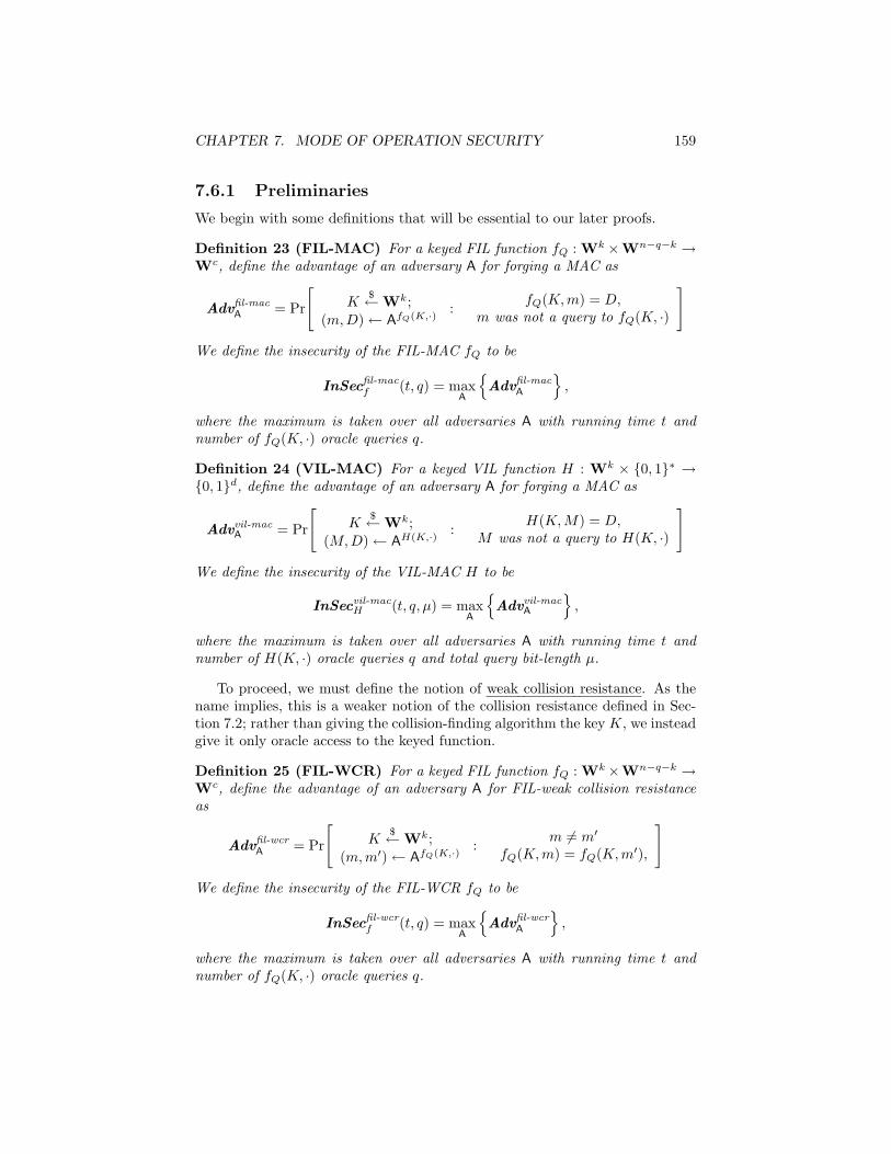
CHAPTER 7. MODE OF OPERATION SECURITY 159
7.6.1 Preliminaries
We begin with some definitions that will be essential to our later proofs.
Definition 23 (FIL-MAC) For a keyed FIL function fQ : Wk ×Wn−q−k →Wc, define the advantage of an adversary A for forging a MAC as
Advfil-macA = Pr
[K
$←Wk;(m,D)← AfQ(K,·) :
fQ(K,m) = D,m was not a query to fQ(K, ·)
]We define the insecurity of the FIL-MAC fQ to be
InSecfil-macf (t, q) = max
A
{Advfil-mac
A
},
where the maximum is taken over all adversaries A with running time t andnumber of fQ(K, ·) oracle queries q.
Definition 24 (VIL-MAC) For a keyed VIL function H : Wk × {0, 1}∗ →{0, 1}d, define the advantage of an adversary A for forging a MAC as
Advvil-macA = Pr
[K
$←Wk;(M,D)← AH(K,·) :
H(K,M) = D,M was not a query to H(K, ·)
]We define the insecurity of the VIL-MAC H to be
InSecvil-macH (t, q, µ) = max
A
{Advvil-mac
A
},
where the maximum is taken over all adversaries A with running time t andnumber of H(K, ·) oracle queries q and total query bit-length µ.
To proceed, we must define the notion of weak collision resistance. As thename implies, this is a weaker notion of the collision resistance defined in Sec-tion 7.2; rather than giving the collision-finding algorithm the key K, we insteadgive it only oracle access to the keyed function.
Definition 25 (FIL-WCR) For a keyed FIL function fQ : Wk×Wn−q−k →Wc, define the advantage of an adversary A for FIL-weak collision resistanceas
Advfil-wcrA = Pr
[K
$←Wk;(m,m′)← AfQ(K,·) :
m 6= m′
fQ(K,m) = fQ(K,m′),
]We define the insecurity of the FIL-WCR fQ to be
InSecfil-wcrf (t, q) = max
A
{Advfil-wcr
A
},
where the maximum is taken over all adversaries A with running time t andnumber of fQ(K, ·) oracle queries q.
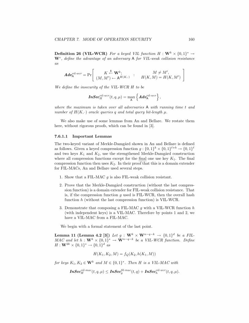
CHAPTER 7. MODE OF OPERATION SECURITY 160
Definition 26 (VIL-WCR) For a keyed VIL function H : Wk × {0, 1}∗ →Wc, define the advantage of an adversary A for VIL-weak collision resistanceas
Advvil-wcrA = Pr
[K
$←Wk;(M,M ′)← AH(K,·) :
M 6= M ′,H(K,M) = H(K,M ′)
]
We define the insecurity of the VIL-WCR H to be
InSecvil-wcrH (t, q, µ) = max
A
{Advvil-wcr
A
},
where the maximum is taken over all adversaries A with running time t andnumber of H(K, ·) oracle queries q and total query bit-length µ.
We also make use of some lemmas from An and Bellare. We restate themhere, without rigorous proofs, which can be found in [3].
7.6.1.1 Important Lemmas
The two-keyed variant of Merkle-Damgard shown in An and Bellare is definedas follows. Given a keyed compression function g : {0, 1}k × {0, 1}`+b → {0, 1}`and two keys K1 and K2, use the strengthened Merkle-Damgard constructionwhere all compression functions except for the final one use key K1. The finalcompression function then uses K2. In their proof that this is a domain extenderfor FIL-MACs, An and Bellare used several steps.
1. Show that a FIL-MAC g is also FIL-weak collision resistant.
2. Prove that the Merkle-Damgard construction (without the last compres-sion function) is a domain extender for FIL-weak collision resistance. Thatis, if the compression function g used is FIL-WCR, then the overall hashfunction h (without the last compression function) is VIL-WCR.
3. Demonstrate that composing a FIL-MAC g with a VIL-WCR function h(with independent keys) is a VIL-MAC. Therefore by points 1 and 2, wehave a VIL-MAC from a FIL-MAC.
We begin with a formal statement of the last point.
Lemma 11 (Lemma 4.2 [3]) Let g : Wk ×Wn−q−k → {0, 1}d be a FIL-MAC and let h : Wk × {0, 1}∗ → Wn−q−k be a VIL-WCR function. DefineH : W2k × {0, 1}∗ → {0, 1}d as
H(K1,K2,M) = fQ(K2, h(K1,M))
for keys K1,K2 ∈Wk and M ∈ {0, 1}∗. Then H is a VIL-MAC with
InSecvil-macH (t, q, µ) ≤ InSecfil-mac
g (t, q) + InSecvil-wcrh (t, q, µ).
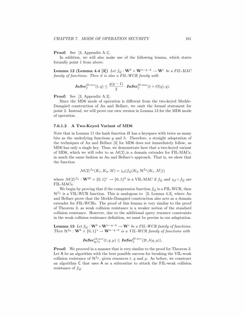
CHAPTER 7. MODE OF OPERATION SECURITY 161
Proof: See [3, Appendix A.1].In addition, we will also make use of the following lemma, which states
formally point 1 from above.
Lemma 12 (Lemma 4.4 [3]) Let fQ : Wk ×Wn−q−k →Wc be a FIL-MACfamily of functions. Then it is also a FIL-WCR family with
InSecfil-wcrf (t, q) ≤ q(q − 1)
2· InSecfil-mac
f (t+O(q), q).
Proof: See [3, Appendix A.3].Since the MD6 mode of operation is different from the two-keyed Merkle-
Damgard construction of An and Bellare, we omit the formal statement forpoint 2. Instead, we will prove our own version in Lemma 13 for the MD6 modeof operation.
7.6.1.2 A Two-Keyed Variant of MD6
Note that in Lemma 11 the hash function H has a keyspace with twice as manybits as the underlying functions g and h. Therefore, a straight adaptation ofthe techniques of An and Bellare [3] for MD6 does not immediately follow, asMD6 has only a single key. Thus, we demonstrate here that a two-keyed variantof MD6, which we will refer to as M〈2〉,is a domain extender for FIL-MACs,in much the same fashion as An and Bellare’s approach. That is, we show thatthe function
M〈2〉fQ(K1,K2,M) = χd(fQ(K2,HfQ(K1,M)))
where M〈2〉fQ : W2k × {0, 1}∗ → {0, 1}d is a VIL-MAC if fQ and χd ◦ fQ areFIL-MACs.
We begin by proving that if the compression function fQ is a FIL-WCR, thenHfQ is a VIL-WCR function. This is analogous to [3, Lemma 4.3], where Anand Bellare prove that the Merkle-Damgard construction also acts as a domainextender for FIL-WCRs. The proof of this lemma is very similar to the proofof Theorem 3, as weak collision resistance is a weaker notion of the standardcollision resistance. However, due to the additional query resource constraintsin the weak collision resistance definition, we must be precise in our adaptation.
Lemma 13 Let fQ : Wk×Wn−q−k →Wc be a FIL-WCR family of functions.Then HfQ : Wk × {0, 1}∗ →Wn−q−k is a VIL-WCR family of functions with
InSecvil-wcrHfQ (t, q, µ) ≤ InSecfil-wcr
f (2t, δ(q, µ)).
Proof: We proceed in a manner that is very similar to the proof for Theorem 3.Let A be an algorithm with the best possible success for breaking the VIL-weakcollision resistance of HfQ , given resources t, q and µ. As before, we constructan algorithm C that uses A as a subroutine to attack the FIL-weak collisionresistance of fQ.
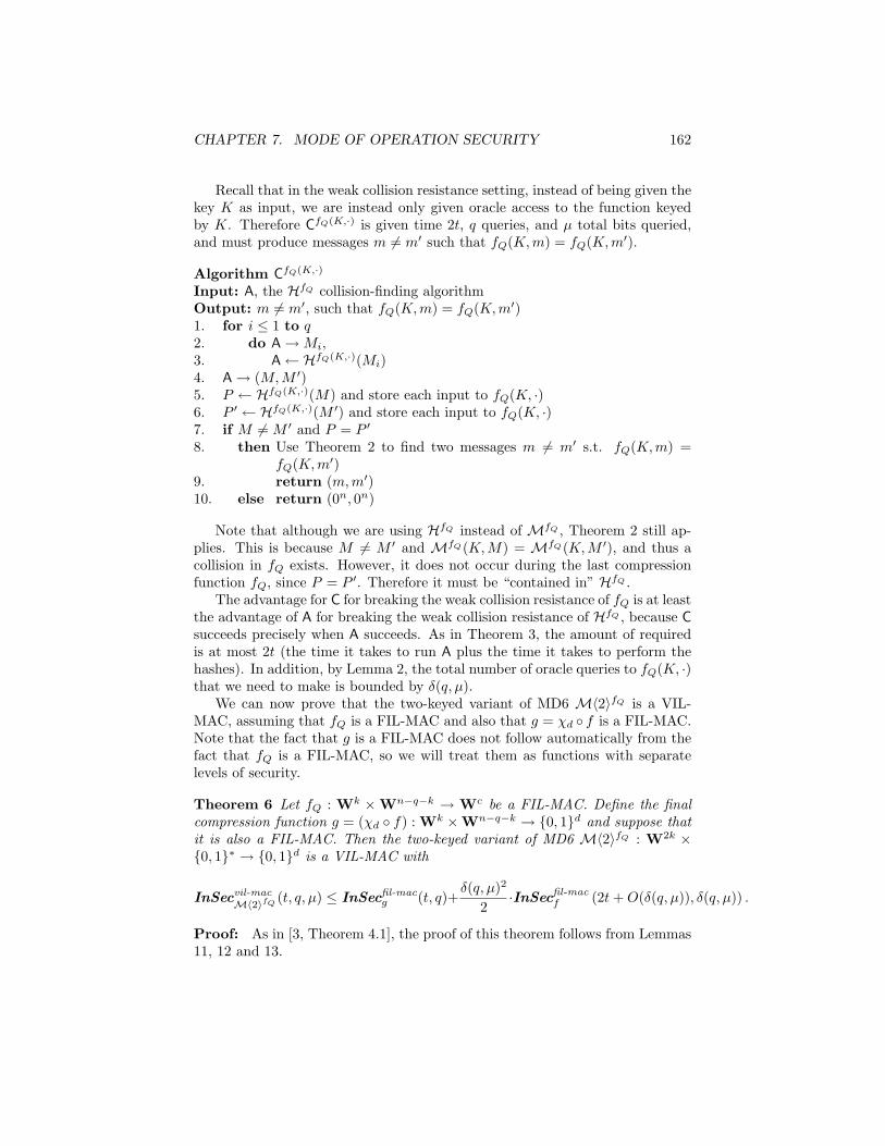
CHAPTER 7. MODE OF OPERATION SECURITY 162
Recall that in the weak collision resistance setting, instead of being given thekey K as input, we are instead only given oracle access to the function keyedby K. Therefore CfQ(K,·) is given time 2t, q queries, and µ total bits queried,and must produce messages m 6= m′ such that fQ(K,m) = fQ(K,m′).
Algorithm CfQ(K,·)
Input: A, the HfQ collision-finding algorithmOutput: m 6= m′, such that fQ(K,m) = fQ(K,m′)1. for i ≤ 1 to q2. do A→Mi,3. A← HfQ(K,·)(Mi)4. A→ (M,M ′)5. P ← HfQ(K,·)(M) and store each input to fQ(K, ·)6. P ′ ← HfQ(K,·)(M ′) and store each input to fQ(K, ·)7. if M 6= M ′ and P = P ′
8. then Use Theorem 2 to find two messages m 6= m′ s.t. fQ(K,m) =fQ(K,m′)
9. return (m,m′)10. else return (0n, 0n)
Note that although we are using HfQ instead of MfQ , Theorem 2 still ap-plies. This is because M 6= M ′ and MfQ(K,M) = MfQ(K,M ′), and thus acollision in fQ exists. However, it does not occur during the last compressionfunction fQ, since P = P ′. Therefore it must be “contained in” HfQ .
The advantage for C for breaking the weak collision resistance of fQ is at leastthe advantage of A for breaking the weak collision resistance of HfQ , because Csucceeds precisely when A succeeds. As in Theorem 3, the amount of requiredis at most 2t (the time it takes to run A plus the time it takes to perform thehashes). In addition, by Lemma 2, the total number of oracle queries to fQ(K, ·)that we need to make is bounded by δ(q, µ).
We can now prove that the two-keyed variant of MD6 M〈2〉fQ is a VIL-MAC, assuming that fQ is a FIL-MAC and also that g = χd ◦ f is a FIL-MAC.Note that the fact that g is a FIL-MAC does not follow automatically from thefact that fQ is a FIL-MAC, so we will treat them as functions with separatelevels of security.
Theorem 6 Let fQ : Wk ×Wn−q−k → Wc be a FIL-MAC. Define the finalcompression function g = (χd ◦ f) : Wk ×Wn−q−k → {0, 1}d and suppose thatit is also a FIL-MAC. Then the two-keyed variant of MD6 M〈2〉fQ : W2k ×{0, 1}∗ → {0, 1}d is a VIL-MAC with
InSecvil-macM〈2〉fQ (t, q, µ) ≤ InSecfil-mac
g (t, q)+δ(q, µ)2
2·InSecfil-mac
f (2t+O(δ(q, µ)), δ(q, µ)) .
Proof: As in [3, Theorem 4.1], the proof of this theorem follows from Lemmas11, 12 and 13.
CHAPTER 7. MODE OF OPERATION SECURITY 163
InSecvil-macM〈2〉fQ (t, q, µ) ≤ InSecfil-mac
g (t, q) + InSecvil-wcrHfQ (t, q, µ)
≤ InSecfil-macg (t, q) + InSecfil-wcr
f (2t, δ(q, µ))
≤ InSecfil-macg (t, q) +
δ(q, µ)2
2· InSecfil-mac
f (2t+O(δ(q, µ)), δ(q, µ))
7.6.2 MD6 as a Domain Extender for FIL-MACs
It seems somewhat artificial to double the number of bits in the keyspace ofMD6 simply to prove that it acts as a domain extender for FIL-MACs. Ideally,we would like to prove that it has this property as is, while still only makingthe assumption that the underlying compression functions fQ and g are FIL-MACs. Unfortunately, at the moment we do not know how to prove this directly(although we have no counterexample for this property). Thus, in order to provethis statement for the standard version of MD6, we will make use of they key-blinding assumption defined in Section 6.8.
Recall that the key-blinding assumption states that the flag bit z effectively“blinds” the key values. That is, given oracle access to two functions:
f0Q(·) = fQ(z = 0,K = κ0, ·)f1Q(·) = fQ(z = 1,K = κ1, ·)
then we should not be able to guess whether κ0 = κ1 or not with any significantadvantage. Recalling Definition 2:
Definition 27 (Key-Blinding Assumption) Let D be a distinguisher givenoracle access to two functions f0
Q and f1Q that map Wk ×Wn−q−k−1 → Wc.
We define its advantage as follows.
AdvblindD,fQ
(t, q) =
∣∣∣∣∣ Pr
[κ0
$←Wk;κ1$←Wk; b $← {0, 1};
a← DfQ(z=0,κ0,·),fQ(z=1,κb,·): a = b
]− 1
2
∣∣∣∣∣The goal of D is to try to determine the value of b, i.e. whether f0
Q and f1Q use
the same key or not. We can define the overall insecurity of the key-blindingproperty of fQ to be
InSecblindfQ
(t, q) = maxD
{Advblind
D,fQ(t, q)
},
where D is given resource constraints of (t, q).
With this assumption, we now prove that the single-keyed version of MD6acts as a domain extender for FIL-MACs (with the key-blinding assumption).The essential concept here is that by the key-blinding property of fQ, MfQ
behaves almost exactly like M〈2〉fQ to any algorithm given only oracle accessto MfQ .
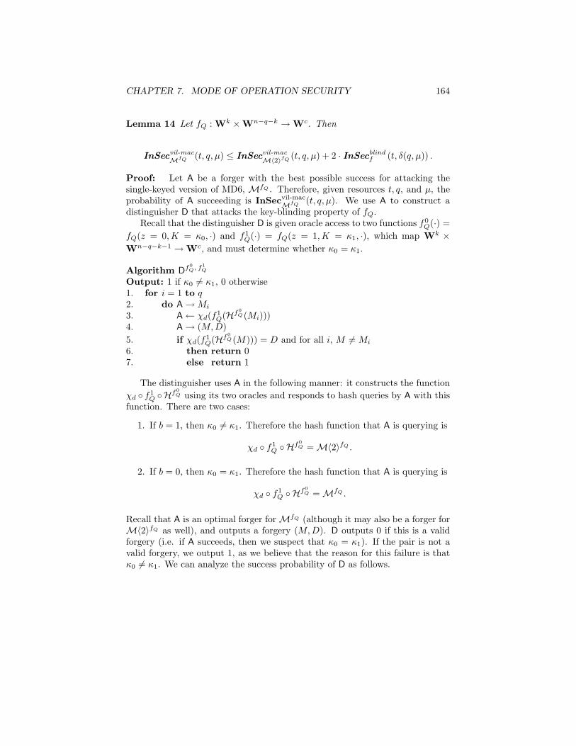
CHAPTER 7. MODE OF OPERATION SECURITY 164
Lemma 14 Let fQ : Wk ×Wn−q−k →Wc. Then
InSecvil-macMfQ (t, q, µ) ≤ InSecvil-mac
M〈2〉fQ (t, q, µ) + 2 · InSecblindf (t, δ(q, µ)) .
Proof: Let A be a forger with the best possible success for attacking thesingle-keyed version of MD6, MfQ . Therefore, given resources t, q, and µ, theprobability of A succeeding is InSecvil-mac
MfQ (t, q, µ). We use A to construct adistinguisher D that attacks the key-blinding property of fQ.
Recall that the distinguisher D is given oracle access to two functions f0Q(·) =
fQ(z = 0,K = κ0, ·) and f1Q(·) = fQ(z = 1,K = κ1, ·), which map Wk ×
Wn−q−k−1 →Wc, and must determine whether κ0 = κ1.
Algorithm Df0Q, f
1Q
Output: 1 if κ0 6= κ1, 0 otherwise1. for i = 1 to q2. do A→Mi
3. A← χd(f1Q(Hf
0Q(Mi)))
4. A→ (M,D)5. if χd(f1
Q(Hf0Q(M))) = D and for all i, M 6= Mi
6. then return 07. else return 1
The distinguisher uses A in the following manner: it constructs the functionχd ◦ f1
Q ◦Hf0Q using its two oracles and responds to hash queries by A with this
function. There are two cases:
1. If b = 1, then κ0 6= κ1. Therefore the hash function that A is querying is
χd ◦ f1Q ◦ Hf
0Q =M〈2〉fQ .
2. If b = 0, then κ0 = κ1. Therefore the hash function that A is querying is
χd ◦ f1Q ◦ Hf
0Q =MfQ .
Recall that A is an optimal forger forMfQ (although it may also be a forger forM〈2〉fQ as well), and outputs a forgery (M,D). D outputs 0 if this is a validforgery (i.e. if A succeeds, then we suspect that κ0 = κ1). If the pair is not avalid forgery, we output 1, as we believe that the reason for this failure is thatκ0 6= κ1. We can analyze the success probability of D as follows.
CHAPTER 7. MODE OF OPERATION SECURITY 165
Pr[D succeeds] = Pr[b = 1] · Pr[DfQ(z=0,K=κ0,·), fQ(z=1,K=κb,·) → 1 | b = 1
]+ Pr[b = 0] · Pr
[DfQ(z=0,K=κ0,·), fQ(z=1,K=κb,·) → 0 | b = 0
]=
12· Pr[A fails to forge M〈2〉fQ
]+
12· Pr[A successfully forges MfQ
]≥ 1
2·(
1− InSecvil-macM〈2〉fQ (t, q, µ)
)+
12· InSecvil-mac
MfQ (t, q, µ)
(7.7)
=12
+InSecvil-mac
MfQ (t, q, µ)− InSecvil-macM〈2〉fQ (t, q, µ)
2
For Inequality (7.7), note that A could potentially succeed as a forger forM〈2〉fQ . However, its advantage is bounded, as Advvil-mac
A,M〈2〉fQ (t, q, µ) ≤ InSecvil-macM〈2〉fQ (t, q, µ),
whereby we derive the inequality. Therefore,
AdvblindD,fQ
(t, δ(q, µ)) =∣∣∣∣Pr[D succeeds]− 1
2
∣∣∣∣≥
∣∣∣InSecvil-macMfQ (t, q, µ)− InSecvil-mac
M〈2〉fQ (t, q, µ)∣∣∣
2
InSecblindfQ
(t, δ(q, µ)) ≥
∣∣∣InSecvil-macMfQ (t, q, µ)− InSecvil-mac
M〈2〉fQ (t, q, µ)∣∣∣
2
In particular, this implies
InSecvil-macMfQ (t, q, µ) ≤ InSecvil-mac
M〈2〉fQ (t, q, µ) + 2 · InSecblindfQ
(t, δ(q, µ))
We now conclude by applying the above lemma to derive a bound on theinsecurity of MfQ .
Theorem 7 Let fQ : Wk ×Wn−q−k →Wc be a FIL-MAC and suppose thatit has the key-blinding property. Define g = (χd ◦ f) : Wk ×Wn−q−k → {0, 1}dand suppose that it is also a FIL-MAC. Then MfQ : Wk × {0, 1}∗ → {0, 1}d isa VIL-MAC with
InSecvil-macMfQ (t, q, µ) ≤ δ(q, µ)2
2· InSecfil-mac
fQ(2t+O(δ(q, µ)), δ(q, µ)) +
InSecfil-macg (t, q) + 2 · InSecblind
fQ(t, δ(q, µ)) .
Proof: This follows directly by the application of Theorem 6 and Lemma 14.Therefore we have shown that the MD6 mode of operation MfQ acts as a
domain extender for FIL-MACs, assuming that both fQ and g are FIL-MACs
CHAPTER 7. MODE OF OPERATION SECURITY 166
and that fQ has the key-blinding property. Unfortunately we needed to makean additional assumption about the compression function fQ, and as such thisis not a true “domain extension” result. However, at the moment we know ofno other way to prove that MD6 has this property, without making additionalassumptions.
7.7 Indifferentiability from Random Oracle
In this section, we present a proof that the MD6 mode of operation is indiffer-entiable from a random oracle assuming that the MD6 compression function isa random oracle. Let fQ : Wn−q → Wc be the reduced compression functiondefined in Section 2.4, and let MfQ be the MD6 mode of operation applied tofQ. Section 6.1.2 presents a proof that the reduced MD6 compression functionfQ is indifferentiable from a random oracle under the assumption that fQ isbased on a random permutation. Thus, in this section, we will assume that fQis a random oracle.
We use Definition 1 from Section 6.1.2 for the notion of indifferentiability,again relying on the framework of Maurer et al. [59] and the approach of Coronet al. [31], but this time to analyze the MD6 mode of operation rather than theMD6 compression function.
Theorem 8 If fQ : Wn−q →Wc is a random oracle, thenMfQ is (t, qF , qS , ε)-indifferentiable from a random oracle F : {0, 1}∗ → {0, 1}d, with ε = 2q2
t /2cw
and t = O(q2S), for any qF and qS such that the total number of compression
function calls from the mode of operation queries and the compression functionqueries of the distinguisher is at most qt.
Proof: Fix a distinguisher D that makes exactly qS compression functionqueries and generates exactly qt compression function calls from its mode ofoperation queries and its compression function queries. We will assume that allof D’s compression function queries are of length (n− q) words.
Let γa(X) denote a function that truncates its input X by dropping its lasta bits.
We will define a simulator S with access to a random oracle F : {0, 1}∗ →{0, 1}d as follows.
Upon receiving a compression function query x∗, S will use the algorithmdescribed below to decide to either answer with its own fresh random string orconsult F and return an answer based on the answer of F . (However, no matterwhat, S will repeat the same answer if the query x∗ has been seen before.) Thisdecision is made as follows: S consults F on those queries x∗ that correspondto the final compression function call in an MD6 computation for which allintermediate compression function calls have already been queried to S. Wewill call such compression function queries “final”. For all other queries x∗, Sanswers with its own fresh random string.
More formally, S maintains a table T , initially empty, containing the pairs(x,C) ∈Wn−q×Wc such that S has answered C in response to a query x. For
CHAPTER 7. MODE OF OPERATION SECURITY 167
each pair (x,C), S also maintains the most recent time τ that it answered C inresponse to the query x. For simplicity, in the description of S we will omit therecording of these times.
Upon receiving a compression function query x∗, S executes the followingalgorithm.
1. Search T for a pair (x∗, C∗). If such a pair is found, return C∗ as theanswer to the query.
2. Parse x∗ into K∗, `∗, i∗, r∗, L∗, z∗, p∗, keylen∗, d∗, B∗.
3. If any of the following conditions is true, choose a fresh random stringC∗ ∈Wc and return C∗ as the answer to the query:
(a) z∗ 6= 1
(b) `∗ > L∗ + 1
(c) The last p∗ bits of B∗ are not all 0.
(d) 0 ≤ `∗ ≤ L and i∗ 6= 0
(e) d∗ 6= d
4. The simulator now decides whether x∗ is a final query by searching fora legitimate way to build a complete MD6 computation from previouscompression function queries to S, with x∗ as the input to the final com-pression function call.
If 0 ≤ `∗ ≤ L (only the PAR operation is used), let B`∗,0 = B∗, j`∗ = 0,and p`∗,0 = p∗. Search T for a sequence of pairs (x`,i, C`,i) satisfying thefollowing condition:
(a) For ` = 1, 2, . . . , `∗ − 1,B`+1,0||B`+1,1|| . . . ||B`+1,j`+1 = C`,0||C`,1|| . . . ||C`,j` ||0
p`+1,j`+1 and
• For i = 0, 1, . . . , j`,x`,i = K∗||U`,i||r∗||L∗||0||p`,i||keylen∗||d∗||B`,i, where U`,i = ` ·256 + i, p`,i = 0 for i = 0, 1, . . . , j` − 1, and the last p`,j` bits ofB`,i are 0.
If no satisfying sequence is found, choose a fresh random string C∗ ∈Wc.Insert (x∗, C∗) into T and return C∗ as the answer to the query.
If a satisfying sequence is found, let M∗ = B1,0||B1,1|| . . . ||γp1,j1(B1,j1).(Recall that γa(X) denotes a function that truncates its input X by drop-ping its last a bits.)
If multiple satisfying sequences are found, yielding different values of M∗,choose the one which comes last chronologically, in the following sense. Foreach satisfying sequence, sort the compression function queries by nodeidentifier U . Choose the sequence with the most recent time τ recorded forthe first compression function query (` = 1, i = 0). If there are multiple
CHAPTER 7. MODE OF OPERATION SECURITY 168
such sequences, choose the sequence with the most recent time τ for thenext compression function query (` = 1, i = 1), and so on, until a uniqueM∗ is obtained.
Query M∗ to F , and let F (M∗) ∈ {0, 1}d denote F ’s answer. Pad F (M∗)to the full length of the compression function output by choosing a randomstring C ′ ∈ {0, 1}cw−d and letting C∗ = C ′||F (M∗). Insert (x∗, C∗) intoT and return C∗ as the answer to the query.
5. If `∗ = L∗ + 1 (the SEQ operation is used), write B∗ as C`∗,i∗−1||B`∗,i∗where C`∗,i∗−1 ∈Wc and B`∗,i∗ ∈Wb−c. Search T for a sequence of pairs(x`∗,i, C`∗,i) such that:
(a) For i = 0, 1, . . . , i∗,x`∗,i = K∗||U`∗,i||r∗||L∗||0||0||keylen∗||d∗||C`∗,i−1||B`∗,i, where U`∗,i =`∗ · 256 + i and C`∗,−1 is the c-word zero vector.
If no satisfying sequence is found, choose a fresh random string C∗ ∈Wc.Insert (x∗, C∗) into T and return C∗ as the answer to the query.
Otherwise, for each satisfying sequence, let j`∗ = i∗ and p`∗,i∗ = p∗, andsearch T for a sequence of pairs (x`,i, C`,i) satisfying the condition givenabove, for the PAR operation, in item 4a.
If no satisfying sequence is found, choose a fresh random string C∗ ∈Wc.Insert (x∗, C∗) into T and return C∗ as the answer to the query.
If a satisfying sequence is found, let M∗ = B1,0||B1,1|| . . . ||γp1,j1(B1,j1).If multiple satisfying sequences are found, yielding different values of M∗,choose the one which comes last chronologically (as described previously).Query M∗ to F , and let F (M∗) ∈ {0, 1}d denote F ’s answer. Pad F (M∗)to the full length of the compression function output by choosing a randomstring C ′ ∈ {0, 1}cw−d and letting C∗ = C ′||F (M∗). Insert (x∗, C∗) intoT and return C∗ as the answer to the query.
This completes the description of the simulator S. Notice that if the simu-lator is queried on the final compression function call in the computation of theMD6 hash of a message after all intermediate compression function calls havealready been queried to it, the simulator will find an M∗ and determine thequery to be a final query.
Using a data structure such as a linked list to maintain T in sorted order,S takes time at most O(qS) to respond to each of the qS compression functionqueries. Therefore, the running time of the simulator is O(q2
S).To prove the indifferentiability of the MD6 mode of operation, we consider
any distinguisher D making exactly qS compression function queries and gen-erating exactly qt compression function calls from its MD6 queries and its com-pression function queries. We consider a sequence of games, G0 through G4. Foreach game Gi, let pi denote the probability that D outputs 1 in Gi. We startwith the “ideal” game and end with the “real” game. We show that between
CHAPTER 7. MODE OF OPERATION SECURITY 169
consecutive games, the view of the distinguisher cannot differ with more thannegligible probability.
Game G0. This is the interaction of D with the random oracle F and thepolynomial time simulator S defined above.
Game G1. In game G1, D interacts with F and a modified simulator S′.At the start of the game, S′ uses its random coins to specify a random oracleOS : Wn−q →Wc. The behavior of the new simulator S′ is identical to that ofS, except that wherever S uses a fresh random string C∗ ∈Wc to answer a queryx∗, S′ uses OS(x∗). Wherever S uses a fresh random string C ′ ∈ {0, 1}cw−d inconstructing the answer to a query x∗, S′ uses the first cw − d bits of OS(x∗).In other words, in G1, S generates its random bits in a lazy manner, whereasin G2, S′ generates its random bits by calling a random oracle OS (specified bythe random coins of S′). In both games, the simulator produces a fresh randomstring in exactly the same cases. Clearly, the view of the distinguisher is thesame in G1 and in G0, so p1 = p0.
Game G2. In G2, D interacts with a dummy relay algorithm R0, insteadof with F . The relay algorithm R0 has oracle access to F , and upon receivinga hash function query, it forwards the query to F and forwards F ’s response toD. Clearly, the view of D is unchanged from G0, so p2 = p1.
Game G3. In G3, we modify the relay algorithm. The new relay algorithmR1 does not query F . Instead, R1 computes the MD6 mode of operation on itsinput, querying the simulator S′ for each call to the compression function fQ.
In order to argue that the view of D differs between G2 and G3 with onlynegligible probability, we first define some “bad” events. We then argue that,as long as no bad events occur, the view of D is identical in games G2 and G3.
For a compression function query xj , suppose xj parses into Kj , `j , ij , rj ,Lj , zj , pj , keylenj , dj , Bj . We define three types of bad events that can occur ineither game.
Type 1 A Type 1 event occurs when the outputs of S′ on two different inputsare equal. Specifically, a Type 1 event occurs when S′ inserts a pair (x2, C)into T when there is already a pair (x1, C) in T such that x1 6= x2.
Type 2 A Type 2 event occurs when the output of S′ on a query x2 is suchthat a previous query x1 “depends” on the answer to x2. Specifically, aType 2 event occurs when S′ inserts a pair (x2, C2) into T when there isalready a pair (x1, C1) in T such that L1 = L2 and one of the followingtwo conditions is true:
• 0 ≤ `1 ≤ L1, `1 = `2 + 1, i1 = bi2 · c/bc, and C2 is the kth c-wordchunk of B1, where k = i2 mod b/c.
• `1 = `2 = L1 + 1, i1 = i2 + 1, and C2 is the first chunk of B1.
Type 3 A Type 3 event occurs when S′ receives a query x2 from D that “de-pends” on an answer which was given by S′ only to the relay algorithm,
CHAPTER 7. MODE OF OPERATION SECURITY 170
never to D. Specifically, a Type 3 event occurs when S′ receives a queryx2 from D when there is already a pair (x1, C1) in T such that L1 = L2
and one of the following two conditions is true:
• 0 ≤ `2 ≤ L1, `2 = `1 + 1, i2 = bi1 · c/bc, and C1 is the kth chunk ofB2, where k = i1 mod b/c, and C1 has been given as the answer toa query x1 only to R1, never to D.
• `1 = `2 = L1 + 1, i2 = i1 + 1, and C1 is the first chunk of B2, and C1
has been given as the answer to a query x1 only to R1, never to D.
We argue below that if none of these bad events occur, then the view of Din G2 and G3 is the same.
Lemma 15 For fixed coins of F , S′, and D, if no “bad” events occur in gameG3, then the view of D is identical in games G2 and G3.
Proof: Fix the random coins of F , S′, and D. Assume no “bad” events oc-curred. We show by induction that the observable values (the responses ofR0/R1 and S′) are identical in games G2 and G3. (As long as the observablevalues are the same, D will make the same queries in both games.)
Suppose that the observable values have been the same so far. The nextquery by D is either to MD6 or to the compression function.
Mode of Operation Query. Consider a query M∗ toMfQ . In game G2, R0
always returns F (M∗). In game G3, R1 returns F (M∗) as long as on R1’s finalcompression function query (call this x∗) to S′, S′ queries F on M∗, or S′ hasalready seen the query x∗ and queried F on M∗ the first time it was queriedon x∗. If S′ has not already seen the query x∗, S′ will return F (M∗), since inthe case that it finds multiple values of M which could have generated x∗ as itsfinal compression function call, S′ will choose the M for which the intermediatecompression function calls occurred the most recently. Therefore, the only waythat R1’s answer can differ from R0’s answer is if S′ has already seen the queryx∗ and did not query F on M∗ the first time it saw the query (call that timeτ).
In this case, when S′ was originally queried on x∗ at time τ , it must haveeither (a) found no M or (b) found an M 6= M∗ which could have generated thequery as its final compression function call. Assume (a), i.e., S′ found no suchM . Consider R1’s most recent query to S′ before x∗. (Recall that R1 computesthe mode of operation by making the compression function queries in order.)That query must have also been seen by S′ before time τ . Otherwise, a Type2 event occurred in G3 because the output of that query matched a chunk ofthe query at time τ . Now consider R1’s next most recent query. Again, by thesame reasoning, it was also seen before time τ . By induction, all of the queriesR1 makes to S′ on the message M∗ must have been seen before time τ , whichmeans that case (a) is impossible.
Now consider case (b). We have already argued that all of the queries R1
makes to S′ on the message M∗ must have been seen before time τ . Therefore,
CHAPTER 7. MODE OF OPERATION SECURITY 171
when S′ was originally queried on x∗ at time τ , it must have found both M∗ andan M 6= M∗ which could have generated x∗ as its final compression functioncall. Consider the b-word data input B∗ of x∗. For each of the c-word chunksof B∗, either there was a unique pair in T at time τ with that chunk as theresponse, or there were multiple such pairs. If there were multiple such pairs,then a Type 1 event occurred. Otherwise, consider of all of the b-word datainputs of the compression function queries made by R1 on the message M∗, atthe next lower level. By induction, a Type 1 event must have occurred at sometime; otherwise, S′ would only have found one M (equal to M∗) that could havegenerated the final compression query. Therefore, case (b) is also impossible.
Thus, given that the values observable to D have been the same so far, ifthe next query is to the mode of operation, the next observable value will alsobe the same in games G2 and G3.
Compression Function Query. Now consider the case that the next queryby D is a compression function query x∗. In both games, the answer will beequal to OS(x∗), unless x∗ is (or has previously been) determined to be thefinal query for some message M , in which case it will be equal to C ′||F (M)where C ′ = γd(OS(x∗)). Thus, there are three possible reasons for the answersin the two games to be different: (a) the answer is equal to C ′||F (M) in G2 butOS(x∗) in G3; (b) the answer is equal to C ′||F (M) in G3 but OS(x∗) in G2; or(c) the answer is equal to C ′||F (M) in G2 but C ′||F (M ′) in G3 for M 6= M ′.
Consider case (a). In G3, S′ answers with OS(x∗) because either (a.1) S′
already answered a query on x∗ before or (a.2) S′ cannot find a sequence ofqueries that leads to M for which x∗ is the final query. Case (a.1) is not possiblebecause for S′ to have the seen the query x∗ before in G3 but not in G2 meansthat the query came from R1, and if a final query comes from R1 in G3, thenR1 has asked all of the intermediate queries, and therefore it will be answeredby C ′||F (M). Case (a.2) is not possible because the queries S′ has received inG2 are a subset of the queries S′ has received in G3 (in G3, S′ has received allthe same queries as in G2 from D, as well as queries from R1). Therefore, if S′
finds an M in G2, it will also find some M in G3.In case (b), S′ finds an M in G3 but not in G2. Then at least one query
in the sequence used to construct M came from R1 but not from D. But thefinal query (namely, x∗) came from D. By induction, a Type 3 event must haveoccurred, i.e., a chunk of one of D’s compression function queries matched acompression function output that was answered to R1 but never seen by D.Therefore, case (b) is impossible.
In case (c), S′ finds M in G2 and M ′ in G3. But since the queries to S′ inG2 are a subset of the queries to S′ in G3, in G3 S
′ must find both M and M ′.Then, again, a Type 1 event must have occurred somewhere in the computation,making case (c) also impossible.
Thus, given that the values observable to D have been the same so far, if thenext query is to the compression function, the next observable value will alsobe the same in games G2 and G3.
CHAPTER 7. MODE OF OPERATION SECURITY 172
Thus, conditioned on there being no occurrences of bad events in G3, theview of D is the same in games G2 and G3. This completes the proof ofLemma 15
We now bound the probability of bad events in G3. Let Pr[Type i] denotethe probability that a Type i event ever occurs during the run of the simulator.Let Pr[Bad] = Pr[Type 1] + Pr[Type 2] + Pr[Type 3] denote the probability ofa bad event ever occurring.
A Type 1 event corresponds to a collision between two random c-word stringsamong at most qt compression function queries. Note that even though S′
sometimes consults F for d bits of the random c-word output, these d randombits are fresh because on different queries to S′, S′ will make different queriesto F (if it queries F at all). We can bound the probability of a Type 1 eventusing the birthday bound: Pr[Type 1] ≤ q2
t /2cw+1.
A Type 2 event corresponds to a collision between a random c-word stringand a chunk of one of the previous queries to the compression function. Foreach of the qt compression function queries x, in each of the previous compres-sion function queries, there is at most one c-word chunk with a matching nodeidentifier with which x could collide to cause a Type 2 event. Therefore, we canagain bound the probability using the birthday bound: Pr[Type 2] ≤ q2
t /2cw+1.
A Type 3 event corresponds to a collision between a random c-word stringthat is not seen by D and a chunk of one of D’s compression function queries.The probability of D “guessing” one of these hidden outputs is 1/2cw. Thereare at most (qt − qS) hidden outputs to guess, and D has at most qt guesses.Therefore, Pr[Type 3] ≤ (qt(qt − qS))/2cw.
Summing together, we get Pr[Bad] ≤ (q2t + qt(qt − qS))/2cw ≤ 2q2
t /2cw.
Therefore, the probability ofD distinguishing between gamesG2 andG3 is atmost the probability of a bad event occurring, so |p3 − p2| ≤ Pr[Bad] ≤ 2q2
t /2cw.
Game G4. This is the final game. In G4, the relay algorithm R1 remainsunchanged but the simulator no longer consults F . Instead, the new simulator,S1, always responds to a new query x∗ with OS(x∗). Thus, R1 computes themode of operation applied to the random oracle OS(x∗).
To see that the view of the distinguisher is unchanged from G3, consider aquery x∗ (from either D or R1) to S1. If the query has been seen before, S1
repeats the answer it gave the first time it was asked the query. If it is a newquery, then in G4, S1 responds with the fresh random c-word string OS(x∗).In G3, S′ either responded with the fresh random c-word string OS(x∗) or thefresh random c-word string obtained by concatenating the first (cw− d) bits ofOS(x∗) with a fresh random d-bit string obtained from F . The only way thatthe random d-bit string from F could not be fresh is if S′ already consulted Fon the same message before, but this would mean that the query x∗ was seenbefore. Thus, the view of D is unchanged from G3 to G4, and p4 = p3.
Summing over all the games, the total advantage of D in distinguishingbetween G0 and G4 is at most the claimed 2q2
t /2cw. This completes the proof
CHAPTER 7. MODE OF OPERATION SECURITY 173
of Theorem 8.
7.8 Multi-Collision Attacks
In this section we again briefly discuss the class of recent “multi-collision” at-tacks studied by Joux [46], Nandi et al. [68, 69], Hoch et al. [44], and Yu etal. [98]. (Our previous discussion was in Section 3.8.)
These attacks leverage a compression function that is known not to becollision-resistant to obtain collisions in hash function modes of operation thatare intended to compensate for or mitigate such weaknesses. Often, a surprisingnumber of such collisions can be obtained, allowing further birthday attacks tobe mounted.
MD6 adopts the “wide-pipe” strategy proposed by Lucks [54, 55]: all inter-mediate chaining variables in MD6 are 1024 bits in length, making collisions ofthe compression function extremely unlikely.
Thus, unless there is some unforeseen defect in the MD6 compression func-tion, such “multi-collision” attacks will not be effective against MD6.
7.9 Length-Extension Attacks
In this section we review briefly the class of “length-extension” attacks.Such attacks arise for a keyed hash function, when the (secret) key is input
only at the beginning of the computation, e.g., by using it to initialize the initialstate of a Merkle-Damgard sequential hash function computation.
In those functions, the problem is that an adversary who sees only X andHK(X) may be able to compute HK(X||Y ) for any string Y of his choice. Thishappens if the output of HK is merely the current state (e.g. of the Merkle-Damgard computation), so that continuing the computation from that point onis feasible if you know the hash function output.
MD6 defeats such attacks in many ways:
• The key K is input to every compression function operation, so that youcannot compute any key-dependent hash output without actually knowingthe key.
• The final compression function is distinguished by having a z-bit input setequal to one; this explicitly prevents such length-extension attacks as well,since one hash-function computation is then never a sub-computation ofanother hash-function computation.
• MD6 does not output a full internal chaining variable state, but only atruncated version of it. (This is again an application of Lucks’ “wide-pipe”strategy [54, 55].) Therefore, knowing the hash function output does notreveal any complete internal chaining variable state.
CHAPTER 7. MODE OF OPERATION SECURITY 174
Therefore, MD6 is not vulnerable to such “length-extension” attacks.
7.10 Summary
We have shown that the MD6 mode of operation provides excellent protectionagainst attack, assuming that the underlying compression function satisfies cer-tain assumptions.
In particular, we have shown that MD6 is “property-preserving” with respectto the properties of collision-resistance and pre-image resistance, and arguedthat MD6 is stronger than required by NIST SHA-3 requirements with respectto second-preimage resistance.
We have shown, using Maurer’s Random System framework, that MD6 is apseudo-random function, if the MD6 compression function is pseudo-random.
We have further shown, under our “Key Blinding Assumption,” that theMD6 mode of operation acts as a domain extender for fixed-input-length MAC’s.
We have also shown that MD6 is indifferentiable from a random oracle; thisis particularly meaningful since the framework here gives the adversary oracleaccess to the underlying compression function, which reflects accurately thereal-world situation.
Chapter 8
Applications andCompatibility
This chapter addresses NIST requirements of section 2.B.1 [70] on compatibilitywith existing standards (specifically HMAC), and of section 4.A regarding cer-tain evaluation criteria (specifically having to do with PRF’s and randomizedhashing).
It also describes and documents the md6sum utility that we provide as partof our submission package.
8.1 HMAC
The NIST requirements [70, Section 4.A.ii] state that a candidate algorithmmust “have at least one construction to support HMAC as a PRF.” Moreover,“when the candidate algorithm is used with HMAC as specified in the sub-mitted package, that PRF must resist any distinguishing attack that requiresmuch fewer than 2n/2 queries and significantly less computation than a preimageattack.
We believe that MD6 meets these requirements.The HMAC standard is described in [72].Although MD6 is tree-based (hierarchical) rather than iterative, and al-
though HMAC was designed with iterative hash functions in mind, there is nodifficulty in adapting MD6 to use within an HMAC framework. All that is reallyrequired is that the message block length be larger than the message digest size.Since the MD6 message block size is 512 bytes, this requirement is automaticallymet.
We propose using the HMAC framework with MD6 in its default fully hier-archical mode of operation, primarily for efficiency reasons.
One could also consider using MD6 in its sequential (L = 0) mode of opera-tion, with a 384-byte message block length. This would be more like traditional
175
CHAPTER 8. APPLICATIONS AND COMPATIBILITY 176
HMAC constructions based on iterative hash functions. But we favor the hier-archical mode of operation here.
Our security analyses (see Section 7.7 in particular) argue that MD6 shouldbe indifferentiable from a random oracle in such applications.
8.2 PRFs
NIST invites submitters to describe any alternative (other than HMAC) meth-ods by which their candidate algorithm may be used as a PRF.
MD6 provides the PRF functionality directly: one can set the MD6 key Kto the desired value, and then apply MD6 to the input message. Our securityproofs of Chapter 7 directly address the security of this mode of operation.
8.3 Randomized Hashing
The NIST evaluation requirements state [70, Section 4.A.2]:“If a construct is specified for the use of the candidate algorithm in an n-bit
randomized hashing scheme, the construct must, with overwhelming probability,provide n−k bits of security against the following attack: The attacker choosesa message, M1 of length at most 2k bits. The specified construct is then usedon M1 with a randomization value r1 that has been randomly chosen withoutthe attacker’s control after the attacker has supplied M1. Given r1, the attackerthen attempts to find a second message M2 and randomization value r2 thatyield the same randomized hash value. Note that in order to meet this specificsecurity requirement, the specified randomized hashing construct may placerestrictions on the length of the randomization value.”
Since MD6 places the randomization value in the key input K, which isexplicitly part of the compression function input, the specified attack is just aspecial case of a second-preimage attack, which we’ve already discussed.
8.4 md6sum
We provide a utility program, md6sum, that is similar to the traditional md5sumin functionality, but which is augmented for our experimental and developmentpurposes. This section describes its usage.
The basic command-line format for md6sum is:
md6sum [OPTIONS] file1 file2 ...
The option letters are case-sensitive and are processed in order.With no options, the files are each hashed. For each file, a summary line is
printed giving the hash value in hex and the file name. The defaults are: digestsize d is 256 bits, mode parameter L is 64, and key is nil (zero-length key). Aninitial date/time line is also printed (on a “comment line” starting with “--”).
CHAPTER 8. APPLICATIONS AND COMPATIBILITY 177
The “b” and “B” options provide the ability to process a standard dummyfile of a specified length. The “b” option specifies the desired length in bits,while the “B” specifies the desired length in bytes. The dummy file is an initialprefix of the specified length of the infinite hexadecimal sequence:
11 22 33 44 55 66 77 11 22 33 44 55 66 77 11 22 ...
The length may be given in decimal or in scientific notation. Thus the followingtwo commands are equivalent, and ask for the hash of a standard one-gigabytedummy file:
md6sum -B1000000000md6sum -B1e9
The “b” and “B” options are useful for getting MD6 timing estimates, as theydo not involve disk I/O overhead.
The “M” option is used to specify a message directly on the command line,as in:
md6sum -Mabc
which prints the hash of the message string “abc”. (If the message containsblanks, the message parameter should be quoted, as in md6sum "-Ma b c" .)
If file is ‘-’, or if no files are given, standard input is used.The “d”, “r”, “L”, and “K” options are used to set MD6 parameters to non-
default values. The defaults are a digest size of d = 256 bits, a number of roundsr = 40 + (d/4), a mode parameters L = 64, and an empty key K = nil. Forexample, the command
md6sum -d512 -Ksecret -r200 -L0 file1 file2
produces 512-bit hash values for files file1 and file2 computed using r = 200rounds in sequential mode (L = 0) with a key K =“secret”. The “d” and “K”options reset r to its default value for that digest size and key length, so if the“r” option is also given, it should follow any “d” and “K” options.
There are two options for performing timing measurements on MD6: “t”and “s”.
The “t” option turns on the printing of timing information for each file(or dummy file) processed. The following information is printed for each file:length of the input file, the number of compression calls made, the elapsed timein seconds, the total number of clock ticks, the number of clock ticks per byte,and the number of clock ticks per compression function call. For example, thecall
md6sum -t -B1e9
produces timing information for producing the MD6 hash of a standard one-gigabyte dummy file.
The “s” operation times the MD6 setup operation. Specifically, the option-snnn produces the time to perform nnn setup operations. For example,
CHAPTER 8. APPLICATIONS AND COMPATIBILITY 178
md6sum -s1000000
measures the time to do one million MD6 initializations. The time is given bothin clock ticks and in seconds.
Timing is measured in a straightforward way using the CPU’s RDTSC in-struction; no special effort is made to account for variability in the timing thatmight be caused by extraneous system effects. (Our experience suggests thatthese effects are not large when MD6 is applied to a large test input generatedwith the -b or -B options, on an otherwise idle machine.)
The “i” and “I” options cause intermediate values in the MD6 computationto be printed. The “i” option causes the input and output for each compressionfunction call to printed in a pretty format. For example,
md6sum -i -Mabc
causes the compression function input/output to be printed for the single com-pression function call required to hash the message “abc”. That is, the arrayvalues A[0..n− 1] (input) and A[rc+n− c..rc+n− 1] (output) will be printed,one word per line. The “I” option is similar, but also prints out the interme-diate values for each MD6 compression function call. That is, the entire arrayA[0..rc+ n− 1] will be printed. As an example, the call
md6sum -I -B20
will print out all intermediate values for the single compression call required tohash the standard twenty-byte dummy file.
The md6sum program can also be used with the “c” to check to see if a hashvalue for any of the given files has changed. If one saves the md6sum output, asin:
md6sum -d512 -L0 file1 file2 file3 >filehashes
(shown here with 512-bit hash values computed in sequential L = 0 mode) thena later call of the form:
md6sum -c filehashes
will check to see if any of the files now have hash values different than thatrecorded in the file filehashes. Any file whose hash value has changed will haveits name printed out. (Comment lines in the saved file, such as the date/timeline, are ignored.)
Chapter 9
Variations and Flexibility
The MD6 design exhibits great flexibility. It is easy to create “variant” designsby changing the word size, the size of a chunk, the key size, the size of Q, thenumber of rounds, etc.
9.1 Naming
We extend here the simple naming scheme given in Section 2.2.7.If the other parameters keylen, L, or r are to receive non-default values, they
can be given following the name, separated by hyphens, in the order keylen, L,r, with each parameter name followed immediately by its value (but using k tostand for keylen) as in the following examples:
MD6-256-L0 (sequential mode of operation)MD6-256-r64 (64 rounds)MD6-160-L0-r64 (sequential and 64 rounds)MD6-384-k8-r64 (8 key bytes and 64 rounds)MD6-512-k33-L2-r192 (33 key bytes, height bound 2, and 192 rounds)
In the last example, the key length is specified as 33 bytes; the key itself wouldbe provided separately. Unspecified options receive their default values. Infully-specified notation, the standard versions of MD6 are:
MD6-224-k0-L64-r80 (224-bit digest, no key, tree-based, 80 rounds)MD6-256-k0-L64-r104 (256-bit digest, no key, tree-based, 104 rounds)MD6-384-k0-L64-r136 (384-bit digest, no key, tree-based, 136 rounds)MD6-512-k0-L64-r168 (512-bit digest, no key, tree-based, 168 rounds)
But these default versions are also named MD6-224, MD6-256, MD6-384, andMD6-512.
179
CHAPTER 9. VARIATIONS AND FLEXIBILITY 180
9.2 Other values for compression input and out-put sizes: n and c
One can vary the values of n and c (the sizes, in words, of the compressionfunction’s input and output).
If one does so, the tap positions t0, t1, ..., t5 would also need to be re-optimized.
We have written a program, tapopt.c to do such optimization. Table 9.1lists some results from this program for various values of n and c. This is just asample; it is simple to compute optimal tap positions for additional choices ofn and c.
As an example, if one wished to define a variant MD6 that was practicallyidentical to standard MD6, except that there was no key input (so k = 0 andn = 81), one could use the tap positions 17, 19, 22, 23, 52, and 81 from the tablerow for n = 81, c = 16.
Or, one could imagine defining a variant of MD6 that had the same datafield sizes in bits, but was defined in terms of 32-bit words. Thus one wouldhave w = 32, b = 128, v = u = 2, k = 16, q = 30, n = 178, c = 32. Onecould use the tap positions (33, 35, 49, 53, 111, 178) from the table, and the shiftvalues given for 32-bit words in Table 9.3.
9.3 Other word sizes w
The word size w (in bits) could also be varied in the MD6 overall design. Forexample, the standard MD6 design could be adapted for 32-bit words, 16-bitwords, or 8-bit words by setting w = 32, w = 16, or w = 8 rather than havingw = 64. The information content of each field is reduced accordingly, but thedesigns produced in this way seem interesting and reasonable to consider.
Of course, changing the word size also requires changing the shift tables r()and `(), as well as adjusting the constants used to define the recurrence for S.In addition, one has to clearly define how the constant Q is determined.
The following subsections make specific recommendations for such variations.
9.3.1 New round constants S
For different word sizes, the constants S′0 and S∗ can be obtained by truncatingthe values for w = 64 (taking just the high-order bits of each), as illustrated inTable 9.2.
These recurrences have period 217 (for w = 8), 63457 (for w = 16), 868(for w = 32). (The short period for w = 32 shouldn’t be a problem for ourapplication, since the number of rounds is well less than 868. Or, you couldchange the constant S∗ slightly to 0x7311c285, and the period then jumps to910,163,751.)
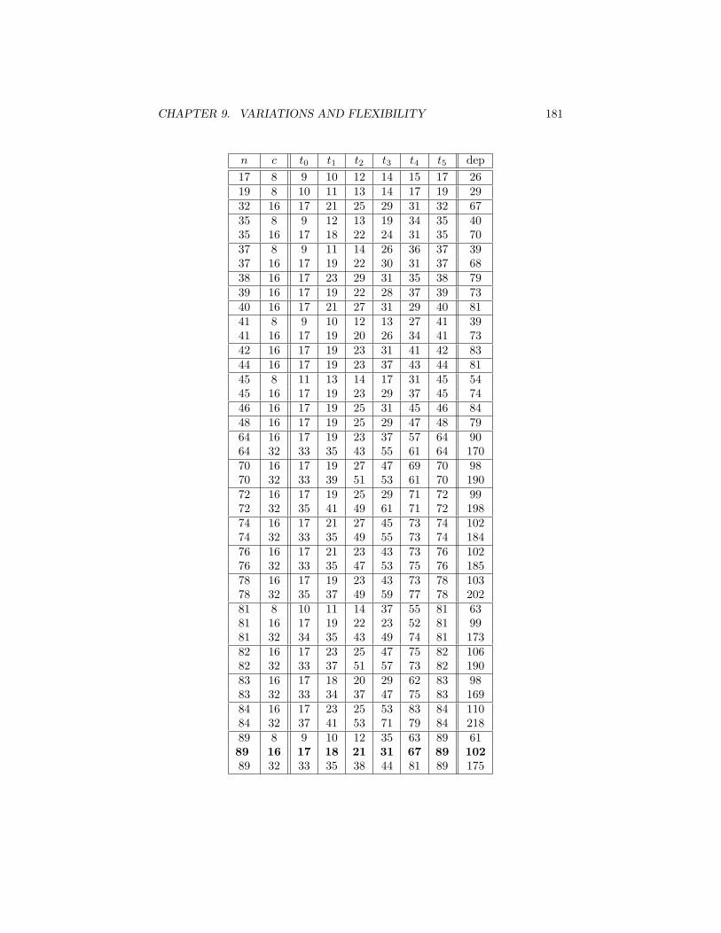
CHAPTER 9. VARIATIONS AND FLEXIBILITY 181
n c t0 t1 t2 t3 t4 t5 dep17 8 9 10 12 14 15 17 2619 8 10 11 13 14 17 19 2932 16 17 21 25 29 31 32 6735 8 9 12 13 19 34 35 4035 16 17 18 22 24 31 35 7037 8 9 11 14 26 36 37 3937 16 17 19 22 30 31 37 6838 16 17 23 29 31 35 38 7939 16 17 19 22 28 37 39 7340 16 17 21 27 31 29 40 8141 8 9 10 12 13 27 41 3941 16 17 19 20 26 34 41 7342 16 17 19 23 31 41 42 8344 16 17 19 23 37 43 44 8145 8 11 13 14 17 31 45 5445 16 17 19 23 29 37 45 7446 16 17 19 25 31 45 46 8448 16 17 19 25 29 47 48 7964 16 17 19 23 37 57 64 9064 32 33 35 43 55 61 64 17070 16 17 19 27 47 69 70 9870 32 33 39 51 53 61 70 19072 16 17 19 25 29 71 72 9972 32 35 41 49 61 71 72 19874 16 17 21 27 45 73 74 10274 32 33 35 49 55 73 74 18476 16 17 21 23 43 73 76 10276 32 33 35 47 53 75 76 18578 16 17 19 23 43 73 78 10378 32 35 37 49 59 77 78 20281 8 10 11 14 37 55 81 6381 16 17 19 22 23 52 81 9981 32 34 35 43 49 74 81 17382 16 17 23 25 47 75 82 10682 32 33 37 51 57 73 82 19083 16 17 18 20 29 62 83 9883 32 33 34 37 47 75 83 16984 16 17 23 25 53 83 84 11084 32 37 41 53 71 79 84 21889 8 9 10 12 35 63 89 6189 16 17 18 21 31 67 89 10289 32 33 35 38 44 81 89 175
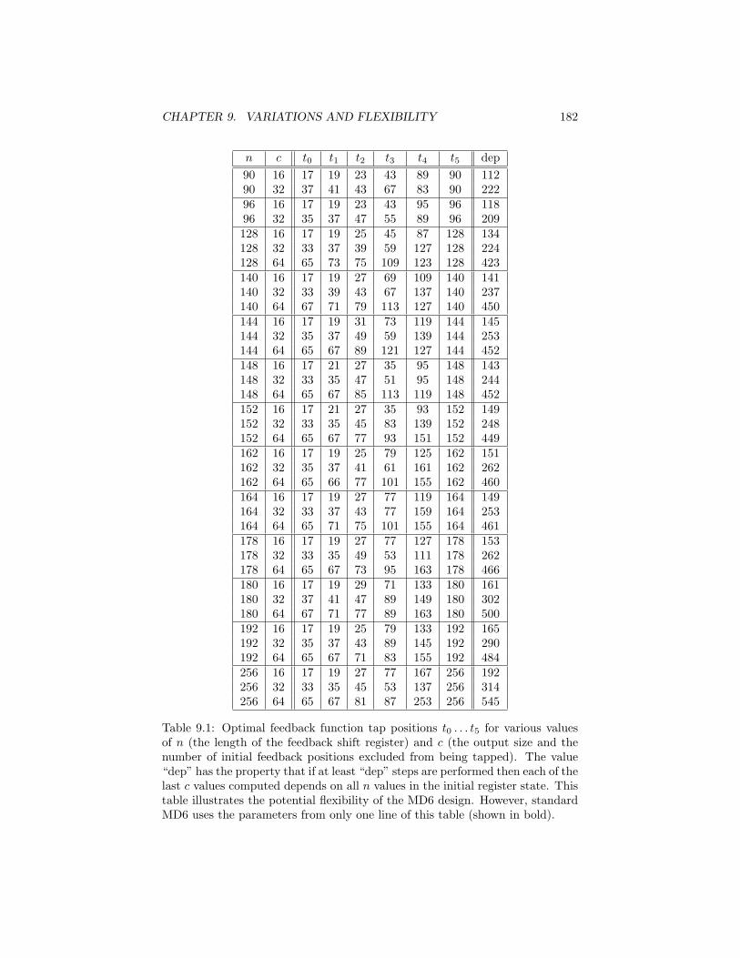
CHAPTER 9. VARIATIONS AND FLEXIBILITY 182
n c t0 t1 t2 t3 t4 t5 dep90 16 17 19 23 43 89 90 11290 32 37 41 43 67 83 90 22296 16 17 19 23 43 95 96 11896 32 35 37 47 55 89 96 209128 16 17 19 25 45 87 128 134128 32 33 37 39 59 127 128 224128 64 65 73 75 109 123 128 423140 16 17 19 27 69 109 140 141140 32 33 39 43 67 137 140 237140 64 67 71 79 113 127 140 450144 16 17 19 31 73 119 144 145144 32 35 37 49 59 139 144 253144 64 65 67 89 121 127 144 452148 16 17 21 27 35 95 148 143148 32 33 35 47 51 95 148 244148 64 65 67 85 113 119 148 452152 16 17 21 27 35 93 152 149152 32 33 35 45 83 139 152 248152 64 65 67 77 93 151 152 449162 16 17 19 25 79 125 162 151162 32 35 37 41 61 161 162 262162 64 65 66 77 101 155 162 460164 16 17 19 27 77 119 164 149164 32 33 37 43 77 159 164 253164 64 65 71 75 101 155 164 461178 16 17 19 27 77 127 178 153178 32 33 35 49 53 111 178 262178 64 65 67 73 95 163 178 466180 16 17 19 29 71 133 180 161180 32 37 41 47 89 149 180 302180 64 67 71 77 89 163 180 500192 16 17 19 25 79 133 192 165192 32 35 37 43 89 145 192 290192 64 65 67 71 83 155 192 484256 16 17 19 27 77 167 256 192256 32 33 35 45 53 137 256 314256 64 65 67 81 87 253 256 545
Table 9.1: Optimal feedback function tap positions t0 . . . t5 for various valuesof n (the length of the feedback shift register) and c (the output size and thenumber of initial feedback positions excluded from being tapped). The value“dep” has the property that if at least “dep” steps are performed then each of thelast c values computed depends on all n values in the initial register state. Thistable illustrates the potential flexibility of the MD6 design. However, standardMD6 uses the parameters from only one line of this table (shown in bold).
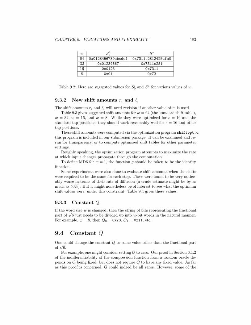
CHAPTER 9. VARIATIONS AND FLEXIBILITY 183
w S′0 S∗
64 0x0123456789abcdef 0x7311c2812425cfa032 0x01234567 0x7311c28116 0x0123 0x73118 0x01 0x73
Table 9.2: Here are suggested values for S′0 and S∗ for various values of w.
9.3.2 New shift amounts ri and `i
The shift amounts ri and `i will need revision if another value of w is used.Table 9.3 gives suggested shift amounts for w = 64 (the standard shift table),
w = 32, w = 16, and w = 8. While they were optimized for c = 16 and thestandard tap positions, they should work reasonably well for c = 16 and othertap positions.
These shift amounts were computed via the optimization program shiftopt.c;this program is included in our submission package. It can be examined and re-run for transparency, or to compute optimized shift tables for other parametersettings.
Roughly speaking, the optimization program attempts to maximize the rateat which input changes propagate through the computation.
To define MD6 for w = 1, the function g should be taken to be the identityfunction.
Some experiments were also done to evaluate shift amounts when the shiftswere required to be the same for each step. These were found to be very notice-ably worse in terms of their rate of diffusion (a crude estimate might be by asmuch as 50%). But it might nonetheless be of interest to see what the optimumshift values were, under this constraint. Table 9.4 gives these values.
9.3.3 Constant Q
If the word size w is changed, then the string of bits representing the fractionalpart of
√6 just needs to be divided up into w-bit words in the natural manner.
For example, w = 8, then Q0 = 0x73, Q1 = 0x11, etc.
9.4 Constant Q
One could change the constant Q to some value other than the fractional partof√
6.For example, one might consider setting Q to zero. Our proof in Section 6.1.2
of the indifferentiability of the compression function from a random oracle de-pends on Q being fixed, but does not require Q to have any fixed value. As faras this proof is concerned, Q could indeed be all zeros. However, some of the
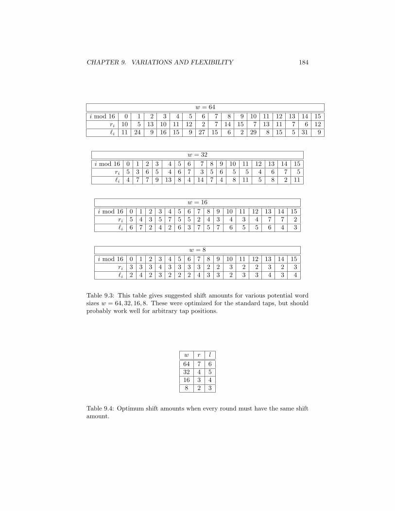
CHAPTER 9. VARIATIONS AND FLEXIBILITY 184
w = 64i mod 16 0 1 2 3 4 5 6 7 8 9 10 11 12 13 14 15
ri 10 5 13 10 11 12 2 7 14 15 7 13 11 7 6 12`i 11 24 9 16 15 9 27 15 6 2 29 8 15 5 31 9
w = 32i mod 16 0 1 2 3 4 5 6 7 8 9 10 11 12 13 14 15
ri 5 3 6 5 4 6 7 3 5 6 5 5 4 6 7 5`i 4 7 7 9 13 8 4 14 7 4 8 11 5 8 2 11
w = 16i mod 16 0 1 2 3 4 5 6 7 8 9 10 11 12 13 14 15
ri 5 4 3 5 7 5 5 2 4 3 4 3 4 7 7 2`i 6 7 2 4 2 6 3 7 5 7 6 5 5 6 4 3
w = 8i mod 16 0 1 2 3 4 5 6 7 8 9 10 11 12 13 14 15
ri 3 3 3 4 3 3 3 3 2 2 3 2 2 3 2 3`i 2 4 2 3 2 2 2 4 3 3 2 3 3 4 3 4
Table 9.3: This table gives suggested shift amounts for various potential wordsizes w = 64, 32, 16, 8. These were optimized for the standard taps, but shouldprobably work well for arbitrary tap positions.
w r l
64 7 632 4 516 3 48 2 3
Table 9.4: Optimum shift amounts when every round must have the same shiftamount.
CHAPTER 9. VARIATIONS AND FLEXIBILITY 185
algebraic attacks studied in Section 6.11.2 strongly suggest that MD6 may bestronger when Q is non-zero. Thus, setting Q = 0 is inadvisable.
However, setting Q to other “random-looking” constants should work as wellas the current choice; but it is important that Q remain a fixed constant.
9.5 Varying the number r of rounds
It is easy to vary the number r of rounds in the MD6 compression function.Indeed, we have made r an explicit (but optional) input parameter to MD6.
One may wish to do so to study the security of reduced-round versions (asin Chapter 6), to obtain different efficiency/security tradeoff points, or to studythe security of “crippled” versions of MD6.
Since MD6 is designed in a very conservative manner, it may happen thatover time we will gain confidence in the security of reduced-round versions ofMD6, and feel comfortable in using such reduced-round versions in practice, oreven adopting them in some standards. (At the moment, for example, we don’tknow how to break even 24-round MD6, much less 96 or 168 round versions.)However, MD6 is still a “new design,” and prudence would dictate erring on theside of conservatism, particularly given the history of hash function security todate.
9.6 Summary
The MD6 framework has tremendous flexibility. It is easy to create variantMD6 designs for study or for actual use in situations requiring non-standardparameterization. Of course, the security of such variants should be studiedcarefully before actual use.
Chapter 10
Acknowledgments
We’d like to thank Juniper Networks for an unrestricted gift of $15K to MITthat was used to support the development and analysis of MD6. (Just for therecord, Juniper Networks has no intellectual property rights to MD6.)
Thanks to the CILK team, both at MIT and at CILK Arts, for the helpwith porting MD6 to multicore processors and running benchmark tests onthese multicore processors. Thanks particularly to Charles Leiserson, BradleyKuszmaul, and Steve Lewin-Berlin.
Thanks to CSAIL’s TIG (The Infrastructure Group) for help with computinginfrastructure.
Thanks to Sarah Cheng, who assisted in some early discussion of parallelimplementations of MD6, and in some proof-reading of this report.
Thanks to Jean-Philippe Aumasson for providing his results on certain al-gebraic attacks, and allowing us to mention them in this report.
Thanks similarly to Itai Dinur for his collaborative efforts to evaluate theeffectiveness of his “cube attack” (developed with Adi Shamir) on MD6.
186
Chapter 11
Conclusions
This report has presented the MD6 cryptographic hash algorithm, for consider-ation by NIST as a SHA-3 candidate.
We have presented a detailed description of MD6, including its design ratio-nale, and have given in some detail our preliminary findings of its security andefficiency.
The standard MD6 design is very well-suited to take advantage of the forth-coming flood of multicore processors. The sequential variant of MD6 fits wellon an 8-bit processor. MD6 works very well on special-purpose processors (e.g.GPGPU’s), and is easy to implement effectively on special-purpose hardware.
From a security perspective, MD6 is very conservatively designed. While thestate of the art does not enable one to rigorously prove the security of a hashfunction against all attacks (indeed, we don’t know if P = NP ), we believe thatour security analyses of MD6, although they are only preliminary, provide strongjustification for believing that MD6 easily meets the security requirements fora SHA-3 standard.
The provable resistance of MD6 to differential and linear attacks is partic-ular noteworthy, as are the proofs that the compression function and mode ofoperation are indifferentiable from a random oracle.
We suggest that MD6 meets NIST’s stated goals of simplicity, efficiency ona variety of platforms, security, and flexibility, and would hope that MD6 willbe very seriously considered as a SHA-3 candidate hash algorithm.
187
Bibliography
[1] Onur Aciicmez, Cetin Kaya Koc, and Jean-Pierre Seifert. Predicting secretkeys via branch prediction. In CT-RSA, pages 225–242, 2007.
[2] Onur Aciicmez and Werner Schindler. A vulnerability in rsa implementa-tions due to instruction cache analysis and its demonstration on openssl.In CT-RSA, pages 256–273, 2008.
[3] Jee Hea An and Mihir Bellare. Constructing VIL-MACs from FIL-MACs: Message authentication under weakened assumptions. In Michael J.Wiener, editor, CRYPTO, volume 1666 of Lecture Notes in ComputerScience, pages 252–269. Springer, 1999.
[4] Atmel. Avr 8-bit RISC. http://www.atmel.com/dyn/products/tools.asp?family_id=607.
[5] AVR microcontroller. http://en.wikipedia.org/wiki/Atmel_AVR.
[6] Mihir Bellare, Ran Canetti, and Hugo Krawczyk. Keying hash functionsfor message authentication. In N. Koblitz, editor, Proc. CRYPTO ’96,number 1109 in LNCS, pages 1–15. Springer, 1996. Full version at http://www-cse.ucsd.edu/~mihir/papers/hmac.html.
[7] Mihir Bellare, Roch Guerin, and Phillip Rogaway. XOR MAC’s: Newmethods for message authentication using finite pseudorandom functions.In D. Coppersmith, editor, Proc. CRYPTO ’95, number 963 in LNCS,pages 15–28. Springer, 1995.
[8] Mihir Bellare, Joe Kilian, and Phillip Rogaway. The Security of the Ci-pher Block Chaining Message Authentication Code. J. Comput. Syst. Sci.,61(3):362–399, 2000.
[9] Mihir Bellare, Krzysztof Pietrzak, and Phillip Rogaway. Improved SecurityAnalyses for CBC MACs. In Victor Shoup, editor, CRYPTO, volume 3621of Lecture Notes in Computer Science, pages 527–545. Springer, 2005.
[10] Mihir Bellare and Thomas Ristenpart. Hash functions in the dedicated-keysetting: Design choices and mpp transforms. Cryptology ePrint Archive,Report 2007/271, 2007. http://eprint.iacr.org/2007/271.pdf.
188
BIBLIOGRAPHY 189
[11] Mihir Bellare and Phillip Rogaway. Random Oracles are Practical: AParadigm for Designing Efficient Protocols. In ACM Conference onComputer and Communications Security, pages 62–73, 1993.
[12] Daniel J. Bernstein. Cache-timing attacks on AES, 2005. http://cr.yp.to/papers.html#cachetiming.
[13] Guido Bertoni, Joan Daeman, Michael Peeters, and Gilles Van Ass-che. Sponge functions, May 2007. http://www.csrc.nist.gov/pki/HashWorkshop/PublicComments/2007May.html.
[14] Guido Bertoni, Joan Daemen, Michael Peeters, and Gilles Van Assche. Onthe indifferentiability of the sponge construction. In Proc. Eurocrypt 2008,volume 4965 of LNCS, pages 181–197. Springer, 2008.
[15] E. Biham and A. Shamir. Differential cryptanalysis of DES-like cryptosys-tems. J. Cryptology, 4(1):3–72, 1991.
[16] Eli Biham and Rafi Chen. Near-collisions of SHA-0 . In Advancesin Cryptology – CRYPTO ’04, number 3152 in LNCS, pages 290–305.Springer, 2004.
[17] Eli Biham, Rafi Chen, Antoine Joux, Patrick Carribault, ChristopheLemuet, and William Jalby. Collisions of SHA-0 and reduced SHA-1. InAdvances in Cryptology – EUROCRYPT ’05, number 3621 in LNCS, pages36–57, 2005.
[18] Eli Biham and Orr Dunkelman. A framework for iterative hash func-tions – HAIFA, August 2006. NIST 2nd Hash Function Workshop,Santa Barbara. http://www.cs.technion.ac.il/users/wwwb/cgi-bin/tr-info.cgi?2007/CS/CS-2007-15.
[19] J. Black, P. Rogaway, and T. Shrimpton. Black-box analysis of theblockcipher-based hash-function constructions from PGV. In Proc. Crypto’02, volume 2442 of LNCS, pages 103–118. Springer, 2002. http://www.cs.colorado.edu/~jrblack/papers/hash.pdf.
[20] John Black, Martin Cochran, and Thomas Shrimpton. On the impossibilityof highly-efficient blockcipher-based hash functions. In R. Cramer, editor,Proc. Eurocrypt 2005, volume 3494 of LNCS, pages 526–541. Springer,2005. http://www.cs.colorado.edu/~jrblack/papers/ohash.pdf.
[21] Sergey Bratus and Igor Pak. Fast constructive recognition of a black boxgroup isomorphic to sn or an using goldbach’s conjecture. J. SymbolicComputation, 29:33–57, 2000.
[22] David Brumley and Dan Boneh. Remote timing attacks are practical.Computer Networks, 48(5):701–716, 2005.

BIBLIOGRAPHY 190
[23] Ran Canetti. Towards realizing random oracles: Hash functions that hideall partial information. In Lecture Notes in Computer Science, volume1294, pages 455–469, 1997.
[24] Ran Canetti, Oded Goldreich, and Shai Halevi. The Random OracleMethodology, Revisited. CoRR, cs.CR/0010019, 2000. informal publica-tion.
[25] Christophe De Canniere and Christian Rechberger. Finding SHA-1 char-acteristics: General results and applications. In Proc. ASIACRYPT ’06,volume 4284 of LNCS, pages 1–20. Springer, 2006.
[26] CardLogix. Smart card product selection guide, 2005. http://www.cardlogix.com/pdf/ProductSelectionGuide.pdf.
[27] Florent Chabaud and Antoine Joux. Differential collisions of SHA-0 .In Advances in Cryptology – CRYPTO ’98, number 1462 in LNCS, pages56–71. Springer, 1998.
[28] Ricardo Chaves, Georgi Kuzmanov, Leonel Sousa, and Stamatis Vassil-iadis. Improving sha-2 hardware implementations. In In Workshop onCryptographic Hardware and Embedded Systems, CHES 2006, 2006.
[29] Debra L. Cook, John Ioannidis, Angelos D. Keromytis, and Jake Luck.Cryptographics: Secret key cryptography using graphics cards. In CT-RSA,pages 334–350, 2005.
[30] D. Coppersmith and E. Grossman. Generators for certain alternatinggroups with applications to cryptology. SIAM J. Applied Mathematics,29:624–627, 1975.
[31] Jean-Sebastien Coron, Yevgeniy Dodis, Cecile Malinaud, and PrashantPuniya. Merkle-Damgard revisited: How to construct a hash function.In Advances in Cryptology – CRYPTO ’05, number 3621 in LNCS, pages430–448. Springer, 2005.
[32] Christopher Yale Crutchfield. Security proofs for the MD6 hashfunction mode of operation. Master’s thesis, MIT EECS De-partment, 2008. http://groups.csail.mit.edu/cis/theses/crutchfield-masters-thesis.pdf.
[33] Joan Daemen and Vincent Rijmen. The Design of Rijndael: AES–theAdvanced Encryption Standard. Springer, 2002.
[34] Ivan Bjerre Damgard. A design principle for hash functions. In G. Brassard,editor, Advances in Cryptology – CRYPTO ’89, number 435 in LNCS,pages 416–427. Springer, 1990.
BIBLIOGRAPHY 191
[35] Yevgeniy Dodis, Krzysztof Pietrzak, and Prashant Puniya. A new modeof operation for block ciphers and length-preserving MACs. In Nigel P.Smart, editor, EUROCRYPT, volume 4965 of Lecture Notes in ComputerScience, pages 198–219. Springer, 2008.
[36] Hakan Englund, Thomas Johansson, and Meltem Sonmez Turan. Aframework for chosen iv statistical analysis of stream ciphers. InProc. Indocrypt ’07, volume 4859, pages 268–281. Springer, Dec. 2007.http://www.impan.gov.pl/BC/Program/conferences/07Crypt-abs/Turan%20-%20A%20framework%20for%20Chosen%20IV%20Statistical%20Analysis.pdf.
[37] Amos Fiat and Adi Shamir. How to Prove Yourself: Practical Solutionsto Identification and Signature Problems. In Andrew M. Odlyzko, editor,CRYPTO, volume 263 of Lecture Notes in Computer Science, pages 186–194. Springer, 1986.
[38] Claudia Fiorini, Enrico Martinelli, and Fabio Massacci. How to fake anrsa signature by encoding modular root finding as a sat problem. DiscreteApplied Mathematics, 130(2):101–127, 2003.
[39] Simon Fischer, Shahram Khazaei, and Willi Meier. Chosen IV statisticalanalysis for key recovery attacks on stream ciphers. In Serge Vaudenay,editor, AFRICACRYPT, volume 5023 of LNCS, pages 236–245. Springer,2008.
[40] International Technology Roadmap for Semiconductors. International tech-nology roadmap for semiconductors 2007, 2007. http://www.itrs.net/Links/2007ITRS/Home2007.htm.
[41] Oded Goldreich, Shafi Goldwasser, and Silvio Micali. On the CryptographicApplications of Random Functions. In CRYPTO, pages 276–288, 1984.
[42] Oded Goldreich, Shafi Goldwasser, and Silvio Micali. How to ConstructRandom Functions. J. ACM, 33(4):792–807, 1986.
[43] Owen Harrison and John Waldron. Practical symmetric key cryptogra-phy on modern graphics hardware. In Proc. USENIX ’08, pages 195–209.USENIX Assoc., 2008. http://www.usenix.org/events/sec08/tech/harrison.html.
[44] Jonathan J. Hoch and Adi Shamir. Breaking the ICE—finding multicol-lisions in iterated concatenated and expanded (ICE) hash functions. InProc. Fast Software Encryption 2006, volume 4047 of LNCS, pages 179–194. Springer, 2006.
[45] Kimmo Jarvinen, Matti Tommiska, and Jorma Skytta. Hardware imple-mentation analysis of the md5 hash algorithm. In HICSS ’05: Proceedingsof the Proceedings of the 38th Annual Hawaii International Conference on
BIBLIOGRAPHY 192
System Sciences (HICSS’05) - Track 9, page 298.1, Washington, DC, USA,2005. IEEE Computer Society.
[46] Antoine Joux. Multicollisions in iterated hash functions. In Advancesin Cryptology – CRYPTO ’04, number 3152 in LNCS, pages 306–316.Springer, 2004.
[47] Dejan Jovanovic and Predrag Janicic. Logical analysis of hash functions.In FroCos, pages 200–215, 2005.
[48] Charanjit S. Jutla and Anindya C. Patthak. A simple and provably goodcode for SHA message expansion, 2005. http://eprint.iacr.org/2005/247.
[49] Burt Kaliski and Matt Robshaw. Message authentication with MD5.RSA Labs Cryptobytes, 1(1):5–8, 1995. http://citeseer.ist.psu.edu/433722.html.
[50] John Kelsey and Bruce Schneier. Second preimages on n-bit hash functionsfor much less than 2n. In Advances in Cryptology – EUROCRYPT ’05,number 3494 in LNCS, pages 474–490, 2005.
[51] P. Kitsos and O. Koufopavlou. Efficient architecture and hardware im-plementation of the whirlpool hash function. IEEE Trans. ConsumerElectronics, 50(1):218–213, Feb 2004.
[52] Poonacha Kongetira, Kathirgamar Aingaran, and Kunle Olukotun. Nia-gara: A 32-way multithreaded sparc processor. IEEE Micro, 25(2):21–29,2005.
[53] Pierre L’Ecuyer and Richard Simard. Testu01: A c library for empiricaltesting of random number generators. ACM Trans. Math. Softw., 33(4):22,2007.
[54] Stefan Lucks. Design principles for iterated hash functions, Sep. 29 2004.http://eprint.iacr.org/2004/253.
[55] Stefan Lucks. A failure-friendly design principle for hash functions.In Proceedings of Asiacrypt 2005, number 3788 in Lecture Notes inComputer Science, pages 474–494. Springer-Verlag, 2005. http://www.springerlink.com/content/f868557868208018/.
[56] G. Marsaglia. Xorshift RNGs. J. Stat. Soft., 8(14):1–6, 2003. http://www.jstatsoft.org/v08/i14/xorshift.pdf.
[57] Fabio Massacci. Using walk-sat and rel-sat for cryptographic key search.In IJCAI, pages 290–295, 1999.
[58] M. Matsui. Linear cryptanalysis method for DES cipher. In Proc.EUROCRYPT’93, volume 765 of LNCS, pages 386–397. Springer, 1993.
BIBLIOGRAPHY 193
[59] U. Maurer, R. Renner, and C. Holenstein. Indifferentiability, impossibilityresults on reductions, and applications to the random oracle methodology.In Proc. TCC ’04, volume 2951 of LNCS, pages 21–39. Springer, Feb. 2004.
[60] Ueli M. Maurer. Indistinguishability of Random Systems. In Lars R. Knud-sen, editor, EUROCRYPT, volume 2332 of Lecture Notes in ComputerScience, pages 110–132. Springer, 2002.
[61] Ueli M. Maurer and Krzysztof Pietrzak. Composition of Random Systems:When Two Weak Make One Strong. In Moni Naor, editor, TCC, volume2951 of Lecture Notes in Computer Science, pages 410–427. Springer, 2004.
[62] Maire McLoone and Ciaran McIvor. High-speed & low area hardware ar-chitectures of the whirlpool hash function. J. VLSI Signal Process. Syst.,47(1):47–57, 2007.
[63] Alfred J. Menezes, Paul C. van Oorschot, and Scott A. Vanstone. Handbookof Applied Cryptography. CRC Press, 1997. http://www.cacr.math.uwaterloo.ca/hac/.
[64] Ralph C. Merkle. One way hash functions and DES . In Advances inCryptology – CRYPTO ’89, number 435 in LNCS, pages 428–446. Springer,1990.
[65] Ralphc C. Merkle. Secrecy, Authentication, and Public Key Systems. PhDthesis, Stanford University, 1982. UMI Research Press.
[66] H. E. Michail, A. P. Kakarountas, G. Theodoridis, and C. E. Goutis. Alow-power and high-throughput implementation of the sha-1 hash function.In ICCOMP’05: Proceedings of the 9th WSEAS International Conferenceon Computers, pages 1–6, Stevens Point, Wisconsin, USA, 2005. WorldScientific and Engineering Academy and Society (WSEAS).
[67] Ilya Mironov and Lintao Zhang. Applications of sat solvers to cryptanalysisof hash functions. In SAT, pages 102–115, 2006.
[68] M. Nandi and D. R. Stinson. Multicollision attacks on a class of hashfunctions. Cryptology ePrint Archive, Report 2004/330, 2004. http://eprint.iacr.org/2004/330.
[69] M. Nandi and D. R. Stinson. Multicollision attacks on some generalizedsequential hash functions. IEEE Trans. Inform. Theory, 53(2):759–767,Feb. 2007.
[70] National Institute of Standards and Technology. Announcing request forcandidate algorithm nominations for a new cryptographic hash algorithm(sha-3) family. Federal Register Notices, 72(212):62212–62220, Nov. 22007. http://csrc.nist.gov/groups/ST/hash/documents/FR_Notice_Nov07.pdf.
BIBLIOGRAPHY 194
[71] National Institute of Standards and Technology. Recommenda-tion for key management — part 1: General (revised), March2007. http://csrc.nist.gov/groups/ST/toolkit/documents/SP800-57Part1_3-8-07.pdf.
[72] National Institute of Standards and Technology. The keyed-hash messageauthentication code (HMAC). NIST Federal Information Processing Stan-dards Publication FIPS 198-1, July 2008.
[73] Sean O’Neil. Algebraic structure defectoscopy. Cryptology ePrint Archive,Report 2007/378, 2007.
[74] Dag Arne Osvik, Adi Shamir, and Eran Tromer. Cache attacks and coun-termeasures: the case of AES. In Proc. RSA Conference CryptographersTrack (CT-RSA), number 3860 in LNCS, pages 1–20. Springer, 2006.
[75] Francois Panneton and Pierre L’Ecuyer. On the Xorshift random numbergenerators. ACM Trans. Modeling and Computer Simulation, 15(4):346–361, Oct. 2005.
[76] Colin Percival. Cache missing for fun and profit, 2005. http://www.daemonology.net/papers/htt.pdf.
[77] Krzysztof Pietrzak. Indistinguishability and Composition of RandomSystems. PhD thesis, ETH Zurich, 2006. Reprint as vol. 6 of ETH Seriesin Information Security and Cryptography, ISBN 3-86626-063-7, Hartung-Gorre Verlag, Konstanz, 2006.
[78] Norbert Pramstaller, Christian Rechberger, and Vincent Rijmen. A com-pact fpga implementation of the hash function whirlpool. In FPGA ’06:Proceedings of the 2006 ACM/SIGDA 14th international symposium onField programmable gate arrays, pages 159–166, New York, NY, USA,2006. ACM.
[79] B. Preneel, R. Govaerts, and J. Vandewalle. Hash functions based on blockciphers: A synthetic approach. In Proc. Crypto ’93, volume 773 of LNCS,pages 368–378. Springer, 1993.
[80] Bart Preneel. Hash functions – present state of art, 2005. ECrypt Confer-ence on Hash Functions.
[81] Bart Preneel, Rene Govaerts, and Joos Vanderwalle. Differential crypt-analysis of hash functions based on block ciphers. In Proc. Computer andCommunications Security, pages 183–188. ACM, 1993.
[82] Bart Preneel and Paul C. van Oorschot. MDx-MAC and building fastMACs from hash functions. In D. Coppersmith, editor, Proc. CRYPTO’96, number 963 in LNCS, pages 1–14. Springer, 1995.
BIBLIOGRAPHY 195
[83] Bart Preneel and Paul C. van Oorschot. On the security of two MACalgorithms. In U. Maurer, editor, Proc. Eurocrypt ’96, number 1070 inLNCS, pages 19–32. Springer, 1996.
[84] AJ Rivest. Mice learn! PhD thesis, 2011.
[85] Ronald L. Rivest. Abelian square-free dithering for iteratedhash functions, 2005. http://people.csail.mit.edu/rivest/Rivest-AbelianSquareFreeDitheringForIteratedHashFunctions.pdf.
[86] Phillip Rogaway. Formalizing human ignorance: Collision-resistant hashingwithout the keys. In Proc. Vietcrypt ’06, volume 4341 of LNCS, pages 221–228. Springer, 2006.
[87] Phillip Rogaway and Thmas Shrimpton. Cryptographic hash-function ba-sics: Definitions, implications, and separations for preimage resistance,second-preimage resistance, and collision-resistance. In Proc. Fast SoftwareEncryption 2004, number 3017 in LNCS, pages 371–388. Springer, 2004.
[88] P. Sarkar and P. J. Schellenberg. A parallelizable design principle for cryp-tographic hash functions, 2002. http://eprint.iacr.org/2002/031.
[89] Claus P. Schnorr and Serge Vaudenay. Black box cryptanalysis of hashnetworks based on multipermutations. In Proceedings EUROCRYPT ’94,volume 950 of Lecture Notes in Computer Science, pages 47–57. Springer,1995.
[90] N. Sklavos and O. Koufopavlou. Implementation of the sha-2 hash familystandard using fpgas. J. Supercomput., 31(3):227–248, 2005.
[91] Andrew V. Sutherland. Order Computation in Generic Groups. PhD thesis,MIT Department of Mathematics, 2007. http://groups.csail.mit.edu/cis/theses/sutherland-phd.pdf.
[92] Eran Tromer. Hardware-Based Cryptanalysis. PhD thesis, Weizmann In-stitute of Science, May 2007.
[93] Yukiyasu Tsunoo, Teruo Saito, Tomoyasu Suzaki, Maki Shigeri, and HiroshiMiyauchi. Cryptanalysis of DES implemented on computers with cache. InCHES, pages 62–76, 2003.
[94] Xiaoyun Wang, Xuejia Lai, Dengguo Feng, Hui Chen, and Xiuyuan Yu.Cryptanalysis of the hash functions MD4 and RIPEMD. In Proc. Eurocrypt2005, number 3494 in LNCS, pages 1– 18. Springer, 2005.
[95] Xiaoyun Wang, Yiqun Lisa Yin, and Hongbo Yu. Finding collisions in thefull SHA-1. In Proc. CRYPTO 2005, number 3621 in LNCS, pages 17–36.Springer, 2005.
BIBLIOGRAPHY 196
[96] Xiaoyun Wang and Hongbo Yu. How to break MD5 and other hash func-tions. In Proc. EUROCRYPT 2005, number 3494 in LNCS, pages 19–35.Springer, 2005.
[97] Xiaoyun Wang, Hongbo Yu, and Yiqun Lisa Yin. Efficient collision searchattacks on SHA-0. In Proc. CRYPTO 2005, number 3621 in LNCS, pages1–16. Springer, 2005.
[98] Hongbo Yu and Xiaoyun Wang. Multicollision attack on the compressionfunctions of MD4 and 3-pass HAVAL. IACR eprint, 2007. http://eprint.iacr.org/2007/085/.
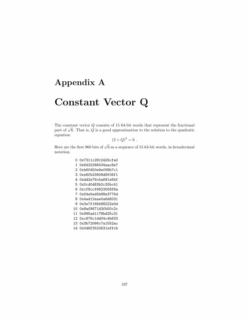
Appendix A
Constant Vector Q
The constant vector Q consists of 15 64-bit words that represent the fractionalpart of
√6. That is, Q is a good approximation to the solution to the quadratic
equation:(2 +Q)2 = 6 .
Here are the first 960 bits of√
6 as a sequence of 15 64-bit words, in hexadecimalnotation.
0 0x7311c2812425cfa01 0x6432286434aac8e72 0xb60450e9ef68b7c13 0xe8fb23908d9f06f14 0xdd2e76cba691e5bf5 0x0cd0d63b2c30bc416 0x1f8ccf6823058f8a7 0x54e5ed5b88e3775d8 0x4ad12aae0a6d60319 0x3e7f16bb88222e0d
10 0x8af8671d3fb50c2c11 0x995ad1178bd25c3112 0xc878c1dd04c4b63313 0x3b72066c7a1552ac14 0x0d6f3522631effcb
197
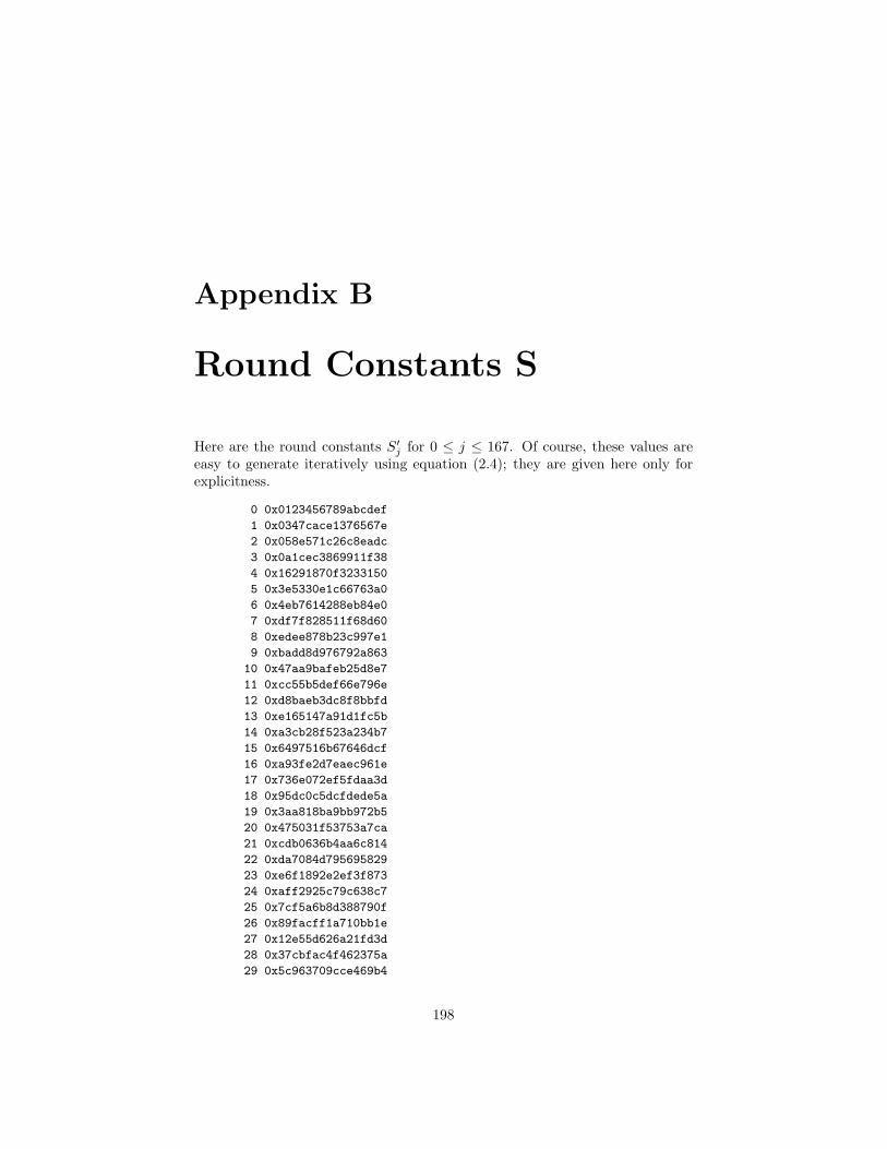
Appendix B
Round Constants S
Here are the round constants S′j for 0 ≤ j ≤ 167. Of course, these values areeasy to generate iteratively using equation (2.4); they are given here only forexplicitness.
0 0x0123456789abcdef
1 0x0347cace1376567e
2 0x058e571c26c8eadc
3 0x0a1cec3869911f38
4 0x16291870f3233150
5 0x3e5330e1c66763a0
6 0x4eb7614288eb84e0
7 0xdf7f828511f68d60
8 0xedee878b23c997e1
9 0xbadd8d976792a863
10 0x47aa9bafeb25d8e7
11 0xcc55b5def66e796e
12 0xd8baeb3dc8f8bbfd
13 0xe165147a91d1fc5b
14 0xa3cb28f523a234b7
15 0x6497516b67646dcf
16 0xa93fe2d7eaec961e
17 0x736e072ef5fdaa3d
18 0x95dc0c5dcfdede5a
19 0x3aa818ba9bb972b5
20 0x475031f53753a7ca
21 0xcdb0636b4aa6c814
22 0xda7084d795695829
23 0xe6f1892e2ef3f873
24 0xaff2925c79c638c7
25 0x7cf5a6b8d388790f
26 0x89facff1a710bb1e
27 0x12e55d626a21fd3d
28 0x37cbfac4f462375a
29 0x5c963709cce469b4
198

APPENDIX B. ROUND CONSTANTS S 199
30 0xe93c6c129dec9ac8
31 0xb36898253ffdbf11
32 0x55d1b04b5bdef123
33 0xfab2e097b7b92366
34 0x877501ae4b5345ed
35 0x0dfb03dc96a7ce7b
36 0x1ae70539296a52d6
37 0x27cf0a7372f4e72c
38 0x6c9f16e7c5cd0978
39 0xb92f2f4e8f9f1bd0
40 0x435f5c9d1b3b3c21
41 0xc5aff9bb36577462
42 0xca5e33f748abace5
43 0xd6ac656f9176d56b
44 0xff588ade22c96ff7
45 0x8da1973c6593904f
46 0x1a42ac78ef26a09f
47 0x2685d8f1fa69c1be
48 0x6f0a7162d4f242dc
49 0xbd14a2c5adc4c738
50 0x4b39c70a7f8d4951
51 0xd5624c14db1fdba2
52 0xfbc4d829b63a7ce5
53 0x848970524854b56b
54 0x0913a0a490adeff7
55 0x1336c1c9217e104e
56 0x357d431362d8209c
57 0x5bebc427e5b041b8
58 0xe4d6484eef40c2d0
59 0xa9bcd09dfa814721
60 0x726961bad503c963
61 0x96d383f5ae065be6
62 0x3fb6856a7808fc6d
63 0x4c7d8ad4d01134fa
64 0xd8ea9729a0236d54
65 0xe1d5ac52606797a9
66 0xa2bad8a4e0eaa8f3
67 0x676571c9e1f5d947
68 0xadcba312e3ce7b8e
69 0x7a96c425e798bc9d
70 0x873d484aeb31f5ba
71 0x0d6bd095f6422ed5
72 0x1bd661aac884532a
73 0x24bc83d5910ce574
74 0x6969852a221d0fc8
75 0xb3d28a54643f1010
76 0x54b596a8ec5b2021
77 0xf97aafd1fcb74062
78 0x83e5dd22dd4bc0e5
79 0x04ca7a45be96416b
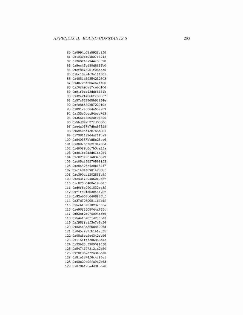
APPENDIX B. ROUND CONSTANTS S 200
80 0x0994b68a5928c3f6
81 0x1239ef94b271444c
82 0x36621da944c3cc98
83 0x5ec43bd38d8655b0
84 0xef8875261f08eec0
85 0xbc10aa4c3a111301
86 0x4831d69854232503
87 0xd0726fb0ac674f06
88 0xf0f49de17cebd10d
89 0x91f9bb43ddf6631b
90 0x32e2f486bfc88537
91 0x57c5298d5b918f4e
92 0xfc8b539bb722919c
93 0x8917e5b64a65a2b9
94 0x133e0bec94eec7d3
95 0x356c15592df94826
96 0x5bd82ab37fd3d86c
97 0xe4a057e7dba678f8
98 0xa940ed4eb768b951
99 0x73811a9d4af1fba3
100 0x940337bb95c23ce6
101 0x38076df62f84756d
102 0x400f9b6c7b0caffa
103 0xc01eb4d8d61dd054
104 0xc02de931a83e60a9
105 0xc05a1262705881f3
106 0xc0a426c4c0b18247
107 0xc1484f098142868f
108 0xc390dc1202858b9f
109 0xc4317824050e9cbf
110 0xc873b0480e19b5df
111 0xd0f6e0901832ee3f
112 0xf1fd01a03045125f
113 0x92eb03c0408f26bf
114 0x37d70500811b4bdf
115 0x5cbf0a010237dc3e
116 0xe96f1603044a745c
117 0xb3df2e070c94acb9
118 0x54af5e0f1d2dd5d3
119 0xf95ffe1f3e7e6e26
120 0x83ae3e3f58d8926d
121 0x045c7e7fb1b1a6fb
122 0x08a8befe4342cb56
123 0x1151ff7c86855dac
124 0x33b23cf9090ff6f8
125 0x54747973121a2b50
126 0xf8f8b2e724345da0
127 0x81e1e74f6c4cf6e1
128 0x02c20c9ffc9d2b63
129 0x078419bedd3f5de6
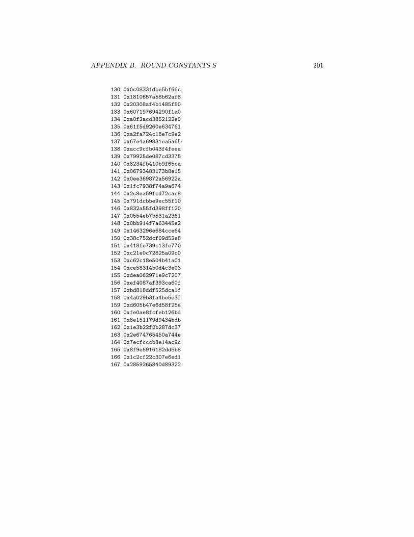
APPENDIX B. ROUND CONSTANTS S 201
130 0x0c0833fdbe5bf66c
131 0x1810657a58b62af8
132 0x20308af4b1485f50
133 0x607197694290f1a0
134 0xa0f2acd3852122e0
135 0x61f5d9260e634761
136 0xa2fa724c18e7c9e2
137 0x67e4a69831ea5a65
138 0xacc9cfb043f4feea
139 0x79925de087cd3375
140 0x8234fb410b9f65ca
141 0x06793483173b8e15
142 0x0ee369872a56922a
143 0x1fc7938f74a9a674
144 0x2c8ea59fcd72cac8
145 0x791dcbbe9ec55f10
146 0x832a55fd398ff120
147 0x0554eb7b531a2361
148 0x0bb914f7a63445e2
149 0x1463296e684cce64
150 0x38c752dcf09d52e8
151 0x418fe739c13fe770
152 0xc21e0c72825a09c0
153 0xc62c18e504b41a01
154 0xce58314b0d4c3e03
155 0xdea062971e9c7207
156 0xef4087af393ca60f
157 0xbd818ddf525dca1f
158 0x4a029b3fa4be5e3f
159 0xd605b47e6d58f25e
160 0xfe0ae8fcfeb126bd
161 0x8e151179d9434bdb
162 0x1e3b22f2b287dc37
163 0x2e674765450a744e
164 0x7ecfcccb8e14ac9c
165 0x8f9e5916182dd5b8
166 0x1c2cf22c307e6ed1
167 0x2859265840d89322
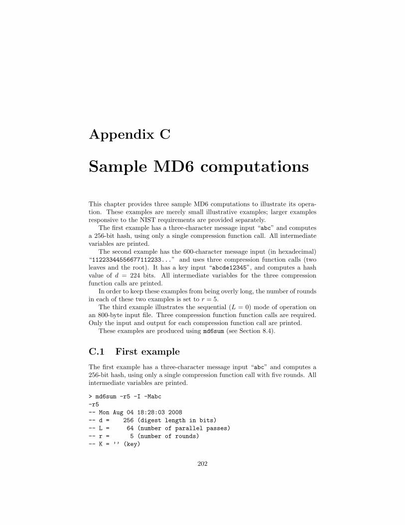
Appendix C
Sample MD6 computations
This chapter provides three sample MD6 computations to illustrate its opera-tion. These examples are merely small illustrative examples; larger examplesresponsive to the NIST requirements are provided separately.
The first example has a three-character message input “abc” and computesa 256-bit hash, using only a single compression function call. All intermediatevariables are printed.
The second example has the 600-character message input (in hexadecimal)“11223344556677112233...” and uses three compression function calls (twoleaves and the root). It has a key input “abcde12345”, and computes a hashvalue of d = 224 bits. All intermediate variables for the three compressionfunction calls are printed.
In order to keep these examples from being overly long, the number of roundsin each of these two examples is set to r = 5.
The third example illustrates the sequential (L = 0) mode of operation onan 800-byte input file. Three compression function function calls are required.Only the input and output for each compression function call are printed.
These examples are produced using md6sum (see Section 8.4).
C.1 First example
The first example has a three-character message input “abc” and computes a256-bit hash, using only a single compression function call with five rounds. Allintermediate variables are printed.
> md6sum -r5 -I -Mabc-r5-- Mon Aug 04 18:28:03 2008-- d = 256 (digest length in bits)-- L = 64 (number of parallel passes)-- r = 5 (number of rounds)-- K = ’’ (key)
202
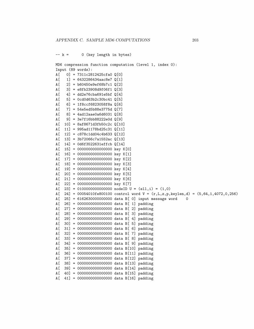
APPENDIX C. SAMPLE MD6 COMPUTATIONS 203
-- k = 0 (key length in bytes)
MD6 compression function computation (level 1, index 0):Input (89 words):A[ 0] = 7311c2812425cfa0 Q[0]A[ 1] = 6432286434aac8e7 Q[1]A[ 2] = b60450e9ef68b7c1 Q[2]A[ 3] = e8fb23908d9f06f1 Q[3]A[ 4] = dd2e76cba691e5bf Q[4]A[ 5] = 0cd0d63b2c30bc41 Q[5]A[ 6] = 1f8ccf6823058f8a Q[6]A[ 7] = 54e5ed5b88e3775d Q[7]A[ 8] = 4ad12aae0a6d6031 Q[8]A[ 9] = 3e7f16bb88222e0d Q[9]A[ 10] = 8af8671d3fb50c2c Q[10]A[ 11] = 995ad1178bd25c31 Q[11]A[ 12] = c878c1dd04c4b633 Q[12]A[ 13] = 3b72066c7a1552ac Q[13]A[ 14] = 0d6f3522631effcb Q[14]A[ 15] = 0000000000000000 key K[0]A[ 16] = 0000000000000000 key K[1]A[ 17] = 0000000000000000 key K[2]A[ 18] = 0000000000000000 key K[3]A[ 19] = 0000000000000000 key K[4]A[ 20] = 0000000000000000 key K[5]A[ 21] = 0000000000000000 key K[6]A[ 22] = 0000000000000000 key K[7]A[ 23] = 0100000000000000 nodeID U = (ell,i) = (1,0)A[ 24] = 00054010fe800100 control word V = (r,L,z,p,keylen,d) = (5,64,1,4072,0,256)A[ 25] = 6162630000000000 data B[ 0] input message word 0A[ 26] = 0000000000000000 data B[ 1] paddingA[ 27] = 0000000000000000 data B[ 2] paddingA[ 28] = 0000000000000000 data B[ 3] paddingA[ 29] = 0000000000000000 data B[ 4] paddingA[ 30] = 0000000000000000 data B[ 5] paddingA[ 31] = 0000000000000000 data B[ 6] paddingA[ 32] = 0000000000000000 data B[ 7] paddingA[ 33] = 0000000000000000 data B[ 8] paddingA[ 34] = 0000000000000000 data B[ 9] paddingA[ 35] = 0000000000000000 data B[10] paddingA[ 36] = 0000000000000000 data B[11] paddingA[ 37] = 0000000000000000 data B[12] paddingA[ 38] = 0000000000000000 data B[13] paddingA[ 39] = 0000000000000000 data B[14] paddingA[ 40] = 0000000000000000 data B[15] paddingA[ 41] = 0000000000000000 data B[16] padding
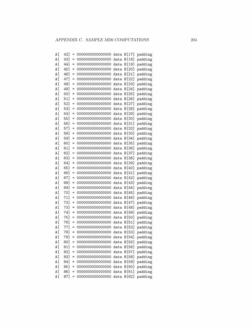
APPENDIX C. SAMPLE MD6 COMPUTATIONS 204
A[ 42] = 0000000000000000 data B[17] paddingA[ 43] = 0000000000000000 data B[18] paddingA[ 44] = 0000000000000000 data B[19] paddingA[ 45] = 0000000000000000 data B[20] paddingA[ 46] = 0000000000000000 data B[21] paddingA[ 47] = 0000000000000000 data B[22] paddingA[ 48] = 0000000000000000 data B[23] paddingA[ 49] = 0000000000000000 data B[24] paddingA[ 50] = 0000000000000000 data B[25] paddingA[ 51] = 0000000000000000 data B[26] paddingA[ 52] = 0000000000000000 data B[27] paddingA[ 53] = 0000000000000000 data B[28] paddingA[ 54] = 0000000000000000 data B[29] paddingA[ 55] = 0000000000000000 data B[30] paddingA[ 56] = 0000000000000000 data B[31] paddingA[ 57] = 0000000000000000 data B[32] paddingA[ 58] = 0000000000000000 data B[33] paddingA[ 59] = 0000000000000000 data B[34] paddingA[ 60] = 0000000000000000 data B[35] paddingA[ 61] = 0000000000000000 data B[36] paddingA[ 62] = 0000000000000000 data B[37] paddingA[ 63] = 0000000000000000 data B[38] paddingA[ 64] = 0000000000000000 data B[39] paddingA[ 65] = 0000000000000000 data B[40] paddingA[ 66] = 0000000000000000 data B[41] paddingA[ 67] = 0000000000000000 data B[42] paddingA[ 68] = 0000000000000000 data B[43] paddingA[ 69] = 0000000000000000 data B[44] paddingA[ 70] = 0000000000000000 data B[45] paddingA[ 71] = 0000000000000000 data B[46] paddingA[ 72] = 0000000000000000 data B[47] paddingA[ 73] = 0000000000000000 data B[48] paddingA[ 74] = 0000000000000000 data B[49] paddingA[ 75] = 0000000000000000 data B[50] paddingA[ 76] = 0000000000000000 data B[51] paddingA[ 77] = 0000000000000000 data B[52] paddingA[ 78] = 0000000000000000 data B[53] paddingA[ 79] = 0000000000000000 data B[54] paddingA[ 80] = 0000000000000000 data B[55] paddingA[ 81] = 0000000000000000 data B[56] paddingA[ 82] = 0000000000000000 data B[57] paddingA[ 83] = 0000000000000000 data B[58] paddingA[ 84] = 0000000000000000 data B[59] paddingA[ 85] = 0000000000000000 data B[60] paddingA[ 86] = 0000000000000000 data B[61] paddingA[ 87] = 0000000000000000 data B[62] padding
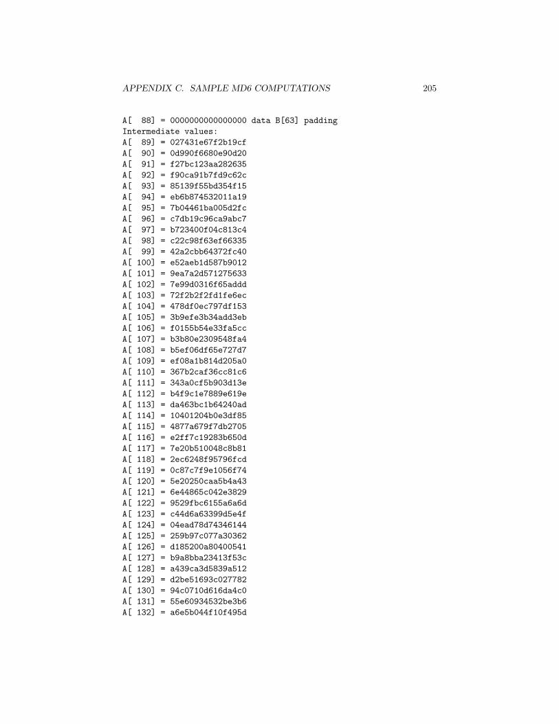
APPENDIX C. SAMPLE MD6 COMPUTATIONS 205
A[ 88] = 0000000000000000 data B[63] paddingIntermediate values:A[ 89] = 027431e67f2b19cfA[ 90] = 0d990f6680e90d20A[ 91] = f27bc123aa282635A[ 92] = f90ca91b7fd9c62cA[ 93] = 85139f55bd354f15A[ 94] = eb6b874532011a19A[ 95] = 7b04461ba005d2fcA[ 96] = c7db19c96ca9abc7A[ 97] = b723400f04c813c4A[ 98] = c22c98f63ef66335A[ 99] = 42a2cbb64372fc40A[ 100] = e52aeb1d587b9012A[ 101] = 9ea7a2d571275633A[ 102] = 7e99d0316f65adddA[ 103] = 72f2b2f2fd1fe6ecA[ 104] = 478df0ec797df153A[ 105] = 3b9efe3b34add3ebA[ 106] = f0155b54e33fa5ccA[ 107] = b3b80e2309548fa4A[ 108] = b5ef06df65e727d7A[ 109] = ef08a1b814d205a0A[ 110] = 367b2caf36cc81c6A[ 111] = 343a0cf5b903d13eA[ 112] = b4f9c1e7889e619eA[ 113] = da463bc1b64240adA[ 114] = 10401204b0e3df85A[ 115] = 4877a679f7db2705A[ 116] = e2ff7c19283b650dA[ 117] = 7e20b510048c8b81A[ 118] = 2ec6248f95796fcdA[ 119] = 0c87c7f9e1056f74A[ 120] = 5e20250caa5b4a43A[ 121] = 6e44865c042e3829A[ 122] = 9529fbc6155a6a6dA[ 123] = c44d6a63399d5e4fA[ 124] = 04ead78d74346144A[ 125] = 259b97c077a30362A[ 126] = d185200a80400541A[ 127] = b9a8bba23413f53cA[ 128] = a439ca3d5839a512A[ 129] = d2be51693c027782A[ 130] = 94c0710d616da4c0A[ 131] = 55e60934532be3b6A[ 132] = a6e5b044f10f495d
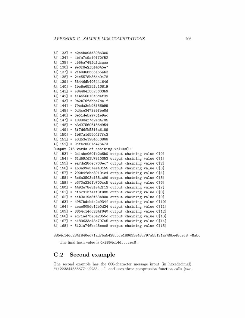
APPENDIX C. SAMPLE MD6 COMPUTATIONS 206
A[ 133] = c2a4ba0dd30863e0A[ 134] = abfa7c9a10170f52A[ 135] = c55ba748fdfdcaaaA[ 136] = 9e0f8e2fbf4645e7A[ 137] = 21b0d68b36a65ab3A[ 138] = 24e5578b36da9478A[ 139] = 58446db406441646A[ 140] = 1be8e6525fc16819A[ 141] = e84464fb02c603b9A[ 142] = a14656016a6def39A[ 143] = 9b2b76febbe7de1fA[ 144] = 79eda3eb98f56b99A[ 145] = 0d4ce347389fbe8dA[ 146] = 0e51deba9751e9acA[ 147] = a09984f7d2ed4785A[ 148] = b3d375606156d954A[ 149] = 8f7d6fb5316a6189A[ 150] = 1b87a1d5504f7fc3A[ 151] = e3d53e19846c0868A[ 152] = 9dfbc0507d476a7dOutput (16 words of chaining values):A[ 153] = 2d1abe0601b2e6b0 output chaining value C[0]A[ 154] = 61d59fd2b7310353 output chaining value C[1]A[ 155] = ea7da28dec708ec7 output chaining value C[2]A[ 156] = a63a99a574e40155 output chaining value C[3]A[ 157] = 290b4fabe80104c4 output chaining value C[4]A[ 158] = 8c6a3503cf881a99 output chaining value C[5]A[ 159] = e370e23d1b700cc5 output chaining value C[6]A[ 160] = 4492e78e3fe42f13 output chaining value C[7]A[ 161] = df6c91b7eaf3f088 output chaining value C[8]A[ 162] = aab3e19a8f63b80a output chaining value C[9]A[ 163] = d987bdcbda2e934f output chaining value C[10]A[ 164] = aeae805de12b0d24 output chaining value C[11]A[ 165] = 8854c14dc284f840 output chaining value C[12]A[ 166] = ed71ad7ba542855c output chaining value C[13]A[ 167] = e189633e48c797a5 output chaining value C[14]A[ 168] = 5121a746be48cec8 output chaining value C[15]
8854c14dc284f840ed71ad7ba542855ce189633e48c797a55121a746be48cec8 -Mabc
The final hash value is 0x8854c14d...cec8 .
C.2 Second example
The second example has the 600-character message input (in hexadecimal)“11223344556677112233...” and uses three compression function calls (two
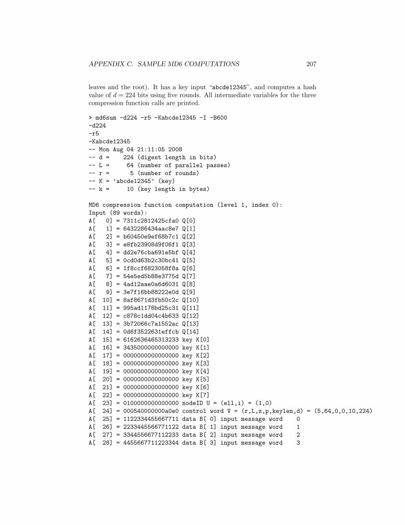
APPENDIX C. SAMPLE MD6 COMPUTATIONS 207
leaves and the root). It has a key input “abcde12345”, and computes a hashvalue of d = 224 bits using five rounds. All intermediate variables for the threecompression function calls are printed.
> md6sum -d224 -r5 -Kabcde12345 -I -B600-d224-r5-Kabcde12345-- Mon Aug 04 21:11:05 2008-- d = 224 (digest length in bits)-- L = 64 (number of parallel passes)-- r = 5 (number of rounds)-- K = ’abcde12345’ (key)-- k = 10 (key length in bytes)
MD6 compression function computation (level 1, index 0):Input (89 words):A[ 0] = 7311c2812425cfa0 Q[0]A[ 1] = 6432286434aac8e7 Q[1]A[ 2] = b60450e9ef68b7c1 Q[2]A[ 3] = e8fb23908d9f06f1 Q[3]A[ 4] = dd2e76cba691e5bf Q[4]A[ 5] = 0cd0d63b2c30bc41 Q[5]A[ 6] = 1f8ccf6823058f8a Q[6]A[ 7] = 54e5ed5b88e3775d Q[7]A[ 8] = 4ad12aae0a6d6031 Q[8]A[ 9] = 3e7f16bb88222e0d Q[9]A[ 10] = 8af8671d3fb50c2c Q[10]A[ 11] = 995ad1178bd25c31 Q[11]A[ 12] = c878c1dd04c4b633 Q[12]A[ 13] = 3b72066c7a1552ac Q[13]A[ 14] = 0d6f3522631effcb Q[14]A[ 15] = 6162636465313233 key K[0]A[ 16] = 3435000000000000 key K[1]A[ 17] = 0000000000000000 key K[2]A[ 18] = 0000000000000000 key K[3]A[ 19] = 0000000000000000 key K[4]A[ 20] = 0000000000000000 key K[5]A[ 21] = 0000000000000000 key K[6]A[ 22] = 0000000000000000 key K[7]A[ 23] = 0100000000000000 nodeID U = (ell,i) = (1,0)A[ 24] = 000540000000a0e0 control word V = (r,L,z,p,keylen,d) = (5,64,0,0,10,224)A[ 25] = 1122334455667711 data B[ 0] input message word 0A[ 26] = 2233445566771122 data B[ 1] input message word 1A[ 27] = 3344556677112233 data B[ 2] input message word 2A[ 28] = 4455667711223344 data B[ 3] input message word 3
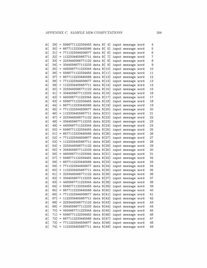
APPENDIX C. SAMPLE MD6 COMPUTATIONS 208
A[ 29] = 5566771122334455 data B[ 4] input message word 4A[ 30] = 6677112233445566 data B[ 5] input message word 5A[ 31] = 7711223344556677 data B[ 6] input message word 6A[ 32] = 1122334455667711 data B[ 7] input message word 7A[ 33] = 2233445566771122 data B[ 8] input message word 8A[ 34] = 3344556677112233 data B[ 9] input message word 9A[ 35] = 4455667711223344 data B[10] input message word 10A[ 36] = 5566771122334455 data B[11] input message word 11A[ 37] = 6677112233445566 data B[12] input message word 12A[ 38] = 7711223344556677 data B[13] input message word 13A[ 39] = 1122334455667711 data B[14] input message word 14A[ 40] = 2233445566771122 data B[15] input message word 15A[ 41] = 3344556677112233 data B[16] input message word 16A[ 42] = 4455667711223344 data B[17] input message word 17A[ 43] = 5566771122334455 data B[18] input message word 18A[ 44] = 6677112233445566 data B[19] input message word 19A[ 45] = 7711223344556677 data B[20] input message word 20A[ 46] = 1122334455667711 data B[21] input message word 21A[ 47] = 2233445566771122 data B[22] input message word 22A[ 48] = 3344556677112233 data B[23] input message word 23A[ 49] = 4455667711223344 data B[24] input message word 24A[ 50] = 5566771122334455 data B[25] input message word 25A[ 51] = 6677112233445566 data B[26] input message word 26A[ 52] = 7711223344556677 data B[27] input message word 27A[ 53] = 1122334455667711 data B[28] input message word 28A[ 54] = 2233445566771122 data B[29] input message word 29A[ 55] = 3344556677112233 data B[30] input message word 30A[ 56] = 4455667711223344 data B[31] input message word 31A[ 57] = 5566771122334455 data B[32] input message word 32A[ 58] = 6677112233445566 data B[33] input message word 33A[ 59] = 7711223344556677 data B[34] input message word 34A[ 60] = 1122334455667711 data B[35] input message word 35A[ 61] = 2233445566771122 data B[36] input message word 36A[ 62] = 3344556677112233 data B[37] input message word 37A[ 63] = 4455667711223344 data B[38] input message word 38A[ 64] = 5566771122334455 data B[39] input message word 39A[ 65] = 6677112233445566 data B[40] input message word 40A[ 66] = 7711223344556677 data B[41] input message word 41A[ 67] = 1122334455667711 data B[42] input message word 42A[ 68] = 2233445566771122 data B[43] input message word 43A[ 69] = 3344556677112233 data B[44] input message word 44A[ 70] = 4455667711223344 data B[45] input message word 45A[ 71] = 5566771122334455 data B[46] input message word 46A[ 72] = 6677112233445566 data B[47] input message word 47A[ 73] = 7711223344556677 data B[48] input message word 48A[ 74] = 1122334455667711 data B[49] input message word 49
APPENDIX C. SAMPLE MD6 COMPUTATIONS 209
A[ 75] = 2233445566771122 data B[50] input message word 50A[ 76] = 3344556677112233 data B[51] input message word 51A[ 77] = 4455667711223344 data B[52] input message word 52A[ 78] = 5566771122334455 data B[53] input message word 53A[ 79] = 6677112233445566 data B[54] input message word 54A[ 80] = 7711223344556677 data B[55] input message word 55A[ 81] = 1122334455667711 data B[56] input message word 56A[ 82] = 2233445566771122 data B[57] input message word 57A[ 83] = 3344556677112233 data B[58] input message word 58A[ 84] = 4455667711223344 data B[59] input message word 59A[ 85] = 5566771122334455 data B[60] input message word 60A[ 86] = 6677112233445566 data B[61] input message word 61A[ 87] = 7711223344556677 data B[62] input message word 62A[ 88] = 1122334455667711 data B[63] input message word 63Intermediate values:A[ 89] = 023bc36dbadd897cA[ 90] = d2927a221b06c047A[ 91] = c43ba671cd483453A[ 92] = 71fff4ac51400eceA[ 93] = 0982eb1487ed94a0A[ 94] = b0db96aa5be6e25dA[ 95] = c79104d837fa7829A[ 96] = 74f191fac63854c7A[ 97] = 555836c2482b7073A[ 98] = 96d1cfa2960a3635A[ 99] = 91f93e1e2305defbA[ 100] = a0d6fb3db7872b00A[ 101] = 09b3e3efa9f46322A[ 102] = 4f974344be9283c2A[ 103] = af945d6202a52b8aA[ 104] = 534ae6f0cc48c152A[ 105] = 9a1312a7cb95e823A[ 106] = 202d5bc69180f643A[ 107] = 3314055f3e8bd053A[ 108] = d5f43130bf23ceeaA[ 109] = 6626816602008668A[ 110] = 76aeea2aca773f6eA[ 111] = 5e85d8b579246c54A[ 112] = 2c15d20ff9b8f8c7A[ 113] = b63139c71d240633A[ 114] = f34ac4fd12d5ff52A[ 115] = e6ddcdd1c15d615eA[ 116] = 4ff6831138609787A[ 117] = 2d3f1ff4b46ae4d6A[ 118] = 0db9939d0538d1e5A[ 119] = 021d0b12738f57f8
APPENDIX C. SAMPLE MD6 COMPUTATIONS 210
A[ 120] = 225b9b9043fc1478A[ 121] = 2b44b144083caec0A[ 122] = ec7dd9746e59215aA[ 123] = 1b16f1dbf1ee2ca7A[ 124] = aff86e674d80dfc2A[ 125] = 500e4a1f3414f2e9A[ 126] = 7526f159466c0c08A[ 127] = 21872b0c3ff8f9e5A[ 128] = 9926c4c3dc26a41aA[ 129] = 1605d8571a384095A[ 130] = 36108731ac38dbbeA[ 131] = 855e83cd250610a9A[ 132] = e50d76ec2ffcd792A[ 133] = 3c25e0d2a66156b0A[ 134] = 5c0a179096bbd764A[ 135] = 69fbb852261cf3ddA[ 136] = 464e53ab124324fdA[ 137] = b82c23d382fe93b0A[ 138] = f0b2c7468873e088A[ 139] = 1617ffed131a1888A[ 140] = 4c96e83298992d59A[ 141] = 4572047f487d2c7fA[ 142] = 8dd3884af1d1fa71A[ 143] = 4e9c5579e3a882cfA[ 144] = e436a7a0b969237bA[ 145] = 4c40356771ccc066A[ 146] = c39d8cb040a1bf0fA[ 147] = 6d10e4a2236c9cc8A[ 148] = aee19ed455d9c494A[ 149] = 9beb541edf2cc926A[ 150] = 57cef68e40f3a1feA[ 151] = da808363958f463dA[ 152] = dea095fbc38c581dOutput (16 words of chaining values):A[ 153] = e86a6f805fb810ca output chaining value C[0]A[ 154] = 991de071299831a9 output chaining value C[1]A[ 155] = c59517fb7f5c5e74 output chaining value C[2]A[ 156] = 0e2b5f69481c68e6 output chaining value C[3]A[ 157] = 8ddb33a8b069b4c2 output chaining value C[4]A[ 158] = 558b3513a0046dbd output chaining value C[5]A[ 159] = e1dfb6726949ab7e output chaining value C[6]A[ 160] = f48bae515e89ee94 output chaining value C[7]A[ 161] = d31d1f87d97da302 output chaining value C[8]A[ 162] = 5d349e9b0d69b270 output chaining value C[9]A[ 163] = b409d2ee2c3e5577 output chaining value C[10]A[ 164] = 997621d403cd954e output chaining value C[11]
APPENDIX C. SAMPLE MD6 COMPUTATIONS 211
A[ 165] = 7a353e0ef29490a3 output chaining value C[12]A[ 166] = 716d1239dfff51dc output chaining value C[13]A[ 167] = 59744be898cf7c0a output chaining value C[14]A[ 168] = 07951a90e19da429 output chaining value C[15]
MD6 compression function computation (level 1, index 1):Input (89 words):A[ 0] = 7311c2812425cfa0 Q[0]A[ 1] = 6432286434aac8e7 Q[1]A[ 2] = b60450e9ef68b7c1 Q[2]A[ 3] = e8fb23908d9f06f1 Q[3]A[ 4] = dd2e76cba691e5bf Q[4]A[ 5] = 0cd0d63b2c30bc41 Q[5]A[ 6] = 1f8ccf6823058f8a Q[6]A[ 7] = 54e5ed5b88e3775d Q[7]A[ 8] = 4ad12aae0a6d6031 Q[8]A[ 9] = 3e7f16bb88222e0d Q[9]A[ 10] = 8af8671d3fb50c2c Q[10]A[ 11] = 995ad1178bd25c31 Q[11]A[ 12] = c878c1dd04c4b633 Q[12]A[ 13] = 3b72066c7a1552ac Q[13]A[ 14] = 0d6f3522631effcb Q[14]A[ 15] = 6162636465313233 key K[0]A[ 16] = 3435000000000000 key K[1]A[ 17] = 0000000000000000 key K[2]A[ 18] = 0000000000000000 key K[3]A[ 19] = 0000000000000000 key K[4]A[ 20] = 0000000000000000 key K[5]A[ 21] = 0000000000000000 key K[6]A[ 22] = 0000000000000000 key K[7]A[ 23] = 0100000000000001 nodeID U = (ell,i) = (1,1)A[ 24] = 00054000d400a0e0 control word V = (r,L,z,p,keylen,d) = (5,64,0,3392,10,224)A[ 25] = 2233445566771122 data B[ 0] input message word 64A[ 26] = 3344556677112233 data B[ 1] input message word 65A[ 27] = 4455667711223344 data B[ 2] input message word 66A[ 28] = 5566771122334455 data B[ 3] input message word 67A[ 29] = 6677112233445566 data B[ 4] input message word 68A[ 30] = 7711223344556677 data B[ 5] input message word 69A[ 31] = 1122334455667711 data B[ 6] input message word 70A[ 32] = 2233445566771122 data B[ 7] input message word 71A[ 33] = 3344556677112233 data B[ 8] input message word 72A[ 34] = 4455667711223344 data B[ 9] input message word 73A[ 35] = 5566771122334455 data B[10] input message word 74A[ 36] = 0000000000000000 data B[11] paddingA[ 37] = 0000000000000000 data B[12] paddingA[ 38] = 0000000000000000 data B[13] padding
APPENDIX C. SAMPLE MD6 COMPUTATIONS 212
A[ 39] = 0000000000000000 data B[14] paddingA[ 40] = 0000000000000000 data B[15] paddingA[ 41] = 0000000000000000 data B[16] paddingA[ 42] = 0000000000000000 data B[17] paddingA[ 43] = 0000000000000000 data B[18] paddingA[ 44] = 0000000000000000 data B[19] paddingA[ 45] = 0000000000000000 data B[20] paddingA[ 46] = 0000000000000000 data B[21] paddingA[ 47] = 0000000000000000 data B[22] paddingA[ 48] = 0000000000000000 data B[23] paddingA[ 49] = 0000000000000000 data B[24] paddingA[ 50] = 0000000000000000 data B[25] paddingA[ 51] = 0000000000000000 data B[26] paddingA[ 52] = 0000000000000000 data B[27] paddingA[ 53] = 0000000000000000 data B[28] paddingA[ 54] = 0000000000000000 data B[29] paddingA[ 55] = 0000000000000000 data B[30] paddingA[ 56] = 0000000000000000 data B[31] paddingA[ 57] = 0000000000000000 data B[32] paddingA[ 58] = 0000000000000000 data B[33] paddingA[ 59] = 0000000000000000 data B[34] paddingA[ 60] = 0000000000000000 data B[35] paddingA[ 61] = 0000000000000000 data B[36] paddingA[ 62] = 0000000000000000 data B[37] paddingA[ 63] = 0000000000000000 data B[38] paddingA[ 64] = 0000000000000000 data B[39] paddingA[ 65] = 0000000000000000 data B[40] paddingA[ 66] = 0000000000000000 data B[41] paddingA[ 67] = 0000000000000000 data B[42] paddingA[ 68] = 0000000000000000 data B[43] paddingA[ 69] = 0000000000000000 data B[44] paddingA[ 70] = 0000000000000000 data B[45] paddingA[ 71] = 0000000000000000 data B[46] paddingA[ 72] = 0000000000000000 data B[47] paddingA[ 73] = 0000000000000000 data B[48] paddingA[ 74] = 0000000000000000 data B[49] paddingA[ 75] = 0000000000000000 data B[50] paddingA[ 76] = 0000000000000000 data B[51] paddingA[ 77] = 0000000000000000 data B[52] paddingA[ 78] = 0000000000000000 data B[53] paddingA[ 79] = 0000000000000000 data B[54] paddingA[ 80] = 0000000000000000 data B[55] paddingA[ 81] = 0000000000000000 data B[56] paddingA[ 82] = 0000000000000000 data B[57] paddingA[ 83] = 0000000000000000 data B[58] paddingA[ 84] = 0000000000000000 data B[59] padding
APPENDIX C. SAMPLE MD6 COMPUTATIONS 213
A[ 85] = 0000000000000000 data B[60] paddingA[ 86] = 0000000000000000 data B[61] paddingA[ 87] = 0000000000000000 data B[62] paddingA[ 88] = 0000000000000000 data B[63] paddingIntermediate values:A[ 89] = 027431e67f2b19cfA[ 90] = 0d990f6680e90d20A[ 91] = f27bc123aa282635A[ 92] = f90ca91b7fd9c62cA[ 93] = 85139f55bd354f15A[ 94] = eb6b874532011a19A[ 95] = 7b04461ba005d2fcA[ 96] = c7db19c96ca9abc7A[ 97] = b723400f04c813c4A[ 98] = c22c98f63ef66335A[ 99] = 42a2cbb64372fc40A[ 100] = e52aeb1d587b9012A[ 101] = 9ea7a2d571275633A[ 102] = 7e99d0316f65adddA[ 103] = 72f2b2f2fd1fe6ecA[ 104] = ee030108c4c8d073A[ 105] = cfccf37b34add3ebA[ 106] = f0155b54e33fa5ccA[ 107] = b3b80e2309548fa4A[ 108] = b5ef06df65e727d7A[ 109] = ef08a1b814d205a0A[ 110] = 367b2caf36cc81c6A[ 111] = 343a0cf5b903d13eA[ 112] = b4f9c1e7889ee19fA[ 113] = da463fdb2c80b3cfA[ 114] = 5e57342f3b497579A[ 115] = ec2a9bbbac242772A[ 116] = f1ece4e7901b8a58A[ 117] = 46a38ec4458509bcA[ 118] = 9f023b8106000b81A[ 119] = bee8b8b568415c9aA[ 120] = 0941caa98d3a8735A[ 121] = 1f0d393d159e88a7A[ 122] = fd918160425fe96eA[ 123] = 7dc1367a2e734e1aA[ 124] = 7f151f7a5acba9c0A[ 125] = 9c97a06aeb6620c2A[ 126] = f74ca0e2c4400541A[ 127] = b9a8bba23413f53cA[ 128] = a439ca3d5839a512A[ 129] = d2be51693c22f741
APPENDIX C. SAMPLE MD6 COMPUTATIONS 214
A[ 130] = 94c0657db84579bbA[ 131] = a0261aaca9731c5fA[ 132] = 4c9411c30ffbf9faA[ 133] = 4dcf01f6386f9b7eA[ 134] = dbaaf2cbe4f486aaA[ 135] = 7d5a36c9454ec7e4A[ 136] = f8634c771236a7ddA[ 137] = 78c3c019f44632b1A[ 138] = 6cea1a934cc7ea1eA[ 139] = fcaa77298206c0a0A[ 140] = 465b12166eccf1eeA[ 141] = c07d7163bcd05dfeA[ 142] = 841dd2066df5d2a1A[ 143] = db122831fc72f4b5A[ 144] = 08f24baf1c9d6bd8A[ 145] = 5eff0d4698d0fc06A[ 146] = 2e7d9462fae63e2cA[ 147] = bf86d1573e7fcb05A[ 148] = 81b9602f09b1b144A[ 149] = f7d0e892806029acA[ 150] = ee671dbe2f9e706cA[ 151] = 03d9c6acabf402aaA[ 152] = 2017d423651b402bOutput (16 words of chaining values):A[ 153] = 34e06cf8e7e380b8 output chaining value C[0]A[ 154] = f8736f4357f99cb8 output chaining value C[1]A[ 155] = a3e1187da8fbd4e8 output chaining value C[2]A[ 156] = 6c11da3b93aca37a output chaining value C[3]A[ 157] = 5fdb88a98301b016 output chaining value C[4]A[ 158] = 5d2a34ccc621594d output chaining value C[5]A[ 159] = d10521d7588ce414 output chaining value C[6]A[ 160] = 5040286fe773a8c0 output chaining value C[7]A[ 161] = fe030f559c8a0f0b output chaining value C[8]A[ 162] = ca289a3c963dd24b output chaining value C[9]A[ 163] = acdccf24c7a70e53 output chaining value C[10]A[ 164] = 1f451b9a0209f583 output chaining value C[11]A[ 165] = da56f65e3205064d output chaining value C[12]A[ 166] = a00e879eae6d8241 output chaining value C[13]A[ 167] = 2a2a15bc29dc56a4 output chaining value C[14]A[ 168] = 5d8e677905657f39 output chaining value C[15]
MD6 compression function computation (level 2, index 0):Input (89 words):A[ 0] = 7311c2812425cfa0 Q[0]A[ 1] = 6432286434aac8e7 Q[1]A[ 2] = b60450e9ef68b7c1 Q[2]
APPENDIX C. SAMPLE MD6 COMPUTATIONS 215
A[ 3] = e8fb23908d9f06f1 Q[3]A[ 4] = dd2e76cba691e5bf Q[4]A[ 5] = 0cd0d63b2c30bc41 Q[5]A[ 6] = 1f8ccf6823058f8a Q[6]A[ 7] = 54e5ed5b88e3775d Q[7]A[ 8] = 4ad12aae0a6d6031 Q[8]A[ 9] = 3e7f16bb88222e0d Q[9]A[ 10] = 8af8671d3fb50c2c Q[10]A[ 11] = 995ad1178bd25c31 Q[11]A[ 12] = c878c1dd04c4b633 Q[12]A[ 13] = 3b72066c7a1552ac Q[13]A[ 14] = 0d6f3522631effcb Q[14]A[ 15] = 6162636465313233 key K[0]A[ 16] = 3435000000000000 key K[1]A[ 17] = 0000000000000000 key K[2]A[ 18] = 0000000000000000 key K[3]A[ 19] = 0000000000000000 key K[4]A[ 20] = 0000000000000000 key K[5]A[ 21] = 0000000000000000 key K[6]A[ 22] = 0000000000000000 key K[7]A[ 23] = 0200000000000000 nodeID U = (ell,i) = (2,0)A[ 24] = 000540108000a0e0 control word V = (r,L,z,p,keylen,d) = (5,64,1,2048,10,224)A[ 25] = e86a6f805fb810ca data B[ 0] chaining from (1,0)A[ 26] = 991de071299831a9 data B[ 1] chaining from (1,0)A[ 27] = c59517fb7f5c5e74 data B[ 2] chaining from (1,0)A[ 28] = 0e2b5f69481c68e6 data B[ 3] chaining from (1,0)A[ 29] = 8ddb33a8b069b4c2 data B[ 4] chaining from (1,0)A[ 30] = 558b3513a0046dbd data B[ 5] chaining from (1,0)A[ 31] = e1dfb6726949ab7e data B[ 6] chaining from (1,0)A[ 32] = f48bae515e89ee94 data B[ 7] chaining from (1,0)A[ 33] = d31d1f87d97da302 data B[ 8] chaining from (1,0)A[ 34] = 5d349e9b0d69b270 data B[ 9] chaining from (1,0)A[ 35] = b409d2ee2c3e5577 data B[10] chaining from (1,0)A[ 36] = 997621d403cd954e data B[11] chaining from (1,0)A[ 37] = 7a353e0ef29490a3 data B[12] chaining from (1,0)A[ 38] = 716d1239dfff51dc data B[13] chaining from (1,0)A[ 39] = 59744be898cf7c0a data B[14] chaining from (1,0)A[ 40] = 07951a90e19da429 data B[15] chaining from (1,0)A[ 41] = 34e06cf8e7e380b8 data B[16] chaining from (1,1)A[ 42] = f8736f4357f99cb8 data B[17] chaining from (1,1)A[ 43] = a3e1187da8fbd4e8 data B[18] chaining from (1,1)A[ 44] = 6c11da3b93aca37a data B[19] chaining from (1,1)A[ 45] = 5fdb88a98301b016 data B[20] chaining from (1,1)A[ 46] = 5d2a34ccc621594d data B[21] chaining from (1,1)A[ 47] = d10521d7588ce414 data B[22] chaining from (1,1)A[ 48] = 5040286fe773a8c0 data B[23] chaining from (1,1)
APPENDIX C. SAMPLE MD6 COMPUTATIONS 216
A[ 49] = fe030f559c8a0f0b data B[24] chaining from (1,1)A[ 50] = ca289a3c963dd24b data B[25] chaining from (1,1)A[ 51] = acdccf24c7a70e53 data B[26] chaining from (1,1)A[ 52] = 1f451b9a0209f583 data B[27] chaining from (1,1)A[ 53] = da56f65e3205064d data B[28] chaining from (1,1)A[ 54] = a00e879eae6d8241 data B[29] chaining from (1,1)A[ 55] = 2a2a15bc29dc56a4 data B[30] chaining from (1,1)A[ 56] = 5d8e677905657f39 data B[31] chaining from (1,1)A[ 57] = 0000000000000000 data B[32] paddingA[ 58] = 0000000000000000 data B[33] paddingA[ 59] = 0000000000000000 data B[34] paddingA[ 60] = 0000000000000000 data B[35] paddingA[ 61] = 0000000000000000 data B[36] paddingA[ 62] = 0000000000000000 data B[37] paddingA[ 63] = 0000000000000000 data B[38] paddingA[ 64] = 0000000000000000 data B[39] paddingA[ 65] = 0000000000000000 data B[40] paddingA[ 66] = 0000000000000000 data B[41] paddingA[ 67] = 0000000000000000 data B[42] paddingA[ 68] = 0000000000000000 data B[43] paddingA[ 69] = 0000000000000000 data B[44] paddingA[ 70] = 0000000000000000 data B[45] paddingA[ 71] = 0000000000000000 data B[46] paddingA[ 72] = 0000000000000000 data B[47] paddingA[ 73] = 0000000000000000 data B[48] paddingA[ 74] = 0000000000000000 data B[49] paddingA[ 75] = 0000000000000000 data B[50] paddingA[ 76] = 0000000000000000 data B[51] paddingA[ 77] = 0000000000000000 data B[52] paddingA[ 78] = 0000000000000000 data B[53] paddingA[ 79] = 0000000000000000 data B[54] paddingA[ 80] = 0000000000000000 data B[55] paddingA[ 81] = 0000000000000000 data B[56] paddingA[ 82] = 0000000000000000 data B[57] paddingA[ 83] = 0000000000000000 data B[58] paddingA[ 84] = 0000000000000000 data B[59] paddingA[ 85] = 0000000000000000 data B[60] paddingA[ 86] = 0000000000000000 data B[61] paddingA[ 87] = 0000000000000000 data B[62] paddingA[ 88] = 0000000000000000 data B[63] paddingIntermediate values:A[ 89] = 027431e67f2b19cfA[ 90] = 0d990f6680e90d20A[ 91] = f27bc123aa282635A[ 92] = f90ca91b7fd9c62cA[ 93] = 85139f55bd354f15
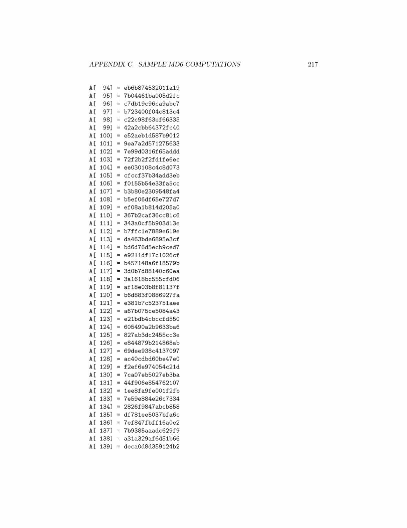
APPENDIX C. SAMPLE MD6 COMPUTATIONS 217
A[ 94] = eb6b874532011a19A[ 95] = 7b04461ba005d2fcA[ 96] = c7db19c96ca9abc7A[ 97] = b723400f04c813c4A[ 98] = c22c98f63ef66335A[ 99] = 42a2cbb64372fc40A[ 100] = e52aeb1d587b9012A[ 101] = 9ea7a2d571275633A[ 102] = 7e99d0316f65adddA[ 103] = 72f2b2f2fd1fe6ecA[ 104] = ee030108c4c8d073A[ 105] = cfccf37b34add3ebA[ 106] = f0155b54e33fa5ccA[ 107] = b3b80e2309548fa4A[ 108] = b5ef06df65e727d7A[ 109] = ef08a1b814d205a0A[ 110] = 367b2caf36cc81c6A[ 111] = 343a0cf5b903d13eA[ 112] = b7ffc1e7889e619eA[ 113] = da463bde6895e3cfA[ 114] = bd6d76d5ecb9ced7A[ 115] = e9211df17c1026cfA[ 116] = b457148a6f18579bA[ 117] = 3d0b7d88140c60eaA[ 118] = 3a1618bc555cfd06A[ 119] = af18e03b8f81137fA[ 120] = b6d883f0886927faA[ 121] = e381b7c523751aeeA[ 122] = a67b075ce5084a43A[ 123] = e21bdb4cbccfd550A[ 124] = 605490a2b9633ba6A[ 125] = 827ab3dc2455cc3eA[ 126] = e844879b214868abA[ 127] = 69dee938c4137097A[ 128] = ac40cdbd60be47e0A[ 129] = f2ef6e974054c21dA[ 130] = 7ca07eb5027eb3baA[ 131] = 44f906e854762107A[ 132] = 1ee8fa9fe001f2fbA[ 133] = 7e59e884e26c7334A[ 134] = 2826f9847abcb858A[ 135] = df781ee5037bfa6cA[ 136] = 7ef847fbff16a0e2A[ 137] = 7b9385aaadc629f9A[ 138] = a31a329af6d51b66A[ 139] = deca0d8d359124b2
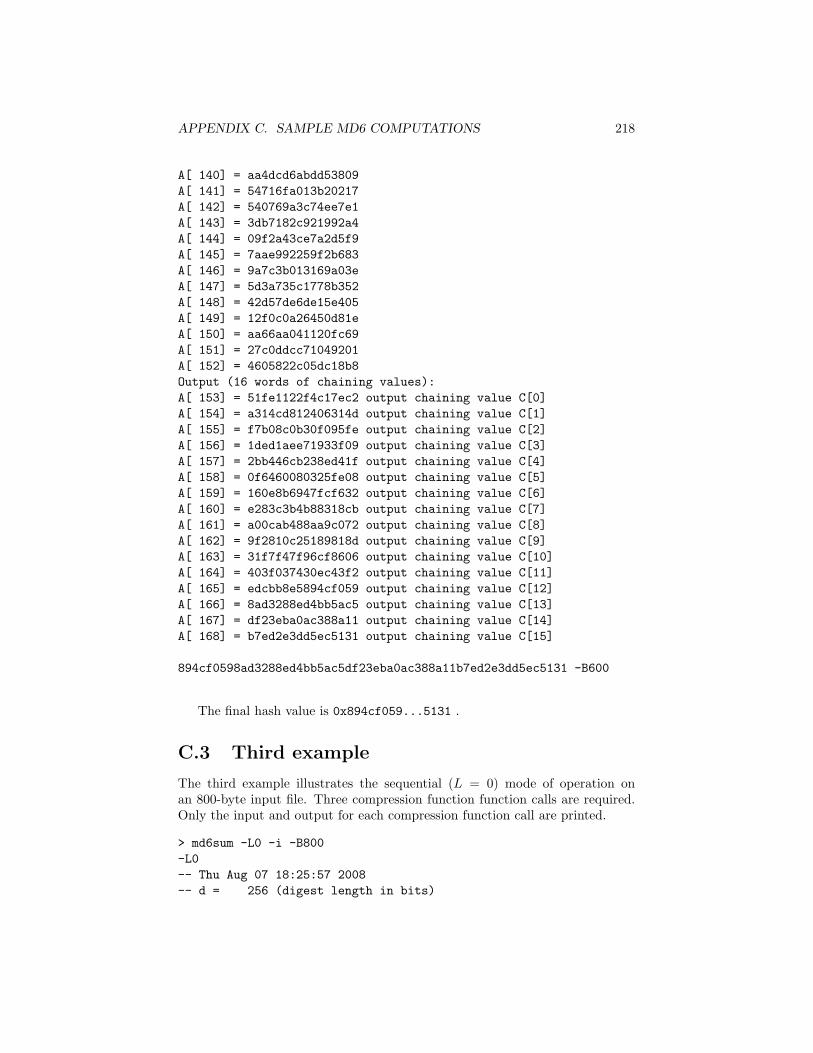
APPENDIX C. SAMPLE MD6 COMPUTATIONS 218
A[ 140] = aa4dcd6abdd53809A[ 141] = 54716fa013b20217A[ 142] = 540769a3c74ee7e1A[ 143] = 3db7182c921992a4A[ 144] = 09f2a43ce7a2d5f9A[ 145] = 7aae992259f2b683A[ 146] = 9a7c3b013169a03eA[ 147] = 5d3a735c1778b352A[ 148] = 42d57de6de15e405A[ 149] = 12f0c0a26450d81eA[ 150] = aa66aa041120fc69A[ 151] = 27c0ddcc71049201A[ 152] = 4605822c05dc18b8Output (16 words of chaining values):A[ 153] = 51fe1122f4c17ec2 output chaining value C[0]A[ 154] = a314cd812406314d output chaining value C[1]A[ 155] = f7b08c0b30f095fe output chaining value C[2]A[ 156] = 1ded1aee71933f09 output chaining value C[3]A[ 157] = 2bb446cb238ed41f output chaining value C[4]A[ 158] = 0f6460080325fe08 output chaining value C[5]A[ 159] = 160e8b6947fcf632 output chaining value C[6]A[ 160] = e283c3b4b88318cb output chaining value C[7]A[ 161] = a00cab488aa9c072 output chaining value C[8]A[ 162] = 9f2810c25189818d output chaining value C[9]A[ 163] = 31f7f47f96cf8606 output chaining value C[10]A[ 164] = 403f037430ec43f2 output chaining value C[11]A[ 165] = edcbb8e5894cf059 output chaining value C[12]A[ 166] = 8ad3288ed4bb5ac5 output chaining value C[13]A[ 167] = df23eba0ac388a11 output chaining value C[14]A[ 168] = b7ed2e3dd5ec5131 output chaining value C[15]
894cf0598ad3288ed4bb5ac5df23eba0ac388a11b7ed2e3dd5ec5131 -B600
The final hash value is 0x894cf059...5131 .
C.3 Third example
The third example illustrates the sequential (L = 0) mode of operation onan 800-byte input file. Three compression function function calls are required.Only the input and output for each compression function call are printed.
> md6sum -L0 -i -B800-L0-- Thu Aug 07 18:25:57 2008-- d = 256 (digest length in bits)
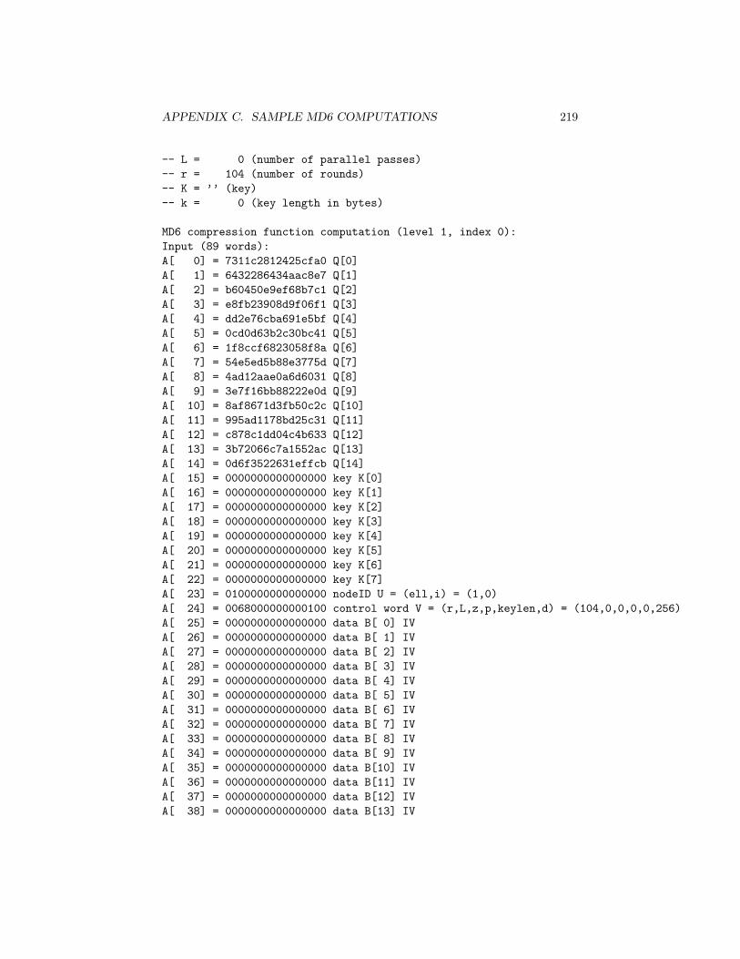
APPENDIX C. SAMPLE MD6 COMPUTATIONS 219
-- L = 0 (number of parallel passes)-- r = 104 (number of rounds)-- K = ’’ (key)-- k = 0 (key length in bytes)
MD6 compression function computation (level 1, index 0):Input (89 words):A[ 0] = 7311c2812425cfa0 Q[0]A[ 1] = 6432286434aac8e7 Q[1]A[ 2] = b60450e9ef68b7c1 Q[2]A[ 3] = e8fb23908d9f06f1 Q[3]A[ 4] = dd2e76cba691e5bf Q[4]A[ 5] = 0cd0d63b2c30bc41 Q[5]A[ 6] = 1f8ccf6823058f8a Q[6]A[ 7] = 54e5ed5b88e3775d Q[7]A[ 8] = 4ad12aae0a6d6031 Q[8]A[ 9] = 3e7f16bb88222e0d Q[9]A[ 10] = 8af8671d3fb50c2c Q[10]A[ 11] = 995ad1178bd25c31 Q[11]A[ 12] = c878c1dd04c4b633 Q[12]A[ 13] = 3b72066c7a1552ac Q[13]A[ 14] = 0d6f3522631effcb Q[14]A[ 15] = 0000000000000000 key K[0]A[ 16] = 0000000000000000 key K[1]A[ 17] = 0000000000000000 key K[2]A[ 18] = 0000000000000000 key K[3]A[ 19] = 0000000000000000 key K[4]A[ 20] = 0000000000000000 key K[5]A[ 21] = 0000000000000000 key K[6]A[ 22] = 0000000000000000 key K[7]A[ 23] = 0100000000000000 nodeID U = (ell,i) = (1,0)A[ 24] = 0068000000000100 control word V = (r,L,z,p,keylen,d) = (104,0,0,0,0,256)A[ 25] = 0000000000000000 data B[ 0] IVA[ 26] = 0000000000000000 data B[ 1] IVA[ 27] = 0000000000000000 data B[ 2] IVA[ 28] = 0000000000000000 data B[ 3] IVA[ 29] = 0000000000000000 data B[ 4] IVA[ 30] = 0000000000000000 data B[ 5] IVA[ 31] = 0000000000000000 data B[ 6] IVA[ 32] = 0000000000000000 data B[ 7] IVA[ 33] = 0000000000000000 data B[ 8] IVA[ 34] = 0000000000000000 data B[ 9] IVA[ 35] = 0000000000000000 data B[10] IVA[ 36] = 0000000000000000 data B[11] IVA[ 37] = 0000000000000000 data B[12] IVA[ 38] = 0000000000000000 data B[13] IV
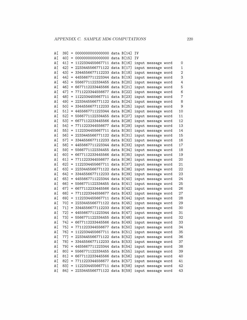
APPENDIX C. SAMPLE MD6 COMPUTATIONS 220
A[ 39] = 0000000000000000 data B[14] IVA[ 40] = 0000000000000000 data B[15] IVA[ 41] = 1122334455667711 data B[16] input message word 0A[ 42] = 2233445566771122 data B[17] input message word 1A[ 43] = 3344556677112233 data B[18] input message word 2A[ 44] = 4455667711223344 data B[19] input message word 3A[ 45] = 5566771122334455 data B[20] input message word 4A[ 46] = 6677112233445566 data B[21] input message word 5A[ 47] = 7711223344556677 data B[22] input message word 6A[ 48] = 1122334455667711 data B[23] input message word 7A[ 49] = 2233445566771122 data B[24] input message word 8A[ 50] = 3344556677112233 data B[25] input message word 9A[ 51] = 4455667711223344 data B[26] input message word 10A[ 52] = 5566771122334455 data B[27] input message word 11A[ 53] = 6677112233445566 data B[28] input message word 12A[ 54] = 7711223344556677 data B[29] input message word 13A[ 55] = 1122334455667711 data B[30] input message word 14A[ 56] = 2233445566771122 data B[31] input message word 15A[ 57] = 3344556677112233 data B[32] input message word 16A[ 58] = 4455667711223344 data B[33] input message word 17A[ 59] = 5566771122334455 data B[34] input message word 18A[ 60] = 6677112233445566 data B[35] input message word 19A[ 61] = 7711223344556677 data B[36] input message word 20A[ 62] = 1122334455667711 data B[37] input message word 21A[ 63] = 2233445566771122 data B[38] input message word 22A[ 64] = 3344556677112233 data B[39] input message word 23A[ 65] = 4455667711223344 data B[40] input message word 24A[ 66] = 5566771122334455 data B[41] input message word 25A[ 67] = 6677112233445566 data B[42] input message word 26A[ 68] = 7711223344556677 data B[43] input message word 27A[ 69] = 1122334455667711 data B[44] input message word 28A[ 70] = 2233445566771122 data B[45] input message word 29A[ 71] = 3344556677112233 data B[46] input message word 30A[ 72] = 4455667711223344 data B[47] input message word 31A[ 73] = 5566771122334455 data B[48] input message word 32A[ 74] = 6677112233445566 data B[49] input message word 33A[ 75] = 7711223344556677 data B[50] input message word 34A[ 76] = 1122334455667711 data B[51] input message word 35A[ 77] = 2233445566771122 data B[52] input message word 36A[ 78] = 3344556677112233 data B[53] input message word 37A[ 79] = 4455667711223344 data B[54] input message word 38A[ 80] = 5566771122334455 data B[55] input message word 39A[ 81] = 6677112233445566 data B[56] input message word 40A[ 82] = 7711223344556677 data B[57] input message word 41A[ 83] = 1122334455667711 data B[58] input message word 42A[ 84] = 2233445566771122 data B[59] input message word 43
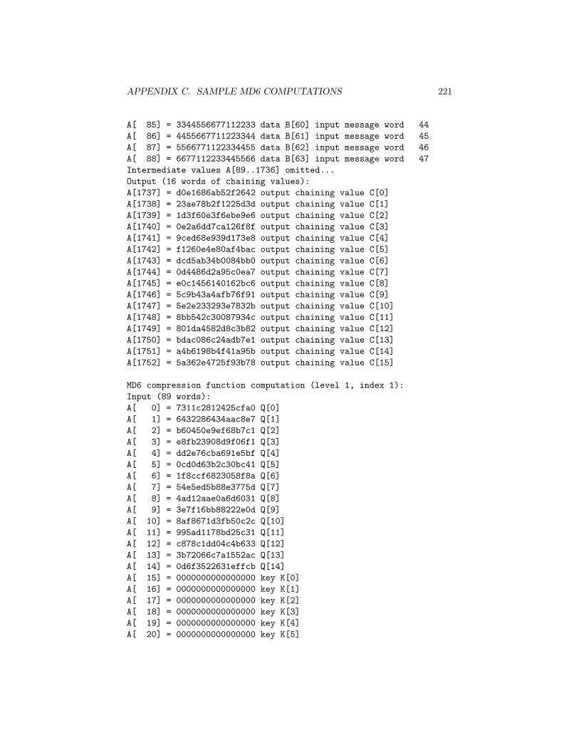
APPENDIX C. SAMPLE MD6 COMPUTATIONS 221
A[ 85] = 3344556677112233 data B[60] input message word 44A[ 86] = 4455667711223344 data B[61] input message word 45A[ 87] = 5566771122334455 data B[62] input message word 46A[ 88] = 6677112233445566 data B[63] input message word 47Intermediate values A[89..1736] omitted...Output (16 words of chaining values):A[1737] = d0e1686ab52f2642 output chaining value C[0]A[1738] = 23ae78b2f1225d3d output chaining value C[1]A[1739] = 1d3f60e3f6ebe9e6 output chaining value C[2]A[1740] = 0e2a6dd7ca126f8f output chaining value C[3]A[1741] = 9ced68e939d173e8 output chaining value C[4]A[1742] = f1260e4e80af4bac output chaining value C[5]A[1743] = dcd5ab34b0084bb0 output chaining value C[6]A[1744] = 0d4486d2a95c0ea7 output chaining value C[7]A[1745] = e0c1456140162bc6 output chaining value C[8]A[1746] = 5c9b43a4afb76f91 output chaining value C[9]A[1747] = 5e2e233293e7832b output chaining value C[10]A[1748] = 8bb542c30087934c output chaining value C[11]A[1749] = 801da4582d8c3b82 output chaining value C[12]A[1750] = bdac086c24adb7e1 output chaining value C[13]A[1751] = a4b6198b4f41a95b output chaining value C[14]A[1752] = 5a362e4725f93b78 output chaining value C[15]
MD6 compression function computation (level 1, index 1):Input (89 words):A[ 0] = 7311c2812425cfa0 Q[0]A[ 1] = 6432286434aac8e7 Q[1]A[ 2] = b60450e9ef68b7c1 Q[2]A[ 3] = e8fb23908d9f06f1 Q[3]A[ 4] = dd2e76cba691e5bf Q[4]A[ 5] = 0cd0d63b2c30bc41 Q[5]A[ 6] = 1f8ccf6823058f8a Q[6]A[ 7] = 54e5ed5b88e3775d Q[7]A[ 8] = 4ad12aae0a6d6031 Q[8]A[ 9] = 3e7f16bb88222e0d Q[9]A[ 10] = 8af8671d3fb50c2c Q[10]A[ 11] = 995ad1178bd25c31 Q[11]A[ 12] = c878c1dd04c4b633 Q[12]A[ 13] = 3b72066c7a1552ac Q[13]A[ 14] = 0d6f3522631effcb Q[14]A[ 15] = 0000000000000000 key K[0]A[ 16] = 0000000000000000 key K[1]A[ 17] = 0000000000000000 key K[2]A[ 18] = 0000000000000000 key K[3]A[ 19] = 0000000000000000 key K[4]A[ 20] = 0000000000000000 key K[5]
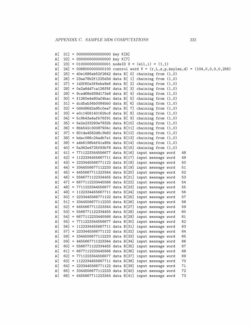
APPENDIX C. SAMPLE MD6 COMPUTATIONS 222
A[ 21] = 0000000000000000 key K[6]A[ 22] = 0000000000000000 key K[7]A[ 23] = 0100000000000001 nodeID U = (ell,i) = (1,1)A[ 24] = 0068000000000100 control word V = (r,L,z,p,keylen,d) = (104,0,0,0,0,256)A[ 25] = d0e1686ab52f2642 data B[ 0] chaining from (1,0)A[ 26] = 23ae78b2f1225d3d data B[ 1] chaining from (1,0)A[ 27] = 1d3f60e3f6ebe9e6 data B[ 2] chaining from (1,0)A[ 28] = 0e2a6dd7ca126f8f data B[ 3] chaining from (1,0)A[ 29] = 9ced68e939d173e8 data B[ 4] chaining from (1,0)A[ 30] = f1260e4e80af4bac data B[ 5] chaining from (1,0)A[ 31] = dcd5ab34b0084bb0 data B[ 6] chaining from (1,0)A[ 32] = 0d4486d2a95c0ea7 data B[ 7] chaining from (1,0)A[ 33] = e0c1456140162bc6 data B[ 8] chaining from (1,0)A[ 34] = 5c9b43a4afb76f91 data B[ 9] chaining from (1,0)A[ 35] = 5e2e233293e7832b data B[10] chaining from (1,0)A[ 36] = 8bb542c30087934c data B[11] chaining from (1,0)A[ 37] = 801da4582d8c3b82 data B[12] chaining from (1,0)A[ 38] = bdac086c24adb7e1 data B[13] chaining from (1,0)A[ 39] = a4b6198b4f41a95b data B[14] chaining from (1,0)A[ 40] = 5a362e4725f93b78 data B[15] chaining from (1,0)A[ 41] = 7711223344556677 data B[16] input message word 48A[ 42] = 1122334455667711 data B[17] input message word 49A[ 43] = 2233445566771122 data B[18] input message word 50A[ 44] = 3344556677112233 data B[19] input message word 51A[ 45] = 4455667711223344 data B[20] input message word 52A[ 46] = 5566771122334455 data B[21] input message word 53A[ 47] = 6677112233445566 data B[22] input message word 54A[ 48] = 7711223344556677 data B[23] input message word 55A[ 49] = 1122334455667711 data B[24] input message word 56A[ 50] = 2233445566771122 data B[25] input message word 57A[ 51] = 3344556677112233 data B[26] input message word 58A[ 52] = 4455667711223344 data B[27] input message word 59A[ 53] = 5566771122334455 data B[28] input message word 60A[ 54] = 6677112233445566 data B[29] input message word 61A[ 55] = 7711223344556677 data B[30] input message word 62A[ 56] = 1122334455667711 data B[31] input message word 63A[ 57] = 2233445566771122 data B[32] input message word 64A[ 58] = 3344556677112233 data B[33] input message word 65A[ 59] = 4455667711223344 data B[34] input message word 66A[ 60] = 5566771122334455 data B[35] input message word 67A[ 61] = 6677112233445566 data B[36] input message word 68A[ 62] = 7711223344556677 data B[37] input message word 69A[ 63] = 1122334455667711 data B[38] input message word 70A[ 64] = 2233445566771122 data B[39] input message word 71A[ 65] = 3344556677112233 data B[40] input message word 72A[ 66] = 4455667711223344 data B[41] input message word 73
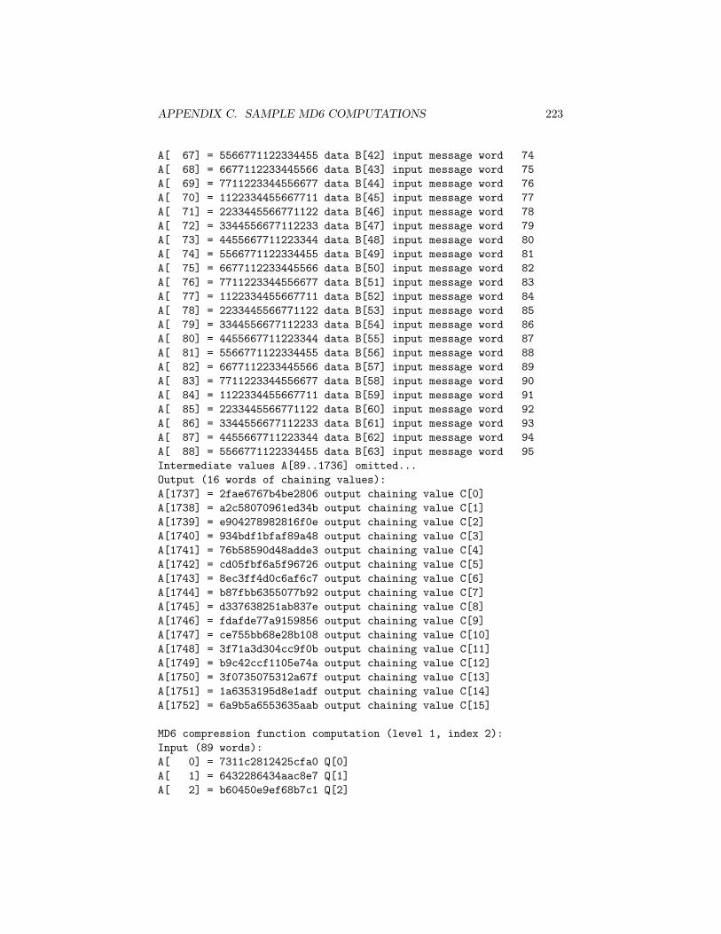
APPENDIX C. SAMPLE MD6 COMPUTATIONS 223
A[ 67] = 5566771122334455 data B[42] input message word 74A[ 68] = 6677112233445566 data B[43] input message word 75A[ 69] = 7711223344556677 data B[44] input message word 76A[ 70] = 1122334455667711 data B[45] input message word 77A[ 71] = 2233445566771122 data B[46] input message word 78A[ 72] = 3344556677112233 data B[47] input message word 79A[ 73] = 4455667711223344 data B[48] input message word 80A[ 74] = 5566771122334455 data B[49] input message word 81A[ 75] = 6677112233445566 data B[50] input message word 82A[ 76] = 7711223344556677 data B[51] input message word 83A[ 77] = 1122334455667711 data B[52] input message word 84A[ 78] = 2233445566771122 data B[53] input message word 85A[ 79] = 3344556677112233 data B[54] input message word 86A[ 80] = 4455667711223344 data B[55] input message word 87A[ 81] = 5566771122334455 data B[56] input message word 88A[ 82] = 6677112233445566 data B[57] input message word 89A[ 83] = 7711223344556677 data B[58] input message word 90A[ 84] = 1122334455667711 data B[59] input message word 91A[ 85] = 2233445566771122 data B[60] input message word 92A[ 86] = 3344556677112233 data B[61] input message word 93A[ 87] = 4455667711223344 data B[62] input message word 94A[ 88] = 5566771122334455 data B[63] input message word 95Intermediate values A[89..1736] omitted...Output (16 words of chaining values):A[1737] = 2fae6767b4be2806 output chaining value C[0]A[1738] = a2c58070961ed34b output chaining value C[1]A[1739] = e904278982816f0e output chaining value C[2]A[1740] = 934bdf1bfaf89a48 output chaining value C[3]A[1741] = 76b58590d48adde3 output chaining value C[4]A[1742] = cd05fbf6a5f96726 output chaining value C[5]A[1743] = 8ec3ff4d0c6af6c7 output chaining value C[6]A[1744] = b87fbb6355077b92 output chaining value C[7]A[1745] = d337638251ab837e output chaining value C[8]A[1746] = fdafde77a9159856 output chaining value C[9]A[1747] = ce755bb68e28b108 output chaining value C[10]A[1748] = 3f71a3d304cc9f0b output chaining value C[11]A[1749] = b9c42ccf1105e74a output chaining value C[12]A[1750] = 3f0735075312a67f output chaining value C[13]A[1751] = 1a6353195d8e1adf output chaining value C[14]A[1752] = 6a9b5a6553635aab output chaining value C[15]
MD6 compression function computation (level 1, index 2):Input (89 words):A[ 0] = 7311c2812425cfa0 Q[0]A[ 1] = 6432286434aac8e7 Q[1]A[ 2] = b60450e9ef68b7c1 Q[2]
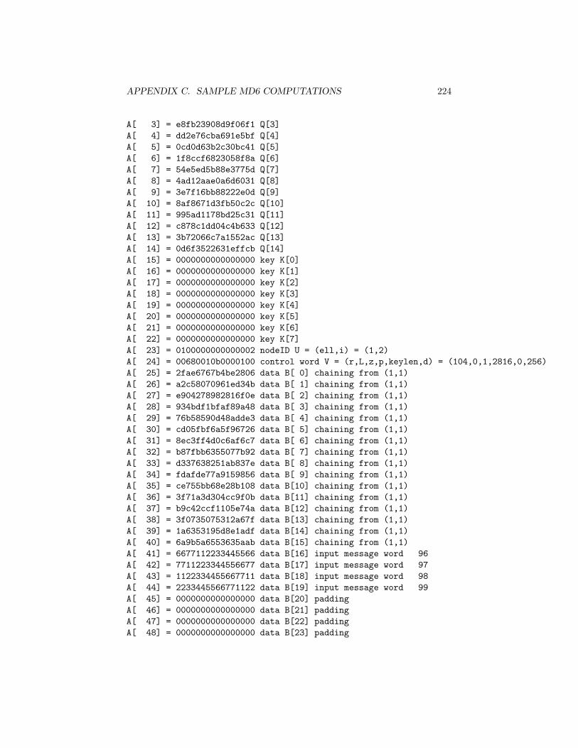
APPENDIX C. SAMPLE MD6 COMPUTATIONS 224
A[ 3] = e8fb23908d9f06f1 Q[3]A[ 4] = dd2e76cba691e5bf Q[4]A[ 5] = 0cd0d63b2c30bc41 Q[5]A[ 6] = 1f8ccf6823058f8a Q[6]A[ 7] = 54e5ed5b88e3775d Q[7]A[ 8] = 4ad12aae0a6d6031 Q[8]A[ 9] = 3e7f16bb88222e0d Q[9]A[ 10] = 8af8671d3fb50c2c Q[10]A[ 11] = 995ad1178bd25c31 Q[11]A[ 12] = c878c1dd04c4b633 Q[12]A[ 13] = 3b72066c7a1552ac Q[13]A[ 14] = 0d6f3522631effcb Q[14]A[ 15] = 0000000000000000 key K[0]A[ 16] = 0000000000000000 key K[1]A[ 17] = 0000000000000000 key K[2]A[ 18] = 0000000000000000 key K[3]A[ 19] = 0000000000000000 key K[4]A[ 20] = 0000000000000000 key K[5]A[ 21] = 0000000000000000 key K[6]A[ 22] = 0000000000000000 key K[7]A[ 23] = 0100000000000002 nodeID U = (ell,i) = (1,2)A[ 24] = 00680010b0000100 control word V = (r,L,z,p,keylen,d) = (104,0,1,2816,0,256)A[ 25] = 2fae6767b4be2806 data B[ 0] chaining from (1,1)A[ 26] = a2c58070961ed34b data B[ 1] chaining from (1,1)A[ 27] = e904278982816f0e data B[ 2] chaining from (1,1)A[ 28] = 934bdf1bfaf89a48 data B[ 3] chaining from (1,1)A[ 29] = 76b58590d48adde3 data B[ 4] chaining from (1,1)A[ 30] = cd05fbf6a5f96726 data B[ 5] chaining from (1,1)A[ 31] = 8ec3ff4d0c6af6c7 data B[ 6] chaining from (1,1)A[ 32] = b87fbb6355077b92 data B[ 7] chaining from (1,1)A[ 33] = d337638251ab837e data B[ 8] chaining from (1,1)A[ 34] = fdafde77a9159856 data B[ 9] chaining from (1,1)A[ 35] = ce755bb68e28b108 data B[10] chaining from (1,1)A[ 36] = 3f71a3d304cc9f0b data B[11] chaining from (1,1)A[ 37] = b9c42ccf1105e74a data B[12] chaining from (1,1)A[ 38] = 3f0735075312a67f data B[13] chaining from (1,1)A[ 39] = 1a6353195d8e1adf data B[14] chaining from (1,1)A[ 40] = 6a9b5a6553635aab data B[15] chaining from (1,1)A[ 41] = 6677112233445566 data B[16] input message word 96A[ 42] = 7711223344556677 data B[17] input message word 97A[ 43] = 1122334455667711 data B[18] input message word 98A[ 44] = 2233445566771122 data B[19] input message word 99A[ 45] = 0000000000000000 data B[20] paddingA[ 46] = 0000000000000000 data B[21] paddingA[ 47] = 0000000000000000 data B[22] paddingA[ 48] = 0000000000000000 data B[23] padding
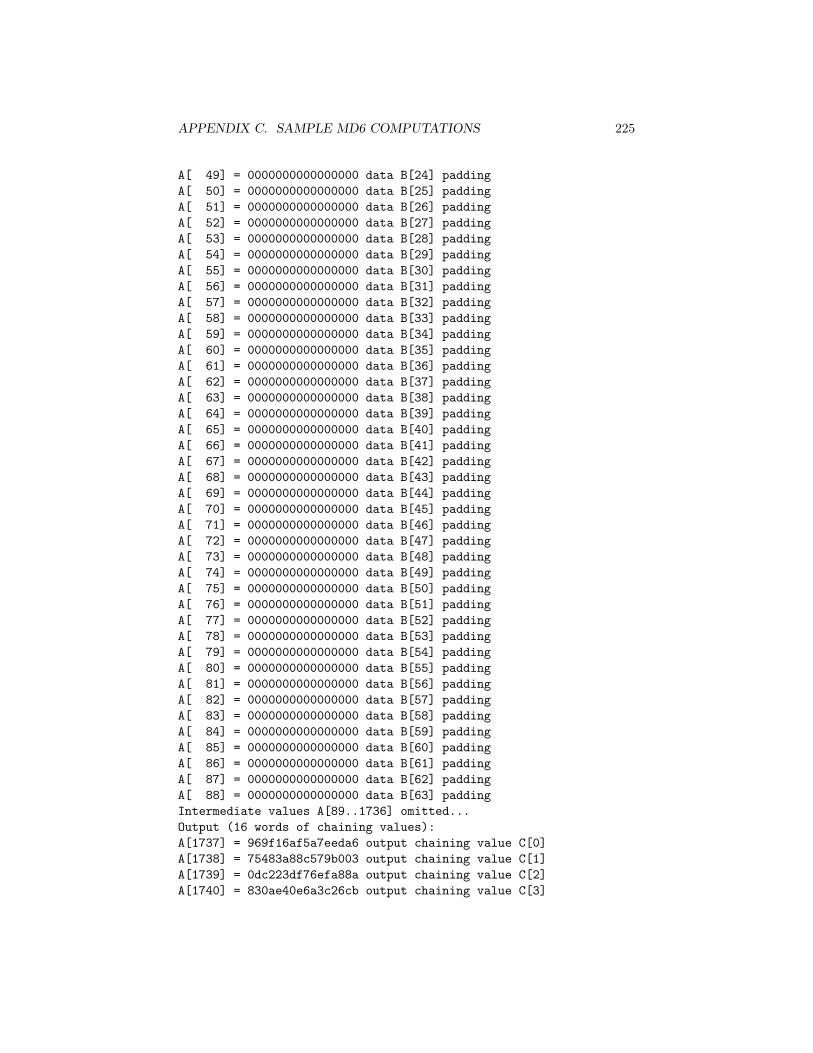
APPENDIX C. SAMPLE MD6 COMPUTATIONS 225
A[ 49] = 0000000000000000 data B[24] paddingA[ 50] = 0000000000000000 data B[25] paddingA[ 51] = 0000000000000000 data B[26] paddingA[ 52] = 0000000000000000 data B[27] paddingA[ 53] = 0000000000000000 data B[28] paddingA[ 54] = 0000000000000000 data B[29] paddingA[ 55] = 0000000000000000 data B[30] paddingA[ 56] = 0000000000000000 data B[31] paddingA[ 57] = 0000000000000000 data B[32] paddingA[ 58] = 0000000000000000 data B[33] paddingA[ 59] = 0000000000000000 data B[34] paddingA[ 60] = 0000000000000000 data B[35] paddingA[ 61] = 0000000000000000 data B[36] paddingA[ 62] = 0000000000000000 data B[37] paddingA[ 63] = 0000000000000000 data B[38] paddingA[ 64] = 0000000000000000 data B[39] paddingA[ 65] = 0000000000000000 data B[40] paddingA[ 66] = 0000000000000000 data B[41] paddingA[ 67] = 0000000000000000 data B[42] paddingA[ 68] = 0000000000000000 data B[43] paddingA[ 69] = 0000000000000000 data B[44] paddingA[ 70] = 0000000000000000 data B[45] paddingA[ 71] = 0000000000000000 data B[46] paddingA[ 72] = 0000000000000000 data B[47] paddingA[ 73] = 0000000000000000 data B[48] paddingA[ 74] = 0000000000000000 data B[49] paddingA[ 75] = 0000000000000000 data B[50] paddingA[ 76] = 0000000000000000 data B[51] paddingA[ 77] = 0000000000000000 data B[52] paddingA[ 78] = 0000000000000000 data B[53] paddingA[ 79] = 0000000000000000 data B[54] paddingA[ 80] = 0000000000000000 data B[55] paddingA[ 81] = 0000000000000000 data B[56] paddingA[ 82] = 0000000000000000 data B[57] paddingA[ 83] = 0000000000000000 data B[58] paddingA[ 84] = 0000000000000000 data B[59] paddingA[ 85] = 0000000000000000 data B[60] paddingA[ 86] = 0000000000000000 data B[61] paddingA[ 87] = 0000000000000000 data B[62] paddingA[ 88] = 0000000000000000 data B[63] paddingIntermediate values A[89..1736] omitted...Output (16 words of chaining values):A[1737] = 969f16af5a7eeda6 output chaining value C[0]A[1738] = 75483a88c579b003 output chaining value C[1]A[1739] = 0dc223df76efa88a output chaining value C[2]A[1740] = 830ae40e6a3c26cb output chaining value C[3]
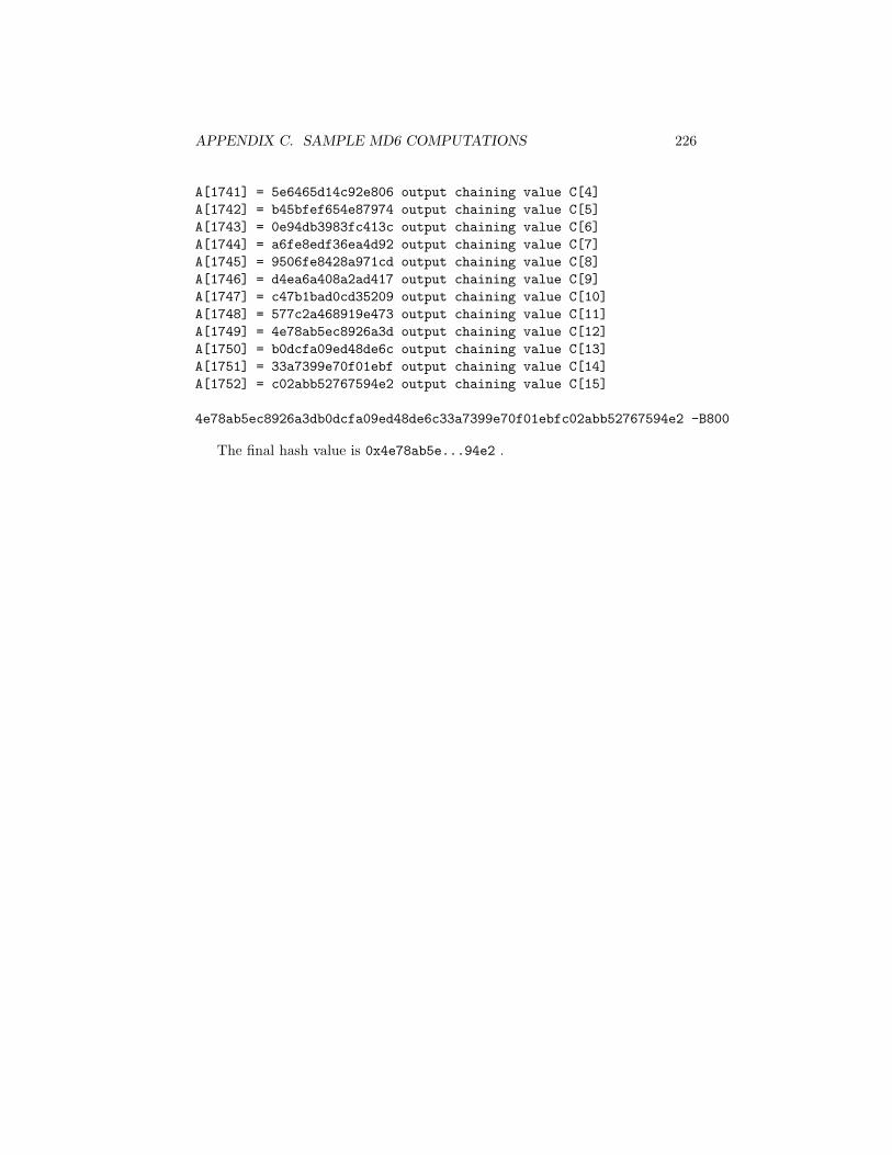
APPENDIX C. SAMPLE MD6 COMPUTATIONS 226
A[1741] = 5e6465d14c92e806 output chaining value C[4]A[1742] = b45bfef654e87974 output chaining value C[5]A[1743] = 0e94db3983fc413c output chaining value C[6]A[1744] = a6fe8edf36ea4d92 output chaining value C[7]A[1745] = 9506fe8428a971cd output chaining value C[8]A[1746] = d4ea6a408a2ad417 output chaining value C[9]A[1747] = c47b1bad0cd35209 output chaining value C[10]A[1748] = 577c2a468919e473 output chaining value C[11]A[1749] = 4e78ab5ec8926a3d output chaining value C[12]A[1750] = b0dcfa09ed48de6c output chaining value C[13]A[1751] = 33a7399e70f01ebf output chaining value C[14]A[1752] = c02abb52767594e2 output chaining value C[15]
4e78ab5ec8926a3db0dcfa09ed48de6c33a7399e70f01ebfc02abb52767594e2 -B800
The final hash value is 0x4e78ab5e...94e2 .
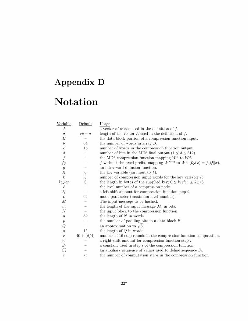
Appendix D
Notation
Variable Default UsageA – a vector of words used in the definition of f .a rc+ n length of the vector A used in the definition of f .B – the data block portion of a compression function input.b 64 the number of words in array B.c 16 number of words in the compression function output.d – number of bits in the MD6 final output (1 ≤ d ≤ 512).f – the MD6 compression function mapping Wn to W c.fQ – f without the fixed prefix, mapping Wn−q to W c: fQ(x) = f(Q||x).g – an intra-word diffusion function.K 0 the key variable (an input to f).k 8 number of compression input words for the key variable K.
keylen 0 the length in bytes of the supplied key; 0 ≤ keylen ≤ kw/8.` – the level number of a compression node.`i – a left-shift amount for compression function step i.L 64 mode parameter (maximum level number).M – The input message to be hashed.m – the length of the input message M , in bits.N – the input block to the compression function.n 89 the length of N in words.p – the number of padding bits in a data block B.Q – an approximation to
√6.
q 15 the length of Q in words.r 40 + bd/4c number of 16-step rounds in the compression function computation.ri – a right-shift amount for compression function step i.Si – a constant used in step i of the compression function.S′j – an auxiliary sequence of values used to define sequence Si.t rc the number of computation steps in the compression function.
227
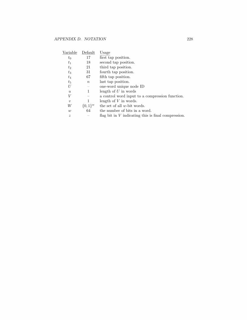
APPENDIX D. NOTATION 228
Variable Default Usaget0 17 first tap position.t1 18 second tap position.t2 21 third tap position.t3 31 fourth tap position.t4 67 fifth tap position.t5 n last tap position.U – one-word unique node IDu 1 length of U in wordsV – a control word input to a compression function.v 1 length of V in words.W {0, 1}w the set of all w-bit words.w 64 the number of bits in a word.z – flag bit in V indicating this is final compression.
Appendix E
Additional documents
This appendix describes some additional documents submitted to NIST (orpublicly available) that help to describe or illustrate the MD6 hash function.
E.1 Powerpoint slides from Rivest’s CRYPTOtalk
We have also included the Powerpoint slides from Professor Rivest’s CRYPTO2008 talk on MD6; this is file crypto2008.ppt.
E.2 Crutchfield thesis
The June 2008 MIT EECS Master’s Thesis of Christopher Crutchfield, entitled“Security Proofs for the MD6 Mode of Operation,” is included with our NISTsubmission.
E.3 Code
The MD6 Reference Implementation, Optimized 32Bit Implementation, andOptimized 64Bit implementation, are included with our NIST submission, asrequired.
Also included with our submission are the following programs:
shiftopt.c — A program used to optimize the shift amounts for MD6.
tapopt.c — A program used to optimize the tap locations for MD6.
md6sum.c — A utility program used to test MD6 and produce the intermediatevalue printouts.
229
APPENDIX E. ADDITIONAL DOCUMENTS 230
All of our software is provided under the open source “MIT License” 1, whichhas very liberal terms for copying, redistribution, modification, etc.
E.4 KAT and MCT tests
Our submission to NIST includes the KAT (Known Answer Test) and MCT(Monte Carlo Test) results as required by NIST.
There are no NIST requirements for submitting KAT or MCT test resultsfor keyed (or “salted”) versions of a submitted hash function, but Appendix Cprovides some such examples (albeit with reduced number of rounds).
E.5 One-block and two-block examples
Our submission to NIST also includes one-block and two-block examples of MD6sample computations.
These examples include the required NIST digest sizes: 224 bits, 256 bits,384 bits, and 512 bits.
For each digest size, a one-block example and a two-block example are pro-vided. The one-block examples have an input of length 400 bytes (recall thata single MD6 compression function call can handle inputs of length up to 512bytes). The “two-block” examples have an input of length 800 bytes.
For each combination of digest size and input size (one-block or two-block),there are three sample outputs provided:
• Standard MD6.
• MD6 in sequential mode (i.e., with L = 0).
• MD6 with a nine-byte key in standard mode.
Note that the “two-block” examples show three compression function calls,since in standard mode there will be two compression function calls at level 1,and one at level 2 that produces the final output, and in sequential mode the800-byte input doesn’t quite fit into two 384-byte input blocks.
E.6 Web site
We have created a web site that makes publicly available the documents we havesubmitted to NIST for the SHA-3 competition, as well as copies of (or pointersto) other documents about MD6.
This web site is available at URL:
http://groups.csail.mit.edu/cis/md6/.
1http://www.opensource.org/licenses/mit-license.php
Appendix F
MD6 team members
Here we give a little more information about each of the MD6 team members, theaspects of the MD6 development they participated in, and contact information.
(Thanks to all of the MD6 team members for their efforts!)
• Ronald L. Rivest is the lead MD6 architect and team leader. He is aProfessor in the MIT EECS Department.Web site: http://people.csail.mit.edu/rivestPhone: 617-253-5880Email: [email protected]
• Benjamin Agre is an MIT undergraduate. He worked on testing MD6using various statistical packages.Email: [email protected]
• Daniel V. Bailey studied fast embedded crypto implementation with ChristofPaar at WPI. He is now at RSA, and worked on the performance figuresfor MD6 on 8-bit processors.Email: [email protected]
• Christopher Crutchfield finished his Master’s thesis on the MD6 mode ofoperation at MIT in 2008, and is now working at a startup.Email: [email protected]
• Yevgeniy Dodis is a Professor in the Department of Computer Science atNew York University; he contributed to the proofs of security for the MD6compression function and for the MD6 mode of operation.Email: [email protected]
• Kermin Elliott Fleming is a graduate student in the Computation Struc-tures Group at MIT’s Computer Science and Artificial Intelligence Labo-ratory. He did the MD6 hardware designs reported in Chapter 5, and alsothe GPU implementation reported in Section 4.7.2.Email: [email protected]
231
APPENDIX F. MD6 TEAM MEMBERS 232
• Asif Khan is a graduate student in the Computation Structures Groupat MIT’s Computer Science and Artificial Intelligence Laboratory. Heworked on the custom multicore designs for MD6 reported in Section 5.4.Email: [email protected]
• Jayant Krishnamurthy is an MEng student in MIT’s EECS Department.He has worked on a variety of software aspects of MD6, including the“clean-room” implementation, the testing framework, efficiency optimiza-tions, and a CILK implementation.Email: [email protected]
• Yuncheng Lin graduated from MIT in 2008, and is going to graduateschool at Stanford in the Mathematics Department. He has worked onevaluating the security of MD6 against differential attack, as reported inSection 6.9.Email: [email protected]
• Leo Reyzin is a Professor of Computer Science at Boston University. Hehas worked on the security of MD6’s mode of operation.Email: [email protected] site: http://www.cs.bu.edu/~reyzin/
• Emily Shen is a graduate student in the Cryptography and InformationSecurity group in MIT’s Computer Science and Artificial Intelligence Lab-oratory. She has worked on the security of MD6’s mode of operation.Email: [email protected]
• Jim Sukha was a graduate student in Professor Leiserson’s research groupat MIT’s Computer Science and Artificial Intelligence Laboratory. Hedeveloped an initial CILK implementation of MD6.Email: [email protected]
• Drew Sutherland received his Ph.D. from the MIT Mathematics Depart-ment in 2007, on the topic of “Order Computations in Generic Groups.”Email:[email protected]
• Eran Tromer is a post-doc in the Cryptography and Information Securitygroup within MIT’s Computer Science and Artificial Intelligence Labora-tory. He has worked on a variety of aspects of MD6’s design and security,including the minisat experiments reported in Chapter 6.Email: [email protected] site: http://people.csail.mit.edu/tromer/
• Yiqun Lisa Yin received her PhD from MIT’s Mathematics Department,and is now an independent cryptography and security consultant. She hasworked on a variety of aspects of MD6’s design and security, includingdifferential cryptanalysis reported in Section 6.9 and linear cryptanalysisreported in Section 6.10.