The maximal probability that k-wise independent bits are all 1
24
The Maximal Probability That k-Wise Independent Bits Are All 1* Ron Peled, 1 Ariel Yadin, 2 Amir Yehudayoff 3 1 Courant Institute of Mathematical Sciences, New York University, New York; e-mail: [email protected] 2 Center for Mathematical Sciences, University of Cambridge, Cambridge, UK; e-mail: [email protected] 3 School of Mathematics, Institute for Advanced Study, Princeton, New Jersey; e-mail: [email protected] Received 22 July 2008; accepted 2 October 2009 Published online 25 May 2010 in Wiley Online Library (wileyonlinelibrary.com). DOI 10.1002/rsa.20329 ABSTRACT: A k-wise independent distribution on n bits is a joint distribution of the bits such that each k of them are independent. In this paper we consider k-wise independent distributions with identical marginals, each bit has probability p to be 1. We address the following question: how high can the probability that all the bits are 1 be, for such a distribution? For a wide range of the parameters n, k, and p we find an explicit lower bound for this probability which matches an upper bound given by Benjamini et al., up to multiplicative factors of lower order. In particular, for fixed k, we obtain the sharp asymptotic behavior. The question we investigate can be viewed as a relaxation of a major open problem in error-correcting codes theory, namely, how large can a linear error-correcting code with given parameters be? The question is a type of discrete moment problem, and our approach is based on showing that bounds obtained from the theory of the classical moment problem provide good approximations for it. The main tool we use is a bound controlling the change in the expectation of a polynomial after small perturbation of its zeros. © 2010 Wiley Periodicals, Inc. Random Struct. Alg., 38, 502–525, 2011 Keywords: k-wise independence; inclusion-exclusion; error correcting codes; classical moment problem; discrete moment problem 1. INTRODUCTION The problem of generalized inclusion-exclusion inequalities has been considered by many authors [3–6, 8, 11, 12, 16]. In this problem one has n events A 1 , ... , A n and the probabilities of intersections ∩ i∈S A i for all S with |S|≤ k . Given this information the goal is to bound Correspondence to: R. Peled *Supported by NSF (DMS-0605166, CCF-0832797); Microsoft Research. © 2010 Wiley Periodicals, Inc. 502
Transcript of The maximal probability that k-wise independent bits are all 1

The Maximal Probability That k -WiseIndependent Bits Are All 1*
Ron Peled,1 Ariel Yadin,2 Amir Yehudayoff3
1Courant Institute of Mathematical Sciences, New York University, New York;e-mail: [email protected]
2Center for Mathematical Sciences, University of Cambridge, Cambridge, UK;e-mail: [email protected]
3School of Mathematics, Institute for Advanced Study, Princeton, New Jersey;e-mail: [email protected]
Received 22 July 2008; accepted 2 October 2009Published online 25 May 2010 in Wiley Online Library (wileyonlinelibrary.com).DOI 10.1002/rsa.20329
ABSTRACT: A k-wise independent distribution on n bits is a joint distribution of the bits suchthat each k of them are independent. In this paper we consider k-wise independent distributions withidentical marginals, each bit has probability p to be 1. We address the following question: how highcan the probability that all the bits are 1 be, for such a distribution? For a wide range of the parametersn, k, and p we find an explicit lower bound for this probability which matches an upper bound givenby Benjamini et al., up to multiplicative factors of lower order. In particular, for fixed k, we obtainthe sharp asymptotic behavior. The question we investigate can be viewed as a relaxation of a majoropen problem in error-correcting codes theory, namely, how large can a linear error-correcting codewith given parameters be?
The question is a type of discrete moment problem, and our approach is based on showing thatbounds obtained from the theory of the classical moment problem provide good approximations forit. The main tool we use is a bound controlling the change in the expectation of a polynomial aftersmall perturbation of its zeros. © 2010 Wiley Periodicals, Inc. Random Struct. Alg., 38, 502–525, 2011
Keywords: k-wise independence; inclusion-exclusion; error correcting codes; classical momentproblem; discrete moment problem
1. INTRODUCTION
The problem of generalized inclusion-exclusion inequalities has been considered by manyauthors [3–6,8,11,12,16]. In this problem one has n events A1, . . . , An and the probabilitiesof intersections ∩i∈SAi for all S with |S| ≤ k. Given this information the goal is to bound
Correspondence to: R. Peled*Supported by NSF (DMS-0605166, CCF-0832797); Microsoft Research.© 2010 Wiley Periodicals, Inc.
502
MAXIMAL PROBABILITY FOR 1 503
the probability of ∪ni=1Ai from above and from below. The classical Bonferroni inequalities
state that the odd and even partial sums of the inclusion-exclusion formula provide suchupper and lower bounds, respectively. But in many cases these bounds are far from beingsharp, in the sense that much tighter bounds may be deduced from the same information.
In this paper we address a special case of this question. In our setting the events all haveequal probability P(Ai) = p and are k-wise independent; that is, P(∩i∈SAi) = p|S| whenever|S| ≤ k. When referring to this case we shall use a slightly different terminology and referto the events A1, . . . , An as n bits. For convenience, we consider the intersection of eventsinstead of the union, which is equivalent by de Morgan’s rules. With this terminology we areinterested in estimating the probability of the AND of the bits given that their joint distri-bution is k-wise independent with identical marginals p. Besides the simplification arisingfrom considering a particular case, this case is of special interest from several points of view.
First, k-wise independent distributions play a key role in the computer science literaturewhere they are used for derandomization (there are many references, e.g., the survey [13]).Here is an example for the use of k-wise independence in this context: Assume that a givenefficient probabilistic algorithm A works, even when the algorithm uses pairwise indepen-dent bits instead of truly independent random bits. Since there are pairwise independent dis-tributions with small support, this implies that the algorithm can be converted to an efficientdeterministic algorithm. In order to prove that A indeed works with access to only pairwiseindependent bits, one needs to show that the probabilities of certain events (that depend onA) do not change significantly when “moving” to a pairwise independent distribution.
Second, there is a strong connection between linear error-correcting codes and k-wiseindependent distributions (when p = 1
q for a prime power q). Given a linear error-correctingcode over (GF(q))n with minimal distance d, one may obtain a k-wise independent distri-bution with k = d − 1 and p = 1
q by sampling uniformly at random from the dual of thecode and replacing the resulting codeword by the indicator word of its zeros. Although bythis construction one gets only distributions with a certain structure, this is by far the mostcommon way to construct k-wise independent distributions. It gives a simple connectionbetween the size of the code C, and the probability of getting the all 1’s vector:
P[(1, . . . , 1)] = 1
|C⊥| = |C|qn
,
where the probability is over the k-wise independent distribution constructed from C, andC⊥ is the dual of C. A very basic and open question in the theory of error-correcting codes ishow large can a linear error-correcting code be, for given n, d, q ([14], see also [7]). A largecode immediately implies a large probability for the AND of the bits, hence investigatingthe maximal probability that the AND event can achieve for a given triplet n, k, p can bethought of as a relaxation of the error-correcting codes question. However, in general, thesetwo questions turn out not to be equivalent, even asymptotically in n, as an example from(“On k-wise Independent Events and Percolation”, Benjamini, Gurel-Gurevich and Peled,manuscript in preparation) shows:
(i) For every 3-wise independent distribution µ on n bits with marginal probabilities 1/3that is obtained from a linear code as (roughly) described above, µ[(1, . . . , 1)] =O( 1
n log n ) (this is a version of Roth’s theorem on 3-term arithmetic progressions for(GF(3))n, see [15].)
(ii) There exists a 3-wise independent distribution µ′ on n bits with marginal probabilities1/3 such that µ′[(1, . . . , 1)] = �( 1
n ).
Random Structures and Algorithms DOI 10.1002/rsa
504 PELED, YADIN, AND YEHUDAYOFF
An important property of the code-based constructions of k-wise independent distributionsis that such distributions have small support. The support size is important for derandomiza-tion, as discussed above. In this paper we show existence of k-wise independent distributionsthat assign large probability to (1, . . . , 1), but we do not show that they have small support.
Third, the question has intrinsic mathematical beauty. From an analytic perspective,when attempting its solution one is naturally led to discrete analogues of classical momentproblems (classical quadrature formulas). Although some investigation of such discretemoment problems exists in the literature [10 (Chapter VIII), 5, 16], they are much lessunderstood than their classical counterparts. Still, the classical theory sheds light on ourproblem and enables us to make progress on it and obtain quite precise answers. Froma more geometric standpoint, the set of k-wise independent distributions is an interestingconvex body, the structure of which we understand quite poorly. In this work we try to atleast understand the projection of this body in one specific direction.
Finally, in the case p = 12 , the maximal probability of the AND event is also the maximal
probability for any fixed string of bits (roughly, “translating” a distribution by a constantvector, does not “affect” the k-wise independence). In other words, for p = 1
2 this maximalprobability corresponds to the minimal min-entropy possible for a k-wise independentdistribution, which seems a very basic property.
This work continues a previous work (“On k-wise Independent Events and Percolation”,Benjamini, Gurel-Gurevich and Peled, manuscript in preparation) in which an (explicit)upper bound for the AND event was found (as well as some lower bounds). The upperbound was derived as a solution to a relaxed maximization problem (see Section 3) whichappears quite similar to the original problem. The similarity makes it natural to expect thatthe upper bound be quite close to the true maximal probability. Indeed, in this work weaffirm this expectation in a large regime of the parameters.
1.1. Results
Denote by M(n, k, p) the maximal probability of the AND event for a k-wise independentdistribution on n bits with marginals p. For odd k it is shown in (“On k-wise IndependentEvents and Percolation”, Benjamini, Gurel-Gurevich and Peled, manuscript in preparation)that
M(n, k, p) = pM(n − 1, k − 1, p) (k odd), (1.1)
hence it is enough to consider the case of even k. It is also shown there that
M(n, k, p) ≤ M(n, k, p), (1.2)
where M(n, k, p) is the solution to a certain maximization problem (see Section 3) andsatisfies for even k,
M(n, k, p) = pn
P(Bin(n, 1 − p) ≤ k
2
) . (1.3)
Our main result is a lower bound for M(n, k, p) matching the bound given by M(n, k, p)
up to multiplicative factors of lower order, in a large regime of the parameters. Specifically:
Theorem 1.1. There exist constants c1, c2, c3 > 0 such that the following holds. Letn ∈ N, k ∈ N even, and 0 < p < 1. Let N = np(1 − p) − 1. Assume
k ≤ c1 · N . (1.4)
Random Structures and Algorithms DOI 10.1002/rsa
MAXIMAL PROBABILITY FOR 1 505
Then,
M(n, k, p) ≥ c3
kexp
(−c2 · k
V(N/k)
)M(n, k, p), (1.5)
where V(a) = exp(√
log(a) log log(a)).
The cases where (1.4) does not hold are not covered by Theorem 1.1. Some partialresults on these cases were given by Benjamini et al. (manuscript in preparation). For thecase n(1 − p) ≤ k
2 the bound pn ≤ M(n, k, p) ≤ M(n, k, p) ≤ 2pn was shown, and for thecase (n − 1)p ≤ 1 it was shown that M(n, k, p) = pk . The case k = 2 was also solved there.
To better understand the bound given in Theorem 1.1, we present some particular casesin the following
Corollary 1.2. There exist C, c > 0 such that for all n ∈ N, k ∈ N even, and 0 < p < 1,letting N = np(1 − p) − 1 we have
1. For every m > 0, there exists N0 = N0(m) such that if N > N0 and k ≤ (log N)m,then
M(n, k, p) ≥ c
kM(n, k, p).
2. For every 0 < β < 1, there exists c(β) > 0 and N0 = N0(β) such that if N > N0 andk ≤ Nβ , then
M(n, k, p) ≥ c exp
(− k
exp(c(β)√
log(k) log log(2k))
)M(n, k, p).
3. For any k satisfying k ≤ cN,
M(n, k, p) ≥ ce−CkM(n, k, p).
By estimating M(n, k, p) [using (1.3) and Claim 4.2 below] in the first two cases of theabove corollary we obtain, using (1.2), explicit two-sided bounds on M(n, k, p). They showthat for a large range of the parameters, the leading order behavior of M(n, k, p) is identifiedand for the case of constant k, the exact asymptotics is determined, as follows:
Corollary 1.3. There exist C, c > 0 such that for all n ∈ N, k ∈ N even, and 0 < p < 1,letting N = np(1 − p) − 1 we have
1. For every m > 0, there exists N0 = N0(m) such that if N > N0 and k ≤ (log N)m,then
c√k
(pk
2e(1 − p)n
)k/2
≤ M(n, k, p) ≤ C√
k
(pk
2e(1 − p)n
)k/2
. (1.6)
2. For every 0 < β < 1, there exists c(β) > 0 and N0 = N0(β) such that if N > N0 andk ≤ Nβ , then
Random Structures and Algorithms DOI 10.1002/rsa

506 PELED, YADIN, AND YEHUDAYOFF
1
Ce− k
U(k,β)
(pk
2e(1 − p)n
)k/2
≤ M(n, k, p) ≤ C√
kek22n
(pk
2e(1 − p)n
)k/2
, (1.7)
where U(k, β)def= exp(c(β)
√log(k) log log(2k)).
Let us compare this with known results, our novelty is in the lower bounds and so we onlycompare these. As far as the authors are aware, the best known lower bounds for M(n, k, p)
come from error-correcting codes and apply to the cases when p = 1q for a prime power q.
The most important case for applications is p = 12 . In this case it was known using BCH
codes [2,14 (Chapter 15)] that M(n, k, 12 ) ≥ (
c1n )k/2 and also using the Gilbert-Varshamov
bound [14] that M(n, k, 12 ) ≥ c2(
c3(k−1)
n )k−1 for some constants c1, c2, c3 > 0. In both casesour bound improves on the known asymptotic results for k = o(n), but still growing toinfinity with n.
Other cases where lower bounds were known are the cases in which p = 1q �= 1
2 for aprime power q. In these cases much less is known and even for the case of constant k andp, the best results we are aware of are of the form M(n, k, p) ≥ n−α(k,p)(1+o(1)) where, exceptfor a few cases, α(k, p) is strictly larger than k
2 (see [7] for a survey of such results). Forexample, in the case p = 1
3 and constant k ≥ 7 it appears that the best known asymptoticresult in n was M(n, k, 1
3 ) ≥ cn−�2(k−1)/3 . Our results show that the correct asymptoticbehavior for constant k and p is M(n, k, p) = �(n−k/2).
Here is a high-level description of the proof of Theorem 1.1. We start by employing linearprogramming duality as in the work of Benjamini et al. (manuscript in preparation). Thisduality shows that M(n, k, p) is the minimum of the expectation Ef (X), where X ∼ Bin(n, p),over all polynomials f from a certain class [see (2.5)]. A similar duality shows that M(n, k, p)
is the minimum of the expectation Eg(X), where X ∼ Bin(n, p), over all polynomials gfrom a strictly smaller class than that of the first minimization problem [see (3.2)]. Thislatter minimization problem is exactly solvable using the methods of the classical momentproblem. We continue by associating to each polynomial f from the class of the first problem,a polynomial g from the class of the second problem, obtained by perturbing the roots of f .It thus follows that
M(n, k, p)
M(n, k, p)≤ max
(Eg(X)
Ef (X)
)
where the maximum ranges over all polynomials f from the class of the first problem withg being the polynomial associated to f . A bound for the RHS of the above inequality whichyields Theorem 1.1 is then given by Theorem 4.1. Our methods can be used to bound the“change” in expectation for other distributions as well (see Section 5 for more details). Suchan argument can be applied to other problems where there is a classical moment problemanalogue to discrete problems. It thus seems that Theorem 4.1 and its proof might be ofindependent interest.
1.2. Outline
Section 2 gives a more precise description of the question we consider, and explains someuseful facts about it, including the use of linear programming duality. Section 3 describesthe relaxed version of the problem with emphasis on its similarity to the original problem.Our main result is explained in Section 4 where the result on polynomials and the reduction
Random Structures and Algorithms DOI 10.1002/rsa

MAXIMAL PROBABILITY FOR 1 507
between them are described. We also do the computations needed to obtain Corollary 1.3there. Finally, Section 5 proves the result on polynomials. Some open problems are presentedin Section 6. For completeness, the appendix gives short proofs for the results of the workof Benjamini et al. (manuscript in preparation) that we use.
2. THE PROBLEM AND ITS DUAL
In this section we introduce notation for our problem and present it in more precise terms.We then continue to describe the dual of the problem, on which we shall concentrate in thefollowing sections. Let A(n, k, p) be the set of all probability distributions on {0, 1}n whichare k-wise independent and have identical marginals p. In other words, the distribution of(X1, . . . , Xn) belongs to A(n, k, p) if P(∀ i ∈ S Xi = 1) = p|S| for all S with |S| ≤ k.Thinking of A(n, k, p) as a body in R2n
, it is convex. Hence, bounding the probability ofthe event AND = {∀ 1 ≤ i ≤ n Xi = 1} under all probability distributions in A(n, k, p) isthe same as finding
M(n, k, p) = maxQ∈A(n,k,p)
Q(AND), (2.1)
m(n, k, p) = minQ∈A(n,k,p)
Q(AND). (2.2)
In the work of Benjamini et al. (manuscript in preparation) it was shown that for manychoices of the parameters n, k, p we have m(n, k, p) = 0, making the bound in this directionperhaps less useful. In this work we concentrate on estimating M.
A simplification of problems (2.1) and (2.2) is possible: Define the set
As(n, k, p) ⊆ A(n, k, p)
to be the set of symmetric distributions in A(n, k, p); that is, the joint distribution of(X1, . . . , Xn) is in As(n, k, p) if it is in A(n, k, p) and (X1, . . . , Xn) are exchangeable. Sincethe AND event is symmetric, one can show that
M(n, k, p) = maxQ∈As(n,k,p)
Q(AND), (2.3)
m(n, k, p) = minQ∈As(n,k,p)
Q(AND). (2.4)
Note further that a distribution in As(n, k, p) may be identified with the integer randomvariable S which counts the number of bits that are 1. Note that such an S has the followingproperties:
(I) S is supported on {0, 1, . . . , n}.(II) ESi = EXi for X ∼ Bin(n, p) and 1 ≤ i ≤ k.
The converse also holds (Benjamini et al., manuscript in preparation); that is,
Lemma 2.1. For each random variable S satisfying (I) and (II), there exists Q ∈As(n, k, p) such that S has the distribution of the number of bits which are 1 under Q.
Random Structures and Algorithms DOI 10.1002/rsa
508 PELED, YADIN, AND YEHUDAYOFF
Relying on Lemma 2.1, we shall henceforth identify As(n, k, p) with distributions S satis-fying (I) and (II) above. There is a short argument given below showing that the distributionS achieving the maximum in (2.3) is unique. Similar arguments are used in [10].
We can now think of problem (2.3) as a linear programming problem in n + 1 variables,namely, find the maximum of P(S = n) under the constraints P(S = i) ≥ 0 for 0 ≤ i ≤ n,∑n
i=0 P(S = i) = 1 and the linear conditions on P(S = i) given by (II) above. We shallestimate M(n, k, p) using the dual linear programming problem (Benjamini et al., manuscriptin preparation):
M(n, k, p) = minP∈Pd
k
EBin(n,p)P(X), (2.5)
where Pdk is the collection of polynomials P : R → R of degree at most k satisfying P(i) ≥ 0
for i ∈ {0, 1, . . . , n − 1} and P(n) ≥ 1 (the d in the notation stands for discrete). We shallbound M(n, k, p) from below by showing that for each P ∈ Pd
k , the above expectation is nottoo small.
Note that finding an optimal polynomial for the above problem gives more informationthan just M(n, k, p). By the theorem of complementary slackness of linear programming,if Z is the set of zeros of an optimal polynomial in (2.5) then the support of the optimaldistribution in (2.3) is contained in Z∪{n}. This can also be seen probabilistically since if P isan optimal polynomial, then EP(S) = M(n, k, p) for any S ∈ As(n, k, p) (since P is of degreeat most k). But for any P ∈ Pd
k we have EP(S) ≥ P(S = n), hence P(S = n) = M(n, k, p)
only when P(n) = 1 and all the support of S besides {n} is contained in the zero set of P.Of course once the support of the optimal S (or the zero set of an optimal polynomial) isknown, the exact probabilities of S can be found by solving a system of linear equations.This system always has a unique solution (it has a Van der Monde coefficient matrix), whichalso proves the uniqueness of the distribution of S.
Prékopa in his work ([16], see also [5]) considers in more generality the problem ofestimating P(S = n) for the class of random variables S with given first k moments (notnecessarily those of the Binomial). He does not use probabilistic language and instead writeshis work in linear programming terminology. Adapting one of his results to our situation,it reads
Theorem 2.2 (Prékopa [16, Theorem 9]). There exists an optimizing polynomial P for(2.5) of the following form. P(n) = 1 and P has k simple roots z1 < z2 < · · · < zk, allcontained in {0, 1, . . . , n − 1}. Furthermore
1. For even k, the roots come in pairs zi+1 = zi + 1 for odd 1 ≤ i ≤ k − 1.2. For odd k, z1 = 0 and the rest of the roots come in pairs zi+1 = zi + 1 for even
2 ≤ i ≤ k − 1.
This result is also essentially contained in [10 (Chapter VIII, Sec. 3)]. Figures 1 and 2below present such optimizing polynomials for some choices of the parameters. The theoremis not so surprising when one recalls that we are trying to minimize the expectation of Punder the positivity constraints of the class Pd
k . The theorem is valid in the generality ofPrékopa’s work, i.e., the first k moments of S are given but they do not necessarily equalthose of a Binomial random variable.
Random Structures and Algorithms DOI 10.1002/rsa

MAXIMAL PROBABILITY FOR 1 509
Fig. 1. Optimizing polynomial in (2.5) for n = 20, k = 6, p = 12 .
We remark that the case in which there is more than one optimizing polynomial is thecase in which some degeneracy occurs in the problem, allowing the optimal distribution for(2.3) to be supported on less than k + 1 points.
3. THE RELAXED PROBLEM
As explained in the Introduction, in the work of Benjamini et al. (manuscript in preparation)an upper bound for M(n, k, p) was given. The bound was proven by considering a relaxedversion of problems (2.3) and (2.5). In this section we describe this relaxed version. Problem(2.3) is replaced by
M(n, k, p) = maxS∈Ac(n,k,p)
P(S = n), (3.1)
where Ac(n, k, p) (here the c stands for continuous) is the set of all real random variables Ssatisfying
Fig. 2. Optimizing polynomial in (2.5) for n = 20, k = 8, p = 310 .
Random Structures and Algorithms DOI 10.1002/rsa
510 PELED, YADIN, AND YEHUDAYOFF
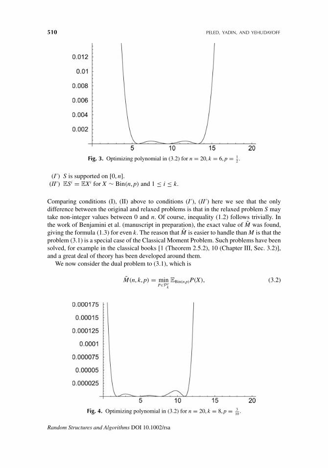
Fig. 3. Optimizing polynomial in (3.2) for n = 20, k = 6, p = 12 .
(I ′) S is supported on [0, n].(II ′) ESi = EXi for X ∼ Bin(n, p) and 1 ≤ i ≤ k.
Comparing conditions (I), (II) above to conditions (I ′), (II ′) here we see that the onlydifference between the original and relaxed problems is that in the relaxed problem S maytake non-integer values between 0 and n. Of course, inequality (1.2) follows trivially. Inthe work of Benjamini et al. (manuscript in preparation), the exact value of M was found,giving the formula (1.3) for even k. The reason that M is easier to handle than M is that theproblem (3.1) is a special case of the Classical Moment Problem. Such problems have beensolved, for example in the classical books [1 (Theorem 2.5.2), 10 (Chapter III, Sec. 3.2)],and a great deal of theory has been developed around them.
We now consider the dual problem to (3.1), which is
M(n, k, p) = minP∈Pc
k
EBin(n,p)P(X), (3.2)
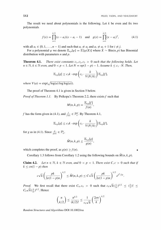
Fig. 4. Optimizing polynomial in (3.2) for n = 20, k = 8, p = 310 .
Random Structures and Algorithms DOI 10.1002/rsa

MAXIMAL PROBABILITY FOR 1 511
where Pck is the collection of polynomials P : R → R of degree at most k satisfying P(x) ≥ 0
for x ∈ [0, n) and P(n) ≥ 1 (the c stands for continuous). The optimizing polynomial isexplicitly given in [1], it equals 1 at n and for even k it has k
2 double roots in [0, n) (for odd kit has one root at 0 and k−1
2 double roots in (0, n)). The location of the roots is given in termsof Krawtchouk polynomials, the orthogonal polynomials of the Binomial distribution. InFigures 3 and 4 we have drawn the optimizing polynomials for some specific parameters.More details on the optimizing polynomials are given by Benjamini et al. (manuscript inpreparation).
It seems worth mentioning that for even k there is another problem which is equivalent tothe relaxed dual problem (3.2). This other problem has been used by some authors to obtainsimilar upper bounds, sometimes without noting the equivalence to (3.2). This equivalence isalso fundamental in the analysis of the Classical Moment Problem. The equivalent problemfor even k is
M(n, k, p) = minP∈P2
k
EBin(n,p)P(X), (3.3)
where P2k is the collection of polynomials P : R → R of the form P = R2 where R is
a polynomial of degree at most k2 satisfying |R(n)| ≥ 1. It is clear that P2
k ⊆ Pck but in
fact they are equal. This follows immediately from the Markov-Lukacs theorem (see forexample [10, Chapter III, Theorem 2.2]).
Theorem 3.1 (Markov-Lukacs). A polynomial P of even degree is non-negative on [a, b]iff it is of the form
P(x) = R2(x) + (x − a)(b − x)Q2(x) (3.4)
for some polynomials Q and R.
4. PROOF OF MAIN RESULT
In this section we show how to reduce our main result, Theorem 1.1, to a result aboutpolynomials. We also give the estimate on M(n, k, p) required to deduce Corollary 1.3 fromCorollary 1.2.
Theorem 1.1 is proved using the following general idea. Consider any polynomial P ∈ Pdk
of the form given in Prékopa’s Theorem 2.2. Change the location of its roots slightly tomake each pair of adjacent roots into one double root. The new perturbed polynomial P isin Pc
k . Show that the expectation under the Bin(n, p) distribution of P is not much higherthan that of P. Deduce that the expectation of the optimal polynomial in (2.5) is not muchlower than the expectation of the optimal polynomial in (3.2).
The actual proof that the two expectations are close is somewhat complicated. A keyingredient is the use of discrete Chebyshev polynomials to bound the ratio of the value of Pand P at certain points. The Chebyshev polynomials were previously used in a similar con-text; see, for example [9]; “Approximate inclusion-exclusion and orthogonal polynomials”,Samorodnitsky, unpublished manuscript (1999).
Random Structures and Algorithms DOI 10.1002/rsa
512 PELED, YADIN, AND YEHUDAYOFF
The result we need about polynomials is the following. Let k be even and fix twopolynomials
f (x) =k/2∏i=1
(x − ai)(x − ai − 1) and g(x) =k/2∏i=1
(x − ai)2, (4.1)
with all ai ∈ {0, 1, . . . , n − 1} and such that ai �= aj and ai �= aj + 1 for i �= j.For a polynomial ϕ we denote En,p[ϕ] = E [ϕ(X)] where X ∼ Bin(n, p) has Binomial
distribution with parameters n and p.
Theorem 4.1. There exist constants c1, c2, c3 > 0 such that the following holds. Letn ∈ N, k ∈ N even, and 0 < p < 1. Let N = np(1 − p) − 1. Assume k ≤ c1 · N. Then,
En,p[g] ≤ c3k · exp
(c2 · k
V(N/k)
)En,p[f ],
where V(a) = exp(√
log(a) log log(a)).
The proof of Theorem 4.1 is given in Section 5 below.
Proof of Theorem 1.1. By Prékopa’s Theorem 2.2, there exists f such that
M(n, k, p) = En,p[f ]f (n)
,
f has the form given in (4.1), and ff (n)
∈ Pdk . By Theorem 4.1,
En,p[g] ≤ c3k · exp
(c2 · k
V(N/k)
)En,p[f ],
for g as in (4.1). Since gg(n)
∈ Pck ,
M(n, k, p) ≤ En,p[g]g(n)
,
which completes the proof, as g(n) ≥ f (n).
Corollary 1.3 follows from Corollary 1.2 using the following bounds on M(n, k, p).
Claim 4.2. Let n ∈ N, k ∈ N even, and 0 < p < 1. There exist C, c > 0 such that ifk ≤ cn(1 − p) then
c√
k
(pk
2e(1 − p)n
)k/2
≤ M(n, k, p) ≤ C√
k
(pk
2e(1 − p)n
)k/2
ek2/2n.
Proof. We first recall that there exist C4, c4 > 0 such that c4
√k( k
2e )k/2 ≤ ( k
2 )! ≤C4
√k( k
2e )k/2. Hence
(n
k/2
)≤ nk/2
(k/2)! ≤ 1
c4
√k
(2en
k
)k/2
Random Structures and Algorithms DOI 10.1002/rsa

MAXIMAL PROBABILITY FOR 1 513
and since k ≤ cn(1 − p) (for a small enough c), we have(n
k/2
)≥ (n − k/2)k/2
(k/2)! ≥ 1
C4
√k
(2en
k
)k/2
e−k2/2n.
Hence
P
(Bin(n, 1 − p) ≤ k
2
)≥
(n
k/2
)pn−k/2(1 − p)k/2
≥ pn
C4
√k
(2e(1 − p)n
pk
)k/2
e−k2/2n.
Similarly note that since k ≤ cn(1 − p), we have
(n
i
)pn−i(1 − p)i ≤ 1
2
(n
i + 1
)pn−i−1(1 − p)i+1
for i ≤ k/2. Hence
P
(Bin(n, 1 − p) ≤ k
2
)≤ 2
(n
k/2
)pn−k/2(1 − p)k/2 ≤ 2pn
c4
√k
(2e(1 − p)n
pk
)k/2
.
The claim now follows by substituting the above estimates into (1.3).
5. PERTURBING ROOTS OF POLYNOMIALS
In this section we shall prove Theorem 4.1. For n ∈ N, we denote In = {0, 1, . . . , n}. For tworeal numbers a and b, we denote [a, b) = {t : a ≤ t < b} and [a, b] = {t : a ≤ t ≤ b}.For given n ∈ N and 0 < p < 1, we define Pn,p[x] = ( n
x
)px(1 − p)n−x for x ∈ In; i.e., the
probability of x according to Bin(n, p).We wish to bound the ratio between En,p
[g]
and En,p
[f]. We write
En,p
[g]
En,p
[f] =
∑nx=0 Pn,p[x]g(x)∑nx=0 Pn,p[x]f (x) . (5.1)
The theorem then follows from the following two lemmas:
Lemma 5.1. Let x ∈ In be such that f (x) �= 0. Then
g(x)
f (x)≤ 2
√k.
Lemma 5.2. There exist universal constants c1, c2, c3 > 0 such that the following holds.Let N = np(1 − p) − 1. Assume k ≤ c1 · N. Then, for every x ∈ In there exists w ∈ In
satisfying
Pn,p[x]g(x)
Pn,p[w]f (w)≤ c3 · exp
(c2 · k
V(N/k)
), (5.2)
where V(a) = exp(√
log(a) log log(a)).
Random Structures and Algorithms DOI 10.1002/rsa

514 PELED, YADIN, AND YEHUDAYOFF
The first lemma, whose proof is much simpler than the proof of the second lemma, isproved in Section 5.1. The second lemma addresses the case f (x) = 0 in which the firstlemma does not apply, and is proved in Section 5.2. We note that the ‘simple’ ideas presentedin the proof of the first lemma can yield a weaker version of the second lemma, with a boundof the form c3 exp(c2k) on the RHS of (5.2). While significantly weaker, such a bound stillyields the correct asymptotic behavior of M(n, k, p) for constant k.
We now show how Theorem 4.1 follows from the two lemmas.
Proof of Theorem 4.1. Let
Zeros(f ) = {y ∈ In : f (y) = 0} .
We shall denote the w that corresponds to x according to Lemma 5.2 by wx. We write(5.1) using the above two lemmas and using the fact that for all x ∈ In, Pn,p[x] ≥ 0 andf (x), g(x) ≥ 0 [due to the special structure (4.1) of the polynomials] as
En,p[g] ≤ 2√
k∑
x∈In\Zeros(f )
Pn,p[x]f (x)
+ c3 · exp
(c2 · k
V(N/k)
) ∑x∈Zeros(f )
Pn,p[wx]f (wx)
≤ (c3 + 2)k · exp
(c2 · k
V(N/k)
)En,p[f ].
5.1. Points that are not zeros of f
Proof of Lemma 5.1. Note that
g(x)
f (x)=
k/2∏i=1
ai − x
ai + 1 − x. (5.3)
Since f (x) �= 0, we can partition the ai’s into two sets:
S1 = {i : ai < x} and S2 = {i : ai > x} .
First, for each i ∈ S2
0 ≤ ai − x
ai + 1 − x≤ 1. (5.4)
In addition,
0 ≤∏i∈S1
x − ai
x − ai − 1≤
k/2∏i=1
(1 + 1
2i − 1
)≤ 2exp
(k/2∑i=2
1
2i − 1
)
≤ 2exp
(1
2log(k − 1)
)≤ 2
√k. (5.5)
The lemma follows by substituting (5.4) and (5.5) in (5.3).
Random Structures and Algorithms DOI 10.1002/rsa
MAXIMAL PROBABILITY FOR 1 515
5.2. Points that are zeros of f
In this section we prove Lemma 5.2. We first describe a family of orthogonal polynomials,the discrete Chebyshev polynomials. Then we prove Claim 5.4 that uses these polynomials.Finally we use the Claim 5.4 to prove Lemma 5.2.
5.2.1. Orthogonal Polynomials. We now give some properties of a family of orthogonalpolynomials studied by Chebyshev, sometimes called discrete Chebyshev polynomials.These properties are described and proved in [17 (Section 2.8)]. We use these orthogonalpolynomial to prove the following proposition.
Proposition 5.3. Let M ∈ N and let G be a monic polynomial of degree d for 0 ≤ d ≤ M2 ,
then
maxi∈{0,...,M−1}
|G(i)| ≥ Md
4d+1/2e−d3/M2
.
Proof. The family of polynomials {td}M−1d=0 defined below are orthogonal polynomials for
the measure µM which assigns mass one to each integer x ∈ {0, 1, . . . , M − 1}, see (5.7) forthe chosen normalization. In other words for every d, d ′ ∈ {0, . . . , M − 1} such that d �= d ′,
M−1∑i=0
td(i)td′(i) = 0.
The polynomial td is
td(x) = d! · �(d)( x
d
) (x − M
d
), (5.6)
where
�G(x)def= G(x + 1) − G(x), �(d)G
def= �[�(d−1)G
]and
( x
d
)def= x(x − 1) · · · (x − d + 1)
d! .
The normalization is chosen so that
M−1∑i=0
|td(i)|2 = M(M2 − 12)(M2 − 22) · · · (M2 − d2)
2d + 1. (5.7)
The coefficient of x2d in d! · ( xd
) ( x−Md
)is 1
d! . Thus, by the linearity of �, and since for everyk ∈ N,
�xk = (x + 1)k − xk = kxk−1 +(
k
2
)xk−2 + · · · + 1,
Random Structures and Algorithms DOI 10.1002/rsa
516 PELED, YADIN, AND YEHUDAYOFF
the polynomial td has degree d, and the coefficient of xd in td is( 2d
d
). Thus, since every monic
polynomial G of degree d < M can be expanded as G(x) = ( 2dd
)−1td(x) + ∑d−1
i=0 aiti(x),we have using (5.7)
M−1∑i=0
|G(i)|2 ≥(
2d
d
)−2 M−1∑i=0
|td(i)|2
=(
2d
d
)−2 M(M2 − 12)(M2 − 22) · · · (M2 − d2)
2d + 1. (5.8)
Using the inequalities 1 − x ≥ e−2x (0 ≤ x ≤ 14 ),
( 2dd
) ≤ 2 4d√πd
(d ≥ 1), and∑d
i=1 i2 =d(d+1)(2d+1)
6 ≤ d3 (d ≥ 1) we obtain for 1 ≤ d ≤ M2 ,
M−1∑i=0
|G(i)|2 ≥ πdM2d+1
42d+1(2d + 1)e−2
∑di=1 i2/M2 ≥
(M
4
)2d+1
e−2d3/M2. (5.9)
The proposition thus follows (the case d = 0 is straightforward).
5.2.2. A Segment With Few Zeros. In this section we prove an auxiliary claim, to beused in the next section as a main component in the proof of Lemma 5.2. The claim roughlystates that given a segment with few zeros, we can find a point at which f obtains a “large”value.
Claim 5.4. Let x ∈ In, let R, m ∈ N be such that m ≥ 2R, let L be a non-negative integer,and let τ > 4. If
|Zeros(f ) ∩ [x + m, x + τm)| ≤ R, (5.10)
and
|Zeros(f ) ∩ (x, x + m/τ)| ≥ L, (5.11)
then there exists w ∈ N ∩ [x + 2m, x + 3m] such that
g(x)
f (w)≤ 8 · exp
(12k
τ+ 6R − L log τ
).
Similarly, if instead of (5.10) and (5.11) we have
|Zeros(f ) ∩ (x − τm, x − m]| ≤ R,
and
|Zeros(f ) ∩ (x − m/τ , x)| ≥ L,
then there exists w ∈ N ∩ [x − 3m, x − 2m] such that
g(x)
f (w)≤ 8 · exp
(12k
τ+ 6R − L log τ
).
Random Structures and Algorithms DOI 10.1002/rsa
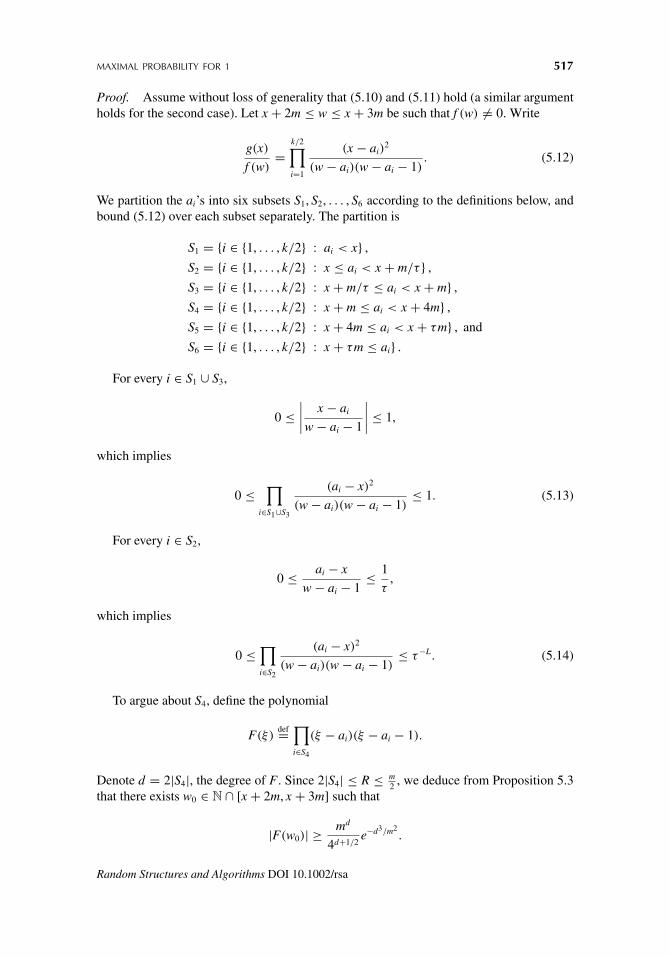
MAXIMAL PROBABILITY FOR 1 517
Proof. Assume without loss of generality that (5.10) and (5.11) hold (a similar argumentholds for the second case). Let x + 2m ≤ w ≤ x + 3m be such that f (w) �= 0. Write
g(x)
f (w)=
k/2∏i=1
(x − ai)2
(w − ai)(w − ai − 1). (5.12)
We partition the ai’s into six subsets S1, S2, . . . , S6 according to the definitions below, andbound (5.12) over each subset separately. The partition is
S1 = {i ∈ {1, . . . , k/2} : ai < x} ,
S2 = {i ∈ {1, . . . , k/2} : x ≤ ai < x + m/τ } ,
S3 = {i ∈ {1, . . . , k/2} : x + m/τ ≤ ai < x + m} ,
S4 = {i ∈ {1, . . . , k/2} : x + m ≤ ai < x + 4m} ,
S5 = {i ∈ {1, . . . , k/2} : x + 4m ≤ ai < x + τm} , and
S6 = {i ∈ {1, . . . , k/2} : x + τm ≤ ai} .
For every i ∈ S1 ∪ S3,
0 ≤∣∣∣∣ x − ai
w − ai − 1
∣∣∣∣ ≤ 1,
which implies
0 ≤∏
i∈S1∪S3
(ai − x)2
(w − ai)(w − ai − 1)≤ 1. (5.13)
For every i ∈ S2,
0 ≤ ai − x
w − ai − 1≤ 1
τ,
which implies
0 ≤∏i∈S2
(ai − x)2
(w − ai)(w − ai − 1)≤ τ−L. (5.14)
To argue about S4, define the polynomial
F(ξ)def=
∏i∈S4
(ξ − ai)(ξ − ai − 1).
Denote d = 2|S4|, the degree of F. Since 2|S4| ≤ R ≤ m2 , we deduce from Proposition 5.3
that there exists w0 ∈ N ∩ [x + 2m, x + 3m] such that
|F(w0)| ≥ md
4d+1/2e−d3/m2
.
Random Structures and Algorithms DOI 10.1002/rsa

518 PELED, YADIN, AND YEHUDAYOFF
Hence, since∏
i∈S4(ai − x)2 ≤ (4m)d ,
0 ≤∏i∈S4
(ai − x)2
(w0 − ai)(w0 − ai − 1)≤ 2 · e3R+R3/m2 ≤ 2 · e4R. (5.15)
For every i ∈ S5,
0 ≤ ai − x
ai − w≤ 4.
Hence, since |S5| ≤ R+12 ,
0 ≤∏i∈S5
(ai − x)2
(ai − w)(ai + 1 − w)≤ 4 · 4R. (5.16)
Similarly, since 2|S6| ≤ k,
0 ≤∏i∈S6
(ai − x)2
(ai − w)(ai + 1 − w)≤
(τ
τ − 3
)2|S6|≤ exp
(12k
τ
). (5.17)
Therefore, plugging (5.14), (5.13), (5.16), (5.17) and (5.15) into (5.12) with w = w0,
g(x)
f (w0)≤ 8 · exp
(12k
τ+ 6R − L log τ
).
5.2.3. Finding good w. The following claim shows that there exists a w that is “close”to x on which f obtains a “large” value.
Claim 5.5. Let x ∈ In, k ≥ Z ∈ N, and τ ≥ e12. Let K be the smallest integer such that
⌊log τ
6
⌋K−12 ≥ k
Z.
Then, there exist integers w1 > x and w2 < x such that for each w ∈ {w1, w2},3Z ≤ |w − x| ≤ 9ZτK
and
g(x)
f (w)≤ 8 · exp
(12k
τ+ 6Z
).
Proof. We show the existence of w1, the existence of w2 can be shown similarly.Let Z0 = Z1 = Z . Let m0 = 3Z0 and m1 = τm0. If either
|Zeros(f ) ∩ [x + m0, x + m1)| ≤ Z0 (5.18)
Random Structures and Algorithms DOI 10.1002/rsa
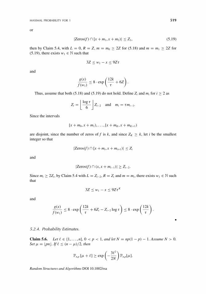
MAXIMAL PROBABILITY FOR 1 519
or
|Zeros(f ) ∩ [x + m1, x + m2)| ≤ Z1, (5.19)
then by Claim 5.4, with L = 0, R = Z , m = m0 ≥ 2Z for (5.18) and m = m1 ≥ 2Z for(5.19), there exists w1 ∈ N such that
3Z ≤ w1 − x ≤ 9Zτ
and
g(x)
f (w1)≤ 8 · exp
(12k
τ+ 6Z
).
Thus, assume that both (5.18) and (5.19) do not hold. Define Zi and mi for i ≥ 2 as
Zi =⌊
log τ
6
⌋Zi−2 and mi = τmi−1.
Since the intervals
[x + m0, x + m1), . . . , [x + mK , x + mK+1)
are disjoint, since the number of zeros of f is k, and since ZK ≥ k, let i be the smallestinteger so that
|Zeros(f ) ∩ [x + mi, x + mi+1)| ≤ Zi
and
|Zeros(f ) ∩ (x, x + mi−1)| ≥ Zi−2.
Since mi ≥ 2Zi, by Claim 5.4 with L = Zi−2, R = Zi and m = mi, there exists w1 ∈ N suchthat
3Z ≤ w1 − x ≤ 9ZτK
and
g(x)
f (w1)≤ 8 · exp
(12k
τ+ 6Zi − Zi−2 log τ
)≤ 8 · exp
(12k
τ
).
5.2.4. Probability Estimates.
Claim 5.6. Let ∈ {1, . . . , n}, 0 < p < 1, and let N = np(1 − p) − 1. Assume N > 0.Set µ = pn. If ≤ (n − µ)/2, then
Pn,p [µ + ] ≥ exp
(−32
2N
)Pn,p[µ].
Random Structures and Algorithms DOI 10.1002/rsa

520 PELED, YADIN, AND YEHUDAYOFF
In addition, if ≤ µ/2, then
Pn,p [µ − ] ≥ exp
(−82
N
)Pn,p[µ].
Proof. Assume that − 1 ≤ (n − µ)/2. Then,
Pn,p[µ]Pn,p[µ + ] =
(1 − p
p
)
· µ∏
i=1(1 + i/µ)
(n − µ)∏−1
i=0 (1 − i/(n − µ))
≤(
1 − p
p
)
· µ
(n − µ)exp
(∑
i=1
i
µ+ 2(i − 1)
n − µ
)
=(
1 − p
p
)
· µ
(n − µ)exp
( ·
(( + 1)(n − µ) + 2µ( − 1)
2µ(n − µ)
))
≤ exp
( ·
((n + µ) + n
2µ(n − µ)
))
≤ exp
(32
2n·(
1
p(1 − p) − 1/n
)).
This proves the first assertion. For the second assertion note that
≤ µ
2≤ �pn
2= n − (1 − p)n
2.
Recall that the binomial measure decreases as the distance from its expectation increases.Thus,
Pn,p[µ − ] = Pn,(1−p)[n − µ + ] ≥ Pn,(1−p)[(1 − p)n + 1 + ].
In addition, since ( + 1) − 1 ≤ n−(1−p)n2 , the proof of the first assertion implies
Pn,p[µ] ≤ exp
(3
2N
)· Pn,p[µ + 1]
≤ exp
(3
2N
)· Pn,p[n − (1 − p)n]
= exp
(3
2N
)· Pn,(1−p)[(1 − p)n]
≤ exp
(3
2N
)· exp
(3( + 1)2
2N
)· Pn,(1−p)
[(1 − p)n + 1 + ]
≤ exp
(3(( + 1)2 + 1)
2N
)· Pn,p[µ − ],
which completes the proof since ≥ 1.
Random Structures and Algorithms DOI 10.1002/rsa
MAXIMAL PROBABILITY FOR 1 521
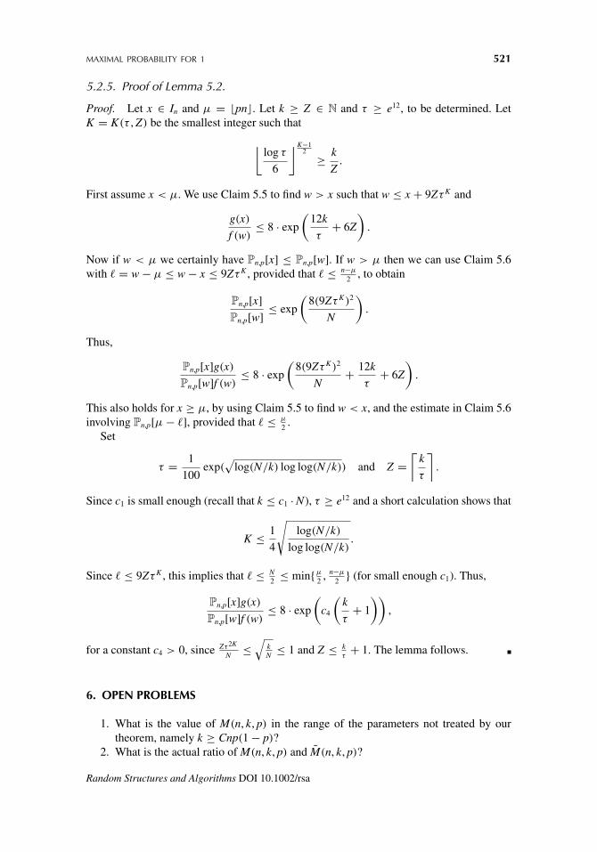
5.2.5. Proof of Lemma 5.2.
Proof. Let x ∈ In and µ = pn. Let k ≥ Z ∈ N and τ ≥ e12, to be determined. LetK = K(τ , Z) be the smallest integer such that
⌊log τ
6
⌋K−12 ≥ k
Z.
First assume x < µ. We use Claim 5.5 to find w > x such that w ≤ x + 9ZτK and
g(x)
f (w)≤ 8 · exp
(12k
τ+ 6Z
).
Now if w < µ we certainly have Pn,p[x] ≤ Pn,p[w]. If w > µ then we can use Claim 5.6with = w − µ ≤ w − x ≤ 9ZτK , provided that ≤ n−µ
2 , to obtain
Pn,p[x]Pn,p[w] ≤ exp
(8(9ZτK)2
N
).
Thus,
Pn,p[x]g(x)
Pn,p[w]f (w)≤ 8 · exp
(8(9ZτK)2
N+ 12k
τ+ 6Z
).
This also holds for x ≥ µ, by using Claim 5.5 to find w < x, and the estimate in Claim 5.6involving Pn,p[µ − ], provided that ≤ µ
2 .Set
τ = 1
100exp(
√log(N/k) log log(N/k)) and Z =
⌈k
τ
⌉.
Since c1 is small enough (recall that k ≤ c1 · N), τ ≥ e12 and a short calculation shows that
K ≤ 1
4
√log(N/k)
log log(N/k).
Since ≤ 9ZτK , this implies that ≤ N2 ≤ min{µ
2 , n−µ
2 } (for small enough c1). Thus,
Pn,p[x]g(x)
Pn,p[w]f (w)≤ 8 · exp
(c4
(k
τ+ 1
)),
for a constant c4 > 0, since Zτ2K
N ≤√
kN ≤ 1 and Z ≤ k
τ+ 1. The lemma follows.
6. OPEN PROBLEMS
1. What is the value of M(n, k, p) in the range of the parameters not treated by ourtheorem, namely k ≥ Cnp(1 − p)?
2. What is the actual ratio of M(n, k, p) and M(n, k, p)?
Random Structures and Algorithms DOI 10.1002/rsa

522 PELED, YADIN, AND YEHUDAYOFF
3. Is there also a similarity between the optimal distributions of our original and relaxedproblems [problems (2.3) and (3.1)]? As explained in Section 2, this is related towhether the optimizing polynomials in the dual problems are similar. As hinted byFigures 1–4, calculations in particular cases seem to indicate this to be the case. Thesimilarity seems especially strong in the case p = 1
2 .4. In the setting of Theorem 4.1, what is the best ratio between En,p[g] and En,p[f ]?
i.e., the best bound on the change in the expectation of the polynomial after smallperturbation of its zeros.
5. Find upper and lower bounds for the maximal probability that all the bits are 1, forthe class of almost k-wise independent distributions. Similarly to k-wise independentdistributions, such distributions have also proven quite useful for the derandomizationof algorithms in computer science.
ACKNOWLEDGMENTS
The authors thank Itai Benjamini, Ori Gurel-Gurevich, and Simon Litsyn for several usefuldiscussions on this problem. Part of this work was conducted while the authors participatedin the PCMI Graduate Summer School at Park City, Utah, July 2007.
APPENDIX
We provide here short proofs for the results of Benjamini et al. (manuscript in preparation)that we use.
Proof of (1.1). Fix n ∈ N, 0 < p < 1, and an odd k ∈ N. Let P be the optimal polynomialfor the problem (2.5) for these n, k, and p. By the second part of Theorem (2.2) we knowthat
P(z) = z∏(k−1)/2
i=1 (z − z2i)(z − z2i+1)
n∏(k−1)/2
i=1 (n − z2i)(n − z2i+1). (A1)
Now note that
EBin(n,p)P(Z)
=n∑
z=0
z∏(k−1)/2
i=1 (z − z2i)(z − z2i+1)
n∏(k−1)/2
i=1 (n − z2i)(n − z2i+1)
(n
z
)pz(1 − p)n−z
=n∑
z=1
∏(k−1)/2i=1 (z − z2i)(z − z2i+1)∏(k−1)/2i=1 (n − z2i)(n − z2i+1)
(n − 1
z − 1
)pz(1 − p)n−z
= pn−1∑z=0
∏(k−1)/2i=1 (z − (z2i − 1))(z − (z2i+1 − 1))∏(k−1)/2
i=1 (n − z2i)(n − z2i+1)
(n − 1
z
)pz(1 − p)n−1−z
= p · EBin(n−1,p)Q(Z),
(A2)
where
Q(z) =∏(k−1)/2
i=1 (z − (z2i − 1))(z − (z2i+1 − 1))∏(k−1)/2i=1 (n − 1 − (z2i − 1))(n − 1 − (z2i+1 − 1))
. (A3)
Random Structures and Algorithms DOI 10.1002/rsa
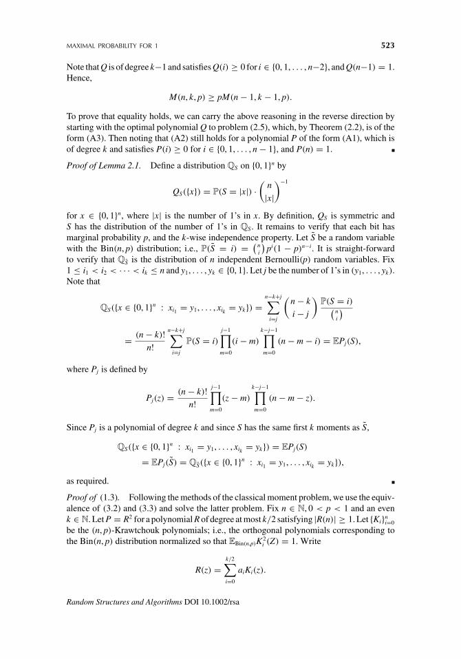
MAXIMAL PROBABILITY FOR 1 523
Note that Q is of degree k−1 and satisfies Q(i) ≥ 0 for i ∈ {0, 1, . . . , n−2}, and Q(n−1) = 1.Hence,
M(n, k, p) ≥ pM(n − 1, k − 1, p).
To prove that equality holds, we can carry the above reasoning in the reverse direction bystarting with the optimal polynomial Q to problem (2.5), which, by Theorem (2.2), is of theform (A3). Then noting that (A2) still holds for a polynomial P of the form (A1), which isof degree k and satisfies P(i) ≥ 0 for i ∈ {0, 1, . . . , n − 1}, and P(n) = 1.
Proof of Lemma 2.1. Define a distribution QS on {0, 1}n by
QS({x}) = P(S = |x|) ·(
n
|x|)−1
for x ∈ {0, 1}n, where |x| is the number of 1’s in x. By definition, QS is symmetric andS has the distribution of the number of 1’s in QS. It remains to verify that each bit hasmarginal probability p, and the k-wise independence property. Let S be a random variablewith the Bin(n, p) distribution; i.e., P(S = i) = ( n
i
)pi(1 − p)n−i. It is straight-forward
to verify that QS is the distribution of n independent Bernoulli(p) random variables. Fix1 ≤ i1 < i2 < · · · < ik ≤ n and y1, . . . , yk ∈ {0, 1}. Let j be the number of 1’s in (y1, . . . , yk).Note that
QS({x ∈ {0, 1}n : xi1 = y1, . . . , xik = yk}) =n−k+j∑
i=j
(n − k
i − j
)P(S = i)( n
i
)= (n − k)!
n!n−k+j∑
i=j
P(S = i)j−1∏m=0
(i − m)
k−j−1∏m=0
(n − m − i) = EPj(S),
where Pj is defined by
Pj(z) = (n − k)!n!
j−1∏m=0
(z − m)
k−j−1∏m=0
(n − m − z).
Since Pj is a polynomial of degree k and since S has the same first k moments as S,
QS({x ∈ {0, 1}n : xi1 = y1, . . . , xik = yk}) = EPj(S)
= EPj(S) = QS({x ∈ {0, 1}n : xi1 = y1, . . . , xik = yk}),as required.
Proof of (1.3). Following the methods of the classical moment problem, we use the equiv-alence of (3.2) and (3.3) and solve the latter problem. Fix n ∈ N, 0 < p < 1 and an evenk ∈ N. Let P = R2 for a polynomial R of degree at most k/2 satisfying |R(n)| ≥ 1. Let {Ki}n
i=0
be the (n, p)-Krawtchouk polynomials; i.e., the orthogonal polynomials corresponding tothe Bin(n, p) distribution normalized so that EBin(n,p)K2
i (Z) = 1. Write
R(z) =k/2∑i=0
aiKi(z).
Random Structures and Algorithms DOI 10.1002/rsa
524 PELED, YADIN, AND YEHUDAYOFF
Note that
EBin(n,p)P(Z) = EBin(n,p)R2(Z) =
k/2∑i=0
a2i .
Hence the problem (3.3) reduces to minimizing∑k/2
i=0 a2i under the constraint that |R(n)| =
| ∑k/2i=0 aiKi(n)| ≥ 1. By Cauchy-Schwarz,
k/2∑i=0
a2i
k/2∑i=0
K2i (n) ≥
(k/2∑i=0
aiKi(n)
)2
≥ 1.
Hence the optimal value of the problem (3.3) is 1∑k/2i=0 K2
i (n)and the optimal polynomial is
[up to multiplication by (−1)]
R(z) = 1∑k/2i=0 K2
i (n)
k/2∑i=0
Ki(n)Ki(z).
Since the Krawtchouk polynomials equal [17]
Ki(x) =(n
i
)− 12(p(1 − p))− i
2
i∑j=0
(−1)i−j
(n − x
i − j
) (x
j
)pi−j(1 − p)j,
and in particular
Ki(n) =(n
i
) 12(
1 − p
p
) i2
,
we deduce (1.3).
REFERENCES
[1] N. I. Akhiezer, The classical moment problem and some related questions in analysis,Translated by N. Kemmer, Hafner Publishing, New York, 1965.
[2] N. Alon and J. Spencer, The probabilistic method, 2nd edition, Wiley, New York, 2000.
[3] C. E. Bonferroni, Teoria Statistica delle Classi e Calcolo delle probabilità, Volume in onore diRicardo Dalla Volta, Università di Firenze, 1937, pp. 1–62.
[4] G. Boole, An investigation of the laws of thought on which are founded the mathematicaltheories of logic and probabilities, Dover, New York, 1854.
[5] E. Boros and A. Prékopa, Closed form two-sided bounds for probabilities that at least r andexactly r out of n events occur, Math Oper Res 14 (1989), 317–342.
[6] D. A. Dawson and D. Sankoff, An inequality for probabilities, Proc Am Math Soc 18 (1967),504–507.
[7] I. Dumer and S. Yekhanin, Long nonbinary codes exceeding the Gilbert-Varshamov bound forany fixed distance, IEEE Trans Inform Theory 50 (2004), 2357–2362.
[8] J. Galambos and T. Xu, A new method of generating Bonferroni-type inequalities by iteration,Math Proc Cambridge Philos Soc 107 (1990), 601–607.
Random Structures and Algorithms DOI 10.1002/rsa
MAXIMAL PROBABILITY FOR 1 525
[9] I. S. Honkala, T. Laihonen, and S. Litsyn, On covering radius and discrete Chebyshevpolynomials, Appl Algebra Eng, Commun Comput 8 (1997), 395–401.
[10] M. G. Kreın and A. A. Nudel’man, The Markov moment problem and extremal problems, Ideasand problems of P. L. Cebyšev and A. A. Markov and their further development, Translatedfrom the Russian by D. Louvish, Translations of mathematical monographs, Vol. 50, AmericanMathematical Society, Providence, RI, 1977.
[11] S. M. Kwerel, Most stringent bounds on aggregated probabilities of partially specifieddependent probability systems, J Am Stat Assoc 70 (1975), 472–479.
[12] N. Linial and N. Nisan, Approximate inclusion-exclusion, Combinatorica 10 (1990), 349–365.
[13] M. Luby and A. Wigderson, Pairwise independence and derandomization, Technical ReportTR-95-035, International Computer Science Institute, Berkeley, California, 1995.
[14] F. J. MacWilliams and N. J. A. Sloane, The theory of error-correcting codes, North-HollandMathematical Library, Vol. 16, North-Holland, Amsterdam, 1977.
[15] R. Meshulam, On subsets of finite abelian groups containing no 3-term arithmetic progressions,J Comb Theory Ser A 71 (1995), 168–172.
[16] A. Prékopa, Boole-Bonferroni inequalities and linear programming, Oper Res 36 (1988),145–162.
[17] G. Szego, Orthogonal polynomials, 4th edition, Vol. XXIII, American Mathematical Society,Colloquium Publications, Providence, RI, 1975.
Random Structures and Algorithms DOI 10.1002/rsa
![Maximal Forklift [Master Brochure]](https://static.fdocuments.in/doc/165x107/5571f82349795991698cb8bf/maximal-forklift-master-brochure.jpg)


![Improved Algorithms for Maximal Clique Search in Uncertain ... Algorithms for Maximal... · maximal clique model which has also been extensively studied in the literature [7], [8],](https://static.fdocuments.in/doc/165x107/5d4f555588c9937a2b8b9969/improved-algorithms-for-maximal-clique-search-in-uncertain-algorithms-for-maximal.jpg)