The Mathematics of Nonlinear Opticscachescan.bcub.ro/2008_05_28/E-book/580770-169-313.pdf · The...
145
CHAPTER 3 The Mathematics of Nonlinear Optics Guy M´ etivier Universit´ e Bordeaux 1, IMB UMR 5251, 351 Cours de la Lib´ eration, 33405 Talence Cedex, France E-mail: [email protected] Contents 1. Introduction ................................................. 173 2. Examples of equations arising in nonlinear optics ............................. 177 3. The framework of hyperbolic systems ................................... 183 3.1. Equations ............................................... 183 3.2. The dispersion relation & polarization conditions .......................... 185 3.3. Existence and stability ........................................ 188 3.4. Continuation of solutions ....................................... 190 3.5. Global existence ............................................ 191 3.6. Local results .............................................. 193 4. Equations with parameters ......................................... 195 4.1. Singular equations ........................................... 195 4.1.1. The weakly nonlinear case .................................. 196 4.1.2. The case of prepared data ................................... 197 4.1.3. Remarks on the commutation method ............................ 200 4.1.4. Application 1 ......................................... 202 4.1.5. Application 2 ......................................... 203 4.2. Equations with rapidly varying coefficients .............................. 207 5. Geometrical Optics ............................................. 209 5.1. Linear geometric optics ........................................ 210 5.1.1. An example using Fourier synthesis ............................. 210 5.1.2. The BKW method and formal solutions ........................... 211 5.1.3. The dispersion relation and phases .............................. 212 5.1.4. The propagator of amplitudes ................................. 213 5.1.5. Construction of WKB solutions ................................ 219 5.1.6. Approximate solutions .................................... 221 5.1.7. Exact solutions ........................................ 222 HANDBOOK OF DIFFERENTIAL EQUATIONS Evolutionary Equations, Volume 5 Edited by C.M. Dafermos and M. Pokorn ´ y c 2009 Elsevier B.V. All rights reserved DOI: 10.1016/S1874-5717(08)00210-7 169
Transcript of The Mathematics of Nonlinear Opticscachescan.bcub.ro/2008_05_28/E-book/580770-169-313.pdf · The...

CHAPTER 3
The Mathematics of Nonlinear Optics
Guy MetivierUniversite Bordeaux 1, IMB UMR 5251, 351 Cours de la Liberation, 33405 Talence Cedex, France
E-mail: [email protected]
Contents1. Introduction . . . . . . . . . . . . . . . . . . . . . . . . . . . . . . . . . . . . . . . . . . . . . . . . . 1732. Examples of equations arising in nonlinear optics . . . . . . . . . . . . . . . . . . . . . . . . . . . . . 1773. The framework of hyperbolic systems . . . . . . . . . . . . . . . . . . . . . . . . . . . . . . . . . . . 183
3.1. Equations . . . . . . . . . . . . . . . . . . . . . . . . . . . . . . . . . . . . . . . . . . . . . . . 1833.2. The dispersion relation & polarization conditions . . . . . . . . . . . . . . . . . . . . . . . . . . 1853.3. Existence and stability . . . . . . . . . . . . . . . . . . . . . . . . . . . . . . . . . . . . . . . . 1883.4. Continuation of solutions . . . . . . . . . . . . . . . . . . . . . . . . . . . . . . . . . . . . . . . 1903.5. Global existence . . . . . . . . . . . . . . . . . . . . . . . . . . . . . . . . . . . . . . . . . . . . 1913.6. Local results . . . . . . . . . . . . . . . . . . . . . . . . . . . . . . . . . . . . . . . . . . . . . . 193
4. Equations with parameters . . . . . . . . . . . . . . . . . . . . . . . . . . . . . . . . . . . . . . . . . 1954.1. Singular equations . . . . . . . . . . . . . . . . . . . . . . . . . . . . . . . . . . . . . . . . . . . 195
4.1.1. The weakly nonlinear case . . . . . . . . . . . . . . . . . . . . . . . . . . . . . . . . . . 1964.1.2. The case of prepared data . . . . . . . . . . . . . . . . . . . . . . . . . . . . . . . . . . . 1974.1.3. Remarks on the commutation method . . . . . . . . . . . . . . . . . . . . . . . . . . . . 2004.1.4. Application 1 . . . . . . . . . . . . . . . . . . . . . . . . . . . . . . . . . . . . . . . . . 2024.1.5. Application 2 . . . . . . . . . . . . . . . . . . . . . . . . . . . . . . . . . . . . . . . . . 203
4.2. Equations with rapidly varying coefficients . . . . . . . . . . . . . . . . . . . . . . . . . . . . . . 2075. Geometrical Optics . . . . . . . . . . . . . . . . . . . . . . . . . . . . . . . . . . . . . . . . . . . . . 209
5.1. Linear geometric optics . . . . . . . . . . . . . . . . . . . . . . . . . . . . . . . . . . . . . . . . 2105.1.1. An example using Fourier synthesis . . . . . . . . . . . . . . . . . . . . . . . . . . . . . 2105.1.2. The BKW method and formal solutions . . . . . . . . . . . . . . . . . . . . . . . . . . . 2115.1.3. The dispersion relation and phases . . . . . . . . . . . . . . . . . . . . . . . . . . . . . . 2125.1.4. The propagator of amplitudes . . . . . . . . . . . . . . . . . . . . . . . . . . . . . . . . . 2135.1.5. Construction of WKB solutions . . . . . . . . . . . . . . . . . . . . . . . . . . . . . . . . 2195.1.6. Approximate solutions . . . . . . . . . . . . . . . . . . . . . . . . . . . . . . . . . . . . 2215.1.7. Exact solutions . . . . . . . . . . . . . . . . . . . . . . . . . . . . . . . . . . . . . . . . 222
HANDBOOK OF DIFFERENTIAL EQUATIONSEvolutionary Equations, Volume 5Edited by C.M. Dafermos and M. Pokornyc© 2009 Elsevier B.V. All rights reserved
DOI: 10.1016/S1874-5717(08)00210-7
169

170 G. Metivier
5.2. Weakly nonlinear geometric optics . . . . . . . . . . . . . . . . . . . . . . . . . . . . . . . . . . 2235.2.1. Asymptotic equations . . . . . . . . . . . . . . . . . . . . . . . . . . . . . . . . . . . . . 2245.2.2. The structure of the profile equations I: the dispersive case . . . . . . . . . . . . . . . . . 2265.2.3. The structure of the profile equation II: the non-dispersive case; the generic Burger’s equation2285.2.4. Approximate and exact solutions . . . . . . . . . . . . . . . . . . . . . . . . . . . . . . . 230
5.3. Strongly nonlinear expansions . . . . . . . . . . . . . . . . . . . . . . . . . . . . . . . . . . . . 2325.3.1. An example: two levels Maxwell–Bloch equations . . . . . . . . . . . . . . . . . . . . . . 2335.3.2. A class of semi-linear systems . . . . . . . . . . . . . . . . . . . . . . . . . . . . . . . . 2345.3.3. Field equations and relativity . . . . . . . . . . . . . . . . . . . . . . . . . . . . . . . . . 2365.3.4. Linearly degenerate oscillations . . . . . . . . . . . . . . . . . . . . . . . . . . . . . . . 2365.3.5. Fully nonlinear geometric optics . . . . . . . . . . . . . . . . . . . . . . . . . . . . . . . 240
5.4. Caustics . . . . . . . . . . . . . . . . . . . . . . . . . . . . . . . . . . . . . . . . . . . . . . . . 2445.4.1. Example: spherical waves . . . . . . . . . . . . . . . . . . . . . . . . . . . . . . . . . . . 2445.4.2. Focusing before caustics . . . . . . . . . . . . . . . . . . . . . . . . . . . . . . . . . . . 2475.4.3. Oscillations past caustics . . . . . . . . . . . . . . . . . . . . . . . . . . . . . . . . . . . 247
6. Diffractive optics . . . . . . . . . . . . . . . . . . . . . . . . . . . . . . . . . . . . . . . . . . . . . . 2516.1. The origin of the Schrodinger equation . . . . . . . . . . . . . . . . . . . . . . . . . . . . . . . . 251
6.1.1. A linear example . . . . . . . . . . . . . . . . . . . . . . . . . . . . . . . . . . . . . . . 2516.1.2. Formulating the Ansatz . . . . . . . . . . . . . . . . . . . . . . . . . . . . . . . . . . . . 2526.1.3. First equations for the profiles . . . . . . . . . . . . . . . . . . . . . . . . . . . . . . . . 2546.1.4. The operator S as a Schrodinger operator . . . . . . . . . . . . . . . . . . . . . . . . . . 255
6.2. Construction of solutions . . . . . . . . . . . . . . . . . . . . . . . . . . . . . . . . . . . . . . . 2576.2.1. The non-dispersive case with odd nonlinearities and odd profiles . . . . . . . . . . . . . . 2576.2.2. Dispersive equations; the Schrodinger equation as a generic model for diffractive optics . . 2616.2.3. Rectification . . . . . . . . . . . . . . . . . . . . . . . . . . . . . . . . . . . . . . . . . . 262
6.3. Other diffractive regimes . . . . . . . . . . . . . . . . . . . . . . . . . . . . . . . . . . . . . . . 2657. Wave interaction and multi-phase expansions . . . . . . . . . . . . . . . . . . . . . . . . . . . . . . . 266
7.1. Examples of phase generation . . . . . . . . . . . . . . . . . . . . . . . . . . . . . . . . . . . . 2667.1.1. Generation of harmonics . . . . . . . . . . . . . . . . . . . . . . . . . . . . . . . . . . . 2667.1.2. Resonance and phase matching; weak vs. strong coherence . . . . . . . . . . . . . . . . . 2677.1.3. Strong coherence and small divisors . . . . . . . . . . . . . . . . . . . . . . . . . . . . . 2687.1.4. Periodic initial data may lead to almost periodic solutions . . . . . . . . . . . . . . . . . . 2697.1.5. A single initial phase can generate a space of phases of infinite dimension over R . . . . . 2697.1.6. Multidimensional effects . . . . . . . . . . . . . . . . . . . . . . . . . . . . . . . . . . . 270
7.2. Description of oscillations . . . . . . . . . . . . . . . . . . . . . . . . . . . . . . . . . . . . . . 2717.2.1. Group of phases, group of frequencies . . . . . . . . . . . . . . . . . . . . . . . . . . . . 2717.2.2. The fast variables . . . . . . . . . . . . . . . . . . . . . . . . . . . . . . . . . . . . . . . 2727.2.3. Profiles and oscillations . . . . . . . . . . . . . . . . . . . . . . . . . . . . . . . . . . . . 2727.2.4. Profiles in L p and associated oscillating families . . . . . . . . . . . . . . . . . . . . . . 2737.2.5. Multi-scale weak convergence, weak profiles . . . . . . . . . . . . . . . . . . . . . . . . 274
7.3. Formal multi-phases expansions . . . . . . . . . . . . . . . . . . . . . . . . . . . . . . . . . . . 2747.3.1. Phases and profiles. Weak coherence . . . . . . . . . . . . . . . . . . . . . . . . . . . . . 2747.3.2. Phases and profiles for the Cauchy problem . . . . . . . . . . . . . . . . . . . . . . . . . 2767.3.3. Formal BKW expansions . . . . . . . . . . . . . . . . . . . . . . . . . . . . . . . . . . . 2777.3.4. Determination of the main profiles . . . . . . . . . . . . . . . . . . . . . . . . . . . . . . 2797.3.5. Main profiles for the Cauchy problem . . . . . . . . . . . . . . . . . . . . . . . . . . . . 2807.3.6. Approximate solutions at order o(1) in L2 . . . . . . . . . . . . . . . . . . . . . . . . . . 2837.3.7. Strong coherence . . . . . . . . . . . . . . . . . . . . . . . . . . . . . . . . . . . . . . . 2847.3.8. Higher order profiles, approximate solutions at all order . . . . . . . . . . . . . . . . . . . 285
7.4. Exact oscillating solutions . . . . . . . . . . . . . . . . . . . . . . . . . . . . . . . . . . . . . . 2867.4.1. Oscillating solutions with complete expansions . . . . . . . . . . . . . . . . . . . . . . . 2867.4.2. Prepared data, continuation of solutions . . . . . . . . . . . . . . . . . . . . . . . . . . . 2867.4.3. Construction of solutions. General oscillating data . . . . . . . . . . . . . . . . . . . . . . 2887.4.4. The case of constant coefficients and planar phases . . . . . . . . . . . . . . . . . . . . . 290
7.5. Asymptotics of exact solutions . . . . . . . . . . . . . . . . . . . . . . . . . . . . . . . . . . . . 2927.5.1. The method of simultaneous approximations . . . . . . . . . . . . . . . . . . . . . . . . . 2927.5.2. The filtering method . . . . . . . . . . . . . . . . . . . . . . . . . . . . . . . . . . . . . . 294
The mathematics of nonlinear optics 171
7.6. Further examples . . . . . . . . . . . . . . . . . . . . . . . . . . . . . . . . . . . . . . . . . . . 2977.6.1. One dimensional resonant expansions . . . . . . . . . . . . . . . . . . . . . . . . . . . . 2977.6.2. Generic phase interaction for dispersive equations . . . . . . . . . . . . . . . . . . . . . . 3017.6.3. A model for Raman interaction . . . . . . . . . . . . . . . . . . . . . . . . . . . . . . . . 3037.6.4. Maximal dissipative equations . . . . . . . . . . . . . . . . . . . . . . . . . . . . . . . . 306
References . . . . . . . . . . . . . . . . . . . . . . . . . . . . . . . . . . . . . . . . . . . . . . . . . . . 309
AbstractModeling in Nonlinear Optics, and also in other fields of Physics and Mechanics, yields
interesting and difficult problems due to the presence of several different scales of time,length, energy, etc. These notes are devoted to the introduction of mathematical tools thatcan be used in the analysis of mutliscale PDE’s. We concentrate here on oscillating wavesand hyperbolic equations. The main topic is to understand the propagation and the interactionof wave packets, using phase-amplitude descriptions. The main questions are first to find thereduced equations satisfied by the envelops of the fields, and second to rigorously justifythem. We first motivate the mathematical analysis by giving various models from optics,including Maxwell–Bloch equations and examples of Maxwell–Euler systems. Then we presenta stability analysis of solutions of nonlinear hyperbolic systems, with a particular interest in thecase of singular systems where small or large parameters are present. Next, we give the mainfeatures concerning the propagations of wave trains, both in the regime of geometric optics andin the regime of diffractive optics. We present the WKB method, the propagation along rays,the diffraction effects transversal to the beam propagations, the modulation of amplitudes. Weconstruct approximate solutions and discuss their stability, rigorously justifying, when possible,the asymptotic expansions. Finally, we discuss the most important nonlinear phenomenon of thetheory, that is the wave interaction. After a small digression devoted to general considerationsabout the mathematical modeling of multi phase oscillations, we apply these notions tointroduce important notions such as phase matching, coherence of phases and apply themin various frameworks to the construction of approximate solutions. We also present severalmethods that have been used for rigorously justifying the multi-phase expansion.
Keywords: Nonlinear optics, hyperbolic systems, stability of solutions, multiscale analysis,oscillations, wave packets, geometric optics, diffractive optics, dispersive optics, waveinteraction, phase matching, resonance, coherence of phases, profiles, Maxwell equations

The Mathematics of Nonlinear Optics 173
1. Introduction
Nonlinear optics is a very active field in physics, of primary importance and with anextremely wide range of applications. For an introduction to the physical approach, wecan refer the reader to classical text books such as [107,10,6,8,109,49,89].
Optics is about the propagation of electromagnetic waves. Nonlinear optics is moreabout the study of how high intensity light interacts with and propagates through matter.As long as the amplitude of the field is moderate, the linear theory is well adapted,and complicated fields can be described as the superposition of noninteracting simplersolutions (e.g. plane waves). Nonlinear phenomena, such as double refraction or Ramaneffect, which are examples of wave interaction, have been known for a long time, but themajor motivation for a nonlinear theory came from the discovery of the laser which madeavailable highly coherent radiations with extremely high local intensities.
Clearly, interaction is a key word in nonlinear optics. Another fundamental feature isthat many different scales are present: the wavelength, the length and the width of the beam,the duration of the pulse, the intensity of the fields, but also internal scales of the mediumsuch as the frequencies of electronic transitions etc.
Concerning the mathematical set up, the primitive models are Maxwell’s equations forthe electric and magnetic intensity fields E and H and the electric and magnetic inductionsD and B, coupled with constitutive relations between these fields and/or equations whichmodel the interaction of the fields with matter. Different models are presented in Section 2.All these equations fall into the category of nonlinear hyperbolic systems. A very importantstep in modeling is to put these equations in a dimensionless form, by a suitable choice ofunits, and deciding which phenomena, at which scale, one wants to study (see e.g. [39]).However, even in dimensionless form, the equations may contain one or several small/largeparameters. For example, one encounters singular systems of the form
A0(u)∂t u +d∑
j=1
A j (u)∂x j u + λL0u = F(u) (1.1)
with λ� 1. In addition to the parameters contained in the equation, there are other lengthscales typical to the solutions under study. In linear and nonlinear optics, one is speciallyinterested in waves packets
u(t, x) = ei(k·x−ωt)U (t, x)+ cc, (1.2)
where cc denotes the complex conjugate of the preceding term, k andω are the central wavenumber and frequency, respectively, and where the envelope U (t, x) has slow variationscompared to the rapid oscillations of the exponential:
∂j
t U � ω jU, ∂jx U � k jU. (1.3)
In dimensionless form, the wave length ε := 2πk is small (�1). An important property
is that k and ω must be linked by the dispersion relation (see Section 5). Interesting

174 G. Metivier
phenomena occur when ε ≈ λ−1. With this scaling there may be resonant interactionsbetween the electromagnetic wave and the medium, accounting for the dependence ofoptical indices on the frequency and thus for diffraction of light (see e.g. [89]).
More generally, several scales can be present in the envelope U , for instance
U = U (t, x,t√ε,
x√ε) (speckles), (1.4)
U = U (t, x, εt) (long time propagation) (1.5)
etc. The typical size of the envelope U (the intensity of the beam) is another very importantparameter.
Nonlinear systems are the appropriate framework to describe interaction of waves: wavepackets with phases ϕ j = k j · x − ω j t create, by multiplication of the exponentials, thenew phase ϕ =
∑ϕ j , which may or may not satisfy the dispersion relation. In the first
case, the oscillation with phase ϕ is propagated (or persists) as time evolves: this is thesituation of phase matching. In the second case, the oscillation is not propagated and onlycreates a lower order perturbation of the fields. These heuristic arguments are the basis ofthe formal derivation of envelope equations that can be found in physics books. It is partof the mathematical analysis to make them rigorous.
In particular, self interaction can create harmonics nϕ of a phase ϕ. Reducing this to asingle small dimensionless parameter, this leads us, for instance, to look for solutions ofthe form
u(y) = ε p U(ϕε, y), ε p U
(ϕ
ε,
y√ε, y
), ε p U
(ϕε, y, εy
)(1.6)
where y = (t, x), ϕ = (ϕ1, . . . , ϕm) and U is periodic in the first set of variables.Summing up, we see that the mathematical setup concerns high frequency and
multiscale solutions of a nonlinear hyperbolic problem. At this point we merge with manyother problems arising in physics or mechanics, in particular in fluid mechanics, where thistype of multiscale analysis is also of fundamental importance. For instance, we mentionthe problems of low Mach number flows, or fast rotating fluids, which raise very similarquestions.
These notes are intended to serve as an introduction to the field. We do not even try togive a complete overview of the existing results, that would be impossible within a singlebook, and probably useless. We will tackle only a few basic problems, with the aim ofgiving methods and landmarks in the theory. Nor do we give complete proofs, instead wewill focus on the key arguments and the main ideas.
Different models arising from optics are presented in Section 2. It is important tounderstand the variety of problems and applications which can be covered by the theory.These models will serve as examples throughout the exposition. Next, the mathematicalanalysis will present the following points:• Basic results of the theory of multi-dimensional symmetric hyperbolic systems are
recalled in in Section 3. In particular we state the classical theorem of local existence and

The Mathematics of Nonlinear Optics 175
local stability of smooth solutions1. However, this theorem is of little use when applieddirectly to the primitive equations. For high frequency solutions, it provides existence andstability in very short intervals of time, because fixed bounds for the derivatives requiresmall amplitudes. Therefore this theorem, which is basic in the theory and provides a usefulmethod, does not apply directly to high frequency and high intensity problems.
One idea to circumvent this difficulty would be to use existence theorems of solutions inenergy spaces (the minimal conditions that the physical solutions are expected to satisfy).But there is no such general existence theorem in dimension ≥2. This is why existencetheorems of energy solutions or weak solutions are important. We give examples of suchtheorems, noticing that, in these statements, the counterpart of global existence is a muchweaker stability.• In Section 4 we present two methods which can be used to build an existence and
stability theory for high frequency/high intensity solutions. The first idea is to factor outthe oscillations in the linear case or to consider directly equations for profiles U (see (1.6))in the nonlinear case, introducing the fast variables (the placeholder for ϕ/ε for instance)as independent variables. The resulting equations are singular, meaning that they havecoefficients of order ε−1. The method of Section 3 does not apply in general to suchsystems, but it can be adapted to classes of such singular equations. which satisfy symmetryand have good commutation properties.
Another idea can be used if one knows an approximate solution. It is the goal of theasymptotic methods presented below to construct such approximate solutions: they satisfythe equation up to an error term of size εm . The exact solution is sought as the approximatesolution plus a corrector, presumably of order εm or so. The equation for the correctorhas the feature that the coefficients have two components: one is not small but highlyoscillatory and known (coming from the approximate solution), the other one is not knownbut is small (it depends on the corrector). The theory of Section 3 can be adapted in thiscontext to a fairly general extent. However, there is a severe restriction, which is that theorder of approximation m must be large enough. In practice, this does not mean that mmust necessarily be very large, but it does means that knowledge of the principal term isnot sufficient.• Geometric optics is a high frequency approximation of solutions. It fits with the
corpuscular description of light, giving a particle-like description of the propagation alongrays. It concerns solutions of the form u(y) = ε p U(ϕ(y)
ε, y). The phase ϕ satisfies the
eikonal equation and the amplitude U is transported along the rays. In Section 5, wegive the elements of this description, using the WKB method (for Wentzel, Kramers andBrillouin) of asymptotic (formal) expansions. The scaling ε p for the amplitude plays animportant role in the discussion: if p is large, only linear effects are observed (at least in theleading term). There is a threshold value p0 where the nonlinear effects are launched in theequation of propagation (typically it becomes nonlinear). Its value depends on the structureof the equation and of the nonlinearity. For a general quasi-linear system, p0 = 1. This isthe standard regime of weakly nonlinear geometric optics. However, there are special caseswhere for p = 1 the transport equation remains linear; this happens when some interaction
1From the point of view of applications and physics, stability is much more significant than existence.

176 G. Metivier
coefficient vanishes. This phenomenon is called transparency and for symmetry reasons itoccurs rather frequently in applications. An example is the case of waves associated withlinearly degenerate modes. In this case it is natural to look for larger solutions with p < 1,leading to strongly nonlinear regimes. We give two examples where formal large amplitudeexpansions can be computed.
The WKB construction, when it is possible, leads to approximate solutions, uεapp. Theyare functions which satisfy the equation up to an error term that is of order εm with m large.The main question is to study the stability of such approximate solutions. In the weaklynonlinear regime, the second method evoked in the presentation above in Section 4 appliesand WKB solutions are stable, implying that the formal solutions are actually asymptoticexpansions of exact solutions. But for strongly nonlinear expansions, the answer is notsimple. Indeed, strong instabilities can occur, similar to Rayleigh instabilities in fluidmechanics. These aspects will be briefly discussed.
Another very important phenomenon is focusing and caustics. It is a linear phenomenon,which leads to concentration and amplification of amplitudes. In a nonlinear context, thelarge intensities can be over amplified, launching strongly nonlinear phenomena. Someresults of this type are presented at the end of the section. However a general analysis ofnonlinear caustics is still a wide open problem.• Diffractive optics. This is the usual regime of long time or long distance propagation.
Except for very intense and very localized phenomena, the length of propagation of a laserbeam is much larger than its width. To analyze the problem, one introduces an additionaltime scale (and possibly one can also introduce an additional scale in space). This is theslow time, typically T = εt . The propagations are governed by equations in T , so that thedescription allows for times that are O(ε−1). For such propagations, the classical linearphenomenon which is observed is diffraction of light in the direction transversal to thebeam, along long distances. The canonical model which describes this phenomenon is aSchrodinger equation, which replaces the transport equation of geometric optics. This isthe well known paraxial approximation, which also applies to nonlinear equations. Thismaterial is presented in Section 6 with the goal of clarifying the nature and the universalityof nonlinear Schrodinger equations as fundamental equations in nonlinear optics, whichare often presented as the basic equations in physics books.• Wave interaction. This is really where the nonlinear nature of the equations is rich
in applications but also of mathematical difficulties. The physical phenomenon whichis central here is the resonant interaction of waves. They can be optical waves, forinstance a pump wave interacting with scattered and back scattered waves; they can alsobe optical waves interacting with electronic transitions yielding Raman effects, etc. Animportant observation is that resonance or phase matching is a rare phenomenon : alinear combination of characteristic phases is very likely not characteristic. This does notmean that the resonance phenomenon is uninteresting, on the contrary it is of fundamentalimportance. But this suggests that, when it occurs, it should remain limited. This is moreor less correct at the level of formal or BKW expansions, if one retains only the principalterms and neglects all the alleged small residual terms. However, the mathematical analysisis much more delicate: the analysis of all the phases created by the interaction, not onlythose in the principal term, can be terribly complicated, and possibly beyond the scope ofa description by functions of finitely many variables; the focusing effects of these phases

The Mathematics of Nonlinear Optics 177
have to be taken into account; harmonic generation can cause small divisors problems... Itturns out that justification of the formal calculus requires strong assumptions, that we callcoherence. Fortunately these assumptions are realistic in applications, and thus the theoryapplies to interesting examples such as the Raman interaction evoked above. Surprisingly,the coherence assumptions are very close to, if not identical with, the commutationrequirements introduced in Section 4 for the equations with the fast variables. All theseaspects, including examples, are presented in Section 7.
There are many other important questions which are not presented in these notes. Wecan mention:
– Space propagation, transmission and boundary value problems. In the exposition, wehave adopted the point of view of describing the evolution in time, solving mainly Cauchyproblems. For physicists, the propagation is more often thought of in space: the beampropagates from one point to another, or the beam enters a medium etc. In the geometricoptics description, the two formulations are equivalent, as long as they are governed by thesame transport equations. However, for the exact equations, this is a completely differentpoint of view, with the main difficulty being that the equations are not hyperbolic in space.The correct mathematical approach is to consider transmission problems or boundary valueproblems. In this framework, new questions are reflection and transmission of waves at aboundary. Another important question is the generation of harmonics or scattered waves atboundaries. In addition, the boundary or transmission conditions may reveal instabilitieswhich may or may not be excited by the incident beam, but which in any case make themathematical analysis harder. Several references in this direction are [4,104,128,129,21,25,97,98,39].
– Short pulses. We have only considered oscillating signals, that is of the form eiωt awith a slowly varying, typically, ∂t a � ωa. For short pulses, and even more for ultrashort pulses, which do exist in physics (femtosecond lasers), the duration of the pulse (thesupport of a) is just a few periods. Therefore, the description with phase and amplitude isno longer adapted. Instead of periodic profiles, this leads us to consider confined profilesin time and space, typically in the Schwartz class. On the one hand, the problem is simplerbecause it is less nonlinear : the durations of interaction are much smaller, so the nonlineareffects require more intense fields. But on the other hand, the mathematical analysis isseriously complicated by passing from a discrete to a continuous Fourier analysis in thefast variables. Several references in this direction are [2,3,17–19,16].
2. Examples of equations arising in nonlinear optics
The propagation of an electro-magnetic field is governed by Maxwell’s equation. Thenonlinear character of the propagation has several origins: it may come from self-interaction, or from the interaction with the medium in which it propagates. The generalMaxwell’s equations (in Minkowski space-time) read (see e.g. [49,107,109]):
∂t D − curl H = − j,∂t B + curl E = 0,div B = 0,div D = q
(2.1)

178 G. Metivier
where D is the electric displacement, E the electric field vector, H the magnetic fieldvector, B the magnetic induction, j the current density and q is the charge density; c is thevelocity of light. They also imply the charge conservation law:
∂t q + div j = 0. (2.2)
We mainly consider the case where there are no free charges and no current flows ( j = 0and q = 0).
All the physics of interaction of light with matter is contained in the relations betweenthe fields. The constitutive equations read
D = εE, B = µH, (2.3)
where ε is the dielectric tensor and µ the tensor of magnetic permeability. When ε and µare known, this closes the system (2.1). Conversely, (2.3) can be seen as the definition ofε and µ and the links between the fields must be given through additional relations. In thedescription of interaction of light with matter, one uses the following constitutive relations(see [107,109]):
B = µH, D = ε0 E + P = εE (2.4)
where P is called the polarization and ε the dielectric constant. In vacuum, P = 0. Whenlight propagates in a dielectric medium, the light interacts with the atomic structure, createsdipole moments and induces the polarization P .
In the standard regimes of optics, the magnetic properties of the medium are notprominent and µ can be taken constant equal to c2
ε0with c the speed of light in vacuum
and ε0 the dielectric constant in vacuum. Below we give several models of increasingcomplexity which can be derived from (2.4), varying the relation between P and E .
• Equations in vacuum.
In a vacuum, ε = ε0 and µ = 1ε0c2 are scalar and constant. The constraint equations
div E = div B = 0 are propagated in time and the evolution is governed by the classicalwave equation
∂2t E − c21E = 0. (2.5)
• Linear instantaneous polarization.
For small or moderate values of the electric field amplitude, P depends linearly in E . Inthe simplest case when the medium is isotropic and responds instantaneously to the electricfield, P is proportional to E :
P = ε0χE (2.6)

The Mathematics of Nonlinear Optics 179
χ is the electric susceptibility. In this case, E satisfies the wave equation
n2∂2t E − c21E = 0. (2.7)
where n =√
1+ χ ≥ 1 is the refractive index of the medium. In this medium, lightpropagates at the speed c
n ≤ c.
• Crystal optics.In crystals, the isotropy is broken and D is not proportional to E . The simplest model
is obtained by taking the dielectric tensor ε in (2.3) to be a positive definite symmetricmatrix, while µ = 1
ε0c2 remains scalar. In this case the system reads:
{∂t (εE)− curl H = 0,∂t (µH)+ curl E = 0,
(2.8)
plus the constraint equations div (εE) = div B = 0, which are again propagated from theinitial conditions. That the matrix ε is not proportional to the identity reflects the anisotropyof the medium. For instance, for a bi-axial crystal ε has three distinct eigenvalues.
Moreover, in the equations above, ε is constant or depends on the space variablemodeling the homogeneity or inhomogeneity of the medium.
• Lorentz modelMatter does not respond instantaneously to stimulation by light. The delay is captured
by writing in place of (2.6)
P(x, t) = ε0
∫ t
−∞
χ(t − t ′)E(x, t ′)dt ′, (2.9)
modeling a linear relation E 7→ P , satisfying the causality principle. On the frequencyside, that is after Fourier transform in time, this relation reads
P(x, τ ) = ε0χ(τ )E(x, τ ). (2.10)
It is a simple model where the electric susceptibility χ depends on the frequency τ .In a standard model, due to Lorentz [100], of the linear dispersive behavior of
electromagnetic waves, P is given by
∂2t P + ∂t P/T1 + ω
2 P = γ E (2.11)
with positive constants ω, γ , and T1 (see also [49], chap. I-31, and II-33). Resolving thisequation yields an expression of the form (2.10). In particular
χ(τ ) =γ0
ω2 − τ 2 + iτ/T1, γ0 =
γ
ε0. (2.12)

180 G. Metivier
The physical origin of (2.11) is a model of the electron as bound to the nucleus by a Hooke’slaw spring force with characteristic frequency ω; T1 is a damping time and γ a couplingconstant.
For non-isotropic crystals, the equation reads
∂2t P + R∂t P +�P = ϒE (2.13)
where R, � and ϒ are matrices which are diagonal in the the crystal frame.
• Phenomenological modeling of nonlinear interactionIn a first attempt, nonlinear responses of the medium can be described by writing P as
a power series in E :
P(x, t) = ε0
∞∑k=1
∫χk(t − t1, . . . , t − tk)
k⊗j=1
E(x, tk)dt1 . . . dtk (2.14)
where χk is a tensor of appropriate order. The symmetry properties of the susceptibilitiesχk reflect the symmetry properties of the medium. For instance, in a centrosymmetric andisotropic crystal, the quadratic susceptibility χ2 vanishes.
The first term in the series represents the linear part and often splits P into its linear(and main) part PL and its nonlinear part PN L .
P = PL + PN L . (2.15)
Instantaneous responses correspond to susceptibilities χk which are Dirac measures att j = t . One can also mix delayed and instantaneous responses.
• Two examplesIn a centrosymmetric, homogeneous and isotropic medium (such as glass or liquid), the
first nonlinear term is cubic. A model for P with a Kerr nonlinearity is P = PL + PN Lwith
∂2t PL + ∂t PL/T1 + ω
2 PL = γ E, (2.16)
PN L = γN L |E |2 E . (2.17)
In a nonisotropic crystal (such as KDP), the nonlinearity is quadratic and modelequations for P are
∂2t PL + R∂t PL +�PL = ϒE, (2.18)
PN L = γN L(E2 E3, E1 E2, E1 E2)t . (2.19)
• The anharmonic modelTo explain nonlinear dispersive phenomena, a simple and natural model is to replace
the linear restoring force (2.11) with a nonlinear law (see [6,108])

The Mathematics of Nonlinear Optics 181
∂2t P + ∂t P/T1 + (∇V )(P) = bE . (2.20)
For small amplitude solutions, the main nonlinear effect is governed by the Taylorexpansion of V at the origin, in presence of symmetries, the first term is cubic, yielding theequation
∂2t P + ∂t P/T1 + ω
2 P − α|P|2 P = γ E . (2.21)
• Maxwell–Bloch equationsBloch’s equation are widely used in nonlinear optics textbooks as a theoretical
background for the description of the interaction between light and matter and thepropagation of laser beams in nonlinear media. They link P and the electronic state ofthe medium, which is described through a simplified quantum model, see e.g. [8,107,10,109]. The formalism of density matrices is convenient to account for statistical averagingdue, for instance, to the large number of atoms. The self-adjoint density matrix ρ satisfies
iε∂tρ = [�, ρ] − [V (E, B), ρ], (2.22)
where � is the electronic Hamiltonian in absence of an external field and V (E, B) is thepotential induced by the external electromagnetic field. For weak fields, V is expanded intoits Taylor’s series (see e.g. [109]). In the dipole approximation,
V (E, B) = E · 0, P = tr(0ρ) (2.23)
where −0 is the dipole moment operator. An important simplification is that only afinite number of eigenstates of � are retained. From the physical point of view, theyare associated with the electronic levels which are actually in interaction with theelectromagnetic field. In this case, ρ is a complex finite dimensional N×N matrix and 0 isa N × N matrix with entries in C3. It is Hermitian symmetric in the sense that 0k, j = 0 j,kso that tr(0ρ) is real. In physics books, the reduction to finite dimensional systems (2.22)comes with the introduction of phenomenological damping terms, which would force thedensity matrix to relax towards a thermodynamical equilibrium in absence of the externalfield. For simplicity, we have omitted these damping terms in the equations above. Thelarge ones only contribute to reducing the size of the effective system and the small onescontribute to perturbations which do not alter qualitatively the phenomena. Physics booksalso introduce “local field corrections” to improve the model and take into account theelectromagnetic field created by the electrons. This mainly results in changing the valuesof several constants, which is of no importance in our discussion.
The parameter ε in front of ∂t in (2.22) plays a crucial role in the model. The quantitiesω j,k/ε := (ω j −ωk)/ε, where the ω j are the eigenvalues of�, have an important physicalmeaning. They are the characteristic frequencies of the electronic transitions from the levelk to the level j and therefore related to the energies of these transitions. The interactionbetween light and matter is understood as a resonance phenomenon and the possibility ofexcitation of electrons by the field. This means that the energies of the electronic transitionsare comparable to the energy of photons. Thus, if one chooses to normalize � ≈ 1 as

182 G. Metivier
we now assume, ε is comparable to the pulsation of light. The Maxwell–Bloch modeldescribed above, is expected to be correct for weak fields and small perturbations of theground state, in particular below the ionization phenomena.
• A two levels model A simplified version of Bloch’s equations for a two levels quantumsystem for the electrons, links the polarization P of the medium and the difference Nbetween the numbers of excited and nonexcited atoms:
ε2∂t P +�2 P = γ1 N E, (2.24)
∂t N = −γ2∂t P · E . (2.25)
Here,�/ε is the frequency associated with the electronic transition between the two levels.
• Interaction Laser–PlasmaWe give here another example of systems that arise in nonlinear optics. It concerns the
propagation of light in a plasma, that is a ionized medium. A classical model for the plasmais a bifluid description for ions and electrons. Then Maxwell equations are coupled to Eulerequations for the fluids:
∂t B + c curl × E = 0, (2.26)
∂t E − c curl × B = 4πe ((n0 + ne)ve − (n0 + ni )vi ) , (2.27)
(n0 + ne) (∂tve + ve · ∇ve) = −γeTe
me∇ne
−e(n0 + ne)
me
(E +
1cve × B
), (2.28)
(n0 + ni ) (∂tvi + vi · ∇vi ) = −γi Ti
mi∇ni
+e(n0 + ni )
mi
(E +
1cvi × B
), (2.29)
∂t ne +∇ · ((n0 + ne)ve) = 0, (2.30)
∂t ni +∇ · ((n0 + ni )vi ) = 0, (2.31)
where∗ E and B are the electric and magnetic field, respectively,∗ ve and vi denote the velocities of electrons and ions, respectively,∗ n0 is the mean density of the plasma,∗ ne and ni are the variation of density with respect to the mean density n0 of electrons
and ions, respectively.Moreover,∗ c is the velocity of light in the vacuum; e is the elementary electric charge,∗ me and mi are the electron’s and ion’s masses, respectively,∗ Te and Ti are the electronic and ionic temperatures, respectively and γe and γi the
thermodynamic coefficients.For a precise description of this kind of model, we refer to classical textbooks such
as [37]. One of the main points is that the mass of the electrons is very small compared

The Mathematics of Nonlinear Optics 183
to the mass of the ions: me � mi . Since the Lorentz force is the same for the ions andthe electrons, the velocity of the ions will be negligible with respect to the velocity of theelectrons. The consequence is that one can neglect the contribution of the ions in Eq. (2.27).
3. The framework of hyperbolic systems
The equations above fall into the general framework of hyperbolic systems. In this sectionwe point out a few landmarks in this theory, concerning the local stability and existencetheory, and some results of global existence.We refer to [35,36,52,53,55,58,94,103,113]for some references to hyperbolic systems.
3.1. Equations
The general setting of quasi-linear first order systems concerns equations of the form:
A0(a, u)∂t u +d∑
j=1
A j (a, u)∂x j u = F(a, u) (3.1)
where a denotes a set of parameters, which may depend on and include the time-spacevariables (t, x) ∈ R × Rd ; the A j are N × N matrices and F is a function with valuesin RN ; they depend on the variables (a, u) varying in a subdomain of RM
× RN , and weassume that F(0, 0) = 0. (Second order equations such as (2.11) or (2.21) are reduced tofirst order by introducing Q = ∂t P .)
An important case is the case of balance laws
∂t f0(u)+d∑
j=1
∂x j f j (u) = F(u) (3.2)
or conservation laws if F = 0. For smooth enough solutions, the chain rule can be appliedand this system is equivalent to
A0(u)∂t u +d∑
j=1
A j (u)∂x j u = F(u) (3.3)
with A j (u) = ∇u f j (u). Examples of quasi-linear systems are Maxwell’s equations withthe Kerr nonlinearity (2.17) or Euler–Maxwell equations.
The system is semi-linear when the A j do not depend on u:
A0(a)∂t u +d∑
j=1
A j (a)∂x j u = F(b, u). (3.4)

184 G. Metivier
Examples are the anharmonic model (2.21) or Maxwell–Bloch equations.The system is linear when the A j do not depend on u and F is affine in u, i.e. of the form
F(b, u) = f +E(b)u. This is the case of systems such as (2.7), (2.8) or the Lorentz model.Consider a solution u0 and the equation for small variations u = u0 + εv. Expanding
as a power series in ε yields at first order the linearized equations:
A0(a, u0)∂tv +
d∑j=1
A j (a, u0)∂x j v + E(t, x)v = 0 (3.5)
where
E(t, x)v = (v · ∇u A0)∂t u0 +
d∑j=1
(v · ∇u A j )∂x j u0 − v · ∇u F
and the gradients ∇u A j and ∇u F are evaluated at (a, u0(t, x)).In particular, the linearized equations from (3.2) or (3.3) near a constant solution
u0(t, x) = u are the constant coefficients equations
A0(u)∂t u +d∑
j=1
A j (u)∂x j u = F ′(u)u. (3.6)
The example of Maxwell’s equations.Consider Maxwell’s equation with no charge and no current:
∂t D − curl H = − j, ∂t B + curl E = 0, (3.7)
div B = 0, div D = 0, (3.8)
together with constitutive relations between the fields as explained in Section 2. This sys-tem is not immediately of the form (3.1): it is overdetermined as it involves more equationsthan unknowns and as there is no ∂t in the second set of equations. However, it satisfiescompatibility conditions2: the first two equations (3.7) imply that
∂t div B = 0, ∂t div D = 0, (3.9)
so that the constraint conditions (3.8) are satisfied for all time by solutions of (3.7) if andonly if they are satisfied at time t = 0. As a consequence, one studies the evolution system(3.7) alone, which is of the form (3.1), and considers the constraints (3.8) as conditionson the initial data. With this modification, the framework of hyperbolic equations is welladapted to the various models involving Maxwell’s equations.
2This is a special case of a much more general phenomenon for fields equations, where the equations are linked throughBianchi’s identities.
The Mathematics of Nonlinear Optics 185
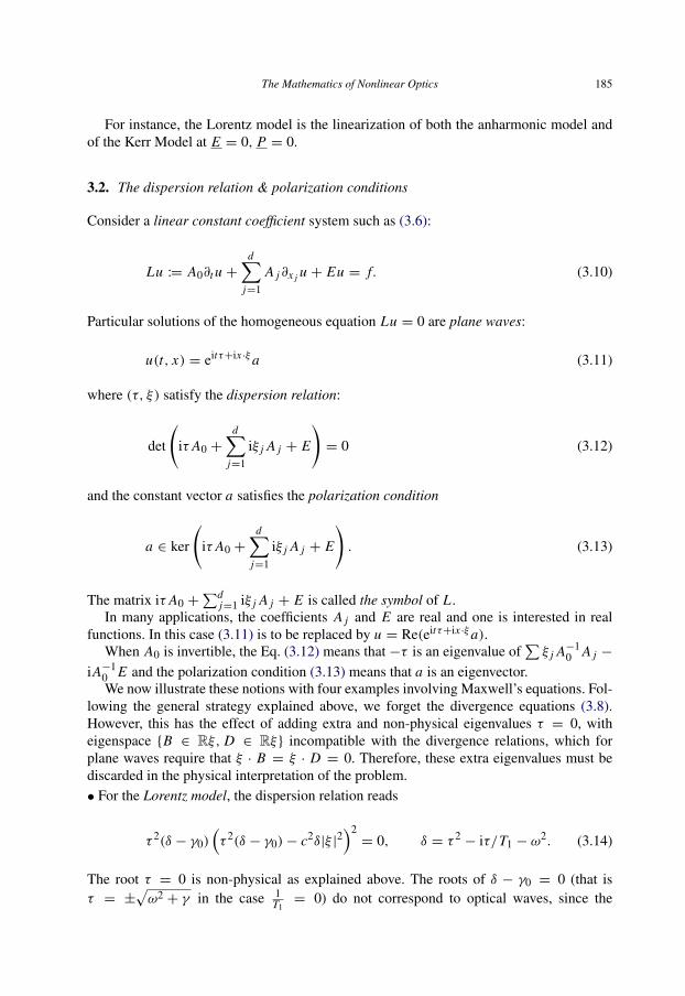
For instance, the Lorentz model is the linearization of both the anharmonic model andof the Kerr Model at E = 0, P = 0.
3.2. The dispersion relation & polarization conditions
Consider a linear constant coefficient system such as (3.6):
Lu := A0∂t u +d∑
j=1
A j∂x j u + Eu = f. (3.10)
Particular solutions of the homogeneous equation Lu = 0 are plane waves:
u(t, x) = eitτ+ix ·ξa (3.11)
where (τ, ξ) satisfy the dispersion relation:
det
(iτ A0 +
d∑j=1
iξ j A j + E
)= 0 (3.12)
and the constant vector a satisfies the polarization condition
a ∈ ker
(iτ A0 +
d∑j=1
iξ j A j + E
). (3.13)
The matrix iτ A0 +∑d
j=1 iξ j A j + E is called the symbol of L .In many applications, the coefficients A j and E are real and one is interested in real
functions. In this case (3.11) is to be replaced by u = Re(eitτ+ix ·ξa).When A0 is invertible, the Eq. (3.12) means that −τ is an eigenvalue of
∑ξ j A−1
0 A j −
iA−10 E and the polarization condition (3.13) means that a is an eigenvector.We now illustrate these notions with four examples involving Maxwell’s equations. Fol-
lowing the general strategy explained above, we forget the divergence equations (3.8).However, this has the effect of adding extra and non-physical eigenvalues τ = 0, witheigenspace {B ∈ Rξ, D ∈ Rξ} incompatible with the divergence relations, which forplane waves require that ξ · B = ξ · D = 0. Therefore, these extra eigenvalues must bediscarded in the physical interpretation of the problem.• For the Lorentz model, the dispersion relation reads
τ 2(δ − γ0)(τ 2(δ − γ0)− c2δ|ξ |2
)2= 0, δ = τ 2
− iτ/T1 − ω2. (3.14)
The root τ = 0 is non-physical as explained above. The roots of δ − γ0 = 0 (that isτ = ±
√ω2 + γ in the case 1
T1= 0) do not correspond to optical waves, since the

186 G. Metivier
corresponding waves propagate at speed 0 (see Section 5). The optical plane waves areassociated with roots of the third factor. They satisfy
c2|ξ |2 = τ 2 (1+ χ(τ )) , χ(τ ) =
γ0
ω2 + iτ/T1 − τ 2 . (3.15)
For ξ 6= 0, they have multiplicity two and the polarization conditions are
E ∈ ξ⊥, P = ε0χ(τ )E, B = −ξ
τ× E . (3.16)
• Consider the two level Maxwell–Bloch equations. The linearized equations aroundE = B = P = 0 and N = N0 > 0 read (in suitable units)
∂t B + curlE = 0, ∂t E − curlB = −∂t P,
ε∂2t P +�2 P = γ1 N0 E, ∂t N = 0.
(3.17)
This is the Lorentz model with coupling constant γ = γ1 N0, augmented by the equation∂t N = 0. Thus we are back to the previous example.
• For crystal optics, in units where c = 1, the plane wave equations reads{τ E − ε−1(ξ × B) = 0,τ B + ξ × E = 0.
(3.18)
In coordinates where ε is diagonal with diagonal entries α1 > α2 > α3, the dispersionrelation read
τ 2(τ 4−9(ξ)τ 2
+ |ξ |28(ξ))
(3.19)
with {9(ξ) = (α1 + α2)ξ
23 + (α2 + α3)ξ
21 + (α3 + α1)ξ
22 ,
8(ξ) = α1α2ξ23 + α2α3ξ
21 + α3α1ξ
22 .
For ξ 6= 0, τ = 0 is again a double eigenvalue. The non-vanishing eigenvalues are solutionsof a second order equation in τ 2, of which the discriminant is
92(ξ)− 4|ξ |28(ξ) = P2+ Q2
with
P = (α1 − α2)ξ23 + (α3 − α2)ξ
21 + (α3 − α1)ξ
22 ,

The Mathematics of Nonlinear Optics 187
Q = 2(α1 − α2)12 (α1 − α3)
12 ξ3ξ2.
For a bi-axial crystal, ε has three distinct eigenvalues. For general frequency ξ , P2+Q2
6=
0 and there are four simple eigenvalues,± 12
(9 ±
(P2+ Q2
) 12
) 12
. There are double roots
exactly when P2+ Q2
= 0, that is when
ξ2 = 0, α1ξ23 + α3ξ
21 = α2(ξ
21 + ξ
23 ) = τ
2. (3.20)
This is an example where the multiplicities of the eigenvalues change with ξ .
• Consider the linearized Maxwell–Bloch equations around E = B = 0 and ρ equal to thefundamental state, i.e. the eigenprojector associated with the smallest eigenvalue ω1 of �.In appropriate units, they read∂t B + curl E = 0,
∂t E − curl B − itr (0[�, ρ])+ itr (0(E · G)) = 0,∂tρ + i[�, ρ] − iE · G = 0,
(3.21)
with G := [0, ρ]. The general expression of the dispersion relation is not simple, onereason for that is the lack of isotropy of the general model shown above. To simplify, weassume that the fundamental state is simple, that � is diagonal with entries α j and wedenote by ω j the distinct eigenvalues of �, with ω1 = α1. Then G has the form
G =
0 −01,2 . . .
02,1 0 . . ....
... 0
.Assume that the model satisfies the following isotropy condition: for all ω j > ω1:∑
{k:αk=ω j }
(E · 01,k)0k,1 = γ j E (3.22)
with γ j ∈ C. Then the optical frequencies satisfy
|ξ |2 = τ 2(1+ χ(τ )), χ(τ ) =∑
2Reγ j (ω j − ω1)+ iτ Imγ j
(ω j − ω1)2 − τ 2 (3.23)
and the associated polarization conditions are
E ∈ ξ⊥, B = −ξ
τ× E, ρ1,k = ρk,1 =
E · 01,k
αk − α1 − τ(3.24)
with the other entries ρ j,k equal to 0.

188 G. Metivier
3.3. Existence and stability
The equations presented in Section 2 fall into the category of symmetric hyperbolic sys-tems. More precisely they satisfy the following condition:
DEFINITION 3.1 (Symmetry). A system (3.1) is said to be symmetric hyperbolic in thesense of Friedriechs, if there exists a matrix S(a, u) such that
– it is a C∞ function of its arguments;– for all j , a and u, the matrices S(a, u)A j (a, u) are self-adjoint and, in addition,
S(a, u)A0(a, u) is positive definite.
The Cauchy problem consists of solving the equation (3.1) together with the initial con-dition
u|t=0 = h. (3.25)
The first basic result of the theory is the local existence of smooth solutions:
THEOREM 3.2 (Local Existence). Suppose that the system (3.1) is symmetric hyperbolic.Then for s > d
2 + 1, h ∈ H s(Rd) and a ∈ C0([0; T ]; H s(Rd)) such that ∂t a ∈C0([0; T ]; H s−1(Rd)), there is T ′ > 0, T ′ ≤ T , which depends only on the norms of a,∂t a and h, such that the Cauchy problem has a unique solution u ∈ C0([0; T ′]; H s(Rd)).
In the semi-linear case, that is when the matrices A j do not depend on u, the limitinglower value for the local existence is s > d
2 :
THEOREM 3.3. Consider the semi-linear system (3.4) assumed to be symmetric hyper-bolic. Suppose that a ∈ C0([0; T ]; Hσ (Rd)) is such that ∂t a ∈ C0([0; T ]; Hσ−1(Rd))
where σ > d2 + 1. Then, for d
2 < s ≤ σ , h ∈ H s(Rd) and b ∈ C0([0; T ]; H s(Rd)), thereis T ′ > 0, T ′ ≤ T such that the Cauchy problem with initial data h has a unique solutionu ∈ C0([0; T ′]; H s(Rd)).
As it is important for understanding the remaining part of these notes we will give themain steps in the proof of this important result. The analysis of linear symmetric hyperbolicproblems goes back to [50,51]. For the nonlinear version we refer to [106,103,66,123].
PROOF (Scheme of the proof). Solutions can be constructed through an iterative schemeA0(a, un)∂t un+1 +
d∑j=1
A j (a, un)∂x j un+1 = F(a, un),
un+1|t=0 = h.
(3.26)
There are four steps:1 - [Definition of the scheme.] Prove that if un ∈ C0([0; T ]; H s(Rd)) and ∂t un ∈
C0([0; T ]; H s−1(Rd)), the system has a solution un+1 with the same smoothness;
The Mathematics of Nonlinear Optics 189
2 - [Boundedness in high norm.] Prove that there is T ′ > 0 such that the sequence isbounded in C0([0; T ′]; H s(Rd)) and C1([0; T ′]; H s−1(Rd)).
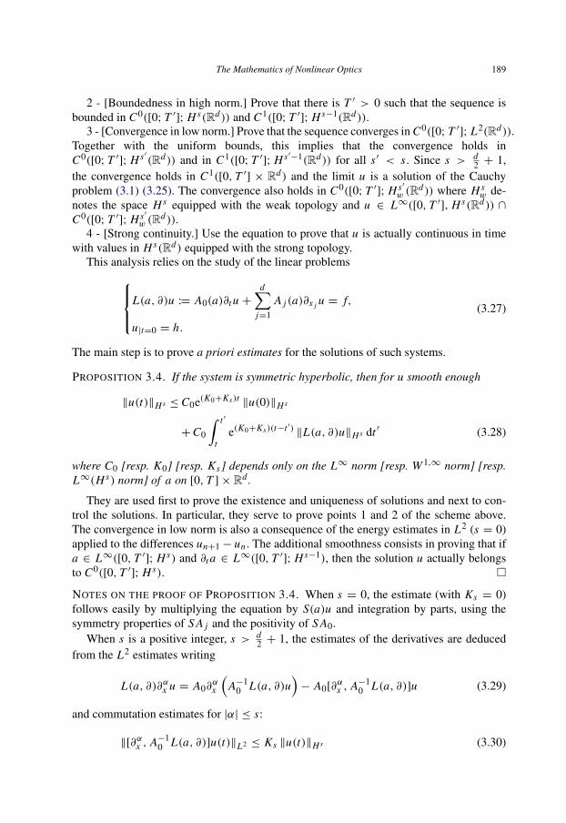
3 - [Convergence in low norm.] Prove that the sequence converges in C0([0; T ′]; L2(Rd)).Together with the uniform bounds, this implies that the convergence holds inC0([0; T ′]; H s′(Rd)) and in C1([0; T ′]; H s′−1(Rd)) for all s′ < s. Since s > d
2 + 1,the convergence holds in C1([0, T ′] × Rd) and the limit u is a solution of the Cauchyproblem (3.1) (3.25). The convergence also holds in C0([0; T ′]; H s′
w (Rd)) where H sw de-
notes the space H s equipped with the weak topology and u ∈ L∞([0, T ′], H s(Rd)) ∩
C0([0; T ′]; H s′w (Rd)).
4 - [Strong continuity.] Use the equation to prove that u is actually continuous in timewith values in H s(Rd) equipped with the strong topology.
This analysis relies on the study of the linear problemsL(a, ∂)u := A0(a)∂t u +d∑
j=1
A j (a)∂x j u = f,
u|t=0 = h.
(3.27)
The main step is to prove a priori estimates for the solutions of such systems.
PROPOSITION 3.4. If the system is symmetric hyperbolic, then for u smooth enough
‖u(t)‖H s ≤ C0e(K0+Ks )t ‖u(0)‖H s
+C0
∫ t ′
te(K0+Ks )(t−t ′)
‖L(a, ∂)u‖H s dt ′ (3.28)
where C0 [resp. K0] [resp. Ks] depends only on the L∞ norm [resp. W 1,∞ norm] [resp.L∞(H s) norm] of a on [0, T ] × Rd .
They are used first to prove the existence and uniqueness of solutions and next to con-trol the solutions. In particular, they serve to prove points 1 and 2 of the scheme above.The convergence in low norm is also a consequence of the energy estimates in L2 (s = 0)applied to the differences un+1− un . The additional smoothness consists in proving that ifa ∈ L∞([0, T ′]; H s) and ∂t a ∈ L∞([0, T ′]; H s−1), then the solution u actually belongsto C0([0, T ′]; H s). �
NOTES ON THE PROOF OF PROPOSITION 3.4. When s = 0, the estimate (with Ks = 0)follows easily by multiplying the equation by S(a)u and integration by parts, using thesymmetry properties of S A j and the positivity of S A0.
When s is a positive integer, s > d2 + 1, the estimates of the derivatives are deduced
from the L2 estimates writing
L(a, ∂)∂αx u = A0∂αx
(A−1
0 L(a, ∂)u)− A0[∂
αx , A−1
0 L(a, ∂)]u (3.29)
and commutation estimates for |α| ≤ s:
‖[∂αx , A−10 L(a, ∂)]u(t)‖L2 ≤ Ks ‖u(t)‖H s (3.30)

190 G. Metivier
where Ks depends only on the H s norm of a(t).The bound (3.30) follows from two classical nonlinear estimates which are recalled in
the lemma below.
LEMMA 3.5. For σ > d2 ,
(i) Hσ (Rd) is a Banach algebra embedded in L∞(Rd).(ii) For u ∈ Hσ−l(Rd) and v ∈ Hσ−m(Rd) with l ≥ 0, m ≥ 0 and l + m ≤ σ , the
product uv belongs to Hσ−l−m(Rd) ⊂ L2(Rd).(iii) For s > d
2 and F a smooth function such that F(0) = 0, the mapping u 7→ F(u)is continuous from H s(Rd) into itself and maps bounded sets to bounded sets.
Indeed, the commutator [∂αx , A−10 L(a, ∂)]u is a linear combination of terms
∂γx ∂xk A j (a)∂
βx ∂x j u, |β| + |γ | ≤ |α| − 1. (3.31)
Noticing that A j (a(t)) ∈ H s(Rd), and applying (ii) of the lemma with σ = s − 1, yieldsthe estimate (3.30). �
REMARK 3.6. The use of L2 based Sobolev spaces is well adapted to the framework ofsymmetric systems, but it is also dictated by the consideration of multidimensional prob-lems (see [112]).
Besides the existence statement, which is interesting from a mathematical point of view,the proof of Theorem 3.2 contains an important stability result:
THEOREM 3.7 (Local stability). Under assumptions of Theorem 3.2, if u0 ∈
C0([0, T ], H s(Rd)) is a solution of (3.1), then there exists δ > 0 such that for all initialdata h such that ‖h − u0(0)‖H s ≤ δ, the Cauchy problem with initial data h has a uniquesolution u ∈ C0([0, T ], H s(Rd)). Moreover, for all t ∈ [0, T ], the mapping h 7→ u(t)defined in this way, is Lipschtiz continuous in the H s−1 norm and continuous in the H s′
norm, for all s′ < s, uniformly in t.
3.4. Continuation of solutions
Uniqueness in Theorem 3.2 allows one to define the maximal interval of existence ofa smooth solution: under the assumptions of this theorem, let T ∗ be the supremum ofT ′ ∈ [0, T ] such that the Cauchy problem has a solution in C0([0, T ′]; H s(Rd)). By theuniqueness, this defines a (unique) solution u ∈ C0([0, T ∗[; H s(Rd)). With this definition,Theorem 3.2 immediately implies the following.
LEMMA 3.8. It T ∗ < T , then
supt∈[0,T ∗[
‖u(t)‖H s = +∞.
We mention here that a more precise result exists (see e.g. [103]):

The Mathematics of Nonlinear Optics 191
THEOREM 3.9. It T ∗ < T , then
supt∈[0,T ∗[
‖u(t)‖L∞ + ‖∇x u(t)‖L∞ = +∞.
We also deduce from Theorem 3.2 two continuation arguments based on a priori esti-mates:
LEMMA 3.10. Suppose that there is a constant C such that if T ′ ∈ ]0, T ] and u ∈C0([0, T ′]; H s) is solution of the Cauchy problem for (3.1) with initial data h ∈ H s ,then it satisfies for t ∈ [0, T ′]:
‖u(t)‖H s ≤ C. (3.32)
Then, the maximal solution corresponding to the initial data h is defined on [0, T ] andsatisfies (3.32) on [0, T ].
LEMMA 3.11. Suppose that there is are constants C and C ′ > C ≥ ‖h‖H s such that ifu ∈ C0([0, T ′]; H s) is solution of the Cauchy problem for (3.1) with initial data h ∈ H s
the following implication holds:
supt∈[0,T ′]
‖u(t)‖H s ≤ C ′ ⇒ supt∈[0,T ′]
‖u(t)‖H s ≤ C. (3.33)
Then, the maximal solution is defined on [0, T ] and satisfies (3.32) on [0, T ].
3.5. Global existence
As mentioned in the introduction, the general theorem of local existence is of little use forhigh frequency initial data, since the time of existence depends on high regularity normsand thus may be very small. In the theory of hyperbolic equations, there is a huge literatureon global existence and stability results. We do not mention here the results which concernsmall data (see e.g. [66] and the references therein), since the smallness is again measuredin high order Sobolev spaces and thus is difficult to apply to high frequency solutions.
There is another class of classical global existence theorems of weak or energy solutionsfor hyperbolic maximal dissipative equations, which use only the conservation or dissipa-tion of energy and a weak compactness argument (see e.g. [99] and Section 7.6.4 below.)
In this section, we illustrate with an example another approach which is better adaptedto our context. Indeed, for most of the physical examples, there are conserved (or dissi-pated) quantities, such as energies. These provide a priori estimates that are valid for alltime, independently of the size of the data. The problem is to use this particular additionalinformation to improve the general analysis and eventually arrive at global existence.
The case of two levels Maxwell–Bloch equations has been studied in [42]. Their re-sults have been extended to general Maxwell–Bloch equations (2.22) in [46] and to theanharmonic model (2.20) in [77] (see also [83] for Maxwell’s equations in a ferromag-netic medium). In the remaining part of this section, we present the example of two level

192 G. Metivier
Maxwell–Bloch equations. Recall the equations from Section 2:∂t B + curl E = 0,∂t (E + P)− curl B = 0,∂t P +�2 P = γ1 N E,∂t N = −γ2∂t P · E,
(3.34)
together with the constraints
div (E + P) = div B = 0. (3.35)
Recall that N is the difference between the number of electrons in the excited state and inthe ground state per unit of volume. N0 is the equilibrium value of N . This system can bewritten as a first order semi-linear symmetric hyperbolic system for
U = (B, E, P, ∂t P, N − N0). (3.36)
Since the system is semi-linear, with matrices A j that are constant, the local existencetheorem proves that the Cauchy problem is locally well-posed in H s(R3) for s > 3
2 , seeTheorem 3.3. The special form of the system implies that the maximal time of existence isT ∗ = +∞:
THEOREM 3.12. If s ≥ 2 and the initial data U (0) ∈ H s(R3) satisfies (3.35), then theCauchy problem for (3.34) has a unique solution U ∈ C0([0,+∞[; H s(R3)), which sat-isfies (3.35) for all time.
NOTES ON THE PROOF (see [42]). The total energy
E = N0 ‖B‖2L2 + N0 ‖E‖
2L2 +
�2
γ1‖P‖2L2 +
1γ1‖∂t P‖2L2 +
1γ2‖N − N0‖
2L2
is conserved, proving that U remains bounded in L2 for all time.
There is also a pointwise conservation of
1γ1|∂t P|2 +
�2
γ1|P|2 +
1γ2|N |2
proving that P , ∂t P and N remain bounded in L∞ for all time.
The H1 estimates are obtained by differentiating the equations with respect to x :∂t∂B + curl ∂E = 0,∂t∂E − curl ∂B = −∂t∂P,∂t∂P +�2∂P = γ1∂(N E),∂t∂N = −γ2∂(∂t P · E).

The Mathematics of Nonlinear Optics 193
Then
E1 = ‖∂B‖2L2 + ‖∂E‖2L2 +�2
γ1‖∂P‖2L2 +
1γ1‖∂t∂P‖2L2 +
1γ2‖∂N‖2L2
satisfies
∂t E1 = 2∫8dx
with
8=−(∂Q)∂E + ∂(N E)∂Q − ∂(QE)∂N
=−(∂Q)∂E + N∂E∂Q − ∂N Q∂E,
with Q = ∂t P . Thus, using the known L∞ bounds for N and Q, implies that
∂e E1 ≤ C E1
implying that E1(t) ≤ eCt E1(0) for all time.The estimate of the second derivatives is more subtle, but follows the same ideas: use
the known L2, L∞ and H1 bounds to obtain H2 estimates valid for all time. For the detailswe refer to [42]. �
Using the a priori H1 bounds, it is not difficult to prove the global existence of globalH1 solutions (see [42]):
THEOREM 3.13. For arbitrary U (0) ∈ H1(R3) satisfying (3.35) and such that(P(0), ∂t P(0), N (0)) ∈ L∞(R3), there is a unique global solution U such that for allT > 0,U ∈ L∞([0, T ]; H1(R3)) and (P, ∂t P, N ) ∈ L∞([0,+∞[×R3).
3.6. Local results
A fundamental property of hyperbolic systems is that they reproduce the physical ideathat waves propagate at a finite speed. Consider solutions of a symmetric hyperboliclinear equation
L(a, ∂)u := A0(a)∂t u +d∑
j=1
A j (a)∂x j u + E(a)u = f (3.37)
on domains of the form:
� = {(t, x) : t ≥ 0, |x | + tλ∗ ≤ R}. (3.38)
Let ω = {x : |x | ≤ R}. One has the following result.
PROPOSITION 3.14 (Local uniqueness). There is a real valued function λ∗(M), which de-pends only the matrices A j in the principal part, such that if λ∗ ≥ λ∗(M), a is Lipschitz

194 G. Metivier
continuous on � with |a(t, x)| ≤ M on �, u ∈ H1(�) satisfies (3.37) on � with f = 0and u|t=0 = 0 on ω, then u = 0 on �.
PROOF. By Green’s formula
0= 2Re∫�
e−γ t Lu · u dtdx
=
∫�
e−γ t (γ A0u − K u) · u dtdx
+
∫6
e−γ t L(a, ν)u · u d6
where K = ∂t A0(a) +∑∂x j A j (a), 6 = {λ∗t + |x | = R} and L(a, ν) =
∑ν j A j is the
value of L in the direction ν = (ν0, . . . , νd), which is the exterior normal to �. Becauseν is proportional to (λ∗, x1|x |, . . . , xd/|x |), if λ∗ is large enough, the matrix L(a, ν) isnonnegative. More precisely, this condition is satisfied if
λ∗ ≥ λ∗(M) = sup|a|≤M
sup|ξ |=1
supp|λp(a, ξ)| (3.39)
where the λp(a, ξ) denote the eigenvalues of A0(a)−1∑dj=1 ξ j A j (a).
If γ is large enough, the matrix γ A0 − K is positive definite, and the energy identityabove implies that u = 0 on �. �
This result implies that the solution u of (3.37) is uniquely determined in � by the val-ues of the source term f on � and the values of the initial data on ω. One says that � iscontained in the domain of determinacy of ω.
The proposition can be improved, giving the optimal domain of determinacy � associ-ated to an initial domain ω, see [93,96,84] and the references therein.
On domains �, one uses the following spaces:
DEFINITION 3.15. We say that u defined on � is continuous in time with values in L2 ifits extension by 0 outside � belongs to C0([0, T0]; L2(Rd)); for s ∈ N, we say that u iscontinuous with values in H s if the derivatives ∂αx u for |α| ≤ s are continuous in time withvalues in L2. We denote these spaces by C0 H s(�).
Proposition 3.14 extends to semi-linear equations, as the domain � does not depend onthe source term f (u). The energy estimates can be localized on �, using integration byparts on �, and Theorem 3.3 can be extended as follows:
THEOREM 3.16. Consider the semi-linear system (3.4) assumed to be symmetric hyper-bolic. Suppose that a ∈ C0 Hσ (�) is such that ∂t a ∈ C0 Hσ−1(�) where σ > d
2 + 1and ‖a‖L∞(�) ≤ M. Then, for d
2 < s ≤ σ , h ∈ H s(ω) and b ∈ C0 H s(�), thereexists T > 0, such that the Cauchy problem with initial data h has a unique solutionu ∈ C0 H s(� ∩ {t ≤ T }).
For quasi-linear systems (3.1), the situation is more intricate since then the eigenval-ues depend on the solution itself, so that λ∗(M) in (3.39) must be replaced by a function

The Mathematics of Nonlinear Optics 195
λ∗(M,M ′) which dominates the eigenvalues of A0(a, u)−1∑ ξ j A j (a, u) when |a| ≤ Mand |u| ≤ M ′. Note that λ∗(M,M ′) is a continuous increasing function of M ′, so that ifλ∗ > λ∗(M,M ′) then λ∗ ≥ λ∗(M,M ′′) for a M ′′ > M ′.
THEOREM 3.17. Suppose that the system (3.1) is symmetric hyperbolic. Fix M, M ′ ands > d
2 + 1. Let � denote the set (3.38) with λ∗ > λ(M,M ′). Let h ∈ H s(Rd) anda ∈ C0 H s(�) be such that ‖h‖L∞(ω) ≤ M ′, ∂t a ∈ C0 H s−1(�) and ‖a‖L∞(�) ≤ M. Thenthere exists T > 0, such that the Cauchy problem has a unique solution u ∈ C0 H s(� ∩
{t ≤ T }).
4. Equations with parameters
A general feature of problems in optics is that very different scales are present: for in-stance, the wavelength of the light beam is much smaller than the length of propagation,the length of the beam is much larger than its width. Many models (Lorentz, anharmonic,Maxwell–Bloch, Euler–Maxwell) contain many parameters, which may be large or small.In applications to optics, we are facing two opposite requirements:
– optics concerned with high frequency regimes, that is functions with Fourier trans-forms localized around large values of the wave number ξ ;
– we want to consider waves with large enough amplitude so that nonlinear effects arepresent in the propagation of the main amplitude.
Obviously, large frequencies and not too small amplitudes are incompatible with uni-form H s bounds for large s. Therefore, a direct application of Theorem 3.2 for highlyoscillatory but not small data, yields existence and stability for t ∈ [0, T ] with T verysmall, and often much smaller than any relevant physical time in the problem. This is why,one has to keep track of the parameters in the equations and to look for existence or stabilityresults which are independent of these parameters. In this section, we give two examplesof such results, which will be used for solving envelope equations and proving the stabilityof approximate solutions, respectively.
Note that all the results given in this section have local analogues on domains of deter-minacy, in the spirit of Section 3.6.
4.1. Singular equations
We start with two examples which will serve as a motivation:
– The Lorentz model (2.11) (see also (2.21) and (2.24)) contains a large parameter ωin front of the zeroth order term. Similarly, Bloch’s equations (2.22) contain a smallparameter ε in front of the derivative ∂t .
– To take into account the multiscale character of the phenomena, one can introduceexplicitly the fast scales and look for solutions of (3.1) of the form
u(t, x) = U (t, x, ϕ(t, x)/ε) (4.1)

196 G. Metivier
where ϕ is valued in Rm , and U is a function of (t, x) and additional independent variablesy = (y1, . . . , ym).
Both cases lead to equations of the form
A0(a, u)∂t u +d∑
j=1
A j (a, u)∂x j u +1ε
L(a, u, ∂x )u = F(a, u) (4.2)
with possibly an augmented number of variables x j and an augmented number of parame-ters a. In (4.2)
L(a, u, ∂x ) =
d∑j=1
L j (a, u)∂x j + L0(a, u). (4.3)
We again assume that F(0, 0) = 0. This setting occurs in many other fields, in particularin fluid mechanics, in the study of low Mach number flows (see e.g. [86,87,115]) or in theanalysis of rotating fluids.
Multiplying by a symmetrizer S(a, u), if necessary, we assume that the following con-dition is satisfied:
ASSUMPTION 4.1 (Symmetry). For j ∈ {0, . . . , d}, the matrices A j (a, u) are self-adjointand in addition A0(a, u) is positive definite.
For all j ∈ {1, . . . ,m} the matrices L j (a, u) are self-adjoint and L0(a, u) is skew ad-joint.
Theorem 3.2 implies that the Cauchy problem is locally well-posed for systems (4.2),but the time of existence given by this theorem in general shrinks to 0 as ε tends to 0. Tohave a uniform interval of existence, additional conditions are required. We first give twoexamples, before giving hints for a more general discussion.
4.1.1. The weakly nonlinear case Consider a system (4.2) where all the coefficientsA j and Lk are functions of (εa, εu). Expanding Lk(εa, εu) = Lk + ε Ak(ε, a, u) yieldssystems with the following structure:
A0(εa, εu)∂t u +d∑
j=1
A j (a, u)∂x j u +1ε
L(∂x )u = F(a, u) (4.4)
where L has the form (4.3) with constant coefficients L j . We still assume that the symme-try Assumption 4.1 is satisfied and F(0, 0) = 0. The matrices A j and F could also dependsmoothly on ε, but for simplicity we forget this easy extension.
THEOREM 4.2 (Uniform local Existence). Suppose that h ∈ H s(Rd) and a ∈
C0([0; T ]; H s(Rd))∩C1([0; T ]; H s−1(Rd)), where s > d2 + 1. Then, there exists T ′ > 0
such that, for all ε ∈]0, 1], the Cauchy problem for (4.4) with initial data h has a uniquesolution u ∈ C0([0; T ′]; H s(Rd)).

The Mathematics of Nonlinear Optics 197
SKETCH OF PROOF. Consider the linear version of the equation
Lε(a, ∂)u := A0(εa)∂t u +d∑
j=1
A j (a)∂x j u +1ε
L(∂x )u = f. (4.5)
Thanks to the symmetry, the L2 estimate is found immediately. The following expressionholds
‖u(t)‖L2 ≤ C0eK0t‖u(0)‖L2
+C0
∫ t ′
teK0(t−t ′)
‖Lε(a, ∂)u‖H s dt ′ (4.6)
with C0 [resp. K0] depending only on the L∞ norm [resp. W 1,∞ norm] of εa.Next, one commutes A−1
0 Lε with the derivatives ∂αx as in (3.29). The key new obser-vation is that the derivatives ∂αx (ε
−1 A−10 (εa)L j ) are bounded with respect to ε, as well as
the derivatives ∂αx (A−10 (εa)A j (a)). The precise estimate is that for s > d
2 + 1, there is Ks
which depends only on the H s norm of a(t), such that for |α| ≤ s, there holds
‖[∂αx , A−10 Lε(a, ∂)]u(t)‖L2 ≤ Ks ‖u(t)‖H s . (4.7)
From here, the proof is as in the nonsingular case. �
4.1.2. The case of prepared data We relax here the weakly nonlinear dependence of thecoefficient A0 and consider a system:
A0(a, u)∂t u +d∑
j=1
A j (a, u)∂x j u +1ε
L(∂x )u = F(a, u) (4.8)
and its linear version
Lε(a, ∂)u := A0(a)∂t u +d∑
j=1
A j (a)∂x j u +1ε
L(∂x )u = f (4.9)
where L has constant coefficients L j . We assume that the symmetry Assumption 4.1 issatisfied and F(0, 0) = 0.
The commutators [∂αx , ε−1 A−1
0 (a)Lε] are of order ε−1, so that the method of proof ofTheorem 4.2 cannot be used anymore. Instead, one can use the following path: the commu-tators [∂x , ε
−1 L] are excellent, since they vanish identically. Thus one can try to commute∂αx and Lε(a) directly. However, this commutator contains terms ∂α−βx A0(a)∂t∂
βx u and
hence the mixed time-space derivative ∂t∂βx u. One cannot use the equation to replace ∂t u
by the spatial derivative, since this would reintroduce singular terms. Therefore, to close theestimate one is led to estimate all the derivatives ∂α0
t ∂αx u. Then, the commutator argument

198 G. Metivier
closes, yielding an existence result on a uniform interval of time, provided that the initialvalues of all the derivatives ∂α0
t ∂αx u are uniformly bounded. Let us proceed to the details.
For s ∈ N, introduce the space C H s([0, T ]×Rd) of functions u ∈ C0([0, T ]; H s(Rd))
such that for all k ≤ s, ∂kt u ∈ C0([0, T ]; H s−k(Rd)). It is equipped with the norm
‖u‖C H s = supt∈[0,T ]
|||u(t)|||s, |||u(t)|||s =s∑
k=0
‖∂kt u(t)‖H s−k (Rd ). (4.10)
For s > d2 , the space CHs is embedded in L∞. Therefore, the chain rule and Lemma 3.5
imply that for smooth F , such that F(0) = 0, the mapping u 7→ F(u) is continuous fromC H s into itself and maps bounded sets to bounded sets.
Moreover, the commutator [∂αt,x , Lε(a, ∂)]u is a linear combination of terms
∂γt,x A j (a)∂
βt,x u, (4.11)
with
0 ≤ |γ | − 1 ≤ s − 1, 0 ≤ |β| − 1, |γ | − 1+ |β| − 1 ≤ s − 1.
Since A j (a(t)) ∈ C H s , (ii) of Lemma 3.5 applied with σ = s − 1 implies for s > d2 + 1
the following commutator estimates∥∥[∂αt,x , Lε(a, ∂x )]u(t)∥∥
L2 ≤ C |||u(t)|||s (4.12)
where C depends on the norm |||a(t)|||s .For systems (4.9), the L2 energy estimates are again straightforward from the symmetry
assumption. Together with the commutator estimates above, they provide bounds for thenorms |||u(t)|||s , uniform and t and ε, provided that their initial values |||u(0)|||s are bounded.
The initial values ∂kt u(0) are computed by induction using the equation: for instance
∂t u|t=0 =−A−10 (a0, u0)(
d∑j=1
A j (a0, u0)∂x j u0 +1ε
L(∂x )u0 − F(a0, u0)
)(4.13)
where a0 = a|t=0 and u0 = u|t=0. In particular, for a fixed initial data u|t=0 = h, the term∂t u|t=0 is bounded independently of ε if and only if
L(∂x )h = 0. (4.14)
The analysis of higher order derivatives is similar. To simplify the notation, let ∂(k)udenote a product of derivatives of u of total order k:
∂α1u . . . ∂αp u with α j > 0 and |α1| + · · · + |αp| = k. (4.15)

The Mathematics of Nonlinear Optics 199
LEMMA 4.3. For s > (d + 1)/2 and k ∈ {0, . . . , s}, there are nonlinear functionalsFε
k (a, u), which are finite sums of terms
ε−l8(a, h)(∂(p)t,x a)(∂(p)x u), l ≤ k, p + q ≤ k (4.16)
with 8 smooth, such that for a ∈ C H s and h ∈ H s and all ε > 0, the local solution of theCauchy problem for (4.8) with initial data h belongs to C H s and
∂kt u = Fε
k (a, h). (4.17)
PROOF. For C∞ functions, (4.17) is immediate by induction on k. Lemma 3.5 impliesthat the identities extend to coefficients a ∈ C H s and u ∈ C0([0, T ′], H s), proving byinduction that ∂k
t u ∈ C0([0, T ′], H s−k). �
In particular, if u is a solution of (4.8) with initial data h, there holds
(∂kt u)|t=0 = Hε
k(a, h) := Fεk (a, h)|t=0 (4.18)
Note that Hεk is singular as ε→ 0, since in general it is of order ε−k .
THEOREM 4.4. Suppose that s > d2 + 1 and a ∈ C H s([0, T ]×Rd) and h ∈ H s(Rd) are
such that the families Hεk(a, h) are bounded for ε ∈ ]0, 1].
Then, there exists T ′ > 0 such that for all ε ∈ ]0, 1] the Cauchy problem for (4.8) withinitial data h has a unique solution u ∈ C H s([0, T ′] × Rd).
SKETCH OF THE PROOF (See e.g. [11]). The assumption means that the initial norms|||u(0)|||s are bounded, providing uniform estimates of |||u(t)|||s for t ≤ T ′, for some T ′ > 0independent of ε. This implies that the local solution can be continued up to time T ′. �
The data which satisfy the condition for Hεk(a, h) are often called prepared data. The
first condition (4.14) is quite explicit, but the higher order conditions are less explicit, andthe construction of prepared data is a nontrivial independent problem. However, there is aninteresting application of Theorem 4.4 when the wave is created not by an initial data butby a forcing term which vanishes in the past: consider the problem
A0(a, u)∂t u +d∑
j=1
A j (a, u)∂x j u +1ε
L(∂x )u = F(a, u)+ f (4.19)
with F(a, 0) = 0. (In the notations of (4.8), this means that f = F(a, 0)). We con-sider f as one of the parameters entering the equation. We assume that f is given inC H s([0, T ] × Rd) and vanishes at order s on t = 0:
∂kt f|t=0 = 0, k ∈ {0, . . . , s − 1}. (4.20)

200 G. Metivier
Then, one can check by induction, that for a vanishing initial data h = 0 the traces of thesolution vanish:
∂kt u|t=0 = 0, k ∈ {0, . . . , s}. (4.21)
Therefore:
THEOREM 4.5. Suppose that s > d2 + 1, a ∈ C H s([0, T ] × Rd) and f ∈ C H s([0, T ] ×
Rd) satisfies (4.20).Then, there exists T ′ > 0 such that for all ε ∈ ]0, 1] the Cauchy problem for (4.19) with
vanishing initial data has a unique solution u ∈ C H s([0, T ′] ×Rd) and u satisfies (4.21).
4.1.3. Remarks on the commutation method The proofs of Theorems 3.2, 4.2 and 4.4 arebased on commutation properties which strongly depend on the structure of the equation.In particular, it was crucial in (4.4) and (4.8) that the singular part L(∂x ) had constant co-efficients and that A0 depended on (εa, εu) in the former case. Without assuming maximalgenerality, we investigate here to what extent the commutation method can be extended tomore general equations (4.2) where L and A0 could also depend on a.
1. The principle of the method. Consider a linear equation L(t, x, ∂)u = f and assume thatthere is a good L2 energy estimate. We suppose that the coefficients are smooth functionsof a and that a is smooth enough. Consider a set of vector fields Z = {Z1, . . . , Zm}, whichwe want to commute with the equation. The commutation properties we use are of the form:
L(t, x, ∂)Z j = Z j L(t, x, D)+∑
R j,k Zk
with bounded matrices R j,k . The energy estimate is then applied to Z j u. However, onemust keep in mind that one could perform a change of variables u = V v or pre-multiplythe equation by a matrix before commuting with the Z j . This is equivalent to adding zeroorder terms to the Z j and looking for relations of the form
L(t, x, ∂)(Z j + B j ) = (Z j + C j )L(t, x, D)+∑
R j,k Zk + R j,0 (4.22)
with matrices B j and C j to be found, depending on a and its derivatives. Together with theL2 estimate, this clearly implies estimates of derivatives Z j1 . . . Z jm u, and knowing similarestimates for the right hand side f and the initial data.
2. Analysis of the commutation conditions. The operator L is split into a good part, thelinear combination of the Z j , and a bad or singular part:
L(t, x, ∂) =∑
A j (t, x)Z j +∑
Gk(t, x)Tk (4.23)
where the Tk are some other vector fields or singular terms which commute with the Z j .Only the commutation with terms Gk(t, x)Tk may cause problems, and the commutationconditions read
Z j (Gk) = Gk B j − C j Gk, (4.24)

The Mathematics of Nonlinear Optics 201
assuming that
the [Tk, B j ] are bounded. (4.25)
We now analyze the geometric implications of (4.24).
LEMMA 4.6. Suppose that the Gk are smooth matrices and Z is an integrable system ofvector fields. Then, locally, there are smooth matrices B j and C j satisfying (4.24), if andonly if there are smooth invertible matrices W and V , such that
∀ j,∀k, [Z j ,W Gk V ] = 0. (4.26)
In this case, for all η ∈ Rm , the rank of∑ηk Gk is constant along the integral leaves
of Z .
PROOF. If Gk = W Gk V , then
Z j (Gk) = W(
W−1(Z j W )Gk + Z(Gk)+ Gk Z j (V )V−1)
V .
Thus, if Z(Gk) = 0, then (4.24) holds with C j = W−1 Z j (W ) and B j = −Z j (V )V−1.
Conversely, one can assume locally that Z = {∂x1 , . . . , ∂xm } and prove the result byinduction on m. One determines locally W1 and V1 such that
∂x1 W1 = W1C1, ∂x1 V1 = −B1V1
and (4.24) implies ∂x1(W1G1V1) = 0. This finishes the proof when m = 1. When m > 1,let Gk = W1Gk V1. The commutation properties (4.24) are stable under such a transform:the Gk satisfy
∂x j Gk = Gk B j − C j Gk, (4.27)
with new matrices B j and C j , which vanish when j = 1. In particular, the Gk do notdepend on the first variable x1. Freezing the variable x1 at x1, we see that the commuta-tion relation (4.27) also holds with matrices B j and C j that are independent of x1. Fromhere, one can apply the induction hypothesis for the matrices Gk and the vector fields{∂x j , j ≥ 2} and find matrices W ′ and V ′, independent of x1, such that ∂x j (W
′Gk V ) = 0for j ≥ 2. The property (4.26) follows with W = W ′W1 and V = V1V ′.
The condition (4.26) implies that W (∑ηk Gk)V is independent of the variables
(x1, · · · , xm). In particular, its rank is constant when the other variables are fixed. �
REMARK 4.7. Suppose that l ≥ 2 and that G1 is invertible. Saying that the rankof
∑ηk Gk is independent of x , is equivalent to saying that the eigenvalues of∑
k≥2 ηk G−11 Gk are independent of x as well as their multiplicity.

202 G. Metivier
The next lemma shows that the commutation properties imply that the equation can betransformed to another equivalent equation with constant coefficients in the singular part.
LEMMA 4.8. (i) Suppose that G(a) is a smooth matrix of rank independent of a.Then, locally near any point a, there are smooth matrices W (a) and V (a) suchthat W (a)G(a)V (a) is constant.
(ii) Suppose that G0(a) and G(a) are smooth self-adjoint matrices with G0 positivedefinite, such that the eigenvalues of G−1
0 G(a) are independent of a. Then locally,there is a smooth matrix V (a) such that, with W = V−1G−1
0 , W (a)G0(a)V (a) andW (a)G(a)V (a) are constant.
In both cases, if a(t, x) is such that the Z j a are bounded, the commutation relations(4.24) are satisfied with bounded matrices B j and C j .
PROOF. (i) If the rank of G is constant equal toµ, in a neighborhood of a, there are smoothinvertible matrices W and V such that
W (a)G(a)V (a) =
(Id µ 0
0 0
).
(ii) Since G0 is positive definite and G is self-adjoint, G−10 G is diagonalizable. Since
the eigenvalues are constant, say equal to λ j , there is a smooth invertible matrix V such that
V−1(a)G−10 (a)G(a)V (a) = diag(λ j ). �
CONCLUSION 4.9. Lemmas 4.6 and 4.8 give key indications for the validity of the com-mutation method, applied to equations (4.23).
4.1.4. Application 1 Consider a system with coefficients depending smoothly on a
A0(a)∂t u +d∑
j=1
A j (a)∂x j u +1ε
B(a) = f. (4.28)
We assume that the matrices A j are self-adjoint with A0 positive definite and B(a) skew-adjoint.• For Z = {∂t , ∂x1 , . . . , ∂xd }, the commutation condition reads
the rank of B(a(t, x)) is independent of (t, x). (4.29)
Locally in a, this is equivalent to
there are smooth matrices W (t, x) and V (t, x) such that
W (t, x)B(a(t, x))V (t, x) is constant.(4.30)

The Mathematics of Nonlinear Optics 203
THEOREM 4.10. Suppose that a is a smooth function of (t, x). Under Assumption (4.30),there are energy estimates in the spaces C H s([0, T ] × Rd) for the solutions of (4.28), ofthe form
|||u(t)|||s ≤ CeK t|||u(0)|||s + C
∫ t
0eK (t−t ′)
||| f (t ′)|||sdt ′. (4.31)
• For Z = {∂x1 , . . . , ∂xd }, then ∂t becomes a “bad” vector field to be included in thesecond sum in (4.23). Following Remark 4.7, the condition reads
the eigenvalues of A−10 (a(t, x))B(a(t, x)) have constant
multiplicity.(4.32)
Locally in a, this is equivalent to
there is a smooth matrix V (t, x) such that
V−1(t, x)A−10 (a(t, x))B(a(t, x))V (t, x) is constant.
(4.33)
THEOREM 4.11. Suppose that a is a smooth function of (t, x). Under Assumption (4.33),there are energy estimates in the spaces C0([0, T ]; H s(Rd)) for the solutions of (4.28), ofthe form
‖u(t)‖s ≤ CeK t‖u(0)‖s + C
∫ t
0eK (t−t ′)
‖ f (t ′)‖sdt ′. (4.34)
4.1.5. Application 2 The following systems arise when one introduces fast scales (seeSection 7.4):
A0(a)∂t u +d∑
j=1
A j (a)∂x j u +1ε
(m∑
k=1
B j (a)∂θ j u + E(a)u
)= f. (4.35)
We assume that the matrices A j and Bk are self-adjoint with A0 is positive definite and E isskew symmetric. The additional variables θ = (θ1, . . . , θm) correspond to the fast variablesϕ/ε in (4.1). In this framework, functions are periodic in θ , and up to a normalization ofperiods, this means that θ ∈ Tm , T = R/(2πZ). There are other situations where systemsof the form (4.35) occur with no periodicity assumption in the variables θ j , for instance inthe low mach limit analysis Euler equation. The analysis can be adapted to some extent forthis case, but we do not investigate this question in detail here.
An important assumption is that
∂θ j a = 0, j ∈ {1, . . . ,m}. (4.36)

204 G. Metivier
In this case one can expand u and f in Fourier series in θ , and the Fourier coefficients uα ,α ∈ Zm are solutions of
A0(a)∂t uα +d∑
j=1
A j (a)∂x j uα +1ε
B(a, α)uα = fα (4.37)
where
B(a, η) =m∑
j=1
iη j B j (a)+ E(a). (4.38)
They are systems of the form (4.28). The conditions (4.29) (4.32) read
for all α ∈ Zm, the rank of B(a(t, x), α) is independent of (t, x), (4.39)
for all α ∈ Zm, the eigenvalues of A−10 (a(t, x))B(a(t, x), α)
have constant multiplicity,(4.40)
respectively. To get estimates uniform in α, we reinforce their equivalent formulation(4.29), (4.32) as follows:
ASSUMPTION 4.12. There are matrices W(t, x, α) and V(t, x, α) for α ∈ Zm , whichare uniformly bounded, as are their derivatives, with respect to (t, x), and a matrix B](α)
independent of (t, x) such that
W(t, x, α)B(a(t, x), α)V(t, x, α) = B](α). (4.41)
ASSUMPTION 4.13. There are matrices V(a(t, x), α) for α ∈ Zm , which are uniformlybounded, as are their derivatives, with respect to (t, x), and a matrix B](α) independent of(t, x) such that
V−1(t, x, α)A−10 (a(t, x))B(a(t, x), α)V(t, x, α) = B](α). (4.42)
Note that no smoothness in α is required in these assumptions.
THEOREM 4.14. Suppose that a is a smooth function of (t, x).
(i) Under Assumption 4.12 there are energy estimates in the spaces C H s([0, T ]×Rd×
Tm) for the solutions of (4.35)
|||u(t)|||s ≤ CeK t|||u(0)|||s + C
∫ t
0eK (t−t ′)
||| f (t ′)|||sdt ′. (4.43)

The Mathematics of Nonlinear Optics 205
(ii) Under Assumption 4.13, there are energy estimates in the spaces C0([0, T ]; H s(Rd×
Tm))
‖u(t)‖H s ≤ CeK t‖u(0)‖H s + C
∫ t
0eK (t−t ′)
∥∥ f (t ′)∥∥
H s dt ′. (4.44)
PROOF. The symmetry conditions immediately imply an L2 energy estimate for (4.37).The commutation properties are satisfied by ε−1 B(a, α) in the first case, and by{A0(a)∂t , ε
−1 B(a, α)} in the second case, providing estimates which are uniform in α.Moreover, the equation commutes with |α|, allowing for estimates of the ∂θ derivatives. �
REMARK 4.15. These estimates extend to equations
A0(a, εu)∂t u +d∑
j=1
A j (a, εu)∂x j u
+1ε
(m∑
k=1
B j (a, εu)∂θ j u + E(a, εu)u
)= f (4.45)
since all the additional commutators which involve εu are nonsingular. We stress thatthe conditions (4.41) or (4.42) are unchanged and bear on the coefficients A j (a, v) andB j (a, v) at v = 0. This yields existence theorems, which extend Theorem 4.4 for data pre-pared under Assumption 4.12, and Theorem 4.2 for general data under Assumption 4.13.We refer to [76] for details.
Next we give explicit conditions which ensure that the Assumptions are satisfied. Thefirst remark is trivial, but useful.
REMARK 4.16. If a(t, x) = a is constant, the Assumptions 4.12 and 4.13 are satisfied.
Next we consider the case where E = 0. Though the next proposition does not apply togeometric optics, it is natural and useful for other applications.
PROPOSITION 4.17. Suppose that E = 0 and there is δ > 0 such that for all a and η inthe sphere Sm−1, 0 is the unique eigenvalue of B(a, η) in the disk centered at 0 of radiusδ, and that its multiplicity is constant.
Then, the Assumption 4.12 is satisfied.
In Section 7 we will consider systems of the above form, such that the symmetric systemB(a(t, x), η) is hyperbolic in a direction η, which we can choose to be η = (1, 0, . . . , 0).We use the notations
η = (η1, η′), B(a, η) = η1 B1(a)+ B′(a, η′) (4.46)
and B1 is positive definite. Then the kernel of B(a(t, x), η) is nontrivial if and only if−η1 is an eigenvalue of B−1
1 B′(a(t, x), η′). In this case, a natural choice for a projectorP(t, x, η) on ker B is to consider the spectral projector, which is orthogonal for the scalarproduct defined by B1(a(t, x)). If −τ1 is not an eigenvalue, define P(t, x, η) = 0.

206 G. Metivier
PROPOSITION 4.18. With E = 0, assume that the symmetric symbol B is hyperbolic withtime-like co-direction η ∈ Rm
\ {0} and use the notations above. Then, locally in (t, x), theAssumption 4.12 is satisfied if
(i) for all η ∈ Rm the rank of B(a(t, x), η) is independent of (t, x),(ii) for all η ∈ Rm the projectors P(t, x, η) are smooth in (t, x), and the set{P( ·, , η)}{η∈Rm } is bounded in C∞.
In particular, the second condition is satisfied when the eigenvalues of B−11 B′(a(t, x), η′)
have their multiplicity independent of (t, x, η′), for η′ in the unit sphere.
PROOF. Condition (i) implies that for all η′, the eigenvalues of B−11 B′(a(t, x), η′), which
are all real by the hyperbolicity assumption, are independent of (t, x). By (ii), locally,there are smooth families of eigenvectors, which are orthonormal for the scalar prod-uct A0(a(t, x)), and uniformly bounded in C∞ independently of η′. This yields matricesV(t, x, η′) such that V( ·, η′) and V−1( ·, η′) are uniformly bounded in C∞ and
V−1(t, x, η′)B−11 a(t, x)B′(a(t, x), η′)V(t, x, η′) = diag(λ j (η
′)) := B[(η′).
Thus, with W = V−1 B1(a(t, x), η′) there holds
W(t, x, η′)B(a(t, x), η)V(t, x, η′) = iη1Id + B[(η′) := B[(η).
If the eigenvalues of B−11 B′(a(t, x), η′) have constant multiplicity in (t, x) and η′ 6= 0,
the spectral projectors are smooth in (t, x, η′) and homogeneous of degree 0 in η′,yielding (ii). �
Concerning Assumption 4.13, the same proof applied to iτ A0 + B(a, η) implies thefollowing:
PROPOSITION 4.19. With E = 0, the Assumption 4.12 is satisfied locally in (t, x) if:
(i) for all η ∈ Rm , the eigenvalues of A−10 (a(t, x))B(a(t, x), η) are independent of
(t, x),(ii) the spectral projectors of A−1
0 (a(t, x))B(a(t, x), η) are smooth in (t, x), andbelong to a bounded set in C∞ when η ∈ Rm .
In particular, the second condition is satisfied if the multiplicities of the eigenvalues ofA−1
0 (a(t, x))B(a(t, x, η)) are constant in (t, x, η) for η 6= 0.
In Section 7, we will use the following extensions:
PROPOSITION 4.20. Suppose that
B(a, η) =m∑
j=1
iη j B j (a) (4.47)
satisfies the assumption of Proposition 4.18 [resp. Proposition 4.19], and that there is am × m matrix M such that
B(a, η) = B(a,Mη). (4.48)

The Mathematics of Nonlinear Optics 207
Then, B satisfies the Assumption 4.12 [resp. Assumption 4.13].
There are analogous results when E 6= 0, but we omit them here for the sake of brevity.
4.2. Equations with rapidly varying coefficients
In this subsection we consider systems
A0(a, u)∂t u +d∑
j=1
A j (a, u)∂x j u +1ε
E(a)u = F(a, u) (4.49)
with the idea that a and u have rapid oscillations. More precisely, we assume thata ∈ L∞([0, T ] × Rd) and that its derivative satisfy 0 < |α| ≤ s:
ε|α|−1‖∂αt,x a‖L∞([0,T ]×Rd ). ≤ C1, (4.50)
Following the general existence theory, it is assumed that the integer s satisfies s > d2 + 1.
We suppose that u = 0 is almost a solution, that is that there is a real number M > 0 suchthat f = F(a, 0) is satisfied when |α| ≤ s
ε|α|‖∂αx f ε(t)‖L2(Rd ) ≤ εM C2. (4.51)
How large M must be chosen is part of the analysis. Similarly, we consider initial datawhich satisfy |α| ≤ s
ε|α|‖∂αx h‖L2(Rd ) ≤ εM C3. (4.52)
Note that these assumptions allow for families of data a, which have amplitude O(ε) atfrequencies |ξ | ≈ ε−1. In applications, a will be an approximate solution of the originalequation. The equation (4.49) with coefficients A j (a, 0) is the linearized equation nearthis approximate solution. Its well-posedness accounts for the stability of the approximatesolution and (4.49) can be regarded as an equation for a corrector.
We always assume that the equations are symmetric hyperbolic, that is that the matricesA j are self-adjoint with A0 positive definite and that E is skew symmetric.
THEOREM 4.21. Under the assumptions above, if M > 1 + d/2, there are ε1 > 0 andC4, depending only on the constants C1,C2,C3 and the coefficients A j and F, such thatfor ε ∈ ]0, ε1], the Cauchy problem for (4.49) with initial data h, has a unique solutionu ∈ C0([0, T ]; H s(Rd)) which satisfies
ε|α|‖∂αx u(t)‖L2(R) ≤ εM C4. (4.53)

208 G. Metivier
PROOF (See [59]). Write u = εMv, f = εM g and F(a, u) = f + εM G(a, u)v. Theequation for v reads
L(a, u, ∂)v := A0(a, u)∂tv +
d∑j=1
A j (a, u)∂x j v
+1ε
E(a)v − G(a, u)v = g. (4.54)
Introduce the norms
‖u‖H sε= sup|α|≤s
ε|α|‖∂αx u‖L2(Rd ). (4.55)
The main new ingredient is the weighted Sobolev inequality:
‖εMv‖L∞(Rd ) ≤ K εM− d2 ‖v‖H s−1
ε, (4.56)
‖εM∂xv‖L∞(Rd ) ≤ K εM− d2−1‖v‖H s
ε. (4.57)
Since M > d2 + 1, this implies that, if the H s
ε -norm of v is bounded by some constantC4, then the Lipschitz norms of the coefficients A j (a, εMv) are bounded by some constantindependent of C4, if ε is small enough.
Therefore the symmetry implies the following L2 estimate: there are constants C andK , which depend only on C1,C2,C3, and ε0 > 0 which depends in addition on C4, suchthat for ε ≤ ε0 and u satisfying (4.53) on [0, T ′], there holds for t ∈ [0, T ′]:
‖v(t)‖L2 ≤ CeK t‖v(0)‖L2 + C
∫ t
0eK (t−t ′)
∥∥L(a, u, ∂)v(t ′)∥∥
L2 dt ′. (4.58)
Next, one commutes the equation (pre-mulitplied by A−10 ) with the weighted derivatives
ε∂x j . One proves that for |α| ≤ s,∥∥∥[ε|α|∂αx , A−10 L(a, u, ∂)]v(t)
∥∥∥L2≤ K ‖v(t)‖H s
ε(4.59)
with K depending only on C1,C2,C3, provided that u satisfies (4.53) and ε ≤ ε0 whereε0 > 0 depends on C1,C2,C3 and C4. Indeed, by homogeneity, Lemma 3.5 implies thatfor σ > d
2 and l ≥ 0, m ≥ 0 with l + m ≤ σ , there holds
‖uv‖Hσ−l−mε
≤ Cε−d2 ‖u‖Hσ−l
ε‖v‖Hσ−m
ε. (4.60)
The commutator [ε|α|∂αx , A−10 A j∂ j ]v is a linear combination of terms
ε|α|∂β1
x a . . . ∂βq
x a∂α1
x u . . . ∂αp
x u∂γx v

The Mathematics of Nonlinear Optics 209
with 0 < |β j| ≤ s, |αk
| ≤ s, |γ | ≤ s and∑|β j| +∑|αk| + |γ | ≤ |α| + 1 ≤ s+ 1. These
terms belong to L2, as explained in the proof of Proposition 3.4. More precisely, using theassumptions (4.52) and (4.53) and the product rule (4.60), one obtains that the L2 norm ofsuch terms is bounded by
εµCCq1 C p
4 ‖v‖H sε
for some numerical constant C and
µ = |α| + pM −∑
(|β j| − 1)+ −
∑|αk| − |γ | − p
d
2.
If∑|β j| > 0, then
∑(|β j| − 1)+ ≤ (
∑|β j|) − 1 and µ = 0 when p = 0 and µ > 0
when p > 0 since M > d2 . If
∑|β j| = 0, then p > 0 and µ > 0 since M > d
2 + 1. Thisimplies that this term satisfies (4.59).
The commutator [ε|α|∂αx , ε−1 A−1
0 E]v is a linear combination of terms
ε|α|−1∂β1
x a . . . ∂βq
x a∂γx v
with∑|β j| + |γ | ≤ |α| ≤ s and
∑|β j| > 0. With (4.50), this term is also dominated as
in (4.59).Hence, there are constants C and K , which depend only on C1,C2,C3, and ε0 > 0
which depends in addition on C4, such that for ε ≤ ε0 and u satisfying (4.53) on [0, T ′],there holds for t ∈ [0, T ′]:
‖v(t)‖H sε≤ CeK t
‖v(0)‖H sε+ C
∫ t
0eK (t−t ′)
∥∥L(a, u, ∂)v(t ′)∥∥
H sε
dt ′. (4.61)
Choose C4 ≥ 2CeK T (C3 + C2) and ε0 accordingly, and assume that ε ≤ ε0. There-fore, (4.61) shows that if u satisfies ‖u(t)‖H s
ε≤ C4 on [0, T ′], then it also satisfies
‖u(t)‖H sε≤
12 C4 on this interval. By continuation, this implies that the local solution u
of (4.49) can be continued on [0, T ] and satisfies (4.53). �
5. Geometrical Optics
In this section we present the WKB method for two scale asymptotic expansions, applied tothe construction of high frequency wave packet solutions. This method rapidly leads to thegeometric optics equations, of which the main features are the eikonal equations, the po-larization conditions and the transport equation most often along rays. The formal asymp-totic solutions can be converted into approximate solutions by truncating the expansion.The next main step is to study their stability, with the aim of constructing exact solutionsclose to them. We first review the linear case and next we consider the general regime ofweakly nonlinear geometric optics where general results of existence and stability of oscil-lating solutions are available. The transport equations are in general nonlinear. In particularBurger’s equation appears as the generic transport equations for quasi-linear non-dispersivesystems. However, for some equations, because of their special structure, the general re-sults do not allow one to reach nonlinear regimes. In these cases one is led to increase the

210 G. Metivier
intensity of the amplitudes. There are cases of such large solutions where the constructionof WKB solutions can be carried out. However, the stability analysis is much more delicateand strong instabilities exist. We end this section with several remarks about caustics andthe focusing of rays, which is a fundamental feature of multi-dimensional geometric optics.
5.1. Linear geometric optics
We sketch below the main outcomes of Lax’ analysis (see P. Lax [92]), applied to linearequations of the form
L(a, ∂)u := A0(a)∂t u +d∑
j=1
A j (a)∂x j u +1ε
E(a)u = 0 (5.1)
where a = a(t, x) is given, with values belonging to some domain O ⊂ RM .
ASSUMPTION 5.1 (Symmetry). The matrices A j and E are smooth functions on O. TheA j are self-adjoint, with A0 positive definite and E skew-adjoint.
5.1.1. An example using Fourier synthesis Consider a constant coefficient system (5.1)and assume that the eigenvalues of A−1
0 (∑ξ j A j + E), which are real by Assumption 5.1,
have constant mutliplicity. We denote them by λp(ξ) and call 5p(ξ) the correspondingeigenprojectors. Then the solution of (5.1) with initial data h is given by
u(t, x) =1
(2π)d∑
p
∫ei(εξ x−tλp(εξ))/ε5p(εξ)h(ξ)dξ. (5.2)
For oscillating initial data
uε |t=0 = h(x)eikx/ε (5.3)
the solution is
uε(t, x)=1
(2π)d/2∑
p
∫ei{x(k+εξ)−tλk (k+εξ)}/ε5p(k + εξ)h(ξ)dξ
=
∑p
ei(kx−tωp)/εaεp(t, x) (5.4)
with an obvious definition of aεp and ωp = λp(k). Expanding the phases to first order in εyields
λp(k + εξ) = λ(k)+ εξ · vp + O(ε2|ξ |2), vp = ∇ξλp(k)
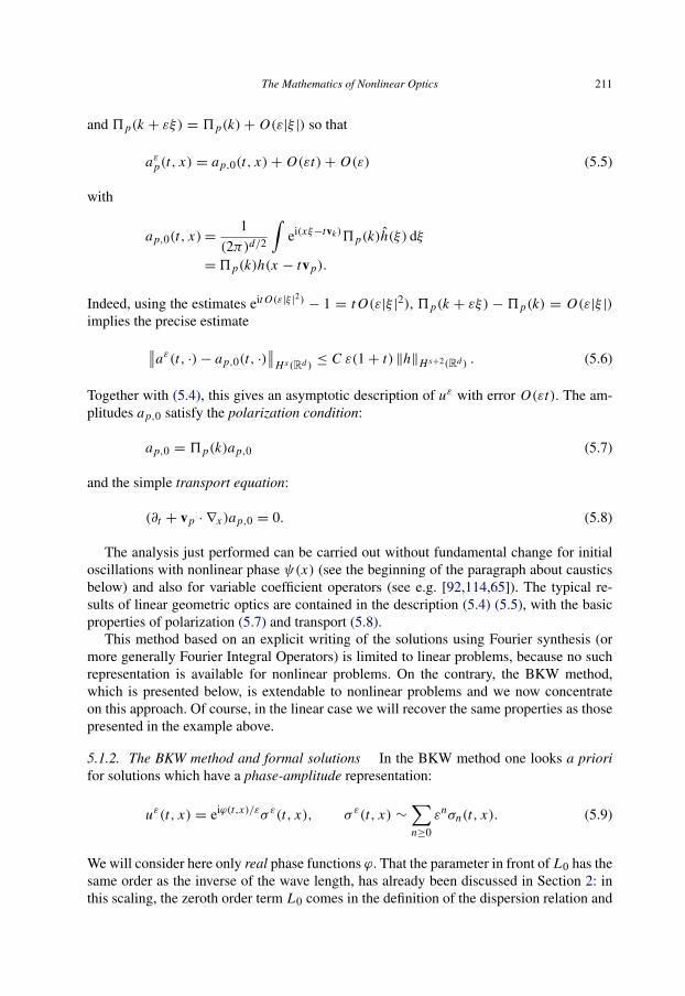
The Mathematics of Nonlinear Optics 211
and 5p(k + εξ) = 5p(k)+ O(ε|ξ |) so that
aεp(t, x) = ap,0(t, x)+ O(εt)+ O(ε) (5.5)
with
ap,0(t, x)=1
(2π)d/2
∫ei(xξ−tvk )5p(k)h(ξ) dξ
=5p(k)h(x − tvp).
Indeed, using the estimates eit O(ε|ξ |2)− 1 = t O(ε|ξ |2), 5p(k + εξ) −5p(k) = O(ε|ξ |)
implies the precise estimate∥∥aε(t, ·)− ap,0(t, ·)∥∥
H s (Rd )≤ C ε(1+ t) ‖h‖H s+2(Rd ) . (5.6)
Together with (5.4), this gives an asymptotic description of uε with error O(εt). The am-plitudes ap,0 satisfy the polarization condition:
ap,0 = 5p(k)ap,0 (5.7)
and the simple transport equation:
(∂t + vp · ∇x )ap,0 = 0. (5.8)
The analysis just performed can be carried out without fundamental change for initialoscillations with nonlinear phase ψ(x) (see the beginning of the paragraph about causticsbelow) and also for variable coefficient operators (see e.g. [92,114,65]). The typical re-sults of linear geometric optics are contained in the description (5.4) (5.5), with the basicproperties of polarization (5.7) and transport (5.8).
This method based on an explicit writing of the solutions using Fourier synthesis (ormore generally Fourier Integral Operators) is limited to linear problems, because no suchrepresentation is available for nonlinear problems. On the contrary, the BKW method,which is presented below, is extendable to nonlinear problems and we now concentrateon this approach. Of course, in the linear case we will recover the same properties as thosepresented in the example above.
5.1.2. The BKW method and formal solutions In the BKW method one looks a priorifor solutions which have a phase-amplitude representation:
uε(t, x) = eiϕ(t,x)/εσ ε(t, x), σ ε(t, x) ∼∑n≥0
εnσn(t, x). (5.9)
We will consider here only real phase functions ϕ. That the parameter in front of L0 has thesame order as the inverse of the wave length, has already been discussed in Section 2: inthis scaling, the zeroth order term L0 comes in the definition of the dispersion relation and

212 G. Metivier
in all the aspects of the propagation, as shown in the computations below. Examples arevarious versions of Maxwell’s equations coupled with the Lorentz model, or anharmonicoscillators, or with Bloch’s equations.
Introduce the symbol of the equation:
L(a, τ, ξ) = τ A0(a)+d∑
j=1
ξ j A j (a)− iE(a) = A0(a) (τ Id + G(a, ξ)) . (5.10)
Plugging the expansion (5.9) into the equation, and ordering in powers of ε, yields thefollowing cascade of equations:
L(a, dt,xϕ)σ0 = 0 (5.11)
iL(a, dt,xϕ)σn+1 + L1(a, ∂)σn = 0, n ≥ 0 (5.12)
with L1(a, ∂) = A0∂t +∑
A j∂x j .
DEFINITION 5.2. A formal solution is a formal series (5.9) which satisfies the equation inthe sense of formal series, that is, it satisfies the equations (5.11) and (5.12) for all n.
5.1.3. The dispersion relation and phases The first Eq. (5.11) has a nontrivial solutionσ0 6= 0 if and only if
– ϕ solves the eikonal equation
det (L (a(t, x), dϕ(t, x))) = 0 (5.13)
– σ0 satisfies the polarization condition
σ0(t, x) ∈ ker (L (a(t, x), dϕ(t, x))) . (5.14)
DEFINITIONS 5.3. (i) The equation det L(a, τ, ξ) = 0 is called the dispersion rela-tion. We denote by C the set of its solutions (a, τ, ξ).
(ii) A point (a, τ , ξ) ∈ C is called regular if, on a neighborhood of this point, C isgiven by an equation τ + λ(a, ξ) = 0, where λ is a smooth function near (a, ξ).We denote by Creg the manifold of regular points.
(iii) Given a Ck function a(t, x), k ≥ 2, ϕ is called a characteristic phase if is satisfiesthe eikonal equation (5.13).
(iv) A characteristic phase is said to be of constant multiplicity m if the dimension ofker L (a(t, x), dϕ(t, x)) is equal to m for all points (t, x).
(v) A characteristic phase is said to be regular if (a(t, x), dϕ(t, x)) ∈ Creg for all (t, x).
REMARKS 5.4. (1) A point (a, τ, ξ) belongs to C if and only if −τ is an eigenvalue ofG(a, ξ).

The Mathematics of Nonlinear Optics 213
(2) Because of the symmetry Assumption 5.1, G(a, ξ) has only real and semi-simpleeigenvalues and the dispersion relation has real coefficients. In particular the kernel andimage of τ Id + G(a, ξ) satisfy:
ker(τ Id + G(a, ξ)) ∩ im(τ Id + G(a, ξ)) = {0}. (5.15)
(3) If (a, τ , ξ) ∈ Creg , then for (a, ξ) in a neighborhood of (a, ξ), λ(a, ξ) is the onlyeigenvalue of G(a, ξ) close to −τ , proving that λ(a, ξ) has constant multiplicity. In partic-ular, a regular phase has constant multiplicity.
(4) If ϕ is a characteristic phase of constant multiplicity, then the kernelker L (a(t, x), dϕ(t, x)) and the image imL (a(t, x), dϕ(t, x)) are vector bundles of con-stant dimension, as smooth as dϕ with respect to (t, x).
EXAMPLES 5.5. (1) (Planar phases) If L has constant coefficients, for instance if a = ais fixed, then any solution of the dispersion relation, that is any eigenvalue −τ of G(a, ξ),yields a phase
ϕ(t, x) = τ t + ξ · x . (5.16)
This phase has constant multiplicity since L(a, dϕ
)is independent of (t, x).
(2) (Regular phases) If C = {τ + λ(a, ξ) = 0} near a regular point, then one can solve,locally, the Hamilton–Jacobi equation
∂tϕ + λ(a(t, x), ∂yϕ) = 0 (5.17)
using the method of characteristics (see e.g. [43,65]). The graph of dϕ is a union of integralcurves, called bi-characteristic curves, of the Hamiltonian field
H = ∂t +
d∑j=1
∂ξ jλ(a(t, x), ξ)∂x j −
d∑k=0
∂xkλ(a(t, x), ξ)∂ξk . (5.18)
Starting from an initial phase, ϕ0(x), one determines the initial manifold 30 =
{0, x,−λ(0, x, dxϕ0(x), dxϕ0(x))},and next, the manifold 3 which is the union of the bi-characteristic curves launched from 30. As long as the projection (t, x, τ, ξ) 7→ (t, x)from 3 to R1+d remains invertible, 3 is the graph of the differential of a function ϕ, thatis 3 = {(t, x, ∂tϕ, ∂xϕ)}, and ϕ is a solution of (5.17).
The projections on the (t, x) space of the bi-characteristic curves drawn in 3 are calledthe rays. They are integral curves of the field
X = ∂t +
d∑j=1
∂ξ jλ(a(t, x), dxϕ(t, x))∂x j . (5.19)
5.1.4. The propagator of amplitudes The Eq. (5.12) for n = 1 reads
iL(a, dt,xϕ)σ1 + L1(a, ∂)σ0 = 0.

214 G. Metivier
A necessary and sufficient condition for the existence of solutions is that L1(a, ∂)σ0 be-longs to the range of L(a, dϕ). Therefore, σ0 must satisfy:
σ0 ∈ ker L(a, dϕ), L1(a, ∂)σ0 ∈ imL(a, dϕ). (5.20)
Suppose that a is smooth and ϕ is a smooth characteristic phase of constant multiplicitym. In this case N (t, x) = ker L(a(t, x), dϕ(t, x)) and I(t, x) = imL(a(t, x), dϕ(t, x))define smooth vector bundles N and I with fiber of dimension m and N −m respectively.Introduce the quotient bundle N ′ := CN/I and the natural projection π : CN
7→ CN/I .The profile equations (5.20) read
σ0 ∈ C∞N , Lϕσ0 = 0 (5.21)
where C∞N denotes the C∞ sections of the bundle N and
Lϕ = πL1(a, ∂) (5.22)
is a first order system from C∞N to C∞N ′ . We will prove below that the Cauchy problem for(5.21) is well-posed and thus determines σ0. The operator Lϕ , acting from sections of Nto sections of N ′, is the intrinsic formulation of the propagation operator.
In order to make computations and proofs, it is convenient to use more practical formsof Lϕ . We give two of them.• Formulation using projectors. We still assume that ϕ is a smooth characteristic
phase of constant multiplicity m. Thus, there are smooth projectors P(t, x) and Q(t, x)on ker L(a(t, x), dϕ(t, x)) and imL(a(t, x), dϕ(t, x)), respectively, (see Remarks 5.4 4).They satisfy at each point (t, x):
(I − Q)L(a, dϕ) = 0, L(a, dϕ)P = 0. (5.23)
With these notations, the conditions (5.20) are equivalent to
σ0(t, x) = P(t, x)σ0(t, x), (5.24)
(I − Q)L1(a, ∂)σ0 = 0. (5.25)
In this setup, the transport operator reads
Lϕσ := (I − Q)L1(a, ∂)(Pσ) = A0,ϕ∂t +
d∑j=1
A j,ϕ∂x j + Eϕ (5.26)
where A j,ϕ = (Id − Q)A j P and Eϕ = (I − Q)L1(a, ∂)(P).
REMARK 5.6 (About the choice of projectors). The choice of the projectors P and Qis completely free. This does not mean a lack of uniqueness in the determination ofσ0 since all the formulations are equivalent to (5.20). Moreover, if P ′ and Q′ are other

The Mathematics of Nonlinear Optics 215
projectors on ker L and imL, respectively, there are matrices α and β such that P ′ = Pαand (Id − Q′) = β(Id − Q), since P and P ′ have the same image and (Id − Q) and(Id − Q′) have the same kernel. Therefore the operators L ′ϕ = (Id − Q′)A j P ′ and Lϕ areobviously conjugated and thus share the same properties.
Of course, the symmetry assumption suggests a natural choice: one can take P(t, x) tobe the spectral projector on ker(∂tϕ + G(a, dxϕ)), that is the projector on the kernel alongthe image of ∂tϕ+G(a, dxϕ). By the symmetry assumption, it is an orthogonal pojector forthe scalar product induced by A0(a(t, x)) so that A0 P = P∗A0, and the natural associatedprojector on the image is Q = A0(Id − P)A−1
0 = Id − P∗. This choice is natural andsufficient for a mathematical analysis and the reader can assume that this choice is madeall along theses notes.
• Formulation using parametrization of the bundles. Alternately, one can parametrize(at least locally) the kernel as
ker L(a(t, x), dϕ(t, x)) = ρ(t, x)Rm (5.27)
where ρ(t, x) is a smooth and injective N×m matrix. For instance, in the case of Maxwell’sequations, the kernel can be paramametrized by the E component (see Example 5.11 be-low). Similarly, one can parametrize the co-kernel of L(a, dϕ) and introduce a smoothm × N matrix ` of rank m such that
`(t, x)imL(a(t, x), dϕ(t, x)) = {0}. (5.28)
With these notations, the conditions (5.20) are equivalent to
σ0 = ρσ[, (5.29)
`L1(a, ∂)ρσ[= 0. (5.30)
For instance, L(a, dϕ) being self-adjoint, one can choose ` = ρ∗. In this setup, the trans-port operator reads
L[σ [ := `L1(a, ∂)(ρσ[) = A[0∂t +
d∑j=1
A[j∂x j + E[ (5.31)
where A[j = `A jρ and E[ = `L1(a, ∂)(ρ). It is clear that changing ρ [resp. `] is just alinear change of unknowns [resp. change of variables in the target space].
For instance, let (r1, . . . , rm) be a smooth basis of ker L(a, dϕ) (the columns of thematrix ρ) and let (`1, . . . , `m) be a smooth dual basis of left null vectors of L(a, dϕ) (therows of `). They can be normalized so that
`p(t, x)A0(a(t, x)rq(t, x)) = δp,q , 1 ≤ p, q ≤ m. (5.32)

216 G. Metivier
(One can choose the {rp} forming an orthonormal basis for the Hermitian scalar productinduced by A0 and thus `p = r∗p). The polarization condition (5.29) reads
σ(t, x) =m∑
p=1
σp(t, x)rp(t, x), (5.33)
with scalar functions σp. The equation (5.30) is
∂tσp(t, x)+d∑
j=1
m∑q=1
`p(t, x)∂x j
(A j (a(t, x))σq(t, x)rq(t, x)
)= `p f. (5.34)
With Eσ denoting the column m-vector with entries σp, the operator in the left-hand sidereads
L[ Eσ := ∂t Eσ +
d∑j=1
A[j∂x j Eσ + E[ Eσ (5.35)
where A[j is the m × m matrix with entries `p A jrq .
LEMMA 5.7 (Hyperbolicity of the propagation operator). Suppose that ϕ is a smoothcharacteristic phase of constant multiplicity. Then the first order system Lϕ on the smoothfiber bundle N = ker L(a, dϕ) is symmetric hyperbolic, in the sense that
(i) for any choice of projectors P and Q as above, there is a smooth matrix Sϕ(t, x)such that the matrices Sϕ A j,ϕ occurring in (5.26) are self-adjoint and Sϕ A0,ϕ ispositive definite on N ,or equivalently,
(ii) for any choice of matrices ρ and `, the m × m system L[ (5.31) is symmetric hy-perbolic.
PROOF. Using the Remark 5.6 it is sufficient to make the proof when P is the spectralprojector and (Id − Q) = P∗, in which case the result is immediate with S = Id .
For a general direct proof, note that f ∈ ker(Id − Q) when f ∈ imL(a, dϕ).Because of symmetry, imL(a, dϕ) = ker L(a, dϕ)⊥. Therefore, this space is equal to(imP)⊥ = ker P∗. This shows that ker(Id − Q) = ker P∗, implying that there is a smoothmatrix S such that
S(Id − Q) = P∗.
Therefore S A j,ϕ = P∗A j P is symmetric and S A0,ϕP = P∗A0 P is positive definite on N .The proof for the L[ representation is quite similar. �
The classical existence theory for symmetric hyperbolic systems can be transported tovector bundles, for instance using the existence theory for L[. It can also be localized on
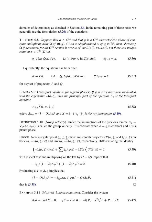
The Mathematics of Nonlinear Optics 217
domains of determinacy as sketched in Section 3.6. In the remaining part of these notes wegenerally use the formulation (5.26) of the equations.
THEOREM 5.8. Suppose that a ∈ C∞ and that ϕ is a C∞ characteristic phase of con-stant multiplicity near � of (0, x). Given a neighborhood ω of x in Rd , then, shrinking� if necessary, for all C∞ section h over ω of ker L(a(0, x), dϕ(0, x)) there is a uniquesolution σ ∈ C∞(�) of
σ ∈ ker L(a, dϕ), L1(a, ∂)σ ∈ imL(a, dϕ), σ|t=0 = h. (5.36)
Equivalently, the equations can be written
σ = Pσ, (Id − Q)L1(a, ∂)Pσ = 0, Pσ|t=0 = h (5.37)
for any set of projectors P and Q.
LEMMA 5.9 (Transport equations for regular phases). If ϕ is a regular phase associatedwith the eigenvalue λ(a, ξ), then the principal part of the operator Lϕ is the transportoperator
A0,ϕX (t, x, ∂t,x ) (5.38)
where A0,ϕ = (I − Q)A0 P and X = ∂t + vg · ∂x is the ray propagator (5.19).
DEFINITION 5.10 (Group velocity). Under the assumptions of the previous lemma, vg =
∇ξλ(a, ∂xϕ) is called the group velocity. It is constant when a = a is constant and a is aplanar phase.
PROOF. Near a regular point (a, τ , ξ) there are smooth projectors P(a, ξ) and Q(a, ξ) onker L(a,−λ(a, ξ), ξ) and imL(a,−λ(a, ξ), ξ), respectively. Differentiating the identity(
−λ(a, ξ)A0(a)+∑
ξ j A j (a)− iE(a))
P(a, ξ) = 0 (5.39)
with respect to ξ and multiplying on the left by (I −Q) implies that
−∂ξ jλ(I −Q)A0 P + (I −Q)A j P = 0. (5.40)
Evaluating at ξ = dxϕ implies that
(I − Q)A j P = −∂ξ jλ(a, dxϕ)(I − Q)A0 P, (5.41)
that is (5.38). �
EXAMPLE 5.11 (Maxwell–Lorentz equations). Consider the system
∂t B + curl E = 0, ∂t E − curl B = −∂t P, ε2∂2t P + P = γ E (5.42)
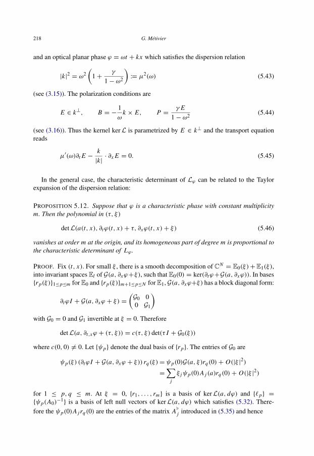
218 G. Metivier
and an optical planar phase ϕ = ωt + kx which satisfies the dispersion relation
|k|2 = ω2(
1+γ
1− ω2
):= µ2(ω) (5.43)
(see (3.15)). The polarization conditions are
E ∈ k⊥, B = −1ω
k × E, P =γ E
1− ω2 (5.44)
(see (3.16)). Thus the kernel ker L is parametrized by E ∈ k⊥ and the transport equationreads
µ′(ω)∂t E −k
|k|· ∂x E = 0. (5.45)
In the general case, the characteristic determinant of Lϕ can be related to the Taylorexpansion of the dispersion relation:
PROPOSITION 5.12. Suppose that ϕ is a characteristic phase with constant multiplicitym. Then the polynomial in (τ, ξ)
det L(a(t, x), ∂tϕ(t, x)+ τ, ∂xϕ(t, x)+ ξ) (5.46)
vanishes at order m at the origin, and its homogeneous part of degree m is proportional tothe characteristic determinant of Lϕ .
PROOF. Fix (t, x). For small ξ , there is a smooth decomposition of CN= E0(ξ)+E1(ξ),
into invariant spaces El of G(a, ∂xϕ+ξ), such that E0(0) = ker(∂tϕ+G(a, ∂xϕ)). In bases{rp(ξ)}1≤p≤m for E0 and {rp(ξ)}m+1≤p≤N for E1, G(a, ∂xϕ+ξ) has a block diagonal form:
∂tϕ I + G(a, ∂xϕ + ξ) =
(G0 00 G1
)with G0 = 0 and G1 invertible at ξ = 0. Therefore
det L(a, ∂t,xϕ + (τ, ξ)) = c(τ, ξ) det(τ I + G0(ξ))
where c(0, 0) 6= 0. Let {ψp} denote the dual basis of {rp}. The entries of G0 are
ψp(ξ) (∂tϕ I + G(a, ∂xϕ + ξ)) rq(ξ)=ψp(0)G(a, ξ)rq(0)+ O(|ξ |2)
=
∑j
ξ jψp(0)A j (a)rq(0)+ O(|ξ |2)
for 1 ≤ p, q ≤ m. At ξ = 0, {r1, . . . , rm} is a basis of ker L(a, dϕ) and {`p} =
{ψp(A0)−1} is a basis of left null vectors of ker L(a, dϕ) which satisfies (5.32). There-
fore the ψp(0)A jrq(0) are the entries of the matrix A[j introduced in (5.35) and hence

The Mathematics of Nonlinear Optics 219
det(τ I + G0(ξ)) = det(τ I +
∑ξ j A[j
)+ O
((|τ | + |ξ |)m+1
).
The proposition follows. �
REMARK 5.13. When the phase is regular of multiplicity m, Lemma 5.9 asserts that thefirst order part of the propagator is L[ = X I , whose characteristic determinant is
det L[(τ, ξ) =(τ +
∑ξ j∂ξ jλ(a, ∂xϕ)
)m.
Therefore, we recover that
det L(a, ∂t,xϕ + (τ, ξ))= c(τ, ξ) (τ + ∂tϕ + λ(a, ∂xϕ + ξ))m
= c det L[(τ, ξ)+ O((|τ | + |ξ |)m+1
).
From a geometrical point of view, this means that the characteristic manifold of L[ is thetangent space of Creg at (a, dϕ). In general, the geometrical meaning of Proposition 5.12is that the characteristic manifold of L[ is the tangent cone of C at (a, dϕ).
EXAMPLE 5.14 (Conical refraction). Consider Maxwell’s equations in a bi-axial crystal.With notations as in see (3.19), the characteristic determinant satisfies
det L(τ, ξ) =14τ 2((2τ 2
−9)2 − (P2+ Q2)).
There are exceptional points in the characteristic variety C which are not regular: this hap-pens when P2
+Q = 0 and τ = ± 129, whose explicit solution is given in (3.20). Consider
such a point (ω, k) ∈ C \ Creg and the planar phase ϕ = ωt + kx , which has constant mul-tiplicity m = 2, see Examples 5.5 (1). Near this point,
det L(∂t,xϕ + (τ, ξ))= c((4τ − ξ ·9 ′(k))2
− (ξ · P ′(k))2 − (ξ · Q′(k))2)+ h.o.t.
Thus the relation dispersion of Lϕ is(4τ − ξ ·9 ′(k)
)2− (ξ · P ′(k))2 − (ξ · Q′(k))2 = 0.
Because P ′(k) and Q′(k) are linearly independent, this cannot be factored and this is thedispersion relation of a wave equation, not of a transport equation. We refer the reader to[102,76], for instance, for more details.
5.1.5. Construction of WKB solutions
THEOREM 5.15 (WKB solutions). Suppose that a ∈ C∞ and that ϕ is a C∞ characteris-tic phase of constant multiplicity m on a neighborhood � of (0, x). Given a neighborhoodω of x, shrinking � is necessary, for all sequence of functions hn ∈ C∞(ω) satisfying
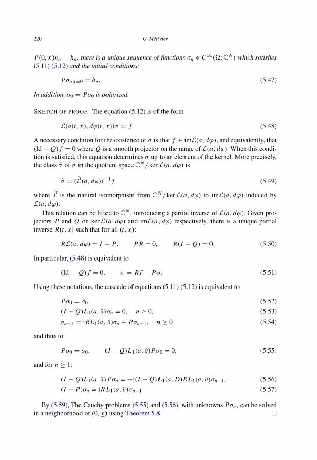
220 G. Metivier
P(0, x)hn = hn , there is a unique sequence of functions σn ∈ C∞(�;CN ) which satisfies(5.11) (5.12) and the initial conditions:
Pσn |t=0 = hn . (5.47)
In addition, σ0 = Pσ0 is polarized.
SKETCH OF PROOF. The equation (5.12) is of the form
L(a(t, x), dϕ(t, x))σ = f. (5.48)
A necessary condition for the existence of σ is that f ∈ imL(a, dϕ), and equivalently, that(Id − Q) f = 0 where Q is a smooth projector on the range of L(a, dϕ). When this condi-tion is satisfied, this equation determines σ up to an element of the kernel. More precisely,the class σ of σ in the quotient space CN/ ker L(a, dϕ) is
σ = (L(a, dϕ))−1 f (5.49)
where L is the natural isomorphism from CN/ ker L(a, dϕ) to imL(a, dϕ) induced byL(a, dϕ).
This relation can be lifted to CN , introducing a partial inverse of L(a, dϕ). Given pro-jectors P and Q on ker L(a, dϕ) and imL(a, dϕ) respectively, there is a unique partialinverse R(t, x) such that for all (t, x):
RL(a, dϕ) = I − P, P R = 0, R(I − Q) = 0. (5.50)
In particular, (5.48) is equivalent to
(Id − Q) f = 0, σ = R f + Pσ. (5.51)
Using these notations, the cascade of equations (5.11) (5.12) is equivalent to
Pσ0 = σ0, (5.52)
(I − Q)L1(a, ∂)σn = 0, n ≥ 0, (5.53)
σn+1 = iRL1(a, ∂)σn + Pσn+1, n ≥ 0 (5.54)
and thus to
Pσ0 = σ0, (I − Q)L1(a, ∂)Pσ0 = 0, (5.55)
and for n ≥ 1:
(I − Q)L1(a, ∂)Pσn = −i(I − Q)L1(a, D)RL1(a, ∂)σn−1, (5.56)
(I − P)σn = iRL1(a, ∂)σn−1. (5.57)
By (5.59), The Cauchy problems (5.55) and (5.56), with unknowns Pσn , can be solvedin a neighborhood of (0, x) using Theorem 5.8. �

The Mathematics of Nonlinear Optics 221
The initial conditions (5.47) can be replaced by conditions of the form
Hσn |t=0 = hn (5.58)
where H is an m × N matrix, which depends smoothly on x , and such that
ker H(x) ∩ ker L(a(0, x), dϕ(0, x)) = {0}. (5.59)
THEOREM 5.16. Suppose that a ∈ C∞ and that ϕ is a C∞ characteristic phase of con-stant multiplicity m on a neighborhood � of (0, x). Given a neighborhood ω of x, shrink-ing � is necessary, for all sequences of functions hn ∈ C∞(ω;Cm), there is a uniquesequence of solutions σn ∈ C∞(�;CN ) of (5.11) (5.12) and the initial conditions (5.58).
Indeed, the nth initial condition reads
H Pσn |t=0 = hn − H(Id − P)σn |t=0 = hn − iH RL1σn−1|t=0.
Knowing σn−1, the assumption (5.59) implies that this equation can be solved and give thedesired initial conditions for Pσn |t=0.
REMARK 5.17 (About the choice of projectors). The projector P intervenes in the formu-lation of the Cauchy condition (5.47). We point out here that the coefficients σn do notdepend on splitting the (5.53) (5.54) equations, where one could use as well other projec-tors P ′ and Q′: the equations are always equivalent to (5.11) (5.12) and the theorem assertsuniqueness. Moreover, the set of asymptotic solutions obtained by this construction doesnot depend on the projector P used for the initial condition.
REMARK 5.18. Imposing initial conditions for the Pσn is natural from the proof. Wefollow this approach in the remaining part of these notes. However, in applications, theformulation (5.58) may be better adapted to physical considerations. For instance, whenconsidering Maxwell’s equations as in (5.42), it makes sense to impose initial conditionson the electric field, or on the electric induction (see Example 5.11).
5.1.6. Approximate solutions Given (σ0, . . . , σn) ∈ C∞ solutions of (5.11) (5.12) for0 ≤ k ≤ n, the family of functions
uεapp,n(t, x) =n∑
k=0
εkσk(t, x)eiϕ(t,x)/ε (5.60)
satisfies the Eq. (5.1) with an error term of order O(εn), that is
L(a, ∂)uεapp,n = εn fneiϕ/ε (5.61)
where fn = QL1(a, ∂)σn is smooth.

222 G. Metivier
If {σn}n∈N is a family of solutions of (5.11) (5.12), one can use Borel’s Theorem toconstruct asymptotic solutions
uεapp(t, x) = σ ε(t, x)eiϕ(t,x)/ε, σ ε(t, x) ∼∑k≥0
εkσk(t, x) (5.62)
where the symbol ∼ means that for all n and all m:
σ ε −∑k≤n
εkσk = O(εn+1) in Cm . (5.63)
In this case
L(a, ∂)uεapp = rεeiϕ/ε (5.64)
where rε = O(ε∞) in C∞, meaning that for all n and all m,
rε = O(εn) in Cm . (5.65)
Note that this also implies that
rεeiϕ/ε= O(ε∞) in C∞. (5.66)
5.1.7. Exact solutions The construction of exact solutions uε of L(a, ∂)uε = 0 close tothe approximate solutions uεapp amounts to solving the equation for the difference
L(a, ∂)(uε − uεapp) = −rεeiϕ/ε. (5.67)
Because this system is symmetric hyperbolic and linear, the Cauchy problem is locallywell-posed. The question is how to obtain estimates for the difference uε−uεapp, which areuniform in ε. The symmetry immediately implies uniform L2 estimates. The proof of uni-form Sobolev estimates is more delicate when the term ε−1 E(a) is present in the Eq. (5.1),as discussed in Section 4. In all cases, the method of weighted estimates using H s
ε normscan be applied. Combining Theorems 5.15 and 4.21, localized on domains of determinacyas in Section 3.6, implies the following.
THEOREM 5.19. Suppose that a ∈ C∞ and that ϕ is a C∞ characteristic phase of con-stant multiplicity near (0, x), and suppose that {hn}n∈N is a sequence of C∞ functions ona fixed neighborhood of x, such that P(0, x)hn(x) = hn(x). Then there are C∞ solutionsuε of L(a, ∂)uε = 0 in a neighborhood of (0, x), independent of ε, such that
uε = σ εeiϕ/ε, σ ε ∼∑n≥0
εnσn

The Mathematics of Nonlinear Optics 223
where the {σn}n∈N are the unique solutions of (5.11) (5.12) such that Pσn |t=0 = hn . Inparticular
Puε |t=0 = hεeiϕ(0, · )/ε, hε ∼∑n≥0
εnhn .
5.2. Weakly nonlinear geometric optics
To fix the notations, consider here the first order system
L(a, u, ∂)u :=
(εA0(a, u)∂t +
d∑j=1
εA j (a, u)∂x j + E(a)
)u
= f (a, u), (5.68)
where f is a smooth function with f (a, 0) = 0,∇u f (a, 0) = 0. The A j are smoothand symmetric matrices and E is skew symmetric. To model high frequency oscillatorynonlinear waves, one looks for solutions of the form
uε(t, x) ∼ ε p∑n≥0
εnUn(t, x, ϕ(t, x)/ε). (5.69)
There are two differences with (5.9):
– because of the nonlinearity, harmonics eikϕ/ε are expected, yielding to general peri-odic functions of ϕ/ε and thus profiles Un(t, x, θ) that are periodic in θ , see Section 7for an elementary example.
– a prefactor ε p, which measures the amplitude of the oscillations. When p is large, thewave is small and driven by the linear part L(a, 0, ∂), the nonlinear effects appear-ing only as perturbations of the principal term. Decreasing p, the weakly nonlinearregime is reached when the nonlinear effects are present in the propagation of theprincipal term U0.
For general quasi-linear equations (5.68) and quadratic nonlinearities, this correspondsto p = 1. When the nonlinearities are cubic, then the natural scaling is p = 1
2 (see thegeneral discussion in [41]). In the remaining part of this section, we mainly concentrate onthe most general case with p = 1 (see however the third example in Remarks 5.26).
Other regimes of strongly nonlinear geometric optics will be briefly discussed in thesubsequent sections.
REMARK 5.20 (Other frameworks). In the framework presented here, u0 = 0 is a solutionof (5.68) and we study perturbations of this particular solution. The analysis applies as wellto slightly different equations. For instance, one can replace the condition f = O(|u|2) byf = ε f and consider perturbations of nonconstant solutions. Examples are systems
L(u, ∂)u :=
(A0(u)∂t +
d∑j=1
A j (u)∂x j +1ε
E
)u = f (u). (5.70)

224 G. Metivier
Note that the prefactor ε p has to be adapted to this setting. We leave it to the reader to writedown the corresponding modifications. Some of the examples below concern this class ofequations.
5.2.1. Asymptotic equations With p = 1, plug the expansion (5.69) into the equation,expand in a power series of ε and equate to zero the coefficients. We obtain a cascade ofequations:
L0(a, dϕ, ∂θ )U0 = 0, (5.71)L0(a, dϕ, ∂θ )Un+1 + L1(a,U0, ∂t,x,θ )Un = Fn, n ≥ 0, (5.72)
where
L0(a, dϕ, ∂θ ) =
(d∑
j=0
∂ jϕA j (a, 0)
)∂θ + E(a),
L1(a, v, ∂t,x,θ ) = L1(a, 0, ∂t,x )+ B(a, dϕ, v)∂θ ,
with
L1(a, 0, ∂t,x ) =
d∑j=0
A j (a, 0)∂ j , B(a, dϕ, v) =d∑
j=0
∂ jϕ v · ∇u A j (a, 0).
Moreover,
F0 = ∇2 f (a, 0)(U0,U0),
Fn = 2∇2 f (a, 0)(U0,Un)−
d∑j=0
∂ jϕ Un · ∇u A j (a, 0)∂θU0 + Gn−1
where Gn−1 depends only on (U0, . . . ,Un−1).The operator L0 has constant coefficients in θ . Using Fourier series,
U (t, x, θ) =∑α∈Z
Uα(t, x)eiαθ , (5.73)
L0(a, dϕ, ∂θ )U =∑α
iL(a, αdϕ)Uα(t, x)eiαθ
where L(a, τ, ξ) is the symbol (5.10) associated with the operator L(a, 0, ∂). For L0 tohave a nontrivial kernel, at least one phase αϕ must be characteristic. Changing ϕ is neces-sary, we assume that this occurs for α = 1. Next, the analysis is quite different dependingon whether or not E = 0. In the former case, all the harmonics are characteristic; in thelatter, the harmonics are not expected to be characteristic in general, except α = −1 if oneconsiders real-valued solutions. The following assumptions are satisfied in virtually allcases of application. They give a convenient framework for the construction of asymptoticsolutions.
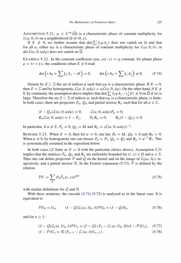
The Mathematics of Nonlinear Optics 225
ASSUMPTION 5.21. ϕ ∈ C∞(�) is a characteristic phase of constant multiplicity forL(a, 0, ∂) on a neighborhood � of (0, x).
If E 6= 0, we further assume that det(∑∂ jϕA j ) does not vanish on � and that
for all α, either αϕ is a characteristic phase of constant multiplicity for L(a, 0, ∂), ordet L(a, 0, αdϕ) does not vanish on �.
EXAMPLE 5.22. In the constant coefficient case, a(t, x) = a constant, for planar phaseϕ = τ t + ξ x , the conditions when E 6= 0 read
det(τ A0 +
∑ξ j A j − iE
)= 0, det
(τ A0 +
∑ξ j A j
)6= 0. (5.74)
Denote by Z ⊂ Z the set of indices α such that αϕ is a characteristic phase. If E = 0,then Z = Z and by homogeneity, L(a, 0, αdϕ) = αL(a, 0, dϕ). On the other hand, if E 6=0, by continuity, the assumption above implies that det(
∑∂ jϕA j−i 1
αE) 6= 0 on� if |α| is
large. Therefore the set Z ⊂ Z of indices α, such that αϕ is a characteristic phase, is finite.In both cases, there are projectors Pα , Qα and partial inverse Rα such that for all α ∈ Z.
(I − Qα)L(a, 0, αdϕ) = 0, L(a, 0, αdϕ)Pα = 0,
RαL(a, 0, αdϕ) = I − Pα, PαRα = 0, Rα(I − Qα) = 0.
In particular, if α 6∈ Z , Pα = 0, Qα = Id and Rα = (L(a, 0, αdϕ))−1.
REMARK 5.23. When E = 0, then for α = 0, one has P0 = Id , Q0 = 0 and R0 = 0.When α 6= 0, by homogeneity one can choose Pα = P1, Qα = Q1 and Rα = α−1 R1. Thisis systematically assumed in the exposition below.
In both cases (Z finite or E = 0 with the particular choice above), Assumption 5.21implies that the matrices Pα , Qα and Rα are uniformly bounded for (t, x) ∈ � and α ∈ Z.Thus one can define projectors P and Q on the kernel and on the image of L0(a, ∂θ ), re-spectively, and a partial inverse R. In the Fourier expansion (5.73), P is defined by therelation
P U =∑α
PαUα(t, x)eiαθ (5.75)
with similar definitions for Q and R.With these notations, the cascade (5.71) (5.72) is analyzed as in the linear case. It is
equivalent to
P U0 = U0, (I −Q)L1(a,U0, ∂)P U0 = (I −Q)F0, (5.76)
and for n ≥ 1:
(I −Q)L1(a,U0, ∂)P Un = (I −Q) (Fn − L1(a,U0, D)(I − P)Un) , (5.77)
(I − P)Un = R (Fn−1 − L1(a, ∂)Un−1) . (5.78)

226 G. Metivier
REMARK 5.24. As in Remark 5.6, the choice of projectors Pα , Qα is free. The naturalchoice is to take spectral projectors, that is Pα(t, x) orthogonal with respect to its scalarproduct defined by A0(a(t, x)) and Qα = A0(Id − Pα)A
−10 = Id − P∗α .
5.2.2. The structure of the profile equations I: the dispersive case We consider here thecase where E 6= 0. In this case the set Z of characteristic harmonics is finite, and thepolarization condition in (5.76) reads
U0(t, x, θ) =∑α∈Z
U0,α(t, x)eiαθ , PαU0,α = U0,α (5.79)
and the equation is a coupled system for the {U0,α}α∈Z :
(I − Qα)L1(a, 0, ∂)PαU0,α = (I − Qα)∑
β+γ=α
0α,β,γ
(U0,β , U0,γ
)(5.80)
with
0α,β,γ (U, V ) = −iγ B(a, dϕ,U )V +∇2 f (a)(U, V ). (5.81)
The linear analysis applies to the left-hand side in (5.80). It is hyperbolic and is a transportequation if αϕ is a regular phase, as explained in Lemmas 5.7 and 5.9. Choosing bases inthe ranges of the Pα , it can be made explicit as in (5.34). In general, the quadratic termin the right-hand side of (5.80) does not vanish, so that the system for U0 appears as asemi-linear hyperbolic system.
EXAMPLE 5.25 (Maxwell – anharmonic Lorentz equations). Consider the system
∂t B + curl E = 0, ∂t E − curl B = −∂t P,
ε2∂2t P + P + V (P) = γ E (5.82)
where V is at least quadratic. We apply the general computations above, that is,to asymptotic expansions of order O(ε). The dispersion relation is the same as forMaxwell–Lorentz. Consider an optical planar phase ϕ = ωt + kx which satisfies the dis-persion relation
|k|2 = ω2(
1+γ
1− ω2
):= µ2(ω). (5.83)
The set of the harmonics which satisfies the dispersion relations is Z = {−1, 0,+1}. Thepolarization conditions for harmonic +1 and −1 are
E±1 ∈ k⊥, B±1 = −1ω
k × E±1, P±1 =γ E±1
1− ω2 . (5.84)

The Mathematics of Nonlinear Optics 227
Physical solutions correspond to real valued fields, that is, they satisfy the conditions
E−1 = E1. The polarization conditions for the harmonic 0 (the mean field) reduce to
P0 = γ E0. (5.85)
The profile equations readµ′(ω)∂t E1 −k
|k|· ∂x E1 = i
γω2
2|k|(1− ω2)(V2(E0, E1))⊥,
∂t B0 + curl E0 = 0, (1+ γ )∂t E0 − curl B0 = 0(5.86)
where V2 is the quadratic part of V at the origin and A⊥ is the projection of A on k⊥.
REMARKS 5.26. (1) (Rectification). When only the harmonics −1, 0,+1 are present,one expects from equation (5.80) a quadratic coupling of U1 and U−1 as a sourceterm for the propagation of U0, implying that a mean field U0 can be created byoscillatory waves. This phenomenon is called optical rectification. It is not presentin the case of (5.86) where, in addition, the propagation equation for U0 is linear.Rectification occurs in optics, but for different equations.
(2) (Generation of harmonics). For non-isotropic crystals (see (2.18), (2.19)), the dis-persion relation is non-isotropic in k, and for special values of k the harmonic(2ω, 2k) can be characteristic, see [39]. In this case, the analogue of (5.86) couplesE1 and E2. This nonlinear phenomenon is used in physical devices for doublingfrequencies.
EXAMPLE 5.27 (Generic equations for cubic nonlinearities). When V is cubic, the sys-tem (5.86) is linear. In this case, the regime of weakly nonlinear optics is not reached for
amplitudes O(ε), but for amplitudes O(ε12 ). All the computations can be carried out with
the prefactor√ε in front of the sum in (5.69) in place of ε (see [39,41]). For instance,
consider the cubic model (2.21) with no damping and oscillations with amplitudes of order
ε12 . With mean field E0 = 0, the transport equations for E1 are of the form:
∂t E1 + vg∂x E1 = iδ(|E1|
2 E1 +12(E1 · E1)E1
). (5.87)
The solutions of this system can be computed explicitly using the conservations
(∂t + vg∂x )|E1|2= 0, (∂t + vg∂x )(E1 × E1) = 0.
The solutions are determined from their initial data E1|t=0 = A ∈ k⊥:
E1(t, x) = eit I (x−vg t)R(tφ(x − vgt)) A(x − vgt)
where R(s) is the rotation of angle s in the plane k⊥, oriented by the direction of k and

228 G. Metivier
I =3δ2| A|2, φ =
iδ2|k|
k · (A × A).
Two physical nonlinear phenomena are described by this formula:
• the polarization of the electric field rotates at the speed φ in the plane k⊥;• when incorporated in the phase (ωt + kx)/ε, the term t I corresponds to a self-
modulation of the phase, depending on the intensity of the field.
5.2.3. The structure of the profile equation II: the non-dispersive case; the genericBurger’s equation We now assume that E = 0. In this case the set of characteristicfrequencies is Z = Z. By homogeneity, there are only two different possibilities:{
α = 0 : P0 = Id , Q0 = 0, R0 = 0,α 6= 0 : Pα = P1, Qα = Q1, Rα = R1.
It is convenient to split a periodic function U (θ) into its mean value U = MU = U0 andits oscillating part U∗ = OsU = U −U . Dropping several subscripts 1 in P1 etc, the Eq.(5.76) readsPU∗0 = U∗0 ,
(I − Q)L1(a, 0, ∂)PU∗0 = (I − Q)Os (0(U0,U0)) ,
L1(a, 0, ∂)U 0 =M (0(U0,U0))
with
0(U, V ) = ∇2 f (a)(U0,U0)− B(a, dϕ,U )∂θV .
REMARKS 5.28. (1) The case of conservation laws. For balance laws (3.2), the matricesA j (u) are the Jacobian matrices ∇ f j (u) of the fluxes f j . Thus
B(dϕ,U )∂θU =12∂θ
(∑∂ jϕ∇
2u f j (0)(U,U )
):=
12∂θ (b(dϕ)(U,U )) (5.88)
implying that
M (B(dϕ,U )∂θU ) = 0.
For conservation laws, the source term f vanishes and the equation for U 0 decouples andreduces to the linearized equation L1(0, ∂t,x )U 0 = 0. In particular, U 0 = 0 if its initialvalue vanishes and the equation for U∗0 reduces to{
PU∗0 = U∗0 ,
(I − Q)L1(a, 0, ∂)PU∗0 +12(I − Q)∂θ
(b(dϕ)(U∗0 ,U
∗
0 ))= 0.
(5.89)

The Mathematics of Nonlinear Optics 229
PROPOSITION 5.29 (Self-interaction coefficient for simple modes). Suppose that
(a) λ(a, u, ξ) is a simple eigenvalue of A−10 (a, u)
∑ξ j A j (a, u) for (a, u, ξ) close to
(a, 0, ξ), with eigenvector R(a, u, ξ) normalized by the condition t R A0 R = 1(which means that R is unitary for the scalar product defined by A0);
(b) the phase ϕ is a a solution of the eikonal equation
∂tϕ + λ(a(t, x), 0, ∂xϕ) = 0 (5.90)
for (t, x) close to (0, x), with ∂xϕ(0, x) = ξ .
Then,
(i) the polarization condition PU∗0 = U∗0 reads
U∗0 (t, x, θ) = σ(t, x, θ)r(t, x),
r(t, x) = R(a(t, x), 0, ∂xϕ(t, x)),(5.91)
(ii) the equation for σ deduced from the equation for U∗0 reads
∂tσ + vg · ∂xσ + b0(U 0)∂θσ + γ ∂θσ2= Os F(U 0, σ ) (5.92)
where vg = ∂ξλ(a, 0, ∂xϕ) is the group velocity as in (5.19), the self-interaction coefficientγ is
γ =12
r · ∇uλ(a, 0, ∂xϕ). (5.93)
The term b0 is linear in U 0 and F is at most quadratic.In particular, for systems of balance laws, b0 = 0. For systems of conservation laws
and a = a constant, with a planar phase ϕ = ωt + ξ · x, the equation reduces to
∂tσ + vg · ∂xσ + γ ∂θσ2= 0. (5.94)
The coefficient γ vanishes exactly when the eigenvalue λ(a, ·, ξ) is linearly degenerate atu = 0.
PROOF. We proceed as in Remark 5.6, noticing, that by symmetry, the right kernel of−λA0 +
∑ξ j A j is generated by t R. The equation is therefore
tr L1(a, 0, ∂t,x )(σr) = Ostr0(U 0 + σr,U 0 + σr).
The left-hand side is (∂t+vg ·∂x )σ+cσ , as explained in Lemma 5.9. Similarly, differentiat-ing in u the identity (−λA0+
∑ξ j A j )r = 0, and multiplying on the left by tr implies that
tr B(a, dϕ, v) = v · ∇uλ(a, 0, ∂xϕ)tr A0.
This implies the proposition. �
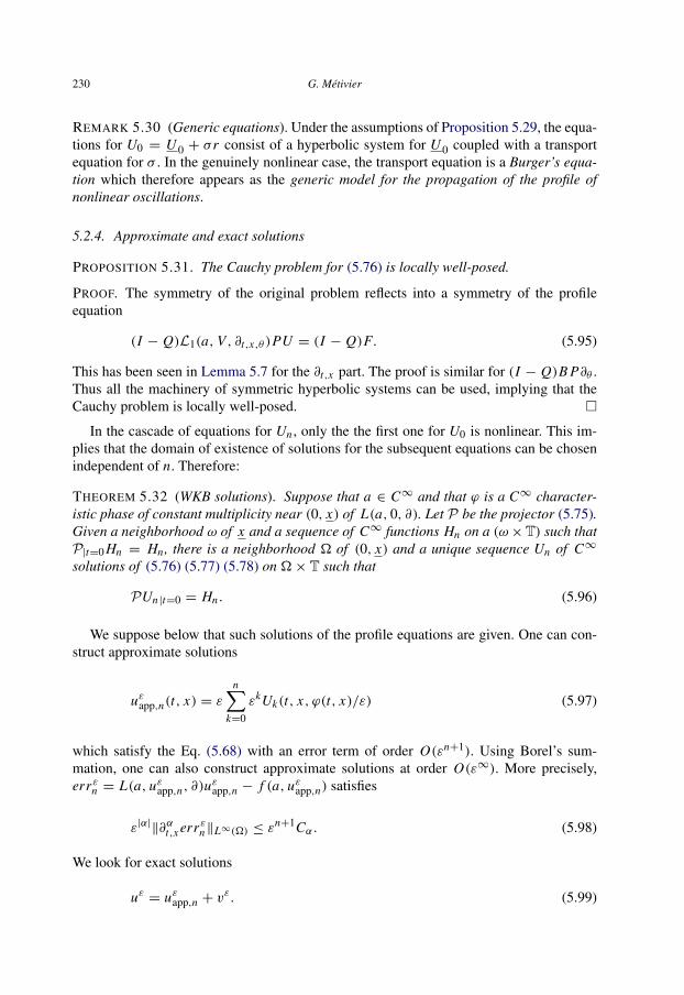
230 G. Metivier
REMARK 5.30 (Generic equations). Under the assumptions of Proposition 5.29, the equa-tions for U0 = U 0 + σr consist of a hyperbolic system for U 0 coupled with a transportequation for σ . In the genuinely nonlinear case, the transport equation is a Burger’s equa-tion which therefore appears as the generic model for the propagation of the profile ofnonlinear oscillations.
5.2.4. Approximate and exact solutions
PROPOSITION 5.31. The Cauchy problem for (5.76) is locally well-posed.
PROOF. The symmetry of the original problem reflects into a symmetry of the profileequation
(I − Q)L1(a, V, ∂t,x,θ )PU = (I − Q)F. (5.95)
This has been seen in Lemma 5.7 for the ∂t,x part. The proof is similar for (I − Q)B P∂θ .Thus all the machinery of symmetric hyperbolic systems can be used, implying that theCauchy problem is locally well-posed. �
In the cascade of equations for Un , only the the first one for U0 is nonlinear. This im-plies that the domain of existence of solutions for the subsequent equations can be chosenindependent of n. Therefore:
THEOREM 5.32 (WKB solutions). Suppose that a ∈ C∞ and that ϕ is a C∞ character-istic phase of constant multiplicity near (0, x) of L(a, 0, ∂). Let P be the projector (5.75).Given a neighborhood ω of x and a sequence of C∞ functions Hn on a (ω×T) such thatP|t=0 Hn = Hn , there is a neighborhood � of (0, x) and a unique sequence Un of C∞
solutions of (5.76) (5.77) (5.78) on �× T such that
P Un |t=0 = Hn . (5.96)
We suppose below that such solutions of the profile equations are given. One can con-struct approximate solutions
uεapp,n(t, x) = εn∑
k=0
εkUk(t, x, ϕ(t, x)/ε) (5.97)
which satisfy the Eq. (5.68) with an error term of order O(εn+1). Using Borel’s sum-mation, one can also construct approximate solutions at order O(ε∞). More precisely,errεn = L(a, uεapp,n, ∂)u
εapp,n − f (a, uεapp,n) satisfies
ε|α|‖∂αt,x errεn‖L∞(�) ≤ εn+1Cα. (5.98)
We look for exact solutions
uε = uεapp,n + vε. (5.99)

The Mathematics of Nonlinear Optics 231
The equation for vε has the form (4.49):
A0(b, v)∂tv +
d∑j=1
A j (b, v)∂x j v +1ε
E(a)v = F(b, v) (5.100)
where b = (a, uεapp,n) is uniformly bounded and satisfies estimates (4.50) for α > 0:
ε|α|−1‖∂αt,x b‖L∞(�) ≤ Cα. (5.101)
The derivatives of F(b, 0) = ε−1errεn are controlled by (5.98). Moreover, A j (b, v) =A j (a, uεapp,n + v). Therefore, we are in a position to apply Theorem 4.21, localized on asuitable domain of determinacy, shrinking � if necessary. Consider initial data hε whichsatisfy for |α| ≤ s
ε|α|‖∂αx h‖L2(ω) ≤ εnCα. (5.102)
THEOREM 5.33. If n > 1+ d/2, there are ε1 > 0 and a neighborhood � of (0, x), suchthat for ε ∈ ]0, ε1], the Cauchy problem for (5.68) with initial data uεapp,n |t=0 + hε, has a
unique solution uε ∈ C0 H s(�) for all s, and which satisfies
ε|α|‖∂αx (uε(t)− uεapp,n(t))‖L2 ≤ ε
nCα. (5.103)
In particular, this implies that
‖∂αx (uε(t)− uεapp,n(t))‖L∞ ≤ ε
n− d2−|α|Cα. (5.104)
REMARK 5.34 (About domains of determinacy). All the analysis above is local and wehave not been very careful about large domains � where they would apply. This is a tech-nical and difficult question, we just give some hints.
– The final comparison between uε and uεapp,n must be performed on a domain of deter-minacy � of ω for the system (5.68). For quasi-linear equations, the domains of determi-nacy depend on the solution, as explained in Section 3.6. However, for conical domains ofthe form (3.38), it is sufficient that the slope λ∗ is strictly larger than λ∗(M) where M onlyinvolves a L∞ bound of uεapp, since for small ε, the L∞ norm of uε will remain smallerthan M ′ with λ(M ′) ≤ λ∗.
– If � is contained in the domain of determinacy of ω for the full system, then it is alsocontained in the domain of determinacy of the propagator Lϕ if ϕ is smooth on �. Fordomains of the form (3.38), it easily follows from the explicit formula (3.39). Thus, if ϕ isdefined on �, one can solve the profile equations as well as the equation for the residualon � and Theorem 5.33 extends to such domains.

232 G. Metivier
– There are special cases where one can improve the general result above. Considerfor instance a semi-linear wave equation in R3 and the phase ϕ = t + |x |. Consider� = {(t, x) : 0 ≤ t ≤ min{T, R − |x |}}. � is contained in the domain of determinacy ofthe ball ω = {x : |x | ≤ R} but ϕ is not smooth on �. The transport operator associatedwith ϕ is ∂t − ∂r − 2/r , with r = |x |. If the initial oscillatory data are supported awayfrom 0, in the annulus {R1 ≤ |x | ≤ R}, then the profiles can be constructed for t ≤ R1,since the rays launched from the support of the initial profiles do not reach the singularset {x = 0} before this time. Therefore, if T ≤ R1, and decreasing it if necessary becauseof the nonlinearity of the first profile equation, one can construct profiles and approximatesolutions on �, whose support do not meet the set {x = 0} where the phase is singular.Next one can compare approximate and exact solutions on �.
5.3. Strongly nonlinear expansions
In the previous section we discussed the standard regime of weakly nonlinear geometricoptics. No assumptions on the structure of the nonlinear terms were made. There are caseswhere these general theorems do not provide satisfactory results. Typically, this happenswhen interaction coefficients vanish because of the special structure of the equations. Thisimplies that the transport equations are linear instead of being nonlinear. This phenomenonis called transparency in [41]. This happens, for instance, in the following two cases:
• for systems of conservation laws and oscillations polarized in a linearly degeneratemode, since then the self interaction coefficient γ in (5.94) vanishes.
• for semi-linear dispersive systems with quadratic nonlinearity f (u, u) when the po-larization projectors Pα and Qα associated with the characteristic harmonic phasesαϕ, α ∈ Z , satisfy
(I − Qα) f (Pβ , Pγ ) = 0, (α, β, γ ) ∈ Z3, α = β + γ. (5.105)
The transparency condition is closely related to the null condition for quadratic inter-action introduced to analyze the global existence of smooth small solutions, as it meansthat some interactions of oscillations are not present. It happens to be satisfied in manyexamples from Physics. Note also, that the transparency condition is completely differentfrom the degeneracy condition evoked in Remarks 5.26 (3) for cubic nonlinearities: therethe nonlinear terms were absent in the main profile equation for all polarizations, becausethe nonlinearity was too weak. In the present case, the quadratic term is not identicallyzero; only certain quadratic interactions are killed.
To deal with nonlinear regimes, one idea is to consider waves of larger amplitude or,equivalently, of higher energy. This program turns out to be very delicate. We do not givea complete report on the available results here but just give several hints and references.Two questions can be raised:
• What are the conditions for the construction of BKW solutions?

The Mathematics of Nonlinear Optics 233
• When they exist, what are the conditions for their stability, i.e. when are they close toexact solutions?
It turns out that there is no general answer to the second question: there are (many) caseswhere one can construct BKW solutions, which define approximate solutions of the equa-tion at any order εn , but which are strongly unstable, due to a supercritical nonlinearity.This emphasizes the importance of the stability results obtained in the weakly nonlinearregimes.
5.3.1. An example: two levels Maxwell–Bloch equations We first give an example show-ing that the particular form of the equations plays a fundamental role in the setting of theproblem. Consider the system{
∂t B + curlE = 0, ∂t E − curlB = −∂t P,ε2∂t P + P = γ1 (N0 + N )E, ∂t N = −γ2∂t P · E .
(5.106)
Introducing Q = ε∂t P and u = (B, E, P, Q, N ), it falls into the general framework ofsemi-linear dispersive equations (5.68), with quadratic nonlinearity:
L(ε∂)u == ε∂t u +d∑
j=1
εA j u + Eu = q(u, u).
Consider BKW solutions (5.69) associated with a planar phase ϕ. The general theory forquadratic interaction concerns solutions of amplitude O(ε) (p = 1 in (5.69)). Recall thatthe wave number β = dϕ satisfies the eikonal equation det L(iβ) = 0 and the Fouriercoefficients of the principal term U0 =
∑U0,νeiνθ satisfy the polarization condition
U0,ν = P(νβ)U0,ν , where P(ξ) is the orthogonal projector on ker L(iξ). The propaga-tion equations for U0,ν are a coupled system of hyperbolic equations:
LνU0,ν = P(νβ)∑
ν1+ν2=ν
q(U0,ν1 , U0,ν2). (5.107)
When the characteristic phases νϕ are regular with group velocity vν , Lν = ∂t + vν · ∂x .For the Maxwell–Bloch equations (5.106), this analysis is unsatisfactory for two rea-
sons. First, for physically relevant choices of U0, the interaction terms vanish. Thusthe transport equations are linear and the nonlinear regime is not reached. Second,Maxwell–Bloch equations are supposed to be a refinement of cubic models in nonlinearoptics, such as the anharmonic oscillator model which is discussed in Remarks 5.26 (3).Both facts suggest that solutions of amplitude O(
√ε) could exist. Actually, BKW solu-
tions of the equation with p = 1/2, are constructed in [41]. Indeed, for Eq. (5.106), thereis an easy trick, a change of unknowns, which reduces the quadratic system to a cubic one.Introduce the following inhomogeneous scaling of the amplitudes:
(B, E, P, Q) =√ε(B, E, P, Q), N = εN .

234 G. Metivier
Then, the Maxwell–Bloch equations readε∂t B + εcurlE = 0, ε∂t E − εcurlB = −Q,ε∂t P − Q = 0, ε∂t Q +�2 P = γ1 N0 E + εγ1 N E,ε∂t N = −γ2 Q · E .
This scaling agrees with the BKW solutions of [41]. The question is to construct oscillatorysolutions u = (B, E, P, Q, N ) of amplitude O(1). The difficulty is that the source term inthe last equation is nonlinear and of amplitude O(1). A tricky argument gives the answer.Consider the change of unknowns
n = N +γ2
γ1 N0(Q2+�2 P2).
Then the last equation is transformed into
ε∂t n = εγ2
N0N Q · E = ε(c1n − c2(Q
2+�2 P2))Q · E
and the source term is now O(ε). Introducing u] := (B, E, P, Q, n), the system is trans-formed to a system
L](ε∂x )u]= ε f (u])
where the key point is that the right hand side is O(ε). For this equation, the standardregime of nonlinear geometric optics concerns O(1) solutions and thus one can constructBKW solutions and prove their stability.
This algebraic manipulation yields a result with physical relevance. The transport equa-tions for the amplitude obtained in this are cubic, in accordance with the qualitative prop-erties given by other isotropic models of nonlinear optics such as the anharmonic model orthe Kerr model (see [39]).
5.3.2. A class of semi-linear systems The analysis above has been extended to moregeneral Maxwell–Bloch equations. In [73], one considers the more general framework:{
L(ε∂)u + ε f (u, v) = 0,M(ε∂)v + q(u, u)+ εg(u, v) = 0,
(5.108)
where f and g are smooth polynomial functions of their arguments and vanish at the origin,q is bilinear and
L(ε∂) := ε∂t +∑
εA j∂x j + L0 := εL1(∂)+ L0,
M(ε∂) := ε∂t +∑
εB j∂x j + M0 := εM1(∂)+ M0

The Mathematics of Nonlinear Optics 235
are symmetric hyperbolic, meaning that the A j and B j are Hermitian symmetric while L0and M0 are skew-adjoint. The main feature of this system is that the principal nonlinearityq(u, u) appears only on the second equation and depends only in the first set of unknownsu. The goal is to construct solutions satisfying
uε(t, x) ∼∑n≥0
εnUn(t, x, ϕ/ε), vε(x) ∼∑n≥0
εn Vn(t, x, ϕ/ε) (5.109)
where ϕ = ωt + kx is a linear phase. The profiles Un(t, x, θ) and Vn(t, x, θ) are periodicin θ . The difficulty comes from the O(1) interaction term in the second equation. We donot write the precise results of [73] but we point out the different levels of compatibilitythat are needed to carry out the analysis:
Level 1: The transparency condition. The eikonal equation is that det L(idϕ) = 0. Denoteby P(β) the orthogonal projector on ker L(iβ). Similarly introduce Q(β), the orthogonalprojector on ker M(iβ). Assume
det L(iνdϕ) 6= 0 and det M(iνdϕ) 6= 0 for ν large.
The transparency condition states that polarized oscillations U0 in ker L(dϕ∂θ ) produceoscillations q(U0,U0) in the range of M(dϕ∂θ ): For all integers ν1 and ν2 in Z and for allvectors u and v,
Q((ν1 + ν2)dϕ)q (P(ν1dϕ)u, P(ν2dϕ)v) = 0. (5.110)
When this condition is satisfied, one can write a triangular cascade of equations for the(Un, Vn). Using notations P and Q similar to (5.75) for the projectors on ker L(dϕ∂θ ) andker M(dϕ∂θ ) respectively, and M−1 for a partial inverse of M(dϕ∂θ ), the equations forU0 and V0 = V0 +M−1q(U0,U0) are
P L1(∂)P U0 = P f (U0, V0), P U0 = U0,
Q M1(∂)QV0 +D(U0, ∂x )U0 = QG(U0, V0), QV0 = V0(5.111)
where G is a nonlinear functional which involves the projectors P , Q and the partial inverseM−1. There are similar equations for the terms (Un, Vn).
Level 2: Hyperbolicity of the profile equations. This assumption can be made explicit (seeagain [73]). When it is satisfied, one can construct BKW solutions and approximate solu-tions at any order.
Level 3: Stability of BKW solutions. The linear and nonlinear, local in time, stability of theapproximate solutions is proved under the following assumption:
For all ν ∈ Z, there is a constant C such that for all wave numbers β β ′ and all vectorsu and u′ ∣∣Q(β ′)q (P(νdϕ)u, P(β)u′
)∣∣ ≤ C |β ′0 − β0 − ν∂tϕ||u||u′|
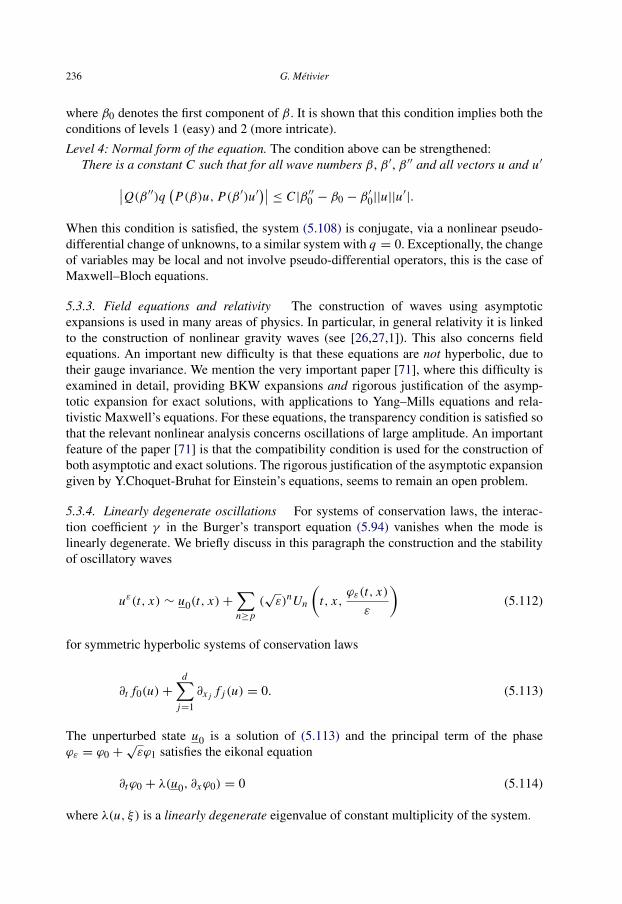
236 G. Metivier
where β0 denotes the first component of β. It is shown that this condition implies both theconditions of levels 1 (easy) and 2 (more intricate).
Level 4: Normal form of the equation. The condition above can be strengthened:There is a constant C such that for all wave numbers β, β ′, β ′′ and all vectors u and u′∣∣Q(β ′′)q (P(β)u, P(β ′)u′
)∣∣ ≤ C |β ′′0 − β0 − β′
0||u||u′|.
When this condition is satisfied, the system (5.108) is conjugate, via a nonlinear pseudo-differential change of unknowns, to a similar system with q = 0. Exceptionally, the changeof variables may be local and not involve pseudo-differential operators, this is the case ofMaxwell–Bloch equations.
5.3.3. Field equations and relativity The construction of waves using asymptoticexpansions is used in many areas of physics. In particular, in general relativity it is linkedto the construction of nonlinear gravity waves (see [26,27,1]). This also concerns fieldequations. An important new difficulty is that these equations are not hyperbolic, due totheir gauge invariance. We mention the very important paper [71], where this difficulty isexamined in detail, providing BKW expansions and rigorous justification of the asymp-totic expansion for exact solutions, with applications to Yang–Mills equations and rela-tivistic Maxwell’s equations. For these equations, the transparency condition is satisfied sothat the relevant nonlinear analysis concerns oscillations of large amplitude. An importantfeature of the paper [71] is that the compatibility condition is used for the construction ofboth asymptotic and exact solutions. The rigorous justification of the asymptotic expansiongiven by Y.Choquet-Bruhat for Einstein’s equations, seems to remain an open problem.
5.3.4. Linearly degenerate oscillations For systems of conservation laws, the interac-tion coefficient γ in the Burger’s transport equation (5.94) vanishes when the mode islinearly degenerate. We briefly discuss in this paragraph the construction and the stabilityof oscillatory waves
uε(t, x) ∼ u0(t, x)+∑n≥p
(√ε)nUn
(t, x,
ϕε(t, x)
ε
)(5.112)
for symmetric hyperbolic systems of conservation laws
∂t f0(u)+d∑
j=1
∂x j f j (u) = 0. (5.113)
The unperturbed state u0 is a solution of (5.113) and the principal term of the phaseϕε = ϕ0 +
√εϕ1 satisfies the eikonal equation
∂tϕ0 + λ(u0, ∂xϕ0) = 0 (5.114)
where λ(u, ξ) is a linearly degenerate eigenvalue of constant multiplicity of the system.

The Mathematics of Nonlinear Optics 237
The standard regime of weakly nonlinear geometric optics corresponds to p = 2.Because of the linear degeneracy, we consider now the case of larger amplitudes corre-sponding to the cases p = 1 and p = 0.
• In space dimension d = 1 and for p = 0, a complete analysis is given in [47] forgas dynamics, and in [62,120,34] in a general framework providing exact solutionswhich admit asymptotic expansions of the form.
• In any dimension, associated with linearly degenerate modes, there always exist sim-ple waves
u(t, x) = v(h(ξ · x − σ t)),
that are exact solutions of (5.113), with v(s) a well-chosen curve defined for s ∈ I ⊂R, ξ and h an arbitrary C1(R; I ) function (cf [103]). Choosing h periodic with periodε, yields exact solutions satisfying (5.112) with p = 0 and associated with the phaseϕ = ξ · x−σ t . The question is to study the stability of such solutions: if one perturbsthe initial data, do the solutions resemble to the unperturbed solutions? We give belowpartial answers, mainly taken from [23,24], but we also refer to [22] for extensions.
1. Existence of BKW solutions for p = 1. It is proved in [23] that in general, one canconstruct asymptotic solutions (5.112) with p = 1, the main oscillation U∗1 being polarizedalong the eigenspace associated with λ. The average u1 of U1 is an arbitrary solution of thelinearized equation from (5.113) at u0. When u1 6= 0, a correction
√εϕ1 must be added to
the phase ϕ0, satisfying
∂tϕ1 + ∂xϕ1 · ∇ξλ(u0, ∂xϕ0)+ u1 · ∇uλ(u0, ∂xϕ0) = 0 (5.115)
so that ϕε = ϕ0 +√εϕ1 satisfies the eikonal equation at the order O(ε), i.e.:
∂tϕε + λ(u0 +√εu1, ∂xϕε) = O(ε). (5.116)
Moreover, the evolution of the main evolution U∗1 is nonlinear (in general) and coupled tothe evolution of the average of U2. The nonlinear regime is reached.
2. Stability / Instability of BKW solutions. In space dimension d = 1, the linear andnonlinear stability is proved using the notion of a good symmetrizer cf [34,62,110,119].When d > 1, the example of gas dynamics shows that the existence of a good symmetrizerdoes not suffice to control oscillations which are transversal to the phase and which canprovoke strong instabilities of Rayleigh type, cf. [54,57].
As before, the question is to know whether the approximate solutions constructed bythe BKW method are close to exact solutions, on some time interval independent of ε. Themain difficulty can be seen from two different angles:
– with uεapp = u0+√εU1(t, x, ϕε/ε)+ . . ., the coefficients f ′j (u
εapp) are not uniformly
Lipschtiz continuous, so that the usual energy method does not provide solutions ona uniform domain,
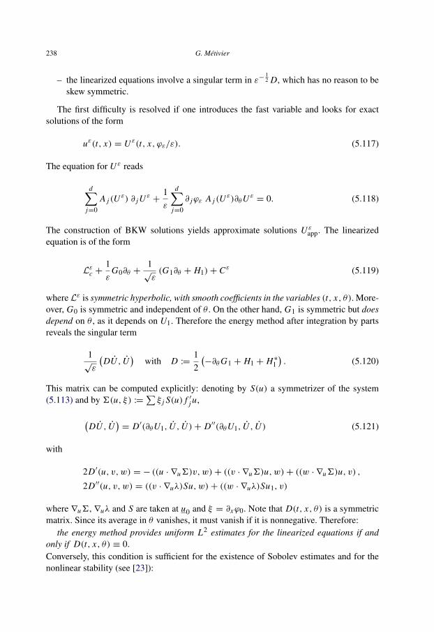
238 G. Metivier
– the linearized equations involve a singular term in ε−12 D, which has no reason to be
skew symmetric.
The first difficulty is resolved if one introduces the fast variable and looks for exactsolutions of the form
uε(t, x) = U ε(t, x, ϕε/ε). (5.117)
The equation for U ε reads
d∑j=0
A j (Uε) ∂ jU
ε+
1ε
d∑j=0
∂ jϕε A j (Uε)∂θU
ε= 0. (5.118)
The construction of BKW solutions yields approximate solutions U εapp. The linearized
equation is of the form
Lεc +
1ε
G0∂θ +1√ε(G1∂θ + H1)+ Cε (5.119)
where Lε is symmetric hyperbolic, with smooth coefficients in the variables (t, x, θ). More-over, G0 is symmetric and independent of θ . On the other hand, G1 is symmetric but doesdepend on θ , as it depends on U1. Therefore the energy method after integration by partsreveals the singular term
1√ε
(DU , U
)with D :=
12
(−∂θG1 + H1 + H∗1
). (5.120)
This matrix can be computed explicitly: denoting by S(u) a symmetrizer of the system(5.113) and by 6(u, ξ) :=
∑ξ j S(u) f ′j u,
(DU , U
)= D′(∂θU1, U , U )+ D′′(∂θU1, U , U ) (5.121)
with
2D′(u, v, w) = − ((u · ∇u6)v,w)+ ((v · ∇u6)u, w)+ ((w · ∇u6)u, v) ,
2D′′(u, v, w) = ((v · ∇uλ)Su, w)+ ((w · ∇uλ)Su1, v)
where ∇u6, ∇uλ and S are taken at u0 and ξ = ∂xϕ0. Note that D(t, x, θ) is a symmetricmatrix. Since its average in θ vanishes, it must vanish if it is nonnegative. Therefore:
the energy method provides uniform L2 estimates for the linearized equations if andonly if D(t, x, θ) ≡ 0.Conversely, this condition is sufficient for the existence of Sobolev estimates and for thenonlinear stability (see [23]):

The Mathematics of Nonlinear Optics 239
THEOREM 5.35. If U εapp is a BKW approximate solution of order εn with n sufficiently
high and if the matrix D vanishes, there are exact solutions U ε of (5.118) such thatU ε−U ε
app = O(εn).
The condition D = 0 is very strong and unrealistic in general, except if U∗1 = 0, inwhich case we recover the standard scaling studied before. In gas dynamics, it is satisfiedwhen the oscillations of U1 concern only the entropy but neither the velocity nor the den-sity: these are what we call entropy waves, but in this case, one can go further and constructoscillations of amplitude O(1) as explained below. Conversely, the Rayleigh instabilitiesstudied in [54] for gas dynamics seem to be the general behavior that one should expectwhen D 6= 0.
3. Entropy waves In contrast to the one dimensional case, D. Serre [119] has shown thatthe construction of O(1) solutions (p = 0) for isentropic gas dynamics yields ill-posedequations for the cascade of profiles. The case of full gas dynamics is quite different: onecan construct O(1) oscillations provided that the main term concerns only the entropy andnot the velocity. Consider the complete system of gas dynamics expressed in the variables(p, v, s), pressure, velocity and entropy:ρ (∂tv + (v · ∇x )v)+∇x p = 0,
α (∂t p + (v · ∇x )p)+ div xv = 0,∂t s + (v · ∇x )s = 0
(5.122)
with ρ(p, s) > 0 and α(p, s) > 0. In [24] (see also [22] for extensions), we prove theexistence and the stability of non-trivial solutions uε = (vε, pε, sε) of the form
vε(t, x) = v0(t, x)+ εV ε(t, x, ϕ(t, x)/ε),
pε(t, x) = p0 + εPε(t, x, ϕ(t, x)/ε),
sε(t, x) = Sε (t, x, ϕ(t, x)/ε)
(5.123)
with V, P and S functions of (t, x, θ), periodic in θ and admitting asymptotic expansions∑εn Vn etc. The unperturbed velocity v0 satisfies the over-determined system
∂tv0 + (v0 · ∇x )v0 = 0, div xv0 = 0,
for instance v0 can be a constant. Moreover, p0 is a constant and the phase ϕ is a smoothreal-valued function satisfying the eikonal equation ∂tϕ + (v0 · ∇x )ϕ = 0. The evolu-tion of the principal term is governed by polarization conditions and a coupled system ofpropagation equations.
For instance, consider the important example where v0 is constant (and we can takev0 = 0 by Galilean transformation). We choose a linear phase function solution of theeikonal equation ∂tϕ = 0, and by rotating the axis we have ϕ(t, x) ≡ x1. The componentsof the velocity are accordingly split into v = (v1, w). For the principal term, the polariza-tion condition requires that the oscillations of the first components of V0 and P0, denotedby V ∗0,1 and P∗0 , vanish. Therefore

240 G. Metivier
vε1(t, x) = εV 0,1(t, x)+ O(ε2),
wε(t, x) = εW0(t, x, x1/ε)+ O(ε2),
pε(t, x) = p0 + εP0(t, x)+ O(ε2),
sε(t, x) = S(t, x, x1/ε)+ O(ε).
The profiles V1(t, x), V2(t, x, θ), P(t, x) and S(t, x, θ) satisfy〈ρ(p0, S)〉∂t V 0,1 + ∂1 P = 0, V0,1|t=0 = a1(x),ρ(p0, S) (∂t W0 + V 0,1∂θW0)+∇
′P = 0, W0|t=0 = a2(x, θ),〈α(p0, S)〉∂t P + ∂1V 0,1 + 〈div′W 〉 = 0, P |t=0 = a3(x),∂t S + V 0,1∂θ S = 0, S|t=0 = a4(x, θ)
where 〈U 〉 denotes the average in θ of the periodic function U (θ), and ∇ ′ and div′ denotethe gradient and the divergence in the variables (x2, . . . , xd), respectively.
5.3.5. Fully nonlinear geometric optics In this paragraph, we push the analysis one stepfurther and consider an example where the amplitude of the oscillation is so large that theeikonal equation for the phase and the propagation equation for the profile are coupled.This example is taken from [95] (see also [127]) and concerns the Klein–Gordon equation
ε2∂2t u − ε2∂2
x u + f (u) = 0 (5.124)
with f (u) = u p, p ∈ N, p > 1 and odd. As in [95] one can consider a much more generalf , which may also depend on (t, x), but for simplicity we restrict the exposition to thiscase. For such equations, the weakly-nonlinear regime concerns solutions of amplitude
O(ε2
p−1 ). Here we look for solutions of amplitude O(1):
uε(t, x) = U ε
(t, x,
ϕ(t, x)
ε
), U ε(t, x, θ) ∼
∑k≥0
εkUk(t, x, θ) (5.125)
with Uk(t, x, θ) periodic in θ . The compatibility or transparency condition which is nec-essary for the construction is stated in Proposition 5.37 below.
Plugging (5.125) into (5.124) yields the following equations
σ 2∂2θU0 + f (U0) = 0,
σ 2∂2θU1 + ∂u f (U0)U1 + T ∂θU0 = 0,
σ 2∂2θUk + ∂u f (U0)Uk + T ∂θUk−1 +�Uk−2 + Rk(x,U0, . . . ,Uk−1) = 0
with � = ∂2t − ∂
2x ,
σ 2= (∂tϕ)
2− (∂xϕ)
2, T := 2ϕ′t∂t − 2ϕ′x∂x +�ϕ. (5.126)
Moreover, the Rk denote smooth functions of their arguments.

The Mathematics of Nonlinear Optics 241
THEOREM 5.36. The profile equations, together with initial conditions, admit solutions{Uk}.
We sketch the first part of the proof taken from [95].(1) Since σ is independent of θ , the first equation is an o.d.e. in θ depending on the
parameter σ . For σ fixed, the solutions depend on two parameters. They are periodic in θ ,the period depending on the energy. Imposing the period equal to 2π determines one of theparameters. Summing up, we see that
the 2π periodic in θ solutions of the first equations are
U0(t, x, θ) = V0(t, x, θ +2(t, x)) = K (σ (t, x), θ +2(t, x)) (5.127)
with 2 an arbitrary phase shift and K (σ, θ) = σ2
p−1 G(θ), where G(θ) is the unique 2π -periodic solution of ∂2
θG + G p= 0 satisfying G ′(0) = 0, G(0) > 0.
(2) The second equation is a linear o.d.e.
LU1 = −T ∂θU0 (5.128)
where L is the linearized operator at U0 from the first equation. The translation invarianceimplies that the kernel of L is not trivial. Indeed, for fixed (t, x), L is self adjoint and ker Lis a one-dimensional space generated by ∂θV0(t, x, ·+2). Therefore, the o.d.e. in U1 has aperiodic solution if and only if the right-hand side is orthogonal to the kernel. There holds
−T ∂θU0(t, x, θ) = −{
T ∂θV0 + X (2)∂2θ V0
}(t, x, θ +2)
where X = 2ϕ′t∂t − 2ϕ′x∂x . Therefore the integrability condition reads∫ 2π
0((T ∂θV0)∂θV0 + Z(2)∂2
θ V0∂θV0) dθ =12
T∫ 2π
0(∂θV0)
2dθ
= 0, (5.129)
that is
∂tϕ∂t J − ∂xϕ∂x J +�ϕ J = 0, (5.130)
where
J (t, x) :=∫ 2π
0(∂θK )2dθ
= σ4
p−1
∫ 2π
0(∂θG(θ))2 dθ
= c((∂tϕ)
2− (∂xϕ)
2) 4
p−1.

242 G. Metivier
Therefore, (5.130) is a second order nonlinear equation in ϕ:
α∂2t ϕ − 2β∂t∂xϕ − γ ∂
2xϕ = 0 (5.131)
with
α =p − 1
2σ 2+ (∂tϕ)
2, β = ∂tϕ ∂xϕ, γ =p − 1
2σ 2− (∂xϕ)
2.
Note that this equation is strictly hyperbolic for σ > 0. It is a substitute for the eikonalequation, but its nature is completely different:ϕ is determined by the nonlinear wave equation (5.131)The compatibility condition (5.129) being satisfied, the solutions of (5.128) are
U1(t, x, θ) = λ1∂θU0 − L−1T (∂θU0) = λ1∂θU0 +W1 (5.132)
where λ1 is an arbitrary function of (t, x) and L−1 denotes the partial inverse on toker L⊥ of the operator L = σ 2∂2
θ + f ′(U0). Note that U1(t, x, θ) is also of the formV1(t, x, θ +2(t, x)).
(3) The third equation is of the form
LU2 = F2 = T ∂θU1 +12
f ′′(U0)U21 +�U0. (5.133)
For this o.d.e in U2, the integrability condition reads
∫ 2π
0F2(t, x, θ)∂θU0(t, x, θ)dθ = 0. (5.134)
Using (5.132), it is an equation for λ1 and 2.
PROPOSITION 5.37 ([95]). If the phase equation (5.130) is satisfied, then the condition(5.134) is independent of λ1 and reduces to a second order hyperbolic equation for 2.
PROOF. The term in λ21 is 1
2
∫ 2π0 f ′′(U0)(∂θU0)
3dθ . The integral vanishes, since the trans-lation invariance implies that(
σ 2∂2θ + f ′(U0)
)∂2θU0 = − f ′′(U0)(∂θU0)
2 (5.135)
implying that the right hand side is orthogonal to ∂θU0.
The linear term in λ1 is∫ 2π
0T (λ1∂
2θU0)∂θU0dθ +
∫ 2π
0λ1 f ′′(U0)(∂θU0)
2W1dθ.

The Mathematics of Nonlinear Optics 243
Using (5.135), the second integral is
−
∫ 2π
0L(∂2
θU0)W1dθ =∫ 2π
0∂2θU0 (T ∂θU0)dθ
so that the linear term is
T
(∫ 2π
0λ1∂
2θU0∂θU0dθ
)= T (0) = 0.
Therefore the condition (5.134) reduces to∫ 2π
0
(T (∂θW1)+
12
f ′′(U )(W1)2+�U0
)∂θU0dθ = 0. (5.136)
There holds
W1(t, x, θ) = −{
L−10 (T ∂θV0)+ X (2)L−1
0 (∂2θ V0)
}(t, x, θ +2),
�U0(t, x, θ) = {�2∂θV0 + ∂t2A + ∂x2B +�V0} (t, x, θ +2)
where L−10 denotes the partial inverse of L0 = σ
2∂2θ + f ′(V0), and A and B depend only
on V0. Therefore, (5.136) is a second order nonlinear equation in2, whose principal part is
�2∫ 2π
0(∂θV0)
2dθ + X22
∫ 2π
0L−1
0 (∂2θ V0)∂
2θ V0dθ.
�
(4) Construction of BKW solutions. The phase ϕ is constructed from (5.131) and suit-able initial conditions. The phase shift2 is given by the nonlinear hyperbolic equation andinitial conditions. This completely determines the principal term U0, U1 up to the choiceof λ1, and U2 is also determined from (5.133) up to a function λ2∂θU0 in the kernel ofL. The fourth equation in the cascade is LU3 = F3 and the compatibility condition is∫ 2π
0 F3∂θU0dθ = 0. It is independent of λ2 and gives an equation for λ1. The proceduregoes on to any order and provides asymptotic solutions (5.125).
The bad point is that these asymptotic solutions are unstable. This has been used byG. Lebeau to prove that the Cauchy problem �u + u p is ill-posed in H s(Rd) in the super-critical case, that is when 1 < s < d
2 −d
p+1 .
THEOREM 5.38 ([95]). The BKW solutions constructed in Theorem 5.36 are unstable.
We just give below an idea of the mechanism of instability. The linearized equation is
ε2(∂2t − ∂
2x )u − f ′(uεapp)u = f . (5.137)
The potential f ′(uεapp) is a perturbation of σ 2 f ′(G(ϕ/ε + 2)). Taking ϕ as a new timevariable or restricting the evolution to times t �
√ε, one can convince oneself that the
relevant model is the equation:

244 G. Metivier
ε2(∂2t − ∂
2x )u + f ′(G(t/ε)u) = f . (5.138)
Setting s = t/ε and performing a Fourier transform in x , reduces to the analysis of the Hilloperator
Mλu :=(∂2
s + f ′(G(s))+ λ)
u, λ = ε2ξ2. (5.139)
Let Eλ(s) denote the 2×2 matrix which describes the evolution of (u, u′) for the solutionsof Mλu = 0. Since the potential f ′(G) is 2π -periodic, the evolution for times s > 2π isgiven by
Eλ(s) = Eλ(s′) (Eλ(2π))k , s = s′ + 2kπ. (5.140)
Therefore, the behavior as s → ∞ is given by the iterates Mkλ , and depends only on the
spectrum of Mλ.
PROPOSITION 5.39 ([95]). There are µ0 > 0 and λ0 > 0 such that eµ0 > 1 is an eigen-value of Mλ0 , and for all λ ≥ 0 the real part of the eigenvalues of Mλ are less than orequal to eµ0 .
This implies that there are initial data such that the homogeneous equation (5.138) withf = 0 has solutions which grow as eµ0t/ε, which are thus larger than any given power ofε in times t = O(ε| ln ε|). This implies that expansion in powers of ε is not robust un-der perturbations, and eventually this implies the nonlinear instability of the approximatesolutions. For the details, see [95].
5.4. Caustics
A major phenomenon in multidimensional propagation is focusing: this occurs when therays of geometric optics accumulate and form an envelope. The phases satisfy eikonalequations,
∂tϕ + λ(t, x, ∂xϕ) = 0 (5.141)
and are given by Hamilton–Jacobi theory. Generically, that is for non-planar planar phases,the rays are not parallel (and curved) and thus have an envelope which is called thecaustic set.
When rays focus, amplitudes grow and, even in the linear case, one must change theasymptotic description. In the nonlinear case, the large amplitudes can be amplified bynonlinearities and therefore strongly nonlinear phenomena can occur.
5.4.1. Example: spherical waves Consider for instance the following wave equation inspace dimension d
� uε + F(∇t,x uε) = 0 (5.142)
The Mathematics of Nonlinear Optics 245
and weakly nonlinear oscillating solutions uε ∼ εU (t, x, ϕ/ε) associated with one of thetwo phases ϕ± = t ± |x |. The propagation of the oscillation of the principal amplitude U0,is given by the following equation for V = ∂θU0:
2(∂t ∓
1|x |
x · ∂x ∓d − 1|x |
)V + F(V∇ϕ±) = 0. (5.143)
• The rays of geometric optics are the integral curves of ∂t ∓∂r , that is the lines x = y∓t y|y| . For ϕ+, all the rays issuing from the circle |y| = a cross, at time t = a, at x = 0.
This is the focusing case (for positive times). The caustic set is C = {x = 0}. For ϕ−,the rays diverge and do not intersect, this is the defocusing case (for positive times).• For linear equations (F = 0), the local density of energy is preserved along the rays
by the linear propagation. This is a general phenomenon when the linear equationshave conserved energy. This means that if F = 0, e(t, x, θ) := |x |d−1
|V (t, x, θ)|2
satisfies
(∂t ∓ ∂r )e = 0. (5.144)
In the focusing case, |x | → 0 when one approaches the caustic set along a ray, and there-fore the conservation of e implies that the intensity |V | → ∞.
• For nonlinear equations, V = rd−1
2 V satisfies
(∂t ∓ ∂r )V + rd−1
2 F(
r−d−1
2 V∇ϕ±)= 0. (5.145)
From here, it is clear that the nonlinearity can amplify or decrease the growth of the am-plitude as r → 0 along the rays. We give several examples.
Example 1: Blow up mechanismsConsider in space dimension d = 3, Eq. (5.142) with F(∇u) = −|∂t u|2∂t u. For the
solution of the focussing equation (5.143) the local energy e(t, x, θ) := |x |2|V (t, x, θ)|2
is satisfied on the ray x = y − t y|y| :
e(t, x, θ) =e(0, y, θ)
1− te(0,y,θ)|x ||y|
, y := x + tx
|x |. (5.146)
Therefore, if V (0, y, θ) 6= 0, even if it is very small, e and V blow up on the ray startingat y, before reaching the caustic set x = 0.
Two mechanisms are conjugated in this example. The first, is due to the nonlinearity−|V |2V , as in the ordinary differential equation V ′ − |V |2V = 0. But for this equation,the blow up time depends on the size of the data. It is very large when the data are small.The second mechanism is the amplification caused by focusing, as in the linear transportequation ∂t V − ∂|x |V − 1
|x |V = 0. Even if the data is small, it forces V to be very large be-

246 G. Metivier
fore one reaches the caustic. Then the first mechanism is launched and the solution blowsup very quickly.
Note that the blow up occurs not only in L∞ but also in L1, before the first time of fo-cusing. It proves that for solutions uε of (5.142), the principal term in the geometric opticsexpansion of ∇uε blows up. This does not prove that ∇uε itself becomes infinite for a fixedε, but at least that it becomes arbitrarily large. This shows that focusing is an essential partof the mechanism which produces large solutions in a finite time bounded independentlyof the smallness of the data.
One can modify the example to provide an example where the exact solution is not ex-tendable, even in the weak sense, after the first time of focusing. Consider in dimensiond = 5, Eq. (5.142) with F(∇u) = (∂t uε)2 − |∇x uε|2 and initial data supported in theannulus {1 < |x | < 2}:
uε(0, x) = 0, ∂t uε(0, x) = U1(x, |x |/ε),
Nirenberg’s linearization, vε := 1 − exp(−uε), transforms the equation into the linearinitial value problem
�vε = 0, vε(0, x) = 0, ∂tvε(0, x) = U1(x, |x |/ε).
The solution vε is defined for all time and vanishes in the cone C := {|x | ≤ 1− t}, but thedomain of definition of uε is �ε, defined as the connected open subset of {vε < 1}, whichcontains C. Focusing make vε arbitrarily large on the focus line {x = 0}, or times t arbitrar-ily close to 1 as ε → 0. One can choose data such that for all δ > 0, if ε is small enough,then the sphere Bδ , of radius δ and centered at (t = 1, x = 0) (the first focusing point), isnot contained in �ε for ε < ε0, and (∂t uε)2 − |∇x uε|2 is not integrable on �ε ∩ Bδ (upto the boundary ∂�ε). In particular, uε cannot be extended to Bδ , even as a weak solution.Thus the first focusing time is the largest common lifetime of the (weak) solutions uε.
These examples taken from [76,79] illustrate that focusing and blow up can be createdin the principal oscillations themselves. This is called direct focusing in [76]. But nonlinearinteractions make the problem much harder. Focusing and blow up can be created by phasesnot present in the principal term of the expansion, but which are generated after several in-teractions. This phenomenon is explored in detail in [76] where it is called hidden focusing.
Example 2: Absorption of oscillationsWhen combined with strongly dissipative mechanisms, focusing can lead to a complete
absorption of oscillations, in finite time. The oscillations disappear when they reach thecaustic set. The following example of such a behaviour is taken from [78]. Consider indimension d = 3, the dissipative wave equation
�u + |∂t u|2∂t u = 0,
with oscillating initial data
uε(0, x) = εU0(x, |x |/ε), ∂t uε(0, x) = U1(x, |x |/ε),
The Mathematics of Nonlinear Optics 247
There are global weak solutions uε ∈ C0([0,∞[; H1) with ∂t uε ∈ C0([0,∞[; L2) ∩
L4([0,∞[×R4) (see [99]). When U0 is even in θ and U1 = ∂θU0, the asymptotic expan-sion of uε is given by
uε(t, x) = εU0(t, x, (|x | + t)/ε)+ ε2 . . . .
and V := ∂θU0 satisfies the transport equation (5.145), which implies that the density ofenergy e(t, x, θ) := |x |2|V (t, x, θ)|2 is also satisfied (compare with (5.146)):
e(t, x, θ) =e(0, y, θ)
1+ te(0,y,θ)|x ||y|
, y := x + tx
|x |.
If V (0, y, θ) 6= 0, then along the ray x = y − t y|y| ,
|V | → +∞, but e→+0 as |x | → 0.
This means that the amplitude V is infinite at the caustic, but the density of energy trans-ported by the oscillations tends to zero, that is, it is entirely dissipated. This suggeststhat the oscillations are absorbed when they reach the caustic set. This is rigourouslyproved in [78].
5.4.2. Focusing before caustics Example 1 of the preceding section illustrates a gen-eral phenomenon. Consider a semi-linear equation and a phase ϕ solution of the eikonalequation (5.141) associated with a simple eigenvalue λ(t, x, ξ) with initial value ϕ0. Thesolution ϕ is constructed by the Hamilton–Jacobi method: the graph of ∂xϕ at time t is theflow out 3 of ∂xϕ0 by Hλ, the Hamiltonian field of λ. The phase ϕ is defined and smoothas long as the projection (x, ξ) 7→ x from 3 ⊂ Rd
× Rd to Rd is a diffeomorphism. Thisis equivalent to requiring that the flow of the Xϕ , the projection of Hλ|3, is a diffeomor-phism. This ceases to be true at the envelope of the integral curves of Xϕ , which is calledthe caustic set C. The transport equation for amplitudes given by geometric optics is ofthe form
∂tU0 +∑
∂ξ j (t, x, ∂xϕ)∂x j U0 + c(t, x)U0 = F(U0). (5.147)
The coefficient c is precisely singular on the caustic set C and becomes singular along therays when one approaches C. Therefore the discussion presented in the example (5.143)can be repeated in this more general context.
5.4.3. Oscillations past caustics
The linear caseIn the linear theory, the exact solutions are smooth and bounded. This means that for
high frequency waves, focusing creates large but not infinite intensities. This is a classi-

248 G. Metivier
cal device to prove that mutli-dimensional hyperbolic equations do not preserve L p normsexcept for p = 2. One idea for studying the behaviour of oscillations near caustics, is toreplace phase-amplitude expansions like (5.9) by Lagrangian integrals (see [43,64,65]).For constant coefficient equations, they are of the form
(2πε)−d∫∫
ei8(t,x,y,ξ)/εa(t, y) dy dξ, (5.148)
where the phase
8(t, x, y, ξ) := −tλ(ξ)+ (x − y) · ξ + ψ(y)
is associated with a smooth piece of the characteristic variety given by the equationτ +λ(ξ) = 0 (see the representation (5.2)). These integrals are associated with Lagrangianmanifolds, 3 ⊂ T ∗R1+d , which are the union of the bi-characteristics
x = y + t∇ξλ(ξ), ξ = dψ(y), τ = −λ(ξ). (5.149)
The projections in (t, x) of these lines are the rays of optics. For small times and as longas it makes sense, Hamilton–Jacobi theory tells us that3 is the graph of dϕ where ϕ is thesolution of the eikonal equation
∂tϕ + λ(∂xϕ) = 0, ϕ|t=0 = ψ.
The projection from 3 to the base is nonsingular at points where the Hessian ∂2y,ξ8 of 8
with respect to the variables (y, ξ) is nonsingular. Therefore the caustic set C associatedwith 3 is
C := {(t, x) : ∃y : x = y + tg(y) and 1(t, y) = 0} (5.150)
where 1(t, y) =∣∣∣det ∂2
y,ξ8
∣∣∣ 12
and g(y) = ∇ξλ(dψ(y)).
The local behaviour of integrals (5.148) is given by stationary phase expansions. Out-side the caustic set, one recovers geometric optics expansions (5.9). The principal term is
∑{y|y+tg(y)=x}
11(t, y)
im(t,y)a(t, y)eiψ(y)/ε (5.151)
where 2m(t, y) is the signature of ∂2y,ξ8. For small times, for each (t, x) there is one critical
point y, ψ(y) = ϕ(t, x) and m = 0. When one approaches the caustic set along the ray, theamplitude tends to infinity, as expected, since 1→ 0, but after the caustic along that ray,one recovers a similar expansion, where the phase has experienced a shift equal to m π
2 .This explains how the geometric optics expansions (5.9) can be recovered from the in-
tegral representation (5.148) and how this representation resolves the singularity present

The Mathematics of Nonlinear Optics 249
in the geometric optics description. It also explains how geometric optics expansions arerecovered after the caustic.
The detailed behavior of oscillatory integrals near the caustic is a complicated and del-icate problem (see [43]). In particular, one issue is to get sharp L∞ bounds, that is themaximum value of intensities, depending on ε. In the simplest case when the singular-ity of the projection of the Lagrangian 3 is a fold, there is good nonsingular asymptoticdescription using Airy functions (see e.g. [101,65]):
uε ={ε−
16 aε(t, x)Ai(σ/ε
23 )+ ε
16 bε(t, x)Ai′(σ/ε
23 )}
eiρ/ε (5.152)
where σ and ρ are two phase functions and the amplitudes aε and bε have asymptoticexpansions
∑εnan and
∑εnbn , respectively. Moreover, the caustic set is {σ = 0}, and
using the asymptotic expansions of the Airy function Ai and its derivative Ai′, one findsthat uε = O(ε∞) in any compact subset of the shadow region {σ > 0}, and that uε isthe superposition of two wave trains (5.9) in any compact subset of the illuminated region
{σ < 0} associated with the phases ρ ± 23 (−σ)
32 .
The nonlinear case• The extension of the previous results to nonlinear equations is not easy and most ques-
tions remain open. An important difficulty is that products of an oscillatory integral like(5.148) involve integrals with more and more variables, hinting that a similar representa-tion of solutions of nonlinear equations would require an infinite number of variables. Thusthis path seems difficult to follow, except if one has some reason to restrict the analysis tothe principal term of the integrals.
This has been done for semi-linear equations with constant coefficients in two cases:for dissipative nonlinearities or when the nonlinear source term is globally Lipschtizean.In these two cases, the structure of the equation implies that one can analyze the exactsolution in low regularity spaces such as L2 or L p and provide asymptotic expansions us-ing oscillatory integrals with small errors in these spaces only (see [79,80]). The naturalextension of (5.148) is
I ε(A) =1
(2πε)d
∫∫e−i(tλ(ξ)+(x−y)ξ)A(t, y, ψ(y)/ε) dy dξ,
associated with profiles
A(t, y, θ) =∑n 6=0
an(t, y)einθ .
There are transport equations for the profile A, which are o.d.e along the lifted raysy + tg(y) in the Lagrangian 3. The phenomenon of absorption is interpreted as the prop-erty that A = 0 past the caustic. It occurs if the dissipation is strong enough. For globallyLipchitzean nonlinearities or weak dissipation, the profile A is continued past the caustic,providing geometric optics approximations at the leading order. Note that in the analogue
250 G. Metivier
of (5.151), the multiplication by im of the amplitude a has to be replaced by Hm A, whereH is the Hilbert transform of the Fourier series
H( ∑
n 6=0
aneinθ
):=
∑n 6=0
i sign naneinθ .
The very weak point of this analysis is that is leaves out completely the case of conservativenon-dissipative equations.• In the same spirit, the use of representations such as (5.152) using Airy functions is
not obvious, since a product of Airy functions is not a Airy function. Such an approachis suggested by J. Hunter and J. Keller in [69] as a technical device to match the geo-metric optics expansions before and after the caustics. Another output of their analysis isa formal classification of the qualitative properties of weakly nonlinear geometric optics,separating linear and nonlinear propagation, and linear and nonlinear effects of the caustic.R. Carles has rigorously explained this classification, mainly for spherical waves, for thewave equations
(∂2t −1x )u + a|∂t u|
p−1∂t u = 0, p > 1; a ∈ C, (5.153)
(a > 0, a < 0, a ∈ iR corresponding to the dissipative, accretive and conservative case,respectively) or the semiclassical nonlinear Schrodinger equation (NLS),
iε∂t u +12ε21x u = εα|u|2σu, u|t=0 = f (x)e−|x |
2/2ε (5.154)
with α ≥ 1, σ > 0.In [12], for 1 < p < 2, the reader can find an L∞ description near x = 0 of radial
waves in R3 for (5.153). As expected, the profiles and the solutions are unbounded (uni-formly in ε) and new amplitudes (of size ε1−p) must be added to the one predicted in [69]as correctors near the caustic in order to have a uniform approximation in L∞. In particular,this gives the correct evaluation of the exact solutions at the caustic set {x = 0}.
Concerning NLS, R. Carles has investigated all the behaviors with different powersα ≥ 1 and σ > 0.
– When α > dσ and α > 1, the propagation of the main term ignores the nonlinearity,outside the caustic and at the caustic.
– When α = 1 > dσ , the propagation before and after the caustic follows the rule ofweakly nonlinear optics, and the matching at the focal point is like in the linear case.
– When α = dσ > 1, the nonlinear effects take place only near the focal point. Aremarkable new idea is that the transition between the amplitudes before and afterthe focal point is given a scattering operator.
We refer the reader to [13–15] for details.
The Mathematics of Nonlinear Optics 251
6. Diffractive optics
The regime of geometric optics is not adapted to the propagation of laser beams in dis-tances that are much larger than the width of the beam. The standard descriptions that canbe found in physics text books involve Schrodinger equations, used to model the diffrac-tion of light in the direction transversal to the beam along long distances. The goal ofthis section is to clarify the nature and range of validity of the approximations leading toSchrodinger-like equations, using simple models and examples.
6.1. The origin of the Schrodinger equation
6.1.1. A linear example Consider again a symmetric hyperbolic linear system (5.1) withconstant coefficients and eigenvalues of constant multiplicities. Consider oscillatory initialdata (5.3). The solution is computed by Fourier synthesis, as explained in (5.4), revealingintegrals
uεp(t, x)=1
(2π)d/2
∫ei{y(k+εξ)−tλp(k+εξ)}/ε5p(k + εξ)h(ξ)dξ
= ei(kx−tωp)/εaεp(t, x). (6.1)
The error estimates (5.6) show that the approximation of geometric optics is valid as longas t = o(1/ε). To study times and distances of order 1/ε, insert the second order Taylorexpansion
λp(k + εξ) = ωp + εξvp + ε2Sp(ξ)+ O(ε3
|ξ |3),
with
Sp(ξ) :=12
∑j,k
∂2ξ j ,ξk
λp(k)ξ jξk, (6.2)
into the integral (6.1) to find
aεp(t, x) =1
(2π)d/2
∫ei(xξ−tξvp)e−iεt Sp(ξ)5p(k)h(ξ)dξ + O(ε2t)+ O(ε).
Introduce the slow variable T := εt and
ap,0(T, t, y) :=1
(2π)d/2
∫ei(xξ−tξvp)e−iT Sp(ξ)5p(k)h(ξ)dξ. (6.3)
Then ∥∥∥aεp(t, ·)− ap,0(εt, t, ·)∥∥∥
H s (Rd )≤ C(ε2t + ε) ‖h‖H s+3(Rd ) . (6.4)

252 G. Metivier
The profile ap,0 satisfies the polarization conditions ap,0 = 5p(k)ap,0 and a pair of partialdifferential equations:
(∂t + vp · ∇x )ap,0 = 0, and(i∂T + Sp(∂x )
)ap,0 = 0. (6.5)
The first is the transport equation of geometric optics and the second is the Schrodingerequation, with evolution governed by the slow time T , which we were looking for. These,together with the initial condition
ap,0(0, 0, y) = f (y),
suffice to uniquely determine ap,0.Note that for t = o(1/ε) one has T → 0, and setting T = 0 in (6.3) one recovers
the approximation of geometric optics. A typical solution of the Schodinger equation hasspatial width which grows linearly in T (think of Gaussian solutions). Thus the typicalwidth of our solution uε grows linearly in εt , which is consistent with the geometric obser-vation that the wave vectors comprising u|t=0 = heikx/ε make an angle O(ε) with k. Theapproximation (6.4) clearly presents three scales; the wavelength ε, the lengths of order 1on which f varies, and, the lengths of order 1/ε traveled by the wave on the time scales ofthe variations of ap with respect to the slow time T .
In contrast to the case of the geometric optics expansion, the analysis above does notextend to non-planar phases ϕ(t, x)/ε. Note that the rays associated with nonlinear phasesfocus or spread in times O(1). The case of focusing of rays and its consequences for non-linear waves was briefly discussed in Section 5. On the other hand, with suitable convexityhypotheses on the wavefronts, nonlinear transport equations along spreading rays yieldnonlinear geometric optics approximations valid globally in time (see [56]). In the sameway, one does not find such Schrodinger approximations for linear phases when the geo-metric approximations are not governed by transport equations. The classical example isconical refraction.
However, the analysis does extend to phases (kx − ωt + ψ(εt, εx)) /ε with slowlyvarying differentials, observing that for times t . ε−1 the rays remain almost parallel.We refer to [67,45] for these extensions.
CONCLUSION 6.1. The Schrodinger approximations provide diffractive corrections fortimes t ∼ 1/ε to solutions of wavelength ε which are adequately described by geometricoptics with parallel rays for times t ∼ 1.
These key features, parallel rays and three scales, are commonly satisfied by laserbeams. The beam is comprised of virtually parallel rays. A typical example with threescales would have wavelength ∼ 10−6 m, the width of the beam ∼ 10−3 m, and the prop-agation distance ∼ 1 m.
6.1.2. Formulating the Ansatz For simplicity, we study solutions of semi-linear sym-metric hyperbolic systems with constant coefficients and nonlinearity which is or order J

The Mathematics of Nonlinear Optics 253
near u = 0. The quasi-linear case can be treated similarly. Consider
L(ε∂) = εA0∂t +
d∑j=1
εA j∂x j + E (6.6)
with self-adjoint matrices A j , A0 being positive definite, and with E skew-adjoint. Thenonlinear differential equation to solve is
Lε(∂x )uε+ F(uε) = 0 (6.7)
where uε is a family of CN valued functions. The nonlinear interaction term F is assumedto be a smooth nonlinear function of u and of order J ≥ 2 at the origin, in the sense thatthe Taylor expansion at the origin satisfies
F(u) = 8(u)+ O(|u|J+1) (6.8)
where 8 is a homogeneous polynomial of degree J in u, u.
Time of nonlinear interaction and amplitude of the solution. The amplitude of nonlinearwaves in crucially important. Our solutions have amplitude uε = O(ε p) where the expo-nent p > 0 is chosen so that the nonlinear term F(u) = O(ε pJ ) affects the principal termin the asymptotic expansion for times of order 1/ε. The time of nonlinear interaction iscomparable to the times for the onset of diffractive effects.
The time of nonlinear interaction is estimated as follows. Denote by S(t) the propagatorfor the linear operator Lε. Then in L2(Rd), ‖S(t)‖ ≤ C . The Duhamel representation
u(t) = S(t)u(0)−∫ t
0S(t − σ)F(u(σ )) dσ
suggests that the contribution of the nonlinear term at time t is of order tε pJ . For the onsetof diffraction, t ∼ 1/ε so the accumulated effect is expected to be O(ε pJ−2) (note that thecoefficient of ∂t is ε). For this to be comparable to the size of the solution we choose p sothat pJ − 2 = p:
p =2
J − 1. (6.9)
The basic Ansatz. It has three scales
uε(x) = ε pa(ε, εt, εx, t, x, ϕ(t, x)/ε) (6.10)
where ϕ(t, x) = kx − tω and a(ε, T, X, t, x, θ) is periodic in θ and has an expansion:
a = a0 + εa1 + ε2a2 + . . . . (6.11)

254 G. Metivier
Since this expansion is used for times t ∼ 1/ε, in order for the correctors εa1 and ε2a2to be smaller than the principal term for such times, one must control the growth of theprofiles in t . The most favorable case would be that they are uniformly bounded forεt ≤ T0, but this is not always the case as will be shown in the analysis below. There-fore we impose the weaker condition of sublinear growth:
limt→∞
1t
supT,X,y,θ
|a1(T, X, t, x, θ)| = 0. (6.12)
This condition plays a central role in the analysis to follow.
6.1.3. First equations for the profiles Plugging (6.10) into the equation and ordering inpowers of ε yields the equations
L(β∂θ )a0 = 0, (6.13)
L(β∂θ )a1 + L1(∂t,x )a0 = 0, (6.14)
L(β∂θ )a2 + L1(∂t,x )a1 + L1(∂T,X )a0 +8(a0) = 0 (6.15)
with β = dϕ = (−ω, k) and L(β∂θ ) = L1(β)∂θ + E .
Analysis of Eqs (6.13) and (6.14). The first two equations are those met in the geomet-ric optics regime. They are analyzed using Fourier series expansions in θ . We make thefollowing assumptions, satisfied in many applications:
ASSUMPTION 6.2. (i) β satisfies the dispersion relation
det(L1(β)− iE) = 0. (6.16)
Denote by Z the set of harmonics n ∈ Z such that det(L1(nβ)− iE) = 0.(ii) If E 6= 0, det(L1(β)) 6= 0, so that Z is finite.
(iii) For n ∈ Z , n 6= 0, the point nβ is a regular point in the characteristic set in thesense of Definitions 5.3.
As in Section 5, we denote by P and Q projectors on the kernel and the image ofL(β∂θ ), respectively, and by R the partial inverse such that
RL(β∂θ ) = Id − P, P R = 0, R(Id −Q) = 0. (6.17)
They are defined by projectors Pn and Qn and partial inverses Rn acting on the Fouriercoefficients an of Fourier series
∑aneinθ .
The first equation asserts that the principal profile is polarized along the kernel ofL(β∂θ ):
a0 = P a0 ⇔ ∀n, a0,n = Pn a0,n . (6.18)
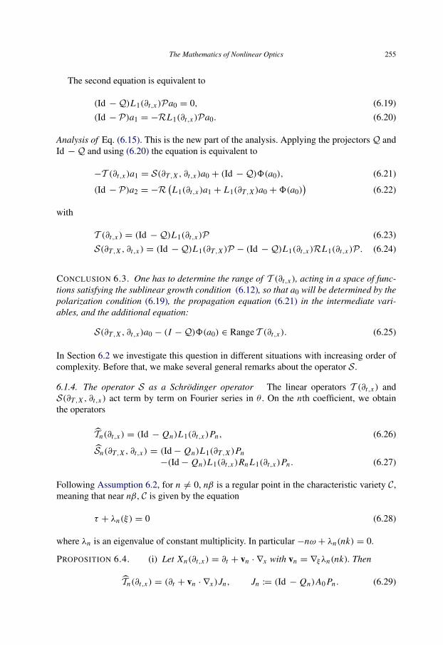
The Mathematics of Nonlinear Optics 255
The second equation is equivalent to
(Id −Q)L1(∂t,x )P a0 = 0, (6.19)
(Id − P)a1 = −RL1(∂t,x )P a0. (6.20)
Analysis of Eq. (6.15). This is the new part of the analysis. Applying the projectors Q andId −Q and using (6.20) the equation is equivalent to
−T (∂t,x )a1 = S(∂T,X , ∂t,x )a0 + (Id −Q)8(a0), (6.21)
(Id − P)a2 = −R(L1(∂t,x )a1 + L1(∂T,X )a0 +8(a0)
)(6.22)
with
T (∂t,x ) = (Id −Q)L1(∂t,x )P (6.23)
S(∂T,X , ∂t,x ) = (Id −Q)L1(∂T,X )P − (Id −Q)L1(∂t,x )RL1(∂t,x )P. (6.24)
CONCLUSION 6.3. One has to determine the range of T (∂t,x ), acting in a space of func-tions satisfying the sublinear growth condition (6.12), so that a0 will be determined by thepolarization condition (6.19), the propagation equation (6.21) in the intermediate vari-ables, and the additional equation:
S(∂T,X , ∂t,x )a0 − (I −Q)8(a0) ∈ Range T (∂t,x ). (6.25)
In Section 6.2 we investigate this question in different situations with increasing order ofcomplexity. Before that, we make several general remarks about the operator S .
6.1.4. The operator S as a Schrodinger operator The linear operators T (∂t,x ) andS(∂T,X , ∂t,x ) act term by term on Fourier series in θ . On the nth coefficient, we obtainthe operators
Tn(∂t,x ) = (Id − Qn)L1(∂t,x )Pn, (6.26)
Sn(∂T,X , ∂t,x ) = (Id− Qn)L1(∂T,X )Pn−(Id− Qn)L1(∂t,x )Rn L1(∂t,x )Pn . (6.27)
Following Assumption 6.2, for n 6= 0, nβ is a regular point in the characteristic variety C,meaning that near nβ, C is given by the equation
τ + λn(ξ) = 0 (6.28)
where λn is an eigenvalue of constant multiplicity. In particular −nω + λn(nk) = 0.
PROPOSITION 6.4. (i) Let Xn(∂t,x ) = ∂t + vn · ∇x with vn = ∇ξλn(nk). Then
Tn(∂t,x ) = (∂t + vn · ∇x )Jn, Jn := (Id − Qn)A0 Pn . (6.29)

256 G. Metivier
(ii) Let
Sn(∂x ) :=12
∑j,k
∂2ξ j ξk
λn(nk)∂x j ∂xk . (6.30)
Then
Sn(∂T,X , ∂t,x ) = (∂T + vn · ∇X − iSn(∂x )) Jn + Rn(∂t,x )Xn(∂t,x ) (6.31)
where Rn is a first order operator which is specified below.
PROOF. Consider n = 1 and drop the indices n. The first part is proved in Lemma 5.9.Recall that differentiating the identity(
−iλ(ξ)A0 +∑
j
iξ j A j + E
)P(ξ) = 0
once, yields(−iλ(ξ)A0 +
∑j
iξ j A j + E
)∂ξp P(ξ) = −i(−∂ξpλ(ξ)A0 + Ap)P(ξ).
Multiplying on the left by Id − Q(k) implies
(Id − Q(k))(−∂ξpλ(k)A0 + Ap)P(k) = 0, (6.32)
(Id − P(k))∂ξp P(k) = −iR(k)(−∂ξpλ(k)A0 + Ap)P(k). (6.33)
The first identity implies (6.29).
Differentiating the identity again and multiplying on the left by Id − Q(k) implies that
(Id − Q)(−∂ξpλA0 + Ap)∂ξq P + (Id − Q)(−∂ξqλA0 + Aq)∂ξp P
= ∂2ξp,ξq
λ(Id − Q)A0 P
where the functions are evaluated at ξ = k. Using (6.32), one can replace ∂ξp P by(Id − P)∂ξp p in the identity above. With (6.33), this implies that
(Id − Q)(−∂ξpλA0 + Ap)R(−∂ξqλA0 + Aq)P
+ (Id − Q)(−∂ξqλA0 + Aq)R(−∂ξpλA0 + Ap)P
= i∂2ξp,ξq
λ (Id − Q)A0 P.
Together with the identity
L1(∂t , ∂x ) = A0(∂t + v · ∇x )+
d∑p=1
(Ap − ∂ξpλA0)∂x p = A0 X (∂t,x )+ L ′1(∂x )

The Mathematics of Nonlinear Optics 257
this implies that
(Id − Q)L1(∂t,x )RL1(∂t,x )P = (Id − Q)X (∂t,x )RL1(∂t,x )P
+ (Id − Q)L ′1(∂x )R X (∂t,x )P
+i2λ (Id − Q)A0 P
∑∂2ξp,ξq
∂x p∂xq
implying (6.31). �
COROLLARY 6.5. If a(T, X, t, x) satisfies the polarization condition a = Pna and thetransport equation X (∂t,x a) = 0, then
Sn(∂T,X , ∂t,x )a = Jn (∂T + v · ∇X + iSn(∂x )) a.
The conclusion is that for all frequency n, the operator Sn acting on the polarized vectorsa is the Shrodinger operator ∂T + v · ∇X + iSn(∂x ), that is, for functions independent of X ,the operator (6.5).
6.2. Construction of solutions
We consider first the simplest case:
6.2.1. The non-dispersive case with odd nonlinearities and odd profiles We assume herethat in Eq. (6.7), E = 0 and F(u) is an odd function of u with a nontrivial cubic term, thatis with J = 3, so that we choose p = 1 according to the rule (6.9). We look for solutions
uε(t, x) ∼ ε∑n≥0
εnan(εt, t, x, ϕ(t, x)/ε), (6.34)
where ϕ(t, x) = kx − tω and the profiles an(T, t, x, θ) are periodic and odd in θ .We assume that ϕ is a characteristic phase and, more precisely, we assume that dϕ is a
regular point of the characteristic variety det L(τ, ξ) = 0. We introduce projectors P andQ on the kernel and on the image of L(dϕ), respectively, and we denote by R the partialinverse of L(dϕ)with properties as above. We denote by X (∂t,x ) = ∂t+v·∇x the transportoperator and similarly by S(∂t,x ) the second order operator (6.2) or (6.30) associated withdϕ. By homogeneity, all the harmonics nϕ, n 6= 0 are characteristic and one can choosethe projectors Pn to be equal to P , Qn = Q. Moreover, all the transport fields have thesame speed and Xn(∂t,x ) = X (∂t,x ). Similarly, Sn(∂x ) = S(∂x ).
Because we postulate that a0 is odd in θ , its zeroth harmonic (its mean value) vanishes.Therefore, the polarization condition (6.20) reduces to
a0(T, t, x, θ) = Pa0(T, t, x, θ), (6.35)
and the first condition Eq. (6.19) reads
(∂t + v∇x )a0(T, t, x, θ) = 0. (6.36)

258 G. Metivier
Because we also postulate that a1 is odd, (6.20) is equivalent to
(Id − P)a1(T, t, x, θ) = −∂−1θ RL1(∂t,x )Pa0 (6.37)
where ∂−1θ is the inverse of ∂θ acting on functions with a vanishing mean value. Next, Eq.
(6.21) is
−(∂t + v∇x )(Id − Q)A0 Pa1 = (Id − Q)8(a0)+ ∂T (Id − Q)A0 Pa0
− (Id − Q)L1(∂t , x)∂−1θ RL1(∂t,x )P, (6.38)
where we have used the following remark:
if 8 is odd in u and if a0 is odd in θ, then 8(a0) is odd in θ, (6.39)
implying that the mean value of 8(a0) vanishes and that Q8(a0) = Q8(a0).Next we note that the scalar operator X (∂t,x ) commutes with all the constant coefficient
operators in the right-hand side of (6.38) so that (6.36) implies that the right-hand side f0
of (6.38) satisfies
X (∂t,x ) f0 = 0, (6.40)
and the equation for a1 = (Id − Q)A0 Pa1 reduces to
X (∂t,x )a1 = f0. (6.41)
By (6.40), f0 is constant along the rays of X , and thus a1 is affine on these rays. Therefore,
LEMMA 6.6. If f0 satisfies (6.40), Eq. (6.41) has a solution with sublinear growth in t, ifand only if f0 = 0. In this case, the solutions a1 are bounded in time.
Therefore, we see that Eq. (6.38) has a solution a1 with sublinear growth in t , if and onlyif the following two equations are satisfied:
(Id − Q)8(a0)+ ∂T (Id − Q)A0 Pa0
− (Id − Q)L1(∂t , x)∂−1θ RL1(∂t,x )P = 0, (6.42)
(∂t + v∇x )Pa1 = 0. (6.43)
Moreover, using Proposition 6.4, we see that for a0 satisfying (6.36), the first equation isequivalent to
∂T a0 + ∂−1θ S(∂x )a0 = R08(a0) (6.44)

The Mathematics of Nonlinear Optics 259
where R0 is the inverse of (Id −Q)A0 P from the image of (Id −Q) to the image of P . Onthe harmonic 1, ∂−1
θ = −i, and we recover a Schrodinger equation as in (6.5), now with asource term.
PROPOSITION 6.7 (Existence of the principal profile). Given a Cauchy data h0(x, θ), inH s(Rd
×T), with s > d+12 , odd in θ and satisfying h0 = Ph0, there is T∗ > 0 such that the
two times problem (6.36), (6.44) has a unique solution a0 ∈ C0([0, T∗]×R; H s(Rd×T)),
odd in θ and satisfying a0 = Pa0 and
a0(0, 0, x, θ) = h0(x, θ). (6.45)
PROOF. By the first equation we look for a0 as a function of x − tv
a0(T, t, x, θ) = a0(T, x − tv, θ). (6.46)
Then the equation for a0(T, y, θ) is:
∂T a0 + ∂−1θ S(∂y)a0 + R08(a0) = 0, a0(0, y, θ) = h(y, θ). (6.47)
This equation is quite similar to classical nonlinear Schrodinger equations, ∂−1θ being
bounded and skew-adjoint. Thus it has a local solution in H s , if s is large enough. Theonly point is to check that all the terms in the equations preserve oddness. �
Next we show that (6.37), (6.46) and (6.43) imply that a1 is of the form
a1(T, t, x, θ) = a1(T, x − tv, θ) (6.48)
with (I − P)a1 determined by a0 and thus odd in θ .In the expansion in powers of ε of the equation, the term coming after (6.15) is
L(β∂θ )a3 + L1(∂t,x )a2 + L1(DT,X )a1 +8′(a0)a1 = 0
(Recall that F is odd, so F(u) = ε38(a0)+ε48′0(a0)a1+O(ε5)). Projecting with (Id−Q)
and Q, using the facts that (Id−P)a1 is known, that Pa1 satisfies (6.43) and that (Id−P)a2is given by (6.22), we see that the equation is equivalent to
−(∂t + v∇x )(Id − Q)A0 Pa2 = (∂T + ∂−1θ S(∂x ))(Id − Q)A0 Pa1
+ (Id − Q)8′(a0)Pa1 + (Id − Q)b0
where b0 is determined by a0, together with an explicit determination of (Id − P)a3 interms of a0, a1, a2. In particular, b0(T, t, x, θ) = b0(T, x − tv, θ) with b0 odd in θ . Theright-hand side f1 satisfies (∂t + v∇x ) f1 = 0. Therefore, using Lemma 6.6, we see that a2has a sublinear growth in t if and only if
(∂t + v∇x )Pa2 = 0, (6.49)

260 G. Metivier
and Pa1(T, t, x, θ) = Pa1(T, x − tv, θ) is therefore determined by the equation
∂T a1 + ∂−1θ S(∂y)a1 + R08
′(a0)a1 + R0b0 = 0. (6.50)
The equations for the higher profiles are derived in a similar fashion. We see that theprofiles an in (6.34) have the form an(T, t, x, θ) = an(T, x − tv, θ), so that
uε(t, x) ∼ ε∑n≥0
εnan(εt, x − tv, ϕ(t, x)/ε). (6.51)
The (I − P)aa are determined explicitly in terms of (a0, . . . , an−1) and the slow dynamicsfor Pan is determined by an equation of the form
∂T an + ∂−1θ S(∂y)an + R08
′(a0)an + R0bn−1 = 0 (6.52)
with bn−1 explicitly given in terms of (a0, . . . , an−1).
THEOREM 6.8 (Existence of profiles at all orders). Suppose that for all n ∈ N, initialdata hn ∈ S(Rd
× T) are given, odd in θ and satisfying Phn = hn . Then there existsT∗ ∈ ]0,∞] and a unique sequence {an}n≥0 of functions in S([0, T∗] ×Rd
× T), odd in θand satisfying the profile equations and the initial conditions Pan(0, y, θ) = Phn(y, θ).
Given such a sequence of profiles, Borel’s theorem constructs
aε(T, y, θ) ∼∑n≥0
εnan(T, y, θ)
in the sense that for all s and m ∈ N, there holds for all ε ∈ ]0, 1]:∥∥∥∥∥aε −∑j≤m
ε j a j
∥∥∥∥∥H s ([0,T∗]×Rd×T)
≤ Cs,mεm+1.
Then
uεapp(t, x) := εaε(εt, x − tv, ϕ(t, x)/ε)
are approximate solutions of (6.7), in the sense that
L(ε∂t,x )uεapp + F(uεapp) = rε(εt, x − tv, ϕ(t, x)/ε),
with rε ∼ 0 in the sense above.Using Theorem 4.21 ([59], see also [39,40]), one can produce exact solutions which
have the asymptotic expansion (6.51). Consider initial data
hε(x) ∼ uεapp(0, x) ∼ ε∑n≥0
εnan(0, x, ϕ(0, x)/ε).

The Mathematics of Nonlinear Optics 261
THEOREM 6.9 (Exact solutions). If ε is small enough, the Cauchy problem for (6.7) withinitial data hε has a unique solution uε ∈ S([0, T∗/ε] × Rd) which satisfies for all s, mand ε: ∥∥∥uε − uεapp
∥∥∥H s≤ Cs,mε
m .
6.2.2. Dispersive equations; the Schrodinger equation as a generic model for diffractiveoptics Consider now the case of a dispersive equation (6.7) with E 6= 0 in (6.6). Assumethat the matrices A j are real symmetric and that E is real skew symmetric, as usual in phys-ical applications. Therefore the characteristic polynomial p(τ, ξ) = det(τ A0 +
∑ξ j A j −
iE) is real, and thus equal to det(τ A0 +∑ξ j A j + iE). This implies that p(−τ,−ξ) =
(−1)N p(τ, ξ) so that the characteristic variety C = {p = 0} is symmetric, i.e. −C = C.We fix a planar phase ϕ with β = dϕ = (−ω, k) satisfying Assumption 6.2. We assume
that only the harmonics nβ with n ∈ {−1, 0, 1} are characteristic. We further assume thatthe nonlinearity F is odd, with a nontrivial cubic term 8. Again, we look for solutionsuε of the form (6.34), with profiles an(T, t, x, θ) which are odd in θ , so that the charac-teristic phase 0 never shows up in the computations. All these assumptions are realistic inapplications.
Note that the symmetry assumption of the characteristic variety implies that the eigen-values λ± which describe the characteristic variety C near±β (see (6.28)) satisfy the prop-erty that
λ−(ξ) = −λ+(−ξ). (6.53)
In particular, the group velocities v± = ∇λ±(±k) are equal. We denote their commonvalue by v.
The projector P on ker L(β∂θ ) acting on odd functions reduces to
P( ∑
k∈1+2Zakeikθ
)= P−a−1e−iθ
+ P+a1eiθ
where P± are projectors on ker L(±iβ). Since L(−iβ) = L(iβ), one can choose P− = P+,and choose similarly projectors Q− = Q+ on the images of L(±iβ) and partial inversesR− = R+.
All that which has been done in the non-dispersive case can be repeated in this frame-work: one can construct asymptotic solutions
uε(t, x) ∼ ε∑n≥0
εnan(εt, x − tv, ϕ(t, x)/ε), (6.54)
with profiles an which are odd in θ . They are determined inductively. The Fourier coeffi-cients an ,k for k 6= ±1 and (Id − P±)an ,±1 are given by explicit formulas and P±an ,±1are given by solving a Schrodinger equation.

262 G. Metivier
In particular, the main term contains only the harmonics ±1
a0(T, t, x) = a0,−1(T, t, x)e−iθ+ a0,+1(T, t, x)eiθ (6.55)
satisfying the polarization conditions:
a0,±1(T, t, x) = P±a0,±1(T, t, x) (6.56)
and the propagation equations
∂T a0,±1 ∓ iS(∂y)a0,±1 + B±8(a0)±1 = 0 (6.57)
where B± denotes the partial inverse of (Id Q±)A0 P± on the image of P±. Denoting by8(u, v, w) the symmetric trilinear mapping such that 8(u) = 8(u, u, u), the harmonic of8(a0) is
8(a0)1 = 8(a0,−1a0,1, a0,1
), (6.58)
and there is a similar formula for 8(a0)−1.This is the usual cubic Shrodinger equation for nonlinear optics that can be found in
physics books (see e.g. [6,8,10,107,109]).The BKW solutions provide approximate solutions of the equations, which can be con-
verted into exact solutions, exactly as in Theorem 6.9. This mathematical analysis was firstmade in [39]. We refer to this paper for explicit examples coming from various models innonlinear optics, as discussed in Section 2.
6.2.3. Rectification In the two analyses above, two facts were essential:
• Only regular phases were present. In applications, this excludes the harmonic 0. Thiswas made possible by assuming that both the nonlinearity F and the profiles a wereodd. When F is not odd, for instance when F is quadratic, the harmonic 0 is expectedto be present. In general, and certainly for non-disoersive equations, 0 is not a regularpoint of the characteristic variety, implying that there will be no simple analogue ofLemma 6.6. The creation of a nontrivial mean value field by nonlinear interaction ofwaves is called rectification.• All the characteristic harmonics kβ are regular and have the same group velocities
vk . If not, the Fourier coefficients an ,k are expected to travel at different speeds vk ,so that the right-hand sides in equations like (6.21) or (6.37) have no definite propa-gation speed. In this case too, Lemma 6.6 must be revisited.
We now give the general principles which yield the construction of the principal profilea0, referring to [81,90] for precise statements and proofs.
For a general Eq. (6.7), with F satisfying (6.10), we look for solutions of the form
uε(t, x) = ε paε(εt, t, x, ϕ/ε) (6.59)

The Mathematics of Nonlinear Optics 263
with aε = a0 + εa1 + ε2a2 and ϕ a planar phase with β = dϕ satisfying Assumption 6.2.
The polarization condition (6.18) and the first Eq. (6.19) for a0 are such that its Fouriercoefficients a0,k satisfy Pk a0,k = a0,k and
H0(∂t,x )a0,0 = 0, (6.60)
(∂t + vk · ∇x )a0,k = 0, k 6= 0 (6.61)
where H0 = (Id −Q0)L1(∂t,x )P0. Moreover, the components (Id − Pk)a1,k of the Fouriercoefficients of a1 are given by (6.20):
a1,k = −Rk L1(∂t,x )Pk a0,k . (6.62)
Next, the equations for Pk a1,k deduced from (6.21) read
H0(∂t,x )P0a1,0 + f0,0 = 0, (6.63)
(∂t + vk · ∇x )Pk a1,k + f0,k = 0, k 6= 0, (6.64)
where
f0,k = (Id − Qk)(A0∂T )− L1(∂t,x )Rk L1(∂t,x )Pk a0,k + (Id − Qk)8(a0)k .
We recall that the main problem is to find conditions on the f0,k which imply that theequations for Pk a1,k have solutions with sublinear growth in time. This is what we brieflydiscuss below.
1. Large time asymptotics for homogeneous hyperbolic equationsThe operator H0 is symmetric hyperbolic (on the image of P0) with constant coeffi-
cients. For instance, in the non-dispersive case, E = 0, P = Id and H0 = L1. This leadsone to consider the large time asymptotics of solutions of
H(∂t,x )a = f, a|t=0 = h (6.65)
when H is a symmetric hyperbolic constant coefficient first order system. The character-istic variety C H is a homogeneous algebraic manifold. It may contain hyperplanes, sayCα = {(τ, ξ), τ + cα · ξ = 0}. This does happen for instance for the Euler equation.The flat part Cflat of C H is the union of the Cα . We denote by πα(ξ) the spectral projectoron ker H(−cα · ξ, ξ) and by πα(Dx ) the corresponding Fourier multiplier. The followinglemma is easily obtained by using the Fourier transform of the equation.
LEMMA 6.10. Suppose that h ∈ S(Rd) and a is the solution of the initial value problemH(∂t,x )a = 0, a|t=0 = h. Then
limt→∞
∥∥∥a(t, ·)−∑
(πα(Dx )h) (· − tcα)∥∥∥
L∞(Rd )= 0.

264 G. Metivier
2. Large time asymptotics for 8(a0)
For harmonics k 6= 1, the transport Eq. (6.61) implies that a0,k is a function of x−tvk . Inthe dispersive case, there is a finite number of frequencies k in play; in the non-dispersivecase, all the speeds vk are equal. Thus, in all cases, a finite number of speeds vk occur, andthe Fourier coefficients of a0 are the sum of rigid waves moving at the speed cα or vk andof spreading waves which tends to 0 at infinity. The Fourier component 8(a0),k appears asa sum of products of such waves. Two principles can be observed:
– the product of rigid waves moving at different speeds tends to 0 at infinity;– the product of a spreading wave and anything bounded, also tends to 0 at infinity.
This implies that for all T , the coefficients f0,k have the form
g(t, x) =∑
g j (x − tw j )+ g0(t, x) (6.66)
where the set of speeds is {w j } = {vk} ∪ {cα}, and g0(t, ·) tends to 0 in H s as t → ∞,uniformly in T .
3. Large time asymptotics for inhomogeneous hyperbolic equationsUsing the equation on the Fourier side, one proves the following estimate:
LEMMA 6.11. Consider g as in (6.66). The solution of H(∂t,x )a = g, a|t=0 = 0 satisfies
limt→∞
1t
∥∥∥∥∥∥a(t, ·)− t∑α
∑{ j :w j=cα}
πα(Dx )g j (· − tcα)
∥∥∥∥∥∥L∞(Rd )
= 0.
In particular, there is a solution with sublinear growth if and only if
πα(∂x )g j = 0 when w j = cα. (6.67)
Applied to H = ∂t + vk · ∇x , this lemma implies that the equation (∂t + vk · ∇x )a = ghas a solution with sublinear growth if and only if
g j = 0 when w j = vk . (6.68)
These principles can be applied to the equations (6.63) (6.64) to derive (necessary and)sufficient conditions for the existence of solutions with sublinear growth. These conditionsgive the desired equations for a0. Their form depends on the relations between the speedsvk and cα . To give an example, we consider a particular, simple case and refer to [81,90]for more general statements.
Consider a non-dispersive system. Denote by v the common value of the propagationspeeds vk for k 6= 0. Assume that there is one hyperplane in the characteristic variety of L1,with speed c and projector π . The principal profile a0 is split into its mean value 〈a0〉 = a0and its oscillation a∗0 . The oscillation satisfies the polarization and propagation condition
a∗0 = Pa∗0 , a∗0(T, t, x, θ) = a∗0(T, x − tv, θ). (6.69)

The Mathematics of Nonlinear Optics 265
Moreover, the mean value satisfies
L1(∂t,x )a0 = 0 (6.70)
and
limt→∞
supT∈[0,T∗]
‖a0(T, t, ·)− π(Dx )a0(T, t, ·)‖L∞ = 0, (6.71)
π(Dx )a0(T, t, x) = π(Dx )a0(T, x − tc). (6.72)
The propagation equations link πa0 and a∗0 as follows:
A0∂T a0 + π(∂y)⟨8(a0 + δa
∗
0)⟩= 0, (6.73)
(∂T )+ ∂−1θ S(∂y)a∗0 + R0
(8(δa0 + a∗0)
)∗= 0, (6.74)
with δ = 1 when c = v and δ = 0 otherwise. There is no “Schrodinger” term in theequation for a since the eigenvalue ξ · c is flat.
The property (6.71) implies that a0 ∼ π(Dx )a0 for large times t = T/ε.This brief discussion explains how one can find the first profile a0 and correctors a1 and
a2 in order to cancel out the three first terms (6.13), (6.14), (6.15). We refer to [81,90] formore precise statements and proofs. We note that the sublinear growth of a1 does not allowone to continue the expansion and get approximations at all order. In [81] examples aregiven showing that this is sharp.
6.3. Other diffractive regimes
We briefly mention several other problems, among many, which have been studied in thediffractive regime.
The case of slowly varing phases is studied in [44,45], after the formal analysis givenin [67]. This concerns expansions of the form
uε(t, x) ∼ ε pa(t, x, ψ(t, x)/ε, ϕ(t, x)/ε2)
or equivalent formulations that can be deduced by rescaling.In the next section, we study multi-phase expansions in the regime of geometric optics.
This can also be done in the diffractive regime.The case of transparent nonlinearities can be also studied, in the spirit of what is done
in the regime of geometric optics. See [73,30] for Maxwell–Bloch equations.The Schrodinger equation is “generic” in diffractive optics. However, in many applica-
tions, there are different relevant multi-scale expansions which yield different dispersiveequations. Among them, KdV in dimension d = 1, Davey–Stewartson equations (see e.g.[28,31]), K-P equations, (see e.g. [91]), Zakharov system (see e.g. [29]).

266 G. Metivier
7. Wave interaction and multi-phase expansions
The aim of this section is to discuss a framework which describes wave interaction. Werestrict ourselves here to the regime of geometric optics. The starting point is to considermulti-phase asymptotic expansion
uε(t, x) ∼ ε puε(t, x,8(t, x)/ε) (7.1)
where 8 = (ϕ1, . . . , ϕm) and possibly uε ∼∑εnun . Points to discuss are: what are
the periodicity conditions in θ for the profiles u; in which function spaces can we lookfor the profiles; in which framework can we prove convergence? We start with examplesand remarks showing that the phase generation by nonlinear interaction can yield verycomplicated situations, and indicating that restrictive assumptions on the set of phases arenecessary for the persistence and stability of representations like (7.1). After a short digres-sion concerning the general question of representation of oscillations, the main outcomesof this section are:
– under an assumption of weak coherence in the phases, there are natural equations forthe main profile which can be solved, yielding approximate solutions of the equa-tion, that is, modulo errors which tends to zero as ε tends to 0 without any rate ofconvergence.
– the stability of such approximate solutions requires stronger assumptions (in general)called strong coherence.
– the strong coherence framework applies to physical situations and thus provides arigorous justification of several asymptotic representations of solutions.
The wave interaction problem is also of crucial importance in the regime of diffractiveoptics. Another difficulty appears here: because the intensities are weaker, to be visible theinteraction requires longer intervals of time. We will not tackle this problem in these notesbut refer, for instance, to [44,45,81,90,7,30,31,98,124,125] among many other.
7.1. Examples of phase generation
7.1.1. Generation of harmonics The first occurrence of nonlinear interaction ofoscillations is the creation of harmonics. Consider the elementary example
∂t uε+ c∂x uε = (uε)2, uε
|t=0 = a(x) cos(x/ε).
For 0 ≤ t < ‖a‖L∞ , the solution is uε(t, y) = u(t, x, (x − ct)/ε) with
u(t, x, θ) =a(x) cos θ
1− ta(x) cos θ=
∞∑n=1
tn−1a(x)n(cos(θ))n .
Thus the solution is a periodic function of the phase θ = (x− ct)/ε, where all the harmon-ics nθ are present, while the initial data has only the harmonics 1 and −1.
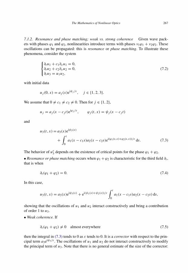
The Mathematics of Nonlinear Optics 267
7.1.2. Resonance and phase matching; weak vs. strong coherence Given wave pack-ets with phases ϕ1 and ϕ2, nonlinearities introduce terms with phases ν1ϕ1 + ν2ϕ2. Theseoscillations can be propagated: this is resonance or phase matching. To illustrate thesephenomena, consider the system∂t u1 + c1∂x u1 = 0,
∂t u2 + c2∂x u2 = 0,∂t u3 = u1u2,
(7.2)
with initial data
u j (0, x) = a j (x)eiψ j /ε, j ∈ {1, 2, 3}.
We assume that 0 6= c1 6= c2 6= 0. Then for j ∈ {1, 2},
u j = a j (x − c j t)eiϕ j /ε, ϕ j (t, x) = ψ j (x − c j t)
and
u3(t, x)= a3(x)eiψ3(x)
+
∫ t
0a1(x − c1s)a2(x − c2s)ei(ϕ1(s,x)+ϕ2(s,x))/ε ds. (7.3)
The behavior of uε3 depends on the existence of critical points for the phase ϕ1 + ϕ2.
• Resonance or phase matching occurs when ϕ1+ϕ2 is characteristic for the third field ∂t ,that is when
∂t (ϕ1 + ϕ2) = 0. (7.4)
In this case,
u3(t, x) = a3(x)eiψ3(x) + ei(ψ1(x)+ψ2(x))/ε∫ t
0a1(x − c1s)a2(x − c2s) ds,
showing that the oscillations of u1 and u2 interact constructively and bring a contributionof order 1 to u3.
• Weak coherence. If
∂t (ϕ1 + ϕ2) 6= 0 almost everywhere (7.5)
then the integral in (7.3) tends to 0 as ε tends to 0. It is a corrector with respect to the prin-cipal term a3eiψ3/ε. The oscillations of u1 and u2 do not interact constructively to modifythe principal term of u3. Note that there is no general estimate of the size of the corrector:

268 G. Metivier
it is O(√ε) if the phase has only non-degenerate critical points, it is O(ε1/p) when there
are degenerate critical points of finite order.
• Strong coherence. Suppose that
∂t (ϕ1 + ϕ2) 6= 0 everywhere. (7.6)
In this case, and in this case only, one can perform direct integration by parts of the integraland the corrector is O(ε). Indeed, if the coefficients a are smooth, repeated integration byparts yields a complete asymptotic expansion in powers of ε.
CONCLUSION 7.1. Complete asymptotic expansion in powers of ε can exist only if all thephases in play are either resonant or strongly coherent. Otherwise, the convergence to zeroof correctors can be arbitrarily slow.
REMARK 7.2. Resonance is a rare phenomenon. In the example, the phases ϕ1 and ϕ2satisfy
(∂t + c1∂x )ϕ1 = 0, (∂t + c2∂x )ϕ2 = 0, ∂t (ϕ1 + ϕ2) = 0.
Thus
0 = (∂t + c2∂x )∂t (ϕ1 + ϕ2) = ∂t (∂t + c2∂x )ϕ1 = c1(c1 − c2)ψ′′
1 (y − c1t),
implying thatψ ′′1 = 0. Thusψ1 must be a plane phase and ϕ1 = α1(x−c1t)+β1 and, simi-larly, ϕ2 = α2(x−c2t)+β2. The resonance occurs if and only if α1c1+α2c2 = 0, showingthat not only must the phases be planar but also the coefficients must be suitably chosen.
7.1.3. Strong coherence and small divisors Consider initial data for (7.2) which are pe-riodic in y/ε. Thus, for j = 1, 2:
u j (0, x) =∑
na j,n(x)einx/ε, u j (t, x) =
(∑n
a j,n(x − c j t)
)einϕ j /ε
with ϕ j = x − c j t . Suppose that u3(0, x) = 0. Then u3 is the sum of integrals
Im,n =
(∫ t
0a1,m(x − c1s)a2,n(x − c2s)e−i(mc1+nc2)s/ε ds
)ei(m+n)x/ε.
Resonances occur when (m, n) ∈ Z2 are such that
mc1 + nc2 = 0. (7.7)
This shows that the presence of resonances also depends on arithmetical conditions. Forinstance, if c1/c2 6∈ Q, there will be no resonant interaction.
Since ∂t (mϕ1+nϕ2) is a constant, the phases mϕ1+nϕ2 are either resonant or stronglycoherent, yielding integrals which are either O(1) or O(ε). More precisely, in the nonres-

The Mathematics of Nonlinear Optics 269
onant case
Im,n = εO(1)
mc1 + nc2.
However, the convergence of the series∑
Im,n depends on the smallness of the denomina-tors mc1 + nc2.
CONCLUSION 7.3. Interaction phenomena also depend on the arithmetic properties ofthe spectrum of the oscillations. Moreover, the behavior of correctors may also involveproblems of small divisors.
7.1.4. Periodic initial data may lead to almost periodic solutions Consider the followingdispersive system
∂t u1 + ∂x u1 +
1ε
u2 = 0,
∂t u2 − ∂x u2 −1ε
u1 = 0.(7.8)
The phenomenon which we describe below also occurs for non-dispersive system, but indimension d ≥ 2. Consider initial data with a planar phase
u j (0, x) =∑
a j,neinx/ε. (7.9)
The solution reads(u1u2
)=
∑nαn
(i
n + ωn
)ei(ny+ωn t)/ε
+ βn
(n + ωn
i
)ei(ny−ωn t)/ε, (7.10)
with ωn =√
n2 + 1. This solution is periodic in y/ε. However, the set {ωn}n∈Z of timefrequencies is not contained in a finitely generated Z-module. The solution is not periodicin time, it is only almost periodic.
CONCLUSION 7.4. Even for periodic initial data, the solution cannot always be writtenin the form (7.1) u(x,8(x)/ε) with a finite number of phases 81, . . . , 8m and periodicprofiles u(x, θ). The introduction of almost periodic functions can be compulsory.
7.1.5. A single initial phase can generate a space of phases of infinite dimension over RConsider (7.8) with initial data
u j (0, x) =∑
a j,neinx2/ε. (7.11)

270 G. Metivier
We have simply replaced the planar phases nx by the curved phases ψn(x) = nx2/2. Theoutgoing phases are the solutions of the eikonal equation
∂tϕ±n = ±
√1+ (∂yϕ
±n )
2, ϕ±n (0, y) = ψn(y).
All the phases ϕ±n are defined and smooth on� = {(t, x); x > |t |, |t | < 1}. One can checkthat the phases ϕn are independent, not only over Q, but also over R.
CONCLUSION 7.5. A one dimensional vector space of initial phases can generate a spaceof phases of infinite dimension over R. In this case, any description (7.1) must include aninfinite number of phases, whatever the properties imposed on the spectrum of the profiles.
7.1.6. Multidimensional effects We have already discussed the effects of focusing inSection 5.4: the linear amplification can be augmented by a nonlinear term and produceblow up. We briefly discuss below two other examples taken from [76].
A more dramatic multidimensional effect is instantaneous blow up, which may occurwhen the initial phase ϕ has a stationary point. This is illustrated in the following example.Consider in dimension d = 3{
(∂2t −1x )u
ε= 0, uε
|t=0 = 0, ∂t uε|t=0 = h(|x |2)ei|x |2/ε,
∂tvε= |∂t u
ε|2|vε|2, vε
|t=0 = v0(x).(7.12)
Then
uε(t, 0) = th(t)eit2/ε ∂t uε= 2iε−1t2h(t)eit2/ε
+ O(1).
Therefore, if h(0) = 1, |∂t uε| ≥ ε−1t2 in an interval [0, T0] and if v0(0) = 1,
v(t, 0) ≥1
1− t5/5ε2 .
This proves that the maximal time of existence of bounded solutions is T (ε) . ε25 , and
there is no uniform domain of existence of solutions.When combined with phase interaction, the focusing effects can come from linear com-
binations of the phases, before the initial phase focus. More precisely, the initial data canlaunch regular phases ϕ j ; nonlinear interaction creates new phases ψ =
∑n jϕ j , and one
among them may have a critical point at t = 0, producing instantaneous explosion. Thisphenomenon is called hidden focusing in [76] and is illustrated by the following example
(∂2t −1x )u
ε= 0, uε
|t=0 = 0, ∂t uε|t=0 = eix1/ε,
(∂2t − c1x )v
ε+ a∂1v
ε= 0, vε
|t=0 = εeix1/ε, ∂t u
ε|t=0 = b(0, x)eix1/ε,
(∂2t − 31x )w
ε= f ε, uε
|t=0 = 0, ∂t uε|t=0 = eix1/ε,
∂t zε= |∂x1w
ε|2|zε|2, vε
|t=0 = 0,

The Mathematics of Nonlinear Optics 271
with
f ε =1
(b(t, x))2(∂t uε + ∂x1uε
)3 (∂t u
ε− ∂x1uε
)(∂tv
ε)2.
The phases in play are ϕ1 = x − t , ϕ2 = x + t and the solutions ϕ3 and ϕ4 of the eikonalequation for ∂2
t − c1x with initial value x1. If c(0, 0) = 2, ϕ3 = x + 2t + 0(t2+ |t x |) and
ϕ4 = x − 2t + 0(t2+ |t x |). In particular, the phase φ = −2ϕ2+ϕ1+ 2ϕ3 = O(t2
+ |t x |),which is revealed by the interaction f ε, has a critical point at the origin, producing blowup in the fourth equation as in the previous example:
PROPOSITION 7.6 ([76]). One can choose the functions a(t, x), b(t, x) and c(t, x) such
that c(0, 0) = 2 and the maximal time of existence of bounded solutions is T (ε) . ε16 .
7.2. Description of oscillations
In this section we deviate slightly from the central objective of nonlinear optics, and evokethe more general question of how one can model oscillations.
7.2.1. Group of phases, group of frequencies In the representation (7.1), 8 is thoughtof as a vector-valued function of (t, x), for instance 8 = (ϕ1, . . . , ϕm), and the phases arelinear combinations ϕ =
∑α jϕ j = α ·8; the important property of the set of α is that it
must be an additive group, to account for wave interaction. As explained in the examplesabove, this group is not necessarily finitely generated, for instance in the case of almostperiodic oscillations. This leads to the following framework:
ASSUMPTION 7.7. 3 is an Abelian group (called the group of frequencies) and we havean injective homomorphism from 3 to C∞(�;R) where � is an open set in R1+d . Wedenote it by α 7→ α ·8.
The set F = 3 ·8 is an additive subgroup of C∞(�;R) (the group of phases) assumedto contain no nonzero constant function.
We also assume that for all ϕ ∈ F \ {0}, dϕ 6= 0 a.e. in �.
We denote by α · 8(t, x) the value at (t, x) of the phase α · 8, and by α · d8(t, x)its differential. The notation α 7→ α · 8 for the homomorphism from 3 7→ C∞(�;R) ischosen to mimic the case where 3 ⊂ Rm and 8 ∈ C∞(�;Rm).
EXAMPLES 7.8. (a) When F is finitely generated, one can choose a basis over Z andwe are reduced to the case where 3 = Zp.
(b) Another interesting case occurs when the R-vector space generated by F , called F ,is of finite dimension m over R. Then one can choose a finite basis (ψ`) of F anddenote by ·9 the mapping β ·9 =
∑1≤`≤m β`ψ
k from Rm to F . Then, we have agroup homomorphism M : 3 7→ Rm such that
α ·8 = (Mα) ·9. (7.13)
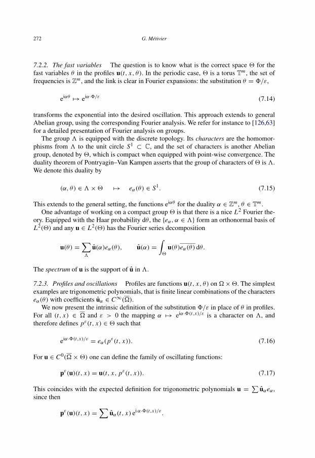
272 G. Metivier
7.2.2. The fast variables The question is to know what is the correct space 2 for thefast variables θ in the profiles u(t, x, θ). In the periodic case, 2 is a torus Tm , the set offrequencies is Zm , and the link is clear in Fourier expansions: the substitution θ = 8/ε,
eiαθ7→ eiα·8/ε (7.14)
transforms the exponential into the desired oscillation. This approach extends to generalAbelian group, using the corresponding Fourier analysis. We refer for instance to [126,63]for a detailed presentation of Fourier analysis on groups.
The group 3 is equipped with the discrete topology. Its characters are the homomor-phisms from 3 to the unit circle S1
⊂ C, and the set of characters is another Abeliangroup, denoted by 2, which is compact when equipped with point-wise convergence. Theduality theorem of Pontryagin–Van Kampen asserts that the group of characters of2 is3.We denote this duality by
(α, θ) ∈ 3×2 7→ eα(θ) ∈ S1. (7.15)
This extends to the general setting, the functions eiαθ for the duality α ∈ Zm , θ ∈ Tm .One advantage of working on a compact group 2 is that there is a nice L2 Fourier the-
ory. Equipped with the Haar probability dθ , the {eα, α ∈ 3} form an orthonormal basis ofL2(2) and any u ∈ L2(2) has the Fourier series decomposition
u(θ) =∑3
u(α)eα(θ), u(α) =∫2
u(θ)eα(θ) dθ.
The spectrum of u is the support of u in 3.
7.2.3. Profiles and oscillations Profiles are functions u(t, x, θ) on �×2. The simplestexamples are trigonometric polynomials, that is finite linear combinations of the characterseα(θ) with coefficients uα ∈ C∞(�).
We now present the intrinsic definition of the substitution 8/ε in place of θ in profiles.For all (t, x) ∈ � and ε > 0 the mapping α 7→ eiα·8(t,x)/ε is a character on 3, andtherefore defines pε(t, x) ∈ 2 such that
eiα·8(t,x)/ε= eα(p
ε(t, x)). (7.16)
For u ∈ C0(�×2) one can define the family of oscillating functions:
pε(u)(t, x) = u(t, x, pε(t, x)). (7.17)
This coincides with the expected definition for trigonometric polynomials u =∑
uαeα ,since then
pε(u)(t, x) =∑
uα(t, x) eiα·8(t,x)/ε.

The Mathematics of Nonlinear Optics 273
7.2.4. Profiles in L p and associated oscillating families The definition of the substitu-tion can be extended to profiles u ∈ L p, p < +∞, not for a fixed ε, but in an asymptoticway. The result is a class of bounded families in L p, modulo families which convergestrongly to 0. The key observation is the following:
PROPOSITION 7.9. For u ∈ C00(�×2) and 1 ≤ p < +∞, there holds
‖u‖L p(�×2) = limε→0‖pε(u)‖L p(�).
PROOF. v = |u |p ∈ C00(�×2) and it is sufficient to prove that∫
�×2
v(t, x, θ) dtdxdθ = limε→0
∫�
pε(v)(t, x) dtdx .
By density one can assume that v is a trigonometric polynomial. In this case∫�
pε(u)(t, x) dtdx =∫�
∑u(t, x, α) eiα·8(t,x)/ε dtdx
−−→ε→0
∫�
u(t, x, 0) dtdx =∫�×2
u(t, x, θ) dtdxdθ
where the convergence follows from Lebesgue’s lemma and the assumption that d(α ·8) 6=0, a.e. if α 6= 0. �
DEFINITION 7.10. Let L pε (�) denote the space of families (uε) which are bounded in
L p(�). Two families (uε) and (vε) are equivalent if (uε − vε) tends to 0 in L p(�). This isdenoted by (uε) ∼ (vε).
Consider the following semi-norm on L pε (�):
‖(uε)‖p = lim supε→0
‖uε‖L p(�). (7.18)
The set N pε of families (uε) such that ‖(uε)‖p = 0 is the subspace of families (uε) ∼ 0
which converge strongly to zero in L p(�). The quotient space L pε /N p
ε is a space ofbounded families in L p modulo families which converge strongly to 0. With the norm(7.18) it is a Banach space.
For u ∈ C00(� ×2) the family (uε) = (pε(u)) is bounded in L p(�). Seen in the quo-
tient space L pε , Proposition 7.9 implies that pε defined on C0
0(� × 2) is an isometry forthe norms of L p(�×2) and L p
ε (�). Thus by density, pε extends as an isometry pε fromL p(�×2) into L p
ε .
DEFINITION 7.11 (F -oscillating families in L p). L pε,F denotes the image of L p(�×2)
by pε. A family (uε) in L pε is called F -oscillating, if its image in the quotient L p
ε belongsto L p
ε,F . The space of such families is denoted bu L pε,F ⊂ L p
ε .

274 G. Metivier
Because pε is an isometry, for (uε) ∈ L pε,F , there is a unique u ∈ L p(�×2) such that
(uε) ∈ pε(u). This u is called the profile of the oscillating family (uε) and we can think ofit as
uε(t, x) ∼ u(t, x, pε(t, x))
where the ∼ is taken in the sense that the difference converges to 0 in L p, the substitutionis exact if u is continuous, and taken in the extended sense if u ∈ L p.
7.2.5. Multi-scale weak convergence, weak profiles
PROPOSITION 7.12. If 3 is countable, then for all (uε) ∈ L pε (�), 1 < p < +∞, there is
a sequence εn → 0 and also u ∈ L p(�×2), such that for all trigonometric polynomials a:∫�
uεn (t, x)pεn (a)(t, x)dtdx −−−→εn→0
∫�×2
u(t, x, θ) a(t, x, θ) dtdx dθ. (7.19)
This u is called the weak profile with respect to the group of phases F of the family (uεn ).In other contexts it is also called the two-scale weak limit.
If (uε) ∈ L pε,F is F oscillating with profile u, then u is also the weak profile of the
family and no extraction of subsequence is necessary.We do not investigate these notions further. They have been used in the context of geo-
metric optics in [79,80], see also Section 7.6.4 below. They are also useful in other situa-tions such as homogeneisation.
7.3. Formal multi-phases expansions
The goal of this section is to show that the formal analysis of Section 5.2 can be carried outin the more general setting of multi-phase expansions. We consider the weakly nonlinearframework, that is equations of the form
A0(a, εu)∂t u +d∑
j=1
A j (a, εu)∂x j u +1ε
E(a)u = F(u) (7.20)
where the coefficient a = a(t, x) is smooth and given. The matrices A j and E are as-sumed to be smooth functions of their arguments. Moreover, the A j are self-adjoint withA0 positive definite and E is skew-adjoint. The source term F is a smooth function of itsarguments.
7.3.1. Phases and profiles. Weak coherence Following the general principles, we con-sider a group of phases F and also introduce the vector space F they span. The character-

The Mathematics of Nonlinear Optics 275
istic phases play a prominent role. We use the notations
{A j (a) = A j (a, 0),L(a, ∂) = A0(a)∂t +
∑A j (a)∂x j + E(a) = L1(a, ∂)+ E(a).
(7.21)
ASSUMPTION 7.13 (Weak coherence). We are given an additive subgroup F ofC∞(�;R) such that the vector space F generated by F is finite dimensional over R. Weassume that
(i) for all ϕ ∈ F , either det L(a(t, x), idϕ(t, x)) vanishes everywhere on � and thedimension ker L(a(t, x), idϕ(t, x)) is independent of (t, x), or the determinantdet L(a(t, x), idϕ(t, x)) is different from zero almost everywhere.
(ii) for all ϕ ∈ F \ {0}, dϕ(t, x) 6= 0 for almost all (t, x) ∈ �.
This condition is called weak coherence. The condition (i) means that either ϕ is a char-acteristic phase of constant multiplicity in the sense of Definitions 5.3, or it is characteristicalmost nowhere. For the model (7.2), and F generated by the phases ϕ1 and ϕ2, weak co-herence occurs when α∂tϕ1 + α2∂tϕ2 6= 0 almost everywhere when (α1, α2) 6= (0, 0). Wealso refer to Section 7.6.1 for generic examples in dimension d = 1.
In dimension d > 1, an example (which is indeed strongly coherent as explained below)is the case where a = a is constant and F is a group of planar phases {β0t +
∑β j x j , β ∈
3 ⊂ R1+d}.
Taking a basis (ψ1, . . . , ψm) for F , then any phase ϕ ∈ F is represented as ϕ =β · 9 =
∑β jψ j with β ∈ Rm . The subgroup F corresponds to frequencies β in a sub-
group 3 ⊂ Rm . There are three possibilities:
• The group F (or3) is finitely generated of rank p = m. Then one can choose a basis of Fover Z which is also a basis of F over R. Then the oscillations are naturally represented as
uε(t, x) = u(t, x, 9(t, x)/ε), (7.22)
with u(t, x, θ) 2π periodic in (θ1, . . . , θm). The space for the variables θ is Tm=
(R/2πZ)m .
• The group F is finitely generated of rank p > m. Then one can choose a basis(ϕ1, . . . , ϕp) of F such that F = {α · 8 =
∑α jϕ j ;α ∈ Zp
}. Writing the ϕ j in thebase (ψ1, . . . , ψm) yields a m × p matrix M as in (7.13), such that
3 = MZp, 8(t, x) = t M9(t, x). (7.23)
The oscillations can be represented in two forms:
uε(t, x) = u(t, x, 9(t, x)/ε), (7.24)
uε(t, x) = v(t, x,8(t, x)/ε), (7.25)

276 G. Metivier
with u(t, x, Y ) quasi-periodic in Y with its spectrum contained in 3, or with v(t, x, θ)periodic in (θ1, . . . , θp). In accordance with (7.23), the link between u and v is that
u(t, x, Y ) = v(t, x, t MY ). (7.26)
Identifying periodic functions with functions on the torus, the variables θ can be seen asliving in 2 = Tp.
• The group F is not finitely generated. Then the representation (7.22) involve profilesu(t, x, Y ) which are almost periodic in Y ∈ Rm . Recall that the space of almost periodicfunctions of Y , with values in a Banach space B, is the closure in L∞(Rm
; B) of the set offinite sums
∑eiβY bβ , with β ∈ Rm and bβ ∈ B, called trigonometric polynomials.
The analogue of (7.25) involves a Bohr compactification of Rm (see e.g. [63,126]). Thedual group of the discrete group, 3, is a compact group 2 (see Section 7.2.2). There isa natural mapping π : Rm
7→ 2 defined as follows. A point Y ∈ Rm is mapped to thecharacter α 7→ eiα·Y . In the quasi-periodic case, π = $ ◦ t M , where $ is the natural mapfrom Rp to Tp. The link between almost periodic profiles with spectra contained in 3 andfunctions on the group 2 is that
u(t, x, Y ) = v(t, x, πY ). (7.27)
Similarly, the mapping pε in (7.16) is pε = π(9/ε). In this setting, the oscillations can bewritten
uε(t, x) = v(t, x, π(8(t, x)/ε)), (7.28)
with v(t, x, θ) defined on �×2.
7.3.2. Phases and profiles for the Cauchy problem We make the elementary but impor-tant remark that giving initial oscillating data for the solution uε is not the same as givinginitial data for the profile u, since taking t = 0 in (7.22) yields:
uε(0, x) = u(0, x, 9(0, x)/ε). (7.29)
Given initial oscillations
uε(0, x) = hε(x) ∼ h(x, 90(x)/ε) (7.30)
we have to make the links between 90 and 9 and between u and h which do not dependon the same set of fast variables. The situation is that we have a group F for the phases in� and a group F0 of initial phases. Clearly, the first relation is that F0 = {ϕ|t=0;ϕ ∈ F}.But this is not sufficient: we also want to show that for all ϕ0 ∈ F0 the solutions of theeikonal equation with initial value ϕ0 belong to F . This is a very strong assumption indeed.It is satisfied for instance in the framework of planar phases and also in other interestingcircumstances. The conditions can be summarized in the following assumption:

The Mathematics of Nonlinear Optics 277
ASSUMPTION 7.14 (Weak coherence for the Cauchy problem). Let F = 3 · 9 ⊂ F ⊂C∞(�;R) satisfy Assumption 7.13. We denote by C3 the set of frequencies α ∈ 3 suchthat det L(a, idα ·9) = 0. When α 6∈ C3 let Pα = 0 and when α ∈ C3 let Pα(t, x) denotethe spectral projector of
A−10 (a)
(d∑
j=1
i∂x j (α ·9)A j (a)+ E(a)
)
associated with the eigenvalue −i∂t (α ·9).With ω = � ∩ {t = 0} let F0 ⊂ F0 ⊂ C∞(ω) be the group and vector space of the
restrictions to t = 0 of the phases ϕ in F and F , respectively. We assume that for allϕ0 ∈ F0, dϕ0 6= 0 almost every where on ω.
F0 is finite dimensional, of dimension m0 ≤ m; choosing a basis, defines 90 ∈
C∞(ω;Rm0) and a group 30 ⊂ Rm0 such that F0 = 30 ·90.The mapping ϕ 7→ ϕ|t=0 induces a surjective group homomorphism from 3 to 30,
called ρ, such that
α ·9|t=0 = (ρ(α)) ·90. (7.31)
We assume that
∀α0 ∈ 30, ∀x ∈ ω :∑
α∈ρ−1(α0)
Pα(0, x) = Id . (7.32)
Note that the sum in (7.32) has at most N terms different from zero, since different α’sin ρ−1(α0) correspond to different eigenvalues of A−1
0
(∑i∂x j (α0 ·90)A j + E
). That the
sum is equal to the identity means that all the eigenvalues are present in the sum and thuscorrespond to a characteristic phase α ·9 ∈ F with initial value α0 ·90.
LEMMA 7.15. For a trigonometric polynomial h(x, Y0) =∑
hα0(x)eiα0·Y0 , define
u(0, x, Y ) =∑
Pα(0, x )hρ(α)(x)eiα·Y . (7.33)
Then
u(0, x, 9(0, x)/ε) = h(x, 90(x)/ε). (7.34)
We note that (7.33) also defines a trigonometric polynomial, since there are finitelymany α such that Pα 6= 0 and ρ(α) belongs to the spectrum of h. The identity (7.34) is animmediate consequence of (7.31) and (7.32).
This lemma, when extended to more general classes of profiles, will provide the initialdata for u, when the profile h of the initial data is known.
7.3.3. Formal BKW expansions Given a basis (ψ1, . . . , ψm) of F , we look for solutions
uε ∼∑n≥0
εnun(t, x, 9(t, x)/ε) (7.35)
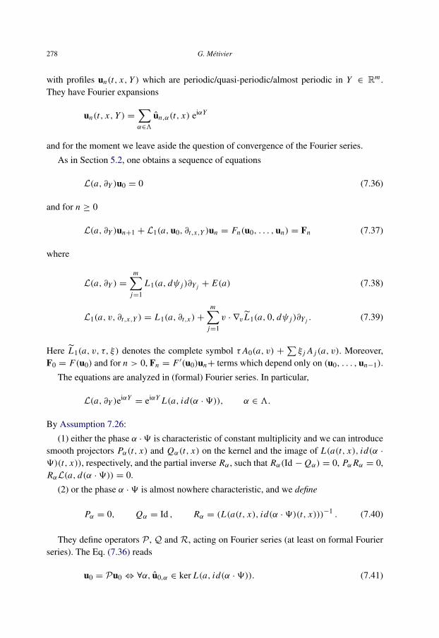
278 G. Metivier
with profiles un(t, x, Y ) which are periodic/quasi-periodic/almost periodic in Y ∈ Rm .They have Fourier expansions
un(t, x, Y ) =∑α∈3
un,α(t, x) eiαY
and for the moment we leave aside the question of convergence of the Fourier series.
As in Section 5.2, one obtains a sequence of equations
L(a, ∂Y )u0 = 0 (7.36)
and for n ≥ 0
L(a, ∂Y )un+1 + L1(a,u0, ∂t,x,Y )un = Fn(u0, . . . ,un) = Fn (7.37)
where
L(a, ∂Y ) =
m∑j=1
L1(a, dψ j )∂Y j + E(a) (7.38)
L1(a, v, ∂t,x,Y ) = L1(a, ∂t,x )+
m∑j=1
v · ∇v L1(a, 0, dψ j )∂Y j . (7.39)
Here L1(a, v, τ, ξ) denotes the complete symbol τ A0(a, v) +∑ξ j A j (a, v). Moreover,
F0 = F(u0) and for n > 0, Fn = F ′(u0)un+ terms which depend only on (u0, . . . ,un−1).
The equations are analyzed in (formal) Fourier series. In particular,
L(a, ∂Y )eiαY= eiαY L(a, id(α ·9)), α ∈ 3.
By Assumption 7.26:
(1) either the phase α ·9 is characteristic of constant multiplicity and we can introducesmooth projectors Pα(t, x) and Qα(t, x) on the kernel and the image of L(a(t, x), id(α ·9)(t, x)), respectively, and the partial inverse Rα , such that Rα(Id −Qα) = 0, PαRα = 0,RαL(a, d(α ·9)) = 0.
(2) or the phase α ·9 is almost nowhere characteristic, and we define
Pα = 0, Qα = Id , Rα = (L(a(t, x), id(α ·9)(t, x)))−1 . (7.40)
They define operators P , Q and R, acting on Fourier series (at least on formal Fourierseries). The Eq. (7.36) reads
u0 = P u0 ⇔ ∀α, u0,α ∈ ker L(a, id(α ·9)). (7.41)

The Mathematics of Nonlinear Optics 279
The Eq. (7.37) is projected by Q and Id −Q; the first part gives
(Id − P)un+1 = R(Fn − L1(a, ∂t,x,Y )un) (7.42)
and the second gives the equation
(Id −Q)(L1(a,u0, ∂t,x,Y )un − Fn) = 0. (7.43)
In particular, the equation for the principal profile is
(Id −Q)L1(a,u0, ∂t,x,Y )P u0 = (Id −Q)F(u0). (7.44)
Knowing u0, (7.42) with n = 0 determines (Id −P)u1; injecting in (7.43) for n = 1 givesan equation for P u1, and so on, by induction.
This is the general scheme at the formal level. To make it rigorous, we have to definethe operators P , Q and R in function spaces and solve the profile equations.
7.3.4. Determination of the main profiles It is important that Eq. (7.44) depends onlyon the definition of the projectors P and Q, and not on the partial inverse R. To fixthe idea, we assume from now on that the projectors Pα(t, x) are the projectors onker L(a(t, x), iα) which are orthogonal for the scalar product induced by A0(a(t, x)),and that Qα = A0(Id − P)A−1
0 = (Id − P∗α ).By the symmetry assumption for L , the projectors Pα and Qα are uniformly bounded in
α. Moreover, smoothess in x for fixed α follows from the constant multiplicity assumption.However, when studying the convergence properties of the Fourier series defining P andQ, we need a little bit more:
ASSUMPTION 7.16 (Uniform coherence). The projectors Pα and Qα are bounded, as wellas their derivatives, uniformly with respect to (t, x) ∈ � and α ∈ 3.
EXAMPLE 7.17. This condition is trivially satisfied if a(t, x) = a is constant, since thenthe projectors are bounded and independent of (t, x). As in Proposition 4.18, it also holdsif the symbol L(a(t, x), η) is symmetric hyperbolic in a direction η with constant multi-plicities in (t, x, η) for η 6= 0.
Several frameworks can be considered:
(H1) The group F is finitely generated of rank p ≥ m.In this case, instead of the quasi-periodic representation (7.22) one uses the periodic one
(7.25). With obvious modifications, the equation reads
(Id −Q)L1(a,u0, ∂t,x,θ )P u0 = (Id −Q)F(u0). (7.45)
The profiles are sought in Sobolev spaces H s(�× Tp). One key argument for the conver-gence of Fourier series is Plancherel’s theorem: for u(x, θ) =
∑uα(x)eiα·θ the following

280 G. Metivier
expression holds
‖u‖2H s (ω×Tp) ≈
∑α
‖uα‖2H s (ω) + |α|2s‖uα‖2L2(ω)
. (7.46)
The profile equation inherits symmetry from the original equation and can be solved by aniterative scheme, in the spirit of the general theory of symmetric hyperbolic systems (seeTheorem 3.2).
(H2) The equation is semi-linear and the nonlinearity F is real analytic.In this case, one can use Wiener’s algebra of almost periodic functions
As=
{u(x, Y ) =
∑uα(x)eiαY
;
∑α
∥∥uα∥∥
H s <∞
}.
The profile equation on Fourier series reads
(Id − Qα)L1(a, ∂t,x )Pαu0,α = (Id − Qα)F0,α, α ∈ 3. (7.47)
For each α, (Id − Qα)L1(a, ∂t,x )Pα is a hyperbolic system (Lemma 5.7). Assuming F0given, or given by an iterative process, the coefficients u0,α can be determined from theirinitial values. Because the projectors are uniformly bounded the equations (7.47) can beuniformly solved. Next, we note that because F is real analytic, it maps the space Es intoitself if s > d
2 .To simplify the exposition we use the following notations and terminology:
NOTATIONS 7.18. � is a truncated cone {(t, x) : 0 ≤ t ≤ T λ∗t + |x | ≤ R} with T ≤ T0and λ∗ will be chosen large enough so that � will be contained in the domain of determi-nacy of ω = {x : |x | ≤ R} whenever this is necessary (see the discussion in Section 3.6).
Recall also from this section, u defined on� is said to be continuous in time with valuesin L2 if its extension by 0 outside� belongs to C0([0, T0]; L2(Rd)); for s ∈ N, we say thatu is continuous with values in H s if the derivatives ∂αx u for |α| ≤ s are continuous in timewith values in L2. We denote these spaces by C0 H s(�).
There are analogous definitions and notations for functions defined on � × Tp or�× Rm .
THEOREM 7.19 (Existence of the principal profile under the uniform weak coherence as-sumption). Suppose that Assumptions 7.13, 7.16 and (H1) [resp. (H2)] are satisfied. Forall initial data P u0|t=0 given in H s(ω×Tp) with s > d+p
2 + 1 [resp. Es(ω) with s > d2 ],
there exists T > 0 such that the profile equations (7.41) (7.44) have a unique solutionu0 ∈ C0 H s ((� ∩ {t ≤ T })× Tp) [resp. C0As(� ∩ {t ≤ T })]
For details, we refer the reader to [74,75].
7.3.5. Main profiles for the Cauchy problem The previous theorem solves the profileequations knowing the value of u0 at time t = 0. When considering the Cauchy problemwith oscillating data (7.30), one has to lift the initial profile h to an initial condition for u0.
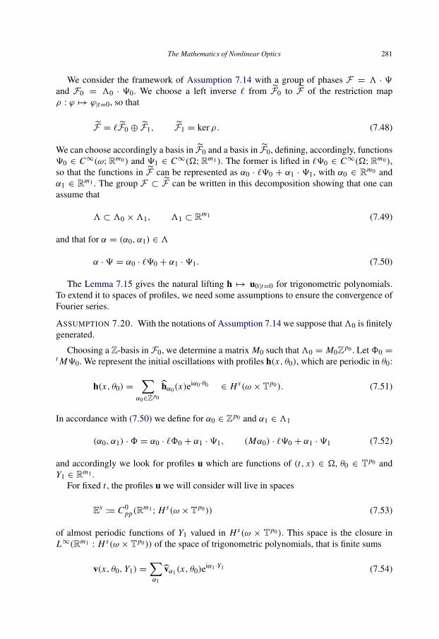
The Mathematics of Nonlinear Optics 281
We consider the framework of Assumption 7.14 with a group of phases F = 3 · 9
and F0 = 30 · 90. We choose a left inverse ` from F0 to F of the restriction mapρ : ϕ 7→ ϕ|t=0, so that
F = `F0 ⊕ F1, F1 = ker ρ. (7.48)
We can choose accordingly a basis in F0 and a basis in F0, defining, accordingly, functions90 ∈ C∞(ω;Rm0) and 91 ∈ C∞(�;Rm1). The former is lifted in `90 ∈ C∞(�;Rm0),so that the functions in F can be represented as α0 · `90 + α1 · 91, with α0 ∈ Rm0 andα1 ∈ Rm1 . The group F ⊂ F can be written in this decomposition showing that one canassume that
3 ⊂ 30 ×31, 31 ⊂ Rm1 (7.49)
and that for α = (α0, α1) ∈ 3
α ·9 = α0 · `90 + α1 ·91. (7.50)
The Lemma 7.15 gives the natural lifting h 7→ u0|t=0 for trigonometric polynomials.To extend it to spaces of profiles, we need some assumptions to ensure the convergence ofFourier series.
ASSUMPTION 7.20. With the notations of Assumption 7.14 we suppose that30 is finitelygenerated.
Choosing a Z-basis in F0, we determine a matrix M0 such that30 = M0Zp0 . Let80 =t M90. We represent the initial oscillations with profiles h(x, θ0), which are periodic in θ0:
h(x, θ0) =∑
α0∈Zp0
hα0(x)eiα0·θ0 ∈ H s(ω × Tp0). (7.51)
In accordance with (7.50) we define for α0 ∈ Zp0 and α1 ∈ 31
(α0, α1) ·8 = α0 · `80 + α1 ·91, (Mα0) · `90 + α1 ·91 (7.52)
and accordingly we look for profiles u which are functions of (t, x) ∈ �, θ0 ∈ Tp0 andY1 ∈ Rm1 .
For fixed t , the profiles u we will consider will live in spaces
Es:= C0
pp(Rm1; H s(ω × Tp0)) (7.53)
of almost periodic functions of Y1 valued in H s(ω × Tp0). This space is the closure inL∞(Rm1 : H s(ω × Tp0)) of the space of trigonometric polynomials, that is finite sums
v(x, θ0, Y1) =∑α1
vα1(x, θ0)eiα1·Y1 (7.54)

282 G. Metivier
with coefficients vα1 ∈ H s(ω×Tp0). Each coefficient can be in its turn expanded in Fourierseries in θ0.
Following the notations of Assumptions 7.14 and 7.20, we denote by C3 the set of(α0, α1) ∈ Zp0 × 31 such that (M0α0, α1) belongs to 3 and the corresponding phase(α0, α1)·8 is characteristic. With little risk of confusion, we denote by P(α0,α1) and Q(α0,α1)
the associated projectors. For (α0, α1) 6∈ C3, we set P(α0,α1) = 0 and Q(α0,α1) = Id .The projectors P and Q are obviously defined on trigonometric polynomials,∑
vα0,α1(x)ei(α0·θ0+α1·Y1).
LEMMA 7.21. The projector P extends as a bounded projector in E0.
PROOF. For a trigonometric polynomial with coefficients vα0,α1 , let w = P v and define
Vα0(x, Y1) =∑α1
vα0,α1(x)eiα1·Y1 ,
Wα0(x, Y1) =∑α1
wα0,α1(x)eiα1·Y1 =
∑α1
P(α0,α1 )vα0,α1(x)eiα1·Y1 .
Because the number of α1 such that (α0, α1) ∈ C3 is at most N and the projectors arebounded, the following holds∣∣Wα0(x, Y1)
∣∣2 ≤ NC∑α1
∣∣vα0,α1(x)∣∣2
= NC limR→∞
1(2R)m1
∫[−R,R]m1
∣∣Vα0(x, Y )∣∣2 dY.
Thus, by Fatou’s lemma,
‖w(·, ·, Y1)‖2L2(ω×Tp0 )
≤ NC limR→∞
1(2R)m1
×
∫[−R,R]m1
‖w(·, ·, Y )‖2L2(ω×Tp0 )dY
≤ NC supY∈Rm1
‖w(·, ·, Y )‖2L2(ω×Tp0 ).
This proves that P is bounded on trigonometric polynomials for the norm of E0. Thelemma follows by density. �
Using Assumption 7.16, one can repeat the proof for derivatives and P acts from Es
to Es . There is a similar proof for the action of Id − Q and thus for Q. Finally, forh ∈ H s(ω × Tp0), one can construct
`h(x, θ0, Y1) =∑α0,α1
P(α0,α1 )hα0(x)ei(θ0·θ0+α1·Y1) ∈ Es (7.55)

The Mathematics of Nonlinear Optics 283
using again the fact that for each α0 there are at most N non-vanishing terms in the sum.Therefore:
PROPOSITION 7.22. Under Assumptions 7.14, 7.16 and 7.20, the projectors P and Qare well defined in the spaces Es for all s ≥ 0. In addition, the lifting operator (7.55) isbounded from H∞(ω × Tp0) into Es and (Id − P)` = 0.
Using the Notations 7.18, we can repeat
THEOREM 7.23 (Existence of the principal profile for the Cauchy problem under the uni-form weak coherence assumption). Suppose that Assumptions 7.14, 7.16 and 7.20 aresatisfied. For all data h ∈ H s(ω×Tp0) with s > d+p
2 +1, there exists T > 0 such that theprofile equations (7.41) (7.44) have a unique solution u0 ∈ C0Es (� ∩ {t ≤ T }) satisfying
u0(0, x, θ0, Y1) = `h. (7.56)
This is proved in [76] when 31 = R, but the proof extends immediately to the gen-eral case considered here. It is based on the symmetry property inherited by the profileequation, and the fact that the projectors act in the proper spaces.
7.3.6. Approximate solutions at order o(1) in L2 When u0 is known, to solve the equa-tion with an error O(ε), it would be sufficient to determine u1 such that
L(a, ∂Y )u1 = Q(F0 − L1(a, ∂t,x,Y )u0
), (7.57)
that is, formally,
(Id − P)u1 = R(F0 − L1(a, ∂t,x,Y )u0
). (7.58)
Obviously, the principal difficulty is to show that R is a bounded operator on suitablespaces of profiles. The weak coherence Assumption 7.13 permits phases α · 9 such thatthe determinant det L(a, idα · 9) vanishes on a set of measure 0. In this case the inverseRα = (L(a, idα ·9))−1 is defined almost everywhere but is certainly not bounded. How-ever, this is sufficient to obtain approximate solutions in spaces of low regularity. To givean idea of a possible result consider the Cauchy problem for (7.20) in the framework ofTheorem 7.23.
THEOREM 7.24. Under the assumptions of Theorem 7.23 suppose that h ∈ H s(ω×Tp0)
is given and u0 ∈ C0Es(�) is a solution of the main profile equation with initial data(7.56). Then, there is a family of functions uε ∈ C0L2(�) such that
uε(0, x)− h(x,80(x)/ε)→ 0 in L2(ω),
uε(t, x)− u0(t, x,8(t, x)/ε)→ 0 in C0L2(�)
and
A0(a, εuε)∂t u
ε+
d∑j=1
εA j (a, εuε)∂x j u
ε+
1ε
E(a)uε = F(uε)+ f ε (7.59)

284 G. Metivier
with f ε → 0 in L2(�).
SCHEME OF THE PROOF. Step 1. The profile f0 := F0 − L1(a, ∂t,x,Y )u0 is known andcan be approximated by trigonometric polynomials: for all δ > 0, there is a finite sumf′0 =
∑eiαY fα such that ‖f0 − f′‖ ≤ δ, in the space of profiles.
Step 2. One can modify the Fourier coefficients fα , and assume that they are smooth andvanish near the negligible set where det L(a, dα ·9) vanishes. One can then ensure that∥∥(f0 − f′0)( ·,8(·)/ε)
∥∥L2(�)
≤ 2δ. (7.60)
Step 3. The conditions on fα allow one to define Rα fα and therefore an approximate firstcorrector u′1 which is a smooth trigonometric polynomial.
Consider uε(t, x) = (u0 + εu′1)(t, x,8(t, x)/ε). It satisfies∣∣uε(t, x)− u0(t, x,8(t, x)/ε)∣∣ ≤ εK (δ)
and satisfies the equation up to an error eε(t, x) which is (f0 − f′)(t, x, 9(t, x)/ε) plusterms factored by ε and involving u1 and u0. Thus∥∥eε
∥∥L2 ≤ 2δ + εK (δ).
Choosing δ = δ(ε)→ 0 sufficiently slowly, so that εK (δ)→ 0 proves the theorem. �
REMARK 7.25. Because we truncate the Fourier coefficients in Step 2, estimates of theerror f ε in L2 (or in L p but with p <∞) is the best that one can expect with this method.
7.3.7. Strong coherence The difficulty caused by the phases such that det L(a, idϕ) van-ishes on a small set, is not only a technical difficulty met in the definition of the correctoru1, but the examples of Section 7.1.6 show that this problem can have severe consequences.To avoid them, the following condition is natural:
ASSUMPTION 7.26 (Strong coherence). We are given an additive subgroup F ofC∞(�;R) such that the vector space F generated by F is finite dimensional over R. Weassume that
(i) for all ϕ ∈ F the dimension of the kernel of det L(a(t, x), idϕ(t, x)) is independentof (t, x) ∈ �,
(ii) for all ϕ ∈ F \ {0}, dϕ(t, x) 6= 0 for all (t, x) ∈ �.
EXAMPLE 7.27. An important example is the case where a = a is constant and F is agroup of planar phases {β0t +
∑β j x j , β ∈ 3 ⊂ R1+d
}. We refer to [74,76] for otherexamples and a detailed discussion of this assumption. We just mention here the case ofphases generated by {|x | ± t, t} in the case of the wave equation, or Maxwell equations, ormore generally in the case of spherically invariant systems.
In particular, (i) implies that each phase ϕ ∈ F is either characteristic everywhere ornowhere characteristic. This assumption implies that all the partial inverses Rα are well de-fined everywhere on �. Therefore Step 2 in the proof of Theorem 7.24 can be eliminated.

The Mathematics of Nonlinear Optics 285
REMARK 7.28. When the strong coherence assumption is satisfied, the approximation re-sults in Theorem 7.24 can be improved, so that the errors tend to zero in L∞.
7.3.8. Higher order profiles, approximate solutions at all order Under Assumption 7.26,for each α ∈ 3, the partial inverse Rα(t, x) is well defined everywhere on � and smooth.However, the partial inverses are not necessarily uniformly bounded with respect to α sincethe determinant det L(a, id(α · 9)) can be very small. The summation of the Fourier se-ries for (Id − P)u1 can be delicate and ultimately impossible in certain cases. This is asmall divisors problem which seems difficult to solve in the general framework of almostperiodic profiles.
ASSUMPTION 7.29 (Small divisors conditions). Suppose that Assumption 7.26 is satisfiedand that F is finitely generated. Taking a basis (ϕ1, . . . , ϕp), and representing 3 = MZp
as in (7.23), we assume that for all β ∈ N1+d there are constants c > 0 and ν such that forall α ∈ Zd and for all (t, x) ∈ �:∣∣∣∂βt,x RMα(t, x)
∣∣∣ ≤ C(1+ |α|)ν . (7.61)
EXAMPLE 7.30. When a(t, x) = a is constant and the phases are planar, the matricesRMα are independent of (t, x). The condition (7.61) splits into two conditions: there are cand ν such that, when Mα ·9 is not characteristic∣∣det L(a, id(Mα ·9))
∣∣ ≥ c(1+ |α|)−ν, (7.62)
and when Mα ·9 is characteristic, the nonvanishing eigenvalues λ(α) of L(a, id(Mα ·9))satisfy
|λ(α)| ≥ c(1+ |α|)−ν . (7.63)
Under Assumption 7.29, for F ∈ H∞(�×Tp) the Fourier series defining RF convergesand its sum belongs to F ∈ H∞(�× Tp). This immediately implies the following:
PROPOSITION 7.31. Suppose that Assumption 7.29 is satisfied. If the u0 ∈ H∞(�× Tp)
is given, there is u1 ∈ H∞(�× Tp) satisfying (7.57).
All the ingredients being now prepared, one can construct BKW solutions with arbitrarysmall residuals.
THEOREM 7.32 (Complete asymptotic solution, in the uniformly strongly coherent case,with the small divisors condition). Suppose that � ⊂ [0, T0] × Rd is contained in thedomain of determinacy of the initial domain ω. Suppose that Assumptions 7.16, 7.26 and7.29 are satisfied. Given initial data for P un |t=0 in H∞(ω × Tp) there exists T > 0 anda sequence of profiles un ∈ H∞ ((� ∩ {t ≤ T })× Tp) which satisfy (7.36) (7.37).
We refer to [74] for details. In this paper it is also proved that the small divisor condi-tion is generically satisfied. For instance, for a constant coefficient system, the condition issatisfied for almost all choices of p characteristic planar phases.

286 G. Metivier
Whence one has a BKW solution at all orders, so one can construct approximate solu-tions
uεapp,n(t, x) =n∑
k=0
εnuk(t, x,8(t, x)/ε) (7.64)
which are solutions of the equation with error terms of order O(εn). Using Borel’s Theo-rem, one can construct approximate solutions at infinite orders.
7.4. Exact oscillating solutions
In this section we briefly describe several methods which aim to construct exact solutionsof (7.20) such that
uε(t, x)− u0(t, x, 9(t, x))/ε→ 0 as ε→ 0 (7.65)
where u0 is a principal profile.
7.4.1. Oscillating solutions with complete expansions The easiest case is when onehas a BKW solution at all orders, that is under Assumption 7.29. In this case, one canconstruct approximate solutions uεapp,n(t, x) as in (7.64). Then one can write the equationfor uε − uεapp,n , and if n is large enough, one can use Theorem 4.21 and obtain a resultanalogous to Theorem 5.33. We refer to [74] for details.
7.4.2. Prepared data, continuation of solutions We consider oscillations belonging to afinitely generated group of phases F which satisfies Assumption 7.26. We look for exactsolutions of a non-dispersive equation (7.20) (with E = 0) of the form:
uε(t, x) = uε(t, x,8(t, x)/ε) (7.66)
with uε(t, x, θ) periodic in θ , and 8 related to 9 as in (7.23). For uε to solve (7.20) it issufficient that uε solves
L1(a, εuε, ∂t,x )uε +1ε
L(a, εuε, ∂θ )uε = F(uε) (7.67)
with
L1(a, v, ∂t,x ) = A0(a, v)∂t +
d∑j=1
A j (a, v)∂x j , (7.68)
L(a, v, ∂θ ) =p∑
j=1
L1(a, v, dϕ j )∂θ j . (7.69)

The Mathematics of Nonlinear Optics 287
This is precisely the type of equation (4.35) of (4.45) discussed in Section 4.1.
REMARK 7.33. It is remarkable that the condition (4.39) for (7.69), which is that the rankof L(a(t, x), dα ·8) is constant, is exactly condition (i) of Assumption 7.26. This indicatesthat the conditions of Section 4.1.3, which came from commutation requirements, are notonly technical but deeply related to the focusing effects.
In order to apply Propositions 4.18 and 4.20, we are led to supplement Assumption 7.26with the following
ASSUMPTION 7.34. Assume that there is ψ ∈ F , such that the system L(a, ∂) is hyper-bolic in the direction dψ .
The next result follows directly from Proposition 4.20:
LEMMA 7.35. Under Assumptions 7.26, 7.16 and 7.34, the singular term L(a(t, x), 0, ∂θ )satisfies the Assumption 4.12.
Therefore Theorem 4.14 applies to the Cauchy problem for (7.67) with initial data
uε |t=0(x, θ) = gε(x, θ) (7.70)
(see Remark 4.15). In this context, we have to assume that the data are prepared in thesense of Section 4.1.2, meaning that the times derivatives ∂k
t uε |t=0 which can be computedfrom the equation satisfy
supε∈ ]0,ε0]
∥∥∥∂kt uε |t=0
∥∥∥H s−k (ω×Tp)
<∞. (7.71)
THEOREM 7.36. Suppose that � ⊂ [0, T0] × Rd is contained in the domain of determi-nacy of the initial domain ω. Under Assumptions 7.26 and 7.34, for s > 1 + (d + p)/2and initial data satisfying (7.71), there exists T > 0 such that for ε ∈ ]0, ε0] the Cauchyproblem (7.67) (7.70) has a solution uε in C H s((�∩ {t ≤ T })×Tp), and the family {uε}is bounded in this space.
Moreover, by Theorem 7.19, the Cauchy problem for the principal profile is well-posed.
THEOREM 7.37. Under the assumptions of Theorem 7.36 suppose that in addition, gε →g0 in H s(ω×Tp). Then, uε → u0 in C H s′((�∩ {t ≤ T })×Tp) for all s′ < s, where u0
satisfies the main profile equation with initial data g0.
SKETCH OF PROOF. By compactness, one can extract a subsequence such that uε → u0in C H s′((�∩ {t ≤ T })×Tp) for all s′ < s, implying that u0(0, x, θ) = g0(x, θ). Passingto the limit in the equation (7.67) multiplied by ε, implies that L(a, ∂θ )u0 = 0 and thusthat u0 satisfies the polarization condition P u0 = u0. Next, multiplying the equation by Pkills the singular term, and passing to the limit implies that u0 satisfies the profile equation.By uniqueness of the limit, the full family converges. �

288 G. Metivier
CONCLUSION 7.38. The first theorem means that we have solved the Cauchy problem for(7.20) with initial data
uε |t=0(x) = gε(x,8(0, x)/ε) (7.72)
and found the solution under the form (7.66). The second theorem implies the convergencein (7.65). To apply this method, the difficult part is to check the preparation conditions(7.71). This method is better adapted to continuation problems as in Theorem 4.5 when theoscillations are created, not by the initial data, but by source terms. We leave to the readerto duplicate Theorem 4.5 in the present context.
The assumptions of the theorem are satisfied when a is constant and the phases areplanar; it also applies when the space F is strongly coherent and the system is hyperbolicwith constant multiplicities in the direction dψ of Assumption 7.34 (see Proposition 4.20).
7.4.3. Construction of solutions. General oscillating data Our goal here is to solve theCauchy problem with more general oscillating data, in particular without assuming thepreparation conditions (7.71). The idea is similar to the one developed in the previoussection, but different. We consider initial data of the form
hε(x) = hε(x,80(x)/ε) (7.73)
where hε is a bounded family in H s(ω × Tp0), and we look for solutions of the form
uε(t, x) = uε[(t, x,8[(t, x)/ε) (7.74)
where 8[(0, x) = 80(x). The uε[ are sought in C0 H s(�× Tp0).In this section, we consider a non-dispersive system (7.20) with E = 0. The strategy is
to use Proposition 4.20 and Theorem 4.14, thanks to the following assumption:
ASSUMPTION 7.39. We are given a finitely generated subgroup F[ ⊂ C∞(�) generatinga finite dimensional linear space F[, such that
(i) for all ψ ∈ F[ \ {0} and all (t, x) ∈ �, dxψ(t, x) 6= 0,
(ii) for all ψ ∈ F[ \ {0} A−10 (a(t, x))L(a(t, x), dψ) has eigenvalues independent of
(t, x); moreover, the eigenprojectors belong to a bounded set in C∞(�) indepen-dent of ψ ∈ F .
Choose a R-basis {ψ1, . . . , ψm[} of F[ and a Z-basis {ϕ1, . . . , ϕp[} of F[. Let M[
be the m[ × p[ matrix such that 8[ = t M9[, where 8[ = t (ϕ1, . . . , ϕp[) and 9[ =t (ψ1, . . . , ψm[). We look for solutions of (7.20) of the form (7.74). The equation for uε[reads
L1(a, εuε[, ∂t,x )uε[ +1ε
L[(a, εuε[)uε[ = F(uε[) (7.75)
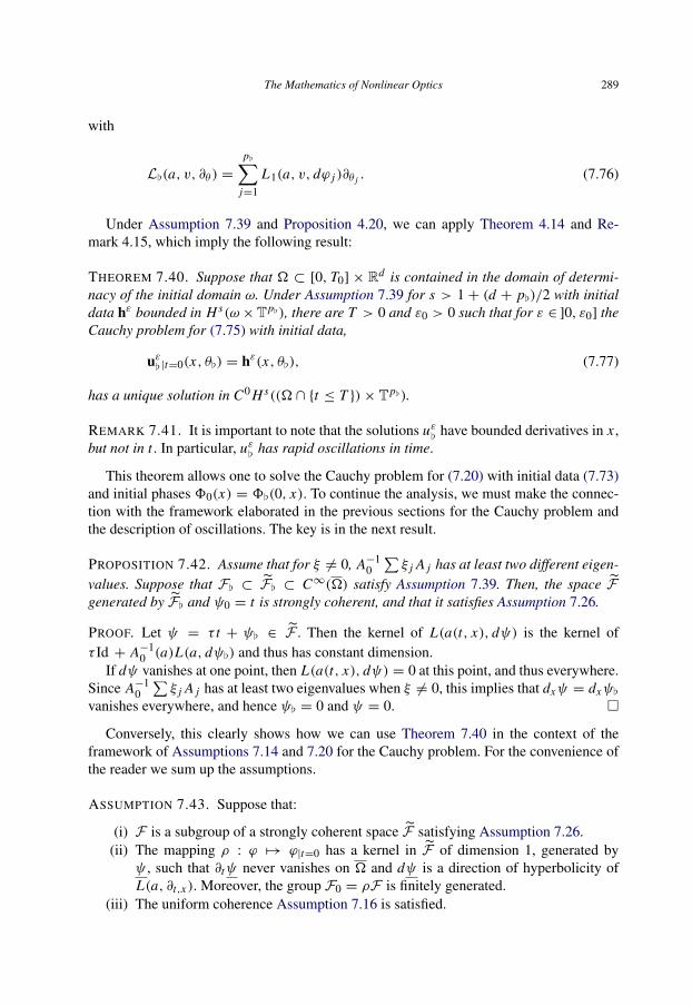
The Mathematics of Nonlinear Optics 289
with
L[(a, v, ∂θ ) =p[∑
j=1
L1(a, v, dϕ j )∂θ j . (7.76)
Under Assumption 7.39 and Proposition 4.20, we can apply Theorem 4.14 and Re-mark 4.15, which imply the following result:
THEOREM 7.40. Suppose that � ⊂ [0, T0] × Rd is contained in the domain of determi-nacy of the initial domain ω. Under Assumption 7.39 for s > 1 + (d + p[)/2 with initialdata hε bounded in H s(ω×Tp[), there are T > 0 and ε0 > 0 such that for ε ∈ ]0, ε0] theCauchy problem for (7.75) with initial data,
uε[ |t=0(x, θ[) = hε(x, θ[), (7.77)
has a unique solution in C0 H s((� ∩ {t ≤ T })× Tp[).
REMARK 7.41. It is important to note that the solutions uε[ have bounded derivatives in x ,but not in t . In particular, uε[ has rapid oscillations in time.
This theorem allows one to solve the Cauchy problem for (7.20) with initial data (7.73)and initial phases 80(x) = 8[(0, x). To continue the analysis, we must make the connec-tion with the framework elaborated in the previous sections for the Cauchy problem andthe description of oscillations. The key is in the next result.
PROPOSITION 7.42. Assume that for ξ 6= 0, A−10
∑ξ j A j has at least two different eigen-
values. Suppose that F[ ⊂ F[ ⊂ C∞(�) satisfy Assumption 7.39. Then, the space Fgenerated by F[ and ψ0 = t is strongly coherent, and that it satisfies Assumption 7.26.
PROOF. Let ψ = τ t + ψ[ ∈ F . Then the kernel of L(a(t, x), dψ) is the kernel ofτ Id + A−1
0 (a)L(a, dψ[) and thus has constant dimension.If dψ vanishes at one point, then L(a(t, x), dψ) = 0 at this point, and thus everywhere.
Since A−10
∑ξ j A j has at least two eigenvalues when ξ 6= 0, this implies that dxψ = dxψ[
vanishes everywhere, and hence ψ[ = 0 and ψ = 0. �
Conversely, this clearly shows how we can use Theorem 7.40 in the context of theframework of Assumptions 7.14 and 7.20 for the Cauchy problem. For the convenience ofthe reader we sum up the assumptions.
ASSUMPTION 7.43. Suppose that:
(i) F is a subgroup of a strongly coherent space F satisfying Assumption 7.26.(ii) The mapping ρ : ϕ 7→ ϕ|t=0 has a kernel in F of dimension 1, generated by
ψ , such that ∂tψ never vanishes on � and dψ is a direction of hyperbolicity ofL(a, ∂t,x ). Moreover, the group F0 = ρF is finitely generated.
(iii) The uniform coherence Assumption 7.16 is satisfied.

290 G. Metivier
With these notations, let F[ be such that F = Rψ ⊕ F[. Let ` be a right inverse of ρ
from F0 = ρF to F[,and let F[ = `F0.
PROPOSITION 7.44. If in addition, possibly after changing the time function, ψ(t, x) = t ,
then F[ ⊂ F[ satisfies Assumption 7.39.
PROOF. If ψ = t , saying that the dimension of the kernel of L(a(t, x), d(τ t + ψ[)) is
constant for all τ , is equivalent to saying that the real eigenvalues of A−10 L(a(t, x), dψ[)
have constant multiplicity. By the hyperbolicity of dψ all the eigenvalues are real. �
REMARK 7.45. In practice, when solving the Cauchy problem with oscillating initial data,one starts with a finitely generated group of phases F0 ⊂ C∞(ω). One constructs all thesolutions of the eikonal equation with initial data in F0, and the group F that they gener-ate. The big constraint is to check that F satisfies Assumption 7.26. The examples givenin Section 7.1 show on one hand that this assumption is very strong, but on the other handthat in the multi-dimensional case direct and hidden focusing effects require such strongconditions.
Under Assumption 7.43 one can solve both the Cauchy problem for data (7.73) by Theo-rem 7.40 and the principal profile equation by Theorem 7.23. Note that the principal profilehere is a function u0(t, x, Y, θ[) with Y ∈ R. Y is the placeholder for ψ/ε = t/ε.
THEOREM 7.46 (Rigorous justification of the geometric optics approximation). Supposethat hε is a bounded family in H s(ω × Tp[) with s > 1 + (d + p[)/2, and that hε → h0
in this space. Let u0 be the solution of the main profile equation given by Theorem 7.23corresponding to h0. Then the Cauchy problem for (7.20) with initial data (7.73) has asolution uε such that
limε→0
supt,x
∣∣uε(t, x)− u0(t, x, t/ε,8[(t, x)/ε)∣∣ = 0. (7.78)
SKETCH OF PROOF (See also [76,117,59,60] and Section 7.5). As in Section 7.3.6, onecan construct uεapp(t, x, θ[) such that
uεapp(t, x, θ[)− u0(t, x, t/ε, θ[)→ 0
in L∞ and uεapp(t, x, θ f lat) is an approximate solution of (7.75) in the sense that is satisfiesthe equation up to an error term which tends to 0 in C0 H s−1(�× Tp[). Then the stabilityproperty of the equation implies that uε[ − uεapp → 0 in C0 H s−1(�× Tp[). �
7.4.4. The case of constant coefficients and planar phases We illustrate the results ofthe previous sections in the important case where a is constant and the phases are planar.We consider here a quasi-linear system
A0(u)∂t u +d∑
j=1
Ax j (u)∂ j u = F(u). (7.79)

The Mathematics of Nonlinear Optics 291
In the regime of weakly nonlinear optics, the solutions are uε = u0 + O(ε) where u0 is asolution with no rapid oscillations. Here we choose u0 to be a constant, which we can taketo be 0, assuming thus that F(0) = 0. We choose planar initial phases and quasi-periodicinitial profiles. We therefore consider initial data of the form
uε |t=0(x) = εhε(x, t M[x/ε) (7.80)
where the hε(x, θ[) are periodic in θ[, bounded in H s(Rd×Tp[), and M[ is a d× p[ matrix.
The initial phases are (M[α) · x for α ∈ Zp[ .Looking for solutions of the form
uε(t, x) = εuε[(t, x, t M[x/ε), (7.81)
yields the equation
A0(εuε[)∂t uε[ +d∑
j=1
A j (εuε[)∂x j uε[ +
1ε
p[∑j=1
B j (εuε[)∂θ j uε[ = G(εuε[)u
ε[ (7.82)
with symmetric matrices B j which we do not compute explicitly here. We are in positionto apply Theorem 4.2:
THEOREM 7.47. With assumptions as above, let {hε; ε ∈ ]0, ε0]} be a bounded fam-ily in H s(Rd
× Tp[) with s > (d + p[ + 1)/2. There exists T > 0 such that forε ∈ ]0, ε0] the Cauchy problem for (7.82) with initial data hε[ has a unique solution
uε[ ∈ C0([0, T ]; H s(Rd× Tp[)).
The profile equation concerns profiles u0(t, x, Y, θ[) periodic in θ[ and almost periodicin Y ∈ R. The profiles satisfy the polarization condition (7.41):
P u0 = u0 (7.83)
and the propagation equation (7.43):
(Id −Q)(L1(∂t , ∂x )u0 + 0(u0, ∂Y , ∂θ[)u0 − G(0)u0
)= 0 (7.84)
where
0(v, ∂Y , ∂θ[)w = v · ∇u A0(0)∂Y w+p[∑
j=1
u∇u B j (0)∂θ j w (7.85)
and the projectors P and Q are defined in Proposition 7.22. In particular, P is the projectoron the kernel of L(∂Y , ∂θ[) = A0(0)∂Y +
∑B j (0)∂θ j . The initial condition for u0 is `h as
in (7.56).

292 G. Metivier
THEOREM 7.48. With assumptions as in Theorem 7.47, suppose that hε → h in H s(Rd×
Tp[). There exists T ′ > 0 such that
(i) the profile equation with initial data `h has a solution u0 ∈ C0([0, T ′];Es) withEs= C0
pp(R; H s(Rd× Tp[));
(ii) and
limε→0
sup0≤t≤min{T,T ′}
∥∥∥uε[(t, ·, ·)− u0(t, ·, t/ε, ·)∥∥∥
H s−1(Rd×Tp[ )= 0. (7.86)
7.5. Asymptotics of exact solutions
In this section we present the principles of different methods which can be used to provethat exact solutions have an asymptotic expansion.
7.5.1. The method of simultaneous approximations The principle of the method. On onehand, there is an equation for exact solutions
∂t uε= Mε(uε, ∂)uε (7.87)
and on the other hand there is another equation for the profiles
∂t u = M(u, ∂)u. (7.88)
The equations are supplemented by initial conditions. The profile u may depend on morevariables than the functions uε. Moreover there is a law u 7→ U ε(u)which assigns a familyof functions to a profile. Both equations are solved by iteration:
∂t uεν+1 = Mε(uεν, ∂)u
εν+1, (7.89)
∂t uν+1 = M(uν, ∂)uν+1. (7.90)
The principle of the method relies on the following elementary lemma:
LEMMA 7.49. Suppose that
(1) the sequence uεν converges to uε, uniformly in ε in a space X;(2) the sequence uν converges to u in a space X ;(3) the mapping u 7→ {U ε(u), ε ∈ ]0, ε0]} maps continuously X to the space of
bounded families in X equipped with the topology of uniform convergence;(4) for the initial term ν = 0 of the induction, uε0 −U ε(u0)→ 0 in X;(5) for each ν ≥ 0, assuming that uεν −U ε(uν)→ 0 in X, then uεν+1−U ε(uν+1)→ 0
in X.
Then uε −U ε(u)→ 0 in X.

The Mathematics of Nonlinear Optics 293
PROOF. By (4) and (5), the property (6), uεν − U ε(uν)→ 0 in X , is true for all ν. By (1)for δ > 0, there is ν0 such that for all ν ≥ ν0 and all ε ∈ ]0, ε0]:
‖uε − uεν‖X ≤ δ.
Moreover, by (2) and (3), for ν large enough, the following holds
‖U ε(u)−U ε(uν)‖X ≤ δ.
Thus, choosing ν such that both properties are satisfied and using (6), we see that
lim supε→0
‖uε −U ε(u)‖X ≤ 2δ
and the lemma follows. �
Of course, this lemma is just a general principle which can (and often must) be adaptedto particular circumstances of the cases under examination.
REMARK 7.50. In this strategy, the main step is the fifth, which amounts to prove that fora linear equation whose coefficients have given asymptotic expansions, the solution has anasymptotic expansion.
Application to the oscillating Cauchy problem. This method has been applied in d = 1with spaces X of C1 functions and spaces of profiles X of class C1 in all the variables andalmost periodic in the fast variables (see [82] and Section 7.6.1 below).
It has been applied also in the multidimensional case d > 1, for coherent almost peri-odic oscillations in the Wiener Algebra and semi-linear equations (see Theorem 7.19 forthe context and [75] for precise results.)
We now briefly review how it is applied to prove the second part of Theorem 7.46 asin [76]. For simplicity, we consider the case of Eq. (7.79) and planar phases as in Theo-rem 7.48. The equations for exact solutions are given in (7.82) and for the profiles in (7.83)(7.84). The iterative scheme leads to linear problems
A0(εvε[)∂t uε[ +d∑
j=1
A j (εvε[)∂x j uε[ +
1ε
p[∑j=1
B j (εvε[)∂θ j uε[ = G(εvε[)v
ε[ (7.91)
and {P u = u(Id −Q)
(L1(∂t , ∂x )u+ 0(v, ∂Y , ∂θ[)u− G(0)v
)= 0.
(7.92)
The key point is to prove that if the vε are bounded in C0[0, T ]; H s(Rd
× Tp[),if u ∈ C0([0, T ],Es(R × Rd
× Tp[)), and if vε[(t, x, θ[) − v(t, x, t/ε, θ[) tends to
0 in C0([0, T ]; H s−1(Rd× Tp[)), then uε[(t, x, θ[) − u(t, x, t/ε, θ[) tends to 0 in
C0([0, T ]; H s−1(Rd×Tp[)). This means that the problem of the asymptotic description of
solutions is completely transformed into linear problems. Using approximations, one can

294 G. Metivier
restrict the analysis to the case where v is a trigonometric polynomial, and in this case wecan use BKW solutions.
7.5.2. The filtering method This method has been introduced in [86,87], with motiva-tion coming from fluid Mechanics, in particular with applications to the analysis of thelow Mach limit of Euler equations. Next it was extended to more general contexts such as(7.82) in [88,115–118], and then adapted to various other problems by many authors.
The principle of the method. The method applies to evolution equations where two timescales (at least) are present:
∂t uε+
1ε
Guε +8(uε) = 0, uε |t=0 = hε (7.93)
where G generates a C0 group e−tG , which is uniformly bounded in a Hilbert space H1,and also uniformly bounded in H ⊂ H1. Moreover, 8 is a bounded family of continuousfunctionals from H to H1 which map bounded sets in H to bounded sets in H1.
It is assumed that there is a preliminary construction which provides us with a family ofsolutions uε bounded in C0([0, T ]; H). The problem is to describe the asymptotic behav-ior of uε. Assume that the embedding H ⊂ H1 is compact and hε → h in H . The problemthen is to describe the fast oscillations in time of uε. The idea is very classical in the studyof evolution systems, and can be related to themes like adiabatic limits or the constructionof wave operators in scattering theory: set
vε(t) = etε
Guε(t)⇔ uε(t) = e−tε
Gvε(t). (7.94)
Thus vε is bounded in C0([0, T ]; H) and
∂tvε(t) = −e
tε
G8ε(uε(t)) (7.95)
is bounded in C0([0, T ]; H1). Therefore, vε is compact in C0([0, T ]; H1), and up to theextraction of a subsequence
vε → v in C0([0, T ]; H1), v ∈ L∞([0, T ]; H). (7.96)
The asymptotic behavior of uε is given by
uε(t)− e−tε
Gv(t)→ 0 in C0([0, T ]; H1). (7.97)
Two scales of time are present in the main term e−tε
Gv(t), yielding the profile
u(t, Y ) := e−Y Gv(t) (7.98)

The Mathematics of Nonlinear Optics 295
so that
uε(t) = u(t, t/ε). (7.99)
By construction, u satisfies the “polarization” condition
(∂Y + G)u(t, Y ) = 0. (7.100)
Note that in (7.98), v appears as a parametrization of the profiles. The slow evolution of
the profile is determined from the slow evolution of v, which is obtained by passing to
the weak limit in Eq. (7.95). Because we already know the approximation (7.97), the slow
evolution reads
∂tv +8(v(t)) = 0 (7.101)
where 8 is the nonlinear operator defined by
8(v) = w − limε→0
etε
G8(e−tε
Gv). (7.102)
Application to the oscillatory Cauchy problem. We sketch the computation in the case of
Eq. (7.82) and planar phases as in Theorem 7.48. The equation is of the form (7.93) with
G =p[∑
j=1
A−10 B j (0)∂θ j
and a nonsingular term 8ε given by:
A0(0)8ε(u)= (A0(εu)− A0(0)) ∂t u+∑
A j (εu)∂x j u
+
∑ 1ε
(B j (εu)− B j (0)
)∂θ j u− G(εu)u.
The fast evolution is made explicit in Fourier series in θ[:
e−Y G
(∑α
vαeiαθ[
)=
∑τ,α
ei(τY+αθ[)Pτ,α vα (7.103)
where the Pτ,α are the spectral projectors on ker(τ Id +∑α j A−1
0 B j ). In particular, Propo-sition 7.22 implies that e−tG is bounded in the spaces H s(Rd
× Tp[).
In accordance with Theorem 7.47, consider a family of solutions uε[ of (6.60) bounded
in C0([0, T ]; H s(Rd×Tp[)). Then vε = e
tε
Guε[(t) is bounded in C0([0, T ]; H s) and ∂t vε

296 G. Metivier
is bounded in C0([0, T ], H s−1), so that extracting a subsequence,
vε → v in C0([0, T ], H s′loc),
for all s′ < s. This implies that∥∥∥uε[(t, · )− u0(t, t/ε, · )∥∥∥
H s′loc
→ 0 (7.104)
where the profile u0 is defined by
u0(t, Y, · ) = e−Y Gv(t, · ). (7.105)
The explicit form (7.103) of the evolution implies that u0 belongs to a class C0([0, T ];Es′)
(see Proposition 7.22) and satisfies the polarization condition P u0 = u0.The evolution of v is obtained by passing to the limit in Eq. (7.95) for ∂t vε. Using
(7.104), the problem is reduced to the following computation:
∂t v(t, · ) = −w − limε→0
etε
G80 (u0(t, t/ε, · )) (7.106)
where
80(u) =∑
A j (0)∂x j u+ 0(u, ∂Y,θ )u− G(0)u
and 0 is given by (7.85).
LEMMA 7.51. If f is a profile in C0([0, T ];Es), then etε
Gf(t, t/ε, · ) converges in thesense of distributions to P f(t, 0, · ).
PROOF. It is sufficient to prove the convergence when f is a trigonometric polynomial, thatis a finite sum
f(t, Y, x, θ[) =∑τ,α
fτ,α(t, x)eiτY+αθ[ .
In this case
etε
Gf(t, t/ε, x, θ[) =∑λ,τα
ei(τ−λ)t/εPλ,α fτ,α(t, x)eiαθ[
converges weakly to∑τα
Pτ,α fτ,α(t, x)eiαθ[ = P f(t, 0, x, θ[). �

The Mathematics of Nonlinear Optics 297
COROLLARY 7.52. The main profile satisfies the propagation equation
∂t u0 + P80(u0) = 0,
that is the profile equation (7.84).
PROOF. Let f = 80(u0). Then ∂t v(t, · ) = −P f(t, 0, · ) and
∂t u0(t, Y, · ) = e−Y G∂t v(t, · ) = −e−Y G P f(t, 0, · ) = −P f(t, Y, · )
where the last identity follows immediately from (7.103). �
REMARK 7.53. By the uniqueness of the profile equation, it follows that the limit is in-dependent of the extracted subsequence so that the full sequence vε converges, and theapproximation (7.104) holds for the complete family as ε→ 0.
7.6. Further examples
7.6.1. One dimensional resonant expansions In the one dimensional case d = 1, strongcoherence assumptions such as Assumption 7.26 are not necessary. Weak coherence is suf-ficient for the construction of the main profiles (as in Theorem 7.23). The strong coherenceconditions were used to construct solutions in Sobolev spaces. In 1-D, one can use dif-ferent methods such as integration along characteristics and construct solutions in L∞ (orW 1,∞ is the quasi-linear case) avoiding the difficulty of commutations. Moreover, there isa special way to describe the interaction operators in 1-D which is interesting in itself.
For simplicity, we consider strictly hyperbolic non-dispersive, semilinear systems, ref-ereeing to [68,70,82,85] for the quasilinear case. After a diagonalization and a change ofdependent variables, the equations are
Xkuk := ∂t uk + λk(t, x)∂x uk = fk(t, x, u1, . . . , uN ), (7.107)
for k ∈ {1, . . . , N }. The λk are real and λ1 < λ2 < λ3. The fk are smooth functions of thevariables (t, x, u) ∈ R× R× RN .
The initial oscillations are associated wth phases in a group F0 ⊂ C∞(ω), or in thevector space F0 they span, where ω is a bounded interval in R. We assume that F0 is fi-nite dimensional and that for all ϕ ∈ F0, the derivative ∂xϕ is different from zero almosteverywhere. Thus the initial data will be of the form
uεk(0, x) = hεk(x) ∼ hk(x, 90(x)/ε) (7.108)
where we have chosen a basis {ψ0,1, . . . , ψ0,m} and 90 ∈ C∞(ω;Rm) is the function withcomponents ψ0, j .
For all k we consider the solutions of the kth eikonal equation
Xkϕ = 0, ϕ|t=0 ∈ F0. (7.109)

298 G. Metivier
It is one of the main features of the 1D case, that the eikonal equation factors are productsof linear equations. In particular, the set of solutions of (7.109) is a group F k , isomorphicto F0, and all the phases are defined and smooth on � the domain of determinacy of ω.Similarly, the vector space F k spanned by F k is the set of solutions of Xkϕ = 0 with initialdata in the vector space F0. The initial phases ψ0, j are propagated by Xk , defining bases{ψk,1, . . . , ψk,m} of Fk and functions 9k ∈ C∞(�;Rm) satisfying
Xk9k= 0, 9k
|t=0 = 90.
The complete group of phases which are obtained by nonlinear interaction is F =
F 1+· · ·+F N , generating the vector space F = F 1
+· · ·+F N . Note that, by construction,{ϕ ∈ F ; Xkϕ = 0
}= F k . (7.110)
We assume that F satisfies the weak coherence assumption, which here means that
∀ϕ ∈ F \ Fk : Xkϕ 6= 0, a.e. on �. (7.111)
To follow the general discussion in the previous section, we should introduce a basisof F , a function 9 and accordingly represent the solution as in (7.22). This can be done,but it does not give the simplest and most natural description. Indeed, the diagonal form ofthe system and (7.110) imply that the projector P has a simple form: the oscillation withphase ϕ 6= 0 in F is characteristic if it belongs to one of the F k , and then the projector Pis simply the projector on the kth axis (we admit here, or assume, that the index k is nec-essarily unique). Thus, the polarization condition (7.41) implies that the kth component ofthe main term depends only on the phases in F k so that its main oscillation is of the form
uεk(t, x) ∼ uk(t, x, 9k(t, x)/ε) (7.112)
with uk(t, x, Y ) periodic / quasi-periodic / almost-periodic in Y ∈ Rm .One should consider different copies Y k
∈ Rm of the variable Y , one for each compo-nent. However, when replaced by 9k/ε, the variables Y k are not necessarily independent.This is precisely the phenomenon of resonance or phase matching. As a result, the descrip-tion of the projector P is not immediate. This is the price of using the description (7.112).
DEFINITION 7.54. A resonance is an N-tuple (ϕ1, . . . , ϕN ) of functions such thatXk ϕk = 0 for all k and
∑dϕk = 0. The resonance is trivial when all the dϕk are identi-
cally zero.
Note that the definition does not depend on the vector fields themselves but on thefoliations they define. The data of N foliations by curves in R2 is called an N -web indifferential geometry, and resonances correspond to Abelian relations on webs (see [111,5]). The existence of resonances is a rare phenomenon: for an N-web, the dimension of thespace of resonances (modulo constants functions) is equal to, at most, (N − 1)(N − 2)/2.Moreover, for “generic” vector fields Xk , there are no nontrivial resonances. Therefore, in

The Mathematics of Nonlinear Optics 299
order to have resonances, first the vector fields Xk must be suitably chosen, and second,the phases ϕk must also to be chosen carefully. The case N = 3 is well illustrated by theexample of Section 7.1.2. However, resonance is a very important phenomenon. Constantcoefficient vector fields Xk = ∂t − λk∂x , are resonant with maximal dimension. We referto [73] for a more general discussion of resonances and examples.
NOTATIONS 7.55. 1. We denote by E9 the function (91, . . . , 9N ) ∈ C∞(�; (Rm)N ).2. The resonances (within the set of phases under consideration) are described by the
vector space R ⊂ (Rm)M of the Eα = (α1, . . . , αN ), such that Eα· E9 :=∑αk·9k= 0.
3. The combinations of phases which are characteristic for Xk are described by thevector space Rk ⊂ (Rm)M of the Eα,such that Eα · E9 ∈ Fk . Rk is the sum of R andAk := {Eα ∀l 6= k, αl
= 0}. This sum is direct since αk· 9k= 0 only if αk
= 0. Wedenote by ρk the mapping
ρk : Rk 7→ Rm such that Eα · E9 = ρk(Eα) ·9k . (7.113)
4. We denote by EY = (Y 1, . . . , Y N ) the variable in (Rm)N , dual to the Eα, andEα · EY =
∑αk· Y k . The natural vector space for the placeholder of E9 in the profiles
is V = R⊥ = { EY ∀Eα ∈ R, Eα · EY = 0}.5. We denote by Vk ⊂ V the orthogonal of Rk .6. The projection πk : EY 7→ Y k is surjective from V to Rm , since if αk
· Y k= 0 for all
EY ∈ V , this implies that αk·9k= 0 and thus αk
= 0. Its kernel { EY ∈ V : Y k= 0}
is Vk . Therefore there is a natural isomorphism
V/Vk ↔ Rm . (7.114)
Equivalently, one can choose a lifting linear operator π (−1)k from Rm to V such that
πkπ(−1)k = Id . In particular, with (7.113), there holds
∀Eα ∈ Rk,∀Yk∈ Rm, Eα · π
(−1)k Y k
= ρk(Eα) · Yk . (7.115)
With these notations, we can now describe the projectors. We consider profiles whichare almost periodic: given a finite dimensional space E , denote by C0
pp(�× E) the spaceof functions u(t, x, Y ) which are almost periodic in Y ∈ E , that is the closure in L∞ offinite sums
∑uα(t, x)eiα·Y Given such profiles uk(t, x, Y k), which are almost periodic in
Y k , the nonlinear coupling fk(t, x,u1, . . . ,uN ) appears as a function
f(t, x, EY ), (t, x) ∈ �, EY ∈ V, (7.116)
which is almost periodic in EY . Expanding fk in Fourier series, the projector Ek must keep[resp. eliminate] the exponentials eiEα· E9 when Eα · E9 ∈ F k , [resp. 6∈ F k]. Translated to theY variables, this means that{
Ek(eiEα· EY ) = 0 when Eα 6∈ Rk,
Ek(eiEα· EY ) = eiρk (Eα)·Y kwhen Eα ∈ Rk .
(7.117)

300 G. Metivier
This operator is linked to the averaging operator with respect to Vk acting on almost peri-odic functions:
Mkf( EY ) = limT→∞
1vol(T Bk)
∫T Bk
f( EY + EY ′) d EY ′ (7.118)
where Bk is any open sphere (or cube) in Vk and d EY ′ a Lebesgue measure on Vk , which alsomeasures the volume in the denominator. This average is invariant by translations in Vk , sothat Mkf can be seen as a function on V/Vk . Using (7.114), it can be seen as a function ofY k∈ Rm . Equivalently, using the lifting π (−1)
k , we set
Ekf(Y k) =Mkf(π (−1)k Y k) (7.119)
which is independent of the particular choice of π (−1)k .
PROPOSITION 7.56. Using the notations above, in the representation (7.112) of the oscil-lations, the profile equations read:
(∂t + λk(t, x)∂x )uk(t, x, Y k)
= Ek fk(t, x,u1(t, x, Y 1), . . . ,uN (t, x, Y N )) (7.120)
for k = 1, . . . , N, with initial data
uk(0, x, Y ) = hk(x, Y ). (7.121)
EXAMPLE 7.57. Consider the case N = 3 with one initial phase ψ0(x). Let ψk be thesolution of Xkψk = 0 with initial data equal to ψ0. The resonant set is R = {α ∈ R3
:∑k αkψk = 0}. There are two cases:
– either R = {0}; then averaging operators are defined by
(E1 F)(t, x, θ1) := limT→+∞
1
T 2
∫ T
0
∫ T
0F(θ1, θ2, θ3) dθ2 dθ3,
with similar definitions for E2 and E3.– or there is a nontrivial resonance α ∈ R \ {0}, and
(E1 F)(t, x, θ1) := limT→+∞
1T
∫ T
0F
(θ1,−
α1θ1 + α3σ
α2, σ
)dσ,
with similar formulas for k = 2 and k = 3. Since the vector fields are pairwise lin-early independent, all three components αk of α ∈ R \ {0} are not equal to 0. Thusthe right-hand side makes sense.
THEOREM 7.58 ([82]). Suppose that � is contained in the domain of determinacy of theinterval ω ⊂ R. Suppose that hk ∈ C0
pp(ω × Rm), and that {uε0,k}ε∈ ]0,1] is a bounded
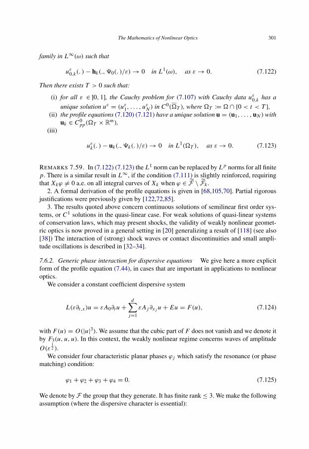
The Mathematics of Nonlinear Optics 301
family in L∞(ω) such that
uε0,k(. )− hk(., 90(. )/ε)→ 0 in L1(ω), as ε→ 0. (7.122)
Then there exists T > 0 such that:
(i) for all ε ∈ ]0, 1], the Cauchy problem for (7.107) with Cauchy data uε0,k has a
unique solution uε = (uε1, . . . , uεN ) in C0(�T ), where �T := � ∩ {0 < t < T },(ii) the profile equations (7.120) (7.121) have a unique solution u = (u1, . . . ,uN ) with
uk ∈ C0pp(�T × Rm),
(iii)
uεk(. )− uk(., 9k(. )/ε)→ 0 in L1(�T ), as ε→ 0. (7.123)
REMARKS 7.59. In (7.122) (7.123) the L1 norm can be replaced by L p norms for all finitep. There is a similar result in L∞, if the condition (7.111) is slightly reinforced, requiringthat Xkϕ 6= 0 a.e. on all integral curves of Xk when ϕ ∈ F \ Fk .
2. A formal derivation of the profile equations is given in [68,105,70]. Partial rigorousjustifications were previously given by [122,72,85].
3. The results quoted above concern continuous solutions of semilinear first order sys-tems, or C1 solutions in the quasi-linear case. For weak solutions of quasi-linear systemsof conservation laws, which may present shocks, the validity of weakly nonlinear geomet-ric optics is now proved in a general setting in [20] generalizing a result of [118] (see also[38]) The interaction of (strong) shock waves or contact discontinuities and small ampli-tude oscillations is described in [32–34].
7.6.2. Generic phase interaction for dispersive equations We give here a more explicitform of the profile equation (7.44), in cases that are important in applications to nonlinearoptics.
We consider a constant coefficient dispersive system
L(ε∂t,x )u = εA0∂t u +d∑
j=1
εA j∂x j u + Eu = F(u), (7.124)
with F(u) = O(|u|3). We assume that the cubic part of F does not vanish and we denote itby F3(u, u, u). In this context, the weakly nonlinear regime concerns waves of amplitude
O(ε12 ).
We consider four characteristic planar phases ϕ j which satisfy the resonance (or phasematching) condition:
ϕ1 + ϕ2 + ϕ3 + ϕ4 = 0. (7.125)
We denote by F the group that they generate. It has finite rank≤ 3. We make the followingassumption (where the dispersive character is essential):
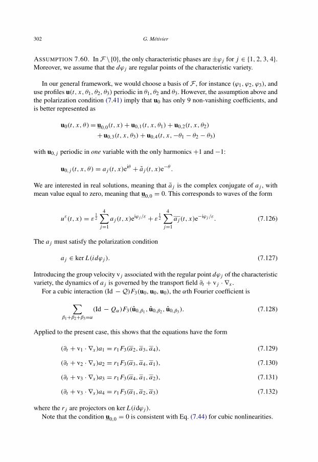
302 G. Metivier
ASSUMPTION 7.60. In F \{0}, the only characteristic phases are±ϕ j for j ∈ {1, 2, 3, 4}.Moreover, we assume that the dϕ j are regular points of the characteristic variety.
In our general framework, we would choose a basis of F , for instance (ϕ1, ϕ2, ϕ3), anduse profiles u(t, x, θ1, θ2, θ3) periodic in θ1, θ2 and θ3. However, the assumption above andthe polarization condition (7.41) imply that u0 has only 9 non-vanishing coefficients, andis better represented as
u0(t, x, θ)= u0,0(t, x)+ u0,1(t, x, θ1)+ u0,2(t, x, θ2)
+u0,3(t, x, θ3)+ u0,4(t, x,−θ1 − θ2 − θ3)
with u0, j periodic in one variable with the only harmonics +1 and −1:
u0, j (t, x, θ) = a j (t, x)eiθ+ a j (t, x)e−θ .
We are interested in real solutions, meaning that a j is the complex conjugate of a j , withmean value equal to zero, meaning that u0,0 = 0. This corresponds to waves of the form
uε(t, x) = ε12
4∑j=1
a j (t, x)eiϕ j /ε + ε12
4∑j=1
a j (t, x)e−iϕ j /ε. (7.126)
The a j must satisfy the polarization condition
a j ∈ ker L(idϕ j ). (7.127)
Introducing the group velocity v j associated with the regular point dϕ j of the characteristicvariety, the dynamics of a j is governed by the transport field ∂t + v j · ∇x .
For a cubic interaction (Id −Q)F3(u0,u0,u0), the αth Fourier coefficient is∑β1+β2+β3=α
(Id − Qα)F3(u0,β1 , u0,β2 , u0,β3). (7.128)
Applied to the present case, this shows that the equations have the form
(∂t + v1 · ∇x )a1 = r1 F3(a2, a3, a4), (7.129)
(∂t + v2 · ∇x )a2 = r1 F3(a3, a4, a1), (7.130)
(∂t + v3 · ∇x )a3 = r1 F3(a4, a1, a2), (7.131)
(∂t + v3 · ∇x )a4 = r1 F3(a1, a2, a3) (7.132)
where the r j are projectors on ker L(idϕ j ).Note that the condition u0,0 = 0 is consistent with Eq. (7.44) for cubic nonlinearities.

The Mathematics of Nonlinear Optics 303
This is the generic form of four wave interaction. There are analogues for three waveinteraction. These settings cover fundamental phenomena such as Raman scattering, Bril-louin scattering or Rayleigh scattering, see e.g. [6,10,107,109].
7.6.3. A model for Raman interaction We consider here a simplified model, based on aone dimensional version of the Maxwell–Bloch equation (see Section 2). The electric fieldE is assumed to have a constant direction, orthogonal to the direction of propagation. B isperpendicular both to E and the axis of propagation. The polarization P is parallel to E .This leads to the following set of equations∂t b + ∂x e = 0,
∂t e + ∂x b = −∂t tr(0ρ),iε∂tρ = [�, ρ] − e[0, ρ]
where e and b take their values in R and 0 is a Hermitian symmetric matrix, with entriesin C. In this case, note that tr(0[0, ρ]) = 0 and
ε∂t tr(0ρ) =1i
tr(0[�, ρ]).
A classical model to describe Raman scattering in one space dimension (see e.g. [10,107,109]) uses a three level model for the electrons, with � having three simple eigenvalues,ω1 < ω2 < ω3. Moreover, the states 1 and 2 have the same parity, while the state 3 hasthe opposite parity. This implies that the interaction coefficient γ1,2 vanishes. Finally, weassume that
� =
ω1 0 00 ω2 00 0 ω3
, 0 =
0 0 γ1,30 0 γ2,3γ3,1 γ3,2 0
.As noticed in Section 5.3.2, the scaling of the waves requires some care for Maxwell-
Bloch equations (see [73]). The density matrix ρ is assumed to be a perturbation of theground state
ρ =
1 0 00 0 00 0 0
.The scaling for amplitudes is
e = εe, b = εb,
ρ1,1 = 1+ ε2ρ1,1, ρ1,k = ερ1,k for k = 2, 3,
ρ j,k = ε2ρ j,k for 2 ≤ j, k ≤ 3.
(7.133)
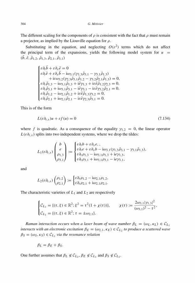
304 G. Metivier
The different scaling for the components of ρ is consistent with the fact that ρ must remaina projector, as implied by the Liouville equation for ρ.
Substituting in the equation, and neglecting O(ε2) terms which do not affectthe principal term of the expansions, yields the following model system for u =(b, e, ρ1,2, ρ1,3, ρ2,1, ρ3,1)
ε∂t b + ε∂x e = 0ε∂t e + ε∂x b − iω3,1(γ1,3ρ3,1 − γ3,1ρ1,3)
+ iεω3,2(γ2,3ρ3,1ρ1,2 − γ3,2ρ2,1ρ1,3) = 0,ε∂t ρ1,3 − iω3,1ρ1,3 + ieγ1,3 + iεeρ1,2γ2,3 = 0,ε∂t ρ3,1 + iω3,1ρ3,1 − ieγ3,1 − iεeγ3,2ρ2,1 = 0,ε∂t ρ1,2 − iω2,1ρ1,2 + iεeρ1,3γ3,2 = 0,ε∂t ρ2,1 + iω2,1ρ2,1 − iεeγ2,3ρ3,1 = 0.
This is of the form
L(ε∂t,x )u + ε f (u) = 0 (7.134)
where f is quadratic. As a consequence of the equality γ1,2 = 0, the linear operatorL(ε∂t,x ) splits into two independent systems, where we drop the tildes:
L1(ε∂t,x )
beρ1,3ρ3,1
:=ε∂t b + ε∂x e, ,ε∂t e + ε∂x b − iω3,1(γ1,3ρ3,1 − γ3,1ρ1,3),
ε∂tρ1,3 − iω3,1ρ1,3 + ieγ1,3,
ε∂tρ3,1 + iω3,1ρ3,1 − ieγ3,1,
and
L2(ε∂t,x )
(ρ1,2ρ2,1
):=
{ε∂tρ1,2 − iω2,1ρ1,2,
ε∂tρ2,1 + iω2,1ρ2,1.
The characteristic varieties of L1 and L2 are respectivelyCL1 = {(τ, ξ) ∈ R2; ξ2= τ 2(1+ χ(τ))}, χ(τ ) :=
2ω3,1|γ1,3|2
(ω3,1)2 − τ 2 ,
CL1 = {(τ, ξ) ∈ R2; τ = ±ω2,1}.
Raman interaction occurs when a laser beam of wave number βL = (ωL , κL) ∈ CL1
interacts with an electronic excitation βE = (ω2,1, κE ) ∈ CL2 to produce a scattered waveβS = (ωS, κS) ∈ CL1 via the resonance relation
βL = βE + βS .
One further assumes that βL 6∈ CL2 , βE 6∈ CL1 and βS 6∈ CL2 .

The Mathematics of Nonlinear Optics 305
We represent the oscillations, using the two independent phases
ϕL(t, x) = ωL t + κL x, ϕS(t, x) = ωS t + κS x .
The third phase ϕE is a linear combination of these two phases:
ϕE = ϕL − ϕS . (7.135)
Accordingly, we use profiles u depending on two fast variables θL and θS , so that
uε(t, x) ∼ u(t, y, ϕL/ε, ϕS/ε). (7.136)
Because f is quadratic, the conditions on (βL , βS, βE ) show that the profile equations havesolutions with spectra satisfying
spec(u) ⊂ {±(1, 0),±(0, 1),±(1,−1)}.
We now restrict our attention to these solutions. It is convenient to call u±L , u±S and u±E
the Fourier coefficients u±1,0, u0,±1 and u±1,∓1, respectively. Thus, for real solutions
uε(t, x)= uL(x)eiϕL (t,x)/ε + uS(x)eiϕS(t,x)/ε + uE (x)eiϕE (t,x)/ε
u−L(x)e−iϕL (t,x)/ε + u−S(x)e−iϕS(t,x)/ε + u−E (x)e−iϕE (t,x)/ε.
In addition, we use the notations bL , eL , ρ j,k,L for the components of uL etc.
LEMMA 7.61. The polarization conditions for the principal profile read
b±E = e±E = ρ1,3,±E = ρ3,1,±E = 0,
ρ1,2,±L = ρ1,2,±S = ρ2,1,±L = ρ2,1,±S = 0,
ρ1,2,−E = ρ2,1,E = 0,
(7.137)
and
bL = −1ωL
κLeL , ρ1,3,L =γ1,3
ω3,1 − ωLeL ,
ρ3,1,L =γ3,1
ω3,1 + ωLeL , (7.138)
with similar formula when L is replaced by −L and ±S. Furthermore, for real fields andHermitian density matrices, one has the relations
e−L = eL , e−S = eS, ρ2,1,−E = ρ1,2,E . (7.139)
Therefore, the profile equations for u0 involve only (eL , eS) and σE := ρ1,2,E :

306 G. Metivier
THEOREM 7.62. For real solutions, the evolution of the principal term is governed by thesystem (∂t + vL∂y)eL + ic1eSσE = 0,
(∂t + vS∂y)eS + ic2eSσE = 0,∂tσE + ic3eLeS = 0
(7.140)
where vL and vS are the group velocities associated with the frequencies βL and βS , re-spectively. The complete fields are recovered using the polarization conditions stated in thepreceding lemma.
This is the familiar form of the equations relative to three wave mixing. We refer, forexample, to [10,107] for an explicit calculation of the constants ck (see also [9]). The Ra-man instability (spontaneous or stimulated) is related to the amplification properties of thissystem.
7.6.4. Maximal dissipative equations For maximal dissipative systems, energy solutionsexist and are stable. In this context the weakly nonlinear approximations can be justifiedin the energy norm. The new point is that profiles need not be continuous, they belongto L p spaces, in which case the substitution θ = 9/ε has to be taken in the sense ofDefinition 7.11.
In R1+d , consider the Cauchy problem:
∂t u +d∑
j=1
A j∂ j u + f (u) = 0, u|t=0 = h. (7.141)
ASSUMPTION 7.63. The matrices A j are symmetric with constant coefficients and thedistinct eigenvalues λk(ξ) of A(ξ) =
∑ξ j A j have constant multiplicity for ξ 6= 0. We
denote by 5k the orthogonal spectral projector on ker A(ξ)− λk(ξ)Id .
ASSUMPTION 7.64 (Maximal monotonicity). f is a C1 function from CN to CN , withf (0) = 0 and there are p ∈ [1,+∞[ and constants 0 < c < C < +∞ such that for all(t, x) ∈ R1+d and all u and v in CN ,
| f (u)| ≤ C |u|p, |∂u,u f (u)| ≤ C |u|p−1,
Re (( f (u)− f (v)) · (u − v)) ≥ c|u − v|p+1.
Solutions of the Cauchy problem (7.141) are constructed in [121] (see also [99] or [61]):we consider smooth domains ω ⊂ Rd and � ⊂ [0 +∞[×Rdcontained in the domain ofdetermination of ω. The key ingredients are the energy estimates which follow from themonotonicity assumptions:
‖u(t)‖2L2 + c∫ t
0
∥∥u(t ′)∥∥p+1
L p+1 dt ′ ≤ ‖u(0)‖2L2 (7.142)

The Mathematics of Nonlinear Optics 307
and
‖u(t)− v(t)‖2L2 + c∫ t
0
∥∥u(t ′)− v(t ′)∥∥p+1
L p+1 dt ′ ≤ ‖u(0)− v(0)‖2L2 . (7.143)
PROPOSITION 7.65. For all h ∈ L2(ω), there is a unique solution of (7.141) u ∈C0L2
∩ L p+1(�).
We assume that the initial data have periodic oscillations
hε(x) ∼ h(x, ϕ0(x)/ε) (7.144)
with h(x, θ) periodic in θ ∈ T and ϕ0 ∈ C∞(ω) satisfying dϕ0(x) 6= 0 for all x ∈ ω. For1 ≤ k ≤ K , we denote by ϕk the solution of the eikonal equation
∂tϕk + λk(∂xϕk) = 0, ϕk |t=0 = ϕ0.
We assume that the space generated by the phases is weakly coherent and that no reso-nances occur:
ASSUMPTION 7.66. The ϕk are defined and smooth on� and dxϕk(x) 6= 0 at every point.Moreover,
For all α ∈ ZK , det L(dϕ(t, x)) 6= 0 a.e. on �, except when α belongs to one of thecoordinate axes.
Here L(∂t , ∂x ) = ∂t + A(∂x ). In this setting, the profiles are functions u(t, x, θ) whichare periodic in θ ∈ RK and periodic in θ . The projector P is
P∑
(uα(t, x)eiαθ ) =∑
Pα(uα(t, x)eiαθ )
and Pα is the orthogonal projector on ker L(α · 8). Introducing the averaging operator Ewith respect to all the variables θ , and Ek with respect to the all the variables except θk ,there holds
P u = Eu+K∑
k=1
5k(dϕk)Eku∗ (7.145)
with Eu = u0, the average of u, and u∗ = u− u0, its oscillation.The polarization conditions P u = u read
u(t, x, θ) = u(t, x)+K∑
k=1
u∗k(t, x, θk), u∗k = 5ku∗k (7.146)
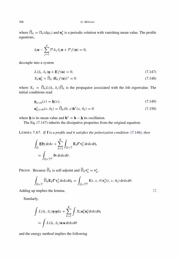
308 G. Metivier
where 5k = 5k(dϕk) and u∗k is a periodic solution with vanishing mean value. The profileequations,
∂t u−d∑
j=1
P A j∂ j u+ P f (u) = 0,
decouple into a system
L(∂t , ∂x )u+ E f (u) = 0, (7.147)
Xku∗k + 5k (Ek f (u))∗ = 0 (7.148)
where Xk = 5k L(∂t , ∂x )5k is the propagator associated with the kth eigenvalue. Theinitial conditions read
u|t=0(x) = h(x), (7.149)
u∗k |t=0(x, θk) = 5k(0, x)h∗(x, θk) = 0 (7.150)
where h is its mean value and h∗ = h− h its oscillation.The Eq. (7.147) inherits the dissipative properties from the original equation:
LEMMA 7.67. If f is a profile and v satisfies the polarization condition (7.146), then∫�
Efv dtdx +K∑
k=1
∫�×T
Ekf∗v∗k dtdxdθk
=
∫�×TK
fv dtdxdθ.
PROOF. Because 5k is self-adjoint and 5kv∗k = v∗k ,∫�×T
5kEkf∗v∗k dtdxdθk =
∫�×TK
f(t, x, θ)v∗k(t, x, θk) dtdxdθ.
Adding up implies the lemma. �
Similarly,
∫L(∂t , ∂x )u udx +
K∑k=1
∫Xku∗ku∗kdtdxdθk
=
∫L(∂t , ∂x )u u dtdxdθ
and the energy method implies the following

The Mathematics of Nonlinear Optics 309
PROPOSITION 7.68. For all h ∈ L2(ω×T), there is a unique u ∈ C0L2∩ L p+1(�×TK )
of the form (7.146), and satisfying the profile equations (7.147) (7.148), with initial data(7.149) (7.150).
Knowing u, one can construct
vε(t, x) ∼ u(t, x,8(t, x)/ε), (7.151)
not performing directly the substitution θ = 8/ε in u(t, x, θ), since this function is notnecessarily continuous in θ , but in the sense of Definition 7.11: the family (vε) is F oscil-lating with profile u, where F is the group generated by the ϕk . The asymptotic in (7.151)is taken in L p+1(�) and in C0L2(�).
A key observation is that since u solves the profile equation, one can select vε satisfyingapproximately the original equation (in the spirit of Section 7.3.6):
PROPOSITION 7.69. There is a bounded family vε in C0L2(�)∩ L p+1(�), F oscillatingwith profile u and such that∥∥L(∂t , ∂x )v
ε+ f (vε)
∥∥L1+1/p(�)
→ 0, as ε→ 0.
Using the monotonicity of the equation, one can compare vε with the exact solution uε
given by Proposition 7.65:
∥∥uε(t)− vε(t)∥∥2
L2 + c∫ t
0
∥∥uε(t ′)− vε(t ′)∥∥p+1
L p+1 dt ′
≤∥∥uε(0)− vε(0)
∥∥2L2 + c
∫ t
0
∥∥Lvε + (vε)(t ′)∥∥1+1/p
L1+1/p dt ′.
This implies the following result.
THEOREM 7.70. Suppose that h ∈ L2(ω) and that the family hε satisfies (7.144) in L2.Let u denote the solution of the profile equation and (uε) the family of solutions of (7.141)with initial data (hε). Then uε satisfies (7.151) in L p+1(�) ∩ C0L2(�).
This method, inspired from [48], is extended in [79,80] to analyze oscillations in thepresence of caustics and in [21] to study oscillations near a diffractive boundary point. Forthe nonlinear problem, no L∞ description is known near caustics or diffractive boundarypoints. The method sketched above applies to energy solutions but provides only asymp-totics in L p spaces with p <∞.
References
[1] G. Alı, J.K. Hunter, Large amplitude gravitational waves, J. Math. Phys. 40 (1999) 3035–3052.[2] D. Alterman, J. Rauch, Nonlinear geometric optics for short pulses, J. Differential Equations 178 (2002)
437–465.

310 G. Metivier
[3] D. Alterman, J. Rauch, Diffractive nonlinear geometric optics for short pulses, SIAM J. Math. Anal. 34(2003) 147–1502.
[4] M. Artola, A.J. Majda, Nonlinear development of instabilities in supersonic vortex sheets I. The basickink mode, Physica D 28 (1987) 253–281.
[5] W. Blaschke, G. Bol, Geometrie der Gewebe, New York, Springer-Verlag, 1938.[6] N. Bloembergen, Nonlinear Optics, W.A. Benjamin Inc., New York, 1965.[7] J. Bona, T. Colin, D. Lannes, Long wave approximations for water waves, in: Mathematical and Numerical
Aspects of Wave Propagation, WAVES 2003, Springer, Berlin, 2003, pp. 489–494.[8] M. Born, E. Wolf, Principles of Optics, Pergamon Press, 1959.[9] T. Boucheres, T. Colin, B. Nkonga, B. Texier, A. Bourgeade, Study of a mathematical model for stimulated
Raman scattering, Math. Models Methods Appl. Sci. 14 (2004) 217–252.[10] R. Boyd, Nonlinear Optics, Academic Press, 1992.[11] G. Browning, H.-O. Kreiss, Problems with different time scales for non-linear partial differential
equations, SIAM J. Appl. Math. 42 (1982) 704–718.[12] R. Carles, Comportements precises pres d’une caustique en optique geometrique non lineaire, Comm.
Partial Differential Equations 23 (1998) 1929–1967.[13] R. Carles, Geometric optics with caustic crossing for some nonlinear Schrodinger equations, Indiana
Univ. Math. J. 49 (2000) 475–551.[14] R. Carles, Focusing on a line for nonlinear Schrodinger equations in R2, Asymptot. Anal. 24 (2000)
255–276.[15] R. Carles, Semi-classical Analysis for Nonlinear Schrodinger Equations, World Scientific Publishing Co.
Pte. Ltd., Hackensack, NJ, 2008.[16] R. Carles, D. Lannes, Focusing of a pulse with arbitrary phase shift for a nonlinear wave equation, Bull.
Soc. Math. France 131 (2003) 289–306.[17] R. Carles, J. Rauch, Focusing of spherical nonlinear pulses in R1+3, Proc. Amer. Math. Soc. 130 (2002)
791–804.[18] R. Carles, J. Rauch, Focusing of spherical nonlinear pulses in R1/3 II. Nonlinear caustic, Rev. Mat.
Iberoamericana 20 (2004) 815–864.[19] R. Carles, J. Rauch, Focusing of spherical nonlinear pulses in R1+3. III. Sub and supercritical cases,
Tohoku Math. J. 56 (2004) 393–410.[20] C. Cheverry, Justification de l’optique geometrique non lineaire pour un systıme de lois de conservation,
Duke Math. J. 87 (1997) 213–263.[21] C. Cheverry, Propagation d’oscillations pres d’un point diffractif , J. Maths. Pures et Appl. 75 (1996)
419–467.[22] C. Cheverry, Cascade of phases in turbulent flows, Bull. Soc. Math. France 134 (1) (2006) 33–82.[23] C. Cheverry, O. Gues, G. Metivier, Oscillations fortes sur un chamlineairement degenere, Ann. Sc. Ecol.
Norm. Sup. 36 (2003) 691–745.[24] C. Cheverry, O. Gues, G. Metivier, Large amplitude high frequency waves for quasilinear hyperbolic
equations, Adv. Differential Equations 9 (2004) 829–890.[25] J. Chikhi, Sur la reflexion des oscillations pour un systeme a deux vitesses, C. R. Acad. Sci. Paris Ser. I
Math. 313 (1991) 675–678.[26] Y. Choquet-Bruhat, Construction de solutions radiatives approchees des equations d’Einsein, Comm.
Math. Phys. 12 (1969) 16–35.[27] Y. Choquet-Bruhat, A. Greco, High frequency asymptotic solutions of Y.M. and associated fields, J. Math.
Phys 24 (1983) 337–379.[28] T. Colin, Rigorous derivation of the nonlinear Schrodinger equation and Davey–Stewartson systems from
quadratic hyperbolic systems, Asymptot. Anal. 31 (2002) 69–91.[29] M. Colin, T. Colin, On a quasilinear Zakharov System describing laser-plasma interactions, Differential
Integral Equations 17 (2004) 297–330.[30] T. Colin, D. Lannes, Long-wave short-wave resonance for nonlinear geometric optics, Duke Math. J. 107
(2) (2001) 351–419.[31] T. Colin, D. Lannes, Justification of and longwave correction to Davey–Stewartson systems from quadratic
hyperbolic systems, Discrete Contin. Dyn. Syst. 11 (2004) 83–100.[32] A. Corli, Weakly non-linear geometric optics for hyperbolic systems of conservation laws with shock
waves, Asymptot. Anal. 10 (1995) 117–172.[33] A. Corli, Asymptotic analysis of contact discontinuities, Ann. Mat. Pura Appl. 173 (1997) 163–202.

The Mathematics of Nonlinear Optics 311
[34] A. Corli, O. Gues, Stratified solutions for systems of conservation laws, Trans. Amer. Math. Soc. 353 (6)(2001) 2459–2486.
[35] R. Courant, K.O. Friedrichs, Supersonic Flow and Shock Waves, Wiley-Interscience, New York, 1948.[36] R. Courant, D. Hilbert, Methods of Mathematical Physics, John Wiley & Sons, New York, 1962.[37] J.-L. Delcroix, A. Bers, Physique des plasmas 1, 2, Inter Editions-Editions du CNRS, 1994 .[38] R.J. DiPerna, A.J. Majda, The validity of nonlinear geometric optics for weak solutions of conservation
laws, Comm. Math. Phys. 98 (1985) 313–347.[39] P. Donnat, Quelques contributions mathematiques en optique non lineaire, These, Ecole Polytechnique,
1994 .[40] P. Donnat, J.-L. Joly, G. Metivier, J. Rauch, Diffractive nonlinear optics, Seminaire E.D.P., Ecole
Polytechnique 1995–96.[41] P. Donnat, J. Rauch, Dispersive nonlinear geometric optics, J. Math. Phys. 38 (1997) 1484–1523.[42] P. Donnat, J. Rauch, Global solvability of the Maxwell Bloch equations from nonlinear optics, Arch.
Rational Mech. Anal 136 (3) (1996) 291–303.[43] J.J. Duistermaat, Oscillatory integrals, Lagrangian immersions and unfolding of singularities, Comm.
Pure Appl. Math. 27 (1974) 207–281.[44] E. Dumas, Periodic multiphase nonlinear diffactive optics with curved phases, Indiana Univ. Math. J. 52
(2003) 769–810.[45] E. Dumas, Nonlinear diffactive optics with curved phases: Beam dispersion and transition between light
and shadow, Asymptot. Anal. 38 (204) 47–91 .[46] E. Dumas, Global existence for Maxwell–Bloch systems, J. Differential Equations 219 (2005) 484–509.[47] W.E. Propagation of oscillations in the solutions of 1 − D compressible fluid equations, Comm. Partial
Differential Equations 17 (3–4) (1992) 347–370.[48] L.C. Evans, Weak Convergence Methods for Non Linear Partial Differential Equations, AMS, Providence,
RI, 1990.[49] R.P. Feynmann, Lectures on Physics, vols. I and II, Addison-Wesley, 1963, and 1964.[50] K.O. Friedrichs, Symmetric hyperbolic linear differential equations, Comm. Pure Appl. Math. 7 (1954)
345–392.[51] K.O. Friedrichs, Symmetric positive linear differential equations, Comm. Pure Appl. Math. 11 (1958)
333–418.[52] K.O. Friedrichs, Nonlinear hyperbolic differential equations for functions of two independent variables,
Amer. J. Math. 70 (1948) 555–589.[53] K.O. Friedrichs, P.D. Lax, Systems of conservation laws with a convex extension, Proc. Nat. Acad. Sc.
USA 68 (1971) 1686–1688.[54] S. Friedlander, W. Strauss, M. Vishik, Nonlinear instability in an ideal fluid, Ann. Inst. Henri Poincare 14
(2) (1997) 187–209.[55] L. Garding, Problemes de Cauchy pour des systemes quasi-lineaires d’ordre un, strictement hyperboliques,
dans Les EDP, Colloques Internationaux du CNRS, 117, 1963, pp. 33–40.[56] P. Godin, Global oscillatory waves for second order quasilinear wave equations, Trans. Amer. Math. Soc.
346 (2) (1994) 523–547.[57] E. Grenier, On the nonlinear instability of Euler and Prandtl equations, Comm. Pure Appl. Math. 53 (9)
(2000) 1067–1091.[58] O. Gues, Probleme mixte hyperbolique quasilineaire caracteristique, Comm. Partial Differential
Equations 15 (1990) 595–645.[59] O. Gues, Ondes multidimensionnelles ε- stratifiees et oscillations, Duke Math. J. 68 (3) (1992) 401–446.[60] O. Gues, Developpement asymptotique de solutions exactes de systemes hyperboliques quasilineaires,
Asymptot. Anal. 6 (3) (1993) 241–269.[61] A. Haraux, Semilinear Hyperbolic Problems in Bounded Domains, in: Mathematical Reports, vol. 3, Part
1, Harwood Academic Publishers, 1987.[62] A. Heibig, Error estimates for oscillatory solutions to hyperbolic systems of conservation laws, Comm.
Partial Differential Equations 18 (1993) 281–304.[63] E. Hewitt, K.A. Ross, Abstract Harmonic Analysis, vol. 1, Springer-Verlag, Berlin, 1963.[64] L. Hormander, Fourier Integral Operators I, Acta. Math. 127 (1971) 79–183.[65] L. Hormander, The Analysis of Linear Partial Differential Operators, Springer, 1990.[66] L. Hormander, Lectures on Nonlinear Hyperbolic Differential Equations, in: Mathematiques et Applica-
tions, vol. 26, Sringer Verlag, 1997.

312 G. Metivier
[67] J.K. Hunter, Transverse diffraction of nonlinear waves and singular rays, SIAM J. Appl. Math. 48 (1988)1–37.
[68] J.K. Hunter, J.B. Keller, Weakly nonlinear high frequency waves, Comm. Pure Appl. Math. 36 (1983)547–569.
[69] J.K. Hunter, J.B. Keller, Caustics of nonlinear waves, Wave Motion 9 (1987) 429–443.[70] J.K. Hunter, A.J. Majda, R. Rosales, Resonantly interacting weakly nonlinear hyperbolic waves II:
Several space variables, Stud. Appl. Math. 75 (1986) 187–226.[71] P.-Y. Jeanne, Optique geometrique pour des systemes semi-lineaires avec invariance de jauge, Mem. Soc.
Math. France (2002) 9–160.[72] J.-L. Joly, Sur la propagations des oscillations semi-lineares en dimension 1 d’espace, C. R. Acad. Sc.
Paris t. 296 (1983).[73] J.-L. Joly, G. Metivier, J. Rauch, Transparent nonlinear geometric optics and Maxwell–Bloch equations,
J. Differential Equations 166 (2000) 175–250.[74] J.-L. Joly, G. Metivier, J. Rauch, Generic rigorous asymptotic expansions for weakly nonlinear geometric
optics, Duke. Math. J. 70 (1993) 373–404.[75] J.-L. Joly, G. Metivier, J. Rauch, Coherent nonlinear waves and the Wiener algebra, Ann. Inst. Fourier
44 (1994) 167–196.[76] J.-L. Joly, G. Metivier, J. Rauch, Coherent and focusing multidimensional nonlinear geometric optics,
Ann. Sci. Ecole Norm. Sup. (4) 28 (1) (1995) 51–113.[77] J.-L. Joly, G. Metivier, J. Rauch, Global existence for anharmonic nonlinear Maxwell equations, SIAM
J. Math. Anal. 27 (1996) 905–913.[78] J.-L. Joly, G. Metivier, J. Rauch, Focusing at a point and absorption of nonlinear oscillations, Trans.
Amer. Math. Soc. 347 (1995) 3921–3971.[79] J.-L. Joly, G. Metivier, J. Rauch, Nonlinear oscillations beyond caustics, Comm. Pure Appl. Math. 48
(1996) 443–529.[80] J.-L. Joly, G. Metivier, J. Rauch, Caustics for dissipative semilinear oscillations, Mem. Amer. Math. Soc.
(685) (2000).[81] J.-L. Joly, G. Metivier, J. Rauch, Diffractive geometric optics with rectification, Indiana Math. J. 47
(1998) 1167–1241.[82] J.-L. Joly, G. Metivier, J. Rauch, Resonant one dimensional nonlinear geometric optics, J. Funct. Anal.
114 (1993) 106–231.[83] J.-L. Joly, G. Metivier, J. Rauch, Global solutions to Maxwell equations in a ferromagnetic medium, Ann.
Henri Poincare 1 (2000) 307–340.[84] J.-L. Joly, G. Metivier, J. Rauch, Hyperbolic domains of determinacy and Hamilton–Jacobi equations, J.
Hyperbolic 1 Differential Equations 2 (2005) 1–32.[85] L.A. Kalyakin, Long wave asymptotics integrable equations as asymptotic limit of nonlinear systems,
Russian Math. Surveys 44 (1) (1989) 3–42.[86] S. Klainerman, A.J. Majda, Singular perturbations of quasilinear hyperbolic systems with large param-
eters and the incompressible limit of compressible fluids, Comm. Pure Appl. Math. 34 (1981) 481–524.[87] S. Klainerman, A.J. Majda, Compressible and incompressible fluids, Comm. Pure Appl. Math. 35 (1982)
629–653.[88] H.-O. Kreiss, J. Lorenz, M.J. Naughton, Convergence of the solutions of the compressible to the solutions
of the incompressible Navier–Stokes equations, Adv. in Appl. Math. 12 (1991) 187–214.[89] L.D. Landau, E.M. Lifshitz, Electrodynamique des milieux continus Physique theorique (008), Mir, New
York, 1969.[90] D. Lannes, Dispersive effects for nonlinear geometrical optics with rectification, Asympt. Anal. 18 (1998)
111–116.[91] D. Lannes, Consistency of the KP approximation, Discrete Contin. Dyn. Syst. (2003) 517–525.[92] P.D. Lax, Asymptotic solutions of oscillatory initial value problems, Duke Math. J. 24 (1957) 627–645.[93] P.D. Lax, Lectures on Hyperbolic Partial Differential Equations, Stanford, 1963.[94] P.D. Lax, R. Phillips, Local boundary conditions for dissipative symmetric linear differential operators,
Comm. Pure and Appl. Math. 13 (1960) 427–455.[95] G. Lebeau, Nonlinear optic and supercritical wave equation, Bull. Soc. Math. Liege 70 (2001) 267–306.[96] J. Leray, Hyperbolic Differential Equations, Institute for Advanced Study, 1953.[97] V. Lescaret, Wave transmission in dispersive media, Math. Models Methods Appl. Sci. 17 (2007) 485–535.

The Mathematics of Nonlinear Optics 313
[98] V. Lescaret, Diffractive wave transmission in dispersive media, J. Differential Equations 244 (2008)972–1010.
[99] J.-L. Lions, W. Strauss, Some nonlinear evolution equations, Bull. Soc. Math. France 93 (1965) 43–96.[100] H.A. Lorentz, The Theory of Electrons, 2nd edition, Teubner, 1908, Reprinted by Dover, 1952.[101] D. Ludwig, Uniform asymptotic expansions at a caustic, Comm. Pure Appl. Math 19 (1966) 215–250.[102] D. Ludwig, Conical refraction in crystal optics and hydromagnetics, Comm. Pure Appl. Math 14 (1961)
113–124.[103] A.J. Majda, Compressible Fluid Flow and Systems of Conservation Laws in Several Space Variables,
Springer-Verlag, New York, 1984.[104] A.J. Majda, M. Artola, Nonlinear geometric optics for hyperbolic mixed problems, in: Analyse
Mathematique et Applications, Gauthuier-Villars, Paris, 1988, pp. 319–356.[105] A.J. Majda, R. Rosales, Resonantly interacting weakly nonlinear hyperbolic waves I: A single space
variable, Stud. Appl. Math. 71 (1984) 149–179.[106] S. Mizohata, On the Cauchy Problem, in: Notes and Reports in Mathematics in Science an Engineering,
vol. 3, Academic Press, 1985.[107] A. Newell, J. Moloney, Nonlinear Optics, Addison-Wesley, Reading Mass, 1992.[108] A. Owyoung, The Origin of the nonlinear refractive indices of liquids and glasses, Ph.D Dissertation
Caltech, 1971 .[109] R. Pantell, H. Puthoff, Fundamentals of Quantum Electronics, J. Wiley & Sons Inc., New York, 1973;
Electronique quantitique en vue des applications, Dunod.[110] Y.-J. Peng, Solutions faibles globales pour l’equation d’Euler d’un fluide compressible avec de grandes
donnees initiales, Comm. Partial Differential Equations 17 (1992) 161–187.[111] Sur les surfaces de translation et les fonctions Abeliennes, Bull. Soc. Math. France 29 (1901) 61–86.[112] J. Rauch, BV estimates fail for most quasilinear hyperbolic systems in dimensions greater than one,
Comm. Math. Phys. 106 (1986) 481–484.[113] J. Rauch, Symmetric positive systems with boundary characteristic of constant multiplicity, Trans. Amer.
Math. Soc. 291 (1985) 167–187.[114] J. Rauch, Lectures on geometric optics, IAS-Park City Summer School on Nonlinear Waves, July, 1995 .[115] S. Schochet, The compressible Euler equations in a bounded domain: existence of solutions and the
incompressible limit, Commun. Math. Phys 104 (1986) 49–75.[116] S. Schochet, Asymptotics for symmetric hyperbolic systems with a large parameter, J. Differential
Equations 75 (1988) 1–27.[117] S. Schochet, Fast singular limits of hyperbolic PDEs, J. Differential Equations 114 (1994) 476–512.[118] S. Schochet, Resonant nonlinear geometric optics for weak solutions of conservation laws, J. Differential
Equations 113 (1994) 473–504.[119] D. Serre, Oscillations nonlineaires de haute frequence. Dim ≥ 2, in: A. Marino, M.K.V. Murthy (Eds.),
Nonlinear Variational Problems and Partial Differential Equations, in: Pitman Res. Notes in Math., vol.320, Longman, London, 1995, pp. 245–294, Springer-Verlag, New-York, 1983.
[120] B. Sevennec, Geometrie des systemes hyperboliques de lois de conservation, Societe mathematique deFrance, Memoire 56, Suppl. Bull. Soc. Math. France 122 (1) (1994).
[121] W. Strauss, The energy method in nonlinear partial differential equations, Notas de matematica 47,Instituto de Matematica Pura e Applicata, Rio de Janeiro 1969 .
[122] L. Tartar, Solutions oscillantes des equations de Carleman, Seminaire Goulaouic–Schwartz, EcolePolytechnique, Paris, annee 1980-0981 .
[123] M. Taylor, Partial Differential Equations III, in: Applied Mathematical Sciences, vol. 117, Springer, 1996.[124] B. Texier, The short-wave limit for nonlinear symmetric hyperbolic systems, Adv. Differential Equations
9 (2004) 1–52.[125] B. Texier, WKB asymptotics for the Euler–Maxwell equations, Asymptot. Anal. 42 (2005) 211–250.[126] A. Weil, L’integration dans les groupes topologiques et ses applications, Hermann, Paris, 1940.[127] G.B. Witham, Nonlinear Waves, in: Wiley-Intersciences Series of Texts, John Wiley and Sons, 1993.[128] M. Williams, Resonant reflection of multidimensional semilinear oscillations, Comm. in Partial Diff. Equ.
18 (1993) 1901–1959.[129] M. Williams, Boundary layers and glancing blow-up in nonlinear geometric optics, Ann. Sci. Ecole
Norm. Sup. 33 (2000) 383–432.