The mass balance and equilibrium line altitude trends...

Student thesis series INES nr 418

Caroline Hall

2017

Department of

Physical Geography and Ecosystem Science

Lund University

Sölvegatan 12

S-223 62 Lund

Sweden

The mass balance and equilibrium line altitude trends of glaciers in northern Sweden

Caroline Hall (2017)


Bachelor degree thesis, 30 credits in Physical Geography and Ecosystem Science

Department of Physical Geography and Ecosystem Science, Lund University

Level: Bachelor of Science (BSc)

Course duration: March 2017 until June 2017

Disclaimer

This document describes work undertaken as part of a program of study at the University of Lund. All views and opinions expressed herein remain the sole responsibility of the author, and do not necessarily represent those of the institute.

Photograph: The Tarfala study area in August 2016. Taken by Hanna Ribjer.


Caroline Hall

Bachelor thesis, 30 credits, in Physical geography and ecosystem science

Supervisor:

Margareta Johansson, Lund University

Exam committee:

Andrew McRobert, Lund University

Vaughan Phillips, Lund University

Abstract Glaciers are of extreme importance since they hold climatic data going back 2,000 years. Glaciers can provide important services such as ecosystem services, habitats, water runoff, and hydro-energy. They also affect the Earth’s processes and many feedback mechanisms. Glaciers all over the world are under the threat of climate change which may eventually lead to the disappearance of many of these important glaciers. That is why it is important to understand glaciological processes and to understand how individual glaciers are affected by climatic changes.

This study focuses on the glaciers in northern Sweden and their response to climatic changes over a 15 year period (1986-2011). Data from the Tarfala research station, in northern Sweden is used to find trends in winter and summer mass balance, net mass balance and equilibrium line altitude. The reasons for similarities and differences in the trends are discussed and the glacial parameters are compared with parameters such as elevation, location, and aspect.

Overall it was found that the winter balances were decreasing, the summer balances were increasing and the net mass balances were decreasing which results in a loss of mass on all glaciers. The differences amongst the glaciers were attributed to differences in altitude, location and climate. Also, R2 values and p-values showed that a significant relationship exists between the net mass balance and the summer temperature proving that the summer temperature is the main factor affecting mass loss or gain on glaciers in northern Sweden.

Although the aim of the study was achieved, there were some limitations to it such as lack of or incomplete data, missing parameters and limited factors considered and compared. Future studies should include wind speeds and direction, solar radiation and humidity to name a few. Also, not only should the net mass balance and equilibrium line altitudes be analysed, but thickness, volume and frontal positions should be considered.

Key words Glaciers, Sweden, accumulation, ablation, net mass balance, equilibrium line altitude (ELA), climate, precipitation, temperature.

Contents Abstract ............................................................................................................................................... 4 Key words ........................................................................................................................................... 4 1. Introduction ................................................................................................................................ 1

1.2 Aim ........................................................................................................................................... 1 2. Background ................................................................................................................................ 2

2.1 Accumulation, ablation and net mass balance .......................................................................... 2 2.2 Equilibrium line altitude ........................................................................................................... 2 2.3 The importance of glaciers and glacial parameters ................................................................... 2 2.4 Climatic history ......................................................................................................................... 3

3. Study area .................................................................................................................................. 3 3.1 General description ................................................................................................................... 3 3.2 Geology and bedrock ................................................................................................................ 5 3.3 Soil and vegetation .................................................................................................................... 6 3.4 Climate ...................................................................................................................................... 6 3.5 The glaciers ............................................................................................................................... 9

4. Methodology ............................................................................................................................ 13 4.1 Data ......................................................................................................................................... 13 4.2 Data preparation ...................................................................................................................... 14 4.3 Statistical analyses .................................................................................................................. 15

5. Results ...................................................................................................................................... 15 5.1 Winter mass balance ............................................................................................................... 15 5.2 Summer mass balance ............................................................................................................. 16 5.3 Net mass balance ..................................................................................................................... 18 5.4 Equilibrium line altitude ......................................................................................................... 19 5.5 Parameters affecting mass balance ......................................................................................... 21

6. Discussion ............................................................................................................................... 22 6.1 Summer and winter mass balances ......................................................................................... 22 6.2 Net mass balance ..................................................................................................................... 24 6.3 Equilibrium line altitude ......................................................................................................... 25 6.4 Parameters affecting mass balance. ........................................................................................ 26 6.5 Limitations .............................................................................................................................. 27 6.6 Further studies ......................................................................................................................... 28

7. Conclusion ............................................................................................................................... 28 8. Acknowledgements .................................................................................................................. 29 9. References ................................................................................................................................ 30 10. Appendix ............................................................................................................................. 33

1

1. Introduction The glaciers of northern Sweden provide great knowledge about past and present climate. Not only do they represent the climatic changes of today but they also reflect the climatic changes which occurred hundreds of years ago. In the ice caps of Antarctica and Greenland, ice cores have revealed some information about global climate going back 800,000 years (Lüthi et al. 2008; Parrenin et al. 2007). However, in northern Sweden, the ice cores retrieved so far have been much smaller and therefore can only reveal data dating back 2,000 years (Auger and Grigholm 2017). With the changing climate and increasing carbon dioxide concentrations, glaciers all over the world are likely to retreat at a fast rate and may eventually disappear. Climate scenarios have implied that climate change will affect polar regions such as the Arctic much more than other regions (Holland and Bitz 2003). This is why glaciers could be used as markers for the severity of the change. Whilst many studies support this theory (Arendt et al. 2002; Oerlemans 2005), others are more sceptical since they believe that there is not enough understanding of how glaciers respond to climate change (Dowdeswell et al. 1997; Dyurgeroc and Meier 2000; Abdalati 2004). The glaciers in northern Sweden, along with the glaciers in Norway, Russia, Alaska, Canada, and Finland can provide an overview of the trends in glacial changes in the Arctic and can therefore be used to model future changes (Olsen et al. 2011). Studying the glaciers of the Arctic is of extreme importance since they affect so many of the Earth’s processes: air and ocean circulation, regulation of freshwater, storage and release of greenhouse gases, sea level changes, and therefore the shape and extent of the Earth’s land masses (Olsen et al. 2011). The glaciers in the Arctic and in northern Sweden have previously been studied. In Sweden, most of the studies date from the 1940s-1990s. It has been found that the climate in the area has changed over the past 100 years. Also, the mass balance, summer and winter mass balances and equilibrium line altitude have also been studied. Overall, the glaciers have been retreating although some reached a steady state in the 1970s and 1990s (Holmlund and Jansson 1999).

The current study of glaciers is relevant since glaciers today are still adjusting to climatic changes from the beginning of the 20th century (Holmlund et al. 1996). This means that glaciers will still be adjusting to the recent climate changes hundreds of years from now. The consequences of this could be huge and it is therefore important to understand glacial processes (particularly thermic and dynamic) and how glaciers change with a changing climate and how these will come to affect the shape and size of glaciers in the future (Cuffey and Paterson 2010).

1.2 Aim The aim of this study is to evaluate the evolution of glaciers in northern Sweden in terms of their mass balance. This study will focus on five glaciers: Tarfalaglaciären, Storglaciären, Riukojietna, Rabots glaciär, and Mårmaglaciären. Trends in winter mass balance, summer mass balance, net mass balance, and the elevation line altitude (ELA) will be examined and will be compared with parameters such as elevation and aspect to find the reasons for the differences in trends amongst the glaciers.

It is expected that in this area, the winter mass balance has decreased, the summer mass balance has increased and the net mass balance has decreased over the entire period

2

(Holmlund et al. 1996). It is also expected that the ELA has become higher in elevation (Cuffey and Paterson 2010).

2. Background 2.1 Accumulation, ablation and net mass balance Glaciers lose and gain mass throughout the year and the amount that they gain or lose determines whether they shrink or grow. Although every glacier is different and complex, it is possible to divide the glacier into two main zones: the accumulation zone and the ablation zone. The accumulation zone represents the winter mass balance and is mostly situated at the top area of the glacier where all processes by which snow and ice are added to the glacier occur. This is where the glacier grows and thickens. Accumulation occurs through deposition of snow and rain, wind deposition, refreezing of water and avalanche deposition (Cuffey and Paterson 2010). Accumulation can also occur in the lower part of the glacier (the ablation zone) through avalanching and precipitation. The ablation zone on the other hand represents the summer mass balance and is the lower area of the glacier where the processes of loss occur and therefore where the glacier shrinks and thins. Ablation occurs through sublimation, melt, and calving (Cuffey and Paterson 2010). The net mass balance of a glacier generally refers to the net difference between accumulation and ablation which means that it is possible to know whether a glacier is losing or gaining mass. If the accumulation is bigger than the ablation, the glacier is gaining mass. If the opposite is true, the glacier is losing mass (Cuffey and Paterson 2010). A steady state is reached when the net mass balance of a glacier stays at zero for many years. This means that the shape and area of the glacier does not change and the glacier is in perfect equilibrium with the past and present climate. Generally, the bigger the glacier is, the longer it must have a zero net mass balance to be in a steady state (Cuffey and Paterson 2010). This theoretical idea never happens in reality which is why glaciers can never be in a “steady-state” but can be in a “near steady-state”.

2.2 Equilibrium line altitude The boundary between the accumulation and ablation zones is called the equilibrium line and when the altitude of the line is considered it is called the equilibrium line altitude (ELA). As a glacier shrinks, the ELA will move further up in altitude. The ELA is a suitable but imprecise way to assess the changes of glaciers (Kuhn et al. 1999). This is because it helps to determine whether the accumulation and ablation zones are approximately getting bigger or smaller, but it does not take areal or frontal changes into account. Also, the ELA is not a physical line, it is more of a general area or boundary where changes can be seen. Also, this boundary does not run at the same altitude throughout the glacier so an average for the entire glacier (Singh et al. 2011). 2.3 The importance of glaciers and glacial parameters The study of accumulation, ablation and net mass balance is extremely important, not just because it helps to identify trends of mass loss or gain, but also because when looked at in terms of water equivalent, the mass balance can reflect trends in sea level changes (Cuffey and Paterson 2010). The glaciers of northern Sweden on their own cannot reflect such patterns, but when taken into account with Norwegian, Russian, Canadian, and Alaskan glaciers it is possible to find trends for the Arctic glaciers. Olsen et al. (2011) found that the mountain glaciers in the Arctic had lost over 150 Gt of mass per year for the years 2000-2011, which made them a significant contributor to the global sea level changes.

3

Moreover, glacial retreat and advance lead to changes in runoff. As a glacier retreats, it first increases the amount of runoff water but as soon as the glacier disappears, the runoff stops (Jansson et al. 2003). This will have effects on the vegetation of the area and alter the ecosystems and impact species habitats (Olsen et al. 2011). The disappearance of glaciers could significantly affect the ecosystem of the region and change its landscape (Hood and Berner 2009). The melting of glaciers and sea ice may have positive impacts. For example, it may lead to more water becoming available and producing more hydro-energy or it could lead to better access to the Arctic leading to increased tourism and shipping. It could negatively affect the population living in these areas whom rely on the services provided by the glaciers and their associated runoff. Changes to the Arctic cryosphere could impact the culture, identity, livelihood, economies, and health of the populations and areas close to glaciers (Olsen et al. 2011).

2.4 Climatic history To understand the changes in glacial retreat and advance, it is important to look back at the climate. Although climatic fluctuations have happened for thousands and millions of years, the past 200 years are the most important here (Holmlund and Jansson 1999). Going back to the 19th century, the climate in northern Sweden was overall drier and colder than today. At the end of the century and the beginning of the 20th century, the climate became more maritime (more precipitation and humidity) and therefore glaciers began to expand. Most glaciers reached their Holocene maximum at this point. However, between 1910 and 1920, the summer temperatures increased by almost 1 ͦ C which led to glaciers retreating at a quick pace. Low ablation rates at the time means that many glaciers are still adjusting to this drastic temperature change. The climate between the 1920s and 1980s remained relatively stable although the temperature maximum was reached at the end of the 1930s. This allowed for some glaciers such as Storglaciären to reach a near steady-state in the 1970s. In the mid-1980s, a slight cooling meant that the accumulation rates increased (just like a hundred years before). This led to some smaller glaciers thickening (Holmlund and Jansson 1999). Also, due to increased precipitation in the late 1980s and early 1990s, the frontal retreat which had been occurring on glaciers started to slow down or even stop altogether leading to some glaciers reaching a near steady-state once again in the 1990s (Holmlund et al. 1996).

Since the 1990s however, the climate has seen an increase in temperature (see figure 5 in section 3.4) which has led to a thinning trend (in summer months particularly). The changes seen at end of the 20th century have not been reflected in the glacial front positions. However, since they are still reacting to the warming of the 1910s this is likely to occur at a later stage (Holmlund and Jansson 1999).

3. Study area 3.1 General description The study area is located in northern Sweden in Kiruna municipality, in the Norrbotten County. Kiruna municipality is the northernmost county in Sweden which means that it lies above the Arctic Circle (Bonikowsky 2012). It is an area of 20,550 km2 but with a small population of 23,167 people which gives it a population density of 1.2 inh/km2 (Kommuner i siffror 2017). Kebnekaise massif is a big mountain range in which three of the studied glaciers (Tarfalaglaciären, Storglaciären and Rabots glaciär) are located. The Tarfala research station which is the main point for glaciological research in the area, is also located here

4

(Ljungstrand 2001). Mårmaglaciären is located about 25 km north of Storglaciären (Jacobson 2001, a). Riukojietna is located 30 km northeast of Storglaciären, on the border with Norway (Jacobson 2001, b).

Figure 1 shows the location of the glaciers in relation to Sweden and their proximity to each other.

Figure 1: The location of the glaciers in relation to Sweden. Data from Lantmäteriet. Image taken in 2016 and map produced in 2017 by Caroline Hall.

The mountain range has a SW-NE orientation (Holmlund and Jansson 1999). The elevation in the area varies from 466 m.a.s.l to 2098 m.a.s.l (figure 2).

Figure 2: The DEM of the area with the glaciers. DEM from GET (Geodata Extraction Tool). Image taken in 2009, map produced in 2017 by Caroline Hall.

5

3.2 Geology and bedrock The Kebnekaise massif is part of the Scandinavian Caledonides which is located on the Seve belt. The Seve rocks probably originate from the Baltica continent from the Early Palaeozoic times and also include some rock fragments of the Iapetus Ocean (Andreasson and Gee, 1989). The map created by Andreasson and Gee (1989) (figure 3) shows that the area at and around Tarfala is mostly mafic dykes (Kebne dyke complex) and amphibolite rocks. Gneiss is also present and forms a barrier between the dykes and the amphibolite rocks. In the mountains of Kebnekaise there are large amounts of hard dolerites which are more resistant to glacial erosion than the surrounding rock. This is why the mountains have high and rough reliefs with narrow belts (Andreasson and Gee, 1989).

Figure 3: Bedrock of the study area. Map retrieved from Andreasson and Gee (1989) and modified by Caroline Hall (2017).

6

3.3 Soil and vegetation The land in this area is mostly bare rocks but some areas have a soil layer which supports vegetation. The vegetation can be divided into three categories according to altitude: the mountain pine forest, mountain birch forest and mountain tundra (Wallin 2017). The tree line here is particularly susceptible to climate change, and a study even found that between 1915 and 2007 all the vegetation had increased their tree line by 70-90 m and some even increased by 200 m. This was due to changing summer and winter temperatures (Kullman and Öberg 2009). The glaciers studied are all located in the tundra zone (Firmalino, 2012).

3.4 Climate The climate at Tarfala research station is cold. The coldest months are December to February where the mean temperatures vary between -10 C and -15 C. The temperatures are positive from May-June until October when negative temperatures start to occur again (figure 4).

Figure 4: The monthly mean air temperature at Tarfala climatological station. Data from the Bolin Centre for Climate Research, Tarfala research station database (retrieved 2017).

The graph below shows the mean temperatures for winter and summer months and annually for the time period of 1986-2011. The winter months cover October-April and the summer months cover May-September. As it is possible to see the temperatures between 2006 and 2010 dropped but have since been on the rise again (figure 5).

7

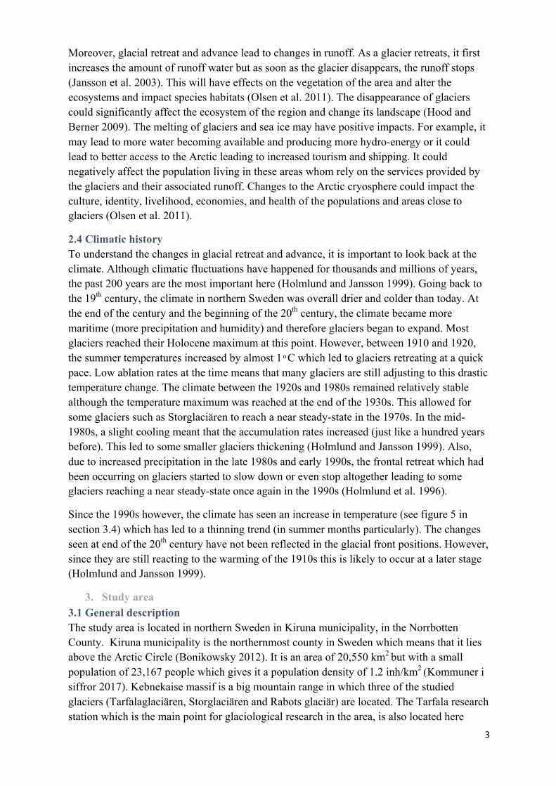
Figure 5: The average summer, winter and annual temperature at Tarfala climatological station. Data from the Bolin Centre for Climate Research, Tarfala research station database (retrieved 2017).

Almost no precipitation falls between January and April and the driest month is March (figure 6). Most precipitation falls from June until September (average of 7.5mm but can be up to 80mm) before it starts to level out again in October (Holmlund and Dyurgerov 2011).

Figure 6: The average monthly precipitation at Tarfala climatological station. Data from the Bolin Centre for Climate Research, Tarfala research station database (retrieved 2017).

Figure 7 shows the average precipitation changes in Tarfala from 1986-2011. As can be seen, the summer and winter precipitation have the same trend. The year 1991 received a very high amount of summer precipitation so it can be assumed that the winter precipitation was also high. Since 2005, the precipitation has increased overall although there is some variability from year to year.

-12,0

-10,0

-8,0

-6,0

-4,0

-2,0

0,0

2,0

4,0

6,0

8,0

1986 1991 1996 2001 2006 2011

Tempe

rature(ͦC)

Year

Temperaturetrends.1986-2011

Year Summer Winter

8

Figure 7: The average precipitation for the year, the summer months and the winter months for the period 1986-2011. Data from the Bolin Centre for Climate Research, Tarfala research station database (retrieved 2017).

Figure 8 shows the mean horizontal wind speed for each month during the year 2011. It is possible to see that the wind speeds are higher in winter than in summer. The mean maximum wind speed also follows the same pattern.

Figure 8: The average wind speed and the average maximum wind speed for 2011. Data from the Bolin Centre for Climate Research, Tarfala research station database (retrieved 2017).

Figure 9 shows the wind speed over the 15-year period. It can be seen that the winter average decreased between 1990 and 2005 but increased by 0.8 m/s between 2005 and 2011. The summer wind speed on the other hand has fluctuated a lot during the time-period but unlike

2,00

4,00

6,00

8,00

10,00

12,00

14,00

Windspeed(m

/s)

Monthoftheyear

Windspeeds(2011)

Meanhorizontalwindspeed Meanmaximunwindspeed

9

the winter average it decreased between 2005 and 2011. The mean annual wind speed has fluctuated although it has always stayed between 3.3- 3.7 m/s.

Figure 9: The average wind speed between 1990 and 2011. Data from the Bolin Centre for Climate Research, Tarfala research station database (retrieved 2017).

3.5 The glaciers The five glaciers studied are Tarfalaglaciären, Storglaciären, Riukojietna, Rabots glaciär, and Mårmaglaciären. Below is a brief description of the glaciers:

Tarfalaglaciären: This glacier is located on the eastern slope of a mountain called Tarfalatjakka (figure 3). It is a small glacier located at a high altitude and therefore receives a lot of accumulation. It has a very strong correlation with Storglaciären in terms of accumulation (0.97) and also for ablation (0.92) (Holmlund et al. 1996). The glacier is different from others since it is believed to be frozen to the bed which means that it is not capable of basal sliding unless it becomes thick enough to become wet at the base, something requires a huge amount of accumulation (Grudd 1990). Grudd (1990) also found that while other glaciers see changes in volume through frontal changes, Tarfalaglaciären sees most of its changes through thinning.

Figure 10: Tarfalaglaciären in 2014. Image taken by Per Holmlund. Glacier Photograph Collection, Boulder, Colorado, USA, National Snow and Ice Data Centre.

2,5

2,7

2,9

3,1

3,3

3,5

3,7

3,9

4,1

4,3

4,5

1990 1995 2000 2005 2011

Windspeed(m

/S)

Years

Meanhorizontalwindspeed(m/s)

Yearlyaverage Summeraverage Winteraverage

10

Storglaciären: It is the most studied glacier of all five and has the longest mass balance record in the world (1945 to present) (Holmlund and Jansson 1999). It has a 30-40m thick cold surface and many subglacial overdeepnings and ridges at the base. It receives a lot of accumulation due to the westerly winds. The glacier was close to reaching a steady state in the 1970s and the 1990s (Stroeven and al 1990). The fact that Storglaciären was very quick to react to the climate changes at the beginning of the 20th century and that it has reached a near steady state many times, infers that it is much more sensitive to climate changes than other glaciers. This is because of its fast ice velocities which derive from its steepness and ice thickness (Brugger et al. 2005). Storglaciären has been compared to the other glaciers in the area with less dense measurement readings and shorter time series to see if it is representative of the area (Stroeven and Wal 1990; Holmlund and Jansson 1999; Holmlund et al. 1996). It has been found that the mass balance of Storglaciären is representative of the area (Stroeven and Wal 1990; Holmlund and Jansson 1999; Rosqvist and Ostrem 1989).

Figure 11: Storglaciären in 2013. Image taken by Per Holmlund. Glacier Photograph Collection, Boulder, Colorado, USA, National Snow and Ice Data Centre.

Mårmaglaciären: It is quite similar to Storglaciären in terms of size, type, and aspect. It also has a thick cold surface layer, just like Storglaciären except that this one is much thicker and colder. Compared to the glaciers, it is in a more continental climate due to being located east of several high mountains which means that it receives less accumulation than the other studied glaciers (Holmlund and Jansson 1999).

Figure 12: Mårmaglaciären in 2011. Image taken by Per Holmlund. Glacier Photograph Collection, Boulder, Colorado, USA, National Snow and Ice Data Centre.

11

Riukojietna: It is a small ice cap on the Swedish-Norwegian border. Of all the glaciers, it is the closest to the coast and therefore has a much more maritime climate; however, it obtains less accumulation than Storglaciären due to its low elevation (Holmlund and Jansson 1999). As table 1 shows, it is situated on a plateau at 1456-1130 m.a.s.l but the mountains surrounding the glacier reach elevations of 1600m (Rosqvist and Ostrem 1989). Riukojietna also used to cover a lake in the 1960s which means that calving used to be a significant factor in the ablation balance. However, since 1978 the glacier has retreated which means that it no longer terminates at the lake (Rosqvist and Ostrem 1989).

Figure 13: Riukojietna in 2014. Images taken by Per Holmlund. Glacier Photograph Collection, Boulder, Colorado, USA, National Snow and Ice Data Centre.

Rabots glaciär: This glacier is situated very close to Storglaciären and has the second longest mass balance record (1982 to present). Unlike the other glaciers, it has three accumulation areas which all lead to a common ablation area. It is flatter than Storglaciären around the equilibrium line which is where 80% of the surface area can be found. Due to being west of the massif, it is directly exposed to the prevailing westerly winds (Stroeven and Wal 1990). It is unique because it has a high north-facing wall which means that parts of the glacier are almost always in the shadow and therefore do not experience as much ablation as other parts of the glacier. This means that it has a strong lateral gradient and that there is a poor correlation between ablation and elevation (Holmlund and Jansson 1999; Brugger et al 2005). Rabots glaciär has a slow response time to climate change which means that it is still responding to the climatic changes at the beginning of the 20th century. It is out of balance with the current climate (Holmlund and Jansson 1999; Brugger et al. 2005, Brugger 2007).

12

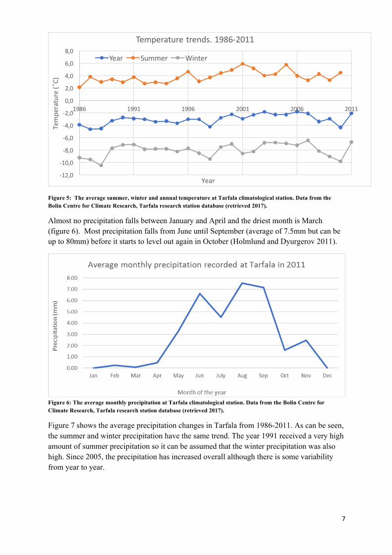
Figure 14: Rabots glaciär in 2011. Images taken by Per Holmlund. Glacier Photograph Collection, Boulder, Colorado, USA, National Snow and Ice Data Centre.

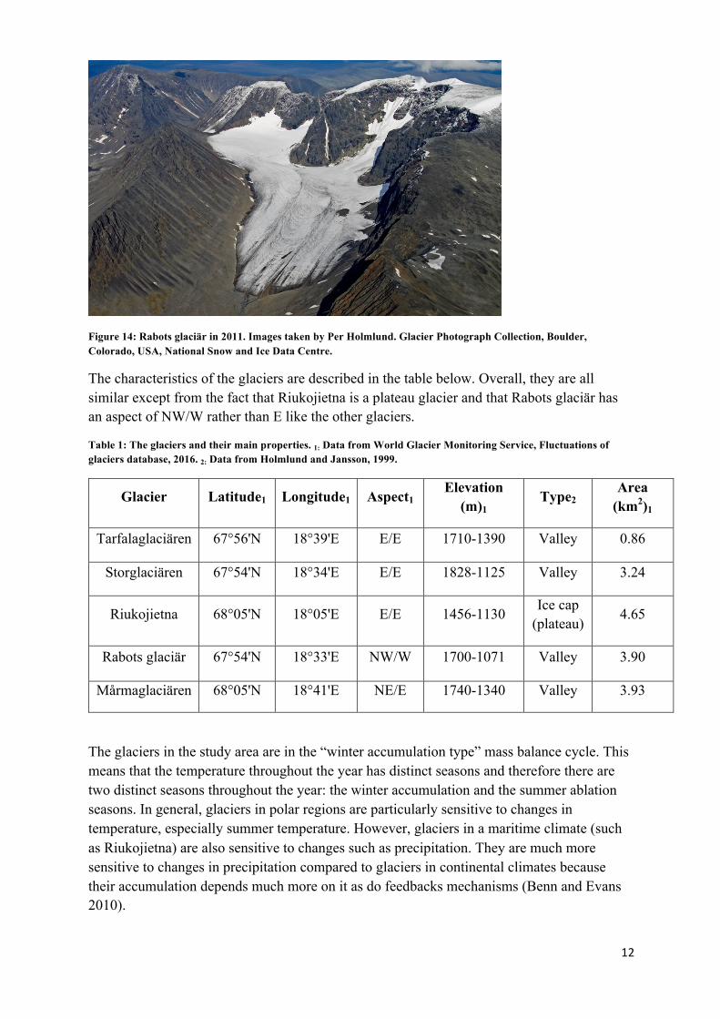
The characteristics of the glaciers are described in the table below. Overall, they are all similar except from the fact that Riukojietna is a plateau glacier and that Rabots glaciär has an aspect of NW/W rather than E like the other glaciers.

Table 1: The glaciers and their main properties. 1: Data from World Glacier Monitoring Service, Fluctuations of glaciers database, 2016. 2: Data from Holmlund and Jansson, 1999.

Glacier Latitude1 Longitude1 Aspect1 Elevation

(m)1 Type2

Area (km2)1

Tarfalaglaciären 67°56'N 18°39'E E/E 1710-1390 Valley 0.86

Storglaciären 67°54'N 18°34'E E/E 1828-1125 Valley 3.24

Riukojietna 68°05'N 18°05'E E/E 1456-1130 Ice cap (plateau)

4.65

Rabots glaciär 67°54'N 18°33'E NW/W 1700-1071 Valley 3.90

Mårmaglaciären 68°05'N 18°41'E NE/E 1740-1340 Valley 3.93

The glaciers in the study area are in the “winter accumulation type” mass balance cycle. This means that the temperature throughout the year has distinct seasons and therefore there are two distinct seasons throughout the year: the winter accumulation and the summer ablation seasons. In general, glaciers in polar regions are particularly sensitive to changes in temperature, especially summer temperature. However, glaciers in a maritime climate (such as Riukojietna) are also sensitive to changes such as precipitation. They are much more sensitive to changes in precipitation compared to glaciers in continental climates because their accumulation depends much more on it as do feedbacks mechanisms (Benn and Evans 2010).

13

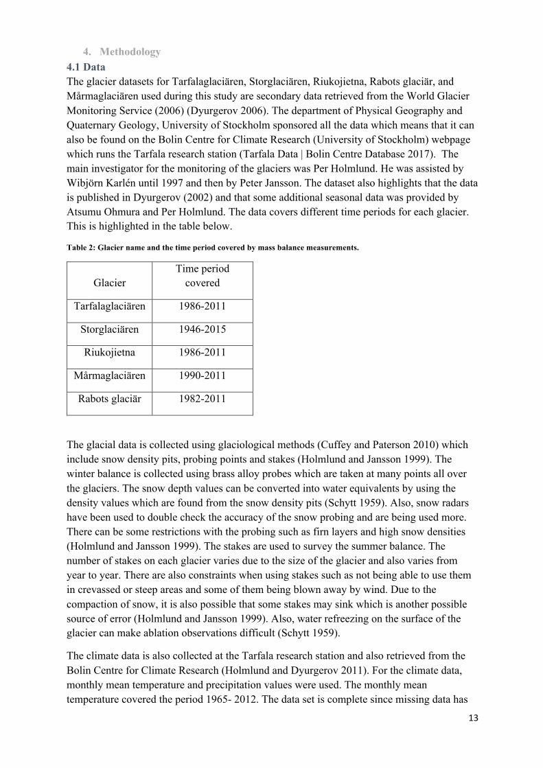
4. Methodology 4.1 Data The glacier datasets for Tarfalaglaciären, Storglaciären, Riukojietna, Rabots glaciär, and Mårmaglaciären used during this study are secondary data retrieved from the World Glacier Monitoring Service (2006) (Dyurgerov 2006). The department of Physical Geography and Quaternary Geology, University of Stockholm sponsored all the data which means that it can also be found on the Bolin Centre for Climate Research (University of Stockholm) webpage which runs the Tarfala research station (Tarfala Data | Bolin Centre Database 2017). The main investigator for the monitoring of the glaciers was Per Holmlund. He was assisted by Wibjörn Karlén until 1997 and then by Peter Jansson. The dataset also highlights that the data is published in Dyurgerov (2002) and that some additional seasonal data was provided by Atsumu Ohmura and Per Holmlund. The data covers different time periods for each glacier. This is highlighted in the table below.

Table 2: Glacier name and the time period covered by mass balance measurements.

Glacier Time period

covered

Tarfalaglaciären 1986-2011

Storglaciären 1946-2015

Riukojietna 1986-2011

Mårmaglaciären 1990-2011

Rabots glaciär 1982-2011

The glacial data is collected using glaciological methods (Cuffey and Paterson 2010) which include snow density pits, probing points and stakes (Holmlund and Jansson 1999). The winter balance is collected using brass alloy probes which are taken at many points all over the glaciers. The snow depth values can be converted into water equivalents by using the density values which are found from the snow density pits (Schytt 1959). Also, snow radars have been used to double check the accuracy of the snow probing and are being used more. There can be some restrictions with the probing such as firn layers and high snow densities (Holmlund and Jansson 1999). The stakes are used to survey the summer balance. The number of stakes on each glacier varies due to the size of the glacier and also varies from year to year. There are also constraints when using stakes such as not being able to use them in crevassed or steep areas and some of them being blown away by wind. Due to the compaction of snow, it is also possible that some stakes may sink which is another possible source of error (Holmlund and Jansson 1999). Also, water refreezing on the surface of the glacier can make ablation observations difficult (Schytt 1959).

The climate data is also collected at the Tarfala research station and also retrieved from the Bolin Centre for Climate Research (Holmlund and Dyurgerov 2011). For the climate data, monthly mean temperature and precipitation values were used. The monthly mean temperature covered the period 1965- 2012. The data set is complete since missing data has

14

been filled. A complete data set for precipitation which covered the whole year is available for 1998-2011 but data covering only the summer months are available as early as 1980.

The climate data was collected using a computer-based automatic climate station which was installed in 1988. The equipment used is a Campbell Scientific datalogger. It has sensors which record air temperature, humidity, precipitation, wind speed and direction, net radiation and incoming radiation. The datalogger takes measurements every ten seconds and stores mean values every hour between May and September (summer months) and every three hours between October and April (winter months). It also records the daily maximum, minimum and mean. The station has seen some upgrades such as installing a Pt100 sensor to measure the stability of the temperature values (Grudd and Schneider 1996). Since the mid-1990s, the station has been upgraded and some pieces of equipment have been added. Table 3 gives an overview of which pieces of equipment were used on the climate station in 2011 (Jansson 2011).

Table 3: The equipment used at the climate station at Tarfala (Jansson 2011).

Sensor Remark

Pt 100 In Stevenson screen

Pt 100 In Young screen

Young Wind Monitro At 3m

LiCor Li-200SB pyranometer At 2m

Tipping bucket precipitation gauge At 2m

Vent HygroClip T/Rh At 2m

CR10X-2M data logger

4.2 Data preparation Once all the data for the glaciers had been downloaded and uploaded into an Excel workbook, the summer, winter, and net mass balance for all glaciers were assembled and plotted into graphs. It must be pointed out that although data dating back to 1946 are available, only the data between 1986 and 2011 were used in order to ensure a fair comparison between all parameters. The summer months’ count May, June, July, August and September while the winter months are October through to April. This means that it is possible to see the trends in the parameters over time. The same was done for the climate data (temperature, precipitation, and wind). These graphs allowed for an overview of the climate through the 15-year period and also throughout the year. It must be pointed out that the time series for the winter, summer, and net mass balance cover 1986-2011 whilst the ELA data cover 2001-2011 due to limited and missing data. Also, although the data have been filled as much as possible, there are still missing data which is why some graphs may look incomplete.

15

4.3 Statistical analyses In order to find which parameters affected the mass balance and the equilibrium line altitude the most, statistical analyses were carried out.

First, trend lines were added to the graphs made in Microsoft Excel in order to see the overall trends of the glaciers. To do this, the average winter, summer and net mass balances were calculated and a trend line was added onto the graphs. The linear equation and the r-squared value of the average trend are displayed on the graphs. This was not done for the ELA since the trends among the glaciers were too erratic.

The programme IBM SPSS ® was used to carry out a F-test (ANOVA) to find if the summer, winter, and net mass balances and ELAs of all the glaciers came from the same population which would show if they differed significantly from one another or not. An ANOVA test (analysis of variance) is used to determine the equality of variances of different samples. This means that it is possible to see if the samples all come from the same populations or not (if they differ too much). It is a ratio between the variation between sample means and between variation within sample (Frost 2017). This test was chosen as it would assess whether the glaciers all came from the same population. The full equations for this can be found in the appendix. The actual step-by-step procedure for this test can also be found in the appendix.

The programme was also used to find the R2 values and the significance level (p-values) between the climate and the glacial variables. The R2 is a Persson correlation which reveals how much of the variation in the summer, winter, net mass balances and ELAs can be attributed to the climate. This means that it is possible to find differences within the glaciers and therefore reasons for different trends. The significance level also shows how trusted the results are. For the results to be significance they must have a p-value lower than 0.05.

5. Results 5.1 Winter mass balance The winter mass balance shows how much accumulation has occurred on the glacier and therefore how much mass has been gained during the winter season (Cuffey and Paterson 2010). These numbers are positive since they represent gain. Figure 15 shows that all glaciers show similar patterns over the years with a slight increase in the late 80s, reaching a maximum in 1989, meaning that there was more accumulation. Then, the winter balance started to decrease and has had the same general pattern since with some natural fluctuations from year to year.

All glaciers had a lower winter balance in 2011 than in 1986 except for Riukojietna which saw a huge increase between 2010 and 2011 from 0.63 m.w.eq to 1.69 m.w.eq. In fact, all the glaciers saw an increase in winter balance between 2010 and 2011 except for Rabots glaciär which continued to decrease.

Over the 15 year period, it is the Tarfalaglaciären which has decreased the most in winter balance with a difference of 1.02 m.w.eq whereas Mårmaglaciären saw the smallest change of just 0.32 m.w.eq. Riukojietna actually had a negative difference (so winter balance increasing over the time period) of -0.46 m.w.eq. These differences do not include the maximum and minimum values observed during the time period but merely show the net difference over 15 years.

16

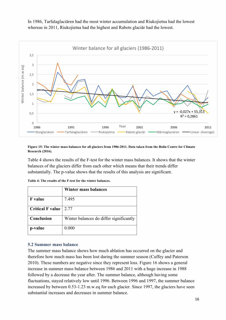
In 1986, Tarfalaglaciären had the most winter accumulation and Riukojietna had the lowest whereas in 2011, Riukojietna had the highest and Rabots glaciär had the lowest.

Figure 15: The winter mass balances for all glaciers from 1986-2011. Data taken from the Bolin Centre for Climate Research (2016).

Table 4 shows the results of the F-test for the winter mass balances. It shows that the winter balances of the glaciers differ from each other which means that their trends differ substantially. The p-value shows that the results of this analysis are significant.

Table 4: The results of the F-test for the winter balances.

Winter mass balances

F value 7.495

Critical F value 2.77

Conclusion Winter balances do differ significantly

p-value 0.000

5.2 Summer mass balance The summer mass balance shows how much ablation has occurred on the glacier and therefore how much mass has been lost during the summer season (Cuffey and Paterson 2010). These numbers are negative since they represent loss. Figure 16 shows a general increase in summer mass balance between 1986 and 2011 with a huge increase in 1988 followed by a decrease the year after. The summer balance, although having some fluctuations, stayed relatively low until 1996. Between 1996 and 1997, the summer balance increased by between 0.53-1.23 m.w.eq for each glacier. Since 1997, the glaciers have seen substantial increases and decreases in summer balance.

y=-0,027x+55,313R²=0,2861

0

0,5

1

1,5

2

2,5

3

3,5

1986 1991 1996 2001 2006 2011

Winterb

alance(m

.w.eq)

Year

Winterbalanceforallglaciers(1986-2011)

Storglaciären Tarfalaglaciären Riukojietna Rabotsglaciär Mårmaglaciären Linear(Average)

17

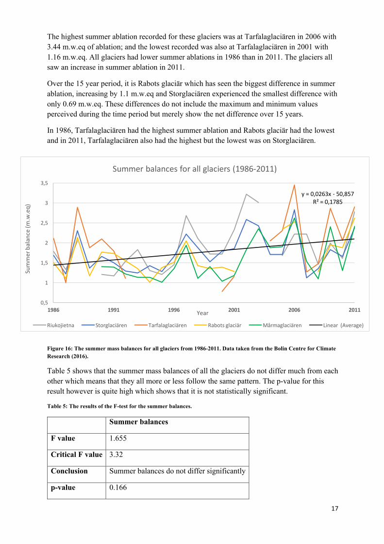
The highest summer ablation recorded for these glaciers was at Tarfalaglaciären in 2006 with 3.44 m.w.eq of ablation; and the lowest recorded was also at Tarfalaglaciären in 2001 with 1.16 m.w.eq. All glaciers had lower summer ablations in 1986 than in 2011. The glaciers all saw an increase in summer ablation in 2011.

Over the 15 year period, it is Rabots glaciär which has seen the biggest difference in summer ablation, increasing by 1.1 m.w.eq and Storglaciären experienced the smallest difference with only 0.69 m.w.eq. These differences do not include the maximum and minimum values perceived during the time period but merely show the net difference over 15 years.

In 1986, Tarfalaglaciären had the highest summer ablation and Rabots glaciär had the lowest and in 2011, Tarfalaglaciären also had the highest but the lowest was on Storglaciären.

Figure 16: The summer mass balances for all glaciers from 1986-2011. Data taken from the Bolin Centre for Climate Research (2016).

Table 5 shows that the summer mass balances of all the glaciers do not differ much from each other which means that they all more or less follow the same pattern. The p-value for this result however is quite high which shows that it is not statistically significant.

Table 5: The results of the F-test for the summer balances.

Summer balances

F value 1.655


Conclusion Summer balances do not differ significantly

p-value 0.166

y=0,0263x- 50,857R²=0,1785

0,5

1

1,5

2

2,5

3

3,5

1986 1991 1996 2001 2006 2011

Summerbalance(m

.w.eq)

Year

Summerbalancesforallglaciers(1986-2011)

Riukojietna Storglaciären Tarfalaglaciären Rabotsglaciär Mårmaglaciären Linear(Average)

18

5.3 Net mass balance The net mass balance of a glacier is the accumulation minus the ablation which shows whether a glacier is losing or gaining mass during a one-year period. A positive value shows that accumulation is bigger than ablation and therefore the glacier is gaining mass but a negative value shows that the glacier is losing mass (Cuffey and Paterson 2010).

Figure 17 shows a general decreasing trend in net mass balance for all glaciers. In 1986 none of the glaciers had positive mass balances. However, this changed in 1987 but the net mass balances dropped massively in 1988. By 1989, the mass balances for all the glaciers were positive again (three glaciers experienced their maximum mass balance). By 1990, however, the mass balance had decreased again and until 2006 this trend continued with normal fluctuations over time. In 2006, the glaciers reached a new minimum although in 2007 and 2008 the mass balance had increased to be positive again. This was a huge increase, especially for Tarfalaglaciären which experienced an increase in mass balance of 2.13 m.w.eq in one year. After 2008 though, the mass balance has been decreasing again. Overall, the mass balance for all glaciers were lower in 2011 than in 1986 which shows a loss of mass.

The highest mass balance recorded was in 1992 for Tarfalaglaciären with a mass balance of 1.36 m.w.eq and the lowest was also for Tarfalaglaciären in 2006 with -2.53 m.w.eq. Tarfalaglaciären had more extreme values than the other glaciers, particularly in 2000 and 2001 with a positive mass balance whilst all the other glaciers had negative values. Riukojietna also stands out between 1997-2003 for having much lower mass balance values than any other glacier.

Over the 15 year time period, it was Rabots glaciär which had the biggest overall change in net mass balance, with a difference of 2.31 m.w.eq between 1986 and 2011. Storglaciären, on the other hand had the smallest difference with just 1.06 m.w.eq between 1986 and 2011. As already mentioned above, the values do not include the maximum and minimum values during the time but just show the net difference over 15 years.

19

In 1986, Tarfalaglaciären had the highest mass balance and Riukojietna had the lowest but by 2011 it was Storglaciären which had the highest and Rabots glaciär which had the lowest.

Figure 17: The net mass balances for all glaciers from 1986-2011. Data taken from the Bolin Centre for Climate Research (2016).

It can be seen from table 6 that the net mass balances of all the glaciers do not differ much from each other, just like the summer balance. However, the p-value is even higher than with the summer balance so this result is not statically relevant.

Table 6: The results of the F-test for the net mass balances.

Net mass balances

F value 1.177


Conclusion Net mass balances do not differ significantly

p-value 0.325

5.4 Equilibrium line altitude The equilibrium line altitude shows the separation between the accumulation and ablation zones (summer and winter balances) and it can thus be used as a proxy for determining if a glacier is advancing or retreating. An increasing ELA suggests that the glacier is retreating while a decreasing ELA suggests that the glacier is advancing (Cuffey and Paterson 2010).

As can be seen from figure 18, the glaciers show different trends with time. Whilst, the ELA for Tarfalaglaciären and Riukojietna seem to be decreasing in altitude, the ELA for Storglaciären, Rabots glaciär and Mårmaglaciären seem to be increasing.

y=-0,0531x+105,7R²=0,35189

-2,6

-2,1

-1,6

-1,1

-0,6

-0,1

0,4

0,9

1,4

1986 1991 1996 2001 2006 2011

Netm

assb

alance(m

.w.eq)

Year

Netmassbalanceforallglaciers(1986-2011)

Storglaciären Tarfalaglaciären Riukojietna Rabotsglaciär Mårmaglaciären Linear(Average)

20

Tarfalaglaciären has the biggest variations over time and also the biggest advance. It first increases to 1790m in 2005 and 2006 before decreasing to 1475m in 2007. It then increased back up to 1790m in 2009 and 2010 but had its lowest ELA in 2011 at 1390m which is a huge difference of 400m compared to previous years.

Rabots glaciär on the other hand, saw a huge increase between 2008 and 2011 where it increased 600m from 1380m to 1930m. The biggest proportion of the increase took place between 2010 and 2011 (increase of 260m) which shows a retreat of the glacier.

Mårmaglaciären is the glacier with the least variation over time with its first ELA recording being at 1643m in 2001 and its latest being at 1660m in 2011. It did experience a slight advance in 2005 when it reached 1525m.

Figure 18: The ELA for all glaciers from 2001 to 2011. Data taken from the Bolin Centre for Climate Research (2016).

Just like the winter balance, the trends of the ELAs of all the glaciers do differ from one another (table 7). The significance of this result is very high (0.01) which means that the result is statistically significant.

Table 7: The results of the F-test for the equilibrium line altitudes.

ELA

F value 6.239

Critical F value 1

Conclusion ELAs do differ significantly

p-value 0.01

1350

1450

1550

1650

1750

1850

1950

2000 2002 2004 2006 2008 2010 2012

ELA(m

.a.s.l)

Year

Equilibriumlinealtitude

Riukojietna Storglaciären Tarfalaglaciären Rabotsglaciär Mårmaglaciären

21

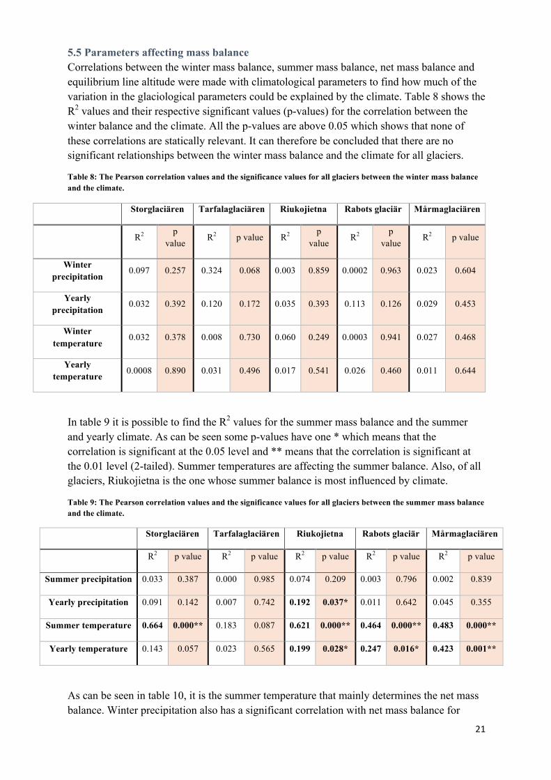
5.5 Parameters affecting mass balance Correlations between the winter mass balance, summer mass balance, net mass balance and equilibrium line altitude were made with climatological parameters to find how much of the variation in the glaciological parameters could be explained by the climate. Table 8 shows the R2 values and their respective significant values (p-values) for the correlation between the winter balance and the climate. All the p-values are above 0.05 which shows that none of these correlations are statically relevant. It can therefore be concluded that there are no significant relationships between the winter mass balance and the climate for all glaciers.

Table 8: The Pearson correlation values and the significance values for all glaciers between the winter mass balance and the climate.

Storglaciären Tarfalaglaciären Riukojietna Rabots glaciär Mårmaglaciären

R2 p value

R2 p value R2 p value

R2 p value

R2 p value

Winter precipitation

0.097 0.257 0.324 0.068 0.003 0.859 0.0002 0.963 0.023 0.604

Yearly precipitation

0.032 0.392 0.120 0.172 0.035 0.393 0.113 0.126 0.029 0.453

Winter temperature

0.032 0.378 0.008 0.730 0.060 0.249 0.0003 0.941 0.027 0.468

Yearly temperature 0.0008 0.890 0.031 0.496 0.017 0.541 0.026 0.460 0.011 0.644

In table 9 it is possible to find the R2 values for the summer mass balance and the summer and yearly climate. As can be seen some p-values have one * which means that the correlation is significant at the 0.05 level and ** means that the correlation is significant at the 0.01 level (2-tailed). Summer temperatures are affecting the summer balance. Also, of all glaciers, Riukojietna is the one whose summer balance is most influenced by climate.

Table 9: The Pearson correlation values and the significance values for all glaciers between the summer mass balance and the climate.


R2 p value R2 p value R2 p value R2 p value R2 p value

Summer precipitation 0.033 0.387 0.000 0.985 0.074 0.209 0.003 0.796 0.002 0.839

Yearly precipitation 0.091 0.142 0.007 0.742 0.192 0.037* 0.011 0.642 0.045 0.355

Summer temperature 0.664 0.000** 0.183 0.087 0.621 0.000** 0.464 0.000** 0.483 0.000**

Yearly temperature 0.143 0.057 0.023 0.565 0.199 0.028* 0.247 0.016* 0.423 0.001**

As can be seen in table 10, it is the summer temperature that mainly determines the net mass balance. Winter precipitation also has a significant correlation with net mass balance for

22

Storglaciären and Tarfalaglaciären. Riukojietna is also affected by the yearly precipitation. On the other hand, Rabots glaciär and Mårmaglaciären are affected by the yearly temperature.

Table 10: The Pearson correlation values and the significance values for all glaciers between the net mass balance and the climate.



Summer precipitation 0.442 0.665 0.004 0.803 0.068 0.218 0.0001 0.956 0.005 0.772

Winter precipitation 0.270 0.047* 0.404 0.035* 0.237 0.077 0.097 0.325 0.102 0.267

Yearly precipitation 0.027 0.164 0.059 0.344 0.223 0.020* 0.065 0.252 0.063 0.273

Summer temperature 0.469 0.000** 0.347 0.013* 0.546 0.000** 0.482 0.000** 0.411 0.001**

Winter temperature 0.013 0.573 0.010 0.704 0.008 0.678 0.019 0.525 0.036 0.398

Yearly temperature 0.045 0.213 0.203 0.451 0.090 0.146 0.179 0.044* 0.303 0.008**

Table 11 shows that the correlations between the equilibrium line altitude and climate are much weaker and there is no significance. There is an exception with Riukoiietna and Rabots glaciär where there is a significant correlation between the ELA and the summer precipitation.

Table 11: The Pearson correlation values and the significance values for all glaciers between equilibrium line altitude and the climate.

6. Discussion 6.1 Summer and winter mass balances The results section showed the trends for all glaciers. It was possible to see that between 1986 and 2011 the winter balance decreased and the summer balance increased. This means that the accumulation of glaciers decreased and the ablation increased which is reflected in the net



Summer precipitation 0.021 0.672 0.125 0.391 0.486 0.025* 0.576 0.048* 0.297 0.103

Winter precipitation 0.046 0.526 0.331 0.136 0.088 0.404 0.019 0.767 0.021 0.687

Yearly precipitation 0.028 0.625 0.100 0.444 0.378 0.058 0.551 0.056 0.222 0.170

Summer temperature 0.228 0.138 0.026 0.704 0.101 0.370 0.031 0.704 0.207 0.187

Winter temperature 0.005 0.831 0.340 0.129 0.077 0.437 0.141 0.407 0.007 0.813

Yearly temperature 0.068 0.439 0.123 0.395 0.006 0.833 0.075 0.553 0.018 0.715

23

mass balance which has shown a shift to a more negative mass balance (glaciers are losing more and more mass overall). One reflection is that the summer balance is much more fluctuating and variable than the winter balance (figure 15 and 16) and therefore must be much more sensitive to the changing climate. This was also observed by Holmlund and Jansson (1999) whom pointed out that the summer ablation depends on summer temperatures which vary a lot (figure 5). Another reflection, is that in the late 1980s and early 1990s, the winter balance actually increased meaning that glaciers put on more mass (figure 15). This is the time when some glaciers started to adapt to the 1910s change in climate in which the temperature decreased and precipitation increased so more accumulation was possible (Holmlund and Jansson 1999).

When looking at the winter balance, the main difference which can be seen between all the glaciers is that during the 15-year period, Riukojietna overall had an increase in winter accumulation, whereas all other glaciers had a decrease. However, this apparent increase was due to a big increase from 2010 to 2011. When considering the trend overall, it can be seen that Riukojietna fluctuates a lot but does not have an increasing trend. Its accumulation is always lower than Storglaciären and Tarfalaglaciären. This is because although Riukojietna is situated closer to the coast and is exposed to a more maritime climate and should thus receive more precipitation (Cuffey and Paterson 2012); it is situated at a low elevation (1450-1130 m.a.s.l) and therefore receives less accumulation.

The results of the F-test showed that the winter balance trends did differ significantly one from another which means that all the glaciers have different trends. This can be explained by the differences in location, aspect and elevation of the glaciers. For example, Riukojietna is located at lower elevations and so receives less accumulation; Rabots glaciär is located on the western side of the Kebnekaise massif and has an aspect of NW/W so it receives less accumulation than Storglaciären. Storglaciären has the most accumulation due to being on the lee side of the mountain massif thus receiving leeward deposition and more precipitation as air masses pass over Kebnekaise (Holmlund and Jansson 1999). Mårmaglaciären is located to the eastern side of the massif and so has more of a continental climate which obtains less accumulation.

Unlike the winter balance, the summer balance seems to show the same trend for all glaciers (however this result was not statically significant, table 5). There were much more extreme values such as Riukojietna for example, which experienced much higher ablation between 1997 and 2003. This can be attributed to the fact that Riukojietna is situated at a much lower elevation (1450-1130 m.a.s.l compared to 1740-1340 m.a.sl. for Mårmaglaciären) than all the other glaciers and therefore reaches higher temperatures, especially during summer and therefore is prone to higher ablation rates. Also, Stroeven and Wal (1990) stated that glaciers with low accumulation rates such as Riukojietna will enhance melting because of a quick albedo decrease in April/May (early summer). Furthermore, Holmlund et al (1996) pointed out that at high altitudes the radiation is a much more important controlling factor, whereas at lower elevations (such as Riukojietna), it is advection which is much more important due to humidity. The fact that Rabots glaciärs’ summer balance does not differ so much from the other glaciers (see F-test in table 5) although it has a different aspect suggests that aspect is not so important for ablation. However, the result of this F-test was statistically insignificant and therefore should not be considered to be meaningful.

24

6.2 Net mass balance The glaciers studied here are non-surging glaciers which means that the glacier fluctuations observed are due to changes in mass balance. The mass balance of these glaciers is controlled by air temperature, precipitation, radiation absorption, condensation and evaporation. Condensation and evaporation are controlled by humidity and wind speed which can be of high importance (Rosqvist and Ostrem 1989).

The net mass balance shows that all the glaciers have the same overall trend of the mass balance becoming more negative during the 15-year period (table 6, not statistically significant). Nevertheless, a few values in particular can be pointed out. Tarfalaglaciären had a very positive mass balance in 1991 and 2000 compared to all the other glaciers (up to 1.4 m.w.eq compared to 0.5 m.w.eq) and also a very negative mass balance in 2006 (-2.6 m.w.eq compared to -0.6 m.w.eq). The former can be explained by its high altitude which means that it receives a lot of precipitation as snow. The high ablation rates can be explained by the summer radiation which is a major contributing factor for ablation at high altitudes (Holmlund et al. 1996). When looking at the whole time series, Tarfalaglaciären has much more extreme values than all other glaciers which suggest that it is particularly sensitive to changes in climate which is explained by its location. It is the only glacier in Kebnekaise which is not located in a deep cirque, but it lies on the highest slope of Tarfalatjakko which is smooth and gentle (Schytt 1959). This means that it is much more exposed to winds, radiation, deposition and sublimation.

Riukojietna also showed some extreme values between 1997 and 2006 where its mass balance was significantly lower than the other glaciers which suggests that it was losing mass at a much quicker rate than all other glaciers. As already discussed above, this was due to its low elevation. It must be pointed out however, that Riukojietna had one of the smallest overall changes in net mass balance between 1986-2011 and this might be attributed to the fact that it is an ice cap and it therefore does not cover a large vertical gradient and so is not prone to big changes in elevation and hence climate.

On the other hand, Storglaciären had the least change but it has had many extreme values in net mass balance over the 15 years. These extreme values could be due to it being the longest glacier and it covering elevations between 1830-1125 m.a.s.l. This means that it experiences high temperatures at low elevations (just like Riukojietna) which leads to high ablation rates. The high accumulation rates are due to the high altitude such as 1800 m.a.s.l which means that Storglaciären receives a lot of precipitation in the form of snow rather than rain. It must be noted that Storglaciären is situated on the eastern rim of the Kebnekaise massif which means that the moist winds coming from the west which are then lifted over the massif produce orographic precipitation onto the glacier which is why it receives high accumulation rates compared to Rabots glaciär (Stroeven and Wal 1990, Holmlund and Jansson 1999). Also, Storglaciären is a glacier which reached a near steady-state in the 1990s which suggests that it was in balance with the climate at the beginning of the century. However, with the recent climatic changes, the glaciers are now once again changing and since Storglaciären is such a big glacier, the changes could be seen in a few decades which means that it will not reach a steady state for a while (Stroeven and al 1990, Cuffey and Paterson 2010).

25

Another observation is that during the time period, it was Rabots glaciär which had the biggest overall change (particularly between 2008 and 2011). When looking at figure 15 and 16 it is obvious that this change is due to big changes in summer ablation. The fact that it is located on the western rim of the massif means that it is directly exposed to the westerly winds which could lead to higher rates of melting (Field unpublished). Also, unlike all the other glaciers, Rabots glaciär has an aspect of NW/W which once again directly exposes it to strong winds. Strong winds, a warm surface and dry air can all increase sublimation (Cuffey and Paterson 2012). These factors could all occur on Rabots glaciär, particularly with a NW/W orientation which is why the summer ablation has been increasing (particularly with the increasing air temperatures).

Even though Rabots glaciär and Storglaciären have similar elevations, lengths, and locations; Rabots glaciärs’ response time is much slower than Storglaciären. Brugger et al (2005) explained that this was because the ice velocities on Storglaciären were much faster than on Rabots glaciär due to Storglaciären being steeper and having greater ice thickness in the accumulation area whilst Rabots is flatter. In fact, Rabots glaciärs’ thickness is pretty uniform, as in 2003 much of the glacier was about 85m thick with the thickest part being 175m. This proves that ice thickness and steepness can affect how quickly a glacier can respond to changes in climate. Just like the summer balance, the F-test (table 6) indicates that the net mass balance trends of the glaciers did not differ significantly from one another. This shows that the changes in climate have affected the glaciers in similar ways, regardless of elevation, aspect and location. Perhaps, it is the summer mass balance which affects the net mass balance more than the winter balance. Benn and Evans (2010) stated that it was winter precipitation and summer temperature which affected the net mass balance the most but as table 10 showed, there are only two significant relationships between the winter precipitation and the net mass balance whereas summer temperature clearly has more of an effect since it has significant relationships for all the glaciers.

6.3 Equilibrium line altitude The ELA is a useful tool to see the changes in accumulation and ablation. The ELA for the glaciers are completely different and follow different trends (figure 18) but they all lower in 2003 which can be explained by an increase in accumulation (figure 15). Riukojietna had almost no change at all during the 10 years except from a lowering in 2010 which means that it started to advance again. This can be explained by the fact that it is a small ice cap and therefore extends over a plateau and thus is more prone to thickness changes rather than changes in length.

Mårmaglaciären also had almost no variation and remained stable except from the decrease in 2003. This can be attributed to the fact that Mårmaglaciären is situated east of the mountain range and is therefore in a continental climate which means that it is much more shielded and does not receive strong winds or big precipitation depositions. Storglaciären shows a very simple trend of decreasing ELA (and therefore bigger accumulation zone) between 2006-2008 and an increase since then (and therefore a smaller accumulation zone). This follows the pattern set out by the net mass balance (figure 17).

26

Rabots glaciär has a very fluctuating ELA. It sees an increase in the accumulation area between 2003 and 2008 and a huge decrease between 2009 and 2011 which proves that in recent years the glacier has experienced more ablation and less accumulation. Figure 17 shows that this change in ELA follows changes in net mass balance which are caused by changes in summer ablation. The reasons for these changes have already been mentioned. However, the fact that Rabots glaciär has a unique relationship between ablation, accumulation and net mass balance and elevation can be explained by its shading from Kebnekaise. Rabots glaciär is unique in the sense that it has a strong lateral gradient in accumulation and ablation due to shading from the Kebnekaise Mountain. The steep southern wall produces a shadow which means more accumulation and less ablation while the gently sloping northern wall does not produce a shadow which results in less accumulation and more ablation (Holmlund and Jansson 1999)

Tarfalaglaciären has the most unstable ELA. The main observation is the huge decrease between 2010 and 2011 which shows that the accumulation area became bigger by 400m. This trend is not represented in the net mass balance (figure 17) which actually shows a decrease in net mass balance between 2010 and 2011. The reason for this is that as mentioned in the background section, this glacier does not lose mass through frontal changes but through thinning which means that instead of the glacier advancing or retreating, its thickness changes.

The result of the F-test showed that the ELAs of the glaciers did differ significantly from each other (this result is statistically significant). Although they all had similar trends in net mass balance, their response to it in terms of changes in the accumulation/ablation balance proves that the changes in net mass balance can be represented in different ways. It is possible that changes in net mass balance may also be seen through changes in size and shape of the glacier, in the thickness of the glacier or in a reduction of the accumulation area from the highest elevation.

6.4 Parameters affecting mass balance. Although it would be expected that the variability in the winter mass balance would be due to winter precipitation (Benn and Evans 2010), table 11 shows that no significant variability in winter mass balance can be attributed to the winter or yearly climate for the study period. This means that the variability in winter mass balance must be due to another factor such as wind, humidity, moisture content or one of these factors in combination with one climatic factor too.

Table 9 is different as it clearly shows that summer mass balance has a strong significant variability caused by the summer temperature (46-66%) which proves that the summer ablation is dependent on the summer temperature. This is not true for Tarfalaglaciären however, which shows insignificant relationship. Riukojietna does have very strong relationships between the summer mass balance and the yearly precipitation (49%), summer temperature (62%) and yearly temperature (20%) which show that it is much more reliant on climate. The precipitation and temperature over the whole glacier is similar due to not having a large vertical gradient which means that the summer ablation is similar over the whole glacier (Rosqvist and Ostrem 1989).

27

When it comes to the net mass balance, the R2 values show that some of the variability can be attributed to the summer temperature (35-55%) for all glaciers which once again proves that the net mass balance depends on summer temperature. The other significant relationships differ for every glacier. For example, Rabots glaciär and Mårmaglaciären also depend on yearly temperature for net mass balance (18% and 30% respectively). This suggests that the temperatures throughout the year at these two glaciers are very important. The yearly temperature could potentially decide in which form the precipitation falls onto the glacier which ultimately decides if the precipitation will lead to more accumulation (snow) or if it will lead to more ablation (rain) (Cuffey and Paterson 2010). Tarfalaglaciären and Storglaciären’s net mass balance variability can be explained by summer temperature and also by winter precipitation (27% and 40% respectively) which reflects the most common view that net mass balance is controlled by summer temperature and winter precipitation (Benn and Evans 2010). However, Benn and Evans did state that winter precipitation would be more significant for glaciers located in maritime climates which Tarfalaglaciären and Storglaciären are not. Riukojietna however, is slightly different since it has a significant correlation with summer temperature but also with yearly precipitation (accounts for 22% of the variability) which suggests that contrary to its fellow glaciers, Riukojietna depends on all year-round precipitation rather than just the winter one. As already mentioned this is because of its gentle slopes which mean that it is much more sensitive to changes in climate such as summer precipitation.

Table 11 shows that the ELA of Rabots glaciär has a significant relationship with summer precipitation which means that as there is more and more summer precipitation, the ELA retreats thus more ablation takes place. This statistic is also true for Riukojietna. It is possible that these two glaciers are sensitive to summer precipitation due to being relatively flat compared to the other glaciers (Stroeven and Wal 1990, Rosqvist and Ostrem 1989).

6.5 Limitations When looking at differences in net mass balance, this study only takes location, aspect and elevation into account; but there are other factors which should be accounted for such as air humidity, glacier surface properties, area-altitude distributions, and the North Atlantic Oscillation. Also the ablation rates can differ with the length of the melt season, the occurrence of summer snowfalls (such as avalanches for example), and the mean summer temperature (Cuffey and Paterson 2010).

Although the mass balance and the ELA can give a representation of what has happened on the glacier during the past year, they do not directly reflect climatic changes from decades or centuries ago. Instead, it is frontal changes which represent this. Due to the slow movement of ice and snow inside and under the glacier, these changes take a long time to occur which is why there is always a lag in frontal changes. These lags become bigger with glacier length (Holmlund et al. 1996).

It must be observed that the period of the study is only 15 years which is a very short time when studying the movements and changes of glaciers which have been in existence for hundreds or thousands of years. The accuracy of the results can only be as good as the accuracy of the data and therefore of the instruments. It must be pointed out that some of the instrumentation throughout the period was changed for better precision, but changes in

28

precision and accuracy were accounted for in the published data. None of the literature studied for this paper could provide accuracy readings or uncertainty levels. However, Holmlund et al (1996) pointed out that the mass balance readings should not contain any systematic errors since the mass balance is retrieved through glaciological methods. Radars have been used in the past couple of decades in this region to complement the glaciological readings (Holmlund et al. 1996, Holmlund and Jansson 1999). These radars have to ability to measure the snow depth with an accuracy of +/- 10 cm (Holmlund et al.1 996) Another observation is that some datasets were incomplete which could have led to some misinterpretation of the results.

6.6 Further studies Although this study found reasons for differences and similarities in trends of net mass balance, it is still incomplete. As more data is collected, further in depth studies could be done to see if the present variabilities persist. Also, further studies could be done to find if the wind speed and wind direction has any significant relationships with the winter, summer and net mass balance and the equilibrium line altitude.

A comparative study of the Swedish and Norwegian glaciers could be done to see if similar trends occur and to find more explanations for similarities and differences in glaciological parameters. A bigger study including all the glaciers of the Arctic could also be done. Also, volume changes, thickness changes and frontal changes could all be included to have a more comprehensive understanding of the glacial response to climate change.

7. Conclusion The glaciers in northern Sweden all reveal the same general pattern in net mass balance: it is becoming more negative thus they are all losing mass. This trend can be explained by different factors for each glacier. One similarity is that all the glaciers have a significant relationship between the net mass balance and the summer temperature proving that temperature is the main influencing factor of net mass balance. Below are the main findings for each glacier.

• Storglaciären had the least change (1.06 m.w.eq) in net mass balance but also had some extreme values. This is due to its long length which means that it receives high snow precipitation at high altitudes and high temperatures at low altitudes. The ELA trend follows the trend of net mass balance.

• Tarfalaglaciären had more extreme values (1997 and 2006) than other glaciers due to its location (continental climate) and high elevation (1710 m.a.s.l). It has a very varying ELA which did not follow the trend set by the net mass balance. This is because Tarfalaglaciären loses most of its volume through thinning.

• Riukojietna had one of the smallest overall change in net mass balance (1.62 m.w.eq) with low accumulation rates because of its low elevation (1456-1125 m.a.s.l). Its ELA almost had no change over the 10-year period due to Riukojietna being an ice cap.

• Rabots glaciär had the biggest overall change in net mass balance (2.31 m.w.eq) and this is due to big changes in the summer ablation. It is believed that its exposure to strong winds increases its ablation. Its ELA also showed lots of variations.

• Mårmaglaciären, like all the other glaciers had a more negative net mass balance in 2011 than in the 1980s NUMBER. The net mass balance changes had less variation

29

and were more stable than other glaciers. The trend in ELA was very stable and showed almost no variation. This is due to it being shielded from the climate due to a more continental location.

This study does have its limitations since it does not include factors such as humidity, incoming solar radiation, surface properties and the bedrock topography. The study of glaciers should not only look at changes in net mass balance and equilibrium line altitudes, it should also include the changes in thickness, volume and frontal positions.

8. Acknowledgements I would like to thank my supervisor Margareta Johansson for her guidance and expertise. I would also like to thank all my classmates for their continuous support over the past three years. Also, to my family and friends for the encouragement. Finally I would like to thank Per Holmlund and others working at the Tarfala research station for your years of research and your knowledge, without which this thesis would not have been possible.

30

9. References

Abdalati, W. 2004. Elevation changes of ice caps in the Canadian Arctic Archipelago. Journal of Geophysical Research 109. Wiley-Blackwell. doi:10.1029/2003jf000045.

Andreasson, P., and D. Gee. 1989. Bedrock Geology and Morphology of the Tarfala Area, Kebnekaise Mts., Swedish Caledonides. Geografiska Annaler. Series A, Physical Geography 71: 235-239. Informa UK Limited. doi:10.2307/521393.

Arendt, A., K. Echelmeyer, W. Harrison, C. Lingle, and V. Valentine. 2002. Rapid Wastage of Alaska Glaciers and Their Contribution to Rising Sea Level. Science 297: 382-386. American Association for the Advancement of Science (AAAS). doi:10.1126/science.1072497.

Auger, J., and B. Grigholm. 2017. Demonstration that a Viable Ice Core Record can be Produced from Mårmaglaciären, Kebnekaise, Sweden | Climate Change Institute. Climate Change Institute.

Benn, D., and D. Evans. 2010. Glaciers & Glaciation. 2nd ed. New York: Hodder Education.

Bonikowsky, L.N. 2012. The Arctic, country by country. Diplomatonline.com/mag/2012/10/the-arctic-country-by-country/. Accessed May 2.

Brugger, K. 2007. The non-synchronous response of Rabots Glaciär and Storglaciären, northern Sweden, to recent climate change: a comparative study. Annals of Glaciology 46: 275-282. Cambridge University Press (CUP). doi:10.3189/172756407782871369.

Brugger, K., K. Refsnider, and M. Whitehill. 2005. Variation in glacier length and ice volume of Rabots Glaciär, Sweden, in response to climate change, 1910–2003. Annals of Glaciology 42: 180-188. Cambridge University Press (CUP). doi:10.3189/172756405781813014.

Cuffey, K., and W.Paterson. 2012. The Physics of Glaciers. 4th ed. Oxford: Elsevier Science.

Dowdeswell, J., J. Hagen, H. Björnsson, A. Glazovsky, W. Harrison, P. Holmlund, J. Jania, and R. Koerner et al. 1997. The Mass Balance of Circum-Arctic Glaciers and Recent Climate Change. Quaternary Research 48: 1-14. Cambridge University Press (CUP). doi:10.1006/qres.1997.1900.

Dyurgerov, M. 2002. Glacier Mass Balance and Regime: Data of Measurements and Analysis. NSTAAR Occasional Paper 55. University of Colorado, Boulder, Colorado 80309: Institute of Arctic and Alpine Research, University of Colorado.

Dyurgerov, M. 2006. World Glacier Monitoring Service. Glacier data. Wgms.ch/data_exploration/.

Dyurgerov, M., and M. Meier. 2000. Twentieth century climate change: Evidence from small glaciers. Proceedings of the National Academy of Sciences 97: 1406-1411. Proceedings of the National Academy of Sciences. doi:10.1073/pnas.97.4.1406.

Field, W. Unpublished. Meteorological factors affecting variation of glaciers along the alaskan coast. Dartmouth College. Accessed May 22.

31

Firmalino, A. 2012. Swedish Alpine Tundra. University of California Los Angeles. Afirmalinogeog5.blogspot.se/. Accessed May 2.

Frost, J. 2017. Understanding Analysis of Variance (ANOVA) and the F-test | Minitab. Blog.minitab.com. Accessed June 15.

Grudd, H. 1990. Small Glaciers as Sensitive Indicators of Climatic Fluctuations. Geografiska Annaler. Series A, Physical Geography 72: 119. Informa UK Limited. doi:10.2307/521243.

Grudd, H., and T. Schneider. 1996. Air Temperature at Tarfala Research Station 1946-1995. Geografiska Annaler. Series A, Physical Geography 78A: 115-. Informa UK Limited. doi:10.2307/520973.

Holland, M., and C. Bitz. 2003. Polar amplification of climate change in coupled models. Climate Dynamics 21: 221-232. Springer Nature. doi:10.1007/s00382-003-0332-6.

Holmund, P., and M. Dyurgerov. 2011. Tarfala Research Station, Bolin Centre for Climate Research Database. Climate and glacier data. Bolin.su.se/data/tarfala/.

Holmlund, P., and P. Jansson. 1999. The Tarfala Mass Balance Programme. Geografiska Annaler, Series A: Physical Geography 81A: 621-631. Informa UK Limited. doi:10.1111/1468-0459.00090.

Holmlund, P., W. Karlen, and H. Grudd. 1996. Fifty Years of Mass Balance and Glacier Front Observations at the Tarfala Research Station. Geografiska Annaler. Series A, Physical Geography 78A: 105-114. Informa UK Limited. doi:10.2307/520972.

Hood, E., and L. Berner. 2009. Effects of changing glacial coverage on the physical and biogeochemical properties of coastal streams in southeastern Alaska. Journal of Geophysical Research 1194. Wiley-Blackwell. doi:10.1029/2009jg000971.

Jacobson, R (a). 2001. Mårmaglaciären - Institutionen för naturgeografi. Natgeo.su.se.

Jacobson, R (b). 2001. Riukojetna - Institutionen för naturgeografi. Natgeo.su.se.

Jansson, P. 2011. Tarfala Research Station automatic weather station, 2011. Stockholm: Bolin Centre for Climate Research.

Jansson, P., R. Hock, and T. Schneider. 2003. The concept of glacier storage: a review. Journal of Hydrology 282: 116-129. Elsevier BV. doi:10.1016/s0022-1694(03)00258-0.

Kommuner i siffror. 2017. Sverige i siffror.

Kullman, L., and L. Öberg. 2009. Post-Little Ice Age tree line rise and climate warming in the Swedish Scandes: a landscape ecological perspective. Journal of Ecology 97: 415-429. Wiley-Blackwell. doi:10.1111/j.1365-2745.2009.01488.x.

Kuhn, M., E. Dreiseitl, S. Hofinger, G. Markl, N. Span, and G. Kaser. 1999. Measurements and Models of the Mass Balance of Hintereisferner. Geografiska Annaler, Series A: Physical Geography 81: 659-670. Informa UK Limited. doi:10.1111/1468-0459.00094.

Ljungstrand, G. 2001. The glaciers of the Kebnekaise massif. Glacierglen.ljungstrand.se.

32

Lüthi, D., M. Le Floch, B. Bereiter, T. Blunier, J. Barnola, U. Siegenthaler, D. Raynaud, and J. Jouzel et al. 2008. High-resolution carbon dioxide concentration record 650,000–800,000 years before present. Nature 453: 379-382. Springer Nature. doi:10.1038/nature06949.

Oerlemans, J. 2005. Extracting a Climate Signal from 169 Glacier Records. Science 308: 675-677. American Association for the Advancement of Science (AAAS). doi:10.1126/science.1107046.

Olsen, M., T. Callaghan, J. Reist, L. Reiersen, D. Dahl-Jensen, M. Granskog, B. Goodison, and G. Hovelsrud et al. 2011. The Changing Arctic Cryosphere and Likely Consequences: An Overview. AMBIO 40: 111-118. Springer Nature. doi:10.1007/s13280-011-0220-y.

Parrenin, F., J. Barnola, J. Beer, T. Blunier, E. Castellano, J. Chappellaz, G. Dreyfus, and H. Fischer et al. 2007. The EDC3 chronology for the EPICA Dome C ice core. Climate of the Past 3: 485-497. Copernicus GmbH. doi:10.5194/cp-3-485-2007.

Personal.ceu.hu. 2017. Social Science Statistics: personalities and concepts. http://www.personal.ceu.hu/students/08/Olga_Etchevskaia/measures.html. Accessed June 15.

Rosqvist, G., and G. Ostrem. 1989. The Sensitivity of a Small Icecap to Climatic Fluctuations. Geografiska Annaler. Series A, Physical Geography 71: 99-103. Informa UK Limited. doi:10.2307/521013.

Schytt, V. 1959. The Glaciers of the Kebnekajse-Massif. Series A: Physical Geography 41: 213-227. Informa UK Limited. Singh, V., P. Singh, and U. Haritashya. 2011. Encyclopedia of snow, ice and glaciers. Dordrecht, The Netherlands: Springer Science & Business Media. Stroeven, A., and R. Wal. 1990. A Comparison of the Mass Balances and Flows of Rabots Glaciär and Storglaciären, Kebnekaise, Northern Sweden. Geografiska Annaler. Series A, Physical Geography 72A: 113-118. Informa UK Limited. doi:10.2307/521242.

Tarfala Data | Bolin Centre Database. 2017. Bolin.su.se. http://bolin.su.se/data/tarfala/. Accessed March 18.

Wallin, G. 2017. A guide to the mountain flora in Swedish Lapland. Swedish Lapland.

33

10. Appendix F-test in IMB SPSS:

a. The ANOVA function was selected in the programme.

b. The option of “Univariate” was selected since there is only one dependent variable.

c. The winter, summer, net mass balances and ELAs were set as the dependent variables and the glacier names as the fixed variable.

d. The “ok” button was selected.

c. The table of results gave the F-value and the critical F-value was found in a “Statistical data analysis” booklet provided by Lund University in a previous course. The result can be established such that if the F-value is smaller than the critical F-value, then the variables come from the same population and therefore do not differ significantly from each other.

The ANOVA equation:

F = Variance between sample means / Mean of the within-group variance

Critical F (F*) = MSTR/ MSE

MSTR = SSTR / I-1 ( I = number of treatments)

MSE = SSE / nt – I (nt = total number of cases)

(Reference: Personal.ceu.hu 2017)

34

Institutionenförnaturgeografiochekosystemvetenskap,LundsUniversitet.

Studentexamensarbete(Seminarieuppsatser).Uppsatsernafinnstillgängligapåinstitutionensgeobibliotek,Sölvegatan12,22362LUND.Serienstartade1985.HelalistanochsjälvauppsatsernaäräventillgängligapåLUPstudentpapers(https://lup.lub.lu.se/student-papers/search/)ochviaGeobiblioteket(www.geobib.lu.se)

ThestudentthesisreportsareavailableattheGeo-Library,DepartmentofPhysicalGeographyandEcosystemScience,UniversityofLund,Sölvegatan12,S-22362Lund,Sweden.Reportseriesstarted1985.ThecompletelistandelectronicversionsarealsoelectronicavailableattheLUPstudentpapers(https://lup.lub.lu.se/student-papers/search/)andthroughtheGeo-library(www.geobib.lu.se)

400 SofiaSjögren(2016)Effectivemethodsforpredictionandvisualizationofcontaminatedsoilvolumesin3DwithGIS

401 JayanWijesingha(2016)Geometricqualityassessmentofmulti-rotorunmannedaerialvehicle-borneremotesensingproductsforprecisionagriculture

402 JennyAhlstrand(2016)EffectsofalteredprecipitationregimesonbryophytecarbondynamicsinaPeruviantropicalmontanecloudforest

403 PeterMarkus(2016)Designanddevelopmentofaprototypemobilegeographicalinformationsystemforreal-timecollectionandstorageoftrafficaccidentdata

404 ChristosBountzouklis(2016)MonitoringofSantorini(Greece)volcanoduringpost-unrestperiod(2014-2016)withinterferometrictimeseriesofSentinel-1A

405 GeaHallen(2016)PorousasphaltasamethodforreducingurbanstormwaterrunoffinLund,Sweden

406 MarcusRudolf(2016)Spatiotemporalreconstructionsofblackcarbon,organicmatterandheavymetalsincoastalrecordsofsouth-westSweden

407 SophieRudbäck(2016)ThespatialgrowthpatternanddirectionalpropertiesofDryasoctopetalaonSpitsbergen,Svalbard

408 JuliaSchütt(2017)AssessmentofforcingmechanismsonnetcommunityproductionanddissolvedinorganiccarbondynamicsintheSouthernOceanusinggliderdata

409 AbdallaEltayebA.Mohamed(2016)Mappingtreecanopycoverinthesemi-aridSahelusingsatelliteremotesensingandGoogleEarthimagery

410 YingZhou(2016)Thelinkbetweensecondaryorganicaerosolandmonoterpenesataborealforestsite

411 MatthewCorney(2016)PreparationandanalysisofcrowdsourcedGPSbicyclingdata:astudyofSkåne,Sweden

412 LouiseHannonBradshaw(2017)Sweden,forests&windstorms:DevelopingamodeltopredictstormdamagetoforestsinKronobergcounty

35

413 JoelD.White(2017)ShiftswithinthecarboncycleinresponsetotheabsenceofkeystoneherbivoreOvibosmoschatusinahigharcticmire

414 KristoferKarlsson(2017)Greenhousegasfluxatatemperatepeatland:acomparisonoftheeddycovariancemethodandtheflux-gradientmethod

415 Md.MonirulIslam(2017)TracingmangroveforestdynamicsofBangladeshusinghistoricalLandsatdata

416 BosBrendanBos(2017)Theeffectsoftropicalcyclonesonthecarboncycle

417 MartynasCerniauskas(2017)Estimatingwildfire-attributedborealforestburninCentralandEasternSiberiaduringsummerof2016

418 CarolineHall(2017)ThemassbalanceandequilibriumlinealtitudetrendsofglaciersinnorthernSweden

419 ClaraKjällman(2017)Changinglandscapes:WetlandsintheSwedishmunicipalityHelsingborg1820-2016

420 RalucaMunteanu(2017)Theeffectsofchangingtemperatureandprecipitationratesonfree-livingsoilNematodainNorway.

421 NeijaMaegaardElvekjær(2017)AssessingLanddegradationinglobaldrylandsandpossiblelinkagestosocio-economicinequality

422 PetraOberhollenzer,(2017)ReforestationofAlpineGrasslandsinSouthTyrol:AssessingspatialchangesbasedonLANDSATdata1986-2016

423 Femke,Pijcke(2017)ChangeofwatersurfaceareainnorthernSweden

424 AlexandraPongracz(2017)ModellingglobalGrossPrimaryProductionusingthecorrelationbetweenkeyleaftraits

425 MarieSkogseid(2017) ClimateChangeinKenya

426 IdaPettersson(2017)Ekologiskkompensationochhabitatbankerikommunaltplanarbete

427 DeniceAdlerklint(2017)ClimateChangeAdaptationStrategiesforUrbanStormwaterManagement–AcomparativestudyofmunicipalitiesinScania

428 JohannaAndersson(2017)Usinggeographicallyweightedregression(GWR)toexplorespatialvariationsintherelationshipbetweenpublictransportaccessibilityandcaruse:acasestudyinLundandMalmö,Sweden

429 ElisabethFarrington(2017)InvestigatingthespatialpatternsandclimatedependencyofTick-BorneEncephalitisinSweden

The mass balance and equilibrium line altitude trends...

Documents

Transcript of The mass balance and equilibrium line altitude trends...