The MAS: a DSGE Model for Chile Implementation and Forecasting · The MAS: a DSGE Model for Chile...

MAS: Implementation & Forecasting

The MAS: a DSGE Model for ChileImplementation and Forecasting

Rodrigo Caputo Juan Pablo Medina Claudio Soto

Central Bank of Chile

Structural Dynamic Macroeconomic Models in Asia PacificEconomies, Bali, Indonesia, 3-4 June 2008


Outline

1 Motivation for developing a DSGE model

2 Model development

3 Model features

4 Empirical implementation

5 Forecasting

6 Conclusions and challenges


Motivation

Motivation

Inflation targeting framework in Chile since early 90sMonetary policy design relies heavily on forecastsOriginal motivation for developing a DSGE model: to improveupon our current medium-size (semi-structural) macro modelDSGE models are better equipped to deal with counterfactualanalysisDSGE models include simultaneously first and second roundeffects in a coherent manner


Development

The Road in the model development

Dominant view of a one-for-all modelInitial requirements from senior management focused onforecastingIntroduction of new concepts (e.g. natural output) and newparadigm regarding the policy response to certain shocksStructural interpretation of various shocks (current macro modelis a reduced form one)Interaction with semi-structural macro model: IRFs, TransmissionMechanisms, Forecasting


Model features

Model features

Ricardian households, non-Ricardian households, firms, fiscalauthority, monetary authority, foreign agentsSticky prices and wages (a la Calvo). Imperfect exchange ratepass-through to both import and export pricesHabit formation in consumption, adjustment cost for investment,price and wage indexationStochastic trend in productivityOil (energy) consumed by households and used as an input inproductionExogenous endowment of a commodity good owned by thegovernment foreign agents who’s international price is stochasticDistinction between food and non food core inflationStructural balance rule for the fiscal policy; simple feedback rulefor the interest rate


Empirical Implementation

Estimation and calibration

Model parameters estimated using a Bayesian approach withquarterly data for the period 1987:Q1 to 2005:Q4A subset of the parameters are calibrated to match thesteady-state of the model with some long-run trend data in theChilean economyBaseline estimation uses as observable variables (amongothers): real GDP, commodity production, short-run interest rate,core inflation, the real exchange rate, current account/GDP ratio,labor and the international prices of copper and oilGiven the presence of a stochastic productivity trend, we use firstdifference for real variables



Estimation: Results

Nominal rigidities are relevant in the case of ChileSome key parameters not well identified in the dataProductivity shocks play a mayor role in explaining the businesscycle. Foreign shocks are also important



Posterior distributions of time variantparameters

0.4 0.5 0.6 0.7 0.80

10

20

φL

prior

post 90−99

post 00−05

0.2 0.4 0.6 0.80

1

2

3

χL

0.4 0.6 0.80

20

40

φH

D

0.2 0.4 0.6 0.80

5

χH

D

0.4 0.5 0.6 0.7 0.80

5

10

φH

F

0.2 0.4 0.6 0.80

50

χH

F

0.4 0.5 0.6 0.7 0.80

5

10

φF

0.2 0.4 0.6 0.80

20

40

60

χF

0.1 0.2 0.30

5

10

15

ϕre r



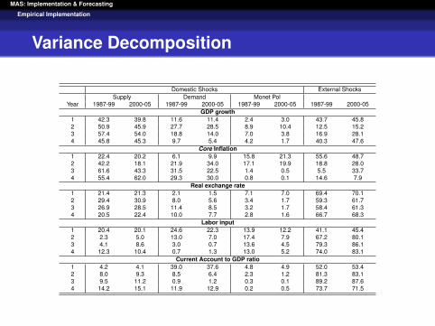
Variance Decomposition

Domestic Shocks External ShocksSupply Demand Monet Pol

Year 1987-99 2000-05 1987-99 2000-05 1987-99 2000-05 1987-99 2000-05GDP growth

1 42.3 39.8 11.6 11.4 2.4 3.0 43.7 45.82 50.9 45.9 27.7 28.5 8.9 10.4 12.5 15.23 57.4 54.0 18.8 14.0 7.0 3.8 16.9 28.14 45.8 45.3 9.7 5.4 4.2 1.7 40.3 47.6

Core Inflation1 22.4 20.2 6.1 9.9 15.8 21.3 55.6 48.72 42.2 18.1 21.9 34.0 17.1 19.9 18.8 28.03 61.6 43.3 31.5 22.5 1.4 0.5 5.5 33.74 55.4 62.0 29.3 30.0 0.8 0.1 14.6 7.9

Real exchange rate1 21.4 21.3 2.1 1.5 7.1 7.0 69.4 70.12 29.4 30.9 8.0 5.6 3.4 1.7 59.3 61.73 26.9 28.5 11.4 8.5 3.2 1.7 58.4 61.34 20.5 22.4 10.0 7.7 2.8 1.6 66.7 68.3

Labor input1 20.4 20.1 24.6 22.3 13.9 12.2 41.1 45.42 2.3 5.0 13.0 7.0 17.4 7.9 67.2 80.13 4.1 8.6 3.0 0.7 13.6 4.5 79.3 86.14 12.3 10.4 0.7 1.3 13.0 5.2 74.0 83.1

Current Account to GDP ratio1 4.2 4.1 39.0 37.6 4.8 4.9 52.0 53.42 8.0 9.3 8.5 6.4 2.3 1.2 81.3 83.13 9.5 11.2 0.9 1.2 0.3 0.1 89.2 87.64 14.2 15.1 11.9 12.9 0.2 0.5 73.7 71.5



Historical decomposition of GDP growth

1990 1995 2000 2005

−5

0

5

Quarters

devi

atio

n S

S (

%)

yt − yt−4/aH

1990 1995 2000 2005

−5

0

5

Quartersde

viat

ion

SS

(%

)

yt − yt−4/ζT

1990 1995 2000 2005

−5

0

5

Quarters

devi

atio

n S

S (

%)

yt − yt−4/yS

1990 1995 2000 2005

−5

0

5

Quarters

devi

atio

n S

S (

%)

yt − yt−4/ζL

1990 1995 2000 2005

−5

0

5

Quarters

devi

atio

n S

S (

%)

yt − yt−4/ζI

1990 1995 2000 2005

−5

0

5

Quarters

devi

atio

n S

S (

%)

yt − yt−4/ζC

1990 1995 2000 2005

−5

0

5

Quarters

devi

atio

n S

S (

%)

yt − yt−4/ζG

1990 1995 2000 2005

−5

0

5

Quarters

devi

atio

n S

S (

%)

yt − yt−4/ζm

1990 1995 2000 2005

−5

0

5

Quarters

devi

atio

n S

S (

%)

yt − yt−4/p∗

S

1990 1995 2000 2005

−5

0

5

Quarters

devi

atio

n S

S (

%)

yt − yt−4/p∗

O

1990 1995 2000 2005

−5

0

5

Quarters

devi

atio

n S

S (

%)

yt − yt−4/y∗

1990 1995 2000 2005

−5

0

5

Quarters

devi

atio

n S

S (

%)

yt − yt−4/i∗

1990 1995 2000 2005

−5

0

5

Quarters

devi

atio

n S

S (

%)

yt − yt−4/π∗

1990 1995 2000 2005

−5

0

5

Quarters

devi

atio

n S

S (

%)

yt − yt−4/ζ∗

F

1990 1995 2000 2005

−5

0

5

Quarters

devi

atio

n S

S (

%)

yt − yt−4

model

data



Historical Decomposition

Period Domestic Shocks External Shocks TotalSupply Demand Monet Pol

GDP growth90-93 1.55 0.25 -0.10 -0.37 1.3494-97 0.02 0.09 -0.39 2.08 1.8198-01 -3.29 -0.38 -0.10 0.20 -3.5602-05 -0.87 0.00 0.60 -0.27 -0.54

core inflation90-93 -1.25 0.09 -0.45 1.90 0.2994-97 -0.17 0.38 -1.27 0.39 -0.6798-01 1.79 0.36 -2.40 -0.18 -0.4202-05 -0.75 -0.18 0.43 -0.65 -1.15

Real exchange rate90-93 8.27 -0.43 -0.94 3.09 9.9994-97 4.76 -0.69 -2.22 -9.34 -7.4998-01 -2.76 -0.48 -5.28 0.06 -8.4602-05 -2.34 0.40 -1.05 9.26 6.26

Labor input90-93 2.31 0.05 -0.93 -6.75 -5.3294-97 0.87 0.24 -2.34 2.36 1.1298-01 1.60 0.27 -5.69 4.40 0.5902-05 -1.23 -0.39 -0.31 1.60 -0.33

Current Account to GDP ratio90-93 -3.50 -0.19 0.13 2.41 -1.1594-97 -0.52 -0.22 0.44 -0.87 -1.1898-01 2.43 -0.05 0.97 -3.60 -0.2502-05 2.40 0.32 -0.57 0.05 2.20


Forecasting

Forecasting with MAS

Fluctuations in observable variables is used to infer thesequences of shocks hitting the Chilean economy through thelens of the modelThis inference plus the estimated persistence of these shocksallow us to forecastWe add back constants removed from detrendingWe started in 2007 to carry out formal forecasts in parallel to thesemi-strcutural macro model as inputs for our Inflation ReportSome questions arisen:

How do the MAS forecasts compare to the one performed with thesemi-structural macro model?How is the quality of these forecasts?How to explain their results?


Forecasting

Forecasting: Comparable to the semi-structuralmacro model (core inflation)

05-II

0

1

2

3

4

5

2004 2005 2006 2007

MAS MEP Actual

05-III

0

0.5

1

1.5

2

2.5

3

3.5

4

4.5

5

2004 2005 2006 2007

06-I

0

1

2

3

4

5

2004 2005 2006 2007

06-II

0

1

2

3

4

5

2004 2005 2006 2007

06-III

0

1

2

3

4

5

2004 2005 2006 2007

06-III

0

1

2

3

4

5

2004 2005 2006 2007


Forecasting

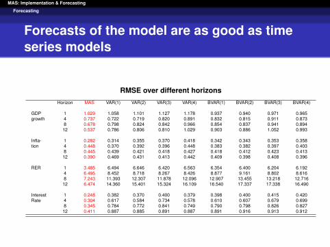
Forecasts of the model are as good as timeseries models

RMSE over different horizonsHorizon MAS VAR(1) VAR(2) VAR(3) VAR(4) BVAR(1) BVAR(2) BVAR(3) BVAR(4)

GDP 1 1.029 1.058 1.101 1.127 1.178 0.937 0.940 0.971 0.965growth 4 0.737 0.722 0.719 0.820 0.891 0.832 0.815 0.911 0.873

8 0.678 0.798 0.824 0.842 0.966 0.854 0.837 0.941 0.89412 0.537 0.786 0.806 0.810 1.029 0.903 0.886 1.052 0.993

Infla- 1 0.282 0.314 0.355 0.370 0.418 0.342 0.343 0.353 0.358tion 4 0.448 0.370 0.392 0.396 0.448 0.383 0.382 0.397 0.403

8 0.445 0.439 0.421 0.418 0.427 0.418 0.412 0.423 0.41312 0.390 0.469 0.431 0.413 0.442 0.409 0.398 0.408 0.396

RER 1 3.485 6.494 6.646 6.420 6.563 6.354 6.400 6.204 6.1924 6.495 8.452 8.718 8.267 8.426 8.877 9.161 8.802 8.6168 7.243 11.393 12.307 11.878 12.096 12.907 13.455 13.218 12.716

12 6.474 14.360 15.401 15.324 16.109 16.540 17.337 17.338 16.490

Interest 1 0.248 0.382 0.370 0.400 0.379 0.398 0.400 0.415 0.420Rate 4 0.304 0.617 0.584 0.734 0.578 0.610 0.607 0.679 0.699

8 0.345 0.784 0.772 0.841 0.749 0.790 0.798 0.826 0.82712 0.411 0.887 0.885 0.891 0.887 0.891 0.916 0.913 0.912


Forecasting

Explaining forecasts

The structure of the model allows us to perform a historicaldecomposition of forecastsHowever, the structure of model challenges the properidentification of shocks. Example: Food prices increase in 2007.

We adapt the model to include explicitly (exogenously) the behaviorof food prices in the model


Forecasting

Decomposition of forecast: Inflation

Decomposition: Core Inflation

Domestic Supply FactorsDomestic Supply FactorsDomestic Supply FactorsDomestic Supply Factors

-3.0-3.0-3.0-3.0

-2.0-2.0-2.0-2.0

-1.0-1.0-1.0-1.0

0.00.00.00.0

1.01.01.01.0

2.02.02.02.0

3.03.03.03.0

4.04.04.04.0

2000200020002000 2003200320032003 2006200620062006 2009200920092009

Domestic Demand FactorsDomestic Demand FactorsDomestic Demand FactorsDomestic Demand Factors

-3.0-3.0-3.0-3.0

-2.0-2.0-2.0-2.0

-1.0-1.0-1.0-1.0

0.00.00.00.0

1.01.01.01.0

2.02.02.02.0

3.03.03.03.0

4.04.04.04.0

2000200020002000 2003200320032003 2006200620062006 2009200920092009

MP shocksMP shocksMP shocksMP shocks

-3.0-3.0-3.0-3.0

-2.0-2.0-2.0-2.0

-1.0-1.0-1.0-1.0

0.00.00.00.0

1.01.01.01.0

2.02.02.02.0

3.03.03.03.0

4.04.04.04.0

2000200020002000 2003200320032003 2006200620062006 2009200920092009

External FactorsExternal FactorsExternal FactorsExternal Factors

-3.0-3.0-3.0-3.0

-2.0-2.0-2.0-2.0

-1.0-1.0-1.0-1.0

0.00.00.00.0

1.01.01.01.0

2.02.02.02.0

3.03.03.03.0

4.04.04.04.0

2000200020002000 2003200320032003 2006200620062006 2009200920092009

TotalTotalTotalTotal

-4.0-4.0-4.0-4.0

-3.0-3.0-3.0-3.0

-2.0-2.0-2.0-2.0

-1.0-1.0-1.0-1.0

0.00.00.00.0

1.01.01.01.0

2.02.02.02.0

3.03.03.03.0

4.04.04.04.0

2000200020002000 2003200320032003 2006200620062006 2009200920092009

Food PricesFood PricesFood PricesFood Prices

-3.0-3.0-3.0-3.0

-2.0-2.0-2.0-2.0

-1.0-1.0-1.0-1.0

0.00.00.00.0

1.01.01.01.0

2.02.02.02.0

3.03.03.03.0

4.04.04.04.0

2000200020002000 2003200320032003 2006200620062006 2009200920092009


Forecasting

Decomposition of forecast: Output

Decomposition: Output (w/o NNRR)

Domestic Supply FactorsDomestic Supply FactorsDomestic Supply FactorsDomestic Supply Factors

-3.0-3.0-3.0-3.0

-2.0-2.0-2.0-2.0

-1.0-1.0-1.0-1.0

0.00.00.00.0

1.01.01.01.0

2.02.02.02.0

3.03.03.03.0

4.04.04.04.0

2000200020002000 2003200320032003 2006200620062006 2009200920092009

Domestic Demand FactorsDomestic Demand FactorsDomestic Demand FactorsDomestic Demand Factors

-3.0-3.0-3.0-3.0

-2.0-2.0-2.0-2.0

-1.0-1.0-1.0-1.0

0.00.00.00.0

1.01.01.01.0

2.02.02.02.0

3.03.03.03.0

4.04.04.04.0

2000200020002000 2003200320032003 2006200620062006 2009200920092009

MP shocksMP shocksMP shocksMP shocks

-3.0-3.0-3.0-3.0

-2.0-2.0-2.0-2.0

-1.0-1.0-1.0-1.0

0.00.00.00.0

1.01.01.01.0

2.02.02.02.0

3.03.03.03.0

4.04.04.04.0

2000200020002000 2003200320032003 2006200620062006 2009200920092009

External FactorsExternal FactorsExternal FactorsExternal Factors

-4.0-4.0-4.0-4.0

-3.0-3.0-3.0-3.0

-2.0-2.0-2.0-2.0

-1.0-1.0-1.0-1.0

0.00.00.00.0

1.01.01.01.0

2.02.02.02.0

3.03.03.03.0

4.04.04.04.0

2000200020002000 2003200320032003 2006200620062006 2009200920092009

TotalTotalTotalTotal

-3.0-3.0-3.0-3.0

-2.0-2.0-2.0-2.0

-1.0-1.0-1.0-1.0

0.00.00.00.0

1.01.01.01.0

2.02.02.02.0

3.03.03.03.0

4.04.04.04.0

2000200020002000 2003200320032003 2006200620062006 2009200920092009

Food PricesFood PricesFood PricesFood Prices

-3.0-3.0-3.0-3.0

-2.0-2.0-2.0-2.0

-1.0-1.0-1.0-1.0

0.00.00.00.0

1.01.01.01.0

2.02.02.02.0

3.03.03.03.0

4.04.04.04.0

2000200020002000 2003200320032003 2006200620062006 2009200920092009


Forecasting

Further Issues on Forecasting with MAS

Some judgement introduced by adjusting constant terms indetrendingRisk analysis scenarios:

We use the IRFs to construct alternatives scenarios. Example:changes in terms of tradeWe modify the model to include elements that are part of the policydiscussions. Example: Transmission oil price shocks and lack ofMP credibility


Forecasting

Copper price shock

GDP (y/y %)

-0.6

-0.4

-0.2

0.0

0.2

0.4

0.6

0.8

Year 1 Year 2 Year 3 Year 4 Year 5

MAS MAS Alt. Fiscal Rule MEP

CPI Inflation (y/y %)

-0.1

0.0

0.1

0.2

0.3



Interes Rate

-0.1

0.0

0.1

0.3

0.4



Real Echange Rate

-0.6

-0.4

-0.2

0.0

0.2




Forecasting

Oil price shock

CPI Inflation (y/y %)

-0.3

0.0

0.3

0.6

0.9


MAS MEP

GDP (y/y %)

-0.2

-0.1

0.0

0.1

0.2


MAS MEP

Real Exchange Rate

-0.5

-0.2

0.0

0.2

0.5

0.7


MAS MEP

Interes Rate

-0.1

0.0

0.1

Year 1 Year 2 Year 3 Year 4 Year 5-0.40

-0.30

-0.20

-0.10

0.00

0.10

0.20

MAS MEP


Forecasting

Imperfect Credibility: Oil price shock

Headline Inflation Core Inflation Nominal Interest Rate

Output growth Real Exchange Rate Current Account (% of GDP)

Perfect Credibility Imperfect Credibility

-0.2

0.0

0.2

0.4

0.6

0.8

1.0

1.2

ye

ar

1 III

ye

ar

2 III

ye

ar

3 III

ye

ar

4 III

ye

ar

5 III

-0.1

0.0

0.1

0.2

0.3

0.4

0.5

0.6

0.7

0.8

0.9

ye

ar

1 III

ye

ar

2 III

ye

ar

3 III

ye

ar

4 III

ye

ar

5 III

-0.4

-0.3

-0.2

-0.1

0.0

0.1

0.2

ye

ar

1 III

ye

ar

2 III

ye

ar

3 III

ye

ar

4 III

ye

ar

5 III

-0.4

-0.2

0.0

0.2

0.4

0.6

0.8

ye

ar

1 III

ye

ar

2 III

ye

ar

3 III

ye

ar

4 III

ye

ar

5 III

-0.1

0.0

0.1

0.2

0.3

0.4

0.5

0.6

0.7

0.8

ye

ar

1 III

ye

ar

2 III

ye

ar

3 III

ye

ar

4 III

ye

ar

5 III

-0.4

-0.3

-0.2

-0.1

0.0

0.1

0.2

ye

ar

1 III

ye

ar

2 III

ye

ar

3 III

ye

ar

4 III

ye

ar

5 III


Conclusions and challenges

Conclusions and Challenges

MAS offers a coherent framework to perform policy analysisCommunication of MAS results: General equilibrium v/ssequential thinkingForecasts of MAS are comparable to the semi-structural modeland time series models. More on statistical inference of thequality of forecastsBenefits of the DSGE structure for the analysis of alternative/riskscenarios of the macroeconomic forecastSecular trends and relevant stationary ratiosObservable variables and historical decompositionChallenges with structure of model:

Role of relative price adjustments (particularly relevant for an openeconomy where exchange rate fluctuations play a central role)Labor market and exchange rate disconnectionMP rule and the implementation of the inflation forecast target inthe policy horizon

The MAS: a DSGE Model for Chile Implementation and Forecasting · The MAS: a DSGE Model for Chile...

Documents

Transcript of The MAS: a DSGE Model for Chile Implementation and Forecasting · The MAS: a DSGE Model for Chile...