The Marked Tree Site: Evaluation of Geosynthetic ...
219
2011 TRC0903 The Marked Tree Site: Evaluation of Geosynthetic Reinforcements in Flexible Pavements Brady R. Cox, Taylor M. Goldman, John S. McCartney Final Report
Transcript of The Marked Tree Site: Evaluation of Geosynthetic ...
2011
TRC0903
The Marked Tree Site: Evaluation of Geosynthetic
Reinforcements in Flexible Pavements
Brady R. Cox, Taylor M. Goldman, John S. McCartney
Final Report

THE MARKED TREE SITE: EVALUATION OF GEOSYNTHETIC REINFORCEMENTS IN FLEXIBLE PAVEMENTS
Final Report for project TRC 0903: Evaluation of Basal Reinforcement of Flexible Pavements with Geosynthetics
Submitted to the Arkansas State Highway and Transportation Department by:
Brady R. Cox, Ph.D., P.E. and
Taylor M. Goldman, The University of Arkansas
and John S. McCartney, Ph.D., P.E.,
The University of Colorado, Boulder
December 2011 University of Arkansas

ABSTRACT
This document presents findings from a three-year, full-scale, field research project
aimed at determining the benefits of using geosynthetic reinforcements to improve the
performance of flexible pavements constructed over poor subgrade soils. The test site, known as
the Marked Tree site, is an 850-ft (258-m) long segment of low-volume frontage road along
Highway 63 in the town of Marked Tree, Arkansas. The site, constructed in 2005, consists of
seventeen 50-ft (15.2-m) long flexible pavement test sections with various types of geosynthetic
reinforcements (woven and nonwoven geotextiles, and geogrids), which were all positioned at
the base-subgrade interface, and two different nominal base course thicknesses [6-in (15.2-cm)
and 10-in (25.4-cm)]. One section in each nominal base course sector was left unreinforced to
allow for monitoring of the relative performance between reinforced and unreinforced sections of
like basal thicknesses.
The different sections were evaluated in this study using deflection-based, surficial
testing conducted between 2008 and 2011, as well as subsurface forensic investigations
conducted in October 2010. Signs of serious pavement distress appeared in some of the test
sections in the Spring of 2010. Distress surveys revealed that all of the “failed” sections [defined
herein as sections with average rut depths > 0.5 in (1.3 cm)] had nominal base thicknesses of 6-in
(15.2-cm) and were reinforced with various geosynthetics. None of the sections with 10-in (25.4-
cm) nominal base thicknesses had “failed” despite receiving more than twice the number of
ESALs as the 6-in (15.2-cm) sections.
The impact of base course thickness was easily observed in the deflection-based test
results and rutting measurements. However, it was difficult to discern a consistent, clear trend of
better pavement performance relative to the various geosynthetic types in each nominal base

course thickness. Irrespective of geosynthetic reinforcement type (or lack thereof) all of the
sections that “failed” with respect to excessive rutting were the sections with the least combined
total pavement thickness (i.e., combined asphalt and base course thickness).

TABLE OF CONTENTS
LIST OF FIGURES
LIST OF TABLES
CHAPTER 1 - INTRODUCTION ................................................................................................1
1.1 Overview ................................................................................................................................1
1.2 Objectives ..............................................................................................................................3
1.3 Scope ......................................................................................................................................4
CHAPTER 2 - LITERATURE REVIEW ....................................................................................6
2.1 Overview ................................................................................................................................6
2.2 Introduction ............................................................................................................................6
2.3 Geosynthetic Materials ..........................................................................................................8
2.3.1 Geogrid ...........................................................................................................................8
2.3.2 Geotextile ........................................................................................................................9
2.4 Testing Methods.....................................................................................................................9
2.4.1 Laboratory Testing ........................................................................................................10
2.4.2 Full Scale Field Testing ................................................................................................14
2.4.3 Instrumented Test Sections ...........................................................................................15
2.5 Previous Research ................................................................................................................17
2.5.1 Evaluation of the Impact of Subgrade Strength ............................................................18
2.5.2 Evaluation of the Impact of Base Course Layer Thickness ..........................................22

2.5.3 Evaluation of Geosynthetic Location ............................................................................22
2.5.4 Evaluation of Geosynthetic Properties ..........................................................................23
2.6 Evaluation of Reinforcement Mechanisms ..........................................................................24
2.6.1 Lateral Restraint ............................................................................................................24
2.6.2 Separation .....................................................................................................................25
2.6.3 Tensioned-Membrane Effect ........................................................................................26
2.7 Design Methods ...................................................................................................................27
2.8 Conclusion from Literature Evaluation ...............................................................................28
CHAPTER 3 – SITE HISTORY ................................................................................................30
3.1 Overview ..............................................................................................................................30
3.2 Site Description ....................................................................................................................33
3.2.1 Site Location .................................................................................................................33
3.2.2 Site Characterization .....................................................................................................35
3.2.2.1 Sampling and Laboratory Testing .........................................................................35
3.3 Site Construction ..................................................................................................................40
3.3.1 Subgrade .......................................................................................................................40
3.3.2 Geosynthetics ................................................................................................................42
3.3.3 Base Course ..................................................................................................................48
3.3.4 Asphalt Layer ................................................................................................................51
3.4 Instrumented Testing Results (Summary) ...........................................................................53

CHAPTER 4 – PROJECT CONTINUATION .........................................................................56
4.1 Overview ..............................................................................................................................56
4.2 Introduction ..........................................................................................................................56
4.3 Initial Objectives of TRC 0903 ............................................................................................57
4.4 Testing History.....................................................................................................................59
4.5 Pavement Condition .............................................................................................................60
4.5.1 Traffic Loading .............................................................................................................61
4.5.2 Distress Survey .............................................................................................................64
4.6 Conclusions ..........................................................................................................................69
CHAPTER 5 – DEFLECTION-BASED TESTS TO INFER RELATIVE PERFORMANCE .............................................................................................71
5.1 Overview ..............................................................................................................................71
5.2 Falling Weight Deflectometer (FWD) .................................................................................72
5.2.1 FWD Testing Procedure ...............................................................................................73
5.2.2 FWD Data Analysis ......................................................................................................73
5.2.3 FWD Results .................................................................................................................76
5.3 Plate Load Test (PLT) ..........................................................................................................83
5.3.1 PLT Testing Procedure .................................................................................................84
5.3.2 PLT Data Analysis ........................................................................................................85
5.3.3 PLT Results ...................................................................................................................88
5.4 Accelerated Dynamic Deflectometer (ADD) .......................................................................90
5.4.1 ADD Testing Procedure ................................................................................................90
5.4.2 ADD Data Analysis ......................................................................................................93

5.3.3 ADD Results .................................................................................................................96
5.4.3.1 December 2009 ADD Results ................................................................................96
5.4.3.2 May 2011 ADD Results ..........................................................................................97
5.4.3.3 ADD Composite Ranking .......................................................................................97
5.5 Light Weight Deflectometer (LWD) .................................................................................104
5.5.1 LWD Testing Procedure .............................................................................................105
5.5.2 LWD Data Analysis ....................................................................................................106
5.5.3 LWD Results ...............................................................................................................108
5.6 Rolling Dynamic Deflectometer (RDD) ............................................................................112
5.6.1 RDD Testing Procedure ..............................................................................................113
5.6.2 RDD Data Analysis .....................................................................................................114
5.6.3 RDD Results ...............................................................................................................116
5.7 Composite Ranking from all Deflection-Based Test Results from the
Marked Tree Site ...............................................................................................................118
5.8 Composite Ranking from PLT and ADD Test Results from Marked Tree Site ................120
5.9 Conclusions from Deflection-Based Test Results .............................................................122
CHAPTER 6 – FORENSIC EXCAVATION AND SUBSURFACE LAYER PROPERTIES ..................................................................................................124
6.1 Overview ............................................................................................................................124
6.2 Introduction ........................................................................................................................124
6.3 Forensic Excavation ...........................................................................................................126
6.4 Layer Properties .................................................................................................................132
6.4.1 Layer Thicknesses .......................................................................................................132
6.4.2 Moisture Content ........................................................................................................136
6.4.3 Plasticity Index ............................................................................................................142
6.4.4 Dry Density .................................................................................................................144
6.5 Strength/Stiffness Testing ..................................................................................................149
6.5.1 Dynamic Cone Penetrometer (DCP) ...........................................................................149
6.5.1.1 DCP Testing Procedure........................................................................................150
6.5.1.2 DCP Data Analysis ..............................................................................................151
6.5.1.3 DCP Results .........................................................................................................154
6.5.2 In-Situ California Bearing Ratio (CBR) .....................................................................159
6.5.2.1 In-Situ CBR Testing Procedure ...........................................................................159
6.5.2.2 In-Situ CBR Data Analysis ..................................................................................161
6.5.2.3 In-Situ CBR Results .............................................................................................162
6.5.3 Resilient Modulus (MR) ..............................................................................................165
6.5.3.1 Resilient Modulus Testing Procedure ..................................................................166
6.5.3.2 Resilient Modulus Data Analysis .........................................................................170
6.5.3.3 Resilient Modulus Results ...................................................................................172
6.5.4 Unconsolidated Undrained (UU) Triaxial Test ...........................................................173
6.5.4.1 UU Testing Procedure ..........................................................................................175
6.5.4.2 UU Data Analysis ................................................................................................176
6.5.4.3 UU Results ...........................................................................................................178
6.6 Subsurface Layer Properties Composite Ranking .............................................................178
6.7 Conclusions Drawn from Subsurface Layer Properties .....................................................184

CHAPTER 7 – CONCLUSIONS AND RECOMMENDATIONS .........................................186
7.1 Summary ............................................................................................................................186
7.2 Conclusions ........................................................................................................................189
7.2.1 Rut Depth Measurements ............................................................................................189
7.2.2 Deflection-Based Tests to Infer Relative Performance ..............................................190
7.2.3 Subsurface Layer Properties .......................................................................................191
7.3 Recommendation for Future Work ....................................................................................193
CHAPTER 8 - REFERENCES .................................................................................................196

LIST OF FIGURES
Figure 2. 1. Cyclic Plate Load Test in laboratory tank ..................................................................12
Figure 2. 2. Heavy Vehicle Simulator (HVS) ................................................................................12
Figure 2. 3. Typical relationship between displacement and loading cycles. ................................12 Figure 2. 4. Permanent displacement profile at 800 cycles. ..........................................................12
Figure 2. 5. Average relative rut depth vs. cumulative ESALs .....................................................14
Figure 2. 6. Full-scale field testing ................................................................................................16
Figure 2. 7. Average rut depth after 75 and 150 truck passes ........................................................16
Figure 2. 8. Lateral base course restraint. ......................................................................................25 Figure 2. 9. Contribution of geotextile separation in pavements to prevent intermixing of layers ................................................................................................26 Figure 2. 10. Tensioned membrane effect .....................................................................................27
Figure 3. 1. Profile view of instrumentation configuration ...........................................................32
Figure 3. 2. Schematic of geosynthetic reinforced test sections in Marked Tree, Arkansas ..........................................................................................................32 Figure 3. 3. Arkansas state map featuring the project location ......................................................34
Figure 3. 4. Vicinity map of test site denoting approximate extent of test sections ......................34
Figure 3. 5. Test site prior to construction .....................................................................................35
Figure 3. 6. Subgrade soil profile based on Geotechnical exploration ..........................................37
Figure 3. 7. Plasticity index values of the subgrade from each section of the Marked Tree site from tests conducted in October 2004 .........................................39 Figure 3. 8. East facing view of geosynthetic overlap. ..................................................................41
Figure 3. 9. West facing view of geosynthetics in both lanes. .......................................................41
Figure 3. 10. Finished cut subgrade ...............................................................................................42

Figure 3. 11. Subgrade field nuclear density values from Marked Tree site construction .....................................................................................................43 Figure 3. 12. Geosynthetic tensioning technique. ..........................................................................46
Figure 3. 13. Geogrid strain gage protection, strip drain. ..............................................................48
Figure 3. 14. Geotextile strain gage protection, neoprene pad. .....................................................48
Figure 3. 15. Sand covering geosynthetic strain gage and cable. ..................................................48
Figure 3. 16. Crushed stone covering fine sand, geosynthetic strain gage, and cable. ...............................................................................................................49 Figure 3. 17. Base course placement on non-instrumented lane. ...................................................50
Figure 3. 18. Lateral placement of crushed limestone on geosynthetics. ......................................50
Figure 4. 1. Estimated ESALs per year. .........................................................................................63
Figure 4. 2. Average rut depths for measurements conducted in June of 2010. ............................66
Figure 4. 3. Average rut depths for measurements conducted in April of 2011. ...........................67
Figure 4. 4. Section 10 June 2010 distress survey. ........................................................................69
Figure 4. 5. Section 10 April 2011 distress survey. .......................................................................69
Figure 5. 1. Side and rear view of AHTD’s FWD at Marked Tree site .........................................74
Figure 5. 2. FWD testing locations at the Marked Tree site ..........................................................74
Figure 5. 3. Typical FWD deflections basins for Sections 1B and 13B from the May 2011 Marked Tree site visit .......................................................................75 Figure 5. 4. Total deflected area composite rankings from eight FWD tests conducted at the Marked Tree site ...........................................................................82 Figure 5. 5. AREA12 composite rankings from eight FWD tests conducted at the Marked Tree site ................................................................................................83 Figure 5. 6. University of Arkansas vibroseis truck ......................................................................85
Figure 5. 7. Rear and side view, respectively, of the PLT testing configuration at the Marked Tree site ............................................................................................86

Figure 5. 8. Typical PLT response curve for a 10-in (25.4-cm) base section (Section 6) .................................................................................................................87 Figure 5. 9. Typical PLT response curve for a 6-in (15.2-cm) base section (Section 13B) ...........................................................................................................87 Figure 5. 10. Average stiffness values calculated from PLT tests conducted at Marked Tree site in December, 2009 ......................................................................89 Figure 5. 11. ADD testing configuration using the University of Arkansas vibroseis truck ........................................................................................................92 Figure 5. 12. ADD testing configuration using the University of Texas vibroseis truck ........................................................................................................92 Figure 5. 13. Typical ADD deformation basin for a 10-in (25.4-cm) base section (Section 5) from testing in December 2009 ............................................................94 Figure 5. 14. Typical ADD deformation basin for a 6-in (15.2-cm) base section (Section 13B) from testing in December 2009 .......................................................94 Figure 5. 15. Total deformed area composite ranking from ADD testing at Marked Tree site ..................................................................................................103 Figure 5. 16. Deflected area up to 12” composite ranking from ADD testing at Marked Tree site ..................................................................................................103 Figure 5. 17. Δ12 composite ranking from ADD testing at Marked Tree site ..............................104
Figure 5. 18. Dynatest 3031 LWD schematic ..............................................................................107
Figure 5. 19. LWD tests conducted on asphalt and base course layers at Marked Tree site ..................................................................................................107 Figure 5. 20. Typical load-deflection pulses from LWD testing on the asphalt surface with 12-in (30.5-cm) loading plate at the Marked Tree site on 10-in (25.4-cm) and 6-in (15.2-cm) thick base course layers ..........................109 Figure 5. 21. Typical load-deflection pulses from LWD testing on the base layer with 12-in (30.5-cm) loading plate at the Marked Tree site on 10-in (25.4-cm) and 6-in (15.2-cm) thick base course layers .........................109 Figure 5. 22. ELWD results from LWD testing on the asphalt with 12-in (30.5-cm) diameter load plate ...............................................................................................110

Figure 5. 23. ELWD results from LWD testing on the base with a 12-in (30.5-cm) diameter loading plate ..........................................................................................111 Figure 5. 24. Schematic of RDD with important testing features labeled ...................................113
Figure 5. 25. University of Texas’s RDD at the Marked Tree site. .............................................115 Figure 5. 26. RDD Sensor 1 continuous deflection profile of the eastbound and westbound lanes at the Marked Tree site ...............................................................115 Figure 5. 27. Sensor 1 average deflections from RDD testing at the Marked Tree site ................................................................................................................117 Figure 5. 28. Composite ranking from all deflection-based testing at the Marked Tree site ..................................................................................................119 Figure 5. 29. Composite ranking from PLT and ADD testing at the Marked Tree site ................................................................................................................121 Figure 6. 1. Rut depth exceeding 3 inches (7.6 cm) in Section 13BW during May 2010 ...............................................................................................................125 Figure 6. 2. Excavation and testing area at Section 9 during October 2010 Marked Tree site visit ............................................................................................127 Figure 6. 3. Cutting (a) and removal (b) of asphalt layer for base course testing and sampling ..........................................................................................................128 Figure 6. 4. Nuclear density gauge readings conducted on the base (a) and subgrade (b) layers ..................................................................................................128 Figure 6. 5. DCP test conducted in southeast corner of excavation area of 13W ........................129
Figure 6. 6. CBR tests conducted on base (a) and subgrade (b) layers ........................................129
Figure 6. 7. Base layer excavation and sampling at Section 2 .....................................................130
Figure 6. 8. Base-subgrade interface of Section 1 (no geosynthetics) .........................................130
Figure 6. 9. Subgrade-geosynthetic interface of Section 1A (Mirafi geogrid) ............................131
Figure 6. 10. Shelby tube pushed in southwest corner of excavation area ..................................132
Figure 6. 11. Asphalt thicknesses collected during October 2010 site visit ................................134
Figure 6. 12. Base thicknesses collected during October 2010 site visit .....................................135

Figure 6. 13. Total asphalt and base section thicknesses collected during October 2010 site visit .........................................................................................135
Figure 6. 14. Desiccation crack in ground south of test site in October 2010 .............................138
Figure 6. 15. Pooling water on subgrade of Section 13W in October 2010 ................................138
Figure 6. 16. Standing water south of Sections 8 through 13B in May 2011 ..............................139 Figure 6. 17. Average in-situ base gravimetric moisture contents from samples collected in October 2010 .....................................................................................140 Figure 6. 18. Average in-situ gravimetric subgrade moisture contents from samples collected in October 2010 .......................................................................141 Figure 6. 19. Average plasticity index (PI) values of subgrade soils at Marked Tree test site ..........................................................................................................143
Figure 6. 20. Base in-situ dry densities calculated from October 2010 site visit ........................145 Figure 6. 21. Average subgrade in-situ dry densities determined from three testing procedures ................................................................................................148
Figure 6. 22. Schematic of Kessler K-100 DCP device ...............................................................151 Figure 6. 23. DCP testing at the Marked Tree site on December 2009 and October 2010, repsectively ..................................................................................152 Figure 6. 24. Typical DCP penetration curve for a 10-in (25.4-cm) nominal base thickness section (Section 3) from October 2010 site visit ..................................153 Figure 6. 25. Typical DCP penetration curve for a 6-in (15.2-cm) nominal base thickness section (Section 13BW) from October 2010 site visit .........................153 Figure 6. 26. Layer 1 (top of base) slopes calculated from DCP testing during the December 2009 Marked Tree site visit ...........................................................155 Figure 6. 27. Layer 2 (bottom of base) slopes calculated from DCP testing during the December 2009 Marked Tree site visit ..........................................................156 Figure 6. 28. Layer 3 (top of subgrade) slopes calculated from DCP testing during the December 2009 Marked Tree site visit ..........................................................156 Figure 6. 29. Layer 1 (top of base) slopes calculated from DCP testing during the October 2010 Marked Tree site visit...............................................................157 Figure 6. 30. Layer 2 (bottom of base) slopes calculated from DCP testing during the October 2010 Marked Tree site visit ..............................................................158

Figure 6. 31. Layer 3 (top of subgrade) slopes calculated from DCP testing during the October 2010 Marked Tree site visit ..............................................................158 Figure 6. 32. CBR testing setup and apparatus at Marked Tree site during October 2010 site visit .........................................................................................160 Figure 6. 33. Typical subgrade stress-penetration curve developed from data collected at Marked Tree site during October 2010 site visit ...............................162 Figure 6. 34. In-situ subgrade CBR values from the Marked Tree site during the October 2010 site visit ...................................................................................164 Figure 6. 35. Resilient modulus sample extrusion process: (a) Step 2, (b) Step 3, (c) Step 4 ..............................................................................................................167 Figure 6. 36. Resilient modulus specimen setup prior to placement of membrane and confining pressure cell ..................................................................................168 Figure 6. 37. Resilient modulus testing configuration for Marked Tree subgrade specimen ..............................................................................................................169 Figure 6. 38. Typical resilient modulus plot for Marked Tree subgrade specimen .....................172 Figure 6. 39. Subgrade resilient modulus results at 2 psi (13.8 kPa) confining pressure ................................................................................................................174 Figure 6. 40. Trautwein triaxial cell setup with subgrade sample for UU testing .......................177 Figure 6. 41. Normalized stress-strain curves of subgrade samples from Sections 6 and 10 ..................................................................................................179 Figure 6. 42. Subgrade undrained shear strength (Su) values calculated from UU testing ............................................................................................................180 Figure 6. 43. Subgrade layer properties composite rankings .......................................................182 Figure 6. 44. Base course layer properties composite rank .........................................................183

LIST OF TABLES
Table 2.1. Instrument survivability after 8 months ........................................................................18
Table 2.2. Summary of previous research test section properties ..................................................19
Table 2.3. Summary of previous research loading properties ......................................................19
Table 2.4. Summary of previous research geosynthetic properties and test results .....................20
Table 3.1. USCS soil classification of bulk samples from 2.5’ to 12.5’ .......................................38
Table 3.2. AASHTO soil classification ........................................................................................38
Table 3.3. Subgrade field nuclear density values .........................................................................43
Table 3.4. Crushed stone properties ..............................................................................................49
Table 3.5. As-built base course surveyed thicknesses ..................................................................52
Table 3.6. As-built asphalt core thicknesses .................................................................................54
Table 4.1. Summary of deflection and strength/stiffness tests conducted at Marked Tree site ..........................................................................................................61 Table 4.2. Truck factors for each vehicle classification ...............................................................64
Table 4.3. Average rut depths calculated from distress surveys ...................................................66
Table 5.1. FWD deflection basin area results from September 13, 2005 at the Marked Tree site ..........................................................................................................78 Table 5.2. FWD deflection basin area results from September 29, 2005 at the Marked Tree site ..........................................................................................................78 Table 5.3. FWD deflection basin area results from December 20, 2005 at the Marked Tree site ..........................................................................................................79 Table 5.4. FWD deflection basin area results from February 16, 2006 at the Marked Tree site ..........................................................................................................79 Table 5.5. FWD deflection basin area results from January 21, 2009 at the Marked Tree site ..........................................................................................................80 Table 5.6. FWD deflection basin area results from May 11, 2009 at the Marked Tree site ..........................................................................................................80

Table 5.7. FWD deflection basin area results from December 15, 2009 at the Marked Tree site ..........................................................................................................81 Table 5.8. FWD deflection basin area results from May 24, 2011 at the Marked Tree site ..........................................................................................................81 Table 5.9. Composite deflection basin area rankings from all eight FWD testing dates at the Marked Tree site ......................................................................................82 Table 5.10. Average stiffness values calculated from PLT tests conducted at Marked Tree site in December 2009 ...........................................................................89 Table 5.11. Static loading results from ADD testing on December 2009 at the Marked Tree site ........................................................................................................98 Table 5.12. ADD test results after 1,000 loading cycles on December 2009 at the Marked Tree site ..............................................................................................98 Table 5.13. ADD test results after 10,000 loading cycles on December 2009 at the Marked Tree site ..............................................................................................99 Table 5.14. ADD test results after 30,000 loading cycles on December 2009 at the Marked Tree site ..............................................................................................99 Table 5.15. Static loading results from ADD testing on May 2011 at the Marked Tree site ......................................................................................................101 Table 5.16. ADD test results after 1,000 loading cycles on may 2011 at the Marked Tree site ......................................................................................................101 Table 5.17. ADD test results after 2,500 loading cycles on May 2011 at the Marked Tree site ......................................................................................................102 Table 5.18. Composite rankings from ADD data analysis ..........................................................102 Table 5.19. ELWD results from LWD testing on the asphalt with 12-in (30.5-cm) diameter load plate ...................................................................................................110 Table 5.20. ELWD results from LWD testing on the base with a 12-in (30.5-cm) diameter loading plate ..............................................................................................111 Table 5.21. Average Sensor 1 deflections from RDD testing at the Marked Tree site .....................................................................................................................117 Table 5.22. Composite ranking from all deflection-based tests conducted at the Marked Tree site ................................................................................................119

Table 5.23. Composite ranking from PLT and ADD tests conducted at the Marked Tree site .......................................................................................................121 Table 6.1. Layer thicknesses collected during October 2010 site visit ........................................134 Table 6.2. Average in-situ gravimetric base moisture contents from the October 2010 site visit ..............................................................................................................139 Table 6.3. Average in-situ gravimetric subgrade moisture contents from the October 2010 site visit ................................................................................................140 Table 6.4. Average plasticity index (PI) values of subgrade soils at Marked Tree site ......................................................................................................................143 Table 6.5. Average in-situ dry density values of base and subgrade at the Marked Tree site obtained from nuclear gage total density and gravimetric water content ...............................................................................................................145 Table 6.6. Subgrade dry densities from resilient modulus test samples ......................................147 Table 6.7. Subgrade dry densities from UU triaxial test samples ................................................147 Table 6.8. Average subgrade dry densities from three determination procedures .......................148 Table 6.9. DCP results from the December 2009 Marked Tree site visit ....................................155 Table 6.10. DCP results from the October 2010 Marked Tree site visit .....................................157 Table 6.11. Subgrade in-situ CBR values from the Marked Tree site during October 2010 testing .................................................................................................164 Table 6.12. Subgrade resilient modulus results at 2 psi (13.8 kPa) confining pressure ....................................................................................................................174 Table 6.13. Subgrade undrained shear strength (Su) values calculated from UU testing .................................................................................................................179 Table 6.14. Subgrade layer properties composite rank ................................................................182 Table 6.15. Base course layer properties composite rank ............................................................183

1
Chapter 1
1.0 Introduction
1.1 Overview
In late 2004, the Arkansas Highway and Transportation Department (AHTD) began
construction of a low-volume frontage road (Frontage Road 3) along US Highway 63 in the town
of Marked Tree, Arkansas at the intersection of Arkansas Highway 75. An 850-ft (258-m) long
segment of this frontage road was utilized for a research project (AHTD TRC-0406) aimed at
determining the benefits, if any, of using geosynthetics to improve the performance of flexible
pavements on state funded roadway projects where poor subgrade soils were encountered. This
full-scale field study consisted of seventeen different 50-ft (15.2-m) long flexible pavement
sections constructed over poor subgrade soils (CH or A-7-6). Eight of these sections were
constructed with a 10-in (25.4-cm) nominal base course thickness and eight were constructed
with a 6-in (15.2-cm) nominal base thickness. The section in the middle served as a transition
between the two sectors with different nominal base course thicknesses. Seven of the eight
sections in each nominal base course sector were reinforced with various geosynthetics (woven
and nonwoven geotextiles, and geogrids), which were all positioned at the base-subgrade
interface of the roadway. One section in each nominal base course sector was left unreinforced to
allow for monitoring of the relative performance between reinforced and unreinforced sections of
like basal thicknesses.
The sixteen test sections were instrumented with earth pressure cells and strain gauges
applied to the geosynthetics and the asphalt. The transition section was instrumented with earth
pressure cells, control strain gauges (geosynthetics and asphalt) for environmental calibration,

2
moisture content probes, thermocouples, and piezometers. However, this instrumentation was
only monitored for a limited period of time (approximately 6 months) between September 2005
and March 2006 under normal and accelerated traffic loading. Limited conclusions were drawn
from this monitoring (Howard 2006, Warren and Howard 2007a & 2007b) and the project was
abandoned until July 2008. At this time, the Marked Tree project was re-started as research
project AHTD TRC-0903, with the goal of continuing to monitor the instrumented sections.
Unfortunately, all of the instrumentation, with exception of the asphalt strain gauges, had failed
during the two-plus year gap in monitoring. Detailed information on the history of the Marked
Tree site is found in Chapter 3.
Since the original instrumentation was no longer functioning, the new research group
decided to monitor the relative performance of the test sections through a combination of
surficial and subsurface testing. The surficial testing techniques consisted primarily of
deflection-based tests such as the Falling Weight Deflectometer (FWD), static Plate Load Test
(PLT), Accelerated Dynamic Deflectometer (ADD), and Light Weight Deflectometer (LWD).
Results from these tests were used to infer relative pavement performance between test sections.
These tests and results are described in great detail in Chapter 5.
Signs of serious pavement distress (primarily deep rutting with some alligator cracking)
appeared in some of the test sections in the spring of 2010, leading AHTD to document the
pavement performance with manual distress surveys in June of 2010 and April of 2011. These
distress surveys revealed that a few sections of the roadway, especially in the westbound lane,
were performing poorly. All of the “failed” sections [defined herein as sections with average rut
depths > 0.5 in (1.3 cm)] were located in the sector with 6-in (15.2-cm) nominal base thickness.
Furthermore, traffic surveys conducted during this time frame indicated that the 10-in (25.4-cm)

3
nominal base course sections had received more than twice the number of ESALs over the life of
the pavement than the 6-in (15.2-cm) nominal base course sections. Detailed information about
the traffic and distress surveys conducted at the Marked Tree site is provided in Chapter 4.
The research team was tasked with trying to figure out why certain 6-in (15.2-cm)
nominal base course sections had “failed”, while others had not. A subsurface forensic
investigation was completed on each test section during a site visit in October 2010. The
subsurface investigation was conducted so the research group could gather information
concerning subsurface layer properties (i.e., in-situ dry density, in-situ moisture content,
plasticity index, etc.), as well as subsurface relative strength/stiffness values (in-situ CBR, DCP
penetration resistance, laboratory resilient modulus and undrained shear strength), to determine
what properties, or combinations of properties, were causing some sections to fail while the rest
of the sections performed substantially better. Results from the subsurface forensic excavation
are presented in Chapter 6.
1.2 Objectives
The main objective of this work was to quantify the performance benefits, if any, from
using geosynthetic reinforcements in flexible pavements on state funded roadway projects where
soft subgrade soils were encountered. The findings presented herein were derived from an
extensive investigation of a full-scale reinforced pavement with a current life of over 6 years.
Absolute and relative pavement performance has been quantified through cracking and rut depth
data collected during distress surveys conducted in June 2010 and April 2011. Surficial
deflection-based tests conducted between September 2005 and May 2011 have been analyzed to
determine which test(s) and data analysis method(s) can best be used to best infer the observed
pavement performance. Additionally, subsurface investigations within the pavement test sections

4
have been conducted to determine if differences in the base and subgrade properties across the
site significantly influenced the observed pavement performance.
A ranking system (from 1 through 16) has been used throughout this work to distinguish
the “best” sections from the “worst” sections based on every test conducted at the site. The
surficial deflection-based tests and subsurface layer properties have been synthesized in terms of
these rankings to arrive at a final evaluation of the sections relative to the observed pavement
rutting measurements. While the data is not perfect, and at times perplexing for any individual
test, the one thing that seems to stand out is that irrespective of geosynthetic reinforcement type
(or lack thereof) all of the sections that have “failed” via rutting are also the sections with the
least combined total pavement thickness (i.e., asphalt plus base thickness). Therefore, a clear
benefit from utilizing geosynthetic reinforcements at the Marked Tree site was not observed
either through the deflection-based testing program or through the observed pavement rutting.
1.3 Scope
The following is an outline of the subsequent chapters, as well as a brief description of
each chapter:
Chapter 2 outlines the literature review on geosynthetic reinforcements installed in flexible pavement structures.
Chapter 3 presents site information (i.e., geographic location and site construction), as well as results from soil testing prior to construction.
Chapter 4 contains information about the testing history of research projects TRC-0406 and TRC-0903, project objectives, estimated traffic loading derived from traffic count data collected from January to August of 2011, and the pavement condition as of April 2011.
Chapter 5 presents the methods of conducting and analyzing the surficial deflection-based tests conducted throughout the life of the roadway.

5
Chapter 6 presents information gathered during the subsurface forensic investigation in October 2010, as well as testing methods and results from samples collected during the subsurface investigation.
Chapter 7 contains conclusions drawn from the data presented in the previous chapters and recommendations for future studies on the Marked Tree site and other similar geosynthetic reinforced pavements.

6
Chapter 2
2.0 Literature Review
2.1 Overview
The focus of this chapter is to discuss and summarize information collected through
researching technical literature associated with flexible pavement structures reinforced with
geosynthetic materials. More specifically, this review will closely examine studies involving the
construction and testing of pavement structures with and without geosynthetic reinforcements.
There have been many projects geared toward quantifying the beneficial effects of geosynthetic
reinforcements installed in flexible pavement structures. However, many of these projects have
differed in both their approach (in-situ vs. laboratory testing) and materials used (various types
of soils, geosynthetics, configurations, etc.). The goal of this review is to analyze the findings
from the researched literature to develop a sense of how and under what circumstances
geosynthetic reinforcement benefit flexible pavement structures. The types of tests previously
used to analyze the benefits from geosynthetic reinforcements in pavement structures will be
investigated to conclude which of the testing methods most accurately detects and describes the
reinforcement potential. However, discrepancies from one study to the next, as well as the lack
of a universally accepted design standard, provide uncertainties in design and application.
2.2 Introduction
Flexible pavements usually consist of a bituminous surface underlain with a layer of
granular material and a layer of a suitable mixture of coarse and fine materials. These structures
are designed so that traffic loads are transferred by the wearing surface (asphalt layer) to the
underlying supporting materials through the interlocking of aggregates, the frictional effect of

7
the granular materials, and the cohesion of the fine materials (Garber and Hoel 2002). With the
assumptions of these materials transferring the loads as anticipated, the pavement structure is
expected to support a designed amount of traffic over the desired life of the structure. Most
premature pavement failures are structural in nature, meaning that one or more of the materials in
the system have reached a mechanical failure state. Structural failures in pavement structures
occur due to unexpected variables or variations in design factors that change the pavement
materials such as: unexpected loadings, environmental interaction, drainage problems, and other
factors such as cyclic degradation, frost heave, and subgrade settlement. In order to counter some
of these adverse effects, engineers, owners, and contractors commonly incorporate practices such
as thick structural pavement sections to account for weak subgrade soil conditions (Archer
2008). However, the practice of constructing thicker base layers to accommodate for poor
subgrade soils can accrue excessive costs in many situations.
The implementation of geosynthetic reinforcements in the pavement structure can be an
advantageous alternative by increasing the pavement service life and reducing the cost in lieu of
more expensive natural materials (Brandon et al. 1996). Geosynthetic materials have been
proven to be effective as reinforcement materials in slope stability applications and retaining
walls, and for over 30 years, geosynthetics have been applied to experimental pavement
structures due to the expected potential to improve pavement performance. In slopes and
retaining walls, the soil transfers shear stresses to the geosynthetic reinforcements, which resist
these imposed stresses through mobilized tensile resistance. Numerous field and lab studies have
illustrated that geosynthetic reinforcements applied in the base course of pavement structures
have the capability to improve bearing capacity, extend the service life, reduce the necessary fill
thickness, reduce differential settlement, and delay rut formation (Hufenus et al. 2005).

8
2.3 Geosynthetic Materials
Geosynthetic materials are fabric-like materials made from polymers such as polyvinyl
chloride (PVC), polyethylene, polypropylene, and polyester (Das 2006). The term geosynthetics
represents many types of construction materials that serve several purposes, but the two forms of
geosynthetics that are most widely used in pavement systems are geogrids and geotextiles (Al-
Qadi et al. 1994). Although both of these reinforcements may contribute to pavement
performance, Al-Qadi et al. (1994) found that the mechanisms by which the two types reinforced
the pavement are different.
2.3.1 Geogrid
A geogrid is a geosynthetic material constructed of longitudinal and transverse ribs that
create openings referred to as apertures. These apertures are of sufficient size to allow strike-
through of surrounding soil, stone, or other geotechnical material (Koerner 2000). The
interlocking potential of geogrids allows them to be ideal reinforcement in granular layers, such
as the base course of a pavement structure. When the surface of a pavement structure reinforced
with a geogrid is vertically loaded, the granular materials will become interlocked with the
geogrid. The interlocking effect restrains the aggregate laterally and transmits tensile forces from
the aggregate to the geogrid (Maubeuge 2011). By laterally restraining the soil, the geogrid
contributes in preventing lateral spreading of the base aggregate, increasing the strength of the
base in the vicinity of the reinforcement, improving vertical stress distribution on the subgrade,
and reducing shear stress in the subgrade (Berg et al. 2000). In this mechanism, the geogrid does
not likely go into tension unless higher strains are observed in the system (Giroud and Noiray
1981).

9
2.3.2 Geotextile
The geotextiles typically used for reinforcement applications are woven filament sheets
(Koerner 2000), however, nonwoven geotextiles have also been used. The main reinforcement
mechanism provided by woven geotextiles is separation. A geosynthetic placed at the interface
between the aggregate base course and the subgrade functions as a separator to prevent two
dissimilar materials (subgrade soils and aggregates) from intermixing (Berg et al. 2000).
Separation allows a stiff material placed on a soft subgrade to maintain its full thickness
throughout the life of the pavement. In order to mobilize tensile resistance, it is possible that the
geosynthetics have to be subjected to strains close to those prompted by failure induced loading,
similar to geogrid tensile mobilization. Cuelho and Perkins (2009) suggested that the puncture
resistance of the geotextile should be taken into account, as penetration of particles through the
geotextile will reduce its strength and stiffness (Cuelho and Perkins 2009).
2.4 Testing Methods
Geosynthetic-reinforced pavement test sections have been constructed and evaluated over
the past 30 years and, as a whole, have demonstrated positive and significant benefits provided
by reinforcement (Perkins and Cortez 2005). Though the general consensus from past research
efforts describe that pavement structures have been improved through the installation of
geosynthetic reinforcements, there are too many discrepancies between test methods attempting
to quantify the performance benefits of incorporating geosynthetic reinforcements in flexible
pavement structures. There are basically three methods for testing the contributions of
geosynthetic reinforcements in pavement structures as follows: (1) cyclic loading of laboratory
contained test sections (box tests), (2) controlled-traffic track tests that apply loads with standard
trucks and moving wheel loads (MWL) single wheel load applicators, and (3) full-scale field test
10
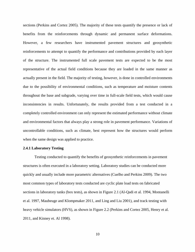
sections (Perkins and Cortez 2005). The majority of these tests quantify the presence or lack of
benefits from the reinforcements through dynamic and permanent surface deformations.
However, a few researchers have instrumented pavement structures and geosynthetic
reinforcements to attempt to quantify the performance and contributions provided by each layer
of the structure. The instrumented full scale pavement tests are expected to be the most
representative of the actual field conditions because they are loaded in the same manner as
actually present in the field. The majority of testing, however, is done in controlled environments
due to the possibility of environmental conditions, such as temperature and moisture contents
throughout the base and subgrade, varying over time in full-scale field tests, which would cause
inconsistencies in results. Unfortunately, the results provided from a test conducted in a
completely controlled environment can only represent the estimated performance without climate
and environmental factors that always play a strong role in pavement performance. Variations of
uncontrollable conditions, such as climate, best represent how the structures would perform
when the same design was applied to practice.
2.4.1 Laboratory Testing
Testing conducted to quantify the benefits of geosynthetic reinforcements in pavement
structures is often executed in a laboratory setting. Laboratory studies can be conducted more
quickly and usually include more parametric alternatives (Cuelho and Perkins 2009). The two
most common types of laboratory tests conducted are cyclic plate load tests on fabricated
sections in laboratory tanks (box tests), as shown in Figure 2.1 (Al-Qadi et al. 1994, Montanelli
et al. 1997, Maubeuge and Klompmaker 2011, and Ling and Liu 2001), and track testing with
heavy vehicle simulators (HVS), as shown in Figure 2.2 (Perkins and Cortez 2005, Henry et al.
2011, and Kinney et. Al 1998).

11
Cyclic plate load testing in laboratory tanks (box tests) cannot be considered exactly
representative of full-scale pavements due to boundary and scaling effects. Specifically, the size
of the test section and layer thicknesses are reduced; however, the distribution of soil particle
sizes (gradation curve) or geosynthetic properties are not scaled down in the same manner as the
section sizes. When analyzing results from ‘box tests’ it must be considered that there is only a
small section of pavement structure being tested that is enclosed by much superior materials,
often concrete walls. The test results may be influenced by stress waves passing through the soils
and rebounding off of the boundaries and back into the structure. The constraints of the
boundaries help prevent lateral displacement which would simulate a response from the structure
different than that if the section being tested was surrounded by a much larger area of like
materials.
Montanelli et al. (1997) performed cyclic plate load tests on sections reinforced with
geogrid. This test was performed by applying 300,000 sinusoidal loading cycles through a 12-in
(300-mm) diameter circular loading plate providing 0 to 9 kips (0 - 40 kN) [maximum applied
pressure of 82 psi (570 kPa)] at frequencies of 5 and 10 Hz (Montanelli et al. 1997). Al-Qadi et
al. (1994) performed a similar test, except the loading frequency was 0.5 Hz, and presented a
goal of testing until at least one inch (25 mm) of displacement had occurred (Al-Qadi et al.
1994). Al-Qadi et al. (1994) also tested geotextiles as well as a geogrid in comparison to a
control section. The typical presentation of data collected from these tests is a comparison of
surface deformation at a given location versus number of loading cycles of the applied load, as
well as a cross-sectional profile of surface deformation at a specified number of loading cycles.
Figures 2.3 and 2.4 are examples of the latter mentioned data presentation methods, respectively,
via Al-Qadi et al. (1994). As observed in Figure 2.4, the control was the poorest performing

F la
Figure displac (Al-Qa
igure 2.1. Cyaboratory tan
e 2.3. Typicacement and ladi et al. 199
yclic Plate Lnk (Al-Qadi
al relationshiloading cycl94).
Load Test in et al. 1994).
ip betweenles
12
Figure. (Perki
Figu at 80
e 2.2. Heavy ins and Cort
ure 2.4. Perm00 cycles (A
Vehicle Simez 2005).
manent displAl-Qadi et al
mulator (HV
acement pro. 1994).
S)
ofile

13
section after 800 loading cycles were applied, but the geotextiles unexpectedly outperformed the
geogrid.
Other studies involve laboratory testing using heavy vehicle simulators (HVS) (Perkins
and Cortez 2005, Henry et al. 2011, and Kinney et al. 1998). The use of HVS systems are more
representative of actual pavement loading because larger test sections are constructed and rolling
wheel loads are used; however, the construction and testing of these test sections are often time
consuming and expensive. This is especially the case if site-specific soils need to be transported
to the HVS location. The testing facilities are normally constructed indoors in long rectangular
pits (Perkins and Cortez 2005 and Henry et al. 2011) or outdoor test tracks constructed of more
representative boundaries, such as plywood surrounded by gravel and sand rather than concrete
walls (Kinney et al. 1998). The sections are loaded using a load frame with a wheel attached that
travels unidirectionally along the longitudinal axes of the text sections (Perkins and Cortez
2005). The test sections are typically loaded to a finite number of Equivalent Single Axle Loads
(ESALs), which are equivalent to 18 kip (80 kN), or until failure (Henry et al. 2011). Henry et al.
(2011) presented testing results as average rut depth versus cumulative ESALs for all sections
tested. This data presentation is displayed as Figure 2.5.
It can be observed in Figure 2.5 that the section with 6 inches (150 mm) of asphalt and 12
inches (300 mm) of base performed contradictory of what would be expected. The unreinforced
section resulted with less rut depth than the geosynthetic reinforced section after equivalent
ESALs were applied. However, it must be noted that the base course in the unreinforced section
was significantly softer, with a base modulus from FWD back calculations of approximately 30.6
ksi (281 MPa) (Henry et al. 2011). It should also be noticed that the thickest overall section,
asphalt and base layers combined, resulted in negligible differences in rutting between the

Figure 2.
reinforce
regard to
of base c
the pavem
2.4.2 Ful
F
environm
However
cannot be
variation
geosynth
times a g
section d
to preven
.5. Average r
ed and unrei
o grid reinfor
course is app
ment structu
ll Scale Fiel
ull scale tes
mental, and b
r, this can b
e controlled.
ns in the sub
hetic materia
geosynthetic
during testin
nt traffickin
relative rut d
inforced sec
rcement (He
plied, the mo
ure has reach
d Testing
sting is typic
boundary co
be inconveni
. Field test si
bgrade profil
al in the pave
c liner is us
g. Construct
ng of the sec
depth vs. cum
tions. This c
enry et al. 20
obilization o
hed the point
cally perform
onditions en
ient and unc
ites also prev
le. Therefor
ement design
ed to elimin
tion quality
ctions prior
14
mulative ESA
could repres
011). It coul
of the geosyn
of failure.
med to eval
ncountered in
certain as th
vent control
re, to be abl
n, a uniform
nate migrati
control and
to traffic lo
ALs (Henry
sent a point
ld be possibl
nthetic reinfo
luate pavem
n a given ar
he environme
l of uniform
le to underst
m testing mat
on of the n
assurance m
oads being a
y et al. 2011)
of diminish
le that once
forcement is
ments under t
rea, as show
ental and lo
site conditio
tand that co
terial must b
natural subgr
must be mon
applied. Per
).
hing returns
a certain am
not reached
the actual tr
wn in Figure
oading condi
ons due to na
ontribution o
be used and
rade into the
nitored strict
rformance o
with
mount
d until
raffic,
e 2.6.
itions
atural
of the
often
e test
tly as
f test

15
sections is usually quantified by comparing average rut depths or surface deflections versus type
of section, such as Figure 2.7, (White et al. 2011, Cuelho et al. 2011, Tingle and Jersey 2009, and
Hufenus et al. 2006). Other testing methods of full scale test sections have been performed to
observe the quality of the structure after being trafficked. Joshi and Zornberg (2011) used falling
weight deflectometer (FWD) data to quantify the relative performance of reinforced pavement
sections . FWD tests were performed periodically throughout the life of the tested structure to
analyze the deflection basins created by the FWD in each section to identify layer properties and
to quantify relative damage to the pavement layers. Distress survey results were also compared
to the deflection data (Joshi and Zornberg 2011). Cox et al. (2010a) presents a test method that
uses a Vibroseis (shaker) truck to perform cyclic plate load (CPL) tests on geosynthetic
reinforced flexible pavements. The results from the latter test presented definite improvements in
pavement performance with increasing basal thickness, but the effects of the geosynthetic
reinforcements were not clearly defined, possibly because more surface deflection was needed to
mobilize the potential contributions from the geosynthetics (Cox et al. 2010a).
2.4.3 Instrumented Test Sections
Normally, both laboratory and full scale field tests only measure surface behavior of
tested sections. However, many times the problematic area is not the surface, or cannot be
observed from the surface. When moisture builds up in the pavement base and subgrade layer,
the shear strength in these layers begins to decrease and weaken. The weakening of the subgrade
soils can cause fatigue cracking and rutting in the pavement, but it is a result of wet conditions,
causing the subgrade and base course to mix, the drainability of the materials to decrease, and a
reduction in the initial design thickness of the pavement (Warren and Howard 2007a). While
there is evidence from field experiments, laboratory investigations and numerical evaluations

Figure 2.(Cuelho a
that supp
Howard 2
benefit th
within th
loading.
(1996), W
Issues in
lack of
instrumen
obtain va
table of i
fairly dec
instrumen
.6. Full-scaleand Perkins
ports the ben
2007a), ther
he structure
he test sectio
Several stud
Warren and
collecting v
informatio
ntation in g
aluable infor
instrument s
cent survivab
ntation. The
e field testin2009).
nefits of geos
re is a lack of
and affect th
on is needed
dies have be
Howard (20
valuable resu
on on prop
geosynthetic
rmation (Bra
urvivability
bility for the
e survivabilit
g
synthetic inc
f knowledge
he other laye
d to determin
een done on
007b) and W
ults from pre
per instrum
reinforced
andon et al.
after 8 mon
e majority of
ty could dras
16
Figure 2. truck pas
clusions in a
e and confide
ers. Therefo
ne what is h
n instrument
Warren et al
eviously ins
ment select
roadways hi
1996 and W
nths (Brando
f the instrum
stically go d
7. Average rsses (White e
flexible pav
ence as to ho
ore, a testing
happening a
ted test sect
l. (2008), bu
trumented p
tion and i
istorically d
Warren and H
on et al. 1996
ments, the rat
down over tim
rut depth aftet al. 2011).
vement struc
ow the geosy
g method tha
as a function
tions, such a
ut results ha
pavements ar
installation.
does not last
Howard 2007
6). Though t
tes are only
me, but Bran
ter 75 and 15
cture (Warren
ynthetics act
at measures s
n of depth d
as Brandon
ave been lim
re associated
Therefore,
t long enoug
7b). Table 2.
the table dis
after 8 mont
ndon et al. (1
50
n and
tually
strain
during
et al.
mited.
d to a
, the
gh to
1 is a
splays
ths of
1996)

17
only presents the data from one date. It is likely that the non-survived instruments were damaged
at installation and would have survived if a proper installation process was available. Weak spots
are also created in the pavement layers due to poor compaction around the instrumentation.
2.5 Previous Research
Numerous studies have been conducted to determine the performance of geogrid- and
geotextile-reinforced flexible pavement structures. The research presented in Tables 2.2, 2.3, and
2.4 (Berg et al. 2000 and Cox et al. 2010b) are laboratory and full scale field tests that quantify
the contribution of the geosynthetic reinforcements in pavement performance by examining
surface deflections. Table 2.2 is a summarization of the properties of several tests conducted on
the topic of geosynthetic reinforcements in flexible pavement structures. This includes soil
classifications, test type, testing area dimensions, and layer thicknesses. Table 2.3 summarizes
the loading properties of each test, such as loading type, applied load and frequency of loading.
Table 2.4 is the summarization of the geosynthetic reinforcements’ properties and the location in
the pavement structure for each testing instance. Table 2.4 also contains information on the
subbase thickness, the California Bearing Ratio (CBR) of the subgrade, surface deformations,
and the benefit of the geosynthetic reinforcement in terms of the traffic benefit ratio (TBR). The
TBR is the ratio of the number of loading cycles on the geosynthetic reinforced test section to
reach a certain rut depth to the number of loading cycles it takes a non-reinforced test section to
reach the same rut depth (Tencate 2010). All the studies examined in this section were conducted
on paved roadways, and they all provide some insight into potential benefits of geosynthetics as
reinforcement in flexible pavement structures (Berg et al. 2000). These studies also help
summarize how many different variables can impact reinforced pavement structure performance.
Each of these variables are very difficult to assess individually because they are interrelated, but

18
Table 2.1. Instrument survivability after 8 months (Brandon et al. 1996).
many have similar behaviors over a large range of different configurations. Trends found in these
variables developed from previous tests have been summarized in Tables 2.2, 2.3, and 2.4 (Cox
et al. 2010b).
2.5.1 Evaluation of the Impact of Subgrade Strength
The relevance of the different reinforcement mechanisms may depend on the subgrade
soil atop which the pavement rests. With a high quality subgrade beneath the pavement structure,
the reinforcement may never reach the stain level needed to be mobilized. Softer subgrade soils
will allow for much greater deformations, which will then begin to reach the strain levels
required to mobilize the geosynthetic reinforcement. California Bearing Ratio (CBR) is a
measure of the mechanical strength of a subgrade and is a design criterion for pavement
structures when choosing a suitable subgrade soil. The greater the CBR value, the stiffer the
subgrade is. Subgrades with CBR values less than 8 see the most benefit from geosynthetic
reinforcement (Tencate 2010). The reinforcement can be viewed as improving the bearing
capacity of the subgrade as it aids in supporting construction traffic, and the reinforcement can
help prevent differential settlements by bridging over weaker areas and transferring load to the
stronger areas if subgrade turns out to be heterogeneous (Perkins et al. 2005).
Kulite earth pressure cells 6 3 50%Carlson earth pressure cells 21 16 76%HMA strain gages 35 26 74%Geotextile strain gages 18 1 6%Geogrid strain gages 18 5 28%Soil strain gages 6 5 83%Thermocouples 17 15 88%Gypsum blocks 18 18 100%
Gage TypeNumber Installed
Number Survived
Percent Survived

Table 2.2
Table 2.3
2. Summary
3. Summary
of previous
of previous
research tes
research loa
19
st section pro
ading proper
operties (Cox
rties (Cox et
x et al. 2010
al. 2010b).
0b).

Table 2.4(Cox et a
4. Summary al. 2010b).
of previous research geo
20
osynthetic pr
roperties andd test resultss

Table 2.4(Cox et a
4 (continuedal. 2010b).
d). Summary of previous
21
research ge
osynthetic pproperties annd test resultss

22
2.5.2 Evaluation of the Impact of Base Course Layer Thickness
Geosynthetic reinforcements have been shown to increase structural performance of
pavements; therefore, geosynthetic reinforcements are sometimes used to reduce the thickness of
the base course while maintaining an equivalent service life (Perkins et al. 2005). Pavements
reinforced with geosynthetics on weaker subgrades, CBR=1, cannot reduce the base course layer
and maintain the same structural integrity (Haas et al. 1988). However, on subgrades with
adequate strength, CBR=8, the base course layer can be reduced by as much as 50% (Webster
1993). There is no definitive relationship between geosynthetic reinforcement and equivalent
base course thickness that can be replaced.
2.5.3 Evaluation of Geosynthetic Location
The ideal location of the geosynthetic reinforcement within the pavement layer is
dependent on the magnitude of the applied load and the quality and thickness of the pavement
structure being reinforced (Berg et al. 2000, Barksdale et al. 1989, and Haas et al. 1988). Even
though there are many parameters, such as subgrade quality, layer thicknesses, geosynthetic type,
and predicted loading, that can affect the “correct” placement of the geosynthetic reinforcement
in the flexible pavement structure; the most effective placement of the geotextile is always at a
layer interface, acting as a separator to keep one layer from mixing with another. Barksdale et al.
(1989) showed that the most effective location of a geogrid is somewhere within the base course,
not at the layer interface. However, the thickness of the base course does effect the position of
the geogrid. For a thin base layer, the geogrid should be located near the bottom of the layer, but
for a base course thickness greater than 9 inches, the geogrid performs better near the midpoint
of the layer (Hass et al. 1988). However, the geogrid should not be placed too high in the base

23
course, or the geogrid will not be able to mobilize in time to prevent lateral spreading of the base
course, resulting in rutting.
2.5.4 Evaluation of Geosynthetic Properties
It is understood that adequate junction strength and rib flexural stiffness is essential for a
biaxial geogrid in order to transfer the load between longitudinal and transverse ribs effectively
in base reinforcement applications (Hatami 2011). The aperture size of a geogrid should also be
considered in comparison to the gradation of the base course to insure that lateral restraint can
occur. The thickness of the geogrid should also be considered when looking to provide lateral
restraint because it would seem that the thicker the grid, the more it would laterally withstand.
Pullout resistance should be considered because geogrids placed in an aggregate base layer can
be subjected to significant stresses from compaction equipment during construction. The pullout
capacity will also affect the strain distributions along the reinforcement anchorage length outside
the pressure zone under the wheel load at relatively low confining pressures (Hatami 2011).
When choosing a type of geosynthetic to apply to a flexible pavement structure, the level of
service of the structure should be considered because different geosynthetics have different strain
levels that must be met before being mobilized. Barksdale et al. (1989) suggests that geotextile
materials require significantly more deformation of the pavement to mobilize the same amount
of reinforcement as a geogrid due to the interlocking ability of the geogrid (Barksdale et al.
1989). Stiff geosynthetic materials work well on soft subgrades, but the influence of the
geosynthetic stiffness decreases as the stiffness of the subgrade increases. It is important to
develop just enough rutting to mobilize the geosynthetic to prolong the service life of the
pavement without failing the pavement (Hufenus et al. 2006). Without quantitative guidelines for
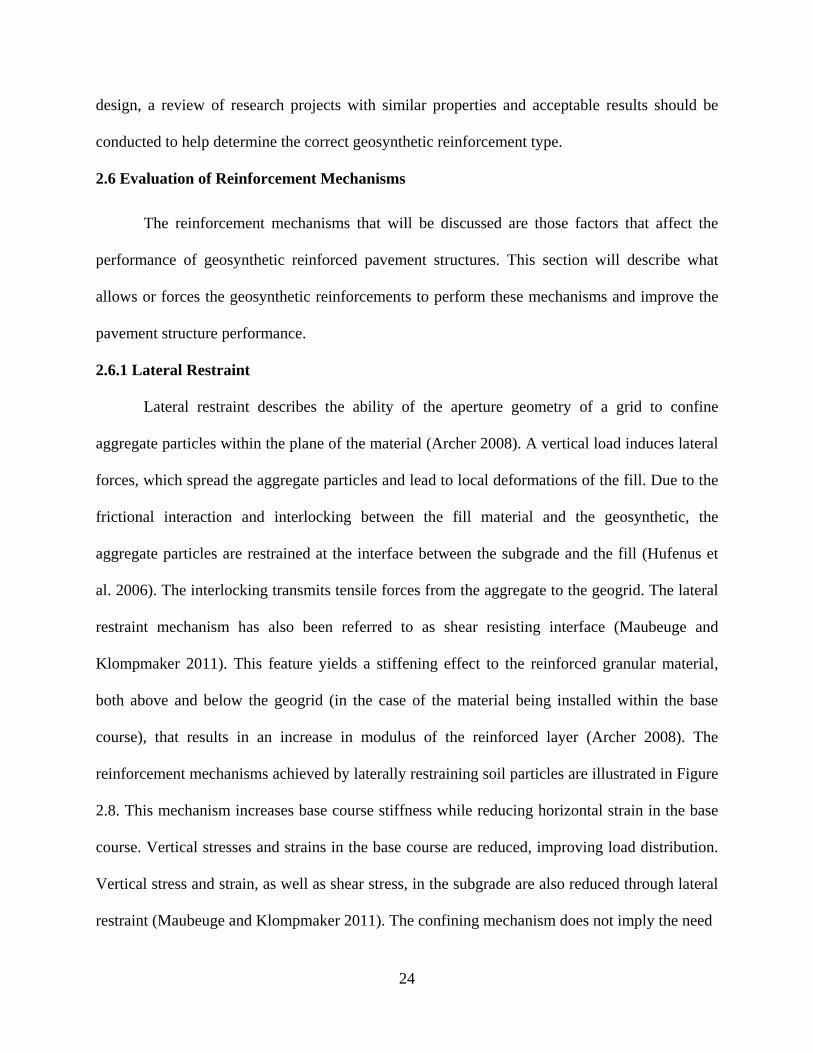
24
design, a review of research projects with similar properties and acceptable results should be
conducted to help determine the correct geosynthetic reinforcement type.
2.6 Evaluation of Reinforcement Mechanisms
The reinforcement mechanisms that will be discussed are those factors that affect the
performance of geosynthetic reinforced pavement structures. This section will describe what
allows or forces the geosynthetic reinforcements to perform these mechanisms and improve the
pavement structure performance.
2.6.1 Lateral Restraint
Lateral restraint describes the ability of the aperture geometry of a grid to confine
aggregate particles within the plane of the material (Archer 2008). A vertical load induces lateral
forces, which spread the aggregate particles and lead to local deformations of the fill. Due to the
frictional interaction and interlocking between the fill material and the geosynthetic, the
aggregate particles are restrained at the interface between the subgrade and the fill (Hufenus et
al. 2006). The interlocking transmits tensile forces from the aggregate to the geogrid. The lateral
restraint mechanism has also been referred to as shear resisting interface (Maubeuge and
Klompmaker 2011). This feature yields a stiffening effect to the reinforced granular material,
both above and below the geogrid (in the case of the material being installed within the base
course), that results in an increase in modulus of the reinforced layer (Archer 2008). The
reinforcement mechanisms achieved by laterally restraining soil particles are illustrated in Figure
2.8. This mechanism increases base course stiffness while reducing horizontal strain in the base
course. Vertical stresses and strains in the base course are reduced, improving load distribution.
Vertical stress and strain, as well as shear stress, in the subgrade are also reduced through lateral
restraint (Maubeuge and Klompmaker 2011). The confining mechanism does not imply the need

25
Figure 2.8. Lateral base course restraint (Maubeuge and Klompmaker 2011).
for significant rut depths to form and therefore is also of interest for permanent paved roads
(Hufenus et al. 2006).
2.6.2 Separation
Normally in roadways, a stiff material is placed over a soft material and when these two
materials intermix, the stiff material layer may decrease in thickness, creating a larger layer of
weak soil beneath a thin layer of stiff soil, as illustrated in Figure 2.9. This mixing of the layers is
known as fines migration. When this condition is present, separation is the most important
mechanism of the geosynthetic material. Al-Qadi et al. (1994) discovered that the separation
mechanism is more important in strengthening reinforced pavement sections than had been
reported previously in literature after excavating through test sections at the end of testing (Al-
Qadi et al. 1994). Studies performed on pavement reinforcement with geotextiles tend to show
that separation and filtration are the most important mechanisms for thin base course aggregate
thicknesses and weak subgrade conditions which are susceptible to fines migration (Fannin and
Sigurdsson 1996). Geotextiles are more effective at separation than geogrids.

26
Figure 2.9. Contribution of geotextile separation in pavements to prevent intermixing of layers (Berg et al. 2000).
2.6.3 Tensioned-Membrane Effect
If heavy traffic loads are applied to the base course surface and/or the subgrade is
extremely soft, significant deformations on the base course surface as well as on the subgrade
surface occur (Maubeuge and Klompmaker 2011). When geosynthetics are placed in heavily
trafficked roadways, predominantly unpaved roadways, the soil along the geosynthetic
reinforcement is able to deform enough to transfer enough stress to the geosynthetic to mobilize
tension, although this may require significant rutting (Giroud and Noiray 1981). The
configuration of the geogrid in such cases can be assumed as shown in Figure 2.10 (Maubeuge
and Klompmaker 2011). The geosynthetic reinforcement is stressed due to depression basin
created by the wheel path causing the geosynthetic to act as tensile support in the vertical
direction, reducing stresses applied to the subgrade and increasing bearing capacity. However,
high stiffness geosynthetic reinforcements along with large enough deformations to mobilize the

27
Figure 2.10. Tensioned membrane effect (Maubeuge and Klompmaker 2011).
geosynthetic are needed for the tensioned-membrane mechanism to be effective. Although,
punched and drawn geogrids are manufactured by “pre-straining” the polymer yielding an
effective stress transfer of vertical and horizontal stresses, mobilizing tensile resistance in both
woven and non-woven geotextiles requires strain to be induced after the product is installed,
which leads to rut accumulation in the base and subgrade layers before the geosynthetic actually
responds (Archer 2008).
2.7 Design Methods
Design methods for geosynthetic-reinforced pavements have been developed, but most
do not include many of the variables that impact pavement performance. The results gathered
through empirical studies are mixed; with some showing geosynthetics provide benefits to
pavement structures while some show there is no benefit. There are discrepancies between the
empirical studies that report there is a benefit because some claim geogrids perform better than
geotextiles, some claim they perform equally, and others claim that geotextiles outperform
geogrids. The empirical studies, therefore, reduce to gathering enough data to form an empirical

28
design method (Kinney et al. 1998). Empirical design methods are unable to account for
variations in the pavement configuration and geosynthetic type and placement. Due to the
variations in input parameters in flexible pavements, finite element design methods have been
created, but it is difficult to model the behavior of different soil types, geosynthetic behavior, and
the interactions between the two. These models are also limited to a response of the pavement
under a single load. Giroud and Han (2004) published a design method that combines bearing
capacity theory with empirical data from full-scale test sections and monitored unpaved roads
(Archer 2008). The Giroud and Han (2004) method considers: (1) the effects of variation in base
course strength, (2) the number and size of load cycles and the desired roadway performance, (3)
how the load distribution angle within the base course changes over time, and (4) recognition
that geogrids and geotextiles perform differently in roads and differently even from like
materials (Archer 2008). Giroud and Han (2004) state that the advanced design is theoretically
based and experimentally calibrated. Therefore, it more accurately predicts performance for both
geogrid and geotextile reinforced unpaved roads, and the new method supersedes the previous
methods from Giroud and Noiray (1981) and Giroud et al. (1985) (Giroud and Han 2004).
However, there is no specified and accepted design method even though geosynthetic materials
have been used to reinforce pavements for over 30 years. The lack of a standard design method
limits the growth of geosynthetic reinforcements being applied in flexible pavement structures.
2.8 Conclusion from Literature Evaluation
Many geosynthetic reinforced flexible pavement evaluations have been conducted. This
literature has referenced some of this work, but is not inclusive. There have been a number of
research efforts that display significant benefits to pavement performance brought by the
inclusion of geosynthetic reinforcements, such as Perkins and Cortez (2005), Al-Qadi et al.

29
(1994), and Cuelho et al. (2011). However, the amount and type of benefit are not typically
consistent from one study to the next. A few studies have shown little improvement from
including geosynthetic reinforcements in pavements, such as Cox et al. (2010a) and Henry et al.
(2011). These discrepancies seem to indicate that the problem is complex and many variables
need to be considered before simply assuming that placing geosynthetics in all pavement
structures will provide a cost-effective performance benefit. Henry et al. (2011) stated and
illustrated through data presentation that there could be a diminishing effect on the benefit
returns from the geosynthetic reinforcements as base course thickness increases. Geosynthetic
reinforcements have the potential to be greatly beneficial in flexible pavement structures with
poor subgrade soils or thin base course layers, but until there is consistency in research results
there will continue to be uncertainties in whether or not including geosynthetic reinforcements
will benefit specific flexible pavement structures and ultimately save money while improving the
service life of the road.

30
Chapter 3
3.0 Site History
3.1 Overview
In 2004, the Arkansas Highway and Transportation Department (AHTD) began
construction of a frontage road (Frontage Road 3) along US Highway 63 in the town of Marked
Tree, Arkansas at the intersection of Arkansas Highway 75. This frontage road was constructed
for a research project (AHTD TRC-0406). This field study was aimed at determining the
benefits, if any, of using geosynthetics for flexible pavement reinforcement on state funded
roadway projects. Typically, when poor subgrade soils are encountered, AHTD will over-
excavate and replace the poor material with quarried materials such as large crushed stone
(B-Stone) or standard road base (AHTD SB2-Class 7), depending on availability (Brooks 2009).
However, in many areas of the state with poor native soils, there are very few sources of quality
fill material within a reasonable distance, resulting in long hauling and costly pavements. The
native silt and clay subgrade soils in Northeast Arkansas have particularly poor engineering
qualities; therefore, it was hypothesized that the resulting benefits from geosynthetic materials
installed at the base and subgrade interface in a flexible pavement structure in this area would be
evident if these materials do, in fact, substantially enhance performance.
The initial objectives of TRC-0406 (referred to as the Marked Tree Project) were to: (1)
construct a full-scale flexible pavement with various configurations (i.e., base course
thicknesses, geosynthetic types, control sections, etc.), (2) instrument the pavement with strain
gauges, pressure cells, climate sensors, etc., (3) collect data from the instrumentation to infer the
mechanism(s) that most influence pavement performance, and (4) develop a finite element model

31
that could be used to predict critical structural responses of flexible pavements reinforced with
geosynthetics (Howard 2006). A profile view of the configuration of the pavement sections,
including type and location of instrumentation, is presented in Figure 3.1.
The original pavement configuration for the research consisted of 13, 50-ft (15-m) long,
10-ft (3.05-m) wide test sections (numbered 1 through 13 from east to west; refer to Figure 3.1).
Section 7 was constructed as a transition section that separated Sections 1-6, with 10-in (25-cm)
thick base layers, and Sections 8-13, with 6-in (15-cm) thick base layers. Sections 1 and 13 were
left unreinforced to act as control sections for each base thickness. Prior to construction, two
Mirafi geosynthetics (a geotextile and a geogrid) that were not initially planned were added to
the study. These two products were installed at each end of the pavement and were identified as
Sections 1A, 1B, 13A, and 13B (Warren and Howard 2007b). The geosynthetic configuration for
the first eight sections (Sections 1B – 6) is a mirror image of the configuration in the last eight
test sections (Sections 8 –13B) about Section 7. The specific types and manufacturers of the
geosynthetics installed in each section are provided in Figure 3.2. It must be noted that all
geosynthetics (including geogrids) were installed at the interface between the compacted
subgrade and the base course. No products were installed within the base. Furthermore, two
sections (Section 5 and Section 12) contained both a geogrid and a geotextile atop one another.
The soil properties and construction methods employed to create the Marked Tree
geosynthetic-reinforced pavement test sections will be explored in this chapter. The initial
conclusions drawn from the instrumentation and data processing involved with the original
research project (TRC 0406) will also be briefly summarized.

Figure 3.
Figure 3.al. 2010b
.1. Profile vi
.2. Schematib).
iew of instru
c of geosynt
umentation c
thetic reinfor
32
onfiguration
rced test sec
n (Warren an
ctions in Mar
nd Howard 2
rked Tree, A
2007).
Arkansas (Co
ox et

33
3.2 Site Description
The Marked Tree site consists of characteristically weak soils, which was the primary
reason for its initial selection for the geosynthetic reinforcement in flexible pavements project.
Weak subgrade soils plague the eastern side of Arkansas, making building efficient roadways
difficult. Geosynthetics can potentially improve the performance of low volume pavements in
such conditions by providing lateral restraint to the base course layer.
3.2.1 Site Location
The roadway under investigation is located in Marked Tree, Arkansas. Marked Tree is in
the northeastern portion of the state, approximately 33 miles south from Jonesboro, Arkansas and
38 miles north from Memphis, Tennessee. Figure 3.3 is a state map of Arkansas, which
highlights the county in which construction took place (Poinsett County). The test site is located
on Frontage Road 3, which serves to connect US Highway 63 and Arkansas Highway 75. Figure
3.4 is a vicinity map on which the test section has been denoted in red. At the time of
construction, Highway 63 was being converted into a controlled access roadway with interstate-
type on and off ramps as the only access points.
The sixteen test sections and the transition section are located between STA. 136+50 and
STA. 145+00 (850-ft [255-m] long) in the east-bound lane of Frontage Road 3 (the west-bound
lane was not part of the special instrumentation/construction plan). It should be noted that the
frontage road dead ends west of the testing site since it affects the traffic pattern of the roadway.
The topography of the test site is relatively flat. The majority of the land in the adjacent
areas is used for produce farming. Figure 3.5 is a picture of the test site prior to construction.
Marked Tree is a relatively small town located in an agricultural area with a population of
approximately 2,600. At the time of construction the majority of the traffic on Frontage Road 3

34
Figure 3.3. Arkansas state map featuring the project location.
Figure 3.4. Vicinity map of test site denoting approximate extent of test sections.
was anticipated from vehicles associated with the Arkansas State University Technical Center
located west of Section 13B (refer to Figure 3.4). However, a nursing home (Three Rivers
Nursing Center) was constructed just after completion of the road whose driveway intersects the
Section 13BSection 1B
N
Three Rivers Nursing Center
Arkansas State University Technical
Center

Figure 3.
testing ar
the 10-in
course se
3.2.2 Site
T
was initia
sampling
testing w
2009).
3.2.2.1 S
P
AHTD. T
time a se
.5. Test site p
rea between
n (25-cm) th
ections (Sect
e Character
There were tw
al sampling
g and testing
was used to c
Sampling and
rior to the ro
This explora
eries of twelv
prior to cons
Sections 7 a
ick base cou
tions 8 – 13B
rization
wo distinct p
and testing t
g took place
conduct inde
d Laboratory
oadway desi
ation occurre
ve borings w
struction (Ho
and 8. This u
urse sections
B) refer to C
phases in the
that was don
during the f
x and streng
y Testing
ign and cons
ed between S
were complet
35
oward 2006)
ultimately re
s (Sections 1
Chapter 4, Se
e characteriz
ne as part of
first attempt
gth testing to
struction, a s
September 8
ted. These tw
).
esulted in sl
1B – 6) than
ection 4.5.1).
zation of the
f the design p
to construct
o fully chara
subsurface e
8 and Septem
welve boring
Future RoaLocatio
ightly differ
n the 6-in (1
.
e onsite soils
process. The
t the roadwa
acterize the m
exploration w
mber 10, 20
gs each term
dway on
rent trafficki
5-cm) thick
s. The first p
e second rou
ay. This rou
materials (Br
was conducte
03, during w
minated at a d
ing of
k base
phase
und of
und of
rooks
ed by
which
depth

36
of 10-feet (3.05m) below existing grade, which varies from 2- to 4-feet (0.61- to 1.22-m) below
final top of subgrade for the completed roadway embankment. Each boring was located along the
centerline of the proposed road and spaced on approximately 50-feet (15.2-m) centers. Samples
collected during this exploration included both split spoon (disturbed) and Shelby tube
(undisturbed) samples (Brooks 2009).
A second set of borings was completed between October 5 and October 7, 2004. This set
of borings consisted of three holes within each planned test section: one for disturbed samples
(split spoon), one for undisturbed samples (Shelby tube), and one for bulk samples (auger
cuttings). There were 13 locations drilled at 50 feet (15.2 m) intervals along the centerline of the
road. These borings were drilled to a depth of 10 feet (3.05 m) below the rough finished grade of
the roadway earthwork after all necessary fill had been placed prior to blue-topping and final fine
grading of the roadway in preparation for the placement of geosynthetics and aggregate base
course (Brooks 2009). AHTD compiled final boring logs and extruded the Shelby tube samples
before transferring the packaged samples to the University of Arkansas in Fayetteville for
storage and subsequent testing. All extruded samples were carefully packaged and stored to
ensure preservation of moisture content. In-situ moisture contents were taken from the bag
samples. A composite soil profile based on all of the boring logs is presented in Figure 3.6. The
elevations in Figure 3.6 are in feet. Note that several more feet of compacted fill subgrade was
placed below the 6-in (15.2-cm) base course sections (Sections 8 – 13B) than below the 10-in
(25.4-cm) sections (Sections 1B – 6).
Laboratory testing was conducted on the samples to classify the soils as well as to
determine the strength and stiffness characteristics of the soils at each test section. Before testing,
the soil was processed to ensure all particles could pass through a #4 sieve. For classification

37
Figure 3.6. Subgrade soil profile based on Geotechnical exploration (Brooks 2009).
purposes, the soils were subjected to the following tests: Atterberg limits (ASTM D 4318-
00),Specific Gravity (ASTM D 854-02), and Particle Size Distribution (ASTM D 442-63). The
soils were classified according to both the USCS (ASTM D 2487) and AASHTO classification
systems. The index testing results and the soil classifications for Sections 1 – 13, excluding
Section 7, are provided in Tables 3.1 and 3.2 for USCS and AASHTO, respectively. Note that
classification information is not available for Sections 1B, 1A, 13A and 13B since those sections
were not planned at the time of site investigation. It can be seen that the site is very uniform in
terms of its soil classification (CH or A-7-6). Only Section 8 (station 141+25) classifies as CL.
Fines contents across these sections range from 67 – 90% and PI ranges from 35 – 53. The
plastic limit values are graphically presented in Figure 3.7. Nearly all sections had subgrade PI
ranging from 40 – 50, with only Sections 8 and 9 (slightly lower) and Section 13 (slightly higher)
falling outside this range.

38
Table 3.1. USCS soil classification of bulk samples from 2.5’ to 12.5’ (Brooks 2009).
Table 3.2. AASHTO soil classification (Brooks 2009).
The Shelby tube specimens from Sections 1 and 13 were divided into different zones as a
function of depth to represent the compacted subgrade, the upper natural ground, and the lower
natural ground. The in-situ dry density (unit weight) of the upper natural ground was 85 pcf
(1362 kg/m3), the lower natural ground was 95 pcf (1522 kg/m3), and the compacted subgrade
was 101 pcf (1618 kg/m3) (Howard 2006). The bulk samples collected during the second
subsurface investigation were used in Proctor testing to determine the maximum dry density and
optimum moisture content of the re-compacted subgrade soil at each section. The proctor tests
1 67 20 47 2.72 100 100 89.4 0 10.6 CH Fat Clay2 63 22 41 2.69 100 100 87.7 0 12.3 CH Fat Clay3 66 22 44 2.69 100 100 90.2 0 9.8 CH Fat Clay4 66 20 46 2.68 100 100 85.3 0 14.7 CH Fat Clay5 65 19 46 2.69 100 100 83.9 0 16.1 CH Fat Clay w/ Sand6 63 17 46 2.69 100 100 83.0 0 17.0 CH Fat Clay w/ Sand8 49 14 35 2.71 100 100 67.3 0 32.7 CL Sandy Lean Clay9 55 17 38 2.68 100 100 76.8 0 23.2 CH Fat Clay w/ Sand
10 60 17 43 2.67 100 100 83.6 0 16.4 CH Fat Clay w/ Sand11 61 18 43 2.71 100 100 85.7 0 14.3 CH Fat Clay12 62 17 45 2.71 100 100 87.8 0 12.2 CH Fat Clay13 73 20 53 2.71 100 100 89.0 0 11.0 CH Fat Clay
Group NameSection LL PL PISpecific Gravity
% Passing 3/4"
% Passing #4
% Passing #200
% Gravel % SandGroup
Symbol
1 2.5-12.5 Bulk 67 20 47 2.72 99.7 99.2 89.4 A-7-6 462 2.5-12.5 Bulk 63 22 41 2.69 99.9 99.4 87.7 A-7-6 393 2.5-12.5 Bulk 66 22 44 2.69 99.8 99.4 90.2 A-7-6 434 2.5-12.5 Bulk 66 20 46 2.68 99.9 99.2 85.3 A-7-6 435 2.5-12.5 Bulk 65 19 46 2.69 100 99.3 83.9 A-7-6 416 2.5-12.5 Bulk 63 17 46 2.69 100 99.1 83 A-7-6 408 2.5-12.5 Bulk 49 14 35 2.71 99.8 91 67.3 A-7-6 219 3.5-13.5 Bulk 55 17 38 2.68 99.9 99.6 76.8 A-7-6 2910 3.5-13.5 Bulk 60 17 43 2.67 100 99.6 83.6 A-7-6 3711 3.5-13.5 Bulk 61 18 43 2.71 100 99.5 85.7 A-7-6 3912 3.5-13.5 Bulk 62 17 45 2.71 99.9 99.5 87.8 A-7-6 4213 3.5-13.5 Bulk 73 20 53 2.71 100 99.4 89 A-7-6 52
Group Index
Section Depth (ft)Samply Type
LL PL PISpecific Gravity
% Passing #10
% Passing #40
% Passing #200
Group Class.

39
Figure 3.7. Plasticity index values of the subgrade from each section of the Marked Tree site from tests conducted in October 2004.
followed ASTM D 698-00 Method C. After a set of standard proctor tests were run on the soils,
it was determined that the maximum dry density was approximately 106 pcf (1698 kg/m3) and
the optimum moisture content was approximately 16.8% (Brooks 2009).
Additional laboratory tests were conducted on the compacted subgrade at Sections 1 and
13, such as California Bearing Ratio (CBR), resilient modulus (Mr) and unconsolidated
undrained (UU) triaxial tests. All these tests were, however, conducted on Proctor samples rather
than undisturbed samples that would more accurately represent the soil stiffness/strength in the
field. Mr values for Sections 1 and 13 ranged from approximately 11.0 – 15.8 ksi (75.8 – 108.9
MPa), undrained shear strengths (Su) ranged from approximately 2.91 – 5.36 ksi (18.9 – 37.0
MPa), and CBR values ranged from 1.38 to 1.66, but could be expected to reach a minimum of
0.8 (Brooks 2009). The processes for conducting these tests, as well as the results, can be found
in greater detail in Howard (2006) and Brooks (2009).
0
10
20
30
40
50
60
1 2 3 4 5 6 7 8 9 10 11 12 13
Pla
stic
ity
Inde
x, P
I
SectionT
ran
siti
on S
ecti
on

40
3.3 Site Construction
The research team for the initial Marked Tree project (TRC 0406) originally traveled to
the site and installed earth pressure cells in the finished subgrade in October of 2004.
Unfortunately, harsh winter weather prevented completion of the roadway, forcing all subgrade
sensors to be removed to allow the subgrade surface to be re-worked in June of 2005.
The following subsections discuss the construction techniques for completing the
geosynthetic-reinforced and instrumented eastbound lane of Frontage Road 3. Unfortunately, the
original work described in Howard (2006) did not mention the geosynthetics that were installed
in the westbound lane. It was known from construction photographs that a single type of
geosynthetic was installed at the interface of the compacted subgrade and base in the westbound
lane, however, the type of geosynthetic was not known. It was discovered in an October 2010
forensic exploration of the westbound lane adjacent to Sections 13 and 13B that the westbound
lane was reinforced with a Carthage Mills woven, slit film geotextile (FX-66). This geotextile
was installed over the entire width of the westbound lane and overlapped into the eastbound lane
approximately 3 feet (0.91 m). Figures 3.8 and 3.9 are construction pictures displaying the
overlapping of the Carthage Mills geosynthetics from the westbound lane to the eastbound lane.
This overlap only left approximately 9 feet (2.74 m) of the eastbound lane from the south edge of
the roadway (the right wheel path) to observe the effects of the geosynthetics installed in the 16
different eastbound lane test sections.
3.3.1 Subgrade
As previously noted, the subgrade was prepared in October of 2004, but winter weather
prevented completion of the roadway and the subgrade had to be reworked in June of 2005. The
re-work consisted of removal of the top few centimeters of the subgrade and re-compacting new
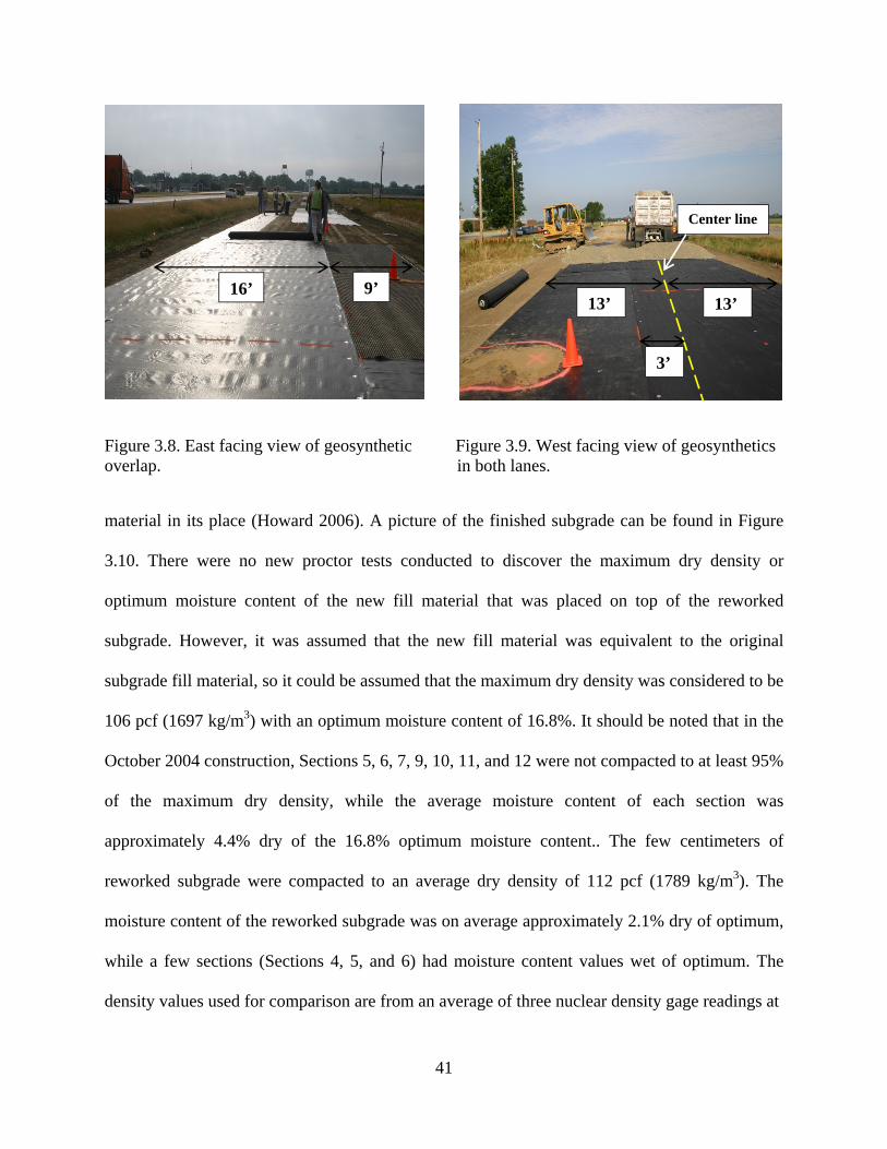
41
Figure 3.8. East facing view of geosynthetic Figure 3.9. West facing view of geosynthetics overlap. in both lanes.
material in its place (Howard 2006). A picture of the finished subgrade can be found in Figure
3.10. There were no new proctor tests conducted to discover the maximum dry density or
optimum moisture content of the new fill material that was placed on top of the reworked
subgrade. However, it was assumed that the new fill material was equivalent to the original
subgrade fill material, so it could be assumed that the maximum dry density was considered to be
106 pcf (1697 kg/m3) with an optimum moisture content of 16.8%. It should be noted that in the
October 2004 construction, Sections 5, 6, 7, 9, 10, 11, and 12 were not compacted to at least 95%
of the maximum dry density, while the average moisture content of each section was
approximately 4.4% dry of the 16.8% optimum moisture content.. The few centimeters of
reworked subgrade were compacted to an average dry density of 112 pcf (1789 kg/m3). The
moisture content of the reworked subgrade was on average approximately 2.1% dry of optimum,
while a few sections (Sections 4, 5, and 6) had moisture content values wet of optimum. The
density values used for comparison are from an average of three nuclear density gage readings at
16’ 9’13’ 13’
Center line
3’

Figure 3.
each sec
displayed
3.3.2 Geo
T
a strong j
separatio
the base
In
loading.
the geos
geosynth
gages we
.10. Finished
ction. The d
d versus Sec
osynthetics
The geosynth
justification
on effect whe
course may
nstrumentati
The goal of
synthetics in
hetics in the
ere attached,
d cut subgrad
density value
tion in Figur
hetics were in
for putting t
en placed be
not be suffic
ion was attac
f this instrum
n the pavem
laboratory a
several prov
de (Howard
es from both
re 3.11.
nstalled at th
the geosynth
etween two
cient to obta
ched to the
mentation wa
ment structu
and subsequ
visions were
42
2006).
h dates are
he subgrade
hetics at this
layers, but t
in a benefit
geosyntheti
as to infer th
ure. Foil-ty
uently transp
e necessary t
provided in
and base co
s depth. Wov
the interactio
(Berg et al. 2
cs to infer t
he level of im
ype strain g
ported to the
to prevent da
n Table 3.3
ourse interfac
ven geotextil
on between
2001).
the strains in
mprovement
gages were
e constructio
amage to the
3 and graphi
ce. There wa
les will prov
the geogrid
nduced by tr
t gained by u
attached to
on site. Onc
e instruments
ically
as not
vide a
ds and
raffic
using
o the
ce the
s
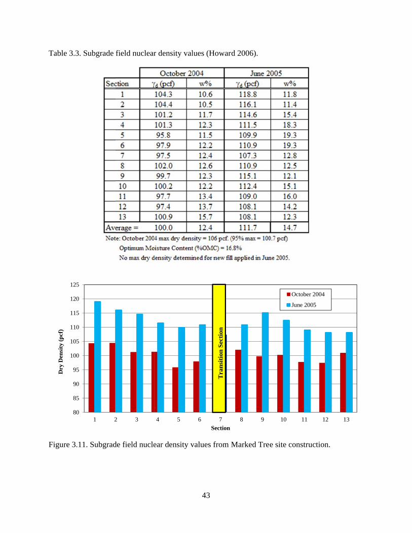
Table 3.3
Figure 3.
80
85
90
95
100
105
110
115
120
125
Dry
Den
sity
(p
cf)
3. Subgrade
.11. Subgrad
0
5
0
5
0
5
0
5
0
5
1 2
field nuclear
de field nucle
2 3
r density val
ear density v
4 5
43
lues (Howard
values from M
6 7
Section
Tra
nsi
tion
Sec
tion
d 2006).
Marked Tree
8 9
e site constru
10 11
Octobe
June 20
uction.
12 13
er 2004
005
3

44
during transportation and installation (Brooks 2009). The instrumented geogrids were rolled
from each end in a scroll-like fashion to make field alignment easier. By rolling each end to the
center, the grid could be unrolled by first aligning the gage with its proper location on the
subgrade. Geotextiles were also folded so that the active gage could easily be aligned to the
proper location on the subgrade (Howard 2006).
Placement of each of the 56-ft (17.1-m) long geosynthetics was performed with care to
ensure quality control and assurance. All geosynthetics were tensioned and placed on a smooth
surface, free of wrinkles, using methods that simulated typical installation. It was necessary to
locate the active geosynthetic strain gage within 1.2 inches (30mm) and prevent movement of the
gage while the remainder of the geosynthetic was placed without reinforcing the area local to the
gage. The procedure was developed entirely due to the instrumentation. Such a complicated
procedure would not be practical or commonplace in construction. A typical installation would
consist of rolling the material onto the subgrade relatively free of wrinkles and possibly tacking
it into place (Howard 2006).
The following procedure was developed by Howard (2006) for the installation and
protection of the instrumented Propex 2006 and Propex 2044 geotextiles. This procedure utilized
nine people and two trucks. In addition to the planned protection measures, sand placed during
earth pressure cell installation was present and provided a cushion for the gages. The following
terms are commonly reoccurring during the procedure explanation, so to prevent from
unnecessary repetition they are defined as follows:
Pins: Standard U-shaped landscaping pins approximately 6 inches (150 mm) long. Pipe: 4-inch (10.2-cm) sewer and drain (S/D) pipe that was slightly longer than the
widest geosynthetic.

45
Tensioner: Two wooden boards were fastened together with the top half of an S/D pipe attached to it. The composite board extruded form one truck tailgate to the other and had cross sectional dimensions of 3.0 x 5.6 inches (76 x 140 mm). The geosynthetic rolled over the top of the composite board during the tensioning process so the top half of the S/D pipe provided a smooth surface and prevented the geosynthetics from catching on bare wood (see Figure 3.12).
Installation method as defined in Howard (2006):
1) Locate the active gage over the center of the subgrade earth pressure cell and either unroll or unfold the entire geosynthetic.
2) Use standard surveying equipment to align the active geosynthetic strain gage and earth pressure cell center to within at most 1.2 in (30 mm).
3) Pull laterally (perpendicular to the traffic direction) on the geosynthetic at the gage location to remove all wrinkles and hold the material taunt while driving six pins uniformly across the width of the geosynthetic, ensuring all pins are at least 12 inches (300 mm) from the gages.
4) Place full buckets of sand behind the gages to help them remain stationary.
5) Measure and place a mark every 8 feet (2.44 m) on the geosynthetic on both sides of the gage. These marks will be used for pin placement in the geosynthetics.
6) Tension one side of the test material with reference to the gage. Slide the tensioner under the side of the geosynthetic being installed.
7) Position the two trucks as seen in Figure 3.12.
8) Persons 1 and 2 on Figure 3.12 straighten the geosynthetic, and then stand on the corners as shown, with persons 3 and 4 off the geosynthetic.
9) Persons 3 and 4 then walk toward the tensioner until enough force is present to start to lift the pipe with person 8 standing on it.
10) Once tension is applied, person 8 directs the trucks to pull forward very slowly and persons 7 and 9 roll the pipe forward at the same rate that the trucks move forward. During the lay down process, person 8 is ensuring adequate tension is maintained by adjusting the position of persons 3 and 4, controlling the rate of the trucks and pipe personnel to keep the geosynthetic straight and going under the pipe at an angle of approximately 450, and removing wrinkles from the geosynthetic as it traverses over the tensioner.

46
Figure 3.12. Geosynthetic tensioning technique (Howard 2006).
11) The process was continued until the first 8-ft (2.44-m) interval was reached. At this juncture, the lay down process was halted and persons 5 and 6 placed six pins equally across the geosynthetic.
12) The process was then repeated two more times, which left approximately 4 feet (1.2 m) of loose material at each end. The procedure was performed on both sides of the gage, beginning at the gage and traveling away from this area in the longitudinal direction.
13) The 4 feet (1.2 m) of loose material on either end overlapped the adjacent test section by
3 feet (0.91 m). The overlaps were pulled taunt by hand and six pins were placed equally across the geosynthetic. The laps were oriented so that when aggregate was bladed laterally onto the geosynthetics, the material would not tend to roll up.
14) Once the geosynthetics were installed, measures were taken to protect the foil strain
gages during construction and service. For example, the cables were arranged to provide stain relief and the geogrid and geotextile strain gages were covered prior to testing. Figure 3.13 shows the small portion of the inverted core of a standard strip drain used to protect the geogrid strain gages, and Figure 3.14 shows the neoprene pads that were utilized to protect the geotextile strain gages. The cables were covered with fine sand (Figure 3.15) and crushed stone was then hand placed over the sand to a depth of approximately 6 in as seen in Figure 3.16.

47
Figure 3.13. Geogrid strain gage protection, strip drain (Howard 2006).
Figure 3.14. Geotextile strain gage protection, neoprene pad (Howard 2006).
Figure 3.15. Sand covering geosynthetic strain gage and cable (Howard 2006).

48
Figure 3.16. Crushed stone covering fine sand, geosynthetic strain gage, and cable (Howard 2006).
A modified version of the aforementioned procedure was utilized for the instrumented
Tensar BX 1200 geogrids and Propex 4553 geotextiles. Steps 7) – 10) were omitted, and the lay
down process was performed entirely by hand. The Propex 4553 could manually be pulled taunt
due to the increased deformation ability of the material, and the BX 1200 could be placed in the
same orientation regardless of the lay down procedure (Howard 2006).
3.3.3 Base Course
Crushed stone aggregate was used for the construction of the base course. The properties
of the crushed stone used for the construction can be found in Table 3.4. These values were
obtained from Howard (2006). It should be noted that there is uncertainty about when and where
throughout the testing site the average nuclear density gage values for dry unit weight were
collected.
The base course was constructed by placing aggregate on the non-instrumented lane to
provide a working platform next to the instrumented subgrade and geosynthetics. Aggregate was
placed to a depth sufficient to obtain the first 6-inch (150-mm) lift of compacted material on both
lanes (Figure 3.17). Once sufficient material was present along the entire test section, aggregate
was laterally bladed onto the test sections as shown in Figure 3.18. Until aggregate covered the
instrumented test sections, all sensitive areas were continuously marked with fluorescent paint

Table 3.4
Figure 3.
4. Crushed st
.17. Base cou
tone propert
urse placem
ties (Howard
ent on non-i
49
d 2006).
instrumentedd lane (Howaard 2006).
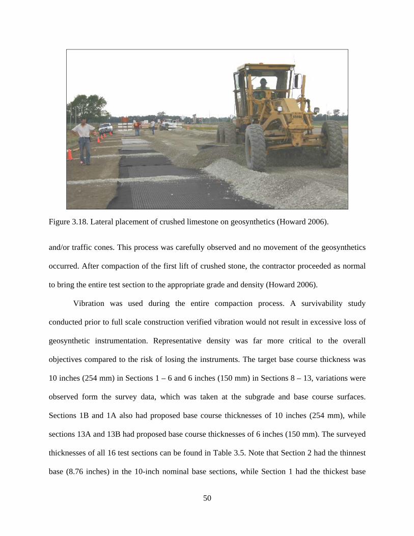
50
Figure 3.18. Lateral placement of crushed limestone on geosynthetics (Howard 2006).
and/or traffic cones. This process was carefully observed and no movement of the geosynthetics
occurred. After compaction of the first lift of crushed stone, the contractor proceeded as normal
to bring the entire test section to the appropriate grade and density (Howard 2006).
Vibration was used during the entire compaction process. A survivability study
conducted prior to full scale construction verified vibration would not result in excessive loss of
geosynthetic instrumentation. Representative density was far more critical to the overall
objectives compared to the risk of losing the instruments. The target base course thickness was
10 inches (254 mm) in Sections 1 – 6 and 6 inches (150 mm) in Sections 8 – 13, variations were
observed form the survey data, which was taken at the subgrade and base course surfaces.
Sections 1B and 1A also had proposed base course thicknesses of 10 inches (254 mm), while
sections 13A and 13B had proposed base course thicknesses of 6 inches (150 mm). The surveyed
thicknesses of all 16 test sections can be found in Table 3.5. Note that Section 2 had the thinnest
base (8.76 inches) in the 10-inch nominal base sections, while Section 1 had the thickest base

51
(11.58 inches). In the 6-inch nominal base sections, Section 10 had the thinnest base (5.64
inches), while Section 13B had the thickest base (6.72 inches).
Hand tools were used to excavate all holes and trenches necessary for base course sensor
and cable placement. As in the subgrade, the entire base course was finished before any sensors
were installed. Instrument locations were determined using standard surveying equipment to
allow precise alignment with the previously installed subgrade sensors (Howard 2006).
3.3.4 Asphalt Layer
The design asphalt thickness was 2 inches (51 mm) in all test sections, and the entire
pavement was surface course (0.5 in (12.7 mm) Superpave mix), placed in a single pass of the
paving train. The asphalt strain gages and thermocouples were installed at locations determined
using standard surveying equipment prior to paving. Paving modifications were necessary to
avoid damage to these sensors while still producing a quality asphalt mat. The instrumented test
sections were located in the middle of the frontage road so the contractor pave normally until the
instrumented sections were approached (Howard 2006). Once the instrumented sections were
reached, the paving train was stopped until sufficient asphalt was present to pave the entire
length of the one lane research section. This process required approximately nine trucks. The
paving train consisted of the following: 1) the truck hauling the asphalt, 2) shuttle buggy (Road
Tec 74-001 SB-25 00B), 3) paver (Cedaraphids CR 461R), 4) breakdown roller (Ingersol Rand
DD-138 steel wheel roller), and 5) finish roller (Ingersol Rand DD-130 steel wheel roller). To
avoid the sensors located in the outer wheel path, the tires of the shuttle buggy drove within a
few centimeters of the outside of the asphalt patch containing the sensors, and the loaded trucks
pulled around the buggy from behind, and subsequently backed up to it to unload. The paver was
also shifted and straddled the asphalt patches so that the tracks narrowly missed the strain gages.

52
Table 3.5. As-built base course surveyed thicknesses.
The roller pattern used for the test sections consisted of an initial single static pass with the
breakdown roller followed by three vibratory passes with the breakdown roller and finally two
static passes with the finish roller (Howard 2006).
As-built asphalt thickness values were observed using surveying techniques, as well as by
extracting cores between test sections. The thickness values obtained from the extracted cores
can be found in Table 3.6. The core thickness values reported were the average of readings taken
at quarter points with a digital caliper. The survey data was determined unreliable due to its
variability, lack of agreement with the extracted asphalt cores, and lack of agreement with the
design asphalt thickness of 2 inches (51 mm). For some reason, Sections 1B, 1A, 13A, and 13B
(mm) (in)
1B 280.42 11.041A 283.46 11.161 294.13 11.582 222.50 8.763 231.14 9.104 242.57 9.555 250.70 9.876 232.66 9.16
Transition 7 - -8 167.89 6.619 167.89 6.6110 143.26 5.6411 162.56 6.4012 160.27 6.3113 165.10 6.5013A 161.54 6.3613B 170.69 6.72
1. Base course thicknesses come from page 5-6, Table 5.1, in Warren and Howard (2007b).
Section Surveyed Thickness1
10" Nominal
Base Thickness
6" Nominal
Base Thickness

53
all had asphalt thicknesses less than 1.5 inches. No other sections had asphalt thicknesses less
than 2 inches.
3.4 Instrumented Testing Results (Summary)
The Marked Tree testing site was constructed to assess field performance of a flexible
pavement structure reinforced with geosynthetics through instrumented test sections. The goal
was to test the pavement over a wide range of temperature and moisture conditions with an
emphasis on performance during the weakest (higher moisture content) conditions (Howard
2006). However, due to unusually dry conditions during the months leading up to and during
testing, the expected benefits of the geosynthetics for wet conditions were not observed, making
a true assessment of their benefits based on measured responses inconclusive. A post
construction study also observed that only 77% of the installed environmental sensors provided
functional signals and only 82% of the structural sensors were functional (Warren and Howard
2007b). These survival rates were considered acceptable when considering the harsh construction
and environmental conditions the instruments were subjected to. There were water content
probes installed that were deemed unreliable and the thermocouples were very problematic. Due
to unexpected weather, harsh conditions, and time constraints the instrumented sections were
only observed for approximately 6 months.
The original testing of this site was intended to be under normal traffic conditions for a
year, but the construction of a nursing home on the land adjacent to this site with a driveway
intersecting Section 8 caused the research team to accelerate the data collection to ensure the
results of the study were not compromised by irregular traffic patterns from the nursing home.
AHTD kept the frontage road closed to traffic until the construction of the nursing home was
complete to provide a controlled testing environment for the accelerated testing process. AHTD

54
Table 3.6. As-built asphalt core thicknesses.
provided a dump truck for trafficking the site continuously for four one-week test intervals
between September 2005 and March 2006 (Warren and Howard 2007b). Due to the dry
conditions, the subgrade remained near optimum conditions, therefore the geosynthetic strain
gages were unable to measure meaningful data; however, the asphalt strain gages and earth
pressure cells provided reasonable results from the dynamic loading.
It was concluded that data acquisition methodology was successfully applied in a full
scale test, and independent test section triggering was shown to be plausible and efficient.
However, due to the dry conditions and variability in construction, the desired assessments of
test section performances were made inconclusive from a practical standpoint. There was
agreement in the measured stress and strain responses in comparison to calculated values for the
overall test section. Unfortunately, the data could not be utilized for section to section
(mm) (in)
1B 280.42 11.041A 283.46 11.161 294.13 11.582 222.50 8.763 231.14 9.104 242.57 9.555 250.70 9.876 232.66 9.16
Transition 7 - -8 167.89 6.619 167.89 6.6110 143.26 5.6411 162.56 6.4012 160.27 6.3113 165.10 6.5013A 161.54 6.3613B 170.69 6.72
1. Asphalt thicknesses come from page 118, Table 5.2, in Howard (2006).
10" Nominal
Base Thickness
6" Nominal
Base Thickness
Section Core Thickness1

55
comparisons (Howard 2006). The most significant conclusion drawn in Howard (2006) would
seem to be that the geosynthetic contributions were not evident. However, this conclusion was
based on limited testing data at a site with uncharacteristically dry conditions. Howard (2006)
recommended that it would benefit researchers to continue monitoring the instrumented test site
for several years to eliminate the variability of unusually dry and/or wet seasons and capture
representative conditions before absolute conclusions could be drawn. The conclusions
discussed, as well as many others, can be found in Howard (2006), Warren and Howard (2007a),
and Warren and Howard (2007b).

56
Chapter 4
4.0 Project Continuation
4.1 Overview
After limited observations and inconclusive results, the original Marked Tree research
project, AHTD TRC 0406, came to a halt in the Spring of 2006. In the Fall of 2007, Dr. John
McCartney and Dr. Brady Cox proposed to continue studying the Marked Tree site. This
proposal was accepted with the project number AHTD TRC 0903 and a start date of July 2008.
Their initial plan was to continue collecting data from the original instrumentation under both
normal traffic and accelerated loading, and to supplement this data with other non-destructive
testing methods for two years. Unfortunately, when the new research team arrived at the site in
July of 2008, virtually all of the instrumentation, with the exception of the asphalt strain gauges,
was no longer functioning. The dead instrumentation led the research group to rely on results
collected from numerous non-intrusive surficial load tests and observations from a more recent
internal investigation of each section obtained through forensic excavation. Later in this chapter,
a summary of the tests conducted at the site will be presented. These test methods and results
will be discussed in greater detail in the following chapter (Chapter 5). This chapter will also
discuss the pavement condition as defined by distress surveys conducted by AHTD in June of
2010 and April of 2011, as well as the estimated traffic loading this road has been subjected to
since construction ended in 2005.
4.2 Introduction
Although many researchers indicate that geosynthetic reinforcement leads to improved
pavement performance (refer to Chapter 2), a field or laboratory test has not been identified to

57
consistently quantify the contribution of the geosynthetic to the pavement’s overall performance.
Accordingly, there is little experimental evidence to guide the optimal location of the
geosynthetic, selection of the best geosynthetic for use in different situations (i.e., environmental
conditions, subgrade materials, etc.), and indication of what soil and geosynthetic properties best
indicate an improvement in pavement performance. The Marked Tree, AR site for TRC 0406 is a
very unique site due to variable geosynthetics and base course thicknesses resting on very poor
quality subgrade material. Originally, the site was also instrumented with multiple sensors
installed to measure deformation, moisture content, temperature, precipitation, and earth pressure
(Figure 3.1, Chapter 3).
However, the site was only monitored for a short time without significant traffic or
weather changes and limited conclusions were drawn from this full-scale test site with such
unique conditions. The goal of TRC 0903 was to continue the instrumentation monitoring of the
different test sections and to determine global stiffness and modulus values for each section as a
whole, and within each layer of the sections, respectively. This site provides a unique
opportunity to assess the mechanisms of geosynthetic reinforcements in flexible pavements and
to determine the relative importance of separation, lateral restraint, drainage, and base course
thickness on pavement performance.
4.3 Initial Objectives of TRC 0903
The overall objective of TRC 0903 was to investigate the mechanisms of geosynthetic
reinforcements installed in flexible pavements for low volume roads and to evaluate different
field tests to infer the contribution of geosynthetic reinforcement to overall pavement
performance. Additional goals of this study included direct comparison of the performance of
various geosynthetic types used for reinforcement at the Marked Tree site (seven different
58
products were used) and evaluation of the pavement geometry (two different base course
thicknesses were used). The initial, specific objectives of this study were as follows:
Objective 1: Review and re-interpret available information regarding soil and geosynthetic properties, pavement geometry, instrumentation layouts, and performance data (i.e. deflection basins from FWD testing) from TRC 0406, and develop a framework for comparison of the initial pavement performance with the current and future pavement performance.
Objective 2: Evaluated the current performance of the pavement test sections at the Marked Tree site; including visual pavement inspection (survey, cracking, rutting profiles, etc.), instrumentation assessment (survivability and calibration of existing sensors), and data acquisition system evaluation. A secondary objective would be to collect soil samples for additional hydraulic and mechanical assessment in the laboratory to complement field studies.
Objective 3: Re-start long-term monitoring program of the pavement test sections using instrumentation originally installed at Marked Tree site in order to evaluate the performance of the sections under normal vehicle traffic and environmental changes. Incorporate additional capacitance sensors in the roadway shoulder to better capture patterns in moisture content fluctuations in the subgrade.
Objective 4: Perform field measurements (dynamic and static) to determine the “global” performance of reinforced and unreinforced pavement test sections. Determine the global moduli using additional surface sensors (geophones) and the stress distributions and strain magnitudes using existing embedded sensors (strain gauges and pressure cells) under static and dynamic loads from a vibroseis truck. Consider the impacts of different surface loads (magnitude and frequency) and weather conditions.
Objective 5: Perform field measurements (dynamic) to determine the “individual” pavement layer moduli (compression and shear) in the reinforced and unreinforced pavement sections using shallow seismic borehole tests (crosshole and downhole) in non-critical areas of the pavement. Use the information gained from such testing along with visual inspection of boring data to consider the impacts of lateral restraint, separation, water content, and drainage conditions on layer moduli.
Objective 6: Evaluate results from the long-term monitoring program, global and individual layer moduli measurements in the pavement test sections, and comparisons of the performance of different test sections to draw conclusions with respect to the mechanisms of geosynthetic reinforcement (lateral restraint, pumping and fine particle migration due to cyclic increases in pore water pressure, aggregate intrusion into the subgrade, and moduli changes due to moisture flow).
Objective 7: Use comparisons between unreinforced and reinforced pavement test sections to perform a life-cycle cost analysis and develop specifications for using different types of geosynthetic reinforcements and pavement geometries.

59
Unfortunately, the objectives of this project had to be significantly adjusted once it was
discovered that nearly all of the instrumentation previously installed was dead on arrival to the
site. This prevented the group from continuously studying the long-term and seasonal effects on
the test sections through the abundance of instrumentation. However, there has been extensive
surface and subsurface testing and data collection and reduction conducted on the reinforced and
unreinforced flexible pavement test sections. The following section will include a summary of
the testing history from the current day back to the early FWD testing conducted in 2005.
4.4 Testing History
Surficial deformation and subsurface strength/stiffness tests have been conducted on the
Marked Tree site as far back as September of 2005 to as recently as May of 2011. A summary of
the dates and types of tests conducted is presented in Table 4.1. It should be noted that on some
of the dates for a few of the tests, only 8 sections were tested (1B, 1A, 1, 5, 9, 13, 13A, and 13B)
out of 16 possible sections, represented by a “5” in Table 4.1. These 8 sections were chosen
because the research group first wanted to concentrate on the following major reinforcement
configurations for both the 10-in (25-cm) and 6-in (15-cm) proposed base course thicknesses:
geotextile, geogrid, unreinforced, and geotextile/geogrid composite. The data collected for the
tests only conducted on 8 sections was not included in the final evaluation of the pavement test
section performance (refer to Chapter 5) because eventually all 16 test sections were evaluated
on a regular basis.
Cells in Table 4.1 that are labeled with a “1” represent tests that were conducted on all 16
test sections with data collected and reduced to analyze and compare relative pavement section
performance. Cells that are numbered “3” or “4” represent tests that did not produce interpretable
data and therefore were not included in the final analysis and ranking. As shown in the table,

60
Spectral Analysis of Surface Wave (SASW) testing was conducted at the Marked Tree site on
three dates, however, that data will not be presented in this study. Some of the SASW results are
presented by McCartney et al. (2011). The tests displayed in Table 4.1 only include deflection
and strength/stiffness tests conducted at the Marked Tree site.
The FWD testing conducted in 2005 and 2006 was analyzed in Howard (2006) using a
simple global modulus equation, but for this analysis, the calculated results were discarded and
the raw deflection data was re-analyzed using methods that will be discussed in Chapter 5. All of
the types of tests presented in Table 4.1, excluding SASW, will be discussed in Chapter 5.
4.5 Pavement Condition
The Marked Tree test site was constructed on a very low volume frontage road (Frontage
Road 3) that runs parallel to Arkansas Highway 63. It was finished in September of 2005. In July
of 2008, the pavement appeared to be in fairly good condition, with cracking and rutting limited
to small areas directly above sensor locations at the center of each test section. This deformation
appeared to be the result of relatively poor compaction around sensors and cables, which resulted
in pavement compression over time. However, the pavement began to deteriorate during the life
of the project and some areas in the westbound lane had rutted and cracked to “failure” [defined
as rutting over 0.5 inches(1.3 cm)] by the Spring of 2010. A couple of the test sections in the
eastbound lane also showed significant distress at this time (Section 10 in particular, which had
the thinnest surveyed base course, as reported in Section 3.3.3). The cracking present in the test
sections in the eastbound lane was determined to primarily be the result of the roadway
construction (longitudinal cracks at the centerline), temperature effects (transverse cracking), and
deformation immediately around sensor locations at the center of each test section (some limited
alligator cracking). However, the rutting was deemed a result of traffic loading on a pavement

61
Table 4.1. Summary of deflection and strength/stiffness tests conducted at Marked Tree site.
structure constructed on poor subgrade soils. Traffic counts have been conducted at the test site
that allow for a calculated estimate of the loads that have been applied to this road since
construction. Distress surveys were also conducted in June of 2010 and April of 2011 that allow
for developing a quantitative performance assessment for each test section.
4.5.1 Traffic Loading
The Arkansas Highway and Transportation Department (AHTD) has provided the
research team with traffic volume data from a somewhat continuous traffic count starting on
January 4, 2011 and continuing through August 31, 2011, excluding April 1, 2011 through May
26, 2011. The traffic volumes collected from these counts were analyzed and Equivalent Single
Axle Loads (ESALs) per year were calculated/estimated for eastbound (EB) and westbound
(WB) traffic at two different counter locations (East Counter and West Counter). The calculated
ESALs per year for each counter and direction are provided in Figure 4.1. The two traffic
counter locations were chosen so that the differences in ESAL’s between Sections 1B-8 and
Sections 9-13B could be obtained, recalling that the driveway for the nursing home intersects the
2005 - 2006 July 2008 Dec 2008 Jan 2009 May 2009 Dec 2009 Oct 2010 May 2011
FWD 1 & 2 1 1 1 1SASW 5 5 5PLT 3 5 5 1ADD 3 4 5 1 1DCP 1 1In-Situ CBR 1LWD 1Res Mod/UU 1RDD 11. Testing conducted in all sections.2. Testing Conducted four different times on the following dates: 9-13-05, 9-29-05, 12-20-05, 2-16-06.3. Tests conducted over sensor locations; poor data, could not be interpreted.4. Irregular ground force, data could not be interpreted.5. Only tested Sections 1b, 1a, 1, 5, 9, 13, 13a,13b
Test TypeDate

62
test sections within Section 8. Interestingly, this location almost perfectly split the 10-in (25.4-
cm) base course sections from the 6-in (15.2 cm) sections, with part of Section 8 being the only
6-in (15.2-cm) section more heavily trafficked than the rest. Note that Sections 1B-8 received
more than twice as many ESAL’s per year (approximately 6,600) as Sections 9-13B
(approximately 3,200).
The traffic data from AHTD was broken down into ten vehicle classifications, ranging
from motorcycles to six or more axle single trailers. There was some uncertainty associated with
how the absolute number for each classification was obtained, but the total traffic volume was
considered reliable. The initial task was to calculate the total volume at each counter location,
excluding motorcycle traffic. Then, with the classification totals calculated at the East Counter
for the westbound direction (i.e., all incoming traffic); a percent of contribution to the total
volume was calculated for each of the remaining nine classifications. Once that was calculated, a
truck factor for each vehicle classification was calculated.
The truck factor was calculated using Load Equivalency Factors (LEF) from Table 20.3
in Garber and Hoel (2001). Since actual loads were not known for each axle configuration on
each vehicle, a range of 12,000 to 20,000 lbs was used for single axles and a range of 16,000 to
32, 000 lbs was used for tandem axles. With these load ranges, there was a high and low LEF for
each vehicle classification that was considered a truck. The truck factors for each vehicle
classification were calculated by adding up the product of the number of each axle type per
vehicle with the LEF for that certain load and axle type. The vehicle classifications and truck
factors for each vehicle classification are displayed in Table 4.2.

63
Figure 4.1. Estimated ESALs per year.
Once a truck factor was assigned to each vehicle for the high axle loads and the low axle
loads, the respective truck factors were multiplied by the percent of contribution each
classification had on the total volume calculation. The products were considered “weighted”
truck factors that were then added together to create a “cumulative” truck factor for the high axle
load condition and the low axle load condition. The cumulative truck factors were then
multiplied by the total volumes at each counter (East and West) for each direction (EB and WB)
to produce estimated ESAL values per year from the 159 day count. Since there was a high and
low axle load condition, the high and low ESAL values were averaged for all four counting
locations. These averages were finally factored to represent an estimated yearly ESAL value for
each location, which are displayed in Figure 4.1. These ESAL values were deemed to be
reasonably close to the design traffic loading values for this type roadway.
N
East Counter (ESALs/year):
EB: 6660
WB: 6598
West Counter (ESALs/year):
EB: 3192
WB: 3168
Section 8

64
Table 4.2. Truck factors for each vehicle classification.
4.5.2 Distress Survey
AHTD conducted distress surveys on every test section at the Marked Tree site in June of
2010 and April of 2011. These distress surveys allow the pavement condition/performance to be
quantified. While rut depth in each wheel path, percent alligator cracking, and total longitudinal
and transverse cracking were all recorded, the rut depths in each test section were deemed to be
most related to pavement performance caused by traffic loading. As mentioned above, alligator
cracking in the test sections in the eastbound lane was limited in every section except for Section
10 and was concentrated at the center of the section right above the sensor locations, and
longitudinal and transverse cracking were deemed non-load based. Therefore, rutting in each
section was determined to be the best indicator of relative pavement performance. Rutting was
measured using a standard rut bar at three locations within every 50-ft (15.2-m) long test section
in both the right and left wheel path in both the WB and EB lanes. Recall that only the EB lane
Symbol LEF Tandem LEF Single Truck Factor
1 NEGLIGIBLE 0.000
2 P 0.00002 2 0.000
3 SU 0.0877 2 0.175
4 S-BUS 36 0.121 1 0.189 1 0.310
5 SU 0.047 1 0.189 1 0.236
5 SU 0.857 1 1.51 1 2.367
6 SU 0.047 1 0.189 1 0.236
6 SU 0.857 1 1.51 1 2.367
7 SU 0.047 1 0.189 2 0.425
7 SU 0.857 1 1.51 2 3.877
8 SU 0.047 1 0.189 2 0.425
8 SU 0.857 1 1.51 2 3.877
9 WB-40 0.047 2 0.189 1 0.283
9 WB-40 0.857 2 1.51 1 3.224
10 WB-50 0.047 3 0.189 1 0.330
10 WB-50 0.857 3 1.51 1 4.081
Note: LEF values were found in Table 20.3 in Garber and Hoel (2001).
Truck Axle Load Range: Single Axle = 12,000 - 20,000 lbs
Tandem Axle = 16,000 - 32,000 lbs
Four or Less Axle Single Units
Five Axle Single Trailers
Five Axle Single Trailers
Six or More Axle Single Trailers
Six or More Axle Single Trailers
Three Axle Single Units
Three Axle Single Units
Four or More Axle Single Units
Four or More Axle Single Units
Four or Less Axle Single Units
Passenger Cars
Two Axle, 4 Tire Single Units
Buses
Two Axle, 6 Tire Single Units
Two Axle, 6 Tire Single Units
Vehicle Classifications
Motorcycles

65
contained different types of geosynthetics, while the WB lane was reinforced with a single
Carthage Mills FX-66 slit-film geotextile throughout (Section 3.3). Rut depths presented in Table
4.3 represent the average rut measurement within each 50-ft (15.2-m) long section of road.
However, the test section rankings from 1-16 (1 being the best and 16 being the worst) are only
based on the rutting in the eastbound lane because the westbound lane did not contain different
geosynthetic types and limited tests were conducted in it. However, once failures were noticed in
the westbound lane in the Spring of 2010, plans were made to test a couple of areas where failure
was occurring. In October 2010, surficial tests and forensic excavation were conducted in the
westbound lane across from sections 13 and 13B, referred to as 13W and 13BW herein. The rut
depth values from the June 2010 and April 2011 distress surveys for the eastbound sections, as
well as for 13W and 13BW, are displayed in Figures 4.2 and 4.3, respectively. Figures 4.2 and
4.3 also have a horizontal line across them denoting “failure” at 0.5 inches (1.3 cm) of rutting.
The average rut depths have been designated as the quantitative value of pavement
performance that all other test results presented in subsequent chapters are compared to.
However, the rutting data is not perfect and prior to discussing results a word of caution is
exercised about trying to draw too much from this data. Rut depths were measured in
approximately the same location for each survey date. However, the process of measuring rutting
with a rut bar is not extremely precise and small differences in the location of the bar may
certainly cause variations in the rut depths by +/- 1/8 of an inch or so (+/- 0.125 inches or +/- 3
mm). For example, in some sections (i.e., Section 3, 9, 10, 12, and 13A) the average rut depths
from the June 2010 survey were slightly greater than the average rut depths from the April 2011
survey (refer to Table 4.3). These variations are generally minor and always within the tolerances
noted above. So, it is not advisable, for example, to interpret the rutting data from April 2011

66
Table 4.3. Average rut depths calculated from distress surveys.
Figure 4.2. Average rut depths for measurements conducted in June of 2010.
Section WB EB EB Rank WB EB EB Rank1B 0.17 1 0.31 9
1A 0.23 7 0.25 61 0.32 9 0.38 112 0.22 6 0.29 73 0.32 10 0.30 84 0.20 3 0.23 35 0.20 3 0.25 56 0.19 2 0.19 1
Transition 7 - - - - - -8 0.20 5 0.21 29 0.25 8 0.24 410 0.75 16 0.65 1611 0.44 14 0.47 1412 0.53 15 0.47 1413 0.91 0.43 13 1.01* 0.39 1213A 0.39 12 0.35 1013B 1.50 0.34 11 1.60* 0.41 13
* Denotes sections were patched, so conservatively added 0.1" to previous measurement.
10" Nominal
Base Thickness
6" Nominal
Base Thickness
June 2010 April 2011
17
96
10
3 3 2
0.00
58
16
1415
13 1211
0.0
0.2
0.4
0.6
0.8
1.0
1.2
1.4
1.6
1B 1A 1 2 3 4 5 6 7 8 9 10 11 12 13 13A 13B
Ave
rage
Ru
t D
epth
(in
)
Section
East Bound
West Bound
Failure [0.5 in (1.3 cm) rut depth]
Tra
nsi
tion
Sec
tion

67
Figure 4.3. Average rut depths for measurements conducted in April of 2011.
(Table 4.3 and Figure 4.3) as proof that Section 6 (0.19 inches of rutting) is “better” than Section
8 (0.21 inches of rutting) or Section 5 (0.25 inches of rutting). The data isn’t that precise.
General conclusions that can be drawn from this rut data include:
1) It seems there is a distinct difference in the rutting pattern in the eastbound lane that begins between Sections 9 and 10. While not completely perfect, most of the 10-inch (25-cm) nominal base course sections, and Sections 8 and 9 from the nominal 6-inch (15-cm) base course sections, appear to have less rutting than the remaining 6-inch (15-cm) nominal base course sections. Remembering, that Sections 1B – 8 have received, on average, more than twice as many ESAL’s as Sections 9 – 13B (refer to Figure 4.1).
2) Based on the most-recent April 2011 data, Sections 10, 11, 12, 13W, and 13BW have clearly “failed” (i.e., approximately 0.5 inches or greater average rutting). All of these sections are in the 6-inch (15-cm) nominal base course sections and are reinforced with various types of geosynthetics at the subgrade-base course interface (refer to Figure 3.2)
3) The unreinforced section in the nominal 6-in (15-cm) base course zone (Section 13) has average rutting values that are less than 3-4 other eastbound reinforced test sections with the same nominal base course thickness and estimated ESAL’s. Furthermore, it is directly adjacent to a portion of the westbound lane (Section 13W) that has failed that is reinforced with a slit-film geotextile.
96
117 8
3 51 2 4
16
14 1412 10
13
0.0
0.2
0.4
0.6
0.8
1.0
1.2
1.4
1.6
1.8
1B 1A 1 2 3 4 5 6 7 8 9 10 11 12 13 13A 13B
Ave
rage
Ru
t D
epth
(in
)
Section
East Bound
West Bound
Failure [0.5 in (1.3 cm) rut depth]
Tra
nsi
tion
Sec
tion

68
4) The unreinforced section in the nominal 10-in (25-cm) base course zone (Section 1) has average rutting depths that are the worst (or close to the worst, depending on the date) among the eastbound test sections with the same nominal base course thickness and ESAL’s.
5) The two sections that were reinforced with Tensar BX1200 geogrid (Sections 6 and 8) had the least amount of rutting in April 2011. However, the doubly-reinforced sections with Tensar geogrid and woven geotextile (Sections 5 and 12) had greater, yet still low, average rutting depths. This seems counter intuitive and, as mentioned above, the values are close enough to one another to be within the ability to measure accurately.
6) Section 8 has rutted less than any other nominal 6-in (15-cm) base section. This is interesting for at least three reasons: (a) Section 8 has received approximately twice as many ESAL’s as the other 6-in sections; (b) The traffic flow in and out of the nursing home (refer to Figure 4.1) splits Section 8 in half, with much of the traffic crossing perpendicular across the middle of the section, and; (c) The nursing home driveway certainly helps to keep dynamic deflections and rutting lower than anticipated by buttressing Section 8. This buttressing effect is revealed in the deflection-based test results presented in Chapter 5.
7) The data does not appear to be of sufficient quality to draw conclusions about which specific types of geosynthetics outperform others within a given nominal base course thickness and similar ESAL’s. Furthermore, no distinct pattern is discernible and it is highly likely that other factors (e.g., base or subgrade density, base or subgrade moisture content, base thickness, etc.) are influencing the varied pavement performance more than the specific type of geosynthetic.
The distress survey for Section 10 for each date is presented in Figures 4.4 and 4.5 as an
example of where the rut depth and cracking data were derived from. These distress surveys also
show the growth of the pavement cracking over time within Section 10 (the poorest performing
test section). Note that the alligator cracking in the eastbound lane began at the center of the test
section in the righthand (outside) wheel path where the instrumentation was installed during
construction. It is possible that this distress allowed more water to infiltrate the pavement and
further weaken the section over time.

Figure 4.survey. 4.6 Conc
S
ESALs (
approxim
areas/sec
inches (1
11, 12, 1
Generally
received
T
others wi
pattern i
.4. Section 1
clusions
ince of Sept
(approximat
mately 19,20
ctions of the
1.3 cm)]. Th
3W, and 13B
y, Sections 1
approximate
The data is n
ithin a given
is evident b
0 June 2010
tember 2005
tely 6,600 E
00 ESALs (a
pavement s
he five failed
BW). No fai
1B – 9 have
ely twice as
not extensive
n nominal ba
because ther
0 distress
5, Sections 1
ESALs/year
approximate
structure had
d sections/ar
ilures had oc
e rutted less
many ESAL
e enough to
ase course th
re is high p
69
Figure survey
B – 8 have b
r) while Sec
ly 3,200 ES
d “failed” [a
reas were 6-i
ccurred in th
than Section
Ls as Section
determine w
hickness and
probability t
4.5. Sectiony.
been traffick
ctions 9-13
SALs/year).
average rut d
in (15.2-cm,
he 10-in (25.4
ns 10 – 13B
ns 10 – 13B.
which types
d similar ESA
that other f
n 10 April 20
ked by appro
B have bee
As of April
depth over a
,) nominal b
4-cm) nomin
, while Sect
.
of geosynth
ALs. Further
factors (i.e.,
011 distress
oximately 39
en trafficke
l 2011, only
approximatel
base sections
nal base sect
tions 1B – 8
hetics outper
rmore, no di
, layer dens
9,600
ed by
y five
ly 0.5
s (10,
tions.
have
rform
stinct
sities,

70
moisture content, base thickness, etc.) are influencing the varied pavement performance more
than the specific type of geosynthetic.

71
Chapter 5
5.0 Deflection-Based Tests to Infer Relative Performance
5.1 Overview
Pavement performance data (rutting) and loading (ESALs) were presented in Chapter 4
for the geosynthetic test sections at the Marked Tree site. It was noted that no clear pattern could
be discerned within either nominal base course thickness regarding which type of reinforcement,
or lack thereof, was “best”. However, it was clear that certain 6-in (15-cm) nominal base course
sections had “failed” (Sections 10, 11, 12, 13W, and 13BW) despite having less than half the
estimated ESAL’s of the 10-in (15.4-cm) nominal base course sections. Furthermore, it appeared
that in general the rutting was less in Sections 1B – 9 than in Sections 10 – 13B, possibly as a
result of weaker/different subsurface conditions.
This chapter presents results from the deflection-based testing methods introduced in
Chapter 4, Table 4.1 (i.e., FWD, PLT, ADD, LWD, and RDD) as a means to determine if these
tests could have predicted, or inferred, the observed pattern in rutting prior to “failure”. In
particular, these test results are investigated as a means to determine which test(s) and associated
method(s) of data analysis might be most useful to infer relative pavement performance. In the
following sections, the procedures used to conduct each test, the data analysis methodologies
employed, and the test results are presented. While typical results are presented from tests
conducted in each nominal base course thickness (i.e., 10-in (25-cm) thick and 6-in (15-cm)
thick nominal base course), most of the testing results are presented in tables and then plotted as
a function of section number (i.e., Section 1B – Section 13B) for relative comparison.
Furthermore, the test results from each section are ranked 1 through 16, from “best” to “worst”,

72
as a means to infer relative performance in a quantitative manner. Results from tests conducted
on multiple dates are presented individually, and then the rankings are summed to create a
composite ranking value that is compared to the average rut depth values presented in Table 4.4
(Figures 4.2 and 4.3). In the end, the rankings from all tests deemed to produce reliable results
(i.e., those tests whose rankings from “best” to “worst” generally agreed with the pavement
rutting performance) were used to create a total composite ranking (with each test receiving
equal weight) so that the deflection-based test results could be summed up in a single ranking to
quantify relative performance of the various geosynthetic-reinforced sections at the Marked Tree
site and possibly reveal subtle differences that were not yet discernible in the rutting data.
5.2 Falling Weight Deflectometer (FWD)
The Falling Weight Deflectometer (FWD) test is a measure of vertical surface deflections
caused by a falling weight impulse load on the pavement surface. Dynamic deflections from this
impulse load are measured with an array of transducers (geophones) that are spaced radially
away from the loading footprint. The data can be used in inferring the performance of the global
pavement structure or individual pavement layers (ASTM D4964-09). It is typical to see the data
used to calculate a global modulus of the pavement structure or moduli of each layer of the
structure.
Arkansas Highway and Transportation Department (AHTD) assisted the research group
by conducting FWD tests on many dates and supplying UA personnel with the raw deflection
data for analysis. From September of 2005 through May of 2011 AHTD conducted FWD tests at
the Marked Tree site on eight dates. Four of those test dates occurred early in the life of the
pavement in later 2005 and early 2006 as part of the original Marked Tree project (AHTD TRC –
0406; refer to Chapter 3).

73
5.2.1 FWD Testing Procedure
The FWD tests were conducted in the same general location within each test section on
all eight testing dates. A photograph of the FWD used at the Marked Tree site is provided in
Figure 5.1. The drop locations are presented in Figure 5.2. The dates that FWD tests were
performed can be found in Table 4.1. The FWD tests conducted between September 2005 and
May 2009 were generally conducted using two drops at each location with an approximate force
of 9,000 lbs (40 kN) each. However, on December 2009 and May 2011, the FWD tests were
performed using only one drop at each location with an approximate force of 10,000 lbs (44.5
kN).
The sensor array consisted of nine transducers at the following distances from the drop
location in inches (cm): 0 (0.0), 8 (20.3), 12 (30.5), 18 (45.7), 24 (61.0), 36 (91.4), 48 (121.9), 60
(152.4), and 72 (182.9). The loading surface, or load footprint, was approximately 100 in2 (645.2
cm2), resulting in pressures of approximately 90 psi (620 kPa) and 100 psi (689 kPa) for the
9,000 lb (40 kN) and 10,000 lb (44 kN) loads, respectively.
5.2.2 FWD Data Analysis
The data collected from each drop of the FWD assists in the creation of a deflection basin
for each section by using the deflections recorded at each geophone. These deflection basins
have been compiled for each test section on all the dates the FWD test has been conducted. For
the dates that had multiple drops at each location, September 2005 through May 2009, the results
were averaged to develop one deflection basin per section on each date. Figure 5.3 is an example
of typical deflection basins for both a 10-in (25.4-cm) and a 6-in (15.2-cm) nominal base course
thickness. Note the deflection basin in the section with a 10-in (25.4-cm) nominal base thickness
is substantially shallower than that of the section with a 6-in (15.2-cm) nominal base thickness.

74
Figure 5.1. Side and rear view of AHTD’s FWD at Marked Tree site.
Figure 5.2. FWD testing locations at the Marked Tree site.
The deflection results from each FWD test were used in the calculations for two values
used to infer the performance of each section on all dates. The two values are referred to as the
total deflected area (Area) of the deflection basin in units of in2 and the AREA12 value of the
deflection basin (dimensionless). To calculate the total deflected area, the trapezoidal rule was
employed, using Equation 5.1 as follows:
* * * * * * * * * * * * * * * * *
* * * * * * * * * * * * * * * * *
1B 1A 1 2 3 4 5 6 7 8 9 10 11 12 13 13A 13B
Denotes FWD drop locations 15-ft (4.6-m) east of the center of each section.
Three Rivers Nursing Center
N
Falling Mass
Geophone Array
Load Footprint

75
Figure 5.3. Typical FWD deflection basins for Sections 1B and 13B from the May 2011 Marked Tree site visit.
∗ ⋯ ∗ (5.1)
Where: Area = total deflected area, in2
d0, d8,…d72 = peak vertical deflection measured at a distance specified by the subscript, in
x0, x8,…x72 = distance from the load source as specified by the subscript, in The AREA12 value calculated using the FWD results is a deflection basin curvature index
for flexible pavements that represents the deflection basin from the geophone 0 in (0.0 cm) away
from the source up to the geophone 12 in (30.5 cm) away from the source. AREA12 is a
dimensionless value and is not the actual deflected area up to the 12 in (30.5 cm) geophone, but
rather a relative indicator of pavement stiffness. An AREA12 value of 12 represents an infinitely
0
10
20
30
40
50
60
70
0 10 20 30 40 50 60 70 80
Ver
tica
l Dis
pla
cem
ent
(mil
s)Distance from Source (in)
Section 1B [10-in (25.4-cm) base section]
Section 13B [6-in (15.2-cm) base section]
(1 inch = 1000 mils)
*FWD load = 10,000 (lbs) (44.5 kN)

76
stiff upper layer with identical deflections at all three sensors, while an AREA12 calculation of
6.91 represents uniform layer moduli of elasticity (FHWA 2006). The equation used for
calculating AREA12 was obtained from FHWA (2006):
2 ∗ 2 3 (5.2)
Where: AREA12 = curvature index of the first 12 inches (30.5 cm) of the deflection basin d0 = vertical deflection at 0 inches from the source, in d8 = vertical deflection at 8 inches from the source, in d12 = vertical deflection at 12 inches from the source, in
Note that the FWD data was used exclusively to obtain these two single-valued estimates
of pavement deflection (i.e., total deflected area and AREA12) as a means to quantify relative
pavement performance. The FWD deflection basins were also processed in various other ways to
estimate global and individual layer moduli. However, it was determined that the raw deflection
values provided the most direct path for comparing one section to another for any given testing
date. It will also be noted that on any given testing date the pavement temperature did not vary
significantly over the couple of hours required to complete testing, as verified through
temperature readings.
5.2.3 FWD Results
The total deflected area (Area) and AREA12 were calculated for each test section on each
date the FWD testing was performed. When ranking the total deflected area values, the lowest
Area value receives the best ranking and the highest Area receives the worst ranking. When
ranking the AREA12 values, the highest value receives the best ranking, while the lowest value
receives the worst ranking.

77
The total deflected Area and AREA12 results with associated rankings for each testing
date are tabulated in Tables 5.1 through 5.8. It is seen that in the majority of the sections, the
relative rankings for either analysis method are not exactly the same from one test date to the
next. For example, Section 1A ranked 1 out of 16 in terms of total deflected Area on September
13, 2005 (Table 5.1). However, this section ranked 6 out of 16 in terms of total deflected Area on
September 29, 2005 (Table 5.2). On the other hand, Section 1B consistently ranked 5 out of 16 in
terms of total deflected area on both of these dates. Furthermore, the absolute deflected areas can
vary widely from test date to test date based on seasonal variations in temperature and moisture
content of the pavement. As a means to synthesize the FWD deflection results from all test dates
into a quantitative relative comparison between sections, the rankings from each test date were
summed, providing a composite ranking value on which to base a new, overall ranking of the
sections. The summed composite ranking values from the eight FWD test dates and the overall
section rankings are presented in Table 5.9 and plotted in Figures 5.4 and 5.5 for total deflected
Area and AREA12, respectively.
The composite total deflected area FWD rankings (Figure 5.4) do not correlate well with
the general trends in the average rut depths (i.e., rutting generally lower and similar in Sections
1B – 9) presented in Figures 4.2 and 4.3. However, Section 10 has the worst ranking (16) for
both total deflected Area and rutting, and Section 11 and 12 both have poor rankings for both.
While one might expect the total deflected Areas in the 10-in (25.4-cm) nominal base sections to
consistently rank lower (i.e., less deflection) than the 6-in (15.2-cm) nominal base sections, this
trend was not perfectly observed, with three of the 6-in sections (including the null/unreinforced
section – Section 13) ranking better than some of the 10-in sections. A much clearer distinction
between the 10-in and 6-in (25.4-cm and 15.2-cm) sections was observed from the exact same

78
Table 5.1. FWD deflection basin area results from September 13, 2005 at the Marked Tree site.
Table 5.2. FWD deflection basin area results from September 29, 2005 at the Marked Tree site.
Section Area (in2) Rank AREA12 Rank1B 0.56 5 9.04 101A 0.45 1 8.77 141 0.64 9 9.26 32 0.68 11 9.10 63 0.71 14 9.31 24 0.74 15 9.08 75 0.64 8 9.31 16 0.53 3 9.07 9
Transition 7 - - - -8 0.54 4 8.74 159 0.62 7 9.11 510 0.83 16 8.16 1611 0.69 12 9.07 812 0.65 10 9.25 413 0.48 2 8.96 1313A 0.57 6 8.96 1213B 0.70 13 9.03 11
10" Nominal
Base Thickness
6" Nominal
Base Thickness
Section Area (in2) Rank AREA12 Rank1B 0.58 5 9.23 91A 0.58 6 9.15 111 0.73 11 9.42 22 0.65 8 9.49 13 0.72 10 9.42 24 0.75 13 9.34 55 0.54 2 9.28 76 0.54 2 9.28 7
Transition 7 - - - -8 0.59 7 8.89 149 0.70 9 8.93 1310 1.03 16 7.84 1611 0.81 14 9.38 412 0.88 15 9.33 613 0.49 1 8.80 1513A 0.56 4 9.01 1213B 0.73 12 9.20 10
10" Nominal
Base Thickness
6" Nominal
Base Thickness

79
Table 5.3. FWD deflection basin area results from December 20, 2005 at the Marked Tree site.
Table 5.4. FWD deflection basin area results from February 16, 2006 at the Marked Tree site.
Section Area (in2) Rank AREA12 Rank1B 0.60 10 9.29 131A 0.46 2 9.39 101 0.54 6 9.62 42 0.55 7 9.51 73 0.56 8 9.64 34 0.60 10 9.66 25 0.63 13 9.87 16 0.52 5 9.60 5
Transition 7 - - - -8 0.50 4 9.01 159 0.56 8 9.32 1210 0.63 13 8.78 1611 0.65 15 9.54 612 0.73 16 9.32 1113 0.45 1 9.48 813A 0.46 3 9.48 913B 0.62 12 9.10 14
10" Nominal
Base Thickness
6" Nominal
Base Thickness
Section Area (in2) Rank AREA12 Rank1B 0.62 10 9.40 101A 0.47 1 9.44 91 0.54 5 9.54 72 0.60 9 9.55 53 0.58 8 9.64 24 0.66 12 9.61 35 0.68 13 9.90 16 0.54 6 9.52 8
Transition 7 - - - -8 0.53 4 9.18 159 0.56 7 9.36 1310 0.80 16 8.51 1611 0.62 11 9.39 1112 0.73 15 9.34 1413 0.52 2 9.55 613A 0.53 3 9.36 1213B 0.72 14 9.59 4
10" Nominal
Base Thickness
6" Nominal
Base Thickness

80
Table 5.5. FWD deflection basin area results from January 21, 2009 at the Marked Tree site.
Table 5.6. FWD deflection basin area results from May 11, 2009 at the Marked Tree site.
Section Area (in2) Rank AREA12 Rank1B 0.50 6 8.93 101A 0.46 1 9.12 51 0.46 2 9.06 62 0.49 3 9.13 43 0.51 8 9.21 24 0.57 11 8.98 95 0.56 10 9.27 16 0.51 7 9.19 3
Transition 7 - - - -8 0.56 9 8.51 159 0.58 13 8.92 1110 0.69 16 8.39 1611 0.58 12 8.55 1412 0.64 15 8.67 1313 0.50 5 8.91 1213A 0.50 4 9.02 813B 0.60 14 9.03 7
10" Nominal
Base Thickness
6" Nominal
Base Thickness
Section Area (in2) Rank AREA12 Rank1B 0.49 3 9.12 91B 0.45 1 9.29 61 0.49 2 9.22 72 0.54 6 9.41 33 0.53 4 9.49 24 0.66 15 9.40 45 0.61 10 9.49 16 0.57 8 9.36 5
Transition 7 - - - -8 0.54 5 8.61 169 0.61 11 9.06 1010 0.65 14 8.80 1511 0.63 12 9.04 1112 0.63 13 8.98 1313 0.56 7 8.91 1413A 0.59 9 8.99 1213B 0.69 16 9.15 8
10" Nominal
Base Thickness
6" Nominal
Base Thickness

81
Table 5.7. FWD deflection basin area results from December 15, 2009 at the Marked Tree site.
Table 5.8. FWD deflection basin area results from May 24, 2011 at the Marked Tree site.
Section Area (in2) Rank AREA12 Rank1B 0.63 5 9.53 61A 0.54 1 9.43 91 0.58 2 9.46 82 0.62 4 9.67 43 0.65 6 9.68 34 0.75 11 9.74 25 0.68 8 10.02 16 0.61 3 9.64 5
Transition 7 - - - -8 0.70 9 9.37 119 0.78 13 9.21 1410 0.87 16 9.13 1511 0.80 14 9.12 1612 0.76 12 9.28 1313 0.71 10 9.40 1013A 0.67 7 9.51 713B 0.81 15 9.33 12
10" Nominal
Base Thickness
6" Nominal
Base Thickness
Section Area (in2) Rank AREA12 Rank1B 0.60 1 9.30 131A 0.64 2 9.47 81 0.70 6 9.61 52 0.80 10 9.67 33 0.78 8 9.51 74 0.66 3 9.79 15 0.78 8 9.74 26 0.66 3 9.61 4
Transition 7 - - - -8 0.69 5 9.27 159 0.85 12 9.37 1110 1.05 16 9.55 611 0.81 11 9.29 1412 0.90 14 8.95 1613 0.76 7 9.32 1213A 0.85 13 9.41 1013B 0.95 15 9.43 9
10" Nominal
Base Thickness
6" Nominal
Base Thickness

82
Table 5.9. Composite deflection basin area rankings from all eight FWD testing dates at the Marked Tree site.
Figure 5.4. Total deflected area composite rankings from eight FWD tests conducted at the Marked Tree site.
1B 45 5 80 91A 15 1 72 71 43 4 42 52 58 8 33 33 66 9 23 24 90 12 33 35 72 10 15 16 37 3 46 6
Transition 7 - - - -8 47 6 116 159 80 11 89 1210 123 16 116 1511 101 13 84 1112 110 14 90 1313 35 2 90 1313A 49 7 82 1013B 111 15 75 8
The composite rankings were calculated by summing the total deflected area and the AREA12 values from each test date and ranking the sums accordingly.
10" Nominal
Base Thickness
6" Nominal
Base Thickness
AREA12 Composite
RankRankSection
Area Composite Rank
Rank
5
1
4
89
12
10
3
0
6
11
16
1314
2
7
15
0
20
40
60
80
100
120
140
1B 1A 1 2 3 4 5 6 7 8 9 10 11 12 13 13A 13B
Tot
al D
efle
cted
Are
a C
ompo
site
Ran
k
Section
Tra
nsi
tion
Sec
tion

83
Figure 5.5.AREA12 composite rankings from eight FWD tests conducted at the Marked Tree site.
deflection basins based on the composite AREA12 rankings (Figure 5.5). With the exception of
only one 6-in (15.2-cm) section (Section 13B), the 10-in (25.4-cm) nominal base sections are all
ranked more favorably than the 6-in (15.2-cm) nominal base sections. The composite AREA12
values also indicate that Section 10 is the worst performing section (tied for rank 15), as
indicated by the average rut depth rankings (Figure 4.6). However, Section 8 also ranks 15 in the
average AREA12 evaluation, yet ranks 2 in the average rut depth measurements. Clearly the
correlations between FWD deflection basins and rutting are not perfect.
5.3 Plate Load Test (PLT)
Plate load tests (PLTs) are static loading tests conducted in the field for evaluation and
design of pavement structures (ASTM D1195-09). The pavement structure is subjected to
relatively slow repetitive loading cycles while measuring the surface deflections that occur
during the loading and unloading processes. The load is typically applied to a 12-in (30.5 cm)
square steel plate (Coduto 2001) that transfers the point load into a distributed pressure applied
97
53
2
3
1
6
0
15
13
15
1113 13
108
0
20
40
60
80
100
120
140
1B 1A 1 2 3 4 5 6 7 8 9 10 11 12 13 13A 13B
AR
EA
12C
ompo
site
Ran
kin
g
Section
Tra
nsi
tion
Sec
tion

84
to the pavement structure. A global stiffness value in psi/in (kPa/mm) for the pavement structure
is obtained by observing the amount of pavement deformation with respect to the stress being
applied. The depth of influence of the plate load is assumed to be approximately twice the plate
width/diameter (Coduto 2001).
The research group from the University of Arkansas conducted plate load tests at the
Marked Tree site on four dates (refer to Table 4.1); however, only the data obtained from the
December 2009 site visit is included herein because this was the only date when plate load tests
were conducted in all sections.
5.3.1 PLT Testing Procedure
The plate load tests at the Marked Tree site were conducted on the asphalt surface 15 feet
(4.6 m) east of the sensor locations in each section. The pressures were applied to the pavement
through a 12-in (30.5-cm) diameter steel plate loaded by applying resistance through a bottle
jack from the back-end of the University of Arkansas’s vibroseis truck (Figure 5.6). The loads
applied to the plate ranged from approximately 0 - 9,500 lbs (0 – 42.3 kN) and were measured by
recording the response of a load cell mounted directly on top of the loading plate. The loads
resulted in applied pressures that ranged from approximately 0 - 84 psi (0 – 579 kPa). The
surface deflections of the pavement structure were monitored with two linear variable differential
transformers (LVDTs) on diametrically opposite sides of the loading plate. The testing
configuration is shown in Figure 5.7.
The loading cycle was applied to the flexible pavement at least four times. During the
loading and unloading process, the LVDTs continuously measured the response of the pavement
structure. The initial loading cycle was considered as a seating load, and the results from that

Figure 5.
cycle we
load cycl
5.3.2 PL
T
loading a
deflection
and unlo
deflection
limited d
.6. Universit
re not used i
les were used
T Data Ana
The asphalt p
and unloadin
n and rebou
ading during
n value at t
differential se
ty of Arkans
in any of the
d to develop
alysis
provides a vi
ng were app
und measure
g the PLTs s
the center o
ettlement of
as vibroseis
e stiffness ca
p the global s
isco-elastic r
plied in an at
ments recor
shown in Fi
f the loadin
the loading
85
truck.
alculations. T
stiffness valu
response to t
ttempt to ch
rded from th
gures 5.8 an
ng plate. Th
plate. The m
The results fr
ues of each s
the results o
haracterize th
he two LVD
nd 5.9 were
his average a
mean deflect
from the thre
section.
of a PLT, so
his response
DTs during th
averaged to
approximate
ion values w
ee subsequen
several cycl
e. The contin
he cyclic loa
o estimate a
ely accounte
were plotted
nt
les of
nuous
ading
mean
ed for

86
Figure 5.7. Rear and side view, respectively, of the PLT testing configuration at the Marked Tree site.
against the stresses that were applied. Typical response curves for both a 10-in (25.4-cm) and 6-
in (15.2-cm) nominal base course section are provided in Figures 5.8 and 5.9, respectively. It is
noticed from the typical curves that the 10-in (25.4-cm) base sections generally had significantly
steeper slopes than the 6-in (15.2-cm) base sections.
The global stiffness values were calculated by averaging the three slopes of the loading portion
of the response curves from approximately 30 psi to 70 psi (206 – 482 kPa). The slopes over this
pressure range were generally very linear, and these magnitudes of contact pressure are typical
for many vehicle tires.
Compressed Air Supply Line
Vibroseis Truck
Bottle Jack
LVDTs 12” Dia. Loading Plate
Load Cell

87
Figure 5.8. Typical PLT response curve for a 10-in (25.4 cm) base section (Section 6).
Figure 5.9. Typical PLT response curve for a 6-in (15.2 cm) base section (Section 13B).
0
10
20
30
40
50
60
70
80
90
0 0.01 0.02 0.03 0.04 0.05 0.06 0.07 0.08
App
lied
Pre
ssur
e, p
si
Axial Deformation, in
Slope 1 = 2920 psi/in
Slope 2 = 3082 psi/in
Slope 3 = 3141 psi/in
0
10
20
30
40
50
60
70
80
90
0 0.01 0.02 0.03 0.04 0.05 0.06 0.07 0.08
Ap
pli
ed P
ress
ure
, p
si
Axial Deformation, in
Slope 1 = 1824 psi/in
Slope 2 = 1946 psi/in
Slope 3 = 2026 psi/in
psi
in
psi
in

88
5.3.3 PLT Results
The PLT global stiffness results from December 2009 were ranked by applying the best
rank (1) to the highest stiffness value and the lowest rank (16) to the lowest stiffness value. The
stiffness values and rank for each section are provided in Table 5.10 and plotted in Figure 5.10.
These stiffness values represent the average amount of pressure (psi) necessary to achieve one
inch of surface deflection. The results presented in Figure 5.10 indicate that Section 1, the
unreinforced 10-in (25.4-cm) base section, is globally the stiffest pavement section. This result is
likely directly correlated to the fact that Section 1 has the greatest combined thickness of asphalt
and base course (refer to Chapter 6, Figure 6.13). As with the FWD results and the rut depth
measurements, Section 10 has the lowest PLT stiffness ranking. With only one exception, the
PLT results from the 10-in (25.4-cm) base sections are greater than the 6-in (15.2-cm) base
sections. This is expected since the zone of influence from the loading plate is expected to
include more subgrade soil in the thinner base course sections. Furthermore, the PLT results
clearly show the general trend observed in the rutting data (i.e., Sections 1B – 9 generally have
less deflection than Sections 10 – 13B), and also indicate that the “failed” sections (Sections 10,
11 and 12) have the lowest global stiffness values (note that Sections 13W and 13BW were not
tested with the PLT in December 2009). The PLT stiffness values seem to be a better, though not
perfect, indicator of pavement performance than the FWD.

89
Table 5.10. Average stiffness values calculated from PLT tests conducted at Marked Tree site in December 2009.
Figure 5.10. Average stiffness values calculated from PLT tests conducted at Marked Tree site in December, 2009.
1B 4040 376 31A 4138 403 21 5467 293 12 3119 276 63 3226 102 44 2450 113 95 2751 140 86 3048 114 7
Transition 7 - - -8 3128 211 59 2400 250 1010 1548 71 1611 1641 66 1512 1914 58 1413 2056 97 1113A 1920 98 1313B 1932 102 12
10" Nominal
Base Thickness
6" Nominal
Base Thickness
Average Stiffness (psi/in)
Standard Deviation (psi/in)
RankSection
3 2
1
6 4
98
7
0
5
10
16 1514 11 13 12
0
1000
2000
3000
4000
5000
6000
1b 1a 1 2 3 4 5 6 7 8 9 10 11 12 13 13a 13b
Ave
rage
Sti
ffn
ess
(psi
/in
)
Section
Tra
nsi
tion
Sec
tion
90
5.4 Accelerated Dynamic Deflectometer (ADD)
Accelerated dynamic deflectometer (ADD) testing is a cyclic plate load test where a
static hold-down force with a superimposed dynamic force is applied to the surface of a
pavement structure to observe relative surface deformations as a function of number of loading
cycles. The loads are applied to the pavement surface through an approximately 200 in2 (1290
cm2) rectangular wooden loading footprint to simulate a dual-tire footprint. The pavement
deformations caused by the dynamic loading are monitored by an array of LVDTs that span
farther than the expected zone of meaningful surface deformation. The LVDTs are located the
same distances away from the loading footprint as the geophones in FWD testing. The results
from this test are similar to the deflection basins observed from FWD testing; only the ADD test
can be used to monitor both dynamic and residual/accumulating deformation as a function of
applied load and number of loading cycles.
ADD tests were conducted at the Marked Tree site on five dates (refer to Table 4.1), but
the only dates that are discussed herein are December 2009 and May 2011. These were the only
two dates when ADD testing was conducted in all 16 sections. The ADD tests were performed in
a similar manner on both dates, but the University of Arkansas’s vibroseis truck was employed
for applying the loads in December 2009, while a larger vibroseis truck owned by the University
of Texas was used for load applications in May 2011. The larger truck allowed for greater static
and dynamic forces to be applied during testing in order to “fail” the pavement.
5.4.1 ADD Testing Procedure
In December 2009, ADD tests were performed on all 16 test sections at the Marked Tree
site. These tests were conducted approximately 16 feet (4.9 m) east of the center of each section.
91
These tests were performed with the University of Arkansas’s vibroseis truck. The testing
configuration is shown in Figure 5.11.
The spacing of the LVDT array is the same as the standard spacing of the FWD geophone
array. The distances from the source are as follows in inches (cm): 0 (0.0), 8 (20.3), 12 (30.5), 18
(45.7), 24 (61.0), 36 (91.4), 48 (121.9), 60 (152.4), and 72 (182.9). The LVDTs were supported
by a 16-ft (4.9-m) long aluminum frame, which extended beyond the zone of influence of the
cyclic loading. For the December 2009 ADD testing, the static hold-down force applied to the
loading footprint was 9,000 lbs (40 kN). The dynamic load was ± 5,000 lbs (22 kN), resulting in
minimum and peak loads of 4,000 lbs (18 kN) and 14,000 lbs (62 kN), respectively. The
dynamic load was applied at a frequency of 50 Hz and loading was conducted for approximately
30,000 cycles.
In May 2011, a larger vibroseis truck from the University of Texas at Austing was
modified to apply the loads for the ADD testing. The testing configuration only changed slightly
because the dynamic loading mechanism on the truck from the University of Texas at Austin was
located near the middle of the truck rather than the end, which is illustrated in Figure 5.12. The
May 2011 testing was conducted with a static hold-down force of 12,000 lbs (53 kN) and a
dynamic load of ±10,000 lbs (44 kN), resulting in minimum and peak loads of 2,000 lbs (9 kN)
and 22,000 lbs (97 kN), respectively. The dynamic load was applied at the same 50 Hz frequency
for up to 10,000 cycles. Many of the 6-in (15.2-cm) sections could not withstand the entire
10,000 cycles before significant [plus 1 inch (2.5 cm)] deformation occurred.

Figure 5.
Figure 5.
LVDT
.11. ADD tes
.12. ADD tes
Dynamic Force
LVDT Arra
T Support Fram
sting configu
sting configu
LVDT
LVDT Supp
ay
me
uration using
uration using
T Array
port Frame
92
g the Univer
g the Univer
Load
rsity of Arka
rsity of Texa
L
Cell
Load Cell
Loading Foot
ansas vibrose
as vibroseis t
Loading Footp
DynamForce
tprint
eis truck.
truck.
rint
LVDTs
mic e
LVDTs
s

93
5.4.2 ADD Data Analysis
The data collected from a single cycle of ADD testing is in a similar form to the data
from an FWD test (deflection basins). However, LVDTs are used in ADD testing, which enable
the tracking of both dynamic and residual/accumulating deformation. Static and dynamic
deformation basins are measured with the LVDT array as a function of the number of loading
cycles. Typical deformation basins for a 10-in (25.4-cm) and a 6-in (15.2-cm) base section after
various numbers of loading cycles are shown in Figures 5.13 and 5.14, respectively. The
deformation basins were used to calculate the following three values to allow relative
comparison between sections: total deformed area, deflected area up to 12 inches (30.5 cm), and
the difference in deflection between the sensor located 12 inches (20.3 cm) from the applied load
the sensor at the center of the applied load (Δ12).
The total deformed area was calculated using the trapezoidal rule, as previously described
for the FWD data analysis for total deflected area (Equation 5.1). However, this form of the
trapezoidal rule only applies when the deformations between the two LVDTs have the same sign
convention. Many of the 6-in base course sections experienced heave rather than deflection at a
few of the LVDT locations under higher numbers of loading cycles (refer to Figure 5.14), which
is why the term total deformed area is used rather than total deflected area. When the
deformation from one LVDT to the next changed from deflection to heave, or vice versa, the
following equation (Equation 5.3) was employed:
∗ ∗
(5.3)

94
Figure 5.13. Typical ADD deformation basin for a 10-in (25.4 cm) base section (Section 5) from testing in December 2009.
Figure 5.14. Typical ADD deformation basin for a 6-in (15.2 cm) base section (Section 13B) from testing in December 2009.
-120
-100
-80
-60
-40
-20
0
20
0 10 20 30 40 50 60 70 80
Def
orm
atio
n (
mil
s)
Distance from Source (in)
Static
1,000 Cycles
10,000 Cycles
30,000 Cycles
(1 inch = 1000 mils)
-120
-100
-80
-60
-40
-20
0
20
0 10 20 30 40 50 60 70 80
Def
orm
atio
n (
mil
s)
Distance from Source (in)
Static
1,000 Cycles
10,000 Cycles
30,000 Cycles
(1 inch = 1000 mils)
Static Load = 9,000 lbs (40.0 kN) Dynamic Load = ± 5,000 lbs (22.2 kN)
Static Load = 9,000 lbs (40.0 kN) Dynamic Load = ± 5,000 lbs (22.2 kN)

95
Where: Area = total deformed area, in2 d1 and d2 = vertical deformation (deflection or heave) at specified LVDTs, in x1 and x2 = distances from load source at specified LVDTs ABS = absolute value of vertical deformation at specified LVDT
The subscripts 1 and 2 in Equation 5.3 represent the first and second LVDT locations
with respect to the location of the applied load. The equation provided is the general form used
for calculating the area of deformation between any two LVDT locations that have deflection at
one and heave at the other. The absolute values of the deformations must be used for the
calculation because deflection values are positive and heave values are negative. The total
deformed area is a sum of all deformations calculated using the trapezoidal rule, as well as the
deformations calculated using the equation for the deflection to heave transition zone.
Calculation of the deflected area up to 12 inches (30.5 cm) was performed because in all
sections, except Section 10 in May 2011, and all loading cases, d0, d8 and d12 were all deflection
values (no heave). This value allows for a comparison of deflected area at each section for a
deflection basin with a 12-in (30.5-cm) radius around the source because heave only occurred at
distances greater than 12 inches (30.5-cm) from the source. To account for the heave that
occurred at Section 10 during the May 2011 visit, the deflection basin was shifted down by the
amount of heave that occurred at the 18-in (45.7-cm) LVDT for this calculation only. The
trapezoidal rule was implemented for these calculations.
The Δ12 values are differential deflection values between the LVDT at 0 inches (0 cm)
away from the source and the LVDT at 12 inches (30.5 cm) away from the source for each
recorded number of loading cycles at every section in terms of inches (cm). The equation for Δ12
(Equation 5.4) is as follows:

96
∆ (5.4)
Where: Δ12 is in inches d0 = vertical deflection at 0 inches away from the source, in d12 = vertical deflection at 12 inches away from the source, in
The one exception to the equation for Δ12 was for Section 10 on the May 2011 visit. Section 10
experienced heave between the 8-in (20.3-cm) LVDT and the 12-in (30.5-cm) LVDT. Since the
d12 value for Section 10 was negative (heave), it was added to d0 to account for the total
deformation occurring between the two points rather than the differential settlement between the
two points.
5.4.3 ADD Results
All of the results calculated using the methods described above for ADD data analysis are
presented in this section. The results are presented in two different groups, either December 2009
or May 2011. The results are separated because, as mentioned above, the testing conducted in
December 2009 was conducted at lesser load values than the loads applied to the pavement
during the ADD testing performed during May 2011.
5.4.3.1 December 2009 ADD Results
The ADD tests conducted at the Marked Tree site during the December 2009 site visit
were conducted with a static load of 9,000 lbs (40 kN) and a dynamic load of 5,000 lbs (22 kN)
at a loading frequency of 50 Hz. The results presented for the December 2009 site visit are for
the following loading stages: static, 1,000 cycles, 10,000 cycles, and 30,000 cycles. The resulting
total deformed areas, deflected area up to 12 inches (30.5 cm), and Δ12 values, as well as

97
associated ranks, for each loading condition are provided in Tables 5.11 through 5.14,
respectively.
5.4.3.2 May 2011 ADD Results
The ADD tests conducted at the Marked Tree site during the May 2011 site visit were
conducted with a static load of 12,000 lbs (53 kN) and a dynamic load of 10,000 lbs (44 kN) at a
loading frequency of 50 Hz. Due to the large increase in the magnitude of loading, the number of
loading cycles that each test section endured prior to “failure” [i.e., a footprint deflection > 0.5 in
(1.3 cm)] was typically less than what was applied to each test section during the December 2009
site visit. The results presented for the May 2011 site visit are from the following loading stages:
static, 1,000 cycles, and 2,500 cycles. The resulting total deformed areas, deflected area up to 12
inches (30.5 cm), and Δ12, as well as associated ranks, for each loading condition are provided in
Tables 5.15 through 5.17.
ADD testing was also performed in the west bound lane adjacent to Sections 13 and 13B
(referred to herein as 13W and 13BW) during the May 2011 Marked Tree site visit, but these two
areas were not tested during the December 2009 site visit and are not presented in the May 2011
ADD testing results.
5.4.3.3 ADD Composite Ranking
As a means to synthesize the ADD results from both test dates and numerous loading
cycles into a quantitative relative comparison between sections, the rankings from each method
of analysis (i.e., total deformed area, deflected area up to 12 inches (30.5 cm), and Δ12) were
summed, providing a composite ranking value on which to base a new, overall ranking of the
sections. The summed composite ranking values from the ADD data and the overall section
rankings are presented in Table 5.18. The composite ranking values and overall section rankings
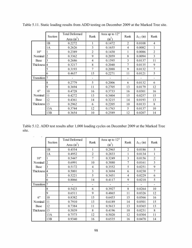
98
Table 5.11. Static loading results from ADD testing on December 2009 at the Marked Tree site.
Table 5.12. ADD test results after 1,000 loading cycles on December 2009 at the Marked Tree site.
1B 0.2272 1 0.1472 2 0.0108 41A 0.2626 3 0.1655 4 0.0082 11 0.2389 2 0.1430 1 0.0086 22 0.3362 9 0.2059 8 0.0094 33 0.2686 4 0.1595 3 0.0137 114 0.3217 8 0.2040 7 0.0135 95 0.3193 7 0.2088 9 0.0132 76 0.4637 15 0.2271 11 0.0121 5
Transition 7 - - - - - -
8 0.2779 5 0.2006 6 0.0132 69 0.3694 11 0.2705 13 0.0179 1210 0.4728 16 0.3733 16 0.0301 1611 0.4272 13 0.3404 15 0.0257 1512 0.4361 14 0.3215 14 0.0193 1313 0.2962 6 0.2205 10 0.0133 813A 0.3744 12 0.1763 5 0.0137 1013B 0.3654 10 0.2589 12 0.0207 14
Section
10" Nominal
Base Thickness
6" Nominal
Base Thickness
Total Deformed
Area (in2)Rank
Area up to 12"
(in2)Rank RankΔ12 (in)
, y
1B 0.4554 1 0.2965 2 0.0186 51A 0.4952 2 0.2833 1 0.0134 11 0.5447 7 0.3249 3 0.0156 22 0.6991 10 0.3880 7 0.0161 33 0.5172 4 0.3552 5 0.0251 94 0.5001 3 0.3694 6 0.0230 75 0.5221 5 0.3451 4 0.0229 66 0.8066 14 0.4117 9 0.0218 5
Transition 7 - - - - - -8 0.5423 6 0.3927 8 0.0264 109 0.6511 9 0.4865 11 0.0326 1210 0.8382 15 0.6453 15 0.0566 1611 0.7910 13 0.6189 14 0.0501 1512 0.7384 11 0.5613 13 0.0365 1313 0.5839 8 0.4196 10 0.0231 813A 0.7573 12 0.5020 12 0.0304 1113B 0.9340 16 0.6535 16 0.0478 14
10" Nominal
Base Thickness
6" Nominal
Base Thickness
RankArea up to 12"
(in2)Rank Δ12 (in) RankSection
Total Deformed
Area (in2)

99
Table 5.13. ADD test results after 10,000 loading cycles on December 2009 at the Marked Tree site.
Table 5.14. ADD test results after 30,000 loading cycles on December 2009 at the Marked Tree site.
, y
1B 0.5301 1 0.3545 1 0.0223 41A 0.7035 5 0.3568 2 0.0156 11 0.7206 6 0.3891 3 0.0183 22 0.8230 12 0.4525 7 0.0192 33 0.5916 2 0.4130 4 0.0299 94 0.7451 7 0.4789 9 0.0278 85 0.6014 3 0.4252 5 0.0272 66 0.8692 13 0.4469 6 0.0245 5
Transition 7 - - - - - -8 0.6957 4 0.4621 8 0.0314 109 0.7941 8 0.5621 12 0.0392 1210 1.0105 15 0.7679 16 0.0681 1611 0.9601 14 0.7419 15 0.0611 1512 0.8172 11 0.6203 13 0.0428 1313 0.8085 10 0.5023 10 0.0274 713A 0.8001 9 0.5469 11 0.0350 1113B 1.0380 16 0.7203 14 0.0551 14
6" Nominal
Base Thickness
Area up to 12"
(in2)Rank Δ12 (in) Rank
10" Nominal
Base Thickness
SectionTotal Deformed
Area (in2)Rank
1B 0.5911 1 0.3901 1 0.0259 41A 0.7565 4 0.3939 2 0.0179 11 0.7350 3 0.4061 3 0.0202 22 0.9495 12 0.5105 7 0.0221 33 0.7565 5 0.4972 6 0.0340 94 0.8014 6 0.5328 9 0.0317 75 0.6299 2 0.4392 4 0.0306 66 0.8597 9 0.4671 5 0.0268 5
Transition 7 - - - - - -8 0.8039 7 0.5275 8 0.0360 109 0.9077 11 0.6257 12 0.0441 1210 1.1126 15 0.8648 16 0.0777 1611 1.0978 14 0.8414 15 0.0701 1512 0.9514 13 0.7154 13 0.0483 1313 0.8225 8 0.5353 10 0.0329 813A 0.8762 10 0.6226 11 0.0388 1113B 1.1509 16 0.8226 14 0.0624 14
Rank Δ12 (in) Rank
10" Nominal
Base Thickness
6" Nominal
Base Thickness
SectionTotal Deformed
Area (in2)Rank
Area up to 12"
(in2)

100
for total deformed area, deflected area up to 12 inches (30.5 cm), and Δ12 are presented in Figures
5.15, 5.16, and 5.17, respectively.
With only one exception (Section 8), both the total deformed area (Figure 5.15) and the deflected
area up to 12 inches (30.5 cm) (Figure 5.16) clearly indicate that the 10-in (25.4-cm) nominal
base sections outperform the 6-in (15.2-cm) nominal base sections in terms of surface deflections
under dynamic loading. Surprisingly, for both methods of data analysis, Section 8 ranks highest
among the 6-in (15.2-cm) sections, while Section 6 ranks lowest among the 10-in (25.4-cm)
sections despite the fact that these two sections have the same geosynthetic reinforcement (refer
to Figure 3.2). Section 8 also ranked higher than some of the 10-in (25.4-cm) nominal base
course sections in terms of PLT stiffness (refer to Figure 5.10) and rutting (refer to Figures 4.2
and 4.3). It is hypothesized that the buttressing/confining effect of the driveway that intersects
Section 8 has a positive impact on the deformation characteristics of this section. All three
methods of analysis (total deformed area, deflected area up to 12” (30.5 cm), and Δ12) indicated
the general pattern noted in the rutting data (Figures 4.2 and 4.3); that Sections 1B-9 generally
outperform the other sections. Furthermore, all three ADD data analysis methods also indicated
that Section 10 performed the worst under dynamic loading and that Sections 11 and 12 also
performed very poorly, agreeing with the average rut depth values that indicated these sections
had “failed”. However, similar to the PLT results and contrary to the rutting data, all three
methods of ADD data analysis also consistently ranked Section 1 (the unreinforced section with
10-in nominal base thickness) as the 2nd best section. Again, this is likely due to the fact that
Section 1 has the thickest summed total of asphalt and base course (refer to Figure 6.13).

101
Table 5.15. Static loading results from ADD testing on May 2011 at the Marked Tree site.
Table 5.16. ADD test results after 1,000 loading cycles on May 2011 at the Marked Tree site.
Stat c
1B 0.5925 1 0.3701 2 0.0293 21A 0.6040 2 0.3424 1 0.0255 11 0.6148 4 0.3935 3 0.0311 32 0.6064 3 0.4391 4 0.0381 43 0.6271 5 0.4783 5 0.0412 54 0.7525 8 0.5506 8 0.0457 75 0.6879 7 0.4936 6 0.0429 66 1.0810 11 0.6741 10 0.0526 9
Transition 7 - - - - - -
8 0.6734 6 0.5040 7 0.0483 89 0.9042 9 0.6547 9 0.0558 1010 3.4214 16 1.8351 16 0.0995 1511 1.1457 12 0.8622 12 0.0916 1212 1.4028 13 0.9517 13 0.0942 1313 1.4745 14 1.1027 14 0.0943 1413A 1.0537 10 0.7828 11 0.0898 1113B 1.5212 15 1.1225 15 0.1316 16
Δ12 (in) Rank
10" Nominal
Base Thickness
6" Nominal
Base Thickness
SectionTotal Deformed
Area (in2)Rank
Area up to 12"
(in2)Rank
, y
1B 3.0758 6 2.3567 6 0.2023 41A 3.3324 8 2.0472 2 0.1572 11 2.4253 1 1.9424 1 0.1919 22 2.5590 2 2.0587 3 0.2063 53 2.5754 3 2.0721 4 0.2009 34 3.1033 7 2.3941 8 0.2411 75 2.6942 4 2.1491 5 0.2311 66 3.0407 5 2.4698 9 0.2463 8
Transition 7 - - - - - -8 3.4570 9 2.3911 7 0.2772 99 3.8598 10 2.5992 10 0.3074 1010 8.3671 16 7.7965 16 0.4652 1611 5.6691 13 3.7668 14 0.4211 1412 5.6073 12 3.7050 13 0.4057 1213 6.9192 15 4.9547 15 0.4578 1513A 5.6719 14 3.5406 12 0.4088 1313B 4.9119 11 3.3286 11 0.3813 11
10" Nominal
Base Thickness
6" Nominal
Base Thickness
SectionTotal Deformed
Area (in2)Rank
Area up to 12"
(in2)Rank Δ12 (in) Rank
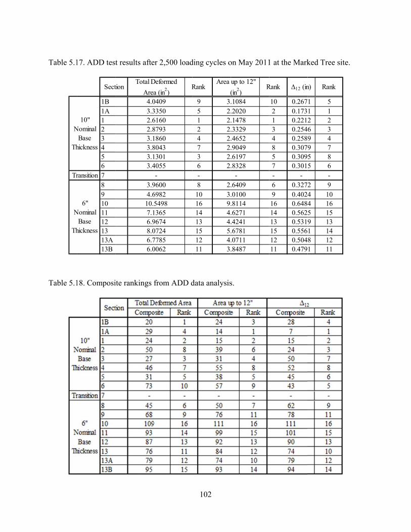
Table 5.1
Table 5.1
Tr
N
Th
N
Th
17. ADD tes
18. Composi
1B1A123456
ransition 7891011121313A13B
6" Nominal
Base hickness
10" Nominal
Base hickness
Sect
t results afte
ite rankings
4.03.32.62.83.13.83.13.4
3.94.610.7.16.98.06.76.0
tionTotal D
Area
er 2,500 load
from ADD d
04093350616087931860804313014055-
96006982549813659674072477850062
Deformed
a (in2)R
102
ding cycles o
data analysis
9 35 21 22 24 27 23 26 2-8 210 316 914 413 415 512 411 3
Area
(Rank
on May 2011
s.
.1084
.2020
.1478
.3329
.4652
.9049
.6197
.8328-
.6409
.0100
.8114
.6271
.4241
.6781
.0711
.8487
up to 12"
(in2)R
1 at the Mark
10 0.2672 0.1731 0.2213 0.2544 0.2588 0.3075 0.3097 0.301- -6 0.3279 0.40216 0.64814 0.56213 0.53115 0.55612 0.50411 0.479
Rank Δ12 (in
ked Tree site
1 51 12 26 39 49 75 85 6
-2 94 104 165 159 131 148 121 11
n) Rank
e.

103
Figure 5.15. Total deformed area composite ranking from ADD testing at Marked Tree site.
Figure 5.16. Deflected area up to 12” composite ranking from ADD testing at Marked Tree site.
1
42
8
3
7
5
10
6
9
16
1413
11 12
15
0
20
40
60
80
100
120
1B 1A 1 2 3 4 5 6 7 8 9 10 11 12 13 13A 13B
Com
pos
ite
Ran
kin
g
SectionT
rans
itio
n Se
ctio
n
3
1 2
64
8
5
97
11
16
1513
12
10
14
0
20
40
60
80
100
120
1B 1A 1 2 3 4 5 6 7 8 9 10 11 12 13 13A 13B
Com
pos
ite
Ran
kin
g
Section
Tra
nsi
tion
Sec
tion

104
Figure 5.17. Δ12 composite ranking from ADD testing at Marked Tree site.
No clear distinctions between various types of geosynthetics were observed in the ADD
results from either base course thickness, yet the ADD data and the PLT data both seem to agree
better with pavement performance than the FWD data.
5.5 Light Weight Deflectometer (LWD)
The Light Weight Deflectometer (LWD) is a portable version of an FWD, often referred
to as a Portable Falling-Weight Deflectometer (PFWD). During LWD testing, a falling weight is
raised to a desired height and allowed to fall freely onto a buffer system (refer to Figures 5.18
and 5.19). The buffer system transmits the load pulse through a loading plate that evenly
distributes the load onto the testing surface. A load cell is positioned within the LWD apparatus
to measure the impulse loads for every drop. Peak deflections are measured for every drop by a
geophone mounted inside the LWD apparatus, measuring deflections through the center of the
loading plate. An array of geophones can also be connected to the LWD to measure the
4
12
3
7 86 5
9
11
1615
13
1012
14
0
20
40
60
80
100
120
1B 1A 1 2 3 4 5 6 7 8 9 10 11 12 13 13A 13B
Com
pos
ite
Ran
kin
g
SectionT
ran
siti
on S
ecti
on

105
deflection basin caused by the impulse load. The peak deflections and impulse load are generally
displayed and recorded through a personal digital assistant (PDA) wirelessly linked to the load
cell and geophones. Deflections and loads may be either correlated directly to pavement
performance or used to determine in-situ material characteristics of the pavement layers (ASTM
E2583 – 2007).
LWD tests were conducted at the Marked Tree site during the October 2010 site visit.
The tests were first conducted on the asphalt, and then on top of the base course layers of each
test section after removing at 2-ft by 2-ft (0.61-m x 0.61-m) piece of asphalt (refer to Chapter 6).
The areas in the westbound lane adjacent to Sections 13 and 13B, referred to as 13W and 13BW,
were tested along with the 16 test sections, but tests were only performed on top of the asphalt in
these sections. All LWD tests only utilized the single geophone at the center of the loading area.
An LWD global modulus (ELWD) was calculated from these tests and ranked for all sections.
The testing procedure, data analysis method, and testing results from the October 2010
visit to the Marked Tree site are presented in the following sections.
5.5.1 LWD Testing Procedure
LWD tests were conducted at the Marked Tree site during the October 2010 site visit.
These tests were performed on the asphalt and base course surfaces of all 16 test sections, as well
as on the asphalt of the areas referred to as 13W and 13BW. The LWD device utilized was a
Dynatest 3031 Lightweight Deflectometer. A schematic of the apparatus is presented in Figure
5.18. The group used a falling mass arrangement that equaled 33 lbs (15 kg) that impacted a
buffer system consisting of four Dynatest buffer pads. LWD tests were also conducted on each
surface using a 12-in (30.5-cm) diameter loading plate and a 6-in (15.2-cm) diameter loading
plate. To alternate from the 12-in (30.5-cm) loading plate to the 6-in (15.2-cm) loading plate, the

106
snap locks must be released and the 12-in (30.5-cm) plate attachment must be rotated freely to
ensure it is disconnected from the 6-in (15.2-cm) loading plate. Unfortunately, the attachment
plate was not properly disengaged before conducting the tests with the 6-in (15.2-cm) loading
plate. Therefore, data collected using the 6-in (15.2-cm) loading plate was discarded due to
procedural error.
The LWD tests on top of the asphalt layer were conducted approximately 15 feet (4.6 m)
east of the center of each test section. The base course testing was conducted within the 2-ft x 2-
ft (0.61-m x 0.61-m) testing area once the asphalt layer was removed (excavation described in
Chapter 6). A gripped rubber mat was placed between the loading plate and the testing surface to
improve load distribution for both testing surfaces. Five falling weight sequences were
performed on the testing surfaces at each section with each size of loading plate. The load and
deflection values collected during each falling weight sequence were stored and displayed on a
PDA connected to the LWD through Bluetooth. Pictures of LWD tests being performed on the
base and asphalt are displayed in Figure 5.19.
5.6.2 LWD Data Analysis
The main unit of the LWD records the load cell and geophone data continuously
throughout the dynamic pulse from the falling weight, which is the time elapsed from the falling
weight impacting the buffer stack until the falling weight becomes stationary. Typical load-
deflection pulses for a 6-in (15.2-cm) and a 10-in (25.4-cm) nominal base thickness section on
both asphalt and base are presented in Figures 5.20 and 5.21, respectively. From the load-
deflection pulse data, the peak load and resulting peak deflection values were recorded. Note
how the peak force values remained the same while the peak deflection values were generally
greater in the 6-in sections than the 10-in sections on both asphalt and base surfaces.
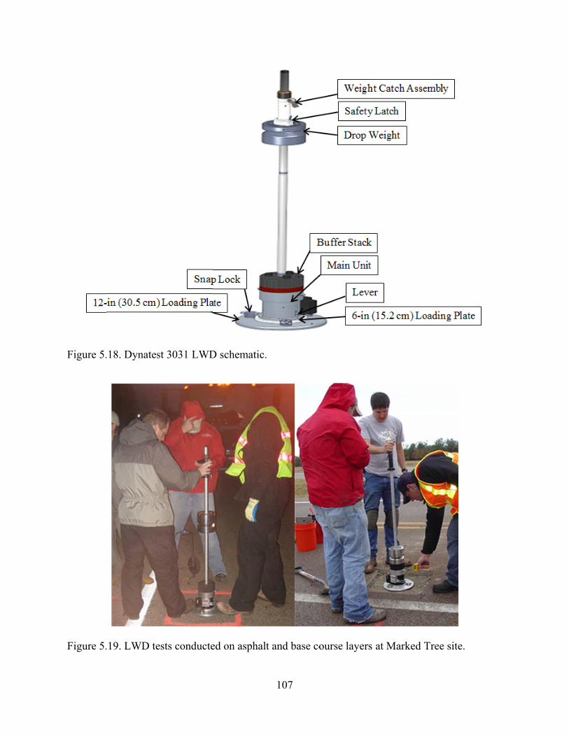
Figure 5.
Figure 5.
.18. Dynates
.19. LWD te
st 3031 LWD
ests conducte
D schematic.
ed on asphalt
107
.
t and base coourse layers at Marked T
Tree site.

108
The peak load and resulting peak deflection values are the key components in the
calculation of the LWD global modulus (ELWD). The ELWD was calculated for all sections on both
the asphalt and base surfaces. The equation for calculating the ELWD (Equation 5.5) derived by
Dynatest from Equation 8-26 in Das (1997) is as follows:
∗ ∗ ∗ (5.5)
Where: ELWD = LWD global modulus (MPa) ν = Poisson’s Ratio (0.33 for asphalt and 0.25 for base) σ = maximum applied stress (kPa) R = loading plate radius (mm) δ = maximum surface deflection (μm)
5.6.3 LWD Results
The calculated ELWD values and ranks from the 12-in (30.5-cm) loading plate on top of
both the asphalt and base layers are presented in Tables 5.19 and 5.20, respectively, and Figures
5.22 and 5.23, respectively.
The LWD rankings on the asphalt and base do not clearly reveal differences between
different types of geosynthetics in either the 10-in (25.4-cm) or 6-in (15.2-cm) base sections.
However, in general, the 10-in (25.4-cm) base sections tend to have higher global ELWD values
than the 6-in (15.2-cm) base sections, with a few exceptions. Interestingly, Section 10, which
was the lowest ranked section in terms of rutting and all other test results presented previously
(i.e., FWD, PLT and ADD), did not rank lowest (12 out of 16) based on LWD tests performed on
the asphalt surface (Figure 5.22), but did rank lowest based on LWD tests performed on the base
layers.

109
Figure 5.20. Typical load-deflection pulses from LWD testing on the asphalt surface with 12-in (30.5-cm) loading plate at the Marked Tree site on 10-in (25.4-cm) and 6-in (15.2-cm) thick base course layers.
Figure 5.21. Typical load-deflection pulses from LWD testing on the base layer with 12-in (30.5-cm) loading plate at the Marked Tree site on 10-in (25.4-cm) and 6-in (15.2-cm) thick base course layers.
-2
0
2
4
6
8
100
20
40
60
80
100
120
140
160
180
200
0 10 20 30 40 50 60 70
Forc
e (k
N)
Def
lect
ion
(μm
)
Time (ms)
Deflection (10" Base Section)
Deflection (6" Base Section)
Force (10" Base Section)
Force (6" Base Section)
LWD load-deflection pulses from testingon top of asphalt with 12-in (30.5 cm)loading plate.
-2
0
2
4
6
8
10
120
50
100
150
200
250
300
350
400
0 10 20 30 40 50 60 70
Forc
e (k
N)
Def
lect
ion
(μm
)
Time (ms)
Deflection (10" Base Section)
Deflection (6" Base Section)
Force (10" Base Section)
Force (6" Base Section)
LWD load-deflection pulses from testingon top of base layer with 12-in (30.5 cm)loading plate.

110
Table 5.19. ELWD results from LWD testing on the asphalt with 12-in (30.5-cm) diameter load plate.
Figure 5.22. ELWD results from LWD testing on the asphalt with 12-in (30.5-cm) diameter load plate
ELWD (MPa) ELWD (ksi) Rank ELWD (MPa) ELWD (ksi) Rank*
1B 237 34.44 71A 253 36.75 51 253 36.76 42 229 33.15 93 255 37.04 34 214 31.02 105 296 42.99 16 263 38.20 2
Transition 7 - - - - -8 193 27.97 119 170 24.73 1310 176 25.53 1211 168 24.34 1412 136 19.67 1613 244 35.44 6 142 20.53 1513A 234 33.95 813B 136 19.79 15 120 17.34 18
*Represents potential rank if westbound lane was used in ranking (Eastbound ranks would change accordingly).
Eastbound
10" Nominal
Base Thickness
6" Nominal
Base Thickness
SectionWestbound
75 4
9
3
10
1
2
0
11
13 1214
16
68
15
0
50
100
150
200
250
300
350
1B 1A 1 2 3 4 5 6 7 8 9 10 11 12 13 13A 13B
LW
D M
odu
lus,
EL
WD
(MP
a)
Section
Eastbound
Westbound
Tra
nsi
tion
Sec
tion

111
Table 5.20. ELWD results from LWD testing on the base with a 12-in (30.5-cm) diameter loading plate.
Figure 5.23. ELWD results from LWD testing on the base with a 12-in (30.5-cm) diameter loading plate.
ELWD (MPa) ELWD (ksi) Rank
1B 114 16.59 121A 169 24.55 31 180 26.04 22 131 19.02 83 130 18.88 94 153 22.19 45 192 27.87 16 149 21.55 5
Transition 7 - - -8 127 18.39 109 94 13.64 1510 62 8.99 1611 115 16.70 1112 98 14.28 1313 139 20.12 713A 147 21.33 613B 95 13.83 14
EastboundSection
10" Nominal
Base Thickness
6" Nominal
Base Thickness
12
32
8 9
4
1
5
0
10
15
16
11
13
76
14
0
50
100
150
200
250
1B 1A 1 2 3 4 5 6 7 8 9 10 11 12 13 13A 13B
LW
D M
odu
lus,
EL
WD
(MP
a)
Section
Tra
nsi
tion
Sec
tion

112
The LWD rankings from testing atop the base layer seem to be more similar to the
average rut depth rankings than the LWD rankings from testing atop the asphalt layer. However,
Sections 13 and 13A show much better relative performance from both forms of LWD testing
than the average rut depth values credit them with. Furthermore, while Section 8 is ranked 2 in
the average rut depth analysis, it is ranked 11 and 10 for the LWD analyses when tested atop the
asphalt and base layers, respectively. The LWD results do not seem to correlate with rutting as
well as the PLT and ADD tests.
5.6 Rolling Dynamic Deflectometer (RDD)
The rolling dynamic deflectometer (RDD) is a large truck on which a servo-hydraulic
vibrator is mounted. The vibrator is used to apply large vertical dynamic loads to rolling wheels
that come into contact with the pavement. The vibrator can apply a total vertical dynamic load up
to 33,000 lbs (147 kN). A receiver wheel located midway between the loading wheels is
primarily used to monitor the dynamic deflections. Additional rolling receivers are located at
greater distances from the applied load, enabling the measurement of dynamic deflection basins.
The truck is driven at a slow speed and continuous profiles of pavement deflection are measured
under heavy loading conditions (Bay et al. 1995). The RDD test is typically performed at
velocities of approximately 1 to 2 ft/sec (0.3 to 0.6 m/s) (Bay and Stokoe 1998). A schematic of
the RDD, with the important components pointed out, from Bay and Stokoe (1998) is displayed
in Figure 5.24.

113
Figure 5.24. Schematic of RDD with important testing features labeled (Bay and Stokoe 1998).
The University of Texas’s RDD was mobilized to the Marked Tree site for testing during
the May 2011 site visit. The testing was conducted very quickly compared to the majority of the
tests conducted at the site. The RDD was driven down the eastbound lane in the eastern
direction, referred to as the first path. The RDD was then driven down the westbound lane in the
eastern direction, completing the second path. Continuous deflection profiles were created from
the data collected during the RDD test.
5.6.1 RDD Test Procedure
The RDD test paths were in the center of the east and west bound lanes, traveling from
approximately 300 feet (91.4 m) west of Section 13B to approximately 300 feet (91.4 m) east of
Section 1B [approximately 1450 ft (442 m) total]. The static load applied during the testing was
8 kips (35.6 kN), and the dynamic load was 6 kips (26.7 kN) peak-to-peak. The loading
frequency was 30 Hz. The RDD was equipped with three sensors positioned in the center of the
114
lane. Sensor 1 was located between the loading rollers. Sensor 2 was positioned 2.5 feet (0.76 m)
in front of Sensor 1, and Sensor 2 was positioned 2 feet (0.61 m) in front of Sensor 2.
The RDD test was conducted by applying the combined loads (dynamic superimposed on
the static), and then slowly driving over the center of each lane, traveling from west to east. The
applied forces and displacements at each rolling sensor were constantly monitored during testing.
The position of the RDD was constantly calculated using a distance encoding device based on
the known starting position (Bay and Stokoe 1998). A picture of the RDD at the Marked Tree
site is displayed in Figure 5.25.
5.6.2 RDD Data Analysis
During the RDD testing, a continuous deflection profile was calculated for each path.
Raw deflection values were averaged over 1-ft (0.3-m) increments to smooth out noise. Only the
Sensor 1 deflection data is presented herein. The continuous deflection profiles in the eastbound
and westbound lanes are presented in Figure 5.26. Note that all of the highest deflections
occurred in the westbound lane, particularly across from Section 10 and Sections 12, 13 and
13A, in the areas where significant rutting leading to failure had occurred. It is also important to
point out that while the deflections in the westbound lane across from Section 13B (referred to as
Section 13BW) were low this section had recently been patched due to excessive rutting, which
resulted in lower dynamic deflections. The deflection values from the profiles within each 50-ft
(15.2-m) long section were averaged to obtain a single deflection value for each section.

Figure 5.
Figure 5.at the Ma
0
5
10
15
20
25
30
35
Def
lect
ion
(m
ils/
10k
ips)
.25. Univers
.26. RDD Searked Tree s
1B 1A
ity of Texas
ensor 1 contiite.
1 2
’s RDD at th
inuous defle
Eastboun
Westboun
3 4 5
115
he Marked T
ction profile
Sections
nd (Sensor 1)
nd (Sensor 1)
6 7 8
Tree site.
e of the eastb
9 10
bound and w
11 12 13
westbound la
13A 13B
anes

116
5.6.3 RDD Results
Only the RDD results from Sensor 1 were analyzed and ranked. Sensor 1 is located
between the rolling loading wheels. The average deflection values are presented in terms of
mils/10 kips. The results and ranks are presented in Table 5.21. Figure 5.27 is a graphical
representation of the average deflection results. The deflection values in Table 5.21 indicate that
the 10-in (25.4-cm) base sections only cover a range of 2.5 mils/10 kips, ranging from 15.4 to
17.9 mils/10 kips, while the 6-in (15.2-cm) base sections are more variable and cover a range of
7.5 mils/10 kips, ranging from 12.3 to 19.8 mils/10 kips. The RDD results do not really follow
the same trend as the rutting results (i.e., generally better performance in Sections 1B – 9 than
Sections 10 – 13B), and do not segregate the 10-in (25.4-cm) sections from the 6-in (15.2-cm)
sections as clearly as the PLT and ADD results presented previously. Many of the 6-in (15.2-cm)
sections yielded lower deflection values on average. This is perplexing because the continuous
deflection profiles clearly detected anomalies (patches in the asphalt) that were present in the
pavement. It is possible that either the static or dynamic load fluctuated slightly while driving
down the pavement. However, Section 8 (the buttressed section) is one of the better performing
sections in terms of RDD deflection, which agrees well with the average rut depth measurements
that rank Section 8 second. Section 10 performed poorly during the RDD testing (ranked 15),
which also has the worst average rut depth within the eastbound sections. Section 13B was the
poorest performing section during the RDD testing, which is somewhat consistent with the ADD
results presented herein. Yet, Section 13B does not have nearly the greatest average rut depth in
comparison to all other 6-in (15.2-cm) sections.

117
Table 5.21. Average Sensor 1 deflections from RDD testing at the Marked Tree site.
Figure 5.27. Sensor 1 average deflections from RDD testing at the Marked Tree site.
1B 17.5 111A 17.7 131 16.0 72 17.3 103 17.9 144 17.5 125 16.4 86 15.4 6
Transition 7 - - - -8 12.3 19 15.3 410 18.2 1511 16.8 912 14.3 313 13.9 2 18.5 1713A 15.4 513B 19.8 16 12.7 2
* Represents potential rank if west bound lane was included in ranking (East Bound rankings would change accordingly).
6" Nominal
Base Thickness
SectionRank
Avg. Deflection (mils/10 kips)
Rank*Avg. Deflection (mils/10 kips)
West BoundEast Bound
10" Nominal
Base Thickness
11 13
7
1014
12
8
6
1
4
15
9
32
5
16
10
12
14
16
18
20
22
1b 1a 1 2 3 4 5 6 7 8 9 10 11 12 13 13a 13b
Def
lect
ion
(mil
s/10
kip
s)
Section
East Bound
West Bound
Tra
nsi
tion
Sec
tion

118
5.7 Composite Ranking from all Deflection-Based Test Results from the Marked Tree Site
A total composite ranking from the deflection-based testing performed at the Marked
Tree site was calculated and used to rank the test sections. The composite value is the summation
of the ranks from all the data analysis methods presented in the previous sections from the
following tests: FWD, PLT, ADD, LWD, and RDD. Test-specific composite rankings were
calculated for the deflection-based tests that had multiple data analysis methods associated with
them (i.e., FWD, ADD, and LWD) prior to compiling the final composite ranking presented in
this section. The test-specific composite rankings were created to avoid weighing the results
from one test where multiple types of data analysis yielded a lot of rankings (e.g., ADD) more
heavily than another test with only a single type of analysis and ranking (e.g., RDD). The test-
specific composite values were then ranked from lowest composite value to highest composite
value, receiving new overall rankings from 1 to 16, respectively. The composite rank values and
new overall rankings are presented in Table 5.22 and are graphically represented in Figure 5.28.
Note that the rankings in Table 5.22 and Figure 5.28 can be misleading. Though Section 1B and
Section 6 are ranked 6 and 7, respectively, the difference in the composite values is exactly one,
while Sections 9 and 12 are ranked 12 and 13, respectively; the difference in the composite
values is 11.
The overall composite rankings agree with the average rut depth in the sense that Section
10 is the worst in terms of actual performance (average rut depth) and relative performance
(composite ranking from deflection-based tests). However, Section 8 is ranked 7 in the
deflection-based tests composite rankings, which is the best ranking of any 6-in (15.2-cm)
nominal base section, but Section 8 has the second least amount of average rut depth among all

119
Table 5.22. Composite ranking from all deflection-based tests conducted at the Marked Tree site.
Figure 5.28. Composite ranking from all deflection-based testing at the Marked Tree site.
1B 35 61A 23 21 14 12 36 73 32 54 42 105 26 36 26 3
Transition 7 - -8 36 79 49 1210 76 1611 64 1412 60 1313 39 913A 46 1113B 71 15
Note: composite values are composed of thesummation of rankings from FWD, PLT, ADD,LWD, and RDD testing.
Section Composite Rank
10" Nominal
Base Thickness
6" Nominal
Base Thickness
6
2
1
75
10
3 3
0
7
12
16
1413
9
11
15
0
10
20
30
40
50
60
70
80
90
1B 1A 1 2 3 4 5 6 7 8 9 10 11 12 13 13A 13B
Com
pos
ite
Ran
k
Section
Tra
nsi
tion
Sec
tion

120
sections (refer to Figure 4.3). Additionally, Section 1 is ranked first in overall deflection-based
tests, yet ranked worst among the 10-in (25.4-cm) nominal base course sections in terms of
rutting. Obviously, the overall deflection-based composite rankings do not match exactly with
the average rut depth rankings, but the composite deflection-based rankings somewhat agree
with the general rutting trend of better performance in Sections 1B – 9 and poorer performance
in Sections 10 – 13B. Furthermore, the overall deflection-based results also rank Sections 10, 11
and 12 (the three sections in the eastbound lane that had “failed” in terms of rutting) as three out
of the top four poorest sections, excluding the two westbound areas (13W and 13BW) which
were not tested during most of the deflection-based testing. It seems clear, based on rutting and
the overall deflection-based results that the nominal base thicknesses [(10-inches (25.4-cm)
versus 6-inches (15.2-cm)] significantly influences relative pavement performance and
overwhelms subtle differences in geosynthetic type (or even no reinforcement) within any give
base course thickness.
5.8 Composite Ranking from PLT and ADD Test Results from Marked Tree Site
It is clear from comparing the rankings for the individual deflection-based tests that the
PLT and ADD tests yielded results that more closely correlated to rut depth than the other three
deflection-based tests (FWD, LWD, and RDD). To determine if the combined results from these
two deflection-based tests (PLT and ADD) could more closely approximate pavement
performance than the composite of all five deflection-based tests (refer to Figure 5.28) the
research group decided to develop a composite ranking only based on the final rankings for the
PLT and ADD tests. These composite values are tabulated in Table 5.23 and graphically
presented in Figure 5.29.

121
Table 5.23. Composite ranking from PLT and ADD tests conducted at the Marked Tree site.
Figure 5.29. Composite ranking from PLT and ADD testing at the Marked Tree site.
1B 6 31A 3 11 3 12 11 53 8 44 16 85 14 76 16 8
Transition 7 - -8 13 69 20 1010 32 1611 30 1512 27 1413 23 1113A 24 1213B 26 13
Note: composite values are composed of thesummation of rankings from PLT and ADD testing.
Section Composite Rank
10" Nominal
Base Thickness
6" Nominal
Base Thickness
3
1 1
5
4
87
8
0
6
10
1615
14
1112
13
0
5
10
15
20
25
30
35
1B 1A 1 2 3 4 5 6 7 8 9 10 11 12 13 13A 13B
Com
pos
ite
Ran
k
Section
Tra
nsi
tion
Sec
tion

122
In comparison with the average rut depth rankings presented in Figure 4.3, it is clear that
the composite rank of the PLT and ADD rankings has the same general rutting trend of better
performance in Sections 1B – 9 and poorer performance in Sections 10 – 13B. Furthermore, the
overall deflection-based results also rank Sections 10, 11 and 12 (the three sections in the
eastbound lane that had “failed” in terms of rutting) as the three worst sections in terms of
deflection-based results from PLT and ADD. Additionally, Section 8 was the best 6-in (15.2-cm)
nominal base section in terms of both deflection-based results from PLT/ADD and rutting
measurements. However, the deflection-based results from PLT and ADD still indicate that
Section 1 (unreinforced) is one of the best sections overall despite being the worst 10-in (25.4-
cm) nominal section in terms of rutting. The combined PLT and ADD results are a slight
improvement over the composite results from all deflection-based tests, but still do not match the
rutting measurements exactly.
Again, no clear pattern exists in the combined PLT and ADD data that would suggest a
difference in performance base on geosynthetic type, or even a favorable difference between
reinforced and unreinforced sections within a given nominal base course thickness.
5.8 Conclusions from Deflection-Based Test Results
Results from PLT and ADD deflection-based tests (Figure 5.29) clearly identified
Sections 10, 11 and 12 as the worst sections in the eastbound lane (note that deflection-based
tests were generally not conducted in Sections 13W and 13BW in the westbound lane). These
sections were also the same sections that had “failed” based on rutting measurements (Figures4.2
and 4.3). Therefore, one may conclude that these tests were successful at inferring relative
pavement performance in terms of identifying sections that had, or were about to, rut to the point

123
of “failure”. Furthermore, the PLT and ADD deflection-based tests also clearly indicated the
general rutting trend of better performance in Sections 1B – 9 and poorer performance in
Sections 10 – 13B. However, beyond successfully identifying failed sections and showing
general agreement in rutting trends, the deflection-based tests did not perfectly correlate with the
more subtle differences in pavement performance as quantified by average rut depth values. For
example, Section 1 (unreinforced) has the highest combined PLT and ADD deflection-based
composite ranking, yet Section 1 has the greatest average rut depth among the 10-in (25.4-cm)
base sections. Still, the average April 2011 rut depth difference between the best ranked section
(Section 6) and the 11th ranked section (Section 1) is only approximately 0.19 in (0.48 cm) and
due to the method for collecting the average rut depth values they can only be considered
accurate within approximately +/- 0.125 in (0.318 cm).
Trends indicating benefits from the addition of geosynthetics are hard to observe in either
the rutting measurements or results from the deflection-based tests. Among the deflection-based
tests analyzed herein, the PLT and ADD test agreed best with the average rut depth values and
these tests should be further studied to determine if they can detect more subtle differences in
relative pavement performance. Some sort of data normalization based on absolute base course
thickness or pavement stiffness may be required to detect these subtle differences. No doubt
others will seek to analyze and interpret this data in a different manner in the future.

124
Chapter 6
6.0 Forensic Excavation and Subsurface Layer Properties
6.1 Overview
In the Spring of 2010, AHTD personnel noticed that some of the sections of Frontage
Road 3, especially in the westbound lane, were failing or nearing failure. In a few locations, rut
depths exceeded several inches (refer to Figure 6.1). The research group was faced with
answering the question of what factor, or combination of factors, was responsible for failure in
certain sections and not others. So, it was decided that a forensic excavation needed to be
conducted in each of the test sections in the eastbound lane, as well as a couple of areas in the
westbound lanes opposite Sections 13 and 13B (referred to as Sections 13W and 13BW) where
significant rutting was observed.
The forensic excavation was conducted during the October 2010 site visit. Additional in-
situ test were conducted and samples were gathered in all sections for laboratory testing. These
samples included bagged samples, bulk samples, and Shelby tube samples. The process of the
forensic excavation, as well as the layer and soil properties determined through the forensic
excavation, are discussed in this chapter. A composite rank of the soil and layer properties
deemed to be influencing failure is calculated and compared to the average rut depth values
presented in Chapter 4 (refer to Table 4.4 and Figure 4.6) to determine why failure occurred in
certain sections and not others.
6.2 Introduction
Prior to the October 2010 Marked Tree site visit, the research group decided to conduct
tests on top of the asphalt layer, the base layer, and the subgrade layer in a 2-ft x 2-ft (0.61-m x

Figure 6.
0.61-m)
section. T
layers, re
asphalt, L
each sec
dynamic
conducte
inch (5.1
removal
for testin
removing
.1. Rut depth
square testi
To conduct
espectively,
LWD tests w
tion. After r
cone penet
ed on the bas
-cm) increm
of the base
ng of in-situ
g the base l
h exceeding
ing area in
tests on top
had to be re
were conduc
removing th
trometer (D
se layer in e
ments by adv
layers, bag a
u moisture c
layers and m
3 inches (7.6
the outside
p of the base
emoved sequ
cted on the
he asphalt a
DCP), and in
each section.
vancing the n
and bucket b
content and
measuring th
125
6 cm) in Sec
(right) whe
e layer and t
uentially fro
2-ft x 2-ft (
nd measurin
n-situ Calif
. Nuclear de
nuclear gage
bulk sample
base layer
heir thickne
ction 13BW
eel path 8-ft
the subgrade
om each sec
(0.61-m x 0.
ng its thickn
fornia Beari
ensity gage r
e probe throu
es were obta
gradation a
ess, nuclear
during May
ft east of th
e layer, the
ction. Prior t
.61-m) squar
ness, LWD,
ing Ratio (C
readings wer
ugh the base
ained every 2
s a function
density gag
y 2010.
he center of
asphalt and
to removal o
re testing ar
nuclear den
CBR) tests
re collected
material. D
2 inches (5.1
n of depth.
ge readings
each
d base
of the
rea in
nsity,
were
in 2-
During
1 cm)
After
were

126
collected in 2-inch (5.1 cm) increments through the top 12 inches (30.5 cm) of the subgrade.
Then, in-situ CBR tests were conducted on the subgrade layer and undisturbed (Shelby tube)
samples were pushed in the northeast and southwest corners of the testing area. Additionally, bag
samples for in-situ moisture content and plasticity index were collected every 2 inches (5.1 cm)
of subgrade down to 6 inches (15.2 cm).
The in-situ DCP and CBR tests conducted on the base and subgrade layers were used to
determine the relative stiffness of the two layers in each section. Additionally, resilient modulus
(Mr) and unconsolidated undrained (UU) triaxial tests were conducted on the Shelby tube
samples collected in the subgrade to evaluate the stiffness/strength properties of the subgrade
soils. The excavation, sampling, and testing procedures previously discussed will be described in
greater detail, along with the results, in the following sections.
6.3 Forensic Excavation
On the October 2010 Marked Tree site visit, the research group conducted a forensic
excavation in each test section, including 13W and 13BW. The forensic excavation was
conducted so the research group could perform in-situ tests on, and collect samples of, the base
layer and subgrade layer to attempt to determine why certain sections were performing more
poorly than others. The forensic excavation was conducted in the following sequence for each
test section:
1. The locations for the 2-ft x 2-ft (0.61-m x 0.61-m) excavation and testing locations were marked 15 feet (4.6 m) east of the sensor locations in each section on the outside wheel path (Figure 6.2).
2. LWD tests were conducted on the asphalt layer using a 12-in (30.5-cm) diameter plate and a 6-in (15.2-cm) diameter plate. (refer to Section 5.5 and Figure 5.19).
3. The perimeter of the 2-ft x 2-ft (0.61-m x 0.61-m) layer of asphalt was carefully cut using a concrete saw (Figure 6.3a) and the asphalt layer was removed with a pry-bar

Figure 6.
4
5
6
7
8
9
1
.2. Excavatio
(Figure 6situ moist
. Asphalt lcenter of t
. Nuclear devery 2 inarea (Figu
. DCP testsinches (12
. LWD testand a 6-in
. In-situ CB
. In-situ mobase cour
0. The base 1 and 13geosyntheout of the
on and testin
.3b). No watture content
layer thicknthe excavati
density gaugnches (5.1 cure 6.4a).
s were cond20 cm)] in th
ts were condn (15.2-cm) d
BR tests wer
oisture conterse (Figure 6
course was c3 (Figure 6.etic interface test area an
ng area at Se
ter was useddata for the
ness measureon area usin
ge readings wcm) through
ducted throuhe southeast
ducted on thdiameter pla
re conducted
ent and bulk.7).
completely e8), and thee for all othe
nd stored in b
127
ction 9 durin
d during the base and sub
ements wereng a small sc
were collectthe base in
ugh the base corner of th
he base layerate (refer to F
d on the base
k samples w
excavated tobase was
er sections (bags for testi
ng October 2
asphalt cuttbgrade.
e conductedale and a me
ted by continn the northw
and well inhe excavation
r using a 12Figure 5.19)
e layer (Figu
were collecte
o the subgradcompletely (Figure 6.9)ing discussed
2010 Marked
ting to ensur
d at each coetal rut bar.
nuously advwest corner o
nto the subgn area (Figur
2-in (30.5-cm.
ure 6.6a).
d every 2 in
de-base interexcavated t
. The geosyd in Boga (2
d Tree site v
re accuracy o
orner and in
vancing the pof the excav
grade [at leare 6.5).
m) diameter
nches (5.1 cm
rface for Secto the subgnthetics wer
2011).
visit.
of in-
n the
probe vation
ast 47
plate
m) of
ctions grade-re cut

Figure 6.
Figure 6.
.3. Cutting (a
.4. Nuclear d
(a)
a) and remov
(a)
density gaug
val (b) of asp
ge readings c
128
phalt layer f
conducted on
for base cour
n the base (a
(b)
rse testing an
(b)
a) and subgra
nd sampling
ade (b) layer
.
rs.

Figure 6.
Figure 6.
.5. DCP test
.6. CBR test
conducted i
(a)
s conducted
n southeast c
on base (a)
129
corner of ex
and subgrad
xcavation are
de (b) layers.
ea of Section
(b)
.
n 13W.

Figure 6.
Figure 6.
.7. Base laye
.8. Base-sub
er excavation
grade interfa
n and sampli
ace of Sectio
130
ing at Sectio
on 1 (no geo
on 2.
synthetics).

Figure 6.
1
1
1
14
1
T
as part of
.9. Subgrade
1. Base couconductedrut bar. Bthicknesse
2. Once the by continua depth of
3. In-situ CB
4. Shelby tuof 24 inchto collect
5. Bag sampevery 2 in
The soil prop
f the forensic
e-geosynthet
urse and aspd at each corBase coursees from the t
subgrade lauously advaf 12 inches (
BR tests wer
ubes [30-in (hes (60.9 cmundisturbed
ples for in-snches (5.1 cm
perties determ
c excavation
ic interface o
phalt combinrner and in the thicknessestotal thickne
ayer was reacancing the pr(15.2 cm) (F
re conducted
(76.2-cm) lom) in the nortd samples for
itu moisturem) for the fir
mined from
n are discuss
131
of Section 1
ned thickneshe center of s were infer
ess measurem
ched, nuclearobe every 2igure 6.4b).
d on the subg
ong; 3-in (7.6theast and sor lab testing
e content anrst 6 inches (
the in-situ
ed in the fol
A (Mirafi ge
ss (total thithe section urred from s
ments.
ar density ga2 inches (5.1
grade layer (
6-cm) diameouthwest cor(Figure 6.10
nd plasticity (15.2 cm) of
testing and
llowing secti
eogrid).
ickness) meusing a steelsubtracting t
auge reading cm) through
(Figure 6.6b)
eter] were prners of each0).
index testinf subgrade.
laboratory t
ions.
asurements l tape and a mthe asphalt
gs were collh the subgra
).
pushed to a dh excavation
ng were coll
testing condu
were metal layer
lected ade to
depth n area
lected
ucted

Figure 6.
6.4 Laye
P
of the cu
test sect
approxim
provided
Chapter
plasticity
excavatio
6.4.1 Lay
T
x 2-ft (0.
.10. Shelby t
er Propertie
rior to visiti
urrent subgra
tions, surve
mate thickne
d on the con
3).This sect
y index inf
on.
yer Thickne
The layer thic
.61-m x 0.61
tube pushed
es
ing the Mark
ade and base
ey data pre
esses of the
nstructed de
tion presents
formation g
esses
cknesses we
1-m) square
in southwes
ked Tree site
e properties
esented in
e asphalt an
ensity and m
s the layer t
athered in
ere calculated
testing area
132
st corner of e
e on October
within each
Howard (2
nd base lay
moisture con
thickness, in
each sectio
d as the diff
a. For examp
excavation a
r 2010, the r
h test section
2006) was
yers. Howev
ntent of the
n-situ moistu
on during
ferent layers
ple, once the
area.
research gro
n. During co
collected to
ver, there w
e base or su
ure content,
the Octobe
were extrac
e asphalt lay
oup was unce
onstruction o
o document
was limited
ubgrade (ref
dry density
er 2010 for
cted from th
yer was remo
ertain
of the
t the
data
fer to
y, and
rensic
e 2-ft
oved,

133
there were five thickness measurements collected: one in the center and one at each of the four
corners. To ensure continuity in the thickness measurements between layers, a flat metal bar was
placed across the test area, and thicknesses were measured relative to the nearest edge of the bar.
The bar used for measuring thicknesses was the same bar used for measuring rut depths and is
referred to herein as a “rut bar”.
The five asphalt thickness values were averaged together to obtain one comparable value
for each section. These thickness values were also obtained for the areas adjacent to Sections 13
and 13B in the west bound lane, referred to as 13W and 13BW. The same procedure was used to
obtain the average base course thickness in each section. The averaged values and rankings
assigned to each section are presented in Table 6.1 and Figures 6.11, 6.12, and 6.13. Figure 6.11
is a plot of the asphalt thicknesses, Figure 6.12 is a plot of the base thicknesses, and Figure 6.13
is a plot of the total asphalt plus base thickness. The rankings for each section are located over
the bar for each section, excluding the west bound lane sections, which were not included in the
overall rankings since these sections had not previously been a focus of testing at the site.
However, the reader is reminded that these sections (13W and 13BW) were added to the forensic
excavation because failure (major rutting) had occurred in them.
The asphalt thicknesses at the site vary from 2.0 – 2.65 inches (5.1 – 6.7 cm). There is no
clear pattern for changes in asphalt thickness in the 10-in (25.4-cm) nominal base course
sections, but the asphalt thickness tends to increase from Section 8 to Section 13B in the 6-in
(15.2-cm) nominal base course sections.
The base course thicknesses in the 10-in (25.4-cm) nominal sections vary from 8.9 – 11.3
inches (22.6 – 28.7 cm), with Section 4 and Section 1 (unreinforced) having the least and
greatest base thicknesses, respectively. Furthermore, the total base plus asphalt thicknesses in the

134
Table 6.1. Layer thicknesses collected during October 2010 site visit.
Figure 6.11. Asphalt thicknesses collected during October 2010 site visit.
Section Asphalt Base Total Asphalt Base Total
1b 2.30 9.33 11.63 7 1a 2.24 9.64 11.88 5 1 2.08 11.33 13.40 1 2 2.23 9.95 12.17 3 3 2.39 9.64 12.03 4 4 2.08 8.90 10.98 8 5 2.46 10.14 12.60 2 6 2.13 9.70 11.83 6 7 - - - - - - - -8 2.00 7.18 9.18 9 9 2.15 6.50 8.65 12 10 2.23 5.60 7.83 16 11 2.15 6.48 8.63 13 12 2.31 5.76 8.08 15 13 2.38 6.55 8.93 10 2.21 5.67 7.88 1613a 2.55 6.13 8.68 11 13b 2.65 5.45 8.10 14 1.92 5.33 7.25 18
Note: Rank was decided by Total Thickness; Total Thickness is the sum of asphalt and base thicknesses.* Represents potential rank if west bound lane was included in ranking (East Bound rankings would change accordingly).
10" Nominal
Base Thickness
6" Nominal
Base Thickness
Eastbound Thicknesses (in) Westbound Thicknesses (in)Rank*Rank
78
14
9
4
14
3
13
16
119
11
65
2
1
1.5
1.7
1.9
2.1
2.3
2.5
2.7
2.9
1B 1A 1 2 3 4 5 6 7 8 9 10 11 12 13 13A 13B
Asp
hal
t T
hic
kn
ess
(in
)
Section
Eastbound
Westbound
Tra
nsi
tion
Sec
tion

135
Figure 6.12. Base thicknesses collected during October 2010 site visit.
Figure 6.13. Total asphalt and base section thicknesses collected during October 2010 site visit.
10-in (25.4-cm) nominal sections vary from 10.98 – 13.4 inches, again with Section 4 and
Section 1 (unreinforced) having the least and greatest asphalt plus base thicknesses, respectively.
75
1
35
8
24
9
11
15
12
14
1013
16
4
5
6
7
8
9
10
11
12
1b 1a 1 2 3 4 5 6 7 8 9 10 11 12 13 13a 13b
Bas
e T
hic
kn
ess
(in
)
Section
Eastbound
Westbound
Tra
nsi
tion
Sec
tion
75
1
3 4
8
2
6
912
16
13
15
1011
14
6
7
8
9
10
11
12
13
14
1B 1A 1 2 3 4 5 6 7 8 9 10 11 12 13 13A 13B
Tot
al S
ecti
on T
hic
kn
ess
(in
)
Section
Eastbound
Westbound
Tra
nsi
tion
Sec
tion

136
Coincidentally (or perhaps not), Sections 4 and 1 are also generally ranked as “worst”
and “best” among the 10-in (25.4-cm) nominal base course sections via the combined PLT and
ADD deflection-based rankings (refer to Figure 5.29). These deflection-based tests are heavily
influenced by the thickness of the pavement material over the subgrade. The base course
thicknesses in the 6-in (15.2-cm) nominal sections vary from 5.5 – 7.2 inches (14.0 – 18.3 cm),
with Section 13B and Section 8 having the least and greatest base thicknesses, respectively.
Furthermore, the total base plus asphalt thicknesses in the 6-in (15.2-cm) nominal sections vary
from 7.8 – 9.2 inches (19.9 – 23.3 cm), with Sections 10 and 8 having the least and greatest
asphalt plus base thicknesses, respectively. Coincidentally (or perhaps not), Sections 10 and 8 are
also generally ranked as “worst” and “best” among the 6-in nominal base course sections via the
combined PLT and ADD deflection-based rankings. Furthermore, all of the sections that have
“failed” (Sections 10, 11, 12, 13W and 13BW) according to the rutting data [> 0.5 in (1.3 cm) of
rutting] also have the lowest combined asphalt and base course thicknesses (approximately 8
inches or less; refer to Figure 6.13). This cannot be coincidental. It should also be noted here that
a very clear interface existed between the base and subgrade during excavation of the
unreinforced sections (i.e., Sections 1 and 13), and that no significant loss of base course into the
subgrade or migration of fines into the base course was observed. Migration of fines into the
subgrade was studied in depth by Boga (2011).
6.4.2 Moisture Content
Moisture content of the base and subgrade layers plays a significant role in the
performance of any pavement. Furthermore, it is important to investigate the role that different
geosynthetic reinforcements play in how moisture moves throughout the pavement structure.
During the October 2010 visit, the ground on the shoulder and ditch line south of the roadway
137
was very dry, creating desiccation cracks several feet deep (Figure 6.14). Despite the fact that the
surrounding ground was extremely dry, pooling/slowly flowing water was found on top of the
subgrade in certain sections. An example of this is shown in Figure 6.15 for Section 13W. Water
appeared to be flowing through the slit-film geotextile along the interface between the base and
the subgrade. During construction this slit-film geotextile was placed along the entire westbound
lane and overlapped significantly into the eastbound lane (refer to Chapter 3). It did not appear
that any of the geotextiles in the road were “daylighted”. Meaning, water that infiltrated the
pavement anywhere along the road was likely flowing through the geotextiles and pooling at low
spots on top of the CH subgrade instead of draining out the edges of the pavement. Furthermore,
while the ground was extremely dry in October 2010, the ditch on the south side of the road was
filled with water on many site visits (refer to Figure 6.16). During particularly wet seasons, water
would pool in the ditches all along the test sections, but would linger longer in the ditch south of
the 6-in (15.2-cm) nominal sections.
In-situ moisture content samples were collected and weighed wet in the field for
gravimetric moisture content measurements during the forensic excavation. These samples were
collected every 2 inches (5.1 cm) throughout the base layer and every 2 inches (5.1 cm) for the
first 6 inches (15.2 cm) of the subgrade. The moisture content values for these samples were
determined at the University of Arkansas lab in accordance with ASTM D2216-09. While
moisture content values were collected every 2 inches, all of the base moisture contents and all
of the subgrade moisture contents have been averaged herein to obtain a single gravimetric
moisture content for the base and subgrade in each section. The in-situ moisture content values
of the base and subgrade are presented in Tables 6.2 and 6.3, respectively. The in-situ moisture

Figure 6.
Figure 6.
.14. Desiccat
.15. Pooling
tion cracks i
water on su
in ground so
ubgrade of Se
138
outh of test si
ection 13W i
ite in Octobe
in October 2
er 2010.
2010.

Figure 6.
Table 6
.16. Standing
.2. Average
Tran
* Re (Eas
6" NB
Thi
NoB
Thi
g water south
in-situ gravi
1B1A123456
nsition 7891011121313A13B
epresents potenst Bound rank
Nominal Base ickness
Sect
10" ominal Base ickness
h of Section
imetric base
3.823.492.773.543.433.042.552.92
-2.633.303.282.763.233.002.853.16
ntial rank if weings would cha
tionWat
Content
Ea
139
ns 8 through
e moisture co
2 169 147 44 153 134 85 12 6
-3 20 128 116 33 100 75 56 9est bound lane ange according
ter t (%)
Rank
ast Bound
13B in May
ontents from
-
4.57
3.66was included
gly).
kWater
Content (%
Wes
y 2011.
m the October
-
18
16in ranking
%)Rank*
st Bound
r 2010 site v
visit.

140
Figure 6.17. Average in-situ base gravimetric moisture contents from samples collected in October 2010.
Table 6.3. Average in-situ gravimetric subgrade moisture contents from the October 2010 site visit.
1614
4
15 13
8
1
6
0
2
12 11
3
107
59
0.0
0.5
1.0
1.5
2.0
2.5
3.0
3.5
4.0
4.5
5.0
1B 1A 1 2 3 4 5 6 7 8 9 10 11 12 13 13A 13B
Bas
e M
oist
ure
Con
tent
(%
)
Section
East Bound
West Bound
Tra
nsi
tion
Sec
tion
1B 15.47 11A 16.69 31 16.33 22 20.46 73 21.19 84 22.96 105 23.24 116 23.88 14
Transition 7 - - - -8 23.47 139 21.19 910 23.35 1211 23.95 1512 19.13 513 32.24 16 26.97 1713A 17.43 413B 20.43 6 22.47 10
* Represents potential rank if west bound lane was included in ranking (East Bound rankings would change accordingly).
6" Nominal Base
Thickness
SectionWater
Content (%)Rank
10" Nominal
Base Thickness
Water Content (%)
Rank*
East Bound West Bound

141
Figure 6.18. Average in-situ gravimetric subgrade moisture contents from samples collected in October 2010.
content values and ranks for the base and subgrade layers are also graphically displayed in
Figures 6.17 and 6.18, respectively.
The average base moisture content values only range from approximately 2.6% - 3.8%,
which are much lower than the optimum moisture content range of 6.5% - 8.2% reported in
Howard (2006) (refer to Table 3.4). Therefore, on average, the base would be considered quite
dry at the time of the forensic excavation with no significant differences between sections.
According to Howard (2006), the optimum moisture content (OMC) of the compacted subgrade
was 16.8% (refer to Chapter 3, Section 3.3.1). Note, from the in-situ moisture content data
collected during October of 2010, only Sections 1B, 1A, 1, and 13A are within ± 2% of OMC.
The average moisture contents from Sections 2 through 13B, excluding 13A, are wet of optimum
and range from approximately 19.1% - 32.2%. However, the majority of the sections have a
subgrade moisture content between 20% - 25%. Recalling that Sections 10, 12, 13W and 13BW
had “failed” according to rutting, there does not appear to be a strong direct correlation between
13 2
7 810 11 14
0
139
12 15
5
16
4
6
0
5
10
15
20
25
30
35
1B 1A 1 2 3 4 5 6 7 8 9 10 11 12 13 13A 13B
Subg
rade
Moi
stur
e C
onte
nt (
%)
Section
East Bound
West Bound
OMC = 16.8%
Tra
nsi
tion
Sec
tion
142
subgrade in-situ moisture content and the pavement performance, especially considering that
Section 13 had the highest subgrade moisture content and had not “failed” and Section 12 had
the fifth lowest moisture content and had “failed”. However, there could be a hidden, indirect
link between the pavement performance and the combined effects of total section thickness and
subgrade moisture content.
6.4.3 Plasticity Index
During the forensic excavation in October 2010, bag samples of the subgrade were
collected every 2 inches (5.1 cm) down to a depth of 6 inches (15.2 cm) for plasticity index (PI)
testing. The plasticity index testing was conducted per ASTM D4318 as documented in Boga
(2011). The bag samples were oven dried then ground up and passed through a No. 40 sieve until
enough material was obtained to conduct the liquid limit (LL) and plastic limit (PL) tests.
The plasticity index (PI) is the range of water content over which a soil behaves
plastically, or the difference between the LL and the PL. PI values were calculated for three 2-in
(5.1-cm) layers in the top 6 inches (15.2 cm) of subgrade soil by Boga (2011). These values were
then averaged herein to obtain one overall PI value for each section. The average PI values and
the associated rankings are presented in Table 6.4. The lowest PI value has the best ranking and
so on. The PI values and ranks are graphically displayed in Figure 6.19.
The plasticity index values range from approximately 13 (Section 1A) to 41 (Section 13).
Despite being unreinforced, with the highest average in-situ subgrade water content and the
highest average subgrade PI, Section 13 is not one of the sections that has “failed” according to
rutting data (refer to Figures 4.2 and 4.3). Furthermore, Section 12, which has “failed”, has the
second lowest PI. It does not appear that the subgrade PI values have a direct correlation to the
pavement performance for the current data set.

143
Table 6.4. Average plasticity index (PI) values of subgrade soils at Marked Tree site.
Figure 6.19. Average plasticity index (PI) values of subgrade soils at Marked Tree test site.
Section LL PL PI Rank LL PL PI Rank*
1B 36 17 19 31A 29 16 13 11 36 15 21 42 39 18 21 43 45 19 26 74 49 19 30 135 48 19 29 116 55 23 32 14
Transition 7 - - - - - - - -8 53 26 27 89 46 18 28 910 49 21 28 911 51 22 29 1112 32 14 18 213 66 25 41 16 60 19 41 1713A 62 22 40 1513B 40 16 24 6 47 19 28 11
* Represents potential rank if west bound lane was included in ranking (East Bound rankings would change accordingly).
10" Nominal
Base Thickness
6" Nominal Base
Thickness
East Bound West Bound
3
1
4 4
7
13 1114
0
8 9 9 11
2
16 15
6
0
5
10
15
20
25
30
35
40
45
1B 1A 1 2 3 4 5 6 7 8 9 10 11 12 13 13A 13B
Pla
stic
ity
Ind
ex
Section
East Bound
West Bound
Tra
nsi
tion
Sec
tion

144
6.4.4 Dry Density
Estimates of in-situ dry density were calculated using two methods. The first method was
based on nuclear density gage readings in each layer collected at 2-inch (5-cm) increments
throughout the base and the first 6 inches (15.2 cm) of the subgrade. The total density values
collected from the nuclear density gauge were used to calculate dry density using the gravimetric
moisture contents discussed in Section 6.4.2. Meaning, the estimates of moisture content from
the nuclear density gage were not used to calculate dry density because the gravimetric moisture
contents were believed to be more accurate. Average dry densities for the base and subgrade
calculated using total density values from the nuclear density gage and gravimetric water
contents are provided in Table 6.5. The base dry density values are plotted in Figure 6.20 and
range from 136.4 to 149.7 pcf (2265 – 2398 kg/m3). The range of maximum base dry densities
from modified proctor tests presented in Howard (2006) is approximately 142.2 to 144.0 pcf
(2278 – 2307 kg/m3), and the constructed dry densities measured with a nuclear gauge ranged
from approximately 148.5 to 150.3 pcf (2379 – 2408 kg/m3), which were believe to be too high
(refer to Table 3.4). The base dry density values are randomly varying amongst the sections, yet
the average variation of base dry density between sections is approximately 3.2 pcf (51.3 kg/m3).
Note that of the sections that have “failed” (Section 10, 11, 12, 13W and 13BW) , only
Section 13BW has a substantially lower in-situ base dry density [136.4 pcf (2185 kg/m3)], which
is only 6 pcf (96 kg/m3) below the maximum dry density and still within 95% of modified
proctor. Furthermore, Section 11 has the highest in-situ base dry density. Again, for this data set
it does not appear that differences in the dry density of the base are closely correlated to
pavement performance.

145
Table 6.5. Average in-situ dry density values of base and subgrade at the Marked Tree site obtained from nuclear gage total density and gravimetric water content.
Figure 6.20. Base in-situ dry densities calculated from October 2010 site visit.
1B 147.1 10 112.6 11A 143.2 14 104.6 31 149.4 4 105.4 22 141.4 16 98.5 153 143.0 15 103.2 64 147.2 9 99.1 125 149.4 3 101.2 86 148.8 5 98.7 13
Transition 7 - - - - - - - -8 149.5 2 100.0 109 146.0 12 103.5 410 148.4 6 98.7 1411 149.7 1 99.3 1112 146.6 11 102.0 713 147.6 8 96.2 16 147.2 10 92.4 1813A 144.4 13 103.4 513B 147.9 7 100.8 9 136.4 18 98.8 13
* Represents potential rank if west bound lane was included in ranking (East Bound rankings would change accordingly).Avg. dry density values were determined from total density readings from nuclear density gauge and in-situ moisture content.
6" Nominal
Base Thickness
Avg. Dry Density (pcf)
Rank
10" Nominal
Base Thickness
East BoundBase Subgrade
Avg. Dry Density (pcf)
RankSection Rank*
West BoundBase Subgrade
Avg. Dry Density (pcf)
Rank*Avg. Dry
Density (pcf)
10
14
4
1615
9
35 2
12
61
118
13
7
130
135
140
145
150
155
160
1B 1A 1 2 3 4 5 6 7 8 9 10 11 12 13 13A 13B
Dry
Den
sity
(p
cf)
Section
East Bound
West Bound
Tra
nsi
tion
Sec
tion

146
The other method only allows for the calculation of the subgrade dry density. This
method utilized the Shelby tube samples from both resilient modulus (Mr) testing and
unconsolidated undrained (UU) triaxial testing of intact subgrade specimens. A total density
value was calculated for each Shelby tube sample. The height and diameter were calculated by
averaging three measurements of each, for each sample, to use for the volume calculations. Then,
the moist sample was weighed and divided by this volume, producing total density. Once the
total density and water content values were calculated for each sample, the dry density values
were easily obtained. The Shelby tube sample dry densities from Mr and UU testing are
presented in Tables 6.6 and 6.7, respectively.
The subgrade dry density values from all three estimates were averaged together to
account for variances in the multiple determination methods, as well as to have one number for
comparison to pavement performance for each section. The average dry density values of the
subgrade and the associated rankings are presented in Table 6.8 and Figure 6.21. The average
subgrade dry density values range from 94.8 to 110.2 pcf (1519 – 1765 kg/m3). The maximum
proctor dry density determined in Howard (2006) was approximately 106 pcf (1698 kg/m3). The
initial compacted subgrade in October of 2004 did not achieve maximum dry density in any
sections (refer to Figure 3.11). However, after reworking of the subgrade in June 2005 all
sections exceeded maximum dry density.
The average dry density values obtained from the October 2010 forensic excavation agree
more closely with the original dry densities from October 2004 construction. From observing
Figure 6.21, it seems that the subgrade was compacted more in Sections 1B – 3 than any of the
other sections, with dry densities ranging from approximately 105.1 to 110.2 pcf (1684 – 1765
kg/m3).

147
Table 6.6. Subgrade dry densities from resilient modulus test samples.
Table 6.7. Subgrade dry densities from UU triaxial test samples.
1B 108.0 41A 107.8 51 111.1 12 108.4 23 108.2 34 100.9 135 101.1 126 101.3 10
Transition 7 - - - -8 101.2 119 99.7 1410 104.3 711 102.7 912 105.4 613 103.4 8 91.6 1713A 91.1 1613B 94.7 15 104.3 8
* Represents potential rank if west bound lane was included in ranking (East Bound rankings would change accordingly).
10" Nominal
Base Thickness
6" Nominal
Base Thickness
RankDry Density
(pcf)Section
East BoundDry Density
(pcf)Rank*
West Bound
1B 106.7 91A 112.3 31 114.1 22 108.4 43 114.2 14 99.5 145 102.0 136 103.4 10
Transition 7 - - - -8 107.1 89 103.3 1110 103.1 1211 107.5 612 95.2 1513 84.9 16 103.4 1213A 107.8 513B 107.5 7 108.1 5
* Represents potential rank if west bound lane was included in ranking (East Bound rankings would change accordingly).
East Bound West Bound
SectionDry Density
(pcf)Rank
Dry Density (pcf)
Rank*
10" Nominal
Base Thickness
6" Nominal
Base Thickness

148
Table 6.8. Average subgrade dry densities from three determination procedures.
Figure 6.21. Average subgrade in-situ dry densities determined from three testing procedures.
1B 109.1 21A 108.2 41 110.2 12 105.1 53 108.6 34 99.8 155 101.4 106 101.1 11
Transition 7 - - - -8 102.8 79 102.1 810 102.0 911 103.2 612 100.9 1313 94.8 16 95.8 1713A 100.7 1413B 101.0 12 103.7 6
* Represents potential rank if west bound lane was included in ranking (East Bound rankings would change accordingly).
Avg. Dry Density (pcf)
RankAvg. Dry Density
(pcf)Rank*
East Bound West Bound
Section
10" Nominal
Base Thickness
6" Nominal Base
Thickness
2 41
5
3
1510 11
7 8 96
13
16
14 12
80
85
90
95
100
105
110
115
1B 1A 1 2 3 4 5 6 7 8 9 10 11 12 13 13A 13B
Dry
Den
sity
(p
cf)
Section
East Bound
West Bound
Tra
nsi
tion
Sec
tion

149
The rest of the sections, excluding Section 13, have very similar average subgrade dry
density values ranging from 99.8 to 102.8 pcf (1599 – 1647 kg/m3), which are within the range
of 94% to 97% of maximum proctor. The subgrade in Section 13 (unreinforced) has the lowest
average in-situ dry density [94.8 pcf (1519 kg/m3) or 89% of maximum proctor], highest in-situ
water content, and highest PI, yet it has not “failed”. However, the westbound lane at this exact
location (Section 13W, reinforced with a slit-film geotextile) has almost identical properties and
has “failed”. The only observable difference is that Section 13 has approximately one more inch
of combined asphalt and base than Section 13W. Again, for this data set it does not appear that
differences in the dry density of the subgrade are closely correlated to pavement performance.
6.5 Strength/Stiffness Testing
During the October 2010 forensic excavation, in-situ strength/stiffness tests were
conducted on site (DCP and CBR) and undisturbed samples were collected for laboratory testing
of the subgrade (Mr and UU). The testing procedures, data analysis methods, and results from
the strength/stiffness tests conducted on the base and subgrade soils are presented in the
following sections.
6.5.1 Dynamic Cone Penetrometer (DCP)
The Dynamic Cone Penetrometer (DCP) test is a test method that measures the
penetration rate of a cone through undisturbed soil, compacted materials, or both. The
penetration rate may be related to in-situ strength (ASTM D6951-09), as well as strata thickness
and bearing capacity. DCP is typically used in horizontal construction applications, such as
pavements and shallow foundations. Normally the DCP is used to assess material properties to a
depth of 30 inches (76.2 cm) below the surface, but with extensions, the drive rod can be
advanced to 6 feet (1.8 m). The operator drives the DCP tip into the soil by lifting the sliding

150
hammer to the handle then releasing it. The total penetration for a given number of blows is
measured and recorded in mm/blow (Kessler 2005). Hammer blows are applied to the drive rod
until a specified depth of investigation is reached.
DCP tests were conducted at the Marked Tree site on two occasions: December 2009 and
October 2010. The December 2009 DCP testing was conducted by drilling a hole through the
asphalt in each test section to the assumed top of base. During the October 2010 site visit, the
asphalt layer was removed from the base layer, so the DCP was placed directly on the base layer
to perform the testing. For both test dates, the DCP was penetrated to a depth of approximately
48 inches (1200 mm) below the asphalt surface.
6.5.1.1 DCP Testing Procedure
All DCP testing was conducted with a Kessler Model 100 Dynamic Cone Penetrometer.
A schematic of the DCP used for testing is presented in Figure 6.22. Each test was conducted
with the 17.6 lb (8 kg) hammer, causing drop energy of approximately 33 lb-ft (45 N-m) per
blow. Each test was conducted with at least two persons. One person was assigned to hold the
DCP apparatus vertical while lifting and dropping the hammer, while the other person read the
penetration from the vertical scale and recorded the reading at every blow. Each test was
conducted with disposable cone tips with a 60 degree angle and a base diameter of
approximately 0.8 in (20 mm) at the penetration end of the drive rod. The disposable tips were
used to allow for easier extraction of the equipment from the soil when testing was completed.
The DCP equipment also included extension rods. When the original 30-in (76.2 cm)
long drive rod was approximately 24 inches (600 mm) into the soil, a 24-in (60.9 cm) long
extension rod was added for deeper exploration. The tests were concluded once the drive rod,
with extension, had penetrated about 48 inches (1200 mm) below the base surface. To ensure

151
Figure 6.22. Schematic of Kessler K-100 DCP device (Kessler 2005).
reliable results, the DCP apparatus must remain vertical throughout the entire depth to which
data will be analyzed. Pictures of the DCP testing being conducted at the Marked Tree are shown
in Figure 6.23.
6.5.1.2 DCP Data Analysis
The data collected from the DCP testing consisted of the total penetration of the cone
below the top of asphalt versus the number of blows of the drop hammer. Penetration curves
were plotted using the penetration depth versus the blow count. Through observation of the
penetration curves, each curve was divided up into three separate layers with distinct slopes. The
slopes of the penetration curve (mm/blow) represent a stiffness value for each layer discernible

Figure 6.respectiv
in the da
provided
layers in
deeper in
between
course w
with slig
not assig
the secon
millimete
differenc
occurred
.23. DCP tesvely.
ata. Typical D
d in Figures
the base co
n the subgr
the rod and
was found to
ghtly higher
gned accordin
nd layer (bot
ers of the b
ce between
because the
sting at the M
DCP results
6.24 and 6.2
ourse and on
rade was no
the CH sub
be caused b
moisture co
ng to the me
ttom of base
base-subgrad
the measure
e cone tip had
Marked Tree
from a 10-i
25, respectiv
ne distinct la
ot considere
bgrade. Durin
by a 1 – 2 i
ntent. The
easured layer
e) and the th
de interface
ed material
d to penetrat
152
site on Dec
in (25.4 cm)
vely. All pen
ayer at the to
ed as reliab
ng forensic
inch layer o
interface be
ring in each
hird layer (to
e determined
interface a
te through th
ember 2009
section and
netration cur
op of the sub
ble since si
excavation,
of base just a
etween the b
section. Ho
op of subgra
d from fore
and the DC
he geosynthe
and Octobe
d a 6-in (15.2
rves consiste
ubgrade. The
gnificant fr
the second
above the su
base and sub
owever, the i
ade) always
ensic excava
P slope cha
etics between
er 2010,
2 cm) sectio
ed of two di
e penetration
iction devel
slope in the
ubgrade inte
bgrade layers
interface bet
fell within a
ation. The s
ange could
n layers.
on are
stinct
n data
loped
e base
erface
s was
tween
a few
slight
have

153
Figure 6.24. Typical DCP penetration curve for a 10-in (25.3-cm) nominal base thickness section (Section 3) from October 2010 site visit.
Figure 6.25. Typical DCP penetration curve for a 6-in (15.2 cm) nominal base thickness section (Section 13BW) from October 2010 site visit.
D = 1.22(n) + 67.17
D = 2.39(n) - 97.38
D = 19.59(n) - 2935.79
0
100
200
300
400
500
600
0 20 40 60 80 100 120 140 160 180 200 220D
epth
Bel
ow A
spha
lt S
urfa
ce, D
(m
m)
Blow Count, n
Layer 1
Layer 2
Layer 3
Bottom of Asphalt
Depth to Subgrade
D = 1.40(n) + 49.02
D = 3.73(n) - 54.71
D = 32.31(n) - 1822.58
0
100
200
300
400
500
600
0 10 20 30 40 50 60 70 80 90
Dep
th B
elow
Asp
halt
Sur
face
, D (
mm
)
Blow Count, n
Layer 1
Layer 2
Layer 3
Bottom of Asphalt
Depth to Subgrade

154
6.5.1.3 DCP Results
The results calculated from DCP testing conducted at the Marked Tree site on December
2009 and October 2010 are presented in this section. The results for each section on each date are
quantified by the slopes of Layers 1 (top of base), 2 (bottom of base), and 3 (top of subgrade).
The slopes represent the stiffness of each layer presented in millimeters of penetration per
hammer blow (mm/blow). The slopes of the layers in each section were ranked by considering
the lowest slope value (least penetration per blow) as the best and the highest slope value as the
worst. The results calculated from December 2009 and October 2010 are presented in Tables 6.9
and 6.10, respectively. Graphical representations of these results are presented in Figures 6.26
through 6.31.
The Layer 1 (top of base) slopes determined from the DCP testing (refer to Figures 6.26
and 6.29) do not follow any distinct trend. However, the Layer 2 (bottom of base) slopes (refer to
Figures 6.27 and 6.30) and the Layer 3 (top of subgrade) slopes follow a very similar trend to the
measured rutting data (refer to Figures 4.2 and 4.3). Meaning, Sections 1B through Section 9
appear to be distinctly different/better in terms of both Layer 2 and Layer 3 slopes, as well as in
terms of less rutting. Almost without exception these 10 sections consistently rank 1 through 10
in each of these categories. Furthermore, the Layer 2 and Layer 3 slopes from October 2011 both
identify Section 10 as the worst section. However, the Layer 2 and Layer 3 DCP results do not
strongly identify the other “failed” sections (Section 11, 12, 13W and 13BW) as the worst
without exception.
In future composite rankings presented later in this chapter, the Layer 1 and Layer 2 slope
rankings will be used in the composite base course rankings, while the Layer 3 slope rankings
will be used in the composite subgrade rankings.

Table 6.9
Figure 6.Marked T
Transitio
6
5
10" Nomin
BaseThickne
6" NomiBase
Thickne
9. DCP resul
.26. Layer 1 Tree site visi
Section
1B1A123456
n 78910111213
13A13B
nal e ess
minal e ess
lts from the D
(top of baseit.
Slope (mm/bl
1.3111.3310.7350.6171.1041.0670.7550.797
-0.5730.661.6391.1070.8772.1321.081.79
Base L
December 2
e) slopes calc
low) Rank
121342
10856-13
14117
169
15
Layer 1
155
009 Marked
culated from
Slope (mm/b
2.0482.4261.4951.7962.2871.9952.4452.214
-2.3372.5364.4613.6473.6985.4723.615.41
Base
d Tree site vi
m DCP testin
/blow) Rank
48126395-7
10141213161115
eLayer 2
isit.
ng during the
k Slope (mm
12.714.715.514.915.919.716.717.7
-19.921.530.531.029.043.333.341.3
Subg
e December 2
m/blow) Ran
76 172 255 491 391 575 874 670 7
-96 957 1055 1206 1306 1135 1631 1435 15
grade Layer 3
2009
nk
24
5867
90231645

156
Figure 6.27. Layer 2 (bottom of base) slopes calculated from DCP testing during the December 2009 Marked Tree site visit.
Figure 6.28. Layer 3 (top of subgrade) slopes calculated from DCP testing during the December 2009 Marked Tree site visit.
48
12
63
95
0
710
14
12 13
16
11
15
0
1
2
3
4
5
6
1B 1A 1 2 3 4 5 6 7 8 9 10 11 12 13 13A 13B
Slo
pe
(mm
/blo
w)
SectionT
ran
siti
on S
ecti
on
12 4 3 5
86 7
0
910
12 1311
16
14
15
0
5
10
15
20
25
30
35
40
45
50
1B 1A 1 2 3 4 5 6 7 8 9 10 11 12 13 13A 13B
Slo
pe
(mm
/blo
w)
Section
Tra
nsi
tion
Sec
tion

157
Table 6.10. DCP results from the October 2010 Marked Tree site visit.
Figure 6.29. Layer 1 (top of base) slopes calculated from DCP testing during the October 2010 Marked Tree site visit.
Section Slope (mm/blow) Rank Slope (mm/blow) Rank Slope (mm/blow) Rank
1B 0.844 2 2.057 1 17.349 31A 1.235 10 2.499 4 16.735 21 1.343 12 3.007 7 12.044 12 1.430 14 3.342 10 20.786 73 1.217 9 2.391 3 19.590 54 1.059 5 2.848 6 22.506 85 0.603 1 2.602 5 19.748 66 0.935 4 2.257 2 18.251 4
Transition 7 - - - - - -8 0.844 3 3.233 8 25.866 99 1.438 15 4.324 13 27.654 10
10 1.702 16 5.676 16 49.238 1611 1.098 7 3.297 9 34.682 1312 1.333 11 4.068 11 33.282 1213 1.132 8 4.418 14 43.250 15
13A 1.081 6 4.861 15 38.633 1413B 1.414 13 4.304 12 29.654 1113W 1.738 18* 4.626 16* 47.929 17*
13BW 1.404 13* 3.725 11* 32.309 11*13W and 13BW are areas in the westbound lane adjacent to Sections 13 and 13B, respectively.*Represents potential rank if westbound data was included in ranking (Eastbound ranks would change accordingly).
10" Nominal
Base Thickness
6" Nominal Base
Thickness
Base Layer 1 Base Layer 2 Subgrade Layer 3
2
1012
14
9
5
1
43
15
16
7
11
8 6
13
0.0
0.2
0.4
0.6
0.8
1.0
1.2
1.4
1.6
1.8
2.0
1B 1A 1 2 3 4 5 6 7 8 9 10 11 12 13 13A 13B
Slo
pe (
mm
/blo
w)
Section
Eastbound
Westbound
Tra
nsit
ion
Sec
tion

158
Figure 6.30. Layer 2 (bottom of base) slopes calculated from DCP testing during the October 2010 Marked Tree site visit.
Figure 6.31. Layer 3 (top of subgrade) slopes calculated from DCP testing during the October 2010 Marked Tree site visit.
14
710
36
52
0.000
8
13
16
9
1114
15
12
0
1
2
3
4
5
6
7
1B 1A 1 2 3 4 5 6 7 8 9 10 11 12 13 13A 13B
Slo
pe
(mm
/blo
w)
Section
Eastbound
Westbound
Tra
nsi
tion
Sec
tion
3 2
1
7 58
6 4
9 10
16
13 12
15
14
11
0
10
20
30
40
50
60
1B 1A 1 2 3 4 5 6 7 8 9 10 11 12 13 13A 13B
Slo
pe
(mm
/blo
w)
Section
Eastbound
Westbound
Tra
nsi
tion
Sec
tion

159
6.5.2 In-Situ California Bearing Ratio (CBR)
In-situ California Bearing Ratio (CBR) tests are used for evaluation and design of
flexible pavement components such as base and subgrades by determining the relative strength
of the soils in the condition at which they exist at the time of testing (ASTM D4429 – 2009a).
CBR values are determined by observing the penetration of a 2-in (5.1-cm) diameter piston into
the soil structure against the applied vertical pressure necessary to cause the penetration. For stiff
soils, a nominal maximum CBR value of 100 is assigned to represent the soil has adequate
construction strength.
CBR tests were conducted on all test sections, as well as the two westbound areas
adjacent to Sections 13 and 13B (13W and 13BW), during the October 2010 site visit. These
tests were conducted on both the base course and the subgrade at all areas. The CBR testing
procedure, data reduction and analysis, and results from the October 2010 testing are presented
in the following sections.
6.5.2.1 In-Situ CBR Testing Procedure
The in-situ CBR tests conducted at the Marked Tree site during the October 2010 site
visit followed the testing procedures presented in ASTM D4429 – 2009a. The research group
deviated from ASTM D4429 – 2009a by constructing an equivalent apparatus to the mechanical
screw jack typically used for in-situ CBR testing. The research group employed an unconfined
compression test jack to serve as the mechanical screw jack. The testing apparatus and setup is
displayed in Figure 6.32. It was determined that the jack handle must go through one revolution
every 12 seconds to ensure a penetration rate of 0.05 in (1.3 mm)/min would be achieved. The
University of Arkansas’s vibroseis truck was used as the reaction load by constructing a two-

Figure 6.
dimensio
vibroseis
through t
from roll
used to m
vibroseis
reference
was mea
as the ref
P
simulate
.32. CBR tes
onal swivel
s truck. The
the soil. The
ling as the lo
measure trav
s truck (LV
e bar to the j
sured by att
ference poin
rior to testi
the original
sting setup a
head that a
swivel head
e vibroseis t
oading increa
vel distance
DT 2; upw
ack, at the t
aching an L
t.
ing, surchar
l overburden
and apparatus
attached to t
d was const
truck was su
ased so verti
s of both th
ard). The p
op of the pis
LVDT to the
ge loads we
n from the so
160
s at Marked
the load cel
tructed to en
upported in t
ical loading
he penetratio
piston travel
ston, which
truck and u
ere applied
oil and/or as
Tree site du
l that was b
nsure the pi
the rear by b
would be m
on piston (L
l distance w
traveled wit
using the stat
to the soil
sphalt remov
uring Octobe
bolted to th
ston was tra
blocks to pr
maintained. T
LVDT 1; dow
was observed
th the piston
tionary LVD
, surroundin
ved from th
er 2010 site v
he bumper o
aveling verti
revent the w
Two LVDTs
wnward) an
d by attachi
n. The truck u
DT support f
ng the pisto
he testing sur
visit.
of the
ically
wheels
were
nd the
ing a
uplift
frame
on, to
rface.

161
The testing was conducted by turning the screw jack one revolution every 12 seconds for
approximately 11 minutes to ensure at least 0.5 inches (1.3 cm) of penetration was achieved.
However, while testing the base course, the truck was lifted much more than the piston
penetrated into the soil. Only six of the sections had base course material soft enough for piston
penetration and useful data collection.
6.5.2.2 In-Situ CBR Data Analysis
The data collected during the CBR testing consisted of deflection results from LVDTs 1
and 2, as well as the pressure being applied to the soil, recorded every 0.3125 seconds. LVDT 1
measured the penetration of the piston during testing, while LVDT 2 measured the uplift of the
vibroseis truck. Total deflection values were calculated by subtracting the truck uplift values
from the penetration values because the testing apparatus was rigidly connected to the vibroseis
truck. The total deflection value represented only the penetration of the piston into the soil. The
pressure values were plotted against the corresponding total deflection values to develop the
stress-penetration curves used in data reduction. A typical stress-penetration curve for a subgrade
section is presented in Figure 6.33. The CBR values were calculated in accordance with Section
7 of ASTM D4429 (2009). The pressure values corresponding to the penetration values of 0.1-in
(0.25-cm) and 0.2-in (0.51-cm) were divided by the standard stresses of 1000 psi (6.9 MPa) and
1500 psi (10.3 MPa), respectively, and multiplied by 100. The CBR reported for the soil is
typically from the bearing ratio at 0.1-in (0.25-cm) of penetration.
Penetration curves were developed for all sections; however, the base course was so stiff
that only six sections rendered CBR test data that could be analyzed for the base course material.
The typical stress-penetration curve for the subgrade presented in Figure 6.33 resembles the

162
Figure 6.33. Typical subgrade stress-penetration curve developed from data collected at Marked Tree site during October 2010 site visit.
typical penetration curve that would be developed from the base course material with pressure
values approximately one order of magnitude greater.
6.5.2.3 In-Situ CBR Results
The CBR calculations were performed in accordance with ASTM D4429 – 2009a. Only
six sections had CBR test data on the base course that could be plotted as a decipherable stress-
penetration curve. The other sections were all too stiff and the truck was simply lifted off the
ground instead of penetrating the piston into the base. All base course sections that were not able
to be analyzed were considered competent material with CBR values of at least 100. Of the six
sections with calculated base course CBR values, only two sections had CBR values below 100.
Section 10 had a calculated base course CBR of approximately 67, and Section 13W had a
calculated base course CBR of approximately 80. Both of these sections were ones that had
0
20
40
60
80
100
120
140
160
180
200
0 0.05 0.1 0.15 0.2 0.25 0.3 0.35 0.4 0.45 0.5
Ap
pli
ed V
erti
cal P
ress
ure
(p
si)
Penetration Depth (inches)
Penetration Curve
0.1" Penetration
0.2" Penetration

163
“failed” based on rutting measurements. Since in-situ CBR values could only be obtained in two
of the sections, these values will not be included in the final composite base course rankings. In-
situ subgrade CBR values were obtained for all sections tested. The resulting subgrade CBR
values and associated ranks are provided in Table 6.11. A graphical representation of these
results is presented in Figure 6.34.
Subgrade soils with CBR values less than 6 are considered poor. Sections 1A and 13 are
the only two sections with a subgrade CBR value greater than 6. These results are perplexing
because, as stated previously, the subgrade in Section 13 ranked lowest of the 16 test sections in
terms of in-situ water content, PI, dry density, and DCP slope (Layer 3). However, the in-situ
CBR results do indicate that Section 10 is the worst of the 16 test sections. Other than that, the
in-situ CBR values don’t seem to correlate well with subgrade moisture content, subgrade dry
density, or the observed trends in rutting.
It is possible that the CBR data in some sections may have a friction problem in the test
results due to the small variation in diameter between the penetration rod and the inner diameter
of the bottom surcharge plate. These dimensions are set by ASTM D4429, but the tolerances are
so tight that the research team was often concerned that friction may have been developing
between the rod and base plate in sections where the base plate did not sit extremely level on the
subgrade. Even a small amount of friction could greatly affect the results when testing on such a
soft soil.

Table 6.1
Figure 6.site visit.
11. Subgrade
.34. In-situ s
.
Tra
* Rin r
Pr
Th
6" P
Th
e in-situ CBR
subgrade CB
1B1A123456
ansition 7891011121313A13B
Represents potranking (East B
10" roposed Base
hickness
Proposed Base
hickness
Se
R values fro
BR values fro
CBR
B 5.2A 7.7
5.74.24.95.45.25.6
-3.54.2.75.5.58.6
A 5.9B 4.tential rank if wBound ranking
Eection
164
m the Marke
om the Mark
Value Rank
25 970 274 527 1299 1146 820 1061 6- -55 1513 1475 1686 459 769 194 314 13west bound langs would chang
East Bound
ed Tree site
ked Tree site
k CBR Valu
-
2.01
4.41ne was include
nge accordingly
Wes
during Octo
e during the O
lue Rank*
-
18
12edy).
st Bound
ober 2010 tes
October 201
sting.
0

165
6.5.3 Laboratory Resilient Modulus (MR)
Resilient modulus testing is a laboratory procedure conducted on untreated subgrade soils
under conditions representing a simulation of the physical conditions and stress states of
materials beneath flexible pavements subjected to moving wheel loads. A test specimen is
housed in a triaxial cell with predetermined, varying confining pressures applied to it, while
continuous loading cycles of different axial loads are applied to the specimen. Stresses applied to
the specimen at the different loading stages and specimen strains resulting from the applied loads
are monitored throughout the test. The value of resilient modulus is a measure of the elastic
modulus of untreated subgrade soils recognizing certain nonlinear characteristics (AASHTO
T307 2007).
Resilient modulus (MR) tests were conducted on Shelby tube samples collected during the
October 2010 Marked Tree site visit. Two sets of Shelby tubes were pushed at every section,
including the two areas referred to as 13W and 13BW in the westbound lane. The Shelby tubes
were sealed with was immediately after extraction from the ground. Samples were collected in
the northeast corner and the southwest corner of each 2-ft x 2-ft (0.61-m x 0.61-m) test area.
Resilient modulus tests were conducted on the top six inches (15.2 cm) of the set of Shelby tube
samples that were collected in the northeast corner to ensure testing consistency and to leave an
entire set of undisturbed samples for later laboratory testing. However, after the first round of MR
testing the data from Sections 1B, 11, and 13 was not acceptable and samples from the second
set of Shelby tubes were used to repeat the tests. The required specimen height of approximately
6 inches (15.2 cm) was determined to ensure a length to diameter ratio of at least 2:1, as
described in AASHTO T307 (2007), because the Shelby tubes are manufactured with an interior
diameter of approximately 2.87 inches (7.29 cm).

166
The testing procedure, data analysis method, and the results calculated from the resilient
modulus testing for samples from the Marked Tree site are presented in the following sections.
6.5.3.1 Laboratory Resilient Modulus Testing Procedure
Resilient modulus tests were conducted on Shelby tube samples collected at the Marked
Tree site during the October 2010 site visit. Before these tests could be conducted, however, the
samples needed to be extracted from the tubes with minimal disturbance. Stages of the sample
extraction process are displayed in Figure 6.35. The sample extraction process is described in the
following steps:
1. The height of recovery determined in the field was used to find the top of the subgrade within the sealed Shelby tube.
2. The Shelby tube was placed in a horizontal band saw to cut out the appropriate
section so only the top 6 inches (15.2 cm) were removed, Figure 6.35(a). (The remaining sample was re-capped at the open end and wrapped in cellophane and duct tape to ensure constant moisture content.)
3. The sample was then placed atop a bench vise and cut longitudinally down the thin-walled tube encasing the soil. The tube was first cut with a small angle grinder equipped with a metal cutting disc. When the tube wall along the cutting surface began getting very thin, the metal would begin bending under the pressure of the angle grinder. A small Dremel rotary tool was then used to finish cutting through the thin walled tube, Figure 6.35(b). Fortunately, because the Shelby tubes are constructed by welding ends of rolled steel together, they spring open once cut in the longitudinal direction.
4. After the tube was cut and sprung open, the sample was extracted from the tube by sliding the tube up and off the sample, leaving a free standing, minimally disturbed subgrade sample, Figure 6.35(c).
Once a sample was extracted from the Shelby tube, the ends of the sample were slightly trimmed
to level the specimen in the vertical and horizontal directions to ensure bending loading was not
applied to the specimen during testing. Digital calipers were used to collect three height
measurements for an average original specimen height. A pi tape was used to measure the

Figure 6.
diameter
and weig
later dete
A
cell. The
loading s
to the sam
stone, an
cap. An
transfer t
rested ato
and was
A
around th
.35. Resilien
of the samp
ght measurem
ermination o
After testing
e bottom sur
surface, a po
mple. Placed
nd finally the
example of
the load vert
op the ball b
secured to th
After the me
he specimen
(a)
nt modulus sa
ple in three lo
ments were u
f dry density
preparation
rface of the
orous stone,
d on top of t
e top cap w
f this setup
tically to the
bearing. A t
he top and bo
embrane and
setup and se
ample extrus
ocations for
used in calcu
y, as describ
was comple
e sample wa
and filter pa
the sample w
ith a ball be
is presented
sample from
thin-walled f
ottom cap by
d O-rings w
ecured to the
167
sion process
an original
ulating a tota
ed in Section
eted, the spe
as placed on
aper, in orde
was another
earing restin
d in Figure
m the loading
flexible mem
y O-rings.
ere in place
e base plate.
(b)
s: (a) Step 2,
specimen di
al subgrade d
n 6.4.4.
ecimen was p
n top of the
er from the b
filter paper,
ng in an inde
6.36. The
g piston rod
mbrane was
e, the triaxia
The loading
(b) Step 3, (
iameter. The
density for e
placed in th
e combinatio
bottom of th
, followed b
ention mach
ball bearing
which had a
placed arou
al confining
g piston rod
(c)
(c) Step 4.
e diameter, h
each specime
he triaxial loa
on of the bo
he triaxial ce
by another po
hined into th
g was utiliz
a concave tip
und the spec
g cell was p
was equippe
height
en for
ading
ottom
ell up
orous
he top
ed to
p that
cimen
placed
ed

Figure 6.pressure
with a so
during te
was used
during te
extending
piston ro
the confi
confining
The vacu
submerge
setup is d
.36. Resiliencell.
olid bracket
esting to mea
d for load app
esting was
g from the b
od. Compres
ining fluid d
g cell to ens
uum inlet a
ed in a wate
displayed in
nt modulus sp
outside of
asure the spe
plication. A
rigidly attac
bottom that r
sed air was
uring testing
sure the corr
associated w
er tub to ve
Figure 6.37
pecimen setu
the confinin
ecimen displ
1-kip (4.5 k
ched to the
rested atop a
supplied fro
g. An air pre
rect amount
with the spec
rify that air
.
168
up prior to p
ng cell to se
lacement. A
kN) load cell
load frame
another ball
om an extern
essure gage w
of confining
cimen was
r was not lea
placement of
ecure two sp
hydraulicall
l used to mea
e. The load
bearing that
nal source to
was inserted
g pressure w
externally e
aking from
f membrane
pring-loaded
ly driven MT
asure the act
d cell had a
t was seated
o the triaxia
d into the va
was applied
equipped w
the specime
and confinin
d LVDTs uti
TS loading f
tual applied
an extension
d atop the loa
al cell to ser
acuum inlet o
to the speci
ith a small
en. The fina
ng
ilized
frame
loads
n rod
ading
rve as
of the
imen.
hose
al test

Figure 6.
Once the
resilient m
AASHTO
produces
applied t
referred t
T
specimen
rather tha
to the sp
had to be
by the c
.37. Resilien
e testing app
modulus tes
O T307 (20
s a haversin
o the sample
to a resting p
The loading s
n during tes
an 4 psi (27
ecimen. To
e performed
confining pr
nt modulus te
aratus was c
ting procedu
007). The lo
ne-shaped lo
e for a durat
period.
sequence dis
ting, except
.6 kPa). The
ensure the c
d because the
ressure was
esting config
completely s
ure conducte
oading proce
oading pulse
tion of 0.1 se
splayed in T
t 2 psi (13.8
e loading is p
correct stres
e MTS load
accounted
169
guration for M
setup, the res
ed for this pr
ess for this
e to the spec
econds and t
Table 1 of AA
8 kPa) axial
presented in
ses were app
frame appli
for in the
Marked Tre
silient modu
roject follow
test is a cy
cimen every
the remainin
ASHTO T3
l stress was
n terms of st
plied to the
ies specified
load calcul
e subgrade s
ulus testing w
ws the proce
yclic loadin
y second. T
ng 0.9 secon
07 (2007) w
applied dur
tresses that s
specimen, f
d forces. Pis
lations. The
samples.
was initiated
dure describ
ng procedure
The load pul
nds of the cy
was applied t
ring conditio
should be ap
force calcula
ston uplift ca
e stress vari
d. The
bed in
e that
lse is
ycle is
to the
oning
pplied
ations
aused
iation

170
supplied by the piston was determined by measuring the weight of all piston attachments below
the load cell and dividing that load by the cross-sectional area of the piston. The difference in the
downward stress applied by the piston weight and the confining pressure for each loading
variation was determined to be the uplift force of the piston assembly. The total of the uplift
stress and the required axial stress to be applied at each loading stage was divided by the initial
specimen cross-sectional area to determine the forces necessary to apply the required stresses.
The actual applied stress values varied slightly throughout testing due to the force values being
calculated based on the initial specimen cross-sectional area while the specimen diameter
changed throughout the test caused by permanent vertical deformation but no volume change.
At the completion of each resilient modulus test, the testing apparatus was taken down,
and the flexible membrane was removed from the specimen. The entire specimen was used to
determine moisture content. The moisture content values were used for calculating the dry
density values for each sample, as presented in Section 6.4.4.
6.5.3.2 Laboratory Resilient Modulus Data Analysis
The data necessary for resilient modulus calculations are the minimum and maximum
displacement and load values for each cycle of each load sequence. A resilient modulus value is
calculated for all 15 loading sequences. The data from the last five cycles of any loading
sequence was used for the resilient modulus calculations, per AASHTO T307 (2007). The
equation used for resilient modulus (Equation 6.1) is as follows:
(6.1)
Where: MR = Resilient modulus, psi (kPa) Applied Cyclic Stress = Max. Axial stress – Contact Stress, psi (kPa) Resilient Strain = Avg. displacement / specimen height, in/in (mm/mm)
171
The applied cyclic stress is the difference in the maximum axial stress and the contact
stress that remains on the specimen during the resting period of each cycle. The maximum axial
stress was calculated by taking the average of the peak loads applied to the sample during the last
five loading cycles and dividing it by the initial specimen cross-sectional area. The contact stress
was calculated by averaging the minimum loads applied to the sample during the last five
loading cycles and dividing it by the initial specimen cross-sectional area.
The resilient strain value is the resulting quotient from dividing the average displacement
by the initial specimen height. The average displacement value was calculated by taking an
average of the displacements caused by the last five loading cycles from both LVDTs. The
displacement for each cycle was calculated by subtracting the minimum LVDT reading (resting
portion of load cycle) from the maximum LVDT reading (load pulse portion of the load cycle).
Resilient modulus values were calculated for each load sequence for all tests. The five
resilient moduli values were plotted against the nominal axial stress values for each confining
pressure. A typical resilient modulus plot for the subgrade samples collected during the October
2010 Marked Tree site visit is presented in Figure 6.38. The in-situ resilient modulus value for
each section was determined by observing the geometry of the resilient modulus plot and
determining the appropriate confining pressure line to observe, which is based on the depth at
which that sample was collected. The resilient modulus test samples were collected from the top
six inches (15.2 cm) of the subgrade at the Marked Tree site. The estimated maximum
overburden pressure over this depth range was approximately 1.2 psi (8.2 kPa), so the 2-psi
(13.8-kPa) confining pressure line was selected for resilient modulus determination of each
section for the Marked Tree site. The estimated overburden pressure was calculated based on a
hot mix asphalt density of 145 pcf (2322 kg/m3) and a maximum asphalt thickness for any

172
Figure 6.38. Typical resilient modulus plot for Marked Tree subgrade specimen.
section at the Marked Tree site of 2.65 in (6.73 cm), and a maximum base course dry density of
149 pcf (2387 kg/m3) with the maximum base course thickness of any section at the Marked Tree
site of 11.33 in (28.78 cm).
Once the correct confining pressure line is selected, the geometry of the line is observed
to determine which axial load sequence the resilient modulus value should be selected from. The
confining pressure line will have an abrupt change from a steep slope to a more gradual slope.
The point where the two slopes transition is the resilient modulus value that should be used for
design, or in this case, the in-situ Mr for comparison purposes.
6.5.3.3 Laboratory Resilient Modulus Results
It was determined that the 2-psi (13.8 kPa) confining stress line should be used for
resilient modulus determination for all sections. Additionally, for every section tested, the
resilient modulus value was selected at the nominal axial stress of 4 psi (27.6 kPa). The resilient
0
1000
2000
3000
4000
5000
6000
7000
8000
9000
0 2 4 6 8 10 12
Res
ilie
nt
Mo
dulu
s (p
si)
Nominal Axial Stress (psi)
6psi
4psi
2psi

173
modulus values and ranks are presented in Table 6.12. The results presented for Section 1 are
based on a specimen that had a height to diameter ratio slightly less than 2:1. The resilient
modulus values and ranks are graphically displayed in Figure 6.39. The minimum resilient
modulus value was 1332 psi (9184 kPa), and the maximum resilient modulus value was 2777 psi
(19147 kPa). The minimum value occurred at Section 5, while the maximum value occurred only
100 feet (30.5 m) east at Section 3.
The subgrade resilient modulus results do not seem to have any particular patterns or
trends that correlate with the rutting data. All of the resilient modulus values are low, indicating
soft subgrade soils. However, beyond this observation the Mr values may not be sensitive
enough to distinguish subtle changes in the subgrade. The two highest rutting 10-in (25.4-cm)
base sections (Sections 1 and 3) have the two highest resilient modulus values. Section 10, which
has the largest average rut depth value out of all eastbound lanes, has the fourth highest resilient
modulus value.
6.5.4 Unconsolidated Undrained (UU) Triaxial Test
The unconsolidated undrained (UU) triaxial test results are used to determine stress-strain
relationship and undrained shear strength of a cylindrical specimen of either undisturbed or
remolded cohesive soil. Specimens are subjected to a confining fluid pressure in a triaxial
chamber. No drainage of the specimen is permitted during the test. The specimen is sheared in
compression at a constant rate of axial deformation (ASTM D2850 – 2007). The results
calculated from a UU test are total stress results, meaning the stresses are not corrected for pore-
water pressure because the pore-water pressure within the soil specimen is not monitored
throughout testing.

Ta
Figure 6.
ble 6.12. Su
.39. Subgrad
Tr
No De* Rran
N
Th
N
Th
bgrade resili
de resilient m
1B1A123456
ransition 7891011121313A13B
ote: Values wer in accorda
enotes H:D ratioRepresents potnking (East Bou
Sec
10" Nominal
Base hickness
6" Nominal
Base hickness
ient modulu
modulus resu
MR (
217217242203277151133189
-192164234178211243187231
re obtained thronce with AASHo < 2:1.tential rank if wund rankings w
ctionE
174
s results at 2
ults at 2 psi (
psi) Rank
73 672 721 330 977 110 1532 1699 11
-20 1049 1442 480 1319 832 271 1214 15ough Resilient MHTO T307 (20
west bound lane would change ac
East Bound
2 psi (13.8 kP
(13.8 kPa) co
k MR (psi)
-
1742
1993Modulus Testin007).
was included iccordingly).
West
Pa) confinin
onfining pre
Rank*
-
15
10ng
in
t Bound
ng pressure.
ssure.

175
UU tests were conducted on Shelby tube samples collected during the October 2010
Marked Tree site visit. These tests were conducted on the Shelby tube samples collected in the
southwest corner of the 2-ft x 2-ft (0.61 m x 0.61 m) testing areas. The UU tests were conducted
on the top six inches (15.2 cm) of sample from each tube, except for Sections 1B, 11, and 13
which were tested at a subgrade depth of 6 to 12 inches (15.2 to 30.5 cm) since the top 6 inches
of these tubes had been used in Mr testing.
The UU testing procedure, data analysis, and results are discussed below. Additional
information about the UU testing procedure and data analysis is located in Boga (2011).
6.5.4.1 UU Testing Procedure
The UU tests were conducted on Shelby tube samples of the subgrade in each section at
the Marked Tree site. The samples had to be cut to length and extracted from the Shelby tube
prior to testing. The sample extraction and trimming processes discussed in Section 6.5.3.1 were
followed by the research group from Boga (2011). The sample was placed in the triaxial testing
cell once extracted from the tube and trimmed.
The triaxial testing cell used for the UU testing was manufactured by Trautwein Soil
Testing Equipment Co., displayed in Figure 6.40. The Trautwein cell was equipped with a solid
acrylic disc as the bottom loading cap because drainage ports are not needed for undrained
conditions. The sample was placed directly onto the bottom loading cap with another solid
acrylic cap placed on top of the specimen. The top acrylic cap was notched to allow for the
loading piston to rest inside of it. Once the sample and top cap were in place, a thin-walled
flexible membrane was placed around the specimen and the acrylic caps. The membrane was
sealed off by placing O-rings around the portion of the membrane on the top and bottom acrylic
caps. The confining cell was then connected to the base plate, and the entire apparatus was set in

176
place within the load frame to begin testing. The load frame, as well as the water pump
supplying the confining pressure, the cell pressure transducer, and the software used during
testing, is a Geotac product manufactured by Trautwein Soil Testing Equipment Co.
The testing procedure described in ASTM D2850 (2007) was followed for the UU
testing. The soil was confined at a constant pressure of 4 psi (27.6 kPa). The confining fluid used
during this testing was water supplied from a Geotac water pump. The confining pressure was
monitored with a pressure transducer connected to a port at the top of the triaxial cell. Before the
specimen loading began, the loading piston was raised slightly above the top cap, so the piston
uplift could be accounted for with the first few recorded force values.
The UU test is a strain controlled test. It is stated in ASTM D2850 (2007) that an axial
strain rate of approximately 1%/min should be applied for plastic materials. The force values
collected during testing represent the amount of applied force necessary to keep that specimen
deflecting at the specified strain rate. The UU test was conducted until the specimen reached
approximately 15% strain.
6.5.4.2 UU Data Analysis
The data collected during the UU testing, using the equipment in the geotechnical testing
lab at the University of Arkansas, is in terms of voltages. The collected data consisted of vertical
displacement, vertical load, and cell pressure throughout the test. The data was first converted
into engineering units. The displacement values were corrected by subtracting the initial
recorded displacement from all displacement values. The corrected area and corrected strain
values were calculated using the corrected displacement. The principal stress difference (PSD)
was calculated by subtracting the constant friction load from the vertical loads and dividing the

Figure 6.
differenc
the PSD
the entire
stress dif
T
or PSD/P
the shear
the shape
same sca
(15.2-cm
(Su) are d
.40. Trautwe
ce by the cor
and the conf
e test by div
fference (PPS
The Su values
PPSD. The P
r strength be
e of the stre
ale. The stres
m) base sectio
denoted as q
ein triaxial ce
rrected area.
fining pressu
viding the PS
SD), was sel
s were norm
PSD/PPSD v
ehavior of al
ess-strain cur
ss-strain cur
on are plotte
in Figure 6.
ell setup wit
The correct
ure (σh). Und
SD by two. T
lected.
malized by PP
values were p
ll test specim
rves of each
rves for a typ
ed in Figure
.41.
177
th subgrade s
ed vertical s
drained shea
The peak Su
PSD, which
plotted again
mens. The sh
h specimen c
pical 10-in (
e 6.41. Note
sample for U
stress (σv) wa
ar strength (S
u value, also
h was referre
nst the corre
hear strength
could be ob
(25.4-cm) ba
that the und
UU testing.
as then calcu
Su) values w
known as th
ed to as the n
ected strain v
h values we
bserved and
ase section a
drained shea
ulating by ad
ere calculate
he peak prin
normalized s
values to ob
ere normaliz
compared o
and a typical
ar strength v
dding
ed for
ncipal
stress
bserve
ed so
on the
l 6-in
values

178
6.5.4.3 UU Results
UU tests were conducted on subgrade samples from all test sections, as well as the areas
referred to as 13W and 13BW. The desired result from the UU tests was the maximum undrained
shear strength (Su) of each specimen. The shear stress on the soil was calculated throughout the
entire test for each specimen. The maximum shear stress value the soil withstood before failing
was selected as the undrained shear strength of the soil. The undrained shear strength (Su) of the
subgrade for each section, as well as the rank, is displayed in Table 6.13. Figure 6.42 is a
graphical representation of the subgrade Su values in each section. The undrained shear strength
values range from approximately 0.71 to 2.11 ksf (34.0 to 101.0 kPa).
The Su values exhibit no apparent trends compared to the average rut depth rankings
presented in Table 4.4. Sections 6 and 8 have the two lowest average rut depth measurements,
but the shear strength values at these two sections are ranked 6 and 7, respectively. Furthermore,
Section 11 has “failed” yet has the third highest undrained shear strength.
6.6 Subsurface Layer Properties Composite Ranking
As most of the individual properties discussed above for the base and subgrade did not
correlate well with pavement rutting measurements, the research group decided to compile two
overall composite rankings of the subsurface (one for the base course properties and one for the
subgrade properties) to investigate relative base and subgrade quality across the sections. It was
hoped that these composite rankings, based on so many different in-situ and laboratory tests,
might reveal trends in overall base and subgrade quality that might correlate better with
pavement performance. The overall base course and subgrade layer rankings could then be
compared with the average rut depth values in Table 4.4 and the composite deflection-based

179
Figure 6.41. Normalized stress-strain curves of subgrade samples from Sections 6 and 10.
Table 6.13. Subgrade undrained shear strength (Su) values calculated from UU testing.
0
0.2
0.4
0.6
0.8
1
1.2
0 2.5 5 7.5 10 12.5 15
Nor
mal
ized
Str
ess (
PSD
/PPS
D)
Strain (%)
Section 6, 0-6in., q=1.30ksf, w=21.7%
Section 10, 0-6in., q=1.18ksf, w=19.6%
Confining Stress = 4 psi
Su (ksf) Rank Su (ksf) Rank*
1B 1.27 71A 2.06 21 2.11 12 1.26 93 1.60 44 1.20 105 1.02 136 1.30 6
Transition 7 - - - -8 1.27 79 1.39 510 1.18 1111 1.85 312 0.71 1613 0.73 15 1.11 1313A 1.11 1213B 0.76 14 1.30 6
* Represents potential rank if west bound lane was included in ranking (East Bound rankings would change accordingly).
SectionEast Bound West Bound
10" Nominal
Base Thickness
6" Nominal
Base Thickness

180
Figure 6.42. Subgrade undrained shear strength (Su) values calculated from UU testing.
ranking in Section 5.8. The overall subgrade properties composite ranking consists of the
rankings from all of the subgrade data previously presented in this chapter. The overall base
properties composite ranking consists of the rankings from all of the base course data previously
presented in this chapter. Note that the base layer thicknesses are not included in the overall base
course properties rankings because thicker base course obvious correlates to better pavement
performance and these values will be examined separately later in the chapter.
The subgrade composite ranking was compiled by adding all the rankings from individual
subgrade tests previously presented in this chapter (in-situ moisture content, PI, dry density, DCP
Layer 3 slope, in-situ CBR, lab MR, and lab UU shear strength) and ranking the composite sums
from lowest to highest. The subgrade composite rankings are presented in Table 6.14 and Figure
6.43. The base composite ranking was compiled by adding the rankings from the DCP base
Layer 1 and Layer 2 slopes, the base in-situ moisture content values, and the base dry density
values. The base composite rankings are presented in Table 6.15 and Figure 6.44.
7
2 1
9
4
10
13
6
0.00
75
11
3
16 15
12
14
0.0
0.5
1.0
1.5
2.0
2.5
1B 1A 1 2 3 4 5 6 7 8 9 10 11 12 13 13A 13B
Un
dra
ined
Sh
ear
Str
ength
(k
sf)
Section
East Bound
West Bound
Tra
nsi
tio
n S
ecti
on

181
It is noticed in Figure 6.43 that the composite subgrade layer properties definitely
indicate much higher ranks for Sections 1B – 3 than the rest of the sections. Interestingly, these
five sections are also the top five sections based on the composite PLT and ADD deflection-
based test results. However, none of these five sections rank in the top five in terms of rutting.
Furthermore, according to the subgrade composite rank, the subgrade soils in Sections 4 – 13B
appear to be very similar, with no distinct difference in subgrade quality rankings for the “failed”
sections (Sections 10, 11, 12, 13W and 13BW).The two unreinforced sections, Sections 1 and 13,
have the best and the worst composite subgrade ranking, respectively, yet they have very similar
rut depth values (refer to Figure 4.3). Oddly, Sections 6 and 8 had mid-range subgrade composite
rankings (8 and 9, respectively) but had the two lowest amounts of average rut depth. The
composite subgrade properties do not seem to correspond very well with the pattern of average
rut depth and, therefore, the differences in subgrade properties are not believed to be significant
enough to be controlling the observed differences in pavement performance.
The base course composite rankings are very scattered and do not trend toward either
group of nominal base thickness (recalling that base thickness was not used in the composite
base ranking). This seems reasonable since the individual tests performed on/in the base course
did not reveal significant differences in the quality of the base course across the test sections. A
clear pattern of base course quality does not exist that would either indicate the observed general
trend for less rutting in Sections 1B-9, or “failure” in Sections 10, 11, 12, 13W and 13BW.

182
Table 6.14. Subgrade layer properties composite rank.
Figure 6.43. Subgrade layer properties composite rankings.
1B 29 31A 20 21 19 12 50 53 38 44 79 155 78 146 68 8
Transition 7 - -8 69 109 69 1010 75 1311 64 712 62 613 82 1613A 74 1213B 68 8
Note: composite values are composed of thesummation of rankings from moisture content,plasticity index, dry density, DCP (subgrade layer 3), CBR, Mr, and UU measurements/testing.
Section Composite Rank
10" Nominal
Base Thickness
6" Nominal
Base Thickness
3
2 1
5
4
15 14
8
0
10 1013
7 6
16
128
0
10
20
30
40
50
60
70
80
90
1B 1A 1 2 3 4 5 6 7 8 9 10 11 12 13 13A 13B
Com
pos
ite
Ran
k
Section
Tra
nsi
tion
Sec
tion

183
Table 6.15. Base course layer properties composite rank.
Figure 6.44. Base course layer properties composite rank.
1B 27 71A 34 141 11 12 37 163 32 114 21 65 12 26 13 3
Transition 7 - -8 13 39 35 1510 32 1111 14 512 33 1313 30 813A 31 1013B 30 8
Note: composite values are composed of thesummation of rankings from in-situ moisture content, dry density, and DCP (base Layers1 & 2).
Section Composite Rank
10" Nominal
Base Thickness
6" Nominal
Base Thickness
7
14
1
16
11
6
2 3
0
3
15
11
5
13
8 10 8
0
5
10
15
20
25
30
35
40
1B 1A 1 2 3 4 5 6 7 8 9 10 11 12 13 13A 13B
Com
pos
ite
Ran
k
Section
Tra
nsi
tion
Sec
tion

184
6.7 Conclusions Drawn from Subsurface Layer Properties
Composite rankings for both the subgrade and base layer properties do not correlate well
with the observed rut depth measurements presented in Table 4.4 and Figure 4.3. It appears that
any differences in the strength/stiffness, density, moisture content, etc. of the base and subgrade
are relatively minor and do not seem to be controlling the patterns in pavement performance.
However, total pavement thickness (base plus asphalt thickness) seems to clearly govern failure
more than any of the myriad of soil properties (or geosynthetic types) investigated in this
chapter. Sections 10, 11, 12, 13W, and 13BW have all failed [rut depth > 0.5 in (1.3 cm)], with
Sections 13B nearing failure. All of these sections are reinforced with various geosynthetics and
appear to have relatively similar subgrade and base course properties. Remarkably, these six
sections also have the six thinnest asphalt plus base course thicknesses (refer to Table 6.1 and
Figure 6.13). This cannot be coincidental, since no other correlations appear to exist between
rutting and any other property presented herein.
Referring back to Table 5.23 and Figure 5.29 for the composite PLT and ADD
deflection-based test results, the 10-in (25.4-cm) nominal base sections generally performed
better than the 6-in (15.2-cm) nominal base sections, only excluding Section 8. It is believed that
the deflection-based test results (and the rutting) in Section 8 were positively influenced by the
buttressing/confining effect of the abutting driveway. If this is the case, the total thickness values
also follow a very similar trend as indicated by the composite ranking of the PLT and ADD tests.
This makes sense, because the zone of influence for each of the deflection-based tests is constant
no matter what section is being tested, so the sections with the thickest base course are expected
to perform better, all other things being equal. Total pavement thickness (asphalt plus base) is

185
not the sole factor governing pavement performance at the Marked Tree site, but it seems to be
the most influential single factor.

186
Chapter 7
7.0 Conclusions and Recommendations
7.1 Summary
In late 2004, the Arkansas Highway and Transportation Department (AHTD) began
construction of a low-volume frontage road (Frontage Road 3) along US Highway 63 in the town
of Marked Tree, Arkansas at the intersection of Arkansas Highway 75. An 850-ft (258-m) long
segment of this frontage road was utilized for a research project (AHTD TRC-0406) aimed at
determining the benefits, if any, of using geosynthetics to improve the performance of flexible
pavements on state funded roadway projects where poor subgrade soils were encountered. This
full-scale field study consisted of seventeen different 50-ft (15.2-m) long flexible pavement
sections constructed over poor subgrade soils (CH or A-7-6). The test section configurations are
depicted in Figures 3.1 and 3.2. Eight of the sections were constructed with a 10-in (25.4-cm)
nominal base course thickness (Sections 1B – 6) and eight were constructed with a 6-in (15.2-
cm) nominal base thickness (Sections 8 – 13B). The section in the middle (Section 7) served as a
transition between the two sectors with different nominal base course thicknesses. Seven of the
eight sections in each nominal base course sector were reinforced with various geosynthetics
(woven and nonwoven geotextiles, and geogrids), which were all positioned at the base-subgrade
interface of the roadway. One section in each nominal base course sector was left unreinforced
(Section 1 and Section 13, respectively) to allow for monitoring of the relative performance
between reinforced and unreinforced sections of like basal thicknesses.
The pavement test sections were instrumented with a wide array of earth pressure cells
and strain gauges during construction. However, this instrumentation was only monitored for a

187
limited period of time (approximately 6 months) between September 2005 and March 2006
under normal and accelerated traffic loading. Limited conclusions were drawn from this
monitoring (Howard 2006, Warren and Howard 2007a & 2007b) and the project was abandoned
until July 2008. At this time, the Marked Tree project was re-started as research project AHTD
TRC-0903, with the goal of continuing to monitor the instrumented sections. Unfortunately, all
of the instrumentation, with exception of the asphalt strain gauges, had failed during the two-plus
year gap in monitoring.
Since the original instrumentation was no longer functioning, the new research group
decided to monitor the relative performance of the test sections through a combination of
surficial and subsurface testing. The surficial testing techniques consisted primarily of
deflection-based tests such as the Falling Weight Deflectometer (FWD), static Plate Load Test
(PLT), Accelerated Dynamic Deflectometer (ADD), and Light Weight Deflectometer (LWD).
Results from these tests have been used to infer relative pavement performance between test
sections and conclusions drawn from them are summarized below.
Signs of serious pavement distress (primarily deep rutting with some alligator cracking)
appeared in some of the test sections in the Spring of 2010, leading AHTD to document the
pavement performance with manual distress surveys in June of 2010 and April of 2011. These
distress surveys revealed that a few sections of the roadway, especially in the westbound lane,
were performing poorly. All of the “failed” sections [defined herein as sections with average rut
depths > 0.5 in (1.3 cm)] were located in the sector with 6-in (15.2-cm) nominal base thickness.
The “failed” sections were Sections 10, 11 and 12 in the eastbound lane and Sections 13W and
13BW in the westbound lane. All of these sections were reinforced with various types of
geosynthetics. Furthermore, traffic surveys conducted during this time frame indicated that the

188
10-in (25.4-cm) nominal base course sections had likely received more than twice the number of
ESALs over the life of the pavement than the 6-in nominal base course sections.
The research team was tasked with trying to figure out why certain 6-in nominal base
course sections had “failed”, while others had not.. A subsurface forensic investigation was
completed on each test section during a site visit in October 2010. The subsurface investigation
was conducted so the research group could gather information concerning base and subgrade
properties (i.e., in-situ dry density, in-situ moisture content, plasticity index, etc.), as well as
subsurface strength/stiffness values (in-situ CBR, DCP penetration resistance, laboratory
resilient modulus and undrained shear strength), to determine what properties, or combinations
of properties, were causing some sections to fail while the rest of the sections performed
substantially better.
A ranking system (from 1 through 16) has been used throughout this work to distinguish
the “best” sections from the “worst” sections based on every test conducted at the site. The
surficial deflection-based tests and subsurface layer properties have been synthesized in terms of
these rankings to arrive at a final evaluation of the sections relative performance to one another
as well as absolute performance from pavement rutting measurements. While the data is not
perfect, and at times perplexing for any individual test, the one thing that seems to stand out is
that irrespective of geosynthetic reinforcement type (or lack thereof), all of the sections that have
“failed” via rutting are also the sections with the least combined total pavement thickness (i.e.,
asphalt plus base). Therefore, a clear benefit from utilizing geosynthetic reinforcements at the
Marked Tree site was not observed either through the deflection-based testing program or
through the observed pavement rutting. Specific conclusions derived from the rutting

189
measurements, surficial deflection-based tests, and subsurface investigations are synthesized
below.
7.2 Conclusions
7.2.1 Rut Depth Measurements
Rut depth data from a distress surveys conducted by AHTD in June of 2010 and April of
2011 was used as the pavement performance standard (refer to Table 4.4 and Figures 4.2 and
4.3). This rut depth data represents the actual pavement performance, while the deflection-based
test data may be used to infer relative performance, and the subsurface investigation data is used
to explain relative performance. The following observations about the rut depth data allow for
further comparisons to be made:
Since September 2005, Sections 1B – 8 have been trafficked by approximately 39,600 ESALs (approximately 6,600 ESALs/year) while Sections 9-13B have been trafficked by approximately 19,200 ESALs (approximately 3,200 ESALs/year).
It seems there is a distinct difference in the rutting pattern in the eastbound lane that begins between Sections 9 and 10. While not completely perfect, most of the 10-inch (25.4-cm) nominal base course sections, and Sections 8 and 9 from the nominal 6-inch (15.2-cm) base course sections, appear to have less rutting than the remaining 6-inch (15.2-cm) nominal base course sections. Remembering, that Sections 1B – 8 have received, on average, more than twice as many ESAL’s as Sections 9 – 13B.
Based on the most-recent April 2011 rutting data, Sections 10, 11, 12, 13W, and 13BW have clearly “failed” [i.e., approximately 0.5 inches (1.3 cm) or greater average rutting]. All of these sections are in the 6-inch (15.2-cm) nominal base course sections and are reinforced with various types of geosynthetics at the subgrade-base course interface (refer to Figure 3.2)
The unreinforced section in the nominal 6-in (15.2-cm) base course zone (Section 13) has average rutting values that are less than 3-4 other eastbound reinforced test sections with the same nominal base course thickness and estimated ESAL’s. Furthermore, it is directly adjacent to a portion of the westbound lane (Section 13W) that has failed that is reinforced with a slit-film geotextile.
As of April 2011, no rutting failures had occurred in the 10-in (25.4-cm) nominal base sections, but the unreinforced section in the nominal 10-in (25.4-cm) base course sector

190
(Section 1) had average rutting depths that were the worst among the eastbound test sections with the same nominal base course thickness and ESAL’s. Still, the average April 2011 rut depth difference between the best ranked section (Section 6) and the 11th ranked section (Section 1) is only approximately 0.19 in (0.48 cm) and due to the method for collecting the average rut depth values they can only be considered accurate within approximately +/- 0.125 in (0.318 cm).
Section 8 has rutted less than any other nominal 6-in (15.2-cm) base section. This is interesting for at least three reasons: (a) Section 8 has received approximately twice as many ESAL’s as the other 6-in sections; (b) The traffic flow in and out of the nursing home (refer to Figure 4.1) splits Section 8 in half, with much of the traffic crossing perpendicular across the middle of the section, and; (c) The nursing home driveway certainly helps to keep dynamic deflections and rutting lower than anticipated by buttressing Section 8. This buttressing effect is revealed in the deflection-based test results presented in Chapter 5.
The rutting data does not appear to be of sufficient quality to draw conclusions about which specific types of geosynthetics outperform others within a given nominal base course thickness and similar ESAL’s. Furthermore, no distinct pattern is discernible and it is highly likely that other factors (e.g., base or subgrade density, base or subgrade moisture content, base thickness, etc.) are influencing the varied pavement performance more than the specific type of geosynthetic.
7.2.2 Deflection-Based Tests to Infer Relative Performance
It was noted above that no clear pattern could be discerned from the rutting
measurements within either nominal base course thickness regarding which type of
reinforcement, or lack thereof, was “best”. However, it was clear that certain 6-inch (15-cm)
nominal base course sections had “failed” (Sections 10, 11, 12, 13W, and 13BW) despite having
less than half the estimated ESAL’s of the 10-inch nominal base course sections. Furthermore, it
appeared that in general the rutting was less in Sections 1B – 9 than in Sections 10 – 13B,
possibly as a result of weaker/different subsurface conditions or differences in pavement
thickness. The results from the deflection-based testing methods presented in Chapter 5 (i.e.,
FWD, PLT, ADD, LWD, and RDD) were used as a means to determine if these tests could have
predicted, or inferred, the observed pattern in rutting prior to “failure”. In particular, these test
results were also investigated as a means to determine which test(s) and associated method(s) of

191
data analysis might be most useful to infer relative pavement performance. The following
conclusions were drawn from analysis of the deflection-based tests:
The results from the PLT and ADD deflection-based tests correlated more closely with the observed pavement rutting than the results from the FWD, LWD, or RDD testing. Therefore, the rankings from the PLT and ADD tests were used to determine a composite rank for each section in the eastbound lane (note that two of the “failed” sections were in the westbound lane but the PLT tests and most of the ADD tests were not conducted in the westbound lane).
The composite ranks from the PLT and ADD tests are provided in Figure 5.29. These composite ranks clearly identified Sections 10, 11 and 12 as the worst sections in the eastbound lane, which were the same sections that had “failed” based on rut depth measurements. Therefore, one may conclude that these tests were successful at inferring relative pavement performance in terms of identifying sections that had, or were about to, rut to the point of “failure”.
The composite PLT and ADD deflection-based tests also clearly indicated the general rutting trend of better performance in Sections 1B – 9 and poorer performance in Sections 10 – 13B. However, the correlation between the composite PLT and ADD rankings and the average rut depth measurements was not perfect, as indicated by the superior performance of Section 1 in terms of deflection-based ranking despite having the greatest rutting out of all 10-in (25-cm) sections.
Trends indicating distinct benefits from the addition of geosynthetics are hard to observe in either the rutting measurements or the results from the deflection-based tests. Among the deflection-based tests analyzed herein, the PLT and ADD test agreed best with the average rut depth values and these tests should be further studied to determine if they can be used to detect more subtle differences in relative pavement performance. Some sort of data normalization based on absolute base course thickness or pavement stiffness may be required to detect these subtle differences. No doubt others will seek to analyze and interpret this data in a different manner in the future.
7.2.3 Subsurface Layer Properties
A forensic excavation of the site was conducted in October 2010 in an effort to discern
what subsurface properties of the base and/or subgrade were most influencing pavement
performance and failure of the test sections. The following subsurface layer properties in each
section were investigated either in-situ, or in the laboratory shortly thereafter: asphalt and base
thickness, in-situ moisture content of the base and subgrade, in-situ dry density of the base and

192
subgrade, in-situ DCP penetration resistance of the base and subgrade, in-situ CBR of the base
and subgrade, PI of the subgrade, and resilient modulus (MR) and UU triaxial shear strength of
subgrade from “undisturbed” Shelby tube specimens. The forensic excavation and testing results
are detailed in Chapter 6. Additionally, Boga (2011) analyzed other data collected during the
forensic excavation such as permeability of the base course and fines migration from the
subgrade into the base course in may sections. The following conclusions were drawn from the
subsurface forensic investigations:
The combined asphalt plus base layer thicknesses were found to correlate very well with the observed rutting measurements (refer to Figure 4.3 and Figure 6.13). In particular, Sections 10, 11, 12, 13W and 13BW had “failed” based on average rut depth measurements, with Section 13B nearing “failure” [defined herein as an average rut depth > 0.5 in (1.3 cm)]. Coincidentally (or perhaps not), these six sections also had the six thinnest combined asphalt and base course thicknesses.
The three sections with the worst rutting (Sections 10, 13W and 13BW) all had combined asphalt and base thicknesses that were less than 8-in (20.3-cm) thick.
Section 8, which was the best performing 6-in (15.2-cm) nominal base course section in terms of both rutting and deflection-based results, has the thickest combined asphalt and base. This fact, combined with the buttressing/confining effect of the nursing home driveway, likely has a positive impact on the observed performance.
None of the other individual base course or subgrade layer properties (other than combined asphalt and base thickness) were found to correlate well with the observed pavement rutting (likely because significant enough differences in subgrade and base properties did not exist across the site). These individual results are too numerous to discuss in this brief conclusions section, but the reader is referred to Chapter 6 to make specific comparisons with the rutting data presented in Chapter 4.
All of the tests conducted on the base and subgrade during the forensic excavation (with the exception of asphalt and base thickness) were combined to form a composite rank of the base and subgrade across the site. It was hoped that while no individual test result seemed to correlate well with observed performance, that when combined to form a composite rank some trend might appear. The composite rankings for the subgrade and base layers are presented in Figures 6.43 and 6.44, respectively. It is observed from these figures that subgrade and base beneath the “failed” sections is not ranked among the worst along the site.

193
Composite rankings for the subgrade and base layer properties do not directly correlate well with the observed average rut depth measurements. It appears that any differences in the strength/stiffness, density, moisture content, etc. of the base and subgrade are relatively minor and do not seem to be controlling the patterns in pavement performance.
All of the “failed” sections are reinforced with various geosynthetics and appear to have relatively similar subgrade and base course properties. However, remarkably, these sections also have the thinnest total thickness values of asphalt plus base course. This cannot be coincidental, since no other correlation is as evident between rutting and any other property presented herein. Total pavement thickness (asphalt plus base) is not the sole factor governing pavement performance at the Marked Tree site, but it seems to be the most influential single factor governing failure.
A clear trend of better performance in relation to specific geosynthetic types or manufacturers was not clearly observed from the average rut depth values, the deflection-based test results, or the subsurface soil properties.
7.3 Recommendation for Future Work
It is suspected that the results from this study will be met with both positive and negative
feedback. It is obvious that thicker asphalt and base course layers over the top of poor subgrade
soils will result in better performance. However, inclusion of various geosynthetics as
reinforcement/separators in flexible pavements is believed by many to help offset the need for
thicker asphalt and base layers while still maintaining equal or better performance. The trends
from this study were not perfect in every case, but the most obvious conclusion after reviewing a
plethora of data was that the sections that had “failed” through rutting after 5-6 years of
trafficking all had the thinnest combination of asphalt plus base course. The differences in
combined asphalt and base thickness between sections that had and had not failed was not great
[less than 1 inch (2.54 cm) in many cases], and it is possible that other indiscernible factors also
were contributing to failure. Future studies of the stress and strain distribution beneath the
surface may be beneficial to see if a critical threshold of combined asphalt and base thickness
exists for the loading and subsurface properties documented herein.

194
It has also been documented herein that all geosynthetic reinforcement, regardless of
type/function, was placed at the subgrade-base interface during construction. This configuration
is clearly not the most beneficial for geogrid reinforcement, but the conclusions from this study
are based on the pavement test sections as built. Furthermore, while obvious to many, it will be
reiterated that geosynthetics which have the capacity to conduct water should be “daylighted” to
formal edge drains, or at least to the edge of the embankment, if they are expected to benefit the
pavement. Otherwise, they may in fact simply channel water to low spots in the pavement
(particularly when place on top of low permeability subgrade) and worsen the performance of the
pavement in those areas. Boga (2011) reports on an elevation survey at the Marked Tree site that
was conducted during the October 2010 forensic excavation. The results from that elevation
survey should be examined in light of the conclusion derived herein to see if any links exist,
despite the fact that no distinct correlations between average base or subgrade moisture content
and pavement rutting were observed.
Many of the base and subgrade properties such as PI, moisture content, and dry density
were averaged as a function of depth within each section. This was done as a means to see if any
gross differences existed between sections. While the depths of averaging were minimal [i.e.,
less than 6-12 inches (15.2-30.5 cm)] for any given property, it is possible that thin layers, for
example, with higher than average moisture content or greater than average PI may have
influenced relative pavement performance. This may warrant further study.
The PLT and ADD deflection-based test results were found to correlate most clearly with
observed pavement rutting. However, even these tests did not have a direct correlation with
pavement performance. It is possible that when normalized to a constant base course thickness or
stiffness, or perhaps a common number of ESALs, that a better correlation with rutting may be

195
achieved. This would be desirable since an in-situ test has not been clearly identified that can
reveal subtle differences in performance in geosynthetic-reinforced pavements. While the ADD
test requires specialized equipment (i.e., a vibroseis truck), the PLT test is easy to conduct.
Furthermore, if PLT tests were conducted sequentially with various sized plates to stress
different layers, potentially combined with static/residual deflection basin readings like the
ADD, they might be even more useful.
Clearly, more research is needed to quantify the contribution of geosynthetics to
pavement performance and to reach a consensus on how to design geosynthetic-reinforced
pavements for a desired level of performance. Hopefully this future research will lead to clear
cost-benefit studies that will help transportation agencies make rational decisions regarding when
(under what trafficking and soil conditions) and how (what configurations and materials) to use
geosynthetics to improve pavement performance.

196
Chapter 8
8.0 References
Al-Qadi, I. L., Brandon, T. L., Valentine, R. J., Lacina, B. A. and Smith, T. E. (1994). “Laboratory Evaluation of Geosynthetic Reinforced Pavement Sections,” Transportation Research Record 1439, TRB, National Research Council, Washington DC, pp. 25-31.
American Association of State Highway and Transportation Officials (2007). “Standard Method of Test for Determining the Resilient Modulus of Soils and Aggregate Materials.” AASHTO Designation T 307-99.
American Society for Testing and Materials (2009) “Standard Test Method for Repetitive Static Plate Load Tests of Soils and Flexible Pavement Components, for Use in Evaluation and Design of Airport and highway Pavements” Annual Book of ASTM Standards, Designation D 1195M, ASTM International, West Conshohocken, PA.
American Society for Testing and Materials (2009). “Standard Test Method for Unconsolidated-Undrained Triaxial Compression Test on Cohesive Soils” Annual Book of ASTM Standards, Designation D 2850, ASTM International, West Conshohocken, PA.
American Society for Testing and Materials (2009a). “Standard Test Method for CBR (California Bearing Ratio) of Soils in Place” Annual Book of ASTM Standards, Designation D 4429, ASTM International, West Conshohocken, PA.
American Society for Testing and Materials (2009). “Standard Test Method for Use of the Dynamic Cone Penetrometer in Shallow Pavement Applications” Annual Book of ASTM Standards, Designation D 6951, ASTM International, West Conshohocken, PA.
American Society for Testing and Materials (2007). “Standard Test Method for Measuring Deflections with a Light Weight Deflectometer (LWD)” Annual Book of ASTM Standards, Designation E 2583, ASTM International, West Conshohocken, PA.
Archer, S. (2008). “Subgrade Improvement for Paved and Unpaved Surfaces Using Geogrids.” Professional Development Advertising Section – CONTECH Construction Products Inc., Professional Development Series, pp. 3-11.
Barksdale, R. D., Brown, S. F. and Chan, F. (1989). “Potential Benefits of Geosynthetics in Flexible Pavement Systems.” National Cooperative Highway Research Program Report No. 315, Transportation Research Board, National Research Council, Washington, DC.
Bay, J. A. and Stokoe, K. H. (1998). “Development of a Rolling Dynamic Deflectometer for Continuous Deflection Testing of Pavements.” Project Summary Report 1422-3 F. Center

197
for Transportation Research. Bureau of Engineering Research, University of Texas at Austin.
Bay, J. A., Stokoe, K. H. and Jackson, J. D. (2005). “Development and Preliminary Investigation of Rolling Dynamic Deflectometer.” Transportation Research Record 1473, TRB, National Council, Washington DC, pp. 43-54.
Berg, R., Christopher, B. and Perkins, S. (2000). “Geosynthetic Reinforcement of the Aggregate Base Course of Flexible Pavement Structures.” GMA White Paper II, Geosynthetic Materials Association, Roseville, MN, USA, 130p.
Boga, A. A. (2011). “Efficacy of Geosynthetics Seperators: an Evaluation of Test Sections in Marked Tree, Arkansass.” Master’s Thesis, Dept. of Civil Eng., University of Arkansas, Fayetteville, AR.
Brandon, T. L., Al-Qadi, I. L., Lacina, B. A. and Bhutta, S. A. (1996). “Construction and Instrumentation of Geosynthetically Stabilized Secondary Road Test Sections.” Transportation Research Record 1534, TRB, National Council, Washington DC, pp. 50-57.
Brooks, J. A. (2009). “Strain Gage Installation and Survivability on Geosynthetics used in Flexible Pavements.” Master’s Thesis, Dept. of Civil Eng., University of Arkansas, Fayetteville, AR.
Coduto, D. P. (2001) “Foundation Design, Principles and Practices, Second Edition” Prentice-Hall, Inc. Upper Saddle River, New Jersey.
Cox, B. R., McCartney, J. S. and Trowler, C. N. (2010). “Accelerated Characterization of Full-Scale Flexible Pavements Using a Vibroseis.” Department of Transportation, University Transportation Centers Program, MBTC 3013.
Cox, B. R., McCartney, J. S., Wood, C. M. and Curry, B. (2010b). “Performance Evaluation of Full-Scale Geosynthetic-Reinforced Flexible Pavements Using Field Cyclic Plate Load Tests.” TRB 2010 Annual Meeting, Transportation Research Board, Washington, DC.
Cuelho, E. and Perkins, S. (2009). “Field investigation of Geosynthetic Used for Subgrade Stabilization.” Performed for the State of Montana, Department of Transportation, NAUE GmbH & Co. KG, in cooperation with the U.S. Department of Transportation, Federal Highway Administration.
Cuelho, E. V., Perkins, S. W. and Maubeuge, K. v. (2011). “Full-Scale Field Study of Geosynthetics Used as Subgrade Stabilization.” Proceedings of Geo-Frontiers Conference 2011, Dallas, Texas, USA, pp. 4703-4712.
198
Das, B. M. (2006). “Principles of Geotechnical Engineering, Sixth Edition” Cengage Learning, Stamford, CT. 634 pp.
Fannin, R. J. and Sigurdsson, O. (1996). “Field Observations on Stabilization of Unpaved Roads with Geosynthetics.” Journal of Geotechnical Engineering, ASCE, 122, No. 7, pp. 544-553.
Federal Highway Administration (2006). “Guidelines for Review and Evaluation of Backcalculation Results.” Publication No. FHWA-HRT-05-152, Final Report.
Garber, N. J. and Hoel, L. A. (2001). “Traffic and Highway Engineering, Third Edition.” Brooks/Cole, Pacific Grove, CA.
Giroud, J. P. and Han, J. (2004). “Design Method for Geogrid-Reinforced Unpaved Roads. I. Development of Design Method.” Journal of Geotechnical and Geoenvironmental Engineering, Vol. 130, No. 8, pp. 775-786.
Giroud, J. P. and Noiray, L. (1981). “Geotextile Reinforced Unpaved Road Design.” Journal of Geotechnical Engineering Division. ASCE, Vol. 107, No. GT9, pp. 1233-1254.
Haas, R., Wall, J., and Carroll, R. G. (1988). “Geogrid Reinforcement of Granular Bases in Flexible Pavements.” Transportation Research Record 1188, TRB, National Research Council, Washington, DC, USA, pp. 19-27.
Hatami, K., Wang, Z., Mahmood, T., Ghabchi, R. and Zaman, M. M. (2011). “In-Aggregate Testing of Unitized and Woven Geogrids for Base Reinforcement Applications.” Proceedings of Geo-Frontiers Conference 2011, Dallas, Texas, USA, pp. 4635-4644.
Henry, K. S., Clapp, J, Davids, W. G. and Barna, L. (2011). “Back-calculated Pavement Layer Modulus Values of Geogrid Reinforced Test Sections.” Proceedings of Geo-Frontiers Conference 2011, Dallas, Texas, USA, pp. 4673-4682.
Howard, I. L., (2006). “Full-Scale Field Study and Finite Element Modeling of a Flexible Pavement Containing Geosynthetics”, Doctoral Dissertation, Dept. of Civil Eng., University of Arkansas, Fayetteville AR.
Hufenus, R., Ruegger, R., Banjac, R., Mayor, P., Springman, S. M. and Bronnimann, R. (2006).
“Full-scale Field Tests on Geosynthetics Reinforced Unpaved Roads on Soft Subgrades.” Geotextiles and Geomembranes 24/1, pp. 21-37.
Joshi, R. V. and Zornberg, J. G. (2011). “Use of Falling Weight Deflectometer Data to Quantify the Relative Performance of Reinforced Pavements Sections.” Proceedings of Geo-Frontiers Conference 2011, Dallas, Texas, USA, pp. 4713-4722.

199
Kessler DCP (2005). Kessler Dynamic Cone Penetrometer-Model 100 with Quick Release Pin User’s Manual.
Kinney, T. C., Stone, D. K. and Schuler, J. (1998). “Using Geogrids for Base Reinforcement as Measured by Falling Weight Deflectometer in Full-Scale Laboratory Study.” Journal of the Transportation Research Board, TRB Record 1611, pp. 70-77.
Koerner, R. M. (2000). “Emerging and Future Developments of Selected Geosynthetic Applications.” Journal of Geotechnical and Geoenvironmental Engineering, Vol. 126, Issue 4, pp. 293-306.
Ling, H. and Liu, Z. (2001). “Performance of Geosynthetic Reinforced Asphalt Pavements.” Journal of Geotechnical and Geoenvironmental Engineering. 127(2), pp. 177-184.
Maubeuge, K. v. and Klompmaker, J. (2011). “New Developments for Geogrid Reinforced Base Courses.” Proceedings of Geo-Frontiers Conference 2011, Dallas, Texas, USA, pp. 4624-4634.
McCartney, J. S., Khosravi, A., Cox, B. R., Trowler, C., and Wood, C. M. (2011). “Seasonal Effects on the Dynamic Deformation of Geosynthetic-Reinforced Pavements.” Proceedings of Geo-Frontiers Conference 2011, Dallas, Texas, USA.
Montanelli, F., Zhao, A. and Rimoldi, P. (1997). “Geosynthetic-Reinforced Pavement System: Testing and Design.” Proceedings of the Conference Geosynthetics ’97, Long Beach, CA, USA, Vol. 2, pp. 619-632.
Perkins, S. W. and Cortez, E. (2005). “Evaluation of Base-Reinforced Pavements using a Heavy Vehicle Simulator.” Geosynthetics International. 12(2), pp. 87-98.
Perkins, S. W., Bowders, J. J., Christopher, B. R. and Berg, R. R. (2005). “Geosynthetic Reinforcement for Pavement Systems: US Perspectives.” GSP 141 International Perspectives on Soil Reinforcement Applications.
TenCate Geosynthetics North America (2010). “Geosynthetic Reinforcement of the Aggregate Base/Subbase Courses of Pavement Structures.” Technical Note, TenCate Geosynthetics North America, Pendegrass, GA, USA.
Tingle, J. and Jersey, S. (2005). “Cyclic Plate Load Testing of Geosynthetic-Reinforced Unbound Aggregate Roads.” Transportation Research Record: Journal of the Transportation Research Board, No. 1936, Transportation Research Board of the National Academies, Washington, DC, 2005, pp. 60-69.
Warren, K. A. and Howard, I. L. (2007a). “Sensor selection, installation, and survivability in a geosynthetic-reinforced flexible pavement.” Geosynthetics International, Vol. 14, No. 5, pp. 298-315.

200
Warren, K. A. and Howard, I. L. (2007b). “Low Volume Flexible Pavement Roads Reinforced with Geosynthetics.” Final Report: AHTD TRC-0406.
Warren, K., Christopher, B. and Howard, I. (2008). “Techniques Used to Measure Strain on Geosynthetics in Dynamic Applications.” ASCE Conference Proceedings for GeoCongress 2008.
Webster, S. L. (1993). “Geogrid Reinforced Base Courses for Flexible Pavements for Light Aircraft, Test Construction, Behavior Under Traffic, Laboratory Tests and Design Criteria. Technical Report GL-93-6, USAE Waterways Experiment Station, Vicksberg, MS, USA, 86p.
White, D. J., Vennapusa, P. K. R., Gieselman, H. H., Douglas, S. C., Zhang, J. and Wayne, M. H. (2011). “In-Ground Dynamic Stress Measurements for Geosynthetic Reinforced Subgrade/Subbase.” Proceedings of Geo-Frontiers Conference 2011, Dallas, Texas, USA, pp. 4663-4672.