![ku · 2019. 1. 30. · [1–4]. We are therefore in a state of extreme vulnerability with a risk for reappearance of epi-demics of infectious diseases. The use of traditional antibiotics](https://static.fdocuments.in/doc/165x107/604364ef36e55e76e113e240/ku-2019-1-30-1a4-we-are-therefore-in-a-state-of-extreme-vulnerability.jpg)
The Marginal Cost of Risk, Risk Measures, and Capital ... · THE MARGINAL COST OF RISK,RISK...
48
The Marginal Cost of Risk, Risk Measures, and Capital Allocation * Daniel Bauer Department of Risk Management and Insurance. Georgia State University 35 Broad Street. Atlanta, GA 30303. USA George Zanjani † Department of Risk Management and Insurance. Georgia State University 35 Broad Street. Atlanta, GA 30303. USA October 2012 Abstract Financial institutions define their marginal cost of risk on the basis of arbitrarily chosen risk measures. We reverse this approach by calculating the marginal cost for a profit-maximizing firm, and then identifying the risk measure delivering the correct marginal cost. The resulting measure is a weighted average of three components corresponding the drivers of firm capitalization: (1) An external risk measure reflecting regulatory concerns; (2) Value-at-Risk emerging from shareholder concerns; and (3) a novel risk measure that encapsulates counterparty preferences. Our results demonstrate that risk measures used for pricing and performance measurement should be chosen based on economic fundamentals rather than mathematical properties. JEL classification: G20, G22 Keywords: capital allocation; risk measure; profit maximization; counterparty risk. * We thank Enrico Biffis, Keith Crocker, Richard Derrig, Anastasia Kartasheva, John Major, Stephen Mildenhall, Gia- como Nocera, Richard Phillips, Ajay Subramanian and seminar participants at the 2012 ASSA Meetings, the 2011 NBER Insurance Project Workshop, the 2012 CAS Spring Meeting, the ICMFE 2011, the ARC 2012, the ARIA 2012 Meeting, GSU, Imperial College, the University of Iowa, LMU, NCCU, Ulm University, and Pennsylvania State University. The views expressed in this article are those of the authors and do not necessarily reflect the position of Georgia State University. † Corresponding author. Phone: +1-(404)-413-7464. Fax: +1-(404)-413-7499. E-mail addresses: [email protected] (D. Bauer); [email protected] (G. Zanjani). 1
Transcript of The Marginal Cost of Risk, Risk Measures, and Capital ... · THE MARGINAL COST OF RISK,RISK...

The Marginal Cost of Risk, Risk Measures,and Capital Allocation!
Daniel BauerDepartment of Risk Management and Insurance. Georgia State University
35 Broad Street. Atlanta, GA 30303. USA
George Zanjani†Department of Risk Management and Insurance. Georgia State University
35 Broad Street. Atlanta, GA 30303. USA
October 2012
Abstract
Financial institutions define their marginal cost of risk on the basis of arbitrarily chosen risk
measures. We reverse this approach by calculating the marginal cost for a profit-maximizing firm,
and then identifying the risk measure delivering the correct marginal cost. The resulting measure
is a weighted average of three components corresponding the drivers of firm capitalization: (1) An
external risk measure reflecting regulatory concerns; (2) Value-at-Risk emerging from shareholder
concerns; and (3) a novel risk measure that encapsulates counterparty preferences. Our results
demonstrate that risk measures used for pricing and performance measurement should be chosen
based on economic fundamentals rather than mathematical properties.
JEL classification: G20, G22
Keywords: capital allocation; risk measure; profit maximization; counterparty risk.
!We thank Enrico Biffis, Keith Crocker, Richard Derrig, Anastasia Kartasheva, John Major, Stephen Mildenhall, Gia-como Nocera, Richard Phillips, Ajay Subramanian and seminar participants at the 2012 ASSA Meetings, the 2011 NBERInsurance Project Workshop, the 2012 CAS Spring Meeting, the ICMFE 2011, the ARC 2012, the ARIA 2012 Meeting,GSU, Imperial College, the University of Iowa, LMU, NCCU, Ulm University, and Pennsylvania State University. Theviews expressed in this article are those of the authors and do not necessarily reflect the position of Georgia State University.
†Corresponding author. Phone: +1-(404)-413-7464. Fax: +1-(404)-413-7499. E-mail addresses: [email protected] (D.Bauer); [email protected] (G. Zanjani).
1

THE MARGINAL COST OF RISK, RISK MEASURES, AND CAPITAL ALLOCATION 2
1 Introduction
Financial institutions typically quantify their exposure with risk measures such as Value-at-Risk or
Expected Shortfall. The gradients of these measures are used to allocate the firm’s capital to the various
risks within its portfolio—a process which effectively determines the marginal cost of risk and thus
provides the key inputs for pricing and performance measurement.1 This practice, however, starts with
an arbitrary choice of risk measure, implying that the end products of capital allocation and marginal
cost are also arbitrarily defined and lack an economic foundation.
We reverse the sequence of this approach. We start with an economic model of a financial institution
with risk-averse counterparties and costly capital, and we show that profit maximization yields an
endogenous expression for the marginal cost that can be used for capital allocation. We then derive the
risk measure that gives the correct capital allocations and find that this risk measure generally does not
adhere to the mathematical axioms typically imposed when selecting risk measures. Our results suggest
that the risk measure employed for capital allocation should be tailored to the specific application in
view and that conventional risk measures yield inefficient allocations.
We start our analysis with a simplified one-period model in an environment without securities mar-
kets but subsequently generalize the results to the case where both the firm and its consumers have
access to securities markets and to multiple periods. In the general case, we identify three sources of
“discipline” that feed into the marginal cost of risk faced by the firm (and, consequently, the resulting
capital allocation). The first stems from a regulatory solvency constraint, which is a familiar feature of
the existing literature: Risks are costly in that they force the firm to hold more capital due to regulation.
The second derives from the firm’s counterparties: When the firm adds a risk, all of its counterparties
are affected and are thus willing to pay less for the firm’s contracts. The final source of discipline stems
from the continuation value of the firm: Risks taken on in the current period may lead to bankruptcy of
the firm and thus may destroy future profit flows.1For instance, a McKinsey&Company (2011) survey among a “diverse group of 11 leading banks” revealed that the
“vast majority of respondents use economic-capital (EC) models”, mostly for “tracking performance of individual businessunits or portfolios”, although “more sophisticated applications” such as pricing or risk-based strategic decision making alsoappear in the sample. Similarly, according to the Society of Actuaries (2008), more than 80% of all insurance companiescalculated EC or considered the implementation of an EC framework in 2006, where “allocation of capital” and “measureof risk-adjusted performance” were listed as the two primary drivers.
THE MARGINAL COST OF RISK, RISK MEASURES, AND CAPITAL ALLOCATION 3
The optimal capital allocation rule is a weighted average of an “external” allocation rule implied by
the regulatory constraint (if it binds), an “internal counterparty” allocation rule driven by the institu-
tion’s uninsured counterparties, and a “continuation” rule that derives from the firm’s value as a going
concern. In the extreme case of no regulation and perfect competition (so that the firm is earning zero
economic rents), the allocation rule simply boils down to the “internal counterparty” rule. Another ex-
treme case is a single period model with fully insured counterparties, where the economically optimal
allocation follows from the risk measure imposed by regulation. Intermediate cases, however, could
feature marginal cost being driven mainly by the “internal counterparty” and/or the “continuation” al-
location rule (if the regulatory constraint puts firm capitalization close to the level it would have chosen
in the absence of regulation) or the “external” constraint (if regulation forces the firm to hold far more
capital than is privately optimal).
We then investigate the connection between these economically derived capital allocations and risk
measures. Specifically, we “reverse-engineer” risk measures whose gradients yield the economically
correct capital allocations. Each of the three components of the optimal allocation rule discussed above
is connected to a risk measure: The “external” allocation rule is of course connected to a risk measure
by definition, as it arises from a risk measure imposed by the regulator. The more interesting finding
is that the “internal counterparty” allocation rule can be implemented by a novel risk measure—the
exponential of a weighted average of the logarithm of portfolio outcomes in states of default, with
the weights being determined by the relative values placed on recoveries in the various states of de-
fault by the firm’s counterparties. Finally, in a multi-period setting, the allocation stemming from the
“continuation” value of the firm can be recovered by applying the gradient method to Value-at-Risk
(VaR)—which thus arises endogenously in our model. With the possible exception of the “external”
measure, these measures are neither coherent nor convex—properties considered by many as impera-
tive.
We derive closed-form expressions for the novel “internal counterparty” allocation rule in two ex-
ample setups: (1) homogeneous counterparties facing exponentially distributed losses and (2) heteroge-
neous counterparties facing Bernoulli distributed losses. We compare the resulting allocations to those
obtained from Expected Shortfall (ES)—the coherent risk measure currently in favor among many aca-

THE MARGINAL COST OF RISK, RISK MEASURES, AND CAPITAL ALLOCATION 4
demics and regulators.2 We show that ES-based allocations generally fail to weight default outcomes
properly. Specifically, in cases where counterparties are strongly risk-averse or where potential losses
are large relative to counterparty wealth, ES-based allocations tend to underweight bad outcomes; in
cases where counterparties are only weakly risk-averse or where potential losses are relatively small,
ES-based allocations tend to overweight bad outcomes. These differences flow from a fundamental dif-
ference in the basis for allocation under the “internal counterparty” rule and under ES. The starting point
for evaluation of a risk’s impact under ES concerns its share of the institution’s losses in default states,
whereas the starting point under the “internal counterparty” rule is the risk’s share of recoveries—as a
risk’s impact on recoveries in default states is ultimately what counterparties care about.
This distinction underscores the key point of the paper: The true marginal cost of risk and the associ-
ated allocation of capital should flow from the economic context of the problem. A risk measure chosen
for its technical properties such as coherence, rather than for the specific economic circumstances, will
generally fail to yield correct pricing and efficient allocation of capital from the perspective of its user.
Relationship to the Literature and Organization of the Paper
Formal analysis of the problem of capital allocation based on the gradient of a risk measure appeared
in the banking and insurance literatures around the turn of the millennium and was subsequently gen-
eralized (see Schmock and Straumann (1999), Myers and Read (2001), Denault (2001), Tasche (2004),
Kalkbrener (2005) or Powers (2007), among others). Broadly speaking, these papers start with a differ-
entiable risk measure and end up allocating capital by computing the marginal capital increase required
to maintain the risk measure at a threshold value as a particular risk exposure within the portfolio is
expanded, an approach referred to as “gradient” allocation or “Euler” allocation.
The technique thus neatly defines the marginal cost of risk if the risk measure is—in one way or
another—embedded in the institution’s optimization problem (Zanjani (2002), Stoughton and Zechner
(2007)). Unfortunately, excepting highly specialized circumstances,3 economic theory thus far offers no2Various papers make a case for ES over VaR (see e.g. Hull (2007)), and both regulation and practice appear to be
moving in this direction. For instance, the International Actuarial Association (2004) recommends using ES in a riskbased regulatory framework, and ES was embedded in the Swiss Solvency Test and appears to be viewed favorably by USinsurance regulators (cf. NAIC (2009)).
3If institutional preferences are defined by a particular risk-averse utility function of outcomes, a particular risk measuremay be implied (see e.g. Follmer and Schied (2010)). Alternatively, Adrian and Shin (2008) justify using Value-at-Risk in

THE MARGINAL COST OF RISK, RISK MEASURES, AND CAPITAL ALLOCATION 5
guidance on the choice of the measure. Perhaps as a consequence, the debate on risk measure selection
has largely centered on mathematical properties of the measures (see e.g. Artzner et al. (1999), Follmer
and Schied (2002), or Frittelli and Gianin (2002)). Yet the choice obviously has profound economic
consequences, as it ultimately determines how the institution perceives risk.
Other papers derive the marginal cost of risk and capital allocations from the fundamentals of the
institution’s profit maximization problem without the imposition of a risk measure. The ensuing results
are transparent if complete and frictionless markets are assumed (Phillips, Cummins, and Allen (1998);
Ibragimov, Jaffee, and Walden (2010)), although this setting begs the question of why intermediaries
would hold capital in the first place. Others have studied incomplete market settings. In particular,
Froot and Stein (1998) and Froot (2007) introduce the frictions suggested by Froot, Scharfstein, and
Stein (1993) to motivate capital holding and risk management. Their models generate a marginal cost of
risk determined by an institution’s portfolio and effective risk aversion (as implied by a concave payoff
function and a convex external financing cost). Institution-specific risk pricing and capital allocation
is also found by Zanjani (2010) (although in the context of a social planning problem) where risk
management is motivated by counterparty risk aversion.
Our paper builds on the incomplete market approaches. Our theoretical foundation features costly
external financing,4 counterparty risk aversion, and regulatory constraints as motivators of risk man-
agement and determinants of marginal cost. We recover some familiar results in certain cases,5 but the
general form of capital allocation is multifaceted. The complexity serves as evidence of the force of
Froot and Stein’s criticism that allocating capital via arbitrary risk measures is problematic because it is
“not derived from first principles to address the objective of shareholder value maximization.” Froot and
Stein, however, did not attempt to reconcile risk measure-based approaches with those based on “first
principles.” This leaves a gap between financial theory and practice that we close here by extracting
capital allocations from marginal cost calculations and then deriving risk measures consistent with the
a model with limited commitment and a specialized risk structure.4To be precise, we do not consider a convex cost of external finance as in Froot and Stein (1998), but we obtain similar
“mechanics” due to bankruptcy costs originating from shareholders not having access to future profits in default states as inSmith and Stulz (1985) and Smith, Smithson, and Wilford (1990) (cf. Froot, Scharfstein, and Stein (1993)).
5For instance, in the limiting case of a complete market, our “internal counterparty” allocation rule reduces to theallocation derived in Ibragimov, Jaffee, and Walden (2010), whereas it coincides with the allocation from Zanjani (2010)for the specialized risk structure considered there. In addition, VaR-based allocation is recovered in multiperiod settingswith fully protected counterparties.

THE MARGINAL COST OF RISK, RISK MEASURES, AND CAPITAL ALLOCATION 6
extracted allocations. This connection between the marginal cost obtained from the fundamentals of the
institution’s problem and that obtained from approaches based on risk measures has, to our knowledge,
never been explored.
The paper is organized as follows: Section 2 presents the firm’s profit maximization problem in
various settings, and we describe how the marginal cost of risk and the allocation of capital within the
firm arise as by-products; Section 3 describes the relationship of the resulting allocation rule to risk
measures; Section 4 presents our example applications; and finally Section 5 concludes.
2 Profit Maximization and Capital Allocation
We consider the optimization problem of a representative financial institution. We frame our model
in terms of an insurance company, and our language reflects this in that we refer to the financial con-
tracts as “insurance coverage” and the counterparties of the institution as “consumers.” The setup
obviously fits other institutions providing similar contracts, such as reinsurance companies and private
pension plan sponsors—and can be applied with little modification to institutions selling insurance-like
contracts (such as credit default swaps) where the main risks emanate from risk in obligations to coun-
terparties. The model can also be adapted to fit other institutions where capital allocation is relevant
(such as commercial banks) but where the key risks emanate from the asset side of the balance sheet,
by including an additional set of choice variables for investments. The key assumption of the model,
however, is that the stakeholders of the institution are exposed to the failure of the institution—and their
preferences for solvency drive the motivation for risk management.
To illustrate the main ideas, we will start by considering a greatly simplified one-period model in
an environment without securities markets. Subsequently, we generalize the results to the case where
both the firm and its consumers have access to securities markets and to multiple periods.
2.1 One-period Model without Securities Markets
Formally, we consider an insurance company that has N consumers, with consumer i facing a loss Li
modeled as a continuous, non-negative, square-integrable random variable on the complete probability

THE MARGINAL COST OF RISK, RISK MEASURES, AND CAPITAL ALLOCATION 7
space (!,F ,P) with (joint) density fL1,L2,...,LN : RN+ " R+. The firm determines the optimal level of
assets a for the company, as well as levels of insurance coverage for the consumers, with the coverage
indemnification level for consumer i denoted as a function of the loss experienced and a parameter qi #
", where " is a compact choice set. For tractability, we focus on a quota share arrangement, i.e. a linear
contract, where the insurer agrees to reimburse qi per dollar of loss:
Ii = Ii(Li, qi) = qi $ Li. (1)
However, generalizations are possible.6
If a consumer experiences a loss, she claims to the extent of the promised indemnification. If total
claims are less than company assets, all are paid in full. If not, all claimants are paid at the same rate
per dollar of coverage. The total claims submitted are:
I = I(L1, L2, . . . , LN , q1, q2, . . . , qN) =N!
j=1
Ij(Lj , qj),
and we define the consumer’s recovery as:
Ri = min"Ii(Li, qi),
a
IIi(Li, qi)
#. (2)
Accordingly, {I % a} = {! # ! |I(!) % a} denote the states in which the company defaults whereas
{I < a} are the solvent states. The expected value of recoveries for the i-th consumer is whence given
by:
ei = E [Ri] = E$Ri 1{I<a}
%& '( )
=eZi
+E$Ri 1{I!a}
%& '( )
=eDi
.
There is a frictional cost—including agency, taxes, and monitoring costs—associated with holding
assets in the company. We represent the cost as a tax on assets:
" $ a, (3)6For instance, a fixed policy limit as in Ii = min{Li, qi} in conjunction with binary loss distributions also fits our
framework, although the lack of differentiability would formally require a separate treatment.
THE MARGINAL COST OF RISK, RISK MEASURES, AND CAPITAL ALLOCATION 8
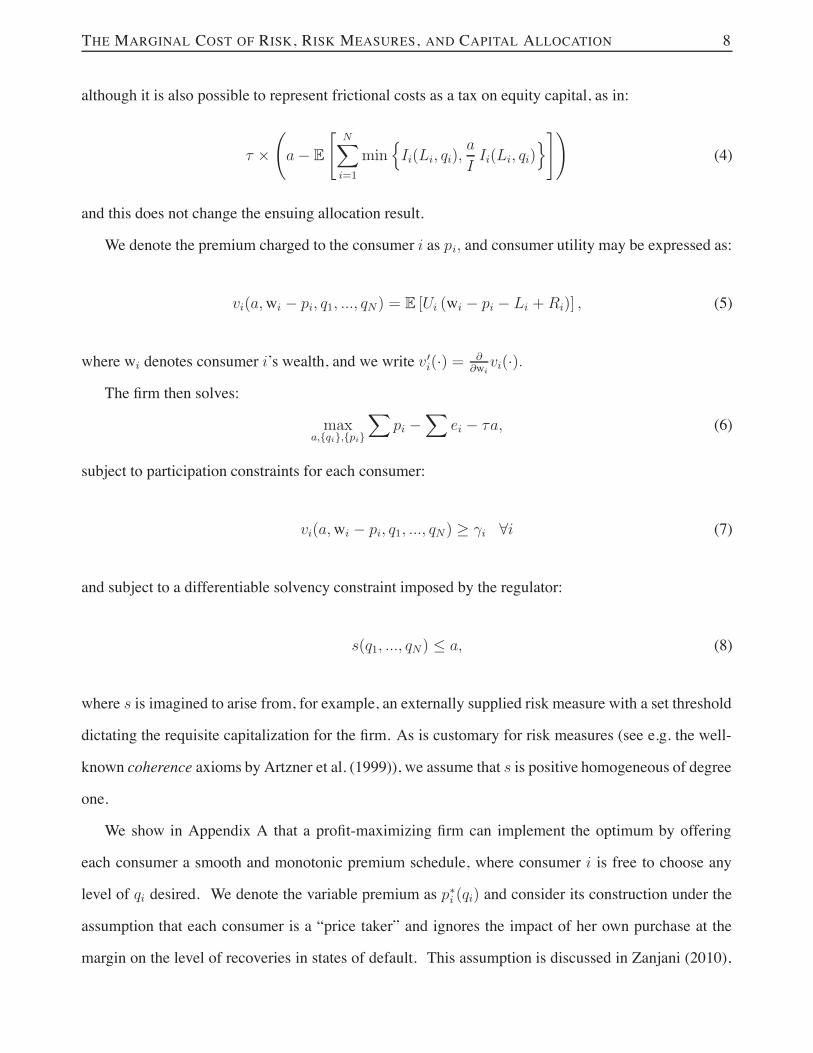
although it is also possible to represent frictional costs as a tax on equity capital, as in:
" $*a& E
+N!
i=1
min"Ii(Li, qi),
a
IIi(Li, qi)
#,-(4)
and this does not change the ensuing allocation result.
We denote the premium charged to the consumer i as pi, and consumer utility may be expressed as:
vi(a,wi & pi, q1, ..., qN) = E [Ui (wi & pi & Li +Ri)] , (5)
where wi denotes consumer i’s wealth, and we write v "i(·) = !!wi
vi(·).
The firm then solves:
maxa,{qi},{pi}
!pi &
!ei & "a, (6)
subject to participation constraints for each consumer:
vi(a,wi & pi, q1, ..., qN) % #i 'i (7)
and subject to a differentiable solvency constraint imposed by the regulator:
s(q1, ..., qN) ( a, (8)
where s is imagined to arise from, for example, an externally supplied risk measure with a set threshold
dictating the requisite capitalization for the firm. As is customary for risk measures (see e.g. the well-
known coherence axioms by Artzner et al. (1999)), we assume that s is positive homogeneous of degree
one.
We show in Appendix A that a profit-maximizing firm can implement the optimum by offering
each consumer a smooth and monotonic premium schedule, where consumer i is free to choose any
level of qi desired. We denote the variable premium as p#i (qi) and consider its construction under the
assumption that each consumer is a “price taker” and ignores the impact of her own purchase at the
margin on the level of recoveries in states of default. This assumption is discussed in Zanjani (2010),

THE MARGINAL COST OF RISK, RISK MEASURES, AND CAPITAL ALLOCATION 9
who followed the transportation economics literature on congestion pricing (Keeler and Small (1977))
by using the assumption when calculating the optimal pricing function. With this assumption in place,
the marginal price change at the optimal level of qi must satisfy:
.$vi$qi
+ E.1{I!a} U
"i
a
I2Ii$Ii$qi
//& $vi$w
$p#i$qi
= 0 (9)
with U "i = U "
i (wi & pi & Li +Ri). The term in brackets represents how the consumer perceives the
marginal benefit of additional coverage, which, due to the aforementioned assumption, differs from the
true impact of coverage on the utility function by E01{I!a} U "
iaI2 Ii
!Ii!qi
1.
Appendix B.1 shows that (9) may be rewritten as:
$p#i$qi
=$eZi$qi
+$s
$qi
+P(I % a) + " &
!
k
!vk!a
v"k
,+ %i $ a$
+!
k
!vk!a
v"k
,, (10)
where
%i =E01{I!a}
2k
U !k
v!k
1I2 Ik
!Ii!qi
1
E01{I!a}
2k
U !k
v!k
IkI
1 . (11)
The last two terms of (10) imply an allocation of the marginal unit of capital to consumer that “adds
up.” More specifically, it can be verified that:
a$!
%i qi = a, (12)
whereas the regulatory constraint “adds up” by the homogeneity assumption:
! $s
$qiqi = a. (13)
Thus, the optimal marginal pricing condition (10) can be extended to fully allocate all of the firm’s
costs, including the cost of capital:
! $p#i$qi
qi =! $eZi
$qiqi + [P(I % a) a+ "a] .

THE MARGINAL COST OF RISK, RISK MEASURES, AND CAPITAL ALLOCATION 10
Note that the cost of capital as captured in the bracketed term breaks down as:
[P(I % a) a+ "a] =!
i
$s
$qiqi $
+P(I % a) + " &
!
k
!vk!a
v"k
,+!
i
%i qi $ a$+!
k
!vk!a
v"k
,.
So an individual consumer’s capital allocation has two components. The first derives from an “internal”
marginal cost—driven by the cross-effects of consumers on each other:
%i qi $ a$+!
k
!vk!a
v"k
,
and the second originates from an “external” marginal cost imposed by regulators:
$s
$qiqi $
+P(I % a) + " &
!
k
!vk!a
v"k
,.
It is useful at this point to consider several different institutional scenarios.
Full Coverage by Deposit Insurance and Binding Regulation
If consumers are fully covered by deposit insurance, they are indifferent to the capitalization of their
financial institution. Mathematically, this means that:
!
k
!vk!a
v"k= 0,
so that (10) becomes:$p#i$qi
=$eZi$qi
+$s
$qi[P(I % a) + " ] . (14)
Thus, the marginal cost of risk, and the attendant allocation of capital, is completely determined by the
gradient of the binding regulatory constraint. This is the world of Denault (2001), Tasche (2004) and
others involved in the development of the gradient allocation principle. In this world, the marginal cost
of risk is indeed completely determined by an arbitrarily chosen risk measure.

THE MARGINAL COST OF RISK, RISK MEASURES, AND CAPITAL ALLOCATION 11
No Deposit Insurance and Non-Binding Regulation
At the opposite extreme is the case of an unregulated market with no deposit insurance. Here, Con-
straint (8) is immaterial, so (cf. Eq. (47) in Appendix B.1):
!
k
!vk!a
v"k= [P(I % a) + " ] ,
meaning that (10) becomes:
$p#i$qi
=$eZi$qi
+ %i $ a$ [P(I % a) + " ] . (15)
Thus, the marginal cost of risk and the attendant allocation of capital is driven completely by “internal”
considerations. Specifically, (11) indicates that the allocation is driven by the time-zero value that
consumers place on their anticipated recoveries in the various states of default.
General Case: Uninsured Consumers and Binding Regulation
In general, we may imagine the case where both of the considerations isolated above—an “external”
regulatory constraint, and “internal” concerns driven by counterparty preferences—are influencing the
marginal cost of risk. In this case, (10) remains in its original form:
$p#i$qi
=$eZi$qi
+$s
$qi
+P(I % a) + " &
!
k
!vk!a
v"k
,+ %i $ a$
+!
k
!vk!a
v"k
,, (16)
but we are now able to see more clearly the two influences on capital allocation. When the regulatory
constraint binds, we know that:
P(I % a) + " >!
k
!vk!a
v"k,
with the interpretation that regulation is forcing the institution to hold assets beyond the level that
would be privately efficient from the perspective of serving its counterparties. The extent of this
distortion is the key to whether internal counterparty concerns or external regulatory concerns guide

THE MARGINAL COST OF RISK, RISK MEASURES, AND CAPITAL ALLOCATION 12
capital allocation. If regulation comes close to replicating the private market outcome:
P(I % a) + " )!
k
!vk!a
v"k,
then the second term in (10) will be unimportant relative to the third term, and internal counterparty
concerns will dominate. On the other hand, if regulation pushes institutional capitalization well beyond
the level that would prevail in the private market:
P(I % a) + " *!
k
!vk!a
v"k,
then the second term in (10) overshadows the third, and external regulatory concerns dominate.
2.2 Allocation in a Security Market Equilibrium
To keep the setup simple, we limit our considerations to a one-period market with a finite number of
securities (M), each security with potentially distinct payoffs in X states and assume that the risk-free
rate is zero. More specifically, let !(S) = {!(S)1 , . . . ,!(S)
X } be the set of these states with associated
sigma-algebra F (S) given by its power set and let p(S)j = P3{!(S)
j }4denote the associated (physical)
probabilities. Let thenD be theM $X matrix withDij describing the payoff of the ith security in state
!(S)j , where we assume:
span(D) = RX .
This condition allows us to define unique state prices, consistent with the absence of arbitrage within
the securities market, denoted by &j , j = 1, . . . , X. Thus, any arbitrary menu of securities-market-
sub-state-contingent consumption can be purchased at time zero. However, it would be misleading to
characterize markets as complete, since !(S) does not provide a complete description of the “states of
the world.” Instead, we characterize the full probability space as5!, F ,P
6, with:
! = !(S) $ ! =7! = (!(S),!)
88!(S) # !(S), ! # !9,

THE MARGINAL COST OF RISK, RISK MEASURES, AND CAPITAL ALLOCATION 13
F = F (S) + F , and
P5A6
=!
j$!A
p(S)j $ P3Aj
888{!(S)j }4
for A =:
j$!A{!(S)
j }$Aj # F with Aj # F , j = 1, 2, . . . , |#A|.
Our problem now, however, is that the market is no longer complete so that we need a notion of
what insurance liabilities are “worth” to the insurer when they cannot be hedged completely. We make
the assumption that the insurance market is “small” relative to the securities market and, for purposes
of valuing insurance liabilities, employ the so-called minimal martingale measure: 7
Q5A6=!
j$!A
&j $ P3Aj
888{!(S)j }4, A , !,
i.e. Q is defined by the Radon-Nikodym derivative !Q!P ((!(S)j ,!)) = "j
p(S)j
.
Consumer utility now depends on the individual’s chosen security market allocation:
vi = EP [Ui (Wi & pi & Li +Ri)] with v"i = EP [U "i (Wi & pi & Li +Ri)] ,
whereWi is F (S)-measurable with wij = Wi(!(S)j ) and
2j &j wij = wi, whereas Li is F -measurable.
The recoveryRi now depends both on insurance loss activity as well as portfolio decisions made within
the insurance company. To elaborate on this, the budget constraint of the insurance company may be
expressed as:
a =!
j
&j Kj a - 1 =!
j
&j Kj ,
where Kj a reflects consumption purchased in the securities market state ! (S)j or—more precisely—in
the states of the world !j ="! = (!(S),!)
88!(S) = !(S)j
#. We write K to denote the corresponding
7As indicated by Bjork and Slinko (2006), the minimal martingale measure “provides us with a canonical benchmarkfor pricing.” It emerges as the optimal martingale measure given various criteria proposed in the mathematical financeliterature if the market for insurance risk is “small” relative to financial markets, i.e. if these risks do not affect the payoffof financial securities (see e.g. Goll and Ruschendorf (2001) or Henderson et al. (2005)), and it has also appears in othersettings throughout the finance literature. For instance, the minimal martingale measure coincides with the “hedge-neutralmeasure” in Basak and Chabakauri (2006), and it arises as the limit of Cochrane and Saa-Requejo price bounds for Ito priceprocesses as shown by Cerny (2003). We refer to Follmer and Schweizer (2010) for a formal definition.

THE MARGINAL COST OF RISK, RISK MEASURES, AND CAPITAL ALLOCATION 14
F (S)-measurable random variable. Consumer i’s recovery can then be expressed as:
Ri = min
;Ii,
K a
IIi
<,
and the fair valuation of claims is thus:
ei = EQ [Ri] = EQ $Ri 1{I<K a}%
& '( )=eZi
+EQ $Ri 1{I!K a}%
& '( )=eDi
.
As before, we can now derive the capital allocation according to the company’s marginal cost by
working through its optimization problem (see Appendix B.2 for details). We obtain an allocation result
similar to that of the previous section: The cost of capital:
$EQ $K a1{I!K a}
%+ " a
%,
which now reflects state prices and the company’s asset allocation, can be decomposed according to
the marginal costs for each of the individual exposures as:
0EQ $K a1{I!K a}
%+ ! a
1=!
i
"s
"qiqi
+
EQ $K 1{I!K a}%+ ! &
!
k
!vk!a
v"k
,
+!
i
#i qi a$+!
k
!vk!a
v"k
,
,
(17)
where:
#i =EQ01{I!K a}
2k
U !k
EP[U !k|#(S)]
KI2 Ik
!Ii!qi
1
EQ01{I!K a}
2k
U !k
EP[U !k|#(S)]
K IkI
1 =
2j $j Kj EP
.1{I!Kj a}
2k
U !k
EP[U !k|#
(S)j ]
IkI
!Ii!qiI
8888%(S)j
/
2j $j Kj EP
.1{I!Kj a}
2k
U !k
EP[U !k|#
(S)j ]
IkI
8888%(S)j
/ .
(18)
Thus, we essentially have the same result as before, although the “internal” allocation rule now only
applies in every “branch” of the security market where the incompleteness becomes material. In par-
ticular, after adjusting for state prices by conditioning on each “branch,” capital allocation weights are
still determined by consumer marginal utility.
In the limiting case of a complete market (i.e. the case when Li and Ri are F (S)-measurable so that

THE MARGINAL COST OF RISK, RISK MEASURES, AND CAPITAL ALLOCATION 15
we can write lij = Li(!(S)j ) and rij = Ri(!
(S)j ), lij, rij # R) we obtain:
%i =EQ01{I!K a}
2k
KI2 Ik
!Ii!qi
1
EQ$K 1{I!K a}
% =
EQ.K
!Ii!qiI
8888 I % K a
/
EQ [K| I % K a], (19)
so that:
qi $ %i $ EQ $K a1{I!K a}%= EQ
.K a
IIi 1{I!K a}
/
is the fair price of the recovery. This result—where capital is allocated to consumers in proportion to
their share of the total market value of recoveries—is the same allocation result as in Ibragimov, Jaffee,
and Walden (2010). It is important to note, however, that in the complete market case, purchasing
protection from an insurance company with costly capital is inefficient since consumers can hedge
insurance risk themselves.8
2.3 A Multi-Period Version of the Model
In this section, we consider a generalization of the (one-period) setup to multiple periods. Let Lti
denote the loss incurred by consumer i, i # {1, 2, . . . , N}, in period t, t # {1, 2, . . .}. We assume
that Lti, t > 0—for fixed i—are independent and identically distributed, and we define the relevant
filtration F = (Ft)t!0 via Ft = '(Lsi , i # {1, 2, . . . , N}, s ( t). The firm determines the optimal
level of assets, at, in the beginning of each period (i.e. (at) is F-predictable) for a period cost of " $ at.
Similarly to before, the company chooses F-predictable amounts q it in I ti = I(Lti, q
ti) = qti $ Lt
i and
prices pti at the beginning of the period, and we denote the total claims by I t =2N
j=1 Itj .
Now the company defaults if I t > at, so that the recovery paid to each consumer is Rti =
min{I ti , atIt I
ti} and the company shuts down in case of default, i.e. shareholders do not have access
8Ibragimov, Jaffee, and Walden (2010) deal with this by assuming “the insurees do not have direct access to the marketfor risk” whereas the insurer faces a “friction-free complete market for risk.”

THE MARGINAL COST OF RISK, RISK MEASURES, AND CAPITAL ALLOCATION 16
to future profits.9 The consumer’s utility in period t is given by:
vti(at,wti & pti, q
t1, . . . , q
tN) = Et%1
$Ui(wt
i & pti & Lti +Rt
i)%,
where for simplicity we assume that wealth is homogeneous across periods, i.e. wti . wi.10
The company solves:
max{at},{qti},{pti}
V0 =&!
t=1
E+1{I1'a1,...,It"1'at"1} $
*!
i
pti &!
i
Et%1
$Rt
i
%& " at
-,(20)
with constraints:
vti(at, wti & pti, q
t1, . . . , q
tN) % #i 'i, 't, (21)
s(qt1, . . . , qtN) ( at 't. (22)
Under the assumptions above, it is clear that there exists an optimal stationary policy:
(at, {qti}, {pti}) . (a#, {q#i }, {p#i })
that solves the Bellman equation:
V = maxa,{qi},{pi}
!
i
pi &!
i
E[Rti]& '( )
ei
&" a+ P[I t ( a]$ V (23)
under conditions (21) and (22). Hence, we have a similar program as in the basic setup from Section
2.1 before, where the primary difference is the last term in (23) involving the value function.
Proceeding analogously to before (see Appendix B.3 for details), we obtain the following marginal9Alternatively, it is possible to allow the distressed company to raise additional funds in the case of default at a higher
(or even increasing) cost akin to Froot, Scharfstein, and Stein (1993) and Froot and Stein (1998). Here, we limit ourconsiderations to this simple case and leave the further exploration of alternative settings for future research.
10Formally, the consumers will form utilities over consumption in multiple periods. In particular, future (random) losseswill also be material. Thus, hereU should rather be interpreted as a value function (of end-of-periodwealth) than as a utilityfunction (of end-of-period consumption).
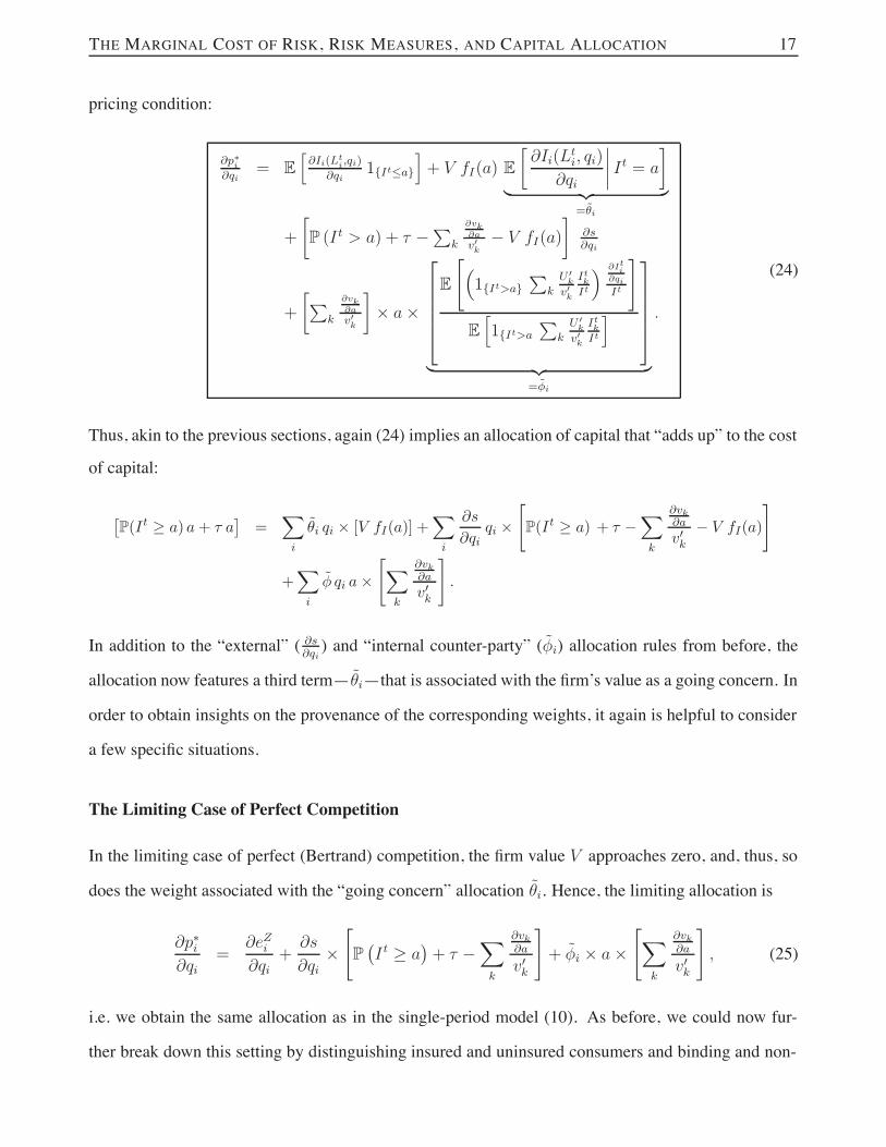
THE MARGINAL COST OF RISK, RISK MEASURES, AND CAPITAL ALLOCATION 17
pricing condition:
!p#i!qi
= E0!Ii(Lt
i,qi)!qi
1{It'a}
1+ V fI(a) E
.$Ii(Lt
i, qi)
$qi
8888 It = a
/
& '( )=$i
+
.P (I t > a) + " &
2k
!vk!av!k
& V fI(a)
/!s!qi
+
.2k
!vk!av!k
/$ a$
=
>>>>?
E+3
1{It>a}2
kU !k
v!k
ItkIt
4 !Iti!qiIt
,
E01{It>a
2k
U !k
v!k
ItkIt
1
@
AAAAB
& '( )=%i
.
(24)
Thus, akin to the previous sections, again (24) implies an allocation of capital that “adds up” to the cost
of capital:
$P(It % a) a+ ! a
%=!
i
&i qi $ [V fI(a)] +!
i
"s
"qiqi $
+P(It % a) + ! &
!
k
!vk!a
v"k& V fI(a)
,
+!
i
# qi a$+!
k
!vk!a
v"k
,.
In addition to the “external” ( !s!qi ) and “internal counter-party” (%i) allocation rules from before, the
allocation now features a third term—(i—that is associated with the firm’s value as a going concern. In
order to obtain insights on the provenance of the corresponding weights, it again is helpful to consider
a few specific situations.
The Limiting Case of Perfect Competition
In the limiting case of perfect (Bertrand) competition, the firm value V approaches zero, and, thus, so
does the weight associated with the “going concern” allocation (i. Hence, the limiting allocation is
$p#i$qi
=$eZi$qi
+$s
$qi$+
P5I t % a
6+ " &
!
k
!vk!a
v"k
,
+ %i $ a$+!
k
!vk!a
v"k
,
, (25)
i.e. we obtain the same allocation as in the single-period model (10). As before, we could now fur-
ther break down this setting by distinguishing insured and uninsured consumers and binding and non-

THE MARGINAL COST OF RISK, RISK MEASURES, AND CAPITAL ALLOCATION 18
binding regulation to obtain allocations that are fully determined by “external” and “internal counter-
party” considerations, respectively. In particular, in this case the remaining two weights in (25) adhere
to the same interpretation as in the single period setting.
Monopolistic Competition, Full Coverage by Deposit Insurance, and Non-Binding Regulation
In this case, again consumers are indifferent to the capitalization of the firm and there is no external
solvency constraint, so that the level—and the allocation—of firm capital is solely determined by the
firm’s value as a going concern:
$p#i$qi
= E.$Ii(Lt
i, qi)
$qi1{It'a}
/+ V fI(a)E
.$Ii(Lt
i, qi)
$qi
8888 It = a
/
= E.$Ii(Lt
i, qi)
$qi1{It'a}
/+$P5I t > a
6+ "%$ E
.$Ii(Lt
i, qi)
$qi
8888 It = a
/, (26)
where the latter equality follows from the first order condition for a in the absence of constraints (see
Eq. (52) in Appendix B.3).
General Case: Monopolistic Competition, Uninsured Consumers, and Binding Regulation
Here we obtain (24) and can now identify the three influences on capital allocation. Two are exactly the
same as before—with their relative importance determined by how close the regulatory requirement is
to the capitalization level chosen by the consumers in an unregulated market. The relative importance
of the “new” term (i that derives from the firm’s value as a going concern depends on how different the
capitalization would be if regulatory and consumer concerns were immaterial. In particular, if consumer
and shareholder considerations in a private (unregulated) market would yield a similar capitalization as
imposed by regulation:
P(I t % a) + " )!
k
!vk!a
v"k+ V fI(a),
then internal counterparty and continuation value concerns will dominate whereas regulatory concerns
will be the key driver otherwise.
Inspecting the form of the regulatory and the shareholder-driven allocation, they are reminiscent of

THE MARGINAL COST OF RISK, RISK MEASURES, AND CAPITAL ALLOCATION 19
conventional allocation methods based on the gradients of risk measures. The next section elaborates
on these relationships in more detail.
3 Capital Allocation and Risk Measures
The “black board solution” of Section 2 offers little obvious consolation to a practitioner faced with the
problem of allocating capital in a real-world setting, as it may seem difficult to implement. Indeed, the
popularity of allocation methods based on risk measures, particularly the so-called Euler or Gradient
allocation, can be attributed in part to its ease of application. However, there has been little scientific
analysis of the question of how to choose risk measures for the purposes of capital allocation. Conven-
tional thinking points to the various mathematical properties of risk measures (e.g., coherence), yet it
is not clear whether choices made on such a basis yield economically desirable outcomes (see Grundl
and Schmeiser (2007)).
This section aligns our results with those obtained from the Euler method. We first formally intro-
duce the Euler allocation principle. We then derive the risk measures which—if the Euler method were
applied to them—would yield our allocation results.
3.1 The Euler Allocation Principle
Although it is not always derived in this way, the Euler method is implied by the maximization of profits
subject to a risk measure constraint. To illustrate, assume a company’s profit function $ depends on
the parameters (volumes) qi, 1 ( i ( N, and on capital a. Then maximizing profits subject to the risk
measure constraint:
) (q1, q2, . . . , qN) *& ( a
yields:$$
$qi=
C&$$$a
D*&$)
$qi
at the optimal values a#, q#i , 1 ( i ( N. Here ) is a differentiable risk measure evaluated at the aggre-
gate claims2N
j=1 Ij(Lj, qj) and *& is an exchange rate that converts risk to capital (which is set at one if

THE MARGINAL COST OF RISK, RISK MEASURES, AND CAPITAL ALLOCATION 20
risk is measured in monetary units—i.e. in the case of a monetary risk measure). Hence, for the optimal
portfolio, the risk-adjusted marginal return on marginal capital !"/!qi'"(!&/!qi for each exposure is the same
and equals the cost of a marginal unit of capital & !"!a . In other words, if the marginal performance of
risk i as measured by its marginal return on marginal risk capital *& $ !&!qiexceeds (respectively, falls
below) the cost of a marginal unit of capital, then increasing (respectively, decreasing) the weight qi of
that exposure by a small amount improves the overall performance of the portfolio.11 Akin to the results
of Tasche (2004) on the suitability of capital allocation principles, this motivates the interpretation of
the marginal capital weighted by the corresponding volume *& !&!qi q#i as the amount of capital allocated
to exposure i. For homogenous risks and risk measure, the allocations to the respective risks “add up”
to the entire capital:N!
j=1
*&$)
$qjq#j = a#.
We refer to McNeil, Frey, and Embrechts (2005) and references therein for more details on the
Euler principle, and to Denault (2001), Kalkbrener (2005), and Myers and Read (2001) for alternative
derivations of the Euler principle based on cooperative game theory, formal axioms, or a contingent
claim approach, respectively. Regardless of its provenance, the Euler method’s strength is the feasibility
of implementation, as it is only necessary to calculate the partial derivatives of a given risk measure
with respect to each exposure evaluated at the current portfolio.
3.2 Allocation Based on Risk Measures
We now proceed to derive the risk measures that correspond to the capital allocations derived in Sec-
tion 2. Each of the three components of capital allocation are associated with a unique risk measure.
The first component of capital allocation—that associated with the external risk measure—maps
obviously as the output of the Euler method applied to that external risk measure. To illustrate, when
consumers are fully insured by deposit insurance (and perfect competition prevails in the multi-period
context), the only relevant constraint on risk-taking derives from the given risk measure s— so that11Cf. Section 6.3.3 “Economic Justification of the Euler Principle” in McNeil, Frey, and Embrechts (2005).
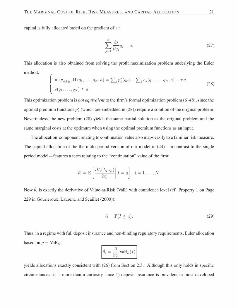
THE MARGINAL COST OF RISK, RISK MEASURES, AND CAPITAL ALLOCATION 21
capital is fully allocated based on the gradient of s :
N!
j=1
$s
$qjqj = a. (27)
This allocation is also obtained from solving the profit maximization problem underlying the Euler
method: EFG
FH
maxa,{qi}$ (q1, . . . , qN , a) =2
k p#k(qk)&
2k ek(q1, . . . , qN , a)& " a,
s(q1, . . . , qN) ( a.(28)
This optimization problem is not equivalent to the firm’s formal optimization problem (6)-(8), since the
optimal premium functions p#i (which are embedded in (28)) require a solution of the original problem.
Nevertheless, the new problem (28) yields the same partial solution as the original problem and the
same marginal costs at the optimum when using the optimal premium functions as an input.
The allocation component relating to continuation value also maps easily to a familiar risk measure.
The capital allocation of the the multi-period version of our model in (24)—in contrast to the single
period model—features a term relating to the “continuation” value of the firm:
(i = E.$Ii(Li, qi)
$qi
8888 I = a
/, i = 1, . . . , N.
Now (i is exactly the derivative of Value-at-Risk (VaR) with confidence level (cf. Property 1 on Page
229 in Gourieroux, Laurent, and Scaillet (2000)):
+ = P(I ( a). (29)
Thus, in a regime with full deposit insurance and non-binding regulatory requirements, Euler allocation
based on ) = VaR(:
(i =$
$qiVaR((I)
yields allocations exactly consistent with (26) from Section 2.3. Although this only holds in specific
circumstances, it is more than a curiosity since 1) deposit insurance is prevalent in most developed

THE MARGINAL COST OF RISK, RISK MEASURES, AND CAPITAL ALLOCATION 22
banking and (primary) insurance markets and 2) regulatory capital requirements—though common in
intermediary markets—frequently do not bind, i.e. solvency ratios exceed the required level (see e.g.
Hanif et al. (2010)).
To motivate the measure corresponding to the “internal counterparty” component of capital allo-
cation, consider now a company in a regime without (full) coverage by deposit insurance (but still
assume perfect competition in the multi-period context). Then, capitalization will become material to
consumers—which mathematically corresponds to the %i’s emerging in the marginal cost allocations
(10)/(24), where:
%i =
E.1{I!a}
2k
U !k
v!k
IkI
!Ii!qiI
/
E01{I!a}
2k
U !k
v!k
IkI
1 .
To align this allocation with the Euler method, introduce the probability measure P on (!,F) via
its Radon-Nikodym derivative:
$P$P =
2k
U !k
v!k
IkI 1{I!a#}
E02
kU !k
v!k
IkI 1{I!a#}
1 , (30)
where I , U , etc. are evaluated at the concurrent (optimal) values a#, p#i (q#i ), q#i , 1 ( i ( N. Note that
P is absolutely continuous with respect to the original probability measure P but the measures are not
equivalent since under P all the probability mass is concentrated in default states. On the set of strictly
positive P-square integrable random variables:
L2+
3!,F , P
4="X # L2
3!,F , P
4|X > 0 P-a.s.
#,
we define the risk measure:12
)(X) = exp"EP [log{X}]
#. (31)
Obviously ) is monotonic ()(X) ( )(Y ) forX ( Y a.s.), positive homogenous ()(aX) = a )(X),
a > 0), and it satisfies the constancy condition )(c) = c for c > 0 (see Frittelli and Gianin (2002) for a
discussion of properties of risk measures). However, ) is neither translation-invariant nor sub-additive12While its functional form seems similar to that of the so-called entropic risk measure, which has recently gained
popularity in the mathematical finance literature (see e.g. Follmer and Schied (2002) or Detlefsen and Scandolo (2005)),note that the roles of the exponential function and the logarithm are interchanged.

THE MARGINAL COST OF RISK, RISK MEASURES, AND CAPITAL ALLOCATION 23
and is therefore not coherent and not convex. In fact, ) is not even a monetary risk measure and thus
may seem ill-suited for use as an external risk measure.13 Nevertheless, in our setting, it is the correct
risk measure for internal capital allocation based on the Euler principle.
More precisely, define *& = a#
&(!N
j=1 Ij(Lj ,q#j ))as the “exchange rate” between units of risk and
capital. Then the application of the Euler principle with profit function $ (q1, . . . , qN , a) as in (28) and
risk measure constraint:
)
*N!
j=1
Ij(Lj , qj)
-
& '( )=&(q1,...,qN )
*& ( a, (32)
yields:
N!
j=1
*&$)
$qjq#j [P(I % a#) + " ] =
N!
j=1
*& EP.$Ij/$qj
I
/) q#j [P(I % a#) + " ] (33)
=N!
j=1
%j q#j a
# [P(I % a#) + " ] = a# [P(I % a#) + " ] ,
which is exactly the allocation (15) derived in the previous section.14 While it may appear problematic
to use the optimal levels a# and q#i in the definition of *& and the Radon-Nikodym derivative !P!P , note
that this is akin to employing the optimal premium functions p# for deriving the Euler allocation based
on the externally supplied risk measure within the first component described above. Just like there,
optimizing $ subject to the risk measure constraint (32) is a simple auxiliary problem that yields the
same partial solution and the same capital allocation as the firm’s full optimization problem. Moreover,
by inserting the definition of *&, we obtain a more familiar representation of the amount of capital
allocated to consumer i (cf. Schmock and Straumann (1999)):
a# $ q#i $!&!qi
(q#1, . . . , q#N)
)(q#1, . . . , q#N)
.
Hence, the correct internal capital allocation according to marginal cost can be implemented by the13While sub-additivity is subject of an ongoing debate (see e.g. Dhaene et al. (2008) or Kou, Peng, and Heyde (2012)),
at least translation invariance is generally deemed adequate for an external risk measure and even “necessary for the risk-capital interpretation [...] to make sense” (see p. 239 in McNeil, Frey, and Embrechts (2005)).
14In a setting with securities markets (Eq. (18)), the risk measure still takes the same form (31) but state prices andallocations to security market states enter the measure transform (30).

THE MARGINAL COST OF RISK, RISK MEASURES, AND CAPITAL ALLOCATION 24
Euler principle relying on the risk measure ).
General institutional circumstances—i.e., binding regulation, imperfect competition, and incom-
plete deposit insurance—will lead to a risk measure that combines the three foregoing risk measures.
In the general case from Section 2.3, the allocation can be rewritten as:
N!
j=1
$s
$qjq#j
+
P(I % a#) + " &!
k
!vk!a
v"k& V fI(a
#)
,
+N!
j=1
*&$)
$qjq#j
+!
k
!vk!a
v"k
,+
N!
j=1
$VaR(#$qj
q#j [V fI(a#)] = a# [P(I % a#) + " ] ,
so that:N!
j=1
$
$qj((1& ,1 & ,2) s+ ,1 *& )+ ,2VaR(#) q#j = a#,
where:
,1 =
2k
!vk!av!k
P(I % a#) + ",
,2 =V fI(a#)
P(I % a#) + ".
Hence, the Euler principle can still be applied, but the supporting risk measure is a weighted average
of the external risk measure s, the internal risk measure ), and VaR. The weights on the latter two
measures are determined by the consumers’ and the shareholders’ preferences for capitalization of the
company at the margin and are dictated by the considerations outlined in Section 2.3.
4 Comparison of Capital Allocation Methods
This section shows how the counterparty-driven internal allocation effectively differs from the alloca-
tion based on ES—perhaps the most widely endorsed measure within the academic and practitioner
communities—in the context of two single-period examples. In particular, we are interested in how
the economic weight assigned to various outcomes and various risks under ) differs from what would
be obtained from applying the Euler technique to ES.

THE MARGINAL COST OF RISK, RISK MEASURES, AND CAPITAL ALLOCATION 25
4.1 The Case of Homogeneous Exponential Losses
Assume that there are N identical, independent consumers with wealth level w in a regime with non-
binding regulation that face independent, Exponentially distributed losses L i / Exp(-), 1 ( i ( N .
Assume further that all consumers exhibit a constant absolute risk aversion of + < -, and that their
participation constraint is given by the autarky level:
# = #i = E [U(w& Li)] = &e%(w-
- & + .
Then, the firm’s optimization problem in the one period model without a regulatory constraint (6)/(7)
may be represented as:
EFFFFFFFFFFFG
FFFFFFFFFFFH
maxa,q,p
;N $ p&N $ q $
.1)%N%1,)
3aq
4& )N"1
(N%1)!e%) a
q
3aq
4N%1 31) +
1N
aq
4/
&a$ %N,)
3aq
4& " $ a
#
subject to
# ( e%((w%p)"
))%(1%q)(
0%N%1,)
3aq
4& e
" aq (#"(1"q)$)
)N"1
((1%q)()N"1 %N%1,(1%q)(
3aq
41
+2&
k=0
5()
6k (N%1)!(N%1+k)!e
%) a2N%1j=0
(a ))j
j!(N%j+k%1)!(N%j%1)! %N%j+k,)
3a3
1%qq
44#,
(34)
where %m,b(x) = 1 & %m,b(x) and %m,b(·) denotes the cumulative distribution function of the Gamma
distribution with parametersm and b (see the Appendix C.1 for the derivation of (34)).
Note that the premiums pi . p and the coverage amounts qi . q are equal for all consumers since
they are identical. Likewise, any reasonable allocation rule trivially yields identical allocations for each
consumer, and particularly:
q %i = N%1, i = 1, 2, . . . , N,
for the counterparty-driven allocation—rendering a comparison to other allocation methods moot.
However, we may analyze how different allocations arrive at this congenerous result, i.e. we can distin-
guish different allocation methods by comparing the weight they put on different loss states.
For instance, for the allocation based on the Expected Shortfall (ES) according to the Euler princi-

THE MARGINAL COST OF RISK, RISK MEASURES, AND CAPITAL ALLOCATION 26
ple, it is well known that (see e.g. McNeil, Frey, and Embrechts (2005)):15
1
N=
aESia
=qE [Li| q L % a]
E [I| I % a]=
E [E[Li|L]| q L % a]
E [L| q L % a]=
1
NE [const$ L| q L % a] ,
where L =2
j Lj , i.e. the Expected Shortfall can be associated with a linear weighting function of the
default states.
For the counterparty-driven allocation, on the other hand, we obtain:
1
NEq. (11)=
E001{qL!a}
2Nj=1U
"3w& p& Lj + aLj
L
4Lj
L
1LiL
1
E01{qL!a}
2Nj=1 U
"3w& p& Lj + aLj
L
4Lj
L
1
= EP.Li
L
/=
1
NE+E+$P$P
88888L,
& '( )*(L)
,, (35)
i.e. the weighting function is implied by the measure transform and can be expressed as:
.(l) = 1{ql!a} cN,),(,a,q
&!
k=0
(k + 1) (+(l & a))k
(N + k)!, (36)
where cN,),(,a,q is a constant ensuring that E0.(L)
1= 1.16
In particular, for the risk measure ) evaluated at the aggregate loss I , we have:
)(I) = )(q L) = exp"E0.(L) log{qL}
1#= exp
"E0.(L) log{qL}
888 qL % a1#
, (37)
with .(l) = P(qL % a)$ .(l). Thus, ) in this sense is in fact a tail risk measure, and hence is related
to ES. The weights .(·) perform a role similar to the risk spectrum within the so-called spectral risk
measures as introduced in Acerbi (2002). However, while there the risk spectrum purports to encode
the “subjective risk aversion of an investor” to justify overweighting bad outcomes, in our setting15As in Section 3.2, to compare results we assume that the confidence level is chosen according to the outcome of the
firm’s optimization problem, i.e. ' = P(q L % a).16The derivation of these equations, a closed form solution for cN,!,",a,q as well as a representation of ((·) not involving
an infinite sum for implementation purposes all are provided in Appendix C.2.

THE MARGINAL COST OF RISK, RISK MEASURES, AND CAPITAL ALLOCATION 27
the weights represent an adjustment to objective probabilities based on the value placed by claimants
on recoveries in various states of default. Thus, the pivotal characteristics for our weights lie in the
primitives of the firm’s profit maximization problem (namely, the preferences of counterparties)—
which ultimately determine the overall choice of capitalization as well as the values consumers place
on state contingent recoveries—rather than in a subjectively specified preference function for the firm.
In the absence of weights, the concavity of the logarithmic function will, in the course of the ap-
plication of the Euler allocation methods, tend to penalize bad outcomes less heavily than ES. In fact,
it is evident from (35) that for .(·) . 1, the counterparty-driven allocation will effectively weight all
aggregate loss outcomes in excess of the firm’s capital equally, regardless of size. The reason for this is
that .(·) . 1 implies that the firm’s counterparties are risk-neutral (+ = 0 in (36)) and, thus, the value
of the firm in all states of default, regardless of how extreme the default, is simply the firm’s assets. At
the margin, the counterparties evaluate changes in risk simply from the perspective of how the expected
value of recoveries from the firm are affected, and recoveries in mild states of default are weighted no
differently from severe ones. This is also the reason why ) is not sub-additive or translation-invariant:
Adding a constant amount to the aggregate loss in high loss states is less precarious than in low loss
states because of limited liability.
Under risk aversion, on the other hand, .(·) 0= 1, and counterparties will weight recoveries in
severe states of default more heavily than mild ones. In fact, in the current setting .(·) is increasing and
strictly convex, and for all risk aversion levels + > 0 there exists a loss level l0 such that the weighting
function for the counterparty-driven allocation will exceed that of ES for all loss levels greater than l0.17
However, for smaller—and more probable—loss realizations, different shapes are possible rendering
either the ES-based allocation or the counterparty-driven allocation to appear more conservative.
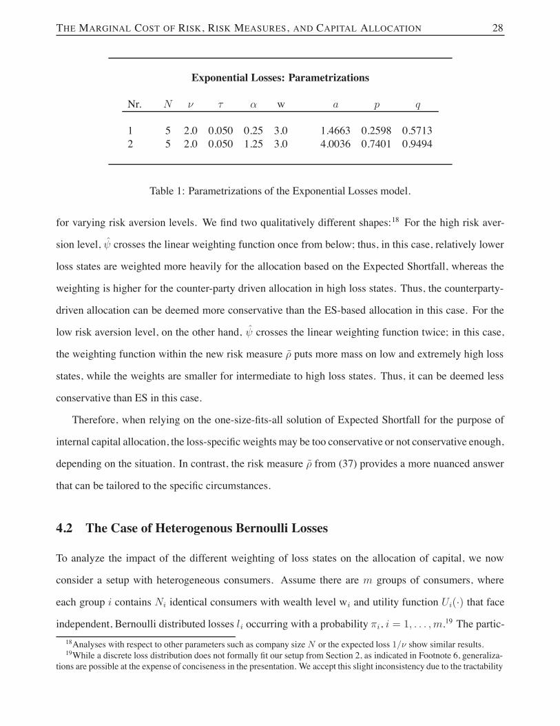
To analyze this relationship, in Table 1 we present two parametrizations of the setup and the corre-
sponding optimal parameters a, p, and q as solutions of the program (34) with different risk aversion
levels. The properties are as expected: a, p, and q all are increasing in risk aversion. Figure 1 plots
the weighting function . against the linear weighting function associated with the Expected Shortfall17It is worth noting that ((·) generally is not necessarily convex; it is possible to construct examples where the shape is
strictly concave or even linear.
THE MARGINAL COST OF RISK, RISK MEASURES, AND CAPITAL ALLOCATION 28
Exponential Losses: Parametrizations
Nr. N - " + w a p q
1 5 2.0 0.050 0.25 3.0 1.4663 0.2598 0.57132 5 2.0 0.050 1.25 3.0 4.0036 0.7401 0.9494
Table 1: Parametrizations of the Exponential Losses model.
for varying risk aversion levels. We find two qualitatively different shapes:18 For the high risk aver-
sion level, . crosses the linear weighting function once from below; thus, in this case, relatively lower
loss states are weighted more heavily for the allocation based on the Expected Shortfall, whereas the
weighting is higher for the counter-party driven allocation in high loss states. Thus, the counterparty-
driven allocation can be deemed more conservative than the ES-based allocation in this case. For the
low risk aversion level, on the other hand, . crosses the linear weighting function twice; in this case,
the weighting function within the new risk measure ) puts more mass on low and extremely high loss
states, while the weights are smaller for intermediate to high loss states. Thus, it can be deemed less
conservative than ES in this case.
Therefore, when relying on the one-size-fits-all solution of Expected Shortfall for the purpose of
internal capital allocation, the loss-specific weights may be too conservative or not conservative enough,
depending on the situation. In contrast, the risk measure ) from (37) provides a more nuanced answer
that can be tailored to the specific circumstances.
4.2 The Case of Heterogenous Bernoulli Losses
To analyze the impact of the different weighting of loss states on the allocation of capital, we now
consider a setup with heterogeneous consumers. Assume there are m groups of consumers, where
each group i contains Ni identical consumers with wealth level wi and utility function Ui(·) that face
independent, Bernoulli distributed losses li occurring with a probability &i, i = 1, . . . , m.19 The partic-18Analyses with respect to other parameters such as company size N or the expected loss 1/) show similar results.19While a discrete loss distribution does not formally fit our setup from Section 2, as indicated in Footnote 6, generaliza-
tions are possible at the expense of conciseness in the presentation. We accept this slight inconsistency due to the tractability

THE MARGINAL COST OF RISK, RISK MEASURES, AND CAPITAL ALLOCATION 29
0
1
2
3
4
5
0 1 2 3 4 5 6L
Par. 1ES
(a) ' = 0.25 – low loss levels
0
5
10
15
20
25
30
0 1 2 3 4 5 6L
Par. 2ES
(b) ' = 1.25 – low loss levels
0
5
10
15
20
25
30
0 5 10 15 20 25L
Par. 1ES
(c) ' = 0.25 – high loss levels
0
50
100
150
200
250
300
0 2 4 6 8 10L
Par. 2ES
(d) ' = 1.25 – high loss levels
Figure 1: Weighting function . for varying risk aversion parameter +.
ipation constraint again is given by their autarky levels:
#i = E [Ui(wi & Li)] = &i Ui(wi & li) + (1& &i)Ui(wi).
The optimization problem in the one period model without a regulatory constraint (6)/(7) can then be
conveniently set up by observing that the number of losses in the different groups follow independent
Binomial(Ni, &i) distributions.
For the counterparty-based allocation, we obtain for each consumer in group i:
qi #i = cN1!
k1=0
. . .Ni!
ki=1
. . .Nm!
km=0
I
J N1
k1
K
L . . .
I
J Ni & 1
ki & 1
K
L . . .
I
J Nm
km
K
L
$$k11 . . . $ki
i . . . $kmm (1& $1)
N1%k1 . . . (1& $i)Ni%ki . . . (1& $m)Nm%km
of the Bernoulli setup.

THE MARGINAL COST OF RISK, RISK MEASURES, AND CAPITAL ALLOCATION 30
$
=
?1{k1q1l1+...+kmqmlm!a}
EG
H
m!
j=1
kj U "3wj & pj & lj + qj lj
ak1q1l1+...+kmqmlm
4qj lj
v"j $ (k1q1l1 + . . .+ kmqmlm)
MN
O
@
B
& '( )=const(!P
!P
$ qi lik1q1l1 + . . .+ kmqmlm
, (38)
where c is a constant such that2
i Ni qi %i = 1. Thus, while the analytical form of the weights
.(I) = E0!P!P
888 I1is less transparent in this case, again we notice that they immediately depend on the
marginal utilities of recoveries in various states of default. For the allocation based on the Expected
Shortfall, on the other hand, we obtain for each consumer in group i:
aESia
= const $N1!
k1=0
. . .Ni!
ki=1
. . .Nm!
km=0
I
J N1
k1
K
L . . .
I
J Ni & 1
ki & 1
K
L . . .
I
J Nm
km
K
L
$$k11 . . . $ki
i . . . $kmm (1& $1)
N1%k1 . . . (1& $i)Ni%ki . . . (1& $m)Nm%km
1{k1q1l1+...+kmqmlm!a} qi li, (39)
i.e. it is of a similar form as (38) but now (a) does not contain the adjustment based on the marginal
utilities !P!P , and (b) the state-specific loss for a consumer in group i, (qi li), is not scaled by the aggregate
loss—which, in the counterparty-driven allocation, is a consequence of the proportional partitioning of
the recoveries in states of default.
To assess the consequences of these adjustments, we consider the case of two different types of
consumers with differing loss exposure and risk aversion levels. Specifically, we assume consumers
in the first group have wealth level w1 = 7, CARA preferences with an absolute risk aversion level
+1 = 1.75, and face a loss of size l1 = 2 occurring with a probability of &1 = 10%. Consumers in
the second group also have wealth w2 = 7, CARA preferences, and face a loss with an occurrence
probability of &2 = 10%, but we vary their risk aversion level +2 and the size of the loss l2. Figure 2
shows the optimal capital level, a, and the optimal coverage amount for consumers in group 2, q2, as a
function of +2 and l2 for group sizes N1 = N2 = 25 and capital cost " = 5%.
Unsurprisingly, Panel 2(a) shows that the optimal capital level is increasing in the loss level—which
of course is due to an increase in the expected loss. Moreover, we find that capital is also increasing in
the risk aversion level, which is due to a combination of two effects. On the one hand, more risk-averse

THE MARGINAL COST OF RISK, RISK MEASURES, AND CAPITAL ALLOCATION 31
2 2.5 33.5 4
4.5 55.5 6
6.5
00.5
11.5
22.5
3
10152025303540455055
Capital level a
l2'2
10152025303540455055
(a) Capital levels a
2 2.5 33.5 4
4.5 55.5 6
6.5
00.5
11.5
22.5
3
0.860.880.90.920.940.960.981
1.02
Amount q2
l2'2
0.860.880.90.920.940.960.9811.02
(b) Amounts q2
Figure 2: Optimal parameters a and q2 for group 2 loss levels l2 between between 2 and 6.5 and group2 risk aversion levels +2 between 0.25 and 2.95.
consumers are—ceteris paribus—more worried about nonperformance of their insurance contract and
thus prefer a higher level of capital. On the other hand, as is evident from Panel 2(b), higher risk
aversion levels prompt the consumers in group 2 to increase their coverage level q2, which in turn
increases expected losses.20
To demonstrate the influence of these effects on capital allocation, Figure 3 plots the difference in
the proportion of capital allocated to group 2 between the counterparty-based allocation rule, q2 %2,
and the ES allocation rule, aES2a , as a function of l2 and +2. From the figure, the functional relation-
ship appears to be non-smooth, which—aside from numerical errors—is due to genuine discontinuities
emerging from the discreteness of the resulting aggregate loss distribution. To better illustrate the un-
derlying relationships, we therefore include a 5$5-polynomial fit as well as contour lines based on the
smoothed surface.
To interpret the results, it is important to notice that the figure displays differences in allocations—
the absolute allocation levels vary much more across the different loss and risk aversion levels for both
allocation methods. For instance, for a risk aversion level of +2 = 1.75 and a loss level l2 = 6.5, the
proportion of capital allocated to consumers in group 2 based on ES is about 86.6% and about 87.5%
for the counterparty-based allocation principle, whereas for a risk aversion level +2 = 1.75 and loss20For the participation amount of consumers in group 1, q 1, we observe the opposite relationship, i.e. it is decreasing in
group 2 loss and risk aversion levels. The reason here is that—ceteris paribus—recoveries are larger and insurance is moreexpensive when the capital level is higher.

THE MARGINAL COST OF RISK, RISK MEASURES, AND CAPITAL ALLOCATION 32
l2 = 2, both allocations clearly yield 50% since the two consumer groups are identical in this case. In
particular, the difference between the two allocations is zero in the latter case as is also evident from
the corresponding contour line.
At first glance, the differences of about -1% for relatively low loss and risk aversion levels and about
2% for relatively large loss and risk aversion levels—resulting in an overall range of about 3% across all
combinations—appear rather small. However, it is important to note that with Bernoulli distributions
and group sizes of Ni = 25, diversification effects are very pronounced so that capital allocations
to each group are largely driven by their respective contributions to expected losses. Smaller group
sizes yield effects that are qualitatively similar but considerably larger; however, the aforementioned
discontinuities are also much more pronounced due to the discreteness of the loss distribution and
impede clear presentation of the primary effects.
234
56
0.511.522.5
-1.0%-0.5%0.0%0.5%1.0%1.5%2%
1.0%0.0$-0.5%
l2
'2
-1.5%-1.0%-0.5%0.0%0.5%1.0%1.5%2.0%2.5%
Figure 3: Difference in allocation of capital to group 2 between the counterparty-based allocation ruleand the ES allocation rule (q2 %2 & aES2
a ) for group 2 loss levels l2 between between 2 and 6.5 and group2 risk aversion levels +2 between 0.25 and 2.95.
As before, we find that the ES based allocations are too conservative—i.e. they put too much weight
on the group with the high risk consumers in group 2—if those consumers are not very risk averse
relative to group 1 consumers and the difference in loss sizes is relatively small. On the other hand, if

THE MARGINAL COST OF RISK, RISK MEASURES, AND CAPITAL ALLOCATION 33
group 2 consumers are relatively risk averse and face relatively large losses, the ES-based allocations
are not conservative enough—i.e. the counterparty-based principle allocates more capital to the high
risk group than ES.
5 Conclusion
The gradient allocation principle prescribes an allocation of capital to risks in the company’s portfolio
according to their marginal costs as defined via a given risk measure. However, risk measure selection is
a thorny issue that can be resolved only through careful consideration of institutional context—a prob-
lem implicitly recognized in the early literature on capital allocation (Myers and Read (2001), Tasche
(2004)—both of whom ultimately fall back on regulation as motivating the choice of risk measure) but
since overlooked in favor of a focus on mathematical properties of allocation rules and risk measures.
Instead of starting with a risk measure, this paper starts with primitive assumptions and calculates
the marginal cost of risk from the perspective of a profit-maximizing firm with risk averse counterpar-
ties. We then take the additional step of identifying the risk measure whose gradient yields allocations
consistent with marginal cost.
The resulting composite measure is a weighted average of three risk measures corresponding to
the interests of the different parties concerned with the capitalization of the firm: the regulator, share-
holders, and counterparties. The first risk measure relating to regulation is specified exogenously as
a part of the company’s optimization problem, while the risk measures corresponding to shareholder
and counterparty concerns arise endogenously in our setting. Shareholder concerns yield VaR whereas
counterparty concerns yield a novel risk measure, which can be expressed as the exponential of the ex-
pected value of the logarithm of the portfolio outcomes under an alternative probability measure which
reflects weights for counterparty preferences in default states. The composite risk measure will not
generally obey the principles of convexity or coherence. Nevertheless, it is the only one that yields the
appropriate allocation of capital for the profit-maximizing firm in our setting.
To obtain these theoretically economically correct allocations, one needs considerable information
to choose the appropriate weights as well as the probability transform encapsulated in the novel risk

THE MARGINAL COST OF RISK, RISK MEASURES, AND CAPITAL ALLOCATION 34
measure. That said, conventional risk measures also rely on selections for parameter values—such as
the confidence level in VaR or ES, or the weighting function in spectral risk measures—so from the
standpoint of practice the proposed measure starts from an economically sound foundation and offers
no greater level of complication than is already present. Moreover, as is evident from our numerical
applications, the parameters are structural, i.e. they correspond fundamental quantities, so they may be
calibrated according to the application in view.
We compare the allocations obtained in a single period setting without regulation to those obtained
from the gradient of ES—the coherent risk measure currently favored by many academics and regula-
tors. We show that ES may underweight or overweight severe states of default, depending on the nature
of customer risk aversion. This raises the interesting possibility that a transition away from a system of
regulation based on risk measure-based solvency assessment to one based on market (counterparty) dis-
cipline will not necessarily mitigate the oft-lamented failure of financial institutions to penalize “tail”
risk.
While the calculations in this paper are done from the perspective of a profit-maximizing firm, one
could also contemplate the calculus of a regulator or social planner. In specific cases, the calculus
will be similar. For example, a regulator without responsibility for unpaid losses (i.e., if no deposit
insurance scheme exists) but in a context where counterparties are uninformed will view risk similarly
to the profit-maximizing firm. However, a regulator responsible for unpaid losses would presumably
have to consider the value of unpaid losses in selecting a risk measure as well as other issues—such as
bankruptcy costs not internalized by private firms and the production cost technology associated with
deposit insurance—that would determine the optimal level of capitalization for financial institutions as
well as the social cost of risk. These issues are of course complex and well beyond the scope of this
paper, but they are intriguing areas for future research.

THE MARGINAL COST OF RISK, RISK MEASURES, AND CAPITAL ALLOCATION 35
Appendix
A Implementation of the Firm’s Optimization Problem via a Pre-mium Schedule
In the text we consider the solution of maximizing (6) subject to (7) and (8). We claim further that—ifthe consumer acts as a “price taker” with respect to the recovery rates offered by the company withinthe various states of default—that the company can implement the optimum by offering a smooth andmonotonically increasing premium schedule that allows each consumer to freely choose the level ofcoverage desired for the premium indicated by the schedule. It is subsequently shown (in AppendixB.1) that the marginal price increase associated with coverage must satisfy (10) when evaluated at theoptimum. It remains to be shown that this premium schedule exists and can be used to implement theoptimum.
A complication arises in modeling the consumer as a price-taker with free choice of coverage level.To introduce the consumer’s ignorance of his own influence on recoveries, we define price scheduledescribed above as p#i (·) and modify the original utility function to
vi (wi & p#i (qi), qi; a, q1, . . . , qN) = E0Ui
3wi & p#i (qi)& Li + Ri
41, (40)
where:
Ri = Ri (qi; a, q1, . . . , qN ) = min
PIi(Li, qi),
a2N
j=1 Ij (Lj , qj)Ii(Li, qi)
Q.
The idea here is to fix recovery rates by fixing the quantities a and {qi}, leaving the consumer with thefree choice of qi—but with the caveat that this choice does not influence recovery rates.21
The firm’s objective function is identical to the previous one, except that 1) the firm now specifiesa price function rather than a single price point, and 2) the firm fixes the recovery rates for purposes ofconsumer incentive compatibility by choosing a and {qi} instead of the “true” levels of a and {qi}:
maxa,{p#i (·)},{qi}
"!p#i (qi)&
!ei & " a
#(41)
The firm still faces the previous constraints (7) and (8),
vi (a,wi & p#i (qi), q1, . . . , qN) % #i,
s (q1, . . . , qN) ( a,
21Alternatively, we could also specify
ˆvi (wi & p!i (qi), qi; a, q1, . . . , qN ) = vi
Cwi & p!i (qi), qi;
qiqi
(a, q1, . . . , qN )
D,
where the consumer is cognizant of her own coverage but “scales” the company according to her own coverage level andthis would not change the presentation in the main text. Again, the important point is that the consumer expects the samerecovery per dollar of coverage in default states independent of her choice of q i.

THE MARGINAL COST OF RISK, RISK MEASURES, AND CAPITAL ALLOCATION 36
and in addition the new constraint:
qi # argmaxqi
vi(wi & p#i (qi), qi ; a, q1, ..., qN), 'i. (42)
Equation (42) is an incentive compatibility constraint requiring the choice of coverage level to be con-sistent with the consumer optimizing, given her perception of own utility (which ignores her own impacton recovery rates) and the selected pricing function.
It is evident that the firm’s profits under this maximization can be no better than those achievedunder the original program (maximizing (6) subject to (7) and (8)), since we have simply added anotherconstraint and choosing the premium schedule at different points than qi is immaterial to the company’sprofits. It is therefore clear that, given optimal choices a, {qi}, and {pi} to the original program, thefirm would maximize profits under the new setup if it could choose those same asset and coveragelevels and find a pricing function p#i (·) that both satisfies p#i (qi) = pi and induces consumers to choosethe original solution:
qi # argmaxqi
vi(wi & p#i (qi), qi ; a, q1, ..., qN), 'i.
The following lemma shows that this function exists.
Lemma A.1. Suppose a, {qi}, and {pi} are the optimal choices maximizing (6) subject to (7) and (8).Then, for each i, there exists a smooth, monotonically increasing function p#
i (·) satisfying:
1. p#i (qi) = pi.
2. qi # argmaxqi vi(wi & p#i (qi), qi ; a, q1, ..., qN).
Proof. Start by noting that it is evident that the constraints (7) all bind. Note further that the functionof x:
g(x) = vi(wi & x, 0 ; a, q1, ..., qN)
is monotonically decreasing and, hence, invertible, so that we may uniquely define:
p#i (0) = g%1(#i), (43)
which obviously satisfies:vi(wi & p#i (0), 0 ; a, q1, ..., qN) = #i.
Furthermore, let p#i (·) be a solution to the differential equation (initial value problem):22
$p#i (x)
$x=
!!x vi(wi & p#i (x), x ; a, q1, ..., qN)!!w vi(wi & p#i (x), x ; a, q1, ..., qN)
, p#i (0) = g%1(#i), (44)
on the compact choice set for qi. Due to Peano’s Theorem, we are guaranteed existence of such afunction and that it is smooth. Moreover, since !vi!w ,
!vi!qi
> 0, we know that the function is monotonicallyincreasing.
22Here, #vi#w and
#vi#qi
denote the derivatives with respect to the first and the second argument of v i, respectively.
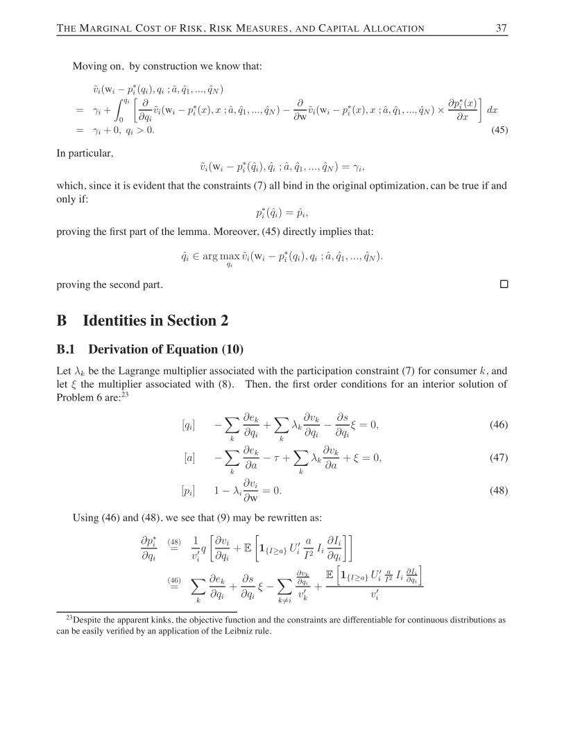
THE MARGINAL COST OF RISK, RISK MEASURES, AND CAPITAL ALLOCATION 37
Moving on, by construction we know that:
vi(wi & p#i (qi), qi ; a, q1, ..., qN )
= *i +
R qi
0
."
"qivi(wi & p#i (x), x ; a, q1, ..., qN )& "
"wvi(wi & p#i (x), x ; a, q1, ..., qN )$ "p#i (x)
"x
/dx
= *i + 0, qi > 0. (45)
In particular,vi(wi & p#i (qi), qi ; a, q1, ..., qN ) = #i,
which, since it is evident that the constraints (7) all bind in the original optimization, can be true if andonly if:
p#i (qi) = pi,
proving the first part of the lemma. Moreover, (45) directly implies that:
qi # argmaxqi
vi(wi & p#i (qi), qi ; a, q1, ..., qN).
proving the second part.
B Identities in Section 2
B.1 Derivation of Equation (10)Let /k be the Lagrange multiplier associated with the participation constraint (7) for consumer k, andlet 0 the multiplier associated with (8). Then, the first order conditions for an interior solution ofProblem 6 are:23
[qi] &!
k
$ek$qi
+!
k
/k$vk$qi
& $s
$qi0 = 0, (46)
[a] &!
k
$ek$a
& " +!
k
/k$vk$a
+ 0 = 0, (47)
[pi] 1& /i$vi$w
= 0. (48)
Using (46) and (48), we see that (9) may be rewritten as:
$p#i$qi
(48)=
1
v"iq
.$vi$qi
+ E.1{I!a} U
"i
a
I2Ii$Ii$qi
//
(46)=
!
k
$ek$qi
+$s
$qi0 &!
k )=i
!vk!qi
v"k+
E01{I!a} U "
iaI2 Ii
!Ii!qi
1
v"i
23Despite the apparent kinks, the objective function and the constraints are differentiable for continuous distributions ascan be easily verified by an application of the Leibniz rule.

THE MARGINAL COST OF RISK, RISK MEASURES, AND CAPITAL ALLOCATION 38
or, simplifying and using (47):
$p#i$qi
=$eZi$qi
+$s
$qi
+!
k
$ek$a
+ " &!
k
!vk!a
v"k
,+ E
+1{I!a}
!
k
U "k
v"k
a
I2Ik$Ii$qi
,.
Moving on:
$p#i$qi
=$eZi$qi
+$s
$qi
+P(I % a) + " &
!
k
!vk!a
v"k
,+
E01{I!a}
2k
U !k
v!k
1I2 Ik
!Ii!qi
1
2k
!vk!av!k
$!
k
!vk!a
v"k$ a
and, therefore, (10).
B.2 Derivation of Equation (18)In the setting of Section 2.2, the firm’s problem becomes:
maxa,{qi},{pi},{Kj},{wij}
!pi &
!ei & " a,
subject to:
vi % #i,
s(q1, . . . , qN) ( a,!
j
&j Kj = 1,
!
j
&j wij = wi.
In addition to a new set of optimality conditions connected with {Kj} and {wij}, we have the sameset of first order conditions:
[qi] &!
k
$ek$qi
+!
k
/k$vk$qi
& $s
$qi0 = 0,
[a] &!
k
$ek$a
& " +!
k
/k$vk$a
+ 0 = 0,
[pi] 1& /i$vi$w
= 0.
The first order condition for {wij} is:
[wij ] /i$vi$wij
& 1i &j = 0 (49)
1 /i p(S)j EP
0U "i(Wi & pi & Li +Ri)|!(S)
j
1& 1i &j = 0,

THE MARGINAL COST OF RISK, RISK MEASURES, AND CAPITAL ALLOCATION 39
where {1i} are the Lagrange multipliers for the individual wealth constraints. Since
0 =!
j
3/i p
(S)j EP
0U "i(Wi & pi & Li +Ri)|!(S)
j
1& 1i &j
4
= /i$vi$w
& 1i,
with [pi] we obtain 1i . 1. Thus, we also have:
&j
p(S)j
=EP0U "i(Wi & pi & Li +Ri)|!(S)
j
1
!vi!w
. (50)
As before, we seek a pricing function satisfying:.$vi$qi
+ EP.1{I!K a} U
"i
K a
I2Ii$Ii$qi
//& $vi$w
$p#i$qi
= 0.
Proceeding analogously to Appendix B.1, we arrive at the marginal pricing condition associated with adecentralized implementation:
$p#i$qi
=!
k
$ek$qi
+$s
$qi0 &!
k )=i
!vk!qi
v"k+
EP01{I!K a} U "
iK aI2 Ii
!Ii!qi
1
v"i.
Simplifying, we obtain:
"p#i"qi
="eZi"qi
+"s
"qi
+!
k
"ek"a
+ ! &!
k
!vk!a
v"k
,+ EP
+1{I!K a}
!
k
U "k
v"k
K a
I2Ik
"Ii"qi
,
="eZi"qi
+"s
"qi
+EQ $K 1{I!K a}
%+ ! &
!
k
!vk!a
v"k
,+
EP01{I!K a}
2k
U !k
v!k
KI2 Ik
!Ii!qi
1
2k
!vk!av!k
$!
k
!vk!a
v"k$ a
="eZi"qi
+"s
"qi
+
EQ $K 1{I!K a}%+ ! &
!
k
!vk!a
v"k
,
+ #i $ a$+!
k
!vk!a
v"k
,
,
i.e. (17), where:
%i =EP01{I!K a}
2k
U !k
v!k
KI2 Ik
!Ii!qi
1
EP01{I!K a}
2k
U !k
v!kK Ik
I
1 (50)=
EQ01{I!K a}
2k
U !k
EP[U !k|#(S)]
KI2 Ik
!Ii!qi
1
EQ01{I!K a}
2k
U !k
EP[U !k|#(S)]
K IkI
1 ,
i.e. (18). In the limiting case of a complete market, clearly U "i(wij & pi & lij + rij) is F (S)-measurable,
so that we immediately obtain (19).

THE MARGINAL COST OF RISK, RISK MEASURES, AND CAPITAL ALLOCATION 40
B.3 Derivation of Equation (24)The first order conditions of program (23) are:24
[qi] &!
k
$ek$qi
& V E.$Ii(Li, qi)
$qi
1{I=a}
dt
/+!
k
/k$vk$qi
& 0 $s$qi
= 0, (51)
[a] &!
k
$ek$a
& " +!
k
/k$vk$a
+ 0 + V fI(a) = 0, (52)
[pi] 1& /i$vi$w
= 0, (53)
where—as before—/i and 0 denote the Lagrange multipliers for the first set of conditions and thesecond condition, respectively, and fI denotes the cumulative density function of I .
Again, we assume each consumer is a “price taker” and ignores the impact of her own purchase atthe margin on the level of recoveries in states of default, so that the marginal price change at the optimallevel of qi must satisfy:
$vi$w
$p#i$qi
=$vi$qi
+ E.1{I>a}
a
(I)2Ii$Ii$qi
U "i
/.
Therefore:
$p#i$qi
=1!vi!w
.$vi$qi
+ E.1{I>a}
a
(I)2Ii$Ii$qi
U "i
//
=!
k
$ek$qi
+ 0$s
$qi+ V E
.$Ii(Li, qi)
$qi
1{I=a}
dt
/&!
k )=i
!vk!qi
v"k+
E01{I>a}
a(I)2 Ii
!Ii!qi
U "i
1
v"i
=$eZk$qi
+
+
P(I % a) + " &!
k
!vk!a
v"k& V fI(a)
,$s
$qi+ V fI(a)E
.$Ii$qi
8888 I = a
/
+E+
1{I>a}!
k
U "k
v"k
a
(I)2Ik$Ii$qi
,
and since:!
k
!vk!a
v"k= E
+1{I>a}
!
k
U "k
v"k
IkI
,,
we obtain (24).24For simplicity, we omit the “t” super- and subscripts in case no ambiguity arises.

THE MARGINAL COST OF RISK, RISK MEASURES, AND CAPITAL ALLOCATION 41
C Identities in Section 4
C.1 Derivation of Equation (34)For consumerN , LN / Exp(-) and the loss incurred by “the other” consumers is L%N =
2N%1i=1 Li /
Gamma(N & 1, -). Then
e = eN = E$q LN 1{q(L"N+LN )<a}
%& '( )
part i.
+ aE.
q LN
q (L%N + LN )1{q(L"N+LN )!a}
/
& '( )part ii.
.
For part ii., note that LNL"N+LN
is Beta(1, N&1) distributed independent of L%N+LN / Gamma(N, -).Hence, part ii. can be written as
aPCL%N + LN % a
q
DE.
LN
L%N + LN
/= a %N,)
Ca
q
DN%1.
For part i., we have
q E$LN 1{q(L"N+LN )<a}
%
= q
R &
0
R &
01{i+l<a/q} l ) e
%) l )N%1
(N & 2)!iN%2 e%) i dl di
= q)N
(N & 2)!
R a/q
0
R a/q%i
0le%) l dl iN%2 e%) i di
= q)N
(N & 2)!
R a/q
0
.1
)2& 1
)
Ca
q+
1
)
De%) a/q e) i + i
1
)e%) a/q e) i
/iN%2 e%) i di
= q)N%2
(N & 2)!
R a/q
0iN%2 e%) i di& q
)N%1
(N & 2)!e%) a/q
+Ca
q+
1
)
DR a/q
0iN%2 di&
R a/q
0iN%1 di
,
=q
)!N%1,)(a/q)& q
)N%1
(N & 1)!e%) a/q
Ca
q
DN%1 .1)+
1
N
a
q
/.
Therefore, since all consumers are identical, the objective function (6) takes the form displayed in (34).For condition (7), on the other hand, we have
V = VN = E [U (w& p& LN +RN )]
= E$U (w& p& (1& q)LN ) 1{q(L"N+LN )<a}
%& '( )
part i.
+E.U
Cw& p& LN + a
LN
L%N + LN
D1{q(L"N+LN )!a}
/
& '( )part ii.
For part i, we obtain
E$U (w & p& (1& q)LN ) 1{q(L"N+LN )<a}
%
= &R &
0
R &
01{i+l<a/q}e
%((w%p%(1%q)l) ) e%) l)N%1
(N & 2)!iN%2 e%) i dl di

THE MARGINAL COST OF RISK, RISK MEASURES, AND CAPITAL ALLOCATION 42
= &e%((w%p)R a/q
0
1
) & '(1 & q)
01& e%a/q()%(1%q)()%i(1%q))+i)
1 )N%1
(N & 2)!iN%2 e%) i di
= e%((w%p)
+1
) & '(1& q)!N%1,)(a/q)&
e%aq ()%(1%q)())N%1
((1& q)')N%1!N%1,(1%q)(
Ca
q
D,.
For part ii., note that
E.U
Cw& p& ((L%N + LN )& a)
LN
L%N + LN
D1{q(L"N+LN )!a}
/
=
R 1
0
R &
0e%((w%p%(l%a)y)1{l!a/q}
)N
(N & 1)!lN%1 e%) l (N & 1) (1 & y)N%2 dl dy
= &e%((w%p)R &
a/q
)N
(N & 1)!e%) l lN%1
R 1
0e(((l%a))y(N & 1) (1 & y)N%2 dy
& '( )mgfBeta(1,N"1)(((l%a))
dl
= &e%((w%p)R &
a/q
)N
(N & 1)!e%) l lN%1
&!
k=0
('(l & a))k
(N & 1 + k)!dl
= &e%((w%p)&!
k=0
N%1!
j=0
5N " 1
j
6aj e%) a
'k
(N & 1 + k)!
(N + k & j & 1)!
)%j+k
$R &
a/q
)N+k%j
(N + k & j & 1)!e%) (l%a) (l & a)N+k%j%1 dl
= &e%((w%p)&!
k=0
N%1!
j=0
(N & 1)!
(N & 1 + k)!
(a))j
j!e%) a
3')
4k (N + k & j & 1)!
(N & 1& j)!!N%j+k,)
Ca
C1& q
q
DD.
C.2 Derivation of Equation (36)Similar to the previous part, for consumer N with L =
2Ni=1 Li:
E+
N!
j=1
U "Cw& p& Lj + a
Lj
L
DLj
L
LN
L
88888L,
=N%1!
j=1
E.U "Cw& p& (L& a)
Lj
L
DLj
L
LN
L
8888L/
& '( )part i.
+E+U "Cw& p& (L& a)
LN
L
DCLN
L
D288888L,
& '( )part ii.
.
Note that Lj
L , LNL / Beta(1, N & 1) and for the joint distribution
fLjL ,
LNL
(x, y) = (1& x& y)N%3 (N & 2) (N & 1) 1{x,y!0,x+y'1}, j 0= N.
Whence, for part i.,
E.U "Cw& p& (L& a)
LN%1
L
DLN%1
L
LN
L
8888L/

THE MARGINAL COST OF RISK, RISK MEASURES, AND CAPITAL ALLOCATION 43
= + e%((w%p)
R 1
0
R 1%x
0
e((L%a)x x y (N & 1) (N & 2) (1& x& y)N%3 dy dx
= + e%((w%p)
R 1
0
e((L%a)xx
R 1%x
0
y (N & 1) (N & 2) (1& x& y)N%3 dy& '( )
=(1%x)N"1
dx
= + e%((w%p) 2(2, N)
R 1
0
e((L%a)x 1
2(2, N)x (1& x)N%1 dx
& '( )=mgfBeta(2,N)(((L%a))
= + e%((w%p) 1
N(N + 1)(N + 1)!
&!
k=0
(k + 1) (+(L& a))k
(N + k + 1)!,
whereas for part ii.,
E+U "Cw& p& (L& a)
LN
L
DCLN
L
D288888L,
= +e%((w%p) E+exp
;+(L& a)
LN
L
<CLN
L
D288888L,
& '( )= !2
!t2mgfBeta(1,N"1)(t)
"""t=$(L"a)
= + e%((w%p)(N & 1)!&!
k=0
(k + 1) (k + 2) (+(L& a))k
(N + k + 1)!,
so that
E+
N!
j=1
u"Cw & p& Lj + a
Lj
L
DLj
L
LN
L
88888L,
= + e%((w%p)(N & 1)!&!
k=0
(N & 1) (k + 1) (+(L& a))k + (k + 1) (k + 2) (+(L& a))k
(N + k + 1)!
= + e%((w%p)(N & 1)!&!
k=0
(k + 1) (N + 1 + k) (+(L& a))k
(N + k + 1)!
= + e%((w%p)(N & 1)!&!
k=0
(k + 1) (+(L& a))k
(N + k)!.
For the denominator,
E
=
?1{q L!a}
N!
j=1
U "Cw& p& Lj & a
Lj
L
DLj
L
@
B
= E+
1{q L!a} N ' e%((w%p) (N & 1)!&!
k=0
(k + 1) ('(L& a))k
(N + k)!
,

THE MARGINAL COST OF RISK, RISK MEASURES, AND CAPITAL ALLOCATION 44
= N !' e%((w%p)&!
k=0
k + 1
(N + k)!'kR &
a/q
)N
(N & 1)!(l & a)k lN%1 e%) l dl
= N !' e%((w%p)&!
k=0
3')
4k k + 1
(N + k)!e%) a
N%1!
j=0
5N " 1
j
6(a))j
(N + k & j & 1)!
(N & 1)!
$R &
a/q
)N+k%j
(N + k & j & 1)!e%)(l%a) (l & a)N+k%j%1 dl
= N !' e%((w%p)&!
k=0
3')
4k k + 1
(N + k)!e%) a
N%1!
j=0
(a))j
j!
(N + k & j & 1)!
(N & j & 1)!!N+k%j,)
Ca
C1& q
q
DD.
Hence,
q #i =1
NE
=
>>>>>>?1{q L!a}
2&k=0
(k+1) (((L%a))k
(N+k)!2&
k=0
5()
6k k+1(N+k)! e
%) a2N%1j=0
(a))j
j!(N+k%j%1)!(N%j%1)! !N+k%j,)
3a31%qq
44
& '( )=*(L)
@
AAAAAAB.
For implementation purposes, the numerator can be expressed as&!
k=0
(k + 1) tk
(N + k)!
88888t=((L%a)
="
"t
+ &!
k=0
tk+1
(N + k)!
,88888t=((L%a)
="
"t
+
t%(N%1)&!
k=N
tk
k!
,88888t=((L%a)
="
"t
+t%(N%1)
*et &
N%1!
k=0
tk
k!
-,88888t=((L%a)
= &(N & 1)t%N
*
et &N%1!
k=0
tk
k!
-
+ t%(N%1)
*
et &N%1!
k=0
k tk%1
k!
-88888t=((L%a)
=
*et &
N%2!
k=0
tk
k!
-$5t%N+1 & t%N (N & 1)
6+
(N & 1)
(N & 1)!t%1
88888t=((L%a)
.
Finally,
.(I) = .(qL) = E+$PP
88888L
,
= const E+
N!
j=1
+ exp
;&+Cw& p& Lj + a
Lj
L
D<Lj
L
88888L,
= const N E.e((L%a)Lj/L
Lj
L
8888L/
= const $
$xmgfBeta(1,N%1)(x)
8888x=((L%a)
= .(L),
since E0.(I)
1= 1.

THE MARGINAL COST OF RISK, RISK MEASURES, AND CAPITAL ALLOCATION 45
References
Acerbi, C. (2002). “Spectral Measures of Risk: A Coherent Representation of Subjective Risk Aver-
sion.” Journal of Banking and Finance 26, 1505-1518.
Adrian, T., and Shin, H. (2008). “Financial Intermediary Leverage and Value-at-Risk.” Federal Reserve
Bank of New York Staff Report 338.
Artzner, P., Delbaen, F., Eber, J.M., and Heath, D. (1999). “Coherent Measures of Risk.” Mathematical
Finance 9, 203-228.
Basak, S., and Chabakauri, S. (2006). “DynamicMean-Variance Asset Allocation.” Review of Financial
Studies 23: 2970-3016.
Bjork, T., and Slinko, I. (2006). “Towards a General Theory of Good-Deal Bounds.” Review of Fi-
nance 10: 221-260.
Cerny, A. (2003). “Generalised Sharpe Ratios and Asset Pricing in Incomplete Markets.” Review of
Finance 7: 191-233.
Denault, M. (2001). “Coherent Allocation of Risk Capital.” Journal of Risk 4, 7-21.
Detlefsen, K., and Scandolo, G. (2005). “Conditional and dynamic convex risk measures.” Finance
and Stochastics 9, 539-561.
Dhaene, J., Laeven, R.J.A., Vanduffel, S., Darkiewicz, G., and Goovaerts, M. J. (2008). “Can a Coher-
ent Risk Measure be too Subadditive?” Journal of Risk and Insurance 75, 365-386.
Follmer, H., and Schied, A. (2002). “Convex measures of risk and trading constraints.” Finance and
Stochastics 6, 429-447.
Follmer, H., and Schied, A. (2010). “Coherent and Convex Risk Measures.” In Encyclopedia of
Quantitative Finance, Cont, R. (Ed.), Wiley, 355-363.
Follmer, H., and Schweizer, M. (2010). “Minimal Martingale Measure.” In Encyclopedia of Quantita-
tive Finance, Cont, R. (Ed.), Wiley, 1200-1204.

THE MARGINAL COST OF RISK, RISK MEASURES, AND CAPITAL ALLOCATION 46
Frittelli, M., Gianin, E.R. (2002). “Putting Order in Risk Measures.” Journal of Banking and Fi-
nance 26, 1473-1486.
Froot, K.A. (2007). “Risk Management, Capital Budgeting, and Capital Structure Policy for Insurers
and Reinsurers.” Journal of Risk and Insurance 74, 273-299.
Froot, K.A., Scharfstein, D.S., and Stein, J.C. (1993). “Risk Management: Coordinating Corporate
Investment and Financing Policies.” Journal of Finance 48, 1629-1658.
Froot, K.A., and Stein, J. (1998). “Risk Management, Capital Budgeting, and Capital Structure Policy
for Financial Institutions: An Integrated Approach.” Journal of Financial Economics 47, 55-82.
Goll, T., and Ruschendorf, L. (2001). “Minimax and minimal distance martingale measures and their
relationship to portfolio optimization.” Finance and Stochastics 5: 557-581.
Gourieroux, C., Laurent, J.P., and Scaillet, O. (2000). “Sensitivity analysis of Values at Risk.” Journal
of Empirical Finance 7, 225-245.
Grundl, H., and H. Schmeiser (2007). “Capital Allocation for Insurance Companies: What Good Is
It?” Journal of Risk and Insurance 74, 301-317.
Hanif, F., Hocking, J., Jaekel, A., and Ziewer, L. (2010). “Solvency 2: Quantitative & Strategic Impact
– The Tide is Going Out.” Morgan Stanley and Oliver Wyman Blue Paper.
Henderson, V., Hobson, D., Howinson, S., and Kluge, T. (2005). “A Comparison of Option Prices
Under Different Pricing Measures in a Stochastic Volatility Model with Correlation.” Review of
Derivatives Research 8: 5-25.
Hull, J. (2007) “VAR versus Expected Shortfall.” Risk Magazine, March 2007.
Ibragimov, R., Jaffee, D., and Walden, J., (2010) “Pricing and Capital Allocation for Multiline Insur-
ance Firms.” Journal of Risk and Insurance 77, 551-578.
International Actuarial Association (2004). “A Global Framework for Insurer Solvency As-
sessment.” IAA Insurer Solvency Assessment Working Party Research Report. Availabe

THE MARGINAL COST OF RISK, RISK MEASURES, AND CAPITAL ALLOCATION 47
at http://www.actuaries.org/LIBRARY/Papers/Global_Framework_Insurer_
Solvency_Assessment-public.pdf.
Kalkbrener, M. (2005). “An Axiomatic Approach to Capital Allocation.” Mathematical Finance 15,
425-37.
Keeler, T.E., and Small, K.A. (1977). “Optimal Peak Load Pricing, Investment, and Service Levels on
Urban Expressways.” Journal of Political Economy 85, 1-25.
Kou, S.G., Peng, X.H., and Heyde, C.C., (2012). “External Risk Measures and Basel Accords.” Math-
ematics of Operations Research, forthcoming.
McKinsey&Company (2011). “The use of economic capital in performance management for banks:
A perspective.” Prepared by T. Baer, A. Mehta, and H. Samandari. McKinsey Working Papers on
Risk, Number 24. Availabe at http://www.mckinsey.com/clientservice/risk/pdf/
risk_working_papers/24_The_Use_of_Economic_Capital.pdf.
McNeil, A.J., Frey, R., and Embrechts, P. (2005). “Quantitative Risk Management: Concepts, Tech-
niques, and Tools.” Princeton: Princeton University Press.
Myers, S.C., and Read, J.A. (2001). “Capital Allocation for Insurance Companies.” Journal of Risk
and Insurance 68, 545-80.
National Association of Insurance Commissioners (NAIC) (2009). “Consultation Paper on Regulatory
Capital Requirements and Overarching Accounting/Valuation Issues for the SolvencyModernization
Initiative.” Availabe at http://www.naic.org/documents/committees_ex_isftf_
iswg_capital_requirements.doc.
Phillips, R.D., Cummins, J.D., and Allen, F. (1998). “Finanical Pricing of Insurance in the Multiple
Line Insurance Company.” Journal of Risk and Insurance 65, 597-636.
Powers, M.R. (2007). “Using Aumann-Shapley Values to Allocate Insurance Risk: The Case of Inho-
mogeneous Losses.” North American Actuarial Journal 11, 113-27.

THE MARGINAL COST OF RISK, RISK MEASURES, AND CAPITAL ALLOCATION 48
Schmock, U., and Straumann, D. (1999). “Allocation of Risk Capital and Performance Measurement.”
Presentation at the Risk Day 1999, Zurich. Available at http://www.fam.tuwien.ac.at/
˜schmock/slides/AllocationSlidesOct1999.pdf.
Smith, C.W., Smithson, C.W., and Wilford, S.D. (1990). “Managing Financial Risk.” New York, NY,
Harper Business, 355-378.
Smith, C.W., and Stulz, R.M. (1985). “The Determinants of Firms Hedging Policies.” Journal of
Financial and Quantitative Analysis 20, 391-405.
Society of Actuaries (2008). “Economic Capital for Life Insurance Companies.” Research report
prepared by I. Farr, H. Mueller, M. Scanlon, and S. Stronkhorst. Availabe at http://www.soa.
org/files/pdf/research-ec-report.pdf.
Stoughton, N.M., and Zechner, J. (2007). “Optimal Capital Allocation Using RAROC and EVA.”
Journal of Financial Intermediation 16, 312-342.
Tasche, D. (2004). “Allocating Portfolio Economic Capital to Sub-portfolios.” In: Economic Capital:
A Practitioner Guide, A. Dev (ed.). Risk Books, 2004, 275-302.
Zanjani, G. (2002). “Pricing and Capital Allocation in Catastrophe Insurance.” Journal of Financial
Economics 65, 283-305.
Zanjani, G. (2010). “An Economic Approach to Capital Allocation.” Journal of Risk and Insurance 77,
523-549.