HAL Id: tel-01677743https://tel.archives-ouvertes.fr/tel-01677743

Submitted on 8 Jan 2018

HAL is a multi-disciplinary open accessarchive for the deposit and dissemination of sci-entific research documents, whether they are pub-lished or not. The documents may come fromteaching and research institutions in France orabroad, or from public or private research centers.

L’archive ouverte pluridisciplinaire HAL, estdestinée au dépôt et à la diffusion de documentsscientifiques de niveau recherche, publiés ou non,émanant des établissements d’enseignement et derecherche français ou étrangers, des laboratoirespublics ou privés.

The management of multiple submissions in parallelsystems : the fair scheduling approach

Vinicius Gama Pinheiro

To cite this version:Vinicius Gama Pinheiro. The management of multiple submissions in parallel systems : the fairscheduling approach. Symbolic Computation [cs.SC]. Université de Grenoble; Universidade de SãoPaulo (Brésil), 2014. English. �NNT : 2014GRENM042�. �tel-01677743�

THÈSEPour obtenir le grade de

DOCTEUR DE L’UNIVERSITÉ DE GRENOBLESpécialité : Mathématiques-informatique

Arrêté ministérial : 7 août 2006

Présentée par

Vinicius Gama Pinheiro

Thèse dirigée par Denis Trystramet codirigée par Alfredo Goldman

préparée au sein LIG, Laboratoire d’Informatique de Grenobleet de École Doctorale Mathématiques, Sciences et Technologies del’Information, Informatique

The management of multiple sub-missions in parallel systems: thefair scheduling approach

Thèse soutenue publiquement le 14 février 2013,devant le jury composé de :

Alfredo GoldmanProfesseur des universités, Universidade de São Paulo, Brasil, PrésidentEvripidis BampisProfesseur des universités, Université Pierre et Marie Curie, France, RapporteurEdmundo MadeiraProfessor titular, Universidade de Campinas, Brasil, RapporteurFrédéric SuterChercheur, CNRS, Institut National de Physique Nucléaire et de Physique desParticules, France, ExaminateurLuiz BittencourtProfessor Assistente, Universidade de Campinas, Brasil, ExaminateurDenis TrystramProfesseur des universités, Grenoble Institute of Technology, France, Directeurde thèseAlfredo GoldmanProfessor Associado, Universidade de São Paulo, Brasil, Co-Directeur de thèse

For Cécile Zozzoli, a true life partner, a beautiful woman, and a loving wifewhose affection, comprehension, and devotion inspire me and bring joy to my life.

Acknowledgements

This thesis represents not only a technical piece of work but also a personal overcom-ing, given the challenges that appeared on my way, some anticipated, others completelyunexpected. Many people contributed for my success in this endeavor.

First, I would like to thank Prof. Denis Trystram for being my advisor, specially duringmy stay in France. I am very grateful for all the guidance he provided me during my studies,for his patience, and also for receiving me so well in your research group.

To my Brazilian advisor, Prof. Alfredo Goldman, thank you for all the support, friendshipand patience. And for always trusting me.

To Prof. Krzysztof Rzadca, from University of Warsaw, thank you for the great discussionsand academic partnership in writing papers. Oh, and thank you for having lent me yourbike! I really enjoyed the time I spent in Warsaw.

Another professors also helped me along the way: Prof. Arnaud Legrand, Prof. DanielCordeiro, and Prof. Daniel Batista. Thank you all for the fruitful discussions and suggestions.

To my LIG mates Emílio Francesquini, Marcio Castro, and Gabriel Duarte: my stay inFrance was way more pleasant beside you guys. Also, a big thank you for Valentin Reis andJoseph Emeras, great study partners.

To my LCPD mates Paulo Meirelles, Gustavo Duarte, Raphael Cobe, Beraldo Leal, andMarcio Vinicius: thank you for the great moments in the lab and on the campus.

Last, but not least important, to Cécile Zozzoli, my dear wife, and to Getúlio, Marilene,Rúbia and Jacqueline Pinheiro, my parents and sisters, beloved ones.

iii

Abstract

The High Performance Computing community is constantly facing new challengesdue to the ever growing demand for processing power from scientific applications thatrepresent diverse areas of human knowledge. Parallel and distributed systems are the keyto speed up the execution of these applications as many jobs can be executed concurrently.These systems are shared by many users who submit their jobs over time and expect a fairtreatment by the scheduler.

The work done in this thesis lies in this context: to analyze and develop fair and efficientalgorithms for managing computing resources shared among multiple users. We analyzescenarios with many submissions issued from multiple users over time. These submissionscontain several jobs and the set of submissions are organized in successive campaigns. Inwhat we define as the Campaign Scheduling model, the jobs of a campaign do not startuntil all the jobs from the previous campaign are completed. Each user is interested inminimizing the sum of the campaigns‘ flow times. This is motivated by the user submissionbehavior whereas the execution of a new campaign can be tuned by the results of theprevious campaign.

In the first part of this work, we define a theoretical model for Campaign Schedulingunder restrictive assumptions and we show that, in the general case, it is NP-hard. For thesingle-user case, we show that an approximation scheduling algorithm for the (classic)parallel job scheduling problem also delivers the same approximation ratio for the CampaignScheduling problem. For the general case with multiple users, we establish a fairness criteriainspired by time sharing. Then, we propose a scheduling algorithm called FairCamp whichuses campaign deadlines to achieve fairness among users between consecutive campaigns.

The second part of this work explores a more relaxed and realistic Campaign Schedulingmodel, provided with dynamic features. To handle this setting, we propose a new algorithmcalled OStrich whose principle is to maintain a virtual time-sharing schedule in which thesame amount of processors is assigned to each user. The completion times in the virtualschedule determine the execution order on the physical processors. Then, the campaigns areinterleaved in a fair way. For independent sequential jobs, we show that OStrich guaranteesthe stretch of a campaign to be proportional to campaign’s size and to the total numberof users. The stretch is used for measuring by what factor a workload is slowed downrelatively to the time it takes to be executed on an unloaded system.

Finally, the third part of this work extends the capabilities of OStrich to handle paralleljobs. This new version executes campaigns using a greedy approach and uses an event-based resizing mechanism to shape the virtual time-sharing schedule according to thesystem utilization ratio.

Keywords: campaign, multi-user, fairness, scheduler

v

Résumé

La communauté de Calcul Haute Performance est constamment confrontée à de nou-veaux défis en raison de la demande toujours croissante de la puissance de traitementprovenant d’applications scientifiques diverses. Les systèmes parallèles et distribués sontla clé pour accélérer l’exécution de ces applications, et atteindre les défis associés car denombreux processus peuvent être exécutés simultanément. Ces systèmes sont partagés parde nombreux utilisateurs qui soumettent des tâches sur de longues périodes au fil du tempset qui attendent un traitement équitable par l’ordonnanceur.

Le travail effectué dans cette thèse se situe dans ce contexte: analyser et développer desalgorithmes équitables et efficaces pour la gestion des ressources informatiques partagésentre plusieurs utilisateurs. Nous analysons les scénarios avec de nombreux soumissionsissues de plusieurs utilisateurs. Ces soumissions contiennent un ou plusieurs processus etl’ensemble des soumissions sont organisées dans des campagnes successives. Dans ce quenous appelons le modèle d’ordonnancement des campagnes les processus d’une campagnene commencent pas avant que tous les processus de la campagne précédente soient ter-minés. Chaque utilisateur est intéressé à minimiser la somme des temps d’exécution deses campagnes. Cela est motivé par le comportement de l’utilisateur tandis que l’exécutiond’une campagne peut être réglé par les résultats de la campagne précédente.

Dans la première partie de ce travail, nous définissons un modèle théorique pourl’ordonnancement des campagnes sous des hypothèses restrictives et nous montrons que,dans le cas général, il est NP-difficile. Pour le cas mono-utilisateur, nous montrons quel’algorithme d’approximation pour le problème (classique) d’ordonnancement de processusparallèles fournit également le même rapport d’approximation pour l’ordonnancementdes campagnes. Pour le cas général avec plusieurs utilisateurs, nous établissons un critèred’équité inspiré par une situation idéalisée de partage des ressources. Ensuite, nous pro-posons un algorithme d’ordonnancement appelé FairCamp qui impose des dates limite pourles campagnes pour assurer l’équité entre les utilisateurs entre les campagnes successives.

La deuxième partie de ce travail explore un modèle d’ordonnancement de campagnesplus relâché et réaliste, avec des caractéristiques dynamiques. Pour gérer ce cadre, nousproposons un nouveau algorithme appelé OStrich dont le principe est de maintenir unordonnancement partagé virtuel dans lequel le même nombre de processeurs est assigné àchaque utilisateur. Les temps d’achèvement dans l’ordonnancement virtuel déterminentl’ordre d’exécution sur le processeurs physiques. Ensuite, les campagnes sont entrelacées demanière équitable. Pour des travaux indépendants séquentiels, nous montrons que OStrichgarantit le stretch d’une campagne en étant proportionnel à la taille de la campagne et lenombre total d’utilisateurs. Le stretch est utilisé pour mesurer le ralentissement par rapportau temps qu’il prendrait dans un système dédié.

Enfin, la troisième partie de ce travail étend les capacités d’OStrich pour gérer des tâches

vii

parallèles rigides. Cette nouvelle version exécute les campagnes utilisant une approchegourmande et se sert aussi d’un mécanisme de redimensionnement basé sur les événementspour mettre à jour l’ordonnancement virtuel selon le ratio d’utilisation du système.

Mots-clés: campaigne, multi-utilisateur, fairness, ordonnanceur.

Contents

List of Figures xi

1 Introduction 11.1 Fairness matters . . . . . . . . . . . . . . . . . . . . . . . . . . . . . . . . . . 31.2 Multiple submissions as job campaigns . . . . . . . . . . . . . . . . . . . . . 51.3 Thesis outline and contributions . . . . . . . . . . . . . . . . . . . . . . . . . 7

2 Background 92.1 Classical scheduling theory . . . . . . . . . . . . . . . . . . . . . . . . . . . 102.2 Single-objective scheduling . . . . . . . . . . . . . . . . . . . . . . . . . . . 112.3 Multi-objective scheduling . . . . . . . . . . . . . . . . . . . . . . . . . . . . 152.4 Fairness in scheduling . . . . . . . . . . . . . . . . . . . . . . . . . . . . . . 21

3 The Campaign Scheduling Problem 313.1 The campaign model . . . . . . . . . . . . . . . . . . . . . . . . . . . . . . . 323.2 Related models . . . . . . . . . . . . . . . . . . . . . . . . . . . . . . . . . . 32

3.2.1 Bag-of-Tasks . . . . . . . . . . . . . . . . . . . . . . . . . . . . . . . . 333.2.2 Parameter sweep applications. . . . . . . . . . . . . . . . . . . . . . . 333.2.3 BSP model. . . . . . . . . . . . . . . . . . . . . . . . . . . . . . . . . 333.2.4 Similarities and applicability . . . . . . . . . . . . . . . . . . . . . . . 34

3.3 Definitions and notation . . . . . . . . . . . . . . . . . . . . . . . . . . . . . 353.4 Offline scheduling of single user’s campaigns . . . . . . . . . . . . . . . . . . 383.5 Offline scheduling with multiple users . . . . . . . . . . . . . . . . . . . . . 413.6 Online scheduling with multiple users . . . . . . . . . . . . . . . . . . . . . 43

3.6.1 Measuring fairness by max-stretch . . . . . . . . . . . . . . . . . . . 433.6.2 FCFS in multi-user systems . . . . . . . . . . . . . . . . . . . . . . . 44

4 Fair online schedules: constrained scenario 474.1 The FairCamp online algorithm . . . . . . . . . . . . . . . . . . . . . . . . . 484.2 Example . . . . . . . . . . . . . . . . . . . . . . . . . . . . . . . . . . . . . . 484.3 Algorithm description . . . . . . . . . . . . . . . . . . . . . . . . . . . . . . 494.4 Feasibility of FairCamp . . . . . . . . . . . . . . . . . . . . . . . . . . . . . . 514.5 Theoretical analysis . . . . . . . . . . . . . . . . . . . . . . . . . . . . . . . . 524.6 Simulations . . . . . . . . . . . . . . . . . . . . . . . . . . . . . . . . . . . . 54

ix

5 Fair online schedules: dynamic scenario 575.1 The OStrich online algorithm . . . . . . . . . . . . . . . . . . . . . . . . . . 585.2 Example . . . . . . . . . . . . . . . . . . . . . . . . . . . . . . . . . . . . . . 605.3 Theoretical analysis . . . . . . . . . . . . . . . . . . . . . . . . . . . . . . . . 63

5.3.1 Worst-case bound . . . . . . . . . . . . . . . . . . . . . . . . . . . . . 635.3.2 Tightness . . . . . . . . . . . . . . . . . . . . . . . . . . . . . . . . . 67

5.4 Analysis of campaigns in workloads . . . . . . . . . . . . . . . . . . . . . . . 675.4.1 Workload modeling . . . . . . . . . . . . . . . . . . . . . . . . . . . . 685.4.2 Example . . . . . . . . . . . . . . . . . . . . . . . . . . . . . . . . . . 695.4.3 Interval graphs for job dependencies . . . . . . . . . . . . . . . . . . 705.4.4 Campaigns with dependencies: a formal model . . . . . . . . . . . . 71

5.5 Simulations . . . . . . . . . . . . . . . . . . . . . . . . . . . . . . . . . . . . 71

6 Scheduling parallel jobs with OStrich 796.1 Parallel OStrich . . . . . . . . . . . . . . . . . . . . . . . . . . . . . . . . . . 79

6.1.1 Event based resizing . . . . . . . . . . . . . . . . . . . . . . . . . . . 806.2 Algorithm description . . . . . . . . . . . . . . . . . . . . . . . . . . . . . . 826.3 Example . . . . . . . . . . . . . . . . . . . . . . . . . . . . . . . . . . . . . . 836.4 Comparison with existing scheduling strategies . . . . . . . . . . . . . . . . 846.5 Theoretical analysis . . . . . . . . . . . . . . . . . . . . . . . . . . . . . . . . 87

6.5.1 Worst-case bound . . . . . . . . . . . . . . . . . . . . . . . . . . . . . 88

7 Conclusion and ongoing work 917.1 Work contributions and perspectives . . . . . . . . . . . . . . . . . . . . . . 92

Bibliography 95

List of Figures

1.1 Campaign Scheduling with 2 users (user 1 in light gray, user 2 in dark gray) 6

2.1 Example of a Gantt chart with 3 machines and 7 jobs . . . . . . . . . . . . . 102.2 List scheduling example with independent jobs . . . . . . . . . . . . . . . . 132.3 LPT Gantt charts . . . . . . . . . . . . . . . . . . . . . . . . . . . . . . . . . 142.4 Pareto set for the set of solutions X = {X1, X2} . . . . . . . . . . . . . . . . 172.5 Approximability bound for MUSP . . . . . . . . . . . . . . . . . . . . . . . . 182.6 Pareto optimality for MUSP (user 1 in light gray, user 2 in dark gray) . . . . 202.7 Space-sharing schedule example with 3 users . . . . . . . . . . . . . . . . . 222.8 Time-sharing schedule example with 3 users . . . . . . . . . . . . . . . . . . 222.9 Examples of space-share and time-share schedules with 2 users and corre-

sponding Pareto solutions . . . . . . . . . . . . . . . . . . . . . . . . . . . . 232.10 FCFS worst-case ratio with 2 users . . . . . . . . . . . . . . . . . . . . . . . 252.11 LPT starvation with 2 users . . . . . . . . . . . . . . . . . . . . . . . . . . . 262.12 SPT starvation with 2 users . . . . . . . . . . . . . . . . . . . . . . . . . . . 262.13 Example of Hadoop Fair Scheduler pools with 3 users . . . . . . . . . . . . . 282.14 Example of Slurm schedule with 3 users using Fair-share factor and ∆t = 2 . 29

3.1 Campaign submission and execution on a 4 processor system . . . . . . . . 323.2 Campaign Scheduling with 2 users (user 1 in light gray, user 2 in dark gray) 363.3 FCFS competitiveness. k = 2, σ = 2, user 1 in light gray, user 2 in dark

gray. Max-stretch is (2p+ 2)/2 ≈ p (for large p); the optimal max-stretch is(2p+ 2)/(2p) ≈ 1 (for large p). The faded campaign represents the optimalposition of the second campaign for user 2. . . . . . . . . . . . . . . . . . . 45

4.1 Deadlines with k = 2 and multiple campaigns . . . . . . . . . . . . . . . . . 484.2 Example of schedule constructed by FairCamp (user 1 in light grey and user

2 in dark grey) . . . . . . . . . . . . . . . . . . . . . . . . . . . . . . . . . . 494.3 FCFS vs FairCamp; each point is an average over 103 instances; error bars

denote 95% confidence intervals . . . . . . . . . . . . . . . . . . . . . . . . 544.4 Max-stretch distribution for FCFS and FairCamp with 20 users . . . . . . . . 55

5.1 An example of the virtual and real schedule generated by the OStrich algo-rithm with 3 users . . . . . . . . . . . . . . . . . . . . . . . . . . . . . . . . 61

5.2 Analysis of OStrich: bound for the campaign stretch . . . . . . . . . . . . . . 655.3 An example of a campaign with seven jobs according to the MAX algorithm 705.4 A Directed Acyclic Graph (DAG) illustrating dependencies inside the cam-

paign (same campaign of Figure 5.3) . . . . . . . . . . . . . . . . . . . . . . 70

xi

5.5 Campaign stretch values distribution (original log: Maui, FCFS) . . . . . . . 735.6 Campaign stretch values distribution (OStrich) . . . . . . . . . . . . . . . . 745.7 System resources utilization for whole trace (original log: Maui, FCFS) . . . 745.8 System resources utilization for the whole trace (OStrich) . . . . . . . . . . 755.9 System resources utilization for the extract (original log: Maui, FCFS) . . . . 755.10 System resources utilization for the extract (OStrich, with job dependencies) 765.11 System resources utilization for the extract (OStrich, no dependencies) . . 765.12 Ostrich vs FCFS: stretch values by intervals . . . . . . . . . . . . . . . . . . . 775.13 Ostrich vs FCFS: max campaign stretch mean per user profile . . . . . . . . 78

6.1 Delay problem between real and virtual schedule . . . . . . . . . . . . . . . 806.2 Delay correction using a resized virtual schedule . . . . . . . . . . . . . . . 816.3 Virtual and real schedule generated by the OStrich algorithm with 3 users . 846.4 FCFS example with 2 users . . . . . . . . . . . . . . . . . . . . . . . . . . . 856.5 Space share example with 2 users . . . . . . . . . . . . . . . . . . . . . . . . 866.6 OStrich example with 2 users . . . . . . . . . . . . . . . . . . . . . . . . . . 876.7 Analysis of OStrich with parallel jobs: stretch bound of a campaign execution 90

“Equals should be treated equally

and unequals unequally – but in

proportion to their relevant

similarities and differences.”

Someone on Aristotle’s thoughtsChapter 1

Introduction

Since the second half of the last century, the hardware and software industries conducted

several technological advances that helped to enlarge the boundaries of computer science in

a wide variety of fields such as structural analysis, oil exploration, atmospheric simulation,

weather forecast, seismic data processing, defense applications, chemistry and genetic

analysis [ER06]. The emergence and popularization of parallel computing was one of the

major factors that contributed to this phenomena.

Parallelism is a concept that arose on the early days of computer science as a way for

speeding up the execution time of processes. It embraces a large variety of techniques used

to split jobs in several parts to be computed by interconnected processor units. It became

very popular during the eighties due to the appearance of the first commercially available

general purpose parallel machines. However, they were expensive machines and not easily

accessible [BTEP00]. The arrival of powerful microprocessors used in workstations provided

high computation power at reasonable costs and was a major factor for the emergence of

parallel high performance computers and systems like clusters, grids, supercomputers and

desktop grids. Currently, HPC systems with a cluster architecture represent more than 83%

of the systems on the list of the 500 most powerful systems in the world [Sit] 1.

Nevertheless, despite the fact that High Performance Computing systems (HPC systems)

are cheaper and easier to obtain than before, they are hosted by organizations rather1From the time of this writing, this list was last updated in June 2013.

1

1.0

than individuals. They require specialized personnel and robust infrastructures whose

management is complex and time consuming. Hence, these systems are commonly shared

by many users and projects who compete for the usage of the resources in order to execute

their jobs.

Typically, the management of resources is handled by local and distributed resource

managers through a consensual scheduling policy. Even with all the popularity achieved

by HPC systems, and the computational power they aggregate, scheduling management

remains one of the main challenges due to the complexity of the majority of scheduling

problems [BK]. It becomes even more complex if users desire fairness and performance

guarantees. The management of umbrella projects in BOINC platform is a good example

where these issues show their pertinence.

BOINC [And04] is a platform for volunteer computing, through which volunteers can

donate their machines’ CPU idle time to scientific projects. It comprises over 580, 000 hosts

that deliver more than 2, 300 TeraFLOP per day to several projects. BOINC projects usually

have hundreds of thousands of CPU-bound jobs. These projects are traditionally interested

in overall throughput, i.e., maximize the total number of jobs completed per day. Generally,

the jobs submitted through BOINC are independent and preemptive.

Each project has its own server which is responsible for distributing work units to clients

as well as recovering and validating results. But the tasks of deploying and maintaining a

BOINC server can represent a great burden in terms of time and money. Umbrella projects

appeared as a way to address this problem. Those are multi-user projects that share the

same infrastructure, each one hosting their scientific sub project. Besides the economy

advantage, this solution provides a much larger number of volunteers to every project than

if they had deployed their own server. But this solution also creates new challenges.

In such umbrella projects, it is common that the demand for computing power exceeds

the available supply, therefore a mechanism to split the supply among users is needed.

Nevertheless, each sub project has its own goals and distinct processing needs that can be

represented by objective functions. In the past, most users were throughput-oriented but

popularization of those systems attracted other types of users. Nowadays, response-time

1.1

users are increasingly common [DLG11]. Their jobs are divided into successive batches

of independent jobs released sequentially over time. For such users, throughput is not

meaningful as they are more interested in minimizing the time each campaign takes to be

executed.

In this thesis, we study how to improve fairness between response-time users in parallel

systems. We model variants of this problem according to different user submission dynamics

and job constraints. We provide solutions to each case and, using theoretical tools, we study

how the trade-off between fairness and user performance is met.

1.1 Fairness matters

Users are human beings and, as such, they are sensitive to the way resources are shared

in their social circles. The equity theory developed in 1965 by John Stacey Adams in

his seminal article entitled “Inequity in Social Exchange” [Ada65], argues that, in social

settings, individuals (e.g. users) are selfish in general, meaning that they look only for their

own objectives and reject the idea of not being treated fairly when compared to the other

individuals. According to this work, inequity exists between two persons A and B when

there is a difference between the ratio of A’s outcomes to A’s inputs and the ratio of B’s

outcomes to B’s inputs. This may happen in a direct exchange relationship between them

or when both are in an indirect exchange relationship with a third party and one compares

himself to the other.

This theory is mainly based on two concepts relating to the perception of justice and

injustice. The first one, called “relative deprivation” is a sociological concept developed by

Stouffer et al. [SLL+49] from his survey over American soldiers during World War II. The

authors observed that more educated soldiers were less satisfied with their status than less

educated ones, despite the fact that the former had better career opportunities in the army.

This paradox was explained by assuming that better-educated men, who had made more

investments in their formation, had higher levels of aspiration and, therefore, that they

were relatively deprived of status based on what they achieved. In short, this concept states

that the degree of satisfaction of one person is closely related to his/her expectations.

1.1

The second one, called distributive justice, is roughly defined as the perceived fairness

in the way costs and rewards are shared within a group. More formally, distributive justice

is achieved between two group members when:

A’s rewards - A’s costsA’s investments = B’s rewards - B’s costs

B’s investments

In other words, this concepts states that the justice perceived by an individual is not

only measured by his/her own ratio of profits to investments but, more importantly, the

relation between ratios within a group. Some members can feel unfairly treated if they

perceived that their ratio of profits is smaller than the other, even if it corresponds to their

expectations.

Relative deprivation and/or lack of distributive justice are also applied to users sharing

the resources of a system. They form a group with conflicting interests in an indirect

exchange relationship with a third party, in this case, the scheduler. The decisions taken by

the scheduler impact on the level of satisfaction experienced by each user. They will likely

to compare their “rewards” or, more appropriately to this domain, resource allocations (e.g.

processing share, allocated memory, etc.) to those of another and become envy of others

anytime they feel deprecated.

Ideally, users should not envy their counterparts in a shared system. The notion of

“envy-freeness” appeared in the book “Puzzle-Math” (1958) [GS58] from the physicists

Gamow and Stern. For an algorithm to be envy-free, each user must prefer to keep their

own allocations to swapping with other users.

Fair division of resources is also discussed in a very recent article by Procaccia entitled

“Cake Cutting: Not Just Child’s Play” [Pro13] where the author invites the computer

scientists to dwell on this problem. This article surveys several cake cutting algorithms

supporting that they can give insights that can be applied on the allocation of computational

resources. It also discuss the notion of “envy-freeness” [GS58] and how it is addressed by

existing theoretical models. However, it is very important to stress that, unlike what will

be seen in this thesis, these actual models do not encompass dynamic features like users

joining or leaving the system and online submissions.

Some of the concepts presented on this section will be adapted in the next chapter

1.2

when discussing about fair division for scheduling tasks from multiple users. On the next

section, it is presented the exchange nature (i.e. the interactive process) between users and

scheduler that drives all the analysis present on this thesis.

1.2 Multiple submissions as job campaigns

In this thesis, the problem of multiple submissions on parallel system is narrowed to the

notion of Campaign Scheduling. The campaign scheduling problem models a submission

pattern typically found in parallel systems used for scientific research: the user submits a

set of jobs, analyzes the outcomes and then resubmits another set of jobs [ZAT05, ZF12]. In

other words, the campaigns are sets of jobs issued from a user and they must be scheduled

one after the other since the submission of a new campaign depends on the outcome of the

previous one. Reflecting that, the maximum number of campaigns being simultaneously

executed in the system is at most the number of users. As this pattern is an interactive

process, the objective of each user is to minimize the time each campaign spends in the

system, namely the campaign’s flow time. The sooner a campaign finishes, the sooner the

user will be ready to submit the next one.

In a campaign, the jobs can be dependent or independent, sequential or parallel. The

flow time is defined as the time interval between the submission and the completion of

the last task of a campaign. To give an example, Figure 3.2 illustrates the submission of

4 campaigns from two users, 1 and 2, in a parallel system. The users are represented by

different shades of gray. The call-outs represent the campaigns‘ submissions, the tracks

represent the campaigns‘ execution periods (sometimes preceded by lines that represent

wait times) and the arrows symbolize the precedence relations between campaigns.

In this thesis, it is shown how this campaign model can be explored in a better way than

classical and actual fair share algorithms. We propose solutions that make a compromise

between fairness and execution performance.

Each solution is geared for different scenarios. For the more restrict case, the FairCamp

algorithm is proposed. This is a scheduling algorithm which uses campaign deadlines to

achieve fairness among users between consecutive campaigns. It assumes the number of

1.2

���������������� ����������������

����

����������������

����������������

�������������

Figure 1.1: Campaign Scheduling with 2 users (user 1 in light gray, user 2 in dark gray)

users to be static and no time interval between two consecutive campaigns. We prove

that FairCamp increases the flow time of each user by a factor of at most kρ compared

with a machine dedicated to the user, with k being the number of users and ρ being the

approximation factor of the algorithm used to schedule jobs within campaigns. We also

prove that FairCamp is a ρ-approximation algorithm for the maximum stretch.

Beyond FairCamp, and targeting more dynamic scenarios, the OStrich was proposed.

This algorithm is suitable for a more realistic setting where the number of users changes

and breaks between campaigns are common. OStrich schedules the jobs according to a

priority list where the priorities are determined by campaign’s virtual completion time. This

virtual completion time is defined as the time the campaign would take to complete in an

ideal divisible load model and using a time-sharing scheduling strategy that assigns an

equal share of processors to each competing user. However, OStrich does not assign actual

processors to jobs in a time-sharing manner. Instead, the campaign with highest priority

takes all the available processors.

Finally, in order to embrace campaigns with parallel jobs, an improved version of OStrich

is proposed. This version maintains the mechanisms that are present in the sequential

job version, but with further modifications to handle the idle gaps that may occur when

scheduling parallel jobs. On becoming aware of these solutions, it is interesting to note

that OStrich for parallel jobs is not only the more refined of them but also the more general

1.3

since it is suitable for sequential jobs as well, needing only few adjustments. The choice

of presenting the solutions and the related analysis according to an increasing level of

refinement is justified: it allows to understand how the work evolved and it provides a

better understanding of each mechanism embedded in the solutions.

1.3 Thesis outline and contributions

The rest of this work is organized as follows. In Chapter 2, we present the main notions

that will be used as tools in the remaining of the thesis. First, we present some basic

definitions about scheduling theory and single optimization. Then we discuss about multi-

optimization, focusing in multi-user scheduling problems. We also explore the concept of

fairness depicted in the recent literature and how it is implemented in actual systems.

Chapter 3 is devoted to the description of the Campaign Scheduling problem, its

modeling, and on which contexts it can be applied. We give an analysis of the offline

problem for single and multi-user perspectives. Some formal results are obtained along

with a solution. But, despite the fact that this setting can be applied in some real cases, it is

not general enough to represent all the dynamics in user interaction with parallel systems.

So, still in this chapter, we analyze the online problem regarding First-Come-First-Served

(FCFS) as a basis of comparison.

Throughout chapters 4, 5 and 6 we analyze online settings of the Campaign Scheduling

problem and we deliver solutions that are appropriate for each case.

In Chapter 4, we study a constrained scenario and we propose FairCamp, a scheduling

algorithm which uses campaign deadlines to achieve fairness. We prove that FairCamp

delivers response times that are distant from the optimal by at most kρ where k is the

number of users and ρ is the approximation factor of the algorithm used to schedule the

jobs inside a campaign. We also prove that FairCamp is a ρ-approximation algorithm for

the maximum stretch with k users.

Chapter 5 presents a new fair scheduling algorithm called OStrich whose principle is

to maintain a virtual time-sharing schedule in which the same amount of processors is

assigned to each user. The completion times in this virtual schedule determine the execution

1.3

order on the physical processors. Then, the campaigns are interleaved in a fair way by

OStrich. For independent sequential jobs, we show that OStrich guarantees the stretch of a

campaign to be proportional to campaign’s size and the total number of users.

Another version of OStrich is presented in Chapter 6. This version is suitable for parallel

jobs where campaigns are executed using a greedy algorithm. The virtual time-sharing

schedule is updated in an event driven fashion to handle idle spaces that may appear on

the real scheduler.

Finally, at Chapter 7, we provide our conclusions and perspectives about future works,

along with the contributions and accepted publications.

Chapter 2

Background

This chapter covers the topics that form the basis of the work presented in this thesis.

In Section 2.1, we present some standard information about scheduling theory and

some basic concepts and definitions. More specifically, we discuss about different types of

jobs, parallel systems and how the scheduling of jobs can be represented in Gantt charts.

Section 2.2 presents the notation proposed by Graham et al. to classify scheduling

problems and describes some classical problems that focus on optimizing a single objective.

Some well known scheduling algorithms that are used throughout this work are introduced

here, followed by analysis that help us to understand their behavior.

Section 2.3 goes one step further by describing some scheduling problems whose focus

is on the optimization of many objectives. This set of problems is the target of another

subjects of study like fairness and the concept of Pareto optimality, that are also presented.

This section is also an overview about recent works that are associated with optimizing

objectives from many users. In fact, it serves as a preamble of the main problem concerned

in this thesis since it contains some insights about the limitations and challenges faced

when trying to conciliate the demands of multiple users in parallel systems.

Finally, in Section 2.4, the concept of fairness and fair scheduling are discussed in more

detail. We reason about the definition of fairness in resource sharing and we describe some

fair scheduling mechanisms present in actual systems as well as some common metrics

found in the literature.

9

2.1

2.1 Classical scheduling theory

A schedule is an assignment of jobs to any physical device (like processors) over time.

More formally, suppose that m machines represented by the setM = (m1,m2, . . . ,mm)

have to process n jobs represented by the set J = (J1, J2, . . . , Jn). A schedule defines on

which machine and at what time moment each job is allocated, in a way that each machine

can be used by only one job at a given time. A Gantt chart is usually used to represent a

schedule. The Figure 2.1 shows a machine-oriented Gantt chart with 3 machines and 7

independent jobs.

J6

J2

m3

m2

m1

J3

J5

J4

J1

J7

t

Figure 2.1: Example of a Gantt chart with 3 machines and 7 jobs

The machines can be classified as multi-purpose or parallel machines. If each job must be

processed by a specific subset ofM, the machines are multi-purpose (or dedicated machines,

if subsets are unitary). In opposite, machines can also be parallel machines, meaning that

each job can be executed in any machine. Parallel machines, in turn, may be classified in

three subtypes: identical, uniform, and unrelated processors [BTEP00]. Identical machines

are indistinguishable with respect to processing of jobs. Uniform machines have different

speeds, meaning that the speed ratio between two machines applies to all the jobs. For

unrelated machines, the processing time of a job varies according to the processor allocated

to it and this variation is particular to each job.

Jobs can be parallel or sequential. Sequential jobs require only one processor for their

execution. For identical machines, a sequential job Ji has a processing time pi and a release

time ri. The completion time is denoted by Ci. The processing time is the amount of time

2.2

that a processor takes to execute the job. The release time is the time at which the job

arrives to the system. This can also be referred as the submission time and we adopt this

terminology in the remaining of this work.

Parallel jobs can be rigid, moldable, or malleable. Rigid jobs require a given fixed

number of machines for their execution. This can also be referred as the size of the job,

denoted by qi. A moldable job is executed by a number of machines determined before the

start of the job and this number is not changed until the job termination. The definition

of malleable job is similar to the moldable job, with the exception that the number of

machines can be changed at runtime.

Furthermore, the execution of jobs can be preemptive or non-preemptive, meaning that

the processing may be interrupted and resumed a later time or not, respectively.

The basic problem of scheduling in distributed and parallel systems consists in efficiently

sharing the resources among applications in order to optimize some criteria, mostly related

to system performance like execution time of application jobs or resource utilization rate. A

common problem, for example, is mapping a set of jobs onto the available processors of a

system, selecting for each job the resource that would optimize the total completion time

of the set.

Unfortunately, most of the problems studied in this area are NP-hard [LKB77, BK],

which means that we can not find an optimal solution for those problems in polynomial

time (unless P = NP ). When we face a problem like this, the efforts must be directed in

searching for algorithms whose solutions are distant from the optimal up to a guaranteed

and small bound. These are called approximation algorithms.

In this work, we focus on approximation algorithms for the non-preemptive execution

of sequential and parallel jobs on parallel identical machines.

2.2 Single-objective scheduling

Most of the problems studied in scheduling theory so far have a single objective. In these

problems there is only one criteria to be optimized. In [GLLK79], Graham et al. proposed

a notation for describing and classifying scheduling problems. This notation consists of

2.2

symbols organized in three fields α|β|γ. The α field describes the machine environment

(e.g. number of machines, if they are identical, uniform or unrelated, etc). The β field is

used to specify job characteristics such as size, processing time, precedence relations, and

so on, or the hypothesis assumed on the schedule, like preemption for example. The γ field

describes the optimality criterion whereas classical examples are the total completion time

of the jobs (also called makespan) and the sum of job completion times.

For instance, P ||Cmax symbolizes the problem of minimizing the makespan – denoted

by Cmax – of jobs in a system composed of identical machines (P ). In this case, γ = Cmax

and α = P . The β field is empty, so the job characteristics are assumed to be standard,

meaning that the jobs are sequential, independent, non-preemptive and have arbitrary size.

This is one of the most basic scheduling problems and it is NP-hard [Ull75].

Many combinations of α|β|γ have been studied by researchers in the last decades in

order to classify the complexity of various scheduling problems [Try12, LKB77, BK]. For

the vast majority, no polynomial algorithm is known, thus it is reasonable to search for

approximation algorithms. One of the main examples of such effort are List Scheduling

algorithms proposed in 1966 by Graham [Gra66].

A list scheduling algorithm is based on a list of ready jobs. The principle of this class of

algorithms is to pick a job from this list and schedule it on the resource that is available

first. This action is repeatedly executed until all the jobs are scheduled. List Scheduling

algorithms are proven to give solutions with good approximation ratios for many scheduling

problems. In his seminal work [Gra66], Graham analyzed the P ||Cmax problem. For this

problem, list scheduling has a constant approximation factor of 2 and the proof is detailed

next.

Theorem 2.1. Any list scheduling algorithm is a (2 − 1/m)-approximation algorithm for

P ||Cmax.

Proof. We need to show that the Cmax delivered by a list scheduling algorithm is no larger

than twice the optimal value (denoted by C∗max).

Let us denote starting time of a job Jj as sj , its processing time as pj , and its completion

time as Cj . Now, consider a schedule constructed by a list scheduling algorithm with n jobs

2.2

Cmax= Ck

Jkm

≤ pmax

sk

Figure 2.2: List scheduling example with independent jobs

where Jk is the last job to complete. This schedule is outlined in figure 2.2. Let Cmax be

the makespan of the schedule, then, we have the Cmax = Ck = sk + pk, i.e. the completion

time of Jk is the makespan of the schedule.

Note that, if we want to minimize the makespan, the best possible solution would be to

have the total work equally divided among the machines. So, the optimal makespan would

be:

C∗max ≥ (∑n

j=1 pj)/m.

Another important observation is that, since Jk is the last job, then no machine can be

idle at any time prior to sk, otherwise Jk would have been started earlier. So, the workload

composed of all the jobs apart from Jk divided by the number of machines is equal to or

greater than sk:

sk ≤ ((∑n

j=1 pj)− pk)/m = (∑n

j=1 pj)/m− pk/m ≤ C∗max − pk/m.

Adding pk to both sides:

sk + pk ≤ C∗max + pk − pk/m

But, by definition, Cmax = sk + pk, then

Cmax ≤ C∗max + pk(1− 1/m) ≤ (2− 1/m)C∗max ≤ 2C∗max.

2.2

Cmax

J11

J9

J12

J7

J8

J13J10m

J1

J2

J4

J5

J6

J3

(a) Schedule built with LPT policy

Cmax= Ck

Jk

m

sk

(b) The same schedule without job indexes > k

Figure 2.3: LPT Gantt charts

This bound was proved to be tight.

This is a generic, simple and yet powerful class of algorithms. Observe that in the

context of independent tasks, list scheduling guarantees that the idle times are grouped

at the end of the schedule. This allows us to improve the bound of 2 by leaving the small

tasks to be scheduled at the end. That is the idea behind the LPT (Largest Processing Time)

policy. The LPT is a list scheduling algorithm that schedules jobs in non-increasing order of

processing times (see Figure 2.3a for an example). Graham showed that this algorithm has

a performance ratio of 4/3 for the P ||Cmax problem [Gra69].

Theorem 2.2. LPT is a 4/3 approximation algorithm for P ||Cmax.

Proof. This analysis comes from the fact that this algorithm is optimal for a small number

of jobs.

Again, consider a schedule constructed by a list scheduling algorithm with n jobs

where Jk is the last job to complete. According to the way LPT builds the schedule, all the

previous jobs (J1, J2, . . . , Jk−1) are larger (or equal) than Jk and all the subsequent jobs

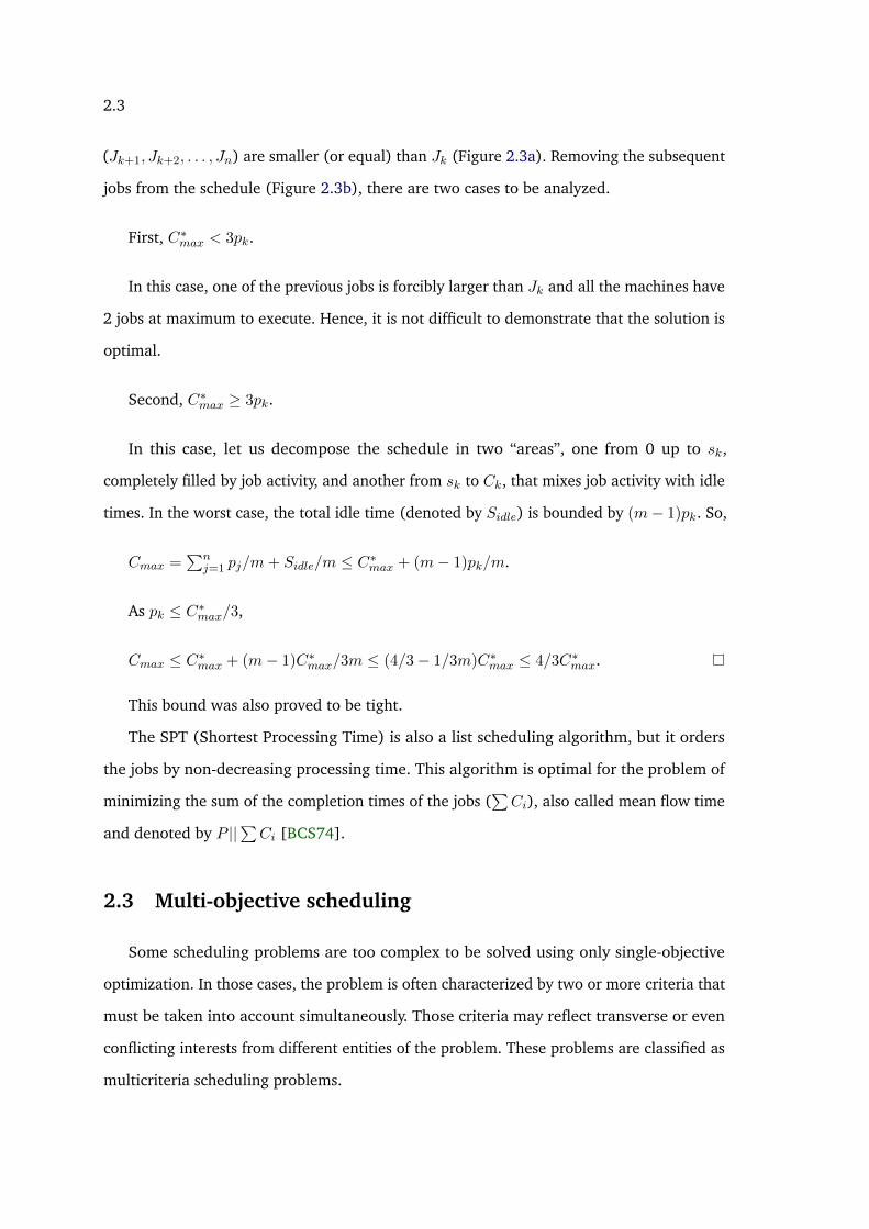
2.3

(Jk+1, Jk+2, . . . , Jn) are smaller (or equal) than Jk (Figure 2.3a). Removing the subsequent

jobs from the schedule (Figure 2.3b), there are two cases to be analyzed.

First, C∗max < 3pk.

In this case, one of the previous jobs is forcibly larger than Jk and all the machines have

2 jobs at maximum to execute. Hence, it is not difficult to demonstrate that the solution is

optimal.

Second, C∗max ≥ 3pk.

In this case, let us decompose the schedule in two “areas”, one from 0 up to sk,

completely filled by job activity, and another from sk to Ck, that mixes job activity with idle

times. In the worst case, the total idle time (denoted by Sidle) is bounded by (m− 1)pk. So,

Cmax =∑n

j=1 pj/m+ Sidle/m ≤ C∗max + (m− 1)pk/m.

As pk ≤ C∗max/3,

Cmax ≤ C∗max + (m− 1)C∗max/3m ≤ (4/3− 1/3m)C∗max ≤ 4/3C∗max.

This bound was also proved to be tight.

The SPT (Shortest Processing Time) is also a list scheduling algorithm, but it orders

the jobs by non-decreasing processing time. This algorithm is optimal for the problem of

minimizing the sum of the completion times of the jobs (∑Ci), also called mean flow time

and denoted by P ||∑Ci [BCS74].

2.3 Multi-objective scheduling

Some scheduling problems are too complex to be solved using only single-objective

optimization. In those cases, the problem is often characterized by two or more criteria that

must be taken into account simultaneously. Those criteria may reflect transverse or even

conflicting interests from different entities of the problem. These problems are classified as

multicriteria scheduling problems.

2.3

Let us assume, for example, that there are two criteria X1 and X2 to be minimized. If

X1 is considered to be more important than X2, a natural approach is, first, to find the

optimal value of X1, denoted by X∗1 , and then, in a second stage, optimize X2 subject to

the additional constraint that X1 ≤ (1 + η)X∗1 , where η as a given threshold (possibly 0).

This approach is called hierarchical (or lexicographic) optimization [Hoo05]. If both criteria

are considered equally relevant, then a different view of simultaneous minimization refers

to the concept of non-dominated – or Pareto optimal – solutions.

This concept was first used by Vilfredo Pareto, an Italian economist, in his studies of

economy efficiency and income distribution. This concept captures the trade-off between

two or more objectives to be optimized and can be used for comparing multi-objective solu-

tions. In this context, a solution A is better than a solution B if B is Pareto dominated by A.

Intuitively, a solution A is Pareto optimal if it is not possible to improve one of its objectives

without worsening the others. Next, we borrow the definition of Pareto dominance and

Pareto optimality from [Voo03] and [Hoo05], considering X = {X1, X2, . . . , Xk} as a set

of objectives to be minimized and a pair of schedule solutions S and S′.

Definition 2.1. A solution S Pareto dominates a solution S′ ⇔ ∀l ∈ {1, . . . , k}, Xl(S) ≤

Xl(S′)

and ∃l ∈ {1, . . . , k}|Xl(S) < Xl(S′)

Intuitively, this means that if S Pareto dominates S′ then values on S are equal or less

than S′ values, being that at least one of the inequalities is strict. Solutions that are not

Pareto dominated by any other solution is said to be Pareto optimal.

Definition 2.2. Schedule S is Pareto optimal or non-dominated if there is no feasible schedule

S′ 6= S such that S′ Pareto dominates S.

In multi-objective optimization problems, we are interested in finding solutions that are

not Pareto-dominated by any other solution. This set of non-dominated solutions is called

the Pareto set.

Figure 2.4 shows a visualization of a Pareto set for a multi-objective problem with two

objectives, X1 and X2. The points A, B, C, D, E and F are all possible solutions to the

2.3

A

BC

Z

N

D

E

F

X1

X2

Pareto set

Figure 2.4: Pareto set for the set of solutions X = {X1, X2}

problem. The point Z, called Zenith, represents the best possible solution to X1 and X2, if

they were considered individually, in a dedicated system. In contrast, the point N , called

Nadir, represents the worst possible solution for both objectives. In this figure, the Pareto

set is represented by the curved line. The points A, B, C, D are Pareto optimal, while

points E and F are Pareto dominated.

The main works related to this thesis address the problem of optimizing criteria from

many users simultaneously. This problem was first studied on a single processor with

two users by Agnetis et al. [AMPP04] and extended to multiple processors by Saule and

Trystram [ST09].

Agnetis et al. [AMPP04] analyzed several scenarios with two users varying the objective

function adopted by each one and the structure of the processing system. They were

interested in Constrained Optimization Problems where one objective is fixed as a constraint

while the second objective is optimized. Following the Graham classification scheme, this

problem is indicated as 1||fA : fB ≤ Q where fA and fB are the objective functions of

the users and Q is an integer. Formally, the problem is to find a schedule α∗ such that

fB(α∗) ≤ Q, and fA(α∗) is minimum. Given this, they provided a < 1, 1 >-approximation

polynomial algorithm for the problem of two users interested in minimizing their makespan

on a common processing resource. This notation means that for given w = (w1, w2)

thresholds for the values of the objective functions f (1), f (2), the algorithm delivers a

solution where f1 ≤ 1.w1 and f2 ≤ 1.w2.

2.3

The authors also show that when both users are interested in the sum of completion

times, the problem becomes also binary NP-hard and they provide a pseudo-polynomial

dynamic program to solve it. With mixed objectives, if one user is interested in the weighted

sum of completion times, the problem is binary NP-hard. Other cases are polynomial.

Saule and Trystram [ST09] analyzed the Multi-Users Scheduling Problem (MUSP),

namely, the problem of scheduling independent sequential jobs belonging to k different

users on m identical processors. In this problem, each user selects an objective function

among makespan and sum (weighted or not) of completion times. This is an offline problem

where all the jobs are known in advance and can be immediately executed. This problem

becomes strongly NP-hard as soon as one user aims at optimizing the makespan. For the

case where all users are interested in the makespan, denoted by MUSP (k : Cmax), the

authors showed that the problem can not be approximated with a vector ratio better than

(1, 2, . . . , k). This is a natural extension of the approximation ratios notation where the u-th

number of the vector corresponds to the approximation ratio on the u-th user objective.

The term “no vector-ratio better than (ρ1, ρ2, . . . , ρk)” stands for the component wise

relation, which means that the vector-ratio (ρ1, . . . , ρi−1, ρi − ε, ρi+1, . . . , ρk) is not feasible.

However, this formulation does not prevent a (ρ1, . . . , ρi− ε, . . . , ρj + ε, . . . , ρk) vector-ratio

from existing. For example, consider the vector-ratio H = (3, 3, 3, 3). If there is no vector-

ratio better than H, then the vector-ratio (3, 3, 2, 3) is not feasible while (4, 3, 2, 3) may be

feasible.

1

1

1

1

1

1

m

1

1

1

...

...

n

... ...

... 1

1

1

1

1

1

1

1

1

...

...

... ...

...

n

1

1

1

1

1

1

1

1

1

...

...

... ...

...

...

n

User k

User 1

User 2

User k

...

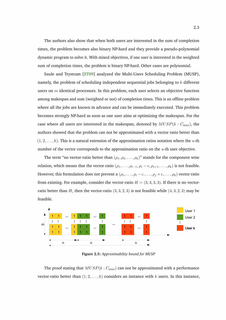
Figure 2.5: Approximability bound for MUSP

The proof stating that MUSP (k : Cmax) can not be approximated with a performance

vector-ratio better than (1, 2, . . . , k) considers an instance with k users. In this instance,

2.3

each user has m.n jobs, where m is the number of machines and n is any integer. All the

jobs have the same length p = 1 and the absolute best makespan that can be achieved

for each user is n, while in any efficient schedule one user will have a makespan of n,

another one will have a makespan of 2n, and so on until the last user with a makespan of

kn. Thus, it is impossible to obtain an algorithm that guarantees a vector-ratio better than

(1, 2, . . . , k). This can be easily visualized in Figure 2.5.

Note that in an efficient schedule, the set of jobs of one user is scheduled all at once, as

a single block. Each user block is followed by another user block, the resulting schedule

being all the users blocks, one after the other. If we take a job scheduled at time ti and

change its position with a job from another user scheduled at time tj > ti, we end up with

a schedule whose vector-ratio is worst than (1, 2, . . . , k) since two users will have tj as their

Cmax values. The resulted vector-ratio will be (1, 2, . . . , tj , tj , . . . , k), where the values are

in non-decreasing order. This is analogous for the case ti > tj .

Figure 2.6 illustrates the trade-offs between the objectives of two users. As a matter of

simplicity, only a single machine is used in this example. In this figure, user 1 (light gray)

owns two jobs of length 4, while user 2 (dark gray) has two jobs of lengths 3 and 7. All

the scheduling possibilities are presented as points on the graph, where C1max in the x-axis

and C2max in the y-axis represent the Cmax values of user 1 and user 2, respectively. Point Z

represents the Cmax lower bound of both users (zenith), while the upper bound (nadir) is

unlimited1. Points A and E are optimal in the sense that there is no better solution that

improves one objective without degrading another one. Points B and F are derived from A

by exploring different positions for the first job of user 2. But both solutions degrades the

Cmax of user 1 without improving the Cmax of user 2. The same applies for points C and D

relative to E. Thus, according to the concept of Pareto dominance, we say that B, C, D,

and F are Pareto-dominated solutions.

Based on these observations, Saule and Trystram [ST09] proposed an algorithm for

MUSP (k : Cmax) called MULTICMAX and proved that it is a (ρ, 2ρ, . . . , kρ)-approximation.

Each position of this vector ratio represents the performance ratio of one of the k users1Empty spaces between jobs can push both Cmax values to an unlimited extent.

2.3

3 74 4

8 18

10

18A

A

11

B

C

D

E

F

B,F14

C,D

EZ

A

C1

max

C2

max

Figure 2.6: Pareto optimality for MUSP (user 1 in light gray, user 2 in dark gray)

and ρ is the approximation ratio of an algorithm for the single-user case (Hochbaum and

Shmoys proposed a PTAS to this problem by using dual approximation [HS87]). They also

proposed an algorithm (called MULTISUM) for the case where all users are interested in

the sum of completion times and proved that it is a (k, . . . , k)-approximation.

The algorithm MULTICMAX works as follows: for each user u, it computes a schedule

Su with a ρ-approximation algorithm. Then, it sorts the users by non-decreasing values of

Cumax(Su), where Cumax(Su) denotes the Cmax value of schedule Su. Finally, it schedules the

jobs of user u according to Su between Σu′<uCu′

max(Su′) and Σu′≤uCu

′max(Su

′). Examining

again the example of Figure 2.6, the solution A would be the one generated by this

algorithm.

The theorem and the proof stating that MULTICMAX is a (ρ, 2ρ, . . . , kρ)-approximation

of MUSP (k : Cmax) can be seen in [ST09]. This theorem is valid for a given unknown

permutation of users as one user can not know in advance his/her rank in the algorithm.

The vector-ratios are computed relatively to an absolute best solution which is usually un-

feasible, but the authors emphasize that this is reasonable since it ensures the performance

degradation of each user.

Indeed, this algorithm generates a final schedule that might contains idle spaces. Those

may appear between two consecutive blocks of jobs from different users, allowing many

portions of the system to remain unusable. As an example, consider an instance with

2.4

two users, each of them with bm/2c jobs of length p and m > 1 (number of machines).

MULTICMAX generates a final schedule of length 2p using bm/2c machines, while the

optimal schedule is of length p, with each user occupying one half of the machines. But this

is a situation where the absolute best makespan for both users is feasible, which is not the

general case. So, still in this work, the authors presented a class of solutions where each

user submits a reasonable number of jobs that follows a linear function on the number of

machines. They showed that this class of solutions are MULTICMAX with ρ = 2 and that it

contains efficient schedules that are close to the Pareto set.

2.4 Fairness in scheduling

Fairness is an important issue while designing scheduling policies and it has gained

growing attention from computer scientists in the last decade [SKS04, SS05, RLAI04, VC05,

IPC+09, CM10, Pro13, KPS13]. However, it is still a fuzzy concept that has been handled

in many different ways, varying according to the target problems. It is said that resources

are fairly shared if they are equally available to the parties, or are available in proportion

to some criterion (e.g. money income, user hierarchy, etc.) [Dro09]. The definition of

available and equity, however, are subject to interpretation.

For example, if the resource is shared by three users, namely A, B and C, and they

are assigned shares x, y and z, then their jobs will receive fractions xx+y+z , y

x+y+z , zx+y+z ,

respectively. For a resource to be equally available, it can be determined that all the parties

have an equal share of the resource at any time moment. In this example, this would be

x = y = z = 1/3.

There are two classical approaches to share a resource in a system: space sharing and

time sharing. In space sharing, the resource is divided into subsets that are assigned to each

party. This can be more easily applied to divisible resources such as computer memory,

bandwidth and parallel systems. For indivisible resources like single processing units and

I/O devices, time sharing may be a more appropriate approach, since it gives time slices to

the parties in a round-robin fashion. During each time slice the resource is available to just

one user.

2.4

Figures 2.7 and 2.8 are examples of space-sharing and time-sharing schedules. In these

examples, a parallel machine with m processors is shared by 3 users identified by different

shades of gray and each user has the same share of the processors.

�

�

����

���

Figure 2.7: Space-sharing schedule example with 3 users

�

�

����

���

Figure 2.8: Time-sharing schedule example with 3 users

Users’ satisfaction or wishes (i.e. utilities), however, is a function of not only the assigned

resources, but also the needs. If the needs are unequal, even if the resources are allocated

according to the assigned shares, the resulting utilities will differ.

For instance, consider a system with m processors shared by two users u and v. User u

submits a sequential job of 10 hours of processing time while the user v submits m jobs of

one hour each. Assume the jobs are non-preemptive.

Using a time-sharing algorithm, one user will be executed after the other in their

respective time slices. In this case, the time slice must be equal or greater than 10 hours.

Otherwise, the job of u would never get executed. But even so, executing one user after

the other in distinct time slices will produce different utilities since one user needed a

processing time 10 times larger than the other and waiting 10 additional hours has different

impacts for each user.

2.4

In turn, using a space-sharing algorithm implies in giving to users u and v half of the

processors. However, it is clear that giving half of the processors to user u, that needed

only one processor, results in a different utility than giving the other half to the user v, that

needed all the resources to speed up the execution of his/her jobs.

Moreover, sharing of resources according to space-share policy may be Pareto-inefficient.

Consider another example with two users submitting m jobs of one hour each, with each

user being given half of the processors. In this case, both users will wait 2 hours. If instead

all the processors would be given to one user and then to the other, the completion time

of the first user would be improved, while the completion time of the second user would

remain the same.

This example is depicted in Figure 2.9 where C1max is the makespan of dark gray user

and C2max is the makespan of light gray user. The space-share solution represented by B is

Pareto dominated by the time-share solution represented by A.

�

�

��

���

��

���

�

�

�����

�

�����

��������

����������

�

��������������

�� �� � �

Figure 2.9: Examples of space-share and time-share schedules with 2 users and corresponding Paretosolutions

In fact, neither strict space-sharing nor strict time-sharing can solely produce reasonable

fair schedules in parallel systems. In this thesis it is shown how this can be achieved through

a combination of both strategies, embedded with a fair allocation policy. But first, it has to

be defined how fairness and utilities are formally measured.

Throughput-oriented users, for example, are interested in maximizing the job through-

put, i.e. number of jobs executed per time unit. So, maximize the minimum throughput is

2.4

the correct measure for having a greater number of satisfied users. In turn, response-time

oriented users – the type of interest in this work – are concerned about minimizing the job

response time (also called flow time), i.e. the time their jobs spent in the system. Likewise,

minimize the maximum flow-time (i.e. max-flow-time) seems to be the right measure.

However, flow time solely is not appropriate, because giving the same flow time for all jobs

results in worst performances for short jobs, compared to the ones obtained by long jobs.

So, in order to do a correct comparison, the job lengths must be taken into account. The

stretch metric is the one used to comply this.

The stretch is defined as the flow time normalized by the job’s processing time. More

formally, considering a job J, the stretch of J is:

J’s completion time - J’s submission timeJ’s processing time .

The stretch and flow metrics were first studied by Bender et al. [BCM98] for contin-

uous job streams. Stretch optimization was also studied for independent tasks without

preemption [BMR02], Bag-of-Tasks applications [LSV06, CM10], multiple parallel task

graphs [CDS10] and for sharing broadcast bandwidth between clients requests [WC01].

A job stretch measures how the performance of a job is degraded compared to a system

dedicated exclusively to this job. Thus, the stretch measures the relative responsiveness of

the system and quantifies the user expectation that the flow time should be proportional

to the imposed load. For example, it may be fine for a 2 hours job to be executed within 3

hours since its submission (resulting in a stretch of 1.5). However, for a 30 minutes job this

delay may be unacceptable (it would result in a stretch of 6).

As an analogy with the concept of distributive justice presented in the introduction, two

jobs J1 and J2 are equally treated if they have the same stretch. That is:

J1’s completion time - J1’s submission timeJ1’s processing time =

J2’s completion time - J2’s submission timeJ2’s processing time .

The completion time is the job “reward”, that is, what is obtained from the scheduler.

In this case, the lower, the better. The submission time represents the job “cost” in terms of

scheduling effort: the sooner a job was submitted, less effort is needed from the scheduler

to deliver the expected “reward”. Finally, the processing time is the job “investment” in

2.4

an inversely proportional relation: short processing times represents more investments to

achieve better rewards than long processing times.

In this thesis, the stretch metric is adapted to the notion of job campaigns. This is

detailed in Chapter 3.

In order to optimize stretch, it is worth to analyze some strategies. Unfortunately,

common approaches such as First-Come-First-Served (FCFS) and classical list scheduling

strategies are not well-adapted. FCFS is maybe the simplest and still more largely used

scheduling algorithm. It executes jobs according to a FIFO order (First In, First Out), that

is, in the order that they arrive in the system. Other well known scheduling policies as

LPT [Gra69] (Longest Processing Time first), SPT [BCS74] (Shortest Processing Time first)

and their derivatives focus on job lengths to achieve single objective optimization such as

overall makespan or throughput. The execution priority is given individually to the jobs

according to their lengths. In LPT, longer jobs have bigger priorities while in SPT, shorter

jobs are prioritized.

� � �

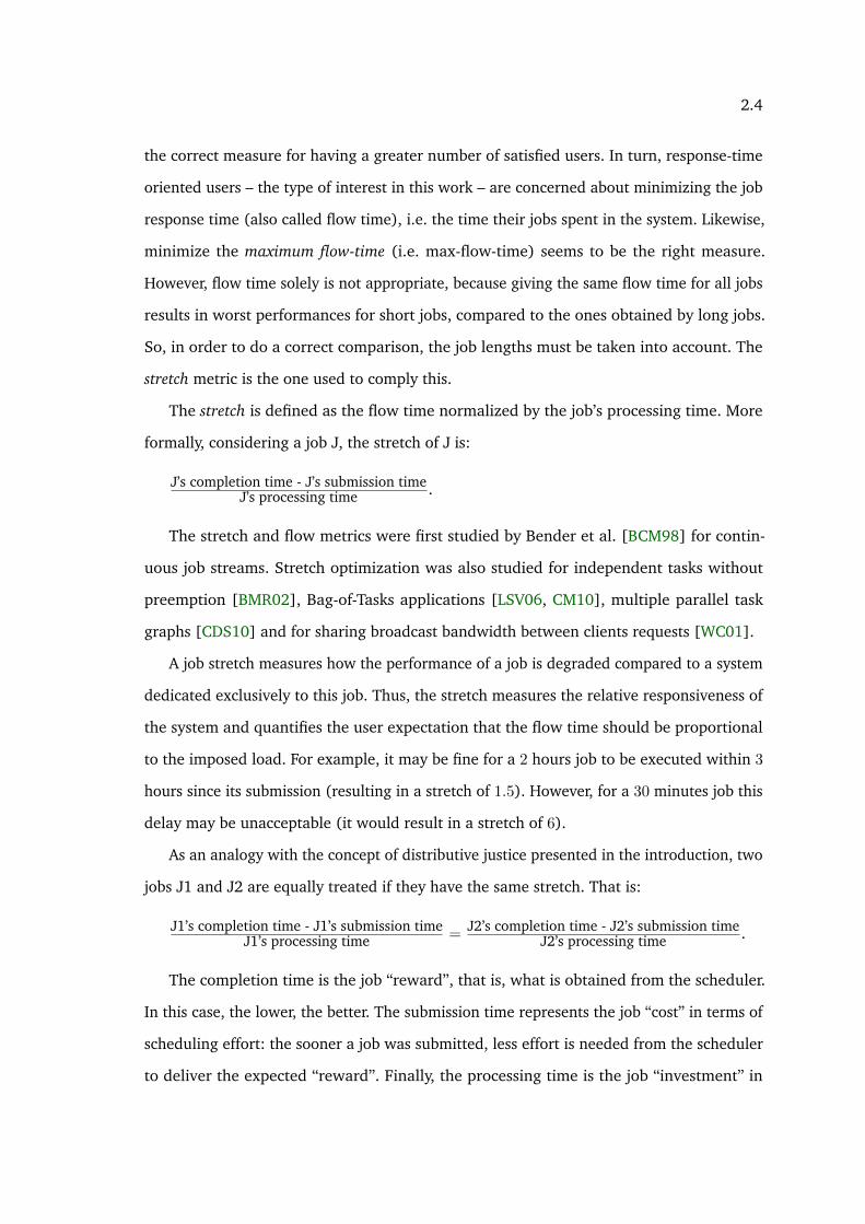
Figure 2.10: FCFS worst-case ratio with 2 users

Figures 2.10, 2.11 and 2.12 illustrate examples of schedules constructed by FCFS, LPT,

and SPT algorithms. In these figures, two users, identified by two shades of gray, submit

their parallel jobs of length 1 and p on a single machine. All the jobs are ready to execute

from the beginning of the schedule. It is well-known that these policies do not embrace user

related information such as user identity and submission frequency. Hence, they do not

grasp the sense of justice in a multi-user environment. But, even if they did, these policies

could bring very bad stretch experiences to users.

FCFS, for instance, can be unfair to users who always submit small jobs. One can easily

realize that a small job can wait an arbitrarily long time to start since the system is fully

occupied with the execution of jobs submitted earlier by another users. Assuming, for

2.4

example, that both users start submitting jobs at time 0 and that each job of a user is

submitted as soon as the previous finishes, one user can be systematically delayed by the

other. This is depicted in Figure 2.10 where the resulting stretch for the dark gray user is

far from the optimum by a factor of 2p.

� � �

���

Figure 2.11: LPT starvation with 2 users

� �� �

���

�� � �

Figure 2.12: SPT starvation with 2 users

In turn, policies whose ordering is based on job length like SPT and LPT are subject

to job starvation if applied without a dynamic priority mechanism. These are the cases

depicted in figures 2.11 and 2.12. In both figures, new arriving jobs from the light gray

user can indefinitely delay jobs from the dark gray user. In those cases, the resulting stretch

for the dark gray user can be arbitrarily far from the optimum.

When it comes to policies and mechanisms implemented on actual systems like

PBS [Hen95], OAR [CDCG+05] and Slurm [YJG03], most of them supports multilevel

queue scheduling and backfilling. Multilevel queue scheduling is a powerful mechanism on

which jobs are organized into different queues according to some classification criterion.

Each queue is given a distinct priority and the jobs are FIFO ordered and executed. It is

often used to separate different types of jobs (e.g. batch, interactive, etc.) or to reflect

the user hierarchy of the system (e.g. administrator jobs could be placed on a different

queue than user jobs). So, regarding fairness between users, priority queues are as fair as

hierarchical systems can be, if used solely.

Backfilling can be used to fill the idle gaps between jobs and increase system utilization.

2.4

It consists in searching for idle spaces backwards in the schedule in which upcoming jobs

can be placed. This can be done in a more or less aggressive way regarding the delay of

previously scheduled jobs. This technique does not deliver individual guarantees to users

regarding performance neither equitable treatment [SKSS02], however, it is a powerful

mechanism that, in practice, offers significant scheduler performance improvement.

In [RLAI04] and [SKS04], several metrics are proposed for expressing the degree of

unfairness in various systems. Both works evaluate the unfairness of algorithms such as

FCFS, backfilling and processor sharing, but fairness is associated with the jobs and their

service requirements. Thus, the concept of fairness is always taken from a job point-of-view

as “fairness between jobs” instead of “fairness between users” as it is supported in this

thesis.

In the real world, fair-share derived mechanisms are implemented by some parallel

system schedulers. Some examples are the Hadoop Fair Scheduler [Zah], the fair-share

policy of Maui Scheduler [JSC01] and the Fair-share Factor of Slurm Multifactor Priority

Plugin [YJG03, Geo10].

In Hadoop, fairness is obtained by space-sharing. It divides the resources among distinct

pools, each one belonging to a user. Figure 2.13 depicts a space-share schedule with the 6

resources being equally divided among 3 pools. At the beginning, M1, M2, and M3 belong

to the pool of dark gray user, while M4, M5, and M6 belong to the pool of medium gray

user. At time t = 2 the light gray user joins the system. Now, M1 and M2 form the dark gray

pool, M3 and M4 form the light gray pool, and M5 and M6 form the medium gray pool. The

pools are also changed in t = 8 and t = 12 as users leave the system. In Hadoop, weights

can be applied to the pools, giving more or less priority to them, but in this example all

pools have the same weight.

Observe that, using space sharing, the stretch experienced for each user is linearly

proportional to the number of users. All the user workloads are equally stretched and, thus,

the schedule is fair.

However, this solution has some drawbacks. First, the jobs are assumed to be malleable.

But when scheduling rigid or moldable jobs, the final schedule would be hardly seamless

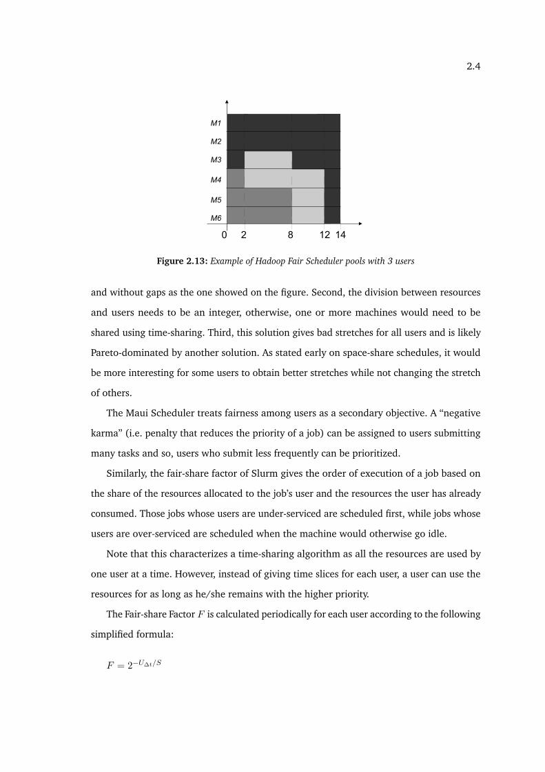
2.4

��

��

��

��

��

��

�� �����

Figure 2.13: Example of Hadoop Fair Scheduler pools with 3 users

and without gaps as the one showed on the figure. Second, the division between resources

and users needs to be an integer, otherwise, one or more machines would need to be

shared using time-sharing. Third, this solution gives bad stretches for all users and is likely

Pareto-dominated by another solution. As stated early on space-share schedules, it would

be more interesting for some users to obtain better stretches while not changing the stretch

of others.

The Maui Scheduler treats fairness among users as a secondary objective. A “negative

karma” (i.e. penalty that reduces the priority of a job) can be assigned to users submitting

many tasks and so, users who submit less frequently can be prioritized.

Similarly, the fair-share factor of Slurm gives the order of execution of a job based on

the share of the resources allocated to the job’s user and the resources the user has already

consumed. Those jobs whose users are under-serviced are scheduled first, while jobs whose

users are over-serviced are scheduled when the machine would otherwise go idle.

Note that this characterizes a time-sharing algorithm as all the resources are used by

one user at a time. However, instead of giving time slices for each user, a user can use the

resources for as long as he/she remains with the higher priority.

The Fair-share Factor F is calculated periodically for each user according to the following

simplified formula:

F = 2−U∆t/S

2.4

where S is the normalized share and U∆t is the normalized usage factoring in half-life

decay.

In a system with k users and no user hierarchy, the normalized share S = 1/k and the

normalized usage is calculated as:

U∆t = Uuser(∆t)/Utotal(∆t)

where Uuser(∆t) is how much time the jobs of the user consumed from the processors over

a fixed time period ∆t and Utotal(∆t) is the total consumption from all the jobs over that

same time period.

So, the factor F is a value between zero and one, where one represents the highest

priority and zero the lowest. A factor of 0.5 indicates that the user has used exactly the

portion of the machine that was allocated to him/her, above 0.5 it indicates that the user

has consumed less than the allocated share, and below 0.5 it indicates that the user has

consumed more than the allocated share. The user factors are recalculated periodically

according to a predefined time interval ∆t and the user with the highest factor value has

the highest priority.

��

��

��

��

��

��

�� ��� � � �� ��

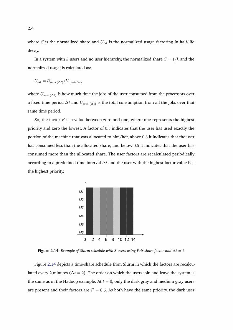
Figure 2.14: Example of Slurm schedule with 3 users using Fair-share factor and ∆t = 2

Figure 2.14 depicts a time-share schedule from Slurm in which the factors are recalcu-

lated every 2 minutes (∆t = 2). The order on which the users join and leave the system is

the same as in the Hadoop example. At t = 0, only the dark gray and medium gray users

are present and their factors are F = 0.5. As both have the same priority, the dark user

2.4

is randomly chosen and until t = 2 only dark gray jobs are executed. At t = 2 the factors

are recalculated. Also, the light gray user joins the system. Now, the dark gray user has

F = 0.125 while the other users have F = 1. As light and medium gray users have the

same priority, the light gray user is randomly chosen and until t = 4 only light gray jobs are

executed. This process is repeated at every time interval until all jobs get executed. Note

that from t = 10 there is only dark gray jobs to be executed and so there is only dark gray

jobs until the end.

This solution has some advantages over the Hadoop Fair Scheduler. First, each user

gets all the resources, so the problem of dividing the resources evenly between users is no

longer present. Second, it is more responsive: the stretches for each user workload were

equal or better than the ones in the space-share schedule of Hadoop.

However, this solution has also some drawbacks. Similar to Hadoop, the final schedule

would be hardly seamless and without gaps when scheduling rigid or moldable jobs. Further,

users get bad factors for using the resources even when there is no other user present on

the system. Ideally, no user should be punished for making use of resources that would be

idle otherwise [Dro09].

Chapter 3

The Campaign Scheduling Problem

Computing infrastructures for parallel processing are generally multi-user, requiring

that users, alone or grouped in projects, share the same environment to perform theirs jobs.

In HPC clusters, for example, several processors are grouped to empower the execution

of CPU intensive applications from diverse research fields as particle physics, weather

prediction, seismic data processing, and bio-informatics.

The management of processors is commonly done by a Resource Management System

(RMS) whose main part is the job scheduler. Typically, jobs are submitted in batch and

placed on one or several queue(s) before being executed.

In a typical shared parallel system, each user performs many submissions over time

driven by scientific questions related to the project he/she belongs to. Some users may

perform many submissions with few jobs in a short period of time, while others may

perform few submissions with many long jobs in a very sparse way. In short, daily scien-

tific activities such as exploratory analysis, simulations, fine-tuning, system prototyping,

algorithm comparison, and benchmarks are commonly performed several times interleaved

by idle time periods during which the users may analyze previous results or prepare their

next submissions. This user activities towards a common goal can be seen as a many-step

interactive workflow where each step is called a “campaign”.

In this thesis, we fit this notion of campaign in what we called the campaign model.

31

3.2

3.1 The campaign model

A campaign is composed of jobs and the job scheduler is responsible for organize the

campaigns, ordering their execution according to a specific policy. As soon the execution of

a campaign is finished the campaign owner is able to submit his/her next campaign. It is

clear that, from the user point of view, the sooner his/her jobs are executed, the better. So,

the objective of each user is to minimize the time each campaign spent in the system. It

starts with the submission and it ends when all the jobs are executed. Namely, this is the

campaign’s flow time.

To give an example, Figure 3.1 illustrates a campaign submission from a user in a system

with 4 machines (named M1, M2, M3 and M4). The medium gray rectangles represent jobs

from the user while the light gray rectangles represent jobs from other users. Note that, at

the time of the submission, all the machines are occupied so the campaign does not start to

be executed immediately.

������

��

��

�

������

��������

Figure 3.1: Campaign submission and execution on a 4 processor system

3.2 Related models

In this section, we present some examples of real application models and systems, and

how they are related to campaign scheduling.

3.2

3.2.1 Bag-of-Tasks

Bag-of-Tasks (BoT) is an application model composed of tasks to be executed inde-

pendently from each other. The tasks can be executed in any order and there is almost

no communication between them. There are only two points of communication: at the

beginning, for passing the initial parameters for each task, and in the end, for transmitting

the results.

The parallelization of these applications is so trivial that they are also known as

embarrassingly parallel applications. Some examples of areas that can make use of the

BoT model are data mining, Monte Carlo simulations, distributed rendering, and particle

physics. This model is often used in parallel system with communication constraints and

desktop based platforms like BOINC [And04].

3.2.2 Parameter sweep applications.

Another common example is found in parameter sweep applications. These applications

scan a wide range of possible parameter values and iteratively "zooms" into promising areas.

The computation is performed in stages: (i) testing multiple values of parameters; (ii)

choosing the most promising area and generating parameter values for the next iteration.

Stages are repeated until the quality of the obtained solution does not improve significantly

in subsequent iterations.

The summary step is easy to compute. It is performed either off-cluster, or in a central-

ized node. The most computationally-expensive step is the testing step. The application

can be modeled as a set of independent jobs {Ti}i=1,...,n. Each job is a set of files and a file

might be the input to one or more jobs. Each job tests a certain combination of parameters.

Jobs are moldable; they scale almost linearly up to a certain number of processors. The

runtime of jobs can be estimated.

3.2.3 BSP model.

The BSP is a programming model introduced by Leslie Valiant that combines soft-

ware and architecture [Val90]. Processing applications written using the BSP paradigm

3.2

is a twofold procedure: the program is a sequence of super-steps and each super-step

comprises three phases, namely computation, communication and global synchronization.

In the computation phase, each machine executes one sequential job. The computations

are independent in the sense that they execute asynchronously from all others. In the

communication phase, the jobs communicate between themselves to exchange data. When

a job has no more data to exchange, it enters in the synchronization phase where it waits

until all the jobs finish their communications.

One of the advantages of this model is its simplified interface, which facilitates the

implementation of BSP libraries and parallel applications based on the BSP model. Another

advantage is the performance predictability that can be analyzed assuming that one time

unit in one processor can perform one operation in a data available in its local memory.

But this model has also some disadvantages, as the need of periodic synchronizations

among the processes. This become very costly as the cluster becomes larger. Also, depending

of how frequent these synchronizations happen, the performance can be compromised.

3.2.4 Similarities and applicability

The examples presented on the previous sections share some characteristics with the

campaign model. In all of them each user shares the resources with others and performs

many submissions that composes the user workload. Terminologies like batch, stage, phase,

and step are interchangeable as they share the same concept of campaigns. Another point

in common is that applications fitting these models are more likely to be response-time

based than throughput based. When a campaign is submitted, users want to gather the

partial results as quickly as possible in order to prepare the subsequent campaign. But,

despite these similarities, there are some particular differences regarding mainly the job

model, the time interval between campaigns, and the level of clairvoyance.

These models, for example, do not specify job preemptiveness. This is defined by

the model implementation on a particular system. Most BOINC projects, for instance,

implement the bag-of-task model using preemptive jobs. This means that the scheduler can

interrupt jobs of one user without loss of computation. Campaigns from two or more users

3.3

can even be split in several parts and interleaved, without idle spaces between them.

For the BSP, there is one straightforward approach to map this model into campaign

scheduling: each superstep can be seen as a single campaign. The length of each phase

is particular to each job and it depends on the machine that was allocated to it. But the

synchronization is a barrier that symbolizes the end of a campaign. As no campaign can

start before the end of the previous one, no superstep can start until the previous superstep

has ended. Two or more BSP applications competing for the same set of resources can be

expressed as a multi-user campaign scheduling problem. It is up to the scheduler to decide

the most honest way of sharing the resources among the applications.

Despite of the fork-join shape of these examples, the campaign model described in this

thesis can be applied to many situations since it models an execution pattern: submissions

of independent jobs from many users over time. Gathering partial results and elaborating

the next input can automatically be executed by one of the tasks like is done in BSP. In this

case, all the tasks are processed without idle times between campaigns. However, this is

not the general case.

In summary, human intervention between campaigns may take place or not. It depends

on the type of application and/or interaction with the system. In some cases, the user can

choose when the next submission will be released and, therefore, the time interval between

the campaigns can be arbitrary.

3.3 Definitions and notation

The model consists of k users (indexed by u) sharing the resources on a parallel

platform composed ofm identical processors managed by a centralized scheduler. Figure 3.2

illustrates some of the used notation.

A user workload is composed of successive campaigns where each campaign (indexed

by i) is submitted at a time denoted by tui and is composed of a set of independent and

non-preemptive jobs.

A campaign is defined as the set Jui containing the jobs released by a user u in one

submission; nui denotes the number of jobs of a campaign and nu the total number of jobs

3.3

���������������� ����������������

����

����������������

����������������

�������������

��

��

�

��

�

���

��

�

��

�

�

��

��

�

��

�

���

��

�

��

�

��

�

��

�

�

Figure 3.2: Campaign Scheduling with 2 users (user 1 in light gray, user 2 in dark gray)

released in all the campaigns of user u. The jobs inside a campaign are indexed by j, so Jui,j

denotes job j from campaign Jui .

The job’s length is denoted by pui,j and the job’s size is denoted by qui,j . So, the total

workload within campaign i is: W ui =

∑j p

ui,j .q

ui,j . But, when size is not mentioned, jobs

should be considered sequential. In these cases, W ui =

∑j p

ui,j . This is assumed in most of

this thesis, with the exception of Chapter 6.

A job, once started, cannot be interrupted nor preempted. The job start time is denoted

by sui,j and its completion time is denoted by Cui,j .

The start time of a campaign i of user u is denoted by sui . It is defined as the time the

first job starts, so sui � minjsui,j . The campaign’s completion time Cu

i is the completion time

of the last job to finish its execution: Cui � maxjCu

i,j .

The campaign’s flow time, denoted as ∆ui , is equal to the amount of time the jobs of a

campaign stay in the system: ∆ui � Cu

i − tui .

The campaign’s stretch is denoted by Dui and is defined as a natural generalization

of a job’s stretch. Formally, the stretch of job i, Dui,j , is equal to the relative degradation

of its flow time, Dui,j = (Cu

i,j − tui,j)/pui,j , where pui,j is the job length (and, thus, the job’s

3.3

Table 3.1: Notation summary

k number of usersu user indexi campaign indextui submission time of campaign i of user unui number of jobs of campaign i of user uJui,j job J of campaign i of user usui,j start time of job Jui,jCui,j completion time of job Jui,jpui,j length (processing time) of job Jui,jqui,j size of job Jui,jCui completion time of a campaign i of user uttui think time between the submission of campaign i and the end of campaign i− 1 of user u4ui flow time of campaign i of user u

Dui stretch of campaign i of user u

optimum flow time) [BCM98]. Determining a single campaign’s optimum flow time means

solving the general scheduling problem, which is NP-hard. Thus, instead, we use a lower

bound on campaign’s flow time defined by lui = max(W ui /m, p

umax), where pumax = maxj p

ui,j .

Consequently, the campaign’s stretch is defined as Dui = ∆u

i /lui .

User u cannot submit her/his next campaign i + 1 until her/his previous campaign

i completes, thus tui+1 ≥ Cui . The time between the completion of campaign i and the

submission of the next one (i+ 1), called the think time, is denoted as ttui+1 = tui+1 − Cui .

The notation is summarized in Table 3.1.

From an individual point of view, each user u wants to minimize the sum of campaigns’

lengths Σ∆ui = Σi(C

ui − tui ). This objective is justified by the interactive behavior of users

when submitting tasks on a cluster: each user is interested in quickly obtaining the results

of individual batches of jobs rather then the job throughput in a time frame.

Using a natural extension of the classical three-field notation α|β|γ introduced by

Graham, Lawler, Lenstra and Rinnooy Kan [GLLK79], the resulting problem can be denoted

by P |camp|∑

∆u.

However, from the perspective of collective justice, the objective (of the system sched-

uler) is to minimize the per-user and per-campaign stretch Dui . We consider stretch as it

weights the responsiveness of the system by the assigned load; it is natural to expect that

small workloads will be computed faster than larger ones. We consider the stretch on a

3.4

per-user and per-campaign basis, as this results in fairness of the system towards individual

users. Moreover, optimizing the stretch of each campaign (rather than the overall stretch)

guarantees that not only the final result, but also partial ones, are timely computed. In this

case, the resulting problem can be denoted by P |camp|max{Dui }.

The problem of minimizing per-user and per-campaign stretch Dui is NP-hard. Even

when restricted to a single user (k = 1) and to a single campaign, it is equivalent to

the classical problem of minimization of the makespan on identical parallel processors

(P ||Cmax) [ST09, PRT12].

In the offline version of the problem, all the campaigns are known in advance (the

number and the lengths of the jobs) and each campaign can be submitted immediately after

the completion time of the previous one. In the online problem, each campaign (including

its submission time) is unknown until it is submitted. From this point, the length and

duration of each job is available.

The offline model may seem with no applicability at first, since to predict the number of

campaigns and their respective job lengths is unrealistic. But this model is well-suited for

some types of applications, like clairvoyant fork-join applications. In this type of application,

each set of fork-type tasks can be mapped onto campaigns and each join task represents

a single-job campaign. Furthermore, the offline set can always be used as a reference to

analyze the competitiveness of online algorithms1.

In this thesis, both models are analyzed and solutions are given to them.

3.4 Offline scheduling of single user’s campaigns

In this section, we analyze an offline version of the multi-campaign problem restricted

to a single user. This problem constitutes an absolute lower bound for the multi-user case,

since no objective value can be lower for a user than the one achieved when she/he is alone

in the system. We denote this problem by P |camp|∑

∆ (i.e. without the superscribed u).

We show below that the problem is NP-hard. Then, we show that the optimal makespan1Competitive analysis is a method for analyzing online algorithms. In this method, the performance of an

online algorithm is compared to the performance of an optimal offline algorithm in which all the future jobsubmissions are known in advance.

3.4

of P |camp|∑

∆ with σ campaigns is at most σ times longer than the optimal makespan of

an instance with the same jobs, but no campaigns (i.e. the same as P ||Cmax in which all

the jobs are ready to execute from the beginning of the schedule). Finally, we show that a

ρ-approximation algorithm for P ||Cmax is also a ρ-approximation for P |camp|∑

∆.

Proposition 3.1. P |camp|∑

∆ is NP-hard. The boundary problem is P2|camp|Cmax. The

processing times are arbitrary.

Proof. (straightforward) The proof is by reduction from the two-processor scheduling

problem P2||Cmax. An instance of P2||Cmax can be converted to an instance of P2|camp|C

by placing all the jobs in the same campaign (Jj → J1,j).

For the subsequent analysis of this section, we use the concept of campaign-compact

schedule, which is defined as follows:

Definition 3.1. A campaign-compact schedule ςcc (also called a non-delay schedule) is a

schedule in which jobs from a subsequent campaign start immediately after the completion of

the previous campaign, i.e., ∀i ∈ {1, . . . , σ − 1}∃j : s(i+1),j = Ci.

In an offline model, it is enough to consider only campaign-compact schedules be-

cause, for a single user, the class of campaign-compact schedules represent all “reasonable”

schedules.

A schedule that is not campaign-compact can be transformed to a campaign-compact

schedule by shifting the campaign submission times to coincide with the completion of

their previous ones. This transformation reduces completion times of some jobs and the

length of the whole schedule. Thus, the optimal schedule is also campaign-compact. In the

remainder of this section, a schedule is always considered to be campaign-compact.

The following lemma binds the completion time Ci of a campaign with the durations of

the previous campaigns; moreover, it shows that Cσ =∑

∆.

Lemma 3.1. In a schedule, the completion time of the i-th campaign Ci is equal to the sum of

durations of the previous campaigns and the current campaign: ∀iCi =

i∑i′=1

∆i′

3.4

Proof. Follows directly from the definition of ∆i and the Definition 3.1.

The notion of a campaign restricts the set of feasible schedules; thus the optimal

schedule for the campaign problem P |camp|∑

∆ might be longer than the optimal schedule

for a similar instance with all the jobs in a single campaign.

Proposition 3.2. An optimal schedule for an instance of the problem P |camp|∑

∆ with σ

campaigns is at most σ times longer than the optimal schedule for an instance of P ||Cmax

with the same jobs, that is: C∗σ ≤ σC∗max, where C∗σ denotes the optimal completion time of

the σ-th campaign and C∗max denotes the optimal Cmax for P ||Cmax. This bound is tight.

Proof. First, from Lemma 3.1, C∗σ =∑σ

i=1 ∆∗i , where ∆∗i is the duration of the i-th campaign

in the optimal schedule. Second, given that each campaign is a subset of jobs, ∆∗i ≤ C∗max.

Thus,∑σ

i=1 ∆∗i ≤ σC∗max.

For the tightness of the bound, consider an instance with m jobs of unitary length

(remember thatm is the number of processors). An optimal schedule with a single campaign

schedules all the jobs in parallel, with the completion time of Cmax = 1. If all the jobs belong

to different campaigns (σ = n), they must be executed sequentially, thus∑σ

i=1 ∆∗i = σ.

Consequently, spreading the jobs in multiple campaigns “costs” the system at most σ

(the total number of campaigns).

Another interesting question is what is the impact of using a ρ-approximation algorithm

to schedule the jobs inside a campaign. The following result states that any ρ-approximation

algorithm for the standard job scheduling problem can be used to obtain a ρ-approximation

for the campaign problem.

Proposition 3.3. Any scheduling algorithm A that is a ρ-approximation for P ||Cmax is also

a ρ-approximation for P |camp|∑

∆. The algorithm for P |camp|∑

∆ (denoted by A-camp)

creates a schedule by, first, performing σ executions of A, that is, executing A separately for

each campaign; then shifting the schedule of the i-th campaign by Ci−1.

Proof. From Lemma 3.1, Cσ =∑

i ∆i. As the algorithm used to schedule each campaign is

a ρ-approximation, ∆i ≤ ρ∆∗i . Thus, Cσ ≤ ρ∑

i ∆∗i , and as C∗σ =∑

i ∆∗i , Cσ ≤ ρC∗σ.

3.5

In summary, the barrier between subsequent campaigns affects the system by increasing

the makespan at most σ times. Yet, the resulting Campaign Scheduling problem can

use the same algorithm as the similar standard scheduling problem to obtain the same

approximation ratio.

3.5 Offline scheduling with multiple users

In this section, we study the offline version of the Campaign Scheduling problem with

multiple users, denoted by P |camp|∑

∆u. In this scenario, the campaigns are clairvoyant

(i.e. all the jobs from all the campaigns are known in advance) and each user submits

all the campaigns at once to be scheduled in sequence. Even with this restriction, this

problem is NP-hard as the boundary problem with one user (P |camp|∑

∆) is NP-hard (see

Section 3.4).

First, it is shown that this problem cannot obtain a better approximation vector-ratio

than (1, 2, . . . , k)2. Then, we apply a multi-campaign version of the MULTICMAX algorithm

to obtain a (ρ, 2ρ, . . . , kρ)-approximation solution. Finally, we reason about the tradeoff

between fairness and performance on this solution and why it is not sufficiently fair.

Proposition 3.4. P |camp|∑

∆u can not be approximated with a performance vector-ratio

better than (1, 2, . . . , k).

Proof. Let us consider the following instance. All campaigns of all k users have m jobs of

unitary length, where m is the number of machines. All users have the same number n of

campaigns. Obviously, for each user independently, the best∑

i ∆ui achievable is equal to

n. But, in any efficient schedule, one user will have∑

i ∆ui equal to n, another one will

have∑

i ∆ui of 2n and so on. Thus, it is impossible to guarantee a vector-ratio better than

(1, 2, . . . , k).

Remark that any permutation of this vector-ratio can be obtained (as explained in

Section 2.3). But this vector-ratio is not accomplished by all schedules. Consider for example

a schedule that interleaves campaigns of users similarly to the round-robin scheduling.2The meaning of term “no vector-ratio better than..” is recalled from Section 2.3

3.5

Each ∆ui will be of length 1. So, in this schedule, one user will have

∑∆ui = kn, another

one will have kn− 1, and so on until kn− k. Clearly, the corresponding vector-ratio will be

worse than (1, 2, . . . , k).

Based on this observation, we propose the MULTICAMP algorithm. This is an algorithm

for the offline problem inspired on the MULTICMAX algorithm [ST09] as it schedules users’

campaigns in blocks.

First, for each campaign i of each user u, the algorithm computes a schedule ςui . Usually,

ςui will be distant from the optimal by a factor. We denote this approximation factor as ρ.

Then, for each user, the algorithm puts all its campaigns’ schedules side by side to form a

single block, i.e. a campaign-compact schedule ςu (see Definition 3.1). The length of this

schedule ςu is∑

i ∆ui . Next, the users are sorted by non-decreasing values of

∑i ∆u

i . Finally,

the algorithm places the block ςu of user u between∑

u′<u

∑i ∆

(u′)i and

∑u′≤u

∑i ∆

(u′)i .

Proposition 3.5. MULTICAMP is a (ρ, 2ρ, . . . , kρ)-approximation algorithm of P |camp|∑

∆u.

Proof. First, we have to verify the validity of the final schedule. In fact, the campaign’s

blocks are scheduled in disjoint intervals of length∑

i ∆ui (ςu) according to ςu. Second, we

verify that the final schedule has a performance vector-ratio of (ρ, 2ρ, . . . , kρ). The users

are ordered by increasing values of∑

i ∆ui (Sui ) and each block is scheduled in sequence

according to this order. Thus,∑

i ∆ui ≤ u

∑∆ui (Sui ). Moreover, ςui was generated by a

ρ-approximation algorithm. Thus,∑

i ∆ui ≤ u

∑ρ∆u∗

i = uρ∑

∆u∗i .

Usually, a performance vector-ratio depending on k, a parameter of an instance, is not

considered as an efficient solution. However, the optimal value of each particular objective

function is obtained by scheduling the jobs of the user as if she/he was the only user on the

system. The performance vector-ratio represents the distance between the schedule given

by our algorithm and these absolutely optimal solutions for every user (the zenith point).

In the general case, the zenith solution is not feasible.

In MULTICAMP, although the response time of an entire block of campaigns of a user

(i.e. the total user workload) is bounded, individual campaigns are arbitrarily delayed. User

u may be disappointed that he/she has to wait u − 1 workloads to be processed before

3.6

his/her own workload starts to be executed. It should be more fair to the users if everybody

was equally affected or proportionally affected according to their own workload lengths.

In Section 2.3 we saw that, considering just one campaign (as in the MUSP problem),

is not a good idea to interleave jobs as it leads to inefficient, Pareto dominated solutions.

However, Pareto efficient solutions inherit an imbalance between users with respect to the

response time, given that campaigns are ordered according to their lengths. With multiple

campaigns, we can reduce this imbalance by giving higher priority in the next scheduling

decisions for the users that were “unhappy” in the previous ones. We tackle this problem in

the next section.

3.6 Online scheduling with multiple users

The offline solution is not suitable for the online version of the problem because

campaigns are unknown until they are submitted. The scheduler has no knowledge about

the user’s will to submit more campaigns than the ones that were already submitted, so it

is impossible to sort and prioritize users according to the total workload lengths.

An online algorithm should consider both user fairness and performance. As we do not

know the lengths of the workloads in advance, both criteria should be respected at any

time.

In this section, we first discuss how the stretch metric must be taken into account in

order to provide a fair mechanism in an online fashion. Then we analyze the performance

of the FCFS algorithm as it is the most used and well known online algorithm. We show

that FCFS is not suitable for fair scheduling in the way we defined since it can produce an

arbitrary large stretch for campaigns.

This section also serves as a preamble of the next chapter where more sophisticated

online solutions are proposed.

3.6.1 Measuring fairness by max-stretch

A scheduling algorithm is unfair if it gives preference to the applications which use

resources in a certain way, like preferring short running applications over long running

3.6

ones [SS05]. In this sense, FCFS can be considered fair if “equity” between applications is

the only think that is at stake since it treats all the applications in the same way, considering

only the arrival time to order their executions.

Nevertheless, FCFS may lead to long wait times and does not take into account that

different applications may belong to different users. In practice, some users may be inad-

vertently preferred. Yet, an algorithm considered “fair” for some context (and for some

definition of “fairness”) may not hold its properties in other contexts.

As each user is interested in the sum of campaigns’ response times, we tackle the

problem of fairness by measuring the campaign stretch. Recall that, for campaigns, the

stretch of a campaign is defined as the time the campaign stays in the system normalized

by the campaign’s lower bound on the processing time.

To guarantee fairness between users it is necessary to choose an aggregation function.

Three of them are normally considered, corresponding to the standard norms L∞, L1, L2:

minimizing maximum of stretches, sum of stretches, and product of stretches. From Sec-

tion 2.3, recall that improving the objective of a user in a Pareto-optimal solution implies

worsening the objective of other users. So, we consider that a Pareto optimal solution that

gives the same stretch for all the campaigns is more fair than a Pareto optimal solution that

gives different stretch values, even if the second produces a lower stretch sum.

According to this, a fair scheduling algorithm should strive to minimize the max-stretch

because this has the side effect of producing close stretch values for all users. Thus,

minimizing the max-stretch (maxuDu) is the natural choice.

3.6.2 FCFS in multi-user systems

FCFS is one of the most commonly used policies in job scheduling and this can be

justified not only by its simplicity but also by other surprising characteristics. As an example,

FCFS is optimal for optimizing the max-flow of a set of jobs and does not require preemption

nor job clairvoyance to achieve that [BCM98].

However, FCFS is not a “reactive” scheduling algorithm. A new submitted job is forced

to wait the execution of all the jobs previously submitted. Intuitively, it would be more

3.6

� �

� �

�

�

���

��

�

���

�

�

�

Figure 3.3: FCFS competitiveness. k = 2, σ = 2, user 1 in light gray, user 2 in dark gray. Max-stretchis (2p+ 2)/2 ≈ p (for large p); the optimal max-stretch is (2p+ 2)/(2p) ≈ 1 (for large p). The fadedcampaign represents the optimal position of the second campaign for user 2.

clever to sacrifice some jobs to get something more “reactive” and also more “fair”. In fact,

considering a multi-user context, FCFS is arbitrarily bad for fairness.

In FCFS, the jobs are scheduled as soon as they arrive; the start time depends on

the availability of the machines at the time of the submission. When a user u submits a

campaign i at a moment tui , it will be scheduled after all the previous submissions sent

before tui . This means that the jobs from user u may start its execution in a moment tui + ε,

where the length of ε is not bounded. The following proposition formally states this result

(see Figure 3.3).

Proposition 3.6. FCFS is at least α-approximation algorithm for P |camp|∑

∆u and for the

P |camp|max{Dui } where α is the ratio between the biggest and the shortest workload length.

Proof. Consider m processors and k = 2 users. Consider that both users have σ submissions

to be made and each submission is composed of m jobs. Jobs of user 1 are of length p and

jobs of user 2 are of length 1. Now, consider the following situation: user 1 makes his/her

first submission at time 0 and the user 2 makes his/her first submission immediately after

the first user in a time ε ≈ 0. As the jobs will be executed following a FIFO order, initially all

the machines are occupied with the jobs from user 1. User 2 will have to wait a time p− ε

before his/her tasks get scheduled. While the optimal schedule for the first campaign of

user 2 is of length 1, the schedule given by FCFS is of length p+1− ε ≈ p+1. Consequently,

if this submission order is repeated in the subsequent campaigns, the schedule given by

3.6

FCFS is of length ≈ (p+ 1)σ while the optimal sum of campaigns’ completion times (∑

∆u)

is of length σ. Thus, we can not give any guarantees to the user 2 for the sum of campaigns’

lengths based solely on an approximation from his/her particular optimal schedule.

Consequently, in the online problem, FCFS is an arbitrary bad strategy for fairness based

on stretch.

In the next three chapters, we introduce new online solutions for fairness in multi-user

campaign scheduling. These solutions establishes fairness between users regarding how

much of their workloads is ready to be executed and how much was executed in the past.

Both solutions are based on deadlines that are derived from the campaigns’ workloads and

from the number of users competing for the resources.

Chapter 4

Fair online schedules: constrained

scenario

In order to maintain fairness among processes, a standard operating system commonly

uses a round-robin (RR) strategy with preemption. Each process is given the processor for

a fixed quantum of time and when the time expires, the process is preempted and put at

the end of the queue. This strategy results in reasonable fairness among processes, as each

process is slowed down proportionally to the total number of processes being executed.

Nevertheless, rather than fairness, the main objective of operating systems is CPU

utilization, which is achieved by cleverly mixing I/O bound and CPU bound processes. But

in parallel systems and particularly in HPC systems, CPU bound processes (also called CPU

intensive) are more likely to be found. Besides, fairness is a far more important issue since

HPC systems can be shared by dozens or hundreds of users. Another relevant difference is

that preemption is not much used in practice [KSS+05].

Given these discrepancies, in this chapter we introduce an algorithm called FairCamp.

This algorithm promotes fairness for a constrained scenario of Campaign Scheduling in a

way similar to round-robin preemptive schedules. In this scenario the number of users k

is considered to be fixed and there are no time intervals between the end of a campaign

and the submission of the next one, i.e., think-time is always zero or, more formally,

∀u∀i, ttui = 0.

47

4.2

4.1 The FairCamp online algorithm

FairCamp is a deadline based algorithm. For each submitted campaign a deadline

(denoted by dui ) is fixed and used to order the campaigns execution. The campaign deadline

is a function of the campaign’s length, the number of users and the previous campaign

deadline. Formally,

dui = k ·∆ui (ςui ) + dui−1, (4.1)

where ∆ui (ςui ) is the length of the campaign on the schedule ςui generated by a ρ-approximation

algorithm using all the processors.

In other terms, the deadline is a cumulative and recursive function. It is proportional to

the number of users k and shifted by the deadline of the previous campaign dui−1.

This deadline formula is inspired on the max-stretch value for a user. From section 3.5,

when analyzing MULTICAMP, it is known that kρ is the worst max-stretch a user can obtain.

So, if FairCamp is able to construct a schedule where all the deadlines are not violated, it

guarantees that no user is worse-off than if the resources were shared between the users

with a Round-Robin, preemptive scheduler.

When a user submits a campaign, we do not know if this campaign will be the last one or

if there will be more campaigns to be submitted. Thus, setting a deadline for each campaign

is a way to ensure that the max-stretch will be respected for all the user submissions.

4.2 Example

User 1

Δ1

(1)(ς1

(1)) = 5

d1

(1) = 10

Δ2

(1)(ς2(1)) = 3

d2

(1) = 16

User 2

Δ2

(2)(ς2(2))=3

d2

(2) = 12

Δ1

(2)(ς1(2))=3

d1

(2) = 6

Δ3

(2)(ς3(2))=5

d3

(2) = 32

Figure 4.1: Deadlines with k = 2 and multiple campaigns

Consider a scenario with k = 2 users, where user 1 has σ1 = 2 campaigns of calculated

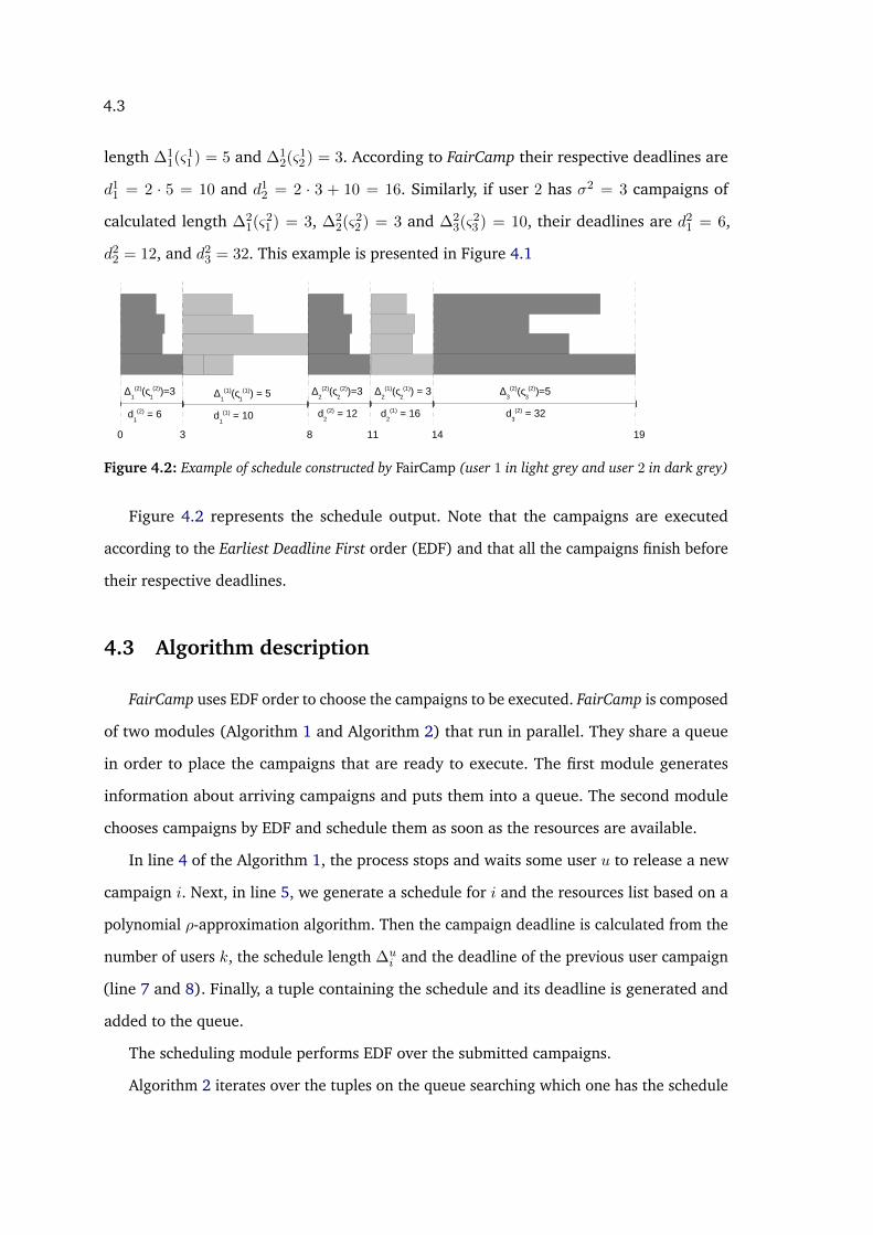
4.3

length ∆11(ς1

1 ) = 5 and ∆12(ς1

2 ) = 3. According to FairCamp their respective deadlines are

d11 = 2 · 5 = 10 and d1

2 = 2 · 3 + 10 = 16. Similarly, if user 2 has σ2 = 3 campaigns of

calculated length ∆21(ς2

1 ) = 3, ∆22(ς2

2 ) = 3 and ∆23(ς2

3 ) = 10, their deadlines are d21 = 6,

d22 = 12, and d2

3 = 32. This example is presented in Figure 4.1

Δ3

(2)(ς3(2))=5

d3

(2) = 32

Δ2

(1)(ς2(1)) = 3

d2

(1) = 16

Δ2

(2)(ς2(2))=3

d2

(2) = 12

Δ1

(1)(ς1

(1)) = 5

d1

(1) = 10

Δ1

(2)(ς1(2))=3

d1

(2) = 6

30 8 11 14 19

Figure 4.2: Example of schedule constructed by FairCamp (user 1 in light grey and user 2 in dark grey)

Figure 4.2 represents the schedule output. Note that the campaigns are executed

according to the Earliest Deadline First order (EDF) and that all the campaigns finish before

their respective deadlines.

4.3 Algorithm description

FairCamp uses EDF order to choose the campaigns to be executed. FairCamp is composed

of two modules (Algorithm 1 and Algorithm 2) that run in parallel. They share a queue

in order to place the campaigns that are ready to execute. The first module generates

information about arriving campaigns and puts them into a queue. The second module

chooses campaigns by EDF and schedule them as soon as the resources are available.

In line 4 of the Algorithm 1, the process stops and waits some user u to release a new

campaign i. Next, in line 5, we generate a schedule for i and the resources list based on a

polynomial ρ-approximation algorithm. Then the campaign deadline is calculated from the

number of users k, the schedule length ∆ui and the deadline of the previous user campaign

(line 7 and 8). Finally, a tuple containing the schedule and its deadline is generated and

added to the queue.

The scheduling module performs EDF over the submitted campaigns.

Algorithm 2 iterates over the tuples on the queue searching which one has the schedule

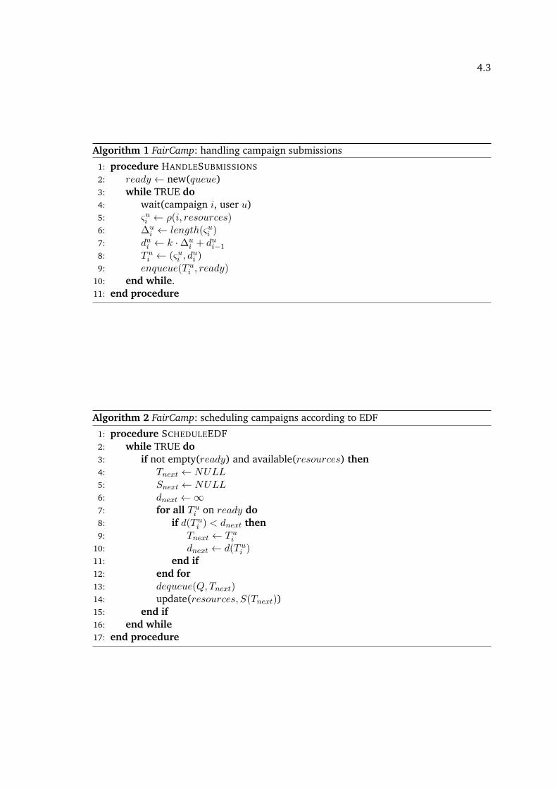
4.3

Algorithm 1 FairCamp: handling campaign submissions

1: procedure HANDLESUBMISSIONS

2: ready ← new(queue)3: while TRUE do4: wait(campaign i, user u)5: ςui ← ρ(i, resources)6: ∆u

i ← length(ςui )7: dui ← k ·∆u

i + dui−1

8: T ui ← (ςui , dui )

9: enqueue(T ui , ready)10: end while.11: end procedure

Algorithm 2 FairCamp: scheduling campaigns according to EDF

1: procedure SCHEDULEEDF2: while TRUE do3: if not empty(ready) and available(resources) then4: Tnext ← NULL5: Snext ← NULL6: dnext ←∞7: for all T ui on ready do8: if d(T ui ) < dnext then9: Tnext ← T ui

10: dnext ← d(T ui )11: end if12: end for13: dequeue(Q,Tnext)14: update(resources, S(Tnext))15: end if16: end while17: end procedure

4.4

with the lowest deadline (lines 7-12). In the end, the chosen campaign schedule is placed

on the resources (line 14).

4.4 Feasibility of FairCamp

FairCamp uses deadlines to guarantee fairness. Here, we show that a schedule produced

by FairCamp is always feasible, i.e., all the deadlines are met. First, we assume that a

campaign misses its deadline and then we show that this leads to a contradiction.

Proposition 4.1. In a schedule S produced by FairCamp, all campaigns finish their executions

before their respective deadlines.

Proof. Consider m processors and k users. For each campaign i, a schedule ςui is generated

whose length is ∆ui (ςui ). This length is calculated by a ρ-approximation algorithm using all

the processors. According to FairCamp, each campaign has deadline dui = k ·∆ui (ςui )+dui−1 =

k ·∆ui (ςui )+k ·∆u

i−1(ςui−1) . . . k ·∆u1(ςu1 ) = k ·

∑i ∆u

i (ςui ). This deadline states that the length

of each user workload can be stretched at a maximum factor of k. In other words, dui also

can be seen as the deadline of the partial workload (from the first campaign until campaign

i).

Now, consider a schedule S constructed by FairCamp where at least one campaign

misses its deadline and, without loss of generality, let campaign i from user u be the first

campaign to miss its deadline on S. By definition, dui = k ·∑

i ∆ui (ςui ), where

∑i ∆u

i (ςui ) is

the length of the (partial) workload issued from u.

Two conclusions can be observed from this scenario. First, the sum of the length of the

workloads issued from the other k− 1 users, between the beginning of the schedule (t = 0)

and the beginning of campaign i, is bigger than (k−1) ·∑

i ∆ui (ςui ). Otherwise, the schedule

would have an idle space, violating the campaign-compact constraint (Definition 3.1). All

the campaigns after this idle space (including campaign i) could be shifted to end before

dui . So, more formally,

4.5

•∑k

v 6=u∑σv

j ∆vj (ς

vj ) > (k − 1) ·

∑i ∆u

i (ςui ),

where σv is the number of campaigns on each partial workload.

Second, the deadline of each partial workload is equal to or less than the deadline of i.

More formally, ∀v 6= u:

• dvσv ≤ dui ;

• k ·∑σv

j ∆vj (ς

vj ) ≤ k ·

∑i ∆u

i (ςui );

• (k − 1) ·∑σv

j ∆vj (ς

vj ) ≤ (k − 1) ·

∑i ∆u

i (ςui ).

But this clearly contradicts the first conclusion.

4.5 Theoretical analysis

We analyze FairCamp from two perspectives. First, Corollary 4.1 shows that FairCamp

is efficient for an individual performance point of view, as∑

∆ui is increased by at most kρ

measured relatively to a system dedicated to the user. Second, Theorem 4.1 demonstrates

that FairCamp is fair, as it is a ρ-approximation for minimizing the maximum stretch over

all users.

Corollary 4.1. FairCamp is (kρ, . . . , kρ)-approximation for P |camp|∑

∆ui .

Proof. By definition, the length of a user workload execution is denoted by∑

∆ui . The dead-

line of a workload execution is the deadline of the last campaign duσu = k ·∑σu

i=1 ∆ui (ςui ) =

kρ ·∑σu

i=1 ∆u∗i , where

∑σu

i=1 ∆u∗i is the optimal length of the workload. Since all deadlines

are met, each workload is stretched by a factor of kρ, at maximum.

Theorem 4.1. FairCamp is ρ-approximation for max-stretch that does not depend on k.

4.5

Proof. Let us consider a solution S constructed by FairCamp for an instance of P |camp|∆ui .

Now, consider without loss of generality, that the first l scheduled campaigns belong to

user u while the campaign l+ 1 belongs to user v. Assume that sl is the start time and Cl is

completion time of campaign l. Similarly, sl+1 and Cl+1 are the start and completion time

of campaign l + 1. As campaign l + 1 starts immediately after campaign l, sl+1 = Cl. The

arrival time of campaigns l and l + 1 are tl = sl and tl+1 = 0, respectively.

As S was constructed by FairCamp, the deadline of l + 1 is larger or equal to the

deadline of l, otherwise, campaign l + 1 would be scheduled earlier (after one of the l first

campaigns). So, k ·∆vl+1(ςvl+1) ≥ k ·

∑l1 ∆u

i (ςui ). We also can denote this as Cl+1 − Cl ≥ Cl

or, more conveniently, Cl+1 ≥ 2Cl.

Regarding only these l + 1 campaigns, the stretch of user u is Du = Cl/∑l

1 ∆u∗i =∑l

1 ∆ui /∑l

1 ∆u∗i = ρ

∑l1 ∆u∗

i /∑l

1 ∆u∗i = ρ, while user v has Dv = (Cl+1 − tl+1)/∆v∗

l+1) =

ρ(Cl+1−tl+1)/(Cl+1−sl+1) = ρ(Cl+1)/(Cl+1−Cl). As (Cl+1)/(Cl+1−Cl) > 1, then Dv > ρ

and max(Du, Dv) = Dv.

Assume by contradiction that a better solution S′ is achieved by changing the positions

of campaigns l and l + 1. In this solution, the stretch of u is D′u = ρ(Cl+1 − sl)/(Cl − sl)

and the stretch of user v is D′v = ρ(Cl+1 − Cl + sl)/(Cl+1 − Cl). For this solution to be

better, both stretches of S′ should be lower than Dv:

• Dv > D′v

• ρ(Cl+1)/(Cl+1 − Cl) > ρ(Cl+1 − Cl + sl)/(Cl+1 − Cl)

• (Cl+1) > (Cl+1 − Cl + sl).

Since Cl + sl is positive, we proved that Dv > D′v. Now, for D′u:

• Dv > D′u

• ρ(Cl+1)/(Cl+1 − Cl) > ρ(Cl+1 − sl)/(Cl − sl)

• Cl+1(Cl − sl) > (Cl+1 − sl)(Cl+1 − Cl)

• Cl+1Cl − Cl+1sl > C2l+1 − Cl+1Cl − Cl+1sl + Clsl

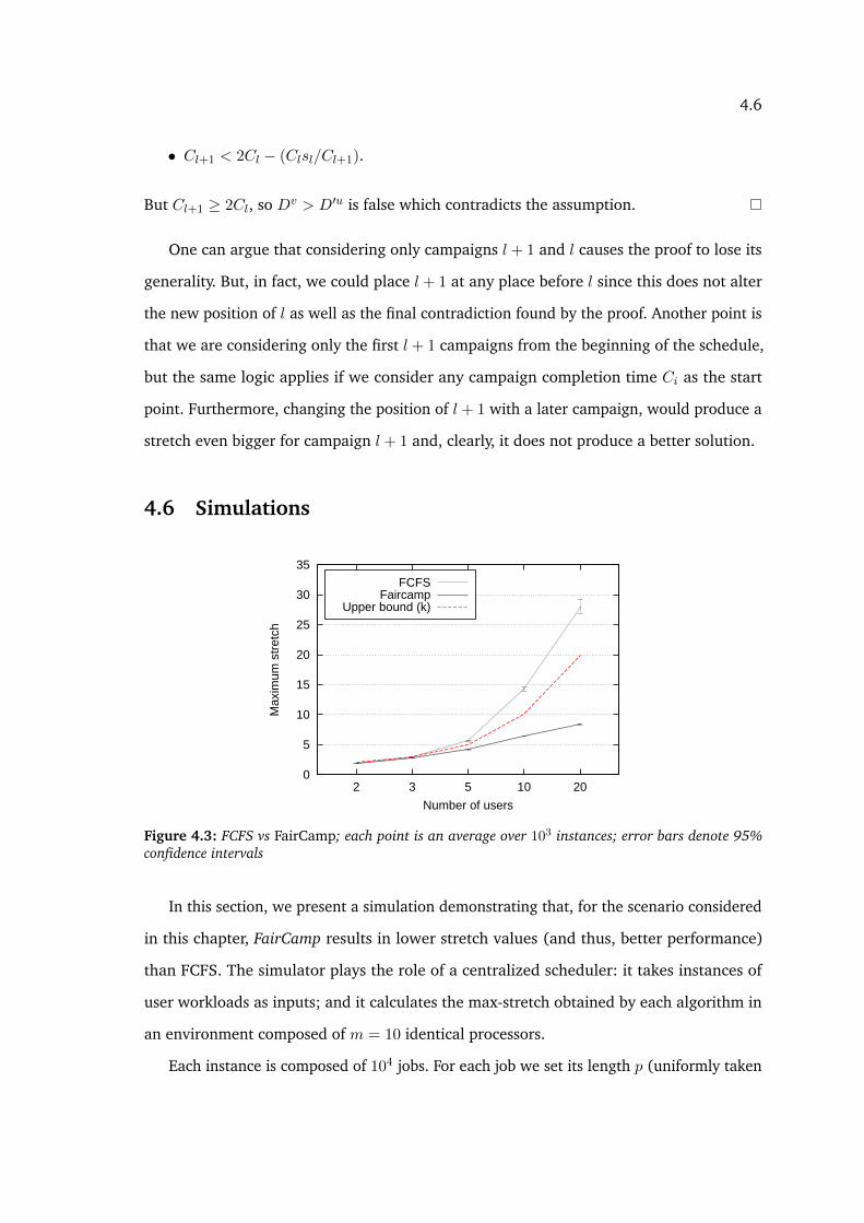
4.6

• Cl+1 < 2Cl − (Clsl/Cl+1).

But Cl+1 ≥ 2Cl, so Dv > D′u is false which contradicts the assumption.

One can argue that considering only campaigns l + 1 and l causes the proof to lose its

generality. But, in fact, we could place l + 1 at any place before l since this does not alter

the new position of l as well as the final contradiction found by the proof. Another point is

that we are considering only the first l + 1 campaigns from the beginning of the schedule,

but the same logic applies if we consider any campaign completion time Ci as the start

point. Furthermore, changing the position of l + 1 with a later campaign, would produce a

stretch even bigger for campaign l + 1 and, clearly, it does not produce a better solution.

4.6 Simulations

0

5

10

15

20

25

30

35

2 3 5 10 20

Ma

xim

um

str

etc

h

Number of users

FCFSFaircamp

Upper bound (k)

Figure 4.3: FCFS vs FairCamp; each point is an average over 103 instances; error bars denote 95%confidence intervals

In this section, we present a simulation demonstrating that, for the scenario considered

in this chapter, FairCamp results in lower stretch values (and thus, better performance)

than FCFS. The simulator plays the role of a centralized scheduler: it takes instances of

user workloads as inputs; and it calculates the max-stretch obtained by each algorithm in

an environment composed of m = 10 identical processors.

Each instance is composed of 104 jobs. For each job we set its length p (uniformly taken

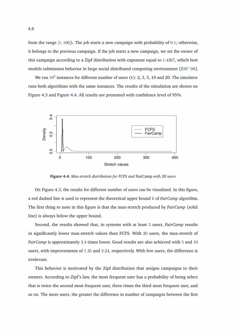
4.6

from the range [1, 100]). The job starts a new campaign with probability of 0.1; otherwise,

it belongs to the previous campaign. If the job starts a new campaign, we set the owner of

this campaign according to a Zipf distribution with exponent equal to 1.4267, which best

models submission behavior in large social distributed computing environment [IDE+06].

We run 103 instances for different number of users (k): 2, 3, 5, 10 and 20. The simulator

runs both algorithms with the same instances. The results of the simulation are shown on

Figure 4.3 and Figure 4.4. All results are presented with confidence level of 95%.

0 100 200 300 400

0.0

0.2

0.4

Stretch values

Den

sity FCFS

FairCamp

Figure 4.4: Max-stretch distribution for FCFS and FairCamp with 20 users

On Figure 4.3, the results for different number of users can be visualized. In this figure,

a red dashed line is used to represent the theoretical upper bound k of FairCamp algorithm.

The first thing to note in this figure is that the max-stretch produced by FairCamp (solid

line) is always below the upper bound.

Second, the results showed that, in systems with at least 5 users, FairCamp results

in significantly lower max-stretch values than FCFS. With 20 users, the max-stretch of

FairCamp is approximately 3.4 times lower. Good results are also achieved with 5 and 10

users, with improvements of 1.35 and 2.24, respectively. With few users, the difference is

irrelevant.

This behavior is motivated by the Zipf distribution that assigns campaigns to their

owners. According to Zipf’s law, the most frequent user has a probability of being select

that is twice the second most frequent user, three times the third most frequent user, and

so on. The more users, the greater the difference in number of campaigns between the first

4.6

user and the last one in the frequency rank. So, it is more likely that FCFS generates some

schedules that will affect users with few campaigns and, consequently, will result in high

values for the max-stretch.

Figure 4.4 is a density plot for the max-stretch values for FCFS and FairCamp with 20

users. For FairCamp all the max-stretch values falls between 5 and 13, the majority of them

being around 8. For FCFS the majority of instances produces max-stretch values between

10 and 50. Nonetheless, for some instances, the max-stretches are extremely high, some of

them reaching the hundreds. In fact, 7 of them fall between 100 and 400. This happens

because, despite its clear predominance around the average, FCFS is not bounded since it

does not take stretch into account, like FairCamp.

In the next chapter, a solution is proposed in order to fit a more wide and realistic

scenario. In this scenario users can join and leave the system (k is variable) and think-times

values are positive and arbitrary.

Chapter 5

Fair online schedules: dynamic

scenario

In real HPC systems, the number of users interacting with the resources is changing all

the time. Users log in, execute processes, wait for results and may log out at any moment.

Campaign submissions are unpredictable events as their executions are sparse, with idle

time intervals between them. With those unpredictable events taking place, the challenge

of delivering a fair scheduling is an even more complex endeavor, because the scheduler

needs to maintain fairness only among the users that are present at each time moment.

In this chapter, a new algorithm called OStrich is proposed to deal with this new, more

realistic, scenario. It follows the same principles of FairCamp, i.e., the fairness is achieved

by assigning due dates to each campaign and user performance is bounded by his/her own

workload and the number of users (although only “active” users are considered).

OStrich performance is assessed through simulating the replay of a workload trace from

a real cluster, whereas this trace is composed of sequential jobs. In order to understand

how to replay such traces, the simulations section is preceded by a discussion on how to

detect campaigns in workloads, including the job dependencies inside campaigns.

57

5.1

5.1 The OStrich online algorithm

The algorithm guarantees the worst-case stretch of each campaign (Dui ) to be propor-

tional to the campaign’s workload and the number of active users in the system. OStrich’s

principle is to create a virtual fair-sharing schedule that determines the execution priorities

of the campaigns in the real schedule. The algorithm maintains a list of ready-to-execute

campaigns ordered by their priorities and interactively selects the next job from the high-

est priority campaign. Any scheduling policy can be used to determine the execution

order of jobs within a single campaign; for instance LPT [Gra69] (or, more appropriately,

MLPT [Lee91]) or Shortest Processing Time (SPT) [BCS74].

The virtual fair-sharing schedule is maintained by dividing the processors between the

active users at each given moment. The processors are divided evenly among the users,

independently of users’ submitted workload. The priority of a user’s campaign is determined

by its virtual completion time, i.e. the completion time in the virtual schedule. The campaign

with the shortest virtual completion time has the highest priority for execution. This virtual

completion time of a campaign Jui is denoted by C̃ui (more generally, we will use x̃ for

denoting a variable x in the virtual schedule). That way, if a user u submits a campaign at

time tui , its virtual completion time is defined as the total workload of the campaign divided

by its share of processors, added by its virtual start time. More formally:

C̃ui (t) = W̃ ui /(m/k̃(t)) + s̃ui = k̃(t)W̃ u

i /m+ s̃ui . (5.1)

Note that the share of a user is defined as the number of processors m divided by

the number of active users at moment t, denoted by k̃(t). Active users are those users

that, according to the virtual schedule, have unfinished campaigns at time t. Formally, k̃(t)

is defined as k̃(t) =∑k

u 1{u, t} where 1{u, t} is an indicating function that returns 1 if

∃i | C̃ui > te and 0 otherwise.

A campaign starts in the virtual schedule after its submission, but also not sooner

than the virtual completion time of the previous campaign (the previous campaign can be

completed earlier in the real schedule than in the virtual schedule). Formally, the virtual

5.2

start time of a campaign is defined as

s̃ui = max(tui , C̃ui−1). (5.2)

This condition guarantees that at each time moment, at most one campaign of each user is

executing in the virtual schedule, as it happens on the real scheduler. Thus, the number of

allocated processors depends on the number of active users, regardless the system load.

Additionally, OStrich does not allow a campaign to start its execution before its virtual

start time (sui ≥ s̃ui ). This constraint keeps the real schedule in accordance with the fair

principles of the virtual schedule: a user should not be able to take a greater share of

the processors than what it was assigned in the virtual schedule. In other words, if a

campaign starts at s̃ui and finishes at C̃ui on the virtual schedule, during this time interval

its owner will not be able to execute jobs from another campaign. Furthermore, there is

no incentive for any of the users to lie about or hide their private information from the

other users. No advantage can be obtained by a user from splitting one campaign in many

single-job-campaigns and submitting them separately.

The virtual completion time of the campaigns can be updated on two events: the

submission of a new campaign and the completion of a campaign in the virtual schedule.

These events may change the number of active users (k̃(t)) and, by definition, the virtual

completion times of other active campaigns must also be modified.

Besides, at each event e occurring at time te, the virtual workload of a campaign (W̃ ui )

must be redefined based on how much it is left to be executed in the virtual schedule.

The remaining workload of a campaign is defined by taking the time passed since the last

event occurrence te−1 and multiplying it by the campaign’s share of processors on that time

interval. Considering all the events passed after the campaign’s submission, the workload

formula is W̃ ui =

∑j p

ui,j −

∑e(m.(te − te−1)/k̃(te−1)).

5.2

5.2 Example

Following, we have an example of how OStrich works. The Figure 5.1 shows the evolu-

tion of the real and the virtual schedule (labeled with ‘R’ and ‘V’ respectively) generated by

the OStrich algorithm from t = 0 to t = 18 in a system with 6 identical processors (labeled

from M1 to M6). This example shows 7 submissions issued from 3 different users: two

submissions at time t = 0 from users 1 and 2, two submissions at times t = 2 and t = 5

from user 3, one submission at t = 8 from user 2 and two submissions at t = 14 from users

2 and 3.

In the real schedule, each box represents the execution of a job wherein the box label

is the job length. In the virtual schedule, each box represents the load of a submitted

campaign wherein the box label represents the load in terms of processing time. Each time

the number of active users changes, the remaining workloads in the virtual schedule are

redistributed. A plus signal is used to indicate when the remaining load should be added to

the previous load in order to match the total campaign load. The list of ready campaigns

is also represented on the example. This list contains all the submitted campaigns sorted

accordingly to the owners priority. A callout is used to represent a campaign’s submission.

For a more didactic explanation of how OStrich works, the job executions are represented

by 6 subfigures, labeled from a to f . Also, each time a user campaign is finished, the

max-stretch value is updated, if necessary.

At t = 0 (a) the first campaigns of users 1 and 2 are submitted. From t = 0 to t = 2

(a and b), they are the only users in the system (k̃(t) = 2; 0 ≤ t ≤ 2). The virtual

schedule is constructed by sharing the processors equally between them and, according to

definition (5.1), their virtual completion times are C̃11 = 16 and C̃2

1 = 6. The real schedule

contains only jobs from user 2 since he/she has higher execution priority for having the

smallest virtual completion time.

5.2

10

M6

M5

M4

M3

M2

M1

M6M5

M4

M3

M2

M1

V

R

18

48

1 2 3

3

2

2

2

1

11

0

4

5

4

43

2

1 1

4

4

2

2

4

33

2

max-stretch

0.0

0.0

0.0V

R

2

3

3

2

2

6

6

2

2

+42

+12

1 1

113

2

2

1

1

1 4

5

4

432

1 1

4

422

4

33

2

max-stretch

0.0

0.0

0.0

M6

M5

M4

M3

M2

M1

M6

M5

M4

M3

M2

M1

V

R

12

3 53

2

2

1 1

1

4

3

2

2

1

1

1

6

6

2

5

10

+12

4

4

4

42

1

1

1 1

1

+42

4

3 3

2

1 1

22

321

8

max-stretch

0.0

1.6

1.0

M6

M5

M4

M3

M2

M1

M6

M5

M4

M3

M2

M1

V

R

12

3 53

2

2

1 1

1

4

3

2

2

1

1

1

6

6

2

8

10

+12

4

4

2

1

1

1 1

1

4

4

1 12

2

1

10

14

3 3

2 22

32

+42

2

21

8

max-stretch

0.0

1.6

1.0

M6

M5

M4

M3

M2

M1

M6

M5

M4

M3

M2

M1

V

R

12

3 53

2

2

1 1

1

4

3

2

2

1

1

1

6

6

2

10

+12

4

4

2

1

1

1

1

1

4

4

2

2

1

1

3

1 1

4

3

22

2

3

2

+18

6

2

2

8

1

+4

+4

+12

14

+9

21

1 2

8

1

1

8

21

1 2

1

1

max-stretch

0.0

2.0

3.0

M6

M5

M4

M3

M2

M1

M6

M5

M4

M3

M2

M1

V

R

12

3 53

2

2

1 1

1

4

3

2

2

1

1

1

6

6

2

10

+12

4

4

2

1

1

1

1

1

4

4

2

2

1

1

3

4

3

2

3

2

+18

6

2

2

8

1

+4

+4

+12

2

2

1

1

1

1

+9

8

8

1

1

2

2

2

1

1

2

1

1

max-stretch

2.375

2.0

3.0

M6

M5

M4

M3

M2

M1

M6

M5

M4

M3

M2

M1

List of ready campaigns List of ready campaigns

List of ready campaignsList of ready campaigns

List of ready campaigns List of ready campaigns

time time

time time

time time

a b

c d

e f

6 16

User 1

User 2

User 3

User 1

User 2

User 3

User 1

User 2

User 3

User 1

User 2

User 3

User 1

User 2

User 3

User 1

User 2

User 3

19

7 8 23

118 23 11 2313

18

Figure 5.1: An example of the virtual and real schedule generated by the OStrich algorithm with 3users

5.3

The situation changes at t = 2 when user 3 submits her/his first campaign (b). By

this time, the users 1 and 2 had each a share of 6 in the virtual schedule but their virtual

completion times were not exceeded. Now, the processors are equally shared between 3

users (k̃(2) = 3). The virtual completion time of user 3 is set to C̃31 = 7 and the virtual

completion times of users 1 and 2 are updated to C̃11 = 23 and C̃2

1 = 8, according to their

remaining workloads in the virtual schedule.

Still at t = 2, now, user 3 is the user with the highest priority. In the real schedule, the

first campaign of user 2 is interrupted and some jobs from user 3 starts. However, note that

the unfinished jobs from user 2 are not interrupted and so, in order to use processors M5

and M6, user 3 must wait until t = 3.

From t = 2 to t = 5 (b and c) the first campaign of user 3 is finished and also the first

campaign of user 2, as its remaining jobs are executed. Additionally, some jobs of the first

campaigns of user 1 finally start to execute. At t = 5 (c) the second campaign of user 3

is submitted, but note that the virtual completion time of her/his first campaign was not

exceeded yet (C̃31 = 7). So, as t32 < C̃3

1 and according to definition 5.2, s̃32 = C̃3

1 = 8. The

virtual completion time of this new campaign is set to 11 (C̃32 = 11).

The user 3 now has the highest priority but, following the start time constraint of

OStrich, her/his next campaign must wait until s̃32 to became eligible to be executed. So,

from t = 5 to t = 8 (c and d) only jobs from user 1 are executed. At t = 8 (d) the second

campaign of user 2 is submitted and its virtual completion time is set to 13. User 3 remains

having the highest priority and now his/her jobs start to be executed. From t = 8 to t = 14

(d and e) there are no new submissions, thus the already submitted campaigns of users 2

and 3, and some jobs of user 1, are executed accordingly to the priority order.

At t = 14 (e), the third campaigns from users 2 and 3 are submitted. Now, users 2

and 3 have equal priorities (and higher than that of user 3). The campaign 1 of user 3 is

interrupted and, from t = 14 to 18 (e and f), these new campaigns are executed, followed,

finally, for the remaining jobs of user 3.

Visually, the result of OStrich is a schedule with campaigns being interleaved and

executed in many pieces, according to the changing priorities between users.

5.3

5.3 Theoretical analysis

In this section, the worst case stretch of a campaign is analyzed. The idea for the proof is

to bound the completion time of the last job of a campaign using a “global area” argument

compared to the virtual schedule. In this proof, pmax denotes the maximum job length in

the system. “Area” is a measure in terms of amount of time × number of processors.

The virtual schedule is denoted by V and the real schedule by R. To simplify the

formulation of the proofs of this section, it is said that the virtual schedule V “executes an

area”, even though V is just an abstraction used for prioritizing real jobs. At time t, an area

is being “executed” by V if in V there is a fraction of processors assigned to this area.

5.3.1 Worst-case bound

As V can assign a job an arbitrary fraction of processors (from ε to m), a schedule in V

is represented by horizontal load streams, one for each active user. Idle intervals can be

present in V only when there are no ready jobs to be executed. In turn, R must execute

each job on a single processor, thus some processors can be idle even when there are ready

jobs. This can happen when tui < s̃ui and the ready jobs of campaign Jui must wait until

t = s̃ui . So, the question is whether the idle times that might additionally appear in R can

cause a systematic delay of R compared to V. The following lemma shows that once R is

delayed by an area of mpmax, the delay does not grow further, as there is always a ready

job to be executed.

The lemma considers only the idle time in the “middle” of the scheduling chart, i.e.,

after the start time of the first job and up to the start time of the last job; this is sufficient

to characterize the online behavior of OStrich.

Lemma 5.1. The total idle area in R (counted from the earliest to the latest job start time)

exceeds the total idle area in V by at most mpmax.

Proof. Consider first a V schedule with no idle times. Assume by contradiction that t is the

first time moment when the total idle area in R starts to exceed mpmax. Thus, at least one

processor is free at time t and there is no ready jobs to be executed. As V has no idle times,

5.3

at time t the area executed by V exceeds the area executed by R by more than mpmax. Thus,

the area exceeding mpmax is ready to be executed at R: as a single job has an area of at

most pmax, an area of mpmax is composed of at least m jobs. Thus, at least m jobs are being

executed, or ready to be executed in R at t. This contradicts the assumption that there is at

least one free processor in R at time t.

If there is idle time in V, it can be replaced by a set of dummy jobs JI that are “executed”

by V, but not necessarily (or not completely executed) by R. If R executes JI entirely, the

lemma is true, and this can be proved using the same argument of the previous paragraph,

since JI “contributes” with the same amount of idle area (∑pI) for V as well as for R. If R

executes JI partially (i.e. it executes a set J ′I , where 0 ≤ p′I ≤ pI), the contribution of these

jobs is smaller to the idle area of R than to the idle area of V (∑p′I ≤

∑pI).

R starts to execute jobs from campaign Jui when this campaign has the shortest com-

pletion time in V. Yet, it is possible that after some jobs from Jui have started, another

user v submits her/his campaign Jvj . If Jvj has a smaller area than what remains of Jui , it

gains a higher priority. In this case, Jui would be executed in R in so-called pieces: two jobs

Jk, Jl ∈ Jui belong to the same piece iff no job from other campaign Jvj starts between

them. That is, @J ′ : (J ∈ Jvj ) ∧ (sJk < sJ ′ < sJl).

The following lemma bounds the completion time of the last piece of the campaign.

After a campaign is completed in the virtual schedule, it cannot be delayed by any other

newly-submitted campaign; thus it has the highest priority and its remaining jobs are

executed in one piece (i.e., the last piece). The lemma upper-bounds the virtual area with

the higher priority by the area of the campaign, given that, in the worst case, k users submit

campaigns of equal area at the same time. In this case, they would end at the same time in

V and be executed in arbitrary order in R.

Lemma 5.2. The completion time Cui,q of the last piece q of a campaign Jui is bounded by a

sum:

Cui,q ≤ tui + kW ui−1

m+ pmax + (k − 1)

W ui

m+ pmax +

W ui

m+ pumax. (5.3)

Proof. In the expression (5.3), tui + kW ui−1/m expresses the maximum time a campaign

5.3

V(Virtual)

R(Real)

Cu

i-1

user u

timeCu

i,qsu

i,qS

tui

su

i

~Cu

i

~

Ju

i

... ... ...

Figure 5.2: Analysis of OStrich: bound for the campaign stretch

may wait until the virtual completion time of the previous campaign Jui−1 of the same user;

(k − 1)W ui /m bounds the time needed to execute other users’ campaigns that can have

higher priority; W ui /m + pumax bounds the execution time of the campaign Jui ; and two

pmax elements represent the maximum lateness of R compared to V and the maximum time

needed to claim all the processors.

From definitions (5.1) and (5.2), and knowing that tui ≥ s̃ui−1 (i.e. the next campaign

cannot be released before the previous one starts), we obtain s̃ui ≤ tui + kW ui−1/m.

There is no idle time in R in the period [s̃ui , sui,q), otherwise, the last piece could have

been started earlier. We denote by A the area of jobs executed in R after the time moment

s̃ui and until s̃ui,q. We claim that A ≤ mpmax + (k − 1)W ui +W ′ui , where W ′ui is the area of

jobs from campaign Jui executed until sui,q. The Figure 5.2 facilitates the visualization of

these notations, including the area A (shaded area).

To prove the claim, we analyze job J executed in R in the period [s̃ui , sui,q). First, J is

not executed in V after sui,q. If J were in V after sui,q, J would have lower priority than jobs

from campaign Jui , so OStrich would not choose J over jobs from campaign Jui .

Second, if J is executed in V before s̃ui , it means that R is “late” in terms of executed

area: but the total area of such “late” jobs it at most mpmax (from Lemma 5.1).

Thus, if J has a corresponding area in the virtual schedule executed in the period

[s̃ui , sui,q), the area A of the jobs started in the real schedule in this period is equal to the

5.3

area of the virtual schedule between [s̃ui , sui,q) plus the lateness mpmax. Recall that from

time sui,q till the start of the last job of Jui , the campaign Jui has the highest priority (as it is

not interrupted by any other campaign). Thus, at the latest, sui,q corresponds to the time

moment C̃ui in the virtual schedule when the campaign Jui completes (plus the lateness

pmax). By definition of the virtual schedule, sui,q ≤ pmax + s̃ui + kWu

im .

Starting from sui,q, the remaining jobs of Jui start and complete. Jui can claim all

processors at the latest pmax after sui,q. Then, by using classic lower bounds, it takes

W ui /m+ pumax to complete the campaign.

The following theorem states that in OStrich the stretch of a campaign depends only on

the number of active users and the relative area of two consecutive campaigns.

Theorem 5.1. The stretch of a campaign is proportional to the number of active users k1 and

the relative area of consecutive campaigns. Dui ∈ O(k(1 +

Wui−1

Wui

)).

Proof. The result follows directly from Lemma 5.2. Recall that, for campaign Jui , the stretch

Dui is defined by Du

i = (Cui − tui )/lui = (Cui − tui )/max(W ui /m, p

umax). Also, Cui = Cui,q,

i.e. the completion time of a campaign is equal to the completion time of its last “piece”.

Replacing Cui by the definition of Cui,q taken from Lemma 5.2, we have

Dui ≤

kWui−1m

+3pmax+kWu

im

max(Wui /m,p

umax) ≤

kWui−1m

+3pmax+kWu

im

Wui /m

≤ k(1 +Wu

i−1

Wui

) + 3mpmax.

For a given supercomputer, m is constant; similarly, the maximum size of a job pmax

can be treated as constant, as it is typically limited by system administrators. Hence,

Dui ∈ O(k(1 +W u

i−1/Wui )).

It is worth noting that the stretch does not depends on the current total load of the

system. Heavily-loaded users do not influence the stretch of less-loaded ones. Also, this

bound is tight as we will see next.1The number of active users may vary on time. Here, we assume that k is the biggest value it assumes

during the execution of the campaign.

5.4

5.3.2 Tightness

This section analyzes the tightness of the O(k(1 +Wu

i−1

Wui

)) bound proposed in Theo-

rem 5.1. We start with a negative result that says that in heavily-loaded systems, campaigns

have to be executed sequentially, thus at least one of them will have a stretch in O(k).

Proposition 5.1. No scheduling algorithm can achieve better stretch than O(k).

Proof. Consider an instance with k users, each submitting at t = 0 a campaign with m jobs

of unit size. The campaigns have to be executed sequentially, so there is at least one user

whose campaign completes at time k.

The following proposition shows an instance in which the bound O(k(1 +Wu

i−1

Wui

)) (The-

orem 5.1) is asymptotically tight. The instance is composed of a series of long campaigns

followed by a series of short campaigns. A user who had her/his long campaign executed

at the beginning, must wait with the short campaign not only the time needed to complete

all other long campaigns, but also possibly other short campaigns.

Proposition 5.2. The bound Dui ∈ O(k(1 +

Wui−1

Wui

)) is asymptotically tight.

Proof. Consider an instance with m processors and k users having two campaigns each. At

t = 0, each user submits a campaign with m jobs of size pmax. The second campaign of a

user is submitted immediately after the completion of the first campaign, with m jobs of

size p = 1. As campaigns {Ju1 } have the same priority; and campaigns {Ju2 } have the same

priority, OStrich can produce any schedule that executes first all the campaigns {Ju1 }, then

all campaigns {Ju2 }. Thus, an admissible schedule is (J11 , J

21 , . . . , J

(k)1 , J

(k)2 , J

(k−1)2 , . . . , J1

2 ).

The completion time of J12 is C1

2 = kpmax + k, thus the stretch D12 = (k − 1)pmax + k =

1 + (k − 1)(1 +W 1

1

W 12

).

5.4 Analysis of campaigns in workloads

In this section, we describe how to detect campaigns composed of sequential jobs in

workloads from real traces of production clusters.

5.4

5.4.1 Workload modeling

In recent works about workload modeling [Fei05, ZF12, MF12], Feitelson et al. consider

that the action of a user (i.e. his/her job submission behavior and frequency) is influenced

by the actions of the other users and by the scheduler decisions. This user feedback has an

impact on the observed workload.

This is justified by the fact that the user is aware of the current system behavior and

his future actions directly depend on the system’s actual performance. To incorporate this

feedback in the model, Feitelson proposes the postulate of dependencies between jobs,

which relies upon the idea of what he calls the think-time, i.e. the delay between the ending

of a job and the submission of a new one. This delay represents the time taken by the user

to analyze the result of a executed job and to prepare the submission of the next. This is

the same concept as the think-time in the Campaign Scheduling model.

In [ZF12], the think-time is used to detect user sessions and batches in a workload trace.

A user session is a period of continuous work where the user submits jobs. The continuity of

a session is defined by a time threshold. Interruption of user activities above this threshold

configures a session break. Within a session, jobs that are overlapping will be grouped in

what is called a batch. Note that, the notion of campaign is similar to the notion of batch: a

set of jobs, submitted asynchronously by a user and that will run independently from the

others.

Still on [ZF12], different methods are proposed to detect users’ batches in a workload

log. The LAST algorithm was originally proposed in [SF06]. In this approach, two jobs that

are submitted one after the other belong to the same batch if the last one was submitted

before the end of the first one. The ARRIVAL algorithm is based on the inter-arrival times of

the jobs, i.e. it does not take into account their runtimes. The MAX algorithm states that

a job belongs to a batch if it overlaps at least one of the jobs of the batch. According to

comparisons, the results showed that the choice of which algorithm should be adopted is

not general. The ARRIVAL algorithm, for example, is more adequate for web search engine

logs, as it was concluded at [MF12].

In this thesis, the MAX algorithm is adopted since it focus on task runtime and thus is

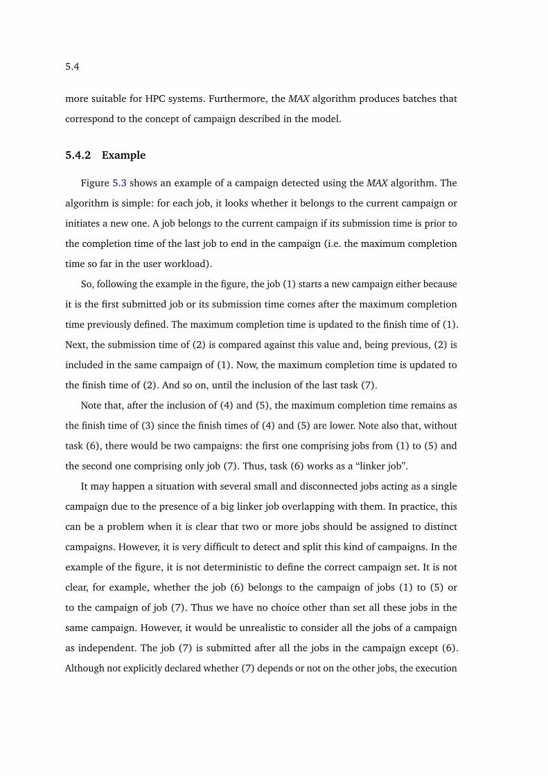
5.4

more suitable for HPC systems. Furthermore, the MAX algorithm produces batches that

correspond to the concept of campaign described in the model.

5.4.2 Example

Figure 5.3 shows an example of a campaign detected using the MAX algorithm. The

algorithm is simple: for each job, it looks whether it belongs to the current campaign or

initiates a new one. A job belongs to the current campaign if its submission time is prior to

the completion time of the last job to end in the campaign (i.e. the maximum completion

time so far in the user workload).

So, following the example in the figure, the job (1) starts a new campaign either because

it is the first submitted job or its submission time comes after the maximum completion

time previously defined. The maximum completion time is updated to the finish time of (1).

Next, the submission time of (2) is compared against this value and, being previous, (2) is

included in the same campaign of (1). Now, the maximum completion time is updated to

the finish time of (2). And so on, until the inclusion of the last task (7).

Note that, after the inclusion of (4) and (5), the maximum completion time remains as

the finish time of (3) since the finish times of (4) and (5) are lower. Note also that, without

task (6), there would be two campaigns: the first one comprising jobs from (1) to (5) and

the second one comprising only job (7). Thus, task (6) works as a “linker job”.

It may happen a situation with several small and disconnected jobs acting as a single

campaign due to the presence of a big linker job overlapping with them. In practice, this

can be a problem when it is clear that two or more jobs should be assigned to distinct

campaigns. However, it is very difficult to detect and split this kind of campaigns. In the

example of the figure, it is not deterministic to define the correct campaign set. It is not

clear, for example, whether the job (6) belongs to the campaign of jobs (1) to (5) or

to the campaign of job (7). Thus we have no choice other than set all these jobs in the

same campaign. However, it would be unrealistic to consider all the jobs of a campaign

as independent. The job (7) is submitted after all the jobs in the campaign except (6).

Although not explicitly declared whether (7) depends or not on the other jobs, the execution

5.4

order of jobs should be respected in order to define a worst-case assumption. We can solve

this by setting inter-job dependencies.

(1)

(2)

(3)

(4)

(5)

(6)

(7)

Figure 5.3: An example of a campaign with seven jobs according to the MAX algorithm

5.4.3 Interval graphs for job dependencies

The MAX algorithm is used to detect campaigns but not the internal job dependencies

inside campaigns. This can be done using interval graphs [Pap78] to describe the prece-

dence relations between jobs. Thus, for each campaign, we create an interval graph of all

the jobs that make up the campaign. In this graph, the jobs are the vertices and two vertices

are linked by an edge if the corresponding jobs overlap (between their submission time

and end time). Then, from this interval graph we build the dependency graph presented in

Figure 5.4. A job will have as dependencies all the jobs terminated before its submission.

Finally, we apply the transitive reduction on the dependency graph to remove transitive

edges.

(1)

(5)

(2)

(4)

(5)

(3)

(6)

(7)

Figure 5.4: A Directed Acyclic Graph (DAG) illustrating dependencies inside the campaign (samecampaign of Figure 5.3)

5.5

5.4.4 Campaigns with dependencies: a formal model

The former campaign model, introduced in Chapter 3, allowed to release any job of

a campaign when the campaign starts. Because of the way we detect campaigns (MAX

algorithm from [ZF12]), this induces a bias.

The MAX method, cannot guarantee that all the jobs in the campaign are overlapping.

In this case some jobs that stay in the system longer than the others behave as “linkers”

and group together in the same campaign jobs that do not run at the same time. Thus, in

the same campaign some jobs can start after another job’s termination. To guarantee that

we respect that constraint in the replay, we set up job dependencies during the campaign

detection. A job will have as dependencies all the jobs in the campaign terminated before

its submission.

OStrich can be extended to handle job dependencies: the jobs of a campaign are

primarily sorted by their number of immediate successors on decreasing order and secondly

by their length as in LPT [Gra69]. When a job is executed, it may trigger its successors to

become ready for execution. But if the highest priority campaign has no ready jobs, the

second highest priority campaign is chosen and so on.

5.5 Simulations

In this section, we analyze the performance of OStrich on a workload trace taken from a

real cluster machine. First, we describe the settings of the simulations and then we compare

the performance of OStrich to the standard scheduler (Maui with FCFS and backfilling)

used on this cluster.

To run the simulations, we choose the LPC-EGEE2 trace from the Parallel Workload

Archive [Fei] (cleaned version). This trace comes from a cluster that is part of the EGEE3

project and has the particularity of being composed of multiple Bag-of-Tasks (i.e. serial

jobs), which fits well the concept of a campaign. The scheduler used to produce the

execution trace was Maui [JSC01] with its default EASY configuration, that is, FCFS with2http://www.cs.huji.ac.il/labs/parallel/workload/l_lpc/index.html3http://public.eu-egee.org/intro/

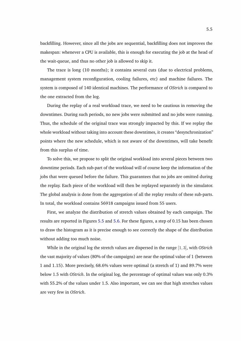
5.5

backfilling. However, since all the jobs are sequential, backfilling does not improves the

makespan: whenever a CPU is available, this is enough for executing the job at the head of

the wait-queue, and thus no other job is allowed to skip it.

The trace is long (10 months); it contains several cuts (due to electrical problems,

management system reconfiguration, cooling failures, etc) and machine failures. The

system is composed of 140 identical machines. The performance of OStrich is compared to

the one extracted from the log.

During the replay of a real workload trace, we need to be cautious in removing the

downtimes. During such periods, no new jobs were submitted and no jobs were running.

Thus, the schedule of the original trace was strongly impacted by this. If we replay the

whole workload without taking into account these downtimes, it creates “desynchronization”

points where the new schedule, which is not aware of the downtimes, will take benefit

from this surplus of time.

To solve this, we propose to split the original workload into several pieces between two

downtime periods. Each sub-part of the workload will of course keep the information of the

jobs that were queued before the failure. This guarantees that no jobs are omitted during

the replay. Each piece of the workload will then be replayed separately in the simulator.

The global analysis is done from the aggregation of all the replay results of these sub-parts.

In total, the workload contains 56918 campaigns issued from 55 users.

First, we analyze the distribution of stretch values obtained by each campaign. The

results are reported in Figures 5.5 and 5.6. For these figures, a step of 0.15 has been chosen

to draw the histogram as it is precise enough to see correctly the shape of the distribution

without adding too much noise.

While in the original log the stretch values are dispersed in the range [1, 3], with OStrich

the vast majority of values (80% of the campaigns) are near the optimal value of 1 (between

1 and 1.15). More precisely, 68.6% values were optimal (a stretch of 1) and 89.7% were

below 1.5 with OStrich. In the original log, the percentage of optimal values was only 0.3%

with 55.2% of the values under 1.5. Also important, we can see that high stretches values

are very few in OStrich.

5.5

0

10000

20000

30000

40000

1 2 3 4Stretch Value

Cou

nt

Figure 5.5: Campaign stretch values distribution (original log: Maui, FCFS)

Figures 5.7 and 5.8 show the system utilization, or the percentage of allocated resources

over time. The results of both algorithms look similar but it is worth to note that, with

OStrich, the system achieves its maximum utilization more often and more periods where

the system is empty are visible. This is interesting because OStrich maximizes the utilization

when there are jobs to process and thus creates periods of non-utilization of the platform

that can be used for Energy-Saving strategies, for example.

In order to obtain a more detailed look of the system utilization, we zoom into these

results (figures 5.9 and 5.10) to analyze an interval of two months (December and January).

These months were chosen due to their high rate of system utilization. The same observation

remains valid: with OStrich, peak usage activity is more frequent, and, unlike the original

log, it achieves 100% of resource utilization many times.

The precedence relations between jobs is obviously an obstacle to optimization: without

this, the level of parallelism would be higher and better stretch values could be obtained.

Thus, in theory, the absence of dependencies between jobs would increase system utilization.

The results in Figure 5.11 confirm this claim. This figure shows the system utilization of

the same period (December and January) in an OStrich schedule with no job dependencies.

In this scenario, the system utilization is more homogeneous. Regarding the periods where

the system load is above 10%, this scenario achieves system utilization at least 20% greater

5.5

0

10000

20000

30000

40000

1 2 3 4Stretch Value

Cou

nt

Figure 5.6: Campaign stretch values distribution (OStrich)

0

25

50

75

100

Oct Nov Dec Jan Feb Mar Apr MayDate

Sys

tem

Res

ourc

es A

lloca

tion

(%)

Figure 5.7: System resources utilization for whole trace (original log: Maui, FCFS)

than the one obtained with job dependencies. Not surprisingly, periods of user inactivity

are also more frequent.

The comparison of the two approaches of campaign detection, with and without adding

dependencies, is also interesting. Regarding the original workload shape, we can observe

that the replay with the no-dependencies approach is more biased. Whereas Figure 5.10 is

quite similar to Figure 5.9, Figure 5.11 shows a scenario where the utilization is better due

5.5

0

25

50

75

100

Oct Nov Dec Jan Feb Mar Apr MayDate

Sys

tem

Res

ourc

es A

lloca

tion

(%)

Figure 5.8: System resources utilization for the whole trace (OStrich)

0

25

50

75

100

Dec 01 Dec 15 Jan 01 Jan 15Date

Sys

tem

Res

ourc

es A

lloca

tion

(%)

Figure 5.9: System resources utilization for the extract (original log: Maui, FCFS)

to the arrival of jobs earlier in the campaigns. As the no-dependency approach does not

guarantee all the jobs precedence constraints from the original log, all the jobs can start at

the beginning of the campaign. Thus the workload is not really the same. Due to this, we

recommend the dependencies detection approach when making performance comparison

between the replay output and the original log. It guarantees that user behavior and system

5.5

0

25

50

75

100

Dec 01 Dec 15 Jan 01 Jan 15Date

Sys

tem

Res

ourc

es A

lloca

tion

(%)

Figure 5.10: System resources utilization for the extract (OStrich, with job dependencies)

0

25

50

75

100

Dec 01 Dec 15 Jan 01 Jan 15Date

Sys

tem

Res

ourc

es A

lloca

tion

(%)

Figure 5.11: System resources utilization for the extract (OStrich, no dependencies)

utilization are consistent with the original output.

Now, we present another simulation to demonstrates how OStrich and FCFS react to

different user profiles, concerning the job length that is preferably submitted by each

profile. The simulator plays the role of a centralized scheduler: it takes an instance of a user

workload a input, and it calculates the campaign stretches and the max-stretch per user

5.5

0

1000

2000

3000

4000

1−2 2−4 4−6 6−8 8−10 10−12 12−14 14−16 16−18 18−20 over 20Stretch Interval

Cam

paig

n C

ount

AlgorithmFCFSOstrich

Figure 5.12: Ostrich vs FCFS: stretch values by intervals

obtained by each algorithm in an environment composed of m = 64 identical processors.

Due to the difficulty to find a real log with well defined user profiles, and in order to

provide a better control of the experiment, we use a synthetic workload trace, generated to

model two different user profiles.

We run 40 instances where instance is composed of 104 jobs. For each job we set its

length p according to the user profile. We defined 2 user profiles: short-job profile and

long-job profile. Short-job users submit short jobs with lengths uniformly taken from the

range [1; 3.6 × 103] (seconds as time unit). Long-job users submit long jobs with lengths

uniformly taken from the range [3.6× 103; 3.6× 104]. Each job starts a new campaign with

probability of 0.02; otherwise, it belongs to the previous campaign. If the job starts a new

campaign, we set the owner of this campaign according to a uniform distribution.

In general, the results confirm our expectations and show that OStrich results in

significantly lower max stretches than FCFS. The Figure 5.12 shows the distribution of

stretch values for all campaigns. The number of campaigns with stretch lower than 2 for

OStrich is more than twice the number obtained with FCFS. More important, though is

the number of high stretch values above: while on OStrich this number decreases rapidly

towards 0 as stretch increases, with FCFS it is bigger than 2600 above 20, representing

5.5

1

10

Short LongUser Job length profile

Max

Str

etch

Mea

n

Algorithm

Ostrich

FCFS

Figure 5.13: Ostrich vs FCFS: max campaign stretch mean per user profile

42.3% of the total. The occurrence of stretch values above 20 is only 117 for OStrich (1.3%).

The Figure 5.13 shows the max stretch average per user profile (in a log scale) and here

we can see how OStrich accomplishes its purpose: short users are penalized by FCFS with

big stretch values (whose average is above 50) while OStrich does not heavily discriminate

users by their profiles, guaranteeing a more fair treatment for all the users (average of

12.8 for short users). For long users, FCFS and OStrich have almost the same performance

(average of 6.3 for FCFS and 6.8 for OStrich).

In the next chapter, the OStrich is extended in order to handle parallel jobs. This

extension manages the virtual schedule in a different way than when scheduling sequential

jobs. The virtual schedule is modified like a malleable job, taking only the number of used

processors to avoid priority inconsistencies.

Chapter 6

Scheduling parallel jobs with

OStrich

The study of sequential job scheduling is useful for optimizing the execution of

embarrassingly parallel applications. These applications follow the Bag-of-Tasks (BoT)

model [LSV06, CM10], with no communication requirements. However, despite the ap-

plicability of this model, many scientific applications are composed of parallel jobs that

need to be executed concurrently in order to synchronize the communication between their

tasks and improve their performance.

In this chapter, the OStrich algorithm presented before is adapted to handle parallel

jobs of type rigid. The theoretical analysis is updated accordingly and it shows that user

performance is still bounded by his/her own workload and the number of active users. On

the other hand, in this new setting the stretch also depends on the maximum utilization

rate of the system (i.e. the maximum number of machines a parallel job is allowed to

require).

6.1 Parallel OStrich

When dealing with parallel jobs, OStrich behavior is slightly different from the sequential

job version. Now, the campaigns are executed following a greedy approach that strives to

79

6.1

�������

���

�

�

���

���������������������

�

�

���

���������������������

�

�

���

���������������������

�

�

���

���������������������

�����

�����

�����

Figure 6.1: Delay problem between real and virtual schedule

keep all the machines occupied. The virtual and real schedule roles remain unaltered: the

virtual schedule builds an ideal fair allocation of resources from which the priorities of

the campaigns are derived and it is updated in an event driven fashion. The real schedule

determines how the jobs are scheduled according to these priorities. But there are some

changes concerned to the way the virtual schedule is build.

6.1.1 Event based resizing

In parallel job scheduling, it can not be guaranteed that all the machines will be

occupied. Because of that, the delay between the real and virtual schedule is not bounded

by a fixed amount as it was for sequential jobs. (in Chapter 5 it was proved that, for

sequential jobs, the delay was bounded by a fixed amount). This can lead to a situation

where campaigns start to be executed after their virtual completion times, resulting in

wrong priority assignments.

In the Figure 6.1, an example with 3 users is given to illustrate how this might occur

when the sequential version of OStrich is used to schedule parallel jobs. This example shows

the evolution of the real and the virtual schedule in a system with m identical processors.

The users are identified by different shades of gray (dark, medium, and light gray). A

dotted line is used to represent the present moment during the schedule, the dashed area

represents idle processor time and a dashed line is used on the real schedule to split the

6.2

�

�

����

�����������������������

�

�

����

�����������������������

�

�

����

�����������������������

�

�

����

�����������������������

�����

�����

�����

�������

����

�����

Figure 6.2: Delay correction using a resized virtual schedule

resources in two equal sets.

This example shows that the virtual schedule is computed using all the machines,

regardless of the number of idle processors in the real schedule. The first two campaigns

(from gray and dark gray users) are scheduled correctly. The third campaign (from the light

gray user) arrives just after the virtual completion time of the dark gray user is achieved,

so the higher priority remains with the dark gray user until his/her campaign finishes.

However, the second campaign of the gray user arrives before the virtual completion time of

the light gray user. The problem is that, despite having a very small workload, the campaign

of the gray user must wait for the execution of the light gray campaign that has a higher

priority and is still in the queue of ready campaigns. The conclusion is that using all the

resources to compute the virtual schedule favors users that use less resources in situations

of low utilization.

To tackle this issue, the virtual schedule must be resized to take into account the amount

of idle processors on the real schedule. Figure 6.2 shows a corrected version of the same

example, according to a resized virtual schedule.

More precisely, when an event occurs, the algorithm counts the number of idle proces-

sors between the present moment and the moment of the previous event. Then, it reduces

the number of available processors in the virtual schedule during this time interval to be

the same as in the real schedule. Then, the completion times are recomputed accordingly.

6.2

6.2 Algorithm description

Algorithm 3 The OStrich algorithm

1: procedure OSTRICH

2: idle_procs← {M1,M2, ...,Mm}3: for each new event E do4: last_event← curr_event5: curr_event← E6: interval← time(curr_event) - time(last_event)7: resize(virtual, users, interval, size(idle_procs))8: if curr_event is SUBMISSION then9: Jui ← extract campaign from curr_event

10: insert Jui on Q11: insert u on users12: update(virtual, users)13: execute(Q, idle_procs, priorities(virtual))14: end if15: if curr_event is JOB_FINISHED then16: Jui ← extract job from curr_event17: insert procs used by Jui,j on idle_procs18: execute(Q, idle_procs, priorities(virtual))19: end if20: if curr_event is VIRTUAL_CAMP_FINISHED then21: Jui ← extract campaign from curr_event22: if Jui is last submitted by u then23: remove u from users24: end if25: update(virtual, users)26: end if27: end for28: end procedure

First, in the beginning of the scheduler, the set of idle processors contains all the

machines, as none of the resources are being used (line 2).

Inside the for loop, the algorithm waits for the next event (line 3) and when it happens,

the virtual schedule is resized to not take into account the resources that were idle between

the present event and the previous one (line 7). This resize function is also responsible for

recomputing the campaigns virtual completion times. The three types of events that are

handled by the algorithm are campaign submissions (line 8), job completions (line 15) and

virtual completion time of campaigns (line 20).

When a campaign is submitted, it is put on the list of ready jobs represented by Q

6.3

(line 10) and the user is added to the set of active users (line 11). The virtual schedule is

updated to reset the virtual completion times and the scheduler proceeds the execution

with an asynchronous call (lines 12 and 13). That way, after the call, the execution flow

goes back and waits for another event to happen.

The execute function called in lines 13 and 18 executes the campaigns according to the

following greedy algorithm:

1. Look at the current amount of machines available;

2. Find the first job in the queue of ready campaigns that fits on these available machines

and schedule it on these machines;

3. Remove these machines from the set of idle processors;

4. Repeat this process until there are no more jobs to schedule.

Inside the queue, the jobs of the campaigns are ordered according to LJF (Largest-Job-

First) [LC91], that is, according to job’s size (qui,j) in non-increasing order. This technique

has been proven to lead to higher utilization than SJF (Shortest-Job-First) and FCFS [Aid00,

HL10].

When a job finishes, the processors that were allocated to it are freed (line 2) and the

scheduler proceeds the execution in the same manner as in the paragraph above.

Finally, when the virtual completion time of a campaign is reached, its owner is removed

from the list of active users and the virtual schedule is updated (line 23). But this happens

only if this campaign is the last one submitted by the user. Otherwise, the user will remain

active, given that this campaign will be followed by another campaign.

6.3 Example

The Figure 6.3 shows the evolution of the real and the virtual schedules generated

by OStrich from t = 0 to t = 7 in a system with 5 identical processors. This example

shows 3 submissions issued from 3 different users identified by shades of gray (dark,

medium and light gray). The size and the length of each job is indicated in a label with

6.4

�������

���

��

��

��

��

��

��

� �

���

�����

��

��

��

��

���

���

���

��� ���

�������

���

��

��

��

��

��

��

�

���

�����

��

��

��

��

���

��

��� ���

�������

���

��

��

��

��

��

� ���

� ���

���

�����

��

��

��

��

���

��

���

���

���

���������������������� ���������������������� ����������������������

����

Figure 6.3: Virtual and real schedule generated by the OStrich algorithm with 3 users

a format. A dotted line is used to represent the present moment during

the schedule and the dashed area represents idle processor time.

At time t = 0, two campaigns from distinct users are submitted. At this point, the virtual

schedule is constructed taking into account all the machines and the medium gray user has

the higher priority. At time t = 5 the first jobs finish and, following this event, the virtual

schedule is resized to take into account only the number of used processors. Since there

are no more jobs from the medium gray user, the dark gray user is the next on the priority

list and its first job is selected for execution. Finally, at t = 7, the light gray user submits

its first campaign. Following this new submission, the virtual schedule is updated onward

and the light gray user gets the higher priority. However, note that he/she will have to wait

until t = 11, when the executing dark gray job finishes. Still at this moment, the virtual

schedule is resized again, taking the number of used processors since the last event.

6.4 Comparison with existing scheduling strategies

In this section, we use an example with parallel jobs to compare OStrich with space

sharing and FCFS (First-Come-First-Served). The purpose is to show how OStrich can offer

a solution that, while following a space sharing strategy, makes a more wise use of the

6.4

�

�� � ����

Figure 6.4: FCFS example with 2 users

system through a time sharing based execution that improves the stretch experience of

users.

In this example, the loads are 2 campaigns, each one issued by a different user, submitted

at the same moment on the beginning of the schedule. The users are represented by two

shades of gray and the optimal lengths for the campaigns are x and 1 for the light gray and

dark gray user, respectively.

FCFS executes jobs according to their order of arrival. It is a classical and widely used

strategy, because it is very simple to understand and to implement, and jobs do not starve.

However, it is well known that, for stretch optimization, FCFS can be arbitrarily far from

the optimal as illustrated in Figure 6.4. In this figure, the light gray campaign obtains an

optimal stretch. But the dark gray campaign obtains a stretch of x, that corresponds to the

length of the light gray campaign. Stretch, in this case, depends on the load submitted by

other users.

Space share is a common strategy used by actual systems to provide fairness between

users. In fairshare the users are given the same share of resources. However, this results in

6.4

�

�� ����

���

Figure 6.5: Space share example with 2 users

a very poor performance for the users since they can only use just the amount of resources

relative to their shares. Therefore, this strategy inherently strives to give a stretch of k for

all the users (where k is the number of active users). Another disadvantage is that, large

jobs cannot be executed if their sizes exceed the owner share. They would wait until the

user quota increases, which is not guaranteed to happen.

Figure 6.5 shows the same situation as before, now with campaigns being scheduled by

the fairshare algorithm. We can see that, from the beginning of the schedule, the resources

are divided by 2 and the first jobs are scheduled within these shares. The gray user jobs are

executed in sequence because there is not enough share to execute them in parallel. This

causes the dark gray campaign stretch to be 3, with the light gray campaign stretch being

x+ 3.

OStrich also provides fairness between users but it uses the fairshare strategy just to give

priorities to the user campaigns, leaving the execution in charge of a greedy algorithm. The

users with the higher priority have their jobs executed first and can use all the machines.

Figure 6.6 shows how the same input of the earlier examples are handled by OStrich.

In this case, along with the real schedule there is a virtual fairshare schedule that gives

the higher priority to the dark gray campaign. It is executed first by the greedy algorithm,

6.5

�

�����

�

��

��

�

�

Figure 6.6: OStrich example with 2 users

followed by the light gray campaign. In this case, the dark gray campaign stretch is optimal.

The light gray campaign stretch is x+ 1 and, although not optimal, is still better than the

one obtained with fairshare.

6.5 Theoretical analysis

In this section we bound the worst case stretch of a campaign in Parallel OStrich. The

idea of the main proof is to bound the completion time of the last job of a campaign using

a “conservative space” argument between the real and the virtual schedule. The “space” is

6.5

a measure in terms of amount of time × number of processors.

In the proofs outlined in this section, pmax denotes the maximum job length in the

system and α is the maximum utilization rate allowed per job where α ∈ [0, 1]. So, αm is

the maximum job size. The virtual schedule is denoted by V and the real schedule by R. To

simplify the formulation of proofs, we say that the virtual schedule V “executes” jobs even

though V is just an abstraction used for defining the priority of real jobs. At time t, a job is

“executed” by V if in V there is a fraction of processors assigned to this job.

6.5.1 Worst-case bound

First, we will prove that maximum number of idle processors in R is a function of α.

Lemma 6.1. At any time t, if |Q| 6= ∅, then at most αm processors are idle on R, where Q is

the queue of ready jobs.

Proof. Consider a schedule S constructed by OStrich. Let us assume by contradiction that

at some time t the number of idle processors is bigger than αm and |Q| 6= ∅. Now, consider

J as the first job started after t. So, as J has size at maximum αm and J ∈ Q at moment t,

then J could be scheduled earlier at time t. So, the schedule S was not constructed by a

greedy algorithm. But this is a contradiction since OStrich is greedy.

Now, we prove that the idle space in R is the same represented in V .

Lemma 6.2. The idle space on V is equal to the idle space on R for any time interval [ti, ti+1].

Proof. In the real schedule, the number of idle processors can be changed only at two

events. The first one is when a job is done. When this happens, the processors that were

allocated to this job are freed and become idle. The second event is when a new campaign

is submitted, causing idle processors to be allocated to new jobs. These two events are

represented in the Algorithm 3. In this same algorithm, between any two events, the virtual

schedule will always be adjusted, i.e., the same idle space present in R, between the two

events, will also be inserted to V.

6.5

Corollary, from this lemma: since V and R have the same number of machines, the

amount of space in R used to execute jobs between a time interval [ti, ti+1] is the same in

V .

Lemma 6.3. The completion time Cui,q of the last piece q of a campaign Jui is bounded by a

sum:

Cui,q ≤ tui +

kW ui−1

m+

(k − 1)W ui

m+W ui

m(1− α) + pmax

(6.1)

Proof. For the first part of this proof, let us consider as if all the m machines were used all

the time during the schedule. The part kW ui−1/m corresponds to the maximum time the

previous campaign of the same user can take to execute and so, the campaign Jui must wait

this time at maximum to be able to start its execution. The part (k − 1)W ui /m expresses

the maximum time that takes to execute all the campaigns with higher priorities than Jui .

Finally, W ui /m+ pmax bounds the maximum time that takes to execute Jui .

Using all the machines, the executed area between s̃ui and C̃ui is at most (C̃ui − s̃ui )m.

However, according to Lemma 1, the idle space between s̃ui and C̃ui can be at most

(C̃ui − s̃ui )αm and, so, the executed area can be (C̃ui − s̃ui )(1 − α)m in the worst case.

Hence, the stretch of any campaign within the executed area will be at most ((C̃ui −

s̃ui )m)/((C̃ui − s̃ui )(1− α)m) = 1/(1− α).

Finally, regarding pmax, the campaign can finish in the real schedule after its completion

on the virtual schedule (C̃ui ). However, according to Lemma 2, the idle (and executed)

spaces of R and V are equal for the same time interval. From this, we conclude that if

the last part of Jui is beyond C̃ui by an exceeding area S, it means that an equal area S′

composed of lower priority jobs were executed before C̃ui . But the interval Cui − C̃ui can not

be bigger than pmax, otherwise one or more jobs from Jui would have to be started in S,

even having a higher priority than the ones represented by S′. But this is a contradiction.

The Figure 6.7 illustrates the notations used in this proof and can be used to facilitate

the comprehension.

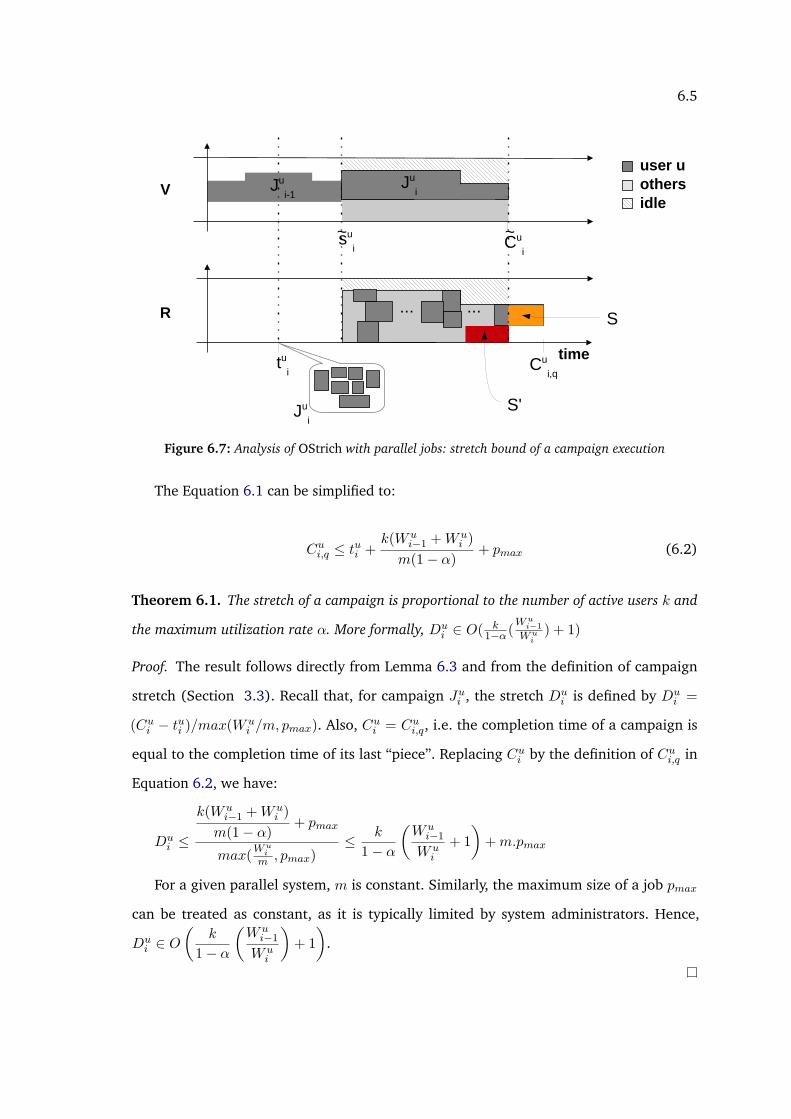
6.5

�

�

������

�����

���

�

���

��

�

��

�

��

�

��� ���

������

��

���

��

���

���

Figure 6.7: Analysis of OStrich with parallel jobs: stretch bound of a campaign execution

The Equation 6.1 can be simplified to:

Cui,q ≤ tui +

k(W ui−1 +W u

i )

m(1− α)+ pmax (6.2)

Theorem 6.1. The stretch of a campaign is proportional to the number of active users k and

the maximum utilization rate α. More formally, Dui ∈ O( k

1−α(Wu

i−1

Wui) + 1)

Proof. The result follows directly from Lemma 6.3 and from the definition of campaign

stretch (Section 3.3). Recall that, for campaign Jui , the stretch Du

i is defined by Dui =

(Cui − tui )/max(W u

i /m, pmax). Also, Cui = Cu

i,q, i.e. the completion time of a campaign is

equal to the completion time of its last “piece”. Replacing Cui by the definition of Cu

i,q in

Equation 6.2, we have:

Dui ≤

k(W ui−1 +W u

i )

m(1− α)+ pmax

max(Wu

im , pmax)

≤ k

1− α

(W u

i−1

W ui

+ 1

)+m.pmax

For a given parallel system, m is constant. Similarly, the maximum size of a job pmax

can be treated as constant, as it is typically limited by system administrators. Hence,

Dui ∈ O

(k

1− α

(W u

i−1

W ui

)+ 1

).

Chapter 7

Conclusion and ongoing work

The popularization of parallel systems leveraged by the emergence of low cost desktop

platforms like clusters, grids and, more recently, clouds promotes the emergence of new

user profiles and applications, whose needs impose new challenges for the HPC community,

particularly on the field of scheduling theory. In the last decades, the fair division of

resources has attracted the attention of scientists from many areas such as mathematics,

physics, economics and computer science. Nevertheless, existing theoretical models did not

capture all the dynamics involved in real environments.

In this thesis, we study fairness in multi-user parallel systems over different settings to

provide solutions where all users feel satisfied about the way resources are shared among

them. In order to model submissions issued by many users over time, we define and use

the Campaign model where each user submits campaigns of jobs in an interactive manner.

We provide an algorithm that schedules the resources among users in a fair way without

compromising system and individual performances. Among all the techniques available to

achieve fairness, the stretch metric was chosen because it measures the responsiveness of

the system taking into account each user expectation.

The solutions presented in this thesis propose a compromise between fairness and

individual performance for different Campaign Scheduling scenarios. These solutions are

implemented as online scheduling algorithms that explicitly maintain fairness among users

by bounding the worst-case stretch of each campaign whereas the stretch is defined by

91

7.1

means of a function derived from the campaign’s response time. It is shown that the

performance experienced by a user does not depend on the total load of the system, but

only on his/her submissions’ loads and on the number of users competing for the processors.

Furthermore, in some cases, the performance of each user can be optimized.

More specifically, we can conclude that:

• it is possible to maintain fairness among users in an online fashion, with bounded

performance. The solutions proposed in this thesis, specially OStrich and parallel

OStrich, are suitable fair solutions to be considered since they deliver theoretical

performances that are better than actual fair schedulers .

• According to the analysis and simulations presented throughout this thesis, fair

scheduling is necessary in order to provide responsiveness, specially in heavy loaded

systems, on which the discrepancy between the solutions proposed and actual solu-

tions achieve is bigger.

OStrich works with the premise that job processing times are known in advance as

opposite to the majority of actual system schedulers. In practice, even when processing time

estimates are requested from the user, the real processing times can be radically different.

In fact, most actual systems as Slurm [YJG03] and OAR [CDCG+05] handle this issue by

punishing users who make bad predictions that causes misuse of resources. OStrich can

also be adapted to handle user punishment. As an example, the ratio between predicted

processing time and real processing time could be used to adjust the user share in the

virtual schedule causing changes in the priorities. In this thesis, we chose to not tackle this

subject because it is a complementary mechanism. It can be used to adjust the priorities

but it is not relevant as the fairness per se.

7.1 Work contributions and perspectives

This thesis contributes in both theoretical and practical sides. From the theoretical point-

of-view, it presents algorithms that allows a fair scheduling in a multi-user parallel system

under realistic assumptions, along with models, definitions, lemmas, theorems and proofs

7.1

that sustain these capabilities. From the practical point-of-view, it provides a campaign

scheduling simulator and the results provided by it. The simulator code is available at https:

//forge.imag.fr/frs/download.php/568/cssim.zip, but before downloading, an account

must be created at https://forge.imag.fr/account/register.php.

These contributions were organized and published at international events. In December

2012, the campaign model and the FairCamp algorithm were published in the annual IEEE

International Conference on High Performance Computing (HiPC 2012), held in Pune,

India. In September 2013, the OStrich algorithm was published in the 10th International

Conference on Parallel Processing and Applied Mathematics (PPAM 2013), held in Warsaw,

Poland.

Below, the publications with more detailed information.

• Campaign Scheduling. Vinicius Pinheiro, Krzysztof Rzadca and Denis Trystram. The

IEEE International Conference on High Performance Computing (HiPC), pages 1-10.

Pune, India, December 2012.

• OStrich: Fair Scheduling For Multiple Submissions. Joseph Emeras, Vinicius Pinheiro,

Krzysztof Rzadca and Denis Trystram. The International Conference on Parallel

Processing and Applied Mathematics (PPAM 2013). LNCS. Springer, 2013.

• Fair Scheduling for Multiple Submissions. Joseph Emeras, Vinicius Pinheiro, Krzysztof

Rzadca and Denis Trystram. Tech Report. Université de Grenoble, June 2012.

I also co-authored a paper along with professors Krzysztof Rzadca and Denis Trystram on

the 10th conference on “New Challenges in Scheduling Theory”, held in Frejus, France, in

October 2012. The paper was entitled “Fairness Between Users in the Campaign Scheduling

Problem”.

Still, focusing on Parallel OStrich, we submitted a paper with the most recent results

entitled “Online Fair Scheduling of Burst Submissions of Parallel Jobs” to the 27th IEEE

International Parallel & Distributed Processing Symposium (IPDPS 2014) that will be held

on May 2014 in Phoenix, USA.

As future directions, we plan to analyze the Campaign Scheduling problem and the

solutions provided in this thesis under the light of game theory. More specifically, we plan

to study the envy-freeness property and if it can be guaranteed by the algorithms that were

proposed in this work.

Further, we plan to relax the campaign scheduling model to be more general, including

campaign execution overlapping. We also plan to analyze the behavior of OStrich in a

general multi-user scheduling problem, with users submitting single and independent jobs

instead of whole campaigns and the analysis being towards the max-stretch of individual

jobs.

In the practical side, we plan to do experiments with OStrich in a production system

with real users and compare it to SLURM. In order to perform this, the first step is already

done given that an implementation of OStrich is recently available at https://github.com/

filipjs/OStrich, as a plugin for the SLURM resource manager .

Special acknowledgment

This work was supported by the French-Polish bilateral cooperation program “Polonium”

and by the CAPES/COFECUB program (project number 4971/11-6). The PhD candidate

held part of his studies at University of Grenoble, from October 2011 to September 2012,

under the terms of a co-supervision scholarship between the University of São Paulo and

the University of Grenoble.

Bibliography

[Ada65] J Stacy Adams. Inequity in social exchange. Advances in experimental social

psychology, 2(267-299), 1965. 3

[Aid00] Kento Aida. Effect of job size characteristics on job scheduling performance.

Em DrorG. Feitelson e Larry Rudolph, editors, Job Scheduling Strategies for

Parallel Processing, volume 1911 of Lecture Notes in Computer Science, páginas

1–17. Springer Berlin Heidelberg, 2000. 83

[AMPP04] Alessandro Agnetis, Pitu B. Mirchandani, Dario Pacciarelli e Andrea Paci-

fici. Scheduling problems with two competing agents. Operations Research,

52(2):229–242, 2004. 17

[And04] D. P. Anderson. Boinc: a system for public-resource computing and storage.

Em Grid Computing, 2004. Proceedings. Fifth IEEE/ACM International Workshop

on, páginas 4 – 10, nov. 2004. 2, 33

[BCM98] Michael A. Bender, Soumen Chakrabarti e S. Muthukrishnan. Flow and

stretch metrics for scheduling continuous job streams. Em Proceedings of the

ninth annual ACM-SIAM symposium on Discrete algorithms, SODA ’98, páginas

270–279, Philadelphia, PA, USA, 1998. Society for Industrial and Applied

Mathematics. 24, 37, 44

[BCS74] J. Bruno, Jr. E. G. Coffman e R. Sethi. Scheduling independent tasks to reduce

mean finishing time. Commun. ACM, 17(7):382–387, Julho 1974. 15, 25, 58

[BK] Peter Brucker e Sigrid Knust. Complexity results for scheduling problems.

95

http://www.informatik.uni-osnabrueck.de/knust/class/. Last accessed on 19

Sep, 2012. 2, 11, 12

[BMR02] Michael A. Bender, S. Muthukrishnan e Rajmohan Rajaraman. Improved

algorithms for stretch scheduling. Em Proceedings of the thirteenth annual

ACM-SIAM symposium on Discrete algorithms, SODA ’02, páginas 762–771,

Philadelphia, PA, USA, 2002. Society for Industrial and Applied Mathematics.

24

[BTEP00] Jacek Blazewicz, Denis Trystram, Klaus Ecker e Brigitte Plateau. Handbook on

parallel and distributed processing. Springer-Verlag New York, Inc., 2000. 1,

10

[CDCG+05] Nicolas Capit, Georges Da Costa, Yiannis Georgiou, Guillaume Huard, Cyrille

Martin, Grégory Mounié, Pierre Neyron e Olivier Richard. A batch scheduler

with high level components. Em Cluster Computing and the Grid, 2005. CCGrid

2005. IEEE International Symposium on, volume 2, páginas 776–783. IEEE,

2005. 26, 92

[CDS10] H. Casanova, F. Desprez e F. Suter. Minimizing stretch and makespan of

multiple parallel task graphs via malleable allocations. Em Parallel Processing

(ICPP), 2010 39th International Conference on, páginas 71 –80, sept. 2010. 24

[CM10] Javier Celaya e Loris Marchal. A fair decentralized scheduler for bag-of-tasks

applications on desktop grids. Em Cluster, Cloud and Grid Computing (CCGrid),

2010 10th IEEE/ACM International Conference on, páginas 538 –541, may

2010. 21, 24, 79

[DLG11] Bruno Donassolo, Arnaud Legrand e Cláudio Geyer. Non-cooperative schedul-

ing considered harmful in collaborative volunteer computing environments.

Em Proceedings of the 2011 11th IEEE/ACM International Symposium on Cluster,

Cloud and Grid Computing, CCGRID ’11, páginas 144–153, Washington, DC,

USA, 2011. IEEE Computer Society. 3

[Dro09] M. Drozdowski. Scheduling for Parallel Processing. Computer Communications

and Networks. Springer, 2009. 21, 30

[ER06] Stephen Emmott e Stuart Rison. Towards 2020 science. Relatório técnico,

Working Group Reserach. Microsoft Research Cambridge, 2006. 1

[Fei] Dror G. Feitelson. Parallel workload archive. http://www.cs.huji.ac.il/labs/

parallel/workload/. Last accessed on 28 Sep, 2012. 71

[Fei05] Dror Feitelson. Workload Modeling for Computer Systems Performance Evalua-

tion. 2005. 68

[Geo10] Yiannis Georgiou. Contributions for Resource and Job Management in High

Performance Computing. Tese de Doutorado, Université de Grenoble, France,

2010. Supervisor - Olivier Richard; Co-supervisor - Jean François Méhaut. 27

[GLLK79] R. L. Graham, E. L. Lawler, J. K. Lenstra e A. H. G. Rinnooy Kan. Optimization

and approximation in deterministic sequencing and scheduling: a survey.

Em E.L. Johnson P.L. Hammer e B.H. Korte, editors, Discrete Optimization II

Proceedings of the Advanced Research Institute on Discrete Optimization and

Systems Applications of the Systems Science Panel of NATO and of the Discrete

Optimization Symposium co-sponsored by IBM Canada and SIAM Banff, Aha.

and Vancouver, volume 5 of Annals of Discrete Mathematics, páginas 287 – 326.

Elsevier, 1979. 11, 37

[Gra66] R. L. Graham. Bounds for certain multiprocessing anomalies. Bell System

Technical Journal, 45:1563–1581, 1966. 12

[Gra69] R. L. Graham. Bounds on multiprocessing timing anomalies. SIAM JOURNAL

ON APPLIED MATHEMATICS, 17(2):416–429, 1969. 14, 25, 58, 71

[GS58] G. Gamow e M. Stern. Puzzle-math. Macmillan, 1958. 4

[Hen95] Robert L Henderson. Job scheduling under the portable batch system. Em Job

scheduling strategies for parallel processing, páginas 279–294. Springer, 1995.

26

[HL10] Hsiu-Jy Ho e Wei-Ming Lin. Task scheduling for multiprocessor systems with

autonomous performance-optimizing control. J. Inf. Sci. Eng., 26(2):347–361,

2010. 83

[Hoo05] Han Hoogeveen. Multicriteria scheduling. European Journal of Operational

Research, páginas 592–623, 2005. 16

[HS87] Dorit S. Hochbaum e David B. Shmoys. Using dual approximation algorithms

for scheduling problems theoretical and practical results. J. ACM, 34:144–162,

January 1987. 20

[IDE+06] Alexandru Iosup, Catalin Dumitrescu, Dick Epema, Hui Li e Lex Wolters. How

are real grids used? the analysis of four grid traces and its implications. Em

Proceedings of the 7th IEEE/ACM International Conference on Grid Computing,

GRID ’06, páginas 262–269, Washington, DC, USA, 2006. IEEE Computer

Society. 55

[IPC+09] Michael Isard, Vijayan Prabhakaran, Jon Currey, Udi Wieder, Kunal Talwar e

Andrew Goldberg. Quincy: fair scheduling for distributed computing clusters.

Em Proceedings of the ACM SIGOPS 22nd symposium on Operating systems

principles, SOSP ’09, páginas 261–276, New York, NY, USA, 2009. ACM. 21

[JSC01] David B. Jackson, Quinn Snell e Mark J. Clement. Core algorithms of the

maui scheduler. Em Revised Papers from the 7th International Workshop on

Job Scheduling Strategies for Parallel Processing, JSSPP ’01, páginas 87–102,

London, UK, UK, 2001. Springer-Verlag. 27, 71

[KPS13] Ian Kash, Ariel D. Procaccia e Nisarg Shah. No agent left behind: dynamic

fair division of multiple resources. Em Proceedings of the 2013 international

conference on Autonomous agents and multi-agent systems, AAMAS ’13, páginas

351–358, Richland, SC, 2013. International Foundation for Autonomous

Agents and Multiagent Systems. 21

[KSS+05] Rajkumar Kettimuthu, Vijay Subramani, Srividya Srinivasan, Thiagaraja Gopal-

samy, D. K. Panda e P. Sadayappan. Selective preemption strategies for parallel

job scheduling. Int. J. High Perform. Comput. Netw., 3(2/3):122–152, Novem-

bro 2005. 47

[LC91] Keqin Li e Kam-Hoi Cheng. Job scheduling in a partitionable mesh using a

two-dimensional buddy system partitioning scheme. Parallel and Distributed

Systems, IEEE Transactions on, 2(4):413–422, 1991. 83

[Lee91] Chung-Yee Lee. Parallel machines scheduling with nonsimultaneous machine

available time. Discrete Appl. Math., 30:53–61, January 1991. 58

[LKB77] Jan Karel Lenstra, AHG Rinnooy Kan e Peter Brucker. Complexity of machine

scheduling problems. 1977. 11, 12

[LSV06] Arnaud Legrand, Alan Su e Frédéric Vivien. Minimizing the stretch when

scheduling flows of biological requests. Em Proceedings of the eighteenth

annual ACM symposium on Parallelism in algorithms and architectures, SPAA

’06, páginas 103–112, New York, NY, USA, 2006. ACM. 24, 79

[MF12] David Mehrzadi e Dror G. Feitelson. On extracting session data from activity

logs. Em Proceedings of the 5th Annual International Systems and Storage

Conference, SYSTOR ’12, páginas 3:1–3:7, New York, NY, USA, 2012. ACM. 68

[Pap78] C.H. Papadimitriou. Scheduling Interval-ordered Tasks. TR // Center for

Research in Computing Technology, Harvard University. Center for Research

in Computing Techn., Aiken Computation Laboratory, Univ., 1978. 70

[Pro13] Ariel D. Procaccia. Cake cutting: not just child’s play. Commun. ACM, 56(7):78–

87, Julho 2013. 4, 21

[PRT12] Vinicius Pinheiro, Krzysztof Rzadca e Denis Trystram. Campaign scheduling.

Em IEEE International Conference on High Performance Computing (HiPC),

Proceedings, páginas 1–10, 2012. 38

[RLAI04] David Raz, Hanoch Levy e Benjamin Avi-Itzhak. A resource-allocation queue-

ing fairness measure. SIGMETRICS Perform. Eval. Rev., 32(1):130–141, Junho

2004. 21, 27

[SF06] E. Shmueli e D.G. Feitelson. Using site-level modeling to evaluate the perfor-

mance of parallel system schedulers. Em Modeling, Analysis, and Simulation of

Computer and Telecommunication Systems, 2006. MASCOTS 2006. 14th IEEE

International Symposium on, páginas 167 – 178, sept. 2006. 68

[Sit] TOP500 Supercomputer Sites. Development over time. http://www.top500.

org/statistics/overtime/. Last accessed on 30 Aug, 2013. 1

[SKS04] Gerald Sabin, Garima Kochhar e P. Sadayappan. Job fairness in non-

preemptive job scheduling. Em Proceedings of the 2004 International Confer-

ence on Parallel Processing, ICPP ’04, páginas 186–194, Washington, DC, USA,

2004. IEEE Computer Society. 21, 27

[SKSS02] S. Srinivasan, R. Kettimuthu, V. Subramani e P. Sadayappan. Characterization

of backfilling strategies for parallel job scheduling. Em Parallel Processing

Workshops, 2002. Proceedings. International Conference on, páginas 514–519,

2002. 27

[SLL+49] Samuel A Stouffer, Arthur A Lumsdaine, Marion Harper Lumsdaine, Robin M

Williams Jr, M Brewster Smith, Irving L Janis, Shirley A Star e Leonard S

Cottrell Jr. The american soldier: combat and its aftermath.(studies in social

psychology in world war ii, vol. 2.). 1949. 3

[SS05] Gerald Sabin e P. Sadayappan. Unfairness metrics for space-sharing parallel

job schedulers. Em Proceedings of the 11th international conference on Job

Scheduling Strategies for Parallel Processing, JSSPP’05, páginas 238–256, Berlin,

Heidelberg, 2005. Springer-Verlag. 21, 44

[ST09] Erik Saule e Denis Trystram. Multi-users scheduling in parallel systems. Em

Proc. of IEEE International Parallel and Distributed Processing Symposium 2009,

páginas 1–9, Washington, DC, USA, may 2009. 17, 18, 19, 20, 38, 42

[Try12] Denis Trystram. Les riches heures de l’ordonnancement. TSI (Revue des sciences

et technologies de línformation), 31(8-10):1021–1047, 2012. 12

[Ull75] J. D. Ullman. Np-complete scheduling problems. J. Comput. Syst. Sci.,

10(3):384–393, Junho 1975. 12

[Val90] Leslie G. Valiant. A bridging model for parallel computation. Commun. ACM,

33(8):103–111, 1990. 33

[VC05] Sangsuree Vasupongayya e Su-Hui Chiang. On job fairness in non-preemptive

parallel job scheduling. Em IASTED PDCS, páginas 100–105, 2005. 21

[Voo03] Mark Voorneveld. Characterization of pareto dominance. Operations Research

Letters, 31:7–11, january 2003. 16

[WC01] Yiqiong Wu e Guohong Cao. Stretch-optimal scheduling for on-demand data

broadcasts. Em Computer Communications and Networks, 2001. Proceedings.

Tenth International Conference on, páginas 500 –504, 2001. 24

[YJG03] AndyB. Yoo, MorrisA. Jette e Mark Grondona. Slurm: Simple linux util-

ity for resource management. Em Dror Feitelson, Larry Rudolph e Uwe

Schwiegelshohn, editors, Job Scheduling Strategies for Parallel Processing, vol-

ume 2862 of Lecture Notes in Computer Science, páginas 44–60. Springer Berlin

Heidelberg, 2003. 26, 27, 92

[Zah] Matei Zaharia. The hadoop fair scheduler. http://hadoop.apache.org/docs/

r1.1.2/fair_scheduler.html. Last accessed on 22 April, 2012. 27

[ZAT05] Julia Zilber, Ofer Amit e David Talby. What is worth learning from parallel

workloads?: a user and session based analysis. Em Proceedings of the 19th

annual international conference on Supercomputing, ICS ’05, páginas 377–386,

New York, NY, USA, 2005. ACM. 5

[ZF12] Netanel Zakay e Dror G. Feitelson. On identifying user session boundaries

in parallel workload logs. Em Proc. of the 16th Workshop on Job Scheduling

Strategies for Parallel Processing, The Hebrew University, Israel, may 2012. 5,

68, 71