The Making of the Modern Metropolis:Evidence from London∗

Stephan Heblich†

University of Bristol

Stephen J. Redding‡

Princeton University, NBER and CEPR

Daniel M. Sturm§

London School of Economics and CEPR

September 20, 2017

Abstract

Modern metropolitan areas involve large concentrations of economic activity and the transport of millions of

people each day between their residence and workplace. However, relatively little is known about the role of these

commuting �ows in promoting agglomeration forces. We use the revolution in transport technology from the inven-

tion of steam railways, newly-constructed spatially-disaggregated data for London from 1801-1921, and a quantitative

urban model to provide evidence on the determinants of the concentration of economic activity in metropolitan areas.

Steam railways dramatically reduced travel times and hence permitted the �rst large-scale separation of workplace

and residence to realize economies of scale. We show that our model is able to account both qualitatively and quan-

titatively for the observed changes in city size, structure and land prices.

KEYWORDS: agglomeration, urbanization, transportation,

JEL CLASSIFICATION: O18, R12, R40

Work in Progress

∗We are grateful to Bristol University, the London School of Economics, and Princeton University for research support. We are grateful to

colleagues for helpful comments. We would like to thank the Cambridge Group for the History of Population and Social Structure, the British

Library and London Metropolitan Archives (LMA) for their help with data. We are grateful to Iain Bamford, Dennis Egger, Andreas Ferrara, Ben

Glaeser and Florian Trouvain for excellent research assistance. The usual disclaimer applies.

†Dept. Economics, Priory Road Complex, Priory Road, Clifton, BS8 1TU. UK. Tel: 44 117 3317910. Email: stephan.heblich@bristol.ac.uk.

‡Dept. Economics and WWS, Fisher Hall, Princeton, NJ 08544. Tel: 1 609 258 4016. Email: reddings@princeton.edu.

§Dept. Economics, Houghton Street, London, WC2A 2AE. UK. Tel: 44 20 7955 752. Email: d.m.sturm@lse.ac.uk.

1

1 Introduction

Modern metropolitan areas include vast concentrations of economic activity, with Greater London and New York

City today accounting for around 8.4 and 8.5 million people respectively. These immense population concentrations

involve the transport of millions of people each day between their residence and workplace. Today, the London

Underground alone handles around 3.5 million passenger journeys per day, and its trains travel around 76 million

kilometers each year (about 200 times the distance between the earth and the moon). Yet relatively little is known

about the role of these commuting �ows in promoting the agglomeration forces that sustain metropolitan areas. On

the one hand, these commuting �ows impose substantial real resource costs, both in terms of time spent commuting

and the construction of large networks of complex transportation infrastructure. On the other hand, they are also

central to creating dense employment concentrations to realize economies of scale in business districts and foster the

amenities available in distinctively residential neighborhoods.

In this paper, we use the mid-nineteenth century transport revolution from the invention of steam railways, a

newly-created, spatially-disaggregated dataset for Greater London from 1801-1921, and a quantitative urban model

to provide new evidence on the determinants of agglomeration. The key idea behind our approach is that the slow

travel times achievable by human or horse power implied that most people lived close to where they worked when

these were the main modes of transportation. In contrast, the invention of steam railways dramatically reduced the

time taken to travel a given distance, thereby permitting the �rst large-scale separation of workplace and residence.

This specialization by workplace and residence in turn enabled the realization of economies of scale in production and

residential choices. Using both reduced-form and structural approaches, we �nd substantial e�ects of steam passenger

railways on city size and structure. We show that our model is able to account both qualitatively and quantitatively

for the observed changes in city size, structure and land prices.

Methodologically, we develop a new structural estimation procedure for the class of urban models characterized

by a gravity equation for commuting �ows. Although we only observe these bilateral commuting �ows in 1921 at the

end of our sample period, we show how this framework can be used to estimate the impact of the construction of the

railway network. Combining our 1921 gravity equation data with historical information on population, land values

and the transport network back to the early-nineteenth century, we use the model to infer missing employment work-

place for each location going backwards in time. In overidenti�cation checks, we compare these model predictions to

the historical data on employment by workplace that do exist for the City of London. We �nd substantial direct e�ects

of the railway through reduced commuting costs, but we also �nd substantial changes in the relative productivity and

amenities of di�erent locations within Greater London, which are consistent with agglomeration forces in production

and residential choices.

Nineteenth-century London is arguably the poster child for the large metropolitan areas observed around the

world today. In 1801, London’s built-up area housed around 1 million people and spanned only 5 miles East to West.

This was a walkable city of 60 squares and 8,000 streets that was not radically di�erent from other large cities from

history. In contrast, by 1901, Greater London contained over 6.5 million people, measured more than 17 miles across,

and was on a dramatically larger scale than any previous urban area. This was the largest city in the world by some

margin (with New York City and Greater Paris having populations of 3.4 million and 4 million respectively at the

2

turn of the twentieth century) and London’s population exceeded that of several European countries.1

Therefore,

nineteenth-century London provides a natural testing ground for assessing the empirical relevance of theoretical

models of city size and structure.

Our empirical setting also has a number of other attractive features. During this period, there is a revolution in

transport technology in the form of the steam locomotive, which was initially developed to haul freight at mines

(at the Stockton to Darlington Railway in 1825), and only later applied to passenger transport (with the London and

Greenwich Railway in 1836 the �rst to be built speci�cally for passengers).2

In contrast to other cities such as Paris,

London developed through a largely haphazard and organic process. Until the creation of the Metropolitan Board

of Works (MBW) in 1855, there was no municipal authority that spanned the many di�erent local jurisdictions that

made up Greater London, and the MBW’s responsibilities were largely centered on infrastructure. Only in 1889 was

the London County Council (LCC) created, and the �rst steps towards large-scale urban planning for Greater London

were not taken until the Barlow Commission of 1940. Therefore, nineteenth-century London provides a setting in

which we would expect both the size and structure of the city to respond to decentralized market forces.

We contribute to several strands of existing research. First, our paper connects with the theoretical and empirical

literatures on agglomeration, including Henderson (1974), Fujita, Krugman, and Venables (1999), Fujita and Thisse

(2002), Davis and Weinstein (2002), Davis and Dingel (2012) and Kline and Moretti (2014), as reviewed in Rosenthal

and Strange (2004), Duranton and Puga (2004), Moretti (2011) and Combes and Gobillon (2015). A key challenge in em-

pirical work on agglomeration is �nding exogenous sources of variation to identify agglomeration forces. Rosenthal

and Strange (2008) and Combes, Duranton, Gobillon, and Roux (2010) use geology as an instrument for population

density, exploiting the idea that tall buildings are easier to construct where solid bedrock is accessible. Greenstone,

Hornbeck, and Moretti (2010) provide evidence on agglomeration spillovers by comparing changes in total factor pro-

ductivity (TFP) among incumbent plants in “winning” counties that attracted a large manufacturing plant and “losing”

counties that were the new plant’s runner-up choice. In contrast, we exploit the transformation of the relationship

between travel time and distance provided by the invention of the steam locomotive.

Second, our paper is related to a recent body of research on quantitative spatial models, including Allen and

Arkolakis (2014), Ahlfeldt, Redding, Sturm, and Wolf (2015), Redding and Sturm (2008), Redding (2016), Monte (2016),

Caliendo, Parro, Rossi-Hansberg, and Sarte (2017), Desmet, Nagy, and Rossi-Hansberg (2017), Allen, Arkolakis, and Li

(2017) and Monte, Redding, and Rossi-Hansberg (2017), as reviewed in Redding and Rossi-Hansberg (2017). All of these

papers focus on time period for which modern transformation networks by rail and/or road existed, whereas we exploit

the dramatic change in transport technology provided by the steam locomotive. We borrow our basic model structure

from Ahlfeldt, Redding, Sturm, and Wolf (2015), which introduces heterogeneity in worker commuting decisions

following McFadden (1974) into the urban model of Lucas and Rossi-Hansberg (2002). Our main methodological

contribution is to develop a new structural estimation procedure for quantitative urban models of this form that

feature a gravity equation for commuting �ows. This structural estimation procedure uses bilateral commuting �ows

for a baseline year (in our case 1921) and estimates the model’s parameters by undertaking comparative statics from

this baseline year (in our case backwards in time).3

We show that this procedure can be used to recover unobserved

1London overtook Beijing’s population in the 1820s, and remained the world’s largest city until the mid-1920s, when it was eclipsed by New

York. By comparison, Greece’s 1907 population was 2.6 million, and Denmark’s 1901 population was 2.4 million.

2Stationary steam engines have a longer history, dating back at least to Thomas Newcomen in 1712, as discussed further below.

3In Ahlfeldt, Redding, Sturm, and Wolf (2015), only data on a random sample of bilateral commuting �ows were available, which were not

3

historical employment by workplace (prior to 1921) from the bilateral commuting data for our baseline year and

historical data on population and land rents. This procedure is applicable in other contexts, in which historical data

are incomplete or missing, but bilateral commuting data are available for a baseline year.

Third, our paper is related to a growing empirical literature on the relationship between the spatial distribution

of economic activity and transport infrastructure, as reviewed in Redding and Turner (2015). One strand of this

literature has used variation across cities and regions, including Duranton and Turner (2011), Chandra and Thompson

(2000), Duranton and Turner (2012), Faber (2014), Michaels (2008), Donaldson (2017), Duranton, Morrow, and Turner

(2014), and Baum-Snow, Henderson, Turner, Zhang, and Brandt (2017). A second strand of this literature has looked

within cities, including Warner (1978), Jackson (1987), McDonald and Osuji (1995), Gibbons and Machin (2005), Baum-

Snow and Kahn (2005), Billings (2011), Brooks and Lutz (2013), and Gonzalez-Navarro and Turner (2016). Within this

literature, our work is most closely related to research on suburbanization and decentralization, including Baum-

Snow (2007), Baum-Snow, Brandt, Henderson, Turner, and Zhang (2017), and Baum-Snow (2017). Our contributions

are again to use the large-scale variation from the transition from human/horse power to steam locomotion and to

show that our model can account both qualitatively and quantitatively for the observed changes in city structure.

The remainder of the paper is structured as follows. Section 2 discusses the historical background. Section 3

summarizes the data sources and de�nitions. Section 4 presents reduced-form evidence on the role of transport in-

frastructure improvements in shaping patterns of urban development within Greater London. Section 5 introduces

our theoretical model. Section 6 undertakes a quantitative analysis of the model centered around its gravity equation

predictions for bilateral commuting �ows. Section 7 concludes.

2 Historical Background

London has a long history of settlement that dates back to before the Roman Conquest of England in 43 CE. We dis-

tinguish four main de�nitions of its geographical boundaries, which we now list from largest to smallest, where each

subsequent region is a subset of the previous one. First, we consider London together with the Home Counties that

surround it, which contain a 1921 population of 9.61 million and an area of 12,829 kilometers squared, and encompass

large parts of South-East England.4

Second, we examine Greater London, as de�ned by the modern boundaries of the

Greater London Authority (GLA), which includes a 1921 population of 7.39 million and an area of 1,595 kilometers

squared. Third, we consider the historical County of London, which has a 1921 population of 4.48 million and an area

of 314 kilometers squared. Fourth, we examine the City of London, which has a 1921 population of 13,709 and an

area of around 3 kilometers squared, and whose boundaries correspond approximately to the Roman city wall. From

medieval times, the City of London acted as the main commercial and �nancial center of what became the United

Kingdom, with the neighboring City of Westminster serving as the seat of Royal and Parliamentary government.5

Data are available for these four main geographical regions at two main levels of spatial aggregation: boroughs

and parishes. The Home Counties including Greater London encompasses 257 boroughs and 1,161 parishes; Greater

London contains 99 boroughs and 285 parishes; the County of London comprises 29 boroughs and 184 parishes; and

the City of London includes 1 borough and 111 parishes.6

In Figure 1, we show the outer boundary of the Home

representative for each workplace and residence, and hence would have precluded the use of this estimation procedure.

4The Home Counties are the counties of Essex, Hertfordshire, Kent, Middlesex and Surrey.

5For historical discussions of London, see Ball and Sunderland (2001), Kynaston (2012), Porter (1995) and White (2012, 2007, 2008).

6Parish boundaries in the population census change over time. We construct constant de�nitions of parish boundaries using the classi�cation

4

Counties with a thick black line; the boundary of Greater London with a thick red line; the boundary of the County

of London with a thick purple line; and the boundary of the City of London with a thick green line (barely visible).

Borough boundaries are shown with medium black lines; parish boundaries are indicated using medium gray lines;

and the River Thames is denoted by the thick blue line. As apparent from the �gure, our data permit a high-level

of spatial resolution, where the median parish in Greater London has a 1901 population of 1,124 and an area of 7

kilometers squared, while the median borough in Greater London has a 1921 population of 35,639 and an area of 11

kilometers squared.

In the �rst half of the 19th-century, there was no municipal authority for the entire built-up area of Greater

London, and public goods were largely provided by local parishes and vestries (centered around churches). As a

result, in contrast to other cities such as Paris, London’s growth was largely haphazard and organic.7

In response to the

growing public health challenges created by an expanding population, the Metropolitan Board of Works (MBW) was

founded in 1855, although its main responsibilities were for infrastructure, and many powers remained in the hands

of the parishes and vestries.8

With the aim of creating a central municipal government with the powers required to

deliver public services e�ectively, the London County Council (LCC) was formed in 1889. The new County of London

was created from the Cities of London and Westminster and parts of the surrounding counties of Middlesex, Surrey

and Kent.9

As the built-up area continued to expand, the concept of Greater London emerged, which was ultimately

re�ected in the replacement of the LCC by the Greater London Council (GLC) in 1965. Following the abolition of the

GLC in 1985 by the government of Margaret Thatcher, Greater London again had no central municipal government,

until the creation of the Greater London Authority (GLA) in 1999.

At the beginning of the 19th-century, the most commonly-used mode of transport was walking, with average

travel speed in good road conditions of around 3 miles per hour (mph). The state of the art technology for long

distance travel was the stage coach, but it was expensive because of the multiple changes in teams of horses required

over long distances, and hence was relatively infrequently used. Even with this elite mode of transport, poor road

conditions limited average long distance travel speeds to around 5 mph (see for example Gerhold 2005). Given these

limited transport possibilities, most people lived close to where they worked, as discussed in the analysis of English

18th-century time use in Voth (2001). With the growth of urban populations, attempts to improve existing modes of

transport led to the introduction of the horse omnibus from Paris to London in the 1820s. Its main innovation relative

to the stage coach was increased passenger capacity for short-distance travel. However, the limitations of horse power

and road conditions ensured that average travel speeds remained low at around 6 mph.10

A further innovation along

the same lines was the horse tram (introduced in London in 1860), but average travel speeds again remained low, in

part because of road congestion (again at around 6 mph).11

Against this background, the steam passenger railway constituted a major transport innovation, although one

with a long and uncertain gestation. The �rst successful commercial development of a stationary steam engine was

provided by Shaw-Taylor, Davies, Kitson, Newton, Satchell, and Wrigley (2010), as discussed further below.

7The main exceptions are occasional Royal interventions, such as the creation of Regent Street on the initiative of the future George IV in 1825.

8See for example Owen (1982). The main achievements of the MBW were the construction of London’s Victorian sewage system and the Thames

embankment, as discussed in Halliday (1999).

9The LCC continued the MBW’s infrastructure improvements, including some new road construction through housing clearance (e.g. Kingsway

close to the London School of Economics), and built some social housing. The �rst steps towards large-scale urban planning for Greater London

were not taken until the Barlow Commission in 1940, as discussed in Foley (1963).

10See for example Barker and Robbins (1963) and London County Council (1907).

11A later innovation was the replacement of the horse tram with the electric tram (with the �rst fully-operational services starting in 1901), but

average travel speeds remained low at around 8 mph, again in part because of road congestion.

5

by Thomas Newcomen in 1712 to pump mine water. However, the development of the separate condenser and ro-

tary motion by James Watt from 1763-75 substantially improved its e�ciency and expanded its range of potential

applications. The �rst commercial use of mobile steam locomotives was to hail freight from mines at the Stockton

and Darlington railway in 1825. However, in part as a result of fears about the safety of steam locomotives and the

dangers of asphyxiation from rapid travel, it was not until 1833 that carriages with passengers were hauled by steam

locomotives at this railway. Only in 1836 did the London and Greenwich railway open as the �rst steam railway to

be built speci�cally for passengers. The result was a dramatic transformation of the relationship between travel time

and distance, with average travel speeds using this new technology of around 20 mph.12

Railway development in London, and the United Kingdom more broadly, was undertaken by private companies

in a competitive and uncoordinated fashion.13

These companies submitted proposals for new railway lines for autho-

rization by Acts of Parliament. In response to a large number of proposals to construct railway lines through Central

London, a Royal Commission was established in 1846 to investigate these proposals. To preserve the built fabric of

Central London, this Royal Commission recommended that railways be excluded from a central area delineated by

the Euston Road to the North and the Borough and Lambeth Roads to the South.14

A legacy of this recommendation

was the emergence of a series of railway terminals around the edge of this central area, which led to calls for an

underground railway to connect these terminals. These calls culminated in the opening of the Metropolitan District

Railway in 1863 and the subsequent development of the Circle and District underground lines. While these early un-

derground railways were built using “cut and cover” methods, further penetration of Central London occurred with

the development of the technology for boring deep-tube underground railways, as �rst used for the City and South

London Railway, which opened in 1890, and is now part of the Northern Line.15

In Figures 2, 3 and 4, we display maps of the overground and underground railway network for 1841, 1881 and 1921

respectively. The parts of the Home Counties outside Greater London are shown with a white background; the areas

of Greater London outside the County of London are displayed with a blue background; and the County of London is

indicated with a gray background. Overground railway lines are shown in black and underground railway lines are

displayed in red. In 1841, which is the �rst population census year in which any overground railways are present,

there are only a few railway lines. These radiate outwards from the County of London, with a relatively low density

of lines in the center of the County of London, which in part re�ects the parliamentary exclusion zone. Four decades

later in 1881, the County of London is criss-crossed by a dense network of railway lines, with greater penetration

into the center of the County of London, in part because of the construction of the �rst underground railway lines.

Another four decades later in 1921, there is a further increase in the density of railway lines, which is greatest for the

parts of Greater London outside of the County of London.

12Consistent with this di�erence in travel speeds, railways were more frequently used for longer-distance travel, while omnibuses and trams

were more important over shorter distances (including from railway terminals to �nal destinations), which tended to make these alternative modes

of transport complements rather than substitutes. The share of railways in all passengers journeys by public transport was 49 percent in 1867 (the

�rst year for which systematic data are available) and 32 percent in 1921 (see London County Council 1907). From 1860 onwards, Acts of Parliament

authorizing railways typically included clauses requiring the provision of “workmen’s trains” with cheap fares for working-class passengers, as

ultimately re�ected in the 1883 Cheap Trains Act (see for example Abernathy 2015).

13For further historical discussion of railway development, see for example Croome and Jackson (1993), Kellet (1969), and Wolmar (2009, 2012).

14This parliamentary exclusion zone explains the location of Euston, King’s Cross and St. Pancras railway terminals all on the Northern side

of the Euston Road. Exceptions were subsequently allowed, often in the form railway terminals over bridges coming from the south side of the

Thames at Victoria (1858), Charring Cross (1864), Cannon Street (1866), and Ludgate Hill (1864), and also at Waterloo (1848).

15When it opened in 1863, the Metropolitan District Railway used steam locomotives. In contrast, the City and South London Railway was the

�rst underground line to use electric traction from its opening in 1890 onwards.

6

3 Data

We construct a new spatially-disaggregated dataset for London for the period 1801-1921. Our main data source is the

population census of England and Wales, which begins in 1801, and is enumerated every decade thereafter. A �rst key

component for our quantitative analysis of the model is the complete matrix of bilateral commuting �ows between

the boroughs of England and Wales, which is reported for the �rst time in the 1921 population census.16

Using this

matrix, we �nd that commuting �ows between other parts of England and Wales and Greater London were small

in 1921, such that Greater London was largely a closed commuting market.17

Summing across rows in the matrix

of bilateral commuting �ows for Greater London, we obtain employment by workplace for each borough (which we

refer to as “workplace employment”). Summing across columns, we obtain employment by residence for each borough

(which we refer to as “residence employment”). We also construct an employment participation rate for each borough

in 1921 by dividing residence employment by population.

We combine these data on bilateral commuting �ows for 1921 with historical population data for each parish

and borough from earlier population censuses from 1801-1911. Assuming that the ratio of residence employment to

population is stable for a given borough over time, we use the 1921 value of this ratio and the historical population

data to construct residence employment for each borough for each decade from 1801-1911.18

Parish and borough

boundaries are relatively stable throughout most of the nineteenth century, but experience substantial change in the

early-twentieth century. For our reduced-form empirical analysis using the parish-level data, we constructed constant

parish boundary data for the period 1801-1901. For our quantitative analysis of the model using the borough-level

data, we use constant borough de�nitions through our sample period based on the 1921 boundaries. For years prior

to 1921, we allocate the parish-level data to the 1921 boroughs by weighting the values for each parish by its share of

the geographical area of the 1921 borough. Given that parishes have a much smaller geographical area than boroughs,

most parishes lie within a single 1921 borough.

We measure the value of land for each parish and borough using rateable values, which correspond to the market

valuation of land and buildings. In particular, the rateable value is de�ned as “The annual rent which a tenant might

reasonably be expected, taking one year with one another, to pay for a hereditament, if the tenant undertook to pay all

usual tenant’s rates and taxes ... after deducting the probable annual average cost of the repairs, insurance and other

expenses” (see London County Council 1907). Valuations include all public services (such as railways, tramways, util-

ities etc), government property (such as courts, parliaments etc), and private property (such as factories, warehouses,

wharves, o�ces, shops, theaters, music halls, clubs, hospitals, and all residential dwellings). These rateable values

have a long history in England and Wales. They were originally used to raise revenue for local public goods, and

di�erent types of rateable values can be distinguished, depending on the use of the revenue raised. Where available,

we use the rateable values from Schedule A of the national income tax (introduced in 1799), which is the schedule

concerned with pro�ts from the ownership of lands and property. As these rateable values are the basis for national

income tax collection, they are widely regarded as corresponding most closely to market valuations.19

Re-valuations

16The population census for England and Wales is one of the �rst to report bilateral commuting data. In the United States, the 1960 population

census is the �rst to report any commuting information, and the matrix of bilateral commuting �ows between counties is not reported until 1990.

17In the 1921 population census, 96 percent of the workers employed in Greater London also lived in Greater London. Of the remaining 4 percent,

approximately half live in the Home Counties, and the remainder live in other parts of England and Wales. As residence is measured based on

where one slept on Census night, while workplace is one’s usual place of work, some of this 4 percent could be due to business trips or other travel.

18Empirically, we �nd relatively little variation in employment participation rates across boroughs in 1921.

19For example, Stamp (1922) argues that “It is generally acknowledged that the income tax, Schedule A, assessments are the best approach to the

7

were undertaken every �ve years. For the County of London, data are reported every �ve years from 1830 onwards

and annually from 1871 onwards in the publications of London County Council. For the remainder of Greater London,

data are reported for 1921 in the publications of London County Council and for 1815, 1843, 1848, 1852, 1860, 1881

and 1896 in the publications of the House of Commons. We use linear interpolation between these years to construct

time-series on rateable values for each parish for each census year from 1831-1921.

Except for the City of London, data on workplace employment are not available prior to 1921. Our structural

estimation of the model uses our bilateral commuting data for 1921, together with our data on residence employment

and rateable values for earlier years, to generate model predictions for workplace employment for these earlier years.

In overidenti�cation checks, we compare these model predictions to the data on workplace employment for the City

of London that are available from the Day Censuses of 1866, 1881, 1891 and 1911.20

In the face of a declining residential

population (“night population”), the City of London Corporation undertook these censuses of the “day population”

to demonstrate its enduring commercial importance. The “day population” is de�ned as “every person ... residing,

engaged, occupied, or employed in each and every house, warehouse, shop, manufactory, workshop, counting house,

o�ce, chambers, stable, wharf etc ... during the working hours of the day, whether they sleep or do not sleep there.”21

Given the high opportunity cost of unused space in the City of London, those present during the day are likely to

be employed. Below, we compare these day population �gures to our 1921 workplace employment data to provide

evidence that the day population is indeed a good measure of workplace employment.

Finally, we combine these data with a variety of other Geographical Information Systems (GIS) data, including

maps of the overground and underground railway network, and data on the residence and workplace addresses of

barristers (a type of lawyer) from post o�ce directories for the years 1841, 1852, 1882, 1899 and 1921, as discussed

further in the data appendix.

4 Reduced-Form Evidence

In subsection 4.1, we present reduced-form evidence on the evolution of the organization of economic activity within

Greater London over our historical time period. In subsection 4.2, we provide further evidence on the role of railways

in shaping this reorganization of economic activity. In subsection 4.3, we report a non-parametric speci�cation that

estimates a separate railway treatment for each parish in Greater London.

4.1 City Size and Structure over Time

We �rst illustrate the dramatic changes in the spatial organization of economic activity within Greater London over

our sample period. In Figure 5, we display total population over time for the City of London (left panel) and Greater

London (right panel). In each case, population is expressed as an index relative to its value in 1801 (such that 1801=1).

In the �rst half of the nineteenth century, population in the City of London was relatively constant (at around 130,000),

while population in Greater London grew substantially (from 1.14 million to 2.69 million). From 1851 onwards (shown

by the red vertical line), there is a sharp drop in population in the City of London, which falls by around 90 percent to

true values” (page 25). For years where these data are not available, we use the County or Poor Law rateable values. For years where both sets of

data are reported, we �nd that they are highly correlated with one another. After the Metropolis Act of 1869, all rateable values for the County of

London are computed on the basis of Schedule A income taxation.

20See Corporation of London (1866), Corporation of London (1881), Salmon (1891), and Monckton (1911) respectively.

21Salmon (1891), page 97.

8

13,709 by 1921, with this rate of decline slowing over time towards the end of the nineteenth century and beginning of

the twentieth century. Over the same period, the population of Greater London as a whole continues to grow rapidly

from 2.69 million in 1851 to 7.39 million in 1921.22

Therefore, the rapid expansion in population for Greater London

throughout the nineteenth century goes hand in hand with a precipitous drop in population in its most important

commercial center from the mid-nineteenth century onwards.

In Figure 6, we contrast the evolution of “night” and “day” population for the City of London. The “night” popu-

lation data are the same as those shown in the left panel of Figure 5 and are taken from the population census (based

on residence on census night). In contrast, the “day” population data are from the City of London Day Censuses,

except for the 1921 �gure, which equals workplace employment from the population census.23

Figure 6 shows that

the sharp decline in night population in the City of London from 1851 onwards coincides with a sharp rise in its day

population. This pattern suggests that the combination of population decline in the City of London and population

expansion for Greater London as a whole is explained by the City of London increasingly specializing as a workplace

rather than as a residence. Extrapolating the day population series further back in time to the 1850s (not shown in

the �gure) would suggest that night and day population were approximately equal to one another at this time, which

is consistent with most people living close to where they worked in the early decades of the nineteenth century. At

the end of the sample period, the workplace employment number for 1921 from the population census is in line with

a continuation in the trend in the day population from the City of London day census, which supports the idea that

most of the people recorded in the City of London day census were indeed employed.

We now show that the population decline in the City of London from the mid-nineteenth century onwards is not

part of an economic decline in this location. Instead, in the period in which the City of London increasingly specializes

as a workplace rather than as a residence, it becomes a relatively more valuable location. In Figure 7, we display the

City of London’s share of rateable value in the County of London. In the early-nineteenth century, this share declines

from 11-9 percent, which is consistent with a geographical expansion in the built-up area of Greater London. As this

geographical expansion occurs, and undeveloped land becomes developed, the share of already-developed land in

overall land values tends to fall. However, in contrast to this pattern, in the years after 1851 when the City of London

experiences the largest declines in residential population, its rateable value share increases sharply from 9-14 percent.

In the decades at the end of the nineteenth century, the pattern of a decline in this rateable value share again reasserts

itself, consistent with the continuing geographical expansion in the built-up area of Greater London. Therefore, the

steep population decline in the City of London in the decades immediately after 1851 involves an increase rather than

a decrease in the relative value of this location.

A comparison of Figures 5-6 to the evolution of the railway network over time in Figures 2-4 above already

suggests that the observed changes in night population, day population and land value are likely to be related to

the change in transport technology. The delayed response in the City of London’s population in Figure 5 (from 1851

onwards) relative to the �rst opening of a steam railway (in 1836) is consistent with the railway network becoming

increasingly valuable as more locations are connected to it and with it taking time for �rms and workers to adjust to

the new transport technology. The sharpest declines in the population of the City of London from 1851-1881 in Figure

5 correspond closely to the greatest increases in the penetration of overground and underground railways into the

22Although the second decade of the twentieth century spans the First World War from 1914-18, the primitive nature of aircraft and airship

technology at that time ensured that Greater London experienced little bombing and destruction (see for example White 2008).

23The City of London Day Censuses were taken in 1866, 1881, 1891 and 1911. We interpolate between neighboring years for 1871 and 1901.

9

central areas of the County of London in Figure 3. We provide further evidence below on this timing of the population

response to the new transport technology using a di�erence-in-di�erences speci�cation.

4.2 Di�erence-in-Di�erences Speci�cation

We now use our spatially-disaggregated parish-level data for Greater London from 1801-1901 to provide evidence

on the role of railways in driving this reorganization of economic activity. The main identi�cation challenge is that

railways are unlikely to be randomly assigned, because they were constructed by private-sector companies, whose

stated objective was to maximize shareholder value. As a result, parishes in which economic activity would have

grown for other reasons could be more likely to be assigned railways. We address this identi�cation challenge by

considering speci�cations that include both a parish �xed e�ect and a parish time trend, and examining the relation-

ship between the timing of deviations from these parish trends and the arrival of the railway. We start by estimating

an average treatment e�ect for Greater London as a whole and later explore heterogeneity within Greater London.

Before including our full set of controls, we consider the following baseline speci�cation:

lnH`t = α` +∑τ=Tτ=0 βτ (R` × Iτ ) + dt + u`t (1)

where ` indexes parishes; t indicates the census year;H`t is parish population; α` is a parish �xed e�ect; dt is a census

year dummy; R` is an indicator variable that equals one if a parish has an overground or underground railway station

in at least one census year during our sample period; τ captures time relative to the treatment year, which is de�ned

as the census year minus the last census year in which the parish has no railway (such that τ = 0 is the treatment

year);24

and Iτ is an indicator variable that equals one for parishes that are treated with a railway in treatment year τ

and zero otherwise. We cluster the standard errors on boroughs, which allows the error term to be serially correlated

within parishes over time, and to be correlated across parishes within boroughs.25

The inclusion of the parish �xed e�ects (α`) controls for the non-random assignment of railways based on the

level of log parish population or other time-invariant factors. Therefore, we allow for the fact that parishes treated

with a railway could have had higher population levels in all years (both before and after the railway). The census year

dummies (dt) control for secular changes in population across all parishes. The key coe�cients of interest {βτ } are

those on the interaction terms between the railway indicator (R`) and the treatment year indicator (Iτ ), which capture

the treatment e�ect of a railway on parish population in treatment year τ . They have a “di�erence-in-di�erences”

interpretation, where the �rst di�erence compares treated to untreated parishes, and the second di�erence undertakes

this comparison before and after the arrival of the railway. The main e�ect ofR` is captured in the parish �xed e�ects

and the main e�ect of Iτ is captured in the census year dummies. We include six interaction terms for decades from

10 to 60+ years after a parish receives a railway station. We aggregate treatment years greater than 60 into the 60+

category to ensure that this �nal category has a su�cient number of observations.26

24We de�ne the treatment census year as the last census year in which the parish has no railway (rather than the �rst census year in which it

has a railway), because census years only occur every decade, and hence our de�nition ensures that the parish cannot be a�ected by the railway

before the treatment year. For example, if the railway arrives in a parish in 1836, the treatment census year (τ = 0) is 1831, and the �rst census

year after the treatment year is 1841 (τ = 10).

25We also experimented with Heteroscedasticity and Autocorrelation Consistent (HAC) standard errors following Conley (1999), and found these

to be typically smaller than the standard errors clustered on borough that are reported below.

26The earliest treatment year is 1831, which implies a maximum of 70 years after the treatment in our parish sample. Of our 3,133 parish-year

observations, 1,408 involve parishes that have a railway station in at least one census year during the sample period. The distribution of these 1,408

observations across the treatment years is: τ <= −60 (134); τ = −50 (83) ; τ = −40 (106); τ = −30 (128); τ = −20 (128); τ = −10 (128);

τ = 0 (128); τ = 10 (128); τ = 20 (119); τ = 30 (104); τ = 40 (96); τ = 50 (59); and τ >= 60 (67).

10

In Column (1) of Table 1, we report the results of estimating this baseline speci�cation from equation (1). We �nd

positive and statistically signi�cant treatment e�ects of the railway on parish population, which range from around

60-270 percent (up to the log approximation). In Column (2), we augment this speci�cation with a parish time trends,

which allows for the non-random assignment of railways based on trends in log parish population over time.27

In

this speci�cation, we allow for the fact that parishes treated with a railway could have had higher trend population

growth in all years (both before and after the railway). We now identify the treatment e�ect of the railway solely

from deviations from these parish time trends after the arrival of the railway. Again we �nd positive and statistically

signi�cant treatment e�ects, which are now somewhat smaller but still substantial, ranging from 11-135 percent. In

Column (3), we present a robustness test, in which we drop the parish time trends and census year dummies, and

replace them with a full set of interactions between census year dummies and twenty-�ve dummies for quantiles

of distance from the Guildhall (as a measure of the center of Greater London).28

This robustness test allows parish

population growth rates to vary non-parametrically across the census decades depending on distance from the center

of Greater London. Even though we abstract from any variation in population growth across the distance grid cells,

we continue to �nd positive and statistically signi�cant treatment e�ects of the railway on parish population.29

In Column (4), we return to the speci�cation with parish time trends, and check whether or not the timing of the

deviation from these parish time trends coincides with the arrival of the railway. In particular, we augment speci�-

cation from Column (2) with interaction terms between the railway dummy (R`) and dummies for treatment years

before the arrival of the railway (Iτ for τ < 0). The excluded category is the treatment year (τ = 0). We consider

a symmetric time window, in which we include six interaction terms for decades from 10 to 60+ years before and

after a parish receives a railway station. As apparent from Column (4), we �nd no evidence of statistically signi�cant

deviations from the parish time trends before the arrival of the railway. But we continue to �nd large and statistically

signi�cant deviations from these parish time trends in the years after the arrival of the railway. Therefore, this speci-

�cation supports an interpretation of our estimates in Column (2) with parish �xed e�ects and parish time trends as

capturing a causal e�ect of the railway on parish population.

We now use our “di�erence-in-di�erences” speci�cation to provide further evidence connecting the decline in

population in the City of London shown in Figure 5 above to the arrival of the railway. In particular, we allow the

railway treatment e�ect to di�er between the City of London and other parts of Greater London by augmenting our

baseline speci�cation from equation (1) (as reported in Column (1) of Table 1) with a three-way interaction term

between the railway dummy, the treatment year dummy, and a dummy for the City of London:

lnH`t = α` +∑τ=Tτ=0 βτ (R` × Iτ ) +

∑τ=Tτ=0 γτ

(R` × Iτ × ICity

`

)+ dt + u`t, (2)

where ICity

` is an indicator variable that equals one for parishes in the City of London and zero otherwise; all other

variables are de�ned as above; the railway treatment e�ect for parishes in the City of London is now given by (βτ+γτ );

and the railway treatment e�ect for other parts of Greater London remains equal to βτ . A legacy of the parliamentary

exclusion zone discussed above is that relatively few parishes within the City of London are treated by the railway,

and these treatments occur relatively late in the sample period. As a result, there is a relatively short interval after

27One of the parish time trends is colinear with the year dummies and hence is omitted without loss of generality.

28Distance from the Guildhall varies from less than 1 kilometer to just over 110 kilometers across parishes within Greater London, so that each

of the 25 distance grid cells includes just over 4 kilometers of distance.

29As another robustness test, we experimented with de�ning the treatment based on only overground railways (instead of both underground

and overground railways), and found a similar pattern of results.

11

the arrival of the railway for these parishes. Therefore, we only include three City-of-London interaction terms {γτ }

for decades 10 to 30+ years after a parish receives a railway station.30

In Column (5) of Table 1, we estimate this speci�cation from equation (2). Again we �nd positive and statistically

signi�cant treatment e�ects of the railway on parish population for other parts of Greater London (as captured by

βτ ), which remain of around the same magnitude as in Column (1). However, we �nd substantially and statistically

signi�cantly smaller treatment e�ects of the railway on parish population for the City of London (as re�ected in large

negative and statistically signi�cant estimates of γτ ). Furthermore, the estimated γτ are larger in absolute magnitude

than the estimated βτ , implying an overall negative treatment e�ect of the railway on the population of parishes in

the City of London (βτ + γτ ), which is statistically signi�cant at conventional critical values.

In Column (6), we augment this speci�cation with parish time trends to allow parishes that are treated with a

railway to have di�erent trend rates of population growth in all years (both before and after the railway). Even in

this speci�cation, where we identify the railway treatment e�ect solely from deviations from parish time trends, we

�nd the same pattern of negative and statistically signi�cant treatment e�ects for parishes in the City of London and

positive and statistically signi�cant treatment e�ects for parishes in other parts of Greater London.

In Column (7), we again check whether the timing of these deviations from parish time trends coincides with the

arrival of the railway. We augment the speci�cation in Column (6) by including interactions with treatment years

before the arrival of the railway for both sets of coe�cients (βτ and γτ ). The excluded category is again the treatment

year (τ = 0), and we again consider symmetric time windows before and after the arrival of the railway. We �nd no

evidence of statistically signi�cant deviations from the parish time trends before the arrival of the railway, whether

for the City of London (βτ + γτ ) or for other parts of Greater London (βτ ). However, we continue to �nd large

and statistically signi�cant deviations from the parish time trends in the years after the arrival of the railway, which

are negative for the City of London (βτ + γτ < 0) and positive for other parts of Greater London (βτ > 0). This

speci�cation provides strong support for a causal interpretation of the e�ects of the railway in reducing population in

the City of London and raising it in other parts of Greater London. Indeed, it is hard to think of confounding factors

that are timed to coincide precisely with the arrival of the railway, and are structured to have exactly the same pattern

of opposite e�ects on population in the City of London and other parts of Greater London.

4.3 Non-parametric Speci�cation

To provide further evidence on the heterogeneity in railway treatment e�ects, we now now report a non-parametric

speci�cation, in which we estimate a separate railway treatment for each parish. We show that the di�erence in

estimated treatment e�ects between the City of London and the rest of Greater London in the previous subsection

re�ects a more general pattern, in which the estimated railway treatment varies systematically with distance from

the center of Greater London. As in the previous subsection, we consider a “di�erence-in-di�erences” speci�cation,

in which the �rst di�erence is across parishes, and the second di�erence is across time.

In a �rst step, we compute the relative population of parishes, by di�erencing the log population for each parish

30Of the 1,221 parish-year observations for the City of London, only 154 of these observations involve parishes that have a railway station in at

one census year during the sample period. The distribution of these 154 observations across the treatment years is τ <= −30 (73); τ <= −20(14) ; τ <= −10 (14); τ = 0 (14); τ = 10 (14); τ = 20 (11) and τ >= 30 (14).

12

in each year from the mean across parishes in that year:

ln H`t = lnH`t −1

N

N∑`=1

lnH`t, (3)

where H`t denotes relative population and N is the number of parishes. By di�erencing from mean population in

each year, we remove any secular trend in population across all Greater London parishes over time, which allows us

to control for the fact that di�erent parishes are treated with the railway in di�erent census years.

In a second step, we compute the growth in the relative population of each parish over the thirty-year period

before the arrival of the railway (from τ = −30 to τ = 0):

∆ ln Hpre

` = ln H`,τ=0 − ln H`,τ=−30, (4)

where the di�erence over time di�erences out any �xed e�ect in the level of log relative parish population. We focus

on a narrow thirty-year window to ensure a similar time interval over which population growth is computed for all

parishes. We cannot compute this di�erence in equation (4) for parishes that are never treated with the railway, and

hence drop these parishes. All other parishes have at least thirty years before the arrival of the railway, because our

sample begins in 1801, and the �rst railway in Greater London is built in 1836.

In a third step, we compute the growth in the relative population of each parish over the thirty-year period after

the arrival of the railway (from τ = 0 to τ = 30):

∆ ln Hpost

` = ln H`,τ=30 − ln H`,τ=0, (5)

where the di�erence over time again di�erences out any �xed e�ect in the level of log relative parish population. We

again focus on a narrow thirty-year window. We drop any parish with less than thirty years between its treatment

year and the end of our parish-level sample in 1901.

In a fourth and �nal step, we compute the “di�erence-in-di�erence,” namely the change in each parish’s growth

in relative population between the thirty-year periods before and after the arrival of the railway.

∆ ln ˜H` = ∆ ln Hpost

` −∆ ln Hpre

` , (6)

where the double tilde indicates that this is a “di�erence-in-di�erence.” By taking the di�erence between the growth

rates before and after the arrival of the railway, we di�erence out any parish time trend that is common to these two

periods. Therefore, we again focus on deviations from parish trends, as in the previous subsection.

In Figure 11, we display these double di�erences in relative population growth for each parish against the straight-

line distance from its centroid to the Guildhall in the City of London. We indicate parishes in the City of London by

hollow red circles, while parishes in the other parts of Greater London are denoted by solid blue circles. We also

show the locally-weighted linear least squares regression relationship between the two variables as the solid black

line. We �nd a sharp non-linear relationship between the railway treatment and distance from the Guildhall. Given

that relative log population is measured as a di�erence from its average value, the average treatment e�ect across

all parishes is equal to zero. However, for parishes within �ve kilometers of the Guildhall, we �nd negative average

estimated treatment e�ects (an average of -0.56 log points), particularly for those parishes inside the City of London. In

contrast, for parishes beyond �ve kilometers from the Guildhall, we �nd positive average estimated treatment e�ects

13

(an average of 0.19 log points), where these substantial di�erences between the two groups are statistically signi�cant

at conventional critical values.

Therefore, in this non-parametric speci�cation that allows for heterogeneous treatment e�ects across parishes,

we again �nd evidence of a systematic reorganization of economic activity. We �nd that the arrival of the railway

reduces relative population growth in parishes close to the commercial center of Greater London, and increases relative

population growth in parishes further from the commercial center of Greater London.

4.4 Mechanisms

We now provide further direct evidence that the changes in night and day population in the previous subsections

involve changes in commuting behavior. Although the 1921 population census is the �rst to report systematic in-

formation on bilateral commuting patterns, we can track historical residence and workplace addresses for selected

professions from post o�ce directories. We focus on barristers (a type of lawyer) for which data on a large number

of individuals were available for the years 1841, 1852, 1882, 1899 and 1921. As discussed further in the data appendix,

we randomly sampled up to 4 barristers from each surname letter A-Z, which yielded a sample of 73-85 barristers in

each year. We geocoded each individual’s residence and workplace address (taking account of street name changes)

and computed the straight-line distance between these addresses. In Figure 8, we display kernel density estimates of

the distribution of commuting distances across barristers for each year. As apparent from the �gure, we �nd a marked

shift in the distribution of commuting distances between 1841-52 and 1882-1921. Whereas the median commuting

distance is less than 3 kilometers for 1841-52, it rises to more than 5 kilometers for 1882-1921. This timing of the

marked shift in commuting distances lines up well with the timing of the expansion of the railway network in the

County of London in Figures 2- 4 and the sharp drop in population in the City of London in Figure 5. In Figure 9,

we provide further evidence on a change in transport use by graphing passenger journeys using public transport per

head of population in the County of London over time (see also Barker 1980). Public transport includes underground

rail, overground rail, short-stage coach, omnibus and tram. As shown in the �gure, the increasing specialization of

locations as workplace or residence is re�ected in an increase in the intensity of public transport use.

Finally, in Figure 10, we provide evidence on the specialization of boroughs as workplace or residence locations at

the end of our time period in 1921. We display each borough’s share in total employment in the County of London, for

both workplace employment and residence employment separately. We �nd that workplace employment is substan-

tially more spatially concentrated than residence employment. The City of London stands out as the borough that is

most specialized as a workplace, accounting for more than 15 percent of total employment in the County of London,

and having by far the largest ratio of employment to residents. The City of Westminster is the next most specialized

workplace. Boroughs that are the most specialized residences include Islington, Lambeth and Wandsworth, which are

part of an inner ring of suburbs surrounding the Cities of London and Westminster.

5 Theoretical Model

We now develop our theoretical framework to explain the above changes in the spatial organization of economic

activity. We consider a city (Greater London) embedded within a wider economy (the United Kingdom). The city

consists of a discrete set of locations R (the boroughs observed in our data). Workers are geographically mobile and

14

choose between the city and the wider economy. Population mobility implies that the expected utility from living

and working in the city equals the reservation level of utility in the wider economy U . If a worker chooses the city,

she choose a residence n and a workplace i from the set of locations n, i ∈ R to maximize her utility.31

We allow

locations to di�er from one another in terms of their attractiveness for production and residence, as determined by

productivity, amenities, the supply of �oor space, and transport connections, as discussed further below.32

5.1 Preferences

Worker preferences are de�ned over consumption of a composite �nal good and residential �oor space. The indirect

utility function is assumed to take the Cobb-Douglas form such that utility for a worker ω residing in n and working

in i is given by:33

Uni (ω) =zni(ω)wi

κniPαnQ1−αn

, 0 < α < 1, (7)

where Pn is the price of the composite �nal good, Qn is the price of �oor space, wi is the wage, κni is an iceberg

commuting cost, and zni(ω) is an idiosyncratic amenity draw that captures all the idiosyncratic factors that can cause

an individual to live and work in particular locations within the city.34

We observe positive residents, positive employment and a single rateable value for each borough in our data.

Therefore, we assume that all boroughs are incompletely specialized in commercial and residential activity, and that

no-arbitrage ensures a common price of �oor space for residential and commercial use (Qn). We assume that the

composite �nal good is costlessly tradeable and choose it as our numeraire (Pn = 1 for all n ∈ R). As discussed

further below, this composite �nal good is produced using labor, non-traded services and �oor space. All �oor space

is owned by absentee landlords, who receive payments from the residential and commercial use of �oor space, and

consume only the composite �nal good.

We assume that idiosyncratic amenities (zni(ω)) are drawn from an independent extreme value (Fréchet) distri-

bution for each residence-workplace pair and each worker:

Gni(z) = e−Bnz−ε, Bn > 0, ε > 1, (8)

where Bn determines average residential amenities in location n. Therefore, we allow some locations to be more

attractive in terms of their residential amenities than others (e.g. leafy streets and scenic views). In principle, these

di�erences in average amenities (as determined by Bn) could be either exogenous or endogenously determined by

agglomeration forces. We explore both these cases in our quantitatibe analysis of the model below. The Fréchet shape

parameter ε determines the dispersion of idiosyncratic amenities, which controls the sensitivity of worker location

decisions to economic variables (e.g. wages and the cost of living). The smaller is ε, the greater is the heterogeneity

in idiosyncratic amenities, and the less sensitive are worker location decisions to economic variables.

Conditional on choosing to live in Greater London, equations (7) and (8) imply that the probability a worker

31Motivated by our empirical �nding above that net commuting into Greater London is small even in 1921, we assume prohibitive commuting

costs between Greater London and the wider economy. Therefore, a worker cannot live in the city and work in the wider economy or vice versa.

32To ease the exposition, we typically use n for residence and i for workplace, except where otherwise indicated.

33For empirical evidence using U.S. data in support of the constant housing expenditure share implied by the Cobb-Douglas functional form, see

Davis and Ortalo-Magné (2011).

34Although we model commuting costs in terms of utility, they enter the indirect utility function (7) multiplicatively with the wage, which

implies that there is a closely-related formulation in terms of the opportunity cost of time spent commuting.

15

chooses to reside in n and work in i is

πni ≡Hni

H=

Bnwεi

(κniQ

1−αn

)−ε∑r∈R

∑s∈RBrw

εs

(κrsQ

1−αr

)−ε , (9)

whereHni is the measure of commuters from n to i andH is total city employment (which equals total city residents).

Summing across workplaces, we obtain the probability that an individual lives in each location (πRn ), while summing

across residences, we arrive at the probability that an individual works in each location (πMn ):

πRn =HRn

H=

∑s∈RBnw

εs

(κnsQ

1−αn

)−ε∑r∈R

∑s∈RBrw

εs

(κrsQ

1−αr

)−ε , πMi =HMi

H=

∑r∈RBrw

εi

(κriQ

1−αr

)−ε∑r∈R

∑s∈RBrw

εs

(κrsQ

1−αr

)−ε , (10)

where HRn is the measure of residents and HM

i is the measure of employment. The Fréchet distribution for idiosyn-

cratic amenities implies that expected utility is equalized across pairs of residence and workplace within Greater

London and equal to the reservation level of utility in the wider economy

U = δ

[∑r∈R

∑s∈R

Brwεs

(κrsQ

1−αr

)−ε] 1ε

, (11)

where δ = Γ((ε− 1)/ε); Γ(·) is the Gamma function; and we have used our choice of numeraire (Pn = 1).

5.2 Production Technology

The composite �nal good is produced under conditions of perfect competition using labor, non-traded services and

�oor space.35

The �nal goods production technology is assumed to take the Cobb-Douglas form with unit cost:

1 =1

AFiwβi p

γiQ

1−β−γi , 0 < β, γ < 1, β + γ = 1, (12)

whereAFi is �nal goods productivity; pi is the price of non-traded services in location i; and we have used our choice

of numeraire (Pn = 1).

We assume that non-traded services are produced using labor and �oor space under conditions of perfect compe-

tition. Again we assume that the production technology takes the Cobb-Douglas form with unit cost:

pi =1

AIiwµi Q

1−µi , 0 < µ < 1, (13)

where AIi is non-traded services productivity in location i.

Using the non-traded services production technology (13), the unit cost function for the �nal good can be re-

written in the following form:

1 =1

Aiwβi Q

1−βi , Ai ≡ AFi

(AIi)γ, (14)

β ≡ β + γµ, 1− β = (1− β − γ) + γ(1− µ) = 1− (β + γµ) , 0 < β < 1,

where β is a composite measure of labor intensity for the �nal goods and non-traded services sectors as a whole and

Ai is a composite measure of productivity. Again, this composite productivity measure (Ai) could be either exogenous

or endogenously determined by agglomeration forces. We explore both these possibilities in our quantitative analysis

of the model below.

35London had substantial employment in both industry and services during our sample period. It was one of the main industrial centers in the

United Kingdom, with manufacturing accounting for over 25 percent of employment in Greater London in the population census of 1911. In the

model, we interpret employment in services as a non-traded input into the production of the �nal consumption good.

16

Re-arranging equation (14), we obtain the following key implication of pro�t maximization and zero pro�ts for

each location with positive production:

wi = A1/βi Q

−(1−β)/βi . (15)

Intuitively, the maximum wage (wi) that a location can a�ord to pay workers is increasing in the location’s composite

productivity (Ai) and decreasing in the price of �oor space (Qi). We use this relationship in our empirical analysis to

solve out for the equilibrium wage as a function of composite productivity and the price of �oor space.

5.3 Market Clearing

Commuter market clearing implies that total employment in each location (HMi ) equals the number of workers choos-

ing to commute to that location:

HMi =

∑n∈R

πni|nHRn , (16)

where total employment (HMn ) is the sum of �nal goods employment and non-traded services employment; πni|n is

the probability of commuting to workplace i conditional on living in residence n:

πRni|n =πniπRn

=(wi/κni)

ε∑s∈R (ws/κns)

ε . (17)

Therefore, each location faces an upward-sloping supply curve for workers that increases with its wage relative to

that in other locations, and decreases with its commuting costs relative to those in other locations. With a continuous

measure of workers and residents, there is no uncertainty in the supply of workers to each location.

Land market clearing implies that total income from �oor space equals the sum of payments for �oor space for

residential and commercial use:

Qn = QnLn = (1− α)vnHRn +

(1− ββ

)wnH

Mn , (18)

where Qn = QnLn is the total value of �oor space (which corresponds to rateable value in our data); Ln is the

supply of �oor space; and vn is average residential income. The supply of �oor space in each location is determined

by geographical land area (Kn) and density of development (ϕn):

Ln = ϕnKn. (19)

We consider both the case in which the density of development (ϕn) is exogenous and the case in which it is endoge-

nous to the surrounding concentration of economic activity. Average residential income (vn) is a weighted average of

the wages in all locations where the weights are given by the conditional commuting probabilities:

vn =∑i∈R

πRni|nwi. (20)

5.4 General Equilibrium

We begin by characterizing the properties of a benchmark version of the model in which productivity, amenities,

commuting costs and the supply of �oor space are exogenous. Given the model’s parameters {α, β, ε}, the reservation

level of utility in the wider economy U , and vectors of exogenous location characteristics {A, B, κ, L}, the general

equilibrium of the model is referenced by four vectors {πM , πR, Q, w} and total city population (H), where we

17

indicate vectors or matrices using bold math font. These �ve components of the equilibrium vector are determined

by the following system of �ve equations: the workplace choice probabilities (πM in equation (10)), the residential

choice probabilities (πR in equation (10)), land market clearing (18), pro�t maximization and zero pro�ts (15), and

population mobility (11).

Proposition 1 Assuming exogenous, �nite and strictly positive location characteristics (An ∈ (0,∞), Bn ∈ (0,∞),

κni ∈ (0,∞)× (0,∞), Ln ∈ (0,∞)), there exists a unique general equilibrium vector {πM , πR,Q, w, H}.

Proof. See the web appendix.

In this case of exogenous location characteristics, there are no agglomeration forces, and hence the model’s con-

gestion forces of commuting costs and an inelastic supply of land ensure the existence of a unique equilibrium. The

assumption that productivity (An), amenities (Bn) and commuting costs (κni) are �nite and strictly positive ensures

that all locations have positive employment and residents, because the support of the Fréchet distribution for idiosyn-

cratic amenities is unbounded from above. Therefore, there is always a positive measure of workers that choose to

to live and work in each pair of residence and employment locations for positive and �nite values of productivity,

amenities and commuting costs. To the extent that we observe zero commuting �ows in the data for some pairs of

locations, we interpret them as corresponding in the model to the case in which commuting costs become arbitrary

large and the measure of commuters becomes arbitrarily small.

In contrast, if productivity, amenities, commuting costs and the supply of �oor space {A, B, κ, L} are endoge-

nous, this creates the possibility of multiple equilibria, depending the strength of agglomeration forces relative to the

exogenous di�erences in characteristics across locations. As we show below, an important feature of our quantitative

analysis of the model is that there is a one-to-one mapping from the observed data and model parameters to the unob-

served location characteristics {A, B, κ, L}. This invertibility property of the model holds regardless of whether these

location characteristics are exogenous or endogenous, and regardless of whether the model has a single equilibrium or

multiple equilibrium. Intuitively, we observe an equilibrium in the data, and the observed values of the endogenous

variables in this equilibrium, together with the structure of the model, contain enough information to recover the

unobserved location characteristics that support this observed equilibrium (regardless of whether or not there could

have been another equilibrium for the same parameter values).

6 Quantitative Analysis

We now show how the model can be used to generate predictions for the removal of the railway network, starting from

our baseline year of 1921, when we observe bilateral commuting �ows between each pair of boroughs. Beginning from

this initial equilibrium and using changes in rateable values and residence employment going backwards in time, we

use the structure of the model to infer missing data for earlier years on workplace employment. In overidenti�cation

checks, we show that the model provides a good approximation to the historical data on workplace employment that

are available for these earlier years for the City of London. We also show how the model can be used to decompose

the observed changes in the spatial organization of economic activity within Greater London into the contributions of

changes in commuting costs, �oor space, productivity, and amenities. We use the recursive structure of the model to

18

undertake this quantitative analysis in a number of steps. Each step involves the minimal set of assumptions, before

making additional assumptions to move to the next step.

6.1 Commuting and Employment (Step 1)

In our �rst step, we simply use the observed data on bilateral commuting �ows (Hnit) from the population census in

our baseline year t = 1921 to directly compute the following variables in that baseline year: total city employment,

Ht =∑n∈R

∑i∈R

Hnit, (21)

the unconditional commuting probability (πnit),

πnit =Hnit

Ht, (22)

workplace employment (HMit ) and residence employment (HR

nt),

HMit =

∑n∈R

Hnit HRnt =

∑i∈R

Hnit, (23)

and the conditional probability of commuting to workplace i conditional on living in residence n (πnit|n),

πnit|n =Hnit

HRnt

. (24)

6.2 Wages and Expected Income in the Initial Equilibrium (Step 2)

In our second step, we solve for wages (wnt) and expected residential income (vnt) in the initial equilibrium in t =

1921 using the observed workplace employment (HMnt ), residence employment (HR

nt) and rateable values (Qnt =

QntLnt). We assume central values for the utility and production function parameters. In particular, we set the share

of consumer expenditure on residential land (1− α) equal to 0.25, which is consistent with Davis and Ortalo-Magné

(2011). We assume that the share of expenditure on commercial land for the composite production sector composed

of the �nal good and non-traded services (1− β) equal to 0.20, which is line with Valentinyi and Herrendorf (2008).

Given these parameters, we use equation (20) to substitute for expected residential income (vnt) in the land market

clearing condition (18), and obtain the following system of equations:

Qnt = (1− α)

[∑i∈R

πnit|nwit

]HRnt +

(1− ββ

)wntH

Mnt . (25)

which determines a unique wage in each location (wnt) in the initial equilibrium, given the observed data on work-

place employment (HMnt ), residence employment (HR

nt) and rateable values (Qnt). Intuitively, there is a unique wage

vector that rationalizes the observed rateable values given the observed workplace and residence employment and

the assumption that factor payments are a constant share of consumer expenditure and �rm revenue.

Using these solutions for wages (wnt), and the observed conditional commuting probabilities (πnit|n), we imme-

diately recover expected residential income (vnt) from equation (20):

vnt =∑i∈R

πnit|nwit. (26)

Note that changes in the units in which rateable values are measured lead to proportionate changes in wages and

expected residential income. From equations (25) and (26), the solutions for wages and expected residential income

19

are homogeneous of degree one in the units in which rateable values are measured, given the observed employment

and commuting data {πnit|n,HRnt,H

Mnt }. Therefore, changes in these units over time (e.g. with in�ation as our rateable

values are measured in current prices) lead to proportionate changes in wages and expected residential income.

This second step involves making assumptions about the parameters of the utility and production technologies,

but does not impose any restrictions on commuting costs or the determinants of productivity, amenities or land

supplies. Commuting costs are implicitly captured in observed commuting �ows, while productivity, amenities and

land suppliers are implicitly captured in observed rateable values. Together, commuting �ows and rateable values are

su�cient statistics to infer wages given the assumed parameters of the utility and production functions.

6.3 Changes in Commuting Costs (Step 3)

In our third step, we construct measures of the change in commuting costs implied by the evolution of the railway

network over time. We use a measure of commuting costs based on least-cost-paths following Donaldson (2017) and

Allen and Arkolakis (2014). In particular, we discretize Greater London into a raster of grid points and assign a cost or

weight to traveling across each grid point that depends on whether or not it is on a railway.36

We normalize the cost

of traveling over points on a railway to one (δRail = 1). We assume a cost of traveling over points not on a railway

of δLand = 7, which is based on assumed average travel speeds by foot and rail of 3 and 21 mph respectively.37

Given

these assumed parameters, we measure the travel cost between the centroids of a pair of boroughs within Greater

London as the sum of the costs of traveling across the intermediate points along the least-cost path between those

centroids. This travel cost changes over time with the set of points connected to the railway network. Denoting the

vector of travel costs by δ = [1 δLand] and the set of points connected to the railway network at time t by FRail

t , we

can write the bilateral travel cost between the centroids of boroughs n and i at time t as κnit(FRail

t , δ).

We compute this measure of bilateral commuting costs between each pair of boroughs for each census year, using

the observed railway network in that year. As a check on these measures, we compare them to our data on bilateral

commuting �ows for 1921. In particular, we examine the conditional correlation between bilateral commuting �ows

and commuting costs, after controlling for workplace and residence �xed e�ects. First, we regress the log of bilateral

commuting �ows for 1921 on these �xed e�ects, and generate the residuals. Next, we regress the log of bilateral

commuting costs for that year on the same �xed e�ects, and generate the residuals. In Figure 12, we display these two

residuals against one another, as well as the linear regression �t between them, for all pairs n 6= i with positive com-

muting �ows. Inevitably, our parsimonious commuting cost measure abstracts from the many idiosyncratic factors

that can a�ect these costs for individual pairs. Furthermore, the slope of this regression relationship does not have

a structural interpretation, because bilateral commuting costs depend on the railway network, which is in general

endogenous. Nonetheless, we �nd that our measures of bilateral commuting costs using our assumed parameters

exhibit the log linear relationship with bilateral commuting �ows predicted by our model. This relationship is strong

and statistically signi�cant, with the regression R-squared for the conditional correlation equal to 0.77.

Given these bilateral commuting cost measures for each pair of boroughs for each census year, we can compute

the proportional change in bilateral commuting costs between our baseline year of t = 1921 and any previous year

36The density of railway stations in London is high relative to the size of the boroughs used in our structural estimation of the model. Therefore,

for simplicity, we abstract from the role of railway stations as points of interchange with the railway network.

37These assumed costs based on average travel speeds are close to the estimates for rail and land transport in Donaldson (2017).

20

τ < t from taking the railway network backwards in time:

κnit,τ =κniτ (FRail

τ , δ)

κnit(FRail

1921, δ), (27)

where we use a hat above a variable to denote a relative value, such that xt = xτ/xt. The only reason that bilateral

commuting costs change over time is the railway network (in general FRail

τ 6= FRail

1921 for τ 6= 1921). As this railway

network is strictly smaller in any earlier year τ < t, bilateral commuting costs weakly increase going backwards in

time, such that κnit,τ ≥ 1. However, the magnitude of this increase varies across pairs of boroughs, depending on the

di�erent patterns of railway lines in the two years. We compute these relative changes in bilateral commuting costs

for each census year back to 1831 (before the construction of the �rst railway in Greater London).

Given the observed evolution of the railway network over time, the key additional assumptions used in this third

step are that commuting costs can be modeled as the solution to a least-cost path problem, as well as the relative

costs of travel by rail and land for each point. The tightness of the relationship between our bilateral commuting cost

measures and bilateral commuting �ows for 1921 in Figure 12 suggests that these assumptions provide a reasonable

approximation to bilateral commuting costs.

6.4 Wages and Workplace Employment in Each Year (Step 4)

In our fourth step, we use the structure of our model to generate predictions for wages and workplace employment in

earlier years τ < t before our baseline year of t = 1921, given our bilateral commuting data for our baseline year, our

residence employment and rateable values data for earlier years, and our measures of changes in commuting costs. We

follow an “exact hat algebra” approach similar to that used in the quantitative international trade literature following

Dekle, Eaton, and Kortum (2007). We use the observed values of variables in an initial equilibrium, and the general

equilibrium conditions of the model, to generate predictions for the impact of taking the railway network backwards

in time, conditional on the observed changes in residence employment and rateable values.

The key parameter determining the elasticity of commuting �ows with respect to commuting costs is the Fréchet

shape parameter determining the heterogeneity in workers idiosyncratic preferences. We set this Fréchet shape pa-

rameter ε = 3, which is in line with the estimates using commuting and migration data in Monte, Redding, and

Rossi-Hansberg (2017), Bryan and Morten (2015) and Galle, Yi, and Rodriguez-Clare (2015).38

Given this parameter,

the land market clearing condition (18) for any earlier year τ < t can be re-written in terms of the observed variables

or model solutions for our baseline year of t = 1921 and the relative changes in the endogenous variables of the

model between those two years:

QntQnt = (1− α)vntvntHRntH

Rnt +

(1− ββ

)wntwntH

MntH

Mnt , (28)

where a hat above a variable again denotes a relative change, such that xt = xτ/xt.

We observe workplace employment, residence employment and rateable values in our baseline year {HMnt , HR

nt,

Qnt}; we have solved for wages and expected residential income in our baseline line {wt, vt} in step 2; we also observe

the relative changes in rateable values {Qn}; and we have constructed relative changes in residence employment {HRnt}

from our population census, as discussed in the data section above. Hence, the land market clearing condition (28)

38Given an instrument for the railway network, the relationship between bilateral commuting �ows and travel costs in 1921 shown in Figure

12 could be used to estimate the Fréchet shape parameter and the relative cost of land/rail transport {ε, δLand}, instead of using assumed values of

these parameters. In future work, we plan to compare such instrumental variables estimates with our assumed parameter values here.

21

provides a system of equations for each of theN boroughs in terms of the 3×N unknown relative changes in wages,

expected residential income and workplace employment {wn, vn, HMnt }. We now show that the relative changes in

expected residential income and workplace employment {vnt, HMnt } can be written in terms of the unknown relative

changes in wages {wnt} and the values of known variables. Substituting these relationships into the land market

clearing condition (28), we obtain a system of N equations that determines the equilibrium values of the N unknown

relative changes in wages {wnt}, given the measured relative changes in commuting costs {κnit,τ }.

We start with the relative change in expected residential income (vnt), which from equation (20) for any year τ < t

can be re-written as follows:

vntvnt =∑i∈R

πnit|nwεitκ−εnit,τ∑

s∈R πnst|nwεstκ−εnst,τ

witwit. (29)

We observe the conditional commuting probabilities in the initial equilibrium {πnit|n}; we have solved for initial wages

and expected residential income {wnt, vnt} from step 2; and we have measured the change in commuting costs {κnit,τ }

from step 3. Therefore the only unknown in equation (29) is the change in wages {wnt}.

We next turn to the relative change in workplace employment (HMnt ), which from the commuter market clearing

condition (16) for any year τ < t can be re-written as follows:

HMit H

Mit =

∑n∈R

πnit|nwεitκ−εnit,τ∑

s∈R πnst|nwεstκ−εnst,τ

HRntH

Rnt. (30)

Again we observe the conditional commuting probabilities in the initial equilibrium {πnit|n}; we observe the initial

values and changes of residence employment {HRnt, H

Rnt}; we have solved for initial wages {wnt} from step 2; and we

have measured the change in commuting costs {κnit,τ } from step 3. Therefore the only unknown in equation (30) is

the change in wages {wnt}.

Substituting equations (29) and (30) in the land market clearing condition (28), we obtain our system ofN equations

for each borough that determines the N changes in wages {wnt} consistent with the equilibrium conditions of the

model, given the measured changes in commuting costs {κnit,τ } and the observed changes in residence employment

and rateable values {HRnt, Qnt}. Using these solutions for changes in wages {wnt}, we can immediately recover the

implied changes in workplace employment {HMit } from the commuter market clearing condition (30). As this equation

is homogeneous of degree zero in wages, the model’s predictions for changes in workplace employment are invariant

to in�ation in wages over time. Using these model predictions and the observed data, we can also recover all of

the other unobserved endogenous variables of the model {πniτ |n, πniτ , HMnτ , wnτ , vnτ } in the earlier year from the

equilibrium conditions of the model, including the implied historical bilateral commuting �ows between boroughs.

Remarkably, these model predictions for reversing the construction of the railway network require no assumptions

about the strength of agglomeration economies in productivity {Ant} or amenities {Bnt} or about the extent to which

the density of development {ϕnt} is endogenous to changes in the spatial organization of economic activity. The reason

is that these model predictions condition on the observed changes in rateable values {Qnt} and residence employment

{HRnt} going backwards in time. Given the equilibrium conditions of the model, these observed changes backwards in

time {Qnt, HRnt}, when combined with the observed values of variables in the initial equilibrium {πnit|n, HM

nt , HRnt,

Qnt,wnt, vnt}, are su�cient statistics to recover the changes in wages {wnt} and workplace employment {HMnt } implied

by the measured changes in commuting costs {κnit,τ }.

Implicitly, the observed bilateral conditional commuting probabilities in the initial equilibrium {πnit|n} in equa-

22

tions (29) and (30) capture the bilateral pattern of commuting costs in this initial equilibrium. Similarly, the known

rateable values, workplace employment, residence employment, wages and expected residential income in the initial

equilibrium {HMnt ,HR

nt, Qnt,wnt, vnt} re�ect productivity, amenities, the supply of �oor space in this equilibrium {Ant,

Bnt, Lnt}. Finally, the observed changes in rateable values and residence employment {Qnt, HRnt} contain information

about changes in productivity, amenities, the supply of �oor space {Ant, Bnt, Lnt} going backwards in time. However,

we do not require knowledge of these unobserved changes in productivity, amenities, and the supply of �oor space

{Ant, Bnt, Lnt}. Given the measured changes in commuting costs {κnit,τ } and the equilibrium conditions of the model,

the observed variables {πnit|n,HMnt ,HR

nt, Qnt, wnt, vnt, wnt, HMnt } are enough by themselves to determine the implied

changes in wages and workplace employment {wnt, HMnt }.

In generating these model predictions, we do not use any information about workplace employment for years

prior to our baseline year of 1921. Therefore, as an overidenti�cation check, we can compare the model’s predictions

for the change in workplace employment {HMnt } to the historical data on workplace employment in the City of London

that are available from the Day Censuses. In Figure 13, we display the results of this overidenti�cation check. We

use the solid blue line (without markers) to show the measures of residence employment that we construct from the

population census data, as discussed in the data section above. As our quantitative analysis conditions on the observed

changes in residence employment in each borough, the model’s predictions and the data necessarily coincide in each

year for residence employment. Furthermore, as residence employment is constructed from the population data, we

�nd the same pattern in Figure 13 as in Figure 6, with residence employment in the City of London declining sharply

from the mid-19th century onwards. We use the solid black line (with triangle markers) to indicate the observed data

on workplace employment (from the population census for 1921 and from the Day Census for earlier years). Finally,

we use the solid green line (with circle markers) to display the model’s predictions for workplace employment from

the change in commuting costs implied by moving from the railway network in our baseline year of 1921 to that in

each census year back to 1831 (before the �rst railway in Greater London).

As our quantitative analysis also conditions on the observed variables in the initial equilibrium, the model’s pre-

dictions for workplace employment in 1921 necessarily coincide with the data. However, for years prior to 1921, these

two time-series can diverge from one another. Although the model does not perfectly capture the �uctuations in

workplace employment in the City of London from one decade to the next, we �nd that it is strikingly successful in

capturing the sharp trend increase in workplace employment from 1866 onwards, with the model’s predictions for

the change from 1861-1921 close to the observed data. By 1831 before the construction of any railways, the model

predicts a workplace employment in the City of London only just above its residence employment in the data (86,689

compared to 79,524), consistent with the idea that most people lived close to where they worked in an era when the

main modes of transport were by human or horse power. Therefore, this overidenti�cation check provides strong

support for the model’s predictions. Despite the parsimony of our model of commuting costs, with just two param-

eters for the relative cost of rail/land travel (δLand) and the elasticity of commuting �ows to commuting costs (ε), the

predictions of our model for the removal of the railway network successfully capture the large-scale changes in the

concentration of workplace employment in the City of London over this period.

Having validated the model’s predictions using our historical data for the City of London, we now examine its

predictions for workplace employment for the other boroughs for which such historical data are not available. In

Figure 14, we display each borough’s share of workplace and residence employment in the County of London in 1831.

23

Residence employment is constructed from our population census data. Workplace employment is obtained from

the model’s predictions for taking the railway network back in time, as outlined above. Comparing Figure 14 to our

earlier Figure 10, we �nd that workplace and residence employment are much closer together in 1831 than in 1921.

Therefore, boroughs are much less specialized by workplace and residence in the era before the railway, consistent

with short commuting distances at that time. Even in 1831, the City of London was by far the largest net importer of

workers. However, its net imports of around 7,000 workers at that time are a pale shadow of those of over 350,000

workers in 1921. Whereas the City of Westminster and Holborn are both small net exporters of residents in 1831 in

Figure 14, they are both net importers of workers in 1921 in Figure 10. Therefore, as the geographical boundaries

of Greater London and its commercial center expanded outwards, the specialization of individual locations within

Greater London evolved over time

In summary, although our model is necessarily an abstraction, this fourth step of our quantitative analysis provides

strong evidence that it successfully captures the dramatic reorganization of economic activity in Greater London

following the invention of the steam railway.

6.5 Adjusted Productivity and Adjusted Residential Amenities (Step 5)

In our �fth step, we use the equilibrium conditions of the model recover the implied changes in adjusted productivities

and amenities {ˆAnt,

ˆBnt} that rationalize the observed changes in rateable values and residence employment {Qnt,

HRnt}, given our measured changes in commuting costs {κnit,τ } from steps 1-4 above. In the model, adjusted produc-

tivity {ˆAnt} is a summary statistic for the economic environment facing �rms, which captures both productivity {Ant}

and the density of development {ϕnt}, as de�ned formally below. Similarly, adjusted amenities {ˆBnt} is a summary

statistic for the residential setting experienced by workers, which captures amenities {Bnt}, the reservation level of

utility in the wider economy {Ut}, and the density of development {ϕnt}, as also de�ned formally below. Together,

the changes in commuting costs and adjusted productivities and amenities {κnit,τ ,ˆAnt,

ˆBnt} fully summarize the

change in the location characteristics that are required to rationalize the observed changes in the data {Qnt, HRnt} as

an equilibrium of the model.

Using the zero pro�t condition (15), the equality between rateable values and the product of the price and quantity

of �oor space (Qnt = QntLnt), and the relationship between �oor space and the density of development (19), the

change in adjusted productivity {ˆAnt} can be recovered from the changes in wages and rateable values {wnt, Qnt}:

ˆAnt = wβntQt1−β

, (31)

where the change in adjusted productivity {ˆAnt} is de�ned as:

ˆAnt ≡ Antϕ1−βnt . (32)

Intuitively, given the observed changes in wages {wnt} and rateable values {Qnt}, there is a unique change in adjusted

productivity {ˆAnt} that is consistent with �rms making zero pro�ts in equilibrium.

Using the residential choice probability (equation (10) for πRnt), expected utility (11), the equality between rateable

values and the product of the price and quantity of �oor space (Qnt = QntLnt), and the relationship between �oor

space and the density of development (19), the change in adjusted amenities {ˆBnt} can be recovered from the changes

24

in residence employment, rateable values, wages and commuting costs {HRnt, Qnt, wnt, κnit,τ } as follows:

πRnt = ˆBntQ−ε(1−α)nt

(MA

R

nt

)ε, (33)

where the change in adjusted amenities {ˆBnt} is de�ned as,

ˆB ≡ U εt Bntϕε(1−α)nt , (34)

and the change in resident market access (MAR

nt) summarizes the change in commuting opportunities,

MAR

nt =

[∑s∈R

πnst|nwεstκ−εnst,τ

] 1ε

. (35)

Intuitively, if a location experiences an increase in residents (πRnt > 1) and/or rateable values (Qnt > 1) in equation

(33), it must be either because it became more attractive in terms of its amenities (ˆBnt > 1) or experienced an

improvement in its resident market access to workplaces (MAR

nt > 1).

Notably, we are able to solve for the change in adjusted productivity and amenities {ˆAnt,

ˆBnt} without making

assumptions about what determines productivity {Ant}, amenities {Bnt} or �oor space {ϕnt}. We have thus solved

for these variables without having to specify the functional form or strength of agglomeration economies or the

elasticity of the supply of �oor space. Intuitively, the requirements of utility maximization, pro�t maximization and

market clearing and the structure of the model enable us to determine these su�cient statistics for the economic

environment facing �rms and workers regardless of how they are determined.

As discussed above, wages scale proportionately with in�ation in rateable values, which is relevant for interpreting

changes in adjusted productivity and amenities {ˆAnt}, amenities {

ˆBnt}. From the zero-pro�t condition (31), adjusted

productivity is a power function of wages and rateable values with exponents that sum to one, which implies that

adjusted productivity also scales proportionately with in�ation in rateable values. Therefore, the relative levels of

adjusted productivity, wages and rateable values are invariant to in�ation. From the residential choice probability

(33), changes in adjusted amenities also scale with a constant elasticity with in�ation in rateable values, and with

changes in the reservation level of utility in the wider economy. Nevertheless, relative levels of adjusted amenities

across locations within Greater London are invariant to both in�ation and changes in the reservation level of utility.

In Figure 15, we show the changes in adjusted productivity in the City of London from equation (31) and their

components. The blue line (with no markers) denotes the relative change in rateable values observed in the data; the

green line (with circle markers) indicates the relative change in wages in the model; and the black line (with triangle

markers) represents the relative change in adjusted productivity in the model. Both rateable values and wages increase

between 1831 and 1921, which requires an increase in adjusted productivity for zero pro�ts to be maintained. The

increases in rateable values and adjusted productivity track one another closely. This increase in adjusted productivity

is consistent with the realization of economies of scale from higher employment density.

In Figure 16, we display the analogous changes in adjusted amenities in the City of London from equation (33)

and their components. The blue line (with no markers ) again denotes the relative change in rateable values observed

in the data; the green line (with circle markers) indicates the relative change in amenities observed in the data; the

gray line (with cross markets) represents the relative change in resident market access in the model; and the black

line (with triangle markers) corresponds to the relative change in adjusted amenities in the model. We �nd that the

25

decline in residents in the City in London from the mid-nineteenth century onwards is largely explained in the model

by the increase in rateable values. Resident market access rose over this period, because of the fall in commuting costs

and increase in wages, which worked in the opposite direction by making the City of London more attractive as a

residential location. Adjusted amenities were relatively �at over the period as a whole, rising somewhat up to 1871,

before declining thereafter.

Together, Figures 15 and 16 support the idea that the innovation in transport technology from the invention of the

steam railway allowed the City of London to specialize according to its comparative advantage as a workplace rather

than as a residence. The resulting competition for space led to higher land values, which induced residents to relocate

to other less expensive locations, from where it was now easier to commute to work in the City of London.

6.6 Counterfactuals (Step 6)

We now use our quantitative model to undertake counterfactuals to further explore the role of the steam railway

in reshaping the organization of economic activity within Greater London. As workers are geographically mobile

in the model, their welfare is pinned down by the reservation level of utility in the wider economy, and hence is

una�ected by the construction of the railway network. Therefore, the bene�ts from the railway network are accrued

by landlords through changes in the value of land, which we can compare to estimates of the construction cost of

the railway network. We begin by undertaking two di�erent counterfactuals for the e�ects of the invention of the

steam railway, one holding productivity, amenities and the density of development constant at their starting values

in 1831 before the �rst railway, and the other holding them constant at their �nal values in 1921 at the end of our

sample period. These two counterfactuals tell us the extent to which the value of constructing the railway network

depends on whether one uses the productivity, amenities and density of development before or after its construction.

Making assumptions about the functional form of agglomeration economies and the supply of �oor space, we can also

undertake a third counterfactual, in which we allow these location characteristics to respond endogenously to the

construction of the railway network and the resulting reorganization of economic activity. This third counterfactual

tells us about the relative importance of the direct e�ect of the railway network (though commuting costs) and its

indirect e�ects (though agglomeration forces and the supply of �oor space).

In our �rst two counterfactuals, we start from an initial equilibrium in either 1921 or 1831, and consider a change

in commuting costs {κnit,τ }, holding constant adjusted productivity and amenities {Ant, Bnt}. Therefore, the key

di�erence between these counterfactuals and our quantitative analysis in steps 1-5 above is that adjusted productivity

and amenities are held constant here, instead of being allowed to change over time to match the observed changes

in rateable values and residence employment. The counterfactual relative change in the endogenous variables of the

model {Qnt, wnt, HMnt , HR

nt, Ht} solves the following system of �ve equations:

QntQnt = (1− α)

[∑i∈R

πnit|nwεitκ−εnit,τ∑

s∈R πnst|nwεstκ−εnst,τ

witwit

]HRntH

Rnt +

(1− ββ

)wntwntH

MntH

Mnt , (36)

Qnt = w−β/(1−β)nt , (37)

HMit H

Mit =

∑n∈R

πnit|nwεitκ−εnit,τ∑

s∈R πnst|nwεstκ−εnst,τ

HRntH

Rnt. (38)

HRnt = Q−ε(1−α)nt

[∑s∈R

πnst|nwεstκ−εnst,τ

]H, (39)

26

1 =

[∑r∈R

∑s∈R

πrstwεstκ−εrst,τ Q

−ε(1−α)rt

] 1ε

. (40)

The �rst of these equations is the land market clearing condition from equation (28), into which we have sub-

stituted the relative change in expected residential income from equation (29); the second of these equations is the

zero-pro�t condition (31), in which we have held adjusted productivity constant (ˆAnt = 0); the third of these equa-

tions is the commuter market clearing condition (30); the fourth equation is the residential choice probability (33), in

which we have held adjusted amenities constant (ˆBnt = 0), and into which we have substituted the relative change

in resident market access (35); the �fth equation is the population mobility condition (11), in which we have used

the fact that the reservation level of utility is constant (U = U and hence U = 1). We have expressed each of these

equations in terms of the relative change in rateable values (Qnt), which equals the change in relative land values

(Qnt), because we have held constant the density of development (ϕnt = 1 and hence Lnt = 1).

The only unknowns in the system of equations (36)-(40) are the counterfactual relative changes in rateable values,

wages, workplace employment, residence employment and total city employment {Qnt, wnt, HMnt , HR

nt, Ht}. For

the initial equilibrium in 1921, we observe the commuting probabilities, rateable values, workplace employment and

residence employment {πnit|n, πni, Qnt, HMnt , HR

nt} in that year; we solve for the wages and expected residential

income {wnt, vnt} in that year in steps 1-5 above; and we measure the change in commuting costs {κnit,τ }. For the

initial equilibrium in 1831, we observe rateable values and residence employment {Qnt, HRnt} in that year; we solve

for the remaining endogenous variables of the model {πnit|n, πni, HMnt , wnt, vnt} in that year in steps 1-5 above; and

we measure the change in commuting costs {κnit,τ }.

[XXX Results from these counterfactuals to be completed XXX]

7 Conclusions

We provide evidence on the role of the separation of workplace and residence in understanding the emergence of large

metropolitan areas. We use the empirical setting of London’s rapid nineteenth-century population growth, which

spans a major change in transport technology, with the invention of steam passenger railways from the late-1830s

onwards. The key idea behind our approach is that the slow travel times achievable by human or horse power implied

that most people lived near where they worked when these were the main modes of transportation. In contrast,

steam passenger railways dramatically reduced the time taken to travel a given distance, thereby permitting the �rst

large-scale separation of workplace and residence.

In the opening decades of the nineteenth-century, rapid population growth for the metropolitan region of Greater

London went together with a stagnant population and a declining land value share for its most important commercial

center in the City of London. In contrast, following the expansion of the steam passenger railway network during

the middle decades of the nineteenth-century, we observe an acceleration of population growth for Greater London

as a whole, but a sharp decline in population in the City of London. This precipitous population decline goes hand-

in-hand with a steep increase in employment and relative land values in the City of London. To better connect these

changes in location specialization to the innovation in transport technology, we provide direct evidence of changes

in commuting distances and report the results of reduced-form “di�erence-in-di�erences” regression speci�cations.

After allowing for the non-random assignment of railways to locations based on levels and trend rates of growth of

27

population, we observe substantial increases in population above trend in the years immediately following a railway

connection, consistent with a causal e�ect of railways in raising population. We �nd that this increase above trend

growth is smaller for more central locations than for outlying locations, providing support for the view that railways

played a causal role in reshaping the organization of economic activity by workplace and residence.

To further interpret these empirical �ndings, we develop a quantitative urban model that allows locations to

di�er from one another in terms of their attractiveness for production and residence, as determined by productivity,

amenities, the supply of �oor space, and transport connections. Our key methodological contribution is to develop

a new structural estimation procedure for this class of urban models that feature a gravity equation for commuting

�ows. Although we only observe these bilateral commuting �ows in 1921 at the end of our sample period, we show

how this framework can be used to estimate the impact of the construction of the railway network. Combining our

1921 gravity equation data with historical information on population, land values and the transport network back

to the early-nineteenth century, we use the model to infer missing employment workplace for each location going

backwards in time. Although we do not use any information on employment by workplace before our baseline year in

this estimation of the model, we show in overidenti�cation checks that the model provides a good approximation to the

evolution of the historical employment by workplace data that are available for the City of London. We �nd substantial

direct e�ects of the railway through reduced commuting costs, but we also �nd substantial changes in the relative

productivity and amenities of di�erent locations within Greater London, which are consistent with agglomeration

forces in production and residential choices.

References

Abernathy, S. T. (2015): “Opening up the suburbs: workmen’s trains in London 1860-1914,” Urban History, 42(1),

70–88.

Ahlfeldt, G., S. Redding, D. Sturm, and N. Wolf (2015): “The Economics of Density: Evidence from the Berlin

Wall,” Econometrica, 83(6), 2127–2189.

Allen, T., and C. Arkolakis (2014): “Trade and the Topography of the Spatial Economy,” Quarterly Journal of Eco-

nomics, 129(3), 1085–1140.

Allen, T., C. Arkolakis, and X. Li (2017): “Optimal City Structure,” Yale University, mimeograph.

Ball, M., and D. Sunderland (2001): An Economic History of London 1800-1914. Routlege, Abingdon.

Barker, T. (1980): “Towards an Historial Classi�cation of Urban Transport Development Since the Later Eighteenth

Century,” Journal of Transport History, 1(1), 75–90.

Barker, T. C., and M. Robbins (1963): A History of London Transport: The Nineteenth Century, vol. 1. George Allen &

Unwin, London.

Baum-Snow, N. (2007): “Did Highways Cause Suburbanization?,” Quarterly Journal of Economics, 122(2), 775–780.

Baum-Snow, N. (2017): “Urban Transport Expansions, Employment Decentralization and the Spatial Scope of Ag-

glomeration Economies,” University of Toronto.

28

Baum-Snow, N., L. Brandt, J. Henderson, M. A. Turner, and Q. Zhang (2017): “Roads, Railroads and Decentraliza-

tion of Chinese Cities,” Review of Economics and Statistics, forthcoming.

Baum-Snow, N., V. Henderson, M. A. Turner, Q. Zhang, and L. Brandt (2017): “Highways, Market Access and

Urban Growth in China,” University of Toronto.

Baum-Snow, N., and M. E. Kahn (2005): “E�ects of Urban Rail Transit Expansions: Evidence from Sixteen Cities,

1970-2000,” Brookings-Wharton Papers on Urban A�aires: 2005, 1(4), 147–197.

Billings, S. B. (2011): “Estimating the value of a new transit option,” Regional Science and Urban Economics, 41(6),

525–536.

Brooks, L., and B. Lutz (2013): “Vestiges of Transit: Urban Persistence at a Micro Scale,” Federal Reserve Board of

Governors Working Paper.

Bryan, G., and M. Morten (2015): “Economic Development and the Spatial Allocation of Labor: Evidence From

Indonesia,” Stanford University, mimeograph.

Caliendo, L., F. Parro, E. Rossi-Hansberg, and P.-D. Sarte (2017): “The Impact of Regional and Sectoral Productivity

Changes on the U.S. Economy,” Princeton University, mimeograph.

Chandra, A., and E. Thompson (2000): “Does public infrastructure a�ect economic activity? Evidence from the rural

interstate highway system,” Regional Science and Urban Economics, 30(4), 457–490.

Combes, P.-P., G. Duranton, L. Gobillon, and S. Roux (2010): “Estimating Agglomeration Economies with History,

Geology, and Worker E�ects,” in Agglomeration Economies, ed. by E. L. Glaeser. Chicago University Press, Chicago.

Combes, P.-P., and L. Gobillon (2015): “The Empirics of Agglomeration Economies,” in Handbook of Regional and

Urban Economics, ed. by G. Duranton, J. V. Henderson, and W. C. Strange, vol. 5A, chap. 5, pp. 247–348. Elsevier

North Holland, Amsterdam.

Conley, T. G. (1999): “GMM Estimation with Cross Sectional Dependence,” Journal of Econometrics, 92(1), 1–45.

Corporation of London (1866): Day Census, City of London, Report, Local Government and Taxation Committee.

Corporation of London, London.

(1881): Report on the City Day Census. Longmann, Green and Company, London.

Croome, D. F., andA.A. Jackson (1993): Rails Through the Clay: a History of London’s Tube Railways. Capital Transport

Publishing, London.

Davis, D. R., and J. Dingel (2012): “A Spatial Knowledge Economy,” NBER Working Paper, 18188.

Davis, D. R., and D. E. Weinstein (2002): “Bones, Bombs, and Break Points: The Geography of Economic Activity,”

American Economic Review, 92(5), 1269–1289.

Davis, M. A., and F. Ortalo-Magné (2011): “Housing Expenditures, Wages, Rents,” Review of Economic Dynamics,

14(2), 248–261.

29

Dekle, R., J. Eaton, and S. Kortum (2007): “Unbalanced Trade,” American Economic Review, 97(2), 351–355.

Desmet, K., D. K. Nagy, and E. Rossi-Hansberg (2017): “The Geography of Development,” Journal of Political Econ-

omy, forthcoming.

Donaldson, D. (2017): “Railroads of the Raj: Estimating the Impact of Transportation Infrastructure,” American Eco-

nomic Review, forthcoming.

Duranton, G., P. Morrow, and M. A. Turner (2014): “Roads and Trade: Evidence from the US,” Review of Economic

Studies, 81(2), 681–724.

Duranton, G., andD. Puga (2004): “Micro-Foundations of Urban Agglomeration Economies,” inHandbook of Regional

and Urban Economics, ed. by J. V. Henderson, and J.-F. Thisse, vol. 4, pp. 2063–2117. Elsevier, Amsterdam.

Duranton, G., and M. A. Turner (2011): “The Fundamental Law of Road Congestion: Evidence from US Cities,”

American Economic Review, 101(6), 2616–52.

(2012): “Urban Growth and Transportation,” Review of Economic Studies, 79(4), 1407–1440.

Faber, B. (2014): “Integration and the Periphery: The Unintended E�ects of New Highways in a Developing Country,”

Review of Economic Studies, forthcoming.

Foley, D. L. (1963): Controlling London’s Growth: Planning the Great Wen. University of California Press, Berkeley.

Fujita, M., P. Krugman, and A. J. Venables (1999): The Spatial Economy: Cities, Regions, and International Trade. MIT

Press, Cambridge MA.

Fujita, M., and J.-F. Thisse (2002): Economics of Agglomeration: Cities, Industrial Location and Regional Growth. Cam-

bridge University Press, Cambridge.

Galle, S., M. Yi, and A. Rodriguez-Clare (2015): “Slicing the Pie: Quantifying the Aggregate and Distributional

Consequences of Trade,” University of Calirfornia, Berkeley, mimeograph.

Gerhold, D. (2005): Carriers and Coachmasters: Trade and Travel Before the Turnpikes. Phillimore, Bodmin, Cornwall.

Gibbons, S., and S. Machin (2005): “Valuing Rail Access Using Transport Innovations,” Journal of Urban Economics,

57(1), 148–169.

Gonzalez-Navarro, M., and M. A. Turner (2016): “Subways and Urban Growth: Evidence from Earth,” Brown

University, mimeograph.

Greenstone, M., R. Hornbeck, and E. Moretti (2010): “Identifying Agglomeration Spillovers: Evidence from Win-

ners and Losers of Large Plant Openings,” Journal of Political Economy, 118(3), 536–598.

Halliday, S. (1999): The Great Stink of London: Sir Joseph Bazalgette and the Cleansing of the Victorian Metropolis.

Sutton, London.

Henderson, J. V. (1974): “The Sizes and Types of Cities,” American Economic Review, 64(4), 640–56.

30

Jackson, K. T. (1987): Crabgrass Frontier: The Suburbanization of the United States. Oxford University Press, Oxford.

Kellet, J. R. (1969): The Impact of Railways on Victorian Cities. Routlege and Kegan Paul, London.

Kline, P., and E. Moretti (2014): “Local Economic Development, Agglomeration Economies, and the Big Push: 100

Years of Evidence from the Tennessee Valley Authority,” Quarterly Journal of Economics, 129(1), 275–331.

Kynaston, D. (2012): City of London: The History. Vintage, London.

London County Council (1907): London Statistics. London County Council, London.

Lucas, R. E., and E. Rossi-Hansberg (2002): “On the Internal Structure of Cities,” Econometrica, 70(4), 1445–1476.

McDonald, J. F., and C. I. Osuji (1995): “The E�ect of Anticipated Transportation Improvement on Residential Land

Values,” Regional Science and Urban Economics, 25(3), 261–278.

McFadden, D. (1974): “The Measurement of Urban Travel Demand,” Journal of Public Economics, 3(4), 303–328.

Michaels, G. (2008): “The E�ect of Trade on the Demand for Skill: Evidence from the Interstate Highway System,”

Review of Economics and Statistics, 90(4), 683–701.

Monckton, H. P. (1911): City of London Day Census. Simkins, Marshall, Hamilton, Kent & Company, London.

Monte, F. (2016): “The Local Incidence of Trade Shocks,” Georgetown University, mimeograph.

Monte, F., S. Redding, and E. Rossi-Hansberg (2017): “Commuting, Migration and Local Employment Elasticities,”

Princeton University, mimeograph.

Moretti, E. (2011): “Local Labor Markets,” in Handbook of Labor Economics, ed. by D. Card, and O. Ashenfelter, vol. 4b,

pp. 1238–1303. Elsevier North Holland, Amsterdam.

Owen, D. (1982): The Government of Victorian London: The Metropolitan Board of Works, the Vestries and the City

Corporation. Belknap Press, Cambridge MA.

Porter, R. (1995): London: A Social History. Harvard University Press, Cambridge MA.

Redding, S. J. (2016): “Goods Trade, Factor Mobility and Welfare,” Journal of International Economics, 101, 148–167.

Redding, S. J., and E. Rossi-Hansberg (2017): “Quantitative Spatial Models,” Annual Review of Economics, p. forth-

coming.

Redding, S. J., andD.M. Sturm (2008): “The Costs of Remoteness: Evidence from German Division and Reuni�cation,”

American Economic Review, 98(5), 1766–1797.

Redding, S. J., and M. A. Turner (2015): “Transportation Costs and the Spatial Organization of Economic Activity,”

in Handbook of Regional and Urban Economics, ed. by G. Duration, J. V. Henderson, and W. Strange, chap. 20, pp.

1339–1398. Elsevier, Amsterdam.

31

Rosenthal, S. S., and W. C. Strange (2004): “Evidence on the Nature and Sources of Agglomeration Economics,” in

Handbook of Regional and Urban Economics, ed. by J. V. Henderson, and J. Thisse, vol. 4. Elsevier North Holland,

Amsterdam.

(2008): “The Attenuation of Human Capital Spillovers,” Journal of Urban Economics, 64(2), 373–389.

Salmon, J. (1891): Ten Years’ Growth of the City of London. Simkin, Marshall, Hamilton Kent & Company, London.

Shaw-Taylor, L., R. S. Davies, P. M. Kitson, G. Newton, A. E. M. Satchell, and E. A. Wrigley (2010): “‘The

occupational structure of England and Wales c.1817-1881’,” Work in Progress. For details of the wider project see

http://www.geog.cam.ac.uk/research/projects/occupations/.

Stamp, S. J. (1922): British Incomes and Property: The Application of O�cial Statistics to Economic Problems. P. S. King

& Son, London.

Valentinyi, A., and B. Herrendorf (2008): “Measuring Factor Income Shares at the Sectoral Level,” Review of Eco-

nomic Dynamics, 11(4), 820–835.

Voth, H.-J. (2001): Time and Work in England 1750-1830. Oxford University Press, Oxford.

Warner, S. B. (1978): Streetcar Suburbs: The Process of Growth in Boston, 1870-1900. Harvard University Press, Cam-

bridge MA.

White, J. (2007): London in the 19th Century: A Human Awful Wonder of God. Vintage, Reading.

(2008): London in the 20th Century: A City in the 20th Century. Vintage, Reading.

(2012): London in the Eighteenth Century: A Great and Monstrous Thing. Bodley Head, London.

Wolmar, C. (2009): Fire and Steam: How the Railways Transformed Britain. Atlantic, London Books.

(2012): The Subterranean Railway: How the London Underground was Built and How it Changed the City Forever.

Atlantic, London Books.

32

Figure 1: Administrative Boundaries

Note: Home counties (thick black outer boundary); Greater London area (red outer boundary); London County Council

(LCC) (purple outer boundary); City of London (green outer boundary); boroughs (medium black lines); and parishes

(medium gray lines)

33

Figure 2: Overground Railway Network 1841

Note: Home counties outside Greater London (white background); Greater London outside London County Council

(blue background); London County Council (gray background); overground railway lines shown in black

Figure 3: Overground and Underground Railway Network 1881

Note: Home counties outside Greater London (white background); Greater London outside London County Council

(blue background); London County Council (gray background); overground railway lines shown in black; under-

ground railway lines shown in red

34

Figure 4: Overground and Underground Railway Network 1921

Note: Home counties outside Greater London (white background); Greater London outside London County Council

(blue background); London County Council (gray background); overground railway lines shown in black; under-

ground railway lines shown in red

Figure 5: Population Index Over Time (City of London and Greater London, 1801 equals 1)

0.2

.4.6

.81

1801 1821 1841 1861 1881 1901 1921

Year

City of London

12

34

56

1801 1821 1841 1861 1881 1901 1921

Year

Greater London Area

35

Figure 6: Day and Night Population Over Time (City of London)

010

020

030

040

0Po

pula

tion

(thou

sand

s)

1800 1820 1840 1860 1880 1900 1920Year

Night Population Day population

Figure 7: City of London Share of Rateable Value in the County of London

.09

.1.1

1.1

2.1

3.1

4Sh

are

of C

ity in

Cou

nty

of L

ondo

n Va

lue

1820 1840 1860 1880 1900 1920Year

36

Figure 8: Commuting Distances for Barristers (a Type of Lawyer) Over Time

0.0

5.1

.15

.2

Den

sity

0 5 10 15 20 25

Distance in km

1841 1852 1882 1899 1921

Figure 9: Public Transport Passenger Journeys per Head in the County of London

010

020

030

040

0Jo

urne

ys p

er H

ead

1820 1840 1860 1880 1900 1920Year

Note: Public transport includes underground, suburban and mainline rail, tram, short-stage coach, and horse and motor omnibus.Source: London Statistics (London County Council) and Barker (1980).

37

Figure 10: Borough Shares of Employment by Workplace and Residence in the County of London 1921

0.0

5.1

.15

Shar

e of

Cou

nty

of L

ondo

n

Batte

rsea

Met

.B.

Berm

onds

ey M

et.B

.Be

thna

l Gre

en M

et.B

.C

ambe

rwel

l Met

.B.

Che

lsea

Met

.B.

City

of L

ondo

nD

eptfo

rd M

et.B

.Fi

nsbu

ry M

et.B

.Fu

lham

Met

.B.

Gre

enw

ich

Met

.B.

Hac

kney

Met

.B.

Ham

mer

smith

Met

.B.

Ham

pste

ad M

et.B

.H

olbo

rn M

et.B

.Is

lingt

on M

et.B

.Ke

nsin

gton

Met

.B.

Lam

beth

Met

.B.

Lew

isha

m M

et.B

.Pa

ddin

gton

Met

.B.

Popl

ar M

et.B

.Sh

ored

itch

Met

.B.

Sout

hwar

k M

et.B

.St

. Mar

yleb

one

Met

.B.

St. P

ancr

as M

et.B

.St

epne

y M

et.B

.St

oke

New

ingt

on M

et.B

.W

ands

wor

th M

et.B

.W

estm

inst

er, C

ity o

fW

oolw

ich

Met

.B.

Employment by Workplace Employment by Residence

Figure 11: Non-parametric Railway Treatment Estimates for each Parish in Greater London

-3-2

-10

12

Cha

nge

in P

opul

atio

n G

row

th

0 10 20 30Distance to Guildhall

Note: Hollow red circles denote parishes in the City of London; solid blue circles denote parishes in other parts of Greater London.

38

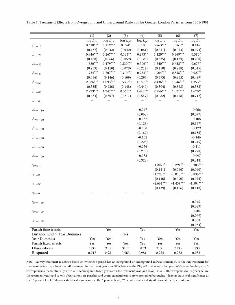
Table 1: Treatment E�ects from Overground and Underground Railways for Greater London Parishes from 1801-1901

(1) (2) (3) (4) (5) (6) (7)

logLpt logLpt logLpt logLpt logLpt logLpt logLptβτ=10 0.610*** 0.112*** 0.074* 0.100 0.763*** 0.163** 0.146

(0.137) (0.042) (0.040) (0.061) (0.251) (0.073) (0.093)

βτ=20 0.946*** 0.267*** 0.135** 0.273** 1.129*** 0.369*** 0.380*

(0.188) (0.066) (0.059) (0.123) (0.335) (0.133) (0.200)

βτ=30 1.320*** 0.479*** 0.230*** 0.506** 1.540*** 0.633*** 0.675*

(0.259) (0.110) (0.079) (0.214) (0.450) (0.228) (0.345)

βτ=40 1.734*** 0.707*** 0.319*** 0.753** 1.904*** 0.858*** 0.927**

(0.336) (0.146) (0.109) (0.297) (0.495) (0.265) (0.429)

βτ=50 2.386*** 1.093*** 0.535*** 1.166*** 2.436*** 1.246*** 1.353**

(0.535) (0.236) (0.148) (0.440) (0.594) (0.368) (0.582)

βτ=60 2.733*** 1.347*** 0.560** 1.448*** 2.756*** 1.521*** 1.670**

(0.633) (0.307) (0.217) (0.547) (0.682) (0.458) (0.717)

βτ=0 − − − − − − −

βτ=−10 -0.047 -0.066

(0.068) (0.077)

βτ=−20 -0.082 -0.108

(0.128) (0.137)

βτ=−30 -0.088 -0.129

(0.169) (0.186)

βτ=−40 -0.102 -0.146

(0.228) (0.245)

βτ=−50 -0.076 -0.111

(0.270) (0.278)

βτ=−60 -0.083 -0.097

(0.323) (0.318)

γτ=10 -1.207*** -0.291*** -0.303***

(0.141) (0.066) (0.040)

γτ=20 -1.795*** -0.813*** -0.838***

(0.146) (0.090) (0.075)

γτ=30 -2.661*** -1.459*** -1.504***

(0.139) (0.106) (0.118)

γτ=0 − − − − − − −

γτ=−10 0.046

(0.039)

γτ=−20 -0.004

(0.069)

γτ=−30 0.038

(0.084)

Parish time trends Yes Yes Yes Yes

Distance Grid × Year Dummies Yes

Year Dummies Yes Yes Yes Yes Yes Yes

Parish �xed e�ects Yes Yes Yes Yes Yes Yes Yes

Observations 3133 3133 3133 3133 3133 3133 3133

R-squared 0.917 0.981 0.963 0.981 0.924 0.982 0.982

Note: Railway treatment is de�ned based on whether a parish has an overground or underground railway station; βτ is the rail treatment for

treatment year τ ; γτ allows the rail treatment for treatment year τ to di�er between the City of London and other parts of Greater London; τ = 0

corresponds to the treatment year; τ = 10 corresponds to ten years after the treatment year (and so on); τ = −10 corresponds to ten years before

the treatment year (and so on); observations are parishes and years; standard errors are clustered on boroughs; * denotes statistical signi�cance at

the 10 percent level; ** denotes statistical signi�cance at the 5 percent level; *** denotes statistical signi�cance at the 1 percent level.

39

Figure 12: Conditional Correlation Between Bilateral Commuting Flows and Bilateral Travel Costs in 1921

-4-2

02

4R

esid

ual l

og b

ilate

ral c

omm

uter

s 19

21

-6 -4 -2 0 2 4Residual log bilateral travel cost 1921

Data Fitted

Note: Residuals from separate regressions on residence and workplace fixed effects. Sample includes all positive bilateralcommuting flows to other locations.

Figure 13: Employment by Workplace and Residence in the City of London (Model and Data) 1831-1921

1831 1841 1851 1861 1871 1881 1891 1901 1911 1921Year

0

50

100

150

200

250

300

350

400

Em

ploy

men

t (T

hous

ands

)

Data ResidentsData WorkersModel Workers

Note: “Data Residents" is employment by residence as observed in the data; “Data Workers” is employment by workplace as observed in the data;

“Model Workers” is the model’s prediction for employment by workplace; the model is calibrated to the 1921 values of rateable values, employment

by workplace and employment by residence and used to generate predictions for the removal of the railway network back to 1831.

40

Figure 14: Borough Shares of Employment by Workplace and Residence in the County of London 1831

0.0

5.1

.15

Shar

e of

Cou

nty

of L

ondo

n

BATT

ERSE

A

BERM

OND

SEY

BETH

NAL

GRE

EN

CAM

BERW

ELL

CHEL

SEA

CITY

OF

LOND

ON

DEPT

FORD

FINS

BURY

FULH

AM

GRE

ENW

ICH

HACK

NEY

HAM

MER

SMIT

H

HAM

PSTE

AD

HOLB

ORN

ISLI

NGTO

N

KENS

ING

TON

LAM

BETH

LEW

ISHA

M

PADD

ING

TON

POPL

AR

SHO

REDI

TCH

SOUT

HWAR

K

ST M

ARYL

EBO

NE

ST P

ANCR

AS

STEP

NEY

STO

KE N

EWIN

GTO

N

WAN

DSW

ORT

H

WES

TMIN

STER

WO

OLW

ICH

Employment by Workplace Employment by Residence

Figure 15: Rateable Values, Wages and Productivity in the City of London 1831-1921 (1921=1)

1831 1841 1851 1861 1871 1881 1891 1901 1911 1921Year

0

0.2

0.4

0.6

0.8

1

Val

ue R

elat

ive

to 1

921

Data Rateable ValuesModel WagesModel Productivity

Note: Rateable Values are observed in the data; the model is calibrated to the 1921 values of rateable values, employment by workplace and

employment by residence and used to generate predictions for the removal of the railway network back to 1831. Wages and productivity are

predictions from the model. Variables expressed as an index where 1921 equals one.

41

Figure 16: Rateable Values, Employment by Residence, Amenities and Residents Market Access in the City of London

1852-1921 (1921=1)

1831 1841 1851 1861 1871 1881 1891 1901 1911 1921Year

-2.5

-2

-1.5

-1

-0.5

0

0.5

1

1.5

2

2.5

log(

Val

ue /

1921

val

ue)

Data Rateable ValuesData ResidentsModel AmenitiesModel Resident Market Access

Note: Rateable Values and employment by residence are observed in the data; the model is calibrated to the 1921 values of rateable values, employ-

ment by workplace and employment by residence and used to generate predictions for the removal of the railway network back to 1831. Amenities

and resident market access are predictions from the model. Variables expressed as a log index such that 1921 equals zero.

42

Web Appendix for “The Making of the Modern Metropolis:Evidence from London (Not for Publication)

Stephan Heblich

University of Bristol

Stephen J. Redding

Princeton University, NBER and CEPR

Daniel M. Sturm

London School of Economics and CEPR

A Proof of Proposition 1

Proof. With exogenous and strictly positive location characteristics (An ∈ (0,∞), Bn ∈ (0,∞), κni ∈ (0,∞) ×

(0,∞), Ln ∈ (0,∞)), all locations are incompletely specialized as both workplaces and residences, because the

support of the Fréchet distribution for idiosyncratic amenities is unbounded from above. Using the probability of

residing in a location (equation (10) for πRn ), the probability of working in a location (equation (10) for πMn ), the zero-

pro�t condition (15), and the indi�erence condition between the city and the larger economy (11), the fraction of

workers residing in location n can be written as:

πRn =HRn

H=( γU

)ε∑s∈R

BnAε/βs κ−εnsQ

−ε(1−β)/βs Q−ε(1−α)n ,

while the fraction of workers employed in location n can be written as:

πMn =HMn

H=( γU

)ε ∑rinR

BrAε/βn κ−εri Q

−ε(1−β)/βi Q−ε(1−α)r ,

and expected worker income conditional on residing in block i from equation (20) can be written as:

vn =∑i∈R

Aε/βi κ−εniQ

−ε(1−β)/βi∑

s∈RAε/βs κ−εnsQ

−ε(1−β)/βs

[A

1/βi Q

−(1−β)/βi

],

and the land market clearing condition from equation (18) can be written as:(1− ββ

)wnπ

Mn

Qn+ (1− α)

vnπRn

Qn=LnHn

.

Combining the above relationships, this land market clearing condition can be re-expressed as:

Dn(Q) = 1−ββ

[A1/βn

Q1+(1−β)/βn

] [∑r∈R

BrAε/βi κ−εri

Qε(1−β)/βi Q

ε(1−α)r

]+ 1−α

Qn

[∑i∈R

(Aε/βi κ−εni Q

−ε(1−β)/βi∑

s∈R Aε/βs κ−εnsQ

−ε(1−β)/βs

)A

1/βi

Q(1−β)/βi

] [∑s∈R

BnAε/βs κ−εns

Qε(1−β)/βs Q

ε(1−α)n

]− Ln = 0,

for all n ∈ R, where we have chosen units in which to measure utility such that (U/γ)ε/H = 1. The above land

market clearing condition provides a system of equations for theN boroughs in terms of theN unknown �oor prices

Qn, which has the following properties:

limQn→0

Dn(Q) =∞ > Ln, limQn→∞

Dn(Q) = 0 < Ln,

1

dDn(Q)

dQn< 0,

dDn(Q)

dQi< 0,

∣∣∣∣dDn(Q)

dQn

∣∣∣∣ > ∣∣∣∣dDn(Q)

dQi

∣∣∣∣ .It follows that there exists a unique vector of residential �oor pricesQ that solves this system of land market clearing

conditions. Having solved for the vectors of �oor prices (Q), the vector of wages w follows immediately from the

zero-pro�t condition for production (15). Given �oor prices (Q) and wages (w), the probability of residing in a location

(πR) follows immediately from (10), and the probability of working in a location (πM

) follows immediately from (10).

Having solved for {πM, πR

,Q,w}, the total measure of workers residing in the city can be recovered from our choice

of units in which to measure utility (U/γ)ε/H = 1), which together with population mobility (11) implies:

H =

[∑r∈R

∑s∈R

Brwεs

(κrsQ

1−αr

)−ε].

We therefore obtain HM = πMH and HR = πRH . This completes the determination of the equilibrium vector

{πM, πR

, H ,Q, w}.

2