Th

e M

ak

ing

of G

lob

al F

ina

nc

e 1

880-1

913

OECD's books, periodicals and statistical databases are now available via www.SourceOECD.org, our online library. This book is available to subscribers to the following SourceOECD themes:DevelopmentFinance and Investment/Insurance and PensionsGeneral Economics and Future StudiesAsk your librarian for more details of how to access OECD books on line, or write to us atSourceOECD@oecd.org

This book traces the roots of global financial integration in the first “modern” eraof globalisation from 1880 to 1913. It analyses the direction, destinations andorigins, of international financial flows in order to determine the domestic policychoices that either attracted or deterred such flows to developing countries.

The book deposes the idea that the gold standard and other institutionalarrangements were the key to attracting foreign investment, pointing to thestability and probity of political systems as much more important. One of the majorconclusions is that the successful management of international financialintegration depends primarily on broad institutional and political factors, as well ason financial policies, rather than simply opening or closing individual economies tothe international winds.

The Making of Global Finance 1880-1913 can serve as a valuable tool to current-day policy dilemmas by using historical data to see which policies in the past ledto enhanced international financing for development. It also includes historicaldata that will interest all scholars of economics and economic history, as well asthe casual reader.

Development Centre Studies

The Making of Global Finance 1880-1913

ISBN 92-64-01534-541 2004 03 1 P-:HSTCQE=UVZXYU:

www.oecd.org

«Development Centre Studies

The Making of Global Finance1880-1913

By Marc Flandreau and Frédéric Zumer

This work is published under the auspices of the OECDDevelopment Centre. The Centre promotes comparative development analysis and policy dialogue, as described at:

www.oecd.org/dev

DEVELOPMENT CENTRE OF THE ORGANISATION FOR ECONOMIC CO-OPERATION AND DEVELOPMENT

DEVELOPMENT CENTRE STUDIES

The Making of Global Finance 1880-1913

By Marc Flandreau and Fédéric Zumer

ORGANISATION FOR ECONOMIC CO-OPERATIONAND DEVELOPMENT

Pursuant to Article 1 of the Convention signed in Paris on 14th December 1960,and which came into force on 30th September 1961, the Organisation for EconomicCo-operation and Development (OECD) shall promote policies designed:

– to achieve the highest sustainable economic growth and employment and a risingstandard of living in member countries, while maintaining financial stability, andthus to contribute to the development of the world economy;

– to contribute to sound economic expansion in member as well as non-membercountries in the process of economic development; and

– to contribute to the expansion of world trade on a multilateral, non-discriminatorybasis in accordance with international obligations.

The original member countries of the OECD are Austria, Belgium, Canada, Denmark,France, Germany, Greece, Iceland, Ireland, Italy, Luxembourg, the Netherlands, Norway,Portugal, Spain, Sweden, Switzerland, Turkey, the United Kingdom and the United States.The following countries became members subsequently through accession at the datesindicated hereafter: Japan (28th April 1964), Finland (28th January 1969), Australia(7th June 1971), New Zealand (29th May 1973), Mexico (18th May 1994), the Czech Republic(21st December 1995), Hungary (7th May 1996), Poland (22nd November 1996), Korea(12th December 1996) and the Slovak Republic (14th December 2000). The Commission of theEuropean Communities takes part in the work of the OECD (Article 13 of theOECD Convention).

The Development Centre of the Organisation for Economic Co-operation and Development wasestablished by decision of the OECD Council on 23rd October 1962 and comprises twenty-two membercountries of the OECD: Austria, Belgium, Canada, the Czech Republic, Denmark, Finland, France,Germany, Greece, Iceland, Ireland, Italy, Korea, Luxembourg, Mexico, the Netherlands, Norway, Portugal,Slovak Republic, Spain, Sweden, Switzerland, as well as Chile since November 1998 and India sinceFebruary 2001. The Commission of the European Communities also takes part in the Centre’sGoverning Board.

The purpose of the Centre is to bring together the knowledge and experience available inmember countries of both economic development and the formulation and execution of generaleconomic policies; to adapt such knowledge and experience to the actual needs of countries or regionsin the process of development and to put the results at the disposal of the countries by appropriatemeans.

The Centre is part of the “Development Cluster” at the OECD and enjoys scientific independencein the execution of its task. As part of the Cluster, together with the Centre for Co-operation withNon-Members, the Development Co-operation Directorate, and the Sahel and West Africa Club, theDevelopment Centre can draw upon the experience and knowledge available in the OECD in thedevelopment field.

THE OPINIONS EXPRESSED AND ARGUMENTS EMPLOYED IN THIS PUBLICATION ARE THE SOLERESPONSIBILITY OF THE AUTHORS AND DO NOT NECESSARILY REFLECT THOSE OF THE OECDOR THE GOVERNMENTS OF THEIR MEMBER COUNTRIES.

** *

Publié en français sous le titre :

Les origines de la mondialisation financière 1880-1913

© OECD 2004

Permission to reproduce a portion of this work for non-commercial purposes or classroom use should be obtained through theCentre français d’exploitation du droit de copie (CFC), 20, rue des Grands-Augustins, 75006 Paris, France, tel. (33-1) 44 07 47 70,fax (33-1) 46 34 67 19, for every country except the United States. In the United States permission should be obtainedthrough the Copyright Clearance Center, Customer Service, (508)750-8400, 222 Rosewood Drive, Danvers, MA 01923 USA,or CCC Online: www.copyright.com. All other applications for permission to reproduce or translate all or part of this bookshould be made to OECD Publications, 2, rue André-Pascal, 75775 Paris Cedex 16, France.

3

Foreword

The 2001-2002 OECD Development Centre Work Programme, Globalisationand Governance, revealed a number of transversal issues relevant to virtually all thethemes. This book is the result of steps to cover some of those issues.

4

Acknowledgements by the Authors*

The research summarised in this monograph was initiated several years ago, in1995. A variety of institutions and colleagues have supported it materially andintellectually throughout. We benefited from financial support from the ObservatoireFrançais des Conjonctures Économiques (O.F.C.E.) in Paris, as well as from a varietyof grants from the French Ministry of Research. It is a pleasure to acknowledge thisdebt. We also received much feedback from numerous colleagues who supported usthrough their comments, criticism and encouragement, and in many other ways too.For their friendly advice and continued discussion we especially wish to thank AmiyaKumar Bagchi, Michael Bordo, Steve Broadberry, Forrest Capie, Filippo Ceserano,Daniel Cohen, Jerry Cohen, Marcello de Cecco, Barry Eichengreen, Luca Einaudi,Niall Ferguson, Curzio Giannini, Maria Alejandra Irigoin, Patrick O’Brien, LeandroPrados della Escosura, Jaime Reis, Albrecht Ritschl, Emma Rothschild, Anna Schwartzand Giuseppe Tattara.

The database presented here involved a massive effort. For their help withsupplying directions to appropriate sources we thank Michael Bergman, Felix Butschek,Olga Christodoulaki, Jean-Pierre Dormois, Paul Gregory, Ingrid Henriksen, LarsJonung, Anton Kausel, John Komlos, Pablo Martin Acena, Andreas Resch, Max-StefanSchulze, Jan-Pieter Smits, Giuseppe Tattara, Bruno Théret, Jan-Luiten Van Zanden,André Villella and Vera Zamagni. Special gratitude is due to Roger Nougaret, head ofthe Archives at Crédit Lyonnais, for pointing out to us that the Lyonnais’ country-assessment files were possibly outstanding sources to reconstruct macroeconomicindicators. When this turned out to be the case indeed, Roger kindly and patientlymade all the material we needed available for extensive periods, thus tremendouslyfacilitating our efforts. As we stretched his patience and that of his team he kepthelping out in the kindest way.

The help of several students is gratefully acknowledged. We especially thankJérôme Legrain for his work on the Statesman’s Year Book and Ignacio Briones forcomputing the exchange-rate volatility indices. Juan Flores contributed by helpingout with the Latin American countries. An expanded database for Latin America willshortly become available as part of his ongoing dissertation.

5

The present monograph was presented in a variety of places, including mostprominently the OECD Development Centre seminar (Paris, April 2002) which provedessential in bringing the project to fruition. In addition, we are grateful to participantsto the Universidad Carlos III economic history seminar (Madrid, May 2002), theHumboldt Universität Departmental seminar (Berlin, May 2002), the Venice InternationalUniversity Summer School (Venice, September 2002), the Cambridge University“Economics and History” Lectures (Cambridge, February 2003), the Banca d’Italiaeconomic history seminar (Rome, March 2003) and the OFCE Convergences inEconomic History Seminar in Paris (April 2003). The suggestions and reactions ofthe audiences proved most useful in fostering our thinking.

Finally, for their detailed remarks on earlier drafts we especially wish to thankJorge Braga de Macedo and Colm Foy at the OECD Development Centre in Paris.

This book is dedicated to the memory of Charles P. Kindleberger for hiscomments, criticism and, above all, inspiration.

________________________

The OECD Development Centre would like to thank the Government of Portugalfor its generous financial contribution to the successful completion of this project.

______________________________* Marc Flandreau is professor of economics at the Institut d’Études Politiques de Paris

and research associate at OFCE. He is also a research fellow of the Centre for EconomicPolicy Research in London and a senior adviser for Lehman Bros., France. He haspublished extensively on international finance and monetary history. His articlesappeared in the European Economic Review, the Journal of International Economics,the Journal of Money, Credit and Banking, Economic Policy, and the Journal ofEconomic History. He is the author of The Gold Standard in History and Theory (withBarry Eichengreen), Routledge, 1997; The Glitter of Gold. France, Bimetallism and theEmergence of the International Gold Standard 1848-1873, Oxford, 2003; MoneyDoctors: the Experience of International Financial Advising 1850-2000,Routledge, 2003; and International Financial History in the XXth Century: System andAnarchy (with Harold James and Carl-Ludwig Holtfrerich), Cambridge, 2003.

Frédéric Zumer is professor of economics at the University Pierre Mendès France,Grenoble, and research associate at OFCE. His work on European macroeconomic stabilityhas appeared in many journals including the Journal of Public Economics, the CarnegieRochester Conference Series, and Economic Policy. He is a leading authority on cycles,redistribution and stabilisation in Europe.

7

Table of Contents

Acknowledgements by the Authors ............................................................................... 4

Preface Jorge Braga de Macedo ................................................................................ 9

Introduction: Reputation and Development ................................................................... 11

I. The Rules of the Game: Interest Convergence and Financial Globalisation ........ 17

II. Worshipping Mammon ............................................................................................ 21

III. Religion and other Dummies ................................................................................... 24

IV. Micro Motives and Macro Behaviour .................................................................... 27

V. What’s on Man’s Mind: Theories in Use ............................................................... 30

VI. Empirical Evidence: Interest Spreads and the Debt Burden .................................. 36

VII. Thresholds of Confidence ....................................................................................... 40

VIII. Convergence Explained ........................................................................................... 45

IX. Developmental Consequences ................................................................................ 48

X. Policy Lessons and Conclusions ............................................................................ 55

Technical Appendix .......................................................................................................... 71

Statistical Appendix: The Making of Global Finance: A Database ............................... 95

Database Tables ............................................................................................................... 109

Bibliography ..................................................................................................................... 135

9

Preface

The OECD Development Centre’s 2001-2002 Programme of Work on“Globalisation and Governance” (G&G) showed that well governed developing countriestend to benefit from globalisation. Positive G&G interaction requires policy credibilityon national, regional and global levels. If financial crisis in some countries leads tosudden stops in capital flows to others, globalisation can reverse development: theG&G interaction may be negative.

The debate on monetary integration and exchange rate regimes, whose roots goback to the first age of globalisation, reflects this complex interaction. At a 2001Development Centre Seminar, Marc Flandreau presented his original series of fiscaland monetary variables for sovereign borrowers and showed the determining influenceof financial and political reputation for bond market spreads. Based on some of thatdiscussion, this book confirms that in the past a positive G&G interaction was alreadyessential in investors’ perceptions of development prospects in what were then calledcapital-poor countries.

The concern with governance dominates cultural stereotyping of “Latin” versus“Nordic” sovereign borrowers and contrasts with the alleged preference of investorsgenerally for authoritarian regimes. To the extent that a disenfranchised populationpays lower taxes, narrowing and lowering state revenues with a heightened risk ofinstability, a combination of political and financial freedom is most attractive to investorsin capital-poor countries.

The authors use their data set to analyse financial flows in a period of intensivecapital movement, and find that it was the quality of the fundamentals that droveinvestors’ choices, rather than adherence, or not, to the gold standard. Expert opinionof the time set indicators of sound fundamentals as a ratio of debt service to exportsbelow 20 per cent and a ratio of debt service to government revenues below 35 percent, which the authors here label the “trade” and the “tax” tests. They show that thetax test (which reflects a greater concern with governance, including politicalparticipation) gradually replaced the trade test, which only reflects openness. Usually,the tax test is more pessimistic than the actual spread.

10

The movement towards concern with political governance followed the 1890Baring crisis — and is an element in explaining why the risk of default declines withthe extension of the franchise. For example, with the 1910 Republican revolution incapital-poor Portugal, the franchise was extended to cover 6.2 per cent of thepopulation, from only 2.5 per cent previously. The effect was a decline of over 20 percent in the probability of default in 1911, more than twice the sample average.

This book confirms that adopting a common monetary standard does not providea fast road to policy credibility. Much more important are governance structures andinstitutions which imply predictability and stability, especially when the economy isgrowing rapidly as many did during the first age of globalisation. Then as now, apositive G&G interaction is the only basis for investor confidence and improvedprospects for capital-poor countries to attract finance for development. It also reflectsand sustains worldwide economic Growth, bringing in a third, and crucial, G.

Jorge Braga de MacedoPresident, OECD Development Centre,

Paris, 30 June 2003

11

The Making of Global Finance 1880-1913

Introduction: Reputation and Development

Unless we know why people expect what they do expect, any explanationthat refers to expectations as causa efficientes is worthless.

Joseph Aloys Schumpeter, Business Cycles, 1939

What guides investors’ decisions? How is market sentiment shaped, and howdoes this influence the course of global financial integration? Economics hasstraightforward answers. Modern theories help identify the relevant variables thatresearchers ought to consider when trying to explain both individual choices andaggregate outcomes at any moment. The theories are then tested on the variables thusdefined. This method is valid in any sample period, and the same models should beable to account for both present and past phenomena. Economics provides the analyticaltools through which we can interpret numbers.

This approach, which sometimes gives short shrift to that of historians, hasscientific virtues but also inherent limitations. It has generated or at least justified aseemingly natural division of labour between economic analysis and data gathering.Statisticians and economic historians may collect the relevant numbers, whicheconomists use later to implement models developed deductively. The numbers mayserve as little more than fodder for intellectually powerful, but not necessarily correcttheories. Other disciplines, such as physics, where the methodology is inductive (apartfrom the sub-branch of theoretical physics) generally recognise that the separation ofobservation and analysis is meaningless.

Perhaps no other context more aptly illustrates this simple but far-reaching pointthan that of the perceptions by market participants of the quality of government policies.It is well known that consensus develops regarding the appropriate policies countriesshould adopt given the times and circumstances. The “Washington consensus” of the1990s, which favoured openness and liberalisation, was an illustration. Consensusdoes matter because it helps define “best practices” in policy making. Policy makersget judged on their ability at implementing the policies considered as a test of policy

12

success. In an affluent international financial system where countries compete toattract capital, market participants reward policy makers through lower borrowingcosts and a greater supply of funds1. If this is true, certain variables should play a kindof focal role for investors who monitor policy developments. Concerns about themshould lie at the heart of policy making, because the authorities will have to worryabout getting the variables right. Economists and political scientists describe suchsituations as policy regimes2.

It is fairly difficult, however, to document these highly important policy issuesfrom a purely abstract model. Pinning down the relevant variables and their influenceon market perceptions (let alone how policies themselves react to them) is by nomeans easy. Pure theory is a poor guide. Beliefs shape policy practices and policypractices shape beliefs. It is an established result in economic theory that forward-looking expectations lead to multiple equilibriums. This means that examining a givensituation or equilibrium says nothing about the forces that have brought it about. Theonly way to sort out these difficulties is to open the black box of market perceptionsto see how they determine the allocation of capital.

To make this point, this monograph considers the first large experiment in financialglobalisation. It occurred in the second half of the 19th century when capital flowswere basically unrestrained, with a potentially very high degree of capital mobility.Empirical evidence provided by the Feldstein-Horioka measures of financial integrationsupport the consensus view that during those years financial integration was indeedvery great. It shows conclusively that the late 19th century displayed a very highdegree of current-account openness, illustrated by a large disconnection betweendomestic saving and investment3. This integration has only recently been revived,thus raising the possibility of many useful parallels between the first age of globalisation(1848-1914) and the second (1973 to the present)4.

Nevertheless, understanding the sources of international financial integrationbefore World War I has remained a major challenge. Following a view that emergedin the inter-war period when contemporaries associated the dislocations of the globaleconomic system with those of the global exchange-rate system, scholars often pointto the gold standard as the backbone of pre-1914 integration. The international goldstandard was an informal arrangement whereby countries independently fixed andsought to defend the value of their currencies in terms of gold or some gold-relatedunit, thus creating a de facto fixed exchange-rate system among followers of thispolicy rule. As a regime, it thus provided both a stable exchange-rate environment anda number of policy prescriptions, because monetary expansion beyond a certain pointwas over the long run incompatible with maintenance of the gold parity.

Analysts have therefore come to see the pre-1914 gold standard as the epitomeof what a global policy consensus could be. The supposedly restrictive policies of theso-called “classical” gold standard have been often described as an ethos developedduring the long boom of the late 19th and early 20th centuries, and that acted as adisciplining device promoting financial sobriety. As a result, “the gold standard came tosymbolise the mentality and patterns of conduct of the intellectual and economic elite”.

13

Policy makers expected that the market would expect them to remain on gold andadjusted their behaviour correspondingly. As a regime, the gold standard is said to haveembedded the list of orthodox recipes that became the backbone of the policy consensusof the time5.

Some argue that this mentality played a decisive role in shaping later responsesto economic turmoil. Policy makers were prepared to go to any lengths to avoiddevaluation. When crisis hit in the inter-war years, governments and leaders trainedduring the pre-war period reached for gold adherence as a natural remedy. This canexplain the troubling persistence of deflationary policies during most of the GreatDepression and why governments resisted the lax policies that any modernundergraduate student would recommend. Gold became the millstone around the neckof national economies, helping them to sink (Eichengreen and Temin, 2000).

The reference to “mentality” is undoubtedly a radical way to solve the conundrumof expectations and policies. In any case, one should definitely ponder the broaderimplications of this strategy, which raises questions that obviously go beyond thespecific issues of the inter-war crisis. All too often, “mentality” is treated as somekind of residual that remains when other factors have been taken into account. Yetwhen it determines the very credibility of policy actions, it arguably becomes theprincipal factor. It would be very helpful to have a method to identify the variablesthat mattered most in shaping contemporaries’ beliefs. Under the gold standard, didpeople worry about the exchange-rate regime (adherence to gold), fiscal policy(balanced budgets) or monetary policy (a sound currency)? What weights did marketparticipants and policy makers give to these alternative goals? If 19th century orthodoxwriters had been asked to choose between, say, adherence to gold and fiscal balance,what would have they preferred?

Proper answers to these questions are essential given the difficulties in makingcomparisons between the first and the second eras of globalisation. To a very largeextent, globalisation takes place today in a system of essentially floating exchangerates (at least among developed areas such as Europe, Japan and the United States)without this constituting a major obstacle6. If the conventional view on the sources ofpre-1914 globalisation is correct, if it rested on a sustained belief in the virtues offixed exchange-rate regimes, one would have to admit that a major paradigm shift hasoccurred and that the modern drivers of globalisation are radically different. Today(after, it is true, several decades of debate) the choice of the exchange-rate regime hasbecome a less and less distinctive item on the good-governance menu7.

This monograph studies the roots of credibility during the first era of globalisation.It gives much attention to economic ideas regarding best policy practices. It focuseson the views of those involved in international macroeconomics (as the subject isknown today) during the years when the gold standard ethos supposedly coagulated.It tries to develop a method that facilitates study of investors’ thinking and behaviour“in the wild”, as anthropologists say. The acid test of the intuitions formalised herewill be the ability of the methodology to make sense of the well-known but so far

14

unexplained phenomenon of interest-rate convergence over 1875-1913, which resultedin very low interest premiums paid by most countries during the early 1900s. Thebroad goal is more ambitious — to explain the making of global finance.

The study develops a new, “grass-roots” analysis. It follows an inductiveapproach, and, rather than projecting modern theories — some would say modernprejudices — onto past data, it considers the theories in use at the time under study.Archival and secondary sources are used to reconstruct what people in both academiaand financial circles thought good macroeconomic policy management should be.This allows the formulation of assumptions about what types of variables peopleought to have considered, and in turn naturally leads to an empirical discussion of thevalidity of the behavioural model thus constructed. This approach avoids the pitfallsof a posteriori reconstruction. It provides a way to determine what macroeconomicindicators truly mattered, and it can challenge the myth of the gold standard ideology.

To test whether contemporary theories influenced pricing behaviour requiresobtaining the information set available to contemporary investors. A vast databasewas therefore gathered, for a sample of 17 countries over 34 years (1880-1913). Thewide array of nations8 includes both capital-rich and capital-poor countries, in bothEurope and Latin America, both South and North9. This database differs from existingones in being larger (especially for capital-poor countries, for which figures are harderto get) and in including more variables. Unlike those in other studies, this database,because it makes extensive use of archival sources, is as close as possible to theinformation monitored by contemporary investors. Collecting it also helped to revealflaws in the official sources normally used in similar studies. Contemporary observersoften knew of them and routinely adjusted official figures when they included knownbiases. Investors, the study finds, knew better than modern scholars working withofficial retrospectives.

Combining the analysis of beliefs and the data thus collected, the study thenproceeds to reconstruct from the theories in use a more meaningful and relevant pictureof investors’ behaviour under the gold standard. Given the importance that writershave given to the Belle Epoque record to account for inter-war problems, and givenits parallels with today’s globalisation, this exercise provides a wealth of theoretical,historical and, above all, policy lessons. It provides an opportunity to revisit a numberof important debates on the relations between development and international financialintegration. It shows that technology (financial innovation) did not play a leading rolein promoting the globalisation of capital. Simple policies that mechanically favouropenness (such as free trade) were not essential either. Instead, the making of globalfinance rests on striking a careful balance between fiscal development and economicgrowth. The ability of states to collect resources and maintain strong records of interestpayments determines the cost at which they can attract capital. This brings to the forethe question of governance as a key feature of financial globalisation and thus puts thestate back into the supposedly laissez-faire pre-1914 context, a conclusion anticipatedby Alexander Gerschenkron (1962) in a different perspective.

15

Section I sets the analytical stage by relating capital markets integration and thecost of capital imports. It also identifies interest-rate convergence as a key aspect ofthe integration of the pre-1914 international financial system. Section II reviews existingattempts to explain interest-rate convergence. Section III outlines the weaknesses of“regime” dummies in empirical studies. Section IV provides an outline of themethodology, showing that contemporary ratings of sovereign risk display a highcorrelation with market prices. This demonstrates that it is useful to documentperceptions from a survey of contemporary sources. Section V surveys the theoriesand views regarding sound macroeconomic management used by contemporaries ofthe pre-WWI international financial system to assess sovereign risks. Sections VIand VII exploit the results of this survey to develop and test, using the new database,two alternative models explaining the pricing of sovereign bonds. The results point toa ranking of the macroeconomic priorities in the minds of 19th century investors thatcontradicts the main claims of the conventional literature on the pre-war gold standard.Section VIII solves the convergence puzzle. It outlines the importance of successfuldevelopment strategies in bringing about interest-rate convergence. Section IX developsthis point by relating alternative rating techniques to alternative development views.Section X provides conclusions and policy lessons.

17

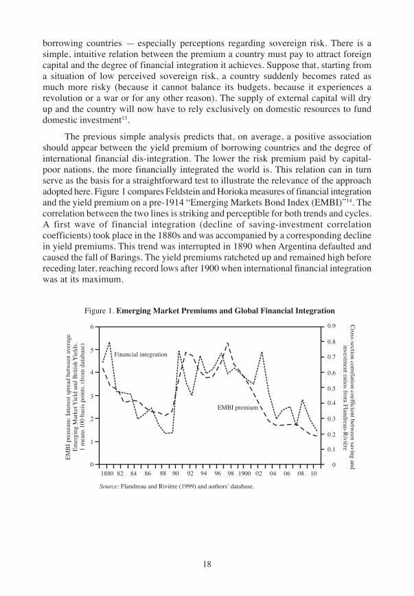
I. The Rules of the Game: Interest Convergenceand Financial Globalisation

To clarify the discussion, it is useful to start from a simple analysis of therelation between perceptions of sovereign risk and measures of financial integration10.One feature of the first era of globalisation, common to the second as well, was analmost complete absence of formal barriers to the free mobility of capital. Apart fromsmall taxes on foreign-exchange transactions (motivated by financial considerations)and a measure of control on initial public offerings (politically motivated), portfolioreallocation, international bond circulation, etc. were basically left unhampered11. Anabundant literature has shown that, indeed, the prices of similar bonds quoted inseveral markets were fully arbitraged12.

Was this structural situation of basically free capital mobility conducive to ahigh level of financial integration, i.e. was the actual movement of capital effectivelyas large as it might have been? The possibility for capital to migrate suffices to equalisethe prices of identical assets in various markets, but that does not mean that largeflows of capital take place. The analytical workhorse to address whether capital didmove consists of the Feldstein and Horioka (1980) measures of financial integration.Intuitively, their rationale is that a low correlation between domestic saving andinvestment reveals that investment is not constrained by domestic resources. This istantamount to saying that the degree of financial integration is high. Therefore, to trackthe ebbs and flows of global finance, these measures compute cross-section correlationcoefficients between saving and investment ratios, for a given sample of countries andfor a given year: the lower the correlation, the higher the integration. The resultingtime series of correlation coefficients captures the evolution of financial integration.

Many authors (e.g. Obstfeld and Taylor, 1998) have pointed out the apparentsimilarity between coefficients computed for recent periods and for a century ago(with a period of deglobalisation coinciding with the Great Depression). Yet few havenoted that international financial integration fluctuated quite widely even within periodswith high average financial integration, such as before 1914. Consensus estimates, forinstance, show progress in international financial integration in the 1880s, followedby a brutal interruption in the early 1890s, resumption after 1895 and progressafterwards that surpassed the levels of the late 1880s.

A priori, several factors might have accounted for that. Technologicalimprovements can be brushed aside as secondary at best; had they truly mattered, theprogress of financial integration should have been much more regular, and reversalsshould not have occurred. The factors favoured here, which this monograph documentsin detail, embrace market perceptions regarding the quality or “soundness” of

18

borrowing countries — especially perceptions regarding sovereign risk. There is asimple, intuitive relation between the premium a country must pay to attract foreigncapital and the degree of financial integration it achieves. Suppose that, starting froma situation of low perceived sovereign risk, a country suddenly becomes rated asmuch more risky (because it cannot balance its budgets, because it experiences arevolution or a war or for any other reason). The supply of external capital will dryup and the country will now have to rely exclusively on domestic resources to funddomestic investment13.

The previous simple analysis predicts that, on average, a positive associationshould appear between the yield premium of borrowing countries and the degree ofinternational financial dis-integration. The lower the risk premium paid by capital-poor nations, the more financially integrated the world is. This relation can in turnserve as the basis for a straightforward test to illustrate the relevance of the approachadopted here. Figure 1 compares Feldstein and Horioka measures of financial integrationand the yield premium on a pre-1914 “Emerging Markets Bond Index (EMBI)”14. Thecorrelation between the two lines is striking and perceptible for both trends and cycles.A first wave of financial integration (decline of saving-investment correlationcoefficients) took place in the 1880s and was accompanied by a corresponding declinein yield premiums. This trend was interrupted in 1890 when Argentina defaulted andcaused the fall of Barings. The yield premiums ratcheted up and remained high beforereceding later, reaching record lows after 1900 when international financial integrationwas at its maximum.

Financial integration

EMBI premium

6

5

4

3

2

1

0

0.9

0.8

0.7

0.6

0.5

0.4

0.3

0.2

0.1

01880 82 84 88 90 92 94 96 98 1900 02 04 06 08 1086

Figure 1. Emerging Market Premiums and Global Financial Integration

Source: Flandreau and Rivière (1999) and authors’ database.

EMBI

pre

miu

m: I

nter

est s

prea

d be

twee

n av

erag

eEm

ergi

ng M

arke

tYie

ld a

nd B

ritish

Yiel

ds.

1 m

eans

100

bas

is po

ints.

(fro

m d

atab

ase)

Cross-section correlation coefficient between saving and

investment ratios from

Flandreau-Rivière

19

Several implications appear. First, the process of financial globalisation beforeWWI was not linear. It fluctuated a lot. In a general context of free internationalcapital mobility or, differently put, in the absence of formal capital controls, theactual degree of international financial integration and thus the extent to which theinternational system avails itself of the benefits of globalisation may vary considerably15.These variations seem tightly related to the perceived risks of lending to emergingeconomies, because the interest premiums borrowing countries face measure theperceived default risks. Borrowing costs and financial integration may be seen as thetwo sides of the same coin; they obey the same laws of motion.

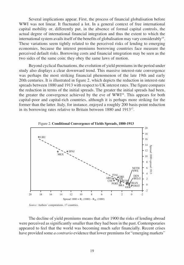
Beyond cyclical fluctuations, the evolution of yield premiums in the period understudy also displays a clear downward trend. This massive interest-rate convergencewas perhaps the most striking financial phenomenon of the late 19th and early20th centuries. It is illustrated in figure 2, which depicts the reduction in interest-ratespreads between 1880 and 1913 with respect to UK interest rates. The figure comparesthe reduction in terms of the initial spreads. The greater the initial spreads had been,the greater the convergence achieved by the eve of WWI16. This appears for bothcapital-poor and capital-rich countries, although it is perhaps more striking for theformer than the latter. Italy, for instance, enjoyed a roughly 200 basis-point reductionin its borrowing rates relative to Britain between 1880 and 191317.

URU

MEXSPAI

ITALARG

CHIGRE

PORTRUSS

BRAFRAN

SWITGER

Spread 1880 = R (1880) - R (1880)

Source: Authors’ computations, 17 countries.

20 18 16 14 12 10 8 6 4 2 0 -2

20

18

16

14

12

10

8

6

4

2

0

-2

Figure 2. Conditional Convergence of Yields Spreads, 1880-1913

AH BELGDEN

SWENETH

Spread 1880-spread 1913

i uk

The decline of yield premiums means that after 1900 the risks of lending abroadwere perceived as significantly smaller than they had been in the past. Contemporariesappeared to feel that the world was becoming much safer financially. Recent criseshave provided some a contrario evidence that lower premiums for “emerging markets”

20

mean smoother financing of their current accounts by the capital market, and thesame should basically apply to any other country. It is thus tempting to relate the well-known financial stability of the early 20th century to the lower risk premiums countriesfaced throughout the world.

This suggests a straightforward interpretation of financial globalisation beforeWorld War I. The progress of integration after 1900 might be seen as a gradualrightwards shift of the supply curve of capital arising from successive reductions inlending premiums, which in turn supported ever-rising capital movements. A largeliterature has shown that the export of capital peaked in those years — British capitalexports, for instance, reached 10 per cent of national income. In this view, after themid-1890s, the global capital market became friendly to borrowing countries, whichbegan to exploit to their full extent the benefits of free capital mobility18.

The careful analyst, however, may point out that the correlation exhibited inFigure 1 could work the other way around. Suppose that “animal spirits” led for nosound reasons to an increase in capital exports. This is likely if, as suggested byKindleberger (1988), “manias” drive both domestic and international financialmarkets19. Regardless of the actual risks, the supply curve of capital still shifts to theright, causing yield premiums to decline. The association depicted in Figure 1 remains,but the causality is reversed. In this case, financial integration proceeds randomly as aresult of mood changes and drives the fluctuations in yield prices. Thus the questionarises: What drove the process of financial integration? Identifying empirically thevariables that affected risk premiums can put one in a better position to sort out thecausality and provide an interpretation of the sources of pre-1914 globalisation.

21

II. Worshipping Mammon

The usual suspect for explaining pre-1914 financial globalisation is the goldstandard. This system, initially adopted only by Britain (1821), Portugal (1854) anda few German towns, gradually expanded over the second half of the 19th century. Afirst wave took place during the 1870s, after France unofficially put an end tobimetallism (Flandreau, 1996, 2003a). The process stalled in the early 1890s, and apartial reversal occurred when some countries that had operated or shadowed a goldstandard experienced exchange crises. Propagation resumed in the late 1890s andearly 1900s, with the final outcome being a fairly brief period, 1900-13, when most ofWestern Europe, the Americas and portions of Asia were on gold. A landmark ofglobal exchange-rate stability, this episode became known as the heyday of the goldstandard20. Most later observers were quick to relate the simultaneous record highs offinancial globalisation with the gold standard’s reaching its maximum geographic scope.A regime had spread, borrowing premiums had declined and capital markets hadglobalised. It ended in a bloodbath, but a powerful myth had been born.

The resulting nostalgia cast a long shadow on 20th century monetary thinking,a shadow extending until the most recent developments of macroeconomic history.The conventional view holds that “[I]t is of course common knowledge that Britishinvestors viewed securities issued by countries not on the gold standard as riskier thanthose of countries that were.” (Madden, 1985, p. 255.) Countries on gold did paylower interest rates, and the decline in interest differentials was seen as resulting fromthe spread of the gold standard21. Academic product differentiation has led to marginallydifferent formulations of the underlying economic mechanism, but the basic point iseverywhere the same. Some prefer to emphasise the incentives associated with goldadherence; being on gold signalled a commitment to “good” macroeconomic policies— the popular “good housekeeping seal of approval” story22. Others stress that goldadherence provided greater capital market integration through exchange-rate stability;the gold standard reduced transaction costs and uncertainty (Obstfeld andTaylor, 2003a, 2003b). They have portrayed the spread of the gold standard assupporting a transition from “autarky” in the 1870s to “integration” after 1900 (Clemensand Williamson, 2002). Whether through improved reputations, reduced uncertaintyor both, all these interpretations assume gold adherence to have shifted the supplycurve of foreign capital to the right and thus associated it with the decline of interest-rate premiums and financial integration.

The empirical workhorses of this literature are gold standard “dummies” used tocapture the effect of gold adherence on borrowing terms23. The pioneering work ofBordo and Rockoff (1996) reported that participation in the so-called gold “club” was

22

associated with a reduction of marginal borrowing rates of about 50 basis points.Strikingly, gold adherence in this study and subsequent similar ones has always beenthe only statistically significant relevant variable24.

In view of the problems discussed in this monograph, these findings provide anatural starting point, at the heart of empirical investigation of the existence of a policyconsensus during the first era of globalisation. If floating was, before WWI, associatedwith substantially higher borrowing rates, one may understand why governments,concerned with securing the best possible terms for their own loans, inadvertentlysucceeded in building a harmonious international financial architecture by all movingto gold25. The gold standard and its rewards would have been the invisible hand thatprovided for “spontaneous” global harmony.

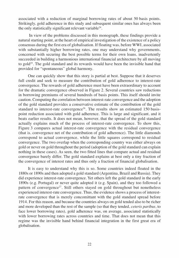
One can quickly show that this story is partial at best. Suppose that it deservesfull credit and seek to measure the contribution of gold adherence to interest-rateconvergence. The rewards of gold adherence must have been extraordinary to accountfor the dramatic convergence observed in Figure 2. Several countries saw reductionsin borrowing premiums of several hundreds of basis points. This itself should invitecaution. Computing the correlation between interest-rate convergence and the adoptionof the gold standard provides a conservative estimate of the contribution of the goldstandard to interest-rate convergence26. The results show an estimated 150 basis-point reduction associated with gold adherence. This is large and significant, and itbeats earlier results. It does not mean, however, that the spread of the gold standardactually explains much of the process of interest-rate convergence. To show this,Figure 3 compares actual interest-rate convergence with the residual convergence(that is, convergence net of the contribution of gold adherence). The little diamondscorrespond to actual convergence, while the little squares correspond to residualconvergence. The two overlap when the corresponding country was either always ongold or never on gold throughout the period (adoption of the gold standard can explainnothing in these cases). As seen, the two fitted lines that compare actual and residualconvergence barely differ. The gold standard explains at best only a tiny fraction ofthe convergence of interest rates and thus only a fraction of financial globalisation.

It is easy to understand why this is so. Some countries indeed floated in the1880s or 1890s and then adopted a gold standard (Argentina, Brazil and Russia). Theydid experience interest-rate convergence. Yet others left the gold standard in the early1890s (e.g. Portugal) or never quite adopted it (e.g. Spain), and they too followed apattern of convergence27. Still others stayed on gold throughout but nonethelessexperienced interest-rate convergence. Thus, the evidence shows a process of interest-rate convergence that is merely concomittant with the gold standard spread before1914. For this reason, and because the countries always on gold tended also to be richerand more developed than the rest of the sample (so that they tended, ceteris paribus, toface lower borrowing rates), gold adherence was, on average, associated statisticallywith lower borrowing rates across countries and time. That does not mean that thisregime was the invisible hand behind financial integration in the first great era ofglobalisation.

23

16 14 12 10 8 6 4 2 0 -2

16

14

12

10

8

6

4

2

0

-2

Spread 1880-spread 1913

Convergence: observed

Convergence: net of gold adherence

Spread 1880Source: Authors’ computations, see text.

Figure 3. No Golden Handshake

24

III. Religion and other Dummies

The use of gold dummies also raises numerous methodological questions, noteasily sorted out and almost never discussed. This is worrying given the relevance forpolicy recommendations of obtaining sound interpretations of the economic significanceof the correlation between certain regimes (such as gold adherence) and certain outcomes(such as lower rates for sovereign bonds). A task that appears as simple as identifyingperiods of gold adherence is truly problematic. Some countries switched to gold withoutformally announcing it; others adopted gold pegs de facto long before adopting themde jure. Apart from England, most countries had various forms of the gold standardthat did not imply compulsory gold convertibility. Instead, they relied on variousexchange-rate targeting schemes. Years of gold adherence are thus typically identifiedex post by looking for periods when their exchange rates were stable enough to beconsistent with the notion that the gold standard prevailed. Pinpointing successfulexchange stabilisation programmes serves to identify the years of adoption of the goldstandard. Almost by definition, both exchange-rate stability and successful stabilisationprogrammes tended to be associated with better environments, better reputations andthe absence of any major economic or political problems. It comes as no great surprisethat such conditions associated, on average, with lower borrowing rates. Gold adherencethus risks proxying for something else.

Policy reforms tend to come in clusters. The deliberate development policies incountries whose leaders wanted to emulate Western success, such as the Meiji revolutionafter 1868 in Japan or the Witte System (1892-1903) in Russia typically involvedwide-ranging changes in trade, financial and budgetary policies. New institutions,such as “modern” central banks, mimicked their Western counterparts (Conant, 1896and Lévy, 1911). In many cases, these transformations involved more symbols thancontent, more publicity than substance, because they all were made with an eye totheir effects on financial market perceptions28. Publicity could work, but it also couldfail. This typically makes it difficult to disentangle the contributions of individual factors.

The Japanese experience provides a good illustration of the pitfalls that thiscreates for research. After the Meiji restoration in 1868, Japan undertook a long stringof reforms. They began with the abolition of the feudal system and consolidation ofproperty rights in 1873 and culminated with the adoption of the gold standard in 1897,accompanied by many other changes, including a move to trade liberalisation29. A casuallook at Japanese yield premiums shows a dramatic decline after 1897. Some researchersconcluded that the gold standard had acted as a kind of IMF badge of good behaviour(Sussman and Yafeh, 1999, 2000). Upon closer scrutiny, however, it does not seemthat the decline of yield premiums after 1897, of which a large part is spurious, meansmuch30. The year 1897 was over-determined. The adoption of the gold standard

25

concluded a gradual transformation that provided both a legal and a politicalinfrastructure to develop Japan’s integration into the international economy. As onecontemporary Japanese lawyer explained in French for the benefit of the internationalpublic, the main short-term effect of the Meiji reforms had been to secure domesticproperty rights. Only later was the basis for the rights of foreigners reinforced, throughthe removal of a number of regulations pertaining to the country’s former “tradingpost” status (Tomii, 1898). These measures, completed only in 1897, coincided withthe adoption of the gold standard. Moreover, 1897 followed Japan’s victory overChina and marked its emergence as a regional power. The war also endowed Japanwith a substantial indemnity, which it collected in London and left there as collateralfor future loans. The adoption of the gold standard coincided with so many otherpolitical, diplomatic and institutional changes that little can be said about its specificeffects. Given the historical overlap of events, there is just no way to tell31.

In general, interpreting the significance of dummy variables intended to captureinstitutions, regimes and the like is always difficult. Properly identifying thecontributions to expectations and credibility of culture, ideology and general consensusis a daunting challenge. Discussion of this old problem in the social sciences is usuallyassociated with the work of Max Weber and his famous suggestion (made during theperiod under study) that some cultures or religions might provide better developmentconduits than others32. The wide debate on the role of cultural beliefs has often temptedsocial scientists to build comprehensive theories of human development that relatebeliefs and economic performance. Macroeconomics never fully escaped this tendency.Growing nationalism after 1873 spawned an expansion of theories that related “races”or religious beliefs to national economic performance. It was common among academiceconomists and statisticians to associate such things as the management of publicfinances with cultural features. Baxter, a leading British statistician writing in 1871,posited a sharp divide between the “Latin” tendency to imprudence and the virtues ofthrift displayed by “Anglo-Saxons”:

“The reduction of National Debts has been practised by few nations […]All of these are Anglo-Saxon and Teutonic or Scandinavian nations. […].The Latin Nations by contrast are injuring their industrial prospects by therecklessness with which they are plunging into debt33.”

The analysis of monetary arrangements was subjected to similar claims. Forinstance, in the midst of the European debate on bimetallism vs. the gold standard,one German economist argued:

“Without insisting further on the historians’ theory, who, calling nationsto their tribunal, emphasise the ascent of Germans and decline of Latins,[one] may remark that the ideas supporting bimetallism are especiallyFrench, or adopted by those nations that get easily lured by the seductionsof the French spirit34.”

26

Today, disparaging Latin finance is still alive and well. To give just one example,the late Rudiger Dornbusch was fully up to the 19th century standard when he suggestedas a millennium resolution:

“Abolish southern currencies […] Nobody can put faith in something calleda Turkish lira because lira is bad and Turkey does not make it better35.”

Relying on appearances even when they seem justified by economic modelsinvolves serious danger of developing mistaken interpretations of the relations betweenbeliefs, institutions and performance. For example, even the classification providedby Baxter has some bizarre aspects. He put French-speaking Belgium in the Anglo-Saxon and Teuton group, while including German-speaking Austria in the Latin one.The most probable interpretation is that there were more Latins among the “bad guys”and more Anglo-Saxons and Teutons among the “good guys”, so that problem countriesbecame Latin honoris causa, and vice versa. Baxter did just the same as those whodraw conclusions from the significance of gold dummies. Many countries went ongold at the same time as interest convergence occurred, but many countries did notchange their exchange-rate policies and yet experienced convergence.

Moreover, it is not always in the writings of theoreticians that we find the insightsmost useful to decisions makers. People with direct roles in the market mechanismdid not develop the “racialist” theories of macroeconomic performance. Financialeconomists were generally critical of such views. For instance, Paul Leroy-Beaulieu,a staunch liberal economist and teacher of generations of public finance analysts,devotes space and energy in each edition of his famous handbook Sciences des Financesto outline what he calls the racialists’ “too absolute claims, presented with considerableexaggeration36”. The international banking and financial community’s culturallyheterogeneous origin made it still more reluctant to accept racialist theses. Yet bankersand financiers acted as the relevant intermediaries in the globalisation of capital. Theyplayed an essential role in the pricing of sovereign risks. This suggests that one shouldlook at the nexus of formal or qualitative analyses, rules of thumb, applied theoriesand operational research that they developed to guide actual decision making. Whatwere the macroeconomic variables of concern to the investors of the time? What werethe “theories in use”? Only if this is properly done can the effect of gold adherence onborrowing terms be measured adequately or the trade-off faced by policy makerswhen deciding to tie their currencies to gold assessed.

27

IV. Micro Motives and Macro Behaviour

“The price of public securities is, with good reasons, considered as the exactmeasure of the degree of trust which national credit deserves37”, James de Rothschildwrote in 1868 in a letter sent to the Austrian Finance Minister Beust. He was advisingthe policy maker on the dangers for Austrian credit of implementing a contemplatedcapital levy. His words show that any notion of risk premiums “increasingly becoming[after 1870] an indicator of credit worthiness” (Clemens and Williamson, 2002) isquestionable to say the least. Investors understood as early as in the first half of thecentury that the fluctuations of government securities could be put in relation to thevicissitudes of a nation’s creditworthiness. In 1824, Laffitte, a leading French banker,had provided the following definition of the market place: “[Financial markets are] thethermometer [and the] grand jury of European capital. [They are] where states’credit is ranked … just like individual credit is ranked according to wealth, probityand intelligence38.”

Bond prices (or equivalently the corresponding yields premiums or defaultprobabilities) may be seen as the left-hand variable of an implicit equation throughwhich investors priced sovereign risks as a function of a number of variables. Thisequation serves as an excellent tool to identify the determinants of reputation and tostudy market perceptions of government policies before WWI. Once its existence inthe minds of investors has been recognised, it is possible to use it by retrieving theinformation available at the time to back up these variables and their influence onbond prices. Moreover, in contrast with conventional studies, the selection of candidatevariables depends not on the vantage of a modern analyst but on the perspective ofcontemporary observers.

In an earlier study, a direct source of inspiration for the ideas pursued in thismonograph, one of the authors examined the sovereign rating techniques developedby Crédit Lyonnais, a French deposit bank with an investment banking arm39. CréditLyonnais, created in 1863, became the leader of most syndicated sovereign bondissues in the Paris market between 1890 and 1914. To guide its policies, the bank hadset up in the early 1870s a formal Service des études financières (Economic Unit).After 1890, in direct response to the implication of the Baring crisis that investors hadmisjudged Argentinean bonds, the size and scope of the research department expandeddramatically40. Under pressure from the bank’s management, it started to developsystematic measures of state solvency. It sought, by relying on economic reasoning,to identify a number of relevant parameters, which it then monitored. An 1898 internaldocument provides perhaps one of the first instances of formal sovereign rating.Spreadsheets show countries grouped in three risk categories. Category I included

28

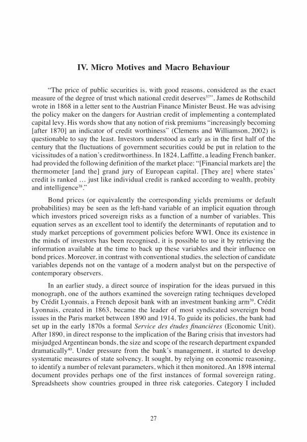
the most creditworthy, category II an intermediate group and category III the leastcreditworthy. Performance parameters are also reported for each country. Becausethe bank used an implicit formula to rank countries, and because this formula exploitedthe information on the performance parameters, one can retrieve the weight of eachparameter in the formula41.

The information retrievable from such exercises depends on the extent to whichindividual ratings and market consensus coincide. The Lyonnais was only one bank— albeit a huge one and for international investment, hugely important — and it wasonly French. What did other investors and intermediaries think, including its British,German, Belgian or Swiss counterparts? To address this question, the individual gradecan be compared with the premium a country had to pay when it sought to borrowabroad. Figure 4 compares the Lyonnais grades with market premiums in 1898. Thegrades were computed using the implicit formula estimated on the basis of theinformation contained in the Lyonnais tables (Flandreau, 2003d). It shows a closeassociation between the individual ratings and “consensus opinion” as reflected bymarket premiums42. Because of archival limitations43, the econometrics are bound tobe somewhat crude44. Nevertheless, the high correlation between individual ratingsand market prices suggests that individual views may be treated as representative ofglobal opinions45. Therefore, looking at what investors looked at can explain a lotabout prevailing views of macroeconomic management. History becomes a guide tounderstand the making of global finance. To a large extent, therefore, Figure 4 representsthis entire monograph in a nutshell. It shows it is possible to work out inductively,from contemporary sources, a number of hypotheses regarding market perceptionsof sovereign risk, and then to test, using bond prices and macro data, whether theseviews are consistent with the pricing of sovereign debt.

This perfectly natural strategy nonetheless implies a fundamental reversal fromstandard approaches and deserves some elaboration. In contrast with the conventionalapproach that relies on Friedman’s “as if” clause (according to which one should usemodern theoretical insights and economic concepts to try to guess what the marketthought), it seeks to infer the pricing of risks from an analysis of actual perceptions.It builds on a reconstruction, from direct observation of the beliefs of contemporaries,of how the market operated and how it weighed risks. The goal is to derive the“model of the world” in the minds of contemporary investors and then use the techniquesof economics to see whether such a model indeed reflected itself in pricing behaviour.This approach is the only practical one to study the features of the prevailingmacroeconomic orthodoxy and, more broadly, the question of expectations, whichplays a decisive role in allocating wealth globally.

29

Dnk USANrw

SwiBel

Nth

Fin

GmySwd

Rus

Tra

ÖstHun

Egy

RomJpn

Ita

Spa

PorGre

ArgSrb

Bra

Lyonnais' score

Yie

ld sp

read

log

Source: d

Le Rentier The Economist

See text. Lyonnais scores computed from Flandreau (2003 ) using an ordered probitmodel. A low grade means a low risk. Yield spreads are computed from monthly bondprices in Paris and London (figures collected from and ).

Figure 4. Individual Beliefs and Market Opinion

0 5 10 15 20 25

1.2

1.0

0.8

0.6

0.4

0.2

0.0

-0.2

-0.4

The basic intuition of this study is to transform the limitation of case studies intoan asset. The study looks for a direct route from microeconomic beliefs to aggregatebehaviour as reflected in bond prices. It requires combining both historical insightsand economic methods. From history, it borrows the need to investigate contemporaryviews carefully before deriving a general model of investors’ perceptions. History byitself would not reveal sufficiently robust lessons on which to base policy prescriptions.Any attempt to infer a general view from one individual source is of course bound tofail, and replication cannot help46. The appropriate technique is not to add a wholelibrary of supporting material on top of a selected reading list. For proofs, the studyturns to the universal techniques of economics. Taking as left-side variables the priceof government bonds and as right-side variables those suggested by an exploration ofindividual sources, it examines whether the beliefs identified in archives can be readfrom the data. This approach, if not conventional, is in the end none othermethodologically than “Cliometrics”, the application of the tools and method ofeconomics to investigate history47.

30

V. What’s on Man’s Mind: Theories in Use

The road crosses beaten tracks. The 19th century notion that sovereign ratespreads measure underlying default risks has stayed alive through the 20th centuryand into 21st century economics. With some formal refinements, the basic intuitionthat interest-rate spreads may be explained or modelled with a variety of factors hasremained48. Recent work has investigated this relation. Factors such as macroeconomicfundamentals, institutions or politics have been considered on top of the gold adherencevariable generally if inappropriately favoured by researchers49. These alternative viewsneed not be exclusive. Macroeconomics might have played a role, just like institutionsand politics. Economists quickly succumbed to the temptation to organise “horse races”to see what view works best50, risking the emergence of an industry of cheap massproduction whose only limit would be data availability. This study’s discussion of therole of theories in use in determining perceived risks warns strongly against theefficiency losses of investing one Euro in this sort of enterprise.

The alternative views on the determinants of bond spreads in fact relate closelyto one another. To interpret regression output properly, one needs clear indications ofhow people gathered and processed information. The problem surfaces when explanatoryvariables get selected. Relying on a mix of more or less rigorously specified modelsand constrained by historical data availability, researchers make compromises that areoften far from satisfactory. Debt-to-GDP ratios provide a characteristic example.Flandreau et al. (1998) pioneered their use to show that fundamentals mattered in theeyes of investors. Obstfeld and Taylor (2003a, 2003b) followed. Yet these ratios haveone big shortcoming. As contemporaries were well aware, nominal debt is a poormeasure of indebtedness. The true burden of the public debt depends on the interestrate at which it is issued, not on its nominal amount51. Contemporaries fully realisedthis and consistently preferred alternative measures. In line with the methodologyadvocated above, one should start from evidence on contemporary beliefs andinformation to identify the variables relevant for market participants. Debt-to-GDPratios might of course have been correlated with something that interested people52,but they were definitely not what people were looking at. The proper route advocatedhere is to identify first the variables that were on people’s minds, then gather them fromcontemporary sources. Only when this is done can one begin to investigate, from whatthe data say, what mattered most in determining bond prices.

This section surveys 19th macroeconomic doctrines. It shows that debt sustainabilitywas the key variable influencing creditworthiness, first because it was a proximatedeterminant of the probability of debt default and second because most other variables(macroeconomic, institutional, political, or other) could be reduced to a public finance problem.The debt burden was a kind of universal unit to which other risks could be reduced.

31

The Debt Burden and Default Risk

An examination of pre-1914 discussions of the factors influencing the probabilityof default immediately reveals considerable concern for what was referred to as the“debt burden”. Applied economists and statisticians emphasised the volume of publicdebts, and market participants echoed them. Baxter (1871) devotes long sections tothe matter. Leroy-Beaulieu’s handbook (1878) has a full chapter on it53. Mulhall’s(1892) statistical dictionary provides a long entry. So did Fenn’s Compendium, theBritish investor reference book first published in the 1830s. The Lyonnais ratingtechniques also gave a lot of emphasis to the debt burden (Flandreau, 2003d). TheInvestor’s Monthly Manual, a companion publication to The Economist, also reportedmeasures of the debt burden. Finally, the conference reports of the Société Internationalede Statistique (between 1887 and 1913) provide several introductions to the problemby Alfred Neymarck (e.g. Neymarck, 1913).

Contemporaries’ main concern was not to prove that debts mattered (everybodyunderstood that they did) but to make sure that their weight would be properly assessed.This involved identifying the best measure of indebtedness and finding a properbenchmark to which it could be compared. Baxter (1871), for instance, describes fouravailable methods. In broad terms, a ratio had to be computed. Choosing the propernumerator proved quite uncontroversial. For the reasons discussed above, nominaldebt was considered inappropriate, and the annual service of the public debt waspreferred. Because public debts typically comprised instruments with very longmaturities, the annual interest service, referred to as “the annuity”, varied little fromyear to year and therefore accurately reflected how much cash had to be paid out “ona permanent basis”.

The identification of the denominator raised more questions. Baxter’s fourthand “most perfect” method related the interest service on the public debt to “the grossincome of the population” (p. 5). As Baxter recognised, this approach (analogous tocomputing debt service-to-GDP ratios) stumbled on the difficulty of obtaining reasonableestimates of national income or, to use a contemporary word, “wealth”54. The problemwould not be fixed until WWI55. The consensus view thus became that national incomeor national wealth estimates were “of a nature more conjectural than scientific, and thesubject of much criticism”56. The prevailing opinion was that “general adoption ofsuch a method had to be left for an age of more complete statistical knowledge”57.

Faute de mieux, a cheap denominator could be population, which was typicallywell documented. Even users of this method systematically pointed out its obviouslimitations58. Two alternative benchmarks thus emerged. One, more widespread andobviously the conventional one around 1900, compared the debt service withgovernment resources. This study will refer to it as the “tax test”. Those who arguedin favour of this ratio emphasised that it closely captured default risks because itfocused on the ability of a given state to service its obligations. The result was ahypothetical relation between probability of default and the variable thus measured.

32

In Leroy-Beaulieu’s words:

“The lower this ratio, the more likely the state is to pay without difficultythe interests on the public debt. …By contrast, when the share [of interestservice] in the total budget is very high, one can fear that the slightestaccident shall put the government in a situation where it is impossible tofulfil its promises”59.

The other approach compared the annuity on the public debt to exports. A briefdescription and defence of it appears in the “Introduction” to the 1889 edition ofFenn’s Compendium, which refers to it as the “trade test”. Because of its lesser scope,and because reference to it disappears in the 1890s, the focus here is on the tax test. Alater section, however, returns to it in a discussion of the economic significance ofalternative methods from the perspective of economic development.

Renegotiation and Memory

The interest service burden was also a crucial variable when default occurred.Unilateral default was always followed by a renegotiation period during which creditorssought to persuade governments to resume interest payments. The ratio that ought tohave been serviced then assumed tremendous importance because it measured creditors’bargaining power. Any increase in the virtual debt burden reduced the likelihood of asettlement palatable for them. Any decrease had the opposite consequence.

Once a default had been settled, a new, reduced, interest service was agreed upon.The country now faced a lower debt burden, but the new ratio actually reflected a worseperformance than it appeared to do. People in the market likely would remember this andinflict penalties on previous defaulters. The Lyonnais ratings show that low debt burdencountries whose “good” prospects had resulted from a failure to meet their obligationswere mechanically downgraded into the infamous “group III” of “junk” nations.The low burden had been achieved not through policy efforts but through repudiation.The debt burden, hanging or not, weighed much on countries’ perceived prospects.

Fiscal and Monetary Variables

Investigation of contemporary sources shows that fiscal and monetary variablesplayed at best a secondary or indirect role, operating through the debt burden ratherthan having an effect of their own. The Lyonnais’ studies did list fiscal performance(computed as the average deficit for a five-year period, thus approximating a“structural” measure) alongside debt-burden measures, but they put little emphasis onit, and its measure made a tiny contribution to overall grades. This can be understoodeasily by recalling that the key issue from investors’ point of view was to determinewhether enough resources could be pledged against the interest-service commitments.In this perspective, a deficit meant, through intensified borrowing, only a marginal

33

increase in interest service in proportion to the resulting increase in the outstandingdebt. If growth or taxation grew more quickly than the public debt, deficits did notmatter. Only in the case of structurally persistent deficits over a long period did fiscalperformance begin to become a worry, but then its influence was identical to that ofan increased debt burden60.

Something similar occurred with monetary factors. The financial press diddocument in much detail note issues, central bank reserves, exchange-rate fluctuationsand exchange-rate regimes. Yet it is not clear from contemporary investors’ perspectivesthat these variables had autonomous influences on perceived risks61. Strictly speaking,faithful adherence to gold as an intrinsic virtue received very little attention in thepre-WWI period62. One does sometimes find quotes praising the gold standard as asuperior regime, but they typically belong at best to the more metaphorical type andat worst to the religious-maniac type discussed in Section III. Given the record availableto contemporary investors, floating currencies tended to display poorer performancesin terms of both economic development and financial probity. The capital-rich countriesof Western Europe had much better records of gold adherence than the capital-poornations on the periphery. That did not mean that floating in itself translated intodowngrades. The “intermediate” group in the Lyonnais risk tables included both floatingand fixed exchange-rate countries, and floating did not appear as an aggravating factor.

Thus, other things being equal, exchange-rate depreciation mattered only to theextent that it resulted from monetary expansion, creating a burden of state liabilitiesthat would have to be paid back. A country that had experienced recurrent public-finance problems and had financed them by printing money or through central bankadvances often ended with a depreciating currency. Return to the pre-float parityrequired repurchasing the excess issue of paper money or repaying the overdraft tothe bank of issue. A standard way to do this was to issue a stabilisation loan63. Sincethis loan would add to the debt burden, a good measure of the “opportunity cost” offloating was to consider the excess money issue as part of the debt burden. Becausefloating currencies often had experienced “excess issues” it is not surprising thatinconvertibility would entail a discount, but it must have been small64.

Similarly, one finds occasional comments that portrayed a large foreign-exchangereserve as a buffer against currency flight. A 100 per cent cover ratio (as in countries suchas Russia after the turn of the century) protected in principle against currency runs, just asmodern currency boards are supposed to do, but foreign loans could provide such coverto governments in need of it. Insurance against exchange-rate volatility could alwaysbe purchased by the fiscally sober. In the end, the gold reserve gave no better guaranteethan sound policy, because credit would be made available to the sound country65.

Currency Clauses and Default Risk

In one instance, however, floating could magnify public-finance problems. Itcould be hazardous when a country had a large external debt denominated in foreigncurrencies and the exchange rate depreciated. Depreciation could then generate servicing

34

difficulties. It led to an increase in interest service that was not necessarily matchedby an increase in nominal tax resources, because taxes revenues lagged66. Between 1890and 1898, Argentina, Portugal, Greece and Brazil all fell into what may be called liquiditycrises through that very channel. Contemporary observers fully understood the danger.As early as 1878, Leroy-Beaulieu warned against the risks of currency depreciationwhen the debt is denominated in foreign currency. His case in point was Russia:

“In the 1876 Russian Empire budget the amount devoted for the interestservice on the public debt was set to 108 418 000 rubles…. By itself, thisnumber was not very large…since it represented only 19 per cent ofexpenditure. However, this weight is most heavy because it has almostentirely been collected abroad. It therefore varies with the course ofexchange. In periods of crises it is likely to rise dramatically. Thus it isinconvertibility which makes the debt burden most importune and painful.Suppose that following concerns or political dangers, or because of adverseeconomic circumstances, the paper ruble, which is legal tender in Russia,depreciates by 20 per cent. This is a 20 per cent increase in the arrears ofthe public debt”67.

This point brings back the question of the exchange-rate regime, but through aquite different channel from the incentive story referred to in Section II. If a fixedexchange rate was to some extent good news for public credit, it did not operatethrough some signalling effect that would have impressed investors, but through aquite material, down-to-earth mechanism whereby exchange-rate depreciation impactedthe soundness of public finances. In contrast, sustained defence of the parity protectedagainst the perils of a run on the public debt, which in turn reverts to the issue of fiscalabstinence. If the external debt was tiny or denominated in domestic currency, muchof the problem disappeared. The challenge, here again, was to be fiscally sober.

The Role of Politics

Politics, domestic and international, obviously mattered in the eyes of contemporaryinvestors. Political crises create uncertainty, and uncertainty drives financial marketsdown. Wars were bad financial news and caused violent fluctuations of bond prices; sodid domestic conflicts such as uprisings or civil wars. Because investors discounted theeffects of political news on the debt burden, they were bound to factor in the consequencesof wars, which always affected the sustainability of public finances. Armed conflictsincreased military expenditures and led governments to borrow (Barro, 1987). Increaseddebts typically followed. When conflict erupted, investors computed the costs ofalternative outcomes, to which they sought to attach probabilities68.

The spread of war indemnities as a routine procedure for victors to financewars ex post compounded the direct effects of wars on public finance. The history ofthe 19th century is replete with these policies: the indemnity of Austria to Prussia in1866, of France to Germany in 1871 and of China to Japan in 1895, to name just the

35

most famous ones. While the victorious country solved any pending public-financeproblems, the defeated one would long bear scars of an increased debt burden thatwould damage its borrowing terms and thus in one way or another its capacity togrow69.

Politics also mattered through reputation. Contemporaries carefully monitoredpolitical regimes. Douglas North’s and Barry Weingast’s now famous analysis (1989)of the British Glorious Revolution of 1688 has popularised the so-called “New Whig”interpretation of the role of democratic institutions (such as parliaments) in fosteringcredibility. Because parliaments committed the sovereign to pay back public debt,they improved borrowing terms and facilitated economic development70. Such views,right or wrong, were perfectly standard a century ago. To illustrate, Laffitte (1824)said that the credit of a state is indeed “ranked according to its wealth” but also “to theinstitutions that guarantee it”. Similarly, Leroy-Beaulieu (1899) argued that “Aparliamentary regime functioning in certain conditions of discipline … and a firmcommitment to established institutions are of course guarantees against financialprodigality”71. In 1863, Adolph Wagner emphasised that a constitution was aprecondition for issuing long-term (perpetual) debt:

“It is not only about financial or material, but more about political guarantees.Only in a constitutional state founded on the rule of law, where an effectiveand independent control of public finances is in place, is there the guaranteefor well ordered public finances and a trustworthy public debt and onlyhere will it be possible to resort to the most rational and healthy form ofpublic debt, the perpetual debt.”

It would not take much effort to provide a boring enumeration. The financialpress and bankers dealing with sovereign risk devoted much time to deciphering thelogic of alternative political regimes and understanding the implications of events.The Economist always commented on political developments with an eye to theirimplications for foreign investors. In Crédit Lyonnais archives one finds a wealth ofnotes discussing the situations of the main political parties, analysing — as for Russia —the risk of potential crises that could threaten the interests of foreign bondholders, andtables describing the principal coalitions running governments72. Yet unlike whatFerguson and Batley (2001) have claimed, it is not clear that politics constituted anindependent factor shaping market views. Rather, in a system where debt sustainabilityis the key variable determining creditworthiness, politics can have an impact on creditthrough their influence on debt dynamics, as the machinery through which the booksare or are not balanced. And there again debt service still features as a crucial variable.

36

VI. Empirical Evidence:Interest Spreads and the Debt Burden

The foregoing survey of contemporary beliefs reveals conclusions at odds withthe modern literature and its considerable (some would say disproportionate) attentionto exchange-rate regimes. They suggest that contemporaries focused mainly on debt-sustainability variables. Investors believed in the debt burden (measured as the ratiobetween debt service and tax revenue) as the key factor influencing debt sustainability— the likelihood of a continued payment of the coupon. In this view of the world, themoney supply, foreign-exchange reserves, fiscal deficits and politics were mostlyintermediary variables. Can one prove this numerically?

The Model

The explanatory variables fall into four groups. The first includes the “structural”factors monitored by contemporary investors. With the debt-to-GDP ratio left aside,the alternative, the ratio of interest service to tax revenues, becomes key. Thepresumption is that this variable was strongly significant and had a large, positiveeffect on interest spreads. Other structural variables monitored by investors andcollected here include the circulation of banknotes, central bank reserves, exports,population and the fiscal deficit. The original, contemporary spreadsheets provide aflavour of the kinds of ratios people contemplated: central banks’ cover ratios, deficit-to-revenue ratios and exports per head73. The likely effects of these ratios on spreadsmight be postulated from contemporary accounts. High cover ratios should reducespreads, and so should high degrees of trade openness74. In contrast, high deficitsshould increase them. On the evidence that people considered such ratios to havesecondary importance, they are not expected a priori to drive the results much. Finally,to capture the feedback from exchange risk to default risk, an asymmetric measure ofexchange-rate volatility, the average depreciation experienced by a given country in agiven year, enables distinguishing between instances of depreciation and of appreciation.A volatile but appreciating currency is not bad news for servicing external obligations,while a volatile but depreciating currency is75.

The second group of variables includes reputation factors. Countries with recentexperience of default should have been downgraded. Investors with memory shouldhave discounted the bonds of those with default records, reducing the penalty as timepassed. Once settlements had occurred, markets should have been prepared to takedefaulters’ bonds again, but at lower prices, other things equal. Moreover, during therenegotiation period that typically followed unilateral default, bonds likely traded at

37

lower prices than otherwise owing to the obvious uncertainty. Investors based theirfundamental assessment of creditworthiness (the probability of recouping capital andinterest) on the “counterfactual” or “virtual” service (i.e. the interest that should havebeen paid, absent default). Yet they certainly also factored in the renegotiation itselfas an aggravating factor until settlement was reached.

The third group comprises political variables. Their identification raises a numberof problems. There seems to have been no simple, consensus definition of what “good”institutions were (beyond the general notion that a well ordered, representativeparliament was preferable to a cruel autocracy) let alone any index to quantify quality,an index whose reconstruction will always suffer from observers’ biases. Identifyingpolitical regimes using modern criteria would obviously not do, and getting a preciseidea of how people related institutions and performance seems difficult. Moreover,because of a relative lack of genuine changes in political regimes over the period understudy, one must give up any hope of using time controls to identify anything. Tocomplicate matters further, political regimes were also broadly associated with economicones. Faithful adherents to the gold standard before 1895 were typically WesternEuropean parliamentary systems (with the possible exception of Italy), which againmakes identification difficult.

Given the lack of consensus on the theoretical relation between political systemsand creditworthiness, the study uses a simple criterion. It focuses on the percentage ofthe population that was enfranchised. Contemporary accounts show that estimates ofthe enfranchised population were in the information set of 19th century investors.Moreover, the broadening of the electoral body had been a recurrent request of theleft throughout the 19th century, and there is evidence that investors closely monitoredits progress. Some scholars have suggested that the limitation of democracy was abasis for the credibility of the pre-1914 gold standard. This predicts a negativeassociation76. This study lets the data decide, but its presumption is that contemporariesthought differently and associated democratic institutions with higher credibility. Thereis evidence that foreign investors encouraged borrowing countries to adoptparliamentary systems. For instance, the Russian finance minister Kokovtsov recountsin his memoirs that after the so-called October Manifesto of 1905, French bankerspressed Russian authorities to give large powers to an elected Duma. They went sofar as to make it a condition for continued lending77. Finally, on top of the proportionof the people that voted, the study considers a wealth of dummies capturing politicalevents such as wars and uprisings.

Last and to a very large extent least, gold adherence is introduced in the regressions.The general framework used here allows testing whether adherence to gold had anyeffect on interest-rate spreads and, if so, how much78. The criterion for gold adherencewas whether the exchange rate remained close enough to the parity during at least sixconsecutive months for a given year, “close enough” meaning “within the gold points”.The conventional defence that changing the precise timing does not alter the results isa matter more of concern than of comfort, and it is not used here. The authors do notfeel compelled to defend further the logic of this variable because they feel a limitedliability toward it. Its contribution is in any case marginal.

38

Readers will find at the end of this study both a long Data Appendix and anequally detailed Technical Appendix. The former serves two main purposes. First, itexplains the variables described above in far greater detail and carefully presents theirsources and derivation. Second, it reproduces the database in its entirety, for use infuture research. The Technical Appendix fully describes both the model and theestimating procedures used, and it presents the results in far greater detail than thosehighlighted below.

Empirical Evidence

The analysis begins by examining the simplest conceivable model, where thevariable to be explained is the interest-rate spread (country i’s interest rate minus theUK interest rate) and the explanatory variables are those reported in the previoussubsection. The model captures the memory effect of past default as an asymptoticallydecaying penalty paid on top of borrowing rates79. A dummy variable correspondingto the period of renegotiation is also used, because the uncertainty surrounding anydebt renegotiation is likely to be considered as an extra cost. The political variables areas described above, and gold adherence is included.

The results reported in Table 1 are simple estimates of the sensitivity of interestspreads to explanatory variables when they are all included together. Alternativeestimates are reported and discussed in the Technical Appendix80. Because capital doesnot flow freely from one country to another — what 19th century economists calledthe “disinclination of capital to migrate” and is today known as the “home bias” — itis useful to document results separately for alternative groups of nations. Table 1therefore provides results for the entire sample, capital-rich countries and capital-poor countries. Because there might have been some changes in the stability ofcoefficients between periods, the Technical Appendix reports results for sub-periods.

Table 1. Determinants of Interest Spreads

All Countries Capital Rich Capital Poor

1. Structural factors : - Interest service/Revenues 7.751 (8.50) 4.144 (6.18) 7.677 (5.35) - Reserves/Banknotes -0.286 (-0.96) 0.223 (1.34) -0.402 (-0.83) - Exports/Population 0.601 (1.59) -0.160 (-1.41) 2.279 (1.95) - Deficit/Tax revenues 0.725 (3.16) 0.319 (1.71) 0.747 (2.21) - Exchange-rate volatility 0.997 (1.14) 2.825 (1.97) 1.310 (1.05)

2. Reputation factors : - Default 4.836 (21.66) - 4.917 (15.48) - Memory 0.703 (2.56) - 0.667 (1.62)

3. Political variables : - Franchise -2.427 (-1.77) -0.839 (-2.17) -7.232 (-1.39) - Political crises F=3.797 (*) F=4.15 (*) F=1.889 (*)

4. Gold adherence: 0.056 (0.32) - 0.099 (0.38) Adj. R2 0.854 0.585 0.798 Number of observations: 480. Not shown are the country-specific constants. (*) = F-test significant at 5 per cent.

39

Table 1 points to a number of findings. It outlines the overarching importance ofthe debt burden. It implies that on average, a 10 per cent rise in the debt burden (e.g. arise of the debt service from 20 to 30 per cent of government revenue) increasedborrowing rates by 70 to 80 basis points. This contrasts with the other explanatoryvariables, such as the cover ratio, the deficit ratio or the openness ratio, which getmuch less credit. While generally correctly signed81, they have little impact on interest-rate spreads and are rarely significant, a finding consistent across the groups of countries.These results support the approach suggested here. They reveal the interest burden as anessential variable for investors; it drove perceptions of macroeconomic stability.

Default variables are also strongly significant. When debt renegotiation occurred,spreads went up by about 500 basis points. Once settlement was reached, a penalty ofabout 90 points was paid the first year, and it was still at 45 basis points ten yearslater. Just as observed in the study of individual ratings, markets did remember.Combined with the significance of the debt burden, this result is fully consistent withthe rating formulas discussed in previous sections. In the end, the debt burden anddebt default appear to explain most of the variance of interest-rate spreads. Thesignificance of previous defaults in determining borrowing conditions may also helpto reconcile the intuitive notion that investors should remember with the popularclaim that markets do not remember. While there is indeed a penalty for defaulting, itturns out over the medium term to be of a smaller order of magnitude than the savingsassociated with the debt repudiation. Governments had a clear incentive for notrepudiating their debt, but it was too small to act as a systematic deterrent.

Table 1 shows the exchange depreciation variable as non-significant. Resultsreported in the Technical Appendix for alternative specifications show it with moresignificance and generally with greater effects for capital-poor countries, which theprevious section argued were more vulnerable to “twin” crises because of their largeexposure to debt denominated in foreign currency. In fact, as the Appendix also shows,the introduction of the political crisis dummies swamps the significance of the exchange-rate vulnerability variable. This is quite understandable but also very important, becauseexchange crises are often triggered by political crises. Political uncertainty, whichappears as the one significant factor besides the debt burden and debt default, oftenmagnified financial crises and exchange-rate vulnerability. In contrast, the extensionof the suffrage does not show up in the regressions reported in Table 1. Note, however,that it becomes significant in some of the regressions shown in the Appendix and willagain surface in an alternative model.

Finally, the gold variable is never significant. In fact, as shown in the Appendix,its effect is not stable across equations, especially when one considers various groupsor, even more strikingly, sub-periods, when it sometimes comes up with the “wrong”sign. Gold adherence works well only when an analysis gives it a kind of monopolypower. When it must compete with a few other variables, especially the debt-defaultvariables but also the political-crisis variable, its effect declines or vanishes82. Thegold dummy might simply tell us, when it comes out with the “expected” negativeand significant sign, that a country in crisis is a country in crisis.

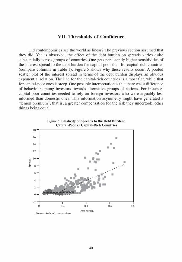
40

VII. Thresholds of Confidence

Did contemporaries see the world as linear? The previous section assumed thatthey did. Yet as observed, the effect of the debt burden on spreads varies quitesubstantially across groups of countries. One gets persistently higher sensitivities ofthe interest spread to the debt burden for capital-poor than for capital-rich countries(compare columns in Table 1). Figure 5 shows why these results occur. A pooledscatter plot of the interest spread in terms of the debt burden displays an obviousexponential relation. The line for the capital-rich countries is almost flat, while thatfor capital-poor ones is steep. One possible interpretation is that there was a differenceof behaviour among investors towards alternative groups of nations. For instance,capital-poor countries needed to rely on foreign investors who were arguably lessinformed than domestic ones. This information asymmetry might have generated a“lemon premium”, that is, a greater compensation for the risk they undertook, otherthings being equal.

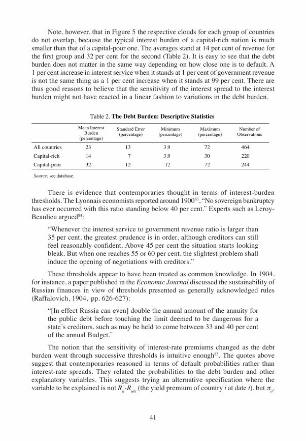
41

Note, however, that in Figure 5 the respective clouds for each group of countriesdo not overlap, because the typical interest burden of a capital-rich nation is muchsmaller than that of a capital-poor one. The averages stand at 14 per cent of revenue forthe first group and 32 per cent for the second (Table 2). It is easy to see that the debtburden does not matter in the same way depending on how close one is to default. A1 per cent increase in interest service when it stands at 1 per cent of government revenueis not the same thing as a 1 per cent increase when it stands at 99 per cent. There arethus good reasons to believe that the sensitivity of the interest spread to the interestburden might not have reacted in a linear fashion to variations in the debt burden.

Table 2. The Debt Burden: Descriptive Statistics

Mean InterestBurden

(percentage)

Standard Error(percentage)

Minimum(percentage)

Maximum(percentage)

Number ofObservations

All countries 23 13 3.9 72 464Capital-rich 14 7 3.9 30 220Capital-poor 32 12 12 72 244

Source: see database.

There is evidence that contemporaries thought in terms of interest-burdenthresholds. The Lyonnais economists reported around 190083, “No sovereign bankruptcyhas ever occurred with this ratio standing below 40 per cent.” Experts such as Leroy-Beaulieu argued84:

“Whenever the interest service to government revenue ratio is larger than35 per cent, the greatest prudence is in order, although creditors can stillfeel reasonably confident. Above 45 per cent the situation starts lookingbleak. But when one reaches 55 or 60 per cent, the slightest problem shallinduce the opening of negotiations with creditors.”

These thresholds appear to have been treated as common knowledge. In 1904,for instance, a paper published in the Economic Journal discussed the sustainability ofRussian finances in view of thresholds presented as generally acknowledged rules(Raffalovich, 1904, pp. 626-627):

“[In effect Russia can even] double the annual amount of the annuity forthe public debt before touching the limit deemed to be dangerous for astate’s creditors, such as may be held to come between 33 and 40 per centof the annual Budget.”

The notion that the sensitivity of interest-rate premiums changed as the debtburden went through successive thresholds is intuitive enough85. The quotes abovesuggest that contemporaries reasoned in terms of default probabilities rather thaninterest-rate spreads. They related the probabilities to the debt burden and otherexplanatory variables. This suggests trying an alternative specification where thevariable to be explained is not Rit-Rukt (the yield premium of country i at date t), but πit,

42

the default probability. The relation between the two is straightforward and, as it turnsout, non-linear86. Nevertheless, as Figure 6 reveals, a pooled scatter plot of the probabilityof default in terms of the debt burden actually displays a linear pattern; formal tests onthe stability of coefficients across sub-groups can confirm this impression. Theimplication is that moving from yield premiums to default probabilities enables one tolinearise the relations under study.

Finally it is possible to back up the theoretical relation between the debt burdenand interest-rate spreads. This is shown in Figure 7, which is constructed using theelasticity of default probability to the debt burden reported in Table 3. The figureresembles Figure 5. Because the British rate enters the formula for the default probability,various curves correspond to various British rates. Ceteris paribus, spreads increasedwhen the British rate increased. The figure also suggests that the sensitivity of interestspreads to the debt burden rose markedly when the debt burden approached andpassed 40 per cent of tax revenues. This confirms the non-linearity and contemporarycomments about threshold effects.

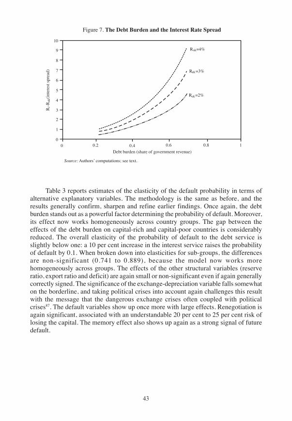
43

R =4%

R =3%

R =2%

R -R

(in

tere

st sp

read

)10

9

8

7

6

5

4

3

2

1

00 0.2 0.4 0.6 0.8 1

Debt burden (share of government revenue)

Source: Authors’ computations; see text.

Figure 7. The Debt Burden and the Interest Rate Spread

uki

uk

uk

uk

Table 3 reports estimates of the elasticity of the default probability in terms ofalternative explanatory variables. The methodology is the same as before, and theresults generally confirm, sharpen and refine earlier findings. Once again, the debtburden stands out as a powerful factor determining the probability of default. Moreover,its effect now works homogeneously across country groups. The gap between theeffects of the debt burden on capital-rich and capital-poor countries is considerablyreduced. The overall elasticity of the probability of default to the debt service isslightly below one: a 10 per cent increase in the interest service raises the probabilityof default by 0.1. When broken down into elasticities for sub-groups, the differencesare non-significant (0.741 to 0.889), because the model now works morehomogeneously across groups. The effects of the other structural variables (reserveratio, export ratio and deficit) are again small or non-significant even if again generallycorrectly signed. The significance of the exchange-depreciation variable falls somewhaton the borderline, and taking political crises into account again challenges this resultwith the message that the dangerous exchange crises often coupled with politicalcrises87. The default variables show up once more with large effects. Renegotiation isagain significant, associated with an understandable 20 per cent to 25 per cent risk oflosing the capital. The memory effect also shows up again as a strong signal of futuredefault.

44

Table 3. Determinants of Default Probabilities

All Countries Capital-Rich Capital-Poor

1. Structural factors : - Interest service/Revenues 0.847 (10.60) 0.889 (4.31) 0.741 (7.19) - Reserves/banknotes 0.014 (0.53) 0.080 (1.76) -0.021 (-0.60) - Exports/Population 0.016 (0.48) -0.032 (-1.02) 0.134 (1.60) - Deficit/Tax revenues 0.001 (0.07) 0.095 (1.86) -0.015 (-0.61) - Exchange rate volatility 0.143 (1.89) 0.801 (2.04) 0.163 (1.82)

2. Reputation factors : - Default 0.164 (8.49) - 0.178 (7.78) - Memory 0.134 (5.61) - 0.110 (3.70)

3. Political variables : - Franchise -0.548 (-4.64) -0.302 (-2.85) -1.301 (-3.48) - Political crises F=3.088 (*) F=4.83 (*) F=1.928 (*)

4. Gold adherence: -0.040 (-2.61) - -0.028 (-1.54) Adj. R2 0.859 0.527 0.758 Number of observations: 480. Not shown are the country-specific constants. (*)=F-test significant at 5 per cent.

The only substantial change from the previous results is that the extension ofthe suffrage now reduces the probability of default quite substantially. The effect ofan increase in the enfranchised population from 0 to 25 per cent (as would typicallyhave occurred through extending the suffrage to the adult male population at the turnof the century) reduces the probability of default by a considerable 0.125. This isconsistent with the notion alluded to earlier that contemporaries saw democracy andparliaments as a source of greater stability, because they put checks and controls onthe sovereign. This raises some intriguing questions in view of more recent research.If anything, the findings here suggest that the expansion of democracy, not itsrestriction, promoted financial stability during the period by facilitating internationalborrowing through lowered premiums. This contradicts the widespread view that therepression of democracy facilitated the operation of the pre-1914 international monetarysystem by making the external adjustment easier88.

Finally, gold adherence again shows up as a borderline variable, non-significantwhen more explanatory variables are included. This residual effect is fully consistentwith the view that a floating currency penalised countries to the extent that investorsunderstood that excess paper money would have to be absorbed through internationalloans. But gold adherence, as such, was hardly a rewarding badge to wear. If onewanted to minimise the cost of borrowing, a low debt burden, a commitment totimely payment of coupons, a swift settlement if default occurred, more democracyand political and diplomatic stability were much more relevant than continued adherenceto the gold standard. Investors could see through the veil of monetary regimes.

45

VIII. Convergence Explained

It now becomes possible to put together the findings and provide a comprehensiveinterpretation of the convergence of interest rates before WWI. As abundantlydocumented in previous sections, fluctuation in debt burdens was the backbone oflong-term interest-rate movements. Hence, the convergence of yield premiums beforeWWI must have been related to a dramatic reduction of those burdens. Figure 8 illustratesthis by showing the association between interest-rate convergence (reductions in interestspreads) and improved debt sustainability (reduction in debt burdens). The chart focuseson non-defaulters in order to purge the data from possible biases in favour of thisclaim89. It displays a striking association between the two processes. On average, areduction of the debt burden by 5 per cent (e.g. a reduction of interest service from20 per cent to 15 per cent of tax receipts) reduces the interest spread by 50 basispoints. The story thus unfolds. Investors monitored debt burdens, which were reduceddramatically. They thus concluded that the world was turning into a much safer placefinancially and became increasingly more eager to lend abroad. This explains theastonishing degree of financial integration reached before WWI.

Redu

ctio

n in

deb

t bur

den

(frac

tion

of ta

xes)

0.25

0.2

0.15

0.1

0.05

0.0

-0.050

Reduction in spreads (1880 to 1913)Source: See text and Statistical Appendix.

0.5 1 1.5 2

Figure 8. Lower, Safer

46

Fully documenting why debt burdens declined would go somewhat beyond theboundaries of the present monograph, which focuses on the supply side (the marketmechanism) more than on the demand side (governments’ borrowing policies). Someremarks are nonetheless in order. The dynamics of the debt burden can be brokendown into a list of elementary components. On the one hand annual interest serviceincreased with additions to the public debt. On the other, tax revenues rose; the sourcesof the rise can themselves be decomposed into economic growth, the scope of taxation(the extent of the tax ratio) and inflation. Higher growth, increased taxation or higherinflation all reduce the debt burden, other things being equal90.

Figure 9 provides a decomposition of the sources of the reduction in debt burdens.It displays the annualised average growth rates of the various components of the debtburden dynamics: debt service, growth rates, increases in taxation and inflation91. Factorsthat deteriorated (i.e. increased) debt burdens bear a negative sign. Declines in publicdebt did not drive the reductions in debt burden in many cases, and gross debt servicekept rising across time for most countries in the sample. In fact, public debts oftenclimbed steadily throughout most of the period under study92, but the dynamics of theother items more than compensated for this. Leaving aside inflation as a mostlyexogenous variable during the period93, the extension of taxation and growth are leftas the main potential sources of international financial integration. Because the extensionof taxation remained quite limited, growth was the chief factor offsetting the increasesin public debt. It therefore served as the modus operandi in the financial markets acentury ago, causing international financial integration. The period’s favourableeconomic performance essentially propelled the process of globalisation.

The first great era of globalisation did not succeed because it displayed aparticularly high commitment of governments to sound finances. In that respect theperiod was just as unexceptional as any other. Rather, success came because fairlyremarkable economic growth characterised the times. Because this conclusion movesaway from the realm of financial and monetary rules to problems of development, itseriously qualifies the conventional view that globalisation owed much to the gold-standard ethos. The question is whether contemporaries realised that, or if insteadthey only mechanically priced sovereign risk through the abstract formula identifiedhere. The next section discusses this issue and explores the relations between riskperceptions and development policies.

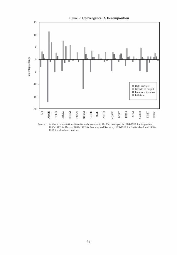
47

AH

ARG

E

BELG

BRA

Z

DEN

M

FRA

N

GER

M

GRE

E

ITA

L

NET

H

NO

RW

PORT

RUSS

SPA

I

SWED

UN

IK

Debt serviceGrowth of outputIncreased taxationInflation

15

10

5

0

-5

-10

-15

-20

Perc

enta

ge c

hang

e

Source: Authors' computations from formula in endnote 90. The time span is 1884-1912 for Argentina,1885-1912 for Russia, 1881-1912 for Norway and Sweden, 1899-1912 for Switzerland and 1880-1912 for all other countries.

Figure 9. Convergence: A Decomposition

SWIT

48

IX. Developmental Consequences

A crucial element has come to the fore. This study’s interpretation of the mechanicsof interest-rate convergence underlines the importance of growth and development inachieving a sustained reduction of borrowing prices. This is natural because over thelong run the ability to service public debt relates ultimately to the adoption of policiesthat foster economic development. This section argues that there was a one-for-onecorrespondence between the assessment of sovereign risks and contemporary thinkingon development strategies. If, as shown here, gold adherence played little role inshaping pre-1914 reputations, elaboration is needed on the stuff of which they actuallywere made. The analysis returns to the risk-assessment techniques reviewed in SectionV and discusses the economics of the “trade test” and “tax test”, which weighed thedebt burden against national exports and government revenues. These alternative criteriacorresponded to successive views on governance and development. While the tradetest emphasised export promotion (and thus laissez-faire) the tax test stressed efficientfiscal and economic management (and thus to some extent government intervention).The watershed for the emergence of the tax test as a norm was the 1890 Baring crisis,which revealed the importance of good fiscal governance.

Openness, Development and the Trade Test (1848-1889)

The 1889 edition of Fenn’s Compendium (pp. xix-xx) provides the most articulatepresentation of the trade test. The editor, Robert Lucas Nash, explains its rationale byarguing that trade openness was the single most important variable to denote prosperity:

“There is perhaps no better test of a nation’s wealth than its foreign tradefor, as a rule, countries which are rich have those things which other nationscovet, and countries which are poor have not.”

As later developed for the tax test, Nash further suggested thresholds that wouldenable identification of delinquent countries. Reasoning in terms of the “volume ofthe debt” which he computed by capitalising the interest-service annuity using a 5 percent interest rate and dividing it by exports, Nash identified a danger zone lying abovefour (equivalent to a ratio of the debt service to exports equal to 20 per cent as explainedin note 94)94:

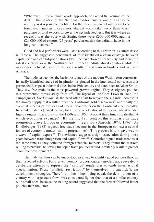
49

“Wherever … the annual exports approach, or exceed the volume of thedebt … the position of the National creditor must be one of as absolutesecurity as it is possible to obtain. Further than this, no defaulters are to befound even amongst those states where it would take two or three years’purchase of total exports to cover the net indebtedness. But it is where asrecently was the case with Spain, there were £500 000 000, against£20 000 000 of exports (25 years’ purchase), that the defaults have in thelong run occurred.”

Good and bad performers were listed according to this criterion, as summarisedin Table 4. The suggested benchmark of four identified a clean cleavage betweencapital-rich and capital-poor nations (with the exception of France).By and large, thesafest countries were the Northwestern European industrialised countries while therisky ones included those on Europe’s southern and eastern borders and in LatinAmerica.

The trade test echoes the basic postulates of the modern Washington consensus.Its easily identified source of inspiration originated in the intellectual consensus thatpermeated European industrial elites in the 19th century and dates back to Adam Smith.They saw free trade as the most powerful growth engine. They castigated policiesthat represented moves away from it95. The repeal of the Corn Laws in 1846, thecampaigns of The Economist, the need after 1848 to recycle the gigantic increase inthe money supply that resulted from the California gold discoveries96 and finally theeventual success of the ideas of liberal economists on the Continent (the so-calledfree-trade epidemic) paved the way for a drastic acceleration of European trade. Availablefigures suggest that it grew in the 1850s and 1860s at about three times the rhythm atwhich economies expanded97. By the mid-19th century, this emphasis on tradepromotion drove European economic integration (Bairoch, 1974, 1976). AsKindleberger (1988) argued, free trade became in the European context a centralfeature of economic modernisation programmes98. This process in turn gave way toa wave of capital exports99. The evidence suggests a tight association during thoseyears between trade integration and capital flows100. Countries signed trade treaties atthe same time as they solicited foreign financial markets. They found the marketswilling to provide, believing that open trade policies would inevitably result in greatereconomic development101.

The trade test thus can be understood as a way to identify good policies throughtheir revealed effects. For a given country, proportionately modest trade revealed adeliberate attempt to repress the “natural” tendencies towards internationalspecialisation. These “artificial restrictions” by themselves indicated deficientdevelopment strategies. Therefore, other things being equal, the debt burden of acountry with large trade flows was considered lighter than that of a similar countrywith small ones, because the trading record suggested that the former followed betterpolicies than the latter.

50

Table 4. The Trade Test Circa 1888

(1) Net Debt

Capitalised at 5% (£ millions)

(2) Net Debt (£/head)

(3) Annual Exports

(£/head)

(4) Ratio: (2)/(3)

United Kingdom 396 10.58 7.50 1.41 Austria-Hungary 465 11.36 1.75 6.49 Belgium 63 4.11 16.65 0.25 France 986 23.90 3.48 6.88 Prussia 180 - 4.75 - Greece 28 14.65 1.73 8.49 Italy 430 13.25 1.45 9.14 Netherlands 52 10.11 17.95 0.56 Norway 5 1.13 2.95 0.38 Portugal 79 16.75 1.21 13.81 Spain 202 11.73 1.63 7.22 Sweden 11 0.68 2.91 0.23 Russia 535 4.91 0.75 6.55 Argentine Republic 85 21.40 4.00 5.35 Brazil 98 7.30 1.58 4.63 Notes: The net public debt is obtained by subtracting interest on liabilities backed by assets (railways etc.) from total

interest payments. The result is then capitalised using a uniform interest rate of 5 per cent. Fenn’s Compendium reports Austria and Hungary separately for debt but aggregated for trade. The debt numbers are aggregated here to permit comparison. Fenn’s Compendium apparently lacks data for Germany, but “Prussia” might be understood as a proxy (note alphabetical order). It is not clear to what trade (German or Prussian) the number in column (3) refers.

Source: From Fenn’s Compendium, 1889, p. XV.

The Tax Test and Financial Development (1890-1914)

After 1890, reference to the trade test disappears from subsequent editions ofFenn’s Compendium and the related literature. More and more references to the taxtest start appearing. This reflected a change in development views and strategies.

As economic historians noted long ago, the 19th century’s later developers insouthern and eastern Europe tended to use the state to promote economic development.This observation is traditionally associated with Gerschenkron’s thesis on “economicbackwardness”102. Typically, public loans funded infrastructure — roads, canals,railways. The tax test in many respects seems to have been tailored for such countries.While public investment projects typically increased the interest service over the shortrun, they also improved prospects for future revenues and thus led to an eventualupgrading of fiscal resources through two different channels. First, to the extent thatstate projects were well run and well managed, they generated flows of “dividends”that alleviated or annihilated the corresponding debt service103. Second, more

51

infrastructure spurred growth and regional specialisation. Both improved public financesby increasing and broadening the tax base and thus favouring the collection ofgovernment revenue. States that actively promoted domestic development undertooksteps that eventually affected the behaviour of the tax test.

In this respect the tax test was a way to focus on the success of governmentpolicies. It led observers to consider efficiency in the collection of taxes, to track theimpacts on fiscal performance of centralisation, corruption or the training of taxcollectors104. It led them to study the effects of financing development throughalternative taxes, such as customs duties, excises, income taxes and stamp duties.One could also monitor the management of state companies and monopolies throughthe tax test because their creation and operation affected the behaviour of both theinterest burden and government revenues. The tax test was a means to understandbetter the operation of the fiscal machinery.

Starting in the late 1880s, extensive evidence of attention to these problemsappears in contemporary accounts. One typical illustration involved the frequentattempts to discount “reproductive investment” from the public debt105. As manyobservers recognised, establishing rigorous accounts of the debt burden, which wouldalso enable discrimination between productive and unproductive debts, was bothtremendously difficult and very important106. Sorting out these technical problemsbecame a major challenge for investors, who devoted much time and energy to it.Such concerns became a key feature of the Crédit Lyonnais country reports, inevitablyleading to comments on the relative abilities of states to promote national development.The reports of the Council of Foreign Bondholders carefully discounted productivedebts from total debts107. The tax test thus led to discussions of governance108. Inblatant contradiction with the popular belief that the late 19th century system restedon laissez-faire, during most of the period after about 1890 the assessment of defaultrisks was rooted in a view that placed much emphasis on the ability of governments tomanage their economies in ways that would foster their own fiscal resilience. “Good”policies were those that successfully struck a balance between fiscal developmentand national economic growth.

The Argentine Crisis as a Watershed

While the trade test corresponded closely in both timing and spirit to the firstphase of 19th century globalisation (1848-1889), which mostly involved WesternEuropean integration, the tax test best fitted the experience of later developers withtheir experience of “hands on” government (1889-1913)109. It is tempting to stress theopposition between the trade and tax tests, but this would be somewhat inappropriatebecause the criteria were not mutually exclusive. Results in Sections VI and VII displayevidence that openness mattered. Supporters of the trade test, such as Fenn’sCompendium, did also acknowledge the high relevance of the quality of public spending.Finally, for all practical purposes, a stable empirical relation does exist, for a given

52

country, between taxation as a share of GDP and openness110. The Technical Appendixto this study reports results from regressions using both criteria111. The two criteriashow very similar explanatory power for the overall sample.

To highlight the differences between the tests, Figure 10 provides a cross-sectionof the scores obtained by the countries in the sample in 1888112. A relation does existbetween them; it explains their comparable overall records. The shaded rectangle,which is the intersection of the “danger zones” according to both tests, captures theusual suspects — in alphabetical order, Argentina, Greece, Italy and Portugal. Braziland Spain are on the border. Note, however, that three high-risk countries, Argentina,Brazil and Greece, lie to the right of the adjustment curve. Together with Portugal (alooming disaster according to both tests) these countries were the ones that went bustin the 1890s. While recognised as highly hazardous under both criteria, they hadbleaker prospects according to the tax test113.

Figure 10. Trade and Tax Tests in 1888

Source: Fenn's CompendiumDatabase and as reported in Table 4.

Portugal

Italy

SpainGreece

Argentina

Brazil

16

14

12

10

8

6

4

2

00 0.1 0.2 0.3 0.4 0.5

Tax test: interest service on public debt divided by government revenue

Trad

e te

st fr

omca

pita

lised

inte

rest

serv

ice

onpu

blic

deb

t div

ided

by

expo

rtsFe

nn's

Com

pend

ium

:

As a matter of fact, the Argentine collapse in 1890 was the watershed thatcaused the emergence of the tax test as the key criterion. To see this, consider whatought to have been the interest premiums paid by Argentina in the 1880s on the basisof the relation between debt burdens and interest spreads as it emerged after the

53

crisis. One can estimate the basic model on 1900-13 using both the trade and taxtests, then simulate the spreads one gets according to each criterion. The result isshown in Figure 11, which compares the observed spread with the simulated ones.The trade test fits the actual rate quite well, suggesting that such a criterion wasindeed used in the 1880s. The tax test, by contrast, shows how much the marketswould have charged if they had priced the Argentine debt as they did in the 1900s.This alternative predicts a substantially higher interest spread, and it tends to increaseas the crisis approaches, reaching 200 basis points in 1889. Obviously, a greateremphasis on the tax test might have led to a limitation on Argentine borrowing. Thesubsequent crises in Greece, Portugal and Brazil may therefore be understood in thislight. The Argentine collapse led investors to monitor public finances and debt burdensmore carefully. They realised that some countries, while possibly very open (Brazil),had deeply deficient fiscal systems. The Argentine wake-up call led investors toreconsider the hierarchy of risks in the light of Argentina’s problems. The CréditLyonnais, for one, began carefully measuring interest burdens. The Council of ForeignBondholders did the same. When the “bad performers” according to this criterionfound themselves in trouble and sought to borrow, they did not find capital andcollapsed114.

6.5

6.0

5.5

5.0

4.5

4.0

3.5

3.0

2.5

2.01884 1885 1886 1887 1888 1889 1890

Observed

Simulated trade test

Simulated tax test

Figure 11. Forecasting Disasters: Alternative Measures

Source: See text. Fixed effects model estimated for 1900-1913. Simulation usingthe Argentine data from the Statistical Appendix.

Spre

ads

54

If this interpretation holds, one can understand the decline of popularity of thetrade test and growing use of the financial-burden method thereafter115. This analysisunderlines the links between assessment of sovereign risks and development views. Itsuggests that the international financial markets of the 19th century, while rewardingtrade openness, became increasingly concerned about the very quality of financialpolicies. In the end, everything happened as if capital mobility had magnified thefocus on individual financial achievements and led investors to realise that internationaleconomic integration created hazards (Calvo, 2003). As globalisation extended itsreach beyond Western Europe to the broader world, people discerned that integrationhad been embedded in a much deeper fabric than the mere focus on trade opennesshad incorrectly suggested. This in turn gradually provided a new definition of what“good” policies were and magnified in this light the importance of sound fiscalmachinery (an old feature of modern European states). People came to understand thatdealing with globalisation required appropriate financial policies much more than thesimple pursuit of free trade. The present epoch, it seems, is only relearning this lesson.

55

X. Policy Lessons and Conclusions

This monograph has sought to trace the roots of global financial integration inthe first “modern” era of globalisation. It has shown that this integration, as measuredby standard indicators, was not a monotonic process. A first wave of financial integrationlasted until the 1880s, and a second one occurred in the early 1900s. This rules out adriving role for improvements in financial technology116. The interpretation focusedinstead on supply factors — perceptions by investors of the quality of the policies thatborrowing countries followed. These perceptions shaped views regarding the relevantparameters people ought to monitor. As a result, investors “priced” government actionson the global capital market, because government securities were traded at levels thatreflected the degree of trust they inspired. A deterioration of sovereign risk due to theperceived deterioration of a country’s macroeconomic policies led investors to chargea premium for new loans, thus limiting the extent to which countries got access tointernational capital. This was especially problematic for developing or “capital-poor”countries, because, for them, access to international finance was paramount. Oneimportant conclusion is that formally removing capital controls is not enough forachieving a high degree of financial integration. The liberalisation of the capital accountis at best a necessary but not sufficient condition for integration. Reputation is the truedriver.

The interpretation of the sources of financial integration put forward hereunderlines the importance of domestic policies in actually facilitating the globalcirculation of capital. By emphasising the role of market processes, it answers thedebate (see Bayoumi, 1990) on whether financial integration results from governmentpolicies or from some “endogenous” market behaviour. This contrasts sharply withthe reading of globalisation put forward by Obstfeld and Taylor (1998), according towhich policies affecting financial openness (removal of capital controls, etc.) propelthe ebbs and flows of international financial integration. It has shown that policiesreducing the perception of risks by the market are the true forces facilitating thecirculation of capital. The adoption of “good” domestic policies expedites theglobalisation of capital much more decisively than does the removal of legal barriersto financial exchange.

This points to an essential lesson for developing countries. Because sovereigndebt stands in the front line when investors set a benchmark for the risk of lending toany given country, how they assess it is liable to play a decisive role in determininghow much foreign capital that country can attract. This decisive element of the logicof international financial integration, surprisingly, has received only neglect in recentdiscussions of international financial integration117. Yet the recent troubles in whichdeveloping countries find themselves when they seek to attract foreign capital suggeststhat such forces prove decisive.

56

To identify the perceptions relevant for late 19th century investors, thismonograph gathered material from individual sources in order to establish a list ofpotential candidates. Relying on a new database collected from primary sources, itsought to test whether the economic perceptions of the time were indeed reflected in“market prices”. It related alternative measures of default risk to such variables as thedebt burden, the cover ratio of the central bank, the deficit ratio, trade openness,default, past default, political regimes, political crises and exchange-rate regimes.Two alternative models were considered. One sought to explain interest-rate differentialswith England (model I). The other sought to explain default probabilities (model II).In both cases the right-hand variables were the candidates identified above. Model IIwas shown to be preferable in many respects. It provided an elegant way to handle“threshold effects”, i.e. markets getting the jitters when some performance parametersdeteriorate relative to consensus-determined benchmarks.

The empirical findings show a hierarchy among explanatory variables. First,they reject the conventional view that the exchange-rate regime (participation in thegold standard) mattered in facilitating the global circulation of capital118. Theydemonstrate that such a conclusion is flawed and can result only from mis-specificationand mis-measurement. Its significance in earlier studies comes from a general neglectof other variables that, in fact, people monitored carefully, as they should have. Thisstudy finds participation in the gold standard, even when statistically significant indetermining borrowing terms, to be only marginally so with a small effect. Moreover,it explains a mediocre part at best of the convergence of interest-rate spreads after1900 and of the resulting capital market globalisation. The gold standard was not thebasis of the first era of financial globalisation.

Second, the debt burden was the one key variable that determined market access,because to a large extent it captured and summarised many macroeconomic features.Provided that a country had a low debt burden, it could finance its deficit withoutproblem — the deficit itself often did not show up as a significant variable. A countrywith a low debt burden could borrow reserves to shore up its currency — and theexchange-rate regime had little if any effect.

That monetary regime variables did not appear as significant while the debtburden did suggests that to a large extent there was a disconnection, even beforeWWI, between the exchange-rate regime and globalisation119. Only when countriessuffered from “original sin”, i.e. when they could not borrow in their own currencies120

and thus accumulated large currency exposures, could the exchange regime matter.Exchange crises when countries had large debts denominated in foreign currenciescould be deadly. This led them to find ways to mitigate the fluctuation of their exchangerates or to seek to reduce their exposure to currency risk by encouraging the developmentof deep domestic markets to which foreigners could come. Hard pegs offered anoption, of course, and some countries such as Russia adopted them. Yet gold adherenceof the currency-board type acted not as a signal for good policies, but as insuranceagainst the so-called “twin crises”. The choice of exchange-rate regime was more aconsequence than a cause of globalisation. This conclusion remains valid.

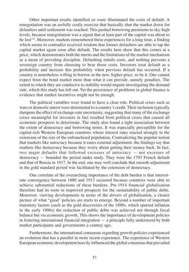
57

Other important results identified en route illuminated the costs of default. Arenegotiation was an awfully costly exercise that basically shut the market down fordefaulters until settlement was reached. This pushed borrowing premiums to sky-highlevels, because renegotiation was a signal that at least part of the capital was about tobe lost121. Moreover, markets remembered these experiences for a long time, a findingwhich seems to contradict received wisdom that former defaulters are able to tap thecapital market again soon after default. The results here show that this comes at aprice, which demonstrates both the merits and the limitations of the market mechanismas a mean of providing discipline. Defaulting entails costs, and nothing prevents asovereign country from choosing to bear those costs. Investors treat default as aprobability and increase this probability when previous default has occurred. If acountry is nonetheless willing to borrow at the new, higher price, so be it. One cannotexpect from the bond market more than what it can provide, namely penalties. Theextent to which they are conducive to stability would require investigating the demandside, which this study has left out. Yet the persistence of problems in global finance isevidence that market incentives might not be enough.

The political variables were found to have a clear role. Political crises such aswars or domestic unrest were detrimental to a country’s credit. Their inclusion typicallydampens the effect of exchange-rate uncertainty, suggesting that many of the exchangecrises meaningful for investors in fact resulted from political crises that caused alleconomic prospects to deteriorate. The study also found a tight association betweenthe extent of democracy and borrowing terms. It was especially perceptible for thecapital-rich Western European countries whose interest rates reacted strongly to theextension of the size of the enfranchised population. Contradicting the popular notionthat markets like autocracy because it eases external adjustment, the findings say thatmarkets like democracy because they worry about getting their money back. In fact,two major defaults that followed excesses of autocracy — not excesses ofdemocracy — bounded the period under study. They were the 1793 French defaultand that of Russia in 1917. In the end, one may well conclude that smooth adjustmentin the gold standard period was facilitated by the extension of democracy.

One correlate of the overarching importance of the debt burden is that interest-rate convergence between 1880 and 1913 occurred because countries were able toachieve substantial reductions of these burdens. Pre-1914 financial globalisationtherefore had its roots in improved prospects for the sustainability of public debts.Moreover, viewing developments in terms of the drivers of globalisation, a clearerpicture of what “good” policies are starts to emerge. Beyond a number of importanttransitory factors (such as the gold discoveries of the 1890s, which spurred inflationin the early 1900s) the reduction of public debts was achieved not through fiscalbalance but via economic growth. This shows the importance of development policiesin fostering international financial integration — a principle fully understood by bothmarket participants and governments a century ago.

Furthermore, the international consensus regarding growth policies experiencedan evolution that has a parallel in more recent experience. The experience of WesternEuropean economic development heavily influenced the global consensus that prevailed

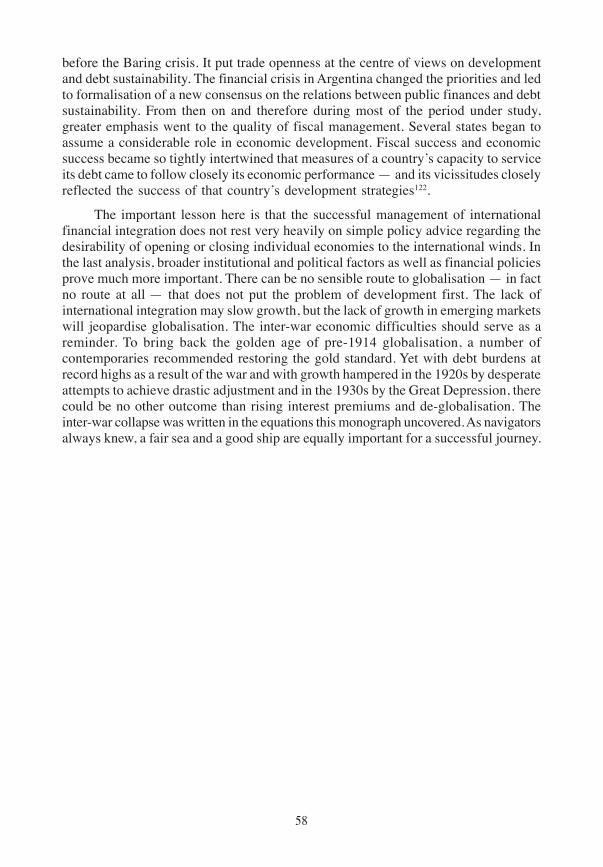
58

before the Baring crisis. It put trade openness at the centre of views on developmentand debt sustainability. The financial crisis in Argentina changed the priorities and ledto formalisation of a new consensus on the relations between public finances and debtsustainability. From then on and therefore during most of the period under study,greater emphasis went to the quality of fiscal management. Several states began toassume a considerable role in economic development. Fiscal success and economicsuccess became so tightly intertwined that measures of a country’s capacity to serviceits debt came to follow closely its economic performance — and its vicissitudes closelyreflected the success of that country’s development strategies122.

The important lesson here is that the successful management of internationalfinancial integration does not rest very heavily on simple policy advice regarding thedesirability of opening or closing individual economies to the international winds. Inthe last analysis, broader institutional and political factors as well as financial policiesprove much more important. There can be no sensible route to globalisation — in factno route at all — that does not put the problem of development first. The lack ofinternational integration may slow growth, but the lack of growth in emerging marketswill jeopardise globalisation. The inter-war economic difficulties should serve as areminder. To bring back the golden age of pre-1914 globalisation, a number ofcontemporaries recommended restoring the gold standard. Yet with debt burdens atrecord highs as a result of the war and with growth hampered in the 1920s by desperateattempts to achieve drastic adjustment and in the 1930s by the Great Depression, therecould be no other outcome than rising interest premiums and de-globalisation. Theinter-war collapse was written in the equations this monograph uncovered. As navigatorsalways knew, a fair sea and a good ship are equally important for a successful journey.

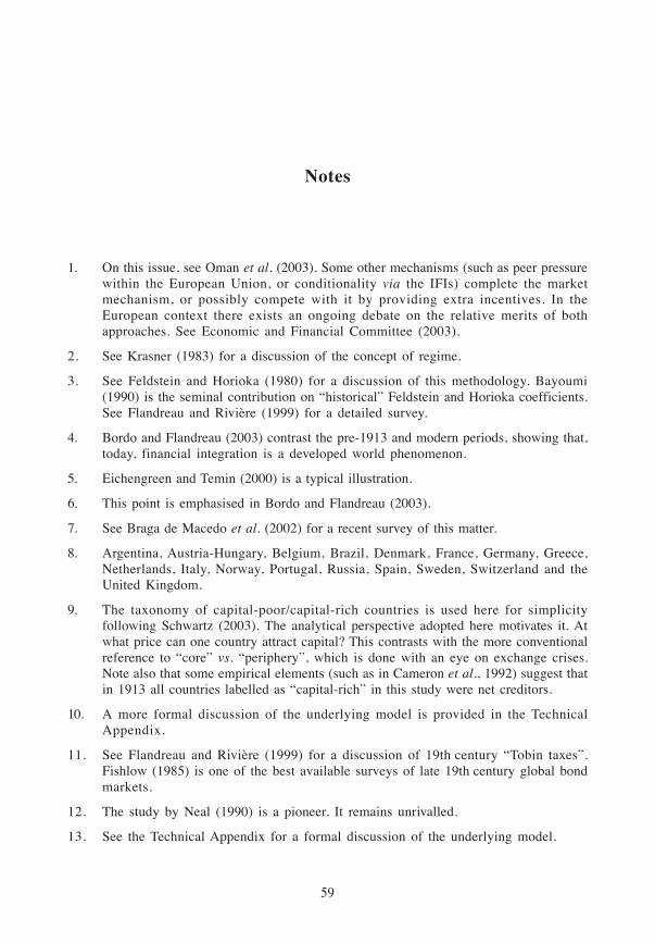
59

Notes

1. On this issue, see Oman et al. (2003). Some other mechanisms (such as peer pressurewithin the European Union, or conditionality via the IFIs) complete the marketmechanism, or possibly compete with it by providing extra incentives. In theEuropean context there exists an ongoing debate on the relative merits of bothapproaches. See Economic and Financial Committee (2003).

2. See Krasner (1983) for a discussion of the concept of regime.

3. See Feldstein and Horioka (1980) for a discussion of this methodology. Bayoumi(1990) is the seminal contribution on “historical” Feldstein and Horioka coefficients.See Flandreau and Rivière (1999) for a detailed survey.

4. Bordo and Flandreau (2003) contrast the pre-1913 and modern periods, showing that,today, financial integration is a developed world phenomenon.

5. Eichengreen and Temin (2000) is a typical illustration.

6. This point is emphasised in Bordo and Flandreau (2003).

7. See Braga de Macedo et al. (2002) for a recent survey of this matter.

8. Argentina, Austria-Hungary, Belgium, Brazil, Denmark, France, Germany, Greece,Netherlands, Italy, Norway, Portugal, Russia, Spain, Sweden, Switzerland and theUnited Kingdom.

9. The taxonomy of capital-poor/capital-rich countries is used here for simplicityfollowing Schwartz (2003). The analytical perspective adopted here motivates it. Atwhat price can one country attract capital? This contrasts with the more conventionalreference to “core” vs. “periphery”, which is done with an eye on exchange crises.Note also that some empirical elements (such as in Cameron et al., 1992) suggest thatin 1913 all countries labelled as “capital-rich” in this study were net creditors.

10. A more formal discussion of the underlying model is provided in the TechnicalAppendix.

11. See Flandreau and Rivière (1999) for a discussion of 19th century “Tobin taxes”.Fishlow (1985) is one of the best available surveys of late 19th century global bondmarkets.

12. The study by Neal (1990) is a pioneer. It remains unrivalled.

13. See the Technical Appendix for a formal discussion of the underlying model.

60

14. The EMBI is just the average yield premium on capital-poor countries for a givenyear. Alternative weighting techniques do not change the basic message.

15. Bayoumi (1990) must be credited for having been the first to point out that financialintegration is not the result only of formal capital controls. He referred to thepossibility of “endogenous behaviour” acting as a barrier to international financialintegration.

16. For recent discussions of the question of interest-rate convergence see Foreman-Peck (1983). This pattern is also discussed in Eichengreen (1996), Flandreau et al.(1998) and McKinnon (1996).

17. Interest rates are constructed using securities listed in the Paris or London stockmarkets. Sources used are Le Rentier and The Economist. Arbitrage ensured that forany security quoted in both markets differences were negligible. Uruguay, Mexicoand Chile were added to the complete list of countries provided in the Appendix.

18. See Cairncross (1953) for a discussion of British foreign lending. Ford (1962) discussesthe ebbs and flows of capital between Britain and Argentina. For a discussion of thewelfare gains/costs of foreign lending, see McCloskey (1970).

19. See also Eichengreen (1992) for arguments along similar lines. An early version ofthis view was the thesis of the “declining morality” of the market place, whichdeveloped after 1900. At that date, some observers deplored that markets werebecoming insufficiently discriminating. This thesis was developed by former leadersof underwriting syndicates, such as the Rothschilds, who saw their market power inunderwriting erode as competition grew. In their eyes, borrowers got better termsonly because of intensified pressure among lenders (Ferguson, 1998).

20. See Eichengreen and Flandreau (1997) for a historical account and review ofarguments. Early sceptics of the virtues and reality of the gold standard includeNogaro (1940) and Triffin (1964).

21. This notion may be found at the heart of recent discussions of pre-1914 financialglobalisation, such as Eichengreen (1997), McKinnon (1996), Bordo and Rockoff(1996), Obstfeld and Taylor (2003a, 2003b) and Clemens and Williamson (2002). Ifproduct differentiation has led various authors to stress various aspects of theprocess, a basic consensus can nonetheless be identified. It is this consensus that isreviewed here.

22. This view was pioneered by Bordo and Rockoff (1996).

23. As a matter of fact, so strong is the notion that global economic integration beforeWWI had everything to do with gold adherence that the use of gold dummies tocapture greater integration is turning into an industry. See Estevadeordal et al. (2003)and Lopez-Cordova and Meissner (2000) for examples of the use of gold dummies inthe context of international trade.

24. See Obstfeld and Taylor (2003a), who consider a broader range of possible variablesthan Bordo and Rockoff do and report depressingly negative results beyond theeffect of gold. Since they explain this in reference to a possible endogeneity problemwith gold adherence capturing all the information from the other variables, they canbe seen as basically siding with Bordo and Rockoff (1996).

61

25. Here, for simplicity, floating is considered as the only alternative to gold adherenceduring 1880-1913. There were some countries that operated convertible silverstandards (such as India), but with the end of bimetallism in 1873, silver adherenceessentially amounted to a free float (see Eichengreen and Flandreau, 1996, andFlandreau, 2003a).

26. Technically, the model uses as a left-hand variable the premium a given country hadto pay above Britain’s interest rates in a given year. The right-hand variable is anindex variable reflecting whether or not the country was on gold during that year.Country-specific controls are also included. The results of this regression can befound in the Technical Appendix. Because no other variable is included, one can besure of obtaining estimates that, if anything, exaggerate the effect of gold adherence.Recall that the other macroeconomic variables considered by Bordo and Rockoff(1996) and Obstfeld and Taylor (2003a) turned out to be non-significant.

27. See Reis (1996) and Braga de Macedo et al. (2001) for a discussion of the Portugueseexperience. See Martin Aceña (2000) for a discussion of the Spanish one. Chile couldbe added to the list of the non-gold, yet convergent countries.

28. On Russia’s “cosmetism”, see Conant (1896).

29. On Japan’s development policies, see Rosovsky (1961). On its external borrowing,see Suzuki (1994).

30. As was sometimes the case, the adoption of the gold standard was accompanied bya debt conversion. The implication is a repurchase of outstanding obligations at parand their reissue at a lower price. This means that standard estimates of the yieldsthat rely on the classic coupon/price formula are biased.

31. It might also be added that the adoption of the gold standard was truly part of abroad international public relations operation. Not incidentally, Count MatsukataMasayoshi’s famous Report on the Adoption of the Gold Standard (1899) was writtenin English. There is a danger that modern economists may become the last victimsof late 19th century PR campaigns. On the symbolic role of gold adherence for19th century developers, see Gallarotti (1995).

32. Weber (1904) argued that the Protestant ethic was more favourable to development.

33. Baxter (1871), pp. 125-126.

34. Bamberger, Deutsche Rundschau, October 1877, quoted by Cernuschi (1878), Ladiplomatie monétaire en 1878, p. 90. Bamberger was a prominent German politicianand authorised writer, whose role in the unification of Germany and subsequentadoption of the gold standard was paramount. He was a leader of the Liberal partywhose goals conflicted with Bismarck’s objectives of centralisation. See Koehler(1999).

35. “Millennium Resolution: No more funny money”, Financial Times,3rd January 2000.

36. Leroy-Beaulieu (1899), Tome II, p. 629. Leroy-Beaulieu was the editor of the Frenchcounterpart to The Economist, L’Economiste Français.

37. James de Rothschild, 2nd June 1868, Quoted in Gille (1967).

62

38. Laffitte (1824), pp. 41-42. For similar views coming from the other side of the Channel,see Ferguson (1998).

39. Flandreau (2003d). This research was a source of inspiration for the work of Tomz(2001), to whom the authors communicated some of their data. On the history ofCrédit Lyonnais, see Bouvier (1961).

40. See Flandreau (2003d) for data on the budget and number of employees of the researchdepartment.

41. Since we know to what group each country belonged and the intermediate variablescontemporaries monitored, we can assess the weight that each variable had on theranking.

42. Some discrepancies are to be expected, because these ratings, which the Lyonnaiskept secret and used to advise its clientele of depositors, were meant to signal someinvestment opportunities that had been underestimated by the market.

43. We only have one instance of formal rating, while there is ample suggestion thatsuch exercises were routinely carried out.

44. For instance, the third group comprised in 1898 mostly countries that were, hadrecently been or were about to be in default. While this motivated a general gradingto “junk” status by Lyonnais economists (explaining the virtually vertical axis inwhich we find Portugal, Greece, Brazil, Argentina and Serbia) the market nonethelessdiscriminated among junk countries depending on default settlement prospects.This motivated potentially very different yield premiums, although the ratingprocedure tended to downplay idiosyncrasies among defaulters.

45. Correlation coefficients are 0.82 for spread vs. grade and 0.84 for log spread vs.grade.

46. The authors’ understanding from actual reading of other sources is that individualanalyses such as Lyonnais’ were widely shared by the market.

47. Cliometrics was pioneered by Nobel Prize winners Robert Fogel and Douglas North,among others.

48. Formally, Rit-Rukt = αι+βXt+ωt. A refinement of the model is the use of the capital assetpricing formula (CAPM). Bordo and Rockoff (1996) and Mauro et al. (2002) employ it.Note that from the point of view of the “theories in use”, it is safer to stick to the mostparsimonious model and not complicate matters by relying on later theoreticaldevelopments, such as the CAPM.

49. Flandreau et al. (1998) pioneered the “structuralist” view, which holds thatmacroeconomic variables were strongly correlated with bond spreads. Ferguson andBatley (2001) developed a “political” view according to which political events werethe drivers of spreads in the 19th century.

50. Obstfeld and Taylor (2003a) and (2003b) are prototypes.

51. Consider the situations of Japan and Argentina around 2000. While the debt burdenof Japan was around 125 per cent of GDP, Argentina’s stood at about 45 per cent;and yet a crisis occurred in Argentina. The reason is that no debt burden can be

63

properly assessed if one does not take into account the corresponding “annuity”.Japan borrows at cheap rates while Argentina faced huge premiums. The result isthat the actual burden supported by Argentina (10 per cent of GDP) was much largerthan that supported by Japan (4.3 per cent). In the end, Argentina turned out to bethe more vulnerable country. (Sources: OECD, 2002 and Moody’s InvestorsService, 2002).

52. That is how their significance is interpreted in Flandreau et al. (1998). In a similar vein,the historical GDP numbers were literally not available to contemporaries, becausethey typically are later reconstructions. They are nonetheless correlated with variablesthat were available to contemporaries.

53. Leroy-Beaulieu (1878), Vol. 2, Chapter XIV, “Des moyens d’évaluer le poids des dettespubliques.”

54. This is because contemporaries sought to capitalise income flows (e.g. income fromland) in order to reach an evaluation of the value of the corresponding assets.

55. This despite Mulhall’s pioneering work. In effect, Mulhall’s optimistic numbers forArgentina (Mulhall, 1887) were held responsible for fuelling excessive enthusiasm.The publications of the Société Internationale de Statistique contain earlycontributions to the modern art of GDP estimation.

56. Leroy-Beaulieu (1878), Vol. 2, p. 575. A similar caution is visible among Lyonnaiseconomists (see Flandreau, 2003d).

57. Baxter (1871), p. 8 and various issues of the Bulletin de la Société Internationale deStatistique.

58. Baxter (1871), Théry (1887), Haupt (1894) and Canovai (1898) are characteristicexamples.

59. Leroy-Beaulieu (1878), p. 578. A similar view prevailed in Crédit Lyonnais studiesand in many other places. See Flandreau (2003d).

60. In a famous study of England in the 18th and 19th centuries, Barro (1987) found astatistically significant link between deficits and interest rates. During the periodunder study, however, deficits were motivated mostly by wars and thus surroundedby much uncertainty. If current deficits signal future ones, their effect on riskpremiums can be substantial, because agents discount the consequences of increasedindebtedness.

61. So that their influence on ratings seems to have been heavily discounted, whicheconometric investigations of Lyonnais ratings confirmed. For a study of the“monetary files” at Crédit Lyonnais, see Flandreau (2003b).

62. For instance, in the standardised country scorecards it produced, the Crédit Lyonnaishad a special entry for the “monetary regime”, but upon closer inspection it appearsthat it is the legal (nominal) regime which was recorded there, and not the actual one!

63. The analogy between this way of reasoning and the so-called tax based theory ofmoney is striking. Its empirical success, when used on 19th century data(Calomiris, 1988), may be understood in this respect.

64

64. In effect, both the Lyonnais and Fenn’s Compendium suggested that inconvertiblepaper money be added to the debt burden as a virtual liability. A table provided bythe 1889 edition of Fenn’s Compendium has an asterisk (p. xv) for Austria-Hungary,Italy, Russia, Argentina and Brazil that reads, “depreciated paper currency estimatedto entail a 5 per cent burden on these countries.” This is evidence of the debt-burdensignificance of monetary variables.

65. For contemporaries’ views on the irrelevance of the cover ratio, see Flandreau (2003b).

66. This result was rediscovered more recently. It is known as the Tanzi effect(Tanzi, 1989, 1990).

67. Leroy-Beaulieu (1878) 2nd ed., Vol. II, p. 579-80. Similarly, the reports on public financesin the Statesman’s Yearbook were careful to distinguish between domestic and foreignliabilities. In the Lyonnais archives, we find ample evidence that economists workedhard to sort out the contribution of exchange-rate variations to changes in the burdenof the public debt. For this purpose, they tried to isolate the domestic and externaldebts, and used this information to assess the change in interest service that wouldresult from a given depreciation of the exchange rate.

68. This way one finds applied economists trying to assess the fiscal implications of the1898 military conflict between Spain and the United States. Their conclusion wasthat the financial imbalance between the two countries suggested that the war wouldbe short or the Spaniards crazy. This led The Economist rightly to forecast a shortconflict. Crédit Lyonnais Archives DEEF 82505.

69. The Economist complained in 1873 that such a procedure could involve seriousdangers if it were to become a routine.

70. North and Weingast (1989). See also the 2000 special issue of the Journal of EconomicHistory. For a contrary view, see O’Brien (2001).

71. Leroy-Beaulieu (1899), p. 630 (6th ed. of Sciences des Finances). The first two editionsdid not include the qualification on “discipline”. Leroy-Beaulieu explains that headded it because the French experience suggested to him that “un certain régimeparlementaire brouillon et subversif est une cause de gaspillage effréné.” (Id. p. 630).

72. For a reprint of Russia’s political risk analysis, see Crédit Lyonnais (1998), PolitiqueEtrangère.

73. The exports-to-reserves ratio was also tried, as suggested by some comments in theLyonnais archives. The results are reported in the Technical Appendix.

74. While cross-sectional measures of trade openness can rely on trade per head, in agiven currency unit at a given point in time, panel comparisons require using abenchmark that controls for prices. Contemporaries did not construct uniform priceindices, however. This study thus normalised the ratio of exports per head of countryi at date t by dividing it by the British ratio of exports per head at date t. Technically,

[Exports(i,t)/population(i,t)]/[Exports(UK,t)/population(UK,t)]

75. The table reports the effect of a 0.1 per cent average monthly depreciation over oneyear, i.e. a 1.2 per cent average depreciation over the year.

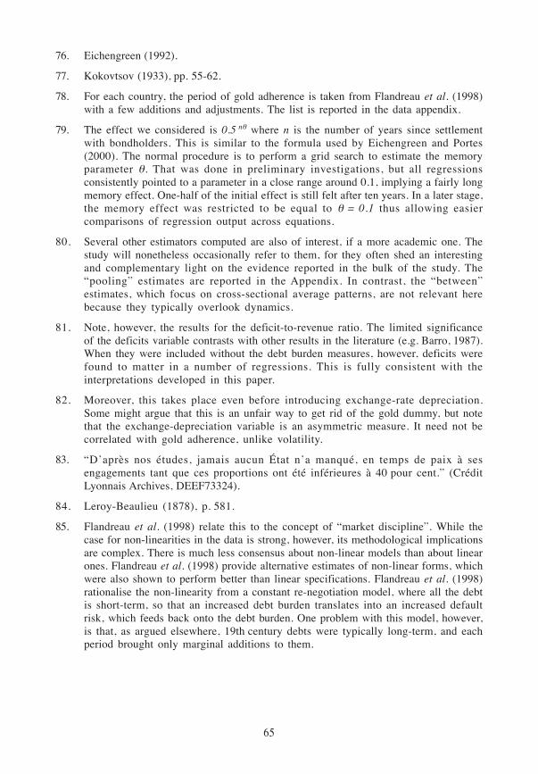
65

76. Eichengreen (1992).

77. Kokovtsov (1933), pp. 55-62.

78. For each country, the period of gold adherence is taken from Flandreau et al. (1998)with a few additions and adjustments. The list is reported in the data appendix.

79. The effect we considered is 0.5 nθ where n is the number of years since settlementwith bondholders. This is similar to the formula used by Eichengreen and Portes(2000). The normal procedure is to perform a grid search to estimate the memoryparameter θ. That was done in preliminary investigations, but all regressionsconsistently pointed to a parameter in a close range around 0.1, implying a fairly longmemory effect. One-half of the initial effect is still felt after ten years. In a later stage,the memory effect was restricted to be equal to θ = 0.1 thus allowing easiercomparisons of regression output across equations.

80. Several other estimators computed are also of interest, if a more academic one. Thestudy will nonetheless occasionally refer to them, for they often shed an interestingand complementary light on the evidence reported in the bulk of the study. The“pooling” estimates are reported in the Appendix. In contrast, the “between”estimates, which focus on cross-sectional average patterns, are not relevant herebecause they typically overlook dynamics.

81. Note, however, the results for the deficit-to-revenue ratio. The limited significanceof the deficits variable contrasts with other results in the literature (e.g. Barro, 1987).When they were included without the debt burden measures, however, deficits werefound to matter in a number of regressions. This is fully consistent with theinterpretations developed in this paper.

82. Moreover, this takes place even before introducing exchange-rate depreciation.Some might argue that this is an unfair way to get rid of the gold dummy, but notethat the exchange-depreciation variable is an asymmetric measure. It need not becorrelated with gold adherence, unlike volatility.

83. “D’après nos études, jamais aucun État n’a manqué, en temps de paix à sesengagements tant que ces proportions ont été inférieures à 40 pour cent.” (CréditLyonnais Archives, DEEF73324).

84. Leroy-Beaulieu (1878), p. 581.

85. Flandreau et al. (1998) relate this to the concept of “market discipline”. While thecase for non-linearities in the data is strong, however, its methodological implicationsare complex. There is much less consensus about non-linear models than about linearones. Flandreau et al. (1998) provide alternative estimates of non-linear forms, whichwere also shown to perform better than linear specifications. Flandreau et al. (1998)rationalise the non-linearity from a constant re-negotiation model, where all the debtis short-term, so that an increased debt burden translates into an increased defaultrisk, which feeds back onto the debt burden. One problem with this model, however,is that, as argued elsewhere, 19th century debts were typically long-term, and eachperiod brought only marginal additions to them.

66

86. Consider two perpetual bonds, both gold denominated. The risk free bond (UK’sbond) pays coupon 5 and trades at Puk. The risky bond (country i’s bond) payscoupon 5 and trades at Pi. For a risk neutral investor, we must have Pi=Puk(1-πi)+0.πi where πi is a measure of the probability of a future default; yields arerespectively defined as Ruk = 5/Puk and Ri= 5/Pi. We therefore have 5=Ruk.Puk=Ri.Pi.This finally gives πi =(Ri-Ruk)/Ri.

87. This is reminiscent of the recent literature on exchange-rate behaviour and politicalregimes. See Freeman et al. (1999). See Appendix for individual parameter estimates.

88. For a pioneering formulation of this hypothesis, see Eichengreen (1992).

89. Countries initially on the verge of crisis with very high burdens tend to have thehighest interest premiums. They are the ones for which the convergence and debtreduction are most striking.

90. Recall that if B is the debt burden, we have B=S/Tax, where S is the interest serviceand Tax the tax revenue. Neglecting the role of exchange-rate changes, this can berewritten as B=S/(Y.T.P) where Y is real income, T is the tax rate, and P the price level.Finally, ΔB/B=ΔS/S-[ΔY/Y+ΔT/T+ΔP/P], where the growth rate, the change in thetax rate and inflation are recognised.

91. For simplicity (i.e. to keep the chart legible) the contributions of default andexchange-rate depreciation are omitted.

92. Flandreau et al. (1998) show that deficits accumulated at a higher rate after 1900 thanbefore.

93. Gold adherence implies that the money supply is set exogenously by gold discoveries.The price level then becomes endogenous (see Barro, 1983). Note that thecontribution of inflation to the decline of debt burdens was large, as emphasised byFlandreau et al. (1998).

94. “Introduction”, Fenn’s Compendium, 1889 edition, pp. xix and xx. Capitalising at 5 percent means that a service of 5 is tantamount to a debt of 100. If exports stand at 25,then the debt to exports ratio stands at 4. Converting Fenn’s Compendium’s debt toexports danger threshold of 4 in (more conventional) terms of interest service toexports, we get that the interest service cannot exceed 5/25=20 per cent of annualexports as indicated in the text.

95. See Irwin (1996) for a stimulating intellectual survey.

96. On the interactions between trade expansion and bullion discoveries, see Flandreau(2003a).

97. Bairoch (1993) places the expansion of European trade at about 5-6 per cent.European economies grew at 1-2 per cent.

98. The emphasis on Europe is important here. As Bairoch (1993) argued, free traderemained a distinctly Western European phenomenon in the 19th century.

99. See Jenks (1927) for British capital exports and Cameron (1961) for French capital exports.

100. See Cameron (1961). Flandreau (2000) shows the association between trade treaties,monetary arrangements and financial interdependencies.

67

101. On the role of opinions in the mid-19th century free-trade epidemic, see Kindleberger(1988).

102. Gerschenkron (1962). This is the so-called “relative backwardness thesis”.

103. In other words, even a loss-making railway, provided that it did not cost more to runthan it brought in income, reduced the net service of the corresponding debt. Consider,for instance, a railway loan that involves an annual coupon payment of R, railway-operating costs of C and railway income of I. Provided that I>C, part of the debtburden is offset.

104. Nineteenth-century observers were only rediscovering things that had been at theheart of early experiences of economic development, beginning with Britain. AsBrewer (1990) and O’Brien (2001) emphasised, the beginnings of the IndustrialRevolution in Britain in the 18th century had been tightly associated with deeptransformations of the fiscal machinery. The creation of a comparatively efficienttax bureaucracy enabled successive British governments to rely on abundantresources that in turn permitted both extensive borrowing and the building of areputation for strong willingness to pay back creditors.

105. See Flandreau (2003d) for a discussion. Mulhall (1896) and Fenn’s Compendium (1889),among others, are early illustrations. In a recent paper Kelly (1998) reports evidencethat the composition of public debts did matter in determining market access.

106. On these difficulties, see Fenn’s Compendium (1889), pp. xvi-xvii. “The question thenarises: To what extent are these [public debt burdens] covered by reproductive works?Taking the heaviest debt per head on the entire list — that of Queensland — we findthat it has been raised to the extent of some £15 000 000 for railways, £750 000 fortelegraphs, £1 500 000 for harbours and navigations, £800 000 for roads and bridges,and £1 000 000 for loans to municipalities … for local water supply and other works,or together £19 000 000 out of a total of £25 000 000 bonds issued; and if to theseitems were added the money absorbed by immigration expenses and public buildings,we should find practically the whole of the debt had been contracted for works ofutility, even if some of them are not directly reproductive. … We are scarcely, however,entitled to write off blindfold the whole of this outlay upon public works. … It hasbeen impossible … to deal with accounts of all countries … and in the Table of netIndebtedness [which we give below showing the true burden of public debts] theremay in some cases be assets which have not been fully allowed for.”

107. It is no surprise, therefore, that Crédit Lyonnais economists sought to develop asystematic way to sort out “true” government revenues from gross numbers. As aresult, the measure of the debt burden, which they monitored, subtracted from theinterest service the net income from public companies. This in turn enabled them toassess the value of government assets. The next stage, of course, was to make pair-wise comparisons of the efficiency of alternative governments.

108. As reported by Lyonnais economists, the Austrian state railways were known to bemuch more profitable than their Hungarian counterparts. This shows that it is notenough to know the purpose of a given public project in order to assess its quality.

68

109. The chronological boundaries are obviously somewhat arbitrary. While the Baringcrisis is emphasised here as a watershed, other timings could be considered. Inparticular, 1873-89 is clearly a period during which both criteria were used incombination.

110. If trade and taxation are constant fractions of national income, they should display afixed proportion for each given country across time and thus give very similar resultswhen fixed effects are introduced in the regression. Moreover, if as suggested byRodrik (1998) there is a tight positive association between government size (taxrevenues as a share of GDP) and openness (trade as a share of GDP) then the twovariables should be perfect substitutes in all regressions. Note that the empiricalsample used here did not uncover the relation discussed by Rodrik.

111. Strictly speaking, the trade test performed here uses the annuity on the public debt(interest service), not the capitalisation of this annuity at a uniform rate of 5 per centas suggested by Fenn’s Compendium. It is clear, however, that the two measures areessentially substitutes.

112. This is the last pre-crisis year for which Fenn’s Compendium provides figures for thetrade test.

113. Note that Spain, which was the most recent experience of default in the 1880s,displayed when it collapsed a tax test of about 0.47 (comparable to Portugal in1888) but a trade test standing at 25 (Fenn’s Compendium, 1889, p. xvii). In thatcase, the trade test rang the emergency signal.

114. This conclusion may help to reconcile recent seemingly conflicting conclusions inthe literature. While Triner (2001) argues that contagion spread from Argentina toBrazil, Mauro et al. (2002) maintain there was none. They reach this conclusion byemphasising that investors of the time were able to focus on “fundamentals”. Thisclaim conflicts with contemporary accounts, which stressed the “reverberation” ofthe Argentine crisis (see Conant, 1896, and Flandreau, 2003c). On the other hand, theword “reverberation” suggests that the transmission of the crisis went through theperceptions of the money centre (see Calvo, 1999, for a discussion of the potentialrole of money centres in transmitting financial instability). The analysis in this studysuggests that if a crisis leads to some re-scaling of the “fundamentals”, then theconclusion of Mauro et al. (2002) need not be taken as evidence against “contagion”.

115. This conclusion fits squarely with the findings of a vast literature that has documentedboth the effect of recent financial crises on ratings and the reverse impact of ratingson crises. See, for example, Cantor and Packer (1996), Eichengreen and Mody (1998),Kamin and von Kleist (1999), Reinhart (2002), Kräussl (1999) and Reisen and vonMaltzan (1999).

116. This obviously contrasts with the logic of financial integration as it has been achievedhistorically in national contexts. There, institutions and financial technology havebeen shown to play an essential role. See, for example, Davis (1980).

117. See, for example, O’Rourke and Williamson (1999) and Clemens and Williamson (2002)for characteristic illustrations.

69

118. For the conventional view, see Bordo and Rockoff (1996), Sussman and Yafeh (1999),Obstfeld and Taylor (2003a, 2003b) and Eichengreen et al. (2003).

119. This finding was emphasised by Bordo and Flandreau (2003).

120. On the so-called “original sin”, see Eichengreen et al. (2003). On its historical aspects,see Flandreau and Sussman (2003).

121. This occurred quite apart from formal procedures whereby bondholders formallyprevented defaulting governments from getting access to capital markets(Flandreau, 2003c).

122. These conclusions clearly contrast with the conventional emphasis (see, for example,O’Rourke and Williamson, 1999) on trade openness as the main source of pre-1914convergence. This monograph has shown that pre-1914 financial convergence hadorigins much different from what has been argued so far.

71

Technical Appendix

The Background Model

Consider one capital-poor country i, defining as “capital-poor” a nation that hasa large growth potential and thus needs to accumulate capital. In view of consumptionsmoothing, capital accumulation is better done via capital imports than through domesticsaving. In other words, this country has savings Si,0 that typically fall short of investmentneeds. It also has a demand schedule for capital, D(i), that is a decreasing function ofthe yield premium ri-ruk. (The yield premium is measured here as the interest ratedifferential with the capital-rich country — for simplicity, the United Kingdom).Country i faces a supply of funds S(i, G0) which increases with ri-ruk. The importantpoint is that S shifts with changes of parameter G0, which represents the risk of lendingto country i. This risk is determined by market perceptions of the quality of thepolicies that country i follows.

Now look first at the left-hand side of Figure A.1. Thanks to the foreign capitalinflow, domestic investment equals Ii,0, and the current account deficit, CC (i.e. thenet capital inflow) equals Ii,0 - Si,0, where Si.0 is domestic saving. Domestic shocks ondomestic saving will have no impact on domestic investment, because any fall insaving will be offset by capital inflows. As a result, there will be no correlationbetween Ii,0 and Si,0. Suppose now that perceptions of the risk of lending to country iincrease from G0 to G1. As the right-hand side of the figure depicts, the capital supplyschedule shifts to the left as foreign investors become more reluctant to invest incountry i. As the equilibrium yield premium rises, the supply of foreign capitalevaporates. There is a level of risk where the country becomes deprived of foreigncapital. In the example shown, the increase in risk forces the current account intobalance and shuts down capital inflows, so that Ii,1 = Si,1. If the perceived risk is largerthan G1, the correlation between domestic savings and investment will be perfect (equalto one), and the Feldstein-Horioka coefficients will point to a situation of financial“dis-integration”. Therefore, the analysis predicts that there should be a relation betweenintegration coefficients and risk premiums. This explains Figure 1 in the text.

72

r - ri uk

r - r

r - r

i1 uk

i0 uk

S(δ )0

D

S I = S + CCi0 i0 i0

S(δ )0

S(δ )1

D

S = Ii1 i1

Figure A.1. Financial Openness and the Yield Premium

Detailed Results: Alternative Specifications

The text reported summary results for the most complete model, with all effectsincluded. The tables below show outcomes for both the interest-spread model and thedefault probability model with more limited combinations of the explanatory variables.They highlight the decline in explanatory power of the gold-adherence dummy asmore variables enter and especially the impact of taking crises into account. (Notethat since the capital-rich countries were always on gold one cannot include a golddummy for them.) They also accent the effect of the political crisis variables on theeffect and significance of exchange depreciation. Finally, while not always significant,the trade-openness variable works in different ways for different groups of countries.Openness seems to be good for capital-rich countries, but less so for capital-poorones. This makes much sense in view of the discussion in Section IX.

73

Table A.1. Fixed Effects, All Countries, 1880-1913 Interest-Rate Spread Model

1 2 3 4 5

1. Structural factors: - Interest service/Revenue - 8.849 (10.91) 8.665 (9.99) 8.715 (9.73) 7.751 (8.50) - Reserves/Banknotes - - - 0.414 (-1.41) -0.286 (-0.96) - Exports/Population - - - 0.782 (2.02) 0.601 (1.59) - Deficit/Revenue - - - 0.710 (3.08) 0.725 (3.16) - Exch.-rate volatility - - - 2.208 (2.76) 0.997 (1.14) 2. Reputation factors: - Default - 4.994 (22.31) 4.999 (21.91) 5.010 (22.24) 4.836 (21.66) - Memory - 0.882 (3.32) 0.849 (3.12) 0.893 (3.26) 0.703 (2.56) 3. Political variables: - Franchise - - -0.827 (-0.66) -2.424 (-1.71) -2.427 (-1.77) - Political crises - - - - F=3.797 (*) 4. Gold -1.546 (-7.03) - -0.034 (-0.25) 0.280 (1.57) 0.056 (0.32) SBIC 927.991 669.375 675.286 675.383 696.069 Log L. -875.514 -610.724 -610.461 -598.210 -563.332 Adjusted R2 0.493 0.831 0.831 0.838 0.854 Number of observations: 480. Not shown are the country-specific constants. Numbers in parentheses are heteroscedasticity-consistent Student t statistics. Corresponding standard errors are computed from a heteroscedasticity-consistent matrix (Robust-White). In all cases, F-tests choose Fixed Effects over simple pooling. (*) F-test significant at 5 per cent. The Schwartz Bayesian Information Criteria (SBIC) is a model selection test, which has the asymptotic property of picking up the true model, if the true model is one of the alternatives being tested.

Table A.2. Fixed Effects, Capital-Rich Countries, 1880-1913 Interest-Rate Spread Model

1 2 3 4 5

1.Structural factors: - Interest service/Revenue - 5.200 (8.61) 4.231 (6.61) 3.885 (5.61) 4.144 (6.18) - Reserves/Banknotes - - - 0.182 (1.05) 0.223 (1.34) - Exports/Population - - - -0.131 (-1.12) -0.160 (-1.41) - Deficit/Revenue - - - 0.248 (1.29) 0.319 (1.71) - Exch.-rate volatility - - - 2.502 (1.69) 2.825 (1.97) 2.Reputation factors: - Default - - - - - - Memory - - - - - 3.Political variables: - Franchise - - -1.305 (-3.79) -0.916 (-2.29) -0.839 (-2.17) - Political crises - - - - F=4.15 (*) 4. Gold - - - - - SBIC - -2.37208 -6.91986 0.243620 -5.92347 Log L. - 26.8041 34.0666 37.7618 46.6436 Adjusted R2 - 0.520 0.547 0.554 0.585 Number of observations: 228. Not shown are the country-specific constants. Numbers in parentheses are heteroscedasticity-consistent Student t statistics. Corresponding standard errors are computed from a heteroscedasticity-consistent matrix (Robust-White). In all cases, F-tests choose Fixed Effects over simple pooling. (*) F-test significant at 5 per cent. Here the F-Test coincides with a T-test. The Boer War was the only common factor.

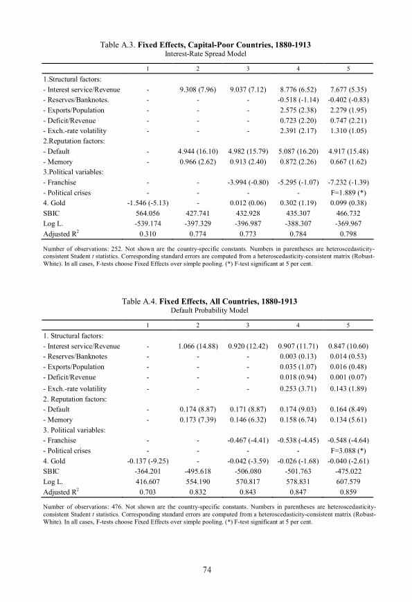
74

Table A.3. Fixed Effects, Capital-Poor Countries, 1880-1913 Interest-Rate Spread Model

1 2 3 4 5

1.Structural factors: - Interest service/Revenue - 9.308 (7.96) 9.037 (7.12) 8.776 (6.52) 7.677 (5.35) - Reserves/Banknotes. - - - -0.518 (-1.14) -0.402 (-0.83) - Exports/Population - - - 2.575 (2.38) 2.279 (1.95) - Deficit/Revenue - - - 0.723 (2.20) 0.747 (2.21) - Exch.-rate volatility - - - 2.391 (2.17) 1.310 (1.05) 2.Reputation factors: - Default - 4.944 (16.10) 4.982 (15.79) 5.087 (16.20) 4.917 (15.48) - Memory - 0.966 (2.62) 0.913 (2.40) 0.872 (2.26) 0.667 (1.62) 3.Political variables: - Franchise - - -3.994 (-0.80) -5.295 (-1.07) -7.232 (-1.39) - Political crises - - - - F=1.889 (*) 4. Gold -1.546 (-5.13) - 0.012 (0.06) 0.302 (1.19) 0.099 (0.38) SBIC 564.056 427.741 432.928 435.307 466.732 Log L. -539.174 -397.329 -396.987 -388.307 -369.967 Adjusted R2 0.310 0.774 0.773 0.784 0.798 Number of observations: 252. Not shown are the country-specific constants. Numbers in parentheses are heteroscedasticity-consistent Student t statistics. Corresponding standard errors are computed from a heteroscedasticity-consistent matrix (Robust-White). In all cases, F-tests choose Fixed Effects over simple pooling. (*) F-test significant at 5 per cent.

Table A.4. Fixed Effects, All Countries, 1880-1913 Default Probability Model

1 2 3 4 5

1. Structural factors: - Interest service/Revenue - 1.066 (14.88) 0.920 (12.42) 0.907 (11.71) 0.847 (10.60) - Reserves/Banknotes - - - 0.003 (0.13) 0.014 (0.53) - Exports/Population - - - 0.035 (1.07) 0.016 (0.48) - Deficit/Revenue - - - 0.018 (0.94) 0.001 (0.07) - Exch.-rate volatility - - - 0.253 (3.71) 0.143 (1.89) 2. Reputation factors: - Default - 0.174 (8.87) 0.171 (8.87) 0.174 (9.03) 0.164 (8.49) - Memory - 0.173 (7.39) 0.146 (6.32) 0.158 (6.74) 0.134 (5.61) 3. Political variables: - Franchise - - -0.467 (-4.41) -0.538 (-4.45) -0.548 (-4.64) - Political crises - - - - F=3.088 (*) 4. Gold -0.137 (-9.25) - -0.042 (-3.59) -0.026 (-1.68) -0.040 (-2.61) SBIC -364.201 -495.618 -506.080 -501.763 -475.022 Log L. 416.607 554.190 570.817 578.831 607.579 Adjusted R2 0.703 0.832 0.843 0.847 0.859 Number of observations: 476. Not shown are the country-specific constants. Numbers in parentheses are heteroscedasticity-consistent Student t statistics. Corresponding standard errors are computed from a heteroscedasticity-consistent matrix (Robust-White). In all cases, F-tests choose Fixed Effects over simple pooling. (*) F-test significant at 5 per cent.

75

Table A.5. Fixed Effects, Capital-Rich Countries, 1880-1913 Default Probability Model

1 2 3 4 5

1. Structural factors: - Interest service/Revenue - 1.238 (6.63) 0.866 (4.37) 0.756 (3.51) 0.889 (4.31) - Reserves/Banknotes - - - 0.068 (1.42) 0.080 (1.76) - Exports/Population - - - -0.025 (-0.76) -0.032 (-1.02) - Deficit/Revenue - - - 0.071 (1.34) 0.095 (1.86) - Exch.-rate volatility - - - 0.708 (1.71) 0.801 (2.04) 2. Reputation factors: - Default - - - - - - Memory - - - - - 3. Political variables: - Franchise - -0.425 (-4.39) -0.330 (-2.97) -0.302 (-2.85) - Political crises - - - - F=4.83 (*) 4. Gold - - - - - SBIC - -286.809 -293.755 -286.948 -296.099 Log L. - 311.162 320.813 324.830 336.686 Adjusted R2 - 0.423 0.468 0.477 0.527 Number of observations: 224. Not shown are the country-specific constants. Numbers in parentheses are heteroscedasticity-consistent Student t statistics. Corresponding standard errors are computed from a heteroscedasticity-consistent matrix (Robust-White). In all cases, F-tests choose Fixed Effects over simple pooling. (*) F-test significant at 5 per cent. Here the F-test coincides with a T-test. The Boer War was the only common factor.

Table A.6. Fixed Effects, Capital-Poor Countries, 1880-1913 Default Probability Model

1 2 3 4 5

1. Structural factors: - Interest service/Revenue - 1.048 (12.10) 0.906 (9.95) 0.851 (8.79) 0.741 (7.19) - Reserves/Banknotes - - - -0.021 (-0.63) -0.021 (-0.60) - Exports/Population - - - 0.156 (2.00) 0.134 (1.60) - Deficit/Revenue - - - 0.009 (0.38) -0.015 (-0.61) - Exch.-rate volatility - - - 0.267 (3.37) 0.163 (1.82) 2. Reputation factors: - Default - 0.176 (7.73) 0.175 (7.71) 0.185 (8.20) 0.178 (7.78) - Memory - 0.169 (6.20) 0.143 (5.24) 0.146 (5.26) 0.110 (3.70) 3. Political variables: - Franchise - - -0.872 (-2.45) -1.030 (-2.91) -1.301 (-3.48) - Political crises - - - - F=1.928 (*) 4. Gold -0.137 (-7.54) - -0.039 (-2.84) -0.018 (-0.97) -0.028 (-1.54) SBIC -144.104 -228.052 -231.013 -227.854 -196.779 Log L. 168.986 258.464 266.954 274.854 293.544 Adjusted R2 0.420 0.712 0.729 0.741 0.758 Number of observations: 252. Not shown are the country-specific constants. Numbers in parentheses are heteroscedasticity-consistent Student t statistics. Corresponding standard errors are computed from a heteroscedasticity-consistent matrix (Robust-White). In all cases, F-tests choose Fixed Effects over versus pooling. (*) F-test significant at 5 per cent.

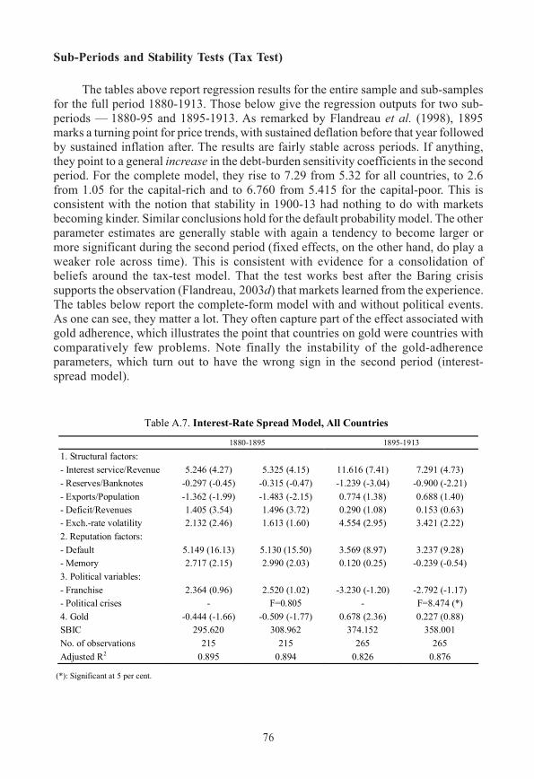
76

Sub-Periods and Stability Tests (Tax Test)

The tables above report regression results for the entire sample and sub-samplesfor the full period 1880-1913. Those below give the regression outputs for two sub-periods — 1880-95 and 1895-1913. As remarked by Flandreau et al. (1998), 1895marks a turning point for price trends, with sustained deflation before that year followedby sustained inflation after. The results are fairly stable across periods. If anything,they point to a general increase in the debt-burden sensitivity coefficients in the secondperiod. For the complete model, they rise to 7.29 from 5.32 for all countries, to 2.6from 1.05 for the capital-rich and to 6.760 from 5.415 for the capital-poor. This isconsistent with the notion that stability in 1900-13 had nothing to do with marketsbecoming kinder. Similar conclusions hold for the default probability model. The otherparameter estimates are generally stable with again a tendency to become larger ormore significant during the second period (fixed effects, on the other hand, do play aweaker role across time). This is consistent with evidence for a consolidation ofbeliefs around the tax-test model. That the test works best after the Baring crisissupports the observation (Flandreau, 2003d) that markets learned from the experience.The tables below report the complete-form model with and without political events.As one can see, they matter a lot. They often capture part of the effect associated withgold adherence, which illustrates the point that countries on gold were countries withcomparatively few problems. Note finally the instability of the gold-adherenceparameters, which turn out to have the wrong sign in the second period (interest-spread model).

Table A.7. Interest-Rate Spread Model, All Countries

1880-1895 1895-1913

1. Structural factors: - Interest service/Revenue 5.246 (4.27) 5.325 (4.15) 11.616 (7.41) 7.291 (4.73) - Reserves/Banknotes -0.297 (-0.45) -0.315 (-0.47) -1.239 (-3.04) -0.900 (-2.21) - Exports/Population -1.362 (-1.99) -1.483 (-2.15) 0.774 (1.38) 0.688 (1.40) - Deficit/Revenues 1.405 (3.54) 1.496 (3.72) 0.290 (1.08) 0.153 (0.63) - Exch.-rate volatility 2.132 (2.46) 1.613 (1.60) 4.554 (2.95) 3.421 (2.22) 2. Reputation factors: - Default 5.149 (16.13) 5.130 (15.50) 3.569 (8.97) 3.237 (9.28) - Memory 2.717 (2.15) 2.990 (2.03) 0.120 (0.25) -0.239 (-0.54) 3. Political variables: - Franchise 2.364 (0.96) 2.520 (1.02) -3.230 (-1.20) -2.792 (-1.17) - Political crises - F=0.805 - F=8.474 (*) 4. Gold -0.444 (-1.66) -0.509 (-1.77) 0.678 (2.36) 0.227 (0.88) SBIC 295.620 308.962 374.152 358.001 No. of observations 215 215 265 265 Adjusted R2 0.895 0.894 0.826 0.876

(*): Significant at 5 per cent.

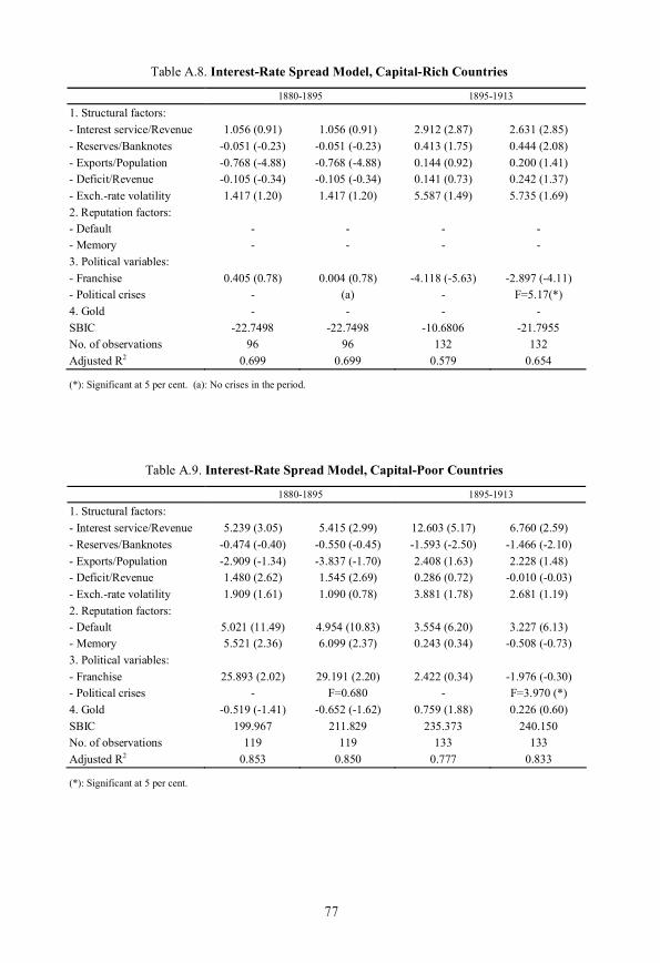
77

Table A.8. Interest-Rate Spread Model, Capital-Rich Countries

1880-1895 1895-1913

1. Structural factors: - Interest service/Revenue 1.056 (0.91) 1.056 (0.91) 2.912 (2.87) 2.631 (2.85) - Reserves/Banknotes -0.051 (-0.23) -0.051 (-0.23) 0.413 (1.75) 0.444 (2.08) - Exports/Population -0.768 (-4.88) -0.768 (-4.88) 0.144 (0.92) 0.200 (1.41) - Deficit/Revenue -0.105 (-0.34) -0.105 (-0.34) 0.141 (0.73) 0.242 (1.37) - Exch.-rate volatility 1.417 (1.20) 1.417 (1.20) 5.587 (1.49) 5.735 (1.69) 2. Reputation factors: - Default - - - - - Memory - - - - 3. Political variables: - Franchise 0.405 (0.78) 0.004 (0.78) -4.118 (-5.63) -2.897 (-4.11) - Political crises - (a) - F=5.17(*) 4. Gold - - - - SBIC -22.7498 -22.7498 -10.6806 -21.7955 No. of observations 96 96 132 132 Adjusted R2 0.699 0.699 0.579 0.654 (*): Significant at 5 per cent. (a): No crises in the period.

Table A.9. Interest-Rate Spread Model, Capital-Poor Countries

1880-1895 1895-1913

1. Structural factors: - Interest service/Revenue 5.239 (3.05) 5.415 (2.99) 12.603 (5.17) 6.760 (2.59) - Reserves/Banknotes -0.474 (-0.40) -0.550 (-0.45) -1.593 (-2.50) -1.466 (-2.10) - Exports/Population -2.909 (-1.34) -3.837 (-1.70) 2.408 (1.63) 2.228 (1.48) - Deficit/Revenue 1.480 (2.62) 1.545 (2.69) 0.286 (0.72) -0.010 (-0.03) - Exch.-rate volatility 1.909 (1.61) 1.090 (0.78) 3.881 (1.78) 2.681 (1.19) 2. Reputation factors: - Default 5.021 (11.49) 4.954 (10.83) 3.554 (6.20) 3.227 (6.13) - Memory 5.521 (2.36) 6.099 (2.37) 0.243 (0.34) -0.508 (-0.73) 3. Political variables: - Franchise 25.893 (2.02) 29.191 (2.20) 2.422 (0.34) -1.976 (-0.30) - Political crises - F=0.680 - F=3.970 (*) 4. Gold -0.519 (-1.41) -0.652 (-1.62) 0.759 (1.88) 0.226 (0.60) SBIC 199.967 211.829 235.373 240.150 No. of observations 119 119 133 133 Adjusted R2 0.853 0.850 0.777 0.833 (*): Significant at 5 per cent.

78

Table A.10. Default Probability Model, All Countries

1880-1895 1895-1913

1.Structural factors: - Interest service/Revenue 0.073 (1.01) 0.078 (1.04) 1.144 (8.58) 0.951 (6.56) - Reserves/Banknotes 0.024 (0.64) 0.018 (0.47) -0.025 (-0.72) -0.029 (-0.76) - Exports/Population -0.133 (-3.31) -0.139 (-3.46) 0.060 (1.29) 0.061 (1.36) - Deficit/Revenue 0.004 (1.17) 0.007 (0.32) 0.026 (1.16) 0.008 (0.34) - Exch.-rate volatility 0.211 (4.15) 0.176 (2.99) 0.427 (3.32) 0.239 (1.69) 2.Reputation factors: - Default 0.221 (11.77) 0.216 (11.21) 0.128 (3.84) 0.111 (3.47) - Memory 0.058 (0.78) 0.119 (1.39) 0.202 (4.94) 0.137 (3.36) 3.Political variables: - Franchise 0.328 (2.28) 0.335 (2.33) -1.340 (-5.99) -1.079 (-4.95) - Political crises - F=1.222 (*) - F=3.953 (*) 4. Gold -0.040 (-2.57) -0.044 (-2.61) -0.039 (-1.64) -0.057 (-2.42) SBIC -314.159 -302.224 -279.777 -270.673 No. of observations 215 215 261 261 Adjusted R2 0.938 0.938 0.868 0.887 (*): Significant at 5 per cent.

Table A.11. Default Probability Model, Capital-Rich Countries

1880-1895 1895-1913

1. Structural factors: - Interest service/Revenue 0.138 (0.48) 0.138 (0.48) 0.657 (1.84) 0.659 (2.02) - Reserves/Banknotes 0.006 (0.11) 0.006 (0.11) 0.109 (1.52) 0.123 (1.87) - Exports/Population -0.151 (-3.84) -0.151 (-3.84) 0.038 (0.81) 0.057 (1.30) - Deficit/Revenue -0.033 (-0.43) -0.033 (-0.43) 0.042 (0.72) 0.072 (1.34) - Exch.-rate volatility 0.336 (1.14) 0.336 (1.14) 2.409 (2.06) 2.440 (2.28) 2. Reputation factors: - Default - - - - - Memory - - - - 3. Political variables: - Franchise 0.218 (1.69) 0.218 (1.69) -1.467 (-6.66) -1.113 (-5.18) - Political crises - (a) - F=4.80 (*) 4. Gold - - - - SBIC -155.570 -155.570 -164.175 -173.609 No. of observations 96 96 128 128 Adjusted R2 0.647 0.647 0.517 0.595 (*): Significant at 5 per cent. (a): No crises in the period.

79

Table A.12. Default Probability Model, Capital-Poor Countries

1880-1895 1895-1913

1. Structural factors: - Interest service/Revenue 0.105 (1.31) 0.117 (1.41) 1.211 (7.29) 0.942 (4.87) - Reserves/Banknotes. 0.023 (0.41) 0.009 (0.17) -0.054 -1.25) -0.084 (-1.62) - Exports/Population -0.004 (-0.04) -0.050 (-0.48) 0.163 (1.61) 0.153 (1.37) - Deficit/Revenue. 0.023 (0.87) 0.024 (0.92) 0.023 (0.87) -0.008 (-0.27) - Exch.-rate volatility 0.172 (3.11) 0.120 (1.86) 0.364 (2.45) 0.148 (0.89) 2. Rep. factors: - Default 0.208 (10.20) 0.201 (9.52) 0.126 (3.24) 0.109 (2.80) - Memory 0.324 (2.96) 0.391 (3.29) 0.209 (4.33) 0.117 (2.28) 3. Political variables: - Franchise 2.296 (0.83) 2.459 (4.03) -0.747 (-1.54) -0.744 (-1.50) - Political crises - F=1.154 - F=2.134 (*) 4. Gold -0.046 (-2.66) -0.052 (-2.80) -0.033 (-1.21) -0.055 (-1.96) SBIC -164.584 -154.392 -121.833 -105.904 No. of observations 119 119 133 133 Adjusted R2 0.873 0.874 0.813 0.834 (*): Significant at 5 per cent.

Alternative Estimates: Pooling

This section reports estimators of both models’ parameters without countrycontrols. While the country controls can be shown to be superior in terms of standardF-tests, “pooling” results nonetheless highlight some interesting features of the data.The results pointed to the statistical superiority of the fixed-effects model becausethey capture the influence of country-specific characteristics that were on investors’minds but which the research might have overlooked.

The most important result here is the reduced effect of the debt burden forcapital-rich countries. In some more parsimonious regressions (not reported here)that did not control for other factors, the slope was even sometimes negative. Thisarises because some countries with virtually negligible debt burdens (e.g. theScandinavian countries) nonetheless faced slightly higher interest rates than countriessuch as the UK, France, or Germany. This resulted from the lesser liquidity of theirdebt instruments. When country controls are added, as reported in the main text, onegets closer to the “true” relation between debt burdens and interest spreads. Thissuggests that the negative or insignificant coefficients for the debt burden occasionallyreported in the literature (Obstfeld and Taylor, 2003b) are spurious. They result frommis-specification of the model or limitations of sample. Only results for the entireperiod are reported here. They compare to the last columns in Tables A1 and A3.

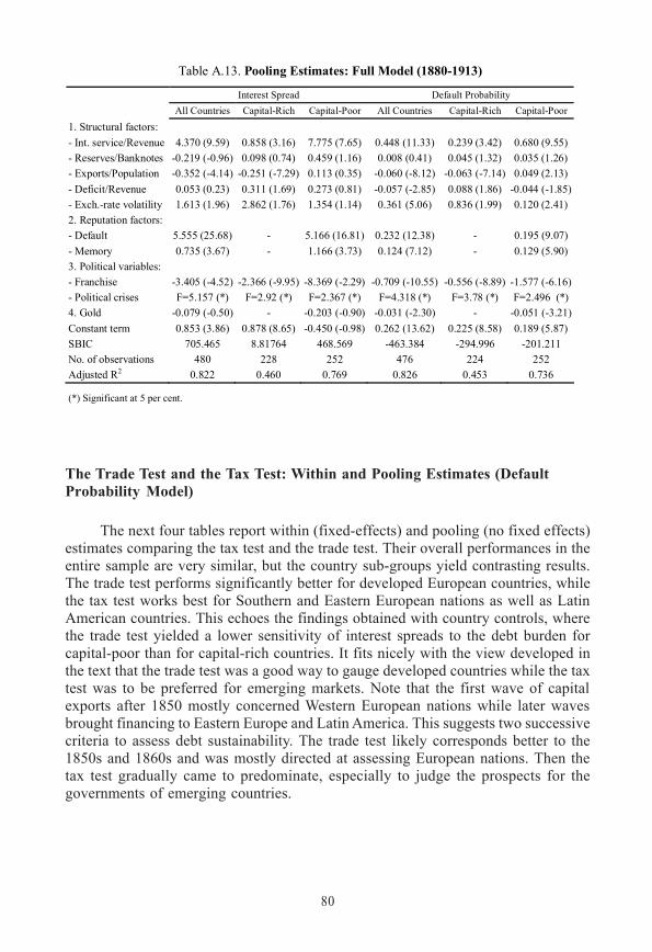
80

Table A.13. Pooling Estimates: Full Model (1880-1913)

Interest Spread Default Probability All Countries Capital-Rich Capital-Poor All Countries Capital-Rich Capital-Poor

1. Structural factors: - Int. service/Revenue 4.370 (9.59) 0.858 (3.16) 7.775 (7.65) 0.448 (11.33) 0.239 (3.42) 0.680 (9.55) - Reserves/Banknotes -0.219 (-0.96) 0.098 (0.74) 0.459 (1.16) 0.008 (0.41) 0.045 (1.32) 0.035 (1.26) - Exports/Population -0.352 (-4.14) -0.251 (-7.29) 0.113 (0.35) -0.060 (-8.12) -0.063 (-7.14) 0.049 (2.13) - Deficit/Revenue 0.053 (0.23) 0.311 (1.69) 0.273 (0.81) -0.057 (-2.85) 0.088 (1.86) -0.044 (-1.85) - Exch.-rate volatility 1.613 (1.96) 2.862 (1.76) 1.354 (1.14) 0.361 (5.06) 0.836 (1.99) 0.120 (2.41) 2. Reputation factors: - Default 5.555 (25.68) - 5.166 (16.81) 0.232 (12.38) - 0.195 (9.07) - Memory 0.735 (3.67) - 1.166 (3.73) 0.124 (7.12) - 0.129 (5.90) 3. Political variables: - Franchise -3.405 (-4.52) -2.366 (-9.95) -8.369 (-2.29) -0.709 (-10.55) -0.556 (-8.89) -1.577 (-6.16) - Political crises F=5.157 (*) F=2.92 (*) F=2.367 (*) F=4.318 (*) F=3.78 (*) F=2.496 (*) 4. Gold -0.079 (-0.50) - -0.203 (-0.90) -0.031 (-2.30) - -0.051 (-3.21) Constant term 0.853 (3.86) 0.878 (8.65) -0.450 (-0.98) 0.262 (13.62) 0.225 (8.58) 0.189 (5.87) SBIC 705.465 8.81764 468.569 -463.384 -294.996 -201.211 No. of observations 480 228 252 476 224 252 Adjusted R2 0.822 0.460 0.769 0.826 0.453 0.736 (*) Significant at 5 per cent.

The Trade Test and the Tax Test: Within and Pooling Estimates (DefaultProbability Model)

The next four tables report within (fixed-effects) and pooling (no fixed effects)estimates comparing the tax test and the trade test. Their overall performances in theentire sample are very similar, but the country sub-groups yield contrasting results.The trade test performs significantly better for developed European countries, whilethe tax test works best for Southern and Eastern European nations as well as LatinAmerican countries. This echoes the findings obtained with country controls, wherethe trade test yielded a lower sensitivity of interest spreads to the debt burden forcapital-poor than for capital-rich countries. It fits nicely with the view developed inthe text that the trade test was a good way to gauge developed countries while the taxtest was to be preferred for emerging markets. Note that the first wave of capitalexports after 1850 mostly concerned Western European nations while later wavesbrought financing to Eastern Europe and Latin America. This suggests two successivecriteria to assess debt sustainability. The trade test likely corresponds better to the1850s and 1860s and was mostly directed at assessing European nations. Then thetax test gradually came to predominate, especially to judge the prospects for thegovernments of emerging countries.

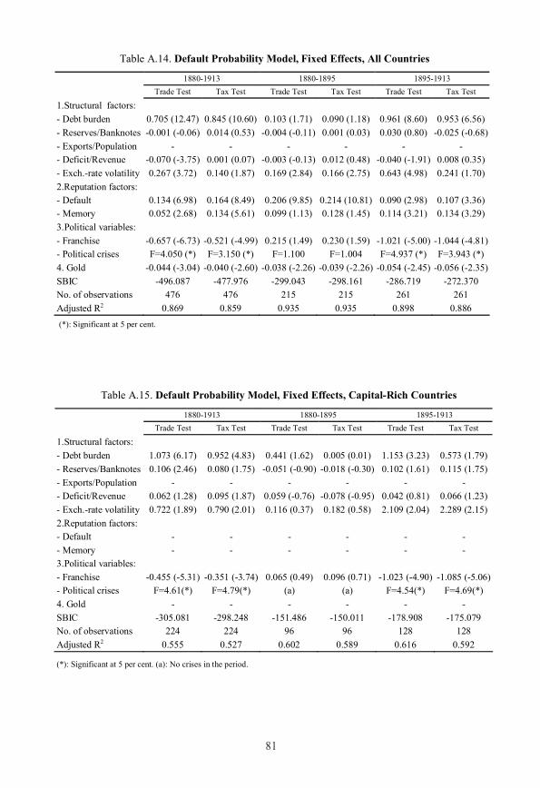
81

Table A.14. Default Probability Model, Fixed Effects, All Countries

1880-1913 1880-1895 1895-1913 Trade Test Tax Test Trade Test Tax Test Trade Test Tax Test

1.Structural factors: - Debt burden 0.705 (12.47) 0.845 (10.60) 0.103 (1.71) 0.090 (1.18) 0.961 (8.60) 0.953 (6.56) - Reserves/Banknotes -0.001 (-0.06) 0.014 (0.53) -0.004 (-0.11) 0.001 (0.03) 0.030 (0.80) -0.025 (-0.68) - Exports/Population - - - - - - - Deficit/Revenue -0.070 (-3.75) 0.001 (0.07) -0.003 (-0.13) 0.012 (0.48) -0.040 (-1.91) 0.008 (0.35) - Exch.-rate volatility 0.267 (3.72) 0.140 (1.87) 0.169 (2.84) 0.166 (2.75) 0.643 (4.98) 0.241 (1.70) 2.Reputation factors: - Default 0.134 (6.98) 0.164 (8.49) 0.206 (9.85) 0.214 (10.81) 0.090 (2.98) 0.107 (3.36) - Memory 0.052 (2.68) 0.134 (5.61) 0.099 (1.13) 0.128 (1.45) 0.114 (3.21) 0.134 (3.29) 3.Political variables: - Franchise -0.657 (-6.73) -0.521 (-4.99) 0.215 (1.49) 0.230 (1.59) -1.021 (-5.00) -1.044 (-4.81) - Political crises F=4.050 (*) F=3.150 (*) F=1.100 F=1.004 F=4.937 (*) F=3.943 (*) 4. Gold -0.044 (-3.04) -0.040 (-2.60) -0.038 (-2.26) -0.039 (-2.26) -0.054 (-2.45) -0.056 (-2.35) SBIC -496.087 -477.976 -299.043 -298.161 -286.719 -272.370 No. of observations 476 476 215 215 261 261 Adjusted R2 0.869 0.859 0.935 0.935 0.898 0.886 (*): Significant at 5 per cent.

Table A.15. Default Probability Model, Fixed Effects, Capital-Rich Countries

1880-1913 1880-1895 1895-1913 Trade Test Tax Test Trade Test Tax Test Trade Test Tax Test

1.Structural factors: - Debt burden 1.073 (6.17) 0.952 (4.83) 0.441 (1.62) 0.005 (0.01) 1.153 (3.23) 0.573 (1.79) - Reserves/Banknotes 0.106 (2.46) 0.080 (1.75) -0.051 (-0.90) -0.018 (-0.30) 0.102 (1.61) 0.115 (1.75) - Exports/Population - - - - - - - Deficit/Revenue 0.062 (1.28) 0.095 (1.87) 0.059 (-0.76) -0.078 (-0.95) 0.042 (0.81) 0.066 (1.23) - Exch.-rate volatility 0.722 (1.89) 0.790 (2.01) 0.116 (0.37) 0.182 (0.58) 2.109 (2.04) 2.289 (2.15) 2.Reputation factors: - Default - - - - - - - Memory - - - - - - 3.Political variables: - Franchise -0.455 (-5.31) -0.351 (-3.74) 0.065 (0.49) 0.096 (0.71) -1.023 (-4.90) -1.085 (-5.06) - Political crises F=4.61(*) F=4.79(*) (a) (a) F=4.54(*) F=4.69(*) 4. Gold - - - - - - SBIC -305.081 -298.248 -151.486 -150.011 -178.908 -175.079 No. of observations 224 224 96 96 128 128 Adjusted R2 0.555 0.527 0.602 0.589 0.616 0.592 (*): Significant at 5 per cent. (a): No crises in the period.

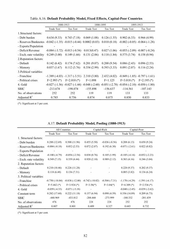
82

Table A.16. Default Probability Model, Fixed Effects, Capital-Poor Countries

1880-1913 1880-1895 1895-1913 Trade Test Tax Test Trade Test Tax Test Trade Test Tax Test

1.Structural factors: - Debt burden 0.634 (9.33) 0.743 (7.18) 0.069 (1.08) 0.126 (1.55) 0.902 (6.33) 0.966 (4.99) - Reserves/Banknotes -0.042 (-1.35) -0.015 (-0.44) 0.0002 (0.03) 0.010 (0.18) -0.002 (-0.05) -0.064 (-1.28) - Exports/Population - - - - - - - Deficit/Revenue -0.084 (-3.72) -0.013 (-0.54) 0.013(0.47) 0.027 (1.06) -0.055 (-2.09) -0.007 (-0.24) - Exch.-rate volatility 0.249 (3.00) 0.149 (1.66) 0.131 (2.06) 0.118 (1.84) 0.575 (3.74) 0.158 (0.94) 2.Reputation factors: - Default 0.142 (6.42) 0.174 (7.62) 0.201 (9.07) 0.200 (9.54) 0.086 (2.43) 0.096 (2.53) - Memory 0.037 (1.67) 0.112 (3.76) 0.354 (2.99) 0.393 (3.33) 0.091 (2.07) 0.116 (2.24) 3.Political variables: - Franchise -1.389 (-4.03) -1.317 (-3.51) 2.310 (3.80) 2.432 (4.02) -0.849 (-1.85) -0.797 (-1.61) - Political crises F=2.993 (*) F=2.010 (*) F=1.098 F=1.125 F=3.018 (*) F=2.195 (*) 4. Gold -0.027 (-1.56) -0.027 (-1.44) -0.048 (-2.60) -0.051 (-2.78) -0.054 (-2.10) -0.050 (-1.80) SBIC -213.674 -198.074 -155.898 -156.637 -114.561 -107.143 No. of observations 252 252 119 119 133 133 Adjusted R2 0.785 0.756 0.874 0.875 0.850 0.833 (*): Significant at 5 per cent.

A.17. Default Probability Model, Pooling (1880-1913)

All Countries Capital-Rich Capital-Poor Trade Test Tax Test Trade Test Tax Test Trade Test Tax Test

1. Structural factors:

- Debt burden 0.288 (12.69) 0.500 (11.96) 0.455 (5.50) -0.036 (-0.56) 0.208 (6.13) 0.650 (9.24)

- Reserves/Banknotes -0.004 (-0.18) 0.052 (2.53) 0.072 (2.07) 0.192 (6.30) -0.071 (-2.61) 0.022 (0.82)

- Exports/Population - - - - - -

- Deficit/Revenue -0.100 (-4.79) -0.054 (-2.54) 0.038 (0.76) 0.105 (1.99) -0.105 (-4.14) -0.052 (-2.23)

- Exch.-rate volatility 0.549 (7.15) 0.339 (4.44) 0.920 (2.10) 0.989 (2.12) 0.383 (4.16) 0.246 (3.04)

2. Reputation factors:

- Default 0.210 (10.46) 0.226 (11.28) - - 0.220 (9.37) 0.202 (9.37)

- Memory 0.118 (6.48) 0.136 (7.31) - - 0.085 (3.82) 0.136 (6.24)

3. Political variables:

- Franchise -0.750 (-10.84) -0.838 (-12.00) -0.742 (-10.02) -0.504 (-7.31) -1.170 (-4.29) -1.591 (-6.17)

- Political crises F=5.462 (*) F=3.924 (*) F=3.58(*) F=3.04(*) F=4.309 (*) F=2.536 (*)

4. Gold -0.059 (-4.33) -0.071 (-5.18) - - -0.040 (-2.45) -0.039 (-2.62)

Constant term 0.282 (17.60) 0.222 (11.18) 0.157 (6.94) 0.098 (4.59) 0.356 (14.89) 0.209 (6.73)

SBIC -440.969 -433.812 -288.468 -273.999 -180.332 -201.439

No. of observations 476 476 224 224 252 252

Adjusted R2 0.807 0.801 0.409 0.327 0.683 0.732 (*): Significant at 5 per cent.

83

Robustness Tests: Endogeneity and Auto-correlation

GMM estimates

Possible Problems. The presence of endogeneity problems constitutes one potentialflaw in the estimates in Sections VI and VII of the main text. For instance, if debt ispermanently re-contracted, higher borrowing rates result in larger debt burdens, butthis increases the probability of default and thus the interest rate. If this were the case,then the estimates of the elasticity of the interest-rate spreads (or default probabilities)to the interest burden would be biased upward1. This could arise in a context of creditrationing à la Stiglitz and Weiss (1981)2. In their model of permanent debt re-contracting, the non-linearity of interest rate spreads in terms of credit rating resultsbecause an increased interest rate raises the interest-service burden, which in turnincreases the likelihood of default and thus the interest rate. This result, however,depends heavily on the time horizon of the debt contract. In the world under study,the debt burden was a weighted average of past interest rates corresponding to anextended period. This kind of endogeneity therefore is not a serious problem becausethe long maturity of public debts in the period implies that the (marginal) borrowingpremium had only a marginal effect on the (average) current debt burden. A typicalloan would represent only between (at most) 5 per cent and 10 per cent of theoutstanding debt, often much less, so that its effect on the debt burden would have tobe divided by 10 or 20. In other words, a feedback did exist, but it was very small andcan safely be ignored.

More important, the null hypothesis is that people looked at the debt burden asa straight determinant of the probability of default. Sections VI and VII tested whetherthis theory of the pricing of risk by investors is correct. That investors were themselvesright or wrong to adhere to such views is another question on which this study haslittle to say. In addition, standard procedures to handle endogeneity require makingspecific assumptions on the kind of endogeneity that needs to be corrected. For instance,the so-called Instrumental Variable technique requires finding variables with specificproperties in view of the problems at hand. Yet without evidence on contemporaryconcerns regarding this problem it is not clear how one should proceed. In the endthere is no reason to superimpose another reasoning on that of the time.

For those who would want to see more, however, and because the results reportedhere would benefit from additional evidence, several robustness tests were performed.This section seeks to replicate the estimation performed earlier, using an alternativeestimation technique known as the Generalised Method of Moments (GMM). GMMestimates have the considerable advantage that they correct for a variety of potentialproblems (including endogeneity) without requiring the use of extra variables. Theyachieve this by making intensive use of the information contained in the variablesalready in the model. The “instruments” used are combinations of the basic explanatoryvariables themselves. In that respect, GMM may be thought of as just another estimationtechnique. We do not know that people had in mind some specific least-squares

84

technique. We know only that they thought that some variables influencedcreditworthiness and that there are reasons to believe that this should be reflected inthe prices of bonds. In other words, to remain agnostic about the precise estimationtechnique, as one logically should, it seems natural to try alternative estimates, just tomake sure. This should provide everybody with comfort.

Technical Treatment. If feedbacks from the marginal borrowing rate to the debtburden do matter, neither OLS nor GLS panel techniques provide consistent estimates,but GMM estimators do. Defining the relevant GMM procedure depends strongly onthe type of problem faced. Alternative model specifications give rise to alternativesets of orthogonality restrictions on which estimations may be based3. Increasing thenumber of conditions normally induces an improvement in the precision of theestimators. On the other hand, this can make the size of the problem somewhat time-consuming for conventional software packages. The question becomes one of strikinga balance between efficiency and practicality (Mátyás and Sevestre, 1996).

This study relies on a technique suggested by Arellano and Bond (1991). Theypropose obtaining efficient estimators by working with the model in first differences.Their application of GMM points to using lagged values of the explanatory variablesin levels as instruments, but this widely used linear GMM has been found to display alarge finite sample bias and poor precision in simulation studies (Alonso-Borrego andArellano, 1999). This occurs because lagged levels of the explanatory variables provideweak instruments for first differences in this case4. Blundell and Bond (1998) consideran alternative estimator. They take lagged differences of the variables as instrumentsand work with equations in levels. Mátyás and Sevestre (1996) show that thisspecification has the further advantage of controlling for serial correlation in theresiduals. In the present case, the estimators obtained from the equation in levels,where the instruments are first-difference variables, were found to be efficient5.

The results presented in Table A.18 rely on these two alternative procedures:Arellano-Bond and the model in levels. Estimates are reported for the model’s mostcomprehensive form. Each column corresponds to alternative estimation techniques,with the column indicating the procedure that has been followed in each case6. Theresults confirm earlier findings. The most robust variables turn out to be the classicdebt burden, debt default and memory variables. The elasticity parameters for othervariables appear less stable, with the effect of gold, for instance, jumping aroundsomewhat (it is positive in some equations, negative in others and often not significant).This generally confirms the earlier interpretations and shows that the main results andconclusions are unaffected by the precise estimation technique. The extent of theendogeneity problem, if it does exist, must be quite limited.

85

Table A.18. GMM Estimates, Fixed Effects, All Countries

Model I: Interest-Rate Spreads Model II: Default Probability Model in levels Arellano-Bond Model in levels Arellano-Bond

1. Structural factors: - Interest service/Tax revenue 8.824 (14.71) 7.193 (23.55) 0.786 (10.65) 0.883 (12.67) - Reserves/Banknotes -0.354 (-1.57) -0.685 (-3.07) 0.024 (0.93) -0.075 (-2.64) - Exports/Population 1.052 (6.46) 0.496 (2.95) 0.075 (4.53) 0.053 (3.07) - Deficit/Revenue 0.887 (6.83) 0.514 (8.77) 0.021 (2.08) 0.012 (3.36) - Exch.-rate volatility 1.204 (9.23) 0.905 (2.02) 0.164 (4.51) 0.134 (2.47) 2. Reputation factors: - Default 4.780 (31.67) 2.766 (26.15) 0.135 (10.26) 0.084 (10.42) - Memory (T= 0.1) 0.584 (3.21) 1.056 (3.17) 0.124 (7.87) 0.131 (2.08) 3. Political variables: - Franchise -3.487 (-3.13) -4.320 (-2.12) -0.314 (-2.82) 0.427 (1.35) 4. Gold: 0.423 (2.06) 0.274 (1.24) -0.065 (-2.51) -0.027 (-1.85) No. of observations 464 464 460 460 Standard Errors computed from heteroscedasticity-consistent matrix (Robust-White). Instruments used in GMM: lag 1 and 2 instruments. The Ȥ2 test, in connection with GMM, led to the choice of the appropriate matrix of instruments (described by a lag order which, as can be seen, always corresponds to weak exogeneity of the instruments). See the explanatory endnote 5.

Instrumental Variable (IV) Estimations

The tables below present the results from using the standard IV technique totackle endogeneity. This technique amounts to looking for a set of instrumental variableswhose number must at least equal the number of regressors in the model and whichmust satisfy two conditions — they must be uncorrelated with the disturbances, atleast asymptotically, and they must be asymptotically correlated with the explanatoryvariables. The problems lie in the determination of the instrumental variables. Asargued in the main text it is not clear what the instruments should be, given theperceptions of the time. The following merely employs some conventional recipesthat apply to the most usual situations. Two alternative lists of instruments have beenconsidered. The first (List 1) comprises a constant term, a time trend, the laggedburden of interest service for each country, populations, the rates of growth ofpopulations and lagged degrees of openness (exports divided by GDPs). The second(List 2) comprises a time trend, the lagged burden of interest service for each country,the rates of growth of populations and three lagged explanatory variables.

86

Table A.19. Interest-Rate Spread Model, All Countries, (Fixed Effects)

Benchmark a Instrumented List 1 Instrumented List 2

1. Structural factors: - Interest service/Tax revenue 8.172 (8.68) 6.780 (5.79) 7.185 (6.50) - Reserves/Banknotes -0.226 (-0.74) -0.415 (-1.13) -0.347 (-0.95) - Exports/Reserves 0.772 (1.94) 0.664 (1.26) 0.657 (1.22) - Deficit/Revenue 0.766 (3.31) -0.140 (-0.29) 0.011 (0.03) - Exch.-rate volatility 1.147 (1.29) 0.896 (0.69) 0.345 (0.27) 2. Reputation factors: - Default 4.793 (21.07) 5.123 (22.52) 5.067 (22.08) - Memory 0.758 (2.66) 0.314 (1.08) 0.377 (1.26) 3. Political variables: - Franchise -2.485 (-1.76) -3.014 (-1.91) -2.841 (-1.79) - Political crises F=3.706 (*) F=4.672 (*) F=4.442 (*) 4. Gold adherence: 0.060 (0.33) 0.071 (0.39) 0.032 (0.17) SBIC 677.625 695.401 693.832 Adjusted R2 0.856 0.845 0.846 Number of observations: 464. (*) significant at 5 per cent. a) The benchmark is obtained with direct ordinary least square techniques as in Table A.1 column 5, but with the same data as for the instrumented regressions above. Since instrumental variable regressions require dropping observations, the benchmark estimates do not exactly coincide with the results in Table A.1 column 5, but are very close to them.

Table A.20. Interest-Rate Spread Model, Capital-Rich Countries (Fixed Effects)

Benchmark a Instrumented List 1 Instrumented List 2

1. Structural factors: - Interest service/Tax revenue 4.111 (6.03) 5.319 (6.82) 5.963 (7.48) - Reserves/Banknotes 0.233 (1.34) 0.080 (0.33) -0.006 (-0.02) - Exports/Reserves -0.153 (-1.29) -0.172 (-1.14) -0.056 (-0.36) - Deficit/Revenue 0.305 (1.61) 0.407 (1.42) 0.572 (2.00) - Exch.-rate volatility 2.772 (1.91) 9.979 (3.12) 9.663 (3.13) 2. Reputation factors: - Default - - - - Memory - - - 3. Political variables: - Franchise -0.874 (-2.18) -0.532 (-1.36) -0.744 (-1.74) - Political crises F=2.76(*) F=4.33(*) F=2.97(*) 4. Gold adherence: - - - SBIC -2.21268 -16.2957 -18.9290 Adjusted R2 0.581 0.632 0.640 Number of observations: 220. (*) significant at 5 per cent. a) The benchmark is obtained with direct ordinary least square techniques as in Table A.2 column 5, but with the same data as for the instrumented regressions above. Since instrumental variable regressions require dropping observations, the benchmark estimates do not exactly coincide with the results in Table A.2 column 5, but are very close to them.

87

Table A.21. Interest-Rate Spread Model, Capital-Poor Countries (Fixed Effects)

Benchmark a Instrumented List 1 Instrumented List 2

1. Structural factors: - Interest service/Tax revenue 8.361 (5.66) 5.255 (2.69) 6.342 (3.55) - Reserves/Banknotes -0.277 (-0.57) -0.783 (-1.33) -0.591 (-1.02) - Exports/Reserves 3.219 (2.57) 4.255 (2.09) 3.474 (1.66) - Deficit/Revenue 0.807 (2.38) -0.549 (-0.72) -0.187 (-0.29) - Exch.-rate volatility 1.617 (1.27) 2.360 (1.19) 1.481 (0.75) 2. Reputation factors: - Default 4.885 (15.14) 5.189 (16.16) 5.147 (15.75) - Memory 0.803 (1.88) 0.145 (0.33) 0.308 (0.68) 3. Political variables: - Franchise -5.900 (-1.10) -9.043 (-1.61) -7.331 (-1.31) - Political crises F=1.836 (*) F=2.352 (*) F=2.181 (*) 4. Gold adherence: 0.054 (0.21) 0.103 (0.39) 0.062 (0.23) SBIC 453.538 464.466 464.814 Adjusted R2 0.804 0.786 0.785 Number of observations: 244. (*) significant at 5 per cent. a) The benchmark is obtained with direct ordinary least square techniques as in Table A.3 column 5, but with the same data as for the instrumented regressions above. Since instrumental variable regressions require dropping observations, the benchmark estimates do not exactly coincide with the results in Table A.3 column 5, but are very close to them.

Dealing with Auto-correlation

Owing to the high persistence of the debt burden variables for the reasonsdiscussed above, the explanatory variables do exhibit auto-correlation, as do yieldpremiums. In this context, tests suggest auto-correlation in the residuals. Earlier resultsare nonetheless robust to such phenomena. This can be seen from a variety ofperspectives. First, because the regression output from GMM estimates on firstdifferences (à la Arellano-Bond) barely differed from earlier results, the potentialnuisance of auto-correlation problems is limited. Moreover, there are two other waysto deal with this and show that the results remain robust.

Random effects. The basic assumption in the random effects model is that theregression disturbance is composed of two independent components. First, eachobservation is affected by a shock that is independent and identically distributed acrosscountries and time. Second, cross-sectional units (countries) are affected by adisturbance whose correlation remains unchanged over time. This structure enablescontrolling for auto-correlation when the usual assumption of a geometrically decayinginfluence of past disturbances is doubtful. As the three tables below show, the resultsfor both models using this approach resemble closely those reported in previous tables.

88

Tabl

e A

.22.

All

Cou

ntri

es (R

ando

m E

ffec

ts)

In

tere

st-R

ate

Spre

ad M

odel

D

efau

lt Pr

obab

ility

Mod

el

18

80-1

913

1880

-189

5 18

95-1

913

1880

-191

3 18

80-1

895

1895

-191

3

1. S

truct

ural

fact

ors:

- I

nter

est s

ervi

ce/R

even

ue

6.41

4 (9

.35)

5.

080

(5.3

0)

5.25

8 (5

.00)

0.

680

(11.

30)

0.22

8 (3

.85)

0.

624

(5.9

6)

- Res

erve

s/B

ankn

otes

-0

.301

(-1.

09)

-0.3

35 (-

0.62

) -0

.536

(-1.

59)

0.00

7 (0

.28)

-0

.066

(-2.

01)

0.00

09 (0

.03)

- E

xpor

ts/P

opul

atio

n -0

.131

(-0.

73)

-0.7

74 (-

2.67

) -0

.026

(-0.

14)

-0.0

37 (-

2.34

) -0

.119

(-6.

11)

0.01

0 (0

.49)

- D

efic

it/R

even

ue.

0.56

7 (2

.52)

1.

138

(3.0

1)

0.08

0 (0

.34)

-0

.014

(-0.

72)

-0.0

15 (-

0.69

) -0

.007

(-0.

31)

- Exc

h.-r

ate

vola

tility

1.

193

(1.4

1)

1.76

1 (1

.83)

4.

450

(3.0

4)

0.19

5 (2

.67)

0.

182

(3.2

0)

0.39

7 (2

.93)

2.

Rep

utat

ion

fact

ors:

- D

efau

lt 4.

989

(23.

17)

5.41

5 (1

8.27

) 3.

740

(11.

64)

0.18

2 (9

.76)

0.

209

(11.

84)

0.14

8 (4

.95)

- M

emor

y

0.56

9 (2

.47)

1.

441

(1.8

2)

0.08

5 (0

.25)

0.

113

(5.6

3)

0.15

8 (3

.06)

0.

111

(3.3

7)

3. P

oliti

cal v

aria

bles

:

- F

ranc

hise

-2

.340

(-2.

14)

0.23

8 (0

.12)

-4

.968

(-3.

10)

-0.5

94 (-

6.23

) 0.

101

(0.8

4)

-1.0

54 (-

6.62

) - P

oliti

cal c

rises

F=

6.03

(*)

F=2.

946

(*)

F=3.

673

(*)

F=5.

181

(*)

F=3.

092

(*)

F=3.

188

(*)

4. G

old:

0.

028

(0.1

6)

-0.3

40 (-

1.29

) 0.

193

(0.8

0)

-0.0

37 (-

2.54

) -0

.045

(-2.

87)

-0.0

52 (-

2.33

) C

onst

ant

0.25

3 (0

.81)

1.

134

(2.5

3)

0.50

2 (1

.04)

0.

202

(7.3

5)

0.39

8 (1

4.23

) 0.

207

(4.3

5)

Hau

sman

test

Ȥ2 (1

5)=2

6.64

2 (*

) Ȥ2 (1

1)=1

9.46

8(*)

Ȥ2 (1

6)=2

9.94

5(*)

Ȥ2 (1

5)=3

0.42

1 (*

) Ȥ2 (1

1)=3

7.83

2(*)

Ȥ2 (1

5)=3

4.59

9(*)

N

o. o

f obs

erva

tions

48

0 21

5 26

5 47

6 21

5 26

1 A

djus

ted

R2 0.

805

0.82

7 0.

799

0.80

1 0.

853

0.77

9 (*

): Si

gnifi

cant

at 5

per

cen

t. Th

e H

ausm

an te

st fo

r Ran

dom

Effe

cts

vers

us F

ixed

Effe

cts g

ener

ally

cho

oses

Fix

ed E

ffect

s.

89

Tabl

e A

.23.

Cap

ital-R

ich

Cou

ntri

es (R

ando

m E

ffect

s)

In

tere

st-Ra

te S

prea

d M

odel

D

efau

lt Pr

obab

ility

Mod

el

18

80-1

913

1880

-189

5 18

95-1

913

1880

-191

3 18

80-1

895

1895

-191

3

1.St

ruct

ural

fact

ors:

- I

nter

est s

ervi

ce/R

even

ue

2.04

2 (4

.66)

0.

426

(0.6

7)

1.29

7 (1

.97)

0.

352

(3.3

3)

-0.0

75 (-

0.51

) 0.

373

(1.9

6)

- Res

erve

s/B

ankn

otes

0.

211

(1.3

5)

-0.1

76 (-

0.96

) 0.

360

(1.7

9)

0.07

1 (1

.72)

-0

.015

(-0.

33)

0.09

9 (1

.65)

- E

xpor

ts/P

opul

atio

n -0

.261

(-4.

15)

-0.4

48 (-

5.04

) -0

.043

(-0.

56)

-0.0

62 (-

4.28

) -0

.080

(-3.

89)

-0.0

17 (-

0.82

) - D

efic

it/R

even

ue

0.23

7 (1

.31)

-0

.101

(-0.

36)

0.18

2 (1

.049

) 0.

076

(1.5

5)

-0.0

32 (-

0.47

) 0.

061

(1.1

8)

- Exc

h.-ra

te v

olat

ility

2.

940

(2.0

5)

1.06

1 (0

.91)

4.

647

(1.3

8)

0.84

6 (2

.15)

0.

259

(0.8

9)

2.22

8 (2

.10)

2.

Rep

utat

ion

fact

ors:

- D

efau

lt -

- -

- -

- - M

emor

y

- -

- -

- -

3.Po

litic

al v

aria

bles

:

- F

ranc

hise

-1

.433

(-4.

64)

-0.0

05 (-

1.04

) -2

.889

(-5.

15)

-0.4

41 (-

5.65

) 0.

002

(0.0

2)

-0.9

21 (-

5.74

) - P

oliti

cal c

rises

F=

3.85

(*)

(a)

F= 5

.21

(*)

F=4.

43 (*

) (a

) F=

5.08

(*)

4. G

old:

-

- -

- -

- C

onst

ant

0.55

1 (3

.89)

1.

253

(7.7

3)

0.41

8 (2

.22)

0.

176

(4.9

9)

0.31

3 (8

.09)

0.

141

(2.6

4)

Hau

sman

test

Ȥ2 (7

)=25

.516

(*)

Ȥ2 (7)=

25.5

16 (*

) Ȥ2 (7

)=14

.228

(*)

Ȥ2 (7)=

17.2

00 (*

) Ȥ2 (6

)=13

.019

(*)

Ȥ2 (7)=

13.6

81

No.

of o

bser

vatio

ns

228

96

132

224

96

128

Adj

uste

d R

2 0.

297

0.41

5 0.

315

0.42

0 0.

429

0.34

5 (*

): Si

gnifi

cant

at 5

per

cen

t. (a

): N

o cr

ises i

n th

e pe

riod.

The

Hau

sman

test

for R

ando

m E

ffect

s ver

sus F

ixed

Effe

cts

gene

rally

cho

oses

Fix

ed E

ffect

s.

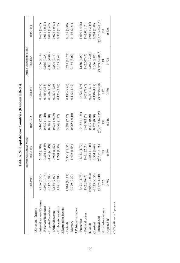
90

Tabl

e A

.24.

Cap

ital-P

oor

Cou

ntri

es (R

ando

m E

ffec

ts)

In

tere

st R

ate

Spre

ad M

odel

D

efau

lt Pr

obab

ility

Mod

el

18

80-1

913

1880

-189

5 18

95-1

913

1880

-191

3 18

80-1

895

1895

-191

3

1.St

ruct

ural

fact

ors:

- I

nter

est s

ervi

ce/R

even

ue

7.80

6 (6

.55)

6.

162

(3.8

0)

5.46

6 (2

.39)

0.

704

(8.5

9)

0.16

6 (2

.14)

0.

627

(3.6

7)

- Res

erve

s/B

ankn

otes

-0

.063

(-0.

14)

-0.3

16 (-

0.29

) -0

.637

(-1.

10)

0.00

5 (0

.15)

0.

015

(0.2

8)

-0.0

11 (-

0.23

) - E

xpor

ts/P

opul

atio

n 0.

517

(0.9

4)

-1.4

0 (-1

.49)

0.

687

(1.1

0)

0.06

0 (1

.74)

-0

.001

(-0.

02)

0.08

1 (1

.67)

- D

efic

it/R

even

ue

0.68

4 (2

.07)

0.

995

(1.8

2)

-0.0

34 (-

0.09

) -0

.023

(-0.

98)

0.00

4 (0

.14)

-0

.026

(-0.

93)

- Exc

h.-ra

te v

olat

ility

1.

081

(0.9

1)

1.74

9 (1

.30)

3.

648

(1.7

2)

0.17

3 (2

.06)

0.

155

(2.4

8)

0.33

5 (2

.12)

2.

Rep

utat

ion

fact

ors:

- D

efau

lt 4.

914

(16.

17)

5.33

0 (1

2.55

) 3.

597

(7.5

2)

0.18

3 (8

.46)

0.

215

(10.

75)

0.13

9 (3

.89)

- M

emor

y 0.

799

(2.2

2)

1.49

2 (1

.64)

-0

.065

(-0.

10)

0.11

2 (4

.49)

0.

164

(3.0

2)

0.10

3 (2

.21)

3.

Polit

ical

var

iabl

es:

- Fra

nchi

se

-7.4

93 (-

1.73

) 14

.313

(1.7

9)

-10.

156

(-1.

85)

-1.4

72 (-

4.94

) 1.

656

(4.0

0)

-1.6

90 (-

4.08

) - P

oliti

cal c

rises

F=

2.37

6 (*

) F=

3.12

2 (*

) F=

1.98

1 (*

) F=

2.87

1 (*

) F=

2.50

7 (*

) F=

2.00

1 (*

) 4.

Gol

d:

0.00

04 (0

.002

) -0

.553

(-1.

45)

0.11

2 (0

.30)

-0

.037

(-2.

16)

-0.0

43 (-

2.38

) -0

.059

(-2.

14)

Con

stan

t -0

.325

(-0.

56)

0.53

4 (0

.69)

0.

523

(0.5

0)

0.19

0 (4

.89)

0.

356

(8.8

5)

0.20

4 (2

.58)

H

ausm

an te

st

Ȥ2 (7)=

11.4

10

Ȥ2 (8)=

14.7

81

Ȥ2 (7)=

14.6

26 (*

) Ȥ2 (7

)=10

.008

Ȥ2 (7

)=17

.930

(*)

Ȥ2 (7)=

19.4

98 (*

) N

o. o

f obs

erva

tions

25

2 11

9 13

3 25

2 11

9 13

3 A

djus

ted

R2 0.

759

0.79

6 0.

748

0.73

0 0.

724

0.72

6 (*

): Si

gnifi

cant

at 5

per

cen

t.

91

Kmenta-type error structure. The second way to deal with auto-correlation is torely on the so-called Kmenta-type error structure (Kmenta, 1986). This alternativespecification is superior to the crude AR1 structure because it allows for differentauto-regressive components across equations and for heteroscedastic disturbances. Itis based on the auto-correlation of time series and the heteroscedasticity of cross-sections. Therefore, pooled time series of cross-sections should be both auto-correlatedtime-wise and cross-sectionally heteroscedastic (Kmenta, 1986). Economists usepooling techniques, error components and Kmenta-type error structures, althoughthey differ in the assumptions imposed on the disturbances. The usual error componentsmodel has homoscedastic disturbances, whereas the Kmenta technique hasheteroscedastic ones. Both techniques allow for serial correlation, but in the usualerror-components model this serial correlation is constant across time, whereas itdecays over time with the Kmenta technique. The advantage of both methods residesin the gains from pooling a larger data set and more variation to explain the underlyingeconomic relationship. A test for choosing among the two alternatives should be basedon the conditional moments of the data. These approaches may lead to a betterformulation of a model for pooled time series of cross-section data7.

The results (Table A.25 below) do suggest some auto-correlation, although it variessubstantially across countries. Note that no systematic pattern is visible among sub-groups of countries. While the estimated debt burden coefficient is sometimes slightlyreduced (from 0.847 to 0.679 in the default probability model) its significance andeffect remain very large. Moreover, the other conclusions outlined earlier still hold.

Table A.25. Kmenta’s Model, 1880-1913

Pooling Fixed Effects Interest-Rate Spread

Model Default Probability

Model Interest-Rate Spread

Model Default Probability

Model

1. Structural factors: - Interest service/Revenue 3.448 (6.67) 0.490 (5.67) 6.590 (7.86) 0.679 (5.63) - Reserves/Banknotes -0.170 (-2.57) -0.008 (-0.61) -0.023 (-0.11) 0.004 (0.16) - Exports/Population -0.182 (-1.65) -0.048 (-3.19) -0.965 (-3.15) -0.046 (-0.72) - Deficit/Revenue -0.039 (-0.34) 0.003 (0.15) -0.200 (-1.03) -0.018 (-1.08) - Exch.-rate volatility 0.612 (3.46) 0.074 (1.93) 0.918 (2.43) 0.082 (1.05) 2. Reputation factors: - Default 3.602 (0.26) 0.132 (1.27) 1.385 (2.04) 0.093 (1.99) - Memory 1.165 (0.10) 0.127 (1.28) 1.411 (2.23) 0.144 (2.67) 3. Political variables: - Franchise -5.496 (-4.74) -1.101 (-6.78) -0.423 (-1.60) -0.392 (-2.81) - Political crises F= 4.12 (*) F=3.47 (*) F=2.98 (*) F=3.71 (*) 4. Gold: 0.199 (3.00) 0.005 (0.44) -0.080 (-4.54) -0.030 (-3.51) Constant 0.865 (6.57) 0.260 (11.20) - - No. of observations 480 476 480 476 Adjusted R2 0.877 0.905 0.891 0.871

(*): Significant at 5 per cent.

Note: Compare Pooling with Table A.13 (columns “all countries”) and Fixed Effects with the last columns of Tables A.1 and A.4.

92

Political Variables

The following table reports the parameter estimates for political variables. Politicalvariables are introduced as dummies taking a value of one for a given time and country.For each event, the time and country concerned are indicated in the table. The resultscorrespond to regression output when political variables are added (column 5 inTables A.1 and A.4).

A number of the political crises had large and significant effects. Unsurprisingly,they corresponded to the main political events of the time. Wars increased premiums,especially for the defeated (Spain against the United States, Russia against Japan).The victors occasionally benefited (e.g. the Balkan wars for Greece). Revolts andcoups deteriorate credit (Brazil in 1893, Russia in 1906). Transition to greaterdemocracy improves it (Portugal, 1910). The effects of the Boer War, which targetedall countries (because they affected Britain and thus all yields measured against Britain’s)had the effect of deteriorating borrowing terms (marginally, but in the defaultprobability model significantly). This may be understood as a kind of flight to quality,where the increased borrowing needs of one prominent supplier of capital make accessto credit in the rest of the world more costly.

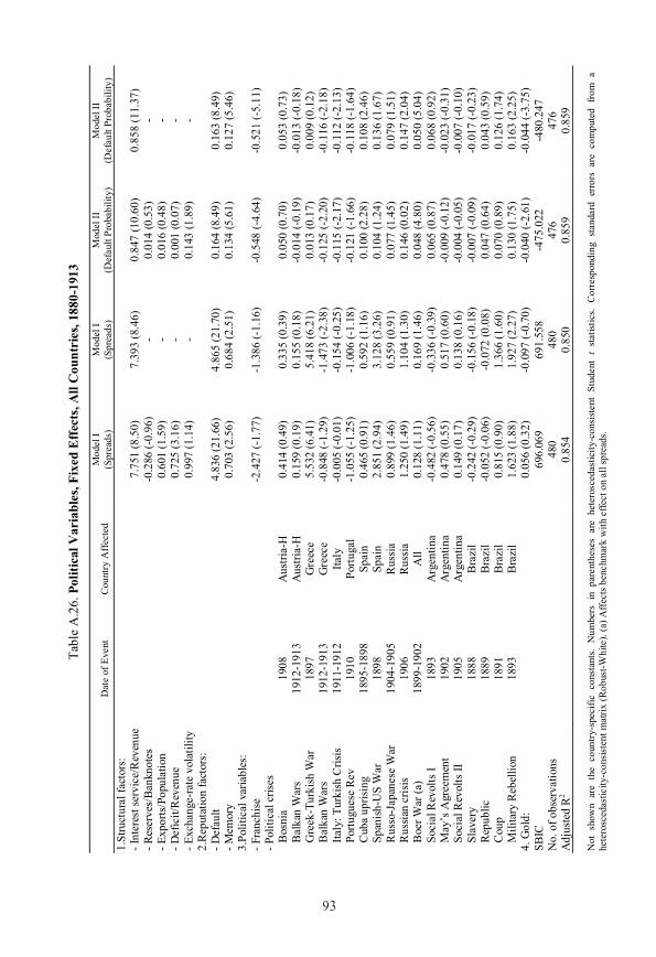
93

Tabl

e A

.26.

Pol

itica

l Var

iabl

es, F

ixed

Eff

ects

, All

Cou

ntri

es, 1

880-

1913

D

ate

of E

vent

Co

untry

Affe

cted

M

odel

I

(Spr

eads

) M

odel

I

(Spr

eads

) M

odel

II

(Def

ault

Prob

abili

ty)

Mod

el II

(D

efau

lt Pr

obab

ility

) 1.

Stru

ctur

al fa

ctor

s:

- Int

eres

t ser

vice

/Rev

enue

7.

751

(8.5

0)

7.39

3 (8

.46)

0.

847

(10.

60)

0.85

8 (1

1.37

) - R

eser

ves/

Ban

knot

es

-0.2

86 (-

0.96

) -

0.01

4 (0

.53)

-

- Exp

orts

/Pop

ulat

ion

0.60

1 (1

.59)

-

0.01

6 (0

.48)

-

- Def

icit/

Rev

enue

0.

725

(3.1

6)

- 0.

001

(0.0

7)

- - E

xcha

nge-

rate

vol

atili

ty

0.99

7 (1

.14)

-

0.14

3 (1

.89)

-

2.R

eput

atio

n fa

ctor

s:

- Def

ault

4.83

6 (2

1.66

) 4.

865

(21.

70)

0.16

4 (8

.49)

0.

163

(8.4

9)

- Mem

ory

0.

703

(2.5

6)

0.68

4 (2

.51)

0.

134

(5.6

1)

0.12

7 (5

.46)

3.

Polit

ical

var

iabl

es:

- Fra

nchi

se

-2.4

27 (-

1.77

) -1

.386

(-1.

16)

-0.5

48 (-

4.64

) -0

.521

(-5.

11)

- Pol

itica

l cris

es

Bos

nia

1908

A

ustri

a-H

0.

414

(0.4

9)

0.33

5 (0

.39)

0.

050

(0.7

0)

0.05

3 (0

.73)

B

alka

n W

ars

1912

-191

3 A

ustri

a-H

0.

159

(0.1

9)

0.15

5 (0

.18)

-0

.014

(-0.

19)

-0.0

13 (-

0.18

) G

reek

-Tur

kish

War

18

97

Gre

ece

5.53

2 (6

.41)

5.

418

(6.2

1)

0.01

3 (0

.17)

0.

009

(0.1

2)

Bal

kan

War

s 19

12-1

913

Gre

ece

-0.8

48 (-

1.29

) -1

.473

(-2.

38)

-0.1

25 (-

2.20

) -0

.116

(-2.

18)

Italy

: Tur

kish

Cris

is

1911

-191

2 Ita

ly

-0.0

05 (-

0.01

) -0

.154

(-0.

25)

-0.1

15 (-

2.17

) -0

.112

(-2.

13)

Portu

gues

e R

ev

1910

Po

rtuga

l -1

.055

(-1.

25)

-1.0

06 (-

1.18

) -0

.121

(-1.

66)

-0.1

18 (-

1.64

) C

uba

upris

ing

1895

-189

8 Sp

ain

0.46

5 (0

.91)

0.

592

(1.1

6)

0.10

0 (2

.28)

0.

108

(2.4

6)

Span

ish-

US

War

18

98

Spai

n 2.

851

(2.9

4)

3.12

8 (3

.26)

0.

104

(1.2

4)

0.13

6 (1

.67)

R

usso

-Jap

anes

e W

ar

1904

-190

5 R

ussi

a 0.

899

(1.4

6)

0.55

9 (0

.91)

0.

077

(1.4

5)

0.07

9 (1

.51)

R

ussi

an c

risis

19

06

Rus

sia

1.25

0 (1

.49)

1.

104

(1.3

0)

0.14

6 (0

.02)

0.

147

(2.0

4)

Boe

r War

(a)

1899

-190

2 A

ll 0.

128

(1.1

1)

0.16

9 (1

.46)

0.

048

(4.8

0)

0.05

0 (5

.04)

So

cial

Rev

olts

I 18

93

Arg

entin

a -0

.482

(-0.

56)

-0.3

36 (-

0.39

) 0.

065

(0.8

7)

0.06

8 (0

.92)

M

ay’s

Agr

eem

ent

1902

A

rgen

tina

0.47

8 (0

.55)

0.

517

(0.6

0)

-0.0

09 (-

0.12

) -0

.023

(-0.

31)

Soci

al R

evol

ts II

19

05

Arg

entin

a 0.

149

(0.1

7)

0.13

8 (0

.16)

-0

.004

(-0.

05)

-0.0

07 (-

0.10

) Sl

aver

y 18

88

Bra

zil

-0.2

42 (-

0.29

) -0

.156

(-0.

18)

-0.0

07 (-

0.09

) -0

.017

(-0.

23)

Rep

ublic

18

89

Bra

zil

-0.0

52 (-

0.06

) -0

.072

(0.0

8)

0.04

7 (0

.64)

0.

043

(0.5

9)

Cou

p 18

91

Bra

zil

0.81

5 (0

.90)

1.

366

(1.6

0)

0.07

0 (0

.89)

0.

126

(1.7

4)

Mili

tary

Reb

ellio

n 18

93

Bra

zil

1.62

3 (1

.88)

1.

927

(2.2

7)

0.13

0 (1

.75)

0.

163

(2.2

5)

4. G

old:

0.

056

(0.3

2)

-0.0

97 (-

0.70

) -0

.040

(-2.

61)

-0.0

44 (-

3.75

) SB

IC

696.

069

691.

558

-475

.022

-4

80.2

47

No.

of o

bser

vatio

ns

480

480

476

476

Adj

uste

d R

2

0.

854

0.85

0 0.

859

0.85

9 N

ot s

how

n ar

e th

e co

untry

-spe

cific

con

stan

ts. N

umbe

rs i

n pa

rent

hese

s ar

e he

tero

sced

astic

ity-c

onsi

stent

Stu

dent

t s

tatis

tics.

Corre

spon

ding

sta

ndar

d er

rors

are

com

pute

d fro

m a

he

tero

sced

astic

ity-c

onsis

tent

mat

rix (R

obus

t-Whi

te).

(a) A

ffect

s ben

chm

ark

with

effe

ct o

n al

l spr

eads

.

94

Notes

1. S, the burden of interest service, is equal to rD, where r is the apparent interest rate onthe public debt and D is the nominal debt. If all the debt were short term, then r wouldalso equal i, the actual rate on the public debt, and one would have i-i* as l.h.v. andiD as r.h.v., which would raise substantial problems. Because most debts were longterm, however, the relation between the i and the r is that between the marginal costof borrowing (i) and the average cost of borrowing (r) which have no reason to berelated to one another.

2. Such was the motivation for non-linearities provided in Flandreau et al. (1998). Itexplains why they used IV estimation then.

3. The analysis adopts here the framework of Arellano and Bover (1995) who formulatethe matrices of instruments as block-diagonal matrices with as many blocks as thetotal number of time periods. This transformation leads to simple expressions of theestimators in terms of the vectors of instruments corresponding to individual timeperiods, and it is computationally convenient.

4. Blundell and Bond (1998) and Blundell, Bond and Windmeijer (2000) havecharacterised this weak instruments problem for the first-differenced GMM estimator.Blundell and Bond demonstrate that the levels restrictions suggested by Arellanoand Bover (1995) remain informative in cases where the first-difference instrumentsbecome weak.

5. The list of potential instruments in the GMM estimation is X1885 to X1912, whereX1885 is the vector of cross-section data for the year 1885. A lag-0 instrumentmatrix means that the set of instruments used in the first GMM equation is X1885.Correspondingly, the matrix will be X1885 to X1886 for the second equation, etc. Alag-1-and-greater instrument matrix means that the set of instruments used in thesecond GMM equation is X1885, etc. Strong exogeneity means that all instrumentsare used for all equations. Otherwise, there is weak exogeneity. The authors testedfor strong exogeneity of the X’s, as well as for weak exogeneity of lag order 0-and-greater (the extreme case), 1, 2, 3, etc. with the appropriate chi-squared statistics,and report the resulting efficient estimation.

6. The political crisis variable was excluded from the regression to keep matters simple.

7. The performance of these methods has been compared using Monte Carloexperiments. Baltagi (1986) shows that, when N is large and T is small, the error-components procedure is more robust to serial correlation and cross-sectionalheteroscedasticity than the Kmenta technique, because in the Kmenta case one isestimating a lot of auxiliary parameters with a short time series. But if T is large and Nis small, the Kmenta technique is expected to perform better (Mátyás andSevestre, 1996). This is more or less the case here.

95

Statistical AppendixThe Making of Global Finance: A Database

This Appendix presents the database, whose main contribution — in addition toits broader scope compared with existing sources — is the fruit of an extensive effort tocorrect official numbers for a number of flaws that contemporaries widely understood.This database thus provides a closer approximation of the economic variables incontemporary observers’ information sets. It was deliberately constructed by handand controlled against primary sources, including government documents of course,but also official archives (most notably of central banks) and private bank archives.

The database comprises four parts. Part I contains fiscal and monetary variables.It is the newest and made the most extensive use of primary sources. Part II documentsthe macroeconomics: national income, prices, population, trade, etc. Its main contributionis convenience of access, because several of its sources are not published. It also addsnew material, such as continuous population series taken from contemporary sources. Aword is in order on the difference between the GDP numbers reported here and those ofMaddison (Maddison, 1991, 2001). Maddison’s numbers are all converted in Geary-Khamis 1990 international dollars and are thus most convenient for inter-temporalcomparisons. For those looking for more focused cross-section comparisons with fewerprice-index distortion effects, the numbers reported here might be used as an alternative.

Part III contains financial series constructed using information from the financialpress. The long-term interest rates reported are yields on government gold bonds.Their spreads with respect to “riskless” bonds (whatever these are taken to be) measurethe “pure” default risk1. Owing to numerous idiosyncrasies, alternative sources likeGlobal Financial Statistics, which have been used elsewhere, are quite difficult torely upon and in many cases wholly inappropriate. The reason is that to construct“clean” series for yields on government bonds, one must find representative bondswhose prices are not biased by the existence of options — the most common onesbeing conversion options whereby bonds could be repurchased at par and reissued atlower rates. Conversion options were especially popular among low-credibilitycountries, which, by including such clauses, could purchase at low prices the right torenegotiate interest rates on their long-term debt. With the decline of interest rates,conversions were very prevalent at the turn of the century. It thus became necessaryto use at every date a bond whose conversion risk was limited or to face substantialproblems with the data2. As a result, bond-price data had to be gathered, controlledand constructed following the procedures described briefly below3.

96

Part III also contains an exchange-rate matrix, which enables one convenientlyto transform any series from the “national unit” (in which data are listed) to anothernational unit at any given time. Whenever this makes sense, series are given in millionsof national units. The exchange-rate matrix then describes how many francs wereneeded to buy one unit of a national currency. The national units were set as follows:Argentina: paper peso; Austria-Hungary: florin4; Belgium: Belgian franc; Brazil:milreis5; Denmark: kroner; France: French franc; Germany: mark; Greece: drachma;Italy: lira; Netherlands: Dutch florin; Norway: kroner; Portugal: milreis6; Spain: peseta;Sweden: kronor; Switzerland: Swiss franc; Russia: rouble; and United Kingdom: pound.Finally, Part III also contains a matrix for exchange-rate regimes and a series forshort-term interest rates.

Part IV contains political variables. It reports both a list of significant politicalevents per year and per country and a matrix measuring the progress of democracy,measured as the proportion of the enfranchised population.

Part I. Money and Finance

Data on public revenues and expenses, interest payments and public debts mayseem, superficially, relatively easy to gather, which should permit researchers to placemuch of the data-collection burden upon research assistants. This strategy would bevery inappropriate. The task requires that senior researchers get personally involvedor be prepared to bear the consequences. Economists working on 19th century publicfinance in a comparative perspective typically rely on published sources, among whichMitchell (1993) and to a lesser extent Liesner (1989) stand as references. Whilerepresenting formidable statistical efforts, these sources remain inadequate in severalrespects. First, they only document some public numbers (Mitchell, for instance, doesnot document the debt burden). Second, they do so for only some countries. Finally,their strategy of straight reliance on official sources raises numerous problems.

Before the creation of the League of Nations in the inter-war period, nointernational statistical office existed. Some contemporary compilations exist (e.g. thevarious editions of Fenn’s Compendium; Courtois, 1883; or Neymarck, 1887). Thesecompilations typically are not continuous. Although helpful to provide material forcross-section analysis, they are inadequate for systematic panel studies of the kindpresented in this monograph. Other sources include annual retrospectives such asMacmillan’s Statesman’s Year Book, which began in 1866 and contains among otherthings figures on public finance, the public debt, the exchange rate and population.One great advantage is that it also commented on the state of public finance and wasthus concerned with the accuracy and comparability of international results. The countryreports in The Economist’s supplement, The Investors’ Monthly Manual, constitute auseful intermediary source. Finally, the publications of the Société Internationale deStatistique represent a welcome if embryonic attempt to provide a systematicinternational reference source7.

97

Going through these series enabled the present authors to accumulate muchexpertise on the pitfalls of public accounts. A systematic, year-by-year investigationof the Statesman’s Year Book showed that investors knew that accounting practicesvaried a lot from country to country and that they must have “mentally” correctedreturns to account for possible problems. For instance, some countries had ratheridiosyncratic treatments of what constituted revenue and expenditure. Russia treatedgovernment borrowing as part of “exceptional government income”, which also includedother, non-borrowed exceptional revenues. From the way these data were reported itis in fact possible to rebuild an accurate picture of public accounts, but this requiressome work and precludes simple use of aggregate revenue figures. In other cases,such as in Scandinavia, some governments recorded in a separate capital account someof the public borrowing that served to finance infrastructure. Another problem involvedthe estimation of public debt for countries experiencing currency depreciation. Theconfusion came from an inappropriate use of monetary units. Such countries sometimesworked a kind of dual accounting system. Gold units (or sometimes former silverunits) were placed alongside paper units; apples and oranges were then added together.Finally, cases occurred where official institutions’ books in countries with inconvertiblecurrencies were kept in gold units, with gold used as a pure accounting currency.While perfectly “correct”, such records require extra care in use. The accounts of theAustro-Hungarian National Bank provide an illustration.

The investigation of the Statesman’s Year Book was a defining moment in theresearch project. It helped to identify problems and obtain a clearer picture of whatwas needed to construct a more satisfying database. When a later phase of the projectcalled for a return to double-check the Statesman’s figures, they were found generallyreliable and at least always consistent. Nevertheless, despite Macmillan’s repeatedefforts at keeping accurate updates, the Statesman’s Year Book was not dedicatedprimarily to facilitating the work of late 20th century economists. Editorial staff andformat changed over time. When they could not obtain some specific figure for somegiven year, the Statesman’s researchers just reported the previous year’s figure for therecord. This problem is not isolated. Problems in the timing of government debtfigures and of data for deficits also complicated the task, as fiscal years did not alwayscoincide with the frequency of public-debt estimates.

One major contribution of the present database is the use of a source that enablescircumventing most of the problems discussed above. The authors were fortunate tobe able to work with the archives of the Service des études financières (EconomicUnit) of the Crédit Lyonnais, kindly communicated to us by Roger Nougaret. Back inthe 19th century, the Crédit Lyonnais had an active and abundantly staffed researchdepartment (Flandreau, 2003d). Lyonnais economists, for obvious reasons, hadconcerns very close to the authors’. They had a primary interest in ensuring a certaindegree of consistency for debt figures and public accounts across countries. Moreover,the bank’s standing in the Paris and international markets put it in a position to double-check its sources. Because continental nations had to shop in Paris, London or Berlinwhen they needed capital, there was no way new debt issues could go unnoticed by

98

the Lyonnais people. The primary database source was thus a number of Lyonnaisspreadsheets displaying annual (fiscal-year) data on public debts, interest payments,revenues, expenditure, population, average exchange rates, etc. In most cases thesespreadsheets allowed the researchers to follow the construction of public-debt numbersand shed an extra, consistent light on questions that had surfaced in work with theStatesman’s Year Book. Of course, archival work is never simple. Spreadsheets weresometimes missing or insufficiently referenced, and so on. Yet both the job and theresults were quite satisfying. The authors are persuaded that the database providedhere has the required level of national accuracy and international consistency. Thefollowing paragraphs give a number of brief indications regarding the way the datawere constructed. The database tables are collected at the end of this Appendix.

Interest Service (Table DB.1.)

Like most of the public finance numbers reported here, figures for the interestservice on the public debt were constructed by first elaborating a framework using theStatesman’s Year Book and a number of official sources, then finalising the series withthe help of Crédit Lyonnais archives8. Interest service is defined as the amount paid ineach year on the public debt account, with amortisation generally subtracted. Amortisationis a reduction of the debt and should be accounted for as a reduction of the deficit.

Many obstacles complicate the construction of reliable fiscal numbers for thedual Austro-Hungarian monarchy (see Eddie, 1982, p. 28 for a discussion). Theexistence of two levels of government magnified the problems. The strategy was toconstruct a fiscal entity that aggregated both levels of government and thus served toeliminate double accounting. The interest service contains the service of both thecommon debt and debts owed independently by each part of the monarchy. Both partsof the monarchy supported the interest burden for the common public debt (issuedbefore 1867), with Hungary making transfers to Austrian budgets for its share.

For Germany, an entity was identified that combines both the imperial (federal)and state levels. This entity comprises the Imperial government, Prussia, Württemberg,Baden, Bavaria, Saxony and Hamburg. For Argentina, the sources are Cortes Conde(1989) and Crédit Lyonnais. A correction was made for 1889 to rectify a blatantproblem in the recorded numbers, which show a discontinuity with exchange-ratemovements despite the naturally tight correlation of both series throughout the period.(Details are available on request.) Other sources were as follows:

— Belgium, Denmark, the Netherlands, Sweden and Switzerland: Statesman’s YearBook and the Crédit Lyonnais;

— Brazil: Crédit Lyonnais;

— France: INSEE (1966);

— Germany: Gerloff (1911) for Imperial, Prussia, Württemberg, Baden, (pre-1911),and Statesman’s Year Book for Bavaria, Saxony, Hamburg and post 1911;

— Greece: Lazaretou (1993);

99

— Italy: Statesman’s Year Book and Crédit Lyonnais, plus a variety of official nationalsources (national budgets, etc.)9;

— Norway, Portugal and Russia: Crédit Lyonnais;

— Spain: Carreras (1989); and

— United Kingdom: Mitchell (1990).

“Virtual” Service (Table DB.2)

Renegotiations or moratoria created a temporary suspension of the service. Sincemarket participants assessed the debt burden on the basis of what was owed ratherthan what was paid, estimates of the resulting “virtual burden” are provided here. Inpractice, calling As the actual service, Vs the additional service that ought to have beenmade and T government revenue, we have:

Debt burden = (As + Vs)/T

The table reports Vs. Five defaulters are in the sample. For Spain, where thereduction in service took the form of a forced conversion, the figures reported representthe difference between the service as it stood in 1879 (what ought to have been paidafter 1880) and the amount actually paid. For Greece, Portugal, Brazil and Argentina,where the suspension took the form of a (possibly reduced) paper payment of goldobligations, the virtual service was simulated as the difference between the “gold”service that bondholders should have received given the depreciated exchange rateand the “paper” service that was actually achieved. Table B.1 below gives someinformation on the renegotiations in the five countries.

Table B.1. External Debt Renegotiations

Debt Problem: Date Negotiation Period Settlement Reduction in Servicea)

Argentina 1890 1890-1894 1891-1894: first arrangement

1893-1898: Romero

None

Brazil 1897 1897 1898: with Rothschild None Greece 1893, March (date when

funding procedure was suspended)

Dec 1893-March 1898 1898 : with Bondholders <68% reduction

(plus improvement of exchange rateb))

Portugal 1892 1892-1902 1902 : with Bondholders |70%Spain 1876 (Salaverria) 1876-1882 1882: Camacho |35%c)

Notes: a) Reduction on service of external debt once final settlement occurred. Losses for domestic bondholders could be different.

b) According to Herbault (1901), the 6 per cent 1887 loan was reduced to 1.72 per cent, the 5 per cent 1893 loan was reduced to 1.6 per cent and the 4 per cent 1889 rentes were reduced to 1.28 per cent. Improvement in the exchange rate was in part secured to increase the basic rate. Effective rates rose to between 1.7 per cent and 2.5 per cent, thus bringing the actual loss to about 50 per cent.

c) According to Carreras (1989), the nominal value of the external debt in 1883 was 50 per cent of that in 1882, at the same time as the former 3 per cent coupon was converted into a 4 per cent coupon. The loss in income for foreign bondholders was accordingly 35 per cent.

Source: Reports of the Council of Foreign Bondholders, various issues.

100

Share of Debt Service in Gold (Table DB.3)

This table is provided for the record only. On the basis of the breakdown ofpublic debt in gold and paper reported in Crédit Lyonnais archives, some crude measurescould be constructed of the fractions of debt that were denominated or serviced ingold. Several serious problems exist, however, and scholars must be cautioned againsta naïve use of the resulting series. In fact, the quality of the series depends on the useto which it is put, as can be seen from the Italian case. Most of the Italian debt (the so-called Rendita 5 per cent) was payable in paper in Italy and in gold abroad. If oneprivileges geography, one can work out a series that gives the places where (andthus the currencies with which) the public debt was being serviced, relying on theseries by Zamagni (1997). On the other hand Tattara (2003) persuasively arguesthat a debt with a gold coupon option should be treated as a gold debt, but no cleanbreakdown exists of the proportion of the debt that included this option. No series isavailable for Sweden and Norway. The structure of German debt is only for federal(Imperial) debt.

Government Revenue (Table DB.4)

The same remarks and sources as for Table DB.1 apply here. Revenues forAustria-Hungary were constructed by sorting out transfers among budgets, thuspreventing double accounting. German numbers are sum of Imperial and state revenues.Italian numbers were controlled against official sources given chronological limitationsin the Lyonnais tables. For Argentina and Brazil the source was Mitchell (1993).

Government Revenue: Germany (Table DB.5)

A by-product of the identification of an “aggregate” German State was theseparate construction of individual series for various governments. The numbers arereported here for information. Sources were the same as described above.

Deficits (Table DB.6)

The same remarks and sources as for Table DB.1 apply here. The sources providedthe basis for data on expenditures. These deficit tables record differences betweenrevenues from Table DB.4 and expenditures.

Nominal Public Debts (Table DB.7)

Reliable data for public debts exist for only a handful of countries. Having checkedthese data against other sources, the authors concluded that there were a number ofrather safe references that could be used without serious worries. They included

101

Mitchell (1990) for England, Carreras (1989) for Spain, Gerloff (1911) for Germany,Zamagni (1997) for Italy and INSEE (1966) for France. The rest of the table wasconstructed from a variety of sources, with the Lyonnais archives as a final judge.The debt figures reported are inclusive; they combine both short-term and long-termdebt (“floating” and “funded” debt in the vocabulary of the time). The series forPortugal presented many difficulties. The gold, paper and floating debt had to becombined. Moreover, unlike Mata (1993), the treatment sought to deduct from thepublic debt the government buy-outs that become very substantial in the later period.The Lyonnais archives enable this by documenting the amount of government bondsdeposited by the Portuguese Treasury at the central bank as collateral for the short-term credits the bank granted to the treasury10. For Argentina the source is Goldsmith(1924). For Brazil the sources were the Brazilian Yearbook (1908) and Villanova Villelaand Suzigan (1973).

Public Debts: Germany (Table DB.8)

See the comments for Table DB.5 (revenues).

Customs Revenue (Share of Government Revenue) (Table DB.9)

The same remarks and sources as for Table DB.1 apply here. Customs revenuesfrom official sources were generally carefully documented in the Statesman’s YearBook. Special care was in order for Austria-Hungary. Customs revenues, recordedmostly in common accounts, were divided by consolidated revenues obtained throughthe procedure described above for Table DB.1. Mitchell (1993) served as the sourcefor Argentina and Brazil.

Central Bank Reserves (Table DB.10)

Reserves refer whenever possible to both specie and foreign exchange reserves.In some cases, however, the foreign exchange component (foreign bills) could not beidentified, because it was aggregated with other items (such as domestic bills). Inthose cases a narrow definition of reserves had to apply. Sources are as follows:

— Austria-Hungary, Metallschatz from annual Bilanzen (archives of the AustrianNational Bank, Vienna);

— Argentina: Cortes Conde (1989) and Della Paolera (1988);

— Belgium: data kindly communicated by the National Bank of Belgium;

— Brazil: Pelaez and Suzigan (1976);

— Denmark, Germany, Norway and the United Kingdom: The Economist;

— France: L’Economiste Français;

102

— Greece: Lazaretou (1993);

— Italy: Tattara (1999) from de Mattia (1967);

— Netherlands: Soetbeer (1889) before 1889, The Economist afterwards;

— Portugal: before 1890, from archives of Bank of Portugal, data kindlycommunicated by Jaime Reis, and after 1890, balance sheets of the Bank ofPortugal from the Bank’s archives, caixa, the amounts recorded under “metal”;

— Russia: gold and reserves (excluding silver, copper and bronze) before 1905,Crédit Lyonnais, 1905-14, The Economist;

— Spain, Carreras (1989) series 1152, Sector Exterior (gold + silver + foreignexchange);

— Sweden: Sveriges Riksbank (1931), Part V, pp. 60-71;

— Switzerland: Before 1907, from Crédit Lyonnais, gold reserve of banks of issue(36 banks), and after 1907, The Economist, (“Swiss central bank reserves”); and

— United Kingdom: The Economist.

Central Bank Note Circulation (Table DB.11)

Generally, the same sources as for reserves were used. For Italy, the series isnet of notes held as reserves in other banks of issue. For Portugal, the series collectedis called Emissao de Notas do Banco de Portugal, for Spain Billetes en circulacion.For Switzerland before 1907 the source is Crédit Lyonnais and the series is net ofnotes held as reserves in banks of issue. For the United Kingdom, the data wereworked out from series in The Economist by constructing the net circulation (issuedepartment minus reserves of banking department). For Argentina, Mitchell (1993)was used, and for Brazil, Pelaez and Suzigan (1976).

Part II. Macroeconomic Series.

National Product (Nominal GDP) (Table DB.12)

In the recent past, substantial efforts have been devoted to extending ourknowledge of European national accounts well beyond the pioneering works on “core”countries. This has ensured the availability of reliable data for virtually every countryin the sample. The references are as follows:

— Argentina: Della Paolera (1988);

— Austria-Hungary: Schulze (1997) which revises and improves on Komlos (1987)11;

— Brazil: Mitchell (1993);

— France: Lévy-Leboyer and Bourguignon (1985);

103

— Germany: Hoffmann (1965);

— Greece: Kostelenos (1995);

— Spain: Prados de la Escosura (1995);

— Portugal: Nunes et al. (1989), but see also Lains and Reis (1991);

— United Kingdom: Mitchell (1990),

— Russia: Gregory (1982);

— Netherlands: Smits et al. (1997);

— Sweden: Johansson (1967);

— Denmark and Norway: Mitchell (1993); and

— Belgium and Switzerland: a series was reconstructed on the basis of end-ofperiod estimates and indications for real GDP growth given in Maddison (1991).Elements on Swiss prices are found in Ritzmann-Blickenstorfer (1996).

Prices (Table DB.13)

General price levels. Because the goal was to have a series that would serve totransform the nominal GDP numbers described above into real GDP numbers, thesources were the same as described above. 1913 = 100.

Nominal Exports (Table DB.14)

Mitchell (1993) is the main source, except for the Netherlands, for which thefigures are flawed12. The series for Dutch exports used here is from Smits et al. (1997).

Population (Table DB.15)

The data come from the Statesman’s Year Book except in the following cases:Lyonnais returns for the Austro-Hungarian Empire, Mitchell (1993) for Argentina,IBGE (1986) for Brazil, Kostelenos (1995) for Greece, Mata (1993) for Portugal andGregory (1994) for Russia.

Part III. Financial Series:

Yields on Government Bonds (Table DB.16)

The classic source on long-term interest rates is Homer and Sylla (1991). Forthe purposes here, however, this source is incomplete. Moreover, some problems withextracting the appropriate yield information from bond prices, discussed below, suggest

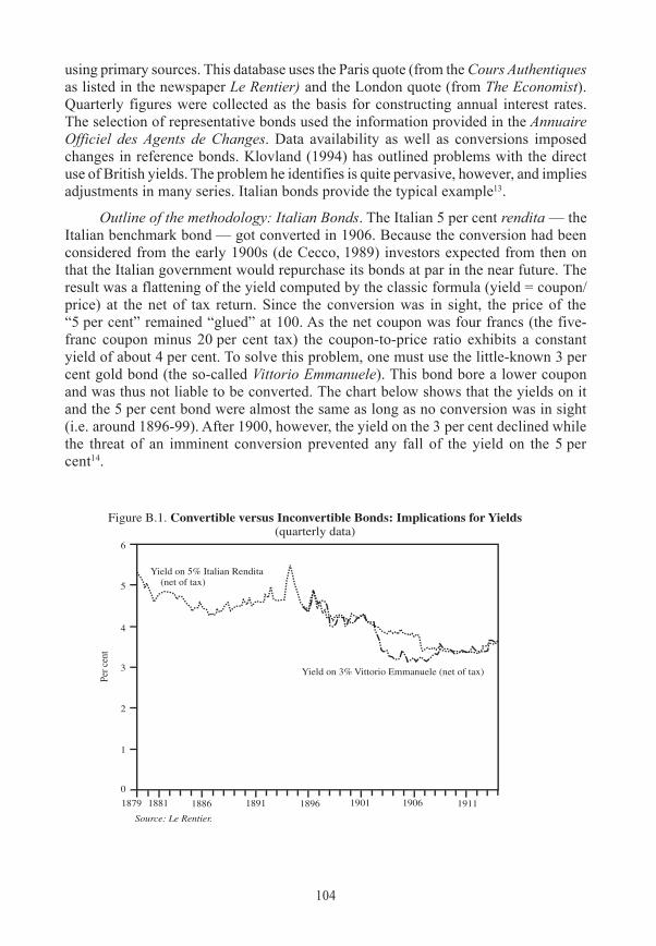
104

using primary sources. This database uses the Paris quote (from the Cours Authentiquesas listed in the newspaper Le Rentier) and the London quote (from The Economist).Quarterly figures were collected as the basis for constructing annual interest rates.The selection of representative bonds used the information provided in the AnnuaireOfficiel des Agents de Changes. Data availability as well as conversions imposedchanges in reference bonds. Klovland (1994) has outlined problems with the directuse of British yields. The problem he identifies is quite pervasive, however, and impliesadjustments in many series. Italian bonds provide the typical example13.

Outline of the methodology: Italian Bonds. The Italian 5 per cent rendita — theItalian benchmark bond — got converted in 1906. Because the conversion had beenconsidered from the early 1900s (de Cecco, 1989) investors expected from then onthat the Italian government would repurchase its bonds at par in the near future. Theresult was a flattening of the yield computed by the classic formula (yield = coupon/price) at the net of tax return. Since the conversion was in sight, the price of the“5 per cent” remained “glued” at 100. As the net coupon was four francs (the five-franc coupon minus 20 per cent tax) the coupon-to-price ratio exhibits a constantyield of about 4 per cent. To solve this problem, one must use the little-known 3 percent gold bond (the so-called Vittorio Emmanuele). This bond bore a lower couponand was thus not liable to be converted. The chart below shows that the yields on itand the 5 per cent bond were almost the same as long as no conversion was in sight(i.e. around 1896-99). After 1900, however, the yield on the 3 per cent declined whilethe threat of an imminent conversion prevented any fall of the yield on the 5 percent14.

105

Since the Rendita was more liquid, it is nonetheless preferable to work with itrather than with the Vittorio Emmanuele whenever possible. The conversion of 1906transformed the former 5 per cent into a bond that would now pay 4 per cent net oftaxes in 1906, 3.75 per cent net of tax until December 1911 and 3.5 per cent afterwards.One can compute the present value and solve for the yield in the post-conversionperiod. The result (shown in Figure B.1) is that the two bonds again imply virtuallyidentical yields, as arbitrage theory predicts. The series for Italian yields is thenconstructed (Figure B.2).

Series used. To minimise the type of problems discussed above, bonds werecarefully selected, as follows:

— Austria-Hungary: the 4 per cent gold Austrian bonds15;

— Argentina: the 1871 6 per cent until 1884:09; then the 5 per cent 1884 for1893:07-1897:07. The yield formula was adjusted for the Funding Loan, wherethere was a 60 per cent reduction of the coupon payments;

— Belgium, France, Germany and the Netherlands: yields from Homer and Sylla(1991);

— Brazil: the 5 per cent (gold) bonds until 1884:10, the 4.5 per cent 1883afterwards;

— Denmark: the 1893 3 per cent;

— Greece: before 1898, the 5 per cent (gold) 1881 and the 5 per cent (gold) 1884were combined. Between 1898 and 1904 the coupons on these bonds includedfixed rates plus potential bonuses depending on exchange-rate recovery. Theyield formula was computed assuming rational expectations on future exchange-rate changes. This way of computing provides a perfect adjustment on thesubsequent series, the new 1904 gold bond, which was actively traded afterwards;

106

— Italy: the 5 per cent Rendita (net of tax) until 1900:12, the 3 per cent (net of tax)until 1907:1 and the converted 5 per cent (reduced interest, non-taxable) afterwards;

— Norway: the 3.5 per cent 1886 and the 3 per cent 1888 are the two main series;

— Portugal: the 3 per cent consol. This bond was initially payable in gold, but themode of payment of the interest was modified in 1892 and 1902. Adjustmentwas made for the new coupon;

— Russia: the Emprunt 4 per cent 1867, known as Chemin de Fer Nicolas;

— Spain: until 1882, the 3 per cent exterior (gold), replaced in 1882 by a 4 percent gold consol ;

— Sweden: the 4 per cent 1880, the 4 per cent 1878, the 3 per cent 1888 and the3.5 per cent 1895 were combined;

— Switzerland: a combination of the 3 per cent 1890, the 3.5 per cent 1887 and the3 per cent 1897; and

— United Kingdom: yields from Klovland (1994).

Short-Term Interest Rates (Table DB.17)

The table reports average annual rates of discount of the central banks or maindiscount banks. The sources were:

— Austria-Hungary, Belgium, Denmark, Germany, Norway, Portugal, Russia, Spainand Sweden: Roulleau (1914);

— Argentina: from data communicated by Andres Regalsky;

— France: archives of the Bank of France;

— Greece: from data communicated by Olga Christodoulaki;

— Italy: de Mattia (1978) in Spinelli and Frattianni (1991), p. 85;

— Netherlands and Switzerland: Homer and Sylla (1991); and

— United Kingdom: The Economist.

Exchange Rates (Table DB.18)

For all countries except Greece, the exchange-rate series were constructed onthe basis of the monthly series in Schneider et al. (1991) and/or Schneider et al.(1997). The data are annual averages. The data for Greece come from an annual seriesreported in the archives of Crédit Lyonnais. For Argentina, Cortes Conde (1989) andDella Paolera (1988) also were used.

107

Exchange-Rate Volatility: An Index of Vulnerability (Table DB.19)

The formula used for exchange-rate volatility is intended to capture thevulnerability of public finances to an exchange-rate change. From this point of view,one needs to give more weight to exchange depreciation than to appreciation. Theresult is an asymmetric formula for annual vulnerability, computed on the basis ofmonthly exchange rates. It reads:

10x12

)/( 112

1 XXLnVol tt t � ¦

with

°¯

°®

­

�

!

�

��

�

0)/(0

0)/()/()/(

1

11

1

XXLnif

XXLnifXXLnXXLn

tt

tttt

tt

The monthly series used for the raw data are those listed above, except forGreece where an annual series is used in Table DB.18. Applying the formula forGreece relied on a monthly drachma-French franc series kindly communicated byOlga Christodoulaki.

Years on Gold (Table DB.20)

This table reproduces and enlarges the table provided in Flandreau et al. (1998)with a few corrections. As explained in the main text, the discussion of the exactbreakdown between years on gold and years off gold can be endless and is in any casenot very useful.

Part IV. Political Variables

Enfranchised Population (Table DB.21)

This table is constructed from the Polity Database16. Data are listed as the fractionof the population that is enfranchised, i.e. 0.5=50 per cent.

Political Events (Table DB.22)

The list provided focuses on main political and diplomatic events.

108

109

Database Tables

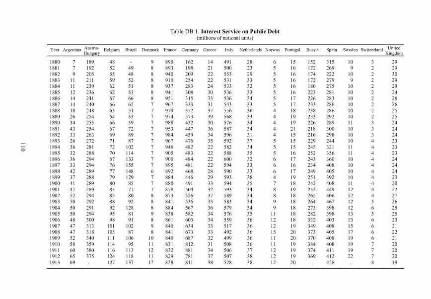
110

Table DB.1. Interest Service on Public Debt (millions of national units)

Year Argentina Austria-Hungary

Belgium Brazil Denmark France Germany Greece Italy Netherlands Norway Portugal Russia Spain Sweden Switzerland United Kingdom

1880 7 189 48 - 9 890 162 14 491 28 6 15 152 315 10 3 29 1881 7 192 52 49 8 893 198 21 500 23 5 16 172 269 9 2 29 1882 9 205 55 48 8 940 209 22 553 29 5 16 174 222 10 2 30 1883 11 211 59 52 8 910 254 22 531 33 5 16 172 279 9 2 29 1884 11 239 62 51 8 937 283 24 533 32 5 16 180 275 10 2 29 1885 12 236 62 53 8 941 308 30 536 33 5 16 223 281 10 2 24 1886 14 241 67 66 8 951 315 33 536 34 5 17 226 283 10 2 28 1887 14 240 66 62 7 967 333 31 543 33 5 17 233 286 10 2 26 1888 18 248 63 51 7 979 352 37 556 36 4 18 238 286 10 2 25 1889 26 254 64 53 7 974 373 39 568 33 4 19 233 292 10 2 25 1890 34 255 66 59 7 988 432 30 576 34 4 19 226 289 11 3 24 1891 43 254 67 72 7 953 447 36 587 34 4 21 218 300 10 3 24 1892 33 263 69 89 7 984 459 34 596 31 4 15 216 298 10 3 24 1893 26 272 71 87 7 967 476 35 592 37 5 15 229 244 10 4 23 1894 36 281 72 102 7 946 482 22 582 34 5 15 245 321 11 4 23 1895 32 288 70 114 7 905 483 22 588 35 5 16 252 356 11 4 23 1896 36 294 67 133 7 900 484 22 600 32 6 17 243 360 10 4 24 1897 33 294 76 155 7 895 481 22 594 33 6 16 234 408 10 4 24 1898 42 289 77 148 6 892 468 28 590 33 6 17 249 405 10 4 24 1899 37 288 79 129 7 884 446 29 593 38 4 19 251 392 10 4 23 1900 41 289 80 85 7 880 491 33 594 35 7 18 242 408 11 4 20 1901 47 289 83 77 7 878 504 32 593 34 8 19 252 449 12 4 22 1902 52 294 85 80 8 873 526 37 589 34 8 18 265 406 12 4 27 1903 50 292 88 92 8 841 536 33 583 34 9 18 264 467 12 5 26 1904 50 291 92 128 8 884 567 36 579 34 9 18 273 398 12 6 25 1905 50 294 95 81 9 838 582 34 576 35 11 18 282 398 13 5 25 1906 48 300 98 91 8 861 603 34 559 36 12 18 332 403 13 6 23 1907 47 313 101 102 9 840 634 33 517 36 12 19 349 408 15 6 21 1908 47 318 105 87 8 841 673 33 492 36 15 20 373 405 17 6 22 1909 52 340 111 106 10 840 687 32 499 36 11 20 370 408 19 6 21 1910 58 359 114 95 11 831 812 31 508 36 11 19 384 408 19 7 20 1911 60 380 116 113 12 832 881 34 506 37 12 19 374 411 19 7 20 1912 65 375 124 118 11 829 781 37 507 38 12 19 369 412 22 7 20 1913 69 - 127 137 12 828 811 38 528 38 12 20 - 458 - 8 19

111

Table DB.2. “Virtual” Service on Public Debt(millions of national units)

Argentina Brazil Greece Portugal Spain

1880 0 - 0 0 63 1881 0 0 0 0 106 1882 0 0 0 0 107 1883 0 0 0 0 0 1884 0 0 0 0 0 1885 0 0 0 0 0 1886 0 0 0 0 0 1887 0 0 0 0 0 1888 0 0 0 0 0 1889 0 0 0 0 0 1890 0 0 0 0 0 1891 11 0 0 0 0 1892 10 0 0 6 0 1893 16 0 23 8 0 1894 15 0 37 8 0 1895 16 0 38 7 0 1896 1 0 36 6 0 1897 3 0 35 8 0 1898 0 55 0 9 0 1899 0 51 0 7 0 1900 0 8 0 7 0 1901 0 0 0 7 0 1902 0 0 0 5 0 1903 0 0 0 0 0 1904 0 0 0 0 0 1905 0 0 0 0 0 1906 0 0 0 0 0 1907 0 0 0 0 0 1908 0 0 0 0 0 1909 0 0 0 0 0 1910 0 0 0 0 0 1911 0 0 0 0 0 1912 0 0 0 0 0 1913 0 0 0 0 0

112

Table DB.3. Percentage of Public Debt Serviced in Gold

Year Argentina Austria-Hungary

Belgium Brazil Denmark France Germany Greece Italy* Netherlands Norway Portugal Russia Spain Sweden Switzerland United Kingdom

1880 57 21 0 - 7 0 0 - 41 0 n.a. 43 - 47 n.a. n.a. 0 1881 67 23 0 45 7 0 0 - 33 0 n.a. 47 - 48 n.a. n.a. 0 1882 68 21 0 45 7 0 0 - 32 0 n.a. 46 - 61 n.a. n.a. 0 1883 64 22 0 48 7 0 0 - 29 0 n.a. 50 - 39 n.a. n.a. 0 1884 67 22 0 48 7 0 0 - 24 0 n.a. 55 45 43 n.a. n.a. 0 1885 51 21 0 50 7 0 0 43 28 0 n.a. 51 46 43 n.a. n.a. 0 1886 55 21 0 52 7 0 0 44 32 0 n.a. 54 48 43 n.a. n.a. 0 1887 76 24 0 46 7 0 0 64 33 0 n.a. 56 50 43 n.a. n.a. 0 1888 69 24 0 42 6 0 0 74 40 0 n.a. 56 50 43 n.a. n.a. 0 1889 50 24 0 45 6 0 0 74 39 n.a. 56 48 42 n.a. n.a. 0 1890 73 23 0 56 6 0 0 78 39 0 n.a. 61 45 41 n.a. n.a. 0 1891 98 23 0 75 6 0 0 79 48 0 n.a. 64 45 41 n.a. n.a. 0 1892 96 23 0 85 5 0 0 82 48 0 n.a. 33 49 38 n.a. n.a. 0 1893 97 25 0 82 5 0 0 61 50 0 n.a. 29 48 38 n.a. n.a. 0 1894 96 23 0 84 30 0 0 67 38 0 n.a. 28 49 37 n.a. n.a. 0 1895 91 24 0 83 33 0 0 69 29 0 n.a. 28 51 37 n.a. n.a. 0 1896 89 24 0 83 34 0 0 72 28 0 n.a. 31 53 33 n.a. n.a. 0 1897 89 24 0 83 66 0 0 70 27 0 n.a. 31 53 31 n.a. n.a. 0 1898 90 24 0 75 67 0 0 71 27 0 n.a. 29 53 23 n.a. n.a. 0 1899 79 23 0 75 67 0 0 72 25 0 n.a. 28 50 20 n.a. n.a. 0 1900 74 23 0 75 69 0 0 74 24 0 n.a. 27 50 15 n.a. n.a. 0 1901 83 22 0 70 72 0 0 76 22 0 n.a. 25 52 12 n.a. n.a. 0 1902 74 21 0 62 72 0 0 75 21 0 n.a. 40 53 11 n.a. n.a. 0 1903 78 20 0 90 72 0 0 77 17 0 n.a. 38 51 9 n.a. n.a. 0 1904 73 20 0 60 72 0 0 77 15 0 n.a. 34 51 9 n.a. n.a. 0 1905 69 20 0 85 72 0 0 75 14 0 n.a. 33 51 9 n.a. n.a. 0 1906 66 20 0 52 68 0 0 72 14 0 n.a. 32 57 9 n.a. n.a. 0 1907 63 19 0 74 66 0 0 67 12 0 n.a. 34 52 9 n.a. n.a. 0 1908 63 19 0 60 65 0 0 66 11 0 n.a. 32 51 9 n.a. n.a. 0 1909 64 19 0 59 73 0 0 67 12 0 n.a. 31 56 9 n.a. n.a. 0 1910 61 21 0 64 76 0 0 65 12 0 n.a. 30 55 11 n.a. n.a. 0 1911 64 21 0 55 77 0 0 62 12 0 n.a. 30 55 11 n.a. n.a. 0 1912 67 20 0 52 76 0 0 64 14 0 n.a. 31 56 11 n.a. n.a. 0 1913: 67 25 0 52 76 0 0 71 19 0 n.a. 30 56 11 n.a. n.a. 0

* Percentage serviced abroad.

113

Table DB.4. Government Revenue (millions of national units)

Year Argentina Austria-Hungary

Belgium Brazil Denmark France Germany Greece Italy Netherlands Norway Portugal Russia Spain Sweden Switzerland United Kingdom

1880 20 661 279 120 52 3531 1720 38 1236 116 - 26 732 792 - 43 82 1881 21 713 290 128 53 3785 1956 42 1321 111 40 28 738 787 101 43 84 1882 27 757 297 130 54 3644 2243 51 1354 116 43 30 791 780 100 44 87 1883 31 794 300 130 57 3653 2345 59 1336 112 41 29 751 802 104 50 86 1884 38 806 350 133 57 3449 2387 61 1299 133 45 31 758 793 104 48 88 1885 37 838 333 122 54 3320 2503 59 1410 116 44 32 776 816 106 48 90 1886 42 825 371 127 55 3169 2626 62 1447 123 43 35 792 887 104 61 91 1887 51 845 341 146 54 3244 3049 83 1431 119 45 38 843 803 97 60 90 1888 52 848 347 151 56 3268 3276 90 1442 124 45 39 903 852 110 60 90 1889 73 906 387 161 57 3271 3740 84 1507 125 51 39 948 800 116 61 95 1890 73 985 378 195 57 3376 3892 80 1576 166 52 41 969 740 122 68 97 1891 74 1025 402 229 57 3364 4083 86 1506 130 51 38 927 779 118 69 99 1892 110 1050 414 228 56 3370 3994 95 1447 132 53 43 1003 707 117 76 98 1893 123 1136 398 260 58 3366 4042 93 1448 127 54 46 1055 749 120 78 98 1894 121 1152 405 265 59 3458 4263 100 1466 133 55 49 1227 755 135 84 102 1895 132 1211 396 308 64 3416 4239 94 1518 132 59 52 1262 766 143 81 109 1896 124 1218 481 346 65 3436 4700 95 1535 134 66 50 1386 822 145 87 112 1897 151 1308 500 303 69 3528 4924 86 1527 136 77 49 1427 804 163 92 116 1898 136 1320 680 324 71 3620 5257 103 1548 144 85 51 1595 842 173 95 118 1899 166 1321 483 321 70 3657 5520 110 1566 148 67 54 1674 972 190 100 130 1900 151 1384 543 308 68 3815 5881 112 1589 155 88 55 1708 995 192 101 140 1901 151 1367 636 305 67 3634 6249 115 1620 153 90 53 1806 1023 185 102 153 1902 156 1403 628 344 77 3582 6205 114 1651 161 88 56 1910 1021 192 107 161 1903 172 1436 632 415 80 3668 6673 115 1675 166 90 58 2164 1039 228 113 151 1904 199 1489 529 443 98 3739 6261 116 1686 164 87 60 2021 1000 235 115 153 1905 212 1524 706 401 88 3766 6859 122 1772 176 95 61 2029 1010 245 130 154 1906 232 1634 676 432 107 3837 7301 126 1814 182 103 64 2279 1097 253 135 155 1907 246 1829 708 536 99 3968 7578 123 1797 184 111 71 2350 1080 282 147 157 1908 263 1927 699 441 93 3966 7769 123 1821 183 140 70 2430 1072 286 149 152 1909 285 2129 795 450 82 4141 8920 117 1917 191 120 73 2540 1066 290 157 132 1910 308 2275 815 525 91 4274 8820 130 2045 188 128 70 2805 1050 315 155 204 1911 316 2422 738 564 101 4689 9167 138 2152 206 138 66 2954 1131 398 99 185 1912 363 2526 778 615 124 4857 8961 131 2249 213 151 84 3108 1131 351 103 189 1913 370 - 808 654 125 5092 19768 129 2502 227 167 72 - 1505 - 101 198

114

Table DB.5. Government Revenue: Germany(millions of marks)

Year Federal Prussia Württemberg Baden Bavaria Saxony Hamburg Total Revenue

1880 530 799 38 34 225 65 30 1 721 1881 634 913 52 39 222 65 31 1 956 1882 602 1 214 52 41 229 72 34 2 243 1883 567 1 297 3 41 277 72 35 2 292 1884 594 1 350 54 41 242 71 36 2 387 1885 615 1 442 54 42 242 71 38 2 503 1886 672 1 474 55 43 241 102 38 2 626 1887 949 1 614 56 45 241 102 40 3 049 1888 996 1 741 56 48 282 112 42 3 276 1889 1 206 1 960 60 48 306 112 47 3 740 1890 1 253 2 061 61 62 280 124 52 3 892 1891 1 414 2 078 65 66 280 124 55 4 083 1892 1 137 2 209 66 69 306 149 58 3 994 1893 1 290 2 101 65 70 306 149 61 4 042 1894 1 344 2 241 67 76 328 143 64 4 263 1895 1 294 2 261 71 77 328 143 66 4 239 1896 1 655 2 326 71 79 345 151 72 4 700 1897 1 733 2 466 74 82 345 151 73 4 924 1898 1 857 2 596 75 84 379 189 77 5 257 1899 1 973 2 726 81 86 379 189 84 5 520 1900 2 097 2 885 82 89 433 205 89 5 881 1901 2 416 2 919 90 91 433 205 96 6 249 1902 2 177 3 059 91 100 455 223 101 6 205 1903 2 442 3 256 90 99 455 223 109 6 673 1904 2 071 3 269 91 95 442 207 109 6 284 1905 2 473 3 400 83 161 442 207 120 6 886 1906 2 455 3 867 84 171 484 166 108 7 334 1907 2 601 4 054 91 99 484 166 118 7 612 1908 2 540 4 151 92 112 566 187 154 7 804 1909 3 416 4 408 100 116 564 187 177 8 969 1910 3 041 4 530 104 129 647 218 200 8 869 1911 3 012 4 903 108 115 647 218 207 9 209 1912 3 496 4 085 112 112 720 267 222 9 015 1913 14 253 4 241 119 115 720 267 226 19 942 1914 13 806 5 505 122 115 745 199 186 20 678

115

Table DB.6. Deficits (millions of national units; a positive number is a surplus)

Year Argentina Austria-Hungary

Belgium Brazil Denmark France Germany Greece Italy Netherlands Norway Portugal Russia Spain Sweden Switzerland United Kingdom

1880 -13 -93 5 -30 -22 166 -23 -50 21 2 - -8 -81 -58 - 1 1 1881 -9 -270 3 -11 4 169 20 -60 43 -12 -8 -6 -97 -1 4 1 1 1882 -31 -76 -14 -9 3 -43 72 -6 -19 -13 -5 -2 38 -31 8 0 0 1883 -14 -50 -25 -23 6 -62 98 -9 -52 -26 -1 -6 -20 -45 4 0 1 1884 -18 -467 -12 -21 10 -90 43 -31 -77 0 -1 -8 -13 -28 5 1 -1 1885 -19 -40 -18 -36 4 -147 39 -63 -48 -6 0 -10 -47 -82 3 2 -3 1886 -12 -29 22 -27 -3 -125 43 -68 -98 -1 -1 -9 -50 -15 -11 3 1 1887 -14 -78 -5 -5 -6 -17 170 -24 -246 -4 -1 -4 10 -73 -10 7 3 1888 -24 -70 -9 4 -4 47 129 -19 -391 -3 -2 -14 67 -122 -12 1 3 1889 -34 -114 14 -25 -5 24 264 -85 -277 0 -1 -13 91 -67 10 0 4 1890 -22 -19 -39 -26 -9 91 29 -62 -87 -1 -2 -14 1 -50 10 1 3 1891 -63 -312 0 8 -8 106 266 -37 -93 -1 -3 -15 -64 -54 -1 -4 3 1892 -27 -64 8 -51 -7 -10 -57 -13 -78 -20 -8 -6 -87 -19 -6 -10 2 1893 -7 -100 3 -41 -4 -85 102 1 -94 -9 -10 0 50 75 -3 -8 0 1894 -22 -91 3 -108 -3 -22 107 15 -108 1 -9 -1 121 6 0 0 1 1895 -35 30 -15 -37 -2 -18 118 2 -74 -1 -14 -1 54 -26 23 5 4 1896 -106 3 43 -23 -1 -9 169 4 -51 1 -14 -11 111 40 16 8 3 1897 -28 8 -12 -76 -7 4 111 -51 -6 -6 -6 -7 32 -54 26 4 4 1898 -175 -14 -14 -456 -5 92 134 -209 21 -6 -14 -4 4 8 31 1 0 1899 -8 -7 -87 -67 -7 68 190 5 30 -2 -14 -6 74 134 -2 2 -14 1900 -8 -4 -31 -173 -11 68 87 2 43 1 -22 -3 -40 52 -9 -2 -53 1901 -12 -49 32 -66 -10 -122 288 1 57 0 -16 -6 16 38 -13 -4 -53 1902 -47 -68 12 46 -1 -117 26 -10 71 -2 -17 -4 -199 71 -7 1 -33 1903 -11 -92 4 52 0 71 302 -1 70 1 -12 -8 124 23 16 2 -4 1904 4 -105 0 -20 -2 100 150 0 63 -12 -8 -2 -680 54 -25 0 4 1905 -110 -76 80 26 3 59 469 6 -177 2 -6 -6 -974 72 16 13 7 1906 -38 -6 -97 9 -7 -15 307 4 -245 3 -7 -4 -404 103 -36 5 11 1907 -7 -328 -60 14 5 88 -60 -9 -80 1 2 -6 -116 65 -32 -1 13 1908 11 -152 -71 -70 -15 -55 -49 -11 -156 -11 -1 -5 -125 56 -61 -4 7 1909 -107 -701 9 -68 -46 -45 47 -20 -194 -6 -7 -8 -24 -51 -11 -28 -25 1910 -103 -56 -14 -99 -33 -48 -94 -11 -175 -19 4 -2 261 -6 15 -5 36 1911 -101 4 -73 -118 -21 141 29 -43 -341 -3 -1 -7 213 6 3 0 11 1912 -41 -105 -118 -174 3 114 -136 -77 -615 -11 -15 0 136 -62 -99 1 5 1913 -33 - -121 -109 2 25 4 -133 -357 -11 -17 -3 - -71 - -5 6

116

Table DB.7. Nominal Public Debt (millions of national units)

Year Argentina Austria-Hungary

Belgium Brazil Denmark France Germany Greece Italy Netherlands Norway Portugal Russia Spain Sweden Switzerland United Kingdom

1880 104 4 613 1 423 614 203 24 279 4 292 - 9 999 942 114 376 5 500 13 741 222 34 765 1881 116 4 974 1 439 611 202 25 303 5 158 - 10 774 941 115 407 5 780 13 586 227 35 760 1882 124 5 181 1 554 615 201 25 102 5 451 - 12 028 999 114 413 5 600 11 221 225 37 754 1883 128 5 272 1 763 647 200 26 418 5 917 - 12 133 1 004 112 448 5 700 7 454 229 34 746 1884 125 5 455 1 767 652 198 27 354 6 642 315 11 559 1 019 114 489 5 191 6 908 231 33 740 1885 157 5 554 1 772 678 195 28 255 7 290 281 11 626 1 081 113 513 5 070 6 877 247 36 742 1886 163 5 670 1 902 706 196 28 741 7 481 284 11 646 1 079 117 511 5 159 6 867 247 37 736 1887 192 5 993 1 916 708 194 29 433 7 656 441 11 680 1 098 115 547 5 663 6 823 246 34 705 1888 411 5 959 1 928 662 191 29 892 8 137 618 12 157 1 095 126 569 5 545 6 787 268 31 698 1889 527 6 127 1 973 693 189 30 055 8 327 616 12 612 1 093 124 576 5 290 6 883 262 55 689 1890 932 6 358 2 003 869 187 30 096 92 90 738 12 640 1 089 126 630 5 097 6 887 262 71 684 1891 1 386 6 698 2 062 1 087 186 30 481 10 154 816 12 945 1 112 135 720 5 298 6 920 267 61 677 1892 1 401 6 702 2 128 1 702 184 30 612 10 748 849 13 150 1 106 135 704 5 696 7 176 276 64 671 1893 1 390 6 893 2 170 1 488 183 31 035 11 083 969 13 179 1 122 174 712 5 916 7 228 281 65 667 1894 1 413 6 861 2 205 1 673 209 31 065 11 445 1 088 13 038 1 116 155 706 6 592 7 284 295 85 659 1895 1 384 6 952 2 227 2 103 200 31 094 11 628 1 152 13 275 1 104 171 719 6 615 7 400 290 84 652 1896 1 246 6 848 2 309 2 100 197 30 235 11 808 1 190 13 414 1 111 195 800 6 735 7 977 291 81 645 1897 1 276 6 860 2 370 2 192 209 30 100 11 920 1 143 13 409 1 095 195 840 6 341 8 378 289 84 639 1898 1 171 6 862 2 604 1 975 206 29 948 11 984 1 099 13 676 1 107 213 794 6 165 10 596 285 84 635 1899 1 235 6 943 2 607 1 956 208 30 055 12 260 1 140 13 712 1 149 241 801 6 225 11 449 319 90 639 1900 1 033 7 227 2 651 1 701 218 30 097 12 388 1 207 13 921 1 145 243 805 6 211 12 729 339 92 704 1901 1 032 7 210 2 778 1 801 247 30 344 12 888 1 264 13 911 1 159 276 771 6 431 13 363 351 88 765 1902 988 7 218 2 879 1 822 245 30 346 13 542 1 266 13 803 1 140 275 647 6 644 13 337 348 90 798 1903 968 7 233 2 989 1 935 243 30 375 13 813 1 274 13 684 1 152 283 659 6 636 12 744 347 119 795 1904 968 7 328 3 117 1 888 242 30 460 14 329 1 219 13 919 1 133 322 631 7 066 12 638 386 102 797 1905 873 7 388 3 221 1 640 240 30 702 14 532 1 099 13 978 1 106 359 643 7 841 12 523 383 103 789 1906 862 7 485 3 286 1 611 252 30 348 15 108 979 14 361 1 145 353 642 8 626 12 533 423 101 779 1907 950 7 676 3 365 1 689 256 30 162 16 066 874 14 613 1 140 348 675 8 725 12 475 464 99 762 1908 906 7 724 3 437 1 767 254 30 375 16 629 849 14 726 1 134 347 665 8 851 12 390 515 102 754 1909 1 021 7 744 3 581 1 802 302 32 864 18 501 840 14 946 1 128 351 661 9 039 12 471 526 126 763 1910 1 028 9 026 3 703 1 915 336 32 558 19 416 792 15 157 1 122 386 669 9 030 10 480 537 123 733 1911 1 195 9 153 3 734 1 967 352 32 720 19 577 759 15 545 1 117 384 684 8 958 10 420 537 120 718 1912 1 207 9 335 3 739 1 952 357 32 881 19 605 829 15 467 1 163 381 687 8 858 10 350 606 118 711 1913 1 237 9 516 3 743 2 147 358 32 889 20 189 959 16 382 1 156 366 - 9 888 10 372 602 117 706

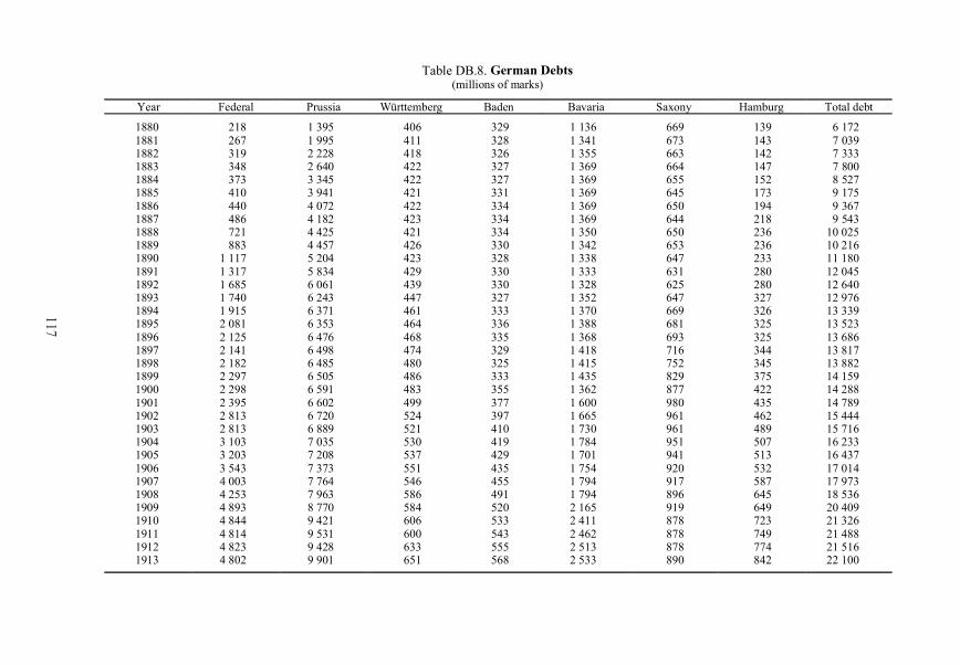
117

Table DB.8. German Debts(millions of marks)

Year Federal Prussia Württemberg Baden Bavaria Saxony Hamburg Total debt

1880 218 1 395 406 329 1 136 669 139 6 1721881 267 1 995 411 328 1 341 673 143 7 0391882 319 2 228 418 326 1 355 663 142 7 3331883 348 2 640 422 327 1 369 664 147 7 8001884 373 3 345 422 327 1 369 655 152 8 5271885 410 3 941 421 331 1 369 645 173 9 1751886 440 4 072 422 334 1 369 650 194 9 3671887 486 4 182 423 334 1 369 644 218 9 5431888 721 4 425 421 334 1 350 650 236 10 0251889 883 4 457 426 330 1 342 653 236 10 2161890 1 117 5 204 423 328 1 338 647 233 11 1801891 1 317 5 834 429 330 1 333 631 280 12 0451892 1 685 6 061 439 330 1 328 625 280 12 6401893 1 740 6 243 447 327 1 352 647 327 12 9761894 1 915 6 371 461 333 1 370 669 326 13 3391895 2 081 6 353 464 336 1 388 681 325 13 5231896 2 125 6 476 468 335 1 368 693 325 13 6861897 2 141 6 498 474 329 1 418 716 344 13 8171898 2 182 6 485 480 325 1 415 752 345 13 8821899 2 297 6 505 486 333 1 435 829 375 14 1591900 2 298 6 591 483 355 1 362 877 422 14 2881901 2 395 6 602 499 377 1 600 980 435 14 7891902 2 813 6 720 524 397 1 665 961 462 15 4441903 2 813 6 889 521 410 1 730 961 489 15 7161904 3 103 7 035 530 419 1 784 951 507 16 2331905 3 203 7 208 537 429 1 701 941 513 16 4371906 3 543 7 373 551 435 1 754 920 532 17 0141907 4 003 7 764 546 455 1 794 917 587 17 9731908 4 253 7 963 586 491 1 794 896 645 18 5361909 4 893 8 770 584 520 2 165 919 649 20 4091910 4 844 9 421 606 533 2 411 878 723 21 3261911 4 814 9 531 600 543 2 462 878 749 21 4881912 4 823 9 428 633 555 2 513 878 774 21 5161913 4 802 9 901 651 568 2 533 890 842 22 100

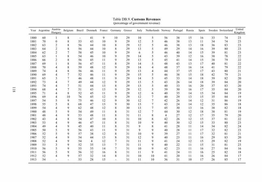
118

Table DB.9. Customs Revenues (percentage of government revenue)

Year Argentina Austria-Hungary

Belgium Brazil Denmark France Germany Greece Italy Netherlands Norway Portugal Russia Spain Sweden Switzerland United Kingdom

1880 60 1 8 - 41 9 10 29 10 5 56 38 15 16 33 74 23 1881 70 0 8 53 43 10 9 29 12 5 46 38 13 11 34 74 23 1882 63 2 8 56 44 10 8 29 12 5 46 38 13 18 36 83 23 1883 64 2 8 56 44 10 8 29 13 5 49 29 14 16 39 80 23 1884 62 2 7 58 45 10 9 29 6 5 46 40 14 15 39 81 23 1885 63 1 8 54 46 10 9 29 14 5 43 39 12 16 38 78 22 1886 66 2 8 56 45 11 9 29 13 5 45 41 14 15 38 79 22 1887 69 1 8 56 47 11 8 29 14 5 48 43 13 17 40 81 22 1888 70 4 8 59 48 12 9 29 14 4 48 37 16 14 41 79 22 1889 74 4 8 56 46 11 9 29 13 4 44 37 15 17 43 80 21 1890 69 4 7 52 46 11 9 29 15 5 46 38 15 18 42 79 21 1891 65 3 7 46 48 11 9 29 14 5 45 33 14 18 39 82 20 1892 73 4 7 49 44 12 9 29 13 5 43 26 14 18 39 84 20 1893 74 4 7 51 44 13 8 29 13 5 40 33 16 20 37 83 20 1894 68 4 7 51 43 13 9 29 12 5 39 30 16 17 35 84 20 1895 71 4 8 52 45 11 9 29 12 6 40 35 14 15 34 84 19 1896 69 4 10 76 45 12 9 29 12 7 40 29 13 15 35 84 19 1897 54 5 9 75 46 12 9 30 12 7 42 26 14 12 31 86 19 1898 55 5 8 68 47 13 9 30 13 7 43 24 14 12 35 86 18 1899 54 4 9 62 48 12 8 30 13 7 45 30 13 16 38 82 18 1900 48 5 9 54 49 11 8 31 12 7 44 30 12 18 38 81 19 1901 48 4 9 53 48 11 8 31 11 8 4 27 12 17 35 79 20 1902 43 4 8 54 47 10 8 31 10 8 42 26 12 15 37 81 22 1903 53 4 9 46 47 11 8 31 10 9 40 30 12 15 33 80 23 1904 49 4 9 45 40 11 8 31 9 8 41 28 11 14 34 82 24 1905 50 5 9 56 43 11 9 31 9 9 40 28 11 17 32 82 23 1906 52 5 9 57 38 12 8 31 10 9 39 27 11 17 32 81 21 1907 52 4 9 54 44 13 8 31 12 9 40 23 11 16 29 83 20 1908 52 4 9 54 4 12 7 31 11 9 41 24 12 15 29 82 19 1909 53 3 9 52 35 13 7 31 11 9 40 22 11 15 31 81 23 1910 56 5 9 55 35 14 7 31 10 9 42 23 11 16 27 84 16 1911 56 5 9 56 32 16 8 31 11 9 41 24 11 16 25 82 18 1912 52 4 9 57 32 14 8 31 10 10 41 20 11 16 26 84 17 1913 54 - - 53 28 15 - 31 11 10 36 31 10 17 26 85 17

119

Table DB.10. Central Bank Reserves(millions of national units)

Year Argentina Austria-Hungary

Belgium Brazil Denmark France Germany Greece Italy Netherlands Norway Portugal Russia Spain Sweden Switzerland United Kingdom

1880 3 187 154 9 43 1 787 539 21 178 140 34 2 176 236 28 - 24 1881 6 200 140 7 48 1 817 531 13 138 107 30 3 172 226 26 - 20 1882 8 193 154 6 45 2 056 566 13 159 97 33 2 171 125 19 - 20 1883 14 199 168 6 45 1 963 576 14 320 116 35 2 198 111 20 57 22 1884 7 206 176 7 45 2 049 538 18 371 120 34 2 202 168 25 64 21 1885 7 209 183 7 44 2 243 634 26 337 142 29 2 273 152 23 66 20 1886 26 217 178 6 45 2 385 688 9 345 175 30 3 283 238 27 67 19 1887 2 224 170 5 48 2 310 781 9 378 148 40 4 251 310 24 76 20 1888 7 233 150 9 50 2 251 863 10 435 152 45 6 273 222 29 74 19 1889 2 241 176 10 48 2 521 776 12 437 134 47 5 308 129 27 76 18 1890 2 244 178 12 50 2 372 782 8 409 105 39 4 416 89 22 81 23 1891 0 245 195 28 52 2 592 925 12 442 120 35 4 450 127 24 85 22 1892 2 289 209 22 52 2 979 861 10 447 124 39 7 534 139 27 89 24 1893 3 278 209 19 54 2 974 832 9 446 130 32 9 407 183 28 89 25 1894 3 307 230 34 54 3 312 1 047 9 510 133 33 11 416 285 38 92 33 1895 3 377 209 40 57 3 185 898 9 502 127 37 12 512 266 39 94 44 1896 2 448 204 31 60 3 143 855 9 511 114 35 13 668 260 40 96 34 1897 2 505 223 24 60 3 159 888 14 461 165 48 13 1 159 266 39 100 30 1898 2 490 212 26 59 3 030 814 11 476 84 44 14 999 200 44 104 29 1899 4 509 217 22 65 3 031 743 15 466 118 43 14 876 367 42 107 29 1900 2 609 245 21 67 3 447 806 17 457 127 36 13 734 395 43 109 29 1901 2 724 279 29 65 3 567 936 17 472 144 40 12 701 369 64 117 32 1902 0 733 284 42 64 3 650 869 21 491 136 34 11 765 394 70 114 29 1903 88 731 272 45 69 3 462 878 22 662 128 31 12 908 410 73 119 28 1904 126 754 283 61 75 3 761 1 014 28 687 142 37 11 978 419 74 131 30 1905 231 713 253 58 78 3 953 887 35 845 154 38 12 1 135 437 87 143 29 1906 271 727 269 25 84 3 704 736 41 974 137 46 11 1 144 455 95 155 29 1907 283 720 284 47 90 3 615 701 46 1 132 150 48 10 1 187 454 93 168 31 1908 344 768 344 60 77 4 371 1 059 45 1 151 152 48 9 1 193 458 94 180 31 1909 456 857 308 41 74 4 371 984 49 1 174 157 50 12 1 379 491 105 192 33 1910 490 835 377 53 73 4 106 1 002 91 1 198 150 55 11 1 376 505 107 204 33 1911 497 818 396 48 72 4 011 1 057 132 1 247 150 60 13 1 381 512 117 229 32 1912 574 754 437 35 73 3 896 1 038 216 1 287 170 62 16 1 513 592 123 216 30 1913 597 784 472 38 77 4 158 1 476 230 1 355 160 74 16 1 616 650 102 243 33

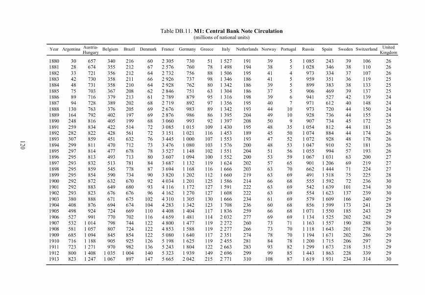
120

Table DB.11. M1: Central Bank Note Circulation (millions of national units)

Year Argentina Austria-Hungary

Belgium Brazil Denmark France Germany Greece Italy Netherlands Norway Portugal Russia Spain Sweden Switzerland United Kingdom

1880 30 657 340 216 60 2 305 730 51 1 527 191 39 5 1 085 243 39 106 26 1881 28 674 355 212 67 2 576 760 78 1 498 194 38 5 1 028 346 38 110 26 1882 33 721 356 212 64 2 732 756 88 1 506 195 41 4 973 334 37 107 26 1883 42 730 358 211 66 2 926 737 98 1 346 186 41 5 959 351 36 119 25 1884 48 731 358 210 64 2 928 762 80 1 342 186 39 5 899 383 38 133 25 1885 75 703 367 208 62 2 846 751 63 1 304 186 37 5 906 469 39 137 25 1886 89 716 379 213 61 2 789 879 95 1 316 198 39 6 941 527 42 139 24 1887 94 728 389 202 68 2 719 892 97 1 356 195 40 7 971 612 40 148 24 1888 130 763 376 205 69 2 676 983 89 1 342 193 44 10 973 720 44 150 24 1889 164 792 402 197 69 2 876 986 86 1 395 204 49 10 928 736 44 155 24 1890 248 816 405 199 68 3 060 993 92 1 397 208 50 9 907 734 45 172 25 1891 259 834 422 514 72 3 085 1 015 109 1 430 195 48 35 1 054 812 44 181 26 1892 282 822 428 561 72 3 151 1 021 116 1 453 189 45 50 1 074 884 44 174 26 1893 307 859 451 632 76 3 445 1 000 107 1 553 193 47 52 1 072 928 48 178 26 1894 299 811 470 712 73 3 476 1 080 103 1 576 200 48 53 1 047 910 52 181 26 1895 297 814 477 678 78 3 527 1 148 102 1 551 204 51 56 1 055 994 57 193 26 1896 295 813 493 713 80 3 607 1 094 100 1 552 200 53 59 1 067 1 031 63 200 27 1897 293 832 513 781 84 3 687 1 132 119 1 624 202 57 65 901 1 206 69 219 27 1898 295 859 545 778 87 3 694 1 168 116 1 666 203 63 70 662 1 444 71 224 27 1899 295 854 590 734 90 3 820 1 202 112 1 660 219 63 69 491 1 518 75 225 28 1900 292 872 632 670 92 4 034 1 201 125 1 586 214 66 68 555 1 592 72 236 30 1901 292 883 649 680 93 4 116 1 172 127 1 591 222 63 69 542 1 639 101 234 30 1902 293 823 676 676 96 4 162 1 270 127 1 608 222 63 69 554 1 623 137 239 30 1903 380 888 671 675 102 4 310 1 305 130 1 666 234 61 69 579 1 609 166 240 29 1904 408 876 694 674 104 4 283 1 342 123 1 708 236 60 68 856 1 599 173 241 28 1905 498 924 724 669 110 4 408 1 404 117 1 836 259 66 68 1 071 1 550 185 243 29 1906 527 991 770 702 116 4 659 1 481 114 2 032 277 69 69 1 134 1 525 202 242 29 1907 532 1 014 798 744 122 4 800 1 477 119 2 272 260 73 71 1 163 1 557 190 288 29 1908 581 1 057 807 724 122 4 853 1 588 119 2 277 266 73 70 1 118 1 643 201 278 30 1909 685 1 094 845 854 122 5 080 1 640 117 2 351 274 78 70 1 194 1 671 202 286 29 1910 716 1 188 905 925 126 5 198 1 625 119 2 455 281 84 78 1 200 1 715 206 297 29 1911 723 1 271 970 982 136 5 243 1 804 122 2 663 283 93 82 1 299 1 673 218 315 29 1912 800 1 408 1 035 1 004 140 5 323 1 939 149 2 696 299 99 85 1 443 1 863 228 339 29 1913 823 1 247 1 067 897 147 5 665 2 042 215 2 771 310 108 87 1 619 1 931 234 314 30

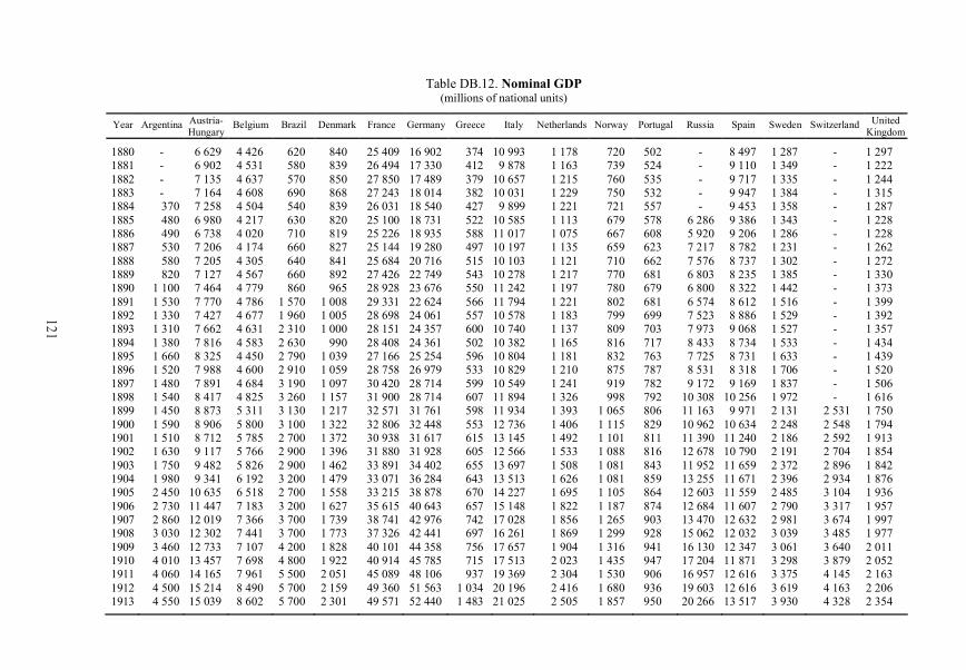
121

Table DB.12. Nominal GDP (millions of national units)

Year Argentina Austria-Hungary

Belgium Brazil Denmark France Germany Greece Italy Netherlands Norway Portugal Russia Spain Sweden Switzerland United Kingdom

1880 - 6 629 4 426 620 840 25 409 16 902 374 10 993 1 178 720 502 - 8 497 1 287 - 1 297 1881 - 6 902 4 531 580 839 26 494 17 330 412 9 878 1 163 739 524 - 9 110 1 349 - 1 222 1882 - 7 135 4 637 570 850 27 850 17 489 379 10 657 1 215 760 535 - 9 717 1 335 - 1 244 1883 - 7 164 4 608 690 868 27 243 18 014 382 10 031 1 229 750 532 - 9 947 1 384 - 1 315 1884 370 7 258 4 504 540 839 26 031 18 540 427 9 899 1 221 721 557 - 9 453 1 358 - 1 287 1885 480 6 980 4 217 630 820 25 100 18 731 522 10 585 1 113 679 578 6 286 9 386 1 343 - 1 228 1886 490 6 738 4 020 710 819 25 226 18 935 588 11 017 1 075 667 608 5 920 9 206 1 286 - 1 228 1887 530 7 206 4 174 660 827 25 144 19 280 497 10 197 1 135 659 623 7 217 8 782 1 231 - 1 262 1888 580 7 205 4 305 640 841 25 684 20 716 515 10 103 1 121 710 662 7 576 8 737 1 302 - 1 272 1889 820 7 127 4 567 660 892 27 426 22 749 543 10 278 1 217 770 681 6 803 8 235 1 385 - 1 330 1890 1 100 7 464 4 779 860 965 28 928 23 676 550 11 242 1 197 780 679 6 800 8 322 1 442 - 1 373 1891 1 530 7 770 4 786 1 570 1 008 29 331 22 624 566 11 794 1 221 802 681 6 574 8 612 1 516 - 1 399 1892 1 330 7 427 4 677 1 960 1 005 28 698 24 061 557 10 578 1 183 799 699 7 523 8 886 1 529 - 1 392 1893 1 310 7 662 4 631 2 310 1 000 28 151 24 357 600 10 740 1 137 809 703 7 973 9 068 1 527 - 1 357 1894 1 380 7 816 4 583 2 630 990 28 408 24 361 502 10 382 1 165 816 717 8 433 8 734 1 533 - 1 434 1895 1 660 8 325 4 450 2 790 1 039 27 166 25 254 596 10 804 1 181 832 763 7 725 8 731 1 633 - 1 439 1896 1 520 7 988 4 600 2 910 1 059 28 758 26 979 533 10 829 1 210 875 787 8 531 8 318 1 706 - 1 520 1897 1 480 7 891 4 684 3 190 1 097 30 420 28 714 599 10 549 1 241 919 782 9 172 9 169 1 837 - 1 506 1898 1 540 8 417 4 825 3 260 1 157 31 900 28 714 607 11 894 1 326 998 792 10 308 10 256 1 972 - 1 616 1899 1 450 8 873 5 311 3 130 1 217 32 571 31 761 598 11 934 1 393 1 065 806 11 163 9 971 2 131 2 531 1 750 1900 1 590 8 906 5 800 3 100 1 322 32 806 32 448 553 12 736 1 406 1 115 829 10 962 10 634 2 248 2 548 1 794 1901 1 510 8 712 5 785 2 700 1 372 30 938 31 617 615 13 145 1 492 1 101 811 11 390 11 240 2 186 2 592 1 913 1902 1 630 9 117 5 766 2 900 1 396 31 880 31 928 605 12 566 1 533 1 088 816 12 678 10 790 2 191 2 704 1 854 1903 1 750 9 482 5 826 2 900 1 462 33 891 34 402 655 13 697 1 508 1 081 843 11 952 11 659 2 372 2 896 1 842 1904 1 980 9 341 6 192 3 200 1 479 33 071 36 284 643 13 513 1 626 1 081 859 13 255 11 671 2 396 2 934 1 876 1905 2 450 10 635 6 518 2 700 1 558 33 215 38 878 670 14 227 1 695 1 105 864 12 603 11 559 2 485 3 104 1 936 1906 2 730 11 447 7 183 3 200 1 627 35 615 40 643 657 15 148 1 822 1 187 874 12 684 11 607 2 790 3 317 1 957 1907 2 860 12 019 7 366 3 700 1 739 38 741 42 976 742 17 028 1 856 1 265 903 13 470 12 632 2 981 3 674 1 997 1908 3 030 12 302 7 441 3 700 1 773 37 326 42 441 697 16 261 1 869 1 299 928 15 062 12 032 3 039 3 485 1 977 1909 3 460 12 733 7 107 4 200 1 828 40 101 44 358 756 17 657 1 904 1 316 941 16 130 12 347 3 061 3 640 2 011 1910 4 010 13 457 7 698 4 800 1 922 40 914 45 785 715 17 513 2 023 1 435 947 17 204 11 871 3 298 3 879 2 052 1911 4 060 14 165 7 961 5 500 2 051 45 089 48 106 937 19 369 2 304 1 530 906 16 957 12 616 3 375 4 145 2 163 1912 4 500 15 214 8 490 5 700 2 159 49 360 51 563 1 034 20 196 2 416 1 680 936 19 603 12 616 3 619 4 163 2 206 1913 4 550 15 039 8 602 5 700 2 301 49 571 52 440 1 483 21 025 2 505 1 857 950 20 266 13 517 3 930 4 328 2 354

122

Tabl

e D

B.1

3. P

rice

s

Yea

r A

rgen

tina

Aus

tria-

Hun

gary

Be

lgiu

m

Braz

il D

enm

ark

Fran

ce

Ger

man

y G

reec

e Ita

ly

Net

herla

nds

Nor

way

Po

rtuga

l Ru

ssia

Sp

ain

Swed

en

Switz

erla

nd

Uni

ted

Kin

gdom

1880

-

88.0

0 98

.00

36.2

6 10

8.60

98

.40

87.0

0 73

.16

93.3

0 94

.70

81.4

0 82

.18

- 90

.00

91.0

0 10

2.40

11

1.00

18

81

- 86

.80

99.0

0 33

.92

107.

60

97.8

0 85

.00

70.8

4 87

.26

94.6

0 82

.30

84.1

6 -

90.6

0 89

.00

96.9

2 10

9.00

18

82

- 87

.60

98.0

0 37

.50

104.

00

96.0

0 81

.00

93.0

3 89

.56

95.7

0 82

.80

85.1

5 -

93.9

0 88

.00

98.5

6 11

0.00

18

83

- 86

.70

96.0

0 48

.42

102.

80

99.0

0 80

.00

95.6

3 83

.91

92.0

0 81

.40

81.1

9 -

89.5

0 85

.00

92.7

9 10

8.00

18

84

34.3

0 84

.50

93.0

0 37

.89

98.9

0 97

.10

78.0

0 95

.46

80.3

6 90

.70

78.1

0 76

.24

- 81

.50

82.0

0 88

.65

98.0

0 18

85

41.9

6 80

.50

86.0

0 41

.45

97.1

0 94

.70

75.0

0 83

.38

84.6

7 88

.50

73.5

0 74

.26

79.5

3 80

.50

78.0

0 83

.46

92.0

0 18

86

42.8

5 79

.00

81.0

0 39

.34

93.7

0 93

.30

72.0

0 75

.35

85.1

5 87

.40

72.1

0 75

.25

76.5

6 79

.90

75.0

0 83

.08

87.0

0 18

87

41.3

9 76

.90

81.0

0 33

.08

91.8

0 90

.70

73.0

0 98

.42

76.4

1 89

.10

70.2

0 74

.26

78.3

6 77

.00

72.0

0 83

.94

85.0

0 18

88

41.2

1 76

.80

83.0

0 32

.08

91.1

0 91

.70

75.0

0 95

.18

80.7

5 89

.70

71.6

0 74

.26

84.0

7 78

.40

79.0

0 82

.02

87.0

0 18

89

49.7

0 78

.30

84.0

0 31

.58

92.7

0 91

.90

82.0

0 99

.09

85.4

4 89

.50

74.0

0 79

.21

79.7

8 79

.70

79.0

0 86

.83

89.0

0 18

90

69.6

7 78

.50

86.0

0 41

.15

95.1

0 91

.10

86.5

0 95

.93

87.6

4 92

.40

74.0

0 87

.13

79.3

3 79

.10

82.0

0 87

.98

89.0

0 18

91

108.

92

80.4

0 86

.00

75.1

2 97

.40

92.7

0 86

.00

99.0

6 85

.25

92.0

0 77

.20

85.1

5 83

.04

78.0

0 82

.00

85.8

7 92

.00

1892

86

.99

77.8

0 82

.00

98.2

5 96

.10

91.9

0 80

.00

99.8

7 81

.03

88.4

0 75

.80

87.1

3 86

.09

80.2

0 77

.00

81.9

2 87

.00

1893

81

.62

77.5

0 80

.00

110.

53

93.7

0 90

.40

77.0

0 11

0.70

75

.96

89.2

0 74

.40

88.1

2 79

.18

78.1

0 74

.00

81.5

4 85

.00

1894

79

.85

77.1

0 78

.00

131.

83

90.9

0 93

.30

73.0

0 10

8.91

73

.75

87.5

0 72

.60

90.1

0 73

.12

75.2

0 71

.00

77.7

9 80

.00

1895

95

.42

78.4

0 74

.00

146.

84

91.8

0 90

.90

72.0

0 84

.49

77.5

9 87

.50

72.1

0 86

.14

71.7

5 79

.50

70.0

0 76

.73

78.0

0 18

96

80.6

5 75

.30

75.0

0 16

1.22

88

.90

89.4

0 72

.00

82.5

3 78

.16

87.3

0 72

.60

87.1

3 71

.39

75.8

0 71

.00

78.2

7 76

.00

1897

83

.98

77.2

0 75

.00

197.

52

84.2

0 87

.00

76.0

0 93

.92

76.6

3 86

.00

72.6

0 92

.08

77.4

5 82

.40

72.0

0 80

.67

77.0

0 18

98

80.6

0 79

.70

76.0

0 21

4.47

89

.20

88.2

0 79

.00

94.1

5 78

.74

87.9

0 77

.70

96.0

4 83

.43

90.5

0 76

.00

81.2

5 80

.00

1899

69

.79

79.7

0 82

.00

205.

92

87.9

0 89

.40

83.0

0 92

.19

80.7

5 89

.80

80.0

0 94

.06

83.8

6 92

.10

81.0

0 84

.13

79.0

0 19

00

78.4

4 78

.80

87.0

0 17

1.75

93

.00

89.4

0 90

.00

91.3

2 84

.50

91.9

0 83

.30

92.0

8 82

.25

96.7

0 84

.00

82.1

2 86

.00

1901

68

.68

77.8

0 86

.00

135.

34

95.9

0 89

.90

83.0

0 95

.12

84.1

0 91

.10

82.3

0 91

.09

82.1

3 96

.90

82.0

0 81

.06

83.0

0 19

02

75.6

4 76

.80

84.0

0 13

2.72

95

.10

88.8

0 81

.00

76.1

0 81

.30

91.3

0 80

.50

88.1

2 82

.90

94.7

0 81

.00

82.2

1 83

.00

1903

71

.10

77.0

0 83

.00

127.

19

94.5

0 88

.50

82.0

0 85

.87

80.6

0 92

.90

79.5

0 91

.09

82.7

8 97

.70

81.0

0 85

.58

83.0

0 19

04

72.6

9 79

.30

86.0

0 12

9.55

92

.10

87.2

0 82

.00

87.6

6 77

.00

94.2

0 80

.00

96.0

4 81

.84

99.5

0 82

.00

84.3

3 84

.00

1905

79

.41

86.1

0 88

.00

98.0

0 93

.90

86.8

0 86

.00

94.0

5 80

.30

93.7

0 80

.90

95.0

5 86

.05

100.

00

83.0

0 86

.83

84.0

0 19

06

84.2

5 86

.80

95.0

0 10

5.26

95

.50

88.2

0 92

.00

103.

33

83.3

0 96

.50

83.3

0 95

.05

87.5

7 97

.30

88.0

0 90

.38

87.0

0 19

07

86.4

3 88

.10

96.0

0 11

8.02

94

.40

89.4

0 97

.00

101.

29

89.8

0 97

.00

86.5

0 95

.05

96.8

0 10

1.40

92

.00

97.6

9 91

.00

1908

83

.39

91.5

0 96

.00

105.

26

96.2

0 91

.50

90.0

0 10

2.39

87

.40

94.5

0 87

.40

96.0

4 97

.48

98.6

0 88

.00

90.3

8 88

.00

1909

90

.72

94.1

0 90

.00

107.

83

97.0

0 91

.20

91.0

0 10

3.21

88

.10

95.1

0 87

.40

97.0

3 97

.03

97.3

0 89

.00

92.1

2 89

.00

1910

98

.03

93.8

0 95

.00

107.

50

97.5

0 10

1.60

93

.00

109.

43

88.2

0 96

.70

89.3

0 93

.07

94.5

6 98

.20

91.0

0 95

.87

93.0

0 19

11

97.5

1 99

.50

96.0

0 10

5.26

97

.30

92.5

0 94

.00

99.5

1 95

.30

100.

60

92.1

0 98

.02

99.0

1 94

.70

94.0

0 10

0.19

94

.00

1912

99

.91

100.

50

100.

00

96.7

7 97

.90

101.

30

102.

00

95.8

9 10

2.60

10

0.90

96

.70

97.0

3 10

3.43

99

.40

98.0

0 98

.37

99.0

0 19

13

100.

00

100.

00

100.

00

100.

00

100.

00

100.

00

100.

00

100.

00

100.

00

100.

00

100.

00

100.

00

100.

00

100.

00

100.

00

100.

00

100.

00

123

Tabl

e D

B.1

4. N

omin

al E

xpor

ts

(mill

ions

of n

atio

nal u

nits

)

Yea

r A

rgen

tina

Aus

tria-

Hun

gary

Be

lgiu

m

Braz

il D

enm

ark

Fran

ce

Ger

man

y G

reec

e Ita

ly

Net

herla

nds

Nor

way

Po

rtuga

l Ru

ssia

Sp

ain

Swed

en

Switz

erla

ndU

nite

d K

ingd

om

1880

70

67

6 1

217

231

177

3 46

8 2

923

60

1104

51

1 10

9 25

62

4 73

7 23

6 -

223

1881

63

73

2 1

303

210

162

3 56

1 3

030

70

1165

53

6 12

1 21

57

4 75

9 22

2 -

234

1882

60

78

2 1

326

197

161

3 57

4 3

224

76

1152

53

6 12

3 25

70

7 76

8 25

4 -

241

1883

60

75

0 1

343

217

167

3 45

2 3

259

83

1188

53

4 11

6 23

83

8 83

8 25

6 -

240

1884

69

69

2 1

338

226

150

3 23

2 3

190

74

1071

58

6 11

2 22

70

1 72

1 23

9 -

233

1885

11

6 67

2 1

200

195

133

3 08

8 2

854

76

951

639

102

23

695

766

246

666

213

1886

97

69

9 1

182

264

139

3 24

9 2

976

79

1028

66

5 10

3 26

72

6 62

3 22

8 66

7 21

3 18

87

114

673

1 24

1 20

6 15

4 3

246

3 13

6 10

3 10

02

662

107

21

690

760

247

671

222

1888

14

8 72

9 1

244

237

157

3 24

7 3

207

96

892

695

122

23

676

817

282

673

235

1889

21

9 76

6 1

459

259

173

3 70

4 3

167

108

951

677

133

23

828

851

302

695

249

1890

26

4 77

2 1

437

281

195

3 75

3 3

335

96

896

740

131

22

845

876

304

703

264

1891

38

6 78

7 1

519

439

209

3 57

0 3

176

107

877

748

130

21

742

962

323

672

247

1892

37

3 72

3 1

369

618

208

3 46

1 2

954

82

958

697

126

25

644

998

328

658

227

1893

30

6 80

6 1

356

667

198

3 23

6 3

092

88

964

720

136

23

615

906

328

646

218

1894

36

5 79

6 1

304

729

222

3 07

8 2

961

74

1 02

7 69

0 13

2 24

75

4 90

4 29

8 62

1 21

6 18

95

413

742

1 38

5 79

1 21

7 3

374

3 31

8 73

1

038

728

137

27

707

915

311

663

226

1896

34

5 77

4 1

468

756

219

3 40

1 3

525

72

1 05

2 74

4 14

8 26

80

7 1

244

340

688

240

1897

29

5 76

6 1

626

824

243

3 59

8 3

635

82

1 09

2 77

5 16

8 27

90

2 1

349

358

693

234

1898

34

5 80

8 1

787

840

239

3 51

1 3

757

88

1 20

4 78

3 15

9 31

82

6 1

314

345

724

233

1899

41

6 93

1 1

949

832

270

4 15

3 4

217

94

1 43

1 91

1 15

9 29

1

025

1 08

8 35

8 79

6 25

5 19

00

357

971

1 92

3 85

0 28

2 4

109

4 61

1 10

3 1

338

933

173

31

716

1 22

2 39

1 83

6 29

1 19

01

391

957

1 82

8 86

1 29

1 4

013

4 43

1 94

1

374

953

165

28

762

1 15

9 35

3 83

7 28

0 19

02

418

943

1 92

6 73

6 31

8 4

252

4 67

8 80

1

464

1 00

7 18

1 28

86

0 1

138

392

874

283

1903

50

2 1

065

2 11

0 74

3 35

2 4

252

5 01

5 86

1

483

1 03

0 19

3 31

10

01

1 19

2 44

1 88

9 29

1 19

04

600

1 04

5 2

183

776

359

4 45

1 5

223

91

1 56

4 1

132

193

31

1 00

6 1

253

415

891

301

1905

73

3 1

122

2 33

4 68

5 39

1 4

867

5 73

2 84

1

694

1 04

8 21

8 29

1

077

1 27

9 45

0 96

9 33

0 19

06

663

1 19

0 2

794

800

394

5 26

5 6

359

124

1 89

4 1

277

246

31

1 09

5 1

334

504

1 07

1 37

6 19

07

672

1 22

9 2

334

861

417

5 59

6 6

847

118

1 93

8 1

526

229

30

1 05

3 1

344

525

1 15

3 42

6 19

08

831

1 12

8 2

848

706

440

5 05

1 6

399

111

1 71

8 1

731

219

28

998

1 16

6 48

2 1

038

377

1909

90

2 1

160

2 81

0 1

017

444

5 71

8 6

597

102

1 85

5 1

629

243

31

1 42

8 1

138

473

1 09

8 37

8 19

10

883

1 21

0 3

407

939

485

6 23

4 7

475

145

2 06

5 1

674

283

36

1 44

9 1

255

493

1 19

6 43

0 19

11

777

1 20

2 3

580

1 00

4 53

7 6

077

8 10

6 14

1 2

190

1 80

4 29

8 34

1

591

1 39

6 66

4 1

257

454

1912

1

139

1 36

7 3

952

1 12

0 59

7 6

713

8 96

7 14

6 2

383

2 05

7 33

6 34

1

519

1 50

9 76

0 1

358

487

1913

1

178

1 38

5 3

716

982

637

6 88

0 10

097

11

9 2

497

2 09

7 39

3 35

1

520

1 55

2 81

7 1

376

525

124

Tabl

e D

B.1

5. P

opul

atio

n (in

thou

sand

s)

Yea

r A

rgen

tina

Aus

tria-

Hun

gary

Be

lgiu

m

Braz

il D

enm

ark

Fran

ce

Ger

man

y G

reec

e Ita

ly

Net

herla

nds

Nor

way

Portu

gal

Rus

sia

Spai

n Sw

eden

Sw

itzer

land

U

nite

d K

ingd

om

1880

2

460

38 3

00

5 49

7 11

690

1

976

37 4

50

45 0

95

1 69

5 28

690

4

043

1 91

9 4

632

- 16

859

4

572

2 83

9 34

623

1881

2

539

38 6

30

5 56

2 11

930

1

995

37 5

90

45 4

28

2 00

4 28

831

4

091

1 92

3 4

673

- 16

951

4

569

2 85

3 34

935

1882

2

621

38 7

50

5 62

8 12

176

2

013

37 7

30

45 7

19

2 02

6 29

061

4

140

1 92

0 4

715

- 17

043

4

576

2 86

3 35

206

1883

2

705

39 1

10

5 69

4 12

427

2

029

37 8

60

46 0

16

2 04

8 29

267

4

189

1 91

9 4

757

- 17

136

4

591

2 87

4 35

450

1884

2

792

39 4

60

5 76

1 12

683

2

051

38 0

10

46 3

96

2 07

1 29

528

4

239

1 92

9 4

799

- 17

230

4

624

2 88

5 35

724

1885

2

882

40 0

20

5 82

9 12

944

2

076

38 1

10

46 7

07

2 09

3 29

806

4

289

1 94

4 4

842

109

000

17 3

23

4 66

4 2

896

36 0

1518

86

2 97

5 40

450

5

872

13 2

11

2 10

2 38

230

47

134

2

116

30 0

20

4 34

0 1

958

4 88

5 11

1 00

0 17

418

4

700

2 91

7 36

313

1887

3

070

40 9

60

5 91

5 13

483

2

124

38 2

60

47 6

30

2 13

9 30

213

4

392

1 97

0 4

929

113

000

17 5

13

4 72

6 2

918

36 5

9818

88

3 16

9 41

330

5

959

13 7

61

2 14

3 38

290

48

168

2

163

30 4

08

4 44

4 1

977

4 97

3 11

5 00

0 17

600

4

742

2 92

9 36

881

1889

3

271

41 8

20

6 00

3 14

045

2

161

38 3

70

48 7

17

2 18

7 30

633

4

497

1 98

4 5

017

117

000

17 6

78

4 76

1 2

940

37 1

7818

90

3 37

6 42

040

6

048

14 3

34

2 17

9 38

380

49

241

2

220

30 8

66

4 54

5 1

997

5 06

2 11

8 00

0 17

757

4

780

2 95

1 37

485

1891

3

485

42 3

10

6 11

5 14

618

2

195

38 3

50

49 7

62

2 25

4 31

059

4

601

2 01

3 5

105

119

000

17 8

36

4 79

4 2

965

37 8

0218

92

3 59

7 42

530

6

182

14 9

07

2 21

0 38

360

50

266

2

289

31 2

61

4 65

8 2

026

5 13

8 12

0 00

0 17

916

4

805

3 00

2 38

134

1893

3

712

42 8

60

6 25

0 15

202

2

226

38 3

80

50 7

57

2 32

4 31

475

4

716

2 03

8 5

182

122

000

17 9

96

4 81

6 3

040

38 4

9018

94

3 83

2 43

120

6

319

15 5

03

2 24

8 38

420

51

339

2

360

31 6

86

4 77

4 2

057

5 22

0 12

3 00

0 18

076

4

849

3 07

7 38

859

1895

3

955

43 4

10

6 38

8 15

810

2

276

38 4

60

52 0

01

2 39

6 31

865

4

883

2 08

3 5

251

124

000

18 1

57

4 98

6 3

114

39 2

2118

96

4 10

3 43

740

6

442

16 1

23

2 30

6 38

520

52

753

2

433

32 0

42

4 89

3 2

112

5 27

5 12

5 00

0 18

238

4

941

3 15

1 39

599

1897

4

256

44 0

90

6 49

6 16

442

2

338

38 6

00

53 5

69

2 45

1 32

259

4

954

2 14

2 5

297

126

000

18 3

20

4 98

6 3

188

39 9

8718

98

4 41

5 45

250

6

552

16 7

68

2 37

1 38

800

54

406

2

468

32 4

69

5 01

5 2

174

5 33

1 12

8 00

0 18

402

5

036

3 22

6 40

381

1899

4

580

44 4

10

6 60

9 17

100

2

403

38 9

00

55 2

48

2 48

6 32

673

5

077

2 20

4 5

365

130

000

18 4

84

5 08

0 3

263

40 7

7319

00

4 75

1 46

621

6

666

17 4

38

2 43

2 38

900

56

046

2

504

32 8

61

5 14

2 2

230

5 40

7 13

3 00

0 18

566

5

117

3 30

0 41

155

1901

4

928

47 0

52

6 74

7 17

837

2

463

38 9

80

56 8

74

2 52

1 33

054

5

221

2 25

5 5

450

135

000

18 6

59

5 15

6 3

341

41 5

3819

02

5 11

3 47

484

6

848

18 2

45

2 49

1 39

050

57

767

2

539

33 3

15

5 30

5 2

275

5 49

7 13

7 00

0 18

788

5

187

3 38

4 41

893

1903

5

303

47 5

66

6 94

1 18

662

2

519

39 1

20

58 6

29

2 55

8 33

558

5

389

2 28

8 5

552

139

000

18 9

19

5 21

0 3

428

42 2

4619

04

5 50

2 48

648

7

030

19 0

88

2 54

6 39

190

59

475

2

576

33 8

12

5 47

1 2

297

5 61

3 14

1 00

0 19

050

5

241

3 47

2 42

611

1905

5

707

48 2

09

7 11

8 19

525

2

574

39 2

20

60 3

14

2 59

4 34

083

5

551

2 30

9 5

670

144

000

19 1

33

5 27

8 3

516

42 9

8119

06

5 92

0 48

611

7

200

19 9

71

2 60

3 39

270

61

153

2

613

34 3

40

5 63

2 2

319

5 72

0 14

6 00

0 19

316

5

316

3 56

0 43

361

1907

6

141

49 0

13

7 28

0 20

428

2

635

39 2

70

62 0

13

2 63

1 34

611

5

710

2 32

9 5

758

149

000

19 4

50

5 35

7 3

604

43 7

3719

08

6 37

1 49

414

7

352

20 8

95

2 66

8 39

370

62

863

2

649

34 8

93

5 78

6 2

346

5 80

0 15

3 00

0 19

585

5

404

3 64

7 44

124

1909

6

609

49 8

16

7 41

9 21

373

2

702

39 4

30

63 7

17

2 66

6 35

184

5

842

2 36

7 5

840

157

000

19 7

21

5 45

3 3

691

44 5

2019

10

6 85

6 50

218

7

438

21 8

61

2 73

7 39

540

64

568

2

684

35 5

19

5 90

2 2

384

5 88

3 16

1 00

0 19

858

5

449

3 73

5 44

916

1911

7

112

50 7

00

7 45

7 22

361

2

770

39 6

30

65 5

39

2 70

1 35

840

5

984

2 40

1 5

937

164

000

19 9

94

5 54

2 3

776

45 2

6819

12

7 37

7 51

102

7

530

22 8

73

2 80

2 39

670

66

146

2

719

36 0

63

6 06

8 2

423

6 00

4 16

8 00

0 20

128

5

583

3 81

9 45

436

1913

7

653

50 6

64

7 60

5 23

396

2

833

39 7

70

66 9

78

4 81

9 36

167

6

164

2 44

7 6

008

171

000

20 2

63

5 62

1 3

864

45 6

49

125

Tabl

e D

B.1

6. Y

ield

s on

Gov

ernm

ent B

onds

Yea

r A

rgen

tina

Aus

tria-

Hun

gary

Belg

ium

Braz

il D

enm

ark

Fran

ce

Ger

man

yG

reec

e Ita

ly

Net

herla

nds

Nor

way

Po

rtuga

l R

ussi

a Sp

ain

Swed

en S

witz

erla

ndU

nite

d K

ingd

om

1880

7.

05

5.21

3.

55

5.16

-

3.56

4.

05

. 5.

03

3.84

-

5.73

5.

14

15.7

8 .

- 3.

06

1881

6.

26

4.89

3.

51

4.99

-

3.54

3.

96

. 4.

74

3.72

-

5.67

5.

05

11.9

5 3.

97

- 2.

93

1882

6.

16

4.92

3.

55

4.96

-

3.67

3.

94

6.05

4.

85

3.75

-

5.68

5.

30

10.7

5 3.

94

- 2.

94

1883

6.

05

4.71

3.

62

4.98

-

3.83

3.

92

6.06

4.

74

3.84

-

5.64

5.

11

6.64

3.

96

- 2.

85

1884

6.

04

4.62

3.

57

5.14

-

3.88

3.

88

6.78

4.

51

3.75

-

5.97

4.

83

6.56

3.

95

- 2.

73

1885

6.

04

4.48

3.

37

5.35

-

3.79

3.

81

7.89

4.

48

3.60

-

6.64

4.

76

6.90

3.

89

- 2.

86

1886

5,

.92

4.28

3.

18

5.08

-

3.66

3.

74

8.30

4.

33

3.36

-

5.85

4.

46

6.45

3.

84

- 2.

83

1887

5.

44

4.41

3.

24

4.80

-

3.78

3.

70

7.17

4.

42

3.38

3.

58

5.23

4.

68

5.93

3.

77

- 2.

75

1888

5.

18

4.38

3.

23

4.62

-

3.63

3.

64

6.44

4.

48

3.25

3.

48

4.71

4.

67

5.49

3.

76

- 2.

64

1889

5.

23

4.25

3.

20

4.70

-

3.51

3.

60

5.38

4.

55

2.99

3.

34

4.48

4.

31

5.28

3.

84

- 2.

65

1890

5.

98

4.16

3.

08

5.17

-

3.26

3.

68

5.29

4.

61

3.19

3.

33

4.86

4.

11

5.14

3.

84

- 2.

69

1891

11

.74

4.13

3.

04

6.05

-

3.18

3.

71

5.89

4.

67

3.15

3.

45

7.07

4.

10

5.47

3.

84

- 2.

70

1892

12

.81

4.10

3.

03

6.85

-

3.07

3.

68

7.19

4.

73

3.01

3.

41

12.3

3 4.

18

6.24

3.

81

- 2.

67

1893

9.

60

4.08

2.

96

6.67

-

3.10

3.

65

11.3

3 4.

99

2.96

3.

42

13.9

8 4.

04

6.14

3.

78

3.11

2.

62

1894

7.

07

3.98

2.

94

6.36

-

2.98

3.

56

15.5

3 4.

93

2.66

3.

27

12.7

1 3.

97

5.77

3.

85

3.02

2.

54

1895

6.

53

3.87

2.

98

5.81

3.

02

2.96

3.

36

15.2

7 4.

53

2.69

3.

08

11.5

0 3.

94

5.72

3.

67

2.94

2.

41

1896

5.

18

3.81

2.

97

6.17

3.

06

2.94

3.

35

16.3

3 4.

53

2.80

3.

03

11.3

8 3.

88

5.96

3.

32

2.87

2.

30

1897

6.

14

3.80

2.

96

6.68

3.

05

2.90

3.

36

17.8

6 4.

26

2.84

3.

01

13.4

7 3.

87

6.17

3.

36

2.93

2.

26

1898

7.

30

3.85

2.

98

7.82

3.

06

2.92

3.

40

5.63

4.

27

2.88

3.

06

14.3

2 3.

87

9.09

3.

39

2.97

2.

29

1899

6.

78

3.94

3.

05

7.28

3.

26

2.98

3.

55

5.33

4.

24

3.14

3.

32

12.0

7 3.

92

6.39

3.

47

3.00

2.

38

1900

7.

01

4.01

3.

15

6.97

3.

49

2.98

3.

68

5.76

4.

23

3.29

3.

52

12.2

8 3.

97

5.29

3.

54

3.08

2.

55

1901

6.

30

3.91

3.

08

6.39

3.

34

2.96

3.

65

5.70

4.

06

3.24

3.

35

11.5

4 3.

94

5.53

3.

21

2.97

2.

69

1902

6.

18

3.82

3.

01

5.84

3.

15

2.99

3.

52

5.42

3.

48

3.07

3.

20

9.83

3.

91

4.78

3.

09

2.93

2.

68

1903

5.

44

3.86

3.

01

5.49

3.

17

3.06

3.

53

5.35

3.

23

3.11

3.

19

8.30

3.

92

4.45

3.

06

2.98

2.

79

1904

5.

19

3.91

3.

01

5.45

3.

34

3.11

3.

57

5.02

3.

27

3.12

3.

34

4.82

4.

28

4.59

3.

14

3.08

2.

86

1905

4.

97

3.95

3.

01

4.90

3.

24

3.03

3.

57

4.28

3.

19

3.16

3.

42

4.33

4.

62

4.34

3.

20

2.96

2.

81

1906

4.

95

4.02

3.

01

4.91

3.

20

3.08

3.

63

4.26

3.

20

3.17

3.

30

4.23

5.

08

4.17

3.

14

2.98

2.

86

1907

5.

01

4.07

3.

07

5.31

3.

40

3.16

3.

75

4.34

3.

37

3.31

3.

47

4.49

5.

09

4.27

3.

30

3.13

3.

00

1908

4.

92

4.03

3.

17

5.18

3.

45

3.13

3.

80

4.25

3.

41

3.31

3.

52

4.82

4.

61

4.16

3.

46

3.21

2.

93

1909

4.

89

3.97

3.

15

4.96

3.

35

3.07

3.

70

4.18

3.

39

3.27

3.

42

4.75

4.

43

4.09

3.

38

3.21

3.

02

1910

4.

85

3.94

3.

20

4.53

3.

53

3.06

3.

76

4.39

3.

40

3.25

3.

49

4.48

4.

21

4.18

3.

42

3.33

3.

12

1911

4.

90

3.99

3.

34

4.59

3.

62

3.14

3.

79

4.44

3.

43

3.52

3.

59

4.50

4.

17

4.18

3.

46

3.44

3.

19

1912

4.

90

4.13

3.

60

4.57

3.

91

3.27

3.

91

4.57

3.

59

3.71

3.

73

4.61

4.

25

4.28

3.

63

3.63

3.

32

1913

4.

97

4.38

3.

90

4.90

3.

93

3.44

4.

09

4.66

3.

60

3.50

3.

96

4.72

4.

37

4.40

3.

75

- 3.

43

126

Tabl

e D

B.1

7. S

hort

-Ter

m In

tere

st R

ates

Yea

r A

rgen

tina

Aus

tria-

Hun

gary

Be

lgiu

m

Braz

il D

enm

ark

Fran

ce

Ger

man

y G

reec

e Ita

ly

Net

herla

nds

Nor

way

Po

rtuga

lR

ussi

a Sp

ain

Swed

en

Switz

erla

nd

Uni

ted

Kin

gdom

1880

6.

25

4.00

3.

30

n.a.

-

2.81

4.

24

7.00

4.

50

3.00

-

5.77

6.

00

4.00

4.

34

3.02

2.

79

1881

-

4.00

4.

07

n.a.

-

3.84

4.

42

7.25

4.

58

3.27

-

5.04

6.

00

4.00

4.

00

4.11

3.

48

1882

-

4.20

4.

37

n.a.

-

3.80

4.

54

7.25

5.

00

4.49

-

5.63

6.

00

4.54

4.

45

4.45

4.

18

1883

-

4.12

3.

56

n.a.

-

3.08

4.

00

7.25

5.

00

4.12

-

5.80

6.

00

4.81

4.

75

3.04

3.

58

1884

-

4.00

3.

27

n.a.

-

3.00

4.

00

8.00

4.

83

3.18

-

5.90

6.

00

4.75

4.

49

2.88

2.

93

1885

-

4.00

3.

24

n.a.

-

3.00

4.

12

8.00

5.

00

2.70

-

6.00

5.

92

4.19

4.

50

3.09

2.

99

1886

8.

13

4.00

2.

76

n.a.

-

3.00

3.

28

8.00

4.

75

2.50

-

5.27

5.

00

4.00

4.

08

3.01

3.

02

1887

8.

46

4.12

3.

05

n.a.

-

3.00

3.

41

8.00

5.

50

2.50

-

5.00

5.

00

4.00

4.

00

2.93

3.

33

1888

9.

15

4.17

3.

27

n.a.

3.

00

3.10

3.

32

7.10

5.

50

2.50

-

5.00

5.

36

4.00

3.

56

3.14

3.

30

1889

9.

58

4.18

3.

54

n.a.

3.

00

3.09

3.

68

7.00

5.

25

2.50

-

5.00

5.

68

4.00

3.

56

3.72

3.

58

1890

9.

33

4.48

3.

18

n.a.

3.

16

3.00

4.

52

6.75

6.

00

2.79

-

5.80

5.

40

4.00

4.

48

3.90

4.

52

1891

-

4.40

3.

00

n.a.

3.

73

3.00

3.

78

6.50

5.

83

3.12

4.

98

6.03

4.

87

4.06

4.

90

3.93

3.

28

1892

-

4.02

2.

69

n.a.

4.

00

2.70

3.

20

6.50

5.

21

2.70

5.

50

6.00

4.

92

5.43

4.

75

3.06

2.

51

1893

-

4.24

2.

82

n.a.

3.

68

2.50

4.

07

6.50

5.

25

3.40

5.

00

6.00

4.

79

5.50

4.

21

3.37

3.

05

1894

-

4.08

3.

00

n.a.

3.

68

2.50

3.

12

6.50

5.

71

2.58

4.

52

6.00

4.

17

5.50

4.

00

3.17

2.

10

1895

-

4.30

2.

61

n.a.

3.

50

2.10

3.

14

6.50

5.

00

2.50

3.

84

6.00

4.

89

4.63

4.

00

3.27

2.

00

1896

-

4.09

2.

84

n.a.

3.

52

2.00

3.

66

6.50

4.

65

3.03

4.

00

5.71

4.

50

4.78

3.

78

3.95

2.

48

1897

-

4.00

3.

00

n.a.

4.

41

2.00

3.

81

6.50

4.

62

3.13

4.

64

5.50

4.

66

5.00

4.

59

3.92

2.

63

1898

-

4.16

3.

03

n.a.

4.

28

2.20

4.

27

6.50

4.

44

2.83

4.

29

5.50

4.

83

5.00

4.

88

4.31

3.

25

1899

-

5.03

3.

91

n.a.

5.

41

3.06

5.

04

6.50

4.

37

3.58

5.

95

5.50

5.

32

4.58

5.

89

4.96

3.

74

1900

-

4.58

4.

09

n.a.

5.

87

3.21

5.

33

6.50

4.

56

3.61

6.

50

5.50

5.

57

3.69

5.

87

4.88

3.

94

1901

7.

06

4.08

3.

28

n.a.

5.

33

3.00

4.

10

6.00

4.

75

3.23

5.

67

5.50

5.

15

3.68

5.

46

3.98

3.

72

1902

6.

71

3.55

3.

00

n.a.

4.

06

3.00

3.

32

6.50

4.

81

3.00

4.

58

5.50

4.

55

4.00

4.

51

3.77

3.

33

1903

5.

29

3.50

3.

17

n.a.

4.

31

3.00

3.

84

6.50

4.

54

3.40

5.

21

5.50

4.

50

4.16

4.

50

4.06

3.

75

1904

4.

33

3.50

3.

00

n.a.

4.

50

3.00

4.

22

6.50

4.

40

3.23

4.

90

5.50

5.

38

4.50

4.

61

4.05

3.

30

1905

4.

67

3.70

3.

17

n.a.

4.

29

3.00

3.

82

6.50

4.

00

2.68

4.

86

5.50

5.

63

4.50

4.

73

4.05

3.

01

1906

5.

55

4.33

3.

84

n.a.

5.

22

3.00

5.

15

6.50

4.

54

4.11

5.

18

5.50

7.

27

4.50

5.

20

4.76

4.

27

1907

6.

52

4.90

4.

94

n.a.

6.

18

3.46

6.

03

6.50

4.

60

5.10

5.

22

5.50

7.

12

4.50

6.

10

4.93

4.

88

1908

6.

78

4.25

3.

57

n.a.

6.

14

3.04

4.

76

6.00

4.

62

3.38

5.

34

5.99

6.

00

4.50

5.

78

3.73

3.

00

1909

6.

29

4.00

3.

11

n.a.

4.

94

3.00

3.

93

6.00

4.

40

2.88

4.

54

6.00

4.

99

4.50

4.

69

3.22

3.

10

1910

6.

37

4.19

4.

12

n.a.

5.

00

3.00

4.

35

6.00

4.

66

4.23

4.

50

6.00

4.

50

4.50

4.

63

3.51

3.

72

1911

7.

00

4.40

4.

16

n.a.

4.

62

3.12

4.

40

6.25

4.

96

3.45

4.

63

6.00

4.

50

4.50

4.

57

3.70

3.

47

1912

7.

62

5.15

4.

41

n.a.

5.

06

3.38

4.

95

6.50

5.

48

4.00

5.

38

6.00

5.

00

4.50

4.

81

4.20

3.

78

1913

7.

68

5.95

5.

00

n.a.

5.

75

4.00

5.

88

6.50

5.

62

4.50

5.

50

5.74

6.

00

4.50

5.

50

4.81

4.

77

127

Tabl

e D

B.1

8. E

xcha

nge

Rat

es

(con

vers

ion

mat

rix :

Fren

ch fr

ancs

per

nat

iona

l uni

t)

Yea

r A

rgen

tina

Aus

tria-

Hun

gary

Be

lgiu

m

Braz

il D

enm

ark

Fran

ce

Ger

man

y G

reec

e Ita

ly

Net

herla

nds

Nor

way

Po

rtuga

lRu

ssia

Sp

ain

Swed

en

Switz

erla

nd

Uni

ted

Kin

gdom

1880

4.

34

2.11

1.

00

2.35

1.

37

1 1.

22

0.98

0.

91

2.07

1.

37

5.54

2.

59

1.02

1.

37

1.00

25

.28

1881

4.

82

2.12

1.

00

2.30

1.

37

1 1.

22

0.96

0.

98

2.07

1.

37

5.49

2.

59

1.01

1.

37

1.00

25

.26

1882

5.

20

2.09

1.

00

2.25

1.

37

1 1.

22

0.92

0.

97

2.06

1.

37

5.41

2.

48

0.98

1.

37

1.00

25

.20

1883

5.

17

2.08

1.

00

2.25

1.

37

1 1.

22

0.88

1.

00

2.07

1.

37

5.46

2.

45

0.99

1.

37

1.00

25

.23

1884

4.

84

2.05

1.

00

2.14

1.

37

1 1.

22

0.96

1.

00

2.06

1.

37

5.46

2.

49

0.99

1.

37

1.00

25

.19

1885

3.

44

2.01

1.

00

1.93

1.

37

1 1.

23

0.95

1.

00

2.07

1.

37

5.45

2.

51

0.98

1.

37

1.00

25

.25

1886

3.

59

1.98

1.

00

2.16

1.

37

1 1.

22

0.88

1.

00

2.07

1.

37

5.52

2.

43

0.98

1.

37

1.00

25

.22

1887

3.

69

1.98

1.

00

2.35

1.

38

1 1.

23

0.79

1.

00

2.07

1.

38

5.55

2.

24

0.99

1.

38

1.00

25

.30

1888

3.

40

2.01

1.

00

2.66

1.

38

1 1.

23

0.79

0.

99

2.08

1.

38

5.55

2.

31

0.99

1.

38

1.00

25

.31

1889

2.

81

2.08

1.

00

2.86

1.

37

1 1.

22

0.81

0.

99

2.07

1.

37

5.54

2.

59

0.97

1.

37

1.00

25

.23

1890

1.

93

2.14

1.

00

2.38

1.

37

1 1.

22

0.81

0.

99

2.07

1.

37

5.50

2.

83

0.96

1.

37

1.00

25

.23

1891

1.

36

2.14

1.

00

1.67

1.

38

1 1.

23

0.78

0.

99

2.07

1.

38

4.97

2.

74

0.94

1.

38

1.00

25

.23

1892

1.

53

2.09

1.

00

1.24

1.

37

1 1.

22

0.70

0.

97

2.06

1.

37

4.24

2.

46

0.87

1.

37

1.00

25

.17

1893

1.

54

2.02

1.

00

1.22

1.

37

1 1.

22

0.63

0.

93

2.06

1.

37

4.39

2.

55

0.84

1.

37

1.00

25

.17

1894

1.

40

2.00

1.

00

1.04

1.

37

1 1.

22

0.57

0.

90

2.06

1.

37

4.27

2.

65

0.84

1.

37

1.00

25

.16

1895

1.

46

2.05

1.

00

1.05

1.

37

1 1.

22

0.56

0.

95

2.06

1.

37

4.36

2.

66

0.87

1.

37

1.00

25

.24

1896

1.

70

2.07

1.

00

0.95

1.

37

1 1.

22

0.58

0.

93

2.06

1.

37

4.24

2.

62

0.83

1.

37

1.00

25

.18

1897

1.

71

2.08

1.

00

0.82

1.

37

1 1.

22

0.60

0.

95

2.06

1.

37

3.75

2.

62

0.77

1.

37

1.00

25

.14

1898

1.

95

2.08

1.

00

0.75

1.

37

1 1.

22

0.68

0.

93

2.07

1.

37

3.45

2.

63

0.64

1.

37

1.00

25

.25

1899

2.

25

2.06

1.

00

0.78

1.

37

1 1.

22

0.64

0.

93

2.06

1.

37

3.83

2.

62

0.80

1.

37

0.99

25

.21

1900

2.

18

2.05

1.

00

0.96

1.

36

1 1.

22

0.61

0.

94

2.06

1.

36

3.86

2.

62

0.77

1.

36

0.99

25

.14

1901

2.

16

2.08

1.

00

1.19

1.

37

1 1.

22

0.61

0.

96

2.06

1.

37

3.89

2.

62

0.72

1.

37

1.00

25

.15

1902

2.

16

2.08

1.

00

1.26

1.

37

1 1.

22

0.62

0.

99

2.05

1.

37

4.28

2.

62

0.74

1.

37

1.00

25

.14

1903

2.

23

2.08

1.

00

1.25

1.

37

1 1.

22

0.64

1.

00

2.06

1.

37

4.40

2.

63

0.74

1.

37

1.00

25

.14

1904

2.

22

2.08

1.

00

1.27

1.

37

1 1.

22

0.73

1.

00

2.06

1.

37

4.52

2.

63

0.72

1.

37

1.00

25

.15

1905

2.

22

2.07

1.

00

1.64

1.

37

1 1.

22

0.81

1.

00

2.06

1.

37

5.11

2.

62

0.76

1.

37

1.00

25

.14

1906

2.

22

2.07

1.

00

1.70

1.

37

1 1.

22

0.91

1.

00

2.06

1.

37

5.35

2.

57

0.89

1.

37

1.00

25

.15

1907

2.

23

2.08

1.

00

1.60

1.

37

1 1.

22

0.93

1.

00

2.07

1.

37

5.31

2.

62

0.90

1.

37

1.00

25

.19

1908

2.

22

2.10

1.

00

1.59

1.

38

1 1.

23

0.93

1.

00

2.08

1.

38

4.80

2.

64

0.89

1.

38

1.00

25

.15

1909

2.

22

2.10

1.

00

1.59

1.

38

1 1.

23

0.97

1.

00

2.08

1.

38

4.78

2.

66

0.93

1.

38

1.00

25

.20

1910

2.

22

2.10

1.

00

1.69

1.

38

1 1.

23

1.00

1.

00

2.08

1.

38

5.10

2.

66

0.93

1.

38

1.00

25

.23

1911

2.

23

2.10

1.

00

1.70

1.

39

1 1.

23

1.00

0.

99

2.09

1.

39

5.11

2.

66

0.93

1.

39

1.00

25

.26

1912

2.

23

2.09

1.

00

1.70

1.

38

1 1.

23

1.00

0.

99

2.09

1.

38

5.01

2.

65

0.93

1.

38

1.00

25

.24

1913

2.

23

2.09

1.

01

1.70

1.

38

1 1.

23

1.00

0.

98

2.08

1.

38

4.75

2.

65

0.93

1.

38

1.00

25

.25

128

Tabl

e D

B.1

9. E

xcha

nge-

Rat

e V

olat

ility

(I

ndex

num

bers

for v

olat

ility

of e

ach

coun

try’s

cur

renc

y, m

easu

red

agai

nst t

he U

K P

ound

Ste

rling

. See

text

of t

his

Dat

a A

ppen

dix

for t

he in

dex

form

ula

and

a de

scrip

tion.

)

Yea

r A

rgen

tina

Aus

tria-

Hun

gary

Be

lgiu

m

Braz

il D

enm

ark

Fran

ce

Ger

man

yG

reec

e Ita

ly

Net

herla

nds

Nor

way

Po

rtuga

l Ru

ssia

Sp

ain

Swed

en

Switz

erla

nd

1880

-

0.02

07

0.00

74

0.43

85

0.00

60

0.00

40

0.00

79

0.02

630.

0867

0.

0052

0.

0070

0.

0133

0.

0564

0.

0291

0.

0085

0.

0043

18

81

- 0.

0208

0.

0102

0.

2499

0.

0080

0.

0087

0.

0040

0.

0602

0.05

09

0.01

62

0.00

80

0.00

77

0.07

74

0.01

10

0.00

82

0.01

50

1882

-

0.01

75

0.01

34

0.33

82

0.00

90

0.00

93

0.00

86

0.11

140.

0497

0.

0124

0.

0088

0.

0179

0.

0142

0.

0333

0.

0088

0.

0125

18

83

0.06

34

0.00

52

0.01

19

0.10

91

0.01

03

0.00

66

0.00

69

0.06

590.

0139

0.

0110

0.

0096

0.

0077

0.

0379

0.

0082

0.

0102

0.

0106

18

84

0.10

50

0.00

60

0.02

17

0.44

55

0.00

78

0.00

42

0.00

40

0.06

530.

0059

0.

0060

0.

0074

0.

0077

0.

0727

0.

0186

0.

0070

0.

0056

18

85

0.60

35

0.01

49

0.00

81

0.25

43

0.01

17

0.00

83

0.01

03

0.04

020.

0202

0.

0120

0.

0127

0.

0085

0.

0512

0.

0183

0.

0142

0.

0121

18

86

1.05

25

0.01

38

0.00

32

0.84

48

0.00

66

0.00

27

0.00

33

0.09

990.

0062

0.

0034

0.

0065

0.

0157

0.

0112

0.

0261

0.

0065

0.

0074

18

87

0.48

63

0.02

60

0.00

81

0.20

33

0.01

27

0.00

87

0.01

10

0.08

220.

0168

0.

0093

0.

0125

0.

0057

0.

0394

0.

0138

0.

0125

0.

0168

18

88

0.23

95

0.04

29

0.00

68

0.58

19

0.00

75

0.00

83

0.00

57

0.05

470.

0304

0.

0095

0.

0071

0.

0084

0.

2342

0.

0113

0.

0082

0.

0097

18

89

1.54

97

0.04

25

0.01

40

0.19

51

0.00

79

0.01

32

0.00

79

0.04

570.

0338

0.

0091

0.

0095

0.

0049

0.

0978

0.

0115

0.

0119

0.

0096

18

90

1.07

54

0.06

40

0.00

87

0.50

19

0.01

05

0.00

76

0.01

10

0.02

150.

0194

0.

0073

0.

0111

0.

0092

0.

1677

0.

0444

0.

0118

0.

0064

18

91

0.78

95

0.04

45

0.01

25

1.64

02

0.01

00

0.01

13

0.01

18

0.05

530.

0294

0.

0171

0.

0095

0.

2371

0.

2310

0.

0892

0.

0096

0.

0181

18

92

0.82

27

0.01

64

0.00

21

0.89

91

0.00

68

0.00

51

0.00

39

0.16

780.

0600

0.

0101

0.

0060

0.

1073

0.

1272

0.

0660

0.

0053

0.

0094

18

93

0.44

43

0.04

81

0.01

25

1.01

39

0.08

60

0.00

89

0.08

24

0.26

040.

0887

0.

0128

0.

0849

0.

0778

0.

0358

0.

0689

0.

0844

0.

0169

18

94

0.60

54

0.01

48

0.00

08

1.00

59

0.00

19

0.00

42

0.00

17

0.11

290.

0184

0.

0030

0.

0012

0.

0464

0.

0103

0.

0026

0.

0013

0.

0040

18

95

0.40

79

0.00

86

0.00

68

0.62

90

0.00

72

0.00

57

0.00

62

0.02

210.

0222

0.

0074

0.

0069

0.

0451

0.

0246

0.

0955

0.

0069

0.

0092

18

96

0.62

91

0.01

07

0.00

44

0.67

40

0.00

69

0.00

38

0.00

45

0.01

510.

0542

0.

0039

0.

0069

0.

0940

0.

0124

0.

1289

0.

0071

0.

0065

18

97

0.40

26

0.00

85

0.00

42

0.67

04

0.00

63

0.00

55

0.00

48

0.08

570.

0190

0.

0044

0.

0058

0.

0947

0.

0021

0.

0688

0.

0056

0.

0088

18

98

0.78

08

0.01

30

0.01

76

1.21

69

0.01

31

0.00

93

0.01

12

0.08

560.

0419

0.

0072

0.

0127

0.

2421

0.

0104

0.

3438

0.

0123

0.

0090

18

99

0.40

01

0.00

67

0.01

28

0.63

33

0.01

20

0.00

81

0.00

93

0.11

360.

0110

0.

0093

0.

0122

0.

1072

0.

0084

0.

1617

0.

0117

0.

0125

19

00

0.23

81

0.00

95

0.03

59

1.57

90

0.00

27

0.00

36

0.00

54

0.10

350.

0175

0.

0047

0.

0033

0.

0350

0.

0105

0.

0269

0.

0033

0.

0098

19

01

0.31

08

0.00

34

0.00

53

0.82

90

0.00

27

0.00

59

0.00

19

0.06

850.

0228

0.

0078

0.

0026

0.

0336

0.

0329

0.

0259

0.

0026

0.

0081

19

02

0.14

75

0.00

44

0.00

23

1.31

60

0.00

77

0.00

25

0.00

43

0.03

290.

0086

0.

0042

0.

0081

0.

0406

0.

0042

0.

0803

0.

0081

0.

0070

19

03

0.02

86

0.00

30

0.00

70

0.18

39

0.00

51

0.00

61

0.00

48

0.05

160.

0047

0.

0043

0.

0058

0.

0200

0.

0042

0.

0538

0.

0058

0.

0058

19

04

0.04

51

0.00

55

0.00

47

0.17

21

0.00

39

0.00

42

0.00

53

0.07

600.

0126

0.

0048

0.

0070

0.

0275

0.

0147

0.

0351

0.

0070

0.

0061

19

05

0.02

46

0.00

69

0.00

47

0.96

17

0.00

73

0.00

38

0.00

64

0.01

710.

0040

0.

0067

0.

0074

0.

0215

0.

0232

0.

0599

0.

0074

0.

0055

19

06

0.06

51

0.00

53

0.00

70

0.46

52

0.01

06

0.00

53

0.00

79

0.04

510.

0070

0.

0090

0.

0105

0.

0214

0.

0234

0.

1387

0.

0098

0.

0149

19

07

0.08

33

0.01

28

0.00

79

0.07

43

0.01

75

0.00

66

0.01

14

0.04

230.

0104

0.

0107

0.

0175

0.

0956

0.

0213

0.

0296

0.

0154

0.

0148

19

08

0.07

00

0.00

18

0.00

11

0.02

27

0.00

21

0.00

17

0.00

27

0.02

490.

0023

0.

0030

0.

0021

0.

1281

0.

0042

0.

0322

0.

0021

0.

0035

19

09

0.13

71

0.00

91

0.00

93

0.06

10

0.01

13

0.00

82

0.00

91

0.00

960.

0128

0.

0102

0.

0106

0.

0403

0.

0083

0.

0295

0.

0106

0.

0155

19

10

0.05

06

0.00

69

0.00

79

0.61

38

0.00

46

0.00

57

0.00

60

0.00

330.

0430

0.

0063

0.

0046

0.

0668

0.

0231

0.

0626

0.

0053

0.

0088

19

11

0.05

29

0.00

92

0.00

79

0.06

71

0.00

99

0.01

98

0.00

72

0.00

990.

0084

0.

0047

0.

0076

0.

0387

0.

0021

0.

0101

0.

0080

0.

0055

19

12

0.02

55

0.00

74

0.00

62

0.04

55

0.00

78

0.00

30

0.00

57

0.00

330.

0077

0.

0052

0.

0081

0.

0605

0.

0104

0.

0263

0.

0086

0.

0070

19

13

0.05

39

0.00

51

0.00

73

0.05

47

0.00

54

0.00

55

0.00

45

0.00

000.

0124

0.

0081

0.

0050

0.

0707

0.

0084

0.

0225

0.

0058

0.

0096

129

Tabl

e D

B.2

0. Y

ears

on

Gol

dR

egim

e m

atrix

: 1 =

gol

d, g

old

exch

ange

stan

dard

, or g

old

peg;

0 =

floa

ting

exch

ange

rate

)

Yea

r A

rgen

tina

Aus

tria-

Hun

gary

Be

lgiu

m

Braz

il D

enm

ark

Fran

ce

Ger

man

y G

reec

e Ita

ly

Net

herla

nds

Nor

way

Po

rtuga

l Ru

ssia

Sp

ain

Swed

en S

witz

erla

nd

Uni

ted

Kin

gdom

1880

0

0 1

0 1

1 1

0 0

1 1

1 0

0 1

1 1

1881

0

0 1

0 1

1 1

0 0

1 1

1 0

0 1

1 1

1882

0

0 1

0 1

1 1

0 0

1 1

1 0

0 1

1 1

1883

1

0 1

0 1

1 1

0 0

1 1

1 0

0 1

1 1

1884

1

0 1

0 1

1 1

0 1

1 1

1 0

0 1

1 1

1885

0

0 1

0 1

1 1

0 1

1 1

1 0

0 1

1 1

1886

0

0 1

0 1

1 1

0 1

1 1

1 0

0 1

1 1

1887

0

0 1

0 1

1 1

0 1

1 1

1 0

0 1

1 1

1888

0

0 1

0 1

1 1

0 1

1 1

1 0

0 1

1 1

1889

0

0 1

1 1

1 1

0 1

1 1

1 0

0 1

1 1

1890

0

0 1

0 1

1 1

0 1

1 1

1 0

0 1

1 1

1891

0

0 1

0 1

1 1

0 1

1 1

0 0

0 1

1 1

1892

0

0 1

0 1

1 1

0 0

1 1

0 0

0 1

1 1

1893

0

0 1

0 1

1 1

0 0

1 1

0 0

0 1

1 1

1894

0

0 1

0 1

1 1

0 0

1 1

0 0

0 1

1 1

1895

0

0 1

0 1

1 1

0 0

1 1

0 0

0 1

1 1

1896

0

1 1

0 1

1 1

0 0

1 1

0 0

0 1

1 1

1897

0

1 1

0 1

1 1

0 0

1 1

0 1

0 1

1 1

1898

0

1 1

0 1

1 1

0 0

1 1

0 1

0 1

1 1

1899

1

1 1

0 1

1 1

0 0

1 1

0 1

0 1

1 1

1900

1

1 1

0 1

1 1

0 0

1 1

0 1

0 1

1 1

1901

1

1 1

0 1

1 1

0 0

1 1

0 1

0 1

1 1

1902

1

1 1

0 1

1 1

0 1

1 1

0 1

0 1

1 1

1903

1

1 1

0 1

1 1

0 1

1 1

0 1

0 1

1 1

1904

1

1 1

0 1

1 1

0 1

1 1

0 1

0 1

1 1

1905

1

1 1

0 1

1 1

0 1

1 1

0 1

0 1

1 1

1906

1

1 1

1 1

1 1

0 1

1 1

0 1

0 1

1 1

1907

1

1 1

1 1

1 1

0 1

1 1

0 1

0 1

1 1

1908

1

1 1

1 1

1 1

0 1

1 1

0 1

0 1

1 1

1909

1

1 1

1 1

1 1

0 1

1 1

0 1

0 1

1 1

1910

1

1 1

1 1

1 1

1 1

1 1

0 1

0 1

1 1

1911

1

1 1

1 1

1 1

1 1

1 1

0 1

0 1

1 1

1912

1

1 1

1 1

1 1

1 1

1 1

0 1

0 1

1 1

1913

1

1 1

1 1

1 1

1 1

1 1

0 1

0 1

1 1

130

Tabl

e D

B.2

1. E

nfra

nchi

sed

Perc

enta

ge o

f Pop

ulat

ion

(0.5

= 5

0 pe

r cen

t)

Yea

r A

rgen

tina

Aus

tria-

Hun

gary

Be

lgiu

m

Braz

il D

enm

ark

Fran

ce

Ger

man

y G

reec

e Ita

ly

Net

herla

nds

Nor

way

Po

rtuga

l Ru

ssia

Sp

ain

Swed

enSw

itzer

land

Uni

ted

Kin

gdom

1880

0.

020

0.00

4 0.

015

0.00

0 0.

037

0.21

5 0.

065

0.05

0 0.

013

0.02

0 0.

011

0.02

0 0.

000

0.02

0 0.

006

0.10

0 0.

028

1881

0.

020

0.00

4 0.

015

0.00

0 0.

045

0.18

4 0.

056

0.05

0 0.

013

0.02

0 0.

011

0.02

0 0.

000

0.01

8 0.

007

0.12

2 0.

028

1882

0.

020

0.00

4 0.

015

0.00

0 0.

045

0.18

4 0.

056

0.05

0 0.

042

0.02

0 0.

019

0.02

0 0.

000

0.01

8 0.

007

0.12

2 0.

028

1883

0.

020

0.00

4 0.

015

0.00

0 0.

045

0.18

4 0.

056

0.05

0 0.

042

0.02

0 0.

019

0.02

0 0.

000

0.01

8 0.

007

0.12

2 0.

028

1884

0.

020

0.00

4 0.

019

0.00

0 0.

035

0.18

4 0.

061

0.05

0 0.

042

0.02

0 0.

047

0.02

0 0.

000

0.01

7 0.

009

0.12

7 0.

028

1885

0.

020

0.00

5 0.

019

0.00

0 0.

035

0.20

4 0.

061

0.05

0 0.

042

0.02

0 0.

047

0.02

0 0.

000

0.01

7 0.

009

0.12

7 0.

061

1886

0.

020

0.00

5 0.

013

0.00

0 0.

035

0.20

4 0.

061

0.05

0 0.

048

0.02

0 0.

047

0.02

0 0.

000

0.01

7 0.

009

0.12

7 0.

034

1887

0.

020

0.00

5 0.

013

0.00

0 0.

054

0.20

4 0.

079

0.05

0 0.

048

0.02

0 0.

047

0.02

0 0.

000

0.01

7 0.

010

0.11

0 0.

034

1888

0.

020

0.00

5 0.

018

0.00

0 0.

054

0.20

4 0.

079

0.05

0 0.

048

0.05

3 0.

045

0.02

0 0.

000

0.01

7 0.

010

0.11

0 0.

034

1889

0.

020

0.00

5 0.

018

0.00

0 0.

054

0.20

8 0.

079

0.05

0 0.

048

0.05

3 0.

045

0.02

0 0.

000

0.01

7 0.

010

0.11

0 0.

034

1890

0.

020

0.00

5 0.

013

0.00

0 0.

053

0.20

8 0.

073

0.05

0 0.

049

0.05

3 0.

045

0.02

0 0.

000

0.01

7 0.

011

0.12

3 0.

034

1891

0.

020

0.00

7 0.

013

0.00

0 0.

053

0.20

8 0.

073

0.05

0 0.

049

0.04

5 0.

050

0.02

5 0.

000

0.06

8 0.

011

0.12

3 0.

034

1892

0.

020

0.00

7 0.

017

0.00

0 0.

053

0.20

8 0.

073

0.05

0 0.

053

0.04

5 0.

050

0.02

5 0.

000

0.06

8 0.

011

0.12

3 0.

057

1893

0.

020

0.00

7 0.

017

0.00

0 0.

051

0.18

6 0.

075

0.05

0 0.

053

0.04

5 0.

050

0.02

5 0.

000

0.07

0 0.

013

0.12

0 0.

057

1894

0.

020

0.00

7 0.

202

0.02

1 0.

051

0.18

6 0.

075

0.05

0 0.

053

0.03

5 0.

079

0.02

5 0.

000

0.07

0 0.

013

0.12

0 0.

057

1895

0.

020

0.00

7 0.

202

0.02

1 0.

049

0.18

6 0.

075

0.05

0 0.

039

0.03

5 0.

079

0.02

5 0.

000

0.07

0 0.

013

0.12

0 0.

043

1896

0.

020

0.00

7 0.

195

0.02

1 0.

049

0.18

6 0.

075

0.05

0 0.

039

0.03

5 0.

079

0.02

5 0.

000

0.07

0 0.

014

0.11

7 0.

043

1897

0.

020

0.02

1 0.

195

0.02

1 0.

049

0.18

6 0.

075

0.05

0 0.

038

0.08

3 0.

077

0.02

5 0.

000

0.07

0 0.

014

0.11

7 0.

043

1898

0.

020

0.02

1 0.

208

0.02

6 0.

047

0.20

2 0.

071

0.05

0 0.

038

0.08

3 0.

077

0.02

5 0.

000

0.07

0 0.

014

0.11

7 0.

043

1899

0.

020

0.02

1 0.

208

0.02

6 0.

047

0.20

2 0.

071

0.05

0 0.

038

0.08

3 0.

077

0.02

5 0.

000

0.07

5 0.

014

0.11

2 0.

043

1900

0.

020

0.02

1 0.

207

0.02

6 0.

047

0.20

2 0.

071

0.05

0 0.

039

0.08

3 0.

105

0.02

5 0.

000

0.07

5 0.

014

0.11

2 0.

037

1901

0.

020

0.02

1 0.

207

0.02

6 0.

081

0.20

2 0.

071

0.05

0 0.

039

0.07

4 0.

105

0.02

5 0.

000

0.07

7 0.

014

0.11

2 0.

037

1902

0.

020

0.02

1 0.

207

0.03

3 0.

081

0.21

6 0.

071

0.05

0 0.

039

0.07

4 0.

105

0.02

5 0.

000

0.07

7 0.

018

0.12

1 0.

037

1903

0.

020

0.02

1 0.

207

0.03

3 0.

086

0.21

6 0.

081

0.05

0 0.

039

0.07

4 0.

103

0.02

5 0.

000

0.07

5 0.

018

0.12

1 0.

037

1904

0.

020

0.02

1 0.

204

0.03

3 0.

086

0.21

6 0.

081

0.05

0 0.

046

0.07

4 0.

103

0.02

5 0.

000

0.07

5 0.

018

0.12

1 0.

037

1905

0.

020

0.02

1 0.

204

0.03

3 0.

086

0.21

6 0.

081

0.05

0 0.

046

0.10

5 0.

103

0.02

5 0.

000

0.07

5 0.

035

0.11

9 0.

037

1906

0.

020

0.02

1 0.

207

0.01

4 0.

115

0.22

4 0.

081

0.05

0 0.

046

0.10

5 0.

115

0.02

5 0.

000

0.07

5 0.

041

0.11

9 0.

058

1907

0.

020

0.08

4 0.

207

0.01

4 0.

115

0.22

4 0.

090

0.05

0 0.

046

0.10

5 0.

115

0.02

5 0.

000

0.07

9 0.

041

0.11

9 0.

058

1908

0.

020

0.08

4 0.

209

0.01

4 0.

115

0.22

4 0.

090

0.05

0 0.

046

0.10

5 0.

115

0.02

5 0.

000

0.07

9 0.

057

0.11

0 0.

058

1909

0.

020

0.08

4 0.

209

0.01

4 0.

118

0.22

4 0.

090

0.05

0 0.

053

0.10

3 0.

178

0.02

5 0.

000

0.07

9 0.

057

0.11

0 0.

058

1910

0.

028

0.08

4 0.

215

0.02

5 0.

127

0.21

4 0.

090

0.05

0 0.

053

0.10

3 0.

178

0.02

5 0.

000

0.06

3 0.

057

0.10

0.

055

1911

0.

028

0.08

0 0.

215

0.02

5 0.

127

0.21

4 0.

090

0.05

0 0.

053

0.10

3 0.

178

0.06

2 0.

000

0.06

3 0.

109

0.06

0.

055

1912

0.

028

0.08

0 0.

221

0.02

5 0.

127

0.21

4 0.

092

0.05

0 0.

053

0.10

3 0.

202

0.06

2 0.

000

0.06

3 0.

109

0.06

0.

055

1913

0.

028

0.08

0 0.

221

0.02

5 0.

129

0.21

4 0.

092

0.05

0 0.

142

0.12

7 0.

202

0.06

2 0.

000

0.06

3 0.

109

0.06

0.

055

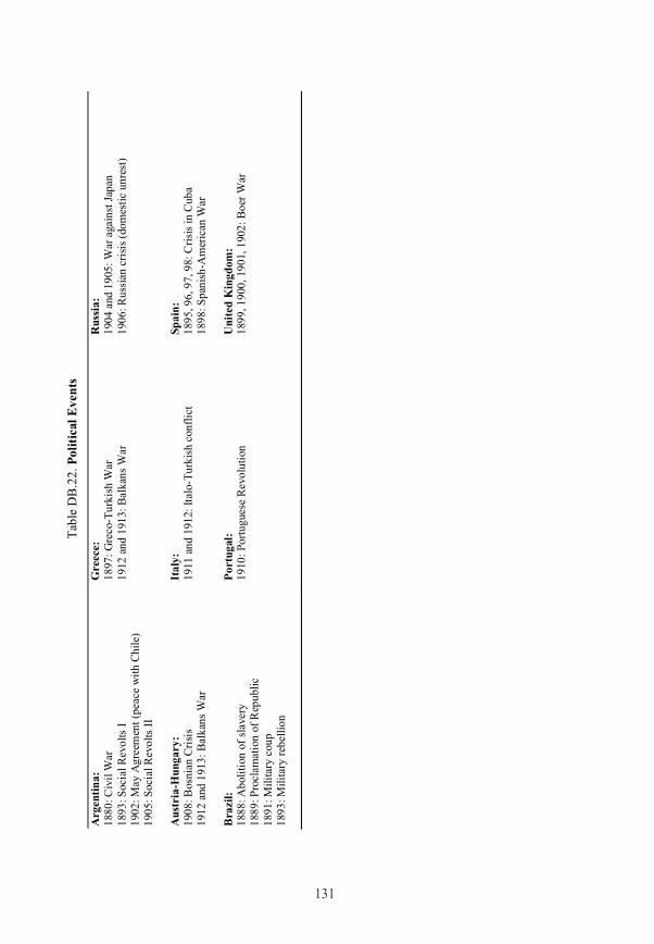
131

Tabl

e D

B.2

2. P

oliti

cal E

vent

s

Arg

entin

a:

1880

: Civ

il W

ar

1893

: Soc

ial R

evol

ts I

1902

: May

Agr

eem

ent (

peac

e w

ith C

hile

) 19

05: S

ocia

l Rev

olts

II

Gre

ece:

18

97: G

reco

-Tur

kish

War

19

12 a

nd 1

913:

Bal

kans

War

Rus

sia:

19

04 a

nd 1

905:

War

aga

inst

Jap

an

1906

: Rus

sian

cris

is (d

omes

tic u

nres

t)

Aus

tria

-Hun

gary

: 19

08: B

osni

an C

risis

19

12 a

nd 1

913:

Bal

kans

War

Ital

y:

1911

and

191

2: It

alo-

Turk

ish

conf

lict

Spai

n:

1895

, 96,

97,

98:

Cris

is in

Cub

a 18

98: S

pani

sh-A

mer

ican

War

Bra

zil:

1888

: Abo

litio

n of

sla

very

18

89: P

rocl

amat

ion

of R

epub

lic

1891

: Mili

tary

cou

p 18

93: M

ilita

ry re

belli

on

Port

ugal

: 19

10: P

ortu

gues

e R

evol

utio

nU

nite

d K

ingd

om:

1899

, 190

0, 1

901,

190

2: B

oer W

ar

132

Notes

1. In addition, the gold bonds were generally (if not systematically; see the case ofItaly) understood to be tax-free.

2. The data problem in Sussman and Yafeh (2000) discussed in the main text is anillustration of this sort of problem.

3. A companion problem is that the volatility of bonds with such options is affected bythe very existence of these options. This is an additional challenge for studies that,in the vein of Bordo and Rockoff (1996), have sought to rely on the CAPM and thuson the volatility of alternative securities. Obviously the approach here, which focusesonly on average yields, does circumvent this obstacle.

4. In 1901, Austria implemented a re-denomination of its currency from florin to crowns.Since this was a pure accounting change (the paper florin was worth 0.5 crown orKroner), one can report the series in either florins or crowns. The authors opted forthe florin.

5. For convenience, this study defines the “national unit” to be the milreis (rather thanthe contos or reis) and reports results in millions of milreis. The same procedure isused for Brazil. Of course, the Portuguese and Brazilian milreis did not necessarilycoincide, despite their common past.

6. See note 5 above.

7. Alfred Neymarck was in charge of collecting data on sovereign debts. In several ofthis Society’s meetings (it held congresses in all parts of the world including London,Paris and Chicago), Neymarck presented interesting papers on the topic. Yet whilehis contributions contain useful discussions of the methodological problems involved(see, for example, Neymarck, 1913) his figures were often reported with a five yearfrequency.

8. Apart from some well-maintained national series (such as those for France and theUnited Kingdom), all data required some cleaning up. One exception was the seriesfor Greece, for which our numbers, corrected with the help of Lyonnais figures,always came very close to numbers provided by Lazaretou (1993). To keep matterssimple, we thus follow those numbers whenever possible.

9. Among other things the Lyonnais tables used the Relazione des Direttore Generaledel Debito Pubblico alla Commissione di Vigilanza sul Rendicontodell’Administrazione del Debito Pubblico.

133

10. Calculations available upon request.

11. Komlos (1987) is the first source for modern estimates of national income in Austriaand Hungary. Good (1994) tries an indirect method to assess the wealth of alternativeparts of the monarchy. The other route is the hard one: two research projects conductedby Dr Schulze and Dr Kövler aim at estimating national accounts for both Austriaand Hungary before WWI. The data used for Austria come from Schulze (1997),while those for Hungary come from private communications.

12. Mitchell (1993) reports Dutch exports as larger than Dutch GDP.

13. Some series (the Scandinavian ones, for instance) are susceptible of furtherimprovement. The authors remain open to suggestions from other scholars workingin the field.

14. It is important to control for taxes: 13.2 per cent until the beginning of 1894 forboth bonds, 20 per cent until 1906 for the 5 per cent and until 1914 for the 3 percent, when the former 5 per cent was no longer taxable.

15. For a discussion of Austro-Hungarian spreads, see Flandreau (2004).

16. http://weber.ucsd.edu/~kgledits/Polity.html

134

135

Bibliography

ALONSO-BORREGO, C. and M. ARELLANO (1999), “Symmetrically Normalized InstrumentalVariable Estimation using Panel Data”, Journal of Business and Economic Statistics,17, pp. 36-49.

Annuaire Officiel des Agents de Change, various issues.

ARELLANO, M. and S. BOND (1991), “Some Tests of Specification for Panel Data: MonteCarlo Evidence and an Application to Employment Equations”, Review of EconomicStudies, 58, pp. 277-97.

ARELLANO, M. and O. BOVER (1995), “Another Look at the Instrumental Variable Estimationof Error-Components Models”, Journal of Econometrics, 68, pp. 29-51.

BAIROCH, P. (1993), Economics and World History: Myths and Paradoxes, HarvesterWheatsheaf, Hemel Hempstead, United Kingdom.

BAIROCH, P. (1976), Commerce extérieur et développement économique de l’Europe auXIXème siècle, Mouton and École des Hautes Études en Sciences Sociales, La Haye,Paris.

BAIROCH, P. (1974), “Geographical Structure and Trade Balance of European Foreign Tradefrom 1800 to 1974”, Journal of European Economic History, 3/3, pp. 597-68.

BALTAGI, B.H. (1986), “Pooling under Misspecification: Some Monte Carlo Evidence on theKmenta and the Error Components Techniques”, Econometric Theory, 2, pp. 429-440.

BARRO, R.J. (1987), “Government Spending, Interest Rates, Prices and Budget Deficits in theUnited Kingdom, 1701-1918”, Journal of Monetary Economics, 20, pp. 221-247.

BARRO, R.J. (1983), “Money and the Price Level under the Gold Standard”, Economic Journal,89, pp. 13-31.

BAXTER, R.D. (1871), National Debts, (2nd edition), Robert John Bush, London.

BAYOUMI, T. (1990), “Saving-Investment Correlations: Immobile Capital, Government Policy,or Endogenous Behavior”, IMF Staff Papers, 37 (2), June, pp. 360-387.

BLUNDELL, R. and S. BOND (1998), “Initial Conditions and Moment Restrictions in DynamicPanel Data Models”, Journal of Econometrics, 87, pp. 115-143.

BLUNDELL, R., S. BOND and F. WINDMEIJER (2000), “Estimation in Dynamic Panel Data Models:Improving on the Performance of the Standard GMM Estimators”, WP 00/12, TheInstitute for Fiscal Studies, London.

136

BORDO, M. and M. FLANDREAU (2003), “Core, Periphery, Exchange Rate Regimes andGlobalization”, in M. BORDO, A. TAYLOR and J. WILLIAMSON (eds.), Globalization inHistorical Perspective, Chicago University Press, Chicago, pp. 417-68.

BORDO, M. and H. ROCKOFF (1996), “The Gold Standard as a Good Housekeeper Seal ofApproval”, Journal of Economic History, Vol. 56, No. 2, June, pp. 389-428.

BOUVIER, J. (1961), Le Crédit Lyonnais de 1863 à 1882 : les années de formation d’unebanque de dépôts, Imprimerie Nationale, Paris.

BRAGA DE MACEDO, J., D. COHEN and H. REISEN (2002), Don’t Fix, Don’t Float, DevelopmentCentre Studies, OECD, Paris.

BRAGA DE MACEDO, J., A. FERREIRA DA SILVA and R. MARTINS DE SOUSA (2001), “War, Taxesand Gold: The Inheritance of the Real”, in M. BORDO and R. CORTES-CONDE,Transferring Wealth and Power from the Old to the New World, Cambridge UniversityPress, Cambridge, pp. 187-2.

Brazilian Yearbook (1908), First and second issues, Rio de Janeiro-London.

BREWER, J. (1990), The Sinews of Power. War, Money, and the English State 1688-1783,Harvard University Press, Cambridge, MA.

Bulletin de la Société Internationale de Statistique, various 19th century issues.

CAIRNCROSS, A. (1953), Home and Foreign Investment, 1870-1913: Studies in CapitalAccumulation, Cambridge University Press, Cambridge.

CALOMIRIS, C.W. (1988), “Price and Exchange Rate Determination During the GreenbackSuspension”, Oxford Economic Papers, 40:4, pp. 719-50.

CALVO, G. (2003), “Globalization Hazard and Delayed Reform in Emerging Markets”,Economia, 2.

CALVO, G. (1999), “Contagion in Emerging Markets: When Wall Street is a Carrier”, WorkingPaper, University of Maryland.

CAMERON, R.E. (1961), France and the Economic Development of Europe 1800-1914.Conquests of Peace and Seeds of War, Princeton University Press, Princeton, NJ.

CAMERON, R.E, V.I. BOVYKIN and B.V. ANAN’ICH (1992), International Banking 1870-1912,Oxford University Press, New York, NY.

CANOVAI, T. (1898), “Del Problema Finanziaro in Italia”, Nuova Antologia, 4th ser., 78, pp. 344-68.

CANTOR, R. and F. PACKER (1996), “Determinants and Impact of Sovereign Credit Ratings”,FRBNY Economic Policy Review, October, pp. 37-53.

CARRERAS, A. (1989), Estadisticas Historicas de Espana, Siglos XIX-XX, Fundacion BancoExterior, Madrid.

CLEMENS, M.A. and J. WILLIAMSON (2002), “Wealth Bias in the First Global Capital MarketBoom, 1870-1913”, NBER Working Paper.

CONANT, C. (1896), A History of the Banks of Issue, Putnam’s, New York, NY, and London.

CORPORATION OF FOREIGN BONDHOLDERS, Annual Report of the Council of the Corporationof Foreign Bondholders, London.

137

CORTES CONDE, R. (1989), Dinero, Deuda y crisis. Evolucion fiscal y monetaria en laArgentina, 1862-1890, Editorial Sudamericana, Buenos Aires.

COURTOIS, A. (1883), Manuel des fonds publics et des sociétés par actions, 8th edition,Garnier Frères, Paris.

CRÉDIT LYONNAIS (1998), “La Russie de 1881 vue par le Crédit Lyonnais”, Politique Etrangère,2/summer, pp. 411-22.

DAVIS, L. (1980), “The Investment Market 1870-1914. The Evolution of a National Market”,Journal of Economic History, 25:3, pp. 355-99.

DE CECCO, M. (1989), “The Italian Debt Conversion of 1906”, in R. DORNBUSCH and M. DRAGHI,Public Debt Management: Theory and History, Cambridge University Press,Cambridge, pp. 263-84.

DELLA PAOLERA, G. (1988), How the Argentine Economy Performed During the InternationalGold Standard: A Reexamination, Doctoral dissertation submitted to the Universityof Chicago.

DE MATTIA, R. (1978), Storia del capitale della banca d’Italia e degli Istituti Predecessori,Banca d’Italia, Rome.

DE MATTIA, R. (ed) (1967), I bilanci degli Instituti di Emissione Italiani dal 1845 al 1936,Banca d’Italia, Rome.

ECONOMIC AND FINANCIAL COMMITTEE (2003), “The Role of Financial Markets in PromotingSound Public Finances in EMU”, Ecofin Internal Report, Brussels.

The Economist, various issues.

L’Economiste Francais, various issues.

EDDIE, S. (1982), “Limits on the Fiscal Independence of Sovereign States in Customs Union:Tax Union Aspects of the Austro-Hungarian Monarchy, 1868-1911”, HungarianStudies Review, pp. 7-29.

EICHENGREEN, B. (1997), “Infrastructure Financing in Developing Countries: Lessons fromthe Railway Age”, in A. MODY (ed.), Infrastructure Delivery: Private Initiative andPublic Good, World Bank, Washington, DC.

EICHENGREEN, B. (1996), Globalizing Capital, A Short History of the International MonetarySystem, Princeton University Press, Princeton, NJ.

EICHENGREEN, B. (1992), “Trends and Cycles in Foreign Lending”, in H. SIEBERT (ed.), CapitalFlows in the World Economy, Möhr, Tübingen, pp. 3-28.

EICHENGREEN, B. and M. FLANDREAU (1997), The Gold Standard in Theory and History,2nd ed., Routledge, London.

EICHENGREEN, B. and M. FLANDREAU (1996), “The Geography of the Gold Standard” in J.BRAGA DE MACEDO, B. EICHENGREEN and J. REIS, Currency Convertibility: The GoldStandard and Beyond, Routledge Explorations in Economic History, Routledge,London and New York, NY, pp. 113-43.

138

EICHENGREEN, B., R. HAUSMAN and U. PANIZZA (2003), “Original Sin: the Pain, the Mysteryand the Road to Redemption”, forthcoming in B. EICHENGREEN and R. HAUSMAN, DebtDenomination and Financial Instability in Emerging Market Economies, Universityof Chicago Press, Chicago.

EICHENGREEN, B. and A. MODY (1998), “What Explains Changing Spreads on Emerging-Market Debt: Fundamentals or Market Sentiment?”, NBER Working Paper, No. 6408.

EICHENGREEN, B. and R. PORTES (2000), “Debt Restructuring With and Without the IMF” inA. MELTZER, Financial Institutions Advisory Commission Expert Papers, GovernmentPrinting Office, Washington, DC.

EICHENGREEN, B. and P. TEMIN (2000), “The Gold Standard and the Great Depression”,Contemporary History, 9, pp. 183-207.

ESTEVADEORDAL, A., B. FRANTZ and A.M. TAYLOR (2003), “The Rise and Fall of World Trade,1870-1939”, Quarterly Journal of Economics, Vol. 118, No. 2, May, pp. 359-407.

FELDSTEIN, M. and C. HORIOKA (1980), “Domestic Saving and International Capital Flows”,Economic Journal, 90:2, pp. 314-29.

Fenn’s Compendium of the English and Foreign Funds, Debts and Revenues of All Nations,Rewritten and brought to the latest date by R. L. NASH (1889), Effingham Wilson, London.

FERGUSON, N. (1998), The World’s Banker. The History of the House of Rothschild, Weidenfeldand Nicolson, London.

FERGUSON, N. and R. BATLEY (2001), “Political Risk and the International Bond Market betweenthe 1848 Revolution and the Outbreak of the First World War”, draft, Jesus College,University of Oxford, Oxford.

Financial Times, 3 January 2000, “Millennium Resolution: No More Funny Money”, byR. Dornbusch.

FISHLOW, A. (1985), “Lessons from the Past: Capital Markets During the 19th Century andthe Interwar Period”, International Organization, 39, 3, summer.

FLANDREAU, M. (2004), “The Logic of Compromise: A Non Optimum Currency AreaManifesto”, CEPR Discussion Paper.

FLANDREAU, M. (2003a), The Glitter of Gold. France, Bimetallism and the Emergence ofthe International Gold Standard 1848-1873, Oxford University Press, Oxford.

FLANDREAU, M. (ed.) (2003b), Money Doctors: The Experience of International FinancialAdvice 1850-2000, Routledge, London.

FLANDREAU, M. (2003c), “Crises and Punishment: Moral Hazard and the pre-1914 InternationalFinancial Architecture”, CEPR Discussion Paper No. 3742, in M. FLANDREAU (ed.),Money Doctors: The Experience of International Financial Advice 1850-2000,pp. 13-48, Routledge, London.

FLANDREAU, M. (2003d), “Caveat Emptor: Coping with Sovereign Risk without theMultilaterals”, CEPR Discussion Paper, in M. FLANDREAU, C.-L. HOLTFRERICH and H.JAMES (eds.), International Financial History in the Twentieth Century: System andAnarchy, pp. 13-48, Cambridge University Press, Cambridge.

139

FLANDREAU, M. (2000), “The Economics and Politics of Monetary Unions: A Reassessment ofthe Latin Monetary Union, 1865-71”, Financial History Review, Vol. 7, No. 1, pp. 25-43.

FLANDREAU, M. (1996), “The French Crime of 1873: An Essay on the Emergence of theInternational Gold Standard”, Journal of Economic History, Vol. 56, No. 4, pp. 862-897.

FLANDREAU, M., J. LE CACHEUX and F. ZUMER (1998), “Stability Without a Pact? Lessons fromthe European Gold Standard 1880-1913”, Economic Policy, Vol. 13, issue 26, pp. 117-162.

FLANDREAU, M. and C. RIVIÈRE (1999), “La grande retransformation? Contrôles de capitauxet intégration financière internationale 1880-2000”, in M. FLANDREAU (ed.) Un siècled’architectures financières internationales, a special number of the review Economieinternationale, No. 78.

FLANDREAU, M. and N. SUSSMAN (2003), “Old Sins: Exchange Rate Clauses and EuropeanForeign Lending in the 19th Century”, forthcoming in B. EICHENGREEN and R. HAUSMAN(eds.), The Problem of Original Sin, University of Chicago Press, Chicago.

FORD, A.G. (1962), The Gold Standard 1880-1914, Britain and Argentina, Clarendon, Oxford.

FOREMAN-PECK, J. (1983), A History of the World Economy: International EconomicRelations Since 1850, Barnes & Noble, Totowa, NJ.

FREEMAN J., J. HAYS and H. STIX (1999), “Democracy and Markets: The Case of ExchangeRates”, Working Papers 39, Oesterreichische Nationalbank (Austrian National Bank).

GALLAROTTI, G. (1995), The Anatomy of an International Monetary Regime, Oxford UniversityPress, Oxford.

GERLOFF, W. (1911), Die Finanz und Zollpolitik des Deutschen Reiches, Verlag von GustavFischer, Jena.

GERSCHENKRON, A. (1962), Economic Backwardness in Historical Perspective, BelknapPress, Cambridge, MA.

GILLE, B. (1967), Histoire de la Maison Rothschild. 1848-1870, Droz, Geneva.

GOLDSMITH, P.H. (1924), Argentina, an Authorized Digest of “El desarrollo economico dela Republica Argentina en los ultimos cincuenta Anios”, Inter-America Press, NewYork, NY.

GOOD, D. (1994), “The Economic Lag for the Habsburg Successor States, 1870-1910”, Journalof Economic History, Vol. 54, No. 4, December, pp. 869-891.

GREGORY, P. (1994), Before Command: An Economic History of Russia before Emancipationto the First Five Years of the Five Years’ Plan, Princeton University Press, Princeton, NJ.

GREGORY, P. (1982), Russian National Income 1885-1913, Cambridge University Press,New York, NY.

HAUPT, O. (1894), Arbitrages et parités, traité des opérations de banque, 8th ed., Truchy,Paris.

HERBAULT, N. (1901), “Le contrôle international en Egypte, en Turquie et en Grèce”, CongrèsInternational des Valeurs Mobilières, No. 166.

HOFFMANN, W. (ed.) (1965), Das Wachstum der deutschen Wirtschaft seit der Mitte des 19.Jahrunderts, Springer, Heidelberg.

140

HOMER, S. and R. SYLLA (1991), A History of Interest Rates, Rutgers University Press, Rutgers.

INSTITUT NATIONAL DE LA STATISTIQUE ET DES ÉTUDES ÉCONOMIQUES (INSEE) (1966), AnnuaireStatistique de la France, Résumé rétrospectif, INSEE, Paris.

INSTITUTO BRASILEIRO DE GEOGRAFIA E ESTATÍSTICA (IBGE) (1986), Series EstatísticasRetrospectivas, IBGE, Rio de Janeiro.

Investor’s Monthly Manual, a companion supplement to The Economist, various issues.

IRWIN, D. (1996), Against the Tide: An Intellectual History of Free Trade, Princeton UniversityPress, Princeton, NJ.

JENKS, L.H. (1927), The Migration of British Capital to 1875, Knopf, New York, NY.

JOHANSSON, O. (1967), The Gross Domestic Product of Sweden and its Composition, 1861-1955, Almqvist & Wiksell, Stockholm.

Journal of Economic History (2000), Special Issue on institutions.

KAMIN, S.B. and K. VON KLEIST (1999), “The Evolution and Determinants of Emerging MarketCredit Spreads in the 1990s”, Boards of Governors of the Federal Reserve System,International Finance Discussion Papers, No. 653.

KELLY, T. (1998), “Ability and Willingness to Pay in the Age of Pax Britannica, 1890-1914”,Explorations in Economic History, 35:1, pp. 31-58.

KINDLEBERGER, C.P. (1988), Keynesianism vs. Monetarism and other Essays in FinancialHistory, Allen & Unwin, London, Boston and Sydney.

KLOVLAND, J.T. (1994), “Pitfalls in the Estimation of the Yield on British Consols, 1850-1914”, Journal of Economic History, Vol. 54, No. 1, March, pp. 164-87.

KMENTA, J. (1986), Elements of Econometrics, Macmillan, New York, NY.

KOEHLER, B. (1999), Ludwig Bamberger: Revolutionär und Bankier, Deutsche Verlags-Anstalt, Stuttgart.

KOKOVTSOV, V.N. (1933), Iz moego proshalgo, 2 Vol., Kokovtsov, Paris.

KOMLOS, J. (1987), “Financial Innovation and the Demand for Money in Austria-Hungary,1867-1913”, Journal of European Economic History, Vol. 16, No. 3, winter, pp. 587-605.

KOSTELENOS, G.C. (1995), Money and Output in Modern Greece, 1858-1938, Centre ofPlanning and Economic Research, Athens.

KRASNER, S. (1983), International Regimes, Cornell University Press, Ithaca.

KRÄUSSL, R. (1999), “Sovereign Ratings and Their Impact on Recent Financial Crises”,mimeo, Centre for Financial Studies, Frankfurt am Main.

LAFFITTE, J. (1824), Réflexions sur la réduction de la rente et sur l’état du crédit, BossangePère, Paris.

LAINS, P. and J. REIS (1991), “Portuguese Economic Growth, 1833-1985: Some Doubts”,Journal of European Economic History, 20:2, pp. 441-453.

LAZARETOU, S. (1993), “Monetary and Fiscal Policies in Greece: 1833-1914”, Journal ofEuropean Economic History, 22:2, pp. 285-311.

141

Le Rentier, various issues.

LEROY-BEAULIEU, P. (1899), Traité de la Science des Finances, 6th edition 2 Vol., Guillaumin,Paris.

LEROY-BEAULIEU, P. (1878), Traité de la Science des Finances, 2nd edition, 2 Vol., Guillaumin,Paris.

LÉVY, R.G. (1911), Banques d’émission et Trésors publics, Économiste Européen, Hachette,Paris.

LÉVY-LEBOYER, M. and F. BOURGUIGNON (1985), L’Economie française au XIXe siècle,Economica, Paris.

LIESNER, T. (1989), One Hundred Years of Economic Statistics, The Economist Publications,Facts on File, London.

LOPEZ-CORDOVA, J. and C. MEISSNER (2000), “Exchange-Rate Regimes and International Trade:Evidence from the Classical Gold Standard”, draft, University of California at Berkeley.

MCCLOSKEY, D. (1970), “Did Victorian Britain Fail?”, Economic History Review, Vol. 23,No. 3, December, pp. 446-459.

MCKINNON, R. (1996), The Rules of the Game. International Money and Exchange Rates,MIT Press, Cambridge, MA.

MADDEN, J. (1985), British Investment in the United States 1860-1880, Garland Publishing,New York, NY.

MADDISON, A. (2001), The World Economy, A Millennial Perspective, Development CentreStudies, OECD, Paris.

MADDISON, A. (1991), Dynamic Forces in Capitalist Development, A Long-Run ComparativeView, Oxford University Press, Oxford.

MARTIN ACEÑA, P. (2000), “The Spanish Monetary Experience, 1848-1914” in P. MARTINACEÑA and J. REIS (eds.) Monetary Standards in the Periphery: Paper, Silver andGold, 1854-1933, St. Martin’s Press, New York, NY, pp. 112-51.

MATA, E. (1993), As Finanças Publicas Portuguesas da Regeneraçao à Primeira GuerraMundial, Presençà, Lisboa.

MATSUKATA, M. (1899), Report on the Adoption of the Gold Standard in Japan, GovernmentPress, Tokyo.

MÁTYÁS, L. and P. SEVESTRE (eds.) (1996), The Econometrics of Panel Data, A Handbook ofthe Theory with Applications, Second Revised Edition, Kluwer Academic Publishers,Netherlands.

MAURO, P., N. SUSSMAN and Y. YAFEH (2002), “Emerging Markets Spreads: Then vs. Now”,Quarterly Journal of Economics, 117 (2), pp. 695-733.

MITCHELL, B.R. (1993), International Historical Statistics: Europe 1750-1988, StocktonPress, New York, and International Historical Statistics: The Americas, 1750-1988,Macmillan, New York, NY.

MITCHELL, B.R. (1990), British Historical Statistics, Cambridge University Press, Cambridge.

142

MOODY’S INVESTORS SERVICE (2002), Moody’s Statistical Handbook: Country Credit, Moody’s,New York, NY.

MULHALL, M.G. (1896) Industries and Wealth of Nations, Longmans, Green and co., London,New York, NY.

MULHALL, M.G. (1892), The Dictionary of Statistics, Thoemmes Press, London.

MULHALL, M.G. (1887), Handbook of the River Plate, Comprising the Argentine Republic,Uruguay and Paraguay, E.T. Mulhall, Buenos Aires.

NEAL, L. (1990), The Rise of Financial Capitalism: International Capital Markets in theAge of Reason, Cambridge University Press, Cambridge.

NEYMARCK, A. (1913), “La statistique internationale des valeurs mobilières”, (IXème Rapportde M. Alfred Neymarck), Bulletin de l’Institut international de statistique, Vol. XIX,pp. 201-475, Van Stockum, The Hague.

NEYMARCK, A. (1887), Les dettes publiques européennes, Guillaumin, Paris.

NOGARO, B. (1940), “L’étalon or n’a jamais existé”, Revue d’Economie Politique, 2, pp. 164-84, spring.

NORTH, D. and B. WEINGAST (1989), “Constitutions and Commitment: Evolution of InstitutionsGoverning Public Choice in Seventeenth Century England”, Journal of EconomicHistory, XLIX (4), December.

NUNES, A., E. MATA and N. VALERIO (1989), “Portuguese Economic Growth”, The Journal ofEuropean Economic History, Vol. 18, No. 2, autumn, pp. 291-330.

O’BRIEN, P.K. (2001), “Fiscal Exceptionalism: Great Britain and its European Rivals fromCivil War to Triumph at Trafalgar and Waterloo”, London School of Economics,Working Paper No. 65/01.

OBSTFELD, M. and A. TAYLOR (2003a), “Sovereign Risk, Credibility and the Gold Standard:1870-1913 versus 1925-1931”, NBER Working Paper, forthcoming in the Economic Journal.

OBSTFELD, M. and A. TAYLOR (2003b), “Globalization and Capital Markets”, NBER WorkingPaper, in M. BORDO, A. TAYLOR and J. WILLIAMSON, Globalization in HistoricalPerspective, pp. 121-187, University of Chicago Press, Chicago.

OBSTFELD, M. and A. TAYLOR (1998), “The Great Depression as a Watershed: InternationalCapital Mobility over the Long Run”, CEPR Discussion Paper.

OECD (2002), Japan (OECD Economic Studies), OECD, Paris.

OMAN, C., C. FOY and J. BRAGA DE MACEDO (eds.) (2003), Development is Back, OECDDevelopment Centre Studies, OECD, Paris.

O’ROURKE, K. and J. WILLIAMSON (1999), Globalization and History: the Evolution of a19th Century Atlantic Economy, MIT Press, Cambridge, MA.

PELAEZ, C.M. and W. SUZIGAN (1976), Historia monetaria do Brasil. Analise da politica,comportamento e instituiçoes monetarias, IPEA., Rio de Janeiro.

PRADOS DE LA ESCOSURA, L. (1995), “Spain’s Gross Domestic Product: 1850-1993: QuantitativeConjectures and Appendix”, Working Paper, 95-05 and 95-06, Universidad Carlos III,Madrid.

143

RAFFALOVICH, A. (1904), “The Financial Situation in Russia”, Economic Journal, Vol. 14,No. 56, December, pp. 625-632.

REINHART, C. (2002), “Default, Currency Crises and Sovereign Credit Ratings”, NBER WorkingPaper, No. 8738.

REIS, J. (1996), “First to Join the Gold Standard, 1854” in J. BRAGA DE MACEDO, B. EICHENGREENand J. REIS (eds.), Currency Convertibility: The Gold Standard and Beyond, RoutledgeExplorations in Economic History, Vol. 3, pp. 164-84, Routledge, London and NewYork, NY.

REISEN, H. and J. VON MALTZAN (1999), Boom and Bust and Sovereign Ratings, OECDDevelopment Centre, Technical Paper No. 148, Paris.

RITZMANN-BLICKENSTORFER, H. (1996), Historical Statistics of Switzerland, Chronos, Zürich.

RODRIK, D. (1998), “Why do More Open Economies Have Bigger Governments”, Journal ofPolitical Economy, Vol. 106, No. 5, October, pp. 997-1032.

ROSOVSKY, H. (1961), Capital Formation in Japan, 1868-1940, Free Press of Glencoe, NewYork, NY.

ROULLEAU, G. (1914), Les Règlements par effets de commerce en France et à l’étranger,Dubreuil, Paris.

SCHNEIDER, J., O. SCHWARZER and M. DENZEL (1997), Währungen der Welt VII, Franz SteinerVerlag, Stuttgart.

SCHNEIDER, J., O. SCHWARZER and F. ZELLFELDER (1991), Währungen der Welt I, 3 Vol., FranzSteiner Verlag, Stuttgart.

SCHULZE, M.S. (1997), “Reestimating Austro-Hungarian GDP: Methods and Sources”,Working Paper, London School of Economics.

SCHUMPETER, J.A. (1939), Business Cycles. A Theoretical, Historical and Statistical Analysisof the Capitalist Process, 2 Vol., McGraw-Hill Book Company, New York, NY, and London.

SCHWARTZ, A., (2003), “Comment on Bordo and Flandreau” in M. BORDO, A. TAYLOR and J.WILLIAMSON, Globalization in Historical Perspective, NBER, University of ChicagoPress, Chicago.

SMITS, J.P., E. HORLINGS and J.L.VAN ZANDEN (1997), “The Measurement of Gross NationalProduct and its Components, The Netherlands, 1800-1913”, Research Memorandum,N.W. Posthumus Insituut, Netherlands Graduate School for Economic and SocialHistory.

SOETBEER (1889), Matériaux pour faciliter l’intelligence et l’examen des rapportséconomiques des métaux précieux et de la question monétaire, Berger Levrault,Paris and Nancy.

SPINELLI, F. and M. FRATIANNI (1991), Storia monetaria d’Italia. L’evoluzione del Sistemamonetario e bancario, Mondadori, Milan.

Statesman’s Year Book, annual from 1866, MacMillan, London.

STIGLITZ, J.E. and A. WEISS (1981), “Credit Rationing in Markets with Imperfect Information”,American Economic Review, Vol. 71, No. 3, June, pp. 393-410.

144

SUSSMAN, N. and Y. YAFEH (2000), “Institutions, Reforms and Country Risk: Lessons fromJapanese Government Debt in the Meiji Period”, Journal of Economic History, 60, 2,pp. 442-467.

SUSSMAN, N. and Y. YAFEH (1999), “Institutions économiques et intégration des marchésinternationaux de capitaux : Le cas du Japon pendant l’ère Meiji” in M. FLANDREAU(ed.) Un siècle d’architectures financières internationales, a special number of thereview Economie internationale, 0:78, pp. 85-103.

SUZUKI, T. (1994), Japanese Government Loan Issues on the London Capital Market 1870-1913, Athlone Press, London.

SVERIGES RIKSBANK (1931), Sveriges Riksbank, 1668-1918. Bankens tillkomst ochverksamhet, Stockholm, P.A. Norstedt.

TANZI, V. (ed.) (1990), Fiscal Policy in Open Developing Economies, International MonetaryFund, Washington, DC.

TANZI, V. (1989), “Lags in Tax Collection and the Case for Inflationary Finance: Theory withSimulations” in M.I. BLEJER and K.-Y. CHU (eds.), Fiscal Policy, Stabilization, andGrowth in Developing Countries, International Monetary Fund, Washington, DC.,pp. 208-37.

TATTARA, G. (2003), “Paper Money but a Gold Debt: Italy on the Gold Standard”, Explorationsin Economic History, 40:2, pp. 122-42.

TATTARA, G. (1999), “Was Italy Ever on Gold?”, in P.M. ACENA and J. REIS (eds.), MonetaryStandards in the Periphery, Paper, Silver and Gold 1854-1933, Macmillan, London,pp. 18-68.

THÉRY, E. (1887), Les dettes publiques en Europe, Guillaumin, Paris.

TOMII, M. (1898), “Etat de la codification au Japon”, Bulletin de la Société de LégislationComparée, 3, pp. 3-11.

TOMZ, M. (2001), “How Do Reputations Form: New and Seasoned Borrowers in InternationalCapital Markets”, draft, Stanford University.

TRIFFIN, R. (1964), “The Myth and Realities of the So-called Gold Standard”, in R. TRIFFIN,The Evolution of the International Monetary System: Historical Reappraisal andFuture Perspectives, Princeton University Press, Princeton, NJ.

TRINER, G. (2001), “International Capital and the Brazilian Encilhamento, 1889-1893:An Early Example of Contagion among Emerging Capital Markets”, mimeo, RutgersUniversity.

VILLANOVA VILLELA, A. and W. SUZIGAN (1973), Política do governo e crescimento daeconomia brasileira: 1889-1945, IPEA, INPES, Rio de Janeiro.

WAGNER, A. (1863), Die Ordnung des österreichischen Staatshaushaltes mit besondererRücksicht auf den Ausgaben-Etat und die Staatsschuld, Gerold, 1863 and Brandstätter,1984, Vienna.

WEBER, M. (1904), Die Protestantische Ethik und der “Geist” des Kapitalismus, SiebesternTaschenbuch, Hamburg.

ZAMAGNI, V. (1997), “Ricostruzione della serie del debito pubblico italiano, 1861-1946”, mimeo.

OECD PUBLICATIONS, 2, rue André-Pascal, 75775 PARIS CEDEX 16PRINTED IN FRANCE

(41 2004 03 1 P) ISBN 92-64-01534-5 – No. 53489 2004

Th

e M

ak

ing

of G

lob

al F

ina

nc

e 1

880-1

913

OECD's books, periodicals and statistical databases are now available via www.SourceOECD.org, our online library. This book is available to subscribers to the following SourceOECD themes:DevelopmentFinance and Investment/Insurance and PensionsGeneral Economics and Future StudiesAsk your librarian for more details of how to access OECD books on line, or write to us atSourceOECD@oecd.org

This book traces the roots of global financial integration in the first “modern” eraof globalisation from 1880 to 1913. It analyses the direction, destinations andorigins, of international financial flows in order to determine the domestic policychoices that either attracted or deterred such flows to developing countries.

The book deposes the idea that the gold standard and other institutionalarrangements were the key to attracting foreign investment, pointing to thestability and probity of political systems as much more important. One of the majorconclusions is that the successful management of international financialintegration depends primarily on broad institutional and political factors, as well ason financial policies, rather than simply opening or closing individual economies tothe international winds.

The Making of Global Finance 1880-1913 can serve as a valuable tool to current-day policy dilemmas by using historical data to see which policies in the past ledto enhanced international financing for development. It also includes historicaldata that will interest all scholars of economics and economic history, as well asthe casual reader.

Development Centre Studies

The Making of Global Finance 1880-1913

ISBN 92-64-01534-541 2004 03 1 P-:HSTCQE=UVZXYU:

www.oecd.org

«Development Centre Studies

The Making of Global Finance1880-1913

By Marc Flandreau and Frédéric Zumer

This work is published under the auspices of the OECDDevelopment Centre. The Centre promotes comparative development analysis and policy dialogue, as described at:

www.oecd.org/dev