The magnitude of errors at flow measurement stations

Reginald W. Herschy Senior Engineer, Water Resources Board, Reading, United Kingdom

Abstract. An assessment of the accuracy of hydrometric data produced from flow measurement stations is important to the users of the data. This is particularly so in the case of water resources development.

The paper uses a statistical approach and outlines simple statistical methods for obtaining the error in a single determination of discharge at both velocity-area stations and at weirs and flumes. In connexion with velocity-area stations, a method of obtaining the standard error of the stage-discharge curve is discussed and a statistical test for significance of check gaugings is demonstrated. Statistical definitions as they apply to hydrometry are included in an appendix.

GRANDEUR DES ERREURS DANS LES STATIONS DE JAUGEAGE DES DEBITS

Résumé. Il importe que les utilisateurs des données hydrométriques fournies par les stations hydrométriques (de jaugeage) puissent évaluer la précision de ces données. Cela est particulière- ment vrai lorsqu’il s’agit de mise en valeur des ressources hydrauliques.

Dans cette communication, l’auteur aborde le problème sous un angle statistique et expose des méthodes statistiques simples qui permettent de déterminer l’erreur lors d’une seule mesure du débit, tant aux stations utilisant les moulinets qu’aux déversoirs et autres jaugeurs. A propos des stations utilisant les moulinets, l’auteur étudie une méthode permettant d’obtenir l’erreur type de la courbe de tarage et indique un test statistique grâce auquel il est possible de déterminer la signification des jaugeages de vérification. Des définitions statistiques s’appliquant I’hydro- métrie sont groupées dans une annexe.

MAGNITUD DE LOS ERRORES EN LAS ESTACIONES DE MEDICI~N DE CAUDAL

Resumen. Es importante para los que utilizan los datos hidrométricos obtenidos en las estaciones de medición de caudal el conocer la precisión de dichos datos. Esto sucede especialmente en el caso del estudio de los recursos de agua.

Esta comunicación utiliza un enfoque estadístico y destaca los métodos estadísticos simples para averiguar el error en una Única determinación de caudal, tanto en las estaciones de velocidad-área, como en los vertederos y otros dispositivos de medida. Respecto a las estaciones de velocidad-&ea, se discute un método para obtener el error normal en la curva de nivel-caudal y se muestra un ensayo estadístico para determinar la significación de las calibraciones de verifica- ción. En el apéndice se han incluido las definiciones estadísticas utilizadas,

BEAMYHHbI OLUHEOK H A CTAHqHBX, H3MEPHlDIIJMX PACXOAbI

1 o9

R. W. Herschy

INTRODUCTION

By accuracy of flow measurement is meant the degree of agreement between the apparent flow as measured and the actual flow. The estimation of the accuracy of a measurement, therefore, consists in determining the likely magnitude of the differ- ence between the apparent and the actual flow. It is not confined to a single measurement of the instantaneous flow but also to daily mean discharge,monthly mean discharge and average flow. The International Organization for Standardization (ISO) [refs. 1,2] states.

“No measurement of a physical quantity can be free from uncertainties which may be associated with either systematic bias caused by errors in the standardizing equipment or a random scatter caused by a lack of sensitivity of the measuring equipment. The former is unaffected by repeated measurements and can only be reduced if more accurate equipment is used for the measurements. Repetition does, however, reduce the error caused by random scatter. The precision of the average ‘n’ repeated measurements is 6 times better than that of any of the points by themselves. “When considering the possible uncertainty of any measurement of the discharge

in an open channel, it is not possible to predict this uncertainty exactly but an analysis of the individual measurements which are required to obtain the discharge can be made and a statistical estimate made of the likely tolerance. A 95 per cent tolerance on measurement may be defined statistically as the bandwidth around the calculated value which, on an average of nineteen times out of twenty, can be expected to include the true value .”

For computation of errors, therefore, the over-all tolerance should be based on the 95 per cent confidence level and this may be taken as approximately twice the standard deviation. However, care is required to ensure that individual or partial errors are used at the same confidence level. For current meter stations it is suggested that all errors are considered initially at 68 per cent confidence level and only at the final stages doubled to give the 95 per cent confidence level. In the case of weirs and flumes, however, where the coefficient of discharge is determined in the laboratory and random or systematic errors can be carefully controlled in the field, it is convenient to use partial errors at the 95 per cent confidence level.

KINDS OF ERRORS

Errors may be either random or systematic. The former are produced by purely chance fluctuations in conditions and the latter are associated with a particular instrument or method of measurement. In the discussion of errors in stream gauging it is assumed that the random errors involved are distributed according to the normal or Gaussian distribution. Fortunately any departure from this law has to be very severe before statistical tests based on it become invalid. In stream gauging certain systematic errors behave like random errors and may be assessed in a similar way. For

110

The magnitude of errors at flow measurement stations

instance, in a measuring structure, small systematic errors may occur in the coeffi- cient of discharge which may be attributable to variations in the surface finish of the structure or to the approach conditions, etc.

OVER-ALL TOLERANCE ON DISCHARGE

Estimating the tolerance on a single determination of discharge depends on estima- tion of the partial errors pertaining to various parts of the measurement. Some of these may be of widely varying ascertained errors and others may be the operator’s own estímate of the accuracy of his work. Attention should be given, therefore, to evaluating partial errors as accurately as possible on site.

CONTRIBUTING (PARTIAL) ERRORS

For a single measurement of discharge by current meter the contributing errors are as

Errors (standard deviations expressed as percentages) Errors in determination of velocity

follow [l] :

X, = Error due to the choice of the number of verticals Xf = Error due to the choice of duration of exposure of current meter X, = Error due to the choice of the number of points in a vertical.

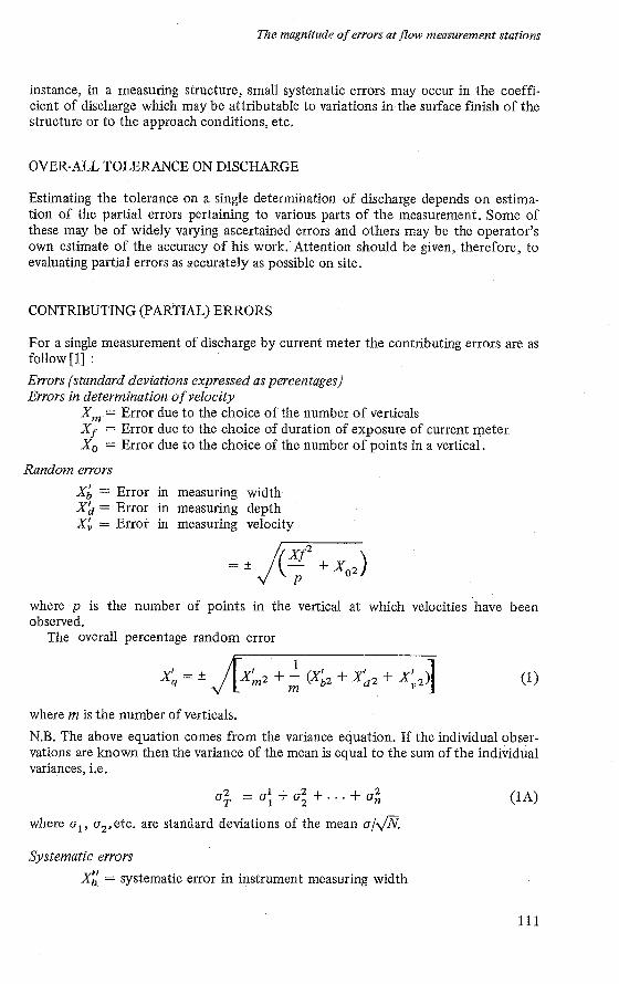
Random errors XL = Error in measuring width Xh = Error in measuring depth X: = Error in measuring velocity

where p is the number of points in the vertical at which velocities ’have been observed.

The overall percentage random error

where m is the number of verticals. N.B. The above equation comes from the variance equation. If the individual obser- vations are known then the variance of the mean is equal to the sum of the individual variances, i.e.

where o1, o,,etc. are standard deviations of the mean a/@.

Systematic errors = systematic error in instrument measuring width

111

R. W. Herschy

= systematic error in instrument measuring depth A$‘ = systematic error in current meter.

The overall percentage systematic error

x” 4 = * &xiz + xi2 + X’:2). The overall error is then

X Q = d m . (3)

Random errors Suggested values [l, 31 for the above errors are as follows. These values were suggested by the British Standard Committee after considering all the available data.

X, Error due to the number of verticals

m

8 f 5 per cent 15 f 3 per cent 50 k 1 per cent

Xf Error due to choice of duration of exposure of current meter

For an exposure time of 40 seconds or 100 counts approximately the recommenda- tion is Xi = -+ 6 per cent.

Xo Error due to the choice of the number of points in a vertical

Method XO velocity distribution 0.5 per cent 2 point 3.0 per cent 1 point (0.6 depth) 3.5 per cent

XL Error in measuring width Errors in measuring width, either between verticals or in total width, by line or winch are usually small and normally negligible and a value off 0.50 per cent is suggested.

Xi Error in measuring depth These are best determined on site but normally a tolerance of k 1 per cent should be possible to attain at large values of depth and f 3 per cent at shallow depths although repeated measurements may be necessary to reduce the tolerance, noting that the error for n repeated measurements is +times better than that for a single measurement. For example a measurement repeated 4 times halves the error of that of a single measurement.

Systematic errors The possibility of systematic errors occurring in thelinstruments measuring velocity, depth,width, level, zero etc. should be carefully examined from time to time and

112

The magnitude of errors at flow measurement stations

such errors corrected where necessary. The errors in Xz and Xz should-be limited to C 1/2 per cent but these errors are usually so small that they may be neglected. Again a field test is recommended to evaluate these errors.

X; The error in the current meter This error may be defined as the difference between the meter’s tank rating and its performance in the field. There may also be a small systematic error in the tank calibration which is usually negligible. The rating of a current meter may takeeither the usual form of individual rating or the more recently proposed group rating. Lambie [4] and Smoot and Carter (51 suggested that a group rating is as accurate as an individual rating and that errors are primarily due to errors in the rating procedure. Part of the error may therefore be random and part systematic. Either way, however, makes little or no difference to the actual computation of the over-all error in discharge. The tests carried out by Lambie [4] involved some 130 ratings totalling some

3,200 data points for 15 used Watts cup-type meters. Smoot and Carter [5] carried out tests with 140 new Price meters giving about 2,200 data points and Grindley in tests at the Hydraulics Research Station, England, used 18 new Watts cup-type meters and 120 new propeller meters from three different manufactures. From all of these tests the following table of percentage errors is suggested for both new cup-type meters and new propeller meters (standard errors at 68 per cent confidence level),for both individual and group ratings.

Percentage standard error at 68 per cent confidence level

(coefficient of variation) Velocity

m/sec ft/sec Individual rating Group rating

0.08 0.25 3 4 0.1 5 0.50 1 2 0.25 0.75 1 1 0.30 1 .o0 1 1 above above 0.30 1 .o0 O .5 1

Example: It is required to calculate the over-all tolerance XQ on an individual discharge measurement from the following particulars.

Number of verticals used 15 No. exposure of meter 40 sec (2 exposures made) method of measurement 2 point average velocity above 1 ft sec (0.30 m) individual rating

From the above information the partial errors (at 68 per cent confidence level) can be assessed.

113

R. W. Herschy

Random:

Y m = f 3 %

6% Y* =- ~ (2 exposures)

= ? 4.25 % x; = 2 3 % Tb = f 0.5 % & = k 2.5 % Tv = kj(? 4.252 + 3')

Systematic:

X" = _+ 0.5 % X: = f 0.5 %

b

X: = k 0.5 %(from table above).

The overall random error in discharge is then

1 m

x' = f J(xh2 + - (Xi' + XL' + Xi2)) 4

= +J[32 + 1/15 (0.5' + 2.5' + 18)]

= +_ 3.25 %. The overall systematic error in discharge is

x" 4 = _+ J(X12 + x;' + XY2) = f J(0.52 + 0.5' + OS2) = k 1 %approx.

The overall standard error is then

XQ = f J(Xi2 + X:2) = fJ(3,252 + 12) = k 3.5 %approx.

XQ at 95 % confidence level = 2 X 3.5 = k 7 % .

114

The magnitude of errors at flow measurement stations

I

5 c Rating Equation: Q + 125.6(h - 0.2)’’9’ I

I I I I I I I I I I I I 1 I l l l l 30 40 50 1 O 0 200 300 400 500 600

Q (CUSECS)

NOTE:

95 per cent confidence limits for Se - 2 Se 2 S e x Q

= 100 e.g. at.Q = 500 cusecs

2 Se - 2 x 6.4 x 500 64 =UseCS 100

Similarly for 2 Smr - 2 x 1.85 x NO 1 O0 - 18.5 cusecs

Figure 1. Stage-discharge relation

115

R. W. Herschy

h

.6 v

.E c ßJ 13 U

.3 C .- L

2 !z -13.* .7 4

5 .c u

o .-

2Smr- rp

.2

L

-400 .

-300

1: .ll -200

- If

-100

- - -50

-40

-30 2Smr

- -10 -!i

1500

=2X1.85 - 3.7% 1 O

.14 .10 .9 .18

.8 16.

.5

2Se I 12.8% -

5 10

.17

15

P E RCENTAGE DEVI AT ION NOTE 2 Se represents the probable magnitude of error (at 95 per cent confidence level i.e. 19 times out of 20) in the individual gaugings made in determination of the rating equation.

2 Smr represents the probable magnitude of error (at 95 per cent confidence level i.e. 19 times out of 20) in the discharges taken from the rating equation.

Figure 2. Deviation diagram

116

The magnitude of errors at flow measurement stations

That is on 68 times out of 100 (1 standard deviation) a single measurement of discharge made under these tolerances should be within 5 3.5 per cent of the true discharge; 95 times out of 100 (2 standard deviations) it should be within & 7 per cent of the true discharge and 99.7 times out of 100 it should be within f 10.5 per cent of the true discharge (3 standard deviations). An approximate relationship between the over-all standard error and the number

of verticals in the cross-section, after Carter [3] is shown graphically in Fig. 3 for the 0.6 method and the 0.2 and 0.8 method and one exposure of 40 seconds. The error in the single current meter is taken from the tableAthou@ the over-all standard error can be reduced by repeating observations, as stated earlier, the curves in Fig. 3 show clearly that the error is also reduced by increasing the number of verticals. For the above example the 0.2-0.8 curve gives a standard error for 15 verticals of: 7.5 per cent at the 95 per cent confidence level.

STAGE-DISCHARGE CURVE The stage-discharge curve being a curve of best fit should, unless some of the individual gaugings actually lie on the curve, be more accurate than any of the individual gaugings. One method of assessing this accuracy statistically is suggested as follows : Fig. 1 shows a stages-discharge curve plotted on logarithmic graph paper from

the gaugings numbers 1 to 12 in Table A (Appendix) [6]. Check gaugings 13 to 18 are also shown in Fig. 1 and indicated by circles. The equation of the curve is computed in the usual manner by the root mean square method [l] and is Q = 125.6(h-0.2). The standard error of estímate (Se) expressed as a percentage (also referred to as the coefficient of variation) is calculated as shown in Tables A and B, to be 6.4 per cent at 68 per cent confidence level and the standard error of the mean relationship (Smr) is calculated to be 1.85 per cent at the same confidence level. This is more clearly presented in Fig. 2 where the central ordinate represents the stage discharge relation and the abscissa represents percentage deviations of the observed discharges from the central ordinate. The outer limits in Figs. 1 and 2 represent the tolerance on a single gauging at the 95 per cent confidence level and should include 19 out of 20 of the observations made in the determination of the stage discharge relation. Also, pro- vided that there is no change in the hydraulic characteristics of the station, such as change in the control section, then 19 out of 20 of all check gaugings should fall between these limits. The inner limits on Figs. 1 and 2 represent the tolerance at 95 per cent confidence level on discharges taken from the stage discharge relation. That is in 19 cases out of 20 the true value of Q in the population lies between the limits of & 2Smr. Usually 2Se or 2Smr may be conveniently computed for more than one range but normally more gaugings are taken at the lower end of a stage discharge curve and since 2Smr gets smaller as the number of gaugings increases its value may be more or less uniform for the entire range of stage.

The above computation may of course be conveniently performed by computer and Table D shows a copy of an actual computer output. Column 1 shows the level, or stage, in metres, column2 the corresponding gauged flow in cubic metres per second, column 3 the corresponding discharge taken from the stage-discharge relation (computed from columns 1 and 2), column 4 the deviation of the gauged flow from the flow given by the stage-discharge relation (col. 3-col. 2) and column 5 gives the deviation expressed as a percentage of column 3.

The summary shows the logarithmic equation of the line of best fit as well as the standard error of estimate E at 95 per cent confidence limits. Note that log C = 3.856

117

R. W. Herschy

is a natural logarithm to the base “e” and Cis therefore equal to the anti-natural log of 3.856 which is 47.25. The equation is therefore:

Q = 47.25 (H + 0.13) with a standard error of estimate of k 5 per cent at the 95 per cent confidence level. The standard error of the mean is not included in this particular programme but is S,/‘fl= S I G = 0.7 per cent. We are 95 per cent confident therefore that the estimated stage-discharge relationship in this case is within k 1 per cent of the true statistical relationship.

It is suggested that the above may afford not only a means of classifying stage discharge curves but also a means of assessing their statistical accuracy in terms of ‘2Se or 2Smr.

STUDENT’S t TEST FOR CHECK GAUGINGS

So long as check gaugings plot within the 2Se tolerance band without significant bias the established stage discharge relation may be considered valid. This means that, in each range, out of say ten check observations approximately five should plot on either side of the central ordinate in Fig.2. Check gaugings should relate to a homogeneous period of time, i.e. a water year, or part of a water year, between changes in control. In most cases, however, check gaugings will amount to perhaps only a few per water year and in such circumstances a majority of the points may plot to one side of the central ordinate without necessarily indicating bias since there is no reason to suppose that additional data, if they had been available, might not have restored the balance. A suitable statistical test is the Student’s t statistic which indicates whether or not the two sets of data may be considered to derive from the same statistical population. Student’s t statistic is based on the property of sample means being distributed about the population mean with standard deviation u/fi. If a sample is taken at random therefore, and it is found that it lies further from the population mean than 1.96 s/fi (for 95 per cent confidence level), then it can be concluded that the sample is not likely to belong to the same population. The ratio of the deviation of the mean x of a particular sample of n items from an expected value E to its standard error of the mean s/fi is known as Student’s t:

2 - E S M -

i.e. t = -

In the case under consideration it is required to test whether the two sets of data can be regarded as drawn from the one population that is, the difference in their means should not be significantly greater than zero. The above expression therefore becomes:

where FI and 2, are the means of the two samples. It can be seen from the above expression that the larger the discrepancy between

the means the greater the value of t. Also, t has its own probability distribution, i.e. any specified values of t being exceeded with a calculated probability. Tables are

118

The magnitude of errors at flow measurement stations

available showing the value t may reach for any given probability level and Table C is such a table abridged from Statistical Tables jÒr Biologkal Agricultural and Medical Research by R.A. Fisher and F. Yates. In view of the nature. of the data, it is considered that the probability level can be set tentatively at 10 per cent (O. lo), that &there is a 90 per cent chance of being right, equivalent to a 10 per cent chance of being wrong. The odds therefore against values of t as big as or bigger than these occurring by chance are 9 : 1. The computed value of t is therefore compared to the value in Table C using the appropriate number of degrees of freedom, y1 = N +NI -2. If t as computed is equal to or less than the tabulated value it may be accepted that both sets of data belong to the same population. A suggested tabula- tion and computation for t is given in Table B in which two examples are given. In the first example the check gaugings 13, 14, and 15 give a t value of 0.47 compared to a tabulated value in Table C of 1.77 for 13 degrees of freedom exceeded once in ten trials. The calculated value of t being less than the tabulated value, it can be concluded that the difference between the means is not significant. However the calculated t value for the 1961 Water Year check gaugings is larger than the tabu- lated t (2.79>1.77) and consequently the difference between the means of the two sets of data is significant. The action required in such a situation is either to carry out further check gaugings-which may improve the position-or, failing that, a possible re-calibration may be called for.

ERROR IN RECORDING STAGE

It is accepted that, when an individual gauging is made to establish the rating equation Q-Chp the stage h is measured with precision. However the stage actually recorded from day-to-day operation of the station will suffer from a random error. This error will vary with different types of recorder but for the punched tape recorder it may be taken as 2 3 mm. To obtain the magnitude of the over-all error of an individual discharge this error in stage measurement-the largest of all the partial errors-must be included.

The tolerance on the gauged head h is the square root of the squares of the separate errors involved, that is, the accuracy of the instrument measuring head and the accuracy of the zero setting which may be taken ask1 mm.

where Eg is the error in head measurement and E, is the error in the zero setting. The over-all error in discharge is then

at 95 per cent confidence level.

Example To find the over-all accuracy of an individual discharge using the stage discharge

Let (h -k a) = 200 mm (0.65 ft) curve in Fig. 1.

where “a” is the stage correction factor, if any, corresponding to zero flow. 0 = 1.93 (from Fig. 1) 2Smr = 2 3.7 %

119

R. W. Herschy

14

12

- Q) 5 10

2 e R - 8 5

a2

C

C

u)

t

t E

3

.- r 6

L a2 a

U x L

2 r;l z - E 4 3

2

O

\ 1 0 . 6 Method

I I I I I I I I I I O 10 20 30 40 50

Number of Verticals

Figure 3. Standard error of individual measurement of discharge performed by current meter

120

Themagnitude of errors at flow .measurement stations

= k 4 %

= k 1.5 % therefore, combined error X, = J (42 + 1.932 x 1.5’)

= k 5 % .

Similarly it can be shown that at (h + a) = 1 m the over-all error for the individual discharge tends to a value of about f 4 %or 2Smr. In the case in point, therefore, w e can say that at the 95 per cent confidence level

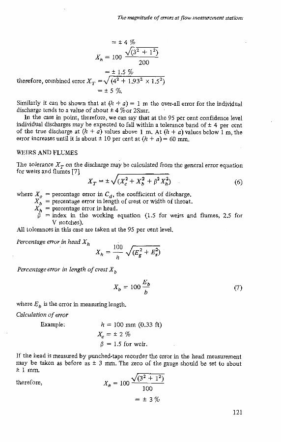
individual discharges may be expected to fall within a tolerance band of k 4 per cent of the true discharge at (h + a) values above 1 m. At (h + a) values below 1 m, the error increases until it is about f 10 per cent at (h + a) = 60 mm. WEIRS AND FLUMES The tolerance X, on the discharge may be calculated from the general error equation for weirs and flumes [7]

x, = k J(X,’ + x,2 + p’x,”> (6)

where X, = percentage error in C,, the coefficient of discharge. X, = percentage error in length of crest or width of throat. X, = percentage error in head. p = index in the working equation (1.5 for weirs and flumes, 2.5 for

V not ches). All tolerances in this case are taken at the 95 per cent level.

Percentage error in head X,

h

Percentage error in length of crest X,

x, = 100- b

where E, is the error in measuring length. Calculation of error

Example : h = 100 mm (0.33 ft)

/3 = 1.5 for weir. Xc=f2%

If the head is measured by punched-tape recorder the error in the head measurement may be taken as before as k 3 mm. The zero of the gauge should be set to about k 1 mm.

therefore, 4 3 2 $. 12) x, = 100 100

121

R. W. Herschy

The length of crest can reasonably be measured to about 3 mm in 3 m

therefore, 100 x 3 3 O00

x, = ~

= f 0.10 %. therefore, combined error in discharge

x, = f dix; + x; 4- B2Xi) = f J(2’ f 0.10’ 4- 1.52 X 3’)

Note: Recommended values for percentage errors in coefficients of discharge for weirs and flumes may be found in reference 7.

PRECISION OF THE DAILY MEAN DISCHARGE

The over-all or combined error considered so far has been in connexion with a single determination of discharge for any given stage. The daily mean discharge however is computed from several discharges over a period of 24 hours and its precision should be better than that for a single discharge. At a station equipped with a punched tape recorder the daily mean discharge is normally calculated from the arithmetic average of 96 fifteen-minute values of discharge. Now if these values of discharge can be treated as independent variables whose relative errors Xi, at 95 per cent confidence limits are known, then

and

where e is the average of n values of discharge Qj, Xi is the error in Qi, and XQ is the error in the daily mean discharge.

Therefore,

(10) 2 2 [QjlQ Xi12 x- = Q n2

Note, equation 10 may be simplified to the following approximation:

and if all the values Qi are equal, i.e. no fluctuation in stage, then

Xi xQ =z*

122

The magnitude of errors at flow measurement stations

REFERENCES / REFERENCES

1. International Organization for Standardization (ISO). R. 748. 1969.

2. International Organization for Standardization (ISO). R. 1100. 1969. Velocity Area Methods. Geneva.

Establishment and Operation of a Gauging Station and Determination of the Stage Discharge Relation. Geneva.

Proc. A.S.C.E., vol. 89, no. HY4.

I.C.E. Scottish Hydrological Group.

necessary? Proc. A.S.C.E., vol. 94, paper 5848.

Water Resources Board. Technical Note No. 11.

Flumes. Part 4B: Long Based (Broad-crested) Weirs.

3. Carter, R. W.; Anderson, I. E. 1963. Accuracy of current meter measurements.

4. Lambie, J. C. 1966. The Rating and Behaviour of a Group of Current Meters.

5. Smoot, G. F.; and Carter, R. W. 1968. Are individual current meter ratings

6. Herschy, R. W. 1969. The Evaluation of Errors at Flow Measurement Stations.

7. British Standard 3680 Part 4A, 1964 and Part 4B, 1969. Part4A: Thin Plate Weirs and

BIBLIOGRAPHY /BIBLIOGRAPHIE

Young, H. D. 1962. Statistical Treatment of Experimental Data. New York, Mc Graw-Hill Book

Hool, Paul G. 1963. Elementary Statistics. New York, John Wiley and Sons. Simon, L. E. 1941. A n Engineer’s Manual of Statistical Methcds. New York, John Wiley and

Mills, F. C. 1940. StatisticalMethods. New York, Henry Holt and Company. Chambers, E. G. 1958. Statistical Calculation. Cambridge University Press. British Standard 2846.

Langley, R. 1969. Practical Statistics. London. Pan Piper. Moroney, M. J. 1963. Facts from Figures. Harmondsworth, Penguin Books Ltd. Yeomans, K. A. 1968. Applied Statistics, Volumes 1 and 2. Harmondsworth. Penguin Books Ltd. Topping J. 1968. Errors of Observation and their Treatment. (Institute of Physics), London.

International Organization for Standardization. Recommendation No. 1438. Liquide H O W

International Organization for Standardization. Recommendation R. 772. 1968. Vocabulary of

Company Inc.

Sons.

1957. The Reduction and Presentation of Experimental Results.

Chapman and Hall Ltd.

Measurement in open Channels Using Thin Plate Weirs and Venturi Flumes. (Draft.).

Terms and Symbols. Geneva.

ACKNOWLEDGEMENT

The author is indebted to the Water. Resources Board (United Kingdom) for permis- sion to publish this paper.

123

R. W. Herschy

APPENDIX: DEFINITIONS OF STATISTICAL TERMS

Normal distribution

Known also as the error law, the Gaussian law, the probability curve. In such a distribution the dispersion of the individuals, or items, about the average is measured in standard deviations and 68 per cent (actually 68.27) of the individuals lie within one standard deviation of the mean, 95 per cent (actually 95.45) lie within two standGd deviations, and almost all (actually 99.73 per cent) lie within three standard deviations of the mean.

Standard deviation (s)

The standard deviation is a measure of the scatter of the items about the arithmetic mean of the sample. It is sometimes referred to as the root mean square of the deviations:

s=J- W 2 N- 1

where x = the deviation of the item from the arithmetic mean (2) or x = X - X

N = number of items.

Standard error of estimate (Se)

Also known as the “standard error”, it is a measure of the variation or “scatter” of the points about the line of average relationship. It is similar to standard deviation except that the curve of relationship takes the place of the arithmetic mean.

where d = deviation of the actual values from the computed values taken from the curve. In the case of a stage discharge curve the “d” values are the difference between the discharge,

as given from the curve, and the corresponding gauged discharge at the same stage. Dispersion can be measured in the same way as for standard deviation and if the distribution is normal, lines drawn at a vertical distance of one standard error of estimate above and below the line of regression and’ parallel to it will include about 68 per cent of the points. Parallel lines at two standard errors of estimate above and below the line of regression will include 95 per cent of the points, and lines drawn at three standard errors of estimate will include 99.73 per cent of the points.

Standard error of the mean relationship (Smr)

Also known as the “standard error of the mean”, it is a measure of the probable accuracy of the computed mean relationship

se

In the case of a stage discharge curve, Smr indicates the probable accuracy of discharges picked off the curve from corresponding stages (i.e. the rating table discharges).

The Smr tolerance band is therefore much narrower than the Se band the latter which refers to the individual items and the band within which the individual items may be expected to fall. In a stage discharge curve these individual items may be gaugings or check gaugings.

124

The magnitude of errors at flow measurement stations

Variances

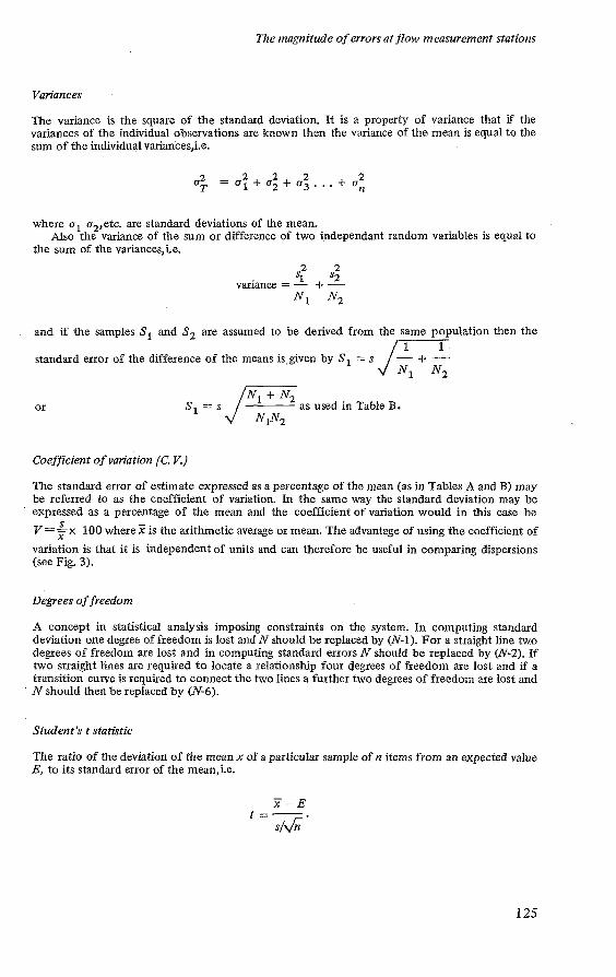
The variance is the square of the standard deviation. It is a property of variance that if the variances of the individual observations are known then the variance of the mean is equal to the sum of the individual variances,i.e.

2 T =o:+o;+0; . . . + a n

where al 02,etc. are standard deviations of the mean.

the sum of the variances,i.e. Also the variance of the sum or difference of two independant random variables is equal to

and if the samples S1 and S, are assumed to be derived from the same population then the / 1 1

standard error of the difference of the means is,given by S, = s - + - J N 1 Nz

or S, = s jG as used in Table B. NIN2

Coefficient of variation (C. V.)

The standard error of estimate expressed as a percentage of the mean (as in Tables A and €3) may be referred to as the coefficient of variation. In the same way the standard deviation may be expressed as a percentage of the mean and the coefficient of variation would in this case be V=&x 100 where? is thc arithmetic average or mean. The advantage of using the coefficient of variation is that it is independent of units and can therefore be useful in comparing dispersions (see Fig. 3).

X

Degrees of freedom

A concept in statistical analysis imposing constraints on the system. In computing standard deviation one degree of freedom is lost and N should be replaced by (N-1). For a straight line two degrees of freedom are lost and ín computing standard errors N should be replaced by (N-2). If two straight lines are required to locate a relationship four degrees of freedom are lost and if a transition curve is required to connect the two lines a further two degrees of freedom are lost and

- N should then be replaced by (N-6).

Student's t statistic

The ratio of the deviation of the mean x of a particular sample of n items from an expected value E, to its standard error of the mean,i.e.

2- E =- S I G '

125

R. W. Herschy

In the case of two means the expression becomes - - x1- x2

:I& t=-

where x1 and f2 are the means of the two samples. Note that in Table B the standard deviation of the combined observations is

NI i- N2 - -

. where (xl - XI) and (x2 - Fz) = (d, - dl) and f = d/S where 2 is difference between the check gaugings and the

rating equation and S, =

Tolerance

The tolerance on a measurement may be defined statistically as the band width around the calculated value, which, on an average of 19 times out of 20, can be expected to include the true value. The tolerance can be taken to equal approximately twice the standard deviation.

N.E. More precise definitions may be obtained from text books on mathematical statistics but it is suggested that the above definitions are suitable for application to hydrometry.

126

The magnitude of errors at flow measurement stations

NOTATION FOR TABLES A AND B

d - The percentage deviation of a measured discharge used in the construction of the rating equation from the value given by the rating equation for the corresponding gauge height.

dl - The percentage deviation of a check measurement of discharge from the value given by the - rating equation for the corresponding gauge height. dl - The arithmetic mean of the deviations (dl) of a series of check measurements of discharge;

also, assuming the rating equation represents the best mean of the original observations, the difference between that and the mean of the check observations.

N - The number of observations used in constructing the rating equation. N1 - The number of check observations. Se - Standard error of estimate. Smr - Standard error of the mean relationship. s - The best estimate of Standard Deviation of the Population of all the discharge measure- S1 - The standard error of the difference between the means of the two arrays. t e - A statistic to test the significance of the difference between the sample mean and its

ments.

hypothetical value based on Student’s distribution.

Table A - Percentage variation of actual gaugings from discharge shown by rating equation

- d2 or

Q2 - x 100

(dl - ZII2 dl - dl QI Date No. Gauge pz Rating Q2 - Ql QI height Gauging equation

=dordl

Discharge 3.3.59 4.4.59 4.4.59 16.5.59 8.6.59 12.8.59 3.9.59 21.9.59 22.9.59 22.9.59 22.9.59 22.9.59 N =

curve 1 0.95 65 2 1.45 177 3 1.35 159 4 0.90 63 5 0.80 49 6 1.90 341 7 0.90 61 8 1.10 114 9 1.35 172 10 1.45 202 11 1.55 225 12 1.62 255 12

Check gaugings -1959-60 4.12.59 13 0.95 70 12.2.60 14 1.50 220 21.3.60 15 1.10 105 N1= 3

Check gaugings - 1960-61 20.10.60 16 1.00 92 16.2.61 17 0.90 72 27.2.61 18 1.25 145 N l = 3

72.4 193 165 63.1 46.9

63.1 349

102 165 193 224 247

72.4 208 102

81.6 63.1 138

- 7.4 - 16 - 6 - 0.1

2.1 - 8 - 2.1 12 7 9 1 8

- 10.2 - 8.3 - 3.6

4.4 - 2.3 - 3.3 11.7 4.3 4.6 O .4 3.2

-

- 2.4 - 3.3 12 5.8 3 2.9

d l = 1.8 Z d l = 5.4

10.4 12.7 8.9 14.1 7.0 5-1

x d l = 31.9 dl = 10.6

104 68.9 13

19.4 5.3 10.9

18.5 21.2 0.2 10.2

Ed2 = 408.6

-

137

- 5.1 26 4.0 16

2.1 4.4 3.5 12.3

- 5.5 30.3 z(dl - dl)2 = 47

127

R. W. Herschy

Table E - Standard error of estimate. Standard error of mean. Test of check gaugings for bias

Se and Smr

Range of h = 0.80 to 1.90 ECd2(from Table A) = 408.6 N = 12 N - 2 = 10

E- = 41 d2

N - 2

Se = J"' = 6.4 76 N - 2

1959-60 check gaugings

Test of check gaugings for bias

N, = 3, 2, = 1.8, x(dl - = 43.2

s, = s = 3.8

t = dl/S1 = 1.813.8 = 0.47 For (N + N, - 2) degrees of freedom (i.e. 13) = 1.77 > 0.47

(Table C)

.. Action required None

1960-61 check gaugings

NI = 3, al = 10.6, x(dl - d1)2 = 47.0

= 5.9 N + N 1 - 2

= 3.8

t = zl/S1 = 10.613.8 = 2.79 For (N + N, - 2) degrees of freedom (Le. 13) toalo = 1.77 < 2.79

:. Action required further checks, poss. re-cali1

128

The magnitude of errors at flow measurement stations

Table C - Values of

t. Deg. freedom t; Deg .

freedom f Deg. freedom

1 6,31 11 1.80 21 1.72 2 2.92 12 1.78 22 1.72 3 2.35 13 1.77 23 1.71 4 2.13 14 1.76 24 1.7 1 5 2.02 15 1.75 25 1.7 1 6 1.94 16 1.75 26 1.7 1 7 1.90 17 1.74 27 1.10 8 1.86 18 1.73 28 ‘ 1.70 9 1.83 19 1.73 29 1.70 10 1.81 20 1.73 30 1.10

(Abridged from Table III of Statistical Tables for Biological, Agricultural and Medical Research by R.A. Fisher and F. Yates. Edinburgh, Oliver and Boyd.)

Table D

QI - Q2 Ql

Stage Gauged Q! QI 7 QZ x 100 Deviation Ratmg

Q2

b e r cent) “/SI (m) flow equation

“1s) “/s)

3.765 3.284 3.296 3.254 3.234 3.247 3.310 3.221 3.260 3.243 2.827 2.778 2.322 2.170 2.095 2.000 2.012 1.906 1.938 1.888 1.908 1.844 1.869 1.870 1.820 1.638 1.535 1.526 1.376

320.000 277.000 276.000 273.000 272.000 271.000 270.000 270.000 268.000 267.000 223.000 220.000 171.000 160.000 15 O. O00 141.000 133.000 130.000 129.000 127.000 127.000 127.000 126.000 120.000 119.000 10.7.000 95.900 94.600 88300

328.979 27 2.47 2 273.842 269.055 266.784 268.259 275.444 265.311 269.737 267.805 221.856 216.617 169.723 154.874 147.700 138.760 139.880 130.082 133.017 128.439 130.264 124.45 O 126.712 126.803 122.290 106.289 97.537 96.783 84.481

8.979 - 4.528 - 2.158 - 3.945 - 5.216 - 2.741 5.444 - 4.689 1.737 0.805

- 1.144 - 3.383 - 1.277 - 5.126 - 2.300 - 2.240 6.880 0.082 4.017 1.439 3.264

0.712 6.80 3 3.290

1.637 2.183

- 2550

- 0.711

- 3.819

3 -2 - 1 - 1 -2 - 1 2

- 2 1 0

- 1 - 2 - 1 - 3 - 2 -2 5 0 3 1 3

- 2 1 5 3

- 1 2 2

-5 continued overleaf

3 29

R. W. Herschy

Table D

QI - Q2 QI QI 7 Q2 x 100 Deviation Ql

Rating Q2

Stage Gauged

(m3/s) (per cent) (4 flow equation

(m3/s) (m31s)

1.376 87.200 84.481 - 2.719 - 3 1.350 81.100 82.400 - 1.300 2 1.154 67.400 67.229 - 0.171 0 1.166 66.900 68.130 1.230 2 1.137 65.400 65.957 0.557 1 1.006 58.800 56.408 - 2.392 -4 0.968 55.600 53.723 - 1.877 -3 0.930 53.000 51.078 - 1.922 -4 0.916 51.400 50.113 - 1.287 - 3 0.893 47.300 48.541 1.241 3 0.808 42.900 42.863 - 0.037 0 0.781 42.700 41.104 - 1.596 -4 0.803 41.100 42.536 1.436 3 0.764 39.300 40.009 0.709 2 0.731 38.400 37.907 - 0.493 - 1 0.709 37.300 36.525 - 0.775 - 2 0.706 36.600 36.337 - 0.263 - 1 0.710 36.000 36.587 0.587 2 0.676 32.400 34.481 2.081 6 0.549 26.600 26.955 0.355 1 . 0.483 23.600 23.27 1 - 0.329 - 1 0.437 20.700 20.802 0.102 0 0.425 20.500 20.172 - 0.328 - 2 0.408 19.100 19.289 0.189 1 0.385 18.200 18.113 - 0.087 0 0.383 17.900 18.012 0.112 1

Summary: The line that gives the best estimate of Q, for a given H, with approx 95 per cent confidence limits is given by

log (Q) = log (C) + Q: log (H + A) f E between thelimits 0.383 and 3.765 where log C - 3.8555, A = 0.13, (Y = 1.428 E = i 5 and C = 47.25 and Q = 47.25 (H + 0.13)1.428.

DISCUSSION

Smoot: I have to comment on the table conceming the errors. In the United States we have run some extensive tests on the calibration of current meters by groups or individually. Our experience would indicate that our group ratings are equally as accurate as individual ratings and we have approximately the same standard for either as Mr. Herschy lists for the individual ratings. This is a matter of quality control. We have calibrated 10 per cent of our meters which amounted to 227 calibrations this year. We are now analysing these calibrations. The results indicate standard errors of approximately twodthirds the value mentioned here, resulting from tightening of the manufacturing of the current meters.

130

The magnitude of errors at flow measurement stations

Garg: In india, we are measuring discharges on large rivers carrying discharges to about 60 O00 m3/sec. Have errors in higher ranges, say for discharges of about 3,000 m3/sec. occurred and what is the percentage of error?

Herschy: Errors at lower discharges are generally higher than errors at the higher discharges, within reasonable limits of course.

Wartena: The number of verticals must increase with increasing width of the stream. Did you neglect this tendency, which is not linear.

Herschy: The largest component of the error is certain1.y emerging from the verticals. The number of verticals reduces the errors.

Wartena: I wanted to point out the number of verticals has to increase with the width of the stream, but not proportionally. How did you bring this into calculation? i understood that you neglected this.

Herschy: No, this is included in equation 1. The tables show a number of verticals with the error for these verticals.

Wartena: Yes, but that must depend on the dimension length schedule?

Herschy: Yes.

131