NBER WORKING PAPER SERIES

THE MACROECONOMICS OF EPIDEMICS

Martin S. EichenbaumSergio Rebelo

Mathias Trabandt

Working Paper 26882http://www.nber.org/papers/w26882

NATIONAL BUREAU OF ECONOMIC RESEARCH1050 Massachusetts Avenue

Cambridge, MA 02138March 2020, Revised April 2020

We are grateful to Andy Atkeson, Gadi Barlevy, Francisco Ciocchini, Warren Cornwall, Ana Cusolito, João Guerreiro, Ravi Jaganathan, Aart Kraay, Michael King, Per Krusell, Chuck Manski, Paul Romer, Alp Simsek, and Steve Strongin for their comments. We thank Bence Bardoczy and Laura Murphy for excellent research assistance. The views expressed herein are those of the authors and do not necessarily reflect the views of the National Bureau of Economic Research.

NBER working papers are circulated for discussion and comment purposes. They have not been peer-reviewed or been subject to the review by the NBER Board of Directors that accompanies official NBER publications.

© 2020 by Martin S. Eichenbaum, Sergio Rebelo, and Mathias Trabandt. All rights reserved. Short sections of text, not to exceed two paragraphs, may be quoted without explicit permission provided that full credit, including © notice, is given to the source.

The Macroeconomics of EpidemicsMartin S. Eichenbaum, Sergio Rebelo, and Mathias Trabandt NBER Working Paper No. 26882March 2020, Revised April 2020JEL No. E1,H0,I1

ABSTRACT

We extend the canonical epidemiology model to study the interaction between economic decisions and epidemics. Our model implies that people’s decision to cut back on consumption and work reduces the severity of the epidemic, as measured by total deaths. These decisions exacerbate the size of the recession caused by the epidemic. The competitive equilibrium is not socially optimal because infected people do not fully internalize the effect of their economic decisions on the spread of the virus. In our benchmark model, the best simple containment policy increases the severity of the recession but saves roughly half a million lives in the U.S.

Martin S. EichenbaumDepartment of EconomicsNorthwestern University2003 Sheridan RoadEvanston, IL 60208and NBEReich@northwestern.edu

Sergio RebeloNorthwestern UniversityKellogg School of ManagementDepartment of FinanceLeverone HallEvanston, IL 60208-2001and CEPRand also NBERs-rebelo@northwestern.edu

Mathias TrabandtFreie Universität BerlinSchool of Business and EconomicsBoltzmannstrasse 2014195 BerlinGermanyand DIW and IWHmathias.trabandt@gmail.com

The Macroeconomics of Epidemics!y

Martin S. Eichenbaumz Sergio Rebelox Mathias Trabandt{

April 10, 2020

Abstract

We extend the canonical epidemiology model to study the interaction between eco-nomic decisions and epidemics. Our model implies that peopleís decision to cut backon consumption and work reduces the severity of the epidemic, as measured by totaldeaths. These decisions exacerbate the size of the recession caused by the epidemic.The competitive equilibrium is not socially optimal because infected people do notfully internalize the e§ect of their economic decisions on the spread of the virus. Inour benchmark model, the best simple containment policy increases the severity of therecession but saves roughly half a million lives in the U.S.

JEL ClassiÖcation: E1, I1, H0Keywords: Epidemic, COVID-19, recessions, vaccine, containment policies, smart

containment, early exit, late start, SIR macro model.

!We are grateful to Andy Atkeson, Gadi Barlevy, Francisco Ciocchini, Warren Cornwall, Ana Cusolito,Jo„o Guerreiro, Ravi Jaganathan, Aart Kraay, Michael King, Per Krusell, Chuck Manski, Paul Romer, AlpSimsek, and Steve Strongin for their comments. We thank Bence Bardoczy and Laura Murphy for excellentresearch assistance.

yMatlab replication codes can be downloaded from the authorsí websites or directly from the URL:https://tinyurl.com/ERTcode

zNorthwestern University and NBER. Address: Northwestern University, Department of Economics, 2211Campus Dr, Evanston, IL 60208. USA. E-mail: eich@northwestern.edu.

xNorthwestern University, NBER, and CEPR. Address: Northwestern University, Kellogg School of Man-agement, 2211 Campus Dr, Evanston, IL 60208. USA. E-mail: s-rebelo@kellogg.northwestern.edu.

{Freie Universit‰t Berlin, School of Business and Economics, Chair of Macroeconomics. Address: Boltz-mannstrasse 20, 14195 Berlin, Germany, German Institute for Economic Research (DIW) and Halle Institutefor Economic Research (IWH), E-mail: mathias.trabandt@gmail.com.

1 Introduction

As COVID-19 spreads throughout the world, governments are struggling with how to un-

derstand and manage the epidemic. Epidemiology models have been widely used to predict

the course of the epidemic (e.g., Ferguson et al. (2020)). While these models are very use-

ful, they do have an important shortcoming: they do not allow for the interaction between

economic decisions and rates of infection.

Policy makers certainly appreciate this interaction. For example, in their March 19, 2020

Financial Times op-ed Ben Bernanke and Janet Yellen write that

"In the near term, public health objectives necessitate people staying home from

shopping and work, especially if they are sick or at risk. So production and

spending must inevitably decline for a time."

In this paper, we extend the classic SIR model proposed by Kermack and McKendrick

(1927) to study the equilibrium interaction between economic decisions and epidemic dy-

namics.1 Our model makes clear that peopleís decisions to cut back on consumption and

work reduce the severity of the epidemic as measured by total deaths. These same decisions

exacerbate the size of the recession caused by the epidemic.

In our model, an epidemic has both aggregate demand and aggregate supply e§ects.

The supply e§ect arises because the epidemic exposes people who are working to the virus.

People react to that risk by reducing their labor supply. The demand e§ect arises because the

epidemic exposes people who are purchasing consumption goods to the virus. People react

to that risk by reducing their consumption. The supply and demand e§ects work together

to generate a large, persistent recession.

The competitive equilibrium is not Pareto optimal because people infected with the virus

do not fully internalize the e§ect of their consumption and work decisions on the spread of

the virus. To be clear, this market failure does not reáect a lack of good intentions or

irrationality on the part of infected people. It simply reáects the fact that each person takes

economy-wide infection rates as given.

A natural question is: what policies should the government pursue to deal with the

infection externality? We focus on simple containment policies that reduce consumption and

hours worked. By reducing economic interactions among people, these policies exacerbate the

1SIR is an acronym for susceptible, infected, and recovered or removed.

1

recession but raise welfare by reducing the death toll caused by the epidemic. We Önd that

it is optimal to introduce large-scale containment measures that result in a sharp, sustained

drop in aggregate output. In our benchmark model, when vaccines and treatments donít

arrive before the epidemic is over and healthcare capacity is limited, containment policy

saves roughly half-a-million lives in the U.S.

To make the intuition for our results as transparent as possible, we use a relatively simple

model. A cost of that simplicity is that we cannot study many important, epidemic-related

policy issues. For example, we do not consider polices that mitigate the economic hardships

su§ered by households and businesses. Such policies include Öscal transfers to households and

loans to keep Örms from going bankrupt. We also do not study policies aimed at maintaining

the liquidity and health of Önancial markets.

Finally, we abstract from nominal rigidities which could play an important role in de-

termining the short-run response of the economy to an epidemic. For example, if prices are

sticky, a given fall in the demand for consumption would generate a larger recession. Other

things equal, a larger recession would mitigate the spread of the infection. We plan to ad-

dress these important issues in future work. But we are conÖdent that the central message

from our current analysis will be robust: there is an inevitable trade-o§ between the severity

of the recession and the health consequences of the epidemic.2

Our point of departure is the canonical SIR model proposed by Kermack and McKendrick

(1927). In this model, the transition probabilities between health states are exogenous

parameters. We modify the model by assuming that purchasing consumption goods and

working brings people in contact with each other. These activities raise the probability that

the infection spreads. We refer to the resulting framework as the SIR-macro model.

We choose parameters so that the Kermack-McKendrick SIR model is consistent with

the scenario outlined by Angela Merkel in her March 11, 2020 speech.3 According to this

scenario, ì60 to 70 percent of the population will be infected as long as this remains the

situation.î Using 60 percent as our benchmark value, the SIR model implies that the share

of the initial population infected peaks at 6:8 percent. Applying this scenario to the U.S.

implies that roughly 200 million Americans eventually become infected and one million

people die. When we embed the SIR model in a simple general equilibrium framework

in which economic decisions do not a§ect the dynamics of the epidemic, we Önd that the

2In an interesting essay, Gourinchas (2020) makes a similar point.3"Merkel Gives Germans a Hard Truth About the Corona Virus," New York Times, March 11, 2020.

2

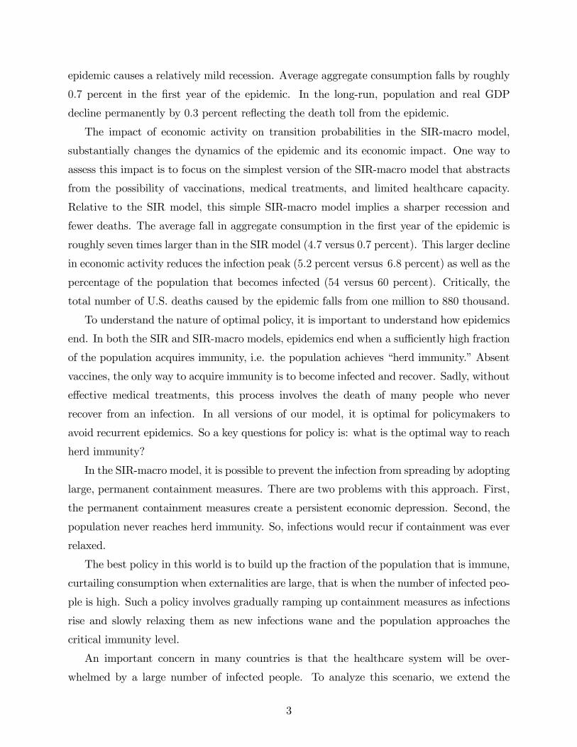
epidemic causes a relatively mild recession. Average aggregate consumption falls by roughly

0:7 percent in the Örst year of the epidemic. In the long-run, population and real GDP

decline permanently by 0:3 percent reáecting the death toll from the epidemic.

The impact of economic activity on transition probabilities in the SIR-macro model,

substantially changes the dynamics of the epidemic and its economic impact. One way to

assess this impact is to focus on the simplest version of the SIR-macro model that abstracts

from the possibility of vaccinations, medical treatments, and limited healthcare capacity.

Relative to the SIR model, this simple SIR-macro model implies a sharper recession and

fewer deaths. The average fall in aggregate consumption in the Örst year of the epidemic is

roughly seven times larger than in the SIR model (4:7 versus 0:7 percent). This larger decline

in economic activity reduces the infection peak (5:2 percent versus 6:8 percent) as well as the

percentage of the population that becomes infected (54 versus 60 percent). Critically, the

total number of U.S. deaths caused by the epidemic falls from one million to 880 thousand.

To understand the nature of optimal policy, it is important to understand how epidemics

end. In both the SIR and SIR-macro models, epidemics end when a su¢ciently high fraction

of the population acquires immunity, i.e. the population achieves ìherd immunity.î Absent

vaccines, the only way to acquire immunity is to become infected and recover. Sadly, without

e§ective medical treatments, this process involves the death of many people who never

recover from an infection. In all versions of our model, it is optimal for policymakers to

avoid recurrent epidemics. So a key questions for policy is: what is the optimal way to reach

herd immunity?

In the SIR-macro model, it is possible to prevent the infection from spreading by adopting

large, permanent containment measures. There are two problems with this approach. First,

the permanent containment measures create a persistent economic depression. Second, the

population never reaches herd immunity. So, infections would recur if containment was ever

relaxed.

The best policy in this world is to build up the fraction of the population that is immune,

curtailing consumption when externalities are large, that is when the number of infected peo-

ple is high. Such a policy involves gradually ramping up containment measures as infections

rise and slowly relaxing them as new infections wane and the population approaches the

critical immunity level.

An important concern in many countries is that the healthcare system will be over-

whelmed by a large number of infected people. To analyze this scenario, we extend the

3

simple SIR-macro model so that the mortality rate is an increasing function of the number

of people infected. We Önd that the competitive equilibrium involves a much larger reces-

sion, as people internalize the higher mortality rates. People cut back more aggressively on

consumption and work to reduce the probability of being infected. As a result, fewer people

are infected in the competitive equilibrium but more people die. The optimal policy involves

a much more aggressive response than in the simple SIR-macro economy. The reason is that

the cost of the externality is much larger since a larger fraction of the infected population

dies.

How does the possibility of an e§ective treatment being discovered change our results?

The qualitative implications are clear: people become more willing to engage in market

activities because the expected cost of being infected is smaller. So, along a path in which

treatment is not actually discovered, the recession induced by the epidemic is less severe.

Sadly, along such a path, the total number of infected people and the death toll rise relative

to the baseline SIR-macro model. That said, the quantitative di§erence of this model and the

baseline SIR-macro model is quite small, both with respect to the competitive equilibrium

and the best containment policy.

How does the possibility of a vaccine being discovered change our results? Vaccines donít

cure infected people but they do prevent susceptible people from becoming infected. In con-

trast, treatments cure infected people but do not prevent future infections. These di§erences

are not very important for the competitive equilibrium. But they are very important for

the design of optimal policy. With vaccines as a possibility, it is optimal to immediately

introduce severe containment measures to minimize deaths. Those measures cause a large

recession. But this recession is worth incurring in the hope that vaccination arrives before

many people get infected.

The most general version of our model, discussed in Section 6, incorporates the proba-

bilistic development of vaccines and treatments, as well as a mortality rate that rises with the

number of infected people. The latter feature reáects capacity constraints in the healthcare

system. We refer to this version of the model as the benchmark SIR-macro model.

In this model, it is optimal to immediately introduce severe containment measures and

increase those measures as more of the population is infected. The best containment policy

dramatically increases the magnitude of the recession. Absent containment measures, aver-

age consumption falls by about 7 percent in the Örst year of the epidemic. With optimal

containment, average consumption falls by 22 percent. Notably, the size of the recession is

4

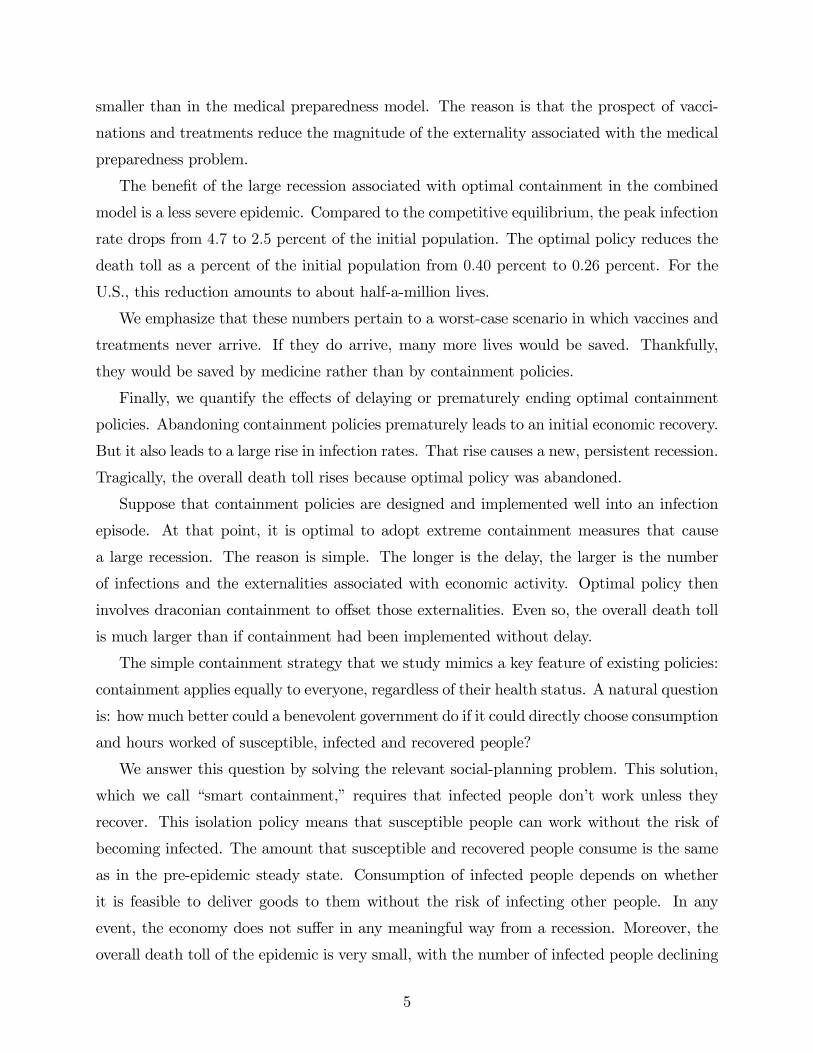
smaller than in the medical preparedness model. The reason is that the prospect of vacci-

nations and treatments reduce the magnitude of the externality associated with the medical

preparedness problem.

The beneÖt of the large recession associated with optimal containment in the combined

model is a less severe epidemic. Compared to the competitive equilibrium, the peak infection

rate drops from 4:7 to 2:5 percent of the initial population. The optimal policy reduces the

death toll as a percent of the initial population from 0:40 percent to 0:26 percent. For the

U.S., this reduction amounts to about half-a-million lives.

We emphasize that these numbers pertain to a worst-case scenario in which vaccines and

treatments never arrive. If they do arrive, many more lives would be saved. Thankfully,

they would be saved by medicine rather than by containment policies.

Finally, we quantify the e§ects of delaying or prematurely ending optimal containment

policies. Abandoning containment policies prematurely leads to an initial economic recovery.

But it also leads to a large rise in infection rates. That rise causes a new, persistent recession.

Tragically, the overall death toll rises because optimal policy was abandoned.

Suppose that containment policies are designed and implemented well into an infection

episode. At that point, it is optimal to adopt extreme containment measures that cause

a large recession. The reason is simple. The longer is the delay, the larger is the number

of infections and the externalities associated with economic activity. Optimal policy then

involves draconian containment to o§set those externalities. Even so, the overall death toll

is much larger than if containment had been implemented without delay.

The simple containment strategy that we study mimics a key feature of existing policies:

containment applies equally to everyone, regardless of their health status. A natural question

is: howmuch better could a benevolent government do if it could directly choose consumption

and hours worked of susceptible, infected and recovered people?

We answer this question by solving the relevant social-planning problem. This solution,

which we call ìsmart containment,î requires that infected people donít work unless they

recover. This isolation policy means that susceptible people can work without the risk of

becoming infected. The amount that susceptible and recovered people consume is the same

as in the pre-epidemic steady state. Consumption of infected people depends on whether

it is feasible to deliver goods to them without the risk of infecting other people. In any

event, the economy does not su§er in any meaningful way from a recession. Moreover, the

overall death toll of the epidemic is very small, with the number of infected people declining

5

monotonically from its initial level to zero.

The previous results point to the importance of antigen and antibody tests that would

allow health professionals to quickly ascertain peopleís health status. The social returns to

gathering this information and acting upon it are enormous. These actions reduce both the

death toll and the size of the economic contraction relative to the outcomes associated with

the best simple containment policy.

Our paper is organized as follows. In section 2, we describe both the SIR and the SIR-

macro model. In section 3, we describe the versions of the model that consider medical

preparedness and the possibility of e§ective treatment and vaccines being discovered. In

section 4, we discuss the properties of the competitive equilibrium in di§erent variants of our

model. In section 5, we solve the Ramsey policy problems and analyze their implications for

the containment of the spread of the virus and for economic activity. In section 6, we discuss

our quantitative results for the benchmark model. Section 7 discusses related literature.

Finally, Section 8 concludes.

2 The SIR-macro model

In this section, we describe the economy before the start of the epidemic. We then present

the SIR-macro model.

2.1 The pre-infection economy

The economy is populated by a continuum of ex-ante identical agents with measure one. Prior

to the start of the epidemic, all agents are identical and maximize the objective function:

U =1X

t=0

#tu(ct; nt).

Here # 2 (0; 1) denotes the discount factor and ct and nt denote consumption and hours

worked, respectively. For simplicity, we assume that momentary utility takes the form

u(ct; nt) = ln ct '(

2n2t .

The budget constraint of the representative agent is:

(1 + )t)ct = wtnt + 0t.

Here, wt denotes the real wage rate, )t is the tax rate on consumption, and 0t denotes

lump-sum transfers from the government. As discussed below, we think of )t as a proxy for

6

containment measures aimed at reducing social interactions. For this reason, we refer to )tas the containment rate.

The Örst-order condition for the representative-agentís problem is:

(1 + )t)(nt = c"1t wt.

There is a continuum of competitive representative Örms of unit measure that produce con-

sumption goods (Ct) using hours worked (Nt) according to the technology:

Ct = ANt.

The Örm chooses hours worked to maximize its time-t proÖts 1t:

1t = ANt ' wtNt.

The governmentís budget constraint is given by

)tct = 0t.

In equilibrium, nt = Nt and ct = Ct.

2.2 The outbreak of an epidemic

Epidemiology models generally assume that the probabilities governing the transition be-

tween di§erent states of health are exogenous with respect to economic decisions. We modify

the classic SIR model proposed by Kermack and McKendrick (1927) so that these transition

probabilities depend on peopleís economic decisions. Since purchasing consumption goods

or working brings people into contact with each other, we assume that the probability of

becoming infected depends on these activities.

The population is divided into four groups: susceptible (people who have not yet been

exposed to the disease), infected (people who contracted the disease), recovered (people

who survived the disease and acquired immunity), and deceased (people who died from the

disease). The fractions of people in these four groups are denoted by St, It, Rt and Dt,

respectively. The number of newly infected people is denoted by Tt.

Susceptible people can become infected in three ways. First, they can meet infected peo-

ple while purchasing consumption goods. The number of newly infected people that results

from these interactions is given by 41(StCSt )"ItC

It

#. The terms StCSt and ItC

It represent

7

total consumption expenditures by susceptible and infected people, respectively. The para-

meter 41 reáects both the amount of time spent shopping and the probability of becoming

infected as a result of that activity. In reality, di§erent types of consumption involve di§erent

amounts of contact with other people. For example, attending a rock concert is much more

contact intensive than going to a grocery store. For simplicity we abstract from this type of

heterogeneity.

Second, susceptible and infected people can meet at work. The number of newly infected

people that results from interactions at work is given by 42(StNSt )"ItN

It

#. The terms StNS

t

and ItN It represent total hours worked by susceptible and infected people, respectively. The

parameter 42 reáects the probability of becoming infected as a result of work interactions. We

recognize that di§erent jobs require di§erent amounts of contact with people. For example,

working as a dentist or a waiter is much more contact intensive than writing software. Again,

for simplicity, we abstract from this source of heterogeneity.

Third, susceptible and infected people can meet in ways not directly related to consuming

or working, for example meeting a neighbor or touching a contaminated surface. The number

of random meetings between infected and susceptible people is StIt. These meetings result

in 43StIt newly infected people.

The total number of newly infected people is given by:

Tt = 41 (StCst )"ItC

it

#+ 42 (StN

st )"ItN

it

#+ 43StIt. (1)

Kermack and McKendrickís (1927) SIR model is a special case of our model in which the

propagation of the disease is unrelated to economic activity (41 = 0, 42 = 0).

The number of susceptible people at time t + 1 is equal to the number of susceptible

people at time t minus the number of susceptible people that got infected at time t:

St+1 = St ' Tt. (2)

The number of infected people at time t + 1 is equal to the number of infected people

at time t plus the number of newly infected (Tt) minus the number infected people that

recovered (4rIt) and the number of infected people that died (4dIt):

It+1 = It + Tt ' (4r + 4d) It. (3)

Here, 4r is the rate at which infected people recover from the infection and 4d is the mortality

rate, that is the probability that an infected person dies.

8

The timing convention implicit in equation (3) is as follows. Social interactions happen in

the beginning of the period (infected and susceptible people meet). Then, changes in health

status unrelated to social interactions (recovery or death) occur. At the end of the period,

the consequences of social interactions materialize: Tt susceptible people become infected.

The number of recovered people at time t+ 1 is the number of recovered people at time

t plus the number of infected people who just recovered (4rIt):

Rt+1 = Rt + 4rIt. (4)

Finally, the number of deceased people at time t + 1 is the number of deceased people at

time t plus the number of new deaths (4dIt):

Dt+1 = Dt + 4dIt. (5)

Total population, Popt+1, evolves according to:

Popt+1 = Popt ' 4dIt,

with Pop0 = 1.

We assume that at time zero, a fraction " of susceptible people is infected by a virus

through zoonotic exposure, that is the virus is directly transmitted from animals to humans,

I0 = ",

S0 = 1' ".

Everybody is aware of the initial infection and understand the laws of motion governing

population health dynamics. Critically, they take as given aggregate variables like ItCIt and

ItNIt .

We now describe the optimization problem of di§erent types of people in the economy.

The variable U jt denotes the time-t lifetime utility of a type-j agent (j = s; i; r). The budget

constraint of a type-j person is

(1 + )t)cjt = wt=

jnjt + 0t, (6)

where cjt and njt denote the consumption and hours worker of agent j, respectively. The

parameter governing labor productivity, =j, is equal to one for susceptible and recovered

people (=s = =r = 1) and less than one for infected people (=i < 1).

9

The budget constraint (6) embodies the assumption that there is no way for agents to pool

risk associated with the infection. Going to the opposite extreme and assuming complete

markets considerably complicates the analysis without necessarily making the model more

realistic.

Susceptible people The lifetime utility of a susceptible person, U st , is

U st = u(cst ; n

st) + #

$(1' ? t)U st+1 + ? tU

it+1

%. (7)

Here, the variable ? t represents the probability that a susceptible person becomes infected:

? t = 41cst

"ItC

It

#+ 42n

st

"ItN

It

#+ 43It. (8)

Critically, susceptible people understand that consuming and working less reduces the prob-

ability of becoming infected.

The Örst-order conditions for consumption and hours worked are:

u1(cst ; n

st)' (1 + )t)@

sbt + @*t41

"ItC

It

#= 0,

u2(cst ; n

st) + wt@

sbt + @*t42

"ItN

It

#= 0.

Here, @sbt and @*t are the Lagrange multipliers associated with constraints (6) and (8), re-

spectively.

The Örst-order condition for ? t is:

#"U it+1 ' U

st+1

#' @*t = 0. (9)

Infected people The lifetime utility of an infected person, U it , is

U it = u(cit; n

it) + #

$(1' 4r ' 4d)U it+1 + 4rU

rt+1

%. (10)

The expression for U it embodies a common assumption in macro and health economics that

the cost of death is the foregone utility of life.

The Örst-order conditions for consumption and hours worked are given by

u1(cit; n

it) = @

ibt(1 + )t),

u2(cit; n

it) = '=

iwt@ibt,

where @ibt is the Lagrange multiplier associated with constraint (6).

10

Recovered people The lifetime utility of a recovered person, U rt , is

U rt = u(crt ; n

rt ) + #U

rt+1. (11)

The Örst-order conditions for consumption and hours worked are:

u1(crt ; n

rt ) = @

rbt(1 + )t)

u2(crt ; n

rt ) = 'wt@

rbt

where @rbt is the Lagrange multiplier associated with constraint (6).

Government budget constraint The government budget constraint is

)t"Stc

st + Itc

it +Rtc

rt

#= 0t (St + It +Rt) .

Equilibrium In equilibrium, each person solves their maximization problem and the gov-

ernment budget constraint is satisÖed. In addition, the goods and labor markets clear:

StCst + ItC

it +RtC

rt = ANt,

StNst + ItN

it=i +RtN

rt = Nt.

In the appendix, we describe our algorithm for computing the equilibrium.4

3 Medical preparedness, treatments and vaccines

In this section, we extend the SIR-macro model in three ways. First, we allow for the

possibility that the mortality rate increases as the number of infections rises. Second, we

allow for the probabilistic development of a cure for the disease. Third, we allow for the

probabilistic development of a vaccine that inoculates susceptible people against the virus.

3.1 The medical preparedness model

In our basic SIR-macro model we abstracted from the possibility that the e¢cacy of the

healthcare system will deteriorate if a substantial fraction of the population becomes infected.

4Matlab replication codes can be downloaded from the authorsí websites or directly from the URL:https://tinyurl.com/ERTcode

11

A simple way to model this scenario is to assume that the mortality rate depends on the

number of infected people, It:

4dt = 4d + AI2t .

This functional form implies that the mortality rate is a convex function of the fraction of

the population that becomes infected. The basic SIR-macro corresponds to the special case

of A = 0.

3.2 The treatment model

The basic SIR-macro model abstracts from the possibility that an e§ective treatment against

the virus will be developed. Suppose instead that an e§ective treatment that cures infected

people is discovered with probability Bc each period. Once discovered, treatment is provided

to all infected people in the period of discovery and all subsequent periods transforming

them into recovered people. As a result, the number of new deaths from the disease goes to

zero.

The lifetime utility of an infected person before the treatment becomes available is:

U it = u(cit; n

it) + (1' Bc)

$(1' 4r ' 4d) #U it+1 + 4r#U

rt+1

%+ #BcU

rt+1. (12)

This expression reáects the fact that with probability 1' Bc a person who is infected at time

t remains so at time t+ 1. With probability Bc this person receives treatment and becomes

recovered.

We now discuss the impact of an e§ective treatment on population dynamics. Before

the treatment is discovered, population dynamics evolve according to equations (1), (2), (3),

(4), and (5). Suppose that the treatment is discovered at the beginning of time t#. Then,

all infected people become recovered. The number of deceased stabilizes once the treatment

arrives:

Dt = Dt! for t ( t#.

Since anyone can be instantly cured, we normalize the number of susceptible and infected

people to zero for t > t#. The number of recovered people is given by

Rt = 1'Dt.

12

3.3 The vaccination model

The basic SIR-macro model abstracts from the possibility that a vaccine against the virus

will be developed. Suppose instead that a vaccine is discovered with probability Bv per

period. Once discovered, the vaccine is provided to all susceptible people in the period of

discovery and in all subsequent periods.

The lifetime utility of a susceptible person is given by

U st = u(cst ; n

st) + (1' Bv)

$(1' ? t) #U st+1 + ? t#U

it+1

%+ Bv#U

rt+1. (13)

This expression reáects the fact that with probability 1' Bv a person who is susceptible at

time t remains so at time t+ 1. With probability Bv this person is vaccinated and becomes

immune to the disease. So, at time t+1, this personís health situation is identical to that of a

recovered person. The vaccine has no impact on people who were infected or have recovered.

The lifetime utilities of infected and recovered people person are given by (10) and (11),

respectively.

We now discuss the impact of vaccinations on population dynamics. Before the vaccine is

discovered, these dynamics evolve according to equations (1), (2), (3), (4), and (5). Suppose

that the vaccine is discovered at the beginning of time t#. Then, all susceptible people

become recovered. Since no one is susceptible, there are no new infections.

Denote the number of susceptible and recovered people right after a vaccine is introduced

at time t# by S 0t! and R0t! . The value of these variables are

S 0t! = 0

R0t! = Rt! + St! :

For t ( t# we have

Rt+1 =

&R0t + 4rItRt + 4rIt

for t = t#

for t > t#:

The laws of motion for It and Dt are given by (3) and (5).

4 Competitive equilibrium

In this section, we discuss the properties of the competitive equilibrium via a series of nu-

merical exercises. In the Örst subsection, we describe our parameter values. In the second

13

and third subsections, we discuss how the economy responds to an epidemic in the SIR

and SIR-macro models, respectively. In the fourth subsection, we discuss the implications

of medical preparedness. In the Öfth subsection, we discuss the e§ects of treatments and

vaccines. Finally, in the sixth subsection we discuss the robustness of our results.

4.1 Parameter values

Below, we report our choice of parameters. We are conscious that there is considerable

uncertainty about the true values of these parameters. Below, we report robustness of our

results to parameter conÖgurations.

Each time period corresponds to a week. To choose the mortality rate, 4d, we use

data from the South Korean Ministry of Health and Welfare from March 16, 2020.5 These

estimates are relatively reliable because, as of late March, South Korea had the worldís

highest per capita test rates for COVID-19 (Pueyo (2020)). Estimates of mortality rates

based on data from other countries are probably biased upwards because the number of

infected people is likely to be underestimated. We compute the weighted average of the

mortality rates using weights equal to the percentage of the U.S. population for di§erent age

groups. If we exclude people aged 70 and over, because their labor-force participation rates

is very low, we obtain an average mortality rate of 0:4 percent. If we exclude people aged

75 and over, we obtain an average mortality rate of 0:7 percent. Based on these estimates,

we set the mortality rate equal to 0:5 percent and report robustness below. As in Atkeson

(2020), we assume that it takes on average 18 days to either recover or die from the infection.

Since our model is weekly, we set 4r + 4d = 7=18. A 0:5 percent mortality rate for infected

people implies 4d = 7) 0:005=18.

We now discuss our calibration procedure to choose the values of 41, 42, and 43. It

is common in epidemiology to assume that the relative importance of di§erent modes of

transmission is similar across viruses that cause respiratory diseases. Ferguson et al. (2006)

argue that, in the case of ináuenza, 30 percent of transmissions occur in the household, 33

percent in the general community, and 37 percent occurs in schools and workplaces.

To map these estimates into our transmission parameters, we proceed as follows. We use

the Bureau of Labor Statistics 2018 Time Use Survey to estimate the percentage of time spent

on ìgeneral community activitiesî that is devoted to consumption. We compute the latter

as the fraction of time spent on ìpurchasing goods and servicesî or ìeating and drinking

5This estimate is roughly 8 times larger than the average áu death rate in the U.S.

14

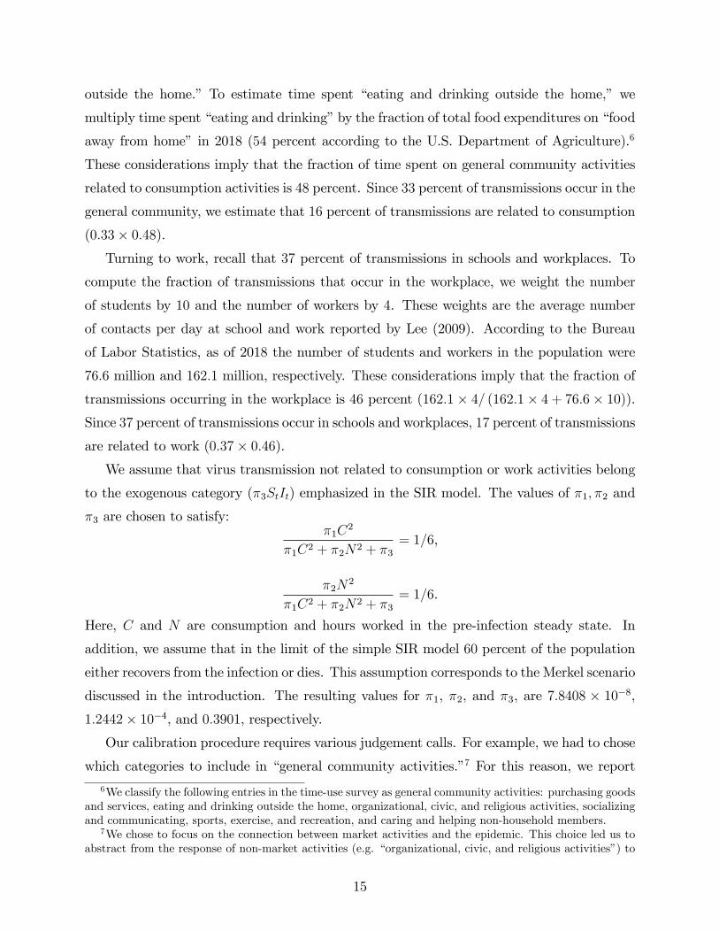
outside the home.î To estimate time spent ìeating and drinking outside the home,î we

multiply time spent ìeating and drinkingî by the fraction of total food expenditures on ìfood

away from homeî in 2018 (54 percent according to the U.S. Department of Agriculture).6

These considerations imply that the fraction of time spent on general community activities

related to consumption activities is 48 percent. Since 33 percent of transmissions occur in the

general community, we estimate that 16 percent of transmissions are related to consumption

(0:33) 0:48).

Turning to work, recall that 37 percent of transmissions in schools and workplaces. To

compute the fraction of transmissions that occur in the workplace, we weight the number

of students by 10 and the number of workers by 4. These weights are the average number

of contacts per day at school and work reported by Lee (2009). According to the Bureau

of Labor Statistics, as of 2018 the number of students and workers in the population were

76:6 million and 162:1 million, respectively. These considerations imply that the fraction of

transmissions occurring in the workplace is 46 percent (162:1) 4= (162:1) 4 + 76:6) 10)).

Since 37 percent of transmissions occur in schools and workplaces, 17 percent of transmissions

are related to work (0:37) 0:46).

We assume that virus transmission not related to consumption or work activities belong

to the exogenous category (43StIt) emphasized in the SIR model. The values of 41; 42 and

43 are chosen to satisfy:41C

2

41C2 + 42N2 + 43= 1=6,

42N2

41C2 + 42N2 + 43= 1=6.

Here, C and N are consumption and hours worked in the pre-infection steady state. In

addition, we assume that in the limit of the simple SIR model 60 percent of the population

either recovers from the infection or dies. This assumption corresponds to the Merkel scenario

discussed in the introduction. The resulting values for 41, 42, and 43, are 7:8408 ) 10"8,

1:2442) 10"4, and 0:3901, respectively.

Our calibration procedure requires various judgement calls. For example, we had to chose

which categories to include in ìgeneral community activities.î7 For this reason, we report

6We classify the following entries in the time-use survey as general community activities: purchasing goodsand services, eating and drinking outside the home, organizational, civic, and religious activities, socializingand communicating, sports, exercise, and recreation, and caring and helping non-household members.

7We chose to focus on the connection between market activities and the epidemic. This choice led us toabstract from the response of non-market activities (e.g. ìorganizational, civic, and religious activitiesî) to

15

robustness results below.

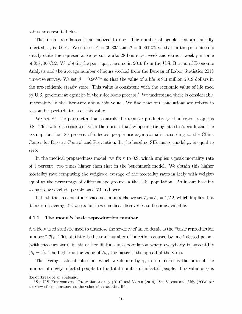
The initial population is normalized to one. The number of people that are initially

infected, ", is 0:001. We choose A = 39:835 and ( = 0:001275 so that in the pre-epidemic

steady state the representative person works 28 hours per week and earns a weekly income

of $58; 000=52. We obtain the per-capita income in 2019 from the U.S. Bureau of Economic

Analysis and the average number of hours worked from the Bureau of Labor Statistics 2018

time-use survey. We set # = 0:961=52 so that the value of a life is 9:3 million 2019 dollars in

the pre-epidemic steady state. This value is consistent with the economic value of life used

by U.S. government agencies in their decisions process.8 We understand there is considerable

uncertainty in the literature about this value. We Önd that our conclusions are robust to

reasonable perturbations of this value.

We set =i, the parameter that controls the relative productivity of infected people is

0:8. This value is consistent with the notion that symptomatic agents donít work and the

assumption that 80 percent of infected people are asymptomatic according to the China

Center for Disease Control and Prevention. In the baseline SIR-macro model )t is equal to

zero.

In the medical preparedness model, we Öx A to 0:9, which implies a peak mortality rate

of 1 percent, two times higher than that in the benchmark model. We obtain this higher

mortality rate computing the weighted average of the mortality rates in Italy with weights

equal to the percentage of di§erent age groups in the U.S. population. As in our baseline

scenario, we exclude people aged 70 and over.

In both the treatment and vaccination models, we set Bc = Bv = 1=52, which implies that

it takes on average 52 weeks for these medical discoveries to become available.

4.1.1 The modelís basic reproduction number

A widely used statistic used to diagnose the severity of an epidemic is the ìbasic reproduction

number,î R0. This statistic is the total number of infections caused by one infected person

(with measure zero) in his or her lifetime in a population where everybody is susceptible

(St = 1). The higher is the value of R0, the faster is the spread of the virus.

The average rate of infection, which we denote by E, in our model is the ratio of the

number of newly infected people to the total number of infected people. The value of E is

the outbreak of an epidemic.8See U.S. Environmental Protection Agency (2010) and Moran (2016). See Viscusi and Aldy (2003) for

a review of the literature on the value of a statistical life.

16

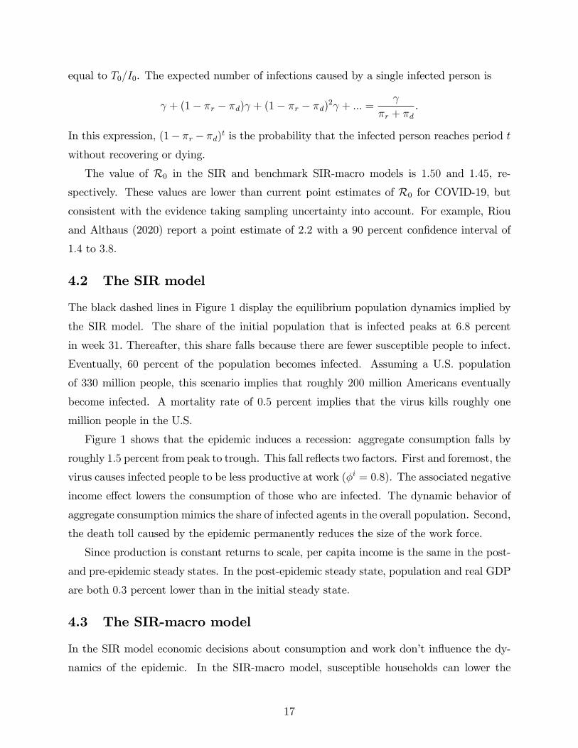
equal to T0=I0. The expected number of infections caused by a single infected person is

E + (1' 4r ' 4d)E + (1' 4r ' 4d)2E + ::: =E

4r + 4d.

In this expression, (1' 4r ' 4d)t is the probability that the infected person reaches period t

without recovering or dying.

The value of R0 in the SIR and benchmark SIR-macro models is 1:50 and 1:45, re-

spectively. These values are lower than current point estimates of R0 for COVID-19, but

consistent with the evidence taking sampling uncertainty into account. For example, Riou

and Althaus (2020) report a point estimate of 2:2 with a 90 percent conÖdence interval of

1:4 to 3:8.

4.2 The SIR model

The black dashed lines in Figure 1 display the equilibrium population dynamics implied by

the SIR model. The share of the initial population that is infected peaks at 6:8 percent

in week 31. Thereafter, this share falls because there are fewer susceptible people to infect.

Eventually, 60 percent of the population becomes infected. Assuming a U.S. population

of 330 million people, this scenario implies that roughly 200 million Americans eventually

become infected. A mortality rate of 0:5 percent implies that the virus kills roughly one

million people in the U.S.

Figure 1 shows that the epidemic induces a recession: aggregate consumption falls by

roughly 1:5 percent from peak to trough. This fall reáects two factors. First and foremost, the

virus causes infected people to be less productive at work (=i = 0:8). The associated negative

income e§ect lowers the consumption of those who are infected. The dynamic behavior of

aggregate consumption mimics the share of infected agents in the overall population. Second,

the death toll caused by the epidemic permanently reduces the size of the work force.

Since production is constant returns to scale, per capita income is the same in the post-

and pre-epidemic steady states. In the post-epidemic steady state, population and real GDP

are both 0:3 percent lower than in the initial steady state.

4.3 The SIR-macro model

In the SIR model economic decisions about consumption and work donít ináuence the dy-

namics of the epidemic. In the SIR-macro model, susceptible households can lower the

17

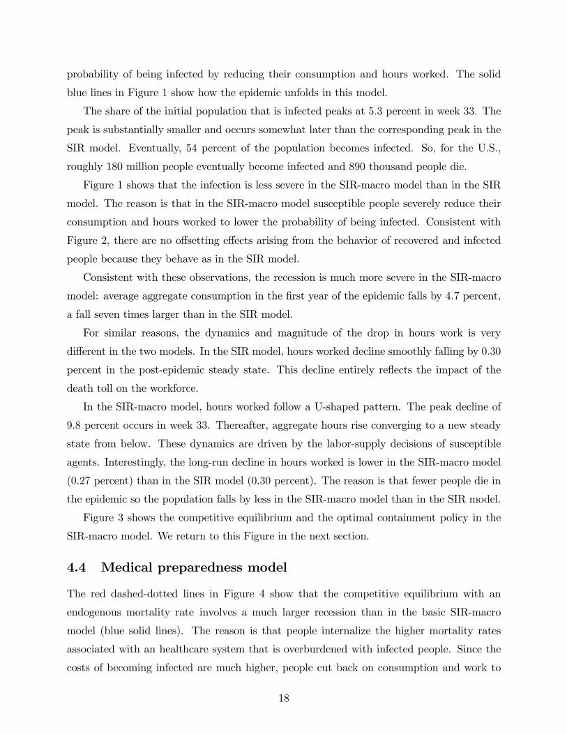
probability of being infected by reducing their consumption and hours worked. The solid

blue lines in Figure 1 show how the epidemic unfolds in this model.

The share of the initial population that is infected peaks at 5:3 percent in week 33. The

peak is substantially smaller and occurs somewhat later than the corresponding peak in the

SIR model. Eventually, 54 percent of the population becomes infected. So, for the U.S.,

roughly 180 million people eventually become infected and 890 thousand people die.

Figure 1 shows that the infection is less severe in the SIR-macro model than in the SIR

model. The reason is that in the SIR-macro model susceptible people severely reduce their

consumption and hours worked to lower the probability of being infected. Consistent with

Figure 2, there are no o§setting e§ects arising from the behavior of recovered and infected

people because they behave as in the SIR model.

Consistent with these observations, the recession is much more severe in the SIR-macro

model: average aggregate consumption in the Örst year of the epidemic falls by 4:7 percent,

a fall seven times larger than in the SIR model.

For similar reasons, the dynamics and magnitude of the drop in hours work is very

di§erent in the two models. In the SIR model, hours worked decline smoothly falling by 0:30

percent in the post-epidemic steady state. This decline entirely reáects the impact of the

death toll on the workforce.

In the SIR-macro model, hours worked follow a U-shaped pattern. The peak decline of

9:8 percent occurs in week 33. Thereafter, aggregate hours rise converging to a new steady

state from below. These dynamics are driven by the labor-supply decisions of susceptible

agents. Interestingly, the long-run decline in hours worked is lower in the SIR-macro model

(0:27 percent) than in the SIR model (0:30 percent). The reason is that fewer people die in

the epidemic so the population falls by less in the SIR-macro model than in the SIR model.

Figure 3 shows the competitive equilibrium and the optimal containment policy in the

SIR-macro model. We return to this Figure in the next section.

4.4 Medical preparedness model

The red dashed-dotted lines in Figure 4 show that the competitive equilibrium with an

endogenous mortality rate involves a much larger recession than in the basic SIR-macro

model (blue solid lines). The reason is that people internalize the higher mortality rates

associated with an healthcare system that is overburdened with infected people. Since the

costs of becoming infected are much higher, people cut back on consumption and work to

18

reduce the probability of becoming infected. The net result is that fewer people are infected

but more people die.

4.5 The treatment and vaccines models

As discussed in the introduction, the possibility of treatment and vaccination have similar

qualitative e§ects on the competitive equilibrium. Compared to the basic SIR-macro model

people become more willing to engage in market activities. The reason is that the expected

costs associated with being infected are smaller. Because of this change in behavior, the

recession is less severe. In Figures 5 and 6 the blue-solid and red-dashed-dotted lines virtually

coincide. So, in practice the quantitative e§ect of the possibility of treatments or vaccinations

on the competitive equilibrium is quite small.

4.6 Robustness

Table 1 reports the results of a series of robustness exercises where we vary key parameters

of the basic SIR-macro model. Recall that we choose our baseline parameters so that, in

the SIR model, 60 percent of the population is eventually infected by the virus. We report

results for two alternative long-run infection rates in the SIR model: 50 and 70 percent. Not

surprisingly, the higher is the long-run infection rate, the larger is the drop in consumption,

the peak infection rate, the cumulative death rate, and the total number of U.S. deaths.

Next we consider the parameter =i that controls the productivity of infected workers.

The lower is =i, the larger is the average consumption drop, the peak infection rate, the

cumulative death rate, and the total number of U.S. deaths.

Table 1 also reports the results for di§erent parameters of the infection transmission

function, (1). Recall that in the benchmark model we choose our baseline parameters so

that, in the beginning of the infection episode, economic decisions account for 1=3 of the

infection rate. Table 1 summarizes results for the case where economic decisions account for

1=6 of the initial infection rate. In this scenario, the drop in consumption is smaller. The

peak infection rate, the cumulative death rate, and the total number of U.S. deaths is larger.

These results reáect the fact that people understand that economic activity has less of an

impact on infection rates. Table 1 also reports the case in which economic decisions account

for 2=3 of the initial infection rate. In this scenario, the drop in consumption is larger. But

the peak infection rate and the cumulative death rate are smaller. These results reáect the

19

fact that people cut back more on economic activities since these activities have a larger

impact on infection rates.

Next, we increase the mortality rate from 0:5 percent to 1 percent.9 This change increases

the severity of the recession as people cut back on their consumption and work to reduce

the chances of being infected. Despite the concomitant fall in peak infection rates, the

cumulative death rate, and the number of U.S. deaths rise.

Table 1 summarizes the impact of a change in the medical-preparedness parameter, A.

The lower is A, the higher is the degree of medical preparedness. We consider a value of

A = 0:9 such that the mortality rate in the medical preparedness model peaks at 1 percent.

Table 1 shows that this higher value of A is associated with a more severe recession as people

curtail economic activity in response to higher mortality rates. While the peak level of

infections fall, the cumulative death rate and the total number of U.S. deaths rise.

Finally, we assess the impact of reducing the discount factor from 0:961=52 to 0:941=52.

This parameter change reduces the value of a life from 9:3 million to 6:1 million 2019 dollars.

As a result consumption falls less during the epidemic and infection rates rise. The overall

quantitative sensitivity is small.

Overall, Table 1 indicates that the qualitative conclusions of the benchmark model are

very robust and that the quantitative conclusions are robust to the perturbations that we

consider.

5 Economic policy

The competitive equilibrium of our model economy is not Pareto optimal. There is a classic

externality associated with the behavior of infected agents. Because agents are atomistic,

they donít take into account the impact of their actions on the infection and death rates of

other agents. In this section, we consider a simple Ramsey problem designed to deal with

this externality.

As with any Ramsey problem, we must take a stand on the policy instruments available.

In reality, there are many ways in which governments can reduce social interactions. Exam-

ples of containment measures include shelter-in-place laws and shutting down of restaurants

9According to data from the South Korean Ministry of Health and Welfare from March 16, 2020, themortality rate in South Korea across all ages is one percent. Rajgor et al (2020) report that the mortality rateamong individuals quarantined between January 20, and February 29, 2020 onboard the Diamond Princesscruise ship is roughly equal to one percent.

20

and bars. Analogous to Farhi and Werningís (2012) treatment of capital controls, we model

these measures as a tax on consumption, the proceeds of which are rebated lump sum to all

agents. We refer to this tax as the containment rate.

We compute the optimal sequence of 250 containment rates f)tg249t=0 that maximize social

welfare, U0, deÖned as a weighted average of the lifetime utility of the di§erent agents. Since

at time zero R0 = D0 = 0, the value of U0 is

U0 = S0Us0 + I0U

i0.

Given the sequence of containment rates, we solve for the competitive equilibrium and

evaluate the social welfare function. We iterate on this sequence until we Önd the optimum.

Figure 3 displays our results. First, it is optimal to escalate containment measures

gradually over time. The optimal containment rate rises from 4:5 percent in period zero

to a peak value of 72 percent in period 37. The rise in containment rates roughly parallels

the dynamics of the infection rate itself. The basic intuition is as follows. Containment

measures internalize the externality caused by the behavior of infected people. So, as the

number of infected people rises it is optimal to intensify containment measures. For example,

at time zero very few people are infected, so the externality is relatively unimportant. A high

containment rate at time zero would have a high social cost relative to the beneÖt. As the

infection rises, the externality becomes important and the optimal containment rate rises.

The optimal containment policy greatly reduces the peak level of infections from 5:3 to

3:2 percent, reducing the death toll from 0:27 to 0:21 percent of the initial population. For

a country like the U.S., this reduction represents roughly two hundred thousand lives saved.

This beneÖcial outcome is associated with a much more severe recession. The fall in average

aggregate consumption in the Örst year of the epidemic more than triples, going from about

4:7 percent without containment measures to about 17 percent with containment measures.

The mechanism underlying this result is straightforward: higher containment rates make

consumption more costly, so people cut back on the amount they consume and work.

Why not choose initial containment rates that are su¢ciently high to induce an immedi-

ate, persistent decline in the number of infected? Absent vaccines, the only way to prevent

a recurrence of the epidemic is for enough of the population to acquire immunity by be-

coming infected and recovering. The optimal way to reach this critical level of immunity is

to gradually increase containment measures as infections rise and slowly relax them as new

infections wane.

21

One possible objection to our simple containment is that it is modeled as a consumption

tax. An alternative formulation is to consider a planning problem in which the government

chooses consumption and hours worked subject to the constraint that people have the same

allocation regardless of health status. In an appendix available upon request, we display the

solution to this problem and show that it is very similar to the simple containment policy

displayed in Figure 3. A similar conclusion holds for the benchmark SIR model discussed

below.

5.1 Medical preparedness model

Comparing Figures 3 and 4 we see that the optimal containment policy is more aggressive in

the medical preparedness model than in the basic SIR-macro model. The peak containment

rate is higher in the medical preparedness model (110 versus 72 percent) and occurs earlier

(at week 33 versus week 37). In addition, the containment rate comes down much more

slowly in the medical preparedness model. These di§erences reáect that, other things equal,

the social cost of the externality is much larger. Not only do agents not internalize the cost of

consumption and work on infection rates, they also donít internalize the aggregate increase

in mortality rates.

The optimal containment policy greatly reduces the peak level of infections from 4:7

without containment to 2:2 percent with containment. The death toll falls from 0:40 to

0:22 percent of the initial population. For a country like the U.S., this reduction represents

roughly 600 thousand lives saved.

5.2 The treatment and vaccines models

Comparing Figures 3 and 5 we see that the optimal containment policy in the treatment

and basic SIR-macro models are very similar. In the treatment model, along a path were no

treatment is discovered, the optimal containment policy reduces the peak level of infections

from 5:3 to 3:2 percent reducing the death toll from 0:27 to 0:21 percent of the initial

population. This reduction corresponds to roughly 200 thousand lives saved in the U.S. The

latter Ögure pertains to a worst-case scenario in which a treatment is never discovered.

The black-dashed lines in Figure 6 show that optimal policy is very di§erent in the basic

SIR-macro model and the vaccination model. With vaccines as a possibility, it is optimal

to immediately introduce severe containment measures to minimize the number of deaths.

Those containment measures cause a very large, persistent recession: average consumption in

22

the Örst year of the epidemic falls by about 17 percent. But this recession is worth incurring

in the hope that the vaccination arrives before many people get infected.

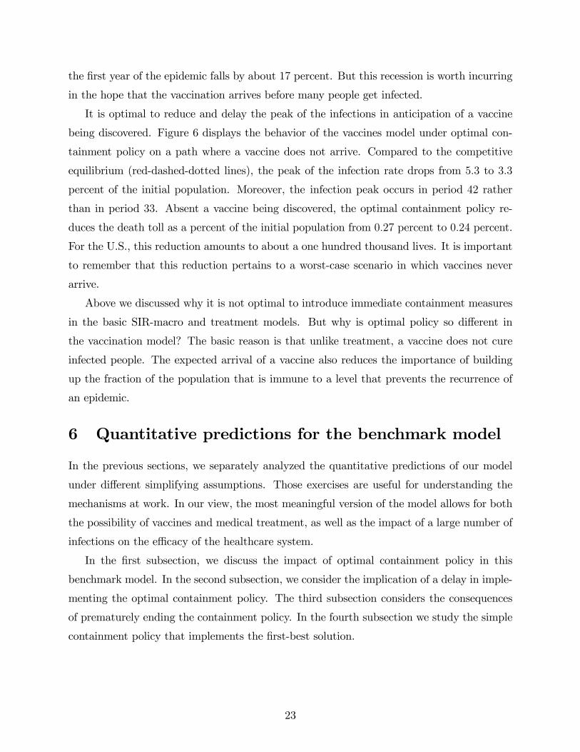
It is optimal to reduce and delay the peak of the infections in anticipation of a vaccine

being discovered. Figure 6 displays the behavior of the vaccines model under optimal con-

tainment policy on a path where a vaccine does not arrive. Compared to the competitive

equilibrium (red-dashed-dotted lines), the peak of the infection rate drops from 5:3 to 3:3

percent of the initial population. Moreover, the infection peak occurs in period 42 rather

than in period 33. Absent a vaccine being discovered, the optimal containment policy re-

duces the death toll as a percent of the initial population from 0:27 percent to 0:24 percent.

For the U.S., this reduction amounts to about a one hundred thousand lives. It is important

to remember that this reduction pertains to a worst-case scenario in which vaccines never

arrive.

Above we discussed why it is not optimal to introduce immediate containment measures

in the basic SIR-macro and treatment models. But why is optimal policy so di§erent in

the vaccination model? The basic reason is that unlike treatment, a vaccine does not cure

infected people. The expected arrival of a vaccine also reduces the importance of building

up the fraction of the population that is immune to a level that prevents the recurrence of

an epidemic.

6 Quantitative predictions for the benchmark model

In the previous sections, we separately analyzed the quantitative predictions of our model

under di§erent simplifying assumptions. Those exercises are useful for understanding the

mechanisms at work. In our view, the most meaningful version of the model allows for both

the possibility of vaccines and medical treatment, as well as the impact of a large number of

infections on the e¢cacy of the healthcare system.

In the Örst subsection, we discuss the impact of optimal containment policy in this

benchmark model. In the second subsection, we consider the implication of a delay in imple-

menting the optimal containment policy. The third subsection considers the consequences

of prematurely ending the containment policy. In the fourth subsection we study the simple

containment policy that implements the Örst-best solution.

23

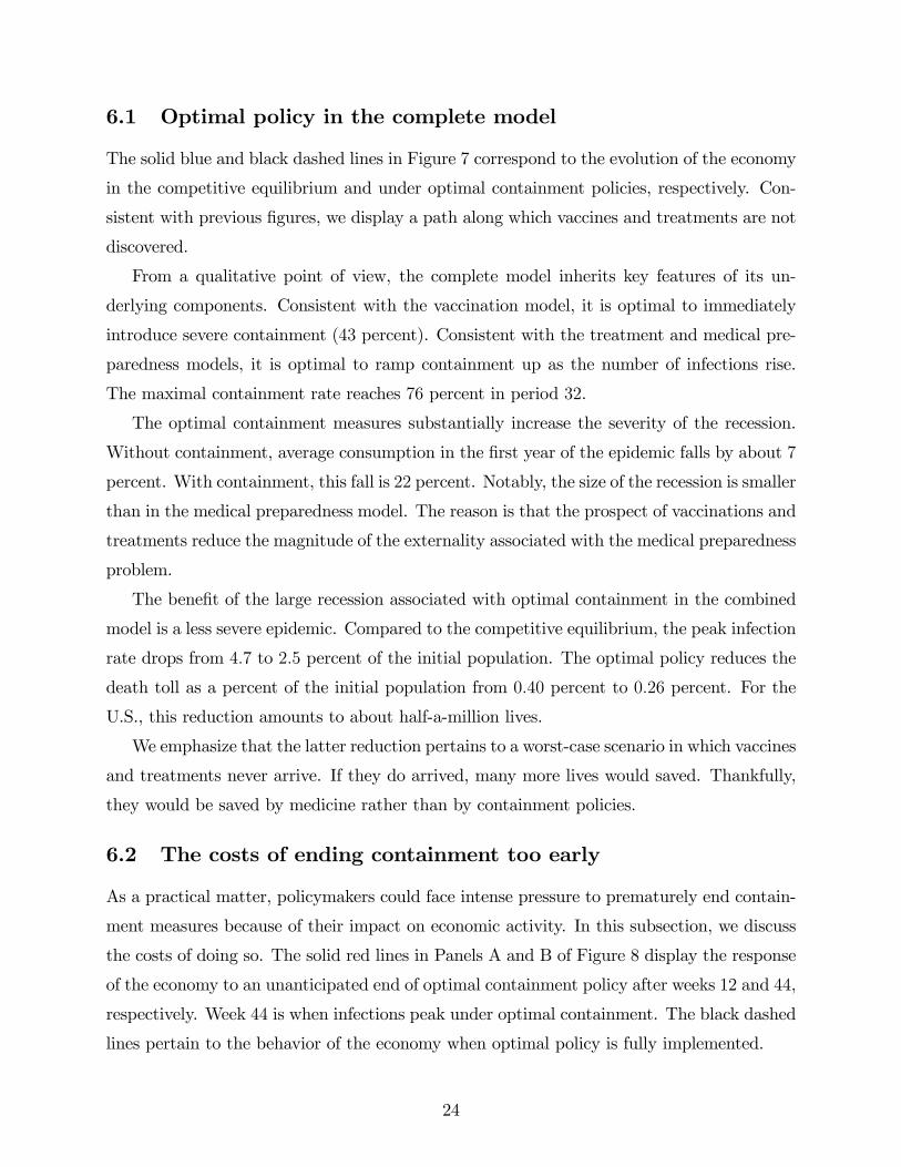
6.1 Optimal policy in the complete model

The solid blue and black dashed lines in Figure 7 correspond to the evolution of the economy

in the competitive equilibrium and under optimal containment policies, respectively. Con-

sistent with previous Ögures, we display a path along which vaccines and treatments are not

discovered.

From a qualitative point of view, the complete model inherits key features of its un-

derlying components. Consistent with the vaccination model, it is optimal to immediately

introduce severe containment (43 percent). Consistent with the treatment and medical pre-

paredness models, it is optimal to ramp containment up as the number of infections rise.

The maximal containment rate reaches 76 percent in period 32.

The optimal containment measures substantially increase the severity of the recession.

Without containment, average consumption in the Örst year of the epidemic falls by about 7

percent. With containment, this fall is 22 percent. Notably, the size of the recession is smaller

than in the medical preparedness model. The reason is that the prospect of vaccinations and

treatments reduce the magnitude of the externality associated with the medical preparedness

problem.

The beneÖt of the large recession associated with optimal containment in the combined

model is a less severe epidemic. Compared to the competitive equilibrium, the peak infection

rate drops from 4:7 to 2:5 percent of the initial population. The optimal policy reduces the

death toll as a percent of the initial population from 0:40 percent to 0:26 percent. For the

U.S., this reduction amounts to about half-a-million lives.

We emphasize that the latter reduction pertains to a worst-case scenario in which vaccines

and treatments never arrive. If they do arrived, many more lives would saved. Thankfully,

they would be saved by medicine rather than by containment policies.

6.2 The costs of ending containment too early

As a practical matter, policymakers could face intense pressure to prematurely end contain-

ment measures because of their impact on economic activity. In this subsection, we discuss

the costs of doing so. The solid red lines in Panels A and B of Figure 8 display the response

of the economy to an unanticipated end of optimal containment policy after weeks 12 and 44,

respectively. Week 44 is when infections peak under optimal containment. The black dashed

lines pertain to the behavior of the economy when optimal policy is fully implemented.

24

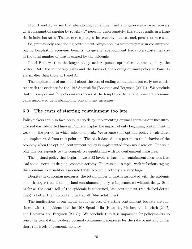
From Panel A, we see that abandoning containment initially generates a large recovery

with consumption surging by roughly 17 percent. Unfortunately, this surge results in a large

rise in infection rates. The latter rise plunges the economy into a second, persistent recession.

So, prematurely abandoning containment brings about a temporary rise in consumption

but no long-lasting economic beneÖts. Tragically, abandonment leads to a substantial rise

in the total number of deaths caused by the epidemic.

Panel B shows that the longer policy makers pursue optimal containment policy, the

better. Both the temporary gains and the losses of abandoning optimal policy in Panel B

are smaller than those in Panel A.

The implications of our model about the cost of ending containment too early are consis-

tent with the evidence for the 1918 Spanish áu (Bootsma and Ferguson (2007)). We conclude

that it is important for policymakers to resist the temptation to pursue transient economic

gains associated with abandoning containment measures.

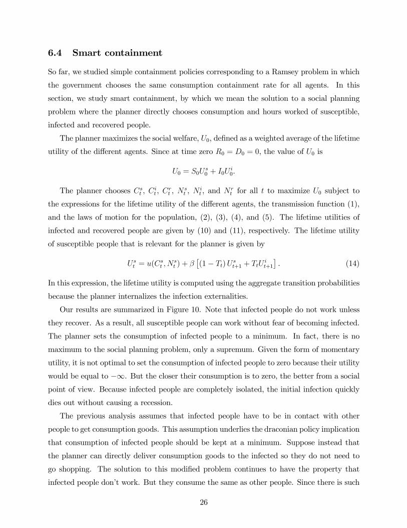
6.3 The costs of starting containment too late

Policymakers can also face pressures to delay implementing optimal containment measures.

The red dashed-dotted lines in Figure 9 display the impact of only beginning containment in

week 33, the period in which infections peak. We assume that optimal policy is calculated

and implemented from that point on. The black dashed lines pertain to the behavior of the

economy when the optimal containment policy is implemented from week zero on. The solid

blue line corresponds to the competitive equilibrium with no containment measures.

The optimal policy that begins in week 33 involves draconian containment measures that

lead to an enormous drop in economic activity. The reason is simple: with infections raging,

the economic externalities associated with economic activity are very large.

Despite the draconian measures, the total number of deaths associated with the epidemic

is much larger than if the optimal containment policy is implemented without delay. Still,

as far as the death toll of the epidemic is concerned, late containment (red dashed-dotted

lines) is better than no containment at all (blue solid lines).

The implications of our model about the cost of starting containment too late are con-

sistent with the evidence for the 1918 Spanish áu (Hatchett, Mecher, and Lipsitch (2007)

and Bootsma and Ferguson (2007)). We conclude that it is important for policymakers to

resist the temptation to delay optimal containment measures for the sake of initially higher

short-run levels of economic activity.

25

6.4 Smart containment

So far, we studied simple containment policies corresponding to a Ramsey problem in which

the government chooses the same consumption containment rate for all agents. In this

section, we study smart containment, by which we mean the solution to a social planning

problem where the planner directly chooses consumption and hours worked of susceptible,

infected and recovered people.

The planner maximizes the social welfare, U0, deÖned as a weighted average of the lifetime

utility of the di§erent agents. Since at time zero R0 = D0 = 0, the value of U0 is

U0 = S0Us0 + I0U

i0.

The planner chooses Cst , Cit , C

rt , N

st , N

it , and N

rt for all t to maximize U0 subject to

the expressions for the lifetime utility of the di§erent agents, the transmission function (1),

and the laws of motion for the population, (2), (3), (4), and (5). The lifetime utilities of

infected and recovered people are given by (10) and (11), respectively. The lifetime utility

of susceptible people that is relevant for the planner is given by

U st = u(Cst ; N

st ) + #

$(1' Tt)U st+1 + TtU

it+1

%. (14)

In this expression, the lifetime utility is computed using the aggregate transition probabilities

because the planner internalizes the infection externalities.

Our results are summarized in Figure 10. Note that infected people do not work unless

they recover. As a result, all susceptible people can work without fear of becoming infected.

The planner sets the consumption of infected people to a minimum. In fact, there is no

maximum to the social planning problem, only a supremum. Given the form of momentary

utility, it is not optimal to set the consumption of infected people to zero because their utility

would be equal to '1. But the closer their consumption is to zero, the better from a social

point of view. Because infected people are completely isolated, the initial infection quickly

dies out without causing a recession.

The previous analysis assumes that infected people have to be in contact with other

people to get consumption goods. This assumption underlies the draconian policy implication

that consumption of infected people should be kept at a minimum. Suppose instead that

the planner can directly deliver consumption goods to the infected so they do not need to

go shopping. The solution to this modiÖed problem continues to have the property that

infected people donít work. But they consume the same as other people. Since there is such

26

a small number of infected people at time zero, aggregate consumption and hours worked

are essentially the same as in the pre-epidemic steady state.

Our simple analysis of smart containment assumes that policy makers know the health

status of di§erent individuals. In reality, this knowledge would require antigen and antibody

tests for immunity and infection that are su¢ciently accurate to act upon. Our results sug-

gest that there are enormous social returns to having these tests and the policy instruments

to implement smart containment.10 This conclusion is consistent with the emphasis placed

by epidemiologist like Ginsberg et al. (2008) on early detection and early response.

7 Related literature

Our work is related to an older literature that combines economics and epidemiology (see

Perrings et. al (2014) for a review). Examples include analyses of how private vaccination

incentives a§ect epidemic dynamics and optimal public-health policy (e.g. Philipson (2000),

Adda (2016) and Manski (2016)).

The COVID-19 crisis has stimulated a quickly growing body of work on the economics

of the epidemic. Below, we brieáy summarize work that is related to our paper.

Atkeson (2020) provides an overview of SIR models and explores their implications for the

COVID-19 epidemic. Alvarez, Argente, and Lippi (2020) study the optimal lock-down policy

in a version of the classic SIR model where the mortality rate increases with the number of

infected people. Toda (2020) uses a SIR model to study the impact of the epidemic on the

stock market.

The paper most closely related to ours is Jones, Philippon, and Venkateswaran (2020).

These authors study analyze optimal mitigation policies in a model where economic activity

and epidemic dynamics interact. Jones et al. (2020) emphasize learning-by-doing in working

from home and assume that people have a fatalism bias about the probability of being

infected in the future. Other di§erences between our paper and theirs are as follows. First,

we explicitly allow for the probabilistic arrival of vaccines and treatments. Second, we

consider we consider the social cost of starting containment too late or ending it too early.

Third, we study ìsmart containmentî policies that make allocations a function of whether

people are infected, susceptible or recovered.

Guerrieri, Lorenzoni, Straub, and Werning (2020) develop a theory of Keynesian supply

10According to de Walque, Friedman and Mattoo (2020), the cost of these tests, including equipment,consumables, protective equipment, and labor, ranges from 2 to 5 dollars.

27

shocks that trigger changes in aggregate demand larger than the shocks themselves. These

authors argue that the economic shocks associated to the COVID-19 epidemic may have this

feature. Guerrieri et al. (2020) analyze the e¢cacy of various Öscal and monetary policies

at dealing with these shocks. In contrast with Guerrieri et al. (2020), we incorporate an

extended version of SIR dynamics into our model.

Berger, Herkenho§, and Mongey (2020) and Stock (2020) study the importance of ran-

domized testing in estimating the health status of the population and designing optimal

mitigation policies. In contrast with these authors, we explicitly model the two-way interac-

tion between infection rates and economic activity.

There is an emerging body of work that studies the e§ects of the COVID-19 epidemic in

models where agents are di§er in their health status as well as other dimensions. In ongoing

work, Glover, Heathcote, Krueger, and Rios-Rull (2020) study optimal mitigation policies in

a model that takes into account the age distribution of the population. Kaplan, Moll, and

Violante (2020) do so in a HANK model.

Faria-e-Castro (2020) studies the e§ect of an epidemic, modeled as a large negative shock

to the utility of consumption of contact-intensive service, in a model with borrowers and

savers. Buera, Fattal-Jaef, Neumeyer, and Shin (2020) study the impact of an unanticipated

lock-down shock in an heterogeneous-agent model.

8 Conclusion

We extend the canonical epidemiology model to study the interaction between economic

decisions and epidemics. In our model, the epidemic generates both supply and demand

e§ects on economic activity. These e§ects work in tandem to generate a large, persistent

recession.

We abstract from many important real-world complications to highlight the basic eco-

nomic forces at work during an epidemic. The central message of our analysis should be

robust to allowing for those complications: there is an inevitable trade-o§ between the

severity of the short-run recession caused by the epidemic and the health consequences of

that epidemic. Dealing with this trade-o§ is a key challenge confronting policymakers.

Our model abstracts from various forces that might a§ect the long-run performance of the

economy. These forces include bankruptcy costs, unemployment hysteresis e§ects, and the

destruction of supply-side chains. It is important to embody these forces in macroeconomic

28

models of epidemics and study their positive and normative implications.

29

References

[1] Adda, JÈrÙme. ìEconomic Activity and the Spread of Viral Diseases: Evidence from

High Frequency Data,î The Quarterly Journal of Economics 131, no. 2 (2016): 891-941.

[2] Alvarez, Fernando, David Argente, Francesco Lippi ìA Simple Planning Problem for

COVID-19 Lockdown,î manuscript, University of Chicago, March 2020.

[3] Atkeson, Andrew ìWhat Will Be The Economic Impact of COVID-19 in the US? Rough

Estimates of Disease Scenarios,î National Bureau of Economic Research, Working Paper

No. 26867, March 2020.

[4] Berger, David Kyle Herkenho§, and Simon Mongey ìAn SEIR Infectious Disease Model

with Testing and Conditional Quarantine,î manuscript, Duke University, March 2020.

[5] Bootsma, Martin CJ, and Neil M. Ferguson. "The E§ect of Public Health Measures

on the 1918 Ináuenza Pandemic in US Cities," Proceedings of the National Academy of

Sciences 104, no. 18 (2007): 7588-7593.

[6] Buera, Francisco, Roberto Fattal-Jaef, Pablo Andres Neumeyer, and Yongseok Shin

ìThe Economic Ripple E§ects of COVID-10,î manuscript, World Bank, 2020.

[7] Damien de Walque, Jed Friedman and Aaditya Mattoo ìTwo Tests for a COVID-19

World,î manuscript, The World Bank, April 2020.

[8] Farhi, Emmanuel and Ivan Werning ìDealing with the Trilemma: Optimal Capital

Controls with Fixed Exchange Rates,î National Bureau of Economic Research Working

Paper No. 18199, June 2012.

[9] Faria-e-Castro, Miguel ìFiscal Policy During a Pandemic,î manuscript, Federal Reserve

Bank of St. Louis, March 2020.

[10] Ferguson, N., Cummings, D., Fraser, C. et al. ìStrategies for Mitigating an Ináuenza

Pandemic,î Nature 442, 448ñ452, 2006.

[11] Ferguson, Neil M., Daniel Laydon, Gemma Nedjati-Gilani, Natsuko Imai, Kylie Ainslie,

Marc Baguelin, Sangeeta Bhatia, Adhiratha Boonyasiri, Zulma Cucunub·, Gina Cuomo-

Dannenburg, Amy Dighe, Ilaria Dorigatti, Han Fu, Katy Gaythorpe, Will Green, Arran

30

Hamlet, Wes Hinsley, Lucy C Okell, Sabine van Elsland, Hayley Thompson, Robert

Verity, Erik Volz, Haowei Wang, Yuanrong Wang, Patrick GTWalker, Caroline Walters,

Peter Winskill, Charles Whittaker, Christl A Donnelly, Steven Riley, and Azra C Ghani,

ìImpact of Non-pharmaceutical Interventions (NPIs) to Reduce COVID- 19 Mortality

and Healthcare Demand,î manuscript, Imperial College, March 2020.

[12] Ginsberg, Jeremy, Matthew H. Mohebbi, Rajan S. Patel, Lynnette Brammer, Mark

S. Smolinski, and Larry Brilliant ìDetecting Ináuenza Epidemics Using Search Engine

Query Data,î manuscript, Centers for Disease Control and Prevention, 2008.

[13] Guerrieri, Veronica, Guido Lorenzoni, Ludwig Straub, and Ivan Werning ìMacroeco-

nomic Implications of COVID-19: Can Negative Supply Shocks Cause Demand Short-

ages?î manuscript, Northwestern University, April 2020.

[14] Gourinchas, Pierre-Olivier. ìFlattening the Pandemic and Recession Curves,î manu-

script, University of California, Berkeley 2020.

[15] Glover, Andrew, Jonathan Heathcote, Dirk Krueger, and JosÈ-Victor RÌos-Rull ìHealth

versus Wealth: On the Distribution E§ects of Controlling a Pandemic,î manuscript,

University of Pennsylvania, 2020.

[16] Hatchett, Richard J., Carter E. Mecher, and Marc Lipsitch. "Public Health Interven-

tions and Epidemic Intensity During the 1918 Ináuenza Pandemic," Proceedings of the

National Academy of Sciences 104, no. 18: 7582-7587, 2007.

[17] Kaplan, Greg, Ben Moll, and Gianluca Violante ìPandemics According to HANK,î

manuscript, University of Chicago, 2020.

[18] Kermack, William Ogilvy, and Anderson G. McKendrick ìA Contribution to the Math-

ematical Theory of Epidemics,î Proceedings of the Royal Society of London, series A

115, no. 772: 700-721, 1927.

[19] Lee, Bruce Y., Shawn T. Brown, Philip C. Cooley, Richard K. Zimmerman, William

D. Wheaton, Shanta M. Zimmer, John J. Grefenstette et al. "A Computer Simulation

of Employee Vaccination to Mitigate an Ináuenza Epidemic," American Journal of

Preventive Medicine 38, no. 3: 247-257, 2010.

31

[20] Moran, Molly ìGuidance on Treatment of the Economic Value of a Statistical Life in

U.S. Department of Transportation Analysesñ2014 Adjustment, U.S. Department of

Transportation, 2016

[21] Perrings, C., Castillo-Chavez, C., Chowell, G., Daszak, P., Fenichel, E.P., Finno§, D.,

Horan, R.D., Kilpatrick, A.M., Kinzig, A.P., Kumino§, N.V. and Levin, S., ìMerging

Economics and Epidemiology to Improve the Prediction and Management of Infectious

Disease,î EcoHealth, 11(4), pp.464-475, 2014.

[22] Philipson, Tomas ìEconomic Epidemiology and Infections Diseases,î in Culyer, A. and

J. Newhouse, Handbook of Health Economics, vol. 1 1761-1799, Elsevier, 2000.

[23] Pueyo, Tomas ìCoronavirus: Why You Must Act Now Politicians, Community Leaders

and Business Leaders: What Should You Do and When?,î Medium, March 10, 2020.

[24] Rajgor, Dimple D. Meng Har Lee, Sophia Archuleta, Natasha Bagdasarian, Swee Chye

Quek ìThe Many Estimates of the COVID-19 Case Fatality Rate,î The Lancet, March

2020.

[25] Riou, Julien and Christian L. Althaus ìPattern of Early Human-to-human Transmission

of Wuhan,î bioR{iv, January 24, 2020.

[26] Stock, James ìCoronavirus Data Gaps and the Policy Response to the Novel Coron-

avirus,î manuscript, Harvard University, 2020.

[27] Toda, Alexis Akira ìSusceptible-Infected-Recovered (SIR) Dynamics of COVID-19 and

Economic Impact,î manuscript, University of California San Diego, 2020.

[28] Viscusi, W.K. and Aldy, J.E. ìThe Value of a Statistical Life: a Critical Review of

Market Estimates Throughout the World,î Journal of Risk and Uncertainty, 27(1),

pp.5-76, 2003.

[29] U.S. Environmental Protection Agency, ìValuing Mortality Risk Reductions for Envi-

ronmental Policy: A White Paper,î 2010.

32

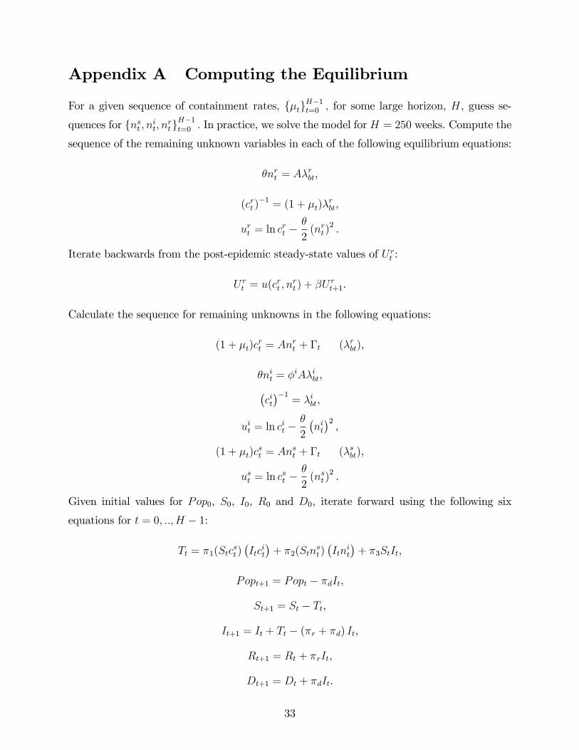
Appendix A Computing the Equilibrium

For a given sequence of containment rates, f)tgH"1t=0 ; for some large horizon, H, guess se-

quences for fnst ; nit; nrtgH"1t=0 : In practice, we solve the model for H = 250 weeks. Compute the

sequence of the remaining unknown variables in each of the following equilibrium equations:

(nrt = A@rbt,

(crt )"1 = (1 + )t)@

rbt,

urt = ln crt '

(

2(nrt )

2 .

Iterate backwards from the post-epidemic steady-state values of U rt :

U rt = u(crt ; n

rt ) + #U

rt+1.

Calculate the sequence for remaining unknowns in the following equations:

(1 + )t)crt = An

rt + 0t (@rbt),

(nit = =iA@ibt,

"cit#"1

= @ibt,

uit = ln cit '

(

2

"nit#2,

(1 + )t)cst = An

st + 0t (@sbt),

ust = ln cst '

(

2(nst)

2 .

Given initial values for Pop0, S0, I0, R0 and D0, iterate forward using the following six

equations for t = 0; ::; H ' 1:

Tt = 41(Stcst)"Itc

it

#+ 42(Stn

st)"Itn

it

#+ 43StIt,

Popt+1 = Popt ' 4dIt,

St+1 = St ' Tt,

It+1 = It + Tt ' (4r + 4d) It,

Rt+1 = Rt + 4rIt,

Dt+1 = Dt + 4dIt.

33

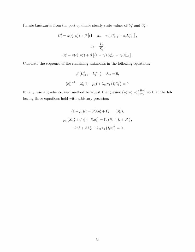
Iterate backwards from the post-epidemic steady-state values of U st and Uit :

U it = u(cit; n

it) + #

$(1' 4r ' 4d)U it+1 + 4rU

rt+1

%,

? t =TtSt,

U st = u(cst ; n

st) + #

$(1' ? t)U st+1 + ? tU

it+1

%.

Calculate the sequence of the remaining unknowns in the following equations:

#"U it+1 ' U

st+1

#' @*t = 0,

(cst)"1 ' @sbt(1 + )t) + @*t41

"ItC

It

#= 0.

Finally, use a gradient-based method to adjust the guesses fnst ; nit; nrtgH"1t=0 so that the fol-

lowing three equations hold with arbitrary precision:

(1 + )t)cit = =

iAnit + 0t (@ibt),

)t"Stc

st + Itc

it +Rtc

rt

#= 0t (St + It +Rt) ,

'(nst + A@sbt + @*t42

"Itn

It

#= 0.

34

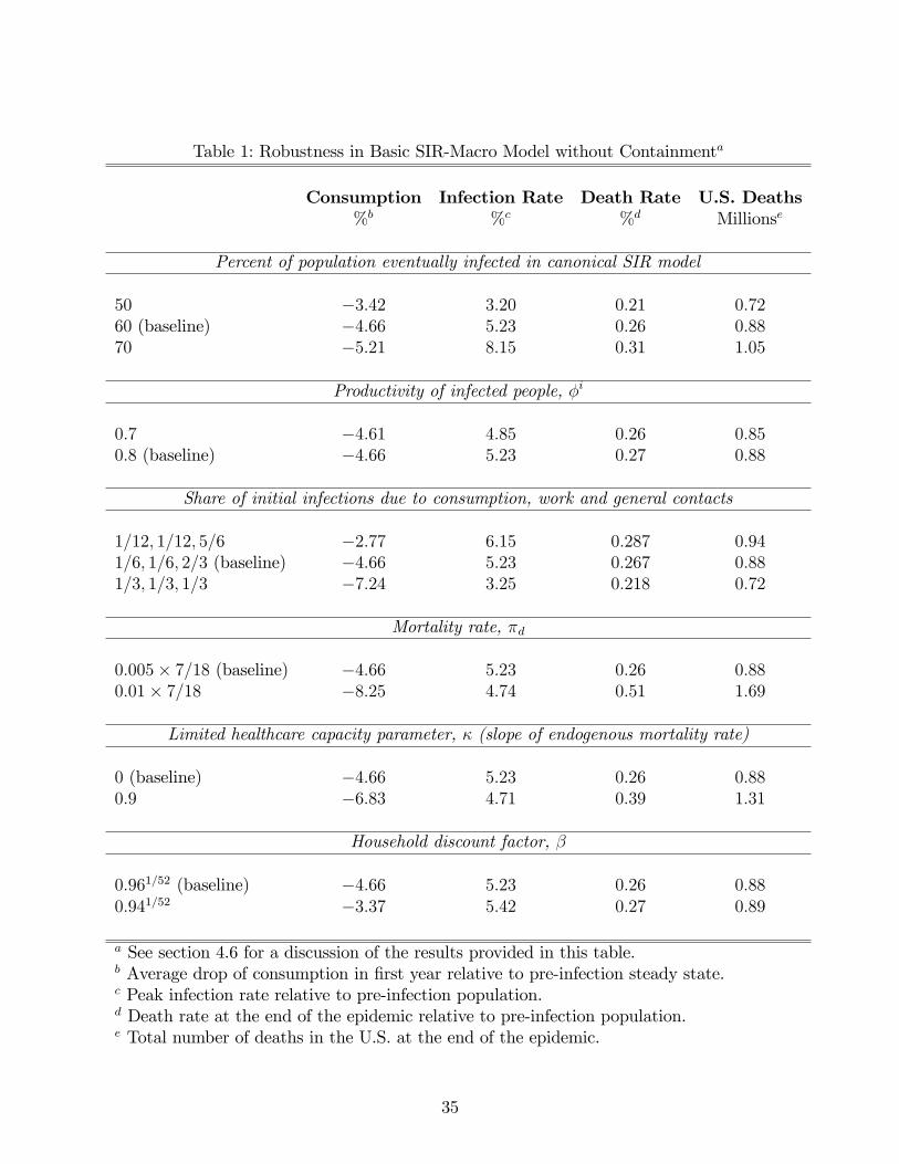
Table 1: Robustness in Basic SIR-Macro Model without Containmenta

Consumption Infection Rate Death Rate U.S. Deaths%b %c %d Millionse

Percent of population eventually infected in canonical SIR model

50 '3:42 3:20 0:21 0:7260 (baseline) '4:66 5:23 0:26 0:8870 '5:21 8:15 0:31 1:05

Productivity of infected people, =i

0:7 '4:61 4:85 0:26 0:850:8 (baseline) '4:66 5:23 0:27 0:88

Share of initial infections due to consumption, work and general contacts

1=12; 1=12; 5=6 '2:77 6:15 0:287 0:941=6; 1=6; 2=3 (baseline) '4:66 5:23 0:267 0:881=3; 1=3; 1=3 '7:24 3:25 0:218 0:72

Mortality rate, 4d

0:005) 7=18 (baseline) '4:66 5:23 0:26 0:880:01) 7=18 '8:25 4:74 0:51 1:69

Limited healthcare capacity parameter, A (slope of endogenous mortality rate)

0 (baseline) '4:66 5:23 0:26 0:880:9 '6:83 4:71 0:39 1:31

Household discount factor, #

0:961=52 (baseline) '4:66 5:23 0:26 0:880:941=52 '3:37 5:42 0:27 0:89

a See section 4.6 for a discussion of the results provided in this table.b Average drop of consumption in Örst year relative to pre-infection steady state.c Peak infection rate relative to pre-infection population.d Death rate at the end of the epidemic relative to pre-infection population.e Total number of deaths in the U.S. at the end of the epidemic.

35

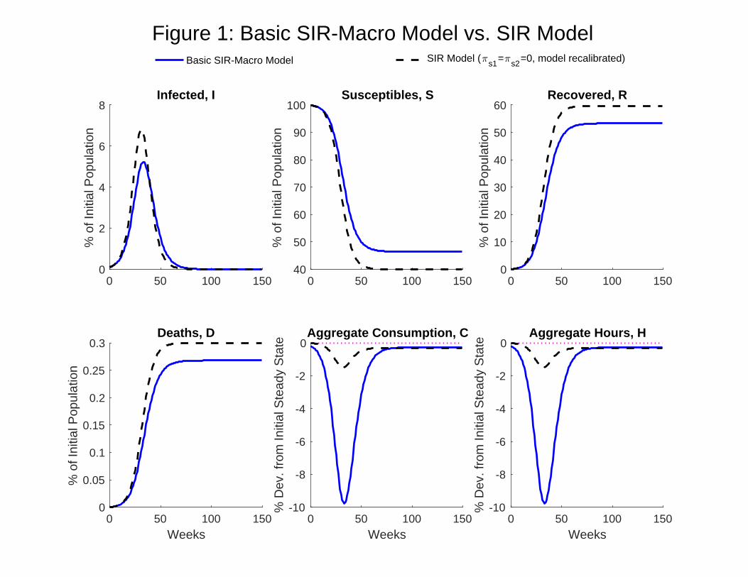
0 50 100 15040

50

60

70

80

90

100

% o

f Ini

tial P

opul

atio

n

Susceptibles, S

0 50 100 1500

10

20

30

40

50

60

% o

f Ini

tial P

opul

atio

n

Recovered, R

0 50 100 150Weeks

0

0.05

0.1

0.15

0.2

0.25

0.3

% o

f Ini

tial P

opul

atio

n

Deaths, D

0 50 100 150Weeks

-10

-8

-6

-4

-2

0

% D

ev. f

rom

Initi

al S

tead

y St

ate Aggregate Consumption, C

0 50 100 150Weeks

-10

-8

-6

-4

-2

0

% D

ev. f

rom

Initi

al S

tead

y St

ate Aggregate Hours, H

Figure 1: Basic SIR-Macro Model vs. SIR Model

0 50 100 1500

2

4

6

8%

of I

nitia

l Pop

ulat

ion

Infected, I

Basic SIR-Macro Model SIR Model ( s1= s2=0, model recalibrated)

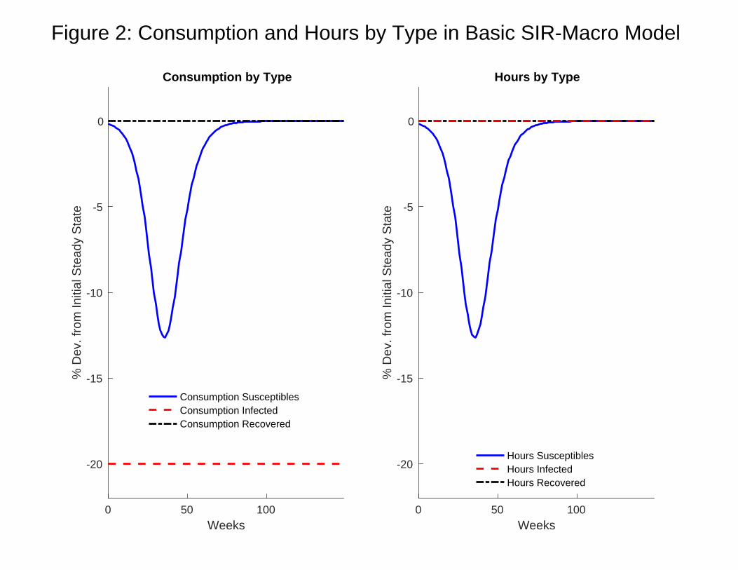
0 50 100Weeks

-20

-15

-10

-5

0

% D

ev. f

rom

Initi

al S

tead

y St

ate

Consumption by Type

Consumption SusceptiblesConsumption InfectedConsumption Recovered

Figure 2: Consumption and Hours by Type in Basic SIR-Macro Model

0 50 100Weeks

-20

-15

-10

-5

0

% D

ev. f

rom

Initi

al S

tead

y St

ate

Hours by Type

Hours SusceptiblesHours InfectedHours Recovered

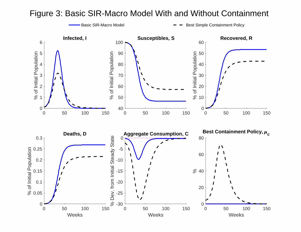
0 50 100 15040

50

60

70

80

90

100

% o

f Ini

tial P

opul

atio

n

Susceptibles, S

0 50 100 1500

10

20

30

40

50

60

% o

f Ini

tial P

opul

atio

n

Recovered, R

0 50 100 150Weeks

0

0.05

0.1

0.15

0.2

0.25

0.3

% o

f Ini

tial P

opul

atio

n

Deaths, D

0 50 100 150Weeks

-30

-25

-20

-15

-10

-5

0

% D

ev. f

rom

Initi

al S

tead

y St

ate Aggregate Consumption, C

0 50 100 150Weeks

0

20

40

60

80

%

Best Containment Policy, c

Figure 3: Basic SIR-Macro Model With and Without Containment

0 50 100 1500

1

2

3

4

5

6%

of I

nitia

l Pop

ulat

ion

Infected, I

Basic SIR-Macro Model Best Simple Containment Policy

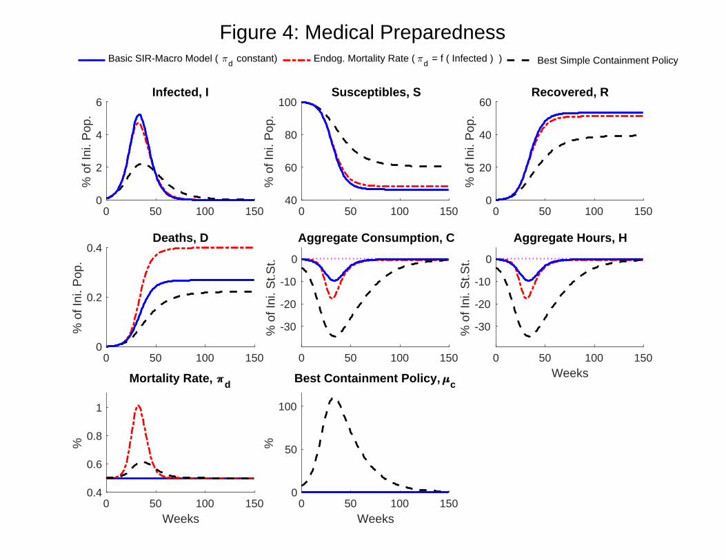
0 50 100 15040

60

80

100

% o

f Ini

. Pop

.

Susceptibles, S

0 50 100 1500

20

40

60

% o

f Ini

. Pop

.

Recovered, R

0 50 100 1500

0.2

0.4

% o

f Ini

. Pop

.

Deaths, D

0 50 100 150

-30

-20

-10

0%

of I

ni. S

t.St.

Aggregate Consumption, C

0 50 100 150Weeks

-30

-20

-10

0

% o

f Ini

. St.S

t.

Aggregate Hours, H

0 50 100 150Weeks

0.4

0.6

0.8

1

%

Mortality Rate, d

0 50 100 150Weeks

0

50

100

%

Best Containment Policy, c

Figure 4: Medical Preparedness

0 50 100 1500

2

4

6%

of I

ni. P

op.

Infected, I

Basic SIR-Macro Model ( d constant) Endog. Mortality Rate ( d = f ( Infected ) ) Best Simple Containment Policy

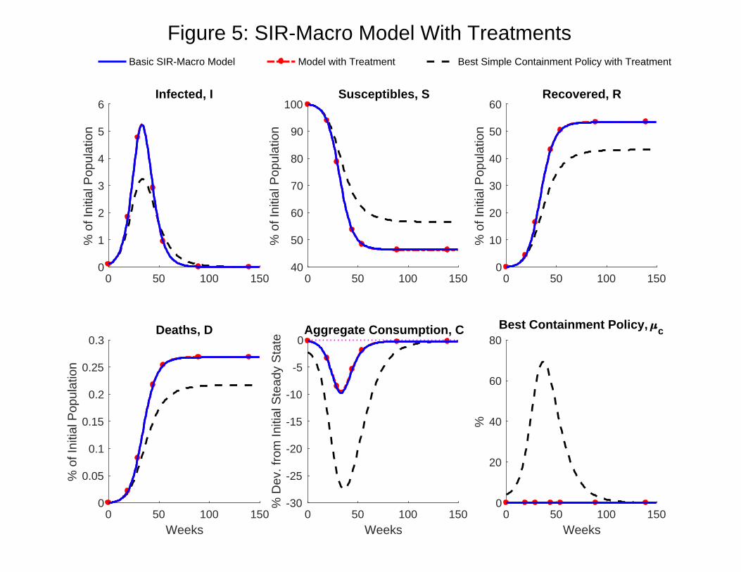
0 50 100 15040

50

60

70

80

90

100

% o

f Ini

tial P

opul

atio

n

Susceptibles, S

0 50 100 1500

10

20

30

40

50

60

% o

f Ini

tial P

opul

atio

n

Recovered, R

0 50 100 150Weeks

0

0.05

0.1

0.15

0.2

0.25

0.3

% o

f Ini

tial P

opul

atio

n

Deaths, D

0 50 100 150Weeks

-30

-25

-20

-15

-10

-5

0

% D

ev. f

rom

Initi

al S

tead

y St

ate Aggregate Consumption, C

0 50 100 150Weeks

0

20

40

60

80

%

Best Containment Policy, c

Figure 5: SIR-Macro Model With Treatments

0 50 100 1500

1

2

3

4

5

6%

of I

nitia

l Pop

ulat

ion

Infected, I

Basic SIR-Macro Model Model with Treatment Best Simple Containment Policy with Treatment

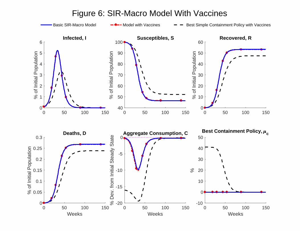
0 50 100 15040

50

60

70

80

90

100

% o

f Ini

tial P

opul

atio

n

Susceptibles, S

0 50 100 1500

10

20

30

40

50

60

% o

f Ini

tial P

opul

atio

n

Recovered, R

0 50 100 150Weeks

0

0.05

0.1

0.15

0.2

0.25

0.3

% o

f Ini

tial P

opul

atio

n

Deaths, D

0 50 100 150Weeks

-20

-15

-10

-5

0

% D

ev. f

rom

Initi

al S

tead

y St

ate Aggregate Consumption, C

0 50 100 150Weeks

-10

0

10

20

30

40

50

%

Best Containment Policy, c

Figure 6: SIR-Macro Model With Vaccines

0 50 100 1500

1

2

3

4

5

6%

of I

nitia

l Pop

ulat

ion

Infected, I

Basic SIR-Macro Model Model with Vaccines Best Simple Containment Policy with Vaccines

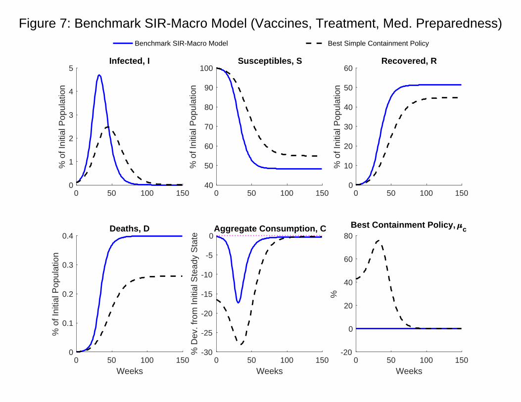
0 50 100 15040

50

60

70

80

90

100

% o

f Ini

tial P

opul

atio

n

Susceptibles, S

0 50 100 1500

10

20

30

40

50

60

% o

f Ini

tial P

opul

atio

n

Recovered, R

0 50 100 150Weeks

0

0.1

0.2

0.3

0.4

% o

f Ini

tial P

opul

atio

n

Deaths, D

0 50 100 150Weeks

-30

-25

-20

-15

-10

-5

0

% D

ev. f

rom

Initi

al S

tead

y St

ate Aggregate Consumption, C

0 50 100 150Weeks

-20

0

20

40

60

80

%

Best Containment Policy, c

Figure 7: Benchmark SIR-Macro Model (Vaccines, Treatment, Med. Preparedness)

0 50 100 1500

1

2

3

4

5%

of I

nitia

l Pop

ulat

ion

Infected, I

Benchmark SIR-Macro Model Best Simple Containment Policy

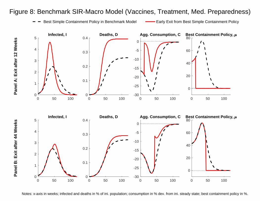
0 50 1000

0.1

0.2

0.3

0.4Deaths, D

0 50 100-30

-25

-20

-15

-10

-5

0

Agg. Consumption, C

0 50 100

0

20

40

60

80Best Containment Policy,

0 50 1000

1

2

3

4

5Infected, I

Pane

l A: E

xit a

fter 1

2 W

eeks

0 50 1000

0.1

0.2

0.3

0.4Deaths, D

0 50 100-30

-25

-20

-15

-10

-5

0

Agg. Consumption, C

0 50 100

0

20

40

60

80Best Containment Policy,

Figure 8: Benchmark SIR-Macro Model (Vaccines, Treatment, Med. Preparedness)

0 50 1000

1

2

3

4

5Infected, I

Pane

l B: E

xit a

fter 4

4 W

eeks

Notes: x-axis in weeks; infected and deaths in % of ini. population; consumption in % dev. from ini. steady state; best containment policy in %.

Best Simple Containment Policy in Benchmark Model Early Exit from Best Simple Containment Policy

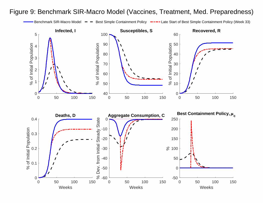
0 50 100 15040

50

60

70

80

90

100

% o

f Ini

tial P

opul

atio

n

Susceptibles, S

0 50 100 1500

10

20

30

40

50

60

% o

f Ini

tial P

opul

atio

n

Recovered, R

0 50 100 150Weeks

0

0.1

0.2

0.3

0.4

% o

f Ini

tial P

opul

atio

n

Deaths, D

0 50 100 150Weeks

-60

-50

-40

-30

-20

-10

0

% D

ev. f

rom

Initi

al S

tead

y St

ate Aggregate Consumption, C

0 50 100 150Weeks

-50

0

50

100

150

200

250

%

Best Containment Policy, c

Figure 9: Benchmark SIR-Macro Model (Vaccines, Treatment, Med. Preparedness)

0 50 100 1500

1

2

3

4

5%

of I

nitia

l Pop

ulat

ion

Infected, I

Benchmark SIR-Macro Model Best Simple Containment Policy Late Start of Best Simple Containment Policy (Week 33)

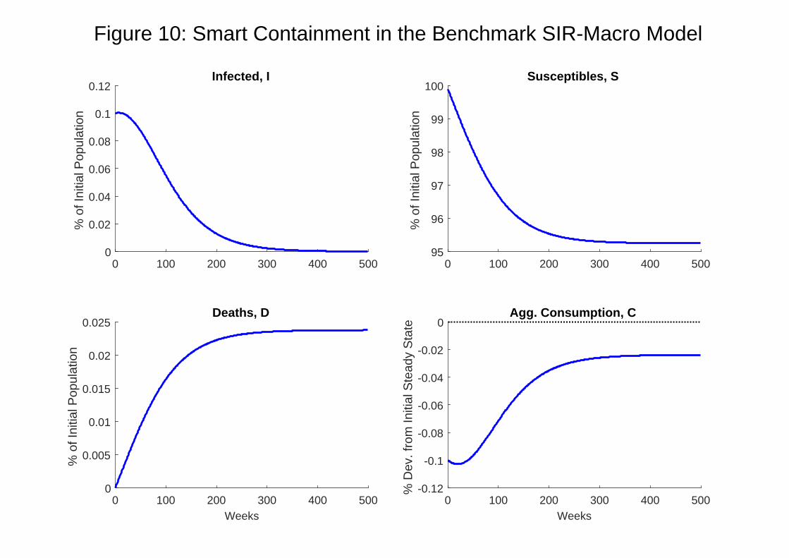
0 100 200 300 400 5000

0.02

0.04

0.06

0.08

0.1

0.12%

of I

nitia

l Pop

ulat

ion

Infected, I

0 100 200 300 400 50095

96

97

98

99

100

% o

f Ini

tial P

opul

atio

n

Susceptibles, S

0 100 200 300 400 500Weeks

0

0.005

0.01

0.015

0.02

0.025

% o

f Ini

tial P

opul

atio

n

Deaths, D

Figure 10: Smart Containment in the Benchmark SIR-Macro Model

0 100 200 300 400 500Weeks

-0.12

-0.1

-0.08

-0.06

-0.04

-0.02

0

% D

ev. f

rom

Initi

al S

tead

y St

ate

Agg. Consumption, C