The Low Beta Anomaly: A Decomposition into Micro and Macro Effects

Malcolm Baker*

Brendan Bradley

Ryan Taliaferro

September 13, 2013

Abstract

Low beta stocks have offered a combination of low risk and high returns. We decompose the

anomaly into micro and macro components. The micro component comes from the selection of

low beta stocks. The macro component comes from the selection of low beta countries or

industries. The two parts both contribute to the low beta anomaly, with important implications

for the construction of managed volatility portfolios.

* Malcolm Baker is professor of finance at Harvard Business School, research associate at the National Bureau of

Economic Research, and senior consultant at Acadian Asset Management, Boston. Brendan Bradley is director of

portfolio management at Acadian Asset Management, Boston. Ryan Taliaferro is portfolio manager at Acadian

Asset Management, Boston.

Note: The views expressed herein are those of the authors and do not necessarily reflect the views of the National

Bureau of Economic Research or Acadian Asset Management.

1

In an efficient market, investors earn a higher return only to the extent that they bear higher risk.

Despite the intuitive appeal of a positive risk-return relationship, this pattern has been

surprisingly hard to find in the data, dating at least to Black (1972). For example, sorting stocks

using measures of market beta or volatility shows just the opposite. Panel A of Figure 1 shows

that, from 1968 through 2012 in the U.S. equity market, portfolios of low risk stocks deliver on

the promise of lower risk as planned, but with surprisingly higher average returns. A dollar

invested in the lowest risk portfolio grew to $81.66 while a dollar invested in the highest risk

portfolio grew to only $9.76. A similar inverse relationship between risk and return appears from

1989 through 2012 in a sample of up to 31 developed equity markets shown in Panel B of Figure

1. A dollar invested in the lowest risk portfolio of global equities grew to $7.23. Meanwhile a

dollar invested in the highest risk portfolio of global equities grew to only $1.20 at the end of the

period. This so-called low risk anomaly suggests a very basic form of market inefficiency.

Shiller (2001) credits Paul Samuelson with the idea of separating market efficiency into

two types. Micro efficiency concerns the relative pricing of individual stocks, while macro

efficiency refers to the pricing of the market as a whole. Broadly speaking, inefficiencies can be

examined at different levels of aggregation: at the individual stock level, at the industry level, at

the country level, or, in some cases, for global equity markets.

Samuelson (1998) conjectured that capital markets have “come a long way, baby, in two

hundred years toward micro efficiency of markets: Black-Scholes option pricing, indexing of

portfolio diversification, and so forth. But there is no persuasive evidence, either from economic

history or avant garde theorizing, that macro market inefficiency is trending toward extinction.”

At the heart of the difference is the fact that individual securities often have close substitutes. As

Scholes (1972) shows, the availability of close substitutes facilitates low risk micro arbitrage and

2

pins down relative prices, if there are no practical limits on arbitrage. Industry and country

portfolios have fewer close substitutes, and the equity market as a whole has none. So, individual

stocks, in this view, are priced more efficiently relative to each other than they are in absolute

terms. Of course, limits to arbitrage are real and substitutes are never perfect, so even

Samuelson’s hypothesis is one of relative not absolute efficiency.

In the context of the low risk anomaly, Baker, Bradley, and Wurgler (2011) emphasize

the important constraint that long only, fixed-benchmark mandates impose on micro arbitrage.

Many institutional investors are judged not by total return relative to total risk, but instead on

active return relative to active risk, or benchmark tracking error. Such benchmark oriented

mandates discourage investment in low risk stocks. Despite their low risk, these stocks only

become attractive relative to the tracking error they create when their anticipated return exceeds

the benchmark in absolute terms. There are also limits on macro arbitrage. Market aggregates do

not have close substitutes, and so macro arbitrage – in the usual sense of simultaneously buying

low and selling fundamentally similar securities high – is largely infeasible. Standard

institutional mandates and risk management practices also play a role here, typically limiting the

size of benchmark relative country or industry exposures or eliminating them entirely through

narrow mandates that identify a single country index as the benchmark return. French and

Poterba (1991) and more recently Ahearne, Griever, and Warnock (2004) document a home bias,

for example, showing that individuals often do not invest across borders.

One way of examining the relative efficiency of markets at different levels of aggregation

is to aggregate or disaggregate a known anomaly into its micro and macro components. An

important limitation of this approach is that anomalies change their meaning at different levels of

aggregation. Ratios of fundamental to market value capture misvaluation at the individual stock

3

level, as in Basu (1977). But, Lewellen (1999) finds little contribution from the industry level,

where differences in valuation ratios might reflect varying approaches to caplitalizing investment

or reporting earnings. Meanwhile, Fama and French (1998) find that predictive power reappears

at even higher levels of aggregation in cross-country regressions. Likewise, Kothari and Shanken

(1997) find that time series comparisons of valuation ratios for equity markets as a whole are

also useful. Unlike value, beta retains the same meaning at the stock level and in country and

industry portfolios, though it loses some of its variability. Its usefulness runs out for the market

as a whole, where it is 1.0 by definition. Another limitation of aggregation is that econometric

tests typically lose power to identify inefficiency. So, it is important to consider economic and

statistical significance.

In the spirit of Samuelson, we decompose the low risk anomaly into its micro and macro

components. The pattern of low risk and high return can in principle come either from the macro

selection of lower risk countries and industries or from the micro selection of low risk stocks

within those countries and industries. We separate the two effects by forming long-short

portfolios of stocks that first hold constant ex ante country or industry level risk and examine

stock selection. Then, we hold constant ex ante stock level risk and examine country or industry

selection. What we find in a sample of 29 US industries and up to 31 developed countries is that

micro and macro selection both contribute to the low risk anomaly, albeit for two surprisingly

different reasons.

The micro selection of stocks leads to a significant reduction in risk, with only a modest

difference in return. Even holding constant country or industry level risk, there is ample

opportunity to form lower risk portfolios through stock selection, and these lower risk portfolios

do not suffer lower returns. High risk stocks can be distinctly identified within the utility industry

4

or in Japan, for example, but they have similar raw returns on average when compared to low

risk stocks in the same industry or country grouping. This evidence supports the notion of limits

to micro arbitrage in low risk stocks that come from traditional fixed-benchmark mandates.

Meanwhile, the macro selection of countries in particular leads to increases in return, with only

modest differences in risk. Countries that we identify as high risk ex ante are only modestly

higher risk going forward, but they have distinctly lower returns. This evidence supports the

limits to macro arbitrage across countries and industries.

Other researchers have examined the question of micro versus macro efficiency. Jung and

Shiller (2005) show that dividend yields predict the growth in dividends at the firm level, but not

at higher levels of aggregation. A higher dividend yield should intuitively be associated with

lower growth in dividends, and indeed across firms this is true, suggesting a degree of micro

efficiency. Somewhat pathologically, higher aggregate dividend yields predict higher, not lower,

dividend growth, suggesting macro inefficiency. This parallels the more in-depth studies by

Campbell (1991) and Vuolteenaho (2002) of variance decompositions of stock returns using

valuation ratios. Lamont and Stein (2006) extend this logic to corporate finance. Corporate

financing activities like new issuance and stock-financed mergers, which are in part designed to

take advantage of market inefficiency, display greater sensitivity to aggregate movements in

value than they do to individual stock price changes.

Decomposing the low risk anomaly is a particularly appealing new avenue, because beta

retains its meaning in country and industry aggregations. Unlike beta, value or momentum, for

example have no ex ante, risk-based theory of return predictability. So, if value, to take an

example, has greater predictive power within industries than across industries, little is revealed

about micro versus macro efficiency. It may simply be differences in accounting conventions, for

5

example, across industries, which make relative value comparisons with financial statement data

easier within industries.

Our results on the decomposition of the low risk anomaly into micro and macro effects

have investment implications for plan sponsors and individuals alike. For individuals, it suggests

that trying to exploit the mispricing through industry and sector funds or ETFs will only get you

so far. While such a strategy can gain exposure to the macro effects, it cannot exploit

considerable risk reduction available in micro stock selection. For institutional investors and plan

sponsors, it suggests that perfunctory approaches to risk modeling and overly constrained

mandates will not fully appreciate the benefits of the macro effects. Broad mandates with loose

constraints and thoughtful techniques to modeling risk will do the most to exploit the low risk

anomaly.

The Low Risk Anomaly

A preliminary step is confirming that the low risk anomaly is present in two sources of stock

return data that are convenient for our decomposition. We sort stocks into quintiles according to

ex ante market beta and form five capitalization-weighted, buy-and-hold portfolios. Theory

predicts a positive relationship between risk and return. Under the Sharpe-Lintner Capital Asset

Pricing Model, the relationship is linear and the slope between contemporaneously measured

market beta and returns is equal to the overall market risk premium. Fortunately, the low risk

anomaly does not hinge on elaborate estimations, because the empirical slope has the wrong

sign.

6

For our analysis of industries within the U.S., we use data from the Center for Research

in Securities Prices (CRSP). From CRSP we collect the monthly returns of all U.S. shares for the

period January 1963 through December 2012. We also collect the corresponding data on market

capitalizations to form capitalization-weighted portfolios. Each month and for each stock, we

estimate a market beta using the previous 60 months of excess returns. Stocks that have fewer

than 60 prior monthly returns are included if they have a history of at least 12 months.

For our analysis of countries across the developed world, we use data from Standard &

Poor’s Broad Market Index (BMI). From BMI we collect monthly and weekly returns and

market capitalizations for common stocks for the period July 1989 through December 2012. The

raw dataset contains a very small number of suspicious returns, less than –100% and greater than

1,000%, and we exclude these observations from our analysis. Market betas are estimated using

the excess return of the capitalization-weighted aggregate of all stocks in the sample as the

market portfolio. Returns are measured in U.S. dollars, and the risk-free rate is the U.S. Treasury

bill rate from Ken French’s website. Each month and for each stock, we estimate a market beta

using the previous 60 weeks of returns. Stocks that have fewer than 60 prior weekly returns are

included if they have a history of at least 12 weeks. We opt for a more dynamic estimation of

betas in the BMI. The overall sample is shorter and a five-year period to estimate initial betas is

more costly. Neither monthly nor weekly country betas perform particularly well in predicting

future country portfolio betas, but weekly measures are a marginal improvement.

Figure 1 depicts the low risk anomaly graphically. In the CRSP data in Panel A, a $1

investment in the low risk quintile portfolio in 1968 compounds to $81.66 by the end of 2012. A

$1 investment in the high risk quintile compounds to only $9.76. Over the shorter history of the

7

BMI data, a $1 investment in 1989 compounded to $7.23 in the low risk quintile and $1.20 in the

high risk quintile.

To understand the statistical significance of these results, we perform a simple test in

Table 1. We regress the returns of each of the resulting five portfolios, measured in excess of

U.S. Treasury bill returns, on the aggregate market excess return, to find the portfolio’s full-

period ex post market beta and CAPM alpha. The first and third columns in Table 1 report the

betas and alphas, respectively, of five CRSP portfolios. The second and fourth columns in Table

1 report the same calculations for the BMI data. For example, the portfolio formed from the

CRSP stocks with the lowest betas realized a beta of 0.59 over the full period, 1968-2012. The

portfolio formed from the CRSP stocks with the highest betas realized a beta of 1.61. The

difference between these betas of 1.02 is both large and significant, with a t-statistic of 23.99.

These results suggest that betas estimated from past returns are strong predictors of future betas.

More importantly, the third column in Table 1 reports the alphas for five CRSP, beta-

sorted portfolios. The difference in risk-adjusted performance is stark. The least risky portfolio

formed from the lowest beta stocks has an alpha of 2.27% and a t-statistic 2.16, while the riskiest

portfolio formed from the highest beta stocks has a CAPM alpha of –4.49% and t-statistic of

–2.70. The difference between these alphas is economically large at 6.76% and statistically

significant with a t-statistic of 2.84. It is this last result that summarizes the low-risk anomaly:

low risk stocks outperform high risk stocks on a risk-adjusted basis.

Despite a shorter history, the low risk anomaly appears to be stronger in the BMI data.

The fourth column in Table 1 reports the alphas for five BMI, beta-sorted portfolios. The

difference between the alphas is larger at 9.24%, with a t-statistic of 2.71. This is not quite an

8

independent test of the low risk anomaly, because the samples overlap in time and in securities

with the U.S. included in both. However, when we exclude the two largest countries, the U.S.

and Japan, we obtain similar results both here and in the decomposition below. Our aim is to use

data, with the highest quality and deepest history, for separate industry and country

decompositions. We sacrifice cross country variation to double the history of our industry

decomposition, and we sacrifice history to have a stable cross-country decomposition.

These preliminary results align with the literature, which dates to Black (1972), Black,

Jensen, and Scholes (1972), Haugen and Heins (1975). More recently, Fama and French (1992),

Falkenstein (1994) and others have observed a flat or even negative empirical relationship

between risk and return. Ang, Hodrick, Xing, and Zhang (2006, 2009) focused more on volatility

sorts, pointing out the poor performance of the highest volatility quantiles. Bali, Cakici, and

Whitelaw (2011) develop a related measure of lottery-like risk. Hong and Sraer (2012)

incorporate speculative motives to trade into an asset pricing model to explain the low risk

anomaly while Frazzini and Pederson (2010) focus on the implications of leverage and

margining and extend this to other asset classes. There is roughly a risk return tradeoff across

long histories of asset class returns, where stocks outperform bonds, for example. But, within

asset classes, the lowest risk portfolios have higher Sharpe ratios. Baker and Haugen (2012) and

Blitz, Pang and van Vliet (2012) document the outperformance of low risk stocks in various

markets throughout the developed and emerging world. None of these authors focus on the

decomposition of the anomaly into micro and macro effects. In a current working paper, Asness,

Frazzini, and Pedersen (2013) apply a different methodology to examine the contributions to the

low risk anomaly of the industry and stock selection pieces. Their results are consistent with our

own decomposition at the industry level.

9

Explanations have emphasized a combination of behavioral demand and the limits to

arbitrage, including limited borrowing capacity and the delegation of stock selection, to explain

the low risk anomaly. Baker, Bradley, and Wurgler (2011) survey three behavioral explanations:

lottery preferences, representativeness, and overconfidence. We omit a detailed review of these

here to save space. In terms of constraints, Black (1972) and Frazzini and Pedersen (2010)

emphasize leverage. Karceski (2002) and Baker, Bradley, and Wurgler (2011) focus on the

effects of intermediation. While Karceski describes the interaction between high beta strategies

and the capture of mutual fund flows, Baker, Bradley, and Wurgler derive the implications of

fixed benchmark strategies for low risk stocks using the framework in Brennan (1993). It is

worth noting that these stories suggest both the overvaluation of high risk stocks and the

undervaluation of low risk stocks. Our focus here is not to disentangle the absolute mispricing,

but rather to examine the relative mispricing in Table 1. Assuming the behavioral demand

applies to both individual stocks and market aggregates, a decomposition of the low risk

anomaly can in principle help to understand the extent of the limits to micro and macro arbitrage,

and the role of fixed benchmarks.

Variations on the Low Risk Anomaly

There are several important footnotes to this analysis so far. The first involves the rate of

turnover and liquidity in the low risk portfolios. The second involves the benchmark model used

for computing risk-adjusted returns, or alphas. The third is the measure of risk itself, which has

varied in the literature.

10

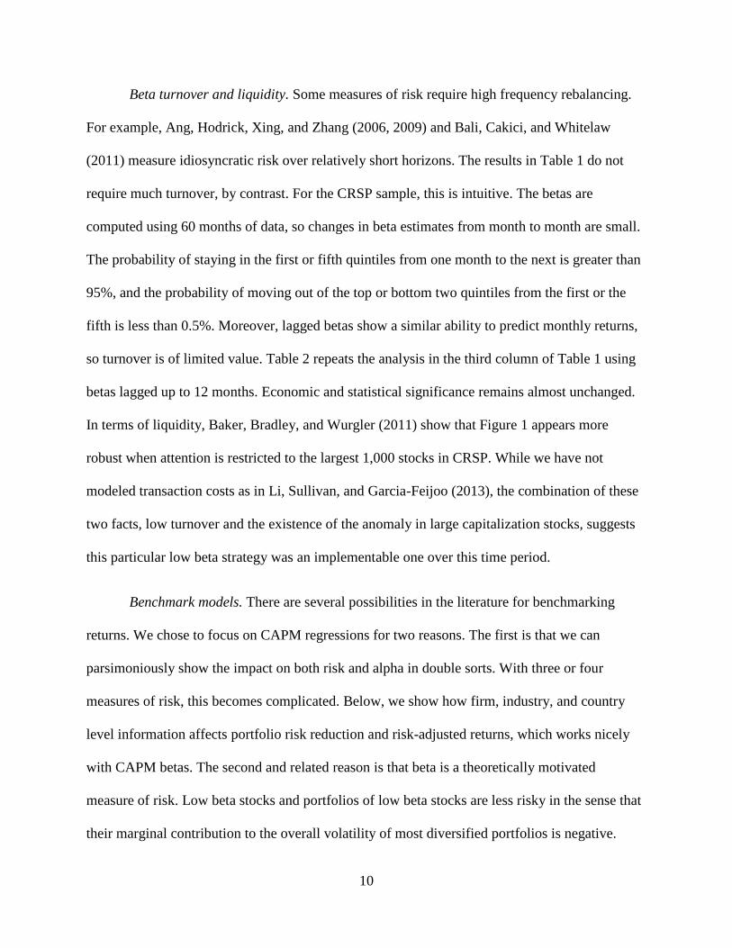
Beta turnover and liquidity. Some measures of risk require high frequency rebalancing.

For example, Ang, Hodrick, Xing, and Zhang (2006, 2009) and Bali, Cakici, and Whitelaw

(2011) measure idiosyncratic risk over relatively short horizons. The results in Table 1 do not

require much turnover, by contrast. For the CRSP sample, this is intuitive. The betas are

computed using 60 months of data, so changes in beta estimates from month to month are small.

The probability of staying in the first or fifth quintiles from one month to the next is greater than

95%, and the probability of moving out of the top or bottom two quintiles from the first or the

fifth is less than 0.5%. Moreover, lagged betas show a similar ability to predict monthly returns,

so turnover is of limited value. Table 2 repeats the analysis in the third column of Table 1 using

betas lagged up to 12 months. Economic and statistical significance remains almost unchanged.

In terms of liquidity, Baker, Bradley, and Wurgler (2011) show that Figure 1 appears more

robust when attention is restricted to the largest 1,000 stocks in CRSP. While we have not

modeled transaction costs as in Li, Sullivan, and Garcia-Feijoo (2013), the combination of these

two facts, low turnover and the existence of the anomaly in large capitalization stocks, suggests

this particular low beta strategy was an implementable one over this time period.

Benchmark models. There are several possibilities in the literature for benchmarking

returns. We chose to focus on CAPM regressions for two reasons. The first is that we can

parsimoniously show the impact on both risk and alpha in double sorts. With three or four

measures of risk, this becomes complicated. Below, we show how firm, industry, and country

level information affects portfolio risk reduction and risk-adjusted returns, which works nicely

with CAPM betas. The second and related reason is that beta is a theoretically motivated

measure of risk. Low beta stocks and portfolios of low beta stocks are less risky in the sense that

their marginal contribution to the overall volatility of most diversified portfolios is negative.

11

Size, value, and momentum are other anomalies that were discovered because of their return

properties not because of any clear risk-based theory.

Even if size and value can also be considered anomalous, it is still useful to ask whether

beta sorts represent a different anomaly from value and size. As it turns out, low risk alphas are

still statistically significant with controls for value and size. The alpha in Table 1 retains its

statistical significance, but the point estimate drops from 6.76 to 4.08. What this says is that there

is incremental information in beta that is not fully contained in value, and also that some of the

alpha in low risk strategies can be captured through value. This is not too surprising, in that any

explanation where low risk stocks are undervalued predicts that crude value measures absorb

some of the low risk anomaly. Like value, momentum helps to explain some of the performance

of low beta strategies. Momentum alone does not eliminate the low beta outperformance, but it

also reduces its economic and statistical power somewhat. However, there is even less reason to

include momentum in the benchmark. While the correlation between value or size and beta is

stable, the connection between momentum and beta is not. With large market moves, momentum

portfolios inherit beta risks of one type or the other, high or low. Occasionally the extreme

quintiles overlap, and occasionally they contain a disjoint set of stocks. So, the low volatility

anomaly has no routine, theoretical, and positive exposure to momentum as a risk factor. Rather,

it is momentum that occasionally has low or high market risk. Daniel and Moskowitz (2013)

show that momentum crashes have occurred disproportionately following major market declines,

when past losers are high beta and past winners are low beta. These are periods when low beta

stocks have also underperformed high beta stocks. This strikes us as an interesting feature of

momentum, but not a reason to change the benchmark.

12

Measures of risk. Beta is only one measure of risk that is associated with a broader low

risk anomaly. The reason we focus on beta is that any portfolio beta, including industry or

country portfolios, is a simple weighted average combination of the individual security betas

contained in that portfolio, at their portfolio weights. The same cannot be said of the portfolio

idiosyncratic volatility. The full covariance matrix of the individual securities is needed to get

from security level risk to portfolio level risk. Nonetheless, a decomposition of idiosyncratic risk,

given its ability to predict stock level returns is an interesting robustness check. The main

choices in measuring volatility are choosing the benchmark and choosing the time horizon. We

focus on a low frequency measure of idiosyncratic volatility that draws from the same CAPM

regressions described above to estimate beta. Although we do not match the approach in Ang,

Hodrick, Xing, and Zhang (2006, 2009), the resulting portfolios are more stable, with lower

transaction costs in implementation, and the interpretation is simpler, because the estimation

window and the regression specification are identical.

A Decomposition of Micro and Macro Effects in 29 Industries

We begin with a decomposition of the low risk anomaly into separate industry and stock level

effects. It is worth keeping in mind the statistical significance of the basic anomaly. There are

economically large differences in both risk and risk-adjusted returns, but the statistical

significance of the return differences is more modest, suggesting that we will have somewhat

less power to decompose these effects definitively, and we will focus on economic effects more

than statistical significance.

13

We group firms into industries using their primary SIC memberships, as identified by

CRSP. Because four-digit SIC codes divide the sample into groups that are sometimes too small

to obtain robust estimates of risk and return, we use Ken French’s somewhat broader industry

groupings that build on Fama and French (1997). Our industry definitions are to a degree

subjective. For example, on Ken French’s website, there are definitions that group stocks into 5,

10, 12, 17, 30, 38, 48, and 49 industries. In the analysis following, we use the definitions for the

30 industries, dropping the “Other” category to net 29, and we have checked that the results are

not materially different using the 12-industry definitions.

Two considerations motivate our use of 30 industries. First, the 12 industry definitions

leave a substantial subset of stocks categorized as “Other”, while the 30 industry definitions

assign a much smaller subset to this classification. Second, our methodology groups stocks into

quintiles based on industry betas, and it seemed unnecessarily coarse to use 12 industry

definitions to assign stocks to five quintiles. On the other hand, when there are more industries,

there are fewer stocks per industry and the potential problems of using four-digit SIC codes

emerge, so we did not push beyond 30 industries into finer industry definitions. Using fewer

industry groupings does not necessarily tilt us in favor of finding a more robust micro effect.

What matters is the link between estimated and realized industry betas, and the robustness of this

relationship initially increases with the number of industries but eventually decreases as the

estimation error associated with thin cells becomes relevant.

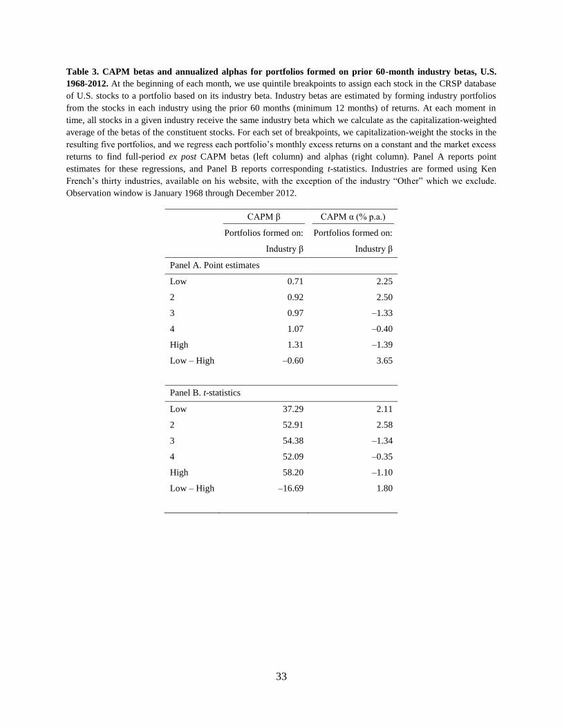
The low risk anomaly across industries. Table 3 is a prelude to the decomposition of

the low risk anomaly, repeating the analysis in the first and third columns of Table 1 with

industry betas in place of stock betas. A stock’s industry beta is the beta of the capitalization-

weighted average of the betas of the stocks within the industry: on each estimation date, the

14

industry beta is the same for each stock in a given industry. Each month, we use quintile

breakpoints to assign an approximately equal number of stocks to each of five portfolios using

industry betas. All stocks in a given industry are assigned to a single quintile portfolio. We again

capitalization-weight the stocks in each portfolio to find portfolio returns, and we estimate

market betas and CAPM alphas. The first column suggests that historic, ex ante industry beta is

able to predict ex post realized stock betas, but not as well as historic stock betas. In this column,

the difference between the ex post betas of the high and low portfolios is –0.60, with a t-statistic

of –16.69, roughly two-thirds of the spread achieved using stock betas in Table 1. Similarly,

compared to the difference in ex post alphas using stocks’ own betas, the second column reports

a smaller and marginally significant difference in ex post alphas of 3.65%, with a t-statistic of

1.80. In short, using only information about industry betas and no stock level information

delivers a reasonable fraction of the risk reduction and risk-adjusted return improvement of stock

level sorts.

Decomposing the low risk anomaly between stocks and industries. We now turn to

the main question: To what degree do macro effects contribute to the low risk anomaly? In this

case, industries represent the macro dimension of the anomaly. To understand the separate

contributions of industry selection and stock selection within industries, we combine the

independent quintile sorts of Table 1 and Table 3 into a double sort methodology. Each month,

we use independent quintile breakpoints to assign each stock to a portfolio based on its own beta

and its industry beta. We capitalization-weight the stocks in the resulting 25 portfolios.

We are interested in the contribution of stock level risk measures, once industry risk has

been taken into account, and we are interested in the contribution of industry level risk measures,

once stock level risk has been taken into account. We can only answer these questions to the

15

extent that these sorts do not lead to the same exact division of the CRSP sample. Figure 2 plots

the fraction of stocks in each of the resulting 25 portfolios in Panel A and the fraction of market

capitalization in Panel B. If these sorts led to the same division of the CRSP sample, all of the

firms and the market capitalization would lie on the diagonal. The plots show that the two effects

overlap considerably, especially when measured in terms of market capitalization. This is

intuitive, as large capitalization firms are likely to have measures of risk that are closer to the

capitalization-weighted industry beta. The plots also show that we will have some ability to

separate the two effects.

As a side note, we have also considered dependent sorts, in addition to the independent

sorts described below. We first sort stocks into quintiles using industry beta. Within each

quintile, we then sort using stock level beta. This forces an equal number of stocks into each of

the 25 portfolios. Our findings are largely similar using this approach, for both industries and the

country analysis described below.

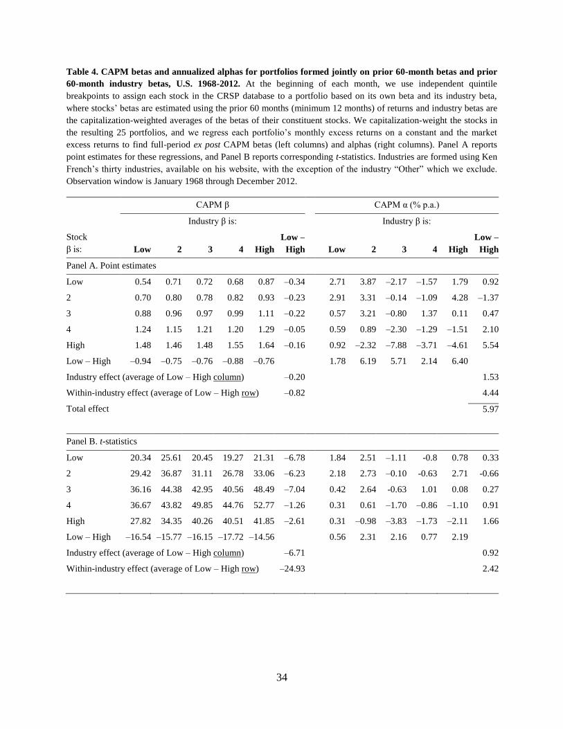
For each of the 25 independent double-sorted portfolios, we estimate an ex post beta and

CAPM alpha over the full period. Table 4 reports results. The left columns report betas, and the

right columns report alphas. In the left columns, betas are widely dispersed and tend to increase

from top to bottom and from left to right. For example, the first data column reports the betas of

portfolios formed from stocks in low-beta industries: reading down the column, portfolio betas

increase monotonically from 0.54 to 1.48 within this subsample. Similarly, the fifth data column

reports betas of portfolios formed from stocks in high-beta industries, and the range of portfolio

betas within this subsample also is large, increasing from 0.87 to 1.64. By contrast, rows display

much less variation in portfolio betas. For example, the “Low” row, which forms portfolios from

stocks with the lowest betas, shows that betas range from 0.54 to 0.87 for stocks in the lowest

16

and highest beta industries. Among high risk stocks in the “High” row, the industry effect is even

smaller. In this subsample, stocks in the highest-beta industries have an average beta of 1.64

compared to an average beta of 1.48 for stocks in the lowest-beta industries.

The statistics at the bottom of the panel summarize these patterns. The first is a pure

industry effect, measured as the average of the differences between high beta and low beta

industries, controlling for stock-level risk. This is the average of the differences reported in the

“Low – High” column. The second is a pure stock effect, measured as the average of the

differences between high beta and low beta stocks, controlling for industry risk. Again, this is the

average of the differences reported in the “Low – High” row. Our ability to find low risk

portfolios through the selection of low risk stocks within industries, at a –0.82 reduction in beta,

is about four times as large as our ability to find low risk portfolios through the selection of low

risk industries within stock risk groups. These results are consistent with stock level beta, as

estimated from historical data, being a much better predictor of future beta than industry beta.

However, both a stock level historical beta and its industry level historical beta, each relative to

the other, have incremental predictive power for future beta.

The t-statistics in Table 4 are computed taking into account the empirical covariance

among the 25 double-sorted portfolios. To be specific, we use a seemingly unrelated regression

model that allows regression errors to be contemporaneously correlated among the 25

regressions, but that assumes zero autocorrelations or cross-autocorrelations. Measures of risk

and differences in risk are highly statistically significant. Differences in return are harder to

detect in the data.

17

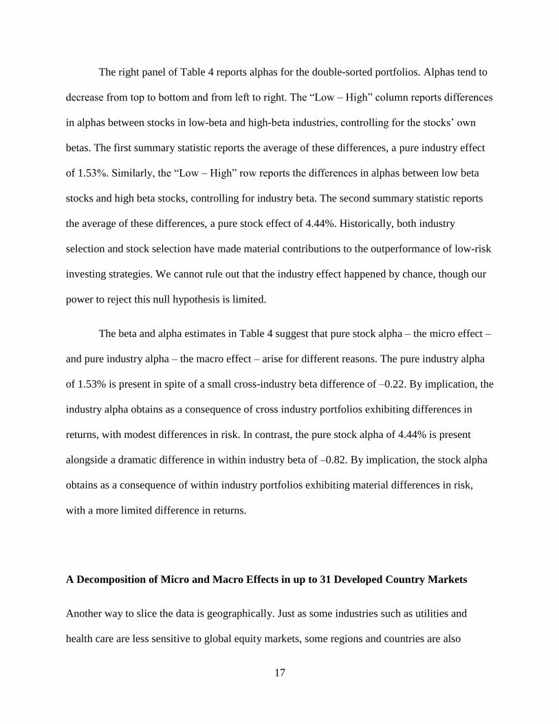
The right panel of Table 4 reports alphas for the double-sorted portfolios. Alphas tend to

decrease from top to bottom and from left to right. The “Low – High” column reports differences

in alphas between stocks in low-beta and high-beta industries, controlling for the stocks’ own

betas. The first summary statistic reports the average of these differences, a pure industry effect

of 1.53%. Similarly, the “Low – High” row reports the differences in alphas between low beta

stocks and high beta stocks, controlling for industry beta. The second summary statistic reports

the average of these differences, a pure stock effect of 4.44%. Historically, both industry

selection and stock selection have made material contributions to the outperformance of low-risk

investing strategies. We cannot rule out that the industry effect happened by chance, though our

power to reject this null hypothesis is limited.

The beta and alpha estimates in Table 4 suggest that pure stock alpha – the micro effect –

and pure industry alpha – the macro effect – arise for different reasons. The pure industry alpha

of 1.53% is present in spite of a small cross-industry beta difference of –0.22. By implication, the

industry alpha obtains as a consequence of cross industry portfolios exhibiting differences in

returns, with modest differences in risk. In contrast, the pure stock alpha of 4.44% is present

alongside a dramatic difference in within industry beta of –0.82. By implication, the stock alpha

obtains as a consequence of within industry portfolios exhibiting material differences in risk,

with a more limited difference in returns.

A Decomposition of Micro and Macro Effects in up to 31 Developed Country Markets

Another way to slice the data is geographically. Just as some industries such as utilities and

health care are less sensitive to global equity markets, some regions and countries are also

18

thought to have different risk properties. Japan, for example, has a low correlation with global

equity markets in its recent history. Next, we turn to decomposing the low risk anomaly into

country and stock effects.

Developed BMI includes Australia, Austria, Belgium, Canada, Denmark, Finland,

France, Germany, Hong Kong, Ireland, Italy, Japan, the Netherlands, New Zealand, Norway,

Singapore, Spain, Sweden, Switzerland, the United Kingdom, and the United States in the

sample of developed markets. In addition, several more countries are included or excluded at

some point during the sample. To avoid any lookahead bias, we follow the point-in-time S&P

decisions and include these countries in the developed market sample whenever S&P labels them

as such. These are the Czech Republic, Greece, Hungary, Iceland, Israel, Luxembourg, Malaysia,

Portugal, Slovenia, and South Korea. Each month and for each stock we estimate a stock beta

with respect to the global equity market using the previous 60 weeks of returns, measured from

Wednesday to Wednesday. Stocks with a shorter history than 60 weeks are included if they have

at least 12 weeks of returns. We define the global equity market as the capitalization-weighted

average return of the entire BMI developed market sample. We also measure an analogous

country beta. Each stock is mapped to a country, and the stock's country beta is the

capitalization-weighted average of the betas of each stock within the country: on each estimation

date, the country beta is the same for each stock in a given country.

The low risk anomaly across countries. In what follows, we repeat the industry analysis

for countries in the BMI sample. As before, Table 5 is a prelude to the decomposition of the low

risk anomaly, repeating the analysis in the second and fourth columns of Table 1 with country

betas in place of stock betas. The first column suggests that historic, ex ante country beta is able

to predict ex post realized stock betas, but like industries not as well as historic stock betas. In

19

this column, the difference between the ex post betas of the high and low portfolios is

–0.55, with a t-statistic of –8.78, roughly half of the spread achieved using stock betas in Table 1.

The alpha differences are somewhat stronger than industry sorts. The second column shows a

difference in ex post alphas that is smaller than Table 1, but still reasonably large at 6.86 with a

t-statistic of 1.97. In short, using only information about country betas and no stock level

information delivers roughly half the risk reduction and about two-thirds of the risk-adjusted

return improvement of stock level sorts. This combination of a substantial risk-adjusted return

difference and lower risk reduction is a preview of the decomposition. As we will see, unlike the

industry analysis, there is something extra in the country beta sorts, in terms of total returns, that

is not captured in the stock beta sorts of Table 1.

Decomposing the low risk anomaly between stocks and countries. We now ask to

what degree macro effects contribute to the low risk anomaly, but, in this case, countries

represent the macro dimension of the anomaly. To understand the separate contributions of

country selection and stock selection within countries, we repeat the independent quintile sorts of

Table 4 in Table 6. Each month, we use independent quintile breakpoints to assign each stock to

a portfolio based on its own beta and its country beta. We capitalization-weight the stocks in the

resulting 25 portfolios.

We are interested in the contribution of stock level risk measures, once country risk has

been taken into account, and we are interested in the contribution of country level risk measures,

once stock level risk has been taken into account. We can only answer these questions to the

extent that these sorts do not lead to the same exact division of the BMI sample. Figure 3 plots

the fraction of stocks in each of the resulting 25 portfolios in Panel A and the fraction of market

capitalization in Panel B. If these sorts led to the same division of the BMI sample, all of the

20

firms and the market capitalization would lie on the diagonal. The plots again show that the two

effects overlap considerably, especially when measured in terms of market capitalization.

For each of the 25 independent double-sorted portfolios, we estimate an ex post beta and

CAPM alpha over the full period. In Table 6, the left columns report betas, and the right columns

report alphas. In the left columns, betas are widely dispersed and tend to increase from top to

bottom and from left to right. For example, the first data column reports the betas of portfolios

formed from stocks in low-beta countries: reading down the column, portfolio betas range from

0.52 to 1.62 within this subsample. Similarly, the fifth data column reports betas of portfolios

formed from stocks in high-beta countries, and the range of portfolio betas within this subsample

also is large, from 0.65 to 1.67. By contrast, rows display even less variation in portfolio betas

than industry sorts delivered. For example, the “Low” row, which forms portfolios from stocks

with the lowest betas, shows that betas range from 0.52 to 0.65 for stocks in the lowest and

highest beta countries.

The statistics at the bottom of the panel summarize these patterns. The first is a pure

country effect, measured as the average of the differences between high beta and low beta

countries, controlling for stock-level risk. The second is a pure stock effect, measured as the

average of the differences between high beta and low beta stocks, controlling for country risk.

Our ability to find low risk portfolios through the selection of low risk stocks within countries, at

a –1.01 reduction in beta, is 50 times as large as our ability to find low risk portfolios through the

selection of low risk countries within stock risk groups. These results are consistent with stock

level beta, as estimated from historical data, being a much better predictor of future beta than its

country beta. This time the incremental predictive power of country level historical beta is closer

to zero, in both economic and statistical terms.

21

The right panel of Table 1 reports alphas for the double-sorted portfolios. Alphas tend to

decrease from top to bottom and from left to right. The average of these differences within each

row is a pure country effect of 6.22%. The average of these differences within each column is a

pure stock effect of 5.40%. Both are statistically significant at the 10% level. That is, historical

data suggest the low risk anomaly is present both within and across countries.

In short, the same picture emerges with countries as we saw with industries. The beta and

alpha estimates in Table 6 suggest that pure stock alpha – the micro effects – and pure country

alpha – the macro effect – arise for different reasons. The pure country alpha of 6.22% is present

in spite of no cross-country beta difference. By implication, the country alpha obtains as a

consequence of cross country portfolios exhibiting material differences in returns, with modest

differences in risk. In contrast, the pure stock alpha of 5.40% is present alongside a dramatic

difference in within country beta of –1.01. By implication, the stock alpha obtains as a

consequence of within country portfolios exhibiting material differences in risk, with modest

differences in returns.

Idiosyncratic Risk

The same analysis can be done with idiosyncratic risk instead of beta. But, the process

requires a bit more decision making. In particular, the industry contribution could be measured

with the idiosyncratic risk of aggregated industry portfolios, or it could be measured with the

average of firm-level idiosyncratic risk within the industry. The first measures the risk of the

industry, the other measures how risky the stocks are within the industry. We opt for the second

approach for both practical and theoretical reasons. Practically, our intuition is that the

22

idiosyncratic volatility of the industry average portfolio would perhaps be lower than all of the

individual stocks, because of the benefits of diversification, and it might be mechanically related

to the number of firms within each industry or country. Theoretically, we view the demand

arising at the stock level, so that an industry with lots of high risk stocks generates more

aggregate demand than an industry with few.

This foreshadows what we find in the data. We repeat Table 4 and Table 6 using

idiosyncratic risk instead of beta, and we show the summary results in Table 7. The first row of

each panel is a pure industry effect or a pure country effect, measured as the average of the

differences between high and low idiosyncratic risk industries and countries, controlling for

stock-level idiosyncratic risk. The second row of each panel is a pure stock effect, measured as

the average of the differences between high and low idiosyncratic risk stocks, controlling for

industry or country idiosyncratic risk. What we find is that the idiosyncratic risk effect is almost

entirely a micro phenomenon. 96% comes from a pure stock effect in the CRSP industry sample.

86% comes from a pure stock effect in the BMI country sample. Idiosyncratic risk is like

valuation ratios, in the sense that the intuition does not necessarily aggregate. What matters is

whether a stock is risky relative to a stock in its category more than the category average.

Conclusion: Samuelson’s Dictum and the Implications for Managed Volatility Strategies

The decomposition of the low risk anomaly has both theoretical and practical implications. The

superior performance of lower risk stocks that is evident in Figure 1 in both U.S. and

international markets is a very basic form of market inefficiency. It has both micro and macro

components. The micro component arises from the selection of lower risk stocks, holding

23

country and industry risk constant. The macro component arises from the selection of lower risk

industries and countries, holding stock level risk constant.

In theory, market inefficiency arises from some combination of less than fully rational

demand and the limits to arbitrage. Shiller (2001) has attributed to Samuelson the hypothesis that

macro inefficiencies are quantitatively larger than micro efficiencies. In contrast, we find that the

contribution to the low risk anomaly is of similar magnitude across micro and macro effects.

While stock selection leads to higher alpha through a combination of significant risk reduction

with modest return improvements, country selection leads to higher alpha through a combination

of significant return improvements and modest risk reduction. Industry selection is relatively

modest and the extra alpha cannot be distinguished from zero statistically. We view this as

affirmation of a modified version of Samuelson’s dictum. Namely, micro efficiency holds only

up to the limits of arbitrage. The constraint of fixed benchmark mandates makes low risk stocks

unattractive to many institutional investors. Macro inefficiency is present for countries more so

than for industries, perhaps because arbitrage is more limited across countries than across

industries.

The absence of material risk reduction from the macro selection of industries and

countries suggests two things. The first is that pure country or industry risk prediction is hard,

compared to predicting the relative risk of individual stocks. The second is that, to the extent this

anomaly arises because of investor demand for high risk aggregations of stocks, this demand is

in large part backward looking. The pattern of returns suggests that behavioral demand tilts

towards sectors and countries that have experienced relatively higher risk in the past.

24

In practice, the incremental value of industry and country selection, even holding stock

level risk constant, suggests that the use of a risk model in beta estimation that includes fixed

country and industry effects is preferable to simple stock level sorts on beta or volatility. This

has been especially true in global portfolios, where the incremental value of estimating country

level risk was significant. Moreover, because country and industry exposures have generated

incremental alpha, a global mandate with somewhat relaxed country and industry constraints

would have delivered higher risk-adjusted returns.

We thank Ely Spears and Adoito Haroon for excellent research assistance. Baker gratefully

acknowledges the Division of Research of the Harvard Business School for financial support.

25

References

Ahearne, Alan, William Griever, and Francis Warnock. 2004. “Information Costs and Home

Bias: An Analysis of US Holdings of Foreign Equities.” Journal of International Economics,

vol. 62, no. 2 (July):313–336.

Ang, Andrew, Robert J. Hodrick, Yuhang Xing, and Xiaoyan Zhang. 2006. “The Cross-Section

of Volatility and Expected Returns.” Journal of Finance, vol. 61, no. 1 (February):259-299.

Ang, Andrew, Robert J. Hodrick, Yuhang Xing, and Xiaoyan Zhang. 2009. “High Idiosyncratic

Volatility and Low Returns: International and Further U.S. Evidence.” Journal of Financial

Economics, vol. 91, no. 1 (January):1-23.

Asness, Cliff, Andrea Frazzini, and Lasse H. Pedersen. 2013. “Low-Risk Investing without

Industry Bets.” Working paper, AQR Capital Management (May).

Baker, Malcolm, Brendan Bradley, and Jeffrey Wurgler. 2011. “Benchmarks as Limits to

Arbitrage: Understanding the Low-Volatility Anomaly.” Financial Analysts Journal, vol. 67,

no. 1 (January/February):40-54.

Baker, Nardin, and Robert A. Haugen. 2012. “Low Risk Stocks Outperform within All

Observable Markets of the World.” SSRN Working Paper 205543 (April).

Bali, Turan, Nusret Cakici, and Robert F. Whitelaw. 2011. “Maxing Out: Stocks as Lotteries and

the Cross-Section of Expected Returns.” Journal of Financial Economics, vol. 99, no. 2

(February):427-446.

Basu, S. 1977. “Investment Performance of Common Stocks in Relation to Their Price-Earnings

Ratios: A Test of Market Efficiency.” Journal of Finance, vol. 32, no. 3 (June):663-682.

Black, Fischer. 1972. “Capital Market Equilibrium with Restricted Borrowing.” Journal of

Business, vol. 45, no. 3 (July):444-455.

Black, Fischer, Michael C. Jensen, and Myron Scholes. 1972. “The Capital Asset Pricing Model:

Some Empirical Tests.” In Studies in the Theory of Capital Markets. Edited by Michael C.

Jensen. New York: Praeger.

Blitz, David, Juan Pang and Pim van Vliet. 2012. “The Volatility Effect in Emerging Markets.”

SSRN Working Paper 2050863 (April).

Brennan, Michael. 1993. “Agency and Asset Pricing.” Working paper, University of California,

Los Angeles (May).

Campbell, John. 1991. “A Variance Decomposition for Stock Returns.” Economic Journal, vol.

101, no. 405 (March):157–79.

26

Daniel, Kent, and Moskowitz, Tobias. 2013. “Momentum Crashes.” Working paper, Columbia

University (April).

Falkenstein, Eric. 1994. “Mutual Funds, Idiosyncratic Variance, and Asset Returns.”

Dissertation, Northwestern University.

Fama, Eugene F., and Kenneth R. French. 1992. “The Cross-Section of Expected Stock

Returns.” Journal of Finance, vol. 47, no. 2 (June):427-465.

Fama, Eugene F., and Kenneth R. French. 1997. “Industry Costs of Equity.” Journal of

Financial Economics, vol. 43, no. 2 (February):153–193.

Fama, Eugene F., and Kenneth R. French. 1998. “Value versus Growth: The International

Evidence.” Journal of Finance, vol. 53, no. 6 (December):1975-1999.

Frazzini, Andrea, and Lasse H. Pedersen. 2010. “Betting Against Beta.” Working paper, New

York University (May).

French, Kenneth R., and James Poterba. 1991. “Investor Diversification and International Equity

Markets.” American Economic Review, vol. 81, no. 2 (May):222-226.

Haugen, Robert A., and A. James Heins. 1975. “Risk and the Rate of Return on Financial Assets:

Some Old Wine in New Bottles.” Journal of Financial and Quantitative Analysis, vol. 10,

no. 5 (December):775-784.

Hong, Harrison, and David Sraer. 2012. “Speculative Betas.” Working paper, Princeton

University (August).

Jung, Jeeman, and Robert J. Shiller. 2005. “Samuelson’s Dictum and the Stock Market.”

Economic Inquiry, vol. 43, no. 2 (April):221–228.

Karceski, Jason. 2002. Returns-Chasing Behavior, Mutual Funds, and Beta’s Death.” Journal of

Financial and Quantitative Analysis, vol. 37, no. 4 (December):559–594.

Kothari, S. P., and Jay Shanken. 1997. “Book-to-Market, Dividend Yield, and Expected Market

Returns: A Time-Series Analysis.” Journal of Financial Economics, vol. 44, no. 2

(May):169-203.

Lamont, Owen, and Jeremy C. Stein. 2006. “Investor Sentiment and Corporate Finance: Micro

and Macro.” American Economic Review, vol. 96, no. 2 (May):147-151.

Lewellen, Jonathan. 1999. “The Time-Series Relations among Expected Return, Risk, and Book-

to-Market.” Journal of Financial Economics, vol. 54, no. 1 (October):5-43.

Li, Xi, Rodney Sullivan, and Luis Garcia-Feijoo. 2013. “The Limits to Arbitrage and the Low-

Volatility Anomaly.” Financial Analysts Journal, forthcoming.

27

Scholes, Myron. 1972. “The Market for Securities: Substitution versus Price Pressure and the

Effects of Information on Share Prices.” The Journal of Business, vol. 45, no. 2 (April):179-

211.

Samuelson, Paul. 1998. “Summing up on Business Cycles: Opening Address.” In Beyond

Shocks: What Causes Business Cycles. Edited by Jeffrey C. Fuhrer and Scott Schuh. Boston:

Federal Reserve Bank of Boston.

Shiller, Robert J. 2001. Irrational exuberance. New York: Broadway Books.

Vuolteenaho, Tuomo. 2002. “What Drives Firm-Level Stock Returns?” Journal of Finance, vol.

57, no. 1 (February):233– 64.

28

Figure 1. Cumulative returns of five portfolios formed on stocks’ prior betas for U.S. 1968-2012 and

developed markets 1989-2012. At the beginning of each month, we use quintile breakpoints to assign each stock in

the CRSP database (U.S., Panel A) and in S&P’s Broad Market Index (BMI) database (developed markets, Panel B)

to one of five portfolios based on its beta, estimated using the prior 60 (minimum 12) months (Panel A) or weeks

(Panel B) of returns. We capitalization-weight the stocks in the resulting five portfolios, and we plot the cumulative

returns of investing one U.S. dollar in each. In Panel B, countries included for the full sample are Australia, Austria,

Belgium, Canada, Denmark, Finland, France, Germany, Hong Kong, Ireland, Italy, Japan, the Netherlands, New

Zealand, Norway, Singapore, Spain, Sweden, Switzerland, the United Kingdom, and the United States; countries

included for part of the sample are the Czech Republic, Greece, Hungary, Iceland, Israel, Luxembourg, Malaysia,

Portugal, Slovenia, and South Korea. Betas are calculated with respect to the capitalization-weighted portfolio of

U.S. stocks using monthly returns (Panel A) and with respect to the capitalization-weighted portfolio of developed

market stocks using weekly returns (Panel B). All returns are measured in U.S. dollars. Returns greater than 1,000%

and less than –100% are excluded from the BMI database. Observation windows are January 1968 through

December 2012 (Panel A) and November 1989 through December 2012 (Panel B).

Panel A. Cumulative returns for five portfolios formed on U.S. stocks’ prior 60-month betas

Value of $1 invested in 1968

Panel B. Cumulative returns for five portfolios formed on developed market stocks’ prior 60-week betas

Value of $1 invested in 1989

Bottom Quintile

Top Quntile

0.1

1

10

100

1968 1972 1976 1980 1984 1988 1992 1996 2000 2004 2008 2012

Bottom Quintile

Top Quintile

0.1

1

10

100

1988 1992 1996 2000 2004 2008 2012

29

Figure 2. Distribution of stocks across portfolios formed jointly on stocks’ betas and their industry betas, U.S.

1968-2012. At the beginning of each month, we use independent quintile breakpoints to assign each stock in the

CRSP database to a portfolio based on its own beta and its industry’s beta, where stocks' betas estimated using the

prior 60 months (minimum 12 months) of returns and industry betas are the capitalization weighted average of the

industry constituent stock betas. Industries are formed using Ken French’s thirty industries, available on his website,

with the exception of the industry “Other” which we exclude. Vertical bars denote the time-series average fraction

of stocks (Panel A) or fraction of market capitalization (Panel B) in each portfolio. Observation window is January

1968 through December 2012.

Panel A. Average distribution of stocks across double-sorted portfolios

Panel B. Average distribution of market capitalization across double-sorted portfolios

0.00

0.05

0.10

Low2

34

High

Industry beta

Average fraction of stocks

Stock beta

0.00

0.05

0.10

Low2

34

High

Industry beta

Average fraction of market value

Stock beta

30

Figure 3. Distribution of stocks across portfolios formed jointly on stocks’ betas and their country betas,

developed markets 1989-2012. At the beginning of each month, we use independent quintile breakpoints to assign

each stock in the S&P Broad Market Index (BMI) developed markets database to a portfolio based on its own beta

and its country’s beta, where stocks’ betas are estimated using the prior 60 weeks (minimum 12 weeks) of returns

and country betas are the capitalization-weighted averages of the betas of constituent stocks, and where all returns

are measured in U.S. dollars. Returns greater than 1,000% and less than –100% are excluded. Vertical bars denote

the time-series average fraction of stocks (Panel A) or fraction of market capitalization (Panel B) in each portfolio.

Observation window is November 1989 through December 2012.

Panel A. Average distribution of stocks across double-sorted portfolios

Panel B. Average distribution of market capitalization across double-sorted portfolios

0.00

0.05

0.10

Low2

34

High

Country beta

Average fraction of stocks

Stock beta

0.00

0.05

0.10

Low2

34

High

Country beta

Average fraction of market value

Stock beta

31

Table 1. CAPM betas and annualized alphas for portfolios formed on stocks’ prior betas. We source data from

CRSP from January 1968 through December 2012 and from S&P BMI from November 1989 through December

2012. At the beginning of each month, we use quintile breakpoints to assign each stock to a portfolio based on its

own beta. Betas in the CRSP sample are estimated using the prior 60 months (minimum 12 months) of returns. Betas

in the BMI sample are estimated using the prior 60 weeks (minimum 12 weeks) of returns, where all returns are

measured in U.S dollars. For each set of breakpoints, we capitalization-weight the stocks in the resulting five

portfolios, and we regress each portfolio’s monthly excess returns on a constant and the market excess returns to

find full-period ex post CAPM betas (left columns) and alphas (right columns). To compute excess returns, we use

the U.S. government one-month (T-bill) rate as the risk-free rate. Panel A reports point estimates for these

regressions, and Panel B reports corresponding t-statistics. Countries included for the full sample are Australia,

Austria, Belgium, Canada, Denmark, Finland, France, Germany, Hong Kong, Ireland, Italy, Japan, the Netherlands,

New Zealand, Norway, Singapore, Spain, Sweden, Switzerland, the United Kingdom, and the United States;

countries included for part of the sample are the Czech Republic, Greece, Hungary, Iceland, Israel, Luxembourg,

Malaysia, Portugal, Slovenia, and South Korea. Returns greater than 1,000% and less than

–100% are excluded. For CRSP, the market portfolio is from Ken French’s web site. For BMI, the market portfolio

is the capitalization-weighted portfolio of all included stocks.

CAPM β CAPM α (% p.a.)

Portfolios formed on: Portfolios formed on:

CRSP

Stock β

BMI

Stock β

CRSP

Stock β

BMI

Stock β

Panel A. Point estimates

Low 0.59 0.47 2.27 3.74

2 0.76 0.69 2.10 3.60

3 0.98 0.88 0.28 2.01

4 1.24 1.16 –1.52 –1.32

High 1.61 1.69 –4.49 –5.50

Low – High –1.02 –1.22 6.76 9.24

Panel B. t-statistics

Low 31.24 18.42 2.16 2.62

2 49.56 30.98 2.45 2.92

3 72.75 46.05 0.37 1.89

4 85.93 69.22 –1.89 –1.42

High 54.09 41.95 –2.70 –2.45

Low – High –23.99 –19.89 2.84 2.71

32

Table 2. CAPM annualized alphas for portfolios formed on stocks’ prior betas. We repeat the analysis in Table

1, using lagged values of beta. We source data from CRSP from January 1968 through December 2012. At the

beginning of each month, we use quintile breakpoints to assign each stock to a portfolio based on its own beta. Betas

in the CRSP sample are estimated using the prior 60 months (minimum 12 months) of returns. For each set of

breakpoints, we capitalization-weight the stocks in the resulting five portfolios, and we regress each portfolio’s

monthly excess returns on a constant and the market excess returns to find full-period ex post CAPM alphas. To

compute excess returns, we use the U.S. government one-month (T-bill) rate as the risk-free rate. Panel A reports

point estimates for these regressions, and Panel B reports corresponding t-statistics.

CAPM α (% p.a.)

Portfolios formed on:

CRSP

Stock β

CRSP t-2

Stock β

CRSP t-3

Stock β

CRSP t-12

Stock β

Panel A. Point estimates

Low 2.27 2.29 1.82 2.00

2 2.10 1.80 1.66 1.87

3 0.28 0.27 0.26 0.05

4 –1.52 -1.34 -1.06 -0.98

High –4.49 -4.81 -4.65 -3.57

Low – High 6.76 7.10 6.48 5.58

Panel B. t-statistics

Low 2.16 2.20 1.72 1.92

2 2.45 2.10 1.95 2.22

3 0.37 0.37 0.34 0.06

4 –1.89 -1.69 -1.36 -1.32

High –2.70 -2.98 -2.86 -2.36

Low – High 2.84 3.05 2.76 2.52

33

Table 3. CAPM betas and annualized alphas for portfolios formed on prior 60-month industry betas, U.S.

1968-2012. At the beginning of each month, we use quintile breakpoints to assign each stock in the CRSP database

of U.S. stocks to a portfolio based on its industry beta. Industry betas are estimated by forming industry portfolios

from the stocks in each industry using the prior 60 months (minimum 12 months) of returns. At each moment in

time, all stocks in a given industry receive the same industry beta which we calculate as the capitalization-weighted

average of the betas of the constituent stocks. For each set of breakpoints, we capitalization-weight the stocks in the

resulting five portfolios, and we regress each portfolio’s monthly excess returns on a constant and the market excess

returns to find full-period ex post CAPM betas (left column) and alphas (right column). Panel A reports point

estimates for these regressions, and Panel B reports corresponding t-statistics. Industries are formed using Ken

French’s thirty industries, available on his website, with the exception of the industry “Other” which we exclude.

Observation window is January 1968 through December 2012.

CAPM β CAPM α (% p.a.)

Portfolios formed on: Portfolios formed on:

Industry β Industry β

Panel A. Point estimates

Low 0.71 2.25

2 0.92 2.50

3 0.97 –1.33

4 1.07 –0.40

High 1.31 –1.39

Low – High –0.60 3.65

Panel B. t-statistics

Low 37.29 2.11

2 52.91 2.58

3 54.38 –1.34

4 52.09 –0.35

High 58.20 –1.10

Low – High –16.69 1.80

34

Table 4. CAPM betas and annualized alphas for portfolios formed jointly on prior 60-month betas and prior

60-month industry betas, U.S. 1968-2012. At the beginning of each month, we use independent quintile

breakpoints to assign each stock in the CRSP database to a portfolio based on its own beta and its industry beta,

where stocks’ betas are estimated using the prior 60 months (minimum 12 months) of returns and industry betas are

the capitalization-weighted averages of the betas of their constituent stocks. We capitalization-weight the stocks in

the resulting 25 portfolios, and we regress each portfolio’s monthly excess returns on a constant and the market

excess returns to find full-period ex post CAPM betas (left columns) and alphas (right columns). Panel A reports

point estimates for these regressions, and Panel B reports corresponding t-statistics. Industries are formed using Ken

French’s thirty industries, available on his website, with the exception of the industry “Other” which we exclude.

Observation window is January 1968 through December 2012.

CAPM β CAPM α (% p.a.)

Industry β is: Industry β is:

Stock

β is: Low 2 3 4 High

Low –

High Low 2 3 4 High

Low –

High

Panel A. Point estimates

Low 0.54 0.71 0.72 0.68 0.87 –0.34 2.71 3.87 –2.17 –1.57 1.79 0.92

2 0.70 0.80 0.78 0.82 0.93 –0.23 2.91 3.31 –0.14 –1.09 4.28 –1.37

3 0.88 0.96 0.97 0.99 1.11 –0.22 0.57 3.21 –0.80 1.37 0.11 0.47

4 1.24 1.15 1.21 1.20 1.29 –0.05 0.59 0.89 –2.30 –1.29 –1.51 2.10

High 1.48 1.46 1.48 1.55 1.64 –0.16 0.92 –2.32 –7.88 –3.71 –4.61 5.54

Low – High –0.94 –0.75 –0.76 –0.88 –0.76 1.78 6.19 5.71 2.14 6.40

Industry effect (average of Low – High column) –0.20 1.53

Within-industry effect (average of Low – High row) –0.82 4.44

Total effect 5.97

Panel B. t-statistics

Low 20.34 25.61 20.45 19.27 21.31 –6.78 1.84 2.51 –1.11 -0.8 0.78 0.33

2 29.42 36.87 31.11 26.78 33.06 –6.23 2.18 2.73 –0.10 -0.63 2.71 -0.66

3 36.16 44.38 42.95 40.56 48.49 –7.04 0.42 2.64 -0.63 1.01 0.08 0.27

4 36.67 43.82 49.85 44.76 52.77 –1.26 0.31 0.61 –1.70 –0.86 –1.10 0.91

High 27.82 34.35 40.26 40.51 41.85 –2.61 0.31 –0.98 –3.83 –1.73 –2.11 1.66

Low – High –16.54 –15.77 –16.15 –17.72 –14.56 0.56 2.31 2.16 0.77 2.19

Industry effect (average of Low – High column) –6.71 0.92

Within-industry effect (average of Low – High row) –24.93 2.42

35

Table 5. CAPM betas and annualized alphas for portfolios formed on prior 60-week country betas, developed

markets 1989-2012. At the beginning of each month, we use quintile breakpoints to assign each stock in the S&P

Broad Market Index (BMI) developed markets database to a portfolio based on its country beta. Country betas are

the capitalization-weighted averages of constituent stocks’ betas, which are estimated using the prior 60 weeks

(minimum 12 weeks) of returns, where all returns are measured in U.S. dollars. For each set of breakpoints, we

capitalization-weight the stocks in the resulting five portfolios, and we regress each portfolio’s monthly excess

returns on a constant and the market excess returns to find full-period ex post CAPM betas (left columns) and alphas

(right columns). Panel A reports point estimates for the regressions, and Panel B reports corresponding t-statistics.

Observation window is November 1989 through December 2012.

CAPM β CAPM α (% p.a.)

Portfolios formed on: Portfolios formed on:

Country β Country β

Panel A. Point estimates

Low 0.77 5.87

2 0.86 4.77

3 0.99 0.78

4 1.12 –1.49

High 1.32 –0.99

Low – High –0.55 6.86

Panel B. t-statistics

Low 21.71 2.97

2 27.05 2.68

3 31.81 0.45

4 33.49 –0.80

High 30.15 –0.41

Low – High –8.78 1.97

36

Table 6. CAPM betas and annualized alphas for portfolios formed jointly on prior 60-week betas and prior

60-week country betas, developed markets 1989-2012. At the beginning of each month, we use independent

quintile breakpoints to assign each stock in the S&P Broad Market Index (BMI) developed markets database to a

portfolio based on its own beta and its country beta, where stock betas are estimated using the prior 60 weeks

(minimum 12 weeks) of returns and country betas are the capitalization-weighted averages of the betas of

constituent stocks, and where all returns are measured in U.S. dollars. We capitalization-weight the stocks in the

resulting 25 portfolios, and we regress each portfolio’s monthly excess returns on a constant and the market excess

returns to find full-period ex post CAPM betas (left columns) and alphas (right columns). Panel A reports point

estimates for the regressions, and Panel B reports corresponding t-statistics. Observation window is November 1989

through December 2012.

CAPM β CAPM α (% p.a.)

Country β is: Country β is:

Stock

β is: Low 2 3 4 High

Low –

High Low 2 3 4 High

Low –

High

Panel A. Point estimates

Low 0.52 0.52 0.64 0.62 0.65 –0.13 5.49 6.27 1.97 0.16 –3.62 9.11

2 0.74 0.71 0.79 0.83 0.78 –0.04 7.55 6.77 3.51 0.71 –2.94 10.48

3 0.97 0.88 0.96 0.99 0.93 0.03 2.68 6.94 2.29 0.60 0.09 2.59

4 1.17 1.1 1.14 1.19 1.09 0.08 2.60 2.00 0.11 –2.35 –0.69 3.29

High 1.62 1.59 1.62 1.51 1.67 –0.06 0.87 –0.39 –3.73 –8.71 –4.74 5.61

Low – High –1.09 –1.07 –0.98 –0.89 –1.02 4.62 6.66 5.7 8.88 1.11

Country effect (average of Low – High column) –0.02 6.22

Within-country effect (average of Low – High row) –1.01 5.40

Total effect 11.61

Panel B. t-statistics

Low 14.35 12.29 13.27 12.62 10.41 –1.94 2.71 2.7 0.74 0.06 –1.04 2.45

2 18.87 19.40 21.71 18.83 15.77 –0.78 3.47 3.33 1.74 0.29 –1.07 3.43

3 21.58 21.79 28.00 25.07 19.94 0.54 1.08 3.11 1.21 0.27 0.04 0.73

4 19.17 22.63 32.45 30.56 23.93 1.07 0.77 0.74 0.06 –1.09 –0.27 0.78

High 15.39 21.62 26.71 23.22 27.52 –0.50 0.15 –0.10 –1.11 –2.41 –1.40 0.88

Low – High –10.08 –12.75 –13.74 –12.01 –12.98 0.77 1.43 1.45 2.16 0.26

Country effect (average of Low – High column) –0.42 2.04

Within-country effect (average of Low – High row) –17.95 1.73

37

Table 7. CAPM betas and annualized alphas for portfolios formed jointly on prior 60-month idiosyncratic

volatility and prior industry and country idiosyncratic volatility. Panels A and B repeat the analysis in Tables 4

and 6, respectively, using the volatility of the residual from the CAPM regressions described there, instead of the

beta. Specifically, at the beginning of each month, we use independent quintile breakpoints to assign each stock in

the CRSP (BMI) database to a portfolio based on its own idiosyncratic volatility and its industry (country)

idiosyncratic volatility, where stocks’ idiosyncratic volatiles are estimated using the prior 60 months (weeks) of

returns and industry (country) idiosyncratic volatiles are the capitalization-weighted averages of the idiosyncratic

volatiles of their constituent stocks. We capitalization-weight the stocks in the resulting 25 portfolios, and we

regress each portfolio’s monthly excess returns on a constant and the market excess returns to find full-period ex

post CAPM betas (left columns) and alphas (right columns). We report the average differences between low and

high idiosyncratic risk industries (countries) controlling for stock-level idiosyncratic risk as the “industry effect”

(“country effect”), and we report the average differences between low and high idiosyncratic risk stocks controlling

for industry (country) idiosyncratic volatility as the “within-industry” (“within-country”) effect. Estimation window

is 1968-2012 (CRSP, Panel A) and 1989-2012 (BMI, Panel B).

CAPM β CAPM α (% p.a.)

Point Estimate T-Stat Point Estimate T-Stat

Panel A. CRSP Sample

Industry effect –0.22 –6.31 0.42 0.22

Within-industry effect –0.73 –14.39

10.21 3.59

Total effect 10.63

Panel B. BMI Sample

Country effect 0.03 0.43 1.54 0.42

Within-country effect –0.78 –12.66 9.72 2.82

Total effect 11.26