The LOCO-I Lossless Image Compression Algorithm:

Principles and Standardization into JPEG-LS

Marcelo J. Weinberger and Gadiel Seroussi

Hewlett-Packard Laboratories, Palo Alto, CA 94304, USA

Guillermo Sapiro�

Department of Electrical and Computer Engineering

University of Minnesota, Minneapolis, MN 55455, USA.

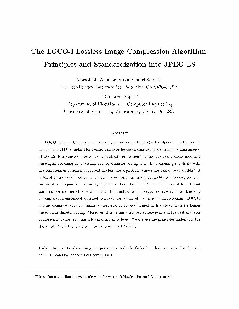
Abstract

LOCO-I (LOw COmplexity LOssless COmpression for Images) is the algorithm at the core of

the new ISO/ITU standard for lossless and near-lossless compression of continuous-tone images,

JPEG-LS. It is conceived as a \low complexity projection" of the universal context modeling

paradigm, matching its modeling unit to a simple coding unit. By combining simplicity with

the compression potential of context models, the algorithm \enjoys the best of both worlds." It

is based on a simple �xed context model, which approaches the capability of the more complex

universal techniques for capturing high-order dependencies. The model is tuned for e�cient

performance in conjunction with an extended family of Golomb-type codes, which are adaptively

chosen, and an embedded alphabet extension for coding of low-entropy image regions. LOCO-I

attains compression ratios similar or superior to those obtained with state-of-the-art schemes

based on arithmetic coding. Moreover, it is within a few percentage points of the best available

compression ratios, at a much lower complexity level. We discuss the principles underlying the

design of LOCO-I, and its standardization into JPEG-LS.

Index Terms: Lossless image compression, standards, Golomb codes, geometric distribution,

context modeling, near-lossless compression.

�This author's contribution was made while he was with Hewlett-Packard Laboratories.

1 Introduction

LOCO-I (LOw COmplexity LOssless COmpression for Images) is the algorithm at the core of

the new ISO/ITU standard for lossless and near-lossless compression of continuous-tone images,

JPEG-LS. The algorithm was introduced in an abridged format in [1]. The standard evolved after

successive re�nements [2, 3, 4, 5, 6], and a complete speci�cation can be found in [7]. However, the

latter reference is quite obscure, and it omits the theoretical background that explains the success

of the algorithm. In this paper, we discuss the theoretical foundations of LOCO-I and present a

full description of the main algorithmic components of JPEG-LS.

Lossless data compression schemes often consist of two distinct and independent components:

modeling and coding. The modeling part can be formulated as an inductive inference problem,

in which the data (e.g., an image) is observed sample by sample in some pre-de�ned order (e.g.,

raster-scan, which will be the assumed order for images in the sequel). At each time instant t,

and after having scanned past data xt = x1x2 � � � xt, one wishes to make inferences on the next

sample value xt+1 by assigning a conditional probability distribution P (�jxt) to it. Ideally, the

code length contributed by xt+1 is � logP (xt+1jxt) bits (hereafter, logarithms are taken to the

base 2), which averages to the entropy of the probabilistic model. In a sequential formulation, the

distribution P (�jxt) is learned from the past and is available to the decoder as it decodes the past

string sequentially. Alternatively, in a two-pass scheme the conditional distribution can be learned

from the whole image in a �rst pass and must be sent to the decoder as header information.1

The conceptual separation between the modeling and coding operations [9] was made possible

by the invention of the arithmetic codes [10], which can realize any probability assignment P (�j�),

dictated by the model, to a preset precision. These two milestones in the development of lossless

data compression allowed researchers to view the problem merely as one of probability assignment,

concentrating on the design of imaginative models for speci�c applications (e.g., image compression)

with the goal of improving on compression ratios. Optimization of the sequential probability

assignment process for images, inspired on the ideas of universal modeling, is analyzed in [11], where

a relatively high complexity scheme is presented as a way to demonstrate these ideas. Rather than

pursuing this optimization, the main objective driving the design of LOCO-I is to systematically

\project" the image modeling principles outlined in [11] and further developed in [12], into a

low complexity plane, both from a modeling and coding perspective. A key challenge in this

1A two-pass version of LOCO-I was presented in [8].

1

process is that the above separation between modeling and coding becomes less clean under the

low complexity coding constraint. This is because the use of a generic arithmetic coder, which

enables the most general models, is ruled out in many low complexity applications, especially for

software implementations.

Image compression models customarily consisted of a �xed structure, for which parameter

values were adaptively learned. The model in [11], instead, is adaptive not only in terms of the

parameter values, but also in structure. While [11] represented the best published compression

results at the time (at the cost of high complexity), it could be argued that the improvement

over the �xed model structure paradigm, best represented by the Sunset family of algorithms

[13, 14, 15, 16], was scant. The research leading to the CALIC algorithm [17], conducted in

parallel to the development of LOCO-I, seems to con�rm a pattern of diminishing returns. CALIC

avoids some of the optimizations performed in [11], but by tuning the model more carefully to

the image compression application, some compression gains are obtained. Yet, the improvement

is not dramatic, even for the most complex version of the algorithm [18]. More recently, the same

observation applies to the TMW algorithm [19], which adopts a multiple-pass modeling approach.

Actually, in many applications, a drastic complexity reduction can have more practical impact

than a modest increase in compression. This observation suggested that judicious modeling, which

seemed to be reaching a point of diminishing returns in terms of compression ratios, should rather

be applied to obtain competitive compression at signi�cantly lower complexity levels.

On the other hand, simplicity-driven schemes (e.g., the most popular version of the lossless

JPEG standard [20]) propose minor variations of traditional DPCM techniques [21], which include

Hu�man coding [22] of prediction residuals obtained with some �xed predictor. These simpler

techniques are fundamentally limited in their compression performance by the �rst order entropy

of the prediction residuals, which in general cannot achieve total decorrelation of the data [23]. The

compression gap between these simple schemes and the more complex ones is signi�cant, although

the FELICS algorithm [24] can be considered a �rst step in bridging this gap, as it incorporates

adaptivity in a low complexity framework.

While maintaining the complexity level of FELICS, LOCO-I attains signi�cantly better com-

pression ratios, similar or superior to those obtained with state-of-the art schemes based on arith-

metic coding, but at a fraction of the complexity. In fact, as shown in Section 6, when tested

over a benchmark set of images of a wide variety of types, LOCO-I performed within a few per-

2

centage points of the best available compression ratios (given, in practice, by CALIC), at a much

lower complexity level. Here, complexity was estimated by measuring running times of software

implementations made widely available by the authors of the respective algorithms.

In the sequel, our discussions will generally be con�ned to gray-scale images. For multi-

component (color) images, the JPEG-LS syntax supports both interleaved and non-interleaved

(i.e., component by component) modes. In interleaved modes, possible correlation between color

planes is used in a limited way, as described in the Appendix. For some color spaces (e.g., an RGB

representation), good decorrelation can be obtained through simple lossless color transforms as a

pre-processing step to JPEG-LS. Similar performance is attained by more elaborate schemes which

do not assume prior knowledge of the color space (see, e.g., [25] and [26]).

JPEG-LS o�ers a lossy mode of operation, termed \near-lossless," in which every sample value

in a reconstructed image component is guaranteed to di�er from the corresponding value in the

original image by up to a preset (small) amount, �. In fact, in the speci�cation [7], the lossless

mode is just a special case of near-lossless compression, with � = 0. This paper will focus mainly

on the lossless mode, with the near-lossless case presented as an extension in Section 4.

The remainder of this paper is organized as follows. Section 2 reviews the principles that

guide the choice of model in lossless image compression, and introduces the basic components of

LOCO-I as low complexity projections of these guiding principles. Section 3 presents a detailed

description of the basic algorithm behind JPEG-LS culminating with a summary of all the steps

of the algorithm. Section 4 discusses the near-lossless mode, while Section 5 discusses variations

to the basic con�guration, including one based on arithmetic coding, which has been adopted for

a prospective extension of the baseline JPEG-LS standard. In Section 6, compression results are

reported for standard image sets. Finally, an appendix lists various additional features in the

standard, including the treatment of color images.

While modeling principles will generally be discussed in reference to LOCO-I as the algorithm

behind JPEG-LS, speci�c descriptions will generally refer to LOCO-I/JPEG-LS, unless applicable

to only one of the schemes.

2 Modeling principles and LOCO-I

2.1 Model cost and prior knowledge

In this section, we review the principles that guide the choice of model and, consequently, the

resulting probability assignment scheme. In state-of-the-art lossless image compression schemes,

3

this probability assignment is generally broken into the following components:

a. A prediction step, in which a value x̂t+1 is guessed for the next sample xt+1 based on a �nite

subset (a causal template) of the available past data xt.

b. The determination of a context in which xt+1 occurs. The context is, again, a function of a

(possibly di�erent) causal template.

c. A probabilistic model for the prediction residual (or error signal) �t+1�= xt+1 � x̂t+1, condi-

tioned on the context of xt+1.

This structure was pioneered by the Sunset algorithm [13].

Model cost. A probability assignment scheme for data compression aims at producing a code

length which approaches the empirical entropy of the data. Lower entropies can be achieved

through higher order conditioning (larger contexts). However, this implies a larger number K of

parameters in the statistical model, with an associatedmodel cost [27] which could o�set the entropy

savings. This cost can be interpreted as capturing the penalties of \context dilution" occurring

when count statistics must be spread over too many contexts, thus a�ecting the accuracy of the

corresponding estimates. The per-sample asymptotic model cost is given by (K log n)=(2n), where

n is the number of data samples [28]. Thus, the number of parameters plays a fundamental role in

modeling problems, governing the above \tension" between entropy savings and model cost [27].

This observation suggests that the choice of model should be guided by the use, whenever possible,

of available prior knowledge on the data to be modeled, thus avoiding unnecessary \learning" costs

(i.e., over�tting). In a context model, K is determined by the number of free parameters de�ning

the coding distribution at each context and by the number of contexts.

Prediction. In general, the predictor consists of a �xed and an adaptive component. When the

predictor is followed by a zero-order coder (i.e., no further context modeling is performed), its

contribution stems from it being the only \decorrelation" tool. When used in conjunction with a

context model, however, the contribution of the predictor is more subtle, especially for its adaptive

component. In fact, prediction may seem redundant at �rst, since the same contextual information

that is used to predict is also available for building the coding model, which will eventually learn

the \predictable" patterns of the data and assign probabilities accordingly. The use of two di�erent

modeling tools based on the same contextual information is analyzed in [12], and the interaction is

also explained in terms of model cost. The �rst observation, is that prediction turns out to reduce

the number of coding parameters needed for modeling high order dependencies. This is due to the

4

existence of multiple conditional distributions that are similarly shaped but centered at di�erent

values. By predicting a deterministic, context-dependent value x̂t+1 for xt+1, and considering the

(context)-conditional probability distribution of the prediction residual �t+1 rather than that of xt+1

itself, we allow for similar probability distributions on �, which may now be all centered at zero, to

merge in situations when the original distributions on x would not. Now, while the �xed component

of the predictor can easily be explained as re ecting our prior knowledge of typical structures in

the data, leading, again, to model cost savings, the main contribution in [12] is to analyze the

adaptive component. Notice that adaptive prediction also learns patterns through a model (with

a number K 0 of parameters), which has an associated learning cost. This cost should be weighted

against the potential savings of O(K(logn)=n) in the coding model cost. A �rst indication that this

trade-o� might be favorable is given by the predictability bound in [29] (analogous to the coding

bound in [28]), which shows that the per-sample model cost for prediction is O(K 0=n), which is

asymptotically negligible with respect to the coding model cost. The results in [12] con�rm this

intuition and show that it is worth increasing K 0 while reducing K. As a result, [12] proposes the

basic paradigm of using a large model for adaptive prediction which in turn allows for a smaller

model for adaptive coding. This paradigm is also applied, for instance, in [17].

Parametric distributions. Prior knowledge on the structure of images to be compressed can be

further utilized by �tting parametric distributions with few parameters per context to the data.

This approach allows for a larger number of contexts to capture higher order dependencies without

penalty in overall model cost. Although there is room for creative combinations, the widely accepted

observation [21] that prediction residuals in continuous-tone images are well modeled by a two-sided

geometric distribution (TSGD) makes this model very appealing in image coding. It is used in [11]

and requires only two parameters (representing the rate of decay and the shift from zero) per

context, as discussed in Section 3.2.1.

The optimization of the above modeling steps, inspired on the ideas of universal modeling,

is demonstrated in [11]. In this scheme, the context for xt+1 is determined out of di�erences

xti�xtj , where the pairs (ti; tj) correspond to adjacent locations within a �xed causal template, with

ti; tj � t. Each di�erence is adaptively quantized based on the concept of stochastic complexity [27],

to achieve an optimal number of contexts. The prediction step is accomplished with an adaptively

optimized, context-dependent function of neighboring sample values (see [11, Eq. (3.2)]). The

prediction residuals, modeled by a TSGD, are arithmetic-encoded and the resulting code length is

5

asymptotically optimal in a certain broad class of processes used to model the data [30].

2.2 Application to LOCO-I

In this section, we introduce the basic components of LOCO-I as low complexity projections of the

guiding principles presented in Section 2.1. The components are described in detail in Section 3.

Predictor. The predictor in LOCO-I is context-dependent, as in [11]. It also follows classical

autoregressive (AR) models, including an a�ne term (see, e.g., [31]).2 This a�ne term is adaptively

optimized, while the dependence on the surrounding samples is through �xed coe�cients. The �xed

component of the predictor further incorporates prior knowledge by switching among three simple

predictors, thus resulting in a non-linear function with a rudimentary edge detecting capability.

The adaptive term is also referred to as \bias cancellation," due to an alternative interpretation

(see Section 3.1).

Context model. A very simple context model, determined by quantized gradients as in [11], is

aimed at approaching the capability of the more complex universal context modeling techniques

for capturing high-order dependencies. The desired small number of free statistical parameters is

achieved by adopting, here as well, a TSGD model, which yields two free parameters per context.

Coder. In a low complexity framework, the choice of a TSGD model is of paramount importance

since it can be e�ciently encoded with an extended family of Golomb-type codes [32], which are

adaptively selected [33] (see also [34]). The on-line selection strategy turns out to be surprisingly

simple, and it is derived by reduction of the family of optimal pre�x codes for TSGDs [35]. As

a result, adaptive symbol-by-symbol coding is possible at very low complexity, thus avoiding the

use of the more complex arithmetic coders.3 In order to address the redundancy of symbol-by-

symbol coding in the low entropy range (\ at" regions), an alphabet extension is embedded in the

model (\run" mode). In JPEG-LS, run lengths are adaptively coded using block-MELCODE, an

adaptation technique for Golomb-type codes [36, 2].

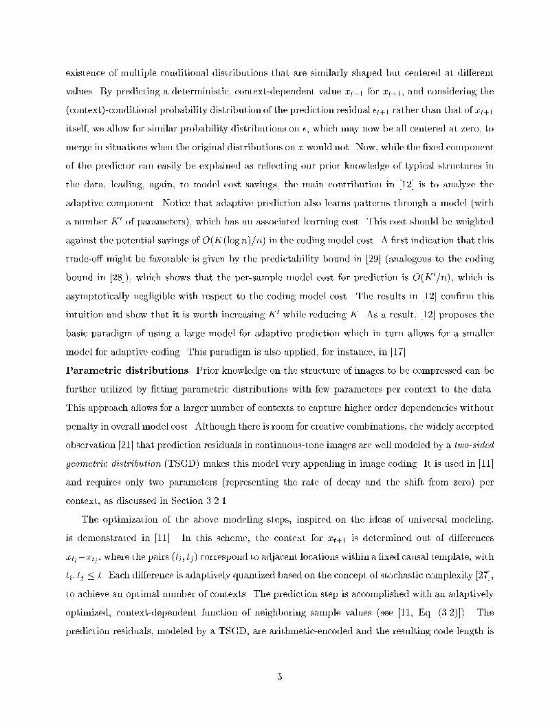
Summary. The overall simplicity of LOCO-I/JPEG-LS can be mainly attributed to its success

in matching the complexity of the modeling and coding units, combining simplicity with the com-

pression potential of context models, thus \enjoying the best of both worlds." The main blocks

of the algorithm are depicted in Figure 1, including the causal template actually employed. The

shaded area in the image icon at the left of the �gure represents the scanned past data xt, on which

2A speci�c linear predicting function is demonstrated in [11], as an example of the general setting. However,

all implementations of the algorithm also include an a�ne term, which is estimated through the average of past

prediction errors, as suggested in [11, p. 583].3The use of Golomb codes in conjunction with context modeling was pioneered in the FELICS algorithm [24].

6

FixedPredictor

AdaptiveCorrectionFlat

Region?

Gradients

ContextModeler

RunCounter

RunCoder

Modeler Coder

GolombCoder

imagesamples

imagesamples

context

imagesamples

compressedbitstream

predictedvalues

predictionerrors

Predictor

pred. errors,code spec.

run lengths,code spec.

regular regular

run runmode mode

c

a

b d

x

Figure 1: JPEG-LS: Block Diagram

prediction and context modeling are based, while the black dot represents the sample xt+1 currently

encoded. The switches labeled mode select operation in \regular" or \run" mode, as determined

from xt by a simple region \ atness" criterion.

3 Detailed description of JPEG-LS

The prediction and modeling units in JPEG-LS are based on the causal template depicted in

Figure 1, where x denotes the current sample, and a; b; c, and d, are neighboring samples in the

relative positions shown in the �gure.4 The dependence of a; b; c; d, and x, on the time index

t has been deleted from the notation for simplicity. Moreover, by abuse of notation, we will use

a; b; c; d, and x to denote both the values of the samples and their locations. By using the template

of Figure 1, JPEG-LS limits its image bu�ering requirement to one scan line.

3.1 Prediction

Ideally, the value guessed for the current sample x should depend on a; b; c, and d through an

adaptive model of the local edge direction. While our complexity constraints rule out this possibility,

some form of edge detection is still desirable. In LOCO-I/JPEG-LS, a �xed predictor performs a

primitive test to detect vertical or horizontal edges, while the adaptive part is limited to an integer

additive term, which is context-dependent as in [11] and re ects the a�ne term in classical AR

models (e.g., [31]). Speci�cally, the �xed predictor in LOCO-I/JPEG-LS guesses:

x̂MED�=

8><>:

min(a; b) if c � max(a; b)

max(a; b) if c � min(a; b)

a+ b� c otherwise.

(1)

4The causal template in [1] includes an additional sample, e, West of a. This location was discarded in the course

of the standardization process as its contribution was not deemed to justify the additional context storage required [4].

7

The predictor (1) switches between three simple predictors: it tends to pick b in cases where a

vertical edge exists left of the current location, a in cases of an horizontal edge above the current

location, or a + b � c if no edge is detected. The latter choice would be the value of x if the

current sample belonged to the \plane" de�ned by the three neighboring samples with \heights"

a, b, and c. This expresses the expected smoothness of the image in the absence of edges. The

predictor (1) has been used in image compression applications [37], under a di�erent interpretation:

The guessed value is seen as the median of three �xed predictors, a; b, and a + b � c. Combining

both interpretations, this predictor was renamed during the standardization process \median edge

detector" (MED).

As for the integer adaptive term, it e�ects a context-dependent translation. Therefore, it can

be interpreted as part of the estimation procedure for the TSGD. This procedure is discussed in

Section 3.2. Notice that d is employed in the adaptive part of the predictor, but not in (1).

3.2 Context Modeling

As noted in Section 2.1, reducing the number of parameters is a key objective in a context mod-

eling scheme. This number is determined by the number of free parameters de�ning the coding

distribution at each context and by the number of contexts.

3.2.1 Parameterization

The TSGD model. It is a widely accepted observation [21] that the global statistics of residuals

from a �xed predictor in continuous-tone images are well-modeled by a TSGD centered at zero.

According to this distribution, the probability of an integer value � of the prediction error is

proportional to �j�j, where � 2 (0; 1) controls the two-sided exponential decay rate. However, it was

observed in [15] that a DC o�set is typically present in context-conditioned prediction error signals.

This o�set is due to integer-value constraints and possible bias in the prediction step. Thus, a more

general model, which includes an additional o�set parameter �, is appropriate. Letting � take non-

integer values, the two adjacent modes often observed in empirical context-dependent histograms

of prediction errors are also better captured by this model. We break the �xed prediction o�set

into an integer part R (or \bias"), and a fractional part s (or \shift"), such that � = R � s,

where 0 � s < 1. Thus, the TSGD parametric class P(�;�), assumed by LOCO-I/JPEG-LS for the

residuals of the �xed predictor at each context, is given by

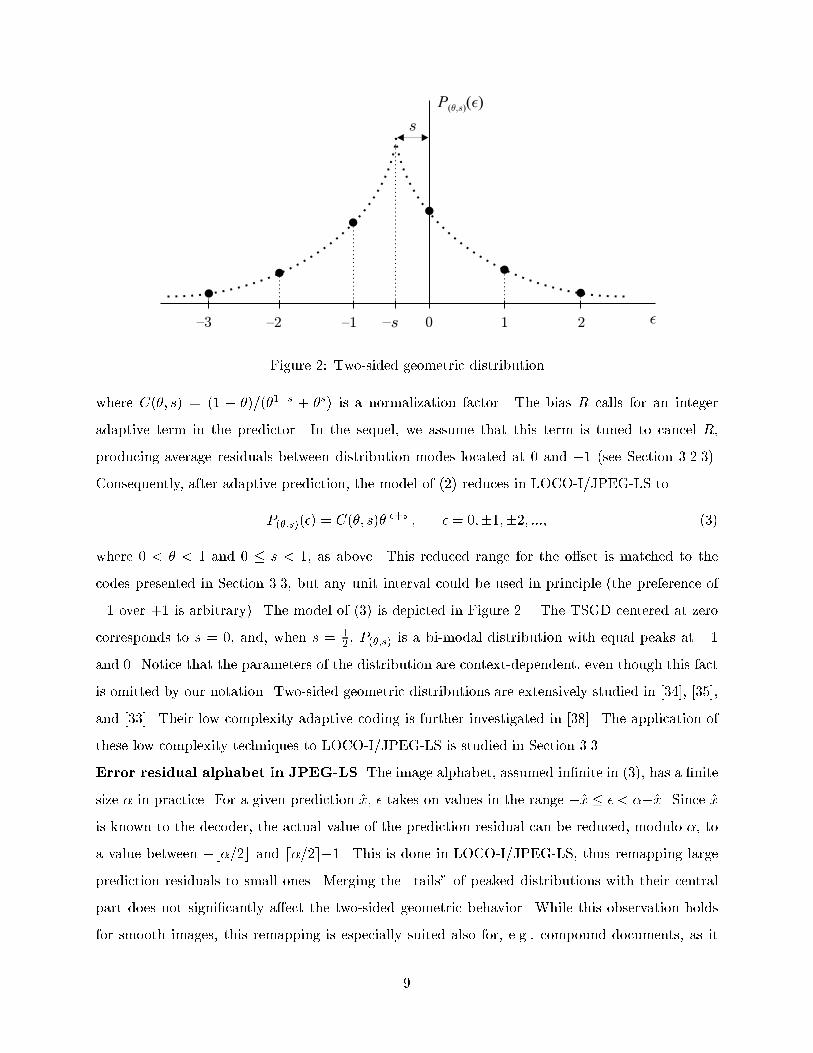
P(�;�)(�) = C(�; s)�j��R+sj; � = 0;�1;�2; :::; (2)

8

{3 {2 {1 0 1 2

s

{s

P( )µ;s ( )²

²

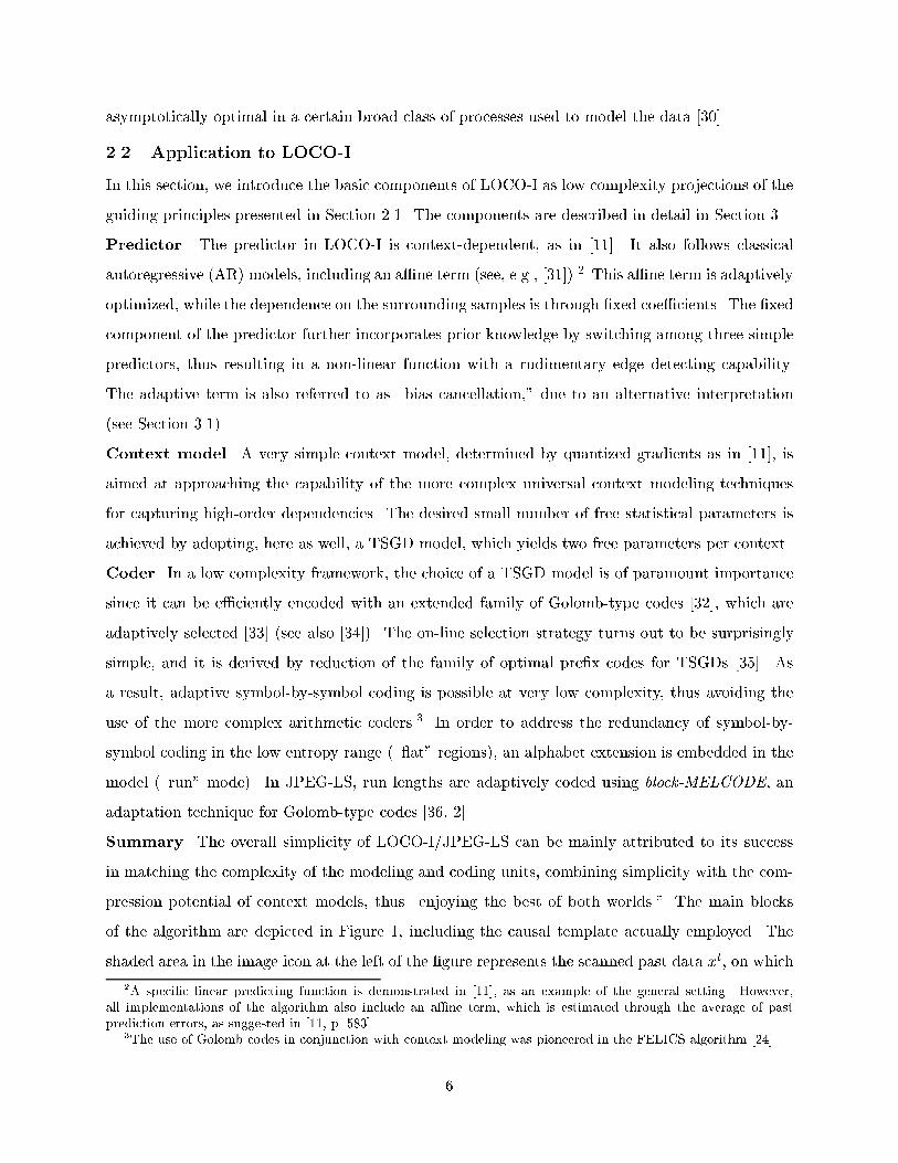
Figure 2: Two-sided geometric distribution

where C(�; s) = (1 � �)=(�1�s + �s) is a normalization factor. The bias R calls for an integer

adaptive term in the predictor. In the sequel, we assume that this term is tuned to cancel R,

producing average residuals between distribution modes located at 0 and �1 (see Section 3.2.3).

Consequently, after adaptive prediction, the model of (2) reduces in LOCO-I/JPEG-LS to

P(�;s)(�) = C(�; s)�j�+sj; � = 0;�1;�2; :::; (3)

where 0 < � < 1 and 0 � s < 1, as above. This reduced range for the o�set is matched to the

codes presented in Section 3.3, but any unit interval could be used in principle (the preference of

�1 over +1 is arbitrary). The model of (3) is depicted in Figure 2. The TSGD centered at zero

corresponds to s = 0, and, when s = 12, P(�;s) is a bi-modal distribution with equal peaks at �1

and 0. Notice that the parameters of the distribution are context-dependent, even though this fact

is omitted by our notation. Two-sided geometric distributions are extensively studied in [34], [35],

and [33]. Their low complexity adaptive coding is further investigated in [38]. The application of

these low complexity techniques to LOCO-I/JPEG-LS is studied in Section 3.3.

Error residual alphabet in JPEG-LS. The image alphabet, assumed in�nite in (3), has a �nite

size � in practice. For a given prediction x̂, � takes on values in the range �x̂ � � < ��x̂. Since x̂

is known to the decoder, the actual value of the prediction residual can be reduced, modulo �, to

a value between �b�=2c and d�=2e�1. This is done in LOCO-I/JPEG-LS, thus remapping large

prediction residuals to small ones. Merging the \tails" of peaked distributions with their central

part does not signi�cantly a�ect the two-sided geometric behavior. While this observation holds

for smooth images, this remapping is especially suited also for, e.g., compound documents, as it

9

assigns a large probability to sharp transitions. In the common case � = 2� , it consists of just

interpreting the � least signi�cant bits of � in 2's complement representation.5 Since � is typically

quite large, we will continue to use the in�nite alphabet model (3), although the reduced prediction

residuals, still denoted by �, belong to the �nite range [�b�=2c; d�=2e�1].

3.2.2 Context determination

General approach. The context that conditions the encoding of the current prediction residual

in JPEG-LS is built out of the di�erences g1 = d� b; g2 = b� c, and g3 = c� a. These di�erences

represent the local gradient, thus capturing the level of activity (smoothness, edginess) surrounding

a sample, which governs the statistical behavior of prediction errors. Notice that this approach

di�ers from the one adopted in the Sunset family [16] and other schemes, where the context is

built out of the prediction errors incurred in previous encodings. By symmetry,6 g1; g2, and g3

in uence the model in the same way. Since further model size reduction is obviously needed, each

di�erence gj ; j = 1; 2; 3, is quantized into a small number of approximately equiprobable, connected

regions by a quantizer �(�) independent of j. In a well-de�ned theoretical setting, this maximizes

the mutual information between the current sample value and its context, an information-theoretic

measure of the amount of information provided by the conditioning context on the sample value to

be modeled. We refer to [11] and [12] for an in depth theoretical discussion of these issues.

In principle, the number of regions into which each context di�erence is quantized should

be adaptively optimized. However, the low complexity requirement dictates a �xed number of

\equiprobable" regions. To preserve symmetry, the regions are indexed �T; � � � ;�1; 0; 1; � � � ; T ,

with �(g) = ��(�g), for a total of (2T +1)3 di�erent contexts. A further reduction in the number

of contexts is obtained after observing that, by symmetry, it is reasonable to assume that

Probf�t+1 = � jCt = [q1; q2; q3]g = Probf�t+1 = �� jCt = [�q1; �q2; �q3]g

where Ct represents the quantized context triplet and qj = �(gj); j=1; 2; 3. Hence, if the �rst non-

zero element of Ct is negative, the encoded value is ��t+1, using context �Ct. This is anticipated

by the decoder, which ips the error sign if necessary to obtain the original error value. By merging

contexts of \opposite signs," the total number of contexts becomes ((2T + 1)3 + 1)=2.

Contexts in JPEG-LS. For JPEG-LS, T = 4 was selected, resulting in 365 contexts. This number

balances storage requirements (which are roughly proportional to the number of contexts) with

5A higher complexity remapping is discussed in [39].6Here, we assume that the class of images to be encoded is essentially symmetric with respect to horizontal/vertical,

left/right, and top/bottom transpositions, as well as the sample value \negation" transformation x! (��1�x).

10

high-order conditioning. In fact, due to the parametric model of equation (3), more contexts could

be a�orded for medium-sized to large images, without incurring an excessive model cost. However,

the compression improvement is marginal and does not justify the increase in resources [4]. For

small images, it is possible to reduce the number of contexts within the framework of the standard,

as discussed below.

To complete the de�nition of the contexts in JPEG-LS, it remains to specify the boundaries

between quantization regions. For an 8-bit/sample alphabet, the default quantization regions are

f0g, �f1; 2g, �f3; 4; 5; 6g, �f7; 8; � � � ; 20g, �f e j e � 21 g. However, the boundaries are adjustable

parameters, except that the central region must be f0g. In particular, a suitable choice collapses

quantization regions, resulting in a smaller e�ective number of contexts, with applications to the

compression of small images. For example, a model with 63 contexts (T = 2), was found to work

best for the 64� 64-tile size used in the FlashPixTM �le format [40]. Through appropriate scaling,

default boundary values are also provided for general alphabet sizes � [3, 7].

3.2.3 Adaptive correction

As mentioned in sections 3.1 and 3.2.1, the adaptive part of the predictor is context-based and it

is used to \cancel" the integer part R of the o�set due to the �xed predictor. As a result, the

context-dependent shift in the distributions (3) was restricted to the range 0 � s < 1. This section

discusses how this adaptive correction (or bias cancellation) is performed at low complexity.

Bias estimation. In principle, maximum-likelihood (ML) estimation of R in (2) would dictate

a bias cancellation procedure based on the median of the prediction errors incurred so far in the

context by the �xed predictor (1). However, storage constraints rule out this possibility. Instead, an

estimate based on the average could be obtained by just keeping a count N of context occurrences,

and a cumulative sum D of �xed prediction errors incurred so far in the context. Then, a correction

value C 0 could be computed as the rounded average

C 0 = dD=Ne (4)

and added to the �xed prediction x̂MED, to o�set the prediction bias. This approach, however,

has two main problems. First, it requires a general division, in opposition to the low complexity

requirements of LOCO-I/JPEG-LS. Second, it is very sensitive to the in uence of \outliers," i.e.,

atypical large errors can a�ect future values of C 0 until it returns to its typical value, which is quite

stable.

11

To solve these problems, �rst notice that (4) is equivalent to

D = N � C 0 +B0 ;

where the integer B0 satis�es �N < B0 � 0. It is readily veri�ed, by setting up a simple recur-

sion, that the correction value can be implemented by storing B0 and C 0, and adjusting both for

each occurrence of the context. The corrected prediction error � is �rst added to B0, and then N

is subtracted or added until the result is in the desired range (�N; 0]. The number of subtrac-

tions/additions of N prescribes the adjustment for C 0.

Bias computation in JPEG-LS. The above procedure is further modi�ed in LOCO-I/JPEG-LS

by limiting the number of subtractions/additions to one per update, and then \forcing" the value

of B0 into the desired range, if needed. Speci�cally, C 0 and B0 are replaced by approximate values

C and B, respectively, which are initialized to zero and updated according to the division-free

procedure shown in Figure 3 (in C-language style). The procedure increments (resp. decrements)

B = B + �; /* accumulate prediction residual */

N = N + 1; /* update occurrence counter */

/* update correction value and shift statistics */

if ( B � �N ) fC = C � 1; B = B +N ;

if ( B � �N ) B = �N + 1;

gelse if ( B > 0 ) f

C = C + 1; B = B �N ;

if ( B > 0 ) B = 0;

gFigure 3: Bias computation procedure

the correction value C each time B > 0 (resp. B � �N). At this time, B is also adjusted to re ect

the change in C. If the increment (resp. decrement) is not enough to bring B to the desired range

(i.e., the adjustment in C was limited), B is clamped to 0 (resp. �N + 1). This procedure will

tend to produce average prediction residuals in the interval (�1; 0], with C serving as an estimate

(albeit not the ML one) of R. Notice that �B=N is an estimate of the residual fractional shift

parameter s (again, not the ML one). To reduce storage requirements, C is not incremented (resp.

decremented) over 127 (resp. under �128). Mechanisms for \centering" image prediction error

distributions, based on integer o�set models, are described in [15] and [17].

12

3.3 Coding

To encode corrected prediction residuals distributed according to the TSGD of (3), LOCO-I/JPEG-

LS uses a minimal complexity sub-family of the family of optimal pre�x codes for TSGDs, recently

characterized in [35]. The coding unit also implements a low complexity adaptive strategy to

sequentially select a code among the above sub-family. In this sub-section, we discuss the codes

of [35] and the principles guiding general adaptation strategies, and show how the codes and the

principles are simpli�ed to yield the adopted solution.

3.3.1 Golomb codes and optimal pre�x codes for the TSGD

The optimal codes of [35] are based on Golomb codes [32], whose structure enables simple calculation

of the code word of any given sample, without recourse to the storage of code tables, as would be

the case with unstructured, generic Hu�man codes. In an adaptive mode, a structured family of

codes further relaxes the need of dynamically updating code tables due to possible variations in

the estimated parameters (see, e.g., [41]).

Golomb codes were �rst described in [32], as a means for encoding run lengths. Given a positive

integer parameter m, the mth order Golomb code Gm encodes an integer y � 0 in two parts: a

unary representation of by=mc, and a modi�ed binary representation of ymodm (using blogmc

bits if y < 2dlogme�m and dlogme bits otherwise). Golomb codes are optimal [42] for one-sided

geometric distributions (OSGDs) of the nonnegative integers, i.e., distributions of the form (1��)�y,

where 0 < � < 1. Thus, for every � there exists a value of m such that Gm yields the shortest

average code length over all uniquely decipherable codes for the nonnegative integers.

The special case of Golomb codes with m = 2k leads to very simple encoding/decoding pro-

cedures: the code for y is constructed by appending the k least signi�cant bits of y to the unary

representation of the number formed by the remaining higher order bits of y (the simplicity of the

case m = 2k was already noted in [32]). The length of the encoding is k + 1 + by=2kc. We refer to

codes G2k as Golomb-power-of-2 (GPO2) codes.

In the characterization of optimal pre�x codes for TSGDs in [35], the parameter space (�; s)

is partitioned into regions, and a di�erent optimal pre�x code corresponds to each region (s � 12

is assumed, since the case s > 12can be reduced to the former by means of the re ection/shift

transformation � ! �(� + 1) on the TSG-distributed variable �). Each region is associated with

an m-th order Golomb code, where the parameter m is a function of the values of � and s in the

region. Depending on the region, an optimal code from [35] encodes an integer � either by applying

13

a region-dependent modi�cation of Gm to j�j, followed by a sign bit whenever � 6= 0, or by using

Gm(M(�)), where

M(�) = 2j�j � u(�) ; (5)

and the indicator function u(�) = 1 if � < 0, or 0 otherwise. Codes of the �rst type are not

used in LOCO-I/JPEG-LS, and are not discussed further in this paper. Instead, we focus on

the mapping M(�), which gives the index of � in the interleaved sequence 0;�1; 1;�2; 2; : : : This

mapping was �rst used by Rice in [39] to encode TSGDs centered at zero, by applying a GPO2 code

to M(�). Notice that M(�) is a very natural mapping under the assumption s � 12, since it sorts

prediction residuals in non-increasing order of probability. The corresponding mapping for s > 12

is M 0(�) = M(���1), which e�ects the probability sorting in this case. Following the modular

reduction described in Section 3.2.1, for �b�=2c � � � d�=2e�1, the corresponding values M(�)

fall in the range 0 �M(�) � ��1. This is also the range for M 0(�) with even �. For odd �, M 0(�)

can also take on the value � (but not ��1).

3.3.2 Sequential parameter estimation

Statement of the problem. Even though, in general, adaptive strategies are easier to imple-

ment with arithmetic codes, the family of codes of [35] provides a reasonable alternative for low

complexity adaptive coding of TSGDs, which is investigated in [33]: Based on the past sequence

of prediction residuals �t = �1�2 � � � �t encoded at a given context, select a code (i.e., an optimal-

ity region, which includes a Golomb parameter m) sequentially, and use this code to encode �t+1.

(Notice that t here indexes occurrences of a given context, thus corresponding to the variable N

introduced in Section 3.2.3.) The decoder makes the same determination, after decoding the same

past sequence. Thus, the coding is done \on the y," as with adaptive arithmetic coders. Two

adaptation approaches are possible for selecting the code for �t+1: exhaustive search of the code

that would have performed best on �t, or expected code length minimization for an estimate of the

TSGD parameters given �t. These two approaches also apply in a block coding framework,7 with

the samples in the block to be encoded used in lieu of �t.

An advantage of the estimation approach is that, if based on ML, it depends only on the

su�cient statistics St and Nt for the parameters � and s, given by

St =tX

i=1

(j�ij � u(�i)) ; Nt =tX

i=1

u(�i) ;

7For block coding, an image is divided into rectangular blocks of samples. The blocks are scanned to select a code

within a small family, which is identi�ed with a few overhead bits, and the samples are encoded in a second pass

through the block (see, e.g., [39]).

14

with u(�) as in (5). Clearly, Nt is the total number of negative samples in �t, and St + Nt is the

accumulated sum of absolute values. In contrast, an exhaustive search would require one counter

per context for each code in the family.

Code family reduction. Despite the relative simplicity of the codes, the complexity of both the

code determination and the encoding procedure for the full family of optimal codes of [35] would still

be beyond the constraints set for JPEG-LS. For that reason, as in [39], LOCO-I/JPEG-LS only

uses the sub-family of GPO2 codes. Furthermore, only codes based on the mappings M(�) and

M 0(�) (for s � 12and s > 1

2, respectively) are used. We denote �k(�) = G2k(M(�)). The mapping

M 0(�) is relevant only for k = 0, since �k(�) = �k(���1) for every k > 0. Thus, the sequential code

selection process in LOCO-I/JPEG-LS consists of the selection of a Golomb parameter k,8 and in

case k = 0, a mapping M(�) or M 0(�). We further denote �00(�) = G1(M0(�)).

The above sub-family of codes, which we denote C, represents a speci�c compression-complexity

trade-o�. It is shown in [35] that the average code length with the best code in C is within about

4:7% of the optimal pre�x codes for TSGDs, with largest deterioration in the very low entropy

region, where a di�erent coding method is needed anyway (see Section 3.5). Furthermore, it is

shown in [38] that the gap is reduced to about 1:8% by including codes based on one of the other

mappings mentioned above, with a slightly more complex adaptation strategy. These results are

consistent with estimates in [39] for the redundancy of GPO2 codes on OSGDs.

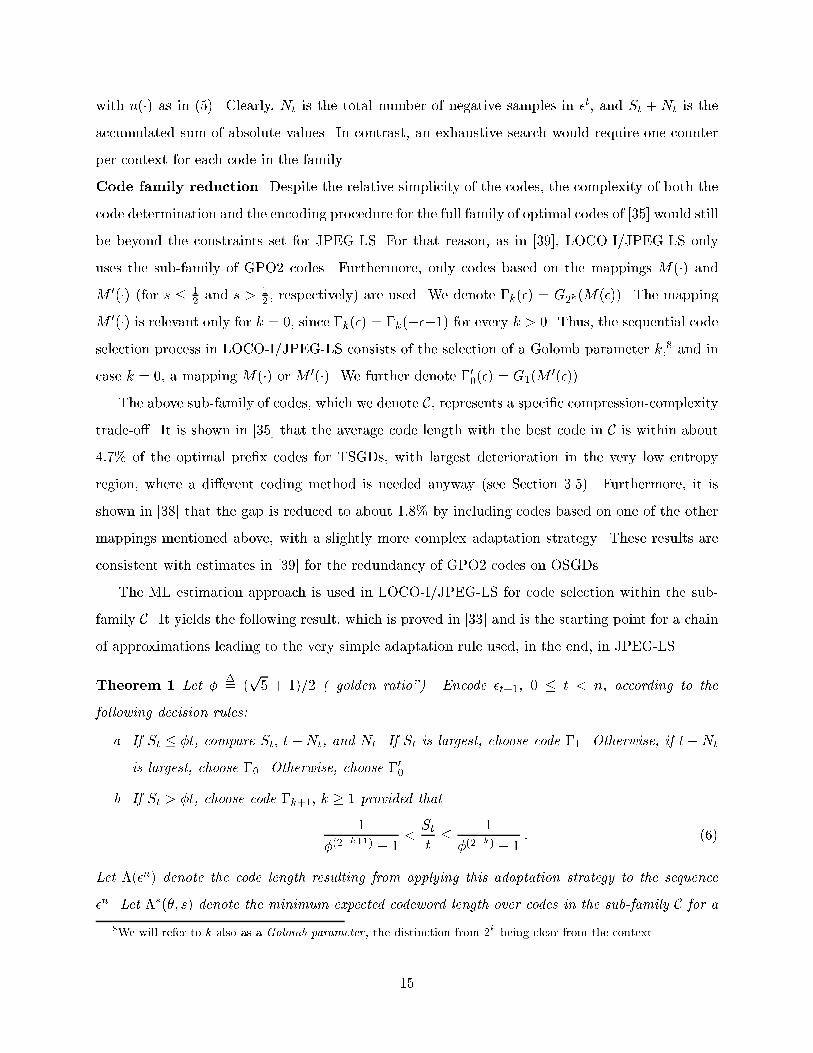
The ML estimation approach is used in LOCO-I/JPEG-LS for code selection within the sub-

family C. It yields the following result, which is proved in [33] and is the starting point for a chain

of approximations leading to the very simple adaptation rule used, in the end, in JPEG-LS.

Theorem 1 Let ��= (

p5 + 1)=2 (\golden ratio"). Encode �t+1, 0 � t < n, according to the

following decision rules:

a. If St � �t, compare St; t�Nt, and Nt. If St is largest, choose code �1. Otherwise, if t�Nt

is largest, choose �0. Otherwise, choose �00.

b. If St > �t, choose code �k+1; k � 1 provided that

1

�(2�k+1) � 1

<St

t�

1

�(2�k) � 1

: (6)

Let �(�n) denote the code length resulting from applying this adaptation strategy to the sequence

�n. Let ��(�; s) denote the minimum expected codeword length over codes in the sub-family C for a

8We will refer to k also as a Golomb parameter , the distinction from 2k being clear from the context.

15

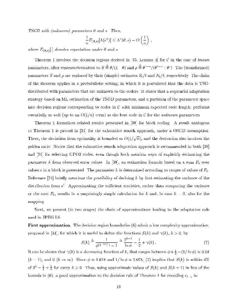
TSGD with (unknown) parameters � and s. Then,

1

nE(�;s)[�(�

n)] � ��(�; s) +O

�1

n

�;

where E(�;s)[�] denotes expectation under � and s.

Theorem 1 involves the decision regions derived in [35, Lemma 4] for C in the case of known

parameters, after reparameterization to S�= �=(1��) and �

�= �1�s=(�1�s+�s). The (transformed)

parameters S and � are replaced by their (simple) estimates St=t and Nt=t, respectively. The claim

of the theorem applies in a probabilistic setting, in which it is postulated that the data is TSG-

distributed with parameters that are unknown to the coders. It states that a sequential adaptation

strategy based on ML estimation of the TSGD parameters, and a partition of the parameter space

into decision regions corresponding to codes in C with minimum expected code length, performs

essentially as well (up to an O(1=n) term) as the best code in C for the unknown parameters.

Theorem 1 formalizes related results presented in [39] for block coding. A result analogous

to Theorem 1 is proved in [24] for the exhaustive search approach, under a OSGD assumption.

There, the deviation from optimality is bounded as O(1=pn), and the derivation also involves the

golden ratio. Notice that the exhaustive search adaptation approach is recommended in both [39]

and [24] for selecting GPO2 codes, even though both mention ways of explicitly estimating the

parameter k from observed error values. In [39], an estimation formula based on a sum F0 over

values � in a block is presented. The parameter k is determined according to ranges of values of F0.

Reference [24] brie y mentions the possibility of deriving k by �rst estimating the variance of the

distribution from �t. Approximating the su�cient statistics, rather than computing the variance

or the sum F0, results in a surprisingly simple calculation for k and, in case k = 0, also for the

mapping.

Next, we present (in two stages) the chain of approximations leading to the adaptation rule

used in JPEG-LS.

First approximation. The decision region boundaries (6) admit a low complexity approximation,

proposed in [33], for which it is useful to de�ne the functions S(k) and (k), k > 0, by

S(k)�=

1

�(2�k+1) � 1

�=

2k�1

ln��1

2+ (k) : (7)

It can be shown that (k) is a decreasing function of k, that ranges between �+ 12� (1= ln�) � 0:04

(k = 1), and 0 (k ! 1). Since � � 1:618 and 1= ln� � 2:078, (7) implies that S(k) is within 4%

of 2k � 12+ 1

8for every k > 0. Thus, using approximate values of S(k) and S(k + 1) in lieu of the

bounds in (6), a good approximation to the decision rule of Theorem 1 for encoding �t+1 is:

16

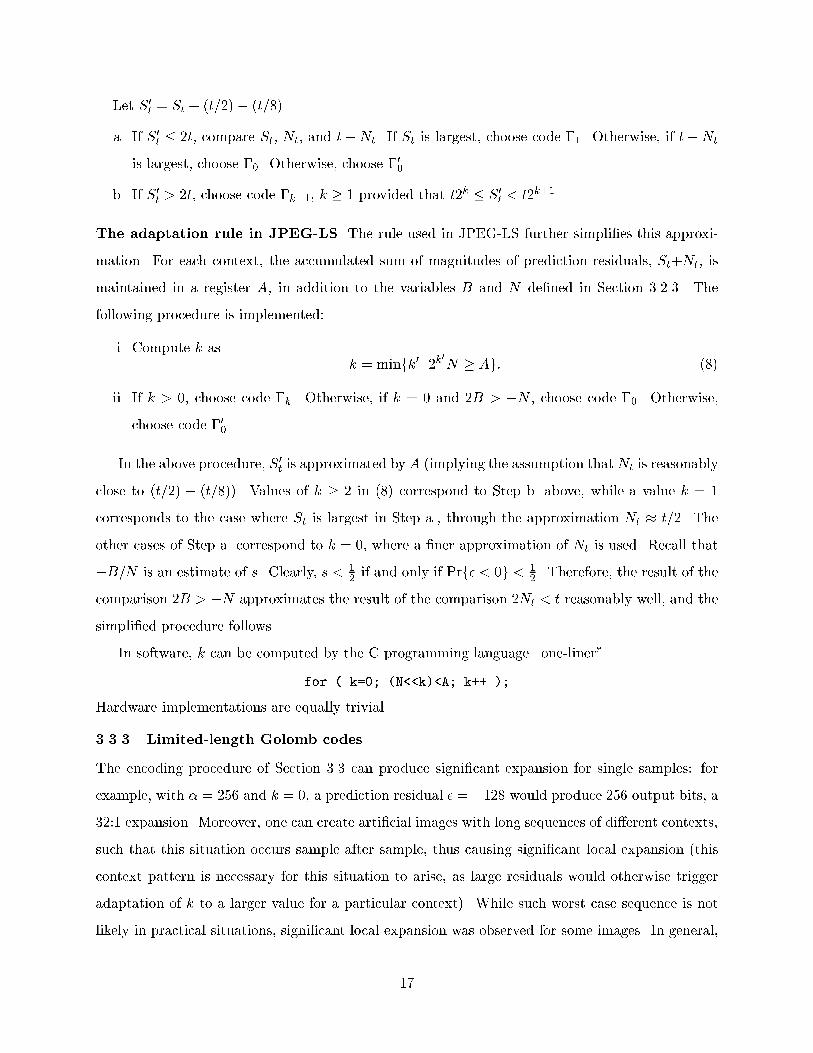
Let S0t = St + (t=2) � (t=8).

a. If S0t � 2t, compare St; Nt, and t�Nt. If St is largest, choose code �1. Otherwise, if t�Nt

is largest, choose �0. Otherwise, choose �00.

b. If S0t > 2t, choose code �k+1; k � 1 provided that t2k � S0

t < t2k+1.

The adaptation rule in JPEG-LS. The rule used in JPEG-LS further simpli�es this approxi-

mation. For each context, the accumulated sum of magnitudes of prediction residuals, St+Nt, is

maintained in a register A, in addition to the variables B and N de�ned in Section 3.2.3. The

following procedure is implemented:

i. Compute k ask = minfk0 j 2k

0

N � Ag: (8)

ii. If k > 0, choose code �k. Otherwise, if k = 0 and 2B > �N , choose code �0. Otherwise,

choose code �00.

In the above procedure, S0t is approximated by A (implying the assumption that Nt is reasonably

close to (t=2) � (t=8)). Values of k � 2 in (8) correspond to Step b. above, while a value k = 1

corresponds to the case where St is largest in Step a., through the approximation Nt � t=2. The

other cases of Step a. correspond to k = 0, where a �ner approximation of Nt is used. Recall that

�B=N is an estimate of s. Clearly, s < 12if and only if Prf� < 0g < 1

2. Therefore, the result of the

comparison 2B > �N approximates the result of the comparison 2Nt < t reasonably well, and the

simpli�ed procedure follows.

In software, k can be computed by the C programming language \one-liner"

for ( k=0; (N<<k)<A; k++ );

Hardware implementations are equally trivial.

3.3.3 Limited-length Golomb codes

The encoding procedure of Section 3.3 can produce signi�cant expansion for single samples: for

example, with � = 256 and k = 0, a prediction residual � = �128 would produce 256 output bits, a

32:1 expansion. Moreover, one can create arti�cial images with long sequences of di�erent contexts,

such that this situation occurs sample after sample, thus causing signi�cant local expansion (this

context pattern is necessary for this situation to arise, as large residuals would otherwise trigger

adaptation of k to a larger value for a particular context). While such worst case sequence is not

likely in practical situations, signi�cant local expansion was observed for some images. In general,

17

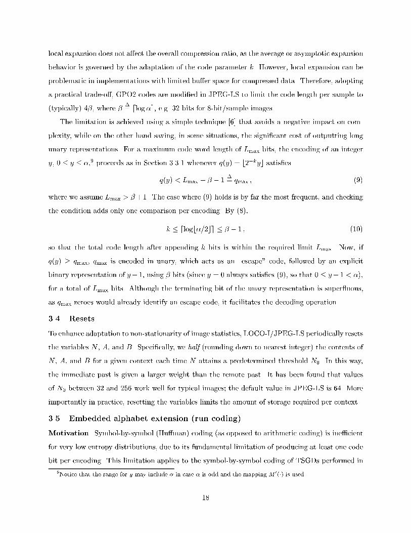
local expansion does not a�ect the overall compression ratio, as the average or asymptotic expansion

behavior is governed by the adaptation of the code parameter k. However, local expansion can be

problematic in implementations with limited bu�er space for compressed data. Therefore, adopting

a practical trade-o�, GPO2 codes are modi�ed in JPEG-LS to limit the code length per sample to

(typically) 4�, where ��= dlog�e, e.g. 32 bits for 8-bit/sample images.

The limitation is achieved using a simple technique [6] that avoids a negative impact on com-

plexity, while on the other hand saving, in some situations, the signi�cant cost of outputting long

unary representations. For a maximum code word length of Lmax bits, the encoding of an integer

y; 0 � y � �,9 proceeds as in Section 3.3.1 whenever q(y) = b2�kyc satis�es

q(y) < Lmax � � � 1�= qmax ; (9)

where we assume Lmax > �+1. The case where (9) holds is by far the most frequent, and checking

the condition adds only one comparison per encoding. By (8),

k � dlogb�=2ce � � � 1 ; (10)

so that the total code length after appending k bits is within the required limit Lmax. Now, if

q(y) � qmax, qmax is encoded in unary, which acts as an \escape" code, followed by an explicit

binary representation of y� 1, using � bits (since y = 0 always satis�es (9), so that 0 � y� 1 < �),

for a total of Lmax bits. Although the terminating bit of the unary representation is super uous,

as qmax zeroes would already identify an escape code, it facilitates the decoding operation.

3.4 Resets

To enhance adaptation to non-stationarity of image statistics, LOCO-I/JPEG-LS periodically resets

the variables N , A, and B. Speci�cally, we half (rounding down to nearest integer) the contents of

N , A, and B for a given context each time N attains a predetermined threshold N0. In this way,

the immediate past is given a larger weight than the remote past. It has been found that values

of N0 between 32 and 256 work well for typical images; the default value in JPEG-LS is 64. More

importantly in practice, resetting the variables limits the amount of storage required per context.

3.5 Embedded alphabet extension (run coding)

Motivation. Symbol-by-symbol (Hu�man) coding (as opposed to arithmetic coding) is ine�cient

for very low entropy distributions, due to its fundamental limitation of producing at least one code

bit per encoding. This limitation applies to the symbol-by-symbol coding of TSGDs performed in

9Notice that the range for y may include � in case � is odd and the mapping M0(�) is used.

18

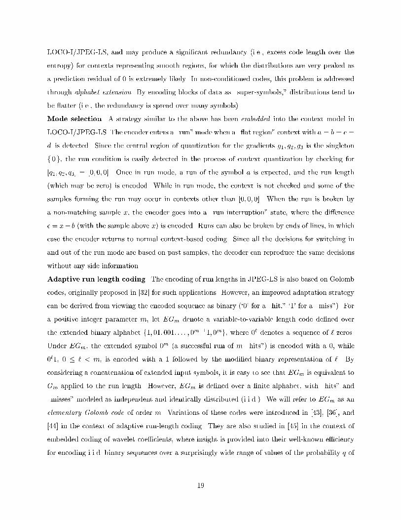
LOCO-I/JPEG-LS, and may produce a signi�cant redundancy (i.e., excess code length over the

entropy) for contexts representing smooth regions, for which the distributions are very peaked as

a prediction residual of 0 is extremely likely. In non-conditioned codes, this problem is addressed

through alphabet extension. By encoding blocks of data as \super-symbols," distributions tend to

be atter (i.e., the redundancy is spread over many symbols).

Mode selection. A strategy similar to the above has been embedded into the context model in

LOCO-I/JPEG-LS. The encoder enters a \run" mode when a \ at region" context with a = b = c =

d is detected. Since the central region of quantization for the gradients g1; g2; g3 is the singleton

f 0 g, the run condition is easily detected in the process of context quantization by checking for

[q1; q2; q3] = [0; 0; 0]. Once in run mode, a run of the symbol a is expected, and the run length

(which may be zero) is encoded. While in run mode, the context is not checked and some of the

samples forming the run may occur in contexts other than [0; 0; 0]. When the run is broken by

a non-matching sample x, the encoder goes into a \run interruption" state, where the di�erence

� = x� b (with the sample above x) is encoded. Runs can also be broken by ends of lines, in which

case the encoder returns to normal context-based coding. Since all the decisions for switching in

and out of the run mode are based on past samples, the decoder can reproduce the same decisions

without any side information.

Adaptive run length coding. The encoding of run lengths in JPEG-LS is also based on Golomb

codes, originally proposed in [32] for such applications. However, an improved adaptation strategy

can be derived from viewing the encoded sequence as binary (`0' for a \hit," `1' for a \miss"). For

a positive integer parameter m, let EGm denote a variable-to-variable length code de�ned over

the extended binary alphabet f1; 01; 001; : : : ; 0m�11; 0mg, where 0` denotes a sequence of ` zeros.

Under EGm, the extended symbol 0m (a successful run of m \hits") is encoded with a 0, while

0`1, 0 � ` < m, is encoded with a 1 followed by the modi�ed binary representation of `. By

considering a concatenation of extended input symbols, it is easy to see that EGm is equivalent to

Gm applied to the run length. However, EGm is de�ned over a �nite alphabet, with \hits" and

\misses" modeled as independent and identically distributed (i.i.d.). We will refer to EGm as an

elementary Golomb code of order m. Variations of these codes were introduced in [43], [36], and

[44] in the context of adaptive run-length coding. They are also studied in [45] in the context of

embedded coding of wavelet coe�cients, where insight is provided into their well-known e�ciency

for encoding i.i.d. binary sequences over a surprisingly wide range of values of the probability q of

19

a zero.

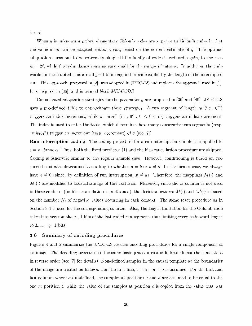
When q is unknown a priori , elementary Golomb codes are superior to Golomb codes in that

the value of m can be adapted within a run, based on the current estimate of q. The optimal

adaptation turns out to be extremely simple if the family of codes is reduced, again, to the case

m = 2g, while the redundancy remains very small for the ranges of interest. In addition, the code

words for interrupted runs are all g+1 bits long and provide explicitly the length of the interrupted

run. This approach, proposed in [2], was adopted in JPEG-LS and replaces the approach used in [1].

It is inspired in [36], and is termed block-MELCODE .

Count-based adaptation strategies for the parameter g are proposed in [36] and [45]. JPEG-LS

uses a pre-de�ned table to approximate these strategies. A run segment of length m (i.e., 0m)

triggers an index increment, while a \miss" (i.e., 0`1, 0 � ` < m) triggers an index decrement.

The index is used to enter the table, which determines how many consecutive run segments (resp.

\misses") trigger an increment (resp. decrement) of g (see [7]).

Run interruption coding. The coding procedure for a run interruption sample x is applied to

� = x�bmod�. Thus, both the �xed predictor (1) and the bias cancellation procedure are skipped.

Coding is otherwise similar to the regular sample case. However, conditioning is based on two

special contexts, determined according to whether a = b or a 6= b. In the former case, we always

have � 6= 0 (since, by de�nition of run interruption, x 6= a). Therefore, the mappings M(�) and

M 0(�) are modi�ed to take advantage of this exclusion. Moreover, since the B counter is not used

in these contexts (no bias cancellation is performed), the decision between M(�) and M 0(�) is based

on the number Nt of negative values occurring in each context. The same reset procedure as in

Section 3.4 is used for the corresponding counters. Also, the length limitation for the Golomb code

takes into account the g+1 bits of the last coded run segment, thus limiting every code word length

to Lmax�g�1 bits.

3.6 Summary of encoding procedures

Figures 4 and 5 summarize the JPEG-LS lossless encoding procedures for a single component of

an image. The decoding process uses the same basic procedures and follows almost the same steps

in reverse order (see [7] for details). Non-de�ned samples in the causal template at the boundaries

of the image are treated as follows: For the �rst line, b = c = d = 0 is assumed. For the �rst and

last column, whenever unde�ned, the samples at positions a and d are assumed to be equal to the

one at position b, while the value of the samples at position c is copied from the value that was

20

assigned to position a when encoding the �rst sample in the previous line.

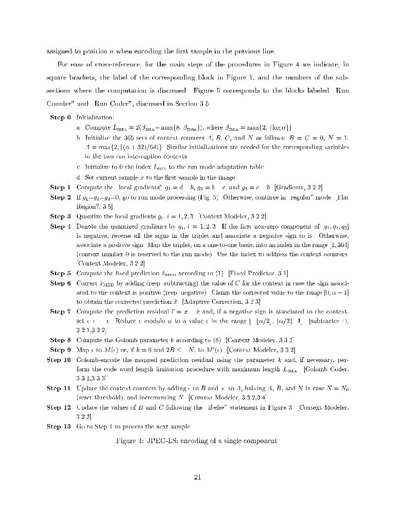
For ease of cross-reference, for the main steps of the procedures in Figure 4 we indicate, in

square brackets, the label of the corresponding block in Figure 1, and the numbers of the sub-

sections where the computation is discussed. Figure 5 corresponds to the blocks labeled \Run

Counter" and \Run Coder", discussed in Section 3.5.

Step 0. Initialization:

a. Compute Lmax = 2(�max+maxf8; �maxg), where �max = maxf2; dlog�eg.

b. Initialize the 365 sets of context counters A; B; C, and N as follows: B = C = 0, N = 1,

A = maxf2; b(�+ 32)=64cg. Similar initializations are needed for the corresponding variables

in the two run interruption contexts.

c. Initialize to 0 the index IRUN to the run mode adaptation table.

d. Set current sample x to the �rst sample in the image.

Step 1. Compute the \local gradients" g1 = d� b, g2 = b� c, and g3 = c� b. [Gradients, 3.2.2]

Step 2. If g1=g2=g3=0, go to run mode processing (Fig. 5). Otherwise, continue in \regular" mode. [Flat

Region?, 3.5]

Step 3. Quantize the local gradients gi; i = 1; 2; 3. [Context Modeler, 3.2.2]

Step 4. Denote the quantized gradients by qi; i = 1; 2; 3. If the �rst non-zero component of [q1; q2; q3]

is negative, reverse all the signs in the triplet and associate a negative sign to it. Otherwise,

associate a positive sign. Map the triplet, on a one-to-one basis, into an index in the range [1; 364]

(context number 0 is reserved to the run mode). Use the index to address the context counters.

[Context Modeler, 3.2.2]

Step 5. Compute the �xed prediction x̂MED according to (1). [Fixed Predictor, 3.1]

Step 6. Correct x̂MED by adding (resp. subtracting) the value of C for the context in case the sign associ-

ated to the context is positive (resp. negative). Clamp the corrected value to the range [0; �� 1]

to obtain the corrected prediction x̂. [Adaptive Correction, 3.2.3]

Step 7. Compute the prediction residual �� = x � x̂ and, if a negative sign is associated to the context,

set �� ���. Reduce �� modulo � to a value � in the range [�b�=2c; d�=2e�1]. [subtracter ,

3.2.1,3.2.2]

Step 8. Compute the Golomb parameter k according to (8). [Context Modeler, 3.3.2]

Step 9. Map � to M(�) or, if k = 0 and 2B � �N , to M 0(�). [Context Modeler, 3.3.2]

Step 10. Golomb-encode the mapped prediction residual using the parameter k and, if necessary, per-

form the code word length limitation procedure with maximum length Lmax. [Golomb Coder,

3.3.1,3.3.3]

Step 11. Update the context counters by adding � to B and j�j to A, halving A; B, and N in case N = N0

(reset threshold), and incrementing N . [Context Modeler, 3.3.2,3.4]

Step 12. Update the values of B and C following the \if-else" statement in Figure 3. [Context Modeler,

3.2.3]

Step 13. Go to Step 1 to process the next sample.

Figure 4: JPEG-LS: encoding of a single component.

21

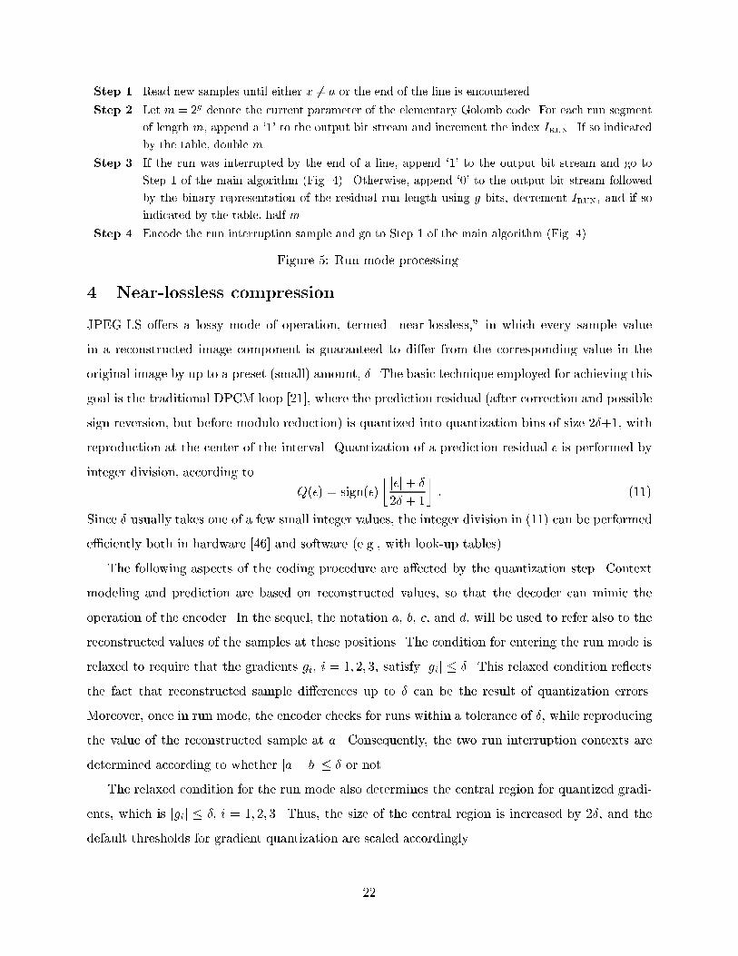
Step 1. Read new samples until either x 6= a or the end of the line is encountered.

Step 2. Let m = 2g denote the current parameter of the elementary Golomb code. For each run segment

of length m, append a `1' to the output bit stream and increment the index IRUN. If so indicated

by the table, double m.

Step 3. If the run was interrupted by the end of a line, append `1' to the output bit stream and go to

Step 1 of the main algorithm (Fig. 4). Otherwise, append `0' to the output bit stream followed

by the binary representation of the residual run length using g bits, decrement IRUN, and if so

indicated by the table, half m.

Step 4. Encode the run interruption sample and go to Step 1 of the main algorithm (Fig. 4).

Figure 5: Run mode processing.

4 Near-lossless compression

JPEG-LS o�ers a lossy mode of operation, termed \near-lossless," in which every sample value

in a reconstructed image component is guaranteed to di�er from the corresponding value in the

original image by up to a preset (small) amount, �. The basic technique employed for achieving this

goal is the traditional DPCM loop [21], where the prediction residual (after correction and possible

sign reversion, but before modulo reduction) is quantized into quantization bins of size 2�+1, with

reproduction at the center of the interval. Quantization of a prediction residual � is performed by

integer division, according to

Q(�) = sign(�)

� j�j+ �

2� + 1

�: (11)

Since � usually takes one of a few small integer values, the integer division in (11) can be performed

e�ciently both in hardware [46] and software (e.g., with look-up tables).

The following aspects of the coding procedure are a�ected by the quantization step. Context

modeling and prediction are based on reconstructed values, so that the decoder can mimic the

operation of the encoder. In the sequel, the notation a; b; c, and d, will be used to refer also to the

reconstructed values of the samples at these positions. The condition for entering the run mode is

relaxed to require that the gradients gi; i = 1; 2; 3, satisfy jgij � �. This relaxed condition re ects

the fact that reconstructed sample di�erences up to � can be the result of quantization errors.

Moreover, once in run mode, the encoder checks for runs within a tolerance of �, while reproducing

the value of the reconstructed sample at a. Consequently, the two run interruption contexts are

determined according to whether ja� bj � � or not.

The relaxed condition for the run mode also determines the central region for quantized gradi-

ents, which is jgij � �; i = 1; 2; 3. Thus, the size of the central region is increased by 2�, and the

default thresholds for gradient quantization are scaled accordingly.

22

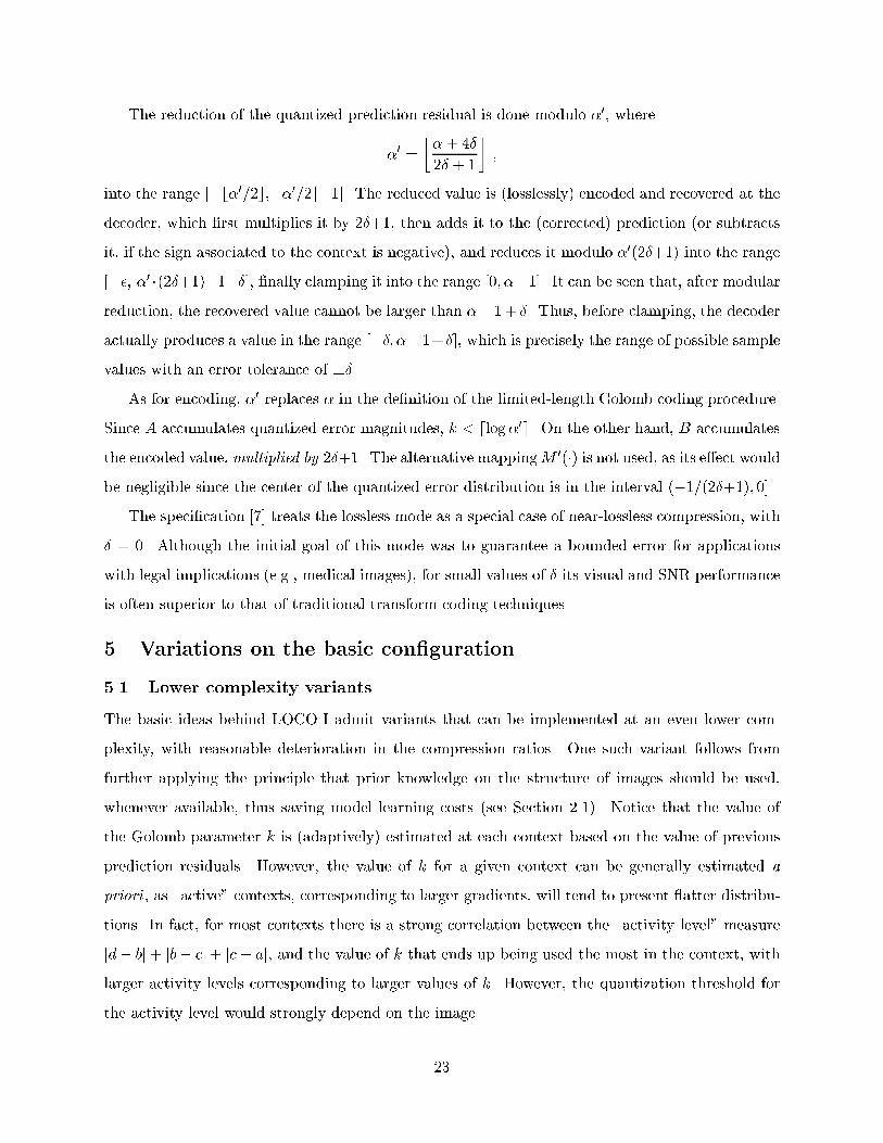
The reduction of the quantized prediction residual is done modulo �0, where

�0 =

��+ 4�

2� + 1

�;

into the range [�b�0=2c; d�0=2e�1]. The reduced value is (losslessly) encoded and recovered at the

decoder, which �rst multiplies it by 2�+1, then adds it to the (corrected) prediction (or subtracts

it, if the sign associated to the context is negative), and reduces it modulo �0(2�+1) into the range

[��; �0 �(2�+1)�1��], �nally clamping it into the range [0; ��1]. It can be seen that, after modular

reduction, the recovered value cannot be larger than �� 1+ �. Thus, before clamping, the decoder

actually produces a value in the range [��; ��1+�], which is precisely the range of possible sample

values with an error tolerance of ��.

As for encoding, �0 replaces � in the de�nition of the limited-length Golomb coding procedure.

Since A accumulates quantized error magnitudes, k < dlog�0e. On the other hand, B accumulates

the encoded value, multiplied by 2�+1. The alternative mappingM 0(�) is not used, as its e�ect would

be negligible since the center of the quantized error distribution is in the interval (�1=(2�+1); 0].

The speci�cation [7] treats the lossless mode as a special case of near-lossless compression, with

� = 0. Although the initial goal of this mode was to guarantee a bounded error for applications

with legal implications (e.g., medical images), for small values of � its visual and SNR performance

is often superior to that of traditional transform coding techniques.

5 Variations on the basic con�guration

5.1 Lower complexity variants

The basic ideas behind LOCO-I admit variants that can be implemented at an even lower com-

plexity, with reasonable deterioration in the compression ratios. One such variant follows from

further applying the principle that prior knowledge on the structure of images should be used,

whenever available, thus saving model learning costs (see Section 2.1). Notice that the value of

the Golomb parameter k is (adaptively) estimated at each context based on the value of previous

prediction residuals. However, the value of k for a given context can be generally estimated a

priori , as \active" contexts, corresponding to larger gradients, will tend to present atter distribu-

tions. In fact, for most contexts there is a strong correlation between the \activity level" measure

jd� bj+ jb� cj+ jc� aj, and the value of k that ends up being used the most in the context, with

larger activity levels corresponding to larger values of k. However, the quantization threshold for

the activity level would strongly depend on the image.

23

The above observation is related to an alternative interpretation of the modeling approach in

LOCO-I.10 Under this interpretation, the use of only jCj di�erent pre�x codes to encode context-

dependent distributions of prediction residuals, is viewed as a (dynamic) way of clustering condi-

tioning contexts. The clusters result from the use of a small family of codes, as opposed to a scheme

based on arithmetic coding, which would use di�erent arithmetic codes for di�erent distributions.

Thus, this aspect of LOCO-I can also be viewed as a realization of the basic paradigm proposed

and analyzed in [12] and also used in CALIC [17], in which a multiplicity of predicting contexts is

clustered into a few conditioning states. In the lower complexity alternative proposed in this sec-

tion, the clustering process is static, rather than dynamic. Such a static clustering can be obtained,

for example, by using the above activity level in lieu of A, and N = 3, to determine k in (8).

5.2 LOCO-A: an arithmetic coding extension

In this section, we present an arithmetic coding extension of LOCO-I, termed LOCO-A [47], which

has been adopted for a prospective extension of the baseline JPEG-LS standard (JPEG-LS Part 2).

The goal of this extension is to address the basic limitations that the baseline presents when dealing

with very compressible images (e.g., computer graphics, near-lossless mode with an error of �3 or

larger), due to the symbol-by-symbol coding approach, or with images that are very far from being

continuous-tone or have sparse histograms. Images of the latter type contain only a subset of the

possible sample values in each component, and the �xed predictor (1) would tend to concentrate the

value of the prediction residuals into a reduced set. However, prediction correction tends to spread

these values over the entire range, and even if that were not the case, the probability assignment

of a TSGD model in LOCO-I/JPEG-LS would not take advantage of the reduced alphabet.

In addition to better handling the special types of images mentioned above, LOCO-A closes,

in general, most of the (small) compression gap between JPEG-LS and the best published results

(see Section 6), while still preserving a certain complexity advantage due to simpler prediction and

modeling units, as described below.

LOCO-A is a natural extension of the JPEG-LS baseline, requiring the same bu�ering capability.

The context model and most of the prediction are identical to those in LOCO-I. The basic idea

behind LOCO-A follows from the alternative interpretation of the modeling approach in LOCO-I

discussed in Section 5.1. There, it was suggested that conditioning states could be obtained by

clustering contexts based on the value of the Golomb parameter k (thus grouping contexts with

10Xiaolin Wu, private communication.

24

similar conditional distributions). The resulting state-conditioned distributions can be arithmetic

encoded, thus relaxing the TSGD assumption, which would thus be used only as a means to form

the states. The relaxation of the TSGD assumption is possible due to the small number of states,

jCj = dlog�e+1, which enables the modeling of more parameters per state. In LOCO-A, this idea is

generalized to create higher resolution clusters based on the average magnitude A=N of prediction

residuals (as k is itself a function of A=N). Since, by de�nition, each cluster would include contexts

with very similar conditional distributions, this measure of activity level can be seen as a re�nement

of the \error energy" used in CALIC [17], and a further application of the paradigm of [12]. Activity

levels are also used in the ALCM algorithm [48].

Modeling in LOCO-A proceeds as in LOCO-I, collecting the same statistics at each context (the

\run mode" condition is used to de�ne a separate encoding state). The clustering is accomplished

by modifying (8) as follows:

k = minfk0 j 2k0=2N � Ag:

For 8-bit/sample images, 12 encoding states are de�ned: k = 0; k = 1; � � � ; k = 9; k > 9, and the

run state. A similar clustering is possible with other alphabet sizes.

Bias cancellation is performed as in LOCO-I, except that the correction value is tuned to produce

TSGDs with a shift s in the range �12� s < 1

2, instead of 0 � s < 1 (as the coding method that

justi�ed the negative fractional shift in LOCO-I is no longer used). In addition, regardless of the

computed correction value, the corrected prediction is incremented or decremented in the direction

of x̂MED until it is either a value that has already occurred in the image, or x̂MED. This modi�cation

alleviates the unwanted e�ects on images with sparse histograms, while having virtually no e�ect

on \regular" images. No bias cancellation is done in the run state. A \sign ip" borrowed from

the CALIC algorithm [17] is performed: if the bias count B is positive, then the sign of the error

is ipped. In this way, when distributions that are similar in shape but have opposite biases

are merged, the statistics are added \in phase." Finally, prediction errors are arithmetic-coded

conditioned on one of the 12 encoding states. Binary arithmetic coding is performed, following the

Golomb-based binarization strategy of [48]. For a state with index k, we choose the corresponding

binarization tree as the Golomb tree for the parameter 2dk=2e (the run state also uses k = 0).

Note that the modeling complexity in LOCO-A does not di�er signi�cantly from that of LOCO-

I. The only added complexity is in the determination of k (which, in software, can be done with a

simple modi�cation of the C \one-liner" used in LOCO-I), in the treatment of sparse histograms,

and in the use of a �fth sample in the causal template, West of a, as in [1]. The coding complexity,

25

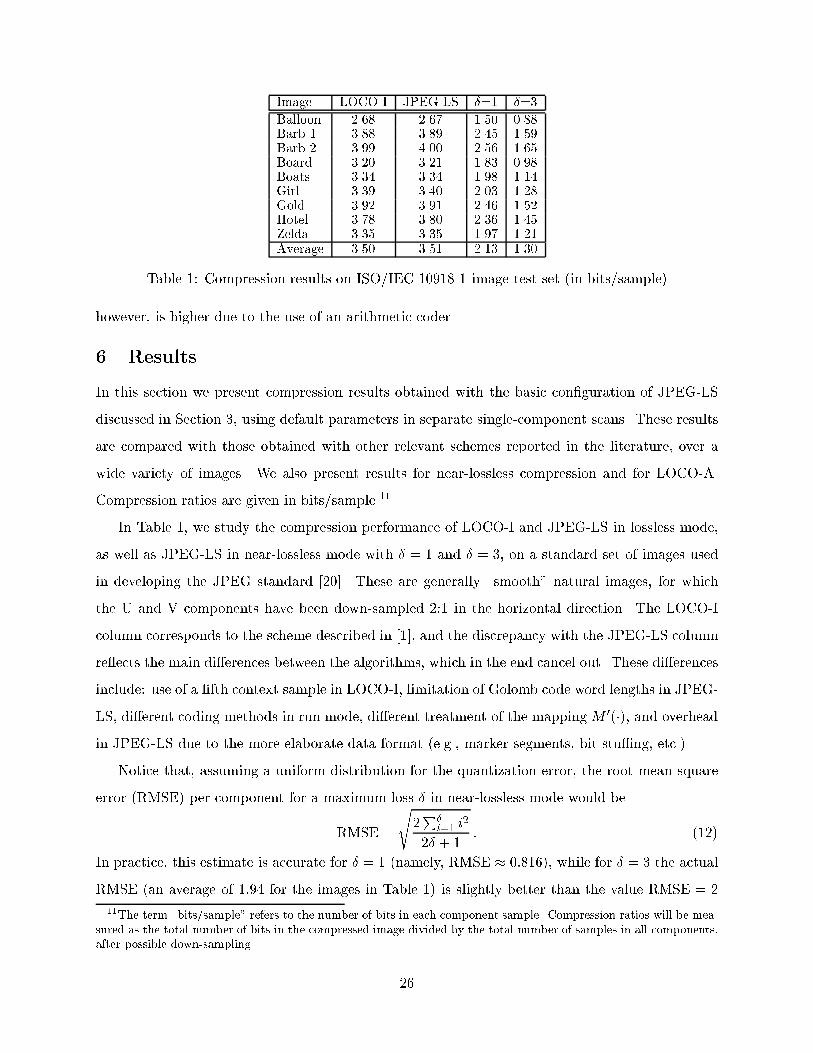
Image LOCO-I JPEG-LS �=1 �=3

Balloon 2.68 2.67 1.50 0.88Barb 1 3.88 3.89 2.45 1.59Barb 2 3.99 4.00 2.56 1.65Board 3.20 3.21 1.83 0.98Boats 3.34 3.34 1.98 1.14Girl 3.39 3.40 2.03 1.28Gold 3.92 3.91 2.46 1.52Hotel 3.78 3.80 2.36 1.45Zelda 3.35 3.35 1.97 1.21Average 3.50 3.51 2.13 1.30

Table 1: Compression results on ISO/IEC 10918-1 image test set (in bits/sample)

however, is higher due to the use of an arithmetic coder.

6 Results

In this section we present compression results obtained with the basic con�guration of JPEG-LS

discussed in Section 3, using default parameters in separate single-component scans. These results

are compared with those obtained with other relevant schemes reported in the literature, over a

wide variety of images. We also present results for near-lossless compression and for LOCO-A.

Compression ratios are given in bits/sample.11

In Table 1, we study the compression performance of LOCO-I and JPEG-LS in lossless mode,

as well as JPEG-LS in near-lossless mode with � = 1 and � = 3, on a standard set of images used

in developing the JPEG standard [20]. These are generally \smooth" natural images, for which

the U and V components have been down-sampled 2:1 in the horizontal direction. The LOCO-I

column corresponds to the scheme described in [1], and the discrepancy with the JPEG-LS column

re ects the main di�erences between the algorithms, which in the end cancel out. These di�erences

include: use of a �fth context sample in LOCO-I, limitation of Golomb code word lengths in JPEG-

LS, di�erent coding methods in run mode, di�erent treatment of the mappingM 0(�), and overhead

in JPEG-LS due to the more elaborate data format (e.g., marker segments, bit stu�ng, etc.).

Notice that, assuming a uniform distribution for the quantization error, the root mean square

error (RMSE) per component for a maximum loss � in near-lossless mode would be

RMSE =

s2P�

i=1 i2

2� + 1: (12)

In practice, this estimate is accurate for � = 1 (namely, RMSE � 0:816), while for � = 3 the actual

RMSE (an average of 1:94 for the images in Table 1) is slightly better than the value RMSE = 2

11The term \bits/sample" refers to the number of bits in each component sample. Compression ratios will be mea-

sured as the total number of bits in the compressed image divided by the total number of samples in all components,

after possible down-sampling.

26

estimated in (12). For such small values of �, the near-lossless coding approach is known to largely

outperform the (lossy) JPEG algorithm [20] in terms of RMSE at similar bit-rates [49]. For the

images in Table 1, typical RMSE values achieved by JPEG at similar bit-rates are 1:5 and 2:3,

respectively. On these images, JPEG-LS also outperforms the emerging wavelet-based JPEG 2000

standard [50] in terms of RMSE for bit-rates corresponding to � = 1.12 At bit-rates corresponding

to � > 2, however, the wavelet-based scheme yields far better RMSE. On the other hand, JPEG-LS

is considerably simpler and guarantees a maximum per-sample error.

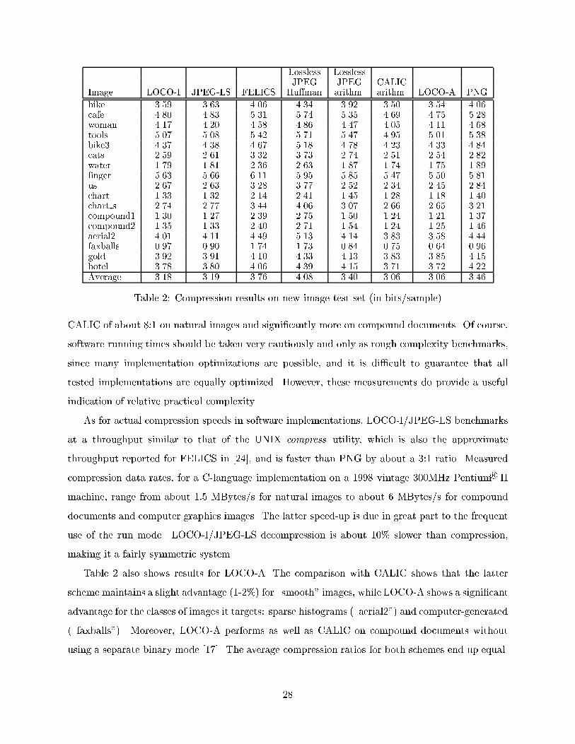
Table 2 shows (lossless) compression results of LOCO-I, JPEG-LS, and LOCO-A, compared

with other popular schemes. These include FELICS [24], for which the results were extracted from

[17], and the two versions of the original lossless JPEG standard [20], i.e., the strongest one based

on arithmetic coding, and the simplest one based on a �xed predictor followed by Hu�man coding

using \typical" tables [20]. This one-pass combination is probably the most widely used version

of the old lossless standard. The table also shows results for PNG, a popular �le format in which

lossless compression is achieved through prediction (in two passes) and a variant of LZ77 [51] (for

consistency, PNG was run in a plane-by-plane fashion). Finally, we have also included the arithmetic

coding version of the CALIC algorithm, which attains the best compression ratios among schemes

proposed in response to the Call for Contributions leading to JPEG-LS. These results are extracted

from [17]. The images in Table 2 are the subset of 8-bit/sample images from the benchmark set

provided in the above Call for Contributions. This is a richer set with a wider variety of images,

including compound documents, aerial photographs, scanned, and computer generated images.

The results in Table 2, as well as other comparisons presented in [1], show that LOCO-I/JPEG-

LS signi�cantly outperforms other schemes of comparable complexity (e.g., PNG, FELICS, JPEG-

Hu�man), and it attains compression ratios similar or superior to those of higher complexity

schemes based on arithmetic coding (e.g., Sunset CB9 [16], JPEG-Arithmetic). LOCO-I/JPEG-LS

is, on the average, within a few percentage points of the best available compression ratios (given,

in practice, by CALIC), at a much lower complexity level. Here, complexity was estimated by

measuring running times of software implementations made widely available by the authors of the

compared schemes.13 The experiments showed a compression time advantage for JPEG-LS over

12The default (9; 7) oating-point transform was used in these experiments, in the so-called \best mode" (non-

SNR-scalable). The progressive-to-lossless mode (reversible wavelet transform) yields worse results even at bit-rates

corresponding to � = 1.13The experiments were carried out with JPEG-LS executables available from http://www.hpl.hp.com/loco, and

CALIC executables available from ftp://ftp.csd.uwo.ca/pub/from wu as of the writing of this article. A common

platform for which both programs were available was used.

27

Lossless LosslessJPEG JPEG CALIC

Image LOCO-I JPEG-LS FELICS Hu�man arithm. arithm. LOCO-A PNG

bike 3.59 3.63 4.06 4.34 3.92 3.50 3.54 4.06cafe 4.80 4.83 5.31 5.74 5.35 4.69 4.75 5.28woman 4.17 4.20 4.58 4.86 4.47 4.05 4.11 4.68tools 5.07 5.08 5.42 5.71 5.47 4.95 5.01 5.38bike3 4.37 4.38 4.67 5.18 4.78 4.23 4.33 4.84cats 2.59 2.61 3.32 3.73 2.74 2.51 2.54 2.82water 1.79 1.81 2.36 2.63 1.87 1.74 1.75 1.89�nger 5.63 5.66 6.11 5.95 5.85 5.47 5.50 5.81us 2.67 2.63 3.28 3.77 2.52 2.34 2.45 2.84chart 1.33 1.32 2.14 2.41 1.45 1.28 1.18 1.40chart s 2.74 2.77 3.44 4.06 3.07 2.66 2.65 3.21compound1 1.30 1.27 2.39 2.75 1.50 1.24 1.21 1.37compound2 1.35 1.33 2.40 2.71 1.54 1.24 1.25 1.46aerial2 4.01 4.11 4.49 5.13 4.14 3.83 3.58 4.44faxballs 0.97 0.90 1.74 1.73 0.84 0.75 0.64 0.96gold 3.92 3.91 4.10 4.33 4.13 3.83 3.85 4.15hotel 3.78 3.80 4.06 4.39 4.15 3.71 3.72 4.22Average 3.18 3.19 3.76 4.08 3.40 3.06 3.06 3.46

Table 2: Compression results on new image test set (in bits/sample)

CALIC of about 8:1 on natural images and signi�cantly more on compound documents. Of course,

software running times should be taken very cautiously and only as rough complexity benchmarks,

since many implementation optimizations are possible, and it is di�cult to guarantee that all

tested implementations are equally optimized. However, these measurements do provide a useful

indication of relative practical complexity.

As for actual compression speeds in software implementations, LOCO-I/JPEG-LS benchmarks

at a throughput similar to that of the UNIX compress utility, which is also the approximate

throughput reported for FELICS in [24], and is faster than PNG by about a 3:1 ratio. Measured

compression data rates, for a C-language implementation on a 1998 vintage 300MHz Pentium R II

machine, range from about 1:5 MBytes/s for natural images to about 6 MBytes/s for compound

documents and computer graphics images. The latter speed-up is due in great part to the frequent

use of the run mode. LOCO-I/JPEG-LS decompression is about 10% slower than compression,

making it a fairly symmetric system.

Table 2 also shows results for LOCO-A. The comparison with CALIC shows that the latter

scheme maintains a slight advantage (1-2%) for \smooth" images, while LOCO-A shows a signi�cant

advantage for the classes of images it targets: sparse histograms (\aerial2") and computer-generated

(\faxballs"). Moreover, LOCO-A performs as well as CALIC on compound documents without

using a separate binary mode [17]. The average compression ratios for both schemes end up equal.

28

It is also interesting to compare LOCO-A with the JBIG algorithm [52] as applied in [53] to

multi-level images (i.e., bit-plane coding of Gray code representation). In [53], the components

of the images of Table 1 are reduced to amplitude precisions below 8 bits/sample, in order to

provide data for testing how algorithm performances scale with precision. LOCO-A outperforms

JBIG for all precisions above 3 bits/sample: for example, at 4 bits/sample (i.e., considering down-

sampling, a total of 8 bits/pixel), the average image size for LOCO-A is 1:38 bits/pixel, whereas

the average size reported in [53] for JBIG is 1:42 bits/pixel. At 3 bits/sample, the relation is

reverted: the averages are 0:86 and 0:83 bits/pixel, respectively. While the JPEG-LS baseline

outperforms JBIG by 11% on the average at 8 bits/sample for the images of Table 1 (the average

compressed image size reported in [53] is 3:92 bits/sample), the relative performance deteriorates

rapidly below 6 bits/sample, which is the minimum precision for which baseline JPEG-LS still

yields better compression ratios (3:68 against 3:87 bits/pixel). Thus, LOCO-A indeed addresses

the basic limitations that the baseline presents when dealing with very compressible images.

Software implementations of JPEG-LS for various platforms are available at the web site

http://www.hpl.hp.com/loco/. The organizations holding patents covering aspects of JPEG-

LS have agreed to allow payment-free licensing of these patents for use in the standard.

Appendix: Other features of the standard

Bit stream. The compressed data format for JPEG-LS closely follows the one speci�ed for

JPEG [20]. The same high level syntax applies, with the bit stream organized into frames, scans,

and restart intervals within a scan, markers specifying the various structural parts, and marker seg-

ments specifying the various parameters. New marker assignments are compatible with [20]. One

di�erence, however, is the existence of default values for many of the JPEG-LS coding parameters

(e.g., gradient quantization thresholds, reset threshold), with marker segments used to override

these values. In addition, the method for easy detection of marker segments di�ers from the one

in [20]. Speci�cally, a single byte of coded data with the hexadecimal value `FF' is followed with

the insertion of a single bit `0,' which occupies the most signi�cant bit position of the next byte.

This technique is based on the fact that all markers start with an `FF' byte, followed by a bit `1.'

Color images. For encoding images with more than one component (e.g., color images), JPEG-LS

supports combinations of single-component and multi-component scans. Section 3 describes the

encoding process for a single-component scan. For multi-component scans, a single set of context

counters (namely, A; B; C, and N for regular mode contexts) is used across all components in the

29

scan. Prediction and context determination are performed as in the single component case, and are

component independent. Thus, the use of possible correlation between color planes is limited to

sharing statistics, collected from all planes. For some color spaces (e.g., RGB), good decorrelation

can be obtained through simple lossless color transforms as a pre-processing step to JPEG-LS. For

example, compressing the (R-G,G,B-G) representations of the images of Table 1, with di�erences

taken modulo the alphabet size � in the interval [�b�=2c; d�=2e�1], yields savings between 25

and 30% over compressing the respective RGB representations. These savings are similar to those

obtained with more elaborate schemes which do not assume prior knowledge of the color space [26].

Given the variety of color spaces, the standardization of speci�c �lters was considered beyond the

scope of JPEG-LS, and color transforms are handled at the application level.

In JPEG-LS, the data in a multi-component scan can be interleaved either by lines (line-

interleaved mode) or by samples (sample-interleaved mode). In line-interleaved mode, assuming an

image that is not sub-sampled in the vertical direction, a full line of each component is encoded

before starting the encoding of the next line (for images sub-sampled in the vertical direction, more

than one line from a component are interleaved before starting with the next component). The

index to the table used to adapt the elementary Golomb code in run mode is component-dependent.

In sample-interleaved mode, one sample from each component is processed in turn, so that

all components which belong to the same scan must have the same dimensions. The runs are

common to all the components in the scan, with run mode selected only when the corresponding

condition is satis�ed for all the components. Likewise, a run is interrupted whenever so dictated

by any of the components. Thus, a single run length, common to all components, is encoded. This

approach is convenient for images in which runs tend to be synchronized between components (e.g.,

synthetic images), but should be avoided in cases where run statistics di�er signi�cantly across

components, since a component may systematically cause run interruptions for another component

with otherwise long runs. For example, in a CMYK representation, the runs in the K plane tend

to be longer than in the other planes, so it is best to encode the K plane in a di�erent scan.

The performance of JPEG-LS, run in line-interleaved mode on the images of Table 2, is very

similar to that of the component-by-component mode shown in the table. We observed a maximum

compression ratio deterioration of 1% on \gold" and \hotel," and a maximum improvement of 1% on

\compound1." In sample-interleaved mode, however, the deterioration is generally more signi�cant

(3 to 5% in many cases), but with a 3 to 4% improvement on compound documents.

30

Palletized images. The JPEG-LS data format also provides tools for encoding palletized images

in an appropriate index space (i.e., as an array of indices to a palette table), rather than in the

original color space. To this end, the decoding process may be followed by a so-called sample-

mapping procedure, which maps each decoded sample value (e.g., and 8-bit index) to a reconstructed

sample value (e.g., an RGB triplet) by means of mapping tables. Appropriate syntax is de�ned to

allow embedding of these tables in the JPEG-LS bit stream.

Many of the assumptions for the JPEG-LS model, targeted at continuous-tone images, do not

hold when compressing an array of indices. However, an appropriate reordering of the palette table

can sometimes alleviate this de�ciency. Some heuristics are known that produce good results at low

complexity, without using image statistics. For example, [54] proposes to arrange the palette colors

in increasing order of luminance value, so that samples that are close in space in a smooth image

will tend to be close in color and in luminance. Using this reordering, JPEG-LS outperforms PNG

by about 6% on palletized versions of the images \lena" and \gold". On the other hand, PNG may

be advantageous for dithered, halftoned, and some graphic images for which LZ-type methods are

better suited. JPEG-LS does not specify a particular heuristic for palette ordering.

The sample-mapping procedure can also be used to alleviate the problem of \sparse histograms"

mentioned in Section 5.2, by mapping the sparse samples to a contiguous set. This, however,

assumes a prior knowledge of the histogram sparseness not required by the LOCO-A solution.

Acknowledgments. Many thanks to H. Kajiwara, G. Langdon, D. Lee, N. Memon, F. Ono, E.

Ordentlich, M. Rabbani, D. Speck, I. Ueno, X. Wu, and T. Yoshida for useful discussions.

References

[1] M. J. Weinberger, G. Seroussi, and G. Sapiro, \LOCO-I: A low complexity, context-based, lossless

image compression algorithm," in Proc. 1996 Data Compression Conference, (Snowbird, Utah, USA),

pp. 140{149, Mar. 1996.

[2] I. Ueno and F. Ono, \Proposed modi�cation of LOCO-I for its improvement of the performance."

ISO/IEC JTC1/SC29/WG1 document N297, Feb. 1996.

[3] M. J. Weinberger, G. Seroussi, and G. Sapiro, \Fine-tuning the baseline." ISO/IEC JTC1/SC29/WG1

document N341, June 1996.

[4] M. J. Weinberger, G. Seroussi, and G. Sapiro, \E�ects of resets and number of contexts on the baseline."

ISO/IEC JTC1/SC29/WG1 document N386, June 1996.

[5] M. J. Weinberger, G. Seroussi, and G. Sapiro, \Palettes and sample mapping in JPEG-LS." ISO/IEC

JTC1/SC29/WG1 document N412, Nov. 1996.

[6] M. J. Weinberger, G. Seroussi, G. Sapiro, and E. Ordentlich, \JPEG-LS with limited-length code

words." ISO/IEC JTC1/SC29/WG1 document N538, July 1997.

31

[7] ISO/IEC 14495-1, ITU Recommendation T.87, \Information technology - Lossless and near-lossless

compression of continuous-tone still images," 1999.

[8] M. J. Weinberger, G. Seroussi, and G. Sapiro, \LOCO-I: A low complexity lossless image compression

algorithm." ISO/IEC JTC1/SC29/WG1 document N203, July 1995.

[9] J. Rissanen and G. G. Langdon, Jr., \Universal modeling and coding," IEEE Trans. Inform. Theory,

vol. IT-27, pp. 12{23, Jan. 1981.

[10] J. Rissanen, \Generalized Kraft inequality and arithmetic coding," IBM Jl. Res. Develop., vol. 20 (3),

pp. 198{203, May 1976.

[11] M. J. Weinberger, J. Rissanen, and R. B. Arps, \Applications of universal context modeling to lossless

compression of gray-scale images," IEEE Trans. Image Processing, vol. 5, pp. 575{586, Apr. 1996.

[12] M. J. Weinberger and G. Seroussi, \Sequential prediction and ranking in universal context modeling

and data compression," IEEE Trans. Inform. Theory, vol. 43, pp. 1697{1706, Sept. 1997. Preliminary

version presented at the 1994 IEEE Intern'l Symp. on Inform. Theory, Trondheim, Norway, July 1994.

[13] S. Todd, G. G. Langdon, Jr., and J. Rissanen, \Parameter reduction and context selection for compres-

sion of the gray-scale images," IBM Jl. Res. Develop., vol. 29 (2), pp. 188{193, Mar. 1985.

[14] G. G. Langdon, Jr., A. Gulati, and E. Seiler, \On the JPEG model for lossless image compression," in

Proc. 1992 Data Compression Conference, (Snowbird, Utah, USA), pp. 172{180, Mar. 1992.

[15] G. G. Langdon, Jr. and M. Manohar, \Centering of context-dependent components of prediction error

distributions," in Proc. SPIE (Applications of Digital Image Processing XVI), vol. 2028, pp. 26{31, 1993.

[16] G. G. Langdon, Jr. and C. A. Haidinyak, \Experiments with lossless and virtually lossless image com-

pression algorithms," in Proc. SPIE, vol. 2418, pp. 21{27, Feb. 1995.

[17] X. Wu and N. D. Memon, \Context-based, adaptive, lossless image coding," IEEE Trans. Commun.,

vol. 45 (4), pp. 437{444, Apr. 1997.

[18] X. Wu, \E�cient lossless compression of continuous-tone images via context selection and quantization,"

IEEE Trans. Image Processing, vol. IP-6, pp. 656{664, May 1997.

[19] B. Meyer and P. Tischer, \TMW { A new method for lossless image compression," in Proc. of the 1997

International Picture Coding Symposium (PCS97), (Berlin, Germany), Sept. 1997.

[20] ISO/IEC 10918-1, ITU Recommendation T.81, \Digital compression and coding of continuous tone still

images - Requirements and guidelines," Sept. 1993.

[21] A. Netravali and J. O. Limb, \Picture coding: A review," Proc. IEEE, vol. 68, pp. 366{406, 1980.

[22] D. Hu�man, \A method for the construction of minimum redundancy codes," Proc. IRE, vol. 40,

pp. 1098{1101, 1952.

[23] M. Feder and N. Merhav, \Relations between entropy and error probability," IEEE Trans. Inform.

Theory, vol. IT-40, pp. 259{266, Jan. 1994.

[24] P. G. Howard and J. S. Vitter, \Fast and e�cient lossless image compression," in Proc. 1993 Data

Compression Conference, (Snowbird, Utah, USA), pp. 351{360, Mar. 1993.

[25] X. Wu, W.-K. Choi, and N. D. Memon, \Lossless interframe image compression via context modeling,"

in Proc. 1998 Data Compression Conference, (Snowbird, Utah, USA), pp. 378{387, Mar. 1998.

[26] R. Barequet and M. Feder, \SICLIC: A simple inter-color lossless image coder," in Proc. 1999 Data

Compression Conference, (Snowbird, Utah, USA), pp. 501{510, Mar. 1999.

[27] J. Rissanen, Stochastic Complexity in Statistical Inquiry. New Jersey, London: World Scienti�c, 1989.

[28] J. Rissanen, \Universal coding, information, prediction, and estimation," IEEE Trans. Inform. Theory,

vol. IT-30, pp. 629{636, July 1984.

[29] N. Merhav, M. Feder, and M. Gutman, \Some properties of sequential predictors for binary Markov

sources," IEEE Trans. Inform. Theory, vol. IT-39, pp. 887{892, May 1993.

[30] M. J. Weinberger, J. Rissanen, and M. Feder, \A universal �nite memory source," IEEE Trans. Inform.

Theory, vol. IT-41, pp. 643{652, May 1995.

32

[31] P. A. Maragos, R. W. Schafer, and R. M. Mersereau, \Two-dimensional linear predictive coding and its

application to adaptive predictive coding of images," IEEE Trans. ASSP, vol. ASSP-32, pp. 1213{1229,

Dec. 1984.

[32] S. W. Golomb, \Run-length encodings," IEEE Trans. Inform. Theory, vol. IT-12, pp. 399{401, 1966.

[33] N. Merhav, G. Seroussi, and M. J. Weinberger, \Coding of sources with two-sided geometric distributions

and unknown parameters," 1999. To appear in IEEE Trans. Inform. Theory. Available as part of

Technical Report No. HPL-98-70, Apr. 1998, Hewlett-Packard Laboratories.

[34] N. Merhav, G. Seroussi, and M. J. Weinberger, \Modeling and low-complexity adaptive coding for image

prediction residuals," in Proc. of the 1996 Int'l Conference on Image Processing, vol. II, (Lausanne,

Switzerland), pp. 353{356, Sept. 1996.

[35] N. Merhav, G. Seroussi, and M. J. Weinberger, \Optimal pre�x codes for sources with two-sided geo-

metric distributions," 1999. To appear in IEEE Trans. Inform. Theory. Available as part of Technical

Report No. HPL-98-70, Apr. 1998, Hewlett-Packard Laboratories.

[36] R. Ohnishi, Y. Ueno, and F. Ono, \The e�cient coding scheme for binary sources," IECE of Japan,

vol. 60-A, pp. 1114{1121, Dec. 1977. (In Japanese).

[37] S. A. Martucci, \Reversible compression of HDTV images using median adaptive prediction and arith-

metic coding," in Proc. IEEE Intern'l Symp. on Circuits and Syst., pp. 1310{1313, IEEE Press, 1990.

[38] G. Seroussi and M. J. Weinberger, \On adaptive strategies for an extended family of Golomb-type

codes," in Proc. 1997 Data Compression Conference, (Snowbird, Utah, USA), pp. 131{140, Mar. 1997.

[39] R. F. Rice, \Some practical universal noiseless coding techniques - parts I-III," Tech. Rep. JPL-79-22,

JPL-83-17, and JPL-91-3, Jet Propulsion Laboratory, Pasadena, CA, Mar. 1979, Mar. 1983, Nov. 1991.

[40] Digital Imaging Group, \FlashPix format speci�cation." Version 1.0.1, July 1997.

[41] D. E. Knuth, \Dynamic Hu�man coding," J. Algorithms, vol. 6, pp. 163{180, 1985.

[42] R. Gallager and D. V. Voorhis, \Optimal source codes for geometrically distributed integer alphabets,"

IEEE Trans. Inform. Theory, vol. IT-21, pp. 228{230, Mar. 1975.

[43] J. Teuhola, \A compression method for clustered bit-vectors," Information Processing Letters, vol. 7,

pp. 308{311, Oct. 1978.

[44] G. G. Langdon, Jr., \An adaptive run-length coding algorithm," IBM Technical Disclosure Bulletin,

vol. 26, pp. 3783{3785, Dec. 1983.

[45] E. Ordentlich, M. J. Weinberger, and G. Seroussi, \A low complexity modeling approach for embedded

coding of wavelet coe�cients," in Proc. 1998 Data Compression Conference, (Snowbird, Utah, USA),

pp. 408{417, Mar. 1998.

[46] S.-Y. Li, \Fast constant division routines," IEEE Trans. Computers, vol. C-34, pp. 866{869, Sept. 1985.

[47] M. J. Weinberger, G. Seroussi, and G. Sapiro, \LOCO-A: an arithmetic coding extension of LOCO-I."

ISO/IEC JTC1/SC29/WG1 document N342, June 1996.

[48] D. Speck, \Activity level classi�cation model (ALCM)." A proposal submitted in response to the Call

for Contributions for ISO/IEC JTC 1.29.12, 1995.

[49] F. Ono and I. Ueno, \Evaluation of JPEG-DCT as a near-lossless function." ISO/IEC JTC1/SC29/WG1

document N207, June 1995.

[50] ISO/IEC JTC1/SC29/WG1 document N1422, \JPEG 2000 VM 5.02," Sept. 1999.

[51] J. Ziv and A. Lempel, \A universal algorithm for sequential data compression," IEEE Trans. Inform.

Theory, vol. IT-23, pp. 337{343, May 1977.

[52] ISO/IEC 11544, CCITT T.82, \Progressive bi-level image compression," 1993.

[53] R. B. Arps and T. K. Truong, \Comparison of international standards for lossless still image compres-

sion," Proceedings of the IEEE, vol. 82, pp. 889{899, June 1994.

[54] A. Zaccarin and B. Liu, \A novel approach for coding color quantized images," IEEE Trans. Image

Processing, vol. IP-2, pp. 442{453, Oct. 1993.

33