THE LORELIA RESIDUAL TEST - uni-bremen.deelib.suub.uni-bremen.de/diss/docs/00011612.pdf · truly as...
206
THE LORELIA RESIDUAL TEST A NEW OUTLIER IDENTIFICATION TEST FOR METHOD COMPARISON STUDIES Dissertation Thesis Submitted to the Faculty of Mathematics and Informatics of the University of Bremen in Partial Fulfillment of the Requirements for the Degree of Doctor of Natural Sciences (Dr. rer. nat.) by Geraldine Rauch August 2009 In Cooperation with Roche Diagnostics GmbH First Reviewer: Prof. Dr. J¨ urgen Timm, University of Bremen Second Reviewer: Dr. Andrea Geistanger, Roche Diagnostics GmbH Supervising Tutor: Dr. Christoph Berding, Roche Diagnostics GmbH
Transcript of THE LORELIA RESIDUAL TEST - uni-bremen.deelib.suub.uni-bremen.de/diss/docs/00011612.pdf · truly as...

THE LORELIA RESIDUAL TEST
A NEW OUTLIER IDENTIFICATION TEST FOR METHOD
COMPARISON STUDIES
Dissertation Thesis
Submitted to the Faculty of Mathematics and Informatics of the University of Bremen
in Partial Fulfillment of the Requirements for the Degree of
Doctor of Natural Sciences (Dr. rer. nat.)
by Geraldine Rauch
August 2009
In Cooperation with
Roche Diagnostics GmbH
First Reviewer: Prof. Dr. Jurgen Timm, University of Bremen
Second Reviewer: Dr. Andrea Geistanger, Roche Diagnostics GmbH
Supervising Tutor: Dr. Christoph Berding, Roche Diagnostics GmbH

Acknowledgments
This thesis would not have been possible without
the helpful support, the motivating advises and the
constructive guidance of my supervisors Prof. Dr.
Jurgen Timm, Dr. Christoph Berding and Dr. Andrea
Geistanger to whom I owe my special gratitude.
Moreover, I want to thank the whole department
of Biostatistic of Roche Diagnostics Penzberg, as I have
never worked in a more friendly and helpful atmosphere.
My special thanks go to my wonderful family,
who always encouraged and supported me.
Finally, I want to thank my friend Peter Gebauer,
who helped me to keep my calm.
Geraldine Rauch

Contents
1 Introduction 1
2 Overview of the Theory of Outliers 42.1 History of Research . . . . . . . . . . . . . . . . . . . . . . . . . . . . . . . 4
2.2 Motivation of Outlier Identification and Robust Statistical Methods . . . . . . 5
2.3 An Informal Definition of Outliers . . . . . . . . . . . . . . . . . . . . . . . 6
2.3.1 Outliers, Extreme Values and Contaminants . . . . . . . . . . . . . . 7
2.3.2 The Diversity of Extremeness . . . . . . . . . . . . . . . . . . . . . 12
2.3.2.1 Extremeness with Respect to the Majority of Data . . . . . 12
2.3.2.2 The Importance of Underlying Statistical Assumptions . . 13
2.3.2.3 Extremeness in Multivariate Datasets . . . . . . . . . . . . 14
2.3.2.4 Ambiguity of Extreme Values . . . . . . . . . . . . . . . . 15
2.4 A Short Classification of Outlier Candidates . . . . . . . . . . . . . . . . . . 17
2.4.1 The Statistical Assumptions . . . . . . . . . . . . . . . . . . . . . . 17
2.4.2 Causes for Extreme Values . . . . . . . . . . . . . . . . . . . . . . . 18
2.4.3 Different Goals of Outlier Identification . . . . . . . . . . . . . . . . 18
3 Different Concepts for Outlier Tests 203.1 Classification of Outlier Tests . . . . . . . . . . . . . . . . . . . . . . . . . . 20
3.1.1 Tests for a Fixed Number of Outlier Candidates . . . . . . . . . . . . 20
3.1.2 Tests to Check the Whole Dataset . . . . . . . . . . . . . . . . . . . 21
3.2 Formulation of the Test Hypotheses . . . . . . . . . . . . . . . . . . . . . . 23
3.2.1 Discordancy Tests . . . . . . . . . . . . . . . . . . . . . . . . . . . 23
3.2.2 Incorporation of Outliers . . . . . . . . . . . . . . . . . . . . . . . . 24
3.2.2.1 The Inherent Hypotheses . . . . . . . . . . . . . . . . . . 24
3.2.2.2 The Deterministic Hypotheses . . . . . . . . . . . . . . . 24
3.2.2.3 The Mixed Model Alternative . . . . . . . . . . . . . . . . 25
3.3 Problems and Test Limitations . . . . . . . . . . . . . . . . . . . . . . . . . 25

3.3.1 The Masking Effect . . . . . . . . . . . . . . . . . . . . . . . . . . . 25
3.3.2 The Swamping Effect . . . . . . . . . . . . . . . . . . . . . . . . . . 26
3.3.3 The Leverage Effect . . . . . . . . . . . . . . . . . . . . . . . . . . 27
4 Evaluation of Method Comparison Studies 304.1 Comparison by the Method Differences . . . . . . . . . . . . . . . . . . . . 30
4.1.1 The Absolute Differences . . . . . . . . . . . . . . . . . . . . . . . 31
4.1.2 The Relative Differences . . . . . . . . . . . . . . . . . . . . . . . . 32
4.2 Comparison with Regression Analysis . . . . . . . . . . . . . . . . . . . . . 36
4.2.1 Robust Regression Methods . . . . . . . . . . . . . . . . . . . . . . 37
4.2.1.1 Deming Regression . . . . . . . . . . . . . . . . . . . . . 38
4.2.1.2 Principal Component Analysis . . . . . . . . . . . . . . . 39
4.2.1.3 Standardized Principal Component Analysis . . . . . . . . 39
4.2.1.4 Passing-Bablok Regression . . . . . . . . . . . . . . . . . 41
5 Common Outlier Tests for MCS 435.1 Outlier Tests based on Method Differences . . . . . . . . . . . . . . . . . . . 44
5.1.1 Problems and Limitations . . . . . . . . . . . . . . . . . . . . . . . 45
5.2 Outlier Test based on Regression . . . . . . . . . . . . . . . . . . . . . . . . 45
5.2.1 Problems and Limitations . . . . . . . . . . . . . . . . . . . . . . . 46
6 The New LORELIA Residual Test 486.1 Statistical Assumptions for the New Test . . . . . . . . . . . . . . . . . . . . 49
6.2 The Concept of Local Confidence Intervals . . . . . . . . . . . . . . . . . . 50
6.3 How to Weight - Newly Developed Criteria . . . . . . . . . . . . . . . . . . 52
6.3.1 Historical Background - Basic Ideas . . . . . . . . . . . . . . . . . . 52
6.3.1.1 Problems and Limitations . . . . . . . . . . . . . . . . . . 53
6.3.2 New Concepts for Weight Construction . . . . . . . . . . . . . . . . 57
6.3.2.1 Construction of a Local Estimator . . . . . . . . . . . . . . 57
6.3.2.2 Construction of an Outlier Robust Estimator . . . . . . . . 58
6.3.2.3 Invariance under Axes Scaling . . . . . . . . . . . . . . . 58
6.3.2.4 The Meaning of the Local Data Information Density . . . . 59
6.3.2.5 The Co-Domain of the Weights . . . . . . . . . . . . . . . 59
6.4 The Weights for the LORELIA Residual Test . . . . . . . . . . . . . . . . . 60
6.4.1 Definition of the Distance Measure . . . . . . . . . . . . . . . . . . 60
6.4.2 Definition of a Reliability Measure . . . . . . . . . . . . . . . . . . . 64
6.5 Definition of the LORELIA Residual Test . . . . . . . . . . . . . . . . . . . 67
7 Performance of the New LORELIA Residual Test 697.1 The LORELIA Residual Test in Comparison to Common Outlier Tests . . . . 71
7.1.1 Performance Comparison for Real Data Situations . . . . . . . . . . 72
7.1.1.1 No Suspicious Values . . . . . . . . . . . . . . . . . . . . 72
7.1.1.2 One Outlier Candidate . . . . . . . . . . . . . . . . . . . . 75
7.1.1.3 Uncertain Outlier Situation . . . . . . . . . . . . . . . . . 79
7.1.1.4 Decreasing Residual Variances . . . . . . . . . . . . . . . 82
7.1.1.5 Very Inhomogeneous Data Distribution . . . . . . . . . . . 84
7.1.1.6 Conclusion . . . . . . . . . . . . . . . . . . . . . . . . . . 88
7.1.2 Proof of Performance Superiority for an Exemplary Data Model . . . 88
7.1.3 Performance Comparison for Simulated Datasets . . . . . . . . . . . 95
7.1.3.1 Simulation Models . . . . . . . . . . . . . . . . . . . . . . 96
7.1.3.2 Evaluation of the Simulation Results . . . . . . . . . . . . 99
7.1.3.2.1 Actual Type 1 Error Rates . . . . . . . . . . . . . 100
7.1.3.2.2 True Positive and False Positive Test Results . . . 100
7.1.3.3 General Observations and Conclusions . . . . . . . . . . . 107
7.2 Influence of the Outlier Position on its Identification . . . . . . . . . . . . . . 109
7.2.1 Simulation Models . . . . . . . . . . . . . . . . . . . . . . . . . . . 110
7.2.2 Homogeneous Data Distribution . . . . . . . . . . . . . . . . . . . . 112
7.2.2.1 Constant Residual Variance . . . . . . . . . . . . . . . . . 112
7.2.2.1.1 Expected Results . . . . . . . . . . . . . . . . . 112
7.2.2.1.2 Observed Results . . . . . . . . . . . . . . . . . 115
7.2.2.2 Constant Coefficient of Variance . . . . . . . . . . . . . . 118
7.2.2.2.1 Expected Results . . . . . . . . . . . . . . . . . 118
7.2.2.2.2 Observed Results . . . . . . . . . . . . . . . . . 118
7.2.3 Inhomogeneous Data Distribution . . . . . . . . . . . . . . . . . . . 120
7.2.3.1 Constant Residual Variance . . . . . . . . . . . . . . . . . 120
7.2.3.1.1 Expected Results . . . . . . . . . . . . . . . . . 121
7.2.3.1.2 Observed Results . . . . . . . . . . . . . . . . . 121
7.2.3.2 Constant Coefficient of Variance . . . . . . . . . . . . . . 123
7.2.3.2.1 Expected Results . . . . . . . . . . . . . . . . . 123
7.2.3.2.2 Observed Results . . . . . . . . . . . . . . . . . 124
7.3 How to Deal with Complex Residual Variance Models . . . . . . . . . . . . 126
7.4 Considerations on the Alpha Adjustment . . . . . . . . . . . . . . . . . . . . 130
7.5 Summary of the Performance Results . . . . . . . . . . . . . . . . . . . . . 130

8 Conclusions and Outlook 133
A Software Development and Documentation 137
B Test Results of Section 7.1.3 140B.1 Constant Residual Variance . . . . . . . . . . . . . . . . . . . . . . . . . . . 140
B.2 Constant Coefficient of Variance . . . . . . . . . . . . . . . . . . . . . . . . 154
B.3 Non Constant Coefficient of Variance . . . . . . . . . . . . . . . . . . . . . 168
Symbols 182
List of Figures 184
List of Tables 193
Bibliography 194

Chapter 1
Introduction
In this work, a new outlier identification test for method comparison studies based on ro-
bust linear regression is proposed in order to overcome the special problem of heteroscedastic
residual variances.
Method comparison studies are performed in order to prove equivalence or to detect system-
atic differences between two measurement methods, instruments or diagnostic tests. They are
often evaluated by linear regression methods. As the existence of outliers within the dataset
can bias non robust regression estimators, robust linear regression methods should be pre-
ferred. In this work, the use of Passing-Bablok regression is suggested which is described in
[Passing, Bablok, 1983], [Passing, Bablok, 1984] and [Bablok et al. 1988]. Passing-Bablok
regression is a very outlier resistant procedure which takes random errors in both variables
into account. Moreover, the measurement error variances are not required to be constant, so
Passing-Bablok regression is still appropriate if the error variances depend on the true con-
centration which is a common situation for many laboratory datasets.
Beside the use of robust regression methods, it is strongly recommended to scan the dataset
for outliers with an appropriate outlier test, as outliers can indicate serious errors in the mea-
surement process or problems with the data handling. Therefore, outliers should always be
carefully examined and reported in order to detect possible error sources and to avoid misin-
terpretations.
If method comparison is evaluated by a robust regression method (here Passing-Bablok), out-
liers will correspond to measurement values with surprisingly large orthogonal residuals. A
possible approach for the identification of outliers is the construction of confidence intervals
for the orthogonal residuals which will serve as outlier limits. These confidence intervals will
depend on the underlying residual variance, which has to be estimated. Note that only robust
variance estimators are appropriate in this context as otherwise existing outliers will bias the
estimate.
1

CHAPTER 1. INTRODUCTION 2
Common outlier tests for method comparison studies are based on global, robust outlier limits
for the residuals of a regression analysis or for the measurement distances. In the work of
[Wadsworth, 1990], global, robust outlier limits of the form
med(·)± q ·mad68(·)are proposed, where q correspond to some predefined quantile. This approach can be applied
to any of the comparison measures proposed above. However it requires that the measure-
ment error variances or the residual variances, respectively, remain constant over the mea-
suring range. If the variances follow a simple model, for example if they are proportional
to the true concentration (constant coefficient of variance) the same concepts can be applied
after an appropriate data transformation. However, in many practical applications the error
variances or residual variances, respectively, do not follow a simple model - they are neither
constant nor proportional to the true concentration and the underlying variance model is un-
known. In this case none of the transformation methods proposed in the literature will fit and
common robust variance estimators as proposed in [Wadsworth, 1990] will not be appropriate.
The new LORELIA Residual Test (=LOcal RELIAbility) is based on a local, robust resid-
ual variance estimator σ2ri
, given as a weighted sum of the observed residuals rk. Outlier
limits are given as local confidence intervals for the orthogonal residuals. These outlier limits
are estimated from the actual data situation without making assumptions on the underlying
residual variance model. The local residual variance estimator for the ith orthogonal residual
is given as the sum of weighted squared residuals r2k:
σ2ri=
1∑nl=1 wil
·n∑
k=1
wik · r2k, for i = 1, ..., n.
The LORELIA Weights wik are given as:
wik := Δik · Γk,n, for i, k = 1, ..., n,
where Δik is a measure for the distance between ri and rk along the regression line to ensures
that the residual variance is locally estimated and Γk,n is a measure for the local reliability to
guarantee that the residual variance estimator is robust against outliers.
The present work is organized as follows:
In Chapter 2, a general overview of the theory of outliers is given. The relation between out-
lier identification and robust statistical methods is discussed. Moreover, an informal definition
of the expression ’outlier’ is given. Finally, a classification for different outlier scenarios is
proposed.
In Chapter 3, different concepts for outlier tests are presented based on the work of
[Hawkins, 1980] and [Barnett, Lewis, 1994]. A classification of outlier tests is given and

CHAPTER 1. INTRODUCTION 3
different kind of test hypotheses are presented. Moreover common problems and limitations
which can complicate the identification of outliers are discussed.
Different approaches for the evaluation of method comparison studies are presented in Chapter
4. The comparison of two measurement series can be either done by analyzing the differences
between the measurement values (compare references [Altman, Bland, 1983],
[Bland, Altman, 1986], [Bland, Altman, 1995] and [Bland, Altman, 1999]) or by fitting a lin-
ear regression line as described in [Hartmann et al. 1996], [Stokl et al., 1998], [Linnet, 1998]
and [Linnet, 1990]. Both concepts are discussed.
Common outlier tests for method comparison studies and their limitations are presented in
Chapter 5. These tests which are proposed by [Wadsworth, 1990] are based on global, robust
outlier limits for the residuals of a regression analysis or for the measurement distances, re-
spectively.
The new LORELIA Residual Test is introduced in Chapter 6. After the presentation of the
general concepts for local confidence intervals, the requirements for an appropriate weighting
function are discussed. Finally, the LORELIA Residual Test is explicitly defined.
In Chapter 7, the performance of the LORELIA Residual Test is evaluated based on different
criteria.
To begin with, it will be checked visually if the new test identifies surprisingly extreme values
truly as outliers and if it performs better than the standard outlier tests presented in Chapter 5.
Subsequently, the superiority of the LORELIA Residual Test is theoretically proven for
datasets belonging to a simple model class M .
Based on a simulation study, all test are compared with respect to the number of true positive
and false positive test results.
As the LORELIA Residual Test is a local outlier test, the identification of an outlier depends
on its position within the measuring range. Another simulation study is performed in order to
evaluate the influence of the outlier position within the dataset on its identification.
As the outlier test corresponds to a multiple test situation, the local significance levels have to
be adjusted. Different adjustment procedures and their properties are discussed.
Finally, performance limitations of the new test are presented. The LORELIA Residual Test is
only appropriate if the local residual variances do not change too drastically over the measur-
ing range and if the sample distribution is not too inhomogeneous. This problem is discussed
and a solution is suggested.
A summary of this work is given in Chapter 8. Open questions and suggestions how to handle
them will be presented in an outlook.

Chapter 2
Overview of the Theory of Outliers
The theory of outliers is split in many different research areas in our days. Outliers have been
mentioned in statistical contexts for centuries as the problem how to deal with extreme obser-
vations is a very intuitive one. This chapter will give an introduction to the statistical theory
of outliers.
In Section 2.1, the early history of statistical research on outliers is briefly presented. In Sec-
tion 2.2, the relationship of outlier identification and robust statistical methods in data analysis
is discussed. In Section 2.3, an informal definition for the expression ’outlier’ is determined.
Finally, in Section 2.4, a classification for different outlier scenarios is given.
2.1 History of Research
The subject of outliers in experimental datasets has been broadly and diversely discussed in
the statistical literature for centuries. In this section, a brief history of the early beginnings of
outlier theory will be given.
Informal descriptions of outliers and how to handle them go back to the 18th century. A
first discussion of the problem if outliers should be excluded from data analysis was given by
[Bernoulli, 1777] in the context of astronomical observations.
[Peirce, 1852] was the first to publish a rather complicated test for outlier identification based
on the assumption of a mixed distribution describing the normal and the outlying data.
A more intuitive test for the identification of a single outlier was presented by
[Chauvenet, 1863]. Assuming that the sample population follows a normal distribution
N(0, σ2), his test is based on the fact that the expected number of observations exceeding
c · σ in a sample of size n is given by n · Φ(−c), where Φ(·) is the distributional function of
the standard normal distribution. He proposed to reject any observation which exceeds c · σwhere c fulfills n ·Φ(−c) = 0.5. Hence, the test is expected to reject half an observation of the
normal data per sample, regardless of the sample size n. Thus the probability to reject any ob-
servation as an outlier in a sample of size n is given by 12n
. The chance of wrongly identifying
4

CHAPTER 2. OVERVIEW OF THE THEORY OF OUTLIERS 5
at least one normal data value as an outlier is hence given by 1 − (1− 12n
)nwhich increases
with the sample size and becomes unreasonably large. The concepts of [Chauvenet, 1863]
were further developed and varied by [Stone, 1868].
Several rejection tests for outliers based on the studentized measurement values were proposed
in the following years by different authors (compare e.g. [Wright, 1884]). The studentized
values are a transformation of the original values given by xi−xsxx
, where x is the mean and sxx
is the empirical standard deviation of the measurement values x1, x2, ..., xn.
[Goodwin, 1913] proposed to exclude the identified outliers in the calculation of the sample
mean and the sample standard deviation. Years later [Thompson, 1935] showed however, that
this modified test is a monotonic function of the original test. [Thompson, 1935] was also the
first who constructed an exact test for the test statistic Xi−XSxx
.
[Irwin, 1925] was the first to propose an outlier test based on a test statistic involving only
extreme values. For the ordered sequence X(1) ≤ X(2) ≤ ... ≤ X(n), he used the test statisticX(n−k+1)−X(n−k)
Sxxin order to test if the k most extreme values are outliers.
Finally [Pearson, Sekar, 1936] found out some important results on the underlying signifi-
cance level for the test based on the studentized test statistic Xi−XSxx
. They also were the first to
discuss the ’masking effect’ which will be presented in Section 3.3.1.
Since these times, many important publications in the field of outlier theory were made. How-
ever, the diversity and complexity of outlier scenarios has increased immensely, so a general
overview of research results for all areas of outlier theory will not be possible in this context.
In the following sections, additional authors will be cited with respect to the subjects related
to the topic of this work.
2.2 Motivation of Outlier Identification and Robust Statis-tical Methods
Experimental datasets sometimes contain suspicious extreme observations which do not match
to the main body of the data. These values can bias parameter estimates and thus influence
the evaluation of data analysis. In order to avoid this, there exist two approaches:
1. The use of robust statistical methods,
2. The identification of so called ’outliers’ before any data analysis.
Most robust non parametric methods replace the numerical values by their respective ranks.
However, the numerical values of outliers and extreme observations are important to judge
the stability of the measurement process and they can give valuable information about the un-
derlying model or distribution of the dataset. Outliers can indicate possible error sources and
they may motivate the data analyst to adjust his statistical assumptions. Therefore, the identi-
fication of outliers is an important part of data analysis which can not entirely be replaced by
robust methods as robust methods involve a certain loss of data information.
CHAPTER 2. OVERVIEW OF THE THEORY OF OUTLIERS 6
A special robust approach to protect against outliers is the use of ’α-trimming’. Here, the
upper and lower α% of values are deleted before any data analysis. This will stabilize esti-
mators in models or distributions since existing outliers will be deleted. The size of α will
determine the ’degree of robustness’ but also the ’degree of information loss’. For the extreme
case of α = 50% the dataset is shrinkend to its median. A more detailled description of this
method can be found in [Barnett, Lewis, 1994].
Note that, in many practical applications robust methods and outlier identification can not
be regarded as alternatives. Data analysis is often based on both approaches. For example,
outlier identification tests are often based on model and distributional assumptions with ro-
bustly estimated parameters.
An short overview of robust statistical methods and its relation to outlier identification is given
in [Burke, 1999].
2.3 An Informal Definition of Outliers
There exist no consistent mathematical definition of the term ’outlier’ within the literature.
Moreover, the expression is often used without a proper specification of its meaning. There-
fore it is important to fix an informal definition before dealing with the specific outlier situa-
tions considered in this work.
Outlying observations can occur in any kind of data sample. The judgment on what kind of
measurement value can be interpreted as an ’outlier’ is often done in a very intuitive way de-
pending on the structure of the data, the graphical presentation and the subjective impression
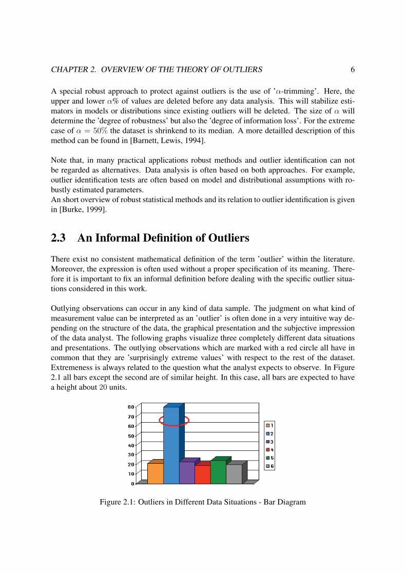
of the data analyst. The following graphs visualize three completely different data situations
and presentations. The outlying observations which are marked with a red circle all have in
common that they are ’surprisingly extreme values’ with respect to the rest of the dataset.
Extremeness is always related to the question what the analyst expects to observe. In Figure
2.1 all bars except the second are of similar height. In this case, all bars are expected to have
a height about 20 units.
Figure 2.1: Outliers in Different Data Situations - Bar Diagram

CHAPTER 2. OVERVIEW OF THE THEORY OF OUTLIERS 7
In Figure 2.2, all data except one value seem to follow a linear model:
Figure 2.2: Outliers in Different Data Situations - Linear Model
The data points in Figure 2.3 may represent a data sample from a normal distributed popula-
tion. Observations accumulate in the middle of the measuring range. Only one isolated value
at the boundary seems suspicious.
Figure 2.3: Outliers in Different Data Situations - Normal Distribution
2.3.1 Outliers, Extreme Values and Contaminants
Outlying observations do not fit with the statistical assumptions which describe the majority
of data. They belong to a different population and thus follow different statistical models or
distributions. In order to describe a dataset which contains observations of several populations,
the following notations will be used for convenience:
Definition 2.1 (Contaminants, Contaminated and Contaminating Population)
Consider a data sample of size N which should be representative for a given population Pint
of interest. Suppose that Ncont < N of the data values correspond to a different population
Pcont �= Pint. Then these Ncont values are called contaminants and the corresponding popu-
lation Pcont is called contaminating population with respect to the contaminated population
Pint. The given data sample thus represents a mixture of the populations Pint and Pcont
rather than Pint.
The mixture of populations will now be defined mathematically:

CHAPTER 2. OVERVIEW OF THE THEORY OF OUTLIERS 8
Definition 2.2 (Mixed Distribution/ Model)
Consider a data sample S of size N which should represent the population Pint and which is
contaminated by the contaminating population Pcont. Suppose that Pint ∼ F and Pcont ∼ Gfor two statistical distributions (or statistical models) F and G with F �= G. Let p be the
probability to choose an observation which belongs to Pint. Then, the data sample S is a
realization of the mixed distribution (or the mixed model)
p · F + (1− p) ·G.
Note that in practical applications p is usually close to 1. The aim is to identify the data which
belongs to the contaminating population Pcont. The problem lays in separating the contami-
nants from the observations of interest. Often this is not entirely possible however.
In general it may be possible that the population of interest Pint is contaminated by several
contaminating populations Pconti for i = 1, ...,m. The separation of several subpopulations is
related to the field of cluster analysis and will not be further discussed here. For the sake of
simplicity, in this work the problem will be reduced to the case of one contaminating popula-
tion Pcont.
To illustrate the problem, consider the case where F and G are two different distributions.
In the following graphical examples, it is assumed that:
F ∼ N(μ1, σ21)
and G ∼ logN(μ2, σ22).
The distributions F and G can be separated best if they differ by a substantial shift of mean.
In the following example, the probability p is given by
p := 0.9
and the distribution parameters are chosen as follows:
μ1 := 3,
μ2 := 7,
σ21 := 1,
σ22 := 1.
Since the contaminating population Pcont has a much higher mean than the population of
interest Pint, observations corresponding to large values are more likely to belong to the con-
taminants than to the population of interest. On the other hand, observations corresponding to
small values are more likely to belong to the population of interest. Note that, contaminants
with a small magnitude will be hidden within the samples which belong to Pint. However, the

CHAPTER 2. OVERVIEW OF THE THEORY OF OUTLIERS 9
probability to observe a contaminant with a small value is very low, so this problem may be
neglected.
Figure 2.4: Mixed Distribution: 0.9 ·N(3, 1) + 0.1 · logN(7, 1)
Separation becomes more difficult if there is no shift in mean but in variance. For
p := 0.9,
choose:
μ1 := 5,
μ2 := 5,
σ21 := 1,
σ22 := 2.
Here, most of the observations of the contaminating and the contaminated population will
have values close to the common mean μ1 = μ2 = 5. Those observations can not adequately

CHAPTER 2. OVERVIEW OF THE THEORY OF OUTLIERS 10
be assigned to one of the populations. Only extreme values with very small or very high
magnitudes are more likely to belong to the contaminants than to the population of interest.
Figure 2.5: Mixed Distribution: 0.9 ·N(5, 1) + 0.1 · logN(5, 2)
It has been shown in examples that contaminants may be identified because of their extreme-
ness. However, they may as well be completely hidden in the population of interest. This fact
will lead to an informal definition of the expression ’outlier’:
Notation 2.3 (Outlier)
An observation of a dataset S will be referred as an outlier, if it belongs to a contaminating
population Pcont and if it is surprisingly extreme with respect to the model or distributional
assumptions for the population of interest Pint.
In practical applications, the true population affiliation of a surprisingly extreme value is usu-

CHAPTER 2. OVERVIEW OF THE THEORY OF OUTLIERS 11
ally not known. Therefore, the following notation is introduced:
Notation 2.4 (Outlier candidate)
An observation of a dataset S will be referred as an outlier candidate, if it is surprisingly ex-
treme with respect to the model or distributional assumptions for the population of interest
Pint.
As the population affiliation usually can not be determined, this work will refer to the term
’outlier candidate’ most of the time. Note that in the literature the above notations are not
consistent.
The expressions ’outlier’ and ’outlier candidate’ can be defined mathematically by fixing a
measure for ’surprisingly extreme’. Usually, this will be done by formulating hypotheses
for an appropriate outlier test. The following remark will give an overview of the relations
between the different notations given in this section:
Remark 2.5
(i.) By the Definitions 2.1, 2.2 and Notation 2.3, outliers are a subset of the contaminants.
(ii.) By Notation 2.3 and 2.4, outliers are a subset of the outlier candidates.
(iii.) Outlier candidates are not necessarily outliers. They may as well correspond to the
population of interest!
(iv.) Contaminants are not necessarily outlier candidates. They can be hidden in the popula-
tion of interest!
Figure 2.6: Population Affiliations
The aim of outlier tests is to separate the true outliers from the population of interest. This can
only be successful if the population of interest Pint is well separated from the contaminating
CHAPTER 2. OVERVIEW OF THE THEORY OF OUTLIERS 12
population Pcont. Most outlier identification rules only test the extremeness of observations
with respect to the distribution of the population of interest Pint without making assumptions
on the contaminating distribution or the mixed model parameter p. This approach was follow
for example by [Davies, Gather, 1993] who defined so called ”‘outlier regions”’ based on the
distributional assumptions for the populations of interest.
Other outlier tests are based on special mixed model assumptions, which is strongly related to
the theory of cluster analysis as mentioned above. Early research on outlier theory with respect
to mixed model assumptions was done by [Dixon, 1950] and [Grubbs, 1950]. They were fol-
lowed by [Anscombe, 1960], [Tukey 1960], [Box, Tiao, 1968], [Guttman, 1973],
[Marks, Rao, 1979], [Aitkin, Wilson, 1980] and many others.
2.3.2 The Diversity of Extremeness
As it has been pointed out in the previous section, a measure for extremeness has to be defined
in order to construct outlier tests and to define the term ’outlier’ mathematically. However, the
question of what should be considered as ’extreme’ is not obvious. In this chapter, the most
important considerations and remarks about extremeness of data values will be concluded.
2.3.2.1 Extremeness with Respect to the Majority of Data
In many data situations extreme observations will correspond to values of very high or very
low magnitude. For most statistical distributions, data points accumulate around the mean
value. Indeed, extreme values do not necessarily correspond to extremely small or big values.
Extremeness is rather correlated to the isolation of the observation.
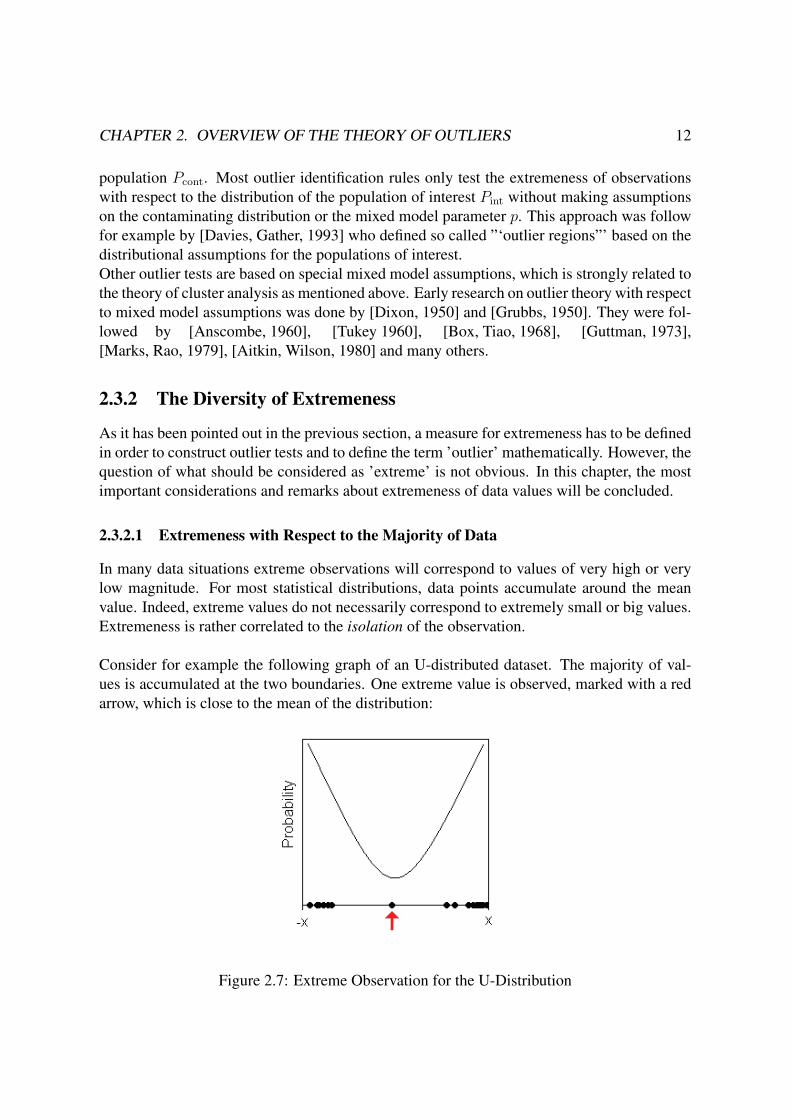
Consider for example the following graph of an U-distributed dataset. The majority of val-
ues is accumulated at the two boundaries. One extreme value is observed, marked with a red
arrow, which is close to the mean of the distribution:
Figure 2.7: Extreme Observation for the U-Distribution

CHAPTER 2. OVERVIEW OF THE THEORY OF OUTLIERS 13
2.3.2.2 The Importance of Underlying Statistical Assumptions
A measure for the extremeness of observations will be determined by the statistical assump-
tions on the dataset. The other way round, wrong statistical assumptions can lead to wrong
conclusions about extreme and non extreme values. For example, surprisingly extreme values
for a normal distribution may not be considered as extreme under a more heavy tailed distri-
bution like Student’s-t.
Wrong assumptions on the data model can cause errors in the interpretation of extreme values
as well. In the following graphical example, the dataset is wrongly assumed to be described
by a linear regression model.
Figure 2.8: Error in the Model Assumption
Several residuals seems extremely high with respect to the regression line. A polynomial of
degree 3 however fit the data almost perfectly and no extreme observation can be identified.
Figure 2.9: Corrected Model Assumption

CHAPTER 2. OVERVIEW OF THE THEORY OF OUTLIERS 14
2.3.2.3 Extremeness in Multivariate Datasets
Extreme values in multivariate datasets are much less obvious to identify than in univariate
datasets. A visual inspection of the dataset is difficult since there often exist no easy way for
a graphical representation. A discussion of this problem can be found in [Buttler, 1996].
A multivariate observations may contain extreme values in the single variables. However,
an extreme value in one variable does not necessarily mean that the corresponding multivari-
ate observation is extreme with respect to the underlying multivariate statistical distribution or
model. The other way round, a multivariate observation may look surprisingly extreme with
respect to the stated distribution or model whereas the values of the single variables all are
just slightly shifted. Consider for example the following three dimensional dataset:
Obs x1 x2 x3
1 4 2 8
2 2 1 4
3 7 1 9
4 1 2 5
5 5 1 7
6 4 12 28
7 3 3 9
8 2 4 2
Table 2.1: Example for a Multivariate Dataset
Here, observation 6 is surprisingly extreme in the variables x2 and x3. However, all data
values expect the 8th observation are perfectly fitted by the two-dimensional regression model
x3 = x1 + 2 · x2. The 8th observation contains no extreme values within the single variables
although it is an obvious outlier candidate:
Figure 2.10: Outlier Candidate from a Two-Dimensional Linear Regression Model

CHAPTER 2. OVERVIEW OF THE THEORY OF OUTLIERS 15
Exemplary methods for the identification of multivariate outliers are discussed in
[Acuna, Rodriguez, 2005].
If several groups of data are compared in a multivariate dataset, outliers can appear with
respect to scale and location measures:
Figure 2.11: Outlier Candidates in Location and in Variance
Group 6 is an outlier candidate in location since the group mean differs significantly from all
other group means. If however the variance of data within a single group is considered, group
4 turns out to be surprisingly extreme.
The principles of scale and location outliers are also discussed in [Burke, 1999]. Examples
for corresponding scale and location outlier tests are given in [Wellmann, Gather, 2003].
2.3.2.4 Ambiguity of Extreme Values
Extreme observations in a dataset may be ambiguous. The following data are described by a
linear regression model. There exist two suspicious observations, marked in blue and green,
but it is not obvious which one of them is an outlier or if maybe both values are outliers.
Figure 2.12: Ambiguity of Extreme Values

CHAPTER 2. OVERVIEW OF THE THEORY OF OUTLIERS 16
The model adjustment is not very satisfying with R2 = 0.825359. If the first or the second
suspicious value is removed, the corresponding linear fit becomes substantial different. As it
can be deduced from the following graphs, both R2 values are much higher now and approxi-
mately of the same magnitude. However, the parameter estimates are very different! Without
further data information, it can not be deduced which observation is spurious or if even both
values are outliers.
Figure 2.13: Linear Fits for Excluded Upper or Lower Extreme Value

CHAPTER 2. OVERVIEW OF THE THEORY OF OUTLIERS 17
If both suspicious values are removed, the fit is given by:
Figure 2.14: Linear Fits with both Extreme Values Excluded
With R2 = 0.995986 the model adjustment has improved a lot. The parameter estimates are
again very different from the previous ones. This points out that the R2-value as a measure of
fit can lead to serious misinterpretations.
2.4 A Short Classification of Outlier Candidates
There exist a variety of different outlier scenarios which differ concerning the structure of the
dataset, the underlying statistical assumptions and the specific interests of the data analyst. It
will be nearly impossible to define detailed subgroups for all possible outlier scenarios within
an overall classification. The aim of this section is to give a classification which points out the
most fundamental differences between the existing outlier scenarios.
As it has been mentioned in Remark 2.5 (iii.), surprisingly extreme values do not always
belong to the contaminating population Pcont. Since in practical application the true popula-
tion affiliation of the extreme value is not known, this section will present a classification for
outlier candidates rather than for true outliers (compare Notation 2.4).
2.4.1 The Statistical Assumptions
In a first classification step the model or distributional assumptions for the population of inter-
est Pint are considered. As it has been mentioned in Section 2.3.2.2, inappropriate statistical
assumptions can lead to wrong conclusion on outlier candidates. Therefore, it should be veri-
fied if the outlier candidate is judged with respect to the right statistical assumptions.

CHAPTER 2. OVERVIEW OF THE THEORY OF OUTLIERS 18
2.4.2 Causes for Extreme Values
In the second classification step, outlier candidates will be divided into outliers, which belong
to the contaminating population Pcont and extreme observations which are valid members of
the population of interest Pint. In other words, the outlier candidates are classified concerning
the cause for their extremeness. True outliers are due to the fact that the population of interest
Pint really is contaminated. Extreme values which do not belong to the contaminants are due
to the natural variance in the population of interest Pint. In this case, the outlier candidate
provides a part valid information on the population of interest.
2.4.3 Different Goals of Outlier Identification
The last step in the classification of outliers will be determined by the predefined goal for the
outlier identification, which will influence the formulation of hypothesis for the outlier test.
If the outlier candidate is due to an error in the statistical assumptions for the population of
interest, the aim will be to adjust these assumptions. After an appropriate adjustment of the
statistical model, the outlier candidate becomes a regular member of the population of inter-
est. If the outlier candidate really is a contaminant, the causes for the contamination should
be explored and removed whenever possible. A new measurement under corrected conditions
can replace the outlying value. Care have to be taken with the identification of contamination
causes since identifying wrong causes may effect the results of data analysis. If the outlier
candidates belongs to the population of interest it should not be removed since they involve
valid information about the underlying distribution.
In most cases however, it is not easy or even impossible to decide whether an outlier candidate
is due to the natural variation in the population of interest or if it is due to contamination or if
it reflects a misconception in the statistical modeling.
A supplementary possibility to deal with outlier candidates which will not be further dis-
cussed here is ’accommodation ’ as referred in [Barnett, Lewis, 1994]. This can be done by
’Winsorization’ where outlier candidates are replaced by their nearest neighbors.
The following flow chart will visualize the different steps of outlier classification.

CHAPTER 2. OVERVIEW OF THE THEORY OF OUTLIERS 19
Figure 2.15: Classification of Outlier Candidates

Chapter 3
Different Concepts for Outlier Tests
The identification of outlier candidates as motivated in Chapter 2 will be based on statistical
tests. Thereby, the diversity of outlier scenarios correspond to a broad field of different outlier
tests. In this chapter, several types of outlier test will be presented. In Section 3.1, a short
classification of different outlier tests will be given whereas Section 3.2 describes different
types of test hypotheses. Finally, in Section 3.3, some basic problems which can be met in the
identification of outliers are presented.
With the notations introduced in Section 2.3.1, the term ’outlier test’ is misleading. Since
the true population affiliation of an outlier candidate is not known, it would be more conve-
nient to talk about ’tests to identify outlier candidates’. The term ’outlier candidate’ is the
more appropriate in hardly any practical context. For the sake of simplicity however, the term
’outlier’ will be used in general for the remainder of this work. It will be clear from the
context, if the true population affiliation is known or not.
3.1 Classification of Outlier Tests
There exists several types of outlier tests. Some tests only check a predefined number of
suspicious extreme values. Other tests scan the whole dataset for outlying measurements
without selecting suspicious candidates in advance. In the following sections, these concepts
will be further explained and exemplary tests will be presented.
3.1.1 Tests for a Fixed Number of Outlier Candidates
In many practical applications, the user identifies one or a few suspicious values within the
dataset based on his subjective impression and his experience in the field. Hence, he wishes
to test a fixed number of predefined outlier candidates. A corresponding outlier test for one
suspicious value will be based on the following informal hypotheses:
20

CHAPTER 3. DIFFERENT CONCEPTS FOR OUTLIER TESTS 21
H0 : The suspicious value is no true outlier and thus belongs to Pint,
versus
H1 : The suspicious value really is an outliers and belongs to Pcont.
Equivalent hypotheses will be formulated if several predefined outlier candidates are to be
tested:
H0 : At least one of the suspicious values belongs to Pint,
versus
H1 : All suspicious values belong to Pcont.
Note that an outlier test based on the above hypotheses do not provide a global answer with
regard to the presence or absence of any outliers. Therefore, this kind of test is only appropri-
ate if the data analyst who decides which values seem suspicious is well experienced with the
type of data situation.
Many stepwise procedures for the identification of outliers have been proposed in this context,
compare for example [Hawkins, 1980] (Chapter 5, Pages 63-66). An exemplary outlier test
for one predefined extreme value is the well known Grubb’s Test [Grubbs, 1950]. Here, the
absolute difference between the mean value of data and the outlier candidate divided by the
standard deviation is compared to predefined distributional quantiles. Other examples can be
found in [Hawkins, 1980] (Chapter 3, Pages 27-40 and Chapter 5, Pages 52-67).
3.1.2 Tests to Check the Whole Dataset
As it has been explored in Section 2.3.2, it is not always obvious which values are extreme
realizations with respect to the underlying statistical distribution or model. Therefore out-
lier candidates may be hard to distinguish. Hence, an outlier test is needed which scans the
whole dataset for the presence of any outlier. In this case, hypotheses will be stated as follows:

CHAPTER 3. DIFFERENT CONCEPTS FOR OUTLIER TESTS 22
H0 : The dataset does not contain any outlier,
versus (3.1.1)
H1 : There are outliers present in the dataset.
Usually, the outlier test should not only be able to state the presence of outliers but to identify
them, as well. Therefore, most global outlier test are constructed by calculating predefined
outlier limits, which are given in form of confidence limits for the specific comparison mea-
sure. Test decision is made by comparing the measure of interest to the particular outlier
limits. H0 is rejected if any of the measurement values exceeds the given outlier limits. All
measurement values which lay outside the predefined outlier limits are identified as outlier.
For a dataset of sample size n, the global test (3.1.1) is thus given as a multiple test situation
consisting of n single tests. For i = 1, ..., n the hypotheses for these single tests are given by:
Hi,0 : The ith measurement value is no outlier,
versus (3.1.2)
Hi,1 : The ith measurement value is an outlier.
As (3.1.1) is a multiple test situation, this will lead to the accumulation of first order errors.
Therefore, the local significance levels αloc for the single tests (3.1.2) should be adjusted in
order to keep a global significance level αglob.
The most common method to adjust the local significance levels is the well known Bonferroni
adjustment, compare [Hsu, 1996] (Chapter 1, Page 13):
αloc =αglob
n.
The method of Bonferroni is the simplest and most flexible adjustment procedure proposed
in the literature. It can be used in any multiple testing situation, requires no further statistical
assumptions and is simple and fast to calculate. Unfortunately, it may lead to a notable loss
of power - especially for a high number of strongly correlated tests. Therefore, an outlier test
based on the Bonferroni adjustment should always be accompanied by a visual inspection of
the data.
A less conservative alternative which however requires more computational effort is the step-
wise Bonferroni-Holmes procedure proposed by [Holm, 1979]. However, there exist many
other methods to adjust the local significance levels in a multiple testing situation. An

CHAPTER 3. DIFFERENT CONCEPTS FOR OUTLIER TESTS 23
overview of the different procedures is given in [Hochberg, Tamhane, 1987] and [Hsu, 1996].
The adjustment procedures differ with respect to the power loss, the underlying computational
effort and the required statistical assumptions.
As the focus of the outlier test lays not exclusively on the global test hypotheses (3.1.1) but
also on the local test hypotheses (3.1.2), this will lead to extended performance measures for
the statistical test. For the test (3.1.1), the power is defined as the probability to detect outliers
under the condition that the dataset truly contains outliers. This does not imply that the test
identifies the right observations as outliers. The probability to identify the right observations
as outliers under the condition that the dataset contains outliers will be a supplementary mea-
sure of performance. These performance measures are discussed by [Hawkins, 2002] (Chapter
2, Pages 13-14).
The LORELIA Residual Test developed in the context of this work is an example for an
outlier test which scans the whole dataset for outlying measurements. Other examples can be
found in [Davies, Gather, 1993] and [Hawkins, 2002] (Chapter 5, Pages 57-63).
3.2 Formulation of the Test Hypotheses
The formulation of the test hypotheses is highly related to the predefined goal of outlier iden-
tification which allows to classify them in different subgroups.
3.2.1 Discordancy Tests
If the goal of outlier identification is to eliminate the existing outliers, the task is to separate
the contaminating population Pcont from the population of interest Pint and to exclude outliers
before any further data analysis. Test hypotheses for a corresponding outlier test will be for-
mulated as follows:
H0 : All observations fit with the given statistical assumptions for Pint,
versus
H1 : There exist observations which are discordant to the given
statistical assumption of Pint.
Tests with the above hypotheses will be referred as ’discordancy tests’ as stated in
[Barnett, Lewis, 1994] (Chapter 2, Pages 37-38).

CHAPTER 3. DIFFERENT CONCEPTS FOR OUTLIER TESTS 24
3.2.2 Incorporation of Outliers
If there exist observations which do not fit with the stated model or distributional assumptions
for Pint, it may be appropriate not to eliminate these values but to explain them by supple-
mentary or new assumptions. In [Barnett, Lewis, 1994] (Chapter 2, Page 39) this is referred
as ’incorporation of outliers’. There exist several ways to incorporate outliers which will be
presented in the following sections.
3.2.2.1 The Inherent Hypotheses
As it has been explained in Section 2.4.2, extremeness of measurement values may be due to
wrong model assumptions for the population of interest. Test hypotheses should thus state an
alternative model or distribution for the whole dataset:
H0 : All data are explained well by the given model or distribution,
versus
H1 : All data are explained better by another predefined model or
distribution.
Since test based on these hypotheses are based on the assumption that the whole dataset be-
longs to the same population, they are referred as ’inherent hypotheses’ in
[Barnett, Lewis, 1994] (Chapter 2, Page 46). The alternative model or distribution stated in
H1 may differ only by a change of the parameters but it may as well be a completely different
model or distribution.
3.2.2.2 The Deterministic Hypotheses
Instead of adjusting the statistical assumptions for the whole dataset, hypotheses may state an
alternative model or distribution for the suspicious values only:
H0 : All data are explained well by the given model or distribution,
versus
H1 : Some suspicious values are explained better by another predefined
model or distribution.

CHAPTER 3. DIFFERENT CONCEPTS FOR OUTLIER TESTS 25
In [Barnett, Lewis, 1994] (Chapter 2, Page 45), these hypotheses are called ’deterministic’.
The deterministic alternative is closely related to the ’mixed model alternative’ which will be
presented in the following.
3.2.2.3 The Mixed Model Alternative
Mixed models and distributions have been defined in Definition 2.2 in Section 2.3.1. In the
case of existing extreme observations, an alternative mixed model or distribution is stated,
which explains the outlying values as well as the normal data. Hypotheses are given as fol-
lows:
H0 : All data are explained well by the given model or distribution,
versus
H1 : Most observations are well explained by the given assumptions
but with a small probability 1− p the observations follow another
model or distribution.
The problem here is to estimate the distribution parameters for the mixed model as parameter
estimates for the contaminating distribution or model are usually based on very few data
points.
3.3 Problems and Test Limitations
In this Section some problems which may lead to incorrect outlier classifications are pointed
out.
3.3.1 The Masking Effect
The presence of several outliers in a dataset may avoid the identification of even one outlier.
This is called the ’masking effect’. To illustrate this, consider a common outlier test in which
the outlier candidate is compared to its right or left neighbor respectively. A big difference
indicate that the outlier candidate is isolated and hence really is a true outlier. A small differ-
ence is expected to indicate that the measurement value is not isolated. However, if several
outliers lay close together, this may lead to a masking effect.
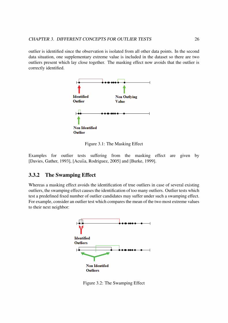
In the following graphic, two data situations are presented. In the first data situation, one
CHAPTER 3. DIFFERENT CONCEPTS FOR OUTLIER TESTS 26
outlier is identified since the observation is isolated from all other data points. In the second
data situation, one supplementary extreme value is included in the dataset so there are two
outliers present which lay close together. The masking effect now avoids that the outlier is
correctly identified.
Figure 3.1: The Masking Effect
Examples for outlier tests suffering from the masking effect are given by
[Davies, Gather, 1993], [Acuna, Rodriguez, 2005] and [Burke, 1999].
3.3.2 The Swamping Effect
Whereas a masking effect avoids the identification of true outliers in case of several existing
outliers, the swamping effect causes the identification of too many outliers. Outlier tests which
test a predefined fixed number of outlier candidates may suffer under such a swamping effect.
For example, consider an outlier test which compares the mean of the two most extreme values
to their next neighbor:
Figure 3.2: The Swamping Effect
CHAPTER 3. DIFFERENT CONCEPTS FOR OUTLIER TESTS 27
In the first data situation, the two outliers are correctly identified since their mean is far away
from the main body of the data. In the second data situation, only one true outlier exists. The
mean between the outlier and its next neighbor however is still very large compared to the
values of the remaining dataset. Thus, both values will be classified as outliers by this test.
Examples for the swamping effect are discussed in [Davies, Gather, 1993] and
[Acuna, Rodriguez, 2005].
3.3.3 The Leverage Effect
The estimation of non robust linear regression parameters can be influenced substantially by
so called ’leverage points’. Leverage points are measurement values at the edge of the mea-
suring range which are isolated to the main body of the data. Varying values of leverage points
lead to very different parameter estimates and thus influence the identification of outliers.
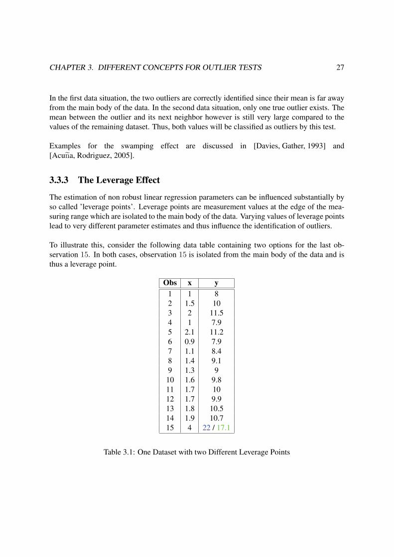
To illustrate this, consider the following data table containing two options for the last ob-
servation 15. In both cases, observation 15 is isolated from the main body of the data and is
thus a leverage point.
Obs x y1 1 8
2 1.5 10
3 2 11.5
4 1 7.9
5 2.1 11.2
6 0.9 7.9
7 1.1 8.4
8 1.4 9.1
9 1.3 9
10 1.6 9.8
11 1.7 10
12 1.7 9.9
13 1.8 10.5
14 1.9 10.7
15 4 22 / 17.1
Table 3.1: One Dataset with two Different Leverage Points

CHAPTER 3. DIFFERENT CONCEPTS FOR OUTLIER TESTS 28
A simple linear regression fit for the first dataset delivers the following results:
Figure 3.3: Linear Regression with the First Leverage Point Included
With R2 = 0.961292 the linear model seems highly appropriate for the given dataset. Now,
consider the linear regression fit with the second leverage point included:
Figure 3.4: Linear Regression with the Second Leverage Point Included
With R2 = 0.991788 the model adjustment has improved a lot. The parameter estimates are
very different from those of the first dataset. The influence of the leverage point is obvious.
In practical applications, parameter estimates which may suffer from a leverage effect must
always be handled and interpreted with care. Leverage points may bias the estimates but they
can as well stabilize them. Therefore, a supplementary data analysis without the leverage
point may be helpful. Thus, consider the regression fit with both leverage points excluded:

CHAPTER 3. DIFFERENT CONCEPTS FOR OUTLIER TESTS 29
Figure 3.5: Linear Regression without the Leverage Points
Here R2 = 0.968896, so the model adjustment is superior to the one with the first leverage
point included, but inferior to the one with the second leverage point included. Moreover,
the parameter estimates are very similar to those for the second dataset. Hence, the second
leverage point stabilize the parameter estimates, whereas the first bias them. A discussion on
leverage points and how to deal with them is given in [Rousseeuw, Zomeren, 1990].

Chapter 4
Evaluation of Method ComparisonStudies
Method comparison studies are performed to evaluate the relationship between two measure-
ment series. In clinical chemistry, they may for example be conducted to compare two mea-
surement methods, two instruments or two diagnostic tests. Often the aim is to compare the
performance of a newly developed method to a well established reference method. Several
samples at different concentration levels are measured with both methods or instruments, re-
spectively. These measurement tuple series are compared in order to show the equivalence
between the two methods or to detect systematic differences.
There exist several possibilities to evaluate method comparison studies. A common approach,
which is presented in Section 4.1, is to calculate the differences between two corresponding
measurement values and to analyze these differences. Another possibility to compare two
measurement series, which is discussed in Section 4.2, is the fit of a linear regression line.
Both approaches require special distributional assumptions, which are not always met for the
original data, but may be fulfilled after an appropriate data transformation, for example a log
transformation or a generalized log transformation, compare [Rocke, Lorenzato, 1995]. A
general overview of the different evaluation procedures and possible data transformations is
given by [Hawkins, 2002]. The different measurement error models used in this context are
summarized in the work of [Cheng, Ness, 1999].
4.1 Comparison by the Method Differences
In order to compare two measurement series, it is a common practice to determine the dif-
ferences between the corresponding x- and y-values and to compare its average and standard
deviation to some predefined limits to test equivalence. There exists several alternatives to
calculate the differences.
30

CHAPTER 4. EVALUATION OF METHOD COMPARISON STUDIES 31
4.1.1 The Absolute Differences
One common procedure is discussed by [Altman, Bland, 1983], [Bland, Altman, 1986],
[Bland, Altman, 1995] and [Bland, Altman, 1999] which propose to use the absolute differ-
ences.
For n ∈ N, let x1, ..., xn and y1, ..., yn be two measurement series corresponding to method
Mx and My respectively. The observed measurement values are assumed to be described by:
xi = ci + αx + εx (4.1.1)
yi = ci + αy + εy, for αx, αy ∈ R, i = 1, ..., n, (4.1.2)
where ci is the unbiased, true concentration which is biased by the systematic additive term
αx respective αy and the measurement error εx respective εy. The measurement errors εx and
εy are realizations of the random variables:
Ex ∼ N(0, σ2x), (4.1.3)
Ey ∼ N(0, σ2y). (4.1.4)
The absolute differences, which are given by:
dabsi := yi − xi, i = 1, ..., n (4.1.5)
are therefore realizations of the random variable:
Dabsi = αy − αx + Ey − Ex
∼ N(αy − αx, σ2x + σ2
y),
=: N(μdabs, σ2
dabs). (4.1.6)
Now, calculate the 97.5% confidence limits for the absolute differences Dabs:
dabs ± z97.5% · Sdabsdabs , (4.1.7)
where z97.5% is the corresponding quantile of the normal distribution, dabs
is the mean and
Sdabsdabs is the empirical standard deviation of dabs1 , ..., dabs
n . In [Bland, Altman, 1986], these
confidence limits are called the ’limits of agreement’. In order to test equivalence between the
two methods, the limits of agreement are compared to predefined clinical reference values.
Confidence bounds for the limits of agreement can be calculated as described by
[Bland, Altman, 1986] and [Bland, Altman, 1999] in order to estimate the influence of the
sampling error. Note that these limits of agreement are not robust against outliers since they
are based on non robust location and scale estimators. Thus, the dataset should be checked for
outliers in advance (compare Section 5.1).
Assumption (4.1.6) can be visually verified with the help of a scatter plot where the abso-
lute differences dabsi are plotted against the means of the measurement values xi+yi
2.

CHAPTER 4. EVALUATION OF METHOD COMPARISON STUDIES 32
Figure 4.1: Method Comparison based on the Absolute Differences
The mean values xi+yi
2are distributed as follows:
1
2(Xi + Yi) ∼ N
(ci +
1
2(αx + αy),
1
4(σ2
x + σ2y)
), for i = 1, ..., n. (4.1.8)
Thus, the mean values xi+yi
2are only unbiased estimators for the true concentration ci if:
αx = αy = 0. (4.1.9)
However, even if (4.1.9) is not fulfilled, the visual inspection of the scatter plot is still ap-
propriate since a systematical bias on the horizontal axis will not affect the general normal
assumption (4.1.6).
4.1.2 The Relative Differences
In many practical applications, the absolute differences will not have constant mean and vari-
ance over the measuring range. If the scatter plot reveals a proportional difference between
measurement values, it will be more appropriate to consider a multiplicative random error.

CHAPTER 4. EVALUATION OF METHOD COMPARISON STUDIES 33
Figure 4.2: Proportional Bias Between Methods
The following model assumptions are considered:
xi = ci · βx + εxi(4.1.10)
yi = ci · βy + εyi, for βx, βy ∈ R
+, i = 1, ..., n, (4.1.11)
where the random errors are realizations of the random variables:
Exi∼ N(0, c2
i · σ2x), (4.1.12)
Eyi∼ N(0, c2
i · σ2y), for i = 1, ..., n. (4.1.13)
Note that the error variances in (4.1.12) and (4.1.13) depend on the true concentrations ci.
The absolute differences are thus realizations of:
Dabsi = ci · (βy − βx) + Eyi
− Exi
∼ ci ·N(βy − βx, σ2x + σ2
y), for i = 1, ..., n. (4.1.14)
The variance and the mean of the absolute differences are not constant here, but increase
proportionally in ci. By (4.1.14), this corresponds to the assumption of a constant coefficient
of variance for th random errors. Note that the true concentrations ci are not known here!
They therefore have to be estimated, which is done by the mean of the observed measurement
values:
ci =yi + xi
2, for i = 1, ..., n. (4.1.15)
The mean values are distributed as follows:
1
2(Xi + Yi) ∼ N
(ci
2(βx + βy),
c2i
4(σ2
x + σ2y)
), for i = 1, ..., n. (4.1.16)

CHAPTER 4. EVALUATION OF METHOD COMPARISON STUDIES 34
Again, the mean values xi+yi
2are only unbiased estimators for the true concentration ci if:
βx = βy = 1. (4.1.17)
The normalized relative differences are defined by:
dnormreli :=
yi − xi
12· (yi + xi)
, for i = 1, ..., n. (4.1.18)
If the mean xi+yi
2is chosen as an estimate for the true concentration ci, they are approximately
distributed as:
Dnormreli
approx∼ 2
(βx + βy)·N(βy − βx, σ
2x + σ2
y),
=: N(μdnormrel, σ2
dnormrel). (4.1.19)
The normalized relative differences have constant mean and variance. Hence the limits of
agreement can be calculated as the 97.5% confidence limits:
dnormrel ± 1.96 · Sdnormreldnormrel , (4.1.20)
where dnormrel
is the mean and Sdnormreldnormrel is the empirical standard deviation of
dnormrel1 , ..., dnormrel
n .
Figure 4.3: Method Comparison based on the Normalized Relative Differences

CHAPTER 4. EVALUATION OF METHOD COMPARISON STUDIES 35
The dataset for the above scatter plot is the same as in Figure 4.2. Whereas Figure 4.2
clearly shows that the absolute differences are not normally distributed, the normal assump-
tions seems appropriate for the normalized relative differences plotted in Figure 4.3.
In the literature, the special case that one method (here Mx) is free of random error is of-
ten considered, as well. This correspond to the following model assumptions:
xi = ci (4.1.21)
yi = ci · βy + εyi, for βy ∈ R
+, i = 1, ..., n, (4.1.22)
with εy being a realization of the random variable:
Eyi∼ N(0, c2
i · σ2y), for i = 1, ..., n. (4.1.23)
In this case, the absolute differences have the following distribution:
Dabsi = ci · (βy − 1) + Eyi
∼ ci ·N(βy − 1, σ2y), for i = 1, ..., n. (4.1.24)
Since method Mx is free of random error, the true concentration ci is known here and does not
have to be estimated. Therefore, the relative differences can be considered:
dreli :=
yi − xi
xi
, for i = 1, ..., n, (4.1.25)
which are realizations of:
Drel ∼ N(βy − 1, σ2y),
=: N(μdrel, σ2
drel). (4.1.26)
Again the limits of agreement can be calculated as the 97.5% confidence limits:
drel ± 1.96 · Sdreldrel , (4.1.27)
where drel
is the mean and Sdreldrel is the empirical standard deviation of drel1 , ..., drel
n . Assump-
tion (4.1.26) can be verified by plotting xi against the relative differences yi−xi
xi.

CHAPTER 4. EVALUATION OF METHOD COMPARISON STUDIES 36
Figure 4.4: Method Comparison based on the Relative Differences
4.2 Comparison with Regression Analysis
The statistical comparison of two measurement series is often evaluated by fitting a linear re-
gression line. The outcomes of the two methods which are to be compared are plotted against
each other and a regression line is calculated. The evaluation of method comparison studies
by regression analysis is discussed in [Hartmann et al. 1996].
Consider the following model assumptions as described by [Fuller, 1987] (Chapter I, Page
1):
xi = αx + βx · ci︸ ︷︷ ︸=:xi
+ εxi(4.2.1)
yi = αy + βy · ci︸ ︷︷ ︸=:yi
+ εyi, for i = 1, ..., n, (4.2.2)
where ci is the true concentration and xi, yi are the expected measurement values for method
Mx and My respectively which are exposed to the measurement errors εxiand εyi
. Without
loss of generality it will be assumed that:
xi = ci + εxi(4.2.3)
yi = α+ β · ci + εyi, for i = 1, ..., n. (4.2.4)

CHAPTER 4. EVALUATION OF METHOD COMPARISON STUDIES 37
The measurement errors εxiand εyi
are assumed to be realizations of the random variables:
Exi∼ N(0, σ2
xi), (4.2.5)
Eyi∼ N(0, σ2
yi), for i = 1, ..., n. (4.2.6)
The observed measurement values are hence realizations of the random variables:
Xi = xi + Exi∼ N(xi, σ
2xi) (4.2.7)
Yi = yi + Eyi∼ N(yi, σ
2yi), for i = 1, ..., n. (4.2.8)
By (4.2.1) to (4.2.4), a linear relationship between the expected measurement values is as-
sumed:
yi = α+ β · ci = α+ β · xi, for α ∈ R, β ∈ R\ {0} , i = 1, ..., n. (4.2.9)
Since the expected measurement values are not known, α and β have to be estimated by re-
gression procedures.
For equivalent methods Mx and My the parameter estimates will be given by:
β ≈ 1,
α ≈ 0.
A proportional bias between the two methods will be given if
β �= 1.
Note that by assumptions (4.2.1) and (4.2.2) the regression method has to take random errors
in both axes into account. Therefore ordinary least square regression is not appropriate in this
context.
There exists a variety of robust and non robust regression methods. Since outlying mea-
surements can effect the estimates of slope and intercept for non robust regression, the recom-
mendation is to use robust regression procedures. Common robust regression methods will be
presented and discussed in the following section.
4.2.1 Robust Regression Methods
There exist a variety of robust regression methods which are based on different statistical
assumptions.An overview can be found in [Rousseeuw, Leroy, 1987]. The procedure recom-
mended in this work is Passing-Bablok regression, which will be presented in the following.
In the literature, principal component analysis and standardized principal component analysis
are often referred as robust procedures as well, although they are parametric. Both meth-
ods are special cases of the more general Deming regression described in [Deming, 1943]
CHAPTER 4. EVALUATION OF METHOD COMPARISON STUDIES 38
and [Linnet, 1998]. Deming regression is the most commonly used procedure in the con-
text of method comparison studies and will therefore be presented in this section as well,
although it can not be regarded as a robust procedure. A comparison and a detailed discussion
of the above regression methods can be found in [Stokl et al., 1998]. Other robust regres-
sion methods are proposed by [Brown, 1988], [Feldmann, 1992], [Ukkelberg, Borgen, 1993],
[Hartmann et al. 1997] and [Olive, 2005]. The following sections are basically referred to the
work of [Haeckel,1993] (Chapter 11, Pages 212-226).
4.2.1.1 Deming Regression
For the Deming regression, the measurement errors εxiand εyi
are assumed to be realizations
of the random variables:
Exi∼ N(0, σ2
x), (4.2.10)
Eyi∼ N(0, σ2
y), for i = 1, ..., n. (4.2.11)
Note, that the error variances are assumed to remain constant over the measuring range here.
Further, a known ratio of error variances is assumed:
σ2y
σ2x
= η2, for a known η ∈ R+\ {0} . (4.2.12)
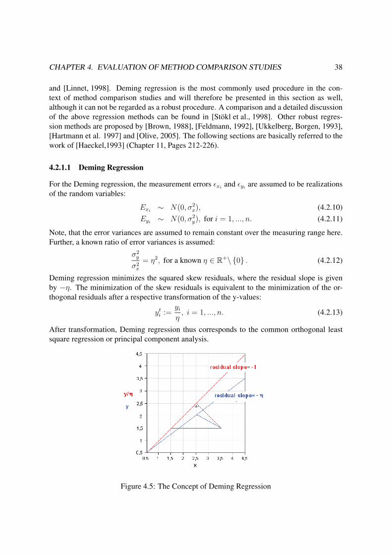
Deming regression minimizes the squared skew residuals, where the residual slope is given
by −η. The minimization of the skew residuals is equivalent to the minimization of the or-
thogonal residuals after a respective transformation of the y-values:
yti :=
yi
η, i = 1, ..., n. (4.2.13)
After transformation, Deming regression thus corresponds to the common orthogonal least
square regression or principal component analysis.
Figure 4.5: The Concept of Deming Regression

CHAPTER 4. EVALUATION OF METHOD COMPARISON STUDIES 39
In the above plot, the blue line corresponds to the regression line for the original measurement
values with skew residuals. The red line shows the regression line after the transformation of
the y-values. The residuals are orthogonal now.
4.2.1.2 Principal Component Analysis (PCA)
Regression analysis by principal component decomposition is equivalent to orthogonal least
square regression. It is a special case of the more general Deming regression described in the
previous section. For a multivariate dataset the principal components are chosen iteratively.
The first principal component is the vector with the direction of the highest variance in data
dispersion. The other principal components are chosen in the same way with the restriction
to be orthogonal to each other. For a two dimensional dataset, this is equivalent to orthogonal
least square regression. PCA is based on the assumption, that the measurement errors are
distributed as follows:
Exi, Eyi
iid∼ N(0, σ2), for i = 1, ..., n, (4.2.14)
which correspond to the special case of equal error variances in (4.2.5) and (4.2.6) or an error
variance ration of η = 1 in (4.2.12).
The slope estimator for principal component analysis is given as:
βPCA :=S2
yy + S2xx +
√(S2
yy − S2xx
)2+ 4 · S2
yx
2 · Syx
, (4.2.15)
where Sxx and Syy are the empirical standard deviations of the x- and y−values, respectively
and S2yx is the corresponding empirical covariance. The estimator for the intercept is defined
through:
αPCA := y − βPCA · x. (4.2.16)
As the orthogonal residuals are always smaller or equal to the vertical residuals, outlying
measurements will intuitively influence the parameter estimates for orthogonal regression less
than for ordinary least square regression. Nevertheless, the PCA can not be regarded as an
outlier resistant regression method since it is still based on non robust parameter estimators.
4.2.1.3 Standardized Principal Component Analysis (SPCA)
Standardized principal component analysis is a special case of Deming regression, as well.
Here, the error variance ratio is assumed to be given by:
σ2y
σ2x
= β2, (4.2.17)

CHAPTER 4. EVALUATION OF METHOD COMPARISON STUDIES 40
where β is the true slope given in (4.2.4). The above functional relationship between the true
slope β and the error variances is assumed in order to reduce the parameters which has to be
estimated. By (4.2.17), the random errors are realizations of:
Exi
iid∼ N(0, σ2x), (4.2.18)
Eyi
iid∼ N(0, β2 · σ2x︸ ︷︷ ︸
=:σ2y
), for i = 1, ..., n. (4.2.19)
Note that (4.2.19) correspond to the assumption that:
yi = α+ β · ci +N(0, β2 · σ2x), for i = 1, ..., n. (4.2.20)
For α = 0 this is equivalent to the error model for the (normalized) relative differences given
in (4.1.11) and (4.1.22).
If βSPCA is the slope of the first principal component, the second component in SPCA will
correspond to a slope of−βSPCA. Note that the slope of the second component determines the
slope of the residuals, as well. The regression parameter estimators are given as:
βSPCA := sign(Syx) ·√
S2yy
S2xx
(4.2.21)
and
αPCA := y − βPCA · x. (4.2.22)
Note, that the use of SPCA is only appropriate if assumption (4.2.20) is fulfilled. A propor-
tional bias between methods can be visually detected with the help of a scatter plot as given
in Figure 4.2.
A geometrical interpretation of PCA and SPCA is given in Figure 4.6:
Figure 4.6: Residuals for PCA and SPCA

CHAPTER 4. EVALUATION OF METHOD COMPARISON STUDIES 41
4.2.1.4 Passing-Bablok Regression
Passing-Bablok regression requires the least strong statistical assumptions among the pre-
sented regression procedures. The following model assumptions have to be fulfilled:
• The random errors Exiand Eyi
of method Mx respective My come from the same type
of an arbitrary continuous distribution. Note that this is a much weaker assumption than
stated in (4.2.5) and (4.2.6).
• The error variances may depend on the true concentration ci, so they are not required to
be constant over the measuring range, as required for Deming regression, but they have
to remain proportional:
σ2yi
σ2xi
= η2, for η ∈ R+\ {0} , i = 1, ..., n. (4.2.23)
Note that the parameter η does not have to be known here!
• The true slope defined by (4.2.9) is close to 1:
β ≈ 1. (4.2.24)
Passing-Bablok regression as described in [Passing, Bablok, 1983], [Passing, Bablok, 1984]
and [Bablok et al. 1988] is based on the concept of Theil’s regression [Theil 1950]:
In a first step, the slopes of the straight lines between all possible data pairs are calculated:
Sij :=
⎧⎪⎪⎪⎪⎨⎪⎪⎪⎪⎩yi−yj
xi−xj, for xi �= xj and yi �= yj,
∞, for xi = xj and yi < yj,
−∞, for xi = xj and yi > yj,
0, for yi = yj,
for all i, j = 1, ..., n.
Without loss of generality, it will be assumed that:
|Sij| ∈ R\ {0} , for all i, j = 1, ..., n.
This is appropriate, since (X, Y ) is a continuous bivariate random variable and hence the
probability to observe values with Sij = 0 or |Sij| = ∞ equals 0. Now, consider the ranked
sequence S(1) ≤ S(2) ≤ ... ≤ S(n).
In [Theil 1950], the median of the above sequence is defined as the slope estimator. Note
however, that the Sij are not statistically independent. Hence, a simple median estimator may
be biased. A bias correction is proposed in [Passing, Bablok, 1983] by the following offset:
K := # {Sij : Sij < −1, for i, j = 1, ..., n} . (4.2.25)

CHAPTER 4. EVALUATION OF METHOD COMPARISON STUDIES 42
The corrected median estimator is given as:
βPB :=
⎧⎨⎩S(N+12
+K), if n is odd,
12·(S(N
2+K) + S(N
2+1+K)
), if n is even.
(4.2.26)
In ([Passing, Bablok, 1984], page 717) it is proved that this slope estimator is independent
of the assignment of the methods to x and y. Moreover it is shown empirically that βPB is
an unbiased slope estimator if the true relation between method Mx and My correspond to a
slope of 1.The estimator for for the intercept is defined as:
αPB := med{1≤i≤n}(yi − β · xi).
Since the error variances remain proportional over the measuring range by assumption (4.2.23)
and the true slope β is assumed to be close to 1, it will be appropriate to consider the orthog-onal residuals in order to describe the location of the data pairs (xi, yi) with respect to the
Passing-Bablok regression line.
Note that as a non parametric method Passing-Bablok regression is more robust against out-
liers than PCA or SPCA.

Chapter 5
Common Outlier Tests for MethodComparison Studies
The presence of outliers in method comparison studies can influence statistical data analy-
sis and hence may lead to wrong conclusions on equivalence or non equivalence for the two
methods. This can basically be avoided by using robust statistical methods, which are resis-
tant against the presence of a few outliers.
However, the identification of outliers is still a very important task if method comparison
is based on robust statistical methods, since the presence of outliers can reveal valuable infor-
mation on the measurement process. Outliers can indicate
• a lack of performance in one of the two methods. For example, a newly developed
method may work equally good as the reference method for samples at the lower con-
centration range, but fails for higher concentrated samples.
• a problem with the specific sample. For example, a somehow contaminated sample may
lead to unexpectedly large measurement values.
For the above reasons, identified outliers should always be carefully examined and reported.
Many different outlier test are described in the statistical literature. A general overview can
be found in [Hawkins, 1980] and [Barnett, Lewis, 1994]. Most outlier tests are constructed to
test a predefined number of extreme values, compare Section 3.1.1. From a visual inspection
of the dataset however, it is not always obvious which values can be regarded as extreme. For
example, typical datasets in method comparison studies often show a very inhomogeneous
sample distribution - the main part of the data is accumulated at a low concentration range
(sample results from the healthy part of the study population) whereas only some isolated
values correspond to higher concentrated samples (sample results from the pathological part
of the population). An outlier classification for isolated values is generally difficult, even if
the corresponding values seem surprisingly extreme, as the local level of data evidence is very
43

CHAPTER 5. COMMON OUTLIER TESTS FOR MCS 44
low. The other way round, extreme values may not be visually detected, if the graphical rep-
resentation is inappropriate. Therefore, it is strongly recommended to scan the whole dataset
for the presence of outliers, as described in Section 3.1.2. Unfortunately, the statistical litera-
ture offers very few suggestions how to deal with the special problem of a unknown number
of outliers most of which require that the measurement values can be ranked with respect to
their extremeness, compare for example [Hawkins, 1980] (Chapter 5, Pages 51-73). However,
as a ranking for the extremeness of measurement values is often note possible as described
above, these procedures are not appropriate in this context. Another intuitive approach which
is followed by [Wadsworth, 1990] is to calculate predefined outlier limits, which are given
in form of robust confidence limits for the specific comparison measure. This concept is
closely related to the informal identification of outliers with the help of boxplots. Although
the test proposed by [Wadsworth, 1990] is not very established in the statistical literature as
it provides no proper type 1 error control, it is a simple solution to handle the special outlier
problem described above and will therefore be used as the reference method in the context of
this work.
5.1 Outlier Tests based on Method Differences
If method comparison is evaluated by using one of the difference measures presented in Sec-
tion 4.1, outlier limits will be given as a confidence interval for the considered difference
measure. The construction of those confidence intervals requires robust scale and location
estimators. If the normal assumption (4.1.6), (4.1.19) respective (4.1.26) is met, it is recom-
mended in [Wadsworth, 1990] (Chapter 16, Section 4) to use the median and the 68% median
absolute deviation as sclae and location estimators. In the work of [Wadsworth, 1990] the
following outlier limits are proposed:
med(d∗)± 2.5 ·mad68(d∗), (5.1.1)
where d∗ corresponds to the considered comparison measure, here dabs, drel or dnormrel. The
choice of the cutoff value 2.5 is not further explained in [Wadsworth, 1990]. The author
refers this value to a low level of significance for the corresponding outlier test, which is not
explicitly declared and points out that the choice of this value is to a certain extend arbitrary.
The cutoff value should correspond to some high quantile of the the random variable:
D∗ −med(D∗)mad68(D∗)
. (5.1.2)
The construction of the outlier limits is similar to the definition of the limits of agreement, but
they should not be confounded. The limits of agreement are used in order to test equivalence
between the two methods when no outliers are present and are therefore based on non robust
parametric estimators. The outlier limits proposed in (5.1.1) are much wider than the limits
of agreement since they are used to identify surprisingly extreme measurements. They are ro-
bustly estimated to avoid masking effects. With the help of a scatter plot, outlier identification
can now be done graphically:

CHAPTER 5. COMMON OUTLIER TESTS FOR MCS 45
Figure 5.1: Outlier Identification Based on the Normalized Relative Differences
5.1.1 Problems and Limitations
The proposed outlier identification rule is not referred to a specific significance level, which
is a clear drawback and complicates the comparison of its performance to other outlier tests.
The multiple testing situation as described in Section 3.1.2 and the resulting problem of the
accumulation of type 1 error rates is completely neglected here.
Moreover, the above outlier test is based on the strong statistical assumption that the con-
sidered difference measure (absolute, relative or normalized relative differences) are normally
distributed with constant variances. However, the random error variances are often neither
constant over the measuring range nor proportional to the true concentration, so none of the
normal assumptions (4.1.6), (4.1.19) respective (4.1.26) is fulfilled. Although an appropriate
data transformation may solve this problem, there exist many data situations in which standard
transformations are useless.
5.2 Outlier Test based on Regression
There exist a variety of outlier tests for regression analysis in the statistical literature. How-
ever, most of them are based on ordinary least square regression. Outlier tests based on ordi-
nary least square regression usually search for values with a high influence on the parameter
estimates (leverage points) by comparing the parameter estimates with the suspicious values
in- and excluded, compare [Rousseeuw, Leroy, 1987] (Chapter 6, Page 216). The most com-
mon method which is based on this approach is to calculate the external studentized residuals.
But there exist a variety of other outlier tests which are based on these principles, compare for
example [Rio et al., 2001] and [Xie, Wei, 2003].

CHAPTER 5. COMMON OUTLIER TESTS FOR MCS 46
In the context of method comparison studies however, leverage points do not necessarily
correspond to outliers. On the contrary, as pointed out above, typical datasets in method
comparison studies often show a very inhomogeneous sample distribution, so leverage points
are rather a standard phenomenon. Moreover, if the dataset is supposed to contain outliers,
it is highly recommended to use robust regression procedures, which will not be influenced
much by the presence of outliers or leverage points. Therefore, most standard outlier tests to
detect outliers in a linear model are not appropriate in this context.
If the evaluation of method comparison is based on a robust regression procedure, outliers
correspond to measurement values with surprisingly high residuals. Therefore, outlier limits
will be given in form of confidence limits for the considered residuals (orthogonal or skew).
If the residuals are normally distribution and homoscedastic:
Riiid∼ N(0, σ2
r), for i = 1, ..., n, (5.2.1)
the concepts of [Wadsworth, 1990] can be applied similar to (5.1.1) in Section 5.1, so outlier
limits are defined as follows:
med(r)± 2.5 ·mad68(r). (5.2.2)
Figure 5.2: Confidence Bounds for the Residuals
5.2.1 Problems and Limitations
The outlier limits proposed by [Wadsworth, 1990] generally lead to the problems described in
Section 5.1.1 independently of the choice of the underlying comparison measure. However, if
the concepts of [Wadsworth, 1990] are applied to the residuals of a liner a regression model,
the most serious problem is that assumption (5.2.1) is often not fulfilled for different reasons:
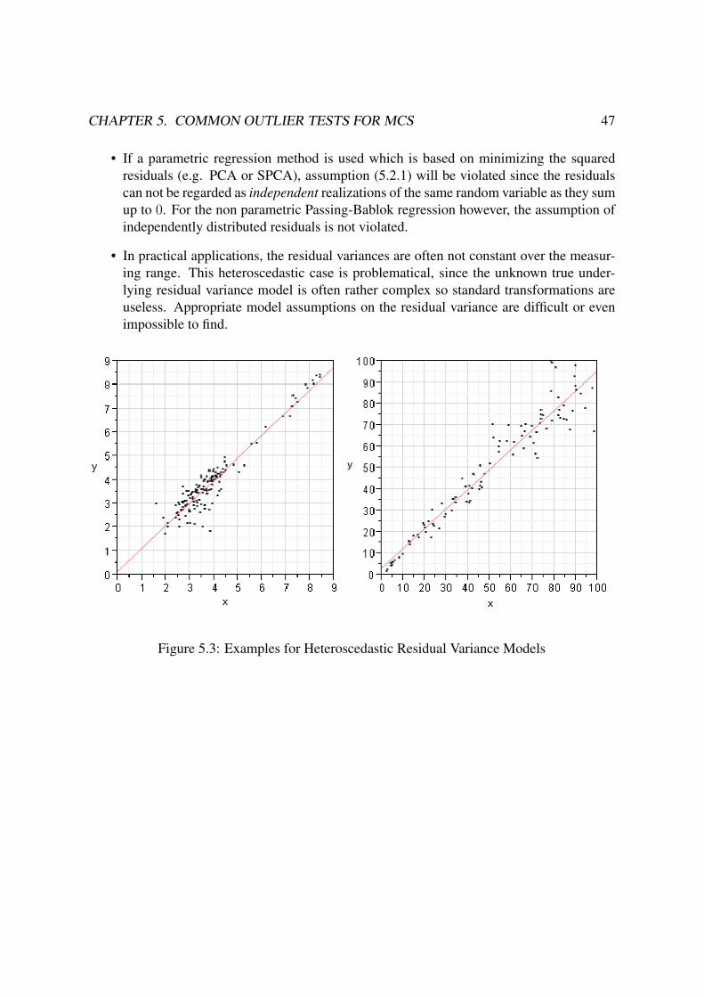
CHAPTER 5. COMMON OUTLIER TESTS FOR MCS 47
• If a parametric regression method is used which is based on minimizing the squared
residuals (e.g. PCA or SPCA), assumption (5.2.1) will be violated since the residuals
can not be regarded as independent realizations of the same random variable as they sum
up to 0. For the non parametric Passing-Bablok regression however, the assumption of
independently distributed residuals is not violated.
• In practical applications, the residual variances are often not constant over the measur-
ing range. This heteroscedastic case is problematical, since the unknown true under-
lying residual variance model is often rather complex so standard transformations are
useless. Appropriate model assumptions on the residual variance are difficult or even
impossible to find.
Figure 5.3: Examples for Heteroscedastic Residual Variance Models
Chapter 6
The New LORELIA Residual Test
As it has been explored in Chapter 5, most outlier tests for method comparison studies de-
scribed in the literature are formulated exclusively for a fixed number of outlier candidates
and require very strong statistical assumptions on the measurement error variance model or
the residual variance model, respectively. If the true number of outliers is unknown and the
underlying error variances are rather complex, these tests are therefore very limited in use.
Also there exists a variety of different error models and respective data transformation rules
(compare for example the models proposed by [Hawkins, 2002], [Cheng, Ness, 1999] and
[Rocke, Lorenzato, 1995]), which allow to apply common outlier test like the test proposed
by [Wadsworth, 1990] to a wider range of data situations, this is not a satisfying solution to the
general problem. On the one hand, the choice of an appropriate data transformation rule is not
always obvious and requires a good knowledge of the different error models described in the
literature. Moreover this implies that every dataset should be handled differently as method
comparison studies correspond to very heterogeneous data situations. It would be much more
satisfying to suggest a general solution to the outlier problem independently of the underlying
error variance model. On the other hand, there exist data situation in which none of the data
transformations proposed in the literature are appropriate. So far, no outlier identification test
has been proposed for these non standard data situations.
In this chapter a new outlier identification test for method comparison studies, which is based
on Passing-Bablok regression will be presented. Passing-Bablok regression is chosen for the
following reasons:
(i.) It is very robust against the presence of outliers,
(ii.) It takes random errors in both variables into account,
(iii.) The measurement error variances are not required to be constant.
However, Passing-Bablok regression may be replaced by another robust regression method if
it fulfills the above requirements.
48
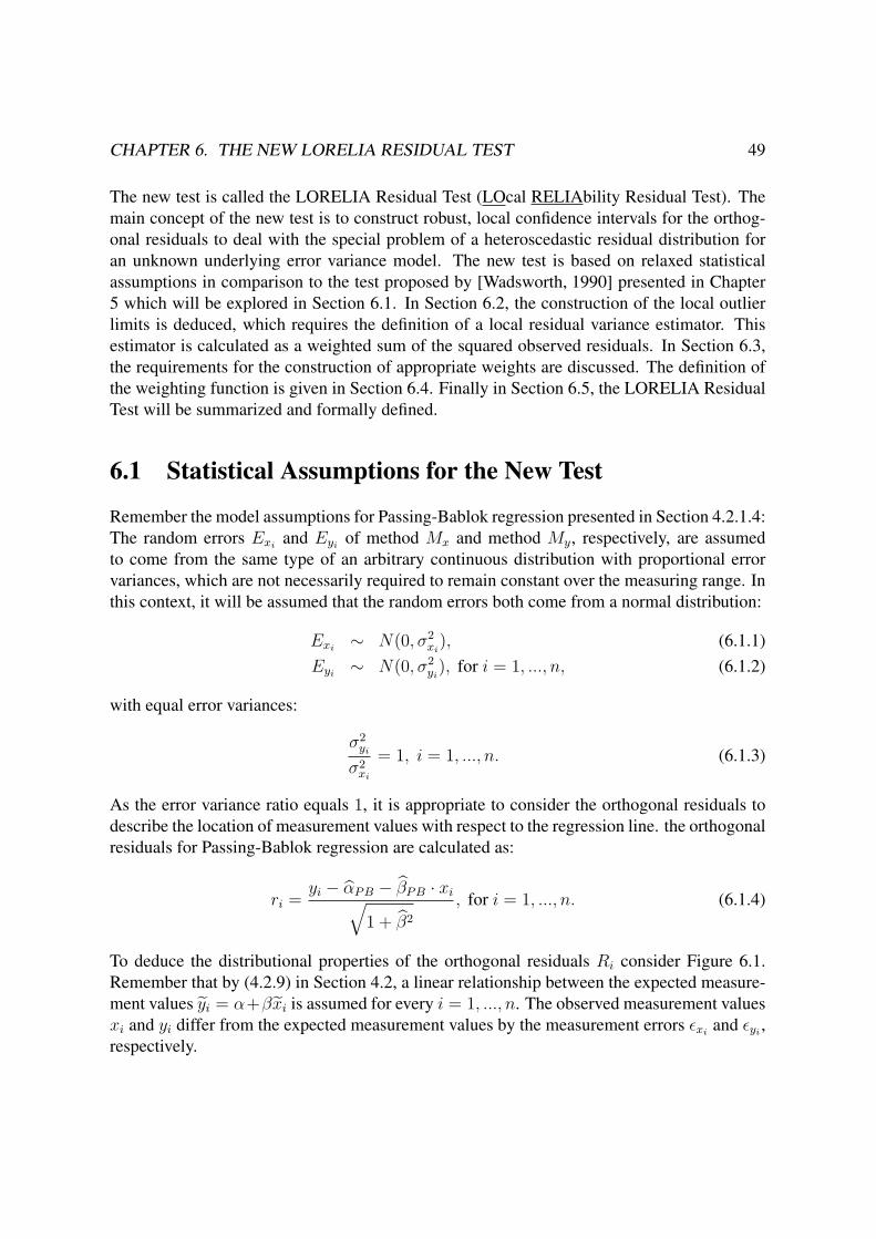
CHAPTER 6. THE NEW LORELIA RESIDUAL TEST 49
The new test is called the LORELIA Residual Test (LOcal RELIAbility Residual Test). The
main concept of the new test is to construct robust, local confidence intervals for the orthog-
onal residuals to deal with the special problem of a heteroscedastic residual distribution for
an unknown underlying error variance model. The new test is based on relaxed statistical
assumptions in comparison to the test proposed by [Wadsworth, 1990] presented in Chapter
5 which will be explored in Section 6.1. In Section 6.2, the construction of the local outlier
limits is deduced, which requires the definition of a local residual variance estimator. This
estimator is calculated as a weighted sum of the squared observed residuals. In Section 6.3,
the requirements for the construction of appropriate weights are discussed. The definition of
the weighting function is given in Section 6.4. Finally in Section 6.5, the LORELIA Residual
Test will be summarized and formally defined.
6.1 Statistical Assumptions for the New Test
Remember the model assumptions for Passing-Bablok regression presented in Section 4.2.1.4:
The random errors Exiand Eyi
of method Mx and method My, respectively, are assumed
to come from the same type of an arbitrary continuous distribution with proportional error
variances, which are not necessarily required to remain constant over the measuring range. In
this context, it will be assumed that the random errors both come from a normal distribution:
Exi∼ N(0, σ2
xi), (6.1.1)
Eyi∼ N(0, σ2
yi), for i = 1, ..., n, (6.1.2)
with equal error variances:
σ2yi
σ2xi
= 1, i = 1, ..., n. (6.1.3)
As the error variance ratio equals 1, it is appropriate to consider the orthogonal residuals to
describe the location of measurement values with respect to the regression line. the orthogonal
residuals for Passing-Bablok regression are calculated as:
ri =yi − αPB − βPB · xi√
1 + β2
, for i = 1, ..., n. (6.1.4)
To deduce the distributional properties of the orthogonal residuals Ri consider Figure 6.1.
Remember that by (4.2.9) in Section 4.2, a linear relationship between the expected measure-
ment values yi = α+βxi is assumed for every i = 1, ..., n. The observed measurement values
xi and yi differ from the expected measurement values by the measurement errors εxiand εyi
,
respectively.

CHAPTER 6. THE NEW LORELIA RESIDUAL TEST 50
Figure 6.1: The Orthogonal Residuals
By the Pythagorean Theorem the orthogonal residuals are realizations of:
Ri :=1√2(Exi
− Eyi) , for i = 1, ..., n.
Because of (6.1.1) and (6.1.2) it holds that:
(Exi− Eyi
) ∼ N(0, 2 · σ2xi), for i = 1, ..., n.
Hence, the residual distribution is given as:
Ri ∼ 1√2N(0, 2 · σ2
xi
)= N(0, σ2
xi) := N(0, σ2
ri), for i = 1, ..., n. (6.1.5)
The residual distribution thus correspond to the distribution of the random errors under the
assumption that the Passing-Bablok estimators αPB and βPB are unbiased estimates of the true
parameters α and β which determine the linear relationship between the unknown expected
measurement values. The residual variances σ2ri
are therefore approximately equivalent to
the measurement error variances and thus not necessarily constant over the measuring range.
Note again, that is is assumed here, that the residuals are statistically independent, which is
not an appropriate assumption for a parametric regression model (PCA or SPCA).
6.2 The Concept of Local Confidence Intervals
As pointed out in Section 5.2, outlier limits can be given in form of robust confidence inter-
vals for the orthogonal residuals. Since the orthogonal residual variance is not necessarily
constant, a local residual variance estimator is needed. The local residual variance will be
estimated from all observed residuals r1, ..., rn. Each residual will be weighted concerning

CHAPTER 6. THE NEW LORELIA RESIDUAL TEST 51
the information it contains for the specific local residual variance estimate under considera-
tion. The variance estimator will hence be constructed as the sum of weighted residuals with
appropriate weights wik. The LORELIA Residual Variance Estimator will be given as:
σ2ri=
1∑nl=1 wil
·n∑
k=1
wik · r2k, for i = 1, ..., n. (6.2.1)
Note that (6.2.1) is based on the assumption that:
E(Ri) = 0, for all i = 1, .., n.
[Satterthwaite, 1941] pointed out that a complex variance estimator like (6.2.1), will have
approximately the following distributional property:
DFi · σ2Ei
σ2Ei
approx∼ χ2DFi
, for i = 1, ..., n,
where DFi are the corresponding degrees of freedom calculated from the formula:
DFi =
(1∑n
k=1 wik·∑n
k=1 wik · r2k
)2
1
(∑n
k=1 wik)2 ·∑n
k=1 w2ik · r4
k
=(∑n
k=1 wik · r2k)
2∑nk=1 w2
ik · r4k
, for i = 1, ..., n, (6.2.2)
which is given in ([Satterthwaite, 1941], page 313) and ([Satterthwaite, 1946], page 111).
Note that in [Qian, 1998] it is shown that this formula may underestimate the effective de-
grees of freedom. Some approaches to correct this downward bias are discussed, which are
however not applied in the context of this work for the sake of simplicity.
By (6.1.5), it holds that:
Ri
σri
iid∼ N(0, 1), for i = 1, ..., n.
Thus, by (6.2.2) and (6.2.3) it follows with [Fahrmeir et al., 2007] (Chapter B, Page 461) that:√DFi · Ri
σri
· σri√DFi · σri
=Ri
σri
approx∼ tDFi, for i = 1, ..., n. (6.2.3)
With (6.2.3) it is easy to deduce a (1 − α)% approximative confidence interval for the ith
orthogonal residual:
Cα,i := [−tDFi,(1−α2) · σri
, tDFi,(1−α2) · σri
], for i = 1, ..., n. (6.2.4)
The confidence intervals (6.2.4) will be used as the local outlier limits in the following. The
definition of these outlier limits implies that outliers correspond to residuals which are very
unlikely to come from the corresponding normal distribution N(0, σ2ri).

CHAPTER 6. THE NEW LORELIA RESIDUAL TEST 52
Each residual ri which lays outside its corresponding confidence interval Cα,i will be identi-
fied as an outlier. This correspond to a multiple test situation as described in Section 3.1.2.
In order to keep a global significance level of αglob, the local significance levels has to be
adjusted. Thus every residual ri is compared to Cαloci,i where the αloci’s are determined by the
chosen adjustment procedure.
6.3 How to Weight - Newly Developed Criteria
The new outlier test is based on the construction of local confidence limits, which depend on
a weighted residual variance estimator. Hence, the main task of this work will be to construct
powerful weights. The new weighting method of the LORELIA Residual Test go back to a
weighting procedure proposed in [Konnert, 2005] which will be presented in Section 6.3.1. In
Section 6.3.2, new concept for the construction of improved weights will be presented.
6.3.1 Historical Background - Basic Ideas
The weights proposed in [Konnert, 2005] are given by:
wKonik :=
1
1 + δik
, for i, k = 1, ..., n, (6.3.1)
where
δik := (xpi − xp
k)2 + (yp
i − ypk)
2, for i, k = 1, ..., n
and (xpi , y
pi ) is the orthogonal projection of (xi, yi) to the regression line, given by:
xpi =
xi + βPB(yi − αPB)
1 + β2PB
, ypi = βPB · xp
i + αPB, for i = 1, ..., n.
Figure 6.2: Distance between the Orthogonal Residuals

CHAPTER 6. THE NEW LORELIA RESIDUAL TEST 53
By (6.3.2), the δik’s are given as the squared distances between the orthogonal projections to
the regression line. The weights wKonik generally decrease with increasing distances δik. It is
easy to see that wKonik ∈ (0, 1] for all i, k = 1, ..., n and that:
wKonik → 1 as δik → 0,
wKonik → 0 as δik →∞, for all i, k = 1, ..., n.
The definition of the weights in (6.3.1) is strongly related to the ’Inverse Distance Method’,
also called the ’Shepard’s Method’ proposed by [Shepard, 1968], which is used for interpola-
tion. The Shepard’s weights are given as:
wShepik :=
1
δik
, for i, k = 1, ..., n.
Note that, for the interpolation problem it always holds that δik �= 0 for i, k = 1, ..., n, unlike
for the weighting problem in the context of this work.
The residual variance estimator based on the weights defined in (6.3.1) can be biased by the
presence of outliers. In order to protect against masking effects, [Konnert, 2005] proposed to
neglect the largest term of wKonik · r2
k in formula (6.2.1). With:
wmi:= max
{wi1 · r2
1, wi2 · r22, ..., win · r2
n
}. (6.3.2)
the residual variance estimator thus becomes:
σ2ri=
1n∑
k=1k �=mi,
wKonik
·n∑
k=1k �=mi
wKonik · r2
k, for i = 1, ..., n. (6.3.3)
6.3.1.1 Problems and Limitations
The weights proposed in (6.3.1) are based on the distance measure δik. This insures that
that the residual variance is locally estimated as the weights decrease with increasing distance
between the corresponding orthogonal projections. However there exists severe disadvantages
and problems coming along with this definition of the weights, which will be explored in the
following:
(i.) A major disadvantage of the above weighting method is the fact that it is not robust
against outliers. Although the term wimi· r2
midefined in (6.3.2) is excluded in the
calculation of (6.2.1) to avoid masking effects, this does not necessarily contribute to
more stable residual variance estimates: On the one hand, (xmi, ymi
) does not necessar-
ily have to be an outlier, on the other hand, there may be more then one outlier in the
neighborhood of the ith residual. To visualize the above problems, consider the Passing-
Bablok regression fit and the corresponding residual plot for the following simulated
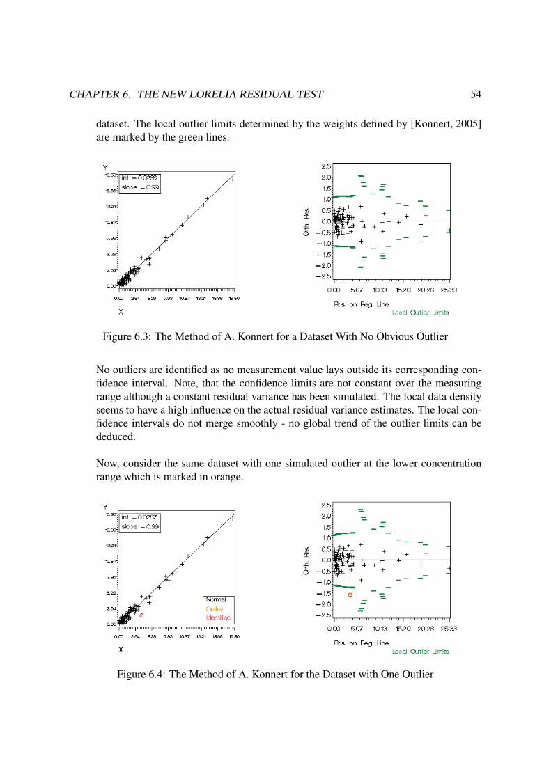
CHAPTER 6. THE NEW LORELIA RESIDUAL TEST 54
dataset. The local outlier limits determined by the weights defined by [Konnert, 2005]
are marked by the green lines.
Figure 6.3: The Method of A. Konnert for a Dataset With No Obvious Outlier
No outliers are identified as no measurement value lays outside its corresponding con-
fidence interval. Note, that the confidence limits are not constant over the measuring
range although a constant residual variance has been simulated. The local data density
seems to have a high influence on the actual residual variance estimates. The local con-
fidence intervals do not merge smoothly - no global trend of the outlier limits can be
deduced.
Now, consider the same dataset with one simulated outlier at the lower concentration
range which is marked in orange.
Figure 6.4: The Method of A. Konnert for the Dataset with One Outlier

CHAPTER 6. THE NEW LORELIA RESIDUAL TEST 55
The red circle indicates that the simulated outlier is well identified by the test. The
confidence limits look very similar to those for the data set without the outlier. Since
the outlier occurs in a high information density area, the negligence of wimi· r2
miavoids
that the presence of the outlier bias the surrounding residual variance estimates.
However, if a second outlier at the lower concentration range is added, the variance
estimates get strongly biased:
Figure 6.5: The Method of A. Konnert for the Dataset with Two Neighbored Outliers
Now, both outliers are not identified anymore. The confidence limits at the lower con-
centration range are much wider now than in the dataset with one or no outlier. At
the higher concentration range however, the width of the local confidence intervals has
hardly changed.
(ii.) Another deficiency is that the weights are not invariant under axes scaling, unlike the
similar Shepard’s method. A change of the unit of measurement in both methods will
lead to different values for the weights and thus to different variance estimates.
Theorem 6.1Let I1 be the measuring range of a given dataset. A scaled measuring range of I1 isdefined by I2 := F · I1 with F > 1. Let wKon
ik,I1and wKon
ik,I2denote the weights defined
in (6.3.1) with respect to I1 and I2, respectively. Then, the weights for the originalmeasuring range I1 and for the scaled measuring range I2 are related by:
wKonik,I1
= wKonik,I2
= 1, if i = k, (6.3.4)
wKonik,I1
< wKonik,I2
, if i �= k, for i = 1, ..., n. (6.3.5)
Proof: Equation (6.3.4) follows directly by the definition of the weights given in
[Konnert, 2005]. Now, choose i �= k for i, k ∈ {1, ..., n}. For a scaling factor F > 1 it
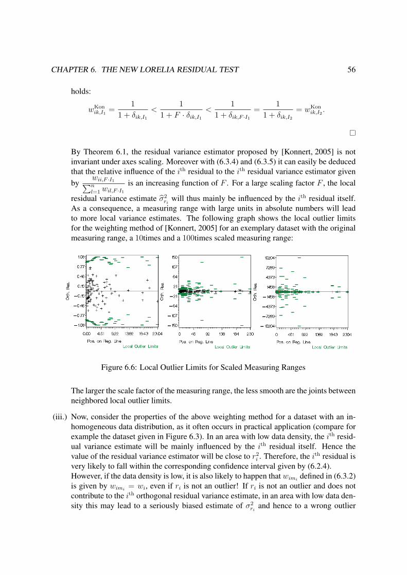
CHAPTER 6. THE NEW LORELIA RESIDUAL TEST 56
holds:
wKonik,I1
=1
1 + δik,I1
<1
1 + F · δik,I1
<1
1 + δik,F ·I1=
1
1 + δik,I2
= wKonik,I2
.
By Theorem 6.1, the residual variance estimator proposed by [Konnert, 2005] is not
invariant under axes scaling. Moreover with (6.3.4) and (6.3.5) it can easily be deduced
that the relative influence of the ith residual to the ith residual variance estimator given
bywii,F ·I1∑nl=1 wil,F ·I1
is an increasing function of F . For a large scaling factor F , the local
residual variance estimate σ2ri
will thus mainly be influenced by the ith residual itself.
As a consequence, a measuring range with large units in absolute numbers will lead
to more local variance estimates. The following graph shows the local outlier limits
for the weighting method of [Konnert, 2005] for an exemplary dataset with the original
measuring range, a 10times and a 100times scaled measuring range:
Figure 6.6: Local Outlier Limits for Scaled Measuring Ranges
The larger the scale factor of the measuring range, the less smooth are the joints between
neighbored local outlier limits.
(iii.) Now, consider the properties of the above weighting method for a dataset with an in-
homogeneous data distribution, as it often occurs in practical application (compare for
example the dataset given in Figure 6.3). In an area with low data density, the ith resid-
ual variance estimate will be mainly influenced by the ith residual itself. Hence the
value of the residual variance estimator will be close to r2i . Therefore, the ith residual is
very likely to fall within the corresponding confidence interval given by (6.2.4).
However, if the data density is low, it is also likely to happen that wimidefined in (6.3.2)
is given by wimi= wi, even if ri is not an outlier! If ri is not an outlier and does not
contribute to the ith orthogonal residual variance estimate, in an area with low data den-
sity this may lead to a seriously biased estimate of σ2ri
and hence to a wrong outlier

CHAPTER 6. THE NEW LORELIA RESIDUAL TEST 57
classification.
Generally, for areas with low data density, the local variance estimates will not be stable
since there is not much local data evidence. In dense data regions, closely neighbored
residuals have a high influence on the variance estimate which will lead to more sta-
ble estimates. In this case however, the variance estimates can easily get biased by the
presence of several outliers, as it has been shown in the above examples.
6.3.2 New Concepts for Weight Construction
In this section new concept for the construction of powerful weights will be presented. The
basic ideas by [Konnert, 2005] are improved and new ideas are developed.
6.3.2.1 Construction of a Local Estimator
In order to construct a local residual variance estimator, the residual variance estimate σ2ri
should be influenced more by the residuals which are closely neighbored to ri than by those
located far away. As a consequence, a measure for the distance between the residuals is
needed. Since the residuals are defined as the orthogonal distances to the regression line, a
distance measure for the orthogonal projections will be considered.
Figure 6.7: Influence of the Neighbored Residuals
The weights proposed in [Konnert, 2005] are exclusively based on a simple distance measure.
This insures that the residual variance estimator becomes local. However, there exist several
very important other requirements for an efficient weighting function, which will be presented
in the following.

CHAPTER 6. THE NEW LORELIA RESIDUAL TEST 58
6.3.2.2 Construction of an Outlier Robust Estimator
In order to achieve a residual variance estimator, which is robust against outliers, each residual
should be weighted according to its local reliability. The local reliability of a given residual
rk is high if the closely neighbored residuals are of the same magnitude. Residuals located far
away from rk may generally be of a very different magnitude and should therefore be consid-
ered less important when the reliability of rk is judged. The task is to construct a reliability
measure which is low for locally surprisingly large residuals. In this case, all neighbored
residuals are of much smaller magnitude. A reliability measure may therefore be based on the
sum of distance-weighted residual differences as it will be explored in Section 6.4.2.
Figure 6.8: The Local Reliability
In the above figure, the concepts of a high and a low local reliability are visualized.
6.3.2.3 Invariance under Axes Scaling
A change in the unit of measurement for both methods should have no influence on the val-
ues of the outlier limits. In order to achieve this, the weights should be invariant under axes
scaling. The most simple idea would be to standardize the measuring range in advance to
the calculation of the local outlier limits. Another idea is to construct relative measures for
the distance and for local reliability rather than absolute measures. In this work, the second
approach is chosen.
The constructed relative measures defined in Sections 6.4.1 and 6.4.2 involve the additional
information of the sample size which is neglected in the approach of [Konnert, 2005]. The

CHAPTER 6. THE NEW LORELIA RESIDUAL TEST 59
influence of the sample size is especially important to fulfill the requirements described in
Section 6.3.2.5.
6.3.2.4 The Meaning of the Local Data Information Density
The data density can differ a lot between different datasets and may even be very inhomoge-
neous within a single dataset. Thus, the (local) information density differs between and within
datasets. A lower information density should always correspond to wider outlier limits and
thus to a more conservative outlier test, as the level evidence for the outlier classification is
low. On the other hand, in densely distributed data regions, where the information density and
hence the level of evidence is high, existing outliers should be more easily identified.
Figure 6.9: Different Areas of Information Density
6.3.2.5 The Co-Domain of the Weights
The global co-domain Wn of the weights is determined by the highest and the lowest possible
weight for an arbitrary dataset with sample size n:
Wn :=
[inf
{i,k=1,...,n}{wik} , sup
{i,k=1,...,n}{wik}
], for an i = 1, ..., n.
The range of observed weights for a specific dataset
[min
{i,k=1,...,n}{wik} , max
{i,k=1,...,n}{wik}
]is
always a subset of Wn. The width of Wn should depend on the sample size n. For small
sample sizes, the amount of available information is limited. Therefore, none of the observed

CHAPTER 6. THE NEW LORELIA RESIDUAL TEST 60
residual should be radically down weighted. For high sample sizes, there is enough informa-
tion available to neglect a few of the observed residuals. Therefore, the width of the global
co-domain Wn should increase with increasing sample size n.
6.4 The Weights for the LORELIA Residual Test
In this section the weighting method for the new LORELIA Residual Test is presented. The
weights for the LORELIA Residual Test are given as the product of a distance measure Δik
and a measure for the local reliability Γk,n which depends on the sample size n as required in
Sections 6.3.2.1 and 6.3.2.2:
wik := Δik · Γk,n, for i, k = 1, ..., n. (6.4.1)
The distance measure Δik ensures, that the residual variance is locally estimated. The reliabil-
ity measure Γk,n is needed in order to construct a residual variance estimator which is robust
against outliers.
The distance and the reliability measure will be explicitly defined in Sections 6.4.1 and 6.4.2.
The properties of the new weights will be mathematically explored and it will be shown that
all the requirements given in Section 6.3.2 are fulfilled.
Note however, that there exist multiple possibilities to construct weights based on the prin-
ciple ideas presented in Section 6.3.2. Therefore, the weighting method for the LORELIA
Residual Test which has been developed in the context of this work should not be considered
as an exclusive solution to the general problem but may be further developed and improved.
6.4.1 Definition of the Distance Measure
In [Konnert, 2005] the squared distances δ2ik between the orthogonal projections are proposed
as a distance measure. The δik’s are transformed in the following way:
1
δik + 1, for i, k = 1, ..., n (6.4.2)
in order to achieve a co-domain of [0, 1] for the weights (compare Section 6.3.1). As it has
been already explored, this distance measure does not meet the requirement to be invariant
under axes scaling as claimed in Section 6.3.2.3. To achieve this, the absolute distances δik
are replaced by relative distances with respect to the mean distance. The mean distance is
given by:
δ =1
n2
n∑i=1
n∑k=1
δik. (6.4.3)

CHAPTER 6. THE NEW LORELIA RESIDUAL TEST 61
The considered relative distances are thus given as:
δik
δ, for i, k = 1, ..., n. (6.4.4)
The new LORELIA Distance Measure fulfills the requirements given in Section 6.3.2 as
shown in the following:
Definition 6.2 (The LORELIA Distance Weight)
The LORELIA Distance Weight is defined as:
Δik :=1
δik
δ+ 1
, for i, k = 1, ..., n. (6.4.5)
It is easy to see that:
Δii = 1, for i = 1, ..., n.
and
0 < Δik < 1, for i �= k, i, k = 1, ..., n.
The new distance measure (6.4.5) has the following important properties:
Theorem 6.3The LORELIA Distance Measure Δik defined in Definition 6.2 is invariant under axes scaling.
Proof: If I1 is the measuring range of a given dataset and I2 := F · I1, F > 1 is a scaled
measuring range, it holds:
Δik,I2 =1
n2δik,I2∑nl=1
∑nm=1 δlm,I2
+ 1
=1
n2·δik,F ·I1∑nl=1
∑nm=1 δlm,F ·I1
+ 1
=1
n2·F ·δik,I1∑nl=1
∑nm=1 F ·δlm,I1
+ 1
=1
n2δik,I1∑nl=1
∑nm=1 δlm,I1
+1+ 1
= Δik,I1 , for i, k = 1, .., n.

CHAPTER 6. THE NEW LORELIA RESIDUAL TEST 62
The new distance measure Δik takes account of different data densities as required in Section
6.3.2.4. In areas with low data density the distances between the residuals are large, thus all
distance weights Δik with k �= i are much smaller than Δii = 1. In high information density
areas however, all residuals rk which are closely neighbored to ri will have distance weights
Δik ≈ 1.
The following theorem insures that the requirements of Section 6.3.2.5 are met:
Theorem 6.4The co-domain for the LORELIA Distance Weights is given by:[
inf{i,k=1,...,n}
{Δik} , sup{i,k=1,...,n}
{Δik}]=
[1
n2
2·(n−1)+ 1
, 1
]. (6.4.6)
Proof: It is easy to see that:
sup{i,k=1,...,n}
{Δik} = 1.
In order to determine:
inf{i,k=1,...,n}
{Δik}calculate:
limδik→∞
Δik, for given i, k = 1, ..., n.
Without loss of generality, one may as well calculate:
limδ(i−1)i→∞
Δ(i−1)i, for a given i = 2, ..., n,
as illustrated in Figure 6.10:
Figure 6.10: Increasing Distance δ(i−1)i

CHAPTER 6. THE NEW LORELIA RESIDUAL TEST 63
It holds:
n2 · δ(i−1)i∑ns=1
∑nt=1 δst
=n2 · δ(i−1)i
2∑i−1
s=1
∑nt=i δst +
∑i−1s=1
∑i−1t=1 δst +
∑ns=i
∑nt=i δst
=n2 · δ(i−1)i
2(∑i−1
s=1
∑nt=i δ(i−1)i +
∑i−1s=1
∑nt=i
(δ(i−1)s + δit
))+∑i−1
s=1
∑i−1t=1 δst +
∑ns=i
∑nt=i δst
=n2
2∑i−1
s=1
∑nt=i 1 + 2
∑i−1s=1
∑nt=i
δ(i−1)s + δit
δ(i−1)i︸ ︷︷ ︸→ 0 for δ(i−1)i→∞
+
(∑i−1s=1
∑i−1t=1 δst +
∑ns=i
∑nt=i δst
)δ(i−1)i︸ ︷︷ ︸
→ 0 for δ(i−1)i→∞
→ n2
2(n− i+ 1)(i− 1), as δ(i−1)i →∞, for i = 2, ..., n.
Therefore:
Δ(i−1)i
δ(i−1)i→∞−→ 1n2
2·(n−i+1)(i−1)+ 1
≥ 1n2
2·min{i=2,...,n}{(n−i+1)·(i−1)} + 1
=1
n2
2(n−1)+ 1
. (6.4.7)
Thus, the co-domain for the Δik’s is given as:[inf
{i,k=1,...,n}{Δik} , sup
{i,k=1,...,n}{Δik}
]=
[1
n2
2·(n−1)+ 1
, 1
].
Therefore, it holds:[inf
{i,k=1,...,n}{Δik} , sup
{i,k=1,...,n}{Δik}
]→ [0, 1], for n →∞. (6.4.8)
With Theorem 6.3, it can easily be seen that the co-domain of the distance weights Δik and
thus also the co-domain of the overall weights wik = Δik · Γk,n is dependent of the sample
size n. Thus, the requirement given in Section 6.3.2.5 is fulfilled.

CHAPTER 6. THE NEW LORELIA RESIDUAL TEST 64
To illustrate the concept, consider for example the smallest possible distance weight for a
sample size of n = 10:
1102
2·(10−1)+ 1
≈ 0.1525,
which is about 10 times higher than the smallest possible weight for a sample size of n = 100:
11002
2·(100−1)+ 1
≈ 0.0194.
Hence, for a sample size of n = 100, the weights can scatter in a wider range than for a sample
size of n = 10. In Figure 6.11, the squared absolute distances δ21k to the 1st residual are plotted
against Δ1k for a dataset with n = 100 observations and a reduced dataset with n = 10observations. Since the second dataset is only a reduced version of the first, the absolute
distances between data values remain the same if the fact that the regression parameters will
change slightly is neglected.
Figure 6.11: The Values of the Distance Measure Δik for Different Sample Sizes
Although the absolute distances δ1k between the residuals remain the same for corresponding
measurement values, the actual range of values for the distance weights Δ1k is narrowed by
the reduction of the sample size.
6.4.2 Definition of a Reliability Measure
In this section a measure for the local reliability, as required in Section 6.3.2.2, will be con-
structed. The local reliability of a fixed residual rk is high, if closely neighbored residuals

CHAPTER 6. THE NEW LORELIA RESIDUAL TEST 65
are of the same magnitude. The local reliability of rk is low, if the surrounding residuals are
much smaller than rk (compare Figure 6.8). A reliability measure may therefore be based on
the weighted sum of differences between each residual and rk, where the weights are given
by the LORELIA Distance Measure Δik:
n∑l=1
Δlk · (|rl| − |rk|)2, k = 1, ..., n.
In order to construct a local reliability measure, which is invariant under axes scaling, as
claimed in Section 6.3.2.3, consider the relative sum of weighted differences between the
residuals:
γk,n :=
∑nl=1Δlk · (|rl| − |rk|)2∑n
m=1
∑ns=1Δms · (|rm| − |rs|)2 , for k = 1, ..., n. (6.4.9)
Note that the reliability measure γk,n depends on the sample size n. The values of γk,n gener-
ally decrease as n increases.
If rk is an outlier, γk,n will be close to 1. For a residual which is of the same magnitude
as the surrounding residuals, γk,n will be close to 0. The influence of the distance measure
Δlk in (6.4.9) guarantees, that the reliability is locally measured. Note that the local reliability
γk,n of a residual rk is the same for every residual variance estimate σ2i under consideration
and thus does not depend on i. The LORELIA Reliability Weight Γk,n will be given as a
function of γk,n:
Definition 6.5 (The LORELIA Reliability Weight)
For a constant parameter c > 1 the LORELIA Reliability Weight is defined as:
Γk,n :=
⎧⎪⎪⎪⎨⎪⎪⎪⎩1, for γk,n ≤ 1
n
0.5 ·[cos
((γk,n − 1
n) · π
cn+(c−1)
− 1n
)+ 1
]for 1
n< γk,n < c
n+(c−1)
0, for γk,n ≥ cn+(c−1)
.(6.4.10)
Thereby, c is a parameter to adjust the robustness of the outlier test for the given data
situation.
The LORELIA Reliability Weight Γk,n is based on the following considerations:
(i.) If the residual variances are assumed to be constant over the measuring range and no
outliers are present, then γk,n ≈ 1n
for all k = 1, ..., n. Hence, all residuals with γk,n ≤ 1n
will get a reliability weight of 1.

CHAPTER 6. THE NEW LORELIA RESIDUAL TEST 66
(ii.) If one residual out of n is c times larger or more than the remaining n− 1, this residual
will get the minimal reliability weight of 0. Thus, this residual does not influence the
variance estimates at all. The choice of the worst case limit cn+(c−1)
is important to
adjust the robustness of the variance estimator. If c is chosen too large, this will result
in false negative test results. Existing outliers may not be detected as only very extreme
residuals are classified as outliers. However, if c is chosen too small, the reliability
measure becomes too sensible for the normal data scattering which will result in many
false positive outlier identifications. Several values for the limit c has been tested by the
author in various data situations. Due to these experimental studies, it is recommended
to use a limiting value of:
c = 10. (6.4.11)
However, this value may not be appropriate for unusual or extreme data situations. It
will be the task of the data analyst to adjust the value of c in this case. In the context of
this work, the LORELIA Residual Test is always applied with c = 10.
(iii.) For residuals rk with 1n
< γk,n < cn+(c−1)
, the function
0.5 ·[cos
((γk,n − 1
n) · π
cn+(c−1)
− 1n
)+ 1
]is chosen to insure that Γk,n is a continuously differentiable, decreasing function in γk,n
over [0, 1], which is point symmetric in(0.5 ·
(1
n+
c
n+ (c− 1)
), f
(0.5 ·
(1
n+
c
n+ (c− 1)
))).
In the following graph, Γk,n is plotted as a function of γk,n for different sample sizes:
Figure 6.12: The Local Reliability Measure Γk,n for Different Sample Sizes and c = 10

CHAPTER 6. THE NEW LORELIA RESIDUAL TEST 67
6.5 Definition of the LORELIA Residual Test
In this section, the LORELIA Residual Test is summarized and formally defined to give a
general overview of the new test. The motivation for the given formulas and definitions are
given in the previous sections and will not be repeated here.
The new LORELIA Residual Test is explicitly formulated as follows:
Definition 6.6 (The LORELIA Test Hypotheses)
The LORELIA Residual Test is based on the following test hypotheses:
H0 : The considered dataset contains no outliers,
versus (6.5.1)
H1 : The considered dataset contains outliers.
H0 is rejected if any of the observed residuals ri exceeds the given outlier limits:
Reject H0 ⇔ ∃i ∈ {1, ..., n} : ri /∈ Cαloc,i, (6.5.2)
where Cαloc,iis an (1 − αloc)% approximate local confidence interval for the orthogonal
residual Ri.
As the multiple test situation (6.5.2) will lead to the accumulation of first order errors, the lo-
cal level of significance αloc has to be adjusted by an appropriate adjustment method in order
to keep a global significance level of αglob. A general discussion on this task has been given
in Section 3.1.2. Considerations on the choice of the adjustment methods for the LORELIA
Residual Test will be given in Section 7.4. An overview of different adjustment methods can
be found in [Hochberg, Tamhane, 1987] and [Hsu, 1996].
Outlier limits for the LORELIA Residual Test are given as local confidence intervals Cαloc,i
for the orthogonal residuals. These confidence intervals are defined as follows:

CHAPTER 6. THE NEW LORELIA RESIDUAL TEST 68
Definition 6.7 (The LORELIA Outlier Limits)
The LORELIA Outlier Limits are given by:
Cα,i := [−tDFi,(1−αloc2
) · σi, tDFi,(1−αloc2
) · σi], for i = 1, ..., n. (6.5.3)
where σ2i is a local residual variance estimator defined as:
σ2ri=
1∑nl=1 wil
·n∑
k=1
wik · r2k, for i = 1, ..., n. (6.5.4)
and tDFi,(1−αloc2
) is the (1−αloc)% quantile of the Student’s-t distribution with DFi degrees
of freedom calculated from the formula:
DFi =(∑n
k=1 wik · r2k)
2∑nk=1 w2
ik · r4k
, for i = 1, ..., n. (6.5.5)
The LORELIA Residual Variance Estimator is based on the following weighting function:
Definition 6.8 (The LORELIA Weights)
The LORELIA Weights are defined as:
wik := Δik · Γk,n, for i, k = 1, ..., n, (6.5.6)
where Δik is a measure for the distance between ri and rk along the regression line ,defined
in Definition 6.2 in Section 6.4.1, and Γk,n is a measure for the local reliability of rk which
depends on the sample size n and is defined in Definition 6.5 in Section 6.4.2.
With the above definitions the LORELIA Residual Test is entirely defined.

Chapter 7
Performance of the New LORELIAResidual Test
In this chapter, the performance of the LORELIA Residual Test will be evaluated in order to
answer the following questions:
• In real data situations, does the LORELIA Residual Test identifies visually suspicious
values as outliers?
• For simulated data situations, are simulated outliers truly identified? How many outlier
misclassifications are there?
• In the case of Bonferroni adjusted outlier limits, does the new test meet its predefined
significance level?
• What are the performance differences between the new LORELIA Residual Test and
the common outlier tests presented in Chapter 5?
• How good is the new test in standard data situations which can be handled with other
outlier tests?
• How good is the LORELIA Residual Test for more complex data situations in which
standard outlier tests will fail?
• Which factors influence the performance of the new test?
• Which problems and limitations can occur and how can they be handled?
• How does the choice of the adjustment procedure influence the performance of the
LORELIA Residual Test?
The new LORELIA Residual Test will be used on a variety of different datasets in order to
answer the above questions. Thereby, the performance of the test strongly depends on the
underlying data situation. Different datasets are classified concerning the following criteria:
69

CHAPTER 7. PERFORMANCE OF THE NEW LORELIA RESIDUAL TEST 70
(i.) The distribution of the measurement values within the measuring range,
(ii.) The underlying residual variance model,
(iii.) The number of outliers in the dataset,
(iv.) The magnitude of the outlier terms,
(v.) The position and the distribution of outliers.
Throughout this chapter, the LORELIA Residual Test is used for a global significance level
of αglob = 0.1 which is adjusted with the conservative Bonferroni procedure to insure that
the type 1 error is at most αglob as measurement values which are wrongly identified as out-
lier cause much additional work and troubles. The local significance level is thus given by
αloc =αglob
n.
To begin with, in Section 7.1, the LORELIA Residual Test will be compared to the com-
mon outlier tests for method comparison studies proposed by [Wadsworth, 1990], which are
presented in Chapter 5.
In Section 7.1.1, all tests will be applied on a variety of exemplary datasets in order to give a
first impression on the performance of the different tests. These datasets represent common
data situations which can be met in clinical practice. It will be checked visually which test
identifies suspicious values best and if the calculated outlier limits seem appropriate.
As the test performance strongly depends on the underlying data situations, a general rank-
ing of the different outlier tests is not possible. However, the LORELIA Residual Test often
outperforms the common global outlier tests presented in Chapter 5. In Section 7.1.2, the
superiority of the LORELIA Residual test is theoretically proven for a simple data model.
In Section 7.1.3, all outlier tests are compared on a variety of different simulated datasets
which represent the most common data situations in practical applications. As the outlier tests
of [Wadsworth, 1990] presented in Chapter 5 are all global outlier tests, the fact if the data
distribution within the measuring range is homogeneous or not will not influence the perfor-
mance of these tests. The position of existing outliers within the measuring range does not
influence the performance of global outlier tests, as well. The test performance of the LORE-
LIA Residual test however will be influenced by both criteria. Therefore the comparison is
done for homogeneously distributed datasets which differ only with respect to the criteria (ii.)
to (iv.). A performance ranking is given by comparing the correctness of the test results: A
good outlier test should identify as many true outliers as possible (true positive test results)
without wrongly declaring measurement values which belong to the population of interest as
outliers (false positive test results). The true affiliation of measurement values to the popula-
tion of interest Pint or to the contaminating population Pcont is usually not known for real data
situations. Therefore the tests are compared on simulated datasets which contain predefined
outliers.
Unlike the other outlier tests for method comparison studies presented in this work, the LORE-
LIA Residual Test is a local outlier test. Thus, its performance will be influenced by the

CHAPTER 7. PERFORMANCE OF THE NEW LORELIA RESIDUAL TEST 71
distribution of measurement values within the measuring range and by the position of exist-
ing outliers. In Section 7.2, the influence of the outlier position on the performance of the
LORELIA Residual Test will be evaluated for homogeneous and inhomogeneous distributed
datasets by a simulation study, compare criteria (i.) and (v.).
The LORELIA Residual Test is only appropriate if the local residual variances do not change
to drastically over the measuring range and if the sample distribution is not too inhomoge-
neous. This problem is discussed in Section 7.3 and a solution is suggested.
The performance of the new test is influenced by the choice of the adjustment procedure
for the local significance levels. Throughout this chapter, the LORELIA Residual Test was
applied with respect to the Bonferroni adjusted local outlier limits. In Section 4.1.13, the
choice of this adjustment procedure is discussed an an alternative method is proposed.
In Section 7.5 the results of this chapter are summarized.
All simulations in this chapter were programmed in SAS® 9.1. The underlying random num-
ber generator is based on the SAS® function RANUNI which is described in
[SAS Insitute Inc., 2008]. Uniformly distributed random numbers on the interval [0, 1] are
generated with the pseudo random number generator proposed by [Fishman, Moore, 1982]
which is given as follows:
xn+1 = (397204094 · xn)mod(231 − 1), for a seed value x0 ∈[0, 231 − 1
).
Other continuously distributed random numbers are generated with the help of the inverse
transform sampling method.
7.1 The LORELIA Residual Test in Comparison to Com-mon Outlier Tests
In this Section, the new LORELIA Residual Test will be compared to the outlier tests pre-
sented in Chapter 5. Thereby, remember that by (6.1.5) in Section in 6.1, the distribution
of the orthogonal residuals for Passing-Bablok regression is approximately equivalent to the
distribution of the measurement errors in method Mx and My. Therefore, it holds:
• If the residual variance is constant σ2ri≡ σ2, assumptions (4.1.3) and (4.1.4) of Section
4.1.1 are fulfilled and thus the absolute differences Dabsi are normally distributed which
corresponds to assumption (4.1.6). Therefore the global test of [Wadsworth, 1990]
based on the absolute differences and the one for the orthogonal residuals are expected
to deliver similar results.
• If a constant coefficient of variance is given σ2ri= c2
i · σ2, assumptions (4.1.12) and
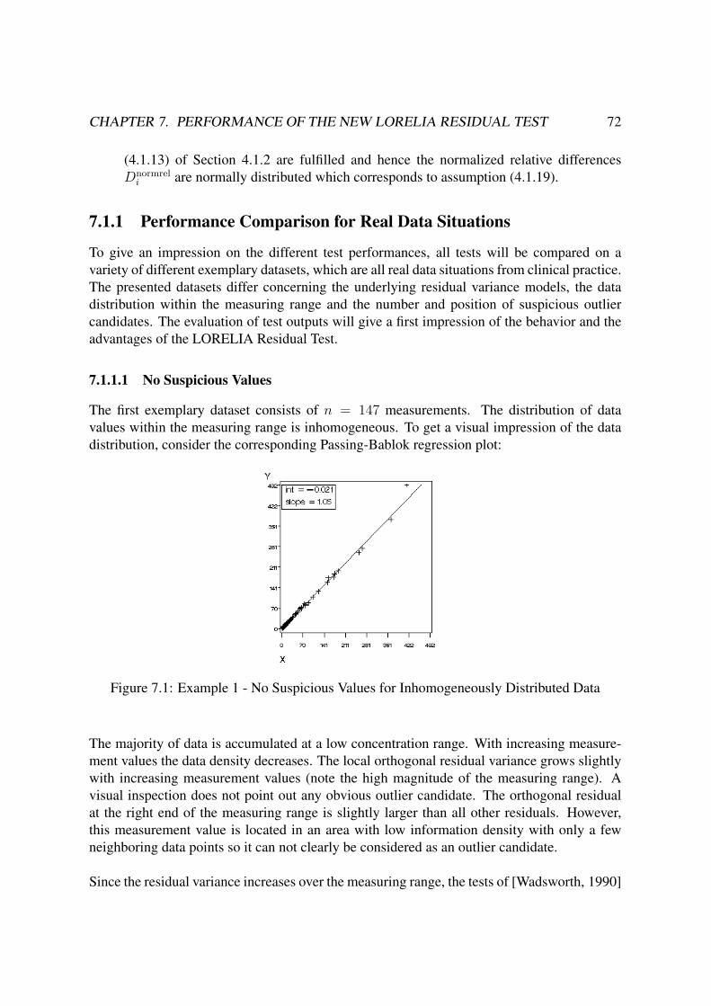
CHAPTER 7. PERFORMANCE OF THE NEW LORELIA RESIDUAL TEST 72
(4.1.13) of Section 4.1.2 are fulfilled and hence the normalized relative differences
Dnormreli are normally distributed which corresponds to assumption (4.1.19).
7.1.1 Performance Comparison for Real Data Situations
To give an impression on the different test performances, all tests will be compared on a
variety of different exemplary datasets, which are all real data situations from clinical practice.
The presented datasets differ concerning the underlying residual variance models, the data
distribution within the measuring range and the number and position of suspicious outlier
candidates. The evaluation of test outputs will give a first impression of the behavior and the
advantages of the LORELIA Residual Test.
7.1.1.1 No Suspicious Values
The first exemplary dataset consists of n = 147 measurements. The distribution of data
values within the measuring range is inhomogeneous. To get a visual impression of the data
distribution, consider the corresponding Passing-Bablok regression plot:
Figure 7.1: Example 1 - No Suspicious Values for Inhomogeneously Distributed Data
The majority of data is accumulated at a low concentration range. With increasing measure-
ment values the data density decreases. The local orthogonal residual variance grows slightly
with increasing measurement values (note the high magnitude of the measuring range). A
visual inspection does not point out any obvious outlier candidate. The orthogonal residual
at the right end of the measuring range is slightly larger than all other residuals. However,
this measurement value is located in an area with low information density with only a few
neighboring data points so it can not clearly be considered as an outlier candidate.
Since the residual variance increases over the measuring range, the tests of [Wadsworth, 1990]
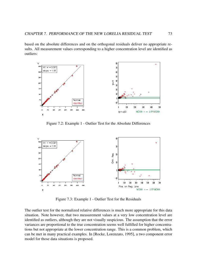
CHAPTER 7. PERFORMANCE OF THE NEW LORELIA RESIDUAL TEST 73
based on the absolute differences and on the orthogonal residuals deliver no appropriate re-
sults. All measurement values corresponding to a higher concentration level are identified as
outliers:
Figure 7.2: Example 1 - Outlier Test for the Absolute Differences
Figure 7.3: Example 1 - Outlier Test for the Residuals
The outlier test for the normalized relative differences is much more appropriate for this data
situation. Note however, that two measurement values at a very low concentration level are
identified as outliers, although they are not visually suspicious. The assumption that the error
variances are proportional to the true concentration seems well fulfilled for higher concentra-
tions but not appropriate at the lower concentration range. This is a common problem, which
can be met in many practical examples. In [Rocke, Lorenzato, 1995], a two component error
model for those data situations is proposed.

CHAPTER 7. PERFORMANCE OF THE NEW LORELIA RESIDUAL TEST 74
Figure 7.4: Example 1 - Outlier Test for the Normalized Relative Differences
Now, the test results obtained from the new LORELIA Residual Test are considered. The
Bonferroni adjusted local significance levels αloc for this exemplary dataset are given by:
αloc =αglob
n=
0.1
147≈ 0.00068.
The output plots are given as follows:
Figure 7.5: Example 1 - The LORELIA Residual Test
Two outliers are identified, which lay just slightly outside their corresponding confidence in-
tervals. One of it correspond to the largest measurement value discussed above. Another
measurement value in the middle of the measuring range lays just slightly inside its corre-
sponding confidence interval and is thus not identified as an outlier.
The local confidence limits merge smoothly and get wider with increasing concentration. This
is due to the increasing residual variance on the one hand and to the decreasing data density

CHAPTER 7. PERFORMANCE OF THE NEW LORELIA RESIDUAL TEST 75
on the other hand as explored in Section 6.3.2.4.
It will be interesting to have a look at the reliability measures Γk,n for all residual rk with
k = 1, ..., n. The identified outliers should have small reliability measures to guarantee that
the residual variance estimates are not biased by the presence of the outliers. In the following,
the position of (xpk, y
pk) on the regression line is plotted against its corresponding reliability
measure Γk,n for k = 1, ..., n:
Figure 7.6: Example 1 - Reliability Plot with Identified Outliers
Both outliers have a reliability weight of 0. The value which lay just slightly inside its outlier
limits is severely down weighted, as well. This value might have been detected as an outlier,
if a less conservative adjustment method would have been chosen. This points out that the
formal identification of outliers should always be accompanied by a visual data inspection by
a data analyst experienced in the field.
Values at the low concentration range all have reliability weights near 1. For higher con-
centrations, several values are down weighted by a small amount. This however does not lead
to the identification of many outliers. A single residual is only truly down weighted in the con-
sidered residual variance estimator, if all surrounding residual weights are higher. Therefore
a low reliability weight does not necessarily correspond to a low overall weight.
7.1.1.2 One Outlier Candidate
The second exemplary dataset has a sample size of n = 46. The data distribution is again
inhomogeneous. One obvious outlier candidate can be visually identified:

CHAPTER 7. PERFORMANCE OF THE NEW LORELIA RESIDUAL TEST 76
Figure 7.7: Example 2 - One Outlier Candidate for Inhomogeneously Distributed Data
The outlier test of [Wadsworth, 1990] for the absolute differences delivers the following re-
sults:
Figure 7.8: Example 2 - Outlier Test for the Absolute Differences
Again the majority of measurement values at the high concentration range is identified as
outliers. The scatter plot reveals that the absolute differences are not normally distributed
here. The test based on the orthogonal residual delivers similar results:

CHAPTER 7. PERFORMANCE OF THE NEW LORELIA RESIDUAL TEST 77
Figure 7.9: Example 2 - Outlier Test for the Residuals
The test for the normalized relative differences performs better, although the outlier limits
seem to narrow as a total number of five outliers is identified. This may be due to the fact, that
no adjustment of the global significance level for this multiple test situation is done.
Figure 7.10: Example 2 - Outlier Test for the Normalized Relative Differences
Now, calculate the Bonferroni adjusted confidence limits for the LORELIA Residual Test:
αloc =αglob
n=0.1
46≈ 0.0022.
The test results are given as follows:
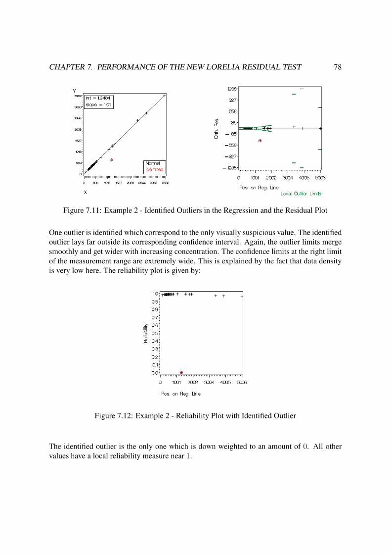
CHAPTER 7. PERFORMANCE OF THE NEW LORELIA RESIDUAL TEST 78
Figure 7.11: Example 2 - Identified Outliers in the Regression and the Residual Plot
One outlier is identified which correspond to the only visually suspicious value. The identified
outlier lays far outside its corresponding confidence interval. Again, the outlier limits merge
smoothly and get wider with increasing concentration. The confidence limits at the right limit
of the measurement range are extremely wide. This is explained by the fact that data density
is very low here. The reliability plot is given by:
Figure 7.12: Example 2 - Reliability Plot with Identified Outlier
The identified outlier is the only one which is down weighted to an amount of 0. All other
values have a local reliability measure near 1.
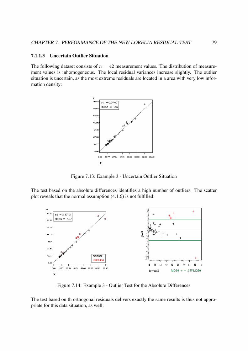
CHAPTER 7. PERFORMANCE OF THE NEW LORELIA RESIDUAL TEST 79
7.1.1.3 Uncertain Outlier Situation
The following dataset consists of n = 42 measurement values. The distribution of measure-
ment values is inhomogeneous. The local residual variances increase slightly. The outlier
situation is uncertain, as the most extreme residuals are located in a area with very low infor-
mation density:
Figure 7.13: Example 3 - Uncertain Outlier Situation
The test based on the absolute differences identifies a high number of outliers. The scatter
plot reveals that the normal assumption (4.1.6) is not fulfilled:
Figure 7.14: Example 3 - Outlier Test for the Absolute Differences
The test based on th orthogonal residuals delivers exactly the same results is thus not appro-
priate for this data situation, as well:

CHAPTER 7. PERFORMANCE OF THE NEW LORELIA RESIDUAL TEST 80
Figure 7.15: Example 3 - Outlier Test for the Residuals
The test for the normalized relative differences however is more appropriate here. One outlier
is identified which is slightly larger than the surrounding residuals.
Figure 7.16: Example 3 - Outlier Test for the Normalized Relative Differences
For the LORELIA Residual Test with a local level of significance given by
αloc =αloc
n=0.1
42≈ 0.0024
no outlier at all is identified:

CHAPTER 7. PERFORMANCE OF THE NEW LORELIA RESIDUAL TEST 81
Figure 7.17: Example 3 - The LORELIA Residual Test
However, the measurement value which was identified as an outlier by the test of
[Wadsworth, 1990] based on the normalized differences lays just slightly inside its corre-
sponding confidence limits and corresponds to the value with the lowest reliability measure
within the dataset:
Figure 7.18: Example 3 - Reliability Plot
Remember, that the Bonferroni correction can lead to a notable loss of power. For a less
conservative adjustment procedure, the LORELIA Residual Test will therefore deliver the
same results as the test based on normalized relative differences.

CHAPTER 7. PERFORMANCE OF THE NEW LORELIA RESIDUAL TEST 82
7.1.1.4 Decreasing Residual Variances
The following example represents the unusual case of a decreasing local residual variances.
Thus, none of the assumptions for the common outlier tests presented in Section 5 are fulfilled.
The sample size is given by n = 141.
Figure 7.19: Example 4 - Decreasing Residual Variance
The global outlier test based on the absolute differences identifies to many outliers at the low
concentration range:
Figure 7.20: Example 4 - Outlier Test for the Absolute Differences
The test for the orthogonal residuals is not appropriate either:

CHAPTER 7. PERFORMANCE OF THE NEW LORELIA RESIDUAL TEST 83
Figure 7.21: Example 4 - Outlier Test for the Residuals
The test based on the normalized relative differences performs even worse:
Figure 7.22: Example 4 - Outlier Test for the Normalized Relative Differences
The LORELIA Residual Test is done for a local significance level of
αloc =αloc
n=
0.1
141≈ 0.0007.
Only two outliers are identified which correspond to the most extreme observations. The local
outlier limits merge smoothly and model the trend of a decreasing residual variance well:
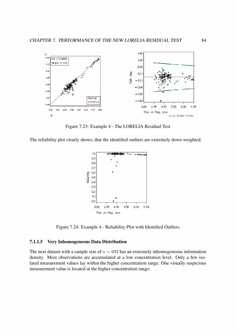
CHAPTER 7. PERFORMANCE OF THE NEW LORELIA RESIDUAL TEST 84
Figure 7.23: Example 4 - The LORELIA Residual Test
The reliability plot clearly shows, that the identified outliers are extremely down weighted:
Figure 7.24: Example 4 - Reliability Plot with Identified Outliers
7.1.1.5 Very Inhomogeneous Data Distribution
The next dataset with a sample size of n = 692 has an extremely inhomogeneous information
density. Most observations are accumulated at a low concentration level. Only a few iso-
lated measurement values lay within the higher concentration range. One visually suspicious
measurement value is located at the higher concentration range:

CHAPTER 7. PERFORMANCE OF THE NEW LORELIA RESIDUAL TEST 85
Figure 7.25: Example 5 - Very Inhomogeneous Data Dispersion
The Passing-Bablok slope estimator is mainly influenced by the cloud of low concentrated
values. Measurement values corresponding to a high concentration level are nearly all located
above the regression line. If a less robust regression method would be used like principal com-
ponent analysis, the fit would be better for the high concentrated samples due to a leverage
effect (compare Section 3.3.3). However in this case, most measurement values correspond-
ing to low concentration levels would be located above the regression line. Thus, the global
data trend is generally not well explained by a linear regression model.
Consider the outlier tests for the absolute differences:
Figure 7.26: Example 5 - Outlier Test for the Absolute Differences
Six Outliers are identified here. The identified outliers do not all correspond to extreme resid-
uals, which can be explained by the fact that the Passing-Bablok regression model is inappro-
priate for higher concentrations. The scatter plots can not really verify the normal assumption
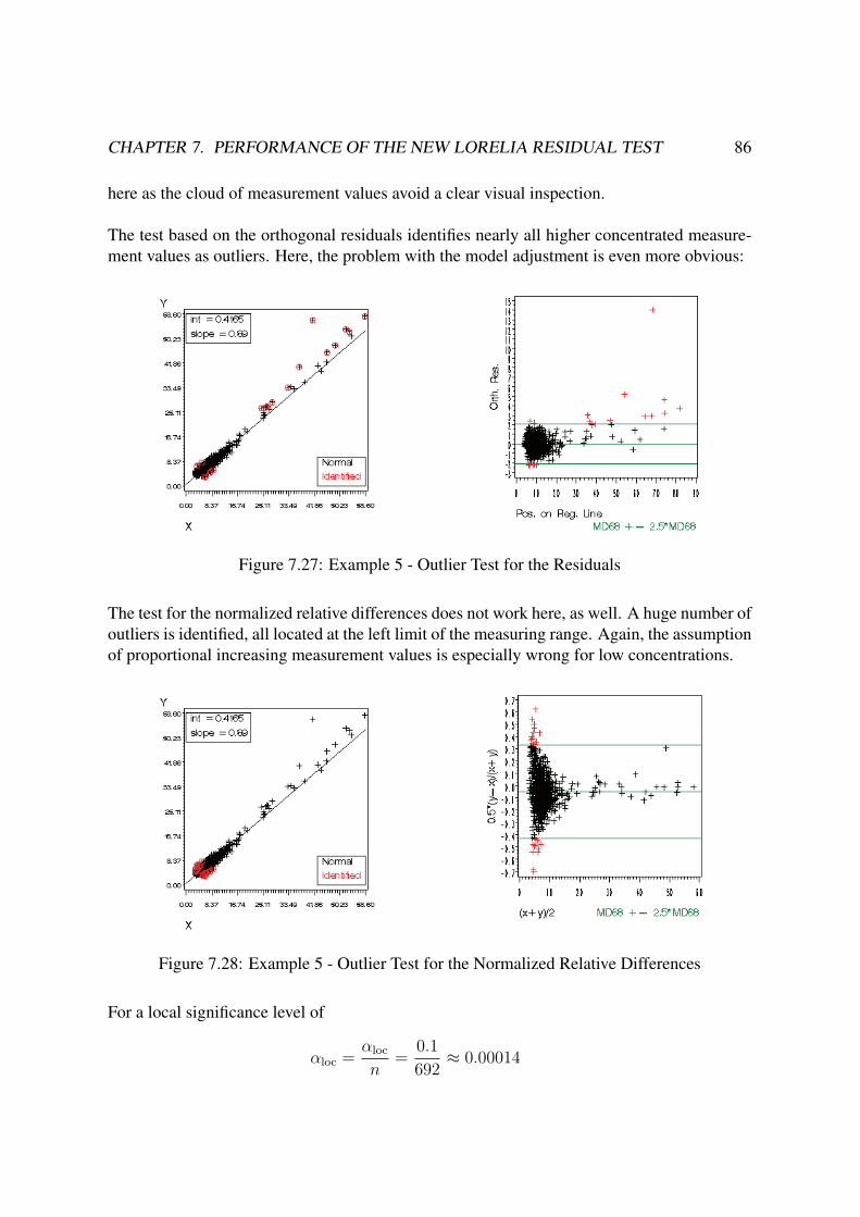
CHAPTER 7. PERFORMANCE OF THE NEW LORELIA RESIDUAL TEST 86
here as the cloud of measurement values avoid a clear visual inspection.
The test based on the orthogonal residuals identifies nearly all higher concentrated measure-
ment values as outliers. Here, the problem with the model adjustment is even more obvious:
Figure 7.27: Example 5 - Outlier Test for the Residuals
The test for the normalized relative differences does not work here, as well. A huge number of
outliers is identified, all located at the left limit of the measuring range. Again, the assumption
of proportional increasing measurement values is especially wrong for low concentrations.
Figure 7.28: Example 5 - Outlier Test for the Normalized Relative Differences
For a local significance level of
αloc =αloc
n=
0.1
692≈ 0.00014

CHAPTER 7. PERFORMANCE OF THE NEW LORELIA RESIDUAL TEST 87
the LORELIA Residual Test delivers the following result:
Figure 7.29: Example 5 - The LORELIA Residual Test
One outlier is identified which correspond to the visually suspicious value mentioned above.
Some other residuals lay just slightly inside their corresponding confidence intervals. The
reliability plot shows that several values are down weighted, but the identified outlier is the
only which is down weighted to an amount of 0:
Figure 7.30: Example 5 - Reliability Plot with Identified Outliers
Note that there exists a cloud of down weighted observations at the lower concentration range.
This however does not lead to the identification of a cloud of outliers, as they are all down
weighted to a similar amount! Remember that a single residual is only truly down weighted,
if all surrounding residual weights are higher.

CHAPTER 7. PERFORMANCE OF THE NEW LORELIA RESIDUAL TEST 88
7.1.1.6 Conclusion
The above real data examples represent a broad field of data situations in which the assump-
tion for common outlier tests are not (well) fulfilled. Therefore, the outliers tests proposed by
[Wadsworth, 1990] which are defined in Section 5 all deliver either wrong or misleading re-
sults. As the LORELIA Residual is based on relaxed statistical assumptions (compare Section
6.1), it clearly performs best for the presented examples. The following general observations
with respect to the performance of the LORELIA Residual Test can be made:
(i.) Visually suspicious values are well identified.
(ii.) The local confidence limits merge smoothly over the measuring range.
(iii.) The LORELIA Residual Test is more conservative in areas with low information density
than in areas with a high data density.
(iv.) There exist a trend of decreasing reliability when data density decreases. This does
not lead to outlier misclassification, since the reliability of a residual always has to be
compared to the reliabilities of the surrounding residuals.
7.1.2 Proof of Performance Superiority for an Exemplary Data Model
As pointed out above, the performance of an outlier test strongly depends on the underlying
data situations. Although, the LORELIA Residual Test often outperforms the common global
outlier tests proposed by [Wadsworth, 1990], the performance superiority of the new test is
difficult to prove for general data models, as the expected LORELIA Weights wik = Δik ·Γk,n
depend on many different influence factors such as the sample size, the underlying residual
variance model, the sample distribution within the measuring range and the number, the po-
sition and the magnitude of outliers. Moreover, the LORELIA Residual Test do not always
outperform all of the tests presented in Chapter 5, as the test for the absolute differences,
the test for the normalized relative differences and the test for the orthogonal residuals are
generally not expected to deliver the same results since they are based on different statistical
assumptions.
In this section, a simple model class M of method comparison datasets is defined for which
all tests presented in Chapter 5 are expected to deliver the same results. This model class is
defined such that the number of influence factors for the LORELIA Weights is reduced, which
allows to prove the general superiority of the LORELIA Residual Test for datasets belonging
to this model class. An exemplary dataset from this model class is evaluated with all outlier
tests in order to illustrate the theoretical result.
The model class M is defined as follows:

CHAPTER 7. PERFORMANCE OF THE NEW LORELIA RESIDUAL TEST 89
Definition 7.1 (The Model Class M of Method Comparison Datasets)
A dataset S of sample size n belongs to the model class M of method comparison datasets
if the following assumptions are fulfilled:
(i.) The observed measurement values of method Mx respective My are given as:
xi = xi + εxi, (7.1.1)
yi = yi + εyi, for i = 1, ..., n, (7.1.2)
where xi, yi are the expected measurement values and εxi, εxi
correspond to the ran-
dom errors.
(ii.) The expected measurement values are related by a linear relationship with slope 1and intercept 0:
xi = yi =: ci, for i = 1, ..., n, (7.1.3)
where ci denotes the true concentration of the ith sample. Without loss
of generality it will be assumed that the order of the measurement tuples
(x1, y1), (x2, y2), ..., (xn, yn) correspond to the order of increasing true concentra-
tions.
(iii.) The sample distribution within the measuring range is homogeneous.
(iv.) Let m be given such that m > n2. The random errors belonging to the first m obser-
vations are given as:
εxi= εyi
≡ 0, for i = 1, ...,m, (7.1.4)
which can be equally formulated as Exi, Eyi
∼ N(0, σ2i ), with σ2
i = 0 for i =1, ...,m. The remaining n−m random errors are realizations of:
Exi, Eyi
∼ N(0, σ2i ), for, i = m+ 1, ..., n, (7.1.5)
where σi is a multiple of the corresponding true sample concentration ci:
σi = c · ci, for all i = m+ 1, ..., n and a factor c > 0. (7.1.6)
Note that the measurement values belonging to a dataset in M are all determined by a pre-
defined random error model. Thus, the datasets contain no true outliers due to contamination
(compare Section 2.4.2).
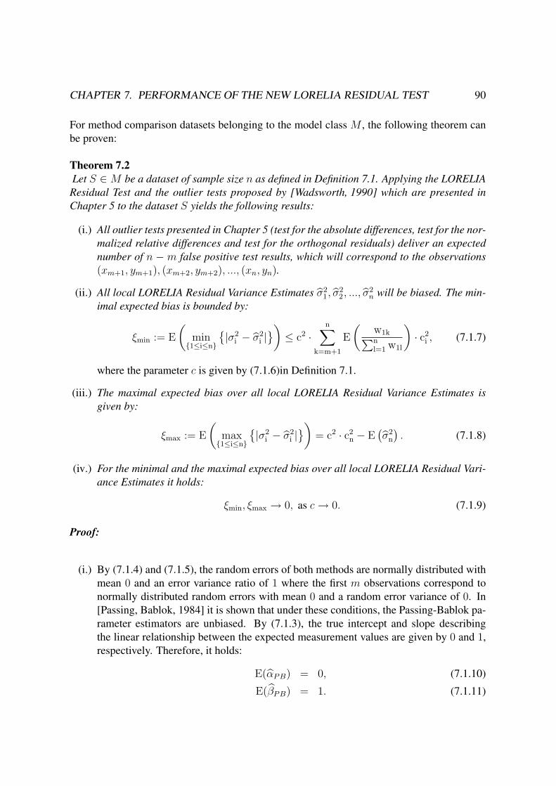
CHAPTER 7. PERFORMANCE OF THE NEW LORELIA RESIDUAL TEST 90
For method comparison datasets belonging to the model class M , the following theorem can
be proven:
Theorem 7.2Let S ∈M be a dataset of sample size n as defined in Definition 7.1. Applying the LORELIAResidual Test and the outlier tests proposed by [Wadsworth, 1990] which are presented inChapter 5 to the dataset S yields the following results:
(i.) All outlier tests presented in Chapter 5 (test for the absolute differences, test for the nor-malized relative differences and test for the orthogonal residuals) deliver an expectednumber of n −m false positive test results, which will correspond to the observations(xm+1, ym+1), (xm+2, ym+2), ..., (xn, yn).
(ii.) All local LORELIA Residual Variance Estimates σ21, σ
22, ..., σ
2n will be biased. The min-
imal expected bias is bounded by:
ξmin := E
(min
{1≤i≤n}
{|σ2i − σ2
i |}) ≤ c2 ·
n∑k=m+1
E
(w1k∑nl=1w1l
)· c2i , (7.1.7)
where the parameter c is given by (7.1.6)in Definition 7.1.
(iii.) The maximal expected bias over all local LORELIA Residual Variance Estimates isgiven by:
ξmax := E
(max{1≤i≤n}
{|σ2i − σ2
i |})
= c2 · c2n − E(σ2
n
). (7.1.8)
(iv.) For the minimal and the maximal expected bias over all local LORELIA Residual Vari-ance Estimates it holds:
ξmin, ξmax → 0, as c → 0. (7.1.9)
Proof:
(i.) By (7.1.4) and (7.1.5), the random errors of both methods are normally distributed with
mean 0 and an error variance ratio of 1 where the first m observations correspond to
normally distributed random errors with mean 0 and a random error variance of 0. In
[Passing, Bablok, 1984] it is shown that under these conditions, the Passing-Bablok pa-
rameter estimators are unbiased. By (7.1.3), the true intercept and slope describing
the linear relationship between the expected measurement values are given by 0 and 1,
respectively. Therefore, it holds:
E(αPB) = 0, (7.1.10)
E(βPB) = 1. (7.1.11)

CHAPTER 7. PERFORMANCE OF THE NEW LORELIA RESIDUAL TEST 91
From (7.1.4), (7.1.5), (7.1.10) and (7.1.11) it can be deduced that the random variables
for the absolute differences, for the normalized relative differences and for the orthogo-
nal residuals fulfill:
E(Dabsi )
E(Dnormreli )
E(Ri)
⎫⎬⎭ = 0, for i = 1, ..., n,
where Dabsi and Dnormrel
i are defined trough (4.1.5) and (4.1.18) in Chapter 4. As the
median is an unbiased estimator for the mean of normally distributed random variables,
it follows:
E(med(Dabs))E(med(Dnormrel))E(med(R))
⎫⎬⎭ = 0.
By (7.1.4) and (7.1.5), the expected order of the absolute deviations between the abso-
lute differences and their median is given by:
|Dabs1 −med(Dabs)| ≤ |Dabs
2 −med(Dabs)|≤ ...
≤ |Dabsm −med(Dabs)|
< |Dabsm+1 −med(Dabs)|
< ...
< |Dabsn −med(Dabs)|.
Thus by (ii.) in Definition 7.1, the expected order correspond to the order of increasing
concentrations ci. The same holds true for the expected order of the absolute devia-
tions between the normalized relative differences and their median or for the orthogonal
residuals.
By [Hartung et al., 2009] (Chaper XIV, Page 856), the 68% median absolute deviation
which is given as 1.4828 times the median absolute deviation, is an unbiased estimator
for the standard deviation of a normal distribution. By the above considerations, the
expected ranks of the absolute deviations between the respective comparison measures
and their median are expected to correspond to the order of the measurement values.
Thus, as m > n2, it holds by (7.1.4):
E(med(|Dabs −med(Dabs)|))
=
⎧⎨⎩E(|Dabs −med(Dabs)|(n+1
2)
), if n is odd,
E(0.5 ·
[|Dabs −med(Dabs)|(n
2) + |Dabs −med(Dabs)|(n+2
2)
]), if n is equal,
=
⎧⎨⎩E(|Dabs −med(Dabs)|n+1
2
), if n is odd,
E(0.5 ·
[|Dabs −med(Dabs)|n
2+ |Dabs −med(Dabs)|n+2
2
]), if n is equal,
= 0.

CHAPTER 7. PERFORMANCE OF THE NEW LORELIA RESIDUAL TEST 92
Equivalently, on may show that:
E(med(|Dnormrel −med(Dnormrel)|)) = 0,
E (med(|R−med(R)|)) = 0.
Hence, it holds:
E(mad68(Dabs)
)E(mad68(Dnormrel)
)E (mad68(R))
⎫⎬⎭ = 0.
Therefore, the expected global outlier limits defined by (5.1.1) and (5.2.2) in Section 5
are given by:
E(med(dabs)± 2.5 ·mad68(dabs)
)E(med(dnormrel)± 2.5 ·mad68(dnormrel)
)E (med(r)± 2.5 ·mad68(r))
⎫⎬⎭ = ±0.
Thus, all measurement values which correspond to a residual variance σ2i > 0, namely
observations (xm+1, ym+1), (xm+2, ym+2), ..., (xn, yn), are expected to be wrongly iden-
tified as outliers.
�(i.)
(ii.) The LORELIA Weights do not involve any model information of the underlying residual
variances in order to be globally applicable for every data situation. As the local residual
variances are not constant over the whole measuring range for datasets belonging to the
model class M , all local LORELIA Residual Variance Estimates will be biased due to
a smoothing effect. This bias will be minimal for the first measurement value (x1, y1)as the nearest m− 1 neighbors correspond to the same local residual variance of 0. It is
only slightly overestimated due to the remaining n−m measurement values which lay
far away from (x1, y1) and which correspond to residual variances greater than 0. Thus,
it holds:
ξmin := E
(min
{1≤i≤n}
{|σ2i − σ2
i |})
= E(σ2
1
).
An upper bound for expected value of the 1st LORELIA Residual Variance Estimate σ21
is calculated in the following. Thereby, remember that by Definition (6.5) of the LORE-
LIA Reliability Measure Γk,n in Section 6.4.2, the values of the LORELIA Weights wik
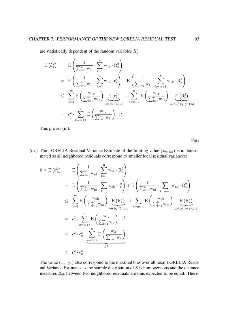
CHAPTER 7. PERFORMANCE OF THE NEW LORELIA RESIDUAL TEST 93
are statistically dependent of the random variables R2k.
E(σ2
1
)= E
(1∑n
l=1w1l
·n∑
k=1
w1k · R2k
)
= E
(1∑n
l=1w1l
·m∑
k=1
w1k · r2k)+ E
(1∑n
l=1w1l
·n∑
k=m+1
w1k · R2k
)
≤m∑
k=1
E
(w1k∑nl=1w1l
)E(r2k)︸ ︷︷ ︸
=0 by (7.1.4)
+n∑
k=m+1
E
(w1k∑nl=1w1l
)E(R2
k
)︸ ︷︷ ︸=c2·c2k by (7.1.5)
= c2 ·n∑
k=m+1
E
(w1k∑nl=1w1l
)· c2k.
This proves (ii.).
�(ii.)
(iii.) The LORELIA Residual Variance Estimate of the limiting value (xn, yn) is underesti-
mated as all neighbored residuals correspond to smaller local residual variances:
0 ≤ E(σ2
n
)= E
(1∑n
l=1wnl
·n∑
k=1
wnk · R2k
)
= E
(1∑n
l=1wnl
·m∑
k=1
wnk · r2k)+ E
(1∑n
l=1wnl
·n∑
k=m+1
wnk · R2k
)
≤m∑
k=1
E
(wnk∑nl=1wnl
)E(R2
k
)︸ ︷︷ ︸=0 by (7.1.4)
+n∑
k=m+1
E
(wnk∑nl=1wnl
)E(R2
k
)︸ ︷︷ ︸=c2·c2i by (7.1.5)
= c2 ·n∑
k=m+i
E
(wik∑nl=1wil
)· c2i
≤ c2 · c2n ·
n∑k=m+i
E
(wik∑nl=1wil
)︸ ︷︷ ︸
≤1
≤ c2 · c2n.
The value (xn, yn) also correspond to the maximal bias over all local LORELIA Resid-
ual Variance Estimates as the sample distribution of S is homogeneous and the distance
measures Δik between two neighbored residuals are thus expected to be equal. There-

CHAPTER 7. PERFORMANCE OF THE NEW LORELIA RESIDUAL TEST 94
fore, it holds:
ξmax := E
(max{1≤i≤n}
{|σ2i − σ2
i |})
= E(|σ2
n − σ2n|)
= c2 · c2n − E
(σ2
n
)> 0. (7.1.12)
This proves (iii.).
�(iii.)
(iv.) The proof of (iv.) follows directly from (ii.), (iii.) and (7.1.12).
�(iv.)
This completes the proof of Theorem 7.2.
Remark 7.3For datasets S ∈ M , the local LORELIA Residual Variances will generally be overestimated
at the low concentration range and underestimated for higher concentrations. Therefore, if
(xn, yn) is not falsely identified as an outlier, then there will be no false positive test results
at all. By Theorem 7.2 (iv.), the increment of the bias of σ2n is controlled by the magnitude of
the parameter c, defined in (7.1.6). However, the LORELIA Outlier Limits do not exclusively
depend on the residual variance estimate but also on the local adjusted significance level αloc.
A conservative adjustment of the global significance level such as the common Bonferroni
adjustment will balance the downward bias of σ2n to a certain extend.
For illustration, consider the following exemplary dataset belonging to the model class M :
Figure 7.31: Exemplary Dataset from the Model Class M
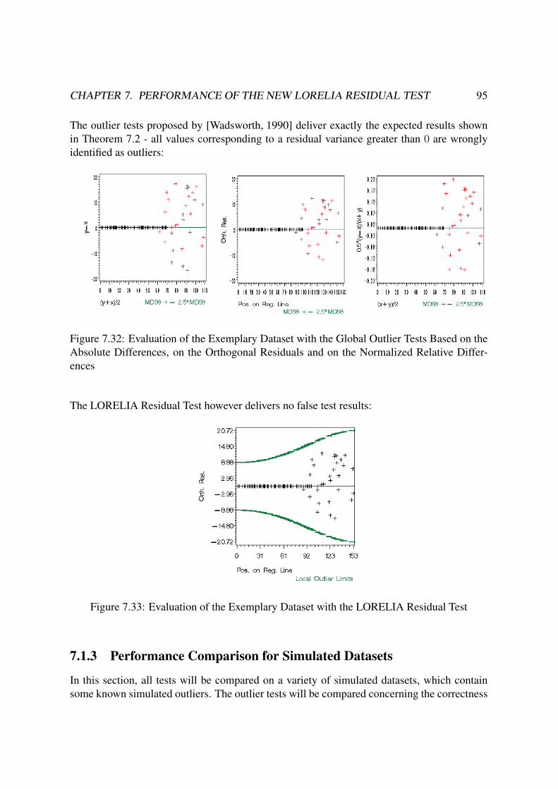
CHAPTER 7. PERFORMANCE OF THE NEW LORELIA RESIDUAL TEST 95
The outlier tests proposed by [Wadsworth, 1990] deliver exactly the expected results shown
in Theorem 7.2 - all values corresponding to a residual variance greater than 0 are wrongly
identified as outliers:
Figure 7.32: Evaluation of the Exemplary Dataset with the Global Outlier Tests Based on the
Absolute Differences, on the Orthogonal Residuals and on the Normalized Relative Differ-
ences
The LORELIA Residual Test however delivers no false test results:
Figure 7.33: Evaluation of the Exemplary Dataset with the LORELIA Residual Test
7.1.3 Performance Comparison for Simulated Datasets
In this section, all tests will be compared on a variety of simulated datasets, which contain
some known simulated outliers. The outlier tests will be compared concerning the correctness

CHAPTER 7. PERFORMANCE OF THE NEW LORELIA RESIDUAL TEST 96
of the test results, so to say the number of true positive and false positive test results. Thereby,
the comparison is done for different data situations to judge the influence of the underlying
residual variance model, the number of present outliers, the magnitude of the outlier terms
and the influence of the outlier distribution within the dataset.
7.1.3.1 Simulation Models
It is obvious that the test results do not uniquely depend on the choice of the outlier test but also
on the actual data situation. Therefore, several representative simulation models will be intro-
duced in this section which differ with respect to the criteria mentioned above. The general
notations for all data simulations have been introduced in Section 4. The special distribution
and parameter setting for the different simulation models are specified in the following. The
choice of these settings is to a certain extend arbitrary. It is motivated in intention to simulate
datasets which correspond well to common outlier scenarios in method comparison studies. In
the context of this work, the author examined a broad range of different experimental datasets,
which lead to the choice of the following simulation models.
Note that, unlike the LORELIA Residual Test, the outlier tests presented in Chapter 5 are
all global outlier tests which will not react to the local data density, which is a clear drawback
for an appropriate data analysis. The LORELIA Residual Test is more conservative in areas
with low data density than in dense data areas, whereas all other tests deliver their test results
independently of the local data density. Therefore, an outlier within an area of low local data
density may not be identified by the LOELIA Residual Test, which is hence a false negative
test result, whereas the outlier is well identified by a respective global test. However, the test
result of the LORELIA Residual Test is still more appropriate as it takes the local information
density into account. If the distribution of measurement values within the measuring range is
inhomogeneous, the test results of the LORELIA Residual Test can therefore not directly be
compared to the test results of the other tests. For this reason, the number of correct test results
is only an appropriate measure for a performance comparison in the case of a homogeneous
data distribution.
The different simulation models are given as follows. Consider a general sample size of:
n = 100. (7.1.13)
The expected measurement values of method Mx and My are assumed to be equal to the true
sample concentration:
xi = yi = ci, for i = 1, ..., n, (7.1.14)
which correspond to the case of equivalent methods Mx and My.
The true concentrations ci are homogeneously distributed within the measuring range:
Ci ∼ U(0, 100), i=1,...,n. (7.1.15)

CHAPTER 7. PERFORMANCE OF THE NEW LORELIA RESIDUAL TEST 97
The measurement values including the random errors are thus realizations of:
Xi ∼ ci +N(0, σ2ri) (7.1.16)
Yi ∼ ci +N(0, σ2ri), for i = 1, ..., n. (7.1.17)
Three different residual variance models are considered.
(i.) The most simplest case of a constant residual variance will be modeled by:
σ2ri≡ 0.1, for all i = 1, ..., n. (7.1.18)
(ii.) The case of a constant coefficient of variance as introduced in (4.1.14) in Section 4.1.2
is given by:
σ2ri= 0.01 · c2
i , for i = 1, ..., n. (7.1.19)
(iii.) The case of a non constant coefficient of variance is modeled as:
σ2ri= 4 + 0.01 · c2
i , for i = 1, ..., n. (7.1.20)
Outliers will be biased realizations of Xi and/or Yi. They will be modeled as:
Xi + outxi∼ Z + Exi
+ outxi(7.1.21)
Yi + outyi∼ xi + Eyi
+ outyi, for outxi
, outyi∈ R, i = 1, ..., n. (7.1.22)
If for an i = 1, ..., n, it holds that
outxi= outyi
�= 0, (7.1.23)
this correspond to a problem within the ith sample, like a false concentration or a somehow
contaminated sample. If
outxi�= outyi
and (outxi= 0 or outyi
= 0) , (7.1.24)
then there was a problem in the measurement process of method Mx or method My respec-
tively. In this work, only the second case (7.1.24) is considered, since an equal error term in
both methods is almost impossible to detect. Without loss of generality, it will be assumed in
the following that if the ith value is an outlier, this correspond to outxi�= 0 and outyi
= 0.
The outlier term is given as a multiple of the corresponding standard deviation of the un-
derlying local residual variance:
outxi= k · σri
, for a constant k > 1. (7.1.25)
Two different magnitudes for the outlier term are considered:

CHAPTER 7. PERFORMANCE OF THE NEW LORELIA RESIDUAL TEST 98
(i.) A medium outlier term is given by:
outxi= 4 · σri
, (7.1.26)
(ii.) A high outlier term is modeled as:
outxi= 8 · σri
. (7.1.27)
The number of simulated outliers is given by 0, 1 or 3.
The positions of the simulated outliers within the dataset are determined by the ranks of the
observed x-values. Let x(1), ..., x(n) be the ordered sequence of the observed measurement
values x1, ..., xn. Inf a single outlier is simulated, the outlier term is added to x(50), so the
outlier is situated in the middle of the measuring range:
outxi= outx(50)
. (7.1.28)
If 3 uniformly distributed outliers are simulated, the outliers will have the following positions:
outxi1, outxi2
, outxi3= out(25), out(50), out(75). (7.1.29)
In the case of 3 clustered outliers, the outlier positions are given es follows:
outxi1, outxi2
, outxi3= out(49), out(50), out(51). (7.1.30)
The following table will give an overview of the resulting 21 data situations. For each data
situation, a total number of 100 datasets is simulated.

CHAPTER 7. PERFORMANCE OF THE NEW LORELIA RESIDUAL TEST 99
Residual Variance Outlier...Number Magnitude Distribution
Constant 0
1 Medium
High
3 Medium Uniformly
Clustered
High Uniformly
Clustered
Constant CV 0
1 Medium
High
3 Medium Uniformly
Clustered
High Uniformly
Clustered
Non Constant CV 0
1 Medium
High
3 Medium Uniformly
Clustered
High Uniformly
Clustered
Table 7.1: Considered Data Situations for the Outlier Tests Comparison
7.1.3.2 Evaluation of the Simulation Results
The 21 · 100 simulated datasets are evaluated with the new LORELIA Residual Test and with
the common outlier tests presented in Chapter 5. The test results are compared with respect
to the number of true positive (tp) and false positive (fp) test results and with respect to their
actual type 1 error rate. Thereby, the number of false positive test results should not be con-
founded with the global type 1 error rate of the outlier test. The type 1 error of an outlier test
corresponding to the hypotheses formulated in (3.1.1) in Section 3 is given by the probability
to identify at least one outlier, when in fact there are none, independently of the fact how manyfalse positive outliers are identified.
Beside the tabulated numbers of true positive and false positive test results, a visual inspection
of the corresponding plots (regression plot and residual plot/scatter plot) can give important
supplementary information on the test properties and their behavior for different data situ-
ations. The total number of resulting plots however can not all be shown here. Therefore,
Appendix B shows the plots of one representative dataset for each of the 21 considered data
situations.

CHAPTER 7. PERFORMANCE OF THE NEW LORELIA RESIDUAL TEST 100
7.1.3.2.1 Actual Type 1 Error Rates
In Chapter 5, it has already been discussed that the outlier tests proposed by
[Wadsworth, 1990] do not include an adjustment of the global significance level, whereas
the new LORELIA Residual Test is used with the common Bonferroni correction throughout
this chapter. Thus, before the numbers of true positive and false positive test results are com-
pared, it will be interesting to have a look at the actual type 1 error rates of the different tests.
The following table list the different type 1 error rates which are approximated separately for
all three residual variance models based on the datasets containing no simulated outliers:
Residual Variance Type 1 Error RatesAbsolute Orth. Norm. Rel. LORELIA
Differences Residuals Differences Res. Test
Constant 0.86 0.81 1 0.13
Constant CV 1 1 0.67 0.26
Non Constant CV 1 1 1 0.23
Table 7.2: Approximated Type 1 Error Rates
It can clearly be seen that the global tests of [Wadsworth, 1990] do not meet any reasonable
significance level. If the statistical assumptions on the underlying error variance model are
not fulfilled, the approximated type 1 error rates are 100%, which means that for each of the
100 underlying dataset at least one false positive outlier was identified. However, even if the
statistical assumptions are met, the type 1 error rates range between 67% and 86%.
The LORELIA Residual Test performs much better. If a constant residual variance is simu-
lated, the type 1 error rate approximately meets the global significance level of 10%. Thus,
also the Bonferroni adjustment procedure is expected to be very conservative, the acutal type
1 error rate is approximately equal to the global significance level.
For non constant residual variances, the local residual variance estimates will be biased due
to a smoothing effect. For the underlying simulation models, this effect causes the increment
in the type 1 error rates to 23% and 26%, respectively. However, the rates may be different
for other simulation models, as the magnitude of the bias in the residual variance estimates
directly effects the type 1 error rate.
Thus for the considered simulation models, the LORELIA Residual Test generally correspond
to the smaller type 1 error rates than the tests proposed by [Wadsworth, 1990]. The global sig-
nificance level αglob is approximately met if the underlying residual variances are constant.
7.1.3.2.2 True Positive and False Positive Test Results
The following tables list the means of the true positive and false positive test results over
the 100 simulated datasets for all considered data situations. Always remember that the com-
mon global outlier test do not include an adjustment for the multiple test situation, so the new
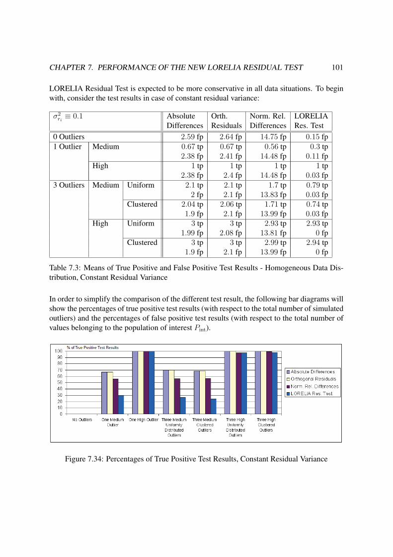
CHAPTER 7. PERFORMANCE OF THE NEW LORELIA RESIDUAL TEST 101
LORELIA Residual Test is expected to be more conservative in all data situations. To begin
with, consider the test results in case of constant residual variance:
σ2ri≡ 0.1 Absolute Orth. Norm. Rel. LORELIA
Differences Residuals Differences Res. Test
0 Outliers 2.59 fp 2.64 fp 14.75 fp 0.15 fp
1 Outlier Medium 0.67 tp 0.67 tp 0.56 tp 0.3 tp
2.38 fp 2.41 fp 14.48 fp 0.11 fp
High 1 tp 1 tp 1 tp 1 tp
2.38 fp 2.4 fp 14.48 fp 0.03 fp
3 Outliers Medium Uniform 2.1 tp 2.1 tp 1.7 tp 0.79 tp
2 fp 2.1 fp 13.83 fp 0.03 fp
Clustered 2.04 tp 2.06 tp 1.71 tp 0.74 tp
1.9 fp 2.1 fp 13.99 fp 0.03 fp
High Uniform 3 tp 3 tp 2.93 tp 2.93 tp
1.99 fp 2.08 fp 13.81 fp 0 fp
Clustered 3 tp 3 tp 2.99 tp 2.94 tp
1.9 fp 2.1 fp 13.99 fp 0 fp
Table 7.3: Means of True Positive and False Positive Test Results - Homogeneous Data Dis-
tribution, Constant Residual Variance
In order to simplify the comparison of the different test result, the following bar diagrams will
show the percentages of true positive test results (with respect to the total number of simulated
outliers) and the percentages of false positive test results (with respect to the total number of
values belonging to the population of interest Pint).
Figure 7.34: Percentages of True Positive Test Results, Constant Residual Variance

CHAPTER 7. PERFORMANCE OF THE NEW LORELIA RESIDUAL TEST 102
Figure 7.35: Percentages of False Positive Test Results, Constant Residual Variance
The following observations can be made:
(i.) A medium outlier term is generally not well identified. A look at the corresponding
plots in Appendix B shows, that a medium outlier is often hidden in the main body of
the data and thus no outlier test will be able to separate this outlier from the normal data.
Therefore, it seems more appropriate to judge the outlier test performances for a higher
outlier term.
(ii.) The fact if the outliers are clustered or uniformly distributed over the measuring range
has no observable influence on the test performances.
(iii.) The performances for the outlier tests based on the absolute differences and on the or-
thogonal residuals are almost identical. This is not astonishing since these tests are
based on the assumption of constant residual variances or constant error variances, re-
spectively, which is approximately equivalent (compare (6.1.5) in Section 6.1). Both
tests deliver appropriate results. The percentages of false positive test results are ap-
proximately constant for every data situation with about 2.5%.
(iv.) The test based on the normalized relative differences is not appropriate in the case of a
constant residual variances. The test delivers too many false positive test results which
are all located in the low concentration range (compare plots in Appendix B).
(v.) The LORELIA Residual Test is more conservative than the test of [Wadsworth, 1990]
based on the absolute differences or on the orthogonal residuals. Remember, that the lo-
cal confidence limits for the LORELIA Residual Test are calculated for a Bonferroni ad-
justed significance level ofαglob
n= 0.1
100= 0.1%, whereas the tests of [Wadsworth, 1990]
are not assigned to a predefined significance level but correspond to very high type 1error rates, compare Table 7.2. Thus, the level of significances of the different outlier
test are not equal. This has to be kept in mind in the comparison of the tests.
For the LORELIA Residual Test, the percentages of true positive test results are espe-
cially low for medium outliers. This can however be explained by (i.). For a high outlier
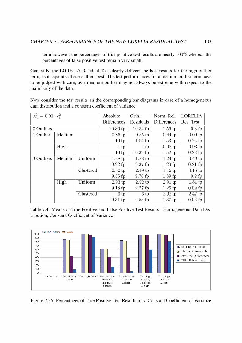
CHAPTER 7. PERFORMANCE OF THE NEW LORELIA RESIDUAL TEST 103
term however, the percentages of true positive test results are nearly 100% whereas the
percentages of false positive test remain very small.
Generally, the LORELIA Residual Test clearly delivers the best results for the high outlier
term, as it separates these outliers best. The test performances for a medium outlier term have
to be judged with care, as a medium outlier may not always be extreme with respect to the
main body of the data.
Now consider the test results an the corresponding bar diagrams in case of a homogeneous
data distribution and a constant coefficient of variance:
σ2ri= 0.01 · c2
i Absolute Orth. Norm. Rel. LORELIA
Differences Residuals Differences Res. Test
0 Outliers 10.36 fp 10.84 fp 1.56 fp 0.3 fp
1 Outlier Medium 0.86 tp 0.85 tp 0.44 tp 0.09 tp
10 fp 10.4 fp 1.53 fp 0.25 fp
High 1 tp 1 tp 0.98 tp 0.93 tp
10 fp 10.39 fp 1.52 fp 0.22 fp
3 Outliers Medium Uniform 1.88 tp 1.88 tp 1.24 tp 0.49 tp
9.22 fp 9.37 fp 1.29 fp 0.21 fp
Clustered 2.52 tp 2.49 tp 1.12 tp 0.15 tp
9.35 fp 9.76 fp 1.39 fp 0.2 fp
High Uniform 2.93 tp 2.92 tp 2.91 tp 1.81 tp
9.18 fp 9.27 fp 1.26 fp 0.09 fp
Clustered 3 tp 3 tp 2.92 tp 2.47 tp
9.31 fp 9.53 fp 1.37 fp 0.06 fp
Table 7.4: Means of True Positive and False Positive Test Results - Homogeneous Data Dis-
tribution, Constant Coefficient of Variance
Figure 7.36: Percentages of True Positive Test Results for a Constant Coefficient of Variance

CHAPTER 7. PERFORMANCE OF THE NEW LORELIA RESIDUAL TEST 104
Figure 7.37: Percentages of False Positive Test Results for a Constant Coefficient of Variance
The above bar diagrams allow the following conclusions:
(i.) The medium outlier term is again not well identified.
(ii.) The outlier tests for the absolute differences and for the orthogonal residuals both deliver
too many false positive test results which are all located at the end of the measuring
range (compare plots in Appendix B) which is explained by the fact that the residual
variances are proportionally increasing for this data model. Although the percentages
of true positive test results are rather high, both test are not appropriate here as the
percentages of false positive test results are of unacceptable magnitude with about 10%for all data situations.
(iii.) The test based on the normalized relative differences is the one of choice in the case of
a constant coefficient of variance. A high outlier term is always well identified. The
percentage of false positive test results is approximately constant for all data situations
with about 1.4%.
(iv.) The LORELIA Residual Test is clearly more conservative than the test based on the
normalized relative differences. The percentages of true positive test results are large
in the case of one high outlier (93%) and in the case of three high clustered outliers
(82, 33%). As the percentages of false positive test results are very low (≤ 0.3%), the
LORELIA Residual Test can be regarded as a more conservative alternative to the test
for the normalized relative differences in these data situations.
(v.) The fact if the outliers are clustered or not seems to influence the percentages of true
positive test results for the LORELIA Residual Test. This first seems astonishing, since
there was no observable influence in the case of a constant residual variance. How-
ever this contradiction can easily be explained. The percentages of true positive test
results are not really influenced by the outlier cluster but by the position of the outliers.

CHAPTER 7. PERFORMANCE OF THE NEW LORELIA RESIDUAL TEST 105
The LORELIA Weighting Function does not involve any model information of the un-
derlying residual variances in order to be globally applicable for every data situation.
Therefore, in the case of a non constant residual variance, the local variance estimates
will be smoothed, especially if the differences between the local residual variances are
large. This means that the local LORELIA Outlier Limits will represent the trend of
the underlying residual variance model, but the local variance estimators will be biased.
The increment of this bias depend on the actual data situation. In the case of a constant
coefficient of variance, the local residual variance will be overestimated at the low con-
centration range and underestimated for higher concentrations. Therefore, outliers at
the low concentration range are less easily detected than at a higher concentration level.
A detailed description of the influence of the outlier position for different data situations
will be given in Section 7.2.
Now, consider the case of a non constant coefficient of variance.
σ2ri= 4 + 0.01 · c2
i Absolute Orth. Norm. Rel. LORELIA
Differences Residuals Differences Res. Test
0 Outliers 7.21 fp 7.25 fp 6.49 fp 0.27 fp
1 Outlier Medium 0.75 tp 0.77 tp 0.23 tp 0.07 tp
6.97 fp 7.09 fp 6.29 fp 0.24 fp
High 1 tp 1 tp 0.92 tp 0.95 tp
6.95 fp 7.06 fp 6.28 fp 0.2 fp
3 Outliers Medium Uniform 1.88 tp 1.78 tp 0.86 tp 0.45 tp
6.43 fp 6.29 fp 6.13 fp 0.18 fp
Clustered 2.2 tp 2.19 tp 0.76 tp 0.17 tp
6.52 fp 6.58 fp 6.08 fp 0.18 fp
High Uniform 2.96 tp 2.94 tp 2.71 tp 1.99 tp
6.43 fp 6.31 fp 6.11 fp 0.09 fp
Clustered 3 tp 3 tp 2.69 tp 2.58 tp
6.5 fp 6.51 fp 6.06 fp 0.06 fp
Table 7.5: Homogeneous Data Distribution, Non Constant Coefficient of Variance
The percentages of true positive and false positive test results are given by:

CHAPTER 7. PERFORMANCE OF THE NEW LORELIA RESIDUAL TEST 106
Figure 7.38: Percentages of True Positive Test Results, Non Constant Coefficient of Variance
Figure 7.39: Means of True Positive and False Positive Test Results - Homogeneous Data
Distribution, Non Constant Coefficient of Variance
The following observations are made:
(i.) The medium outlier term is not well identified.
(ii.) The outlier tests for the absolute differences and for the orthogonal residuals both deliver
too many false positive test results which are all located at the end of the measuring
range (compare plots in Appendix B) which is explained by the fact that the residual
variances are increasing. Although, the percentages of true positive test results are rather
high, both test are not appropriate here as the percentages of false positive test results
are unacceptable large with about 6.6%− 7.2% for all data situations.
(iii.) The test based on the normalized relative differences deliver too many false positive test
results which are all located at the low concentration range (compare plots in Appendix

CHAPTER 7. PERFORMANCE OF THE NEW LORELIA RESIDUAL TEST 107
B) which is explained by the fact that the coefficient of variances is not constant here.
Despite the high percentages of true positive test results, both test are not appropriate
here as the percentages of false positive test results are unacceptable high with about
6.3% for all data situations.
(iv.) The LORELIA Residual Test delivers the only appropriate results, with respect to the
percentages of false positive test results. Again it can be observed that the LORELIA
Residual test is more conservative than all other tests. The percentage of true positive
test results is maximal for the case of one high outlier term with 95%.
(v.) Again, the percentages of true positive test results are influenced by the position of the
outliers which will be discussed in detail in Section 7.2.
7.1.3.3 General Observations and Conclusions
A performance ranking based on the number of true positive and false positive test results is
given in the following table:
Residual Absolute Orth. Norm. Rel. LORELIA
Variance Differences Residuals Differences Res. Test
Constant Highly appropriate, Not appropriate, Highly appropriate,
no adjustment of too many false Bonferroni adjusted
the local positive test results confidence limits
significance levels, at the low
thus too sensitive concentration range
Constant CV Not appropriate, Highly appropriate, Appropriate,
too many false no adjustment of performance depends
positive test results the local on the outlier position
at the high significance levels, and on the amount of
concentration range thus too sensitive the increment between the
local residual variances
Bonferroni adjusted
confidence limits
Non Constant CV Not appropriate, Not appropriate, Appropriate,
too many false too many false performance depends
positive test results positive test results on the outlier position
at the high at the low and on the amount of
concentration range concentration range the increment between the
local residual variances
Bonferroni adjusted
confidence limits
Table 7.6: Performance Ranking

CHAPTER 7. PERFORMANCE OF THE NEW LORELIA RESIDUAL TEST 108
Beside the above performance ranking, a look at the plots (regression plot, scatter plot/residual
plot) can reveal supplementary information on the behavior of the different tests, which will
be resumed and discussed in the following:
(i.) Generally, the high outlier term is a lot better identified by all tests than the medium
outlier term which is often hidden in the main body of the data.
(ii.) The fact if the outliers are uniformly distributed or clustered for a total number of three
outliers does not seem to have an observable influence on the test outputs. This is ex-
plained by the fact that all test are constructed to be robust against outliers, the LORE-
LIA Residual Test involves a reliability measure in the residual variance estimator, all
other tests are based on the median absolute deviation as a robust measure.
(iii.) Note that the position of the outliers within the dataset does have an important influence
for the LORELIA Residual Test which can be mainly observed for simulated datasets
with three uniformly distributed outliers. The question how the outlier position influ-
ences outlier identification for the LORELIA Residual Test will be explored in detail in
Section 7.2.
(iv.) In case of a non constant residual variance, the performance of the LORELIA Residual
test clearly depends on the fact how well the local residual variances are estimated. For
a constant coefficient of variance, the residual variances are underestimated for higher
concentrated samples and overestimated at the low concentration range. Thus, outliers
in the higher concentration range may therefore not be identified:
Figure 7.40: Homogeneous Data Distribution, Constant Coefficient of Variance, Three Out-
liers, Medium Outlier Term, Uniformly Distributed Outliers
(v.) The LORELIA Residual Test is the only test with an adjusted level of significance for
the multiple testing situation, which is clearly a drawback of all other tests. Thus, the
LORELIA Residual test is more conservative than all other tests, compare Table 7.2.

CHAPTER 7. PERFORMANCE OF THE NEW LORELIA RESIDUAL TEST 109
The residual plots often reveal that a non identified outlier lays just slightly inside its
corresponding confidence limit and may be detected when tested with a higher level of
significance or a less conservative adjustment procedure than Bonferroni’s.
Figure 7.41: Homogeneous Data Distribution, Constant Residual Variance, Three Outliers,
Medium Outlier Term, Clustered Outliers
Generally, if the normal assumption for the comparison measure under consideration is met
and the sample distribution within the measuring range is homogeneous, the test proposed
by [Wadsworth, 1990] delivers appropriate results and is fast and easy to calculate. However
these assumptions are often not fulfilled and an appropriate data transformation is not always
easy to find. Although there exist a variety of transformation methods proposed in the sta-
tistical literature, compare for example [Hawkins, 1980], there still exist data situations for
which none of the transformation methods will fit. Moreover in practical applications, the
data analysts are often non statisticians who are not very experienced in this field and who
often fail to judge the underlying distribution and thus to find an appropriate transformation
rule. The LORELIA Residual Test has the clear advantage, that it is globally applicable to
any data situation. No statistical assumptions on the underlying error variances have to be
checked and no data transformations are needed. The residual plot including the local outlier
limits reveals the trend of the underlying residual variance model even to non statisticians.
7.2 Influence of the Outlier Position on its Identification
In this section, the influence of the outlier position within the dataset on its identification is
analyzed for different representative data situations by a simulation study. The LORELIA
Residual Test is used on simulated datasets containing one outlier. The position of this outlier
within the dataset is varied over the entire measuring range. The aim is to generate a functional
relation between the outlier position and the expected percentage of true positive test results.
The underlying simulation plan will be given in the following section.
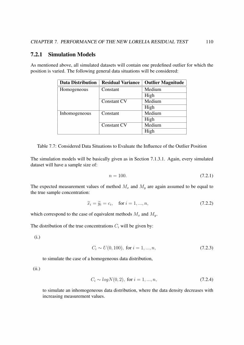
CHAPTER 7. PERFORMANCE OF THE NEW LORELIA RESIDUAL TEST 110
7.2.1 Simulation Models
As mentioned above, all simulated datasets will contain one predefined outlier for which the
position is varied. The following general data situations will be considered:
Data Distribution Residual Variance Outlier MagnitudeHomogeneous Constant Medium
High
Constant CV Medium
High
Inhomogeneous Constant Medium
High
Constant CV Medium
High
Table 7.7: Considered Data Situations to Evaluate the Influence of the Outlier Position
The simulation models will be basically given as in Section 7.1.3.1. Again, every simulated
dataset will have a sample size of:
n = 100. (7.2.1)
The expected measurement values of method Mx and My are again assumed to be equal to
the true sample concentration:
xi = yi = ci, for i = 1, ..., n, (7.2.2)
which correspond to the case of equivalent methods Mx and My.
The distribution of the true concentrations Ci will be given by:
(i.)
Ci ∼ U(0, 100), for i = 1, ..., n, (7.2.3)
to simulate the case of a homogeneous data distribution,
(ii.)
Ci ∼ logN(0, 2), for i = 1, ..., n, (7.2.4)
to simulate an inhomogeneous data distribution, where the data density decreases with
increasing measurement values.
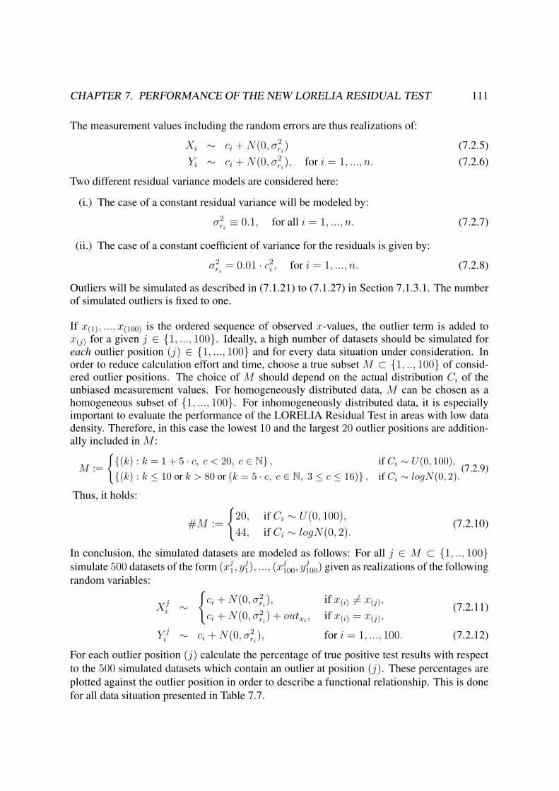
CHAPTER 7. PERFORMANCE OF THE NEW LORELIA RESIDUAL TEST 111
The measurement values including the random errors are thus realizations of:
Xi ∼ ci +N(0, σ2ri) (7.2.5)
Yi ∼ ci +N(0, σ2ri), for i = 1, ..., n. (7.2.6)
Two different residual variance models are considered here:
(i.) The case of a constant residual variance will be modeled by:
σ2ri≡ 0.1, for all i = 1, ..., n. (7.2.7)
(ii.) The case of a constant coefficient of variance for the residuals is given by:
σ2ri= 0.01 · c2
i , for i = 1, ..., n. (7.2.8)
Outliers will be simulated as described in (7.1.21) to (7.1.27) in Section 7.1.3.1. The numberof simulated outliers is fixed to one.
If x(1), ..., x(100) is the ordered sequence of observed x-values, the outlier term is added tox(j) for a given j ∈ {1, ..., 100}. Ideally, a high number of datasets should be simulated foreach outlier position (j) ∈ {1, ..., 100} and for every data situation under consideration. Inorder to reduce calculation effort and time, choose a true subset M ⊂ {1, .., 100} of consid-ered outlier positions. The choice of M should depend on the actual distribution Ci of theunbiased measurement values. For homogeneously distributed data, M can be chosen as ahomogeneous subset of {1, ..., 100}. For inhomogeneously distributed data, it is especiallyimportant to evaluate the performance of the LORELIA Residual Test in areas with low datadensity. Therefore, in this case the lowest 10 and the largest 20 outlier positions are addition-ally included in M :
M :=
{{(k) : k = 1 + 5 · c, c < 20, c ∈ N} , if Ci ∼ U(0, 100),{(k) : k ≤ 10 or k > 80 or (k = 5 · c, c ∈ N, 3 ≤ c ≤ 16)} , if Ci ∼ logN(0, 2).
(7.2.9)
Thus, it holds:
#M :=
{20, if Ci ∼ U(0, 100),
44, if Ci ∼ logN(0, 2).(7.2.10)
In conclusion, the simulated datasets are modeled as follows: For all j ∈ M ⊂ {1, .., 100}simulate 500 datasets of the form (xj
1, yj1), ..., (x
j100, y
j100) given as realizations of the following
random variables:
Xji ∼
{ci +N(0, σ2
ri), if x(i) �= x(j),
ci +N(0, σ2ri) + outxi
, if x(i) = x(j),(7.2.11)
Y ji ∼ ci +N(0, σ2
ri), for i = 1, ..., 100. (7.2.12)
For each outlier position (j) calculate the percentage of true positive test results with respect
to the 500 simulated datasets which contain an outlier at position (j). These percentages are
plotted against the outlier position in order to describe a functional relationship. This is done
for all data situation presented in Table 7.7.

CHAPTER 7. PERFORMANCE OF THE NEW LORELIA RESIDUAL TEST 112
7.2.2 Homogeneous Data Distribution
To begin with, consider the case of a homogeneous data distribution (7.2.3) for a constant
residual variance (7.2.7) or a constant coefficient of variance (7.2.8) with a medium outlier
term (7.1.26) or a high outlier term (7.1.27), respectively.
7.2.2.1 Constant Residual Variance
In this section, the most simplest case of a homogeneous data distribution for a constant
residual variance is evaluated. To begin with, the expected results will be mathematically
estimated and discussed. In the following, these expected results will be compared to the
observed simulation results.
7.2.2.1.1 Expected Results
In the following, the local confidence limits Cαloc,i will be approximated analytically for the
special case of a homogeneous data distribution and a constant residual variance. The follow-
ing theorem will be used for the approximation:
Theorem 7.4Consider the case of a constant residual variance:
Riiid∼ N(0, σ2
r), for i = 1, ..., n. (7.2.13)
Assume further that the following assumption for the reliability measure Γk,n is fulfilled (com-pare definition (6.5) in Section 6.4):
Γk,n = 1, for all k = 1, ..., n. (7.2.14)
In this case the LORELIA Residual Variance Estimator given in Definition 6.7 in Section 6.5is an unbiased estimator of the true residual variance σ2
r .
Proof: The LORELIA Residual Variance estimator is given by:
σ2ri=
1∑nl=1 wil
·n∑
k=1
wik · r2k =
1∑nl=1Δil · Γl,n
·n∑
k=1
Δik · Γk,n · r2k, for i = 1, ..., n.
Note that, by Definition (6.2) in Section 6.4, the distance measure Δik is statistically indepen-
dent of the random variable R2k, as the distance between the orthogonal projection does not
depend on the actual values of the residuals. The reliability measure Γk,n defined in (6.5) how-
ever is statistically dependent of R2k. In the following it will therefore be denoted by Γk,n (R
2k).

CHAPTER 7. PERFORMANCE OF THE NEW LORELIA RESIDUAL TEST 113
It holds:
E(σ2
ri
)= E
⎛⎜⎜⎜⎝ 1∑nl=1Δil · Γl,n(R
2k)︸ ︷︷ ︸
=1, by (7.2.14)
·n∑
k=1
Δik · Γk,n(R2k)︸ ︷︷ ︸
=1, by (7.2.14)
·R2k
⎞⎟⎟⎟⎠= E
(1∑n
l=1Δil
·n∑
k=1
Δik ·R2k
)
=1∑n
l=1Δil
·n∑
k=1
Δik · E(R2
k
)= E
(R2) · 1∑n
l=1Δil
·n∑
k=1
Δik
= E(R2)− E(R)2︸ ︷︷ ︸=0, by (7.2.13)
= V ar(R) = σ2r .
Thus, the LORELIA residual variance estimator is unbiased in the case of a constant residual
variance σ2r if the reliability measure Γk,n(R
2k) equals 1.
Remark 7.5If the residual variances are assumed to be constant over the measuring range and no outliers
are present, then γk,n defined in (6.4.9) in Section 6.4.2 is approximately given by 1n
for all
k = 1, ..., n and thus Γk,n ≈ 1 which motivates assumption (7.2.14) in Theorem 7.4.
The local outlier limits are calculated as (1−αloc)% approximative confidence intervals Cαloc,i
for i = 1, ..., n. In order to give a rough estimate of the expected percentage of true positive
test results, these local confidence intervals will be approximated for every i = 1, ..., n by:
Cαloc,i := [−tDFi,(1−αloc2
) · σri, tDFi,(1−αloc
2) · σri
]
≈ [−z(1−αloc2
) · σr, z(1−αloc2
) · σr]. (7.2.15)
where z(1−αloc2
) is the (1− αloc
2)% quantile of the standard normal distribution.
Now, the distributional properties of an outlier residual Ri are deduced. Remember, that
an outlier at position (j) is simulated as:
X(j) ∼ c(j) +N(0, σ2r) + outx(j)
= c(j) +N(outx(j), σ2
r),
Y(j) ∼ c(j) +N(0, σ2r).
For visualization, consider the following plot:

CHAPTER 7. PERFORMANCE OF THE NEW LORELIA RESIDUAL TEST 114
Figure 7.42: The Outlier Residual
By the Pythagorean Theorem the outlying residual is thus a realizations of:
R(j) ∼ 1√2
(N(outx(j)
, σ2r)−N(0, σ2
r))
=1√2N(outx(j)
, 2 · σ2r)
= N
(outx(j)√
2, σ2
r
)= N
(k · σr√
2, σ2
r
)=
k · σr√2
+N(0, σ2
r
). (7.2.16)
Hence, it holds:
P(R(j) > z(1−αloc
2) · σr
)= P
(k · σr√
2+N
(0, σ2
r
)> z(1−αloc
2) · σr
)= P
(N(0, σ2
r
)> z(1−αloc
2) · σr − k · σr√
2
)= P
(N(0, 1) > z(1−αloc
2) −
k√2
). (7.2.17)
For αglob = 0.1 and a sample size of n = 100, the Bonferroni adjusted local significance level
is given by αloc = 0.001. Therefore it follows:
P(R(j) > z(1−αloc
2) · σr
)= P
(N(0, 1) > z0.9995 − k√
2
)≈{
P (N(0, 1) > 0.46) ≈ 0.32, for k = 4,
P (N(0, 1) > −2.37) ≈ 0.99, for k = 8.(7.2.18)

CHAPTER 7. PERFORMANCE OF THE NEW LORELIA RESIDUAL TEST 115
Remark 7.6Note that the above calculation can only be considered as a rough estimate for the expected
results. On the one hand, an outlying residual does not fulfill the assumptions (7.2.13) and
(7.2.14) in Theorem 7.4, as the outlying residual follow the distribution given in (7.2.16) and
will have a reliability weight which is much smaller than 1. However if only one outlier
is present, this problem may be neglected since the outlying measurement is ideally down
weighted to an amount of 0 and thus does not bias the residual variance estimator much.
On the other hand, the approximation of the Students-t by the normal quantiles is prob-
lematical, as the Students-t quantiles correspond to different degrees of freedom for every
i = 1, ..., n. By (6.5.5), the degrees of freedom are given by:
DFi =(∑n
k=1 wik · r2k)
2∑nk=1 w2
ik · r4k
, for i = 1, ..., n,
which is an increasing function of the sum of weights∑n
k=1 wik. As the weights are based
on a continuous distance measure and the data distribution is assumed to be homogeneous,
the sum of weights will be maximal for a local residual variance estimate in the middle of
the measuring range as the the distances to the neighbored residuals will be the shortest. This
will lead to outlier limits which are wider on the borders than in the middle of the measuring
range. Thus outliers are expected to be better identified in the middle of the measuring range
where the information density is higher than on the borders.
7.2.2.1.2 Observed Results
For a medium outlier term which correspond to outxi= 4 · σr, compare (7.1.26), the plot
of the percentages of true positive test results for each outlier position (j) ∈M is given by:
Figure 7.43: Relation between Outlier Position and Percentages of True Positive Test Results
- Homogeneous Data Distribution, Constant Residual Variance, Medium Outlier Term

CHAPTER 7. PERFORMANCE OF THE NEW LORELIA RESIDUAL TEST 116
To compare these observed results with the expected results given in (7.2.18) in the previous
section, consider the corresponding descriptive analysis:
Quantiles Moments100% Maximum 34.4 Mean 29.9
75% Quartile 31.55 Standard Deviation 2.94
50% Median 30.5 Standard Error for the Mean 0.66
25% Quartile 28.4 Upper 95% Limit for the Mean 31.27
0% Minimum 22 Lower 95% Limit for the Mean 28.53
Sample Size 20
Table 7.8: Descriptive Analysis for Percentages of True Positive Test Results - Homogeneous
Data Distribution, Constant Residual Variance, Medium Outlier Term
The calculated mean and median for the percentages of true positive test results given by
29.9% and 30.5%, respectively, are close to the expected value of 32% given in (7.2.18).
However by Remark 7.6, the above descriptive analysis can only give a rough overview of
the simulation results, as the percentages of true positive test results are not expected to be
constant over all outlier positions. This also causes the high standard deviation given by
2.94%. If the above plot is zoomed in, it will become obvious that the percentage of true
positive test results is higher in the middle of the measuring range than on the borders. To
visualize this, a polynomial of degree 2 is fit in the plot:
Figure 7.44: Polynomial Fit for Percentages of True Positive Test Results - Homogeneous
Data Distribution, Constant Residual Variance, Medium Outlier Term

CHAPTER 7. PERFORMANCE OF THE NEW LORELIA RESIDUAL TEST 117
Now, the functional relation between the outlier position an the percentages of true positive
test results is shown for the case of a high outlier term given by outxi= 8 · σr which corre-
sponds to (7.1.27).
Figure 7.45: Relation between Outlier Position and Percentages of True Positive Test Results
- Homogeneous Data Distribution, Constant Residual Variance, High Outlier Term
For the comparison to the expected results consider the corresponding descriptive analysis:
Quantiles Moments100% Maximum 99.8 Mean 98.92
75% Quartile 99.4 Standard Deviation 0.74
50% Median 99.1 Standard Error for the Mean 0.17
25% Quartile 98.65 Upper 95% Limit for the Mean 99.27
0% Minimum 96.6 Lower 95% Limit for the Mean 98.57
Sample Size 20
Table 7.9: Descriptive Analysis for Percentages of True Positive Test Results - Homogeneous
Data Distribution, Constant Residual Variance, High Outlier Term
The mean and the median given by 98.92% respective 99.1% are very similar to the expected
result of 99% given in (7.2.18). The standard deviation is very low here with 0.74%. This is
explained by the fact that a high outlier term corresponds to a very extreme outlier which will
nearly always be detected. As the percentage of true positive test results is almost 100% for all
outlier positions, the influence of the different local degrees of freedom can thus be neglected
here.

CHAPTER 7. PERFORMANCE OF THE NEW LORELIA RESIDUAL TEST 118
In conclusion, the following general observations can be made:
(i.) In the case of a homogeneous data distribution and a constant residual variance, outliers
are well identified by the LORELIA Residual if the outlier is well separated from the
main body of the data.
(ii.) For an outlier term between 4 · σr and 8 · σr, the percentages of true positive test results
lay approximatively within [30%, 100%].
(iii.) The variation between the percentages of true positive test results for different outlier
positions decreases for an increasing outlier term.
7.2.2.2 Constant Coefficient of Variance
Now, the case of a constant coefficient of variance will be considered which is simulated as
described in (7.2.8). As the behavior of the LORELIA Residual Variance estimator is much
more complex in this case, the expected results can not be explicitly calculated anymore.
However in the following section, the expected trends will be discussed based on theoretical
considerations.
7.2.2.2.1 Expected Results
The LORELIA Weighting Method does not involve any model information of the underly-
ing residual variances in order to be globally applicable for every data situation. Therefore, in
the case of a non constant residual variance, the local variance estimates will be smoothed as
already mentioned in Section 7.1.3.2. The local LORELIA Outlier Limits will well represent
the trend of the underlying residual variance model, but the corresponding variance estimates
will be biased. In the case of a constant coefficient of variance, the local residual variance will
be overestimated at the low concentration range and underestimated for higher concentrations.
Therefore, outliers at the low concentration range are less easily detected than outliers corre-
sponding to higher concentrations. Thus, a monotonously increasing functional relationship
between the outlier position and the percentages of true positive test results is expected.
7.2.2.2.2 Observed Results
To begin with, consider the case of a medium outlier term. As expected, the percentage of true
positive test results is an increasing function of the outlier position. At a low concentration
level, the medium outlier term is never identified, whereas for the highest concentration the
percentage of true positive test results reaches nearly 70%:

CHAPTER 7. PERFORMANCE OF THE NEW LORELIA RESIDUAL TEST 119
Figure 7.46: Relation between Outlier Position and Percentages of True Positive Test Results
- Homogeneous Data Distribution, Constant Coefficient of Variance, Medium Outlier Term
For a high outlier term, the same expected trend can be observed. However, the outlier identi-
fication fails completely only for very low concentrations. The percentage of true positive test
results increases very soon up to 100%.
Figure 7.47: Relation between Outlier Position and Percentages of True Positive Test Results
- Homogeneous Data Distribution, Constant Coefficient of Variance, High Outlier Term
For the case of a homogeneous data distribution with a constant coefficient of variance, the
following general conclusions can be drawn:
(i.) The percentage of true positive test results is an increasing function of the outlier po-

CHAPTER 7. PERFORMANCE OF THE NEW LORELIA RESIDUAL TEST 120
sition. The magnitude of this increment depends on the underlying amount of change
between the local residual variances. The function becomes steeper if the outlier term
increases.
(ii.) Outliers for low concentrated samples are not (well) identified. For an outlier term given
by 4 · σr, the LORELIA Residual Test fails completely in nearly 1/3 of the measuring
range. For an outlier term of 8 · σr however, the outlier identification fails only in the
lowest 1/10 of the measuring range.
(iii.) If the outlier term is given by 8 · σr, the percentage of true positive test results is about
100% in the upper half of the measuring range.
7.2.3 Inhomogeneous Data Distribution
Now, the case of an inhomogeneous sample distribution (7.2.4) will be considered to evaluate
the influence of the local data density on the test performance.
Thereby, note that the outlier position is a relative measure for the outlier location with respect
to the ordered sequence of x-values. In the case of a homogeneous sample distribution, the
relative position of the outlier corresponds well to the absolute location of the outlier within
the measuring range. In the case of an inhomogeneous data distribution however, the outlier
position does not match with the absolute location of the outlier within the measuring range.
In order to describe the functional relationship between the absolute location of the outliers
and the percentage of true positive test results, an additional plot is needed. In a first step, the
measuring range is split into intervals of length 0.5. The x-component of every simulated out-
lier lays exactly within one of these intervals. Now, count the number of outliers within each
interval over all simulated datasets. For every interval, the percentage of identified outliers
with respect to the total number of outliers located in this interval is calculated. The percent-
ages of true positive test results can thus be plotted as a step function of the simulated outlier
x-components. The range of considered outlier x-components is reduced to [2.5, 25] here, as
for the given simulation settings only some isolated outliers had x-components outside this
range.
Note, that the percentages of true positive test results within each interval are based on very
different sample sizes, as the total number of outliers located in each interval decreases with
decreasing data density. Therefore, the scattering of the true positive test results will increase
with increasing x-components. To overcome this confounding aspect, a polynomial of degree
6 is fit additionally to clearly visualize the functional trend.
7.2.3.1 Constant Residual Variance
In the case of a constant residual variance, the influence of the outlier position on the test
performance will be mainly determined by the effect of inhomogeneous local data densities

CHAPTER 7. PERFORMANCE OF THE NEW LORELIA RESIDUAL TEST 121
(compare the results of Section 7.2.2.1). The expected results are discussed in the following
section.
7.2.3.1.1 Expected Results
For a low local data density, the sum of weights∑n
k=1 wik for a residual ri located in this
data area will be small, since all distance weights Δik with k �= i will be low. By Remark 7.6,
the degrees of freedom DFi are an increasing function of the sum of weights. Thus, outlier
limits will be wider in areas with low local data density than in areas with a high data density.
Therefore, outliers will be best identified if the local data density is maximal. As the inhomo-
geneous data distribution is modeled with a log normal distribution, the local data density is
low for high concentrations. The data density will be maximal for small concentrations. Note
that for very small concentrations near 0, the local data density will decrease, as well.
7.2.3.1.2 Observed Results
For a medium outlier term, the expected trend is well met.
Figure 7.48: Relation between Outlier Position and Percentages of True Positive Test Results
- Inhomogeneous Data Distribution, Constant Residual Variance, Medium Outlier Term
The percentages of true positive test results first increase until a maximum is reached. This
maximum corresponds to the maximal local data density located at the left border of the mea-
suring range. For increasing concentrations, the local data density decreases and thus the
percentage of true positive test results decreases, as well.
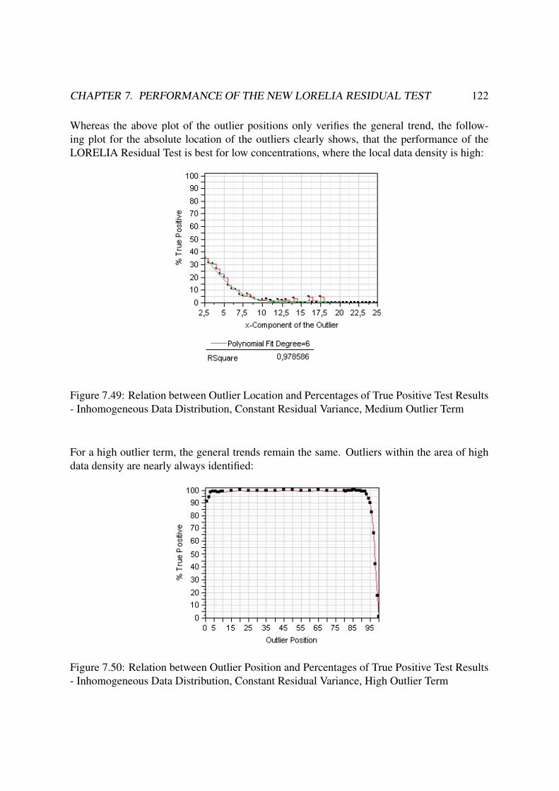
CHAPTER 7. PERFORMANCE OF THE NEW LORELIA RESIDUAL TEST 122
Whereas the above plot of the outlier positions only verifies the general trend, the follow-
ing plot for the absolute location of the outliers clearly shows, that the performance of the
LORELIA Residual Test is best for low concentrations, where the local data density is high:
Figure 7.49: Relation between Outlier Location and Percentages of True Positive Test Results
- Inhomogeneous Data Distribution, Constant Residual Variance, Medium Outlier Term
For a high outlier term, the general trends remain the same. Outliers within the area of high
data density are nearly always identified:
Figure 7.50: Relation between Outlier Position and Percentages of True Positive Test Results
- Inhomogeneous Data Distribution, Constant Residual Variance, High Outlier Term

CHAPTER 7. PERFORMANCE OF THE NEW LORELIA RESIDUAL TEST 123
Figure 7.51: Relation between Outlier Location and Percentages of True Positive Test Results
- Inhomogeneous Data Distribution, Constant Residual Variance, High Outlier Term
In the case of an inhomogeneous data distribution with a constant residual variance, the fol-
lowing general observations can be made:
(i.) The percentage of true positive test results increases with increasing data density.
(ii.) For a high outlier term given by 8 ·σr, the percentage of true positive test results is about
100% in the area with the maximal local data density, but decreases down to 0% for the
minimal local data density at the right end of the measuring range.
7.2.3.2 Constant Coefficient of Variance
Now, an inhomogeneous sample distribution is considered for the case of a constant coefficient
of residual variances.
7.2.3.2.1 Expected Results
If the data distribution is inhomogeneous and a constant coefficient of variance is given, the
effects discussed in Section 7.2.2.2 and 7.2.3.1 will be mixed. On the one hand, the perfor-
mance of the outlier test is influenced by the underlying residual variance model, which leads
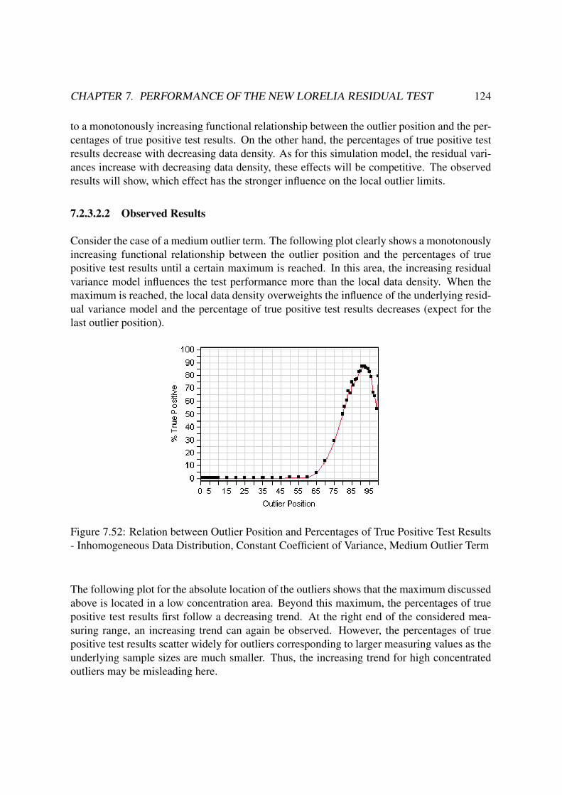
CHAPTER 7. PERFORMANCE OF THE NEW LORELIA RESIDUAL TEST 124
to a monotonously increasing functional relationship between the outlier position and the per-
centages of true positive test results. On the other hand, the percentages of true positive test
results decrease with decreasing data density. As for this simulation model, the residual vari-
ances increase with decreasing data density, these effects will be competitive. The observed
results will show, which effect has the stronger influence on the local outlier limits.
7.2.3.2.2 Observed Results
Consider the case of a medium outlier term. The following plot clearly shows a monotonously
increasing functional relationship between the outlier position and the percentages of true
positive test results until a certain maximum is reached. In this area, the increasing residual
variance model influences the test performance more than the local data density. When the
maximum is reached, the local data density overweights the influence of the underlying resid-
ual variance model and the percentage of true positive test results decreases (expect for the
last outlier position).
Figure 7.52: Relation between Outlier Position and Percentages of True Positive Test Results
- Inhomogeneous Data Distribution, Constant Coefficient of Variance, Medium Outlier Term
The following plot for the absolute location of the outliers shows that the maximum discussed
above is located in a low concentration area. Beyond this maximum, the percentages of true
positive test results first follow a decreasing trend. At the right end of the considered mea-
suring range, an increasing trend can again be observed. However, the percentages of true
positive test results scatter widely for outliers corresponding to larger measuring values as the
underlying sample sizes are much smaller. Thus, the increasing trend for high concentrated
outliers may be misleading here.

CHAPTER 7. PERFORMANCE OF THE NEW LORELIA RESIDUAL TEST 125
Figure 7.53: Relation between Outlier Location and Percentages of True Positive Test Results
- Histogram, Inhomogeneous Data Distribution, Constant Coefficient of Variance, Medium
Outlier Term
Similar but more extreme observations as in Figure 7.52 and 7.53 can be made in the case of
a high outlier term:
Figure 7.54: Relation between Outlier Position and Percentages of True Positive Test Results
- Inhomogeneous Data Distribution, Constant Coefficient of Variance, High Outlier Term

CHAPTER 7. PERFORMANCE OF THE NEW LORELIA RESIDUAL TEST 126
Figure 7.55: Relation between Outlier Location and Percentages of True Positive Test Re-
sults - Histogram, Inhomogeneous Data Distribution, Constant Coefficient of Variance, High
Outlier Term
Generally, for an inhomogeneous data distribution with a constant coefficient of variance, the
functional relationship between the outlier position and the percentage of true positive test
results will be a mixture of the functional trends described in Section 7.2.2.2 and 7.2.3.1. The
influence balance between the local data density and the underlying residual variance model
will depend on the given distributions and parameter settings and thus a functional trend can
not generally be described.
7.3 How to Deal with Complex Residual Variance Models
If the local residual variances change too drastically over the measuring range, the perfor-
mance of the LORELIA Residual Test is very poor. In this section, a discussion on the above
problem and a suggestion how to deal with it is given.
If the local residual variances within a dataset are of very different magnitude or the under-
lying residual variance model is very complex, the LORELIA Residual Variance Estimates
may be heavily biased. Therefore, the user of the LORELIA Residual Test is strongly rec-
ommended to have a look at the corresponding residual plot to verify visually if the local
confidence limits seem appropriate and if obvious outlier candidates are well identified. If
this is not the case, it may help to split the dataset in order to reduce the complexity of the
residual variance model. The following example will illustrate the problem:

CHAPTER 7. PERFORMANCE OF THE NEW LORELIA RESIDUAL TEST 127
Figure 7.56: Exemplary Dataset - Bad Performance of the LORELIA Residual Test
A cloud of outliers is identified at the low concentration limit. The local outlier limits do not
merge smoothly. The reliability plot shows, that a huge number of residuals is down weighted
to an amount of 0. These residuals are thus excluded from the calculation of all residual
variance estimates:
Figure 7.57: Exemplary Dataset - Reliability Plot
The above effect occurs for the following reasons: The sample size is very large with n = 774.
The sample distribution within the measuring range is very inhomogeneous - about 94% of
the measurement values lay within the first hundredth of the measuring range. Moreover, the
residual variances are increasing over the measuring range. Thus, the residuals corresponding
to the few high concentrated measurement values nearly all are assigned to a reliability weight
of 0.

CHAPTER 7. PERFORMANCE OF THE NEW LORELIA RESIDUAL TEST 128
Now, the dataset is split. For the low part of the dataset corresponding to the first 726measure-
ment values, the local residual variances turn out to be nearly constant. One obvious outlier is
clearly identified:
Figure 7.58: Exemplary Dataset, Low Part - Improved Performance
Most residuals correspond to a reliability weight close to 1. Only the identified outlier is down
weighted to an amount of 0:
Figure 7.59: Exemplary Dataset, Low Part - Reliability Plot
For the upper part of the dataset, the local residual variances are increasing. No outliers are
identified. The local outlier limits merge smoothly:

CHAPTER 7. PERFORMANCE OF THE NEW LORELIA RESIDUAL TEST 129
Figure 7.60: Exemplary Dataset, Upper Part - Improved Performance
The reliability plots reveals one value which is down weighted to 0. A look at the residual
plot shows that this value lays just slightly within its corresponding confidence interval.
Figure 7.61: Exemplary Dataset, High Part - Reliability Plot
The above example shows, that an appropriate split of the dataset can improve the performance
of the LORELIA Residual Test. As the splitting of the dataset implies that two separate outlier
tests are performed, the global significance level αglob corresponds no longer to the entire
dataset but to the two reduced datasets.
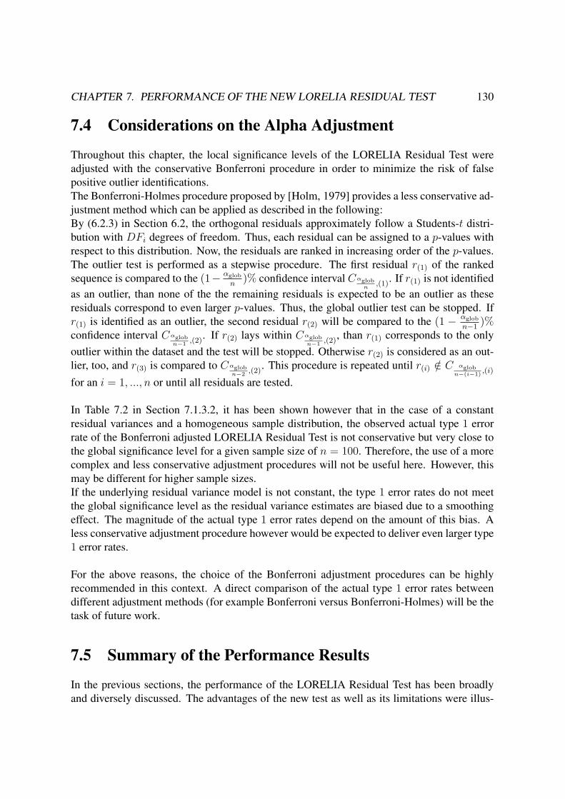
CHAPTER 7. PERFORMANCE OF THE NEW LORELIA RESIDUAL TEST 130
7.4 Considerations on the Alpha Adjustment
Throughout this chapter, the local significance levels of the LORELIA Residual Test were
adjusted with the conservative Bonferroni procedure in order to minimize the risk of false
positive outlier identifications.
The Bonferroni-Holmes procedure proposed by [Holm, 1979] provides a less conservative ad-
justment method which can be applied as described in the following:
By (6.2.3) in Section 6.2, the orthogonal residuals approximately follow a Students-t distri-
bution with DFi degrees of freedom. Thus, each residual can be assigned to a p-values with
respect to this distribution. Now, the residuals are ranked in increasing order of the p-values.
The outlier test is performed as a stepwise procedure. The first residual r(1) of the ranked
sequence is compared to the (1− αglob
n)% confidence interval Cαglob
n,(1)
. If r(1) is not identified
as an outlier, than none of the the remaining residuals is expected to be an outlier as these
residuals correspond to even larger p-values. Thus, the global outlier test can be stopped. If
r(1) is identified as an outlier, the second residual r(2) will be compared to the (1 − αglob
n−1)%
confidence interval Cαglobn−1
,(2). If r(2) lays within Cαglob
n−1,(2)
, than r(1) corresponds to the only
outlier within the dataset and the test will be stopped. Otherwise r(2) is considered as an out-
lier, too, and r(3) is compared to Cαglobn−2
,(2). This procedure is repeated until r(i) /∈ C αglob
n−(i−1),(i)
for an i = 1, ..., n or until all residuals are tested.
In Table 7.2 in Section 7.1.3.2, it has been shown however that in the case of a constant
residual variances and a homogeneous sample distribution, the observed actual type 1 error
rate of the Bonferroni adjusted LORELIA Residual Test is not conservative but very close to
the global significance level for a given sample size of n = 100. Therefore, the use of a more
complex and less conservative adjustment procedures will not be useful here. However, this
may be different for higher sample sizes.
If the underlying residual variance model is not constant, the type 1 error rates do not meet
the global significance level as the residual variance estimates are biased due to a smoothing
effect. The magnitude of the actual type 1 error rates depend on the amount of this bias. A
less conservative adjustment procedure however would be expected to deliver even larger type
1 error rates.
For the above reasons, the choice of the Bonferroni adjustment procedures can be highly
recommended in this context. A direct comparison of the actual type 1 error rates between
different adjustment methods (for example Bonferroni versus Bonferroni-Holmes) will be the
task of future work.
7.5 Summary of the Performance Results
In the previous sections, the performance of the LORELIA Residual Test has been broadly
and diversely discussed. The advantages of the new test as well as its limitations were illus-
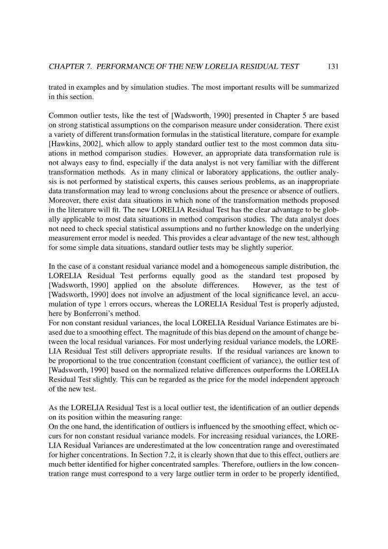
CHAPTER 7. PERFORMANCE OF THE NEW LORELIA RESIDUAL TEST 131
trated in examples and by simulation studies. The most important results will be summarized
in this section.
Common outlier tests, like the test of [Wadsworth, 1990] presented in Chapter 5 are based
on strong statistical assumptions on the comparison measure under consideration. There exist
a variety of different transformation formulas in the statistical literature, compare for example
[Hawkins, 2002], which allow to apply standard outlier test to the most common data situ-
ations in method comparison studies. However, an appropriate data transformation rule is
not always easy to find, especially if the data analyst is not very familiar with the different
transformation methods. As in many clinical or laboratory applications, the outlier analy-
sis is not performed by statistical experts, this causes serious problems, as an inappropriate
data transformation may lead to wrong conclusions about the presence or absence of outliers.
Moreover, there exist data situations in which none of the transformation methods proposed
in the literature will fit. The new LORELIA Residual Test has the clear advantage to be glob-
ally applicable to most data situations in method comparison studies. The data analyst does
not need to check special statistical assumptions and no further knowledge on the underlying
measurement error model is needed. This provides a clear advantage of the new test, although
for some simple data situations, standard outlier tests may be slightly superior.
In the case of a constant residual variance model and a homogeneous sample distribution, the
LORELIA Residual Test performs equally good as the standard test proposed by
[Wadsworth, 1990] applied on the absolute differences. However, as the test of
[Wadsworth, 1990] does not involve an adjustment of the local significance level, an accu-
mulation of type 1 errors occurs, whereas the LORELIA Residual Test is properly adjusted,
here by Bonferroni’s method.
For non constant residual variances, the local LORELIA Residual Variance Estimates are bi-
ased due to a smoothing effect. The magnitude of this bias depend on the amount of change be-
tween the local residual variances. For most underlying residual variance models, the LORE-
LIA Residual Test still delivers appropriate results. If the residual variances are known to
be proportional to the true concentration (constant coefficient of variance), the outlier test of
[Wadsworth, 1990] based on the normalized relative differences outperforms the LORELIA
Residual Test slightly. This can be regarded as the price for the model independent approach
of the new test.
As the LORELIA Residual Test is a local outlier test, the identification of an outlier depends
on its position within the measuring range:
On the one hand, the identification of outliers is influenced by the smoothing effect, which oc-
curs for non constant residual variance models. For increasing residual variances, the LORE-
LIA Residual Variances are underestimated at the low concentration range and overestimated
for higher concentrations. In Section 7.2, it is clearly shown that due to this effect, outliers are
much better identified for higher concentrated samples. Therefore, outliers in the low concen-
tration range must correspond to a very large outlier term in order to be properly identified,

CHAPTER 7. PERFORMANCE OF THE NEW LORELIA RESIDUAL TEST 132
whereas for higher concentrated samples there may occur false positive test results.
On the other hand, the identification of outliers is influenced by the local data density. If the
local data density is low, the outlier limits become more conservative and thus existing outliers
may not be detected whereas outliers within dense data areas are much easier identified. This
however is a desirable effect, as a low data density corresponds to a low level of evidence for
the outlier classification. Note, that the local level of data evidence is completely neglected
by common outlier, which is a clear drawback. Therefore, in the case of an inhomogeneous
sample distribution, the LORELIA Residual Test delivers the more informative results.
As pointed out in Section 7.3, the performance of the LORELIA Residual Test is very poor if
the local residual variances change too drastically over the measuring range and if the sample
distribution is extremely inhomogeneous. In this case, the local outlier limits do not merge
smoothly which can easily be verified visually by having a look at the corresponding residual
plot. In this case, a splitting of the dataset may help to reduce the complexity of the underly-
ing residual variance models within the two partial datasets. Applying the LORELIA Residual
Test to the new reduced datasets can seriously improve the performance. However, it would
be much more satisfying to define formal rules in order to decide in advance if a dataset is
too inhomogeneous or if the underlying residual variance model is too complex. This will be
a task for future work.

Chapter 8
Conclusions and Outlook
Method comparison studies are performed in order to evaluate the relationship between two
measurement series, for example to compare two measurement methods, two instruments or
two diagnostic tests. Several samples at different concentration levels are measured with both
methods or instruments, respectively. Ideally, equivalent methods deliver the same measure-
ment values for each sample. However, both methods are usually exposed to random errors,
so the actual measurement values will not exactly be equal.
Method comparison studies are rather evaluated by fitting a linear regression line or by ana-
lyzing the measurement differences. Outliers thus correspond to surprisingly large residuals
or to measurement values with extremely large differences, respectively. However, what can
be interpreted as extreme depends on what is considered as normal, so to say on the underly-
ing distribution of the comparison measure under consideration.
Common outlier tests for method comparison studies like the test proposed by
[Wadsworth, 1990] are based on the homoscedastic normal assumption of the respective com-
parison measure. As the random error variances of the measurement values are often function-
ally related to the true sample concentration, the homoscedasticity of this normal assumption
is often not fulfilled. A variety of different data transformation methods are proposed in the
literature, compare for example [Hawkins, 2002], which can be applied in order to obtain a
homoscedastic normally distributed comparison measure. However, it is not always easy to
find the right data transformation method, especially for non statisticians who are not experi-
enced in the field. Unfortunately, it is common clinical practice that the outlier analysis is not
performed by statistical experts. A wrong data transformation however can result in wrong
conclusions about the presence or absence of outliers. Moreover, the common transformation
methods will only be useful if the random errors in both methods can be described by simple
additive or multiplicative models. However, there exist data situations in which none of the
transformation methods proposed in the literature will fit.
Another drawback of common approaches is that the local data density is not taken into ac-
count. Datasets in method comparison studies often correspond to a very inhomogeneous
sample distribution. Thus, the local level of data evidence to judge a value as an outlier is
133

CHAPTER 8. CONCLUSIONS AND OUTLOOK 134
not equal over the measuring range. Intuitively, existing outliers should be easier identified in
areas with a high data density where the local level of evidence is high, whereas for surpris-
ingly extreme observations corresponding to isolated values the local data evidence is low and
thus the extremeness of the observation may as well be due to a high local random error vari-
ance. If the comparison measure under consideration is assumed to be normally distributed
with constant variances over the whole measuring range, the local level of data evidence may
be neglected - however the question remains how this assumption can be verified, if the data
density is low.
Note that most outlier tests proposed in the statistical literature are constructed to test only
a predefined number of outlier candidates. Outlier candidates thereby correspond to the kth
most extreme values with respect to the underlying statistical distribution of the population
of interest. However, in the case of heteroscedastic error variances and an inhomogeneous
sample distribution, it is no longer obvious which values correspond to the most extreme ob-
servations as the underlying model of the error variances is unknown. Therefore, outlier tests
which test only a predefined number of outlier candidates can not be applied in this context.
As method comparison studies are often evaluated by fitting a linear regression line, it may
seem appropriate to consider the various tests proposed in the literature to identify outliers
from the linear model, compare for example [Rousseeuw, Leroy, 1987]. However, these test
search for values with a high influence on non robust parameter estimates rather than for true
outliers which correspond to extremely large residuals with respect to a robustly estimated
regression line. These so called ’leverage points’ have been discussed in Section 3.3.3. As
datasets in method comparison studies often show an inhomogeneous sample distribution,
such isolated leverage points are commonly met. However, it is not obvious to decide if an
isolated leverage point truly is an outlier, as the local level of data evidence is low. Therefore,
standard tests which identify leverage points in a linear model are not appropriate in this con-
text.
So far there exist no satisfying solution to the problem of outlier classification in method com-
parison studies for the case of heteroscedastic random error variances and an inhomogeneous
sample distribution.
In this work, a new outlier identification test for method comparison studies based on ro-
bust regression was proposed to overcome the special problem of heteroscedastic residual
variances and to include the information of the local data density. The new LORELIA Resid-
ual Test (=LOcal RELIAbility) is based on a local, robust residual variance estimator, given
as a weighted sum of the observed residuals. Outlier limits are estimated from the actual data
situation without making assumptions on the underlying residual variance model.
In Chapter 7, the performance of the LORELIA Residual Test was evaluated. The new test
was compared to common outlier tests for method comparison studies proposed in the lit-
erature. Thereby, the outlier test proposed by [Wadsworth, 1990], which was presented in
Chapter 5, was chosen as the reference procedure in this work, as it is one of the few out-
lier tests which scans the whole dataset for the presence of outliers. Therefore its results can

CHAPTER 8. CONCLUSIONS AND OUTLOOK 135
directly be compared to the results of the new LORELIA Residual Test. However, the limita-
tions and problems which can be met for the test of [Wadsworth, 1990] are rather general and
will be similar for other outlier tests proposed in the literature.
The test comparison showed, that the LORELIA Residual Test is clearly applicable to a much
wider range of data situations. No special statistical assumptions have to be checked and no
further knowledge on the underlying measurement error model is needed. Therefore the new
test is much simpler in use than standard tests which require different data transformations for
each random error model.
In Section 7.1.1, it has been shown in examples that the LORELIA Residual Test identifies
visually suspicious values truly as outliers, independently of the underlying data situations.
In Section 7.1.2 in Theorem 7.2, the superiority of the new test has been theoretically proven
for datasets belonging to a simple data model class M .
A simulation study in section 7.1.3 showed that the new test is highly appropriate for the most
common error variance models. For some simple variance models, the test of
[Wadsworth, 1990] is slightly superior to the new test, however this can be regarded as the
price for the new model independent approach. As the test of [Wadsworth, 1990] does not
involve an adjustment of the local significance level, its actual type 1 error becomes huge for
high sample sizes, whereas the LORELIA Residual Test is much more conservative as it is
adjusted by Bonferroni’s method.
If the sample distribution is inhomogeneous, the LORELIA Residual Test reacts to the local
data density whereas the test of [Wadsworth, 1990] ignores the local level of data evidence
and should thus be interpreted with care. In Section 7.2, it was shown that existing outliers
are identified best in areas with maximal data density. Moreover, it was demonstrated that
the local LORELIA Residual Variance Estimates are biased due to a smoothing effect if the
underlying residual variance model is not constant.
The LORELIA Residual Test is applicable to most method comparison datasets which can
be met in the clinical context. However, its performance is not equally good for all data
situations. The performance is mainly influenced by:
(i.) The sample size,
(ii.) The magnitude of existing outliers,
(iii.) The complexity of the underlying error variance model,
(iv.) The underlying sample distribution.
The problem of the sample size is due to the use of the Bonferroni correction in the multiple
test situation which will make the new test very conservative for high sample sizes. This may
be overcome be the use of a more complex adjustment of the local significance levels, for
example by the procedure of Bonferroni-Holmes discussed in Section 7.4.
It is obvious, that existing outliers can only be identified if they are well separated from the
main body of the data. However, the problem of the outlier magnitude is also related to the

CHAPTER 8. CONCLUSIONS AND OUTLOOK 136
smoothing effect discussed above. An upwards bias in the estimate of the local residual vari-
ance can avoid outlier identification, even if the outlier candidate is well separated.
A large smoothing effect occurs if the local residual variances differ extremely over the mea-
suring range and if the sample distribution within the measuring range is very inhomogeneous.
In this case, it can help to split the dataset and to use the LORELIA residual test on the new
reduced datasets. This approach was presented in Section 7.5.
Although, the performance of the new LORELIA Residual Test is limited by several criteria,
the examples and simulations given in this work demonstrate its wide range of application. It
will be the task of future work to formulate explicit conditions, which have to be met in order
to guarantee a certain level of performance. These conditions may be given as:
(i.) A limiting maximal value for the allowed sample size,
(ii.) A limiting minimal value for the size of an identifiable outlier,
(iii.) An explicit measure for the complexity of the underlying residual variance model and
for the amount of change between the local residual variances,
(iv.) An explicit measure for the inhomogeneity of the sample distribution.
Sample size limitations should be discussed in the context of different adjustment methods for
the local significance levels. A measure for the complexity of the underlying residual variance
model may be based on the ratio between the largest and the smallest observed residual. A
measure for the inhomogeneity of the sample distribution could be given as the percentage of
observations laying within a predefined small area, for example within the lowest tenth of the
measuring range.
Beside the formulation of explicit conditions for the LORELIA Residual Test, there exist
other interesting questions in the field of method comparison studies which may be solved
with a similar approach. For example, it would be interesting to formulate an outlier test if
more than two methods are to be compared simultaneously. Another interesting task would be
to expand the LORELIA Residual Test to datasets which are described by non linear models.
This work provides a widely applicable solution to the problem of outlier identification in
method comparison studies. However, there exist various possibilities to expand and to im-
prove this new approach. The field of outlier detection in method comparison studies still
offers many interesting problems and questions for further research.

Appendix A
Software Development andDocumentation
All program code developed in the context of this work was implemented by the author in
SAS® 9.1. The resulting SAS®-programs are saved on the attached disk 1. A html- documen-
tation was produced with the open source documentation software Doxygen 1.5.8, compare
[Doxygen, van Heesch, 2008], in order to simplify the program overview and description. The
html-documentation can be opened over the following path on the attached disk:
...\Program Documentation\doc\index.html .
The documented programs include:
(i.) An implementation of the LORELIA Residual Test,
(ii.) Implementations of the global outlier tests presented in Chapter 5,
(iii.) Implementations of the simulation studies described in Chapter 7, Sections 7.2 and
7.1.3.
Note that the original source code of the LORELIA Residual Test includes company internal
procedures to calculate the Passing-Bablok regression estimators. These procedures can not
be published here to preserve the property rights. Therefore some programs can not be run
without further implementations, which is explicitly indicated in the respective program de-
scription within the documentation. However, an alternative implementation of the LORELIA
Residual Test is provided, for which the regression estimators are handled as input parameters.
This program can therefore directly be run.
The following list shows all documented files with brief descriptions. More detailed informa-
tions on the different programs and their hierarchical structure are given in the html-Doxygen-
documentation on the attached disk:
1The program code and its documentation can be achieved from the author on request: geraldine [email protected]
137

APPENDIX A. SOFTWARE DEVELOPMENT AND DOCUMENTATION 138

APPENDIX A. SOFTWARE DEVELOPMENT AND DOCUMENTATION 139
Figure A.1: Documented SAS® Program Files with Brief Descriptions
Beside the above SAS®-files, several other programs have been developed to guarantee a cor-
rect and fast evaluation of the simulations studies. However, as these programs are constructed
only to save results and to count events, they do not contain much additional source code. For
this reason, these evaluation programs are not documented here.
Appendix B
Test Results of Section 7.1.3
B.1 Constant Residual Variance
Figure B.1: Simulation 1: Constant Residual Variance, No Outliers - Outlier Test for the
Absolute Differences
140

APPENDIX B. TEST RESULTS OF SECTION 7.1.3 141
Figure B.2: Simulation 1: Constant Residual Variance, No Outliers - Outlier Test for the
Normalized Relative Differences
Figure B.3: Simulation 1: Constant Residual Variance, No Outliers - Outlier Test for the
Orthogonal Residuals
APPENDIX B. TEST RESULTS OF SECTION 7.1.3 142
Figure B.4: Simulation 1: Constant Residual Variance, No Outliers -The LORELIA Residual
Test
Figure B.5: Simulation 2: Constant Residual Variance, One Outlier, Medium Outlier Term -
Outlier Test for the Absolute Differences

APPENDIX B. TEST RESULTS OF SECTION 7.1.3 143
Figure B.6: Simulation 2: Constant Residual Variance, One Outlier, Medium Outlier Term -
Outlier Test for the Normalized Relative Differences
Figure B.7: Simulation 2: Constant Residual Variance, One Outlier, Medium Outlier Term -
Outlier Test for the Orthogonal Residuals
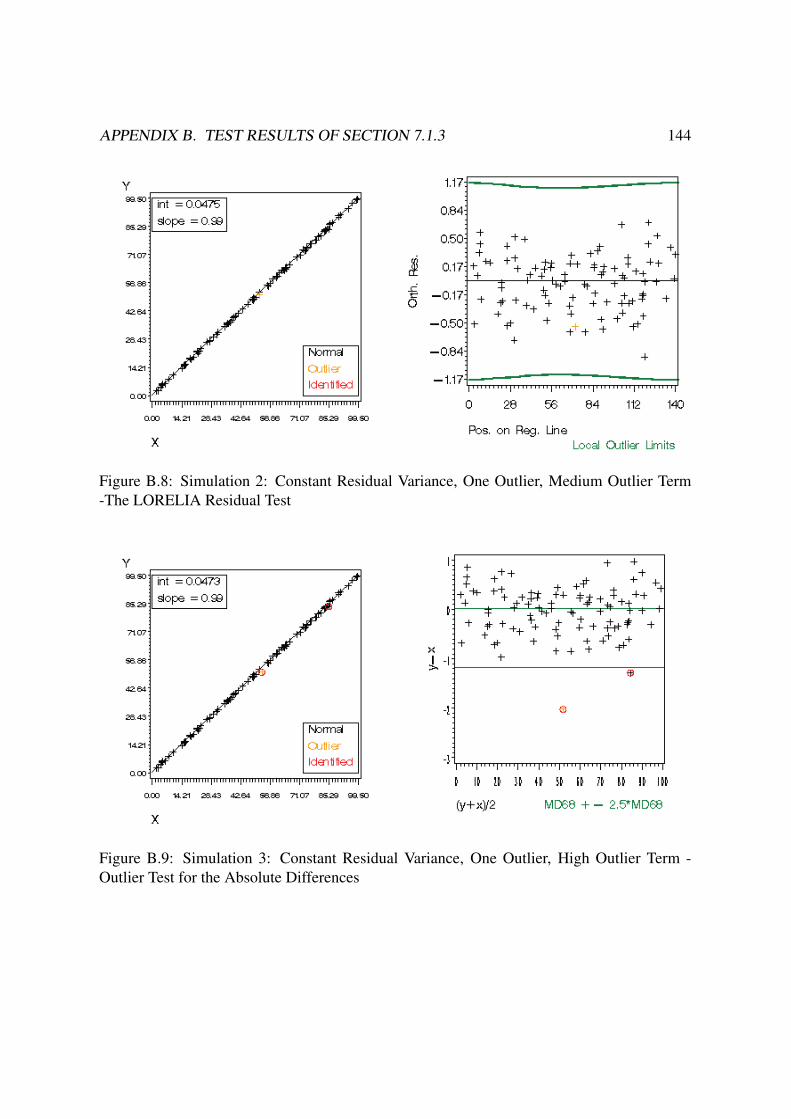
APPENDIX B. TEST RESULTS OF SECTION 7.1.3 144
Figure B.8: Simulation 2: Constant Residual Variance, One Outlier, Medium Outlier Term
-The LORELIA Residual Test
Figure B.9: Simulation 3: Constant Residual Variance, One Outlier, High Outlier Term -
Outlier Test for the Absolute Differences

APPENDIX B. TEST RESULTS OF SECTION 7.1.3 145
Figure B.10: Simulation 3: Constant Residual Variance, One Outlier, High Outlier Term -
Outlier Test for the Normalized Relative Differences
Figure B.11: Simulation 3: Constant Residual Variance, One Outlier, High Outlier Term -
Outlier Test for the Orthogonal Residuals

APPENDIX B. TEST RESULTS OF SECTION 7.1.3 146
Figure B.12: Simulation 3: Constant Residual Variance, One Outlier, High Outlier Term -The
LORELIA Residual Test
Figure B.13: Simulation 4: Constant Residual Variance, Three Outliers, Medium Outlier
Term, Uniformly Distributed Outliers - Outlier Test for the Absolute Differences
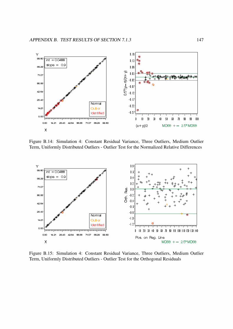
APPENDIX B. TEST RESULTS OF SECTION 7.1.3 147
Figure B.14: Simulation 4: Constant Residual Variance, Three Outliers, Medium Outlier
Term, Uniformly Distributed Outliers - Outlier Test for the Normalized Relative Differences
Figure B.15: Simulation 4: Constant Residual Variance, Three Outliers, Medium Outlier
Term, Uniformly Distributed Outliers - Outlier Test for the Orthogonal Residuals

APPENDIX B. TEST RESULTS OF SECTION 7.1.3 148
Figure B.16: Simulation 4: Constant Residual Variance, Three Outliers, Medium Outlier
Term, Uniformly Distributed Outliers -The LORELIA Residual Test
Figure B.17: Simulation 5: Constant Residual Variance, Three Outliers, Medium Outlier
Term, Clustered Outliers - Outlier Test for the Absolute Differences

APPENDIX B. TEST RESULTS OF SECTION 7.1.3 149
Figure B.18: Simulation 5: Constant Residual Variance, Three Outliers, Medium Outlier
Term, Clustered Outliers - Outlier Test for the Normalized Relative Differences
Figure B.19: Simulation 5: Constant Residual Variance, Three Outliers, Medium Outlier
Term, Clustered Outliers - Outlier Test for the Orthogonal Residuals
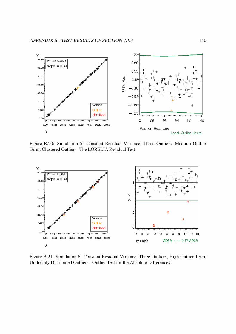
APPENDIX B. TEST RESULTS OF SECTION 7.1.3 150
Figure B.20: Simulation 5: Constant Residual Variance, Three Outliers, Medium Outlier
Term, Clustered Outliers -The LORELIA Residual Test
Figure B.21: Simulation 6: Constant Residual Variance, Three Outliers, High Outlier Term,
Uniformly Distributed Outliers - Outlier Test for the Absolute Differences

APPENDIX B. TEST RESULTS OF SECTION 7.1.3 151
Figure B.22: Simulation 6: Constant Residual Variance, Three Outliers, High Outlier Term,
Uniformly Distributed Outliers - Outlier Test for the Normalized Relative Differences
Figure B.23: Simulation 6: Constant Residual Variance, Three Outliers, High Outlier Term,
Uniformly Distributed Outliers - Outlier Test for the Orthogonal Residuals
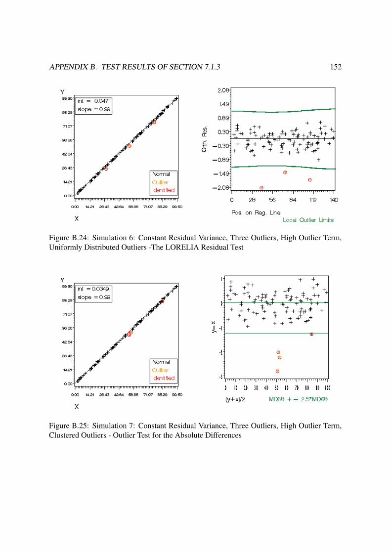
APPENDIX B. TEST RESULTS OF SECTION 7.1.3 152
Figure B.24: Simulation 6: Constant Residual Variance, Three Outliers, High Outlier Term,
Uniformly Distributed Outliers -The LORELIA Residual Test
Figure B.25: Simulation 7: Constant Residual Variance, Three Outliers, High Outlier Term,
Clustered Outliers - Outlier Test for the Absolute Differences

APPENDIX B. TEST RESULTS OF SECTION 7.1.3 153
Figure B.26: Simulation 7: Constant Residual Variance, Three Outliers, High Outlier Term,
Clustered Outliers - Outlier Test for the Normalized Relative Differences
Figure B.27: Simulation 7: Constant Residual Variance, Three Outliers, High Outlier Term,
Clustered Outliers - Outlier Test for the Orthogonal Residuals

APPENDIX B. TEST RESULTS OF SECTION 7.1.3 154
Figure B.28: Simulation 7: Constant Residual Variance, Three Outliers, High Outlier Term,
Clustered Outliers -The LORELIA Residual Test
B.2 Constant Coefficient of Variance
Figure B.29: Simulation 8: Constant Coefficient of Variance, No Outliers - Outlier Test for
the Absolute Differences

APPENDIX B. TEST RESULTS OF SECTION 7.1.3 155
Figure B.30: Simulation 8: Constant Coefficient of Variance, No Outliers - Outlier Test for
the Normalized Relative Differences
Figure B.31: Simulation 8: Constant Coefficient of Variance, No Outliers - Outlier Test for
the Orthogonal Residuals

APPENDIX B. TEST RESULTS OF SECTION 7.1.3 156
Figure B.32: Simulation 8: Constant Coefficient of Variance, No Outliers -The LORELIA
Residual Test
Figure B.33: Simulation 9: Constant Coefficient of Variance, One Outlier, Medium Outlier
Term - Outlier Test for the Absolute Differences

APPENDIX B. TEST RESULTS OF SECTION 7.1.3 157
Figure B.34: Simulation 9: Constant Coefficient of Variance, One Outlier, Medium Outlier
Term - Outlier Test for the Normalized Relative Differences
Figure B.35: Simulation 9: Constant Coefficient of Variance, One Outlier, Medium Outlier
Term - Outlier Test for the Orthogonal Residuals

APPENDIX B. TEST RESULTS OF SECTION 7.1.3 158
Figure B.36: Simulation 9: Constant Coefficient of Variance, One Outlier, Medium Outlier
Term -The LORELIA Residual Test
Figure B.37: Simulation 10: Constant Coefficient of Variance, One Outlier, High Outlier Term
- Outlier Test for the Absolute Differences
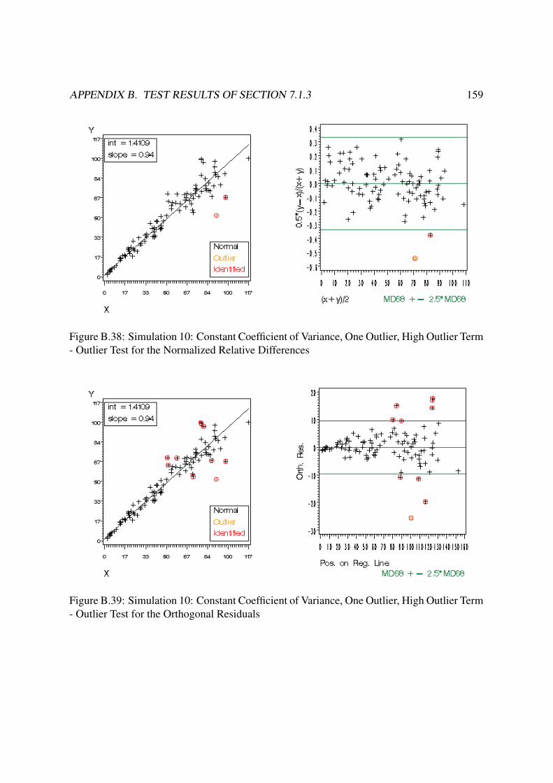
APPENDIX B. TEST RESULTS OF SECTION 7.1.3 159
Figure B.38: Simulation 10: Constant Coefficient of Variance, One Outlier, High Outlier Term
- Outlier Test for the Normalized Relative Differences
Figure B.39: Simulation 10: Constant Coefficient of Variance, One Outlier, High Outlier Term
- Outlier Test for the Orthogonal Residuals
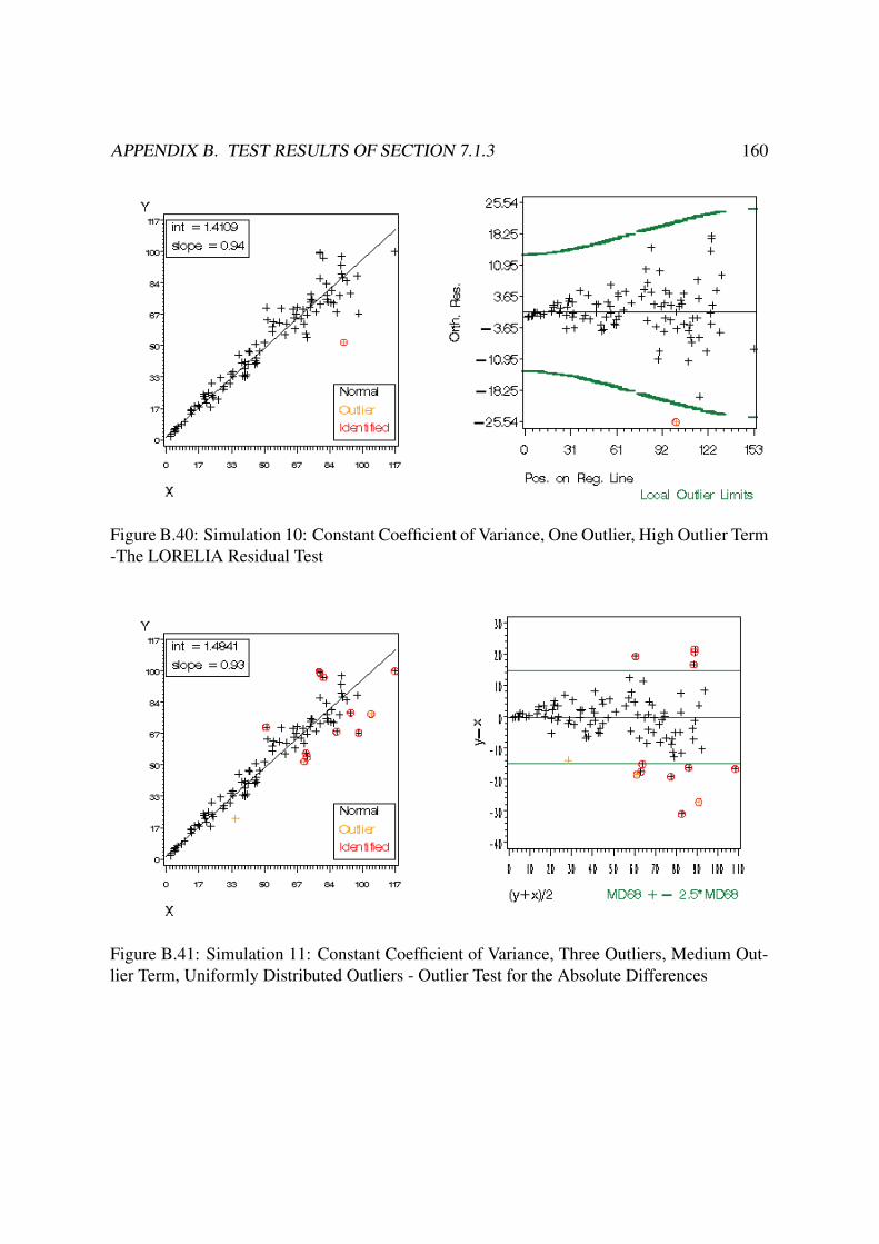
APPENDIX B. TEST RESULTS OF SECTION 7.1.3 160
Figure B.40: Simulation 10: Constant Coefficient of Variance, One Outlier, High Outlier Term
-The LORELIA Residual Test
Figure B.41: Simulation 11: Constant Coefficient of Variance, Three Outliers, Medium Out-
lier Term, Uniformly Distributed Outliers - Outlier Test for the Absolute Differences

APPENDIX B. TEST RESULTS OF SECTION 7.1.3 161
Figure B.42: Simulation 11: Constant Coefficient of Variance, Three Outliers, Medium Out-
lier Term, Uniformly Distributed Outliers - Outlier Test for the Normalized Relative Differ-
ences
Figure B.43: Simulation 11: Constant Coefficient of Variance, Three Outliers, Medium Out-
lier Term, Uniformly Distributed Outliers - Outlier Test for the Orthogonal Residuals

APPENDIX B. TEST RESULTS OF SECTION 7.1.3 162
Figure B.44: Simulation 11: Constant Coefficient of Variance, Three Outliers, Medium Out-
lier Term, Uniformly Distributed Outliers -The LORELIA Residual Test
Figure B.45: Simulation 12: Constant Coefficient of Variance, Three Outliers, Medium Out-
lier Term, Clustered Outliers - Outlier Test for the Absolute Differences
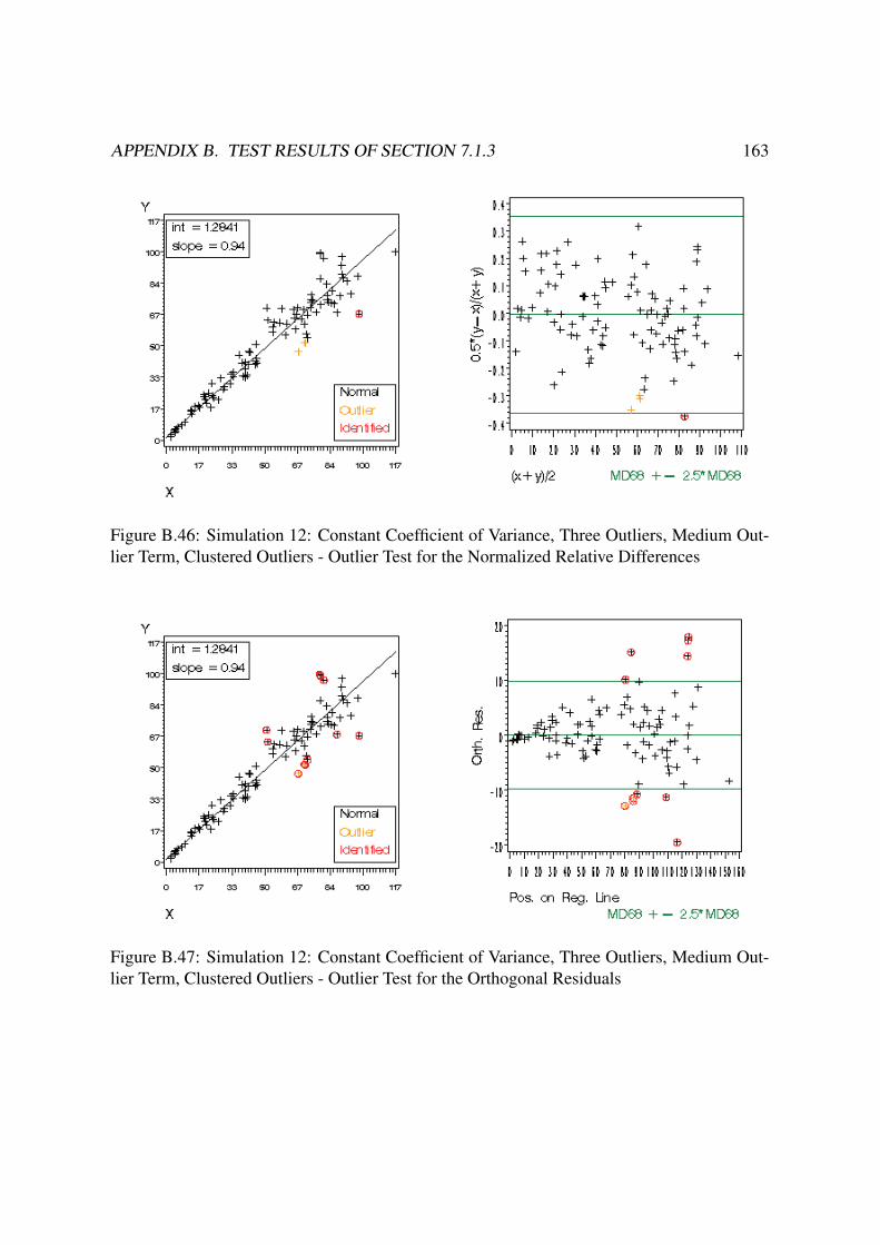
APPENDIX B. TEST RESULTS OF SECTION 7.1.3 163
Figure B.46: Simulation 12: Constant Coefficient of Variance, Three Outliers, Medium Out-
lier Term, Clustered Outliers - Outlier Test for the Normalized Relative Differences
Figure B.47: Simulation 12: Constant Coefficient of Variance, Three Outliers, Medium Out-
lier Term, Clustered Outliers - Outlier Test for the Orthogonal Residuals

APPENDIX B. TEST RESULTS OF SECTION 7.1.3 164
Figure B.48: Simulation 12: Constant Coefficient of Variance, Three Outliers, Medium Out-
lier Term, Clustered Outliers -The LORELIA Residual Test
Figure B.49: Simulation 13: Constant Coefficient of Variance, Three Outliers, High Outlier
Term, Uniformly Distributed Outliers - Outlier Test for the Absolute Differences

APPENDIX B. TEST RESULTS OF SECTION 7.1.3 165
Figure B.50: Simulation 13: Constant Coefficient of Variance, Three Outliers, High Outlier
Term, Uniformly Distributed Outliers - Outlier Test for the Normalized Relative Differences
Figure B.51: Simulation 13: Constant Coefficient of Variance, Three Outliers, High Outlier
Term, Uniformly Distributed Outliers - Outlier Test for the Orthogonal Residuals

APPENDIX B. TEST RESULTS OF SECTION 7.1.3 166
Figure B.52: Simulation 13: Constant Coefficient of Variance, Three Outliers, High Outlier
Term, Uniformly Distributed Outliers -The LORELIA Residual Test
Figure B.53: Simulation 14: Constant Coefficient of Variance, Three Outliers, High Outlier
Term, Clustered Outliers - Outlier Test for the Absolute Differences

APPENDIX B. TEST RESULTS OF SECTION 7.1.3 167
Figure B.54: Simulation 14: Constant Coefficient of Variance, Three Outliers, High Outlier
Term, Clustered Outliers - Outlier Test for the Normalized Relative Differences
Figure B.55: Simulation 14: Constant Coefficient of Variance, Three Outliers, High Outlier
Term, Clustered Outliers - Outlier Test for the Orthogonal Residuals

APPENDIX B. TEST RESULTS OF SECTION 7.1.3 168
Figure B.56: Simulation 14: Constant Coefficient of Variance, Three Outliers, High Outlier
Term, Clustered Outliers -The LORELIA Residual Test
B.3 Non Constant Coefficient of Variance
Figure B.57: Simulation 15: Non Constant Coefficient of Residual Variance, No Outliers -
Outlier Test for the Absolute Differences
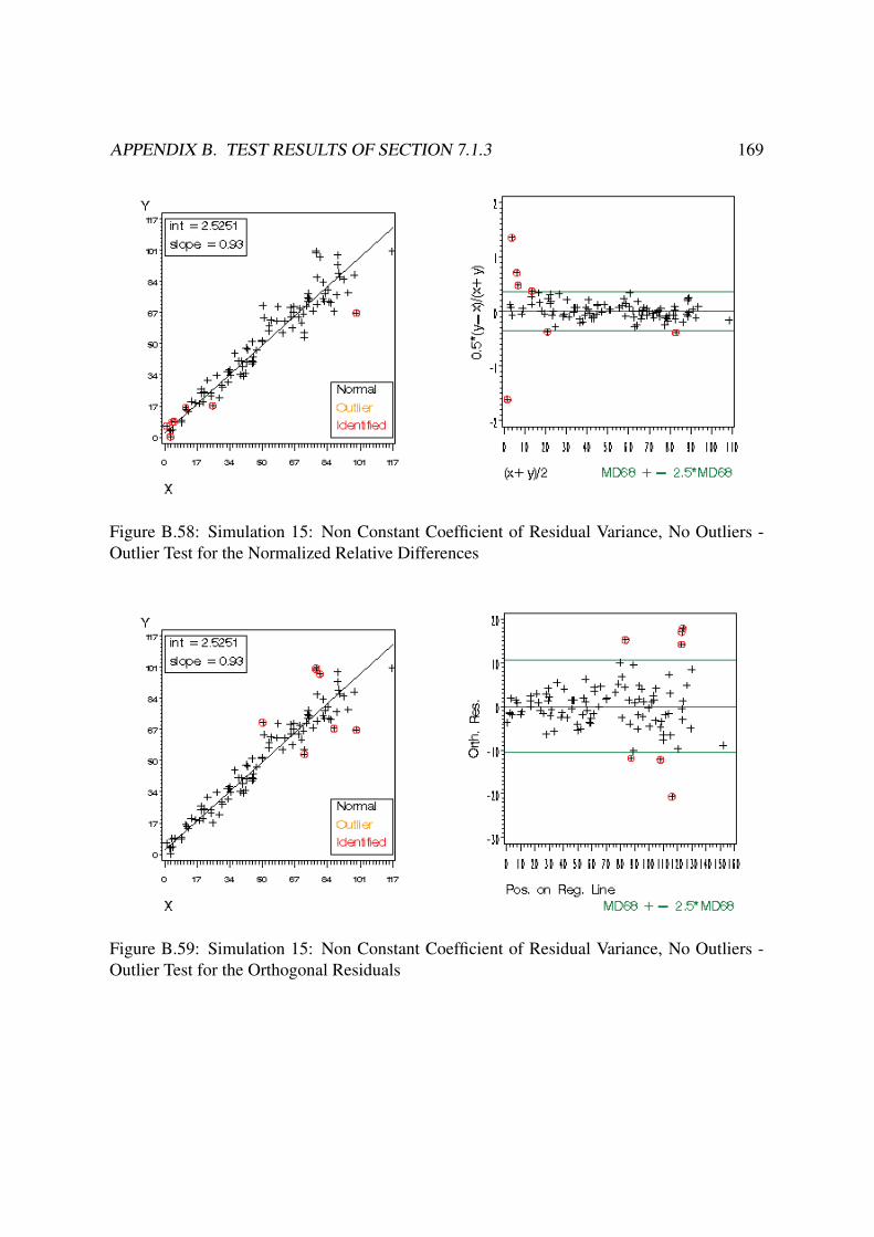
APPENDIX B. TEST RESULTS OF SECTION 7.1.3 169
Figure B.58: Simulation 15: Non Constant Coefficient of Residual Variance, No Outliers -
Outlier Test for the Normalized Relative Differences
Figure B.59: Simulation 15: Non Constant Coefficient of Residual Variance, No Outliers -
Outlier Test for the Orthogonal Residuals

APPENDIX B. TEST RESULTS OF SECTION 7.1.3 170
Figure B.60: Simulation 15: Non Constant Coefficient of Residual Variance, No Outliers -The
LORELIA Residual Test
Figure B.61: Simulation 16: Non Constant Coefficient of Residual Variance, One Outlier,
Medium Outlier Term - Outlier Test for the Absolute Differences

APPENDIX B. TEST RESULTS OF SECTION 7.1.3 171
Figure B.62: Simulation 16: Non Constant Coefficient of Residual Variance, One Outlier,
Medium Outlier Term - Outlier Test for the Normalized Relative Differences
Figure B.63: Simulation 16: Non Constant Coefficient of Residual Variance, One Outlier,
Medium Outlier Term - Outlier Test for the Orthogonal Residuals

APPENDIX B. TEST RESULTS OF SECTION 7.1.3 172
Figure B.64: Simulation 16: Non Constant Coefficient of Residual Variance, One Outlier,
Medium Outlier Term -The LORELIA Residual Test
Figure B.65: Simulation 17: Non Constant Coefficient of Residual Variance, One Outlier,
High Outlier Term - Outlier Test for the Absolute Differences
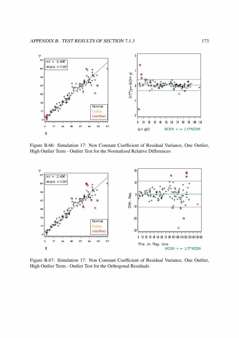
APPENDIX B. TEST RESULTS OF SECTION 7.1.3 173
Figure B.66: Simulation 17: Non Constant Coefficient of Residual Variance, One Outlier,
High Outlier Term - Outlier Test for the Normalized Relative Differences
Figure B.67: Simulation 17: Non Constant Coefficient of Residual Variance, One Outlier,
High Outlier Term - Outlier Test for the Orthogonal Residuals

APPENDIX B. TEST RESULTS OF SECTION 7.1.3 174
Figure B.68: Simulation 17: Non Constant Coefficient of Residual Variance, One Outlier,
High Outlier Term -The LORELIA Residual Test
Figure B.69: Simulation 18: Non Constant Coefficient of Residual Variance, Three Outliers,
Medium Outlier Term, Uniformly Distributed Outliers - Outlier Test for the Absolute Differ-
ences

APPENDIX B. TEST RESULTS OF SECTION 7.1.3 175
Figure B.70: Simulation 18: Non Constant Coefficient of Residual Variance, Three Outliers,
Medium Outlier Term, Uniformly Distributed Outliers - Outlier Test for the Normalized Rel-
ative Differences
Figure B.71: Simulation 18: Non Constant Coefficient of Residual Variance, Three Outliers,
Medium Outlier Term, Uniformly Distributed Outliers - Outlier Test for the Orthogonal Resid-
uals

APPENDIX B. TEST RESULTS OF SECTION 7.1.3 176
Figure B.72: Simulation 18: Non Constant Coefficient of Residual Variance, Three Outliers,
Medium Outlier Term, Uniformly Distributed Outliers -The LORELIA Residual Test
Figure B.73: Simulation 19: Non Constant Coefficient of Residual Variance, Three Outliers,
Medium Outlier Term, Clustered Outliers - Outlier Test for the Absolute Differences

APPENDIX B. TEST RESULTS OF SECTION 7.1.3 177
Figure B.74: Simulation 19: Non Constant Coefficient of Residual Variance, Three Outliers,
Medium Outlier Term, Clustered Outliers - Outlier Test for the Normalized Relative Differ-
ences
Figure B.75: Simulation 19: Non Constant Coefficient of Residual Variance, Three Outliers,
Medium Outlier Term, Clustered Outliers - Outlier Test for the Orthogonal Residuals
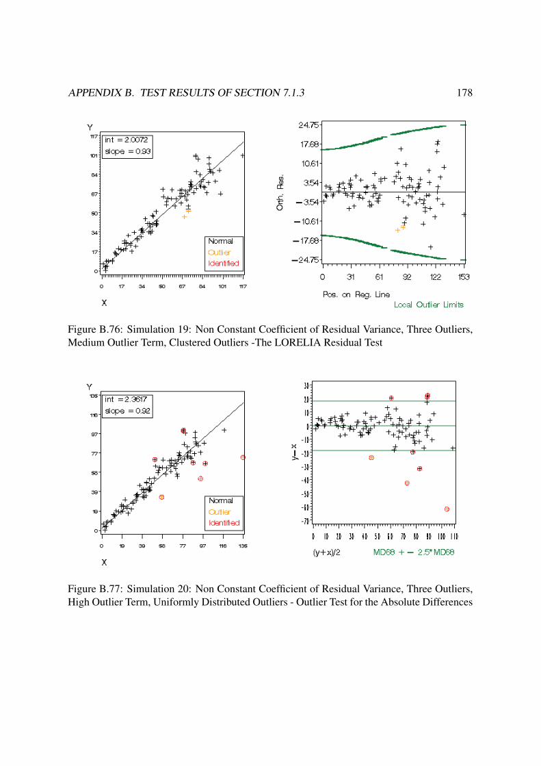
APPENDIX B. TEST RESULTS OF SECTION 7.1.3 178
Figure B.76: Simulation 19: Non Constant Coefficient of Residual Variance, Three Outliers,
Medium Outlier Term, Clustered Outliers -The LORELIA Residual Test
Figure B.77: Simulation 20: Non Constant Coefficient of Residual Variance, Three Outliers,
High Outlier Term, Uniformly Distributed Outliers - Outlier Test for the Absolute Differences

APPENDIX B. TEST RESULTS OF SECTION 7.1.3 179
Figure B.78: Simulation 20: Non Constant Coefficient of Residual Variance, Three Outliers,
High Outlier Term, Uniformly Distributed Outliers - Outlier Test for the Normalized Relative
Differences
Figure B.79: Simulation 20: Non Constant Coefficient of Residual Variance, Three Outliers,
High Outlier Term, Uniformly Distributed Outliers - Outlier Test for the Orthogonal Residuals

APPENDIX B. TEST RESULTS OF SECTION 7.1.3 180
Figure B.80: Simulation 20: Non Constant Coefficient of Residual Variance, Three Outliers,
High Outlier Term, Uniformly Distributed Outliers -The LORELIA Residual Test
Figure B.81: Simulation 21: Non Constant Coefficient of Residual Variance, Three Outliers,
High Outlier Term, Clustered Outliers - Outlier Test for the Absolute Differences

APPENDIX B. TEST RESULTS OF SECTION 7.1.3 181
Figure B.82: Simulation 21: Non Constant Coefficient of Residual Variance, Three Outliers,
High Outlier Term, Clustered Outliers - Outlier Test for the Normalized Relative Differences
Figure B.83: Simulation 21: Non Constant Coefficient of Residual Variance, Three Outliers,
High Outlier Term, Clustered Outliers - Outlier Test for the Orthogonal Residuals

APPENDIX B. TEST RESULTS OF SECTION 7.1.3 182
Figure B.84: Simulation 21: Non Constant Coefficient of Residual Variance, Three Outliers,
High Outlier Term, Clustered Outliers -The LORELIA Residual Test

Symbols
N Natural Numbers
R Real Numbers
R+0 Positive Real Numbers Including 0
U(a, b) Continuous Uniform Distribution on [a, b] ⊂ R
N(μ, σ2) Normal Distribution with Expected Value μ and Variance σ2
logN(μ, σ2) Log Normal Distribution with Parameters μ and σ2
χ2DF χ2 Distribution with DF Degrees of Freedom
Φ() Distribution Function of the Standard Normal Distribution
z(1−α) (1− α) Quantile of the Standard Normal Distribution
tDF,(1−α) (1 − α) Quantile of the Students t Distribution with DF Degrees of
Freedom
X1, ..., Xniid∼ X X1, ..., Xn are independent and identically distributed as X
x1, ..., xn Realizations of the Random Variables X1, ..., Xn
x(1), ..., x(n) Ordered Sequence of x1, ..., xn
E(X) Expected Value of the Random Variable XV ar(X) Variance of the Random Variable Xx Mean Value of x1, ..., xn given by 1
n
∑ni=1 xi
S2xx Empirical Variance of X given by 1
n−1
∑ni=1(xi − x)2
S2xy Empirical Covariance of X and Y given by 1
n−1
∑ni=1(xi − x)(yi − y)
med(x) Median of x1, ..., xn
mad68(x) 68% Median Absolute Deviation
min{1≤i≤n} {xi} Minimum of x1, ..., xn
max{1≤i≤n} {xi} Maximum of x1, ..., xn
inf{1≤i≤n} {xi} Infimum of x1, ..., xn
sup{1≤i≤n} {xi} Supremum of x1, ..., xn
sign() Signum Function
mod() Modulus Function∂f∂t
Partial Derivative of the Function f to t
183

SYMBOLS 184
H0 Null Hypothesis of a Statistical Test
H1 Alternative Hypothesis of a Statistical Test
α Level of Significance
αloc Local Level of Significance for a Multiple Test Situation
αglob Global Level of Significance for a Multiple Test Situation
Pint Population of Interest
Pcont Contaminating Population
Mx, My Methods which are to be compared
X, Y Random Variables for the True Measurement Values of Methods Mx
and My
Ex, Ey Random Variables for the Measurement Errors in Methods Mx and My
c1, ..., cn True Concentrations for Measurement Values (x1, y1), ..., (xn, yn)R1, ..., Rn Random Variables for the Orthogonal Residuals
outx, outy Outlier Term for Methods Mx and My
Dabsi Random Variable for the Absolute Difference between x and y
Dreli Random Variable for the Relative Difference between x and y
Dnormreli Random Variable for the Normalized Relative Difference between x and
y
αPCA, βPCA Parameter Estimators for Principal Component Analysis
αSPCA, βSPCA Parameter Estimators for Standardized Principal Component Analysis
αPB, βPB Parameter Estimators for Passing-Bablok Regression
R2 Squared Correlation Coefficient for Linear Regression
Cα (1− α)% Approximative Confidence Intervall
(xpi , y
pi ) Orthogonal Projection of the Measurement Tuple (xi, yi) to the Regres-
sion Line
wShep Shepard’s Weights (Inverse Distance Weights)
wKon Weights proposed by [Konnert, 2005]
wik LORELIA Weights
δik Squared Absolute Distance between (xpi , y
pi ) and (xp
k, ypk)
Δik LORELIA Distance Weight, Transformation of δik
γk,n Reliability Measure
Γk,n LORELIA Reliability Weight, Transformation of γk,n

List of Figures
2.1 Outliers in Different Data Situations - Bar Diagram . . . . . . . . . . . . . . 6
2.2 Outliers in Different Data Situations - Linear Model . . . . . . . . . . . . . . 7
2.3 Outliers in Different Data Situations - Normal Distribution . . . . . . . . . . 7
2.4 Mixed Distribution: 0.9 ·N(3, 1) + 0.1 · logN(7, 1) . . . . . . . . . . . . . . 9
2.5 Mixed Distribution: 0.9 ·N(5, 1) + 0.1 · logN(5, 2) . . . . . . . . . . . . . . 10
2.6 Population Affiliations . . . . . . . . . . . . . . . . . . . . . . . . . . . . . 11
2.7 Extreme Observation for the U-Distribution . . . . . . . . . . . . . . . . . . 12
2.8 Error in the Model Assumption . . . . . . . . . . . . . . . . . . . . . . . . . 13
2.9 Corrected Model Assumption . . . . . . . . . . . . . . . . . . . . . . . . . . 13
2.10 Outlier Candidate from a Two-Dimensional Linear Regression Model . . . . 14
2.11 Outlier Candidates in Location and in Variance . . . . . . . . . . . . . . . . 15
2.12 Ambiguity of Extreme Values . . . . . . . . . . . . . . . . . . . . . . . . . 15
2.13 Linear Fits for Excluded Upper or Lower Extreme Value . . . . . . . . . . . 16
2.14 Linear Fits with both Extreme Values Excluded . . . . . . . . . . . . . . . . 17
2.15 Classification of Outlier Candidates . . . . . . . . . . . . . . . . . . . . . . 19
3.1 The Masking Effect . . . . . . . . . . . . . . . . . . . . . . . . . . . . . . . 26
3.2 The Swamping Effect . . . . . . . . . . . . . . . . . . . . . . . . . . . . . . 26
3.3 Linear Regression with the First Leverage Point Included . . . . . . . . . . . 28
3.4 Linear Regression with the Second Leverage Point Included . . . . . . . . . 28
3.5 Linear Regression without the Leverage Points . . . . . . . . . . . . . . . . 29
4.1 Method Comparison based on the Absolute Differences . . . . . . . . . . . . 32
4.2 Proportional Bias Between Methods . . . . . . . . . . . . . . . . . . . . . . 33
4.3 Method Comparison based on the Normalized Relative Differences . . . . . . 34
4.4 Method Comparison based on the Relative Differences . . . . . . . . . . . . 36
4.5 The Concept of Deming Regression . . . . . . . . . . . . . . . . . . . . . . 38
4.6 Residuals for PCA and SPCA . . . . . . . . . . . . . . . . . . . . . . . . . . 40
185
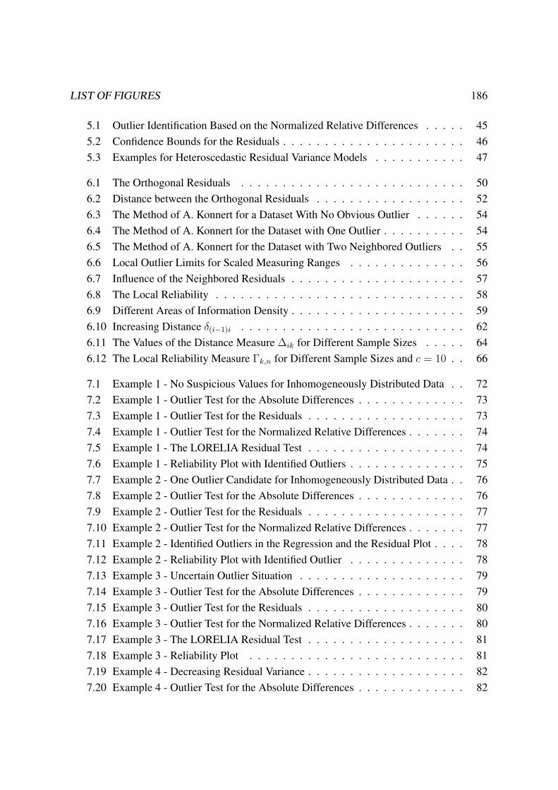
LIST OF FIGURES 186
5.1 Outlier Identification Based on the Normalized Relative Differences . . . . . 45
5.2 Confidence Bounds for the Residuals . . . . . . . . . . . . . . . . . . . . . . 46
5.3 Examples for Heteroscedastic Residual Variance Models . . . . . . . . . . . 47
6.1 The Orthogonal Residuals . . . . . . . . . . . . . . . . . . . . . . . . . . . 50
6.2 Distance between the Orthogonal Residuals . . . . . . . . . . . . . . . . . . 52
6.3 The Method of A. Konnert for a Dataset With No Obvious Outlier . . . . . . 54
6.4 The Method of A. Konnert for the Dataset with One Outlier . . . . . . . . . . 54
6.5 The Method of A. Konnert for the Dataset with Two Neighbored Outliers . . 55
6.6 Local Outlier Limits for Scaled Measuring Ranges . . . . . . . . . . . . . . 56
6.7 Influence of the Neighbored Residuals . . . . . . . . . . . . . . . . . . . . . 57
6.8 The Local Reliability . . . . . . . . . . . . . . . . . . . . . . . . . . . . . . 58
6.9 Different Areas of Information Density . . . . . . . . . . . . . . . . . . . . . 59
6.10 Increasing Distance δ(i−1)i . . . . . . . . . . . . . . . . . . . . . . . . . . . 62
6.11 The Values of the Distance Measure Δik for Different Sample Sizes . . . . . 64
6.12 The Local Reliability Measure Γk,n for Different Sample Sizes and c = 10 . . 66
7.1 Example 1 - No Suspicious Values for Inhomogeneously Distributed Data . . 72
7.2 Example 1 - Outlier Test for the Absolute Differences . . . . . . . . . . . . . 73
7.3 Example 1 - Outlier Test for the Residuals . . . . . . . . . . . . . . . . . . . 73
7.4 Example 1 - Outlier Test for the Normalized Relative Differences . . . . . . . 74
7.5 Example 1 - The LORELIA Residual Test . . . . . . . . . . . . . . . . . . . 74
7.6 Example 1 - Reliability Plot with Identified Outliers . . . . . . . . . . . . . . 75
7.7 Example 2 - One Outlier Candidate for Inhomogeneously Distributed Data . . 76
7.8 Example 2 - Outlier Test for the Absolute Differences . . . . . . . . . . . . . 76
7.9 Example 2 - Outlier Test for the Residuals . . . . . . . . . . . . . . . . . . . 77
7.10 Example 2 - Outlier Test for the Normalized Relative Differences . . . . . . . 77
7.11 Example 2 - Identified Outliers in the Regression and the Residual Plot . . . . 78
7.12 Example 2 - Reliability Plot with Identified Outlier . . . . . . . . . . . . . . 78
7.13 Example 3 - Uncertain Outlier Situation . . . . . . . . . . . . . . . . . . . . 79
7.14 Example 3 - Outlier Test for the Absolute Differences . . . . . . . . . . . . . 79
7.15 Example 3 - Outlier Test for the Residuals . . . . . . . . . . . . . . . . . . . 80
7.16 Example 3 - Outlier Test for the Normalized Relative Differences . . . . . . . 80
7.17 Example 3 - The LORELIA Residual Test . . . . . . . . . . . . . . . . . . . 81
7.18 Example 3 - Reliability Plot . . . . . . . . . . . . . . . . . . . . . . . . . . 81
7.19 Example 4 - Decreasing Residual Variance . . . . . . . . . . . . . . . . . . . 82
7.20 Example 4 - Outlier Test for the Absolute Differences . . . . . . . . . . . . . 82

LIST OF FIGURES 187
7.21 Example 4 - Outlier Test for the Residuals . . . . . . . . . . . . . . . . . . . 83
7.22 Example 4 - Outlier Test for the Normalized Relative Differences . . . . . . . 83
7.23 Example 4 - The LORELIA Residual Test . . . . . . . . . . . . . . . . . . . 84
7.24 Example 4 - Reliability Plot with Identified Outliers . . . . . . . . . . . . . . 84
7.25 Example 5 - Very Inhomogeneous Data Dispersion . . . . . . . . . . . . . . 85
7.26 Example 5 - Outlier Test for the Absolute Differences . . . . . . . . . . . . . 85
7.27 Example 5 - Outlier Test for the Residuals . . . . . . . . . . . . . . . . . . . 86
7.28 Example 5 - Outlier Test for the Normalized Relative Differences . . . . . . . 86
7.29 Example 5 - The LORELIA Residual Test . . . . . . . . . . . . . . . . . . . 87
7.30 Example 5 - Reliability Plot with Identified Outliers . . . . . . . . . . . . . . 87
7.31 Exemplary Dataset from the Model Class M . . . . . . . . . . . . . . . . . . 94
7.32 Evaluation of the Exemplary Dataset with the Global Outlier Tests Based on
the Absolute Differences, on the Orthogonal Residuals and on the Normalized
Relative Differences . . . . . . . . . . . . . . . . . . . . . . . . . . . . . . . 95
7.33 Evaluation of the Exemplary Dataset with the LORELIA Residual Test . . . . 95
7.34 Percentages of True Positive Test Results, Constant Residual Variance . . . . 101
7.35 Percentages of False Positive Test Results, Constant Residual Variance . . . . 102
7.36 Percentages of True Positive Test Results for a Constant Coefficient of Variance103
7.37 Percentages of False Positive Test Results for a Constant Coefficient of Variance104
7.38 Percentages of True Positive Test Results, Non Constant Coefficient of Variance106
7.39 Means of True Positive and False Positive Test Results - Homogeneous Data
Distribution, Non Constant Coefficient of Variance . . . . . . . . . . . . . . 106
7.40 Homogeneous Data Distribution, Constant Coefficient of Variance, Three Out-
liers, Medium Outlier Term, Uniformly Distributed Outliers . . . . . . . . . 108
7.41 Homogeneous Data Distribution, Constant Residual Variance, Three Outliers,
Medium Outlier Term, Clustered Outliers . . . . . . . . . . . . . . . . . . . 109
7.42 The Outlier Residual . . . . . . . . . . . . . . . . . . . . . . . . . . . . . . 114
7.43 Relation between Outlier Position and Percentages of True Positive Test Re-
sults - Homogeneous Data Distribution, Constant Residual Variance, Medium
Outlier Term . . . . . . . . . . . . . . . . . . . . . . . . . . . . . . . . . . . 115
7.44 Polynomial Fit for Percentages of True Positive Test Results - Homogeneous
Data Distribution, Constant Residual Variance, Medium Outlier Term . . . . 116
7.45 Relation between Outlier Position and Percentages of True Positive Test Re-
sults - Homogeneous Data Distribution, Constant Residual Variance, High
Outlier Term . . . . . . . . . . . . . . . . . . . . . . . . . . . . . . . . . . . 117
7.46 Relation between Outlier Position and Percentages of True Positive Test Re-
sults - Homogeneous Data Distribution, Constant Coefficient of Variance,
Medium Outlier Term . . . . . . . . . . . . . . . . . . . . . . . . . . . . . . 119

LIST OF FIGURES 188
7.47 Relation between Outlier Position and Percentages of True Positive Test Re-
sults - Homogeneous Data Distribution, Constant Coefficient of Variance,
High Outlier Term . . . . . . . . . . . . . . . . . . . . . . . . . . . . . . . . 119
7.48 Relation between Outlier Position and Percentages of True Positive Test Re-
sults - Inhomogeneous Data Distribution, Constant Residual Variance, Medium
Outlier Term . . . . . . . . . . . . . . . . . . . . . . . . . . . . . . . . . . . 121
7.49 Relation between Outlier Location and Percentages of True Positive Test Re-
sults - Inhomogeneous Data Distribution, Constant Residual Variance, Medium
Outlier Term . . . . . . . . . . . . . . . . . . . . . . . . . . . . . . . . . . . 122
7.50 Relation between Outlier Position and Percentages of True Positive Test Re-
sults - Inhomogeneous Data Distribution, Constant Residual Variance, High
Outlier Term . . . . . . . . . . . . . . . . . . . . . . . . . . . . . . . . . . . 122
7.51 Relation between Outlier Location and Percentages of True Positive Test Re-
sults - Inhomogeneous Data Distribution, Constant Residual Variance, High
Outlier Term . . . . . . . . . . . . . . . . . . . . . . . . . . . . . . . . . . . 123
7.52 Relation between Outlier Position and Percentages of True Positive Test Re-
sults - Inhomogeneous Data Distribution, Constant Coefficient of Variance,
Medium Outlier Term . . . . . . . . . . . . . . . . . . . . . . . . . . . . . . 124
7.53 Relation between Outlier Location and Percentages of True Positive Test Re-
sults - Histogram, Inhomogeneous Data Distribution, Constant Coefficient of
Variance, Medium Outlier Term . . . . . . . . . . . . . . . . . . . . . . . . 125
7.54 Relation between Outlier Position and Percentages of True Positive Test Re-
sults - Inhomogeneous Data Distribution, Constant Coefficient of Variance,
High Outlier Term . . . . . . . . . . . . . . . . . . . . . . . . . . . . . . . . 125
7.55 Relation between Outlier Location and Percentages of True Positive Test Re-
sults - Histogram, Inhomogeneous Data Distribution, Constant Coefficient of
Variance, High Outlier Term . . . . . . . . . . . . . . . . . . . . . . . . . . 126
7.56 Exemplary Dataset - Bad Performance of the LORELIA Residual Test . . . . 127
7.57 Exemplary Dataset - Reliability Plot . . . . . . . . . . . . . . . . . . . . . . 127
7.58 Exemplary Dataset, Low Part - Improved Performance . . . . . . . . . . . . 128
7.59 Exemplary Dataset, Low Part - Reliability Plot . . . . . . . . . . . . . . . . . 128
7.60 Exemplary Dataset, Upper Part - Improved Performance . . . . . . . . . . . 129
7.61 Exemplary Dataset, High Part - Reliability Plot . . . . . . . . . . . . . . . . 129
A.1 Documented SAS® Program Files with Brief Descriptions . . . . . . . . . . 139
B.1 Simulation 1: Constant Residual Variance, No Outliers - Outlier Test for the
Absolute Differences . . . . . . . . . . . . . . . . . . . . . . . . . . . . . . 140
B.2 Simulation 1: Constant Residual Variance, No Outliers - Outlier Test for the
Normalized Relative Differences . . . . . . . . . . . . . . . . . . . . . . . . 141

LIST OF FIGURES 189
B.3 Simulation 1: Constant Residual Variance, No Outliers - Outlier Test for the
Orthogonal Residuals . . . . . . . . . . . . . . . . . . . . . . . . . . . . . . 141
B.4 Simulation 1: Constant Residual Variance, No Outliers -The LORELIA Resid-
ual Test . . . . . . . . . . . . . . . . . . . . . . . . . . . . . . . . . . . . . 142
B.5 Simulation 2: Constant Residual Variance, One Outlier, Medium Outlier Term
- Outlier Test for the Absolute Differences . . . . . . . . . . . . . . . . . . . 142
B.6 Simulation 2: Constant Residual Variance, One Outlier, Medium Outlier Term
- Outlier Test for the Normalized Relative Differences . . . . . . . . . . . . . 143
B.7 Simulation 2: Constant Residual Variance, One Outlier, Medium Outlier Term
- Outlier Test for the Orthogonal Residuals . . . . . . . . . . . . . . . . . . . 143
B.8 Simulation 2: Constant Residual Variance, One Outlier, Medium Outlier Term
-The LORELIA Residual Test . . . . . . . . . . . . . . . . . . . . . . . . . 144
B.9 Simulation 3: Constant Residual Variance, One Outlier, High Outlier Term -
Outlier Test for the Absolute Differences . . . . . . . . . . . . . . . . . . . . 144
B.10 Simulation 3: Constant Residual Variance, One Outlier, High Outlier Term -
Outlier Test for the Normalized Relative Differences . . . . . . . . . . . . . 145
B.11 Simulation 3: Constant Residual Variance, One Outlier, High Outlier Term -
Outlier Test for the Orthogonal Residuals . . . . . . . . . . . . . . . . . . . 145
B.12 Simulation 3: Constant Residual Variance, One Outlier, High Outlier Term
-The LORELIA Residual Test . . . . . . . . . . . . . . . . . . . . . . . . . 146
B.13 Simulation 4: Constant Residual Variance, Three Outliers, Medium Outlier
Term, Uniformly Distributed Outliers - Outlier Test for the Absolute Differences146
B.14 Simulation 4: Constant Residual Variance, Three Outliers, Medium Outlier
Term, Uniformly Distributed Outliers - Outlier Test for the Normalized Rela-
tive Differences . . . . . . . . . . . . . . . . . . . . . . . . . . . . . . . . . 147
B.15 Simulation 4: Constant Residual Variance, Three Outliers, Medium Outlier
Term, Uniformly Distributed Outliers - Outlier Test for the Orthogonal Residuals147
B.16 Simulation 4: Constant Residual Variance, Three Outliers, Medium Outlier
Term, Uniformly Distributed Outliers -The LORELIA Residual Test . . . . . 148
B.17 Simulation 5: Constant Residual Variance, Three Outliers, Medium Outlier
Term, Clustered Outliers - Outlier Test for the Absolute Differences . . . . . 148
B.18 Simulation 5: Constant Residual Variance, Three Outliers, Medium Outlier
Term, Clustered Outliers - Outlier Test for the Normalized Relative Differences 149
B.19 Simulation 5: Constant Residual Variance, Three Outliers, Medium Outlier
Term, Clustered Outliers - Outlier Test for the Orthogonal Residuals . . . . . 149
B.20 Simulation 5: Constant Residual Variance, Three Outliers, Medium Outlier
Term, Clustered Outliers -The LORELIA Residual Test . . . . . . . . . . . . 150
B.21 Simulation 6: Constant Residual Variance, Three Outliers, High Outlier Term,
Uniformly Distributed Outliers - Outlier Test for the Absolute Differences . . 150

LIST OF FIGURES 190
B.22 Simulation 6: Constant Residual Variance, Three Outliers, High Outlier Term,
Uniformly Distributed Outliers - Outlier Test for the Normalized Relative Dif-
ferences . . . . . . . . . . . . . . . . . . . . . . . . . . . . . . . . . . . . . 151
B.23 Simulation 6: Constant Residual Variance, Three Outliers, High Outlier Term,
Uniformly Distributed Outliers - Outlier Test for the Orthogonal Residuals . . 151
B.24 Simulation 6: Constant Residual Variance, Three Outliers, High Outlier Term,
Uniformly Distributed Outliers -The LORELIA Residual Test . . . . . . . . 152
B.25 Simulation 7: Constant Residual Variance, Three Outliers, High Outlier Term,
Clustered Outliers - Outlier Test for the Absolute Differences . . . . . . . . . 152
B.26 Simulation 7: Constant Residual Variance, Three Outliers, High Outlier Term,
Clustered Outliers - Outlier Test for the Normalized Relative Differences . . . 153
B.27 Simulation 7: Constant Residual Variance, Three Outliers, High Outlier Term,
Clustered Outliers - Outlier Test for the Orthogonal Residuals . . . . . . . . 153
B.28 Simulation 7: Constant Residual Variance, Three Outliers, High Outlier Term,
Clustered Outliers -The LORELIA Residual Test . . . . . . . . . . . . . . . 154
B.29 Simulation 8: Constant Coefficient of Variance, No Outliers - Outlier Test for
the Absolute Differences . . . . . . . . . . . . . . . . . . . . . . . . . . . . 154
B.30 Simulation 8: Constant Coefficient of Variance, No Outliers - Outlier Test for
the Normalized Relative Differences . . . . . . . . . . . . . . . . . . . . . . 155
B.31 Simulation 8: Constant Coefficient of Variance, No Outliers - Outlier Test for
the Orthogonal Residuals . . . . . . . . . . . . . . . . . . . . . . . . . . . . 155
B.32 Simulation 8: Constant Coefficient of Variance, No Outliers -The LORELIA
Residual Test . . . . . . . . . . . . . . . . . . . . . . . . . . . . . . . . . . 156
B.33 Simulation 9: Constant Coefficient of Variance, One Outlier, Medium Outlier
Term - Outlier Test for the Absolute Differences . . . . . . . . . . . . . . . . 156
B.34 Simulation 9: Constant Coefficient of Variance, One Outlier, Medium Outlier
Term - Outlier Test for the Normalized Relative Differences . . . . . . . . . 157
B.35 Simulation 9: Constant Coefficient of Variance, One Outlier, Medium Outlier
Term - Outlier Test for the Orthogonal Residuals . . . . . . . . . . . . . . . 157
B.36 Simulation 9: Constant Coefficient of Variance, One Outlier, Medium Outlier
Term -The LORELIA Residual Test . . . . . . . . . . . . . . . . . . . . . . 158
B.37 Simulation 10: Constant Coefficient of Variance, One Outlier, High Outlier
Term - Outlier Test for the Absolute Differences . . . . . . . . . . . . . . . . 158
B.38 Simulation 10: Constant Coefficient of Variance, One Outlier, High Outlier
Term - Outlier Test for the Normalized Relative Differences . . . . . . . . . 159
B.39 Simulation 10: Constant Coefficient of Variance, One Outlier, High Outlier
Term - Outlier Test for the Orthogonal Residuals . . . . . . . . . . . . . . . 159
B.40 Simulation 10: Constant Coefficient of Variance, One Outlier, High Outlier
Term -The LORELIA Residual Test . . . . . . . . . . . . . . . . . . . . . . 160

LIST OF FIGURES 191
B.41 Simulation 11: Constant Coefficient of Variance, Three Outliers, Medium
Outlier Term, Uniformly Distributed Outliers - Outlier Test for the Absolute
Differences . . . . . . . . . . . . . . . . . . . . . . . . . . . . . . . . . . . 160
B.42 Simulation 11: Constant Coefficient of Variance, Three Outliers, Medium
Outlier Term, Uniformly Distributed Outliers - Outlier Test for the Normal-
ized Relative Differences . . . . . . . . . . . . . . . . . . . . . . . . . . . . 161
B.43 Simulation 11: Constant Coefficient of Variance, Three Outliers, Medium
Outlier Term, Uniformly Distributed Outliers - Outlier Test for the Orthogonal
Residuals . . . . . . . . . . . . . . . . . . . . . . . . . . . . . . . . . . . . 161
B.44 Simulation 11: Constant Coefficient of Variance, Three Outliers, Medium
Outlier Term, Uniformly Distributed Outliers -The LORELIA Residual Test . 162
B.45 Simulation 12: Constant Coefficient of Variance, Three Outliers, Medium
Outlier Term, Clustered Outliers - Outlier Test for the Absolute Differences . 162
B.46 Simulation 12: Constant Coefficient of Variance, Three Outliers, Medium
Outlier Term, Clustered Outliers - Outlier Test for the Normalized Relative
Differences . . . . . . . . . . . . . . . . . . . . . . . . . . . . . . . . . . . 163
B.47 Simulation 12: Constant Coefficient of Variance, Three Outliers, Medium
Outlier Term, Clustered Outliers - Outlier Test for the Orthogonal Residuals . 163
B.48 Simulation 12: Constant Coefficient of Variance, Three Outliers, Medium
Outlier Term, Clustered Outliers -The LORELIA Residual Test . . . . . . . . 164
B.49 Simulation 13: Constant Coefficient of Variance, Three Outliers, High Outlier
Term, Uniformly Distributed Outliers - Outlier Test for the Absolute Differences164
B.50 Simulation 13: Constant Coefficient of Variance, Three Outliers, High Out-
lier Term, Uniformly Distributed Outliers - Outlier Test for the Normalized
Relative Differences . . . . . . . . . . . . . . . . . . . . . . . . . . . . . . . 165
B.51 Simulation 13: Constant Coefficient of Variance, Three Outliers, High Outlier
Term, Uniformly Distributed Outliers - Outlier Test for the Orthogonal Residuals165
B.52 Simulation 13: Constant Coefficient of Variance, Three Outliers, High Outlier
Term, Uniformly Distributed Outliers -The LORELIA Residual Test . . . . . 166
B.53 Simulation 14: Constant Coefficient of Variance, Three Outliers, High Outlier
Term, Clustered Outliers - Outlier Test for the Absolute Differences . . . . . 166
B.54 Simulation 14: Constant Coefficient of Variance, Three Outliers, High Outlier
Term, Clustered Outliers - Outlier Test for the Normalized Relative Differences 167
B.55 Simulation 14: Constant Coefficient of Variance, Three Outliers, High Outlier
Term, Clustered Outliers - Outlier Test for the Orthogonal Residuals . . . . . 167
B.56 Simulation 14: Constant Coefficient of Variance, Three Outliers, High Outlier
Term, Clustered Outliers -The LORELIA Residual Test . . . . . . . . . . . . 168
B.57 Simulation 15: Non Constant Coefficient of Residual Variance, No Outliers -
Outlier Test for the Absolute Differences . . . . . . . . . . . . . . . . . . . . 168

LIST OF FIGURES 192
B.58 Simulation 15: Non Constant Coefficient of Residual Variance, No Outliers -
Outlier Test for the Normalized Relative Differences . . . . . . . . . . . . . 169
B.59 Simulation 15: Non Constant Coefficient of Residual Variance, No Outliers -
Outlier Test for the Orthogonal Residuals . . . . . . . . . . . . . . . . . . . 169
B.60 Simulation 15: Non Constant Coefficient of Residual Variance, No Outliers
-The LORELIA Residual Test . . . . . . . . . . . . . . . . . . . . . . . . . 170
B.61 Simulation 16: Non Constant Coefficient of Residual Variance, One Outlier,
Medium Outlier Term - Outlier Test for the Absolute Differences . . . . . . . 170
B.62 Simulation 16: Non Constant Coefficient of Residual Variance, One Outlier,
Medium Outlier Term - Outlier Test for the Normalized Relative Differences . 171
B.63 Simulation 16: Non Constant Coefficient of Residual Variance, One Outlier,
Medium Outlier Term - Outlier Test for the Orthogonal Residuals . . . . . . 171
B.64 Simulation 16: Non Constant Coefficient of Residual Variance, One Outlier,
Medium Outlier Term -The LORELIA Residual Test . . . . . . . . . . . . . 172
B.65 Simulation 17: Non Constant Coefficient of Residual Variance, One Outlier,
High Outlier Term - Outlier Test for the Absolute Differences . . . . . . . . . 172
B.66 Simulation 17: Non Constant Coefficient of Residual Variance, One Outlier,
High Outlier Term - Outlier Test for the Normalized Relative Differences . . 173
B.67 Simulation 17: Non Constant Coefficient of Residual Variance, One Outlier,
High Outlier Term - Outlier Test for the Orthogonal Residuals . . . . . . . . 173
B.68 Simulation 17: Non Constant Coefficient of Residual Variance, One Outlier,
High Outlier Term -The LORELIA Residual Test . . . . . . . . . . . . . . . 174
B.69 Simulation 18: Non Constant Coefficient of Residual Variance, Three Out-
liers, Medium Outlier Term, Uniformly Distributed Outliers - Outlier Test for
the Absolute Differences . . . . . . . . . . . . . . . . . . . . . . . . . . . . 174
B.70 Simulation 18: Non Constant Coefficient of Residual Variance, Three Out-
liers, Medium Outlier Term, Uniformly Distributed Outliers - Outlier Test for
the Normalized Relative Differences . . . . . . . . . . . . . . . . . . . . . . 175
B.71 Simulation 18: Non Constant Coefficient of Residual Variance, Three Out-
liers, Medium Outlier Term, Uniformly Distributed Outliers - Outlier Test for
the Orthogonal Residuals . . . . . . . . . . . . . . . . . . . . . . . . . . . . 175
B.72 Simulation 18: Non Constant Coefficient of Residual Variance, Three Out-
liers, Medium Outlier Term, Uniformly Distributed Outliers -The LORELIA
Residual Test . . . . . . . . . . . . . . . . . . . . . . . . . . . . . . . . . . 176
B.73 Simulation 19: Non Constant Coefficient of Residual Variance, Three Out-
liers, Medium Outlier Term, Clustered Outliers - Outlier Test for the Absolute
Differences . . . . . . . . . . . . . . . . . . . . . . . . . . . . . . . . . . . 176
B.74 Simulation 19: Non Constant Coefficient of Residual Variance, Three Out-
liers, Medium Outlier Term, Clustered Outliers - Outlier Test for the Normal-
ized Relative Differences . . . . . . . . . . . . . . . . . . . . . . . . . . . . 177

LIST OF FIGURES 193
B.75 Simulation 19: Non Constant Coefficient of Residual Variance, Three Out-
liers, Medium Outlier Term, Clustered Outliers - Outlier Test for the Orthog-
onal Residuals . . . . . . . . . . . . . . . . . . . . . . . . . . . . . . . . . . 177
B.76 Simulation 19: Non Constant Coefficient of Residual Variance, Three Out-
liers, Medium Outlier Term, Clustered Outliers -The LORELIA Residual Test 178
B.77 Simulation 20: Non Constant Coefficient of Residual Variance, Three Out-
liers, High Outlier Term, Uniformly Distributed Outliers - Outlier Test for the
Absolute Differences . . . . . . . . . . . . . . . . . . . . . . . . . . . . . . 178
B.78 Simulation 20: Non Constant Coefficient of Residual Variance, Three Out-
liers, High Outlier Term, Uniformly Distributed Outliers - Outlier Test for the
Normalized Relative Differences . . . . . . . . . . . . . . . . . . . . . . . . 179
B.79 Simulation 20: Non Constant Coefficient of Residual Variance, Three Out-
liers, High Outlier Term, Uniformly Distributed Outliers - Outlier Test for the
Orthogonal Residuals . . . . . . . . . . . . . . . . . . . . . . . . . . . . . . 179
B.80 Simulation 20: Non Constant Coefficient of Residual Variance, Three Out-
liers, High Outlier Term, Uniformly Distributed Outliers -The LORELIA Resid-
ual Test . . . . . . . . . . . . . . . . . . . . . . . . . . . . . . . . . . . . . 180
B.81 Simulation 21: Non Constant Coefficient of Residual Variance, Three Out-
liers, High Outlier Term, Clustered Outliers - Outlier Test for the Absolute
Differences . . . . . . . . . . . . . . . . . . . . . . . . . . . . . . . . . . . 180
B.82 Simulation 21: Non Constant Coefficient of Residual Variance, Three Out-
liers, High Outlier Term, Clustered Outliers - Outlier Test for the Normalized
Relative Differences . . . . . . . . . . . . . . . . . . . . . . . . . . . . . . . 181
B.83 Simulation 21: Non Constant Coefficient of Residual Variance, Three Out-
liers, High Outlier Term, Clustered Outliers - Outlier Test for the Orthogonal
Residuals . . . . . . . . . . . . . . . . . . . . . . . . . . . . . . . . . . . . 181
B.84 Simulation 21: Non Constant Coefficient of Residual Variance, Three Out-
liers, High Outlier Term, Clustered Outliers -The LORELIA Residual Test . . 182

List of Tables
2.1 Example for a Multivariate Dataset . . . . . . . . . . . . . . . . . . . . . . . 14
3.1 One Dataset with two Different Leverage Points . . . . . . . . . . . . . . . . 27
7.1 Considered Data Situations for the Outlier Tests Comparison . . . . . . . . . 99
7.2 Approximated Type 1 Error Rates . . . . . . . . . . . . . . . . . . . . . . . 100
7.3 Means of True Positive and False Positive Test Results - Homogeneous Data
Distribution, Constant Residual Variance . . . . . . . . . . . . . . . . . . . . 101
7.4 Means of True Positive and False Positive Test Results - Homogeneous Data
Distribution, Constant Coefficient of Variance . . . . . . . . . . . . . . . . . 103
7.5 Homogeneous Data Distribution, Non Constant Coefficient of Variance . . . 105
7.6 Performance Ranking . . . . . . . . . . . . . . . . . . . . . . . . . . . . . . 107
7.7 Considered Data Situations to Evaluate the Influence of the Outlier Position . 110
7.8 Descriptive Analysis for Percentages of True Positive Test Results - Homoge-
neous Data Distribution, Constant Residual Variance, Medium Outlier Term . 116
7.9 Descriptive Analysis for Percentages of True Positive Test Results - Homoge-
neous Data Distribution, Constant Residual Variance, High Outlier Term . . . 117
194

Bibliography
[Acuna, Rodriguez, 2005] Acuna, E., Rodriguez, C. (2005): An Empirical Study of
the Effect of Outliers on the Misclassification Error Rate.
Submitted to: Trans. Knowl. Data Eng.
[Aitkin, Wilson, 1980] Aitkin, M., Wilson, G. T. (1980): Mixture Models, Outliers
and the EM Algorithm. Technometrics, Vol. 22, pp. 325 -331.
[Altman, Bland, 1983] Altman, D. G., Bland, J. M. (1983): Measurement in
Medicine: The Analysis of Method Comparison Studies.
Statistician, Vol. 32, pp. 307 - 317.
[Anscombe, 1960] Anscombe, F. J. (1960): Rejection of Outliers. Technomet-rics, Vol. 2 , pp. 123 - 147.
[Bablok et al. 1988] Passing, H., Bablok, W., Bender, H., Schneider, B. (1988):A General Procedure for Method Transformation - Applica-
tion of Linear Regression Procedures for Method Compar-
ison Studies in Clinical Chemistry, Part III. J. Clin. Chem.Clin. Biochem., Vol. 26, pp. 783 - 790.
[Barnett, Lewis, 1994] Barnett, V., Lewis, T. (1994): Outliers in Statistical Data.
Chichester: John Wiley & Sons.
[Bernoulli, 1777] Bernoulli, D. (1777): Dijudicatio maxime probabilis
plurium observationum discrepantium atque versimillima
inductio inde formanda. Acta Academiae ScientiorumPetropolitanae, Vol.1, pp. 3 - 33.English Translation by Allen, C.G. (1961), Biometrica, Vol.48, pp. 3 - 13.
[Bland, Altman, 1986] Bland J. M., Altman, D. G. (1986): Statistical Methods
for Assessing Agreement Between Two Methods of Clinical
Measurement. Lancet, Vol. 1, pp. 307 - 310.
195
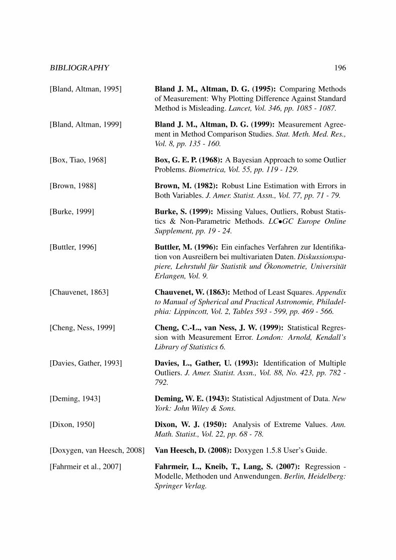
BIBLIOGRAPHY 196
[Bland, Altman, 1995] Bland J. M., Altman, D. G. (1995): Comparing Methods
of Measurement: Why Plotting Difference Against Standard
Method is Misleading. Lancet, Vol. 346, pp. 1085 - 1087.
[Bland, Altman, 1999] Bland J. M., Altman, D. G. (1999): Measurement Agree-
ment in Method Comparison Studies. Stat. Meth. Med. Res.,Vol. 8, pp. 135 - 160.
[Box, Tiao, 1968] Box, G. E. P. (1968): A Bayesian Approach to some Outlier
Problems. Biometrica, Vol. 55, pp. 119 - 129.
[Brown, 1988] Brown, M. (1982): Robust Line Estimation with Errors in
Both Variables. J. Amer. Statist. Assn., Vol. 77, pp. 71 - 79.
[Burke, 1999] Burke, S. (1999): Missing Values, Outliers, Robust Statis-
tics & Non-Parametric Methods. LC•GC Europe OnlineSupplement, pp. 19 - 24.
[Buttler, 1996] Buttler, M. (1996): Ein einfaches Verfahren zur Identifika-
tion von Ausreißern bei multivariaten Daten. Diskussionspa-piere, Lehrstuhl fur Statistik und Okonometrie, UniversitatErlangen, Vol. 9.
[Chauvenet, 1863] Chauvenet, W. (1863): Method of Least Squares. Appendixto Manual of Spherical and Practical Astronomie, Philadel-phia: Lippincott, Vol. 2, Tables 593 - 599, pp. 469 - 566.
[Cheng, Ness, 1999] Cheng, C.-L., van Ness, J. W. (1999): Statistical Regres-
sion with Measurement Error. London: Arnold, Kendall’sLibrary of Statistics 6.
[Davies, Gather, 1993] Davies, L., Gather, U. (1993): Identification of Multiple
Outliers. J. Amer. Statist. Assn., Vol. 88, No. 423, pp. 782 -792.
[Deming, 1943] Deming, W. E. (1943): Statistical Adjustment of Data. NewYork: John Wiley & Sons.
[Dixon, 1950] Dixon, W. J. (1950): Analysis of Extreme Values. Ann.Math. Statist., Vol. 22, pp. 68 - 78.
[Doxygen, van Heesch, 2008] Van Heesch, D. (2008): Doxygen 1.5.8 User’s Guide.
[Fahrmeir et al., 2007] Fahrmeir, L., Kneib, T., Lang, S. (2007): Regression -
Modelle, Methoden und Anwendungen. Berlin, Heidelberg:Springer Verlag.

BIBLIOGRAPHY 197
[Feldmann, 1992] Feldmann, U. (1992): Robust Bivariate Errors-in-Variables
Regression and Outlier Detection. Eur. J. Clin. Chem. Clin.Biochem., Vol. 30, pp. 405 - 414.
[Fishman, Moore, 1982] Fishman, G. S., Moore, L. R. (1982): A Statistical Evalu-
ation of Multiplicative Congruential Generators with Modu-
lus (231 − 1). J. Amer. Statist. Assn., Vol. 77, No. 1, pp. 29 -136.
[Fuller, 1987] Fuller, W. A. (1987): Measurement Error Models. NewYork: John Wiley & Sons.
[Goodwin, 1913] Goodwin, H. M. (1913): Elements of the Precision of Mea-
surements and Graphical Methods. New York: McGraw-Hill.
[Grubbs, 1950] Grubbs, F. E. (1950): Sample Criteria for Testing Outlying
Observations. Ann. Math. Statist., Vol. 21, pp. 27 - 58.
[Guttman, 1973] Guttman, I. (1973): Care and Handling of Univariate and
Multivariate Outliers in Detecting Spuriosity - A Baysian
Approach. Technometrics, Vol. 15, pp. 723 - 738.
[Haeckel,1993] Haeckel, R. (1993): Evaluation Methods in Laboratory
Medicine. Weinheim: VCH Verlag.
[Hartmann et al. 1996] Hartmann, C., Smeyers-Verbeke, J., Massart, D.L.(1996): Detection of Bias in Method Comparison Studies
by Regression Analysis. Anal. Chim. Act., Vol. 338, pp. 19 -40.
[Hartmann et al. 1997] Hartmann, C., Vankeerberghen, P., Smeyers-Verbeke, J.,Massart, D.L. (1997): Robust Orthogonal Regression for
the Outlier Detection when Comparing Two Series of Mea-
surement Results. Anal. Chim. Act., Vol. 344, pp. 17 - 28.
[Hartung et al., 2009] Hartung, J., Elpelt, B., Klosener, K.-H. (2009): Statistik
- Lehr- und Handbuch der angewandten Statistik. Munchen:Oldenbourg.
[Hawkins, 1980] Hawkins, D. M. (1980): Introduction to Outliers. London:Chapman & Hall.
[Hawkins, 2002] Hawkins, D. M. (2002): Diagnostics for Conformity of
Paired Quantitative Measurements. Statist. Med., Vol. 21, pp.1913 - 1935.

BIBLIOGRAPHY 198
[Hochberg, Tamhane, 1987] Hochberg, Y., Tamhane, A. C. (1987): Multiple Compari-
son Procedures. New York: John Wiley & Sons.
[Holm, 1979] Holm, S. (1979): A Simple Sequentially Rejective Multiple
Test Procedure. Stand. J. Statist., Vol. 6, pp. 65 - 70.
[Hsu, 1996] Hsu, J.C. (1996): Multiple Comparisons - Theory and
Methods. New York: Chapmann & Hall / CRC.
[Irwin, 1925] Irwin, J. O. (1925): On a Criterion for the Rejection of Out-
lying Observations. Biometrica, Vol. 17, pp. 238-250.
[Konnert, 2005] Konnert, A. (2005): Detection of Outliers in Method
Comparison Studies. Internal Report - Roche Diagnostics,Penzberg, Germany.
[Linnet, 1998] Linnet, K. (1998): Performance of Deming Regression
Analysis in Case of Misspecified Analytical Error Ratio in
Method Comparison Studies. Clin. Chim., Vol. 44, No. 5, pp.1024 - 1031.
[Linnet, 1990] Linnet, K. (1990): Estimation of the Linear Relationship
between the measurements of two Methods with Propor-
tional errors. Statist. Med., Vol. 9, pp. 1463 - 1473.
[Marks, Rao, 1979] Marks, R. G., Rao, P. V. (1979): An Estimation Procedure
for Data Containing Outliers with a One-Directional Shift in
the Mean. J. Amer. Statist. Assn., Vol. 74, pp. 614 - 620.
[Olive, 2005] Olive, D. J. (2005): Two Simple Resistant Regression Esti-
mators. Comp. Statist. Data Anal., Vol. 49, pp. 809 - 819.
[Passing, Bablok, 1983] Passing, H., Bablok, W. (1983): A New Biometrical
Procedure for Testing the Equality of Measurements from
Two Different Analytical Methods - Application of Linear
Regression Procedures for Method Comparison Studies in
Clinical Chemistry, Part I. J. Clin. Chem. Clin. Biochem.,Vol. 21, pp. 709 - 720.
[Passing, Bablok, 1984] Passing, H., Bablok, W. (1984): Comparison of Sev-
eral Regression Procedures for Method Comparison Studies
and Determination of Sample Size - Application of Linear
Regression Procedures for Method Comparison Studies in
Clinial Chemistry, Part II. J. Clin. Chem. Clin. Biochem. Vol.22, pp. 431-445.

BIBLIOGRAPHY 199
[Pearson, Sekar, 1936] Pearson, E. S., Sekar, C. C. (1936): The Efficiency of Sta-
tistical Tools and a Criterion for the Rejection of Outlying
Observations. Biometrica, Vol. 28, pp. 308 - 320.
[Peirce, 1852] Peirce, E. S. (1852): Criterion for the Rejection of Doubtful
Observations. Astron. J., Vol. 2, pp. 161 - 163.
[Qian, 1998] Qian, J. (1998): Estimation of the Effective Degrees of
Freedom in T-Type Tests for Complex Data. Proceedings ofthe Survey Research Methods Section, ASA, pp. 704 - 708.
[Rio et al., 2001] Del Rio, F. J., Riu, J., Rius, F. X. (2001): Graphical Crite-
rion for the Detection of Outliers in Linear Regression taking
Account Errors in Both Axes. Anal. Chim. Act., Vol. 446, pp.489 - 494.
[Rocke, Lorenzato, 1995] Rocke, D. M., Lorenzato, S.,(1995): A two Compo-
nent Model for Measurement Error in Analytical Chemistry.
Technometrics , Vol. 37, No. 2, pp. 176 - 184.
[Rousseeuw, Leroy, 1987] Rousseeuw, P. J., Leroy, A. M.,(1987): Robust Regression
and Outlier Detection. New York: John Wiley & Sons.
[Rousseeuw, Zomeren, 1990] Rousseeuw, P. J., van Zomeren, B. C.,(1990): Unmasking
Multivariate Outliers and Leverage Points. J. Amer. Statist.Assn., Vol. 85, No. 411, pp. 49 - 58.
[SAS Insitute Inc., 2008] SAS Insitute Inc. (2008): SAS® 9.1.3 User’s Guide.
[Satterthwaite, 1941] Satterthwaite, F. (1941): Synthesis of Variance. Psychome-trika, Vol. 6, No. 5, pp. 309 - 316.
[Satterthwaite, 1946] Satterthwaite, F. (1946): An Approximate Distribution of
Estimates of Variance Components. Biom. Bull., Vol. 2, pp.110 - 114.
[Shepard, 1968] Shepard, D. (1968): A Two-Dimensional Interpolation
Function for Irregularly-Spaced Data. Proceedings of the1968 ACM National Conference, pp. 517 - 524
[Stokl et al., 1998] Stokl, D., Dewitte, K., Thienpont, L. M. (1998): Validity
of Linear Regression in Method Comparison Studies: Is it
Limited by the Statistical Model or the Quality of the Ana-
lytical Input Data? Clin. Chem., Vol. 44, No. 11, pp. 2340 -2346.

BIBLIOGRAPHY 200
[Stone, 1868] Stone, E. J. (1868): On the Rejection of Discordant Obser-
vations. Monthly Notices Roy. Astr. Soc., Vol. 28, pp. 165 -168.
[Theil 1950] Theil, H. (1950): Proc. Kon. Ned. Akad. v. Wetensch. AS 3,Part I: pp. 386-392, Part II: pp. 521-525, Part III: pp. 1397- 1412.
[Thompson, 1935] Thompson, W.R. (1935): On a Criterion for the Rejection
of Observations and the Distribution of the Ratio of the Devi-
ation to the Sample Standard Deviation. Ann. Math. Statist.,Vol. 6, pp. 214 - 219.
[Tukey 1960] Tukey, J. W. (1960): A Survey of Sampling from Contam-
inated Distributions. In Olkin, I. (Editor) (1960): Contri-butions to Probability and Statistics, Standford, California:University Press.
[Ukkelberg, Borgen, 1993] Ukkelberg, A., Borgen, O. S. (1993): Outlier Detection by
Robust Alternating Regression. Anal. Chim. Act., Vol. 277,pp. 489 - 494.
[Wellmann, Gather, 2003] Wellmann, J., Gather, U. (2003): Identification of Outliers
in a One-Way Random Effects Model. Stat. Papers, Vol. 44,pp. 335 - 348.
[Wadsworth, 1990] Wadsworth, H. M. Jr. (1990): Handbook of Statistical
Methods for Engineers and Scientists. New York: McGraw-Hill
[Wright, 1884] Wright, T.W. (1884): A Treatise on the Adjustment of Ob-
servations by the Method of Least Squares. New York: VanNostrand
[Xie, Wei, 2003] Xie, F.-C., Wei, B.-C. (2007): Diagnostics Analysis for
Log-Birnbaum-Saunders Regression Models. Comp. Statist.Data Anal., Vol. 51, pp. 4692 - 4706.