The Long-Run Phillips Curve:

A Structural VAR Investigation∗

Luca Benati

University of Bern†

Abstract

I use structural VARs identified based on either long-run restrictions, or a

combination of long-run and sign restrictions, to investigate the long-run trade-

off between inflation and the unemployment rate in the U.S., the Euro area,

the U.K., Canada and Australia over the post-WWII period.

Results based on VARs featuring a single permanent inflation shock do not

allow to reject the null hypothesis of a vertical long-run Phillips curve for either

country. Results based on VARs allowing for four permanent inflation shocks,

which are sorted out from one another by means of DSGE-based robust sign

restrictions, produce a very similar picture. The overall extent of uncertainty

is however substantial, thus suggesting that the data are compatible with a

comparatively wide range of possible slopes of the long-run trade-off.

For all countries, Johansen’s cointegration tests point towards the presence

of cointegration between either inflation and unemployment, or inflation, un-

employment, and a short-term interest rate, with the long-run Phillips trade-off

implied by the estimated cointegrating vectors being negative and sizeable. I

argue however that this evidence should be discounted, as, conditional on the

estimated structural VARs–which, by construction, do not feature cointegra-

tion between any variable–Johansen’s procedure tends to spuriously detect

cointegration a non-negligible, and sometimes large, fraction of the times.

Keywords: Phillips curve; unit roots; cointegration; Bayesian VARs; structural

VARs; long-run restrictions; sign restrictions.

∗I wish to thank the Co-Editor (R. Reis) and an anonymous referee for extremely helpful com-ments and suggestions. Thanks to F. Canova and R. Cooper for helpful discussions; J. Carrillo,

H. Uhlig and seminar participants at CREST, the European University Institute, Norges Bank, the

Swiss National Bank’s 2012 research conference ‘Policy Challenges and Developments in Monetary

Economics’, and the 2013 Workshop on Empirical Macroeconomics held at the University of Ghent

for comments; and J. Rubio-Ramirez for helpful suggestions. Usual disclaimers apply.†Department of Economics, University of Bern, Schanzeneckstrasse 1, CH-3001 Bern, Switzer-

land. Email: luca.benati@vwi.unibe.ch

1

1 Introduction

In spite of the central role played by the unemployment-inflation trade-off in shaping

the evolution of both macroeconomic thinking1 and policymaking over the last several

decades, surprisingly little econometric work has been devoted to investigating the

nature of the long-run trade-off. In particular, as I discuss more extensively below,

to the best of my knowledge the only existing investigation of the long-run Phillips

trade-off based on structural VAR methods is King and Watson (1994)’s ‘revision-

ist econometric history’ of the post-WWII U.S. Phillips curve, which has produced

evidence of a negative, and statistically significant long-run trade-off conditional on

aggregate demand-side shocks.

In this paper I use both Classical and Bayesian structural VARs identified based

on either long-run restrictions, or a combination of long-run and sign restrictions, in

order to investigate the long-run trade-off between inflation and the unemployment

rate in the U.S., the Euro area, the U.K., Canada and Australia over the post-WWII

period.

Results based on Classical VARs featuring a single permanent inflation shock do

not allow to reject the null hypothesis of a vertical long-run Phillips curve for either

country, with both the modes and the medians of the bootstrapped distributions of

the long-run impact on unemployment of a one per cent permanent shock to inflation

being close to zero. Applying the same identification strategy within a Bayesian con-

text produces results which are numerically very close to those produced by Classical

methods, pointing, once again, towards no long-run unemployment-inflation trade-off.

Since, in principle, these results are not incompatible with the notion that some of

the shocks exerting a permanent impact on inflation may induce a non-zero long-run

Phillips trade-off, working within a Bayesian context I then proceed to disentangle

permanent inflation shocks into demand- and supply-side ones, by imposing Canova

and Paustian’s (2011) DSGE-based ‘robust sign restrictions’ on their impact on the

endogenous variables at =0. Overall, results are qualitatively similar to the one

produced by VARs featuring a single permanent inflation shock. In particular,

(i) for all countries, and for either shock, the 90%-coverage percentiles of the

posterior distributions of the long-run impact on the unemployment rate of a one per

cent permanent shock to inflation contain zero, thus implying that the notion of a

vertical long-run Phillips curve cannot be rejected at conventional significance levels.

(ii) For either shock, both the modes and the medians of the posterior distribu-

tions of the long-run impact on unemployment of a one per cent permanent shock to

inflation are, in general, close to zero.

An important point to stress, however, is that the overall extent of uncertainty is

substantial, thus suggesting that the data are compatible with a comparatively wide

range of possible slopes of the long-run trade-off. This is the case both for the Classical

and Bayesian VARs featuring a single permanent inflation shock, and, especially, for

1See in particular Lucas (1972a), Lucas (1972b), and Lucas (1973).

2

the Bayesian VARs allowing for multiple shocks exerting a permanent impact on

inflation. For the U.S., for example, the 90% bootstrapped confidence interval for the

estimated long-run impact on the unemployment rate of a one per cent permanent

shock to inflation produced by Classical VARs featuring a single permanent inflation

shock stretches between -0.56 and 0.15. The key reason for such a comparatively large

extent of uncertainy is that the feature of the data we are attempting to estimate

pertains to the infinite long run, and, as it is well known–see e.g. Faust and Leeper

(1997)–this is bound to produce imprecise estimates, unless the researcher is willing

to impose upon the data very strong restrictions (which, in general, is not advisable).

In the case of the VARs allowing for four permanent inflation shocks, this problem

is compounded by our use of sign restrictions, which, as stressed by Fry and Pagan

(2011), are intrinsically ‘weak information’, and should therefore not be expected to

produce strong inference.

For all countries, Johansen’s cointegration tests point towards the presence of

cointegration between either inflation and unemployment, or inflation, unemploy-

ment, and a short-term interest rate, with the long-run Phillips trade-off implied by

the estimated cointegrating vectors being negative and sizeable. As I show via Monte

Carlo, this is not the product of the comparatively short samples I am working with,

as the fraction of simulations for which the bootstrapped trace statistic incorrectly

rejects the null of no cointegration between two independent random walks at a given

significance level ranges between 11.3 and 11.9 per cent at the 10 per cent level; be-

tween 5.5 and 6.0 per cent at the 5 per cent level; and between 1.1 and 1.3 per cent at

the 1 per cent level, thus pointing towards an excellent performance of the cointegra-

tion procedure I am using herein (which largely originates from the bootstrap’s ability

to effectively take into account of the specific characteristics of the data generation

process under investigation). I argue however that this evidence should be discounted,

as, conditional on the estimated structural VARs–which, by construction, do not fea-

ture cointegration between any variable–Johansen’s bootstrapped procedure tends

to spuriously detect cointegration a non-negligible fraction of the times. For example,

for the Euro area and the U.K., conditional on taking the VARs featuring four per-

manent inflation shocks as data generation processes, the fractions of bootstrapped

p-values for Johansen’s trace statistic for testing the null of no cointegration between

inflation and the unemployment rate which are smaller than 10 per cent are equal to

0.269 and 0.236 per cent respectively. This means that, if the estimated structural

VARs were the true data-generation process, Johansen’s trace test would incorrectly

reject the null of no cointegration between inflation and unemployment at the 10 per

cent level about one-fourth of the times.

1.1 Related literature

To the very best of my knowledge, the only existing investigation of the long-run

Phillips trade-off based on structural VAR methods is King and Watson’s (1994)

3

‘revisionist econometric history’ of the post-WWII U.S. Phillips curve. King and

Watson (1994) estimate a bivariate VAR for the first differences of CPI inflation and

the unemployment rate for the period 1954-1992, and explore the long-run trade-

off induced by aggregate demand-side permanent shocks to inflation based on three

alternative identification schemes. Results based on the identification scheme they

regard as more reliable (which they label as ‘Rational Expectations Monetarist’) point

towards a negative, statistically significant, and comparatively flat long-run Phillips

trade-off for either the full sample period, or the 1970-1992 sub-sample (with point

estimates equal to -0.29 and -0.23, respectively), and to a steeper trade-off for the

1954-1969 sub-sample (with a point estimate of -0.47).

Nearly two decades after King and Watson (1994), there are several reasons why

it is of interest to reconsider this issue.

First, their finding of a negatively sloped, statistically significant, and compara-

tively flat long-run Phillips curve has radical implications for the conduct of monetary

policy, as it implies that the current consensus, within the central banking community,

that there is no long-run trade-off between inflation and economic activity–with its

corollary that the central bank should focus on delivering low and stable inflation–is

misplaced. Current monetary frameworks have been built around the notion that

there is no long-run trade-off which can be exploited by monetary policy: in spite of

its strong conceptual appeal, it is important to know whether such a notion is in fact

supported by empirical evidence.

Second, in the years since 1994 structural VAR econometrics has seen important

developments in terms of identification. When King and Watson wrote, short-run

restrictions were still either of the ‘inertial’ type–that is, based on imposing zeros

in the impact matrix of the structural shocks at =0–or they were based on the

notion of ‘calibrating’ some of these impacts based on information extraneous to the

VAR.2 In recent years, several contributions have highlighted the dangers associated

with the former approach,3 whereas the reliability of the latter crucially hinges, as a

matter of logic, on just how credible the numbers the researcher is imposing in the

VAR’s structural impact matrix truly are. Since imposing a specific number entails

making a very strong assumption–implying an extent of knowledge we typically

2Indeed, this is how King and Watson (1994) achieved identification in their preferred specifica-

tion. As stressed by Evans (1994) in his comment on King and Watson (1994),

‘[i]dentification of the supply and demand shocks is achieved by imposing a value for

[the parameter which determines the impact of demand shocks on the unemployment

rate at = 0] a priori in the empirical analysis.’. (See Evans, 1994, p. 222.)

3The work of Fabio Canova and his co-authors, in particular (see, first and foremost, Canova and

Pina, 2005) has demonstrated that, since inertial restrictions are, in general, incompatible with the

structure of general equilibrium models–in the specific sense that, within DSGE models, the impact

matrix of the structural shocks at =0 is, in general ‘full’, i.e., it has no zero entries–imposing such

zeros can lead to dramatically distorted inference, for example ‘uncovering’ price puzzles which are

not in the data generation process.

4

do not have–an alternative style of identification based on weaker informational

requirements might be regarded as preferrable. Several researchers4 have therefore

proposed sign restrictions–that is, restrictions on the signs of the impacts of the

structural shocks at =0, and possibly on their impulse-response functions at longer

horizons–as the best (or least bad ...) way of achieving identification based on short-

run restrictions. As shown by Canova and Paustian (2011), indeed, DSGE models

often imply a robust pattern of signs for the impacts of the structural shocks at

=0 (where ‘robust’ means that such pattern holds true for alternative sub-classes of

DSGE models, and for a wide range of plausible parameters’ configurations), which is

often sufficient to disentangle the structural shocks from one another. In fact, when

seen from the perspective of DSGE models, a specific pattern of signs for the impacts

of the structural shocks at =0 is typically the only kind of information we can be

reasonably confident about, whereas the specific values taken by such impacts are, in

general, much more uncertain, thus raising doubts on the reliability of an approach

to identification based on the notion of calibrating such impacts.5

Third, King and Watson’s analysis was entirely based on a bivariate VAR for

the first differences of inflation and the unemployment rate, but, as shown by Evans

(1994) in his comment,6 even based on their identification strategy, evidence based on

trivariate VARs was sometimes significantly different, pointing in some cases towards

a vertical long-run Phillips curve. This naturally suggests reconsidering the issue

based on VARs featuring a broader informational content, in particular about the

stance of monetary policy and the state of the business cycle.7

2 Three Alternative Forms of the Long-Run Phillips

Curve

In what follows we consider three alternative forms of the long-run Phillips curve

(henceforth, LRPC).

4See in particular Faust (1998), Canova and de Nicolo’ (2002), and Uhlig (2005).5An approach to identification based on sign restrictions is not without problems of its own.

As extensively discussed by Fry and Pagan (2011), in particular, sign restrictions suffers from the

shortcoming that they are intrinsically ‘weak information’, and therefore they should not be expected

to produce strong inference.6See Evans (1994, Section 3.2, and in particular the results reported in Figure 2).7For the reason discussed, e.g., by Sargent (1987)–that is: the first-difference filter wipes out

most of the variance at the business-cycle frequencies–the fact that, as it is well known, the level of

the U.S. unemployment rate is highly informative about the state of the U.S. business cycle logically

implies that its first difference is not. This means that a VAR for the U.S. which, beyond the first-

difference of the unemployment rate, does not include other indicators of real economic activity,

does not contain strong information about the state of the business cycle.

5

2.1 A strong-form LRPC

First, we consider a ‘strong form of the LRPC’, in which inflation and the unem-

ployment rate are (possibly) cointegrated. Such a strong form implies that (i) all

shocks having a permanent impact on inflation also have a permanent impact on the

unemployment rate (and vice versa), and (ii) for either of these shocks, the ratio

between the long-run impacts on the two variables is exactly the same (thus implying

that inflation and unemployment share the same stochastic trend across all possible

shocks).

We investigate whether the data are consistent with such a strong from of the

LRPC via standard cointegration methods.

2.2 A medium-form LRPC

Since either (i) or (ii) may well be violated, we also consider two weaker forms

of the LRPC, starting from a ‘medium-form LRPC’ conceptually in line with King

and Watson (1994), in which the unit root component of the unemployment rate is

driven by both idiosyncratic shocks, and permanent shocks to inflation. It is not

difficult to think of circumstances under which this may be the case. For example,

permanent shocks to the tax rate on labor should lead to increases in the natural

rate of unemployment, but–being shocks to the level of the tax rate, as opposed to

its rate of change–they should only have a transitory impact on inflation. By the

same token, given the widely documented stylized fact that unemployment rates differ

systematically by age/sex/race groups, secular changes in the composition of the labor

force should lead to permanent changes in the overall natural rate of unemployment,

but at the same time they should not have any permanent impact on inflation. So

the bottom line is that it is pretty easy to think of circumstances in which the strong

form of the LRPC does not hold, but the medium-form may hold.

In the spirit of King and Watson (1994), in what follows we will search for a

medium-form LRPC based on structural VARs featuring, beyond the first differences

of inflation and unemployment, a measure of the output gap, the consumption/GDP

ratio, a long-short spread, and (the first difference of) the short-term monetary pol-

icy rate. These variables effectively expand the informational content of King and

Watson’s original bivariate VAR along several dimensions. The short rate and, to a

lesser extent, the long-short spread contain information about the monetary policy

stance. As recently shown by Kurmann and Otrok (2013), the long-short spread pos-

sesses a strong informational content for future movements in technology. Finally, the

consumption/GDP ratio and the output gap measure can be regarded as two ‘noisy

estimates’ of the state of the business cycle. We consider these additional variables

for two reasons. First, King and Watson’s analysis was entirely based on a bivariate

VAR for the first differences of inflation and the unemployment rate, but, as shown

by Evans (1994) in his comment, even based on their identification strategy, evidence

based on trivariate VARs was sometimes significantly different, pointing in some cases

6

towards a vertical long-run Phillips curve. Second, as recently discussed by Forni and

Gambetti (2014), small VARs with a limited informational content may well produce

unreliable results. We will identify a single, ‘aggregate’ permanent inflation shock via

standard long-run restrictions, and we will then explore whether such a shock has a

non-zero long-run impact on the unemployment rate.

2.3 A weak-form LRPC

Since, in principle, absence of a long-run trade-off conditional on such ‘aggregate’

permanent inflation shock is not incompatible with the notion that some of the shocks

exerting a permanent impact on inflation may induce a non-vertical LRPC, we then

proceed to explore a ‘weak-form LRPC’, in which either of these shocks is allowed to

give rise to an idiosyncratic trade-off. Specifically, we disentangle permanent inflation

shocks into demand- and supply-side ones by imposing Canova and Paustian’s (2011)

DSGE-based ‘robust sign restrictions’ on their impact on the endogenous variables

at =0, and we proceed to explore whether any of these shocks has a statistically

significant long-run impact on the unemployment rate. Although we identify four

different shocks having a permanent impact on inflation, we mostly focus upon shocks

of a monetary nature. The reason for doing so is that the motivation behind all

explorations of the slope of the LRPC has always been understanding whether the

monetary authority might be able to permanently lower the unemployment rate by

engineering a permanently higher rate of inflation. Under this respect, the long-run

Phillips trade-offs which might originate from permanent inflation shocks of a non-

monetary nature are therefore irrelevant. The framework used in order to explore the

weak-form LRPC has an obvious connection to the one used to explore the medium-

form one. Whereas, by construction, the permanent inflation shocks identified by

the ‘medium-form LRPC’ VAR explain 100 per cent of the infinite long-run variance

of inflation, the four permanent inflation shocks identified by the ‘weak-form LRPC’

VAR jointly explain all of the long-run variance of inflation (in particular, in most

cases permanent inflation shocks of a monetary nature are essentially negligible).

3 The Data

As discussed by King and Watson (1994), the possibility of identifying the long-run

impact on the unemployment rate of permanent inflation shocks crucially hinges on

the fact that both series contain an I(1) component. As documented by Benati (2008),

however, evidence of high inflation persistence is weak-to-non-existent for all sample

periods which are not dominated by the Great Inflation episode (and especially so for

monetary regimes such as inflation targeting). In what follows I therefore consider the

following sample periods: for the Euro area, 1970Q1-1998Q4 (EMU started in January

1999, whereas Euro area data are only available starting from 1970Q1); for the U.K.,

1972Q2-1992Q3 (June 1972 marks the floating of the pound vis-à-vis the U.S. dollar,

7

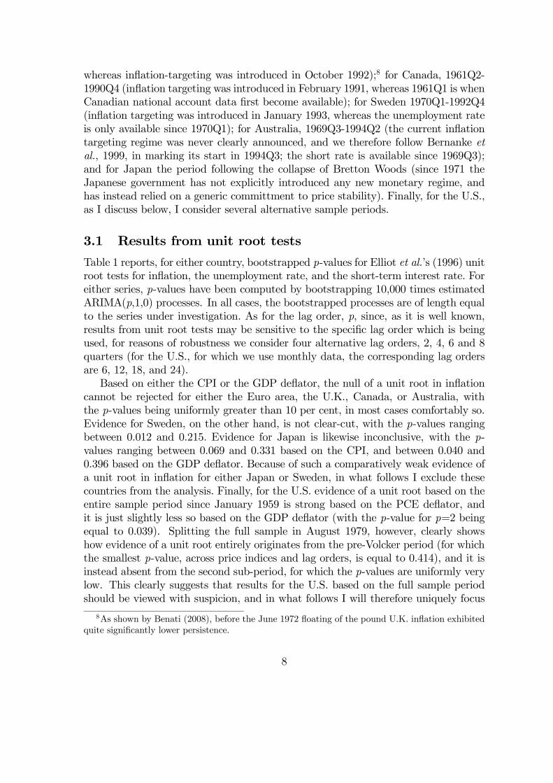
whereas inflation-targeting was introduced in October 1992);8 for Canada, 1961Q2-

1990Q4 (inflation targeting was introduced in February 1991, whereas 1961Q1 is when

Canadian national account data first become available); for Sweden 1970Q1-1992Q4

(inflation targeting was introduced in January 1993, whereas the unemployment rate

is only available since 1970Q1); for Australia, 1969Q3-1994Q2 (the current inflation

targeting regime was never clearly announced, and we therefore follow Bernanke et

al., 1999, in marking its start in 1994Q3; the short rate is available since 1969Q3);

and for Japan the period following the collapse of Bretton Woods (since 1971 the

Japanese government has not explicitly introduced any new monetary regime, and

has instead relied on a generic committment to price stability). Finally, for the U.S.,

as I discuss below, I consider several alternative sample periods.

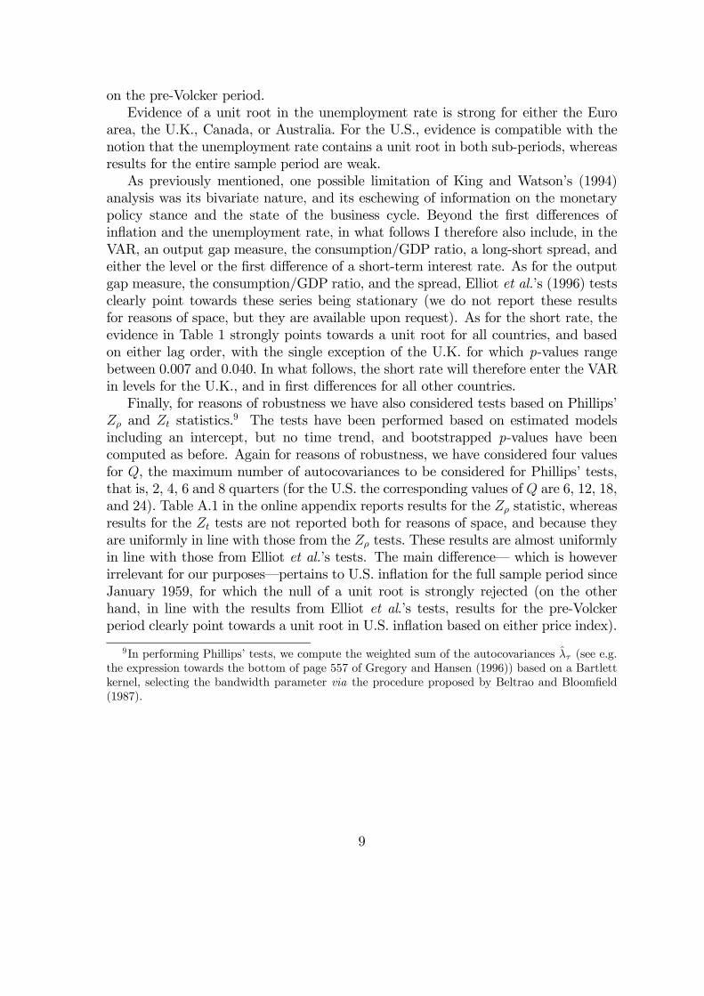
3.1 Results from unit root tests

Table 1 reports, for either country, bootstrapped p-values for Elliot et al.’s (1996) unit

root tests for inflation, the unemployment rate, and the short-term interest rate. For

either series, p-values have been computed by bootstrapping 10,000 times estimated

ARIMA(p,1,0) processes. In all cases, the bootstrapped processes are of length equal

to the series under investigation. As for the lag order, p, since, as it is well known,

results from unit root tests may be sensitive to the specific lag order which is being

used, for reasons of robustness we consider four alternative lag orders, 2, 4, 6 and 8

quarters (for the U.S., for which we use monthly data, the corresponding lag orders

are 6, 12, 18, and 24).

Based on either the CPI or the GDP deflator, the null of a unit root in inflation

cannot be rejected for either the Euro area, the U.K., Canada, or Australia, with

the p-values being uniformly greater than 10 per cent, in most cases comfortably so.

Evidence for Sweden, on the other hand, is not clear-cut, with the p-values ranging

between 0.012 and 0.215. Evidence for Japan is likewise inconclusive, with the p-

values ranging between 0.069 and 0.331 based on the CPI, and between 0.040 and

0.396 based on the GDP deflator. Because of such a comparatively weak evidence of

a unit root in inflation for either Japan or Sweden, in what follows I exclude these

countries from the analysis. Finally, for the U.S. evidence of a unit root based on the

entire sample period since January 1959 is strong based on the PCE deflator, and

it is just slightly less so based on the GDP deflator (with the p-value for p=2 being

equal to 0.039). Splitting the full sample in August 1979, however, clearly shows

how evidence of a unit root entirely originates from the pre-Volcker period (for which

the smallest p-value, across price indices and lag orders, is equal to 0.414), and it is

instead absent from the second sub-period, for which the p-values are uniformly very

low. This clearly suggests that results for the U.S. based on the full sample period

should be viewed with suspicion, and in what follows I will therefore uniquely focus

8As shown by Benati (2008), before the June 1972 floating of the pound U.K. inflation exhibited

quite significantly lower persistence.

8

on the pre-Volcker period.

Evidence of a unit root in the unemployment rate is strong for either the Euro

area, the U.K., Canada, or Australia. For the U.S., evidence is compatible with the

notion that the unemployment rate contains a unit root in both sub-periods, whereas

results for the entire sample period are weak.

As previously mentioned, one possible limitation of King and Watson’s (1994)

analysis was its bivariate nature, and its eschewing of information on the monetary

policy stance and the state of the business cycle. Beyond the first differences of

inflation and the unemployment rate, in what follows I therefore also include, in the

VAR, an output gap measure, the consumption/GDP ratio, a long-short spread, and

either the level or the first difference of a short-term interest rate. As for the output

gap measure, the consumption/GDP ratio, and the spread, Elliot et al.’s (1996) tests

clearly point towards these series being stationary (we do not report these results

for reasons of space, but they are available upon request). As for the short rate, the

evidence in Table 1 strongly points towards a unit root for all countries, and based

on either lag order, with the single exception of the U.K. for which p-values range

between 0.007 and 0.040. In what follows, the short rate will therefore enter the VAR

in levels for the U.K., and in first differences for all other countries.

Finally, for reasons of robustness we have also considered tests based on Phillips’

and statistics.9 The tests have been performed based on estimated models

including an intercept, but no time trend, and bootstrapped p-values have been

computed as before. Again for reasons of robustness, we have considered four values

for , the maximum number of autocovariances to be considered for Phillips’ tests,

that is, 2, 4, 6 and 8 quarters (for the U.S. the corresponding values of are 6, 12, 18,

and 24). Table A.1 in the online appendix reports results for the statistic, whereas

results for the tests are not reported both for reasons of space, and because they

are uniformly in line with those from the tests. These results are almost uniformly

in line with those from Elliot et al.’s tests. The main difference– which is however

irrelevant for our purposes–pertains to U.S. inflation for the full sample period since

January 1959, for which the null of a unit root is strongly rejected (on the other

hand, in line with the results from Elliot et al.’s tests, results for the pre-Volcker

period clearly point towards a unit root in U.S. inflation based on either price index).

9In performing Phillips’ tests, we compute the weighted sum of the autocovariances (see e.g.

the expression towards the bottom of page 557 of Gregory and Hansen (1996)) based on a Bartlett

kernel, selecting the bandwidth parameter via the procedure proposed by Beltrao and Bloomfield

(1987).

9

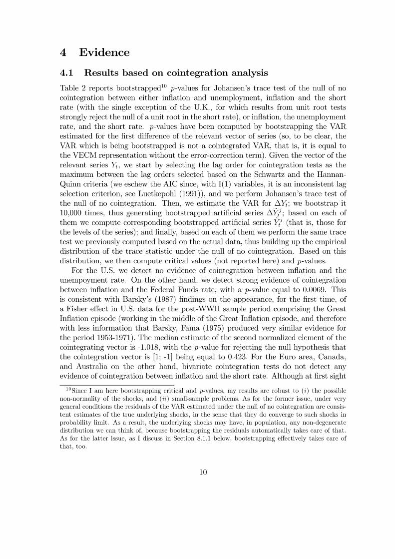
4 Evidence

4.1 Results based on cointegration analysis

Table 2 reports bootstrapped10 p-values for Johansen’s trace test of the null of no

cointegration between either inflation and unemployment, inflation and the short

rate (with the single exception of the U.K., for which results from unit root tests

strongly reject the null of a unit root in the short rate), or inflation, the unemployment

rate, and the short rate. p-values have been computed by bootstrapping the VAR

estimated for the first difference of the relevant vector of series (so, to be clear, the

VAR which is being bootstrapped is not a cointegrated VAR, that is, it is equal to

the VECM representation without the error-correction term). Given the vector of the

relevant series , we start by selecting the lag order for cointegration tests as the

maximum between the lag orders selected based on the Schwartz and the Hannan-

Quinn criteria (we eschew the AIC since, with I(1) variables, it is an inconsistent lag

selection criterion, see Luetkepohl (1991)), and we perform Johansen’s trace test of

the null of no cointegration. Then, we estimate the VAR for ∆; we bootstrap it

10,000 times, thus generating bootstrapped artificial series ∆ ; based on each of

them we compute corresponding bootstrapped artificial series (that is, those for

the levels of the series); and finally, based on each of them we perform the same trace

test we previously computed based on the actual data, thus building up the empirical

distribution of the trace statistic under the null of no cointegration. Based on this

distribution, we then compute critical values (not reported here) and p-values.

For the U.S. we detect no evidence of cointegration between inflation and the

unempoyment rate. On the other hand, we detect strong evidence of cointegration

between inflation and the Federal Funds rate, with a p-value equal to 0.0069. This

is consistent with Barsky’s (1987) findings on the appearance, for the first time, of

a Fisher effect in U.S. data for the post-WWII sample period comprising the Great

Inflation episode (working in the middle of the Great Inflation episode, and therefore

with less information that Barsky, Fama (1975) produced very similar evidence for

the period 1953-1971). The median estimate of the second normalized element of the

cointegrating vector is -1.018, with the p-value for rejecting the null hypothesis that

the cointegration vector is [1; -1] being equal to 0.423. For the Euro area, Canada,

and Australia on the other hand, bivariate cointegration tests do not detect any

evidence of cointegration between inflation and the short rate. Although at first sight

10Since I am here bootstrapping critical and p-values, my results are robust to (i) the possible

non-normality of the shocks, and (ii) small-sample problems. As for the former issue, under very

general conditions the residuals of the VAR estimated under the null of no cointegration are consis-

tent estimates of the true underlying shocks, in the sense that they do converge to such shocks in

probability limit. As a result, the underlying shocks may have, in population, any non-degenerate

distribution we can think of, because bootstrapping the residuals automatically takes care of that.

As for the latter issue, as I discuss in Section 8.1.1 below, bootstrapping effectively takes care of

that, too.

10

puzzling–taken at face value, these results imply a rejection of the Fisher hypothesis

that permanent shifts in inflation should map one-to-one into corresponding shifts in

interest rates–it ought to be stressed that empirical evidence on the violation of the

Fisher hypothesis is widespread (after all, the key reason why Fama’s (1975) paper

had such a resonance was precisely because it produced, for the first time, decisive

evidence in favor of the Fisher effect). This implies that these results should not

be seen as surprising at all. Finally, for either the U.S., the Euro area or, Canada

we detect strong evidence of cointegration between inflation, unemployment, and the

short rate, whereas for the U.K. evidence points, at the 10 per cent level, towards

cointegration between inflation and the unemployment rate.

For the U.S., the Euro area and Canada, for which we detected evidence of coin-

tegration between the three series, we also report bootstrapped p-values for testing

the null hypothesis of one single cointegrating vector, versus the alternative of two

cointegrating vectors. Details of the bootstrapping procedure are the same as before,

with the only difference that, instead of bootstrapping the estimated VAR for ∆under the null of no cointegration, we bootstrap the VECM estimated conditional

on there being one single cointegrating vector. Whereas the p-value for Canada, at

0.2896, is very far from being significant at any conventional level, those for the Euro

area and the U.S., at 0.0531 and 0.0728, respectively, point towards the presence of

an additional cointegrating vector at the 10 per cent level.

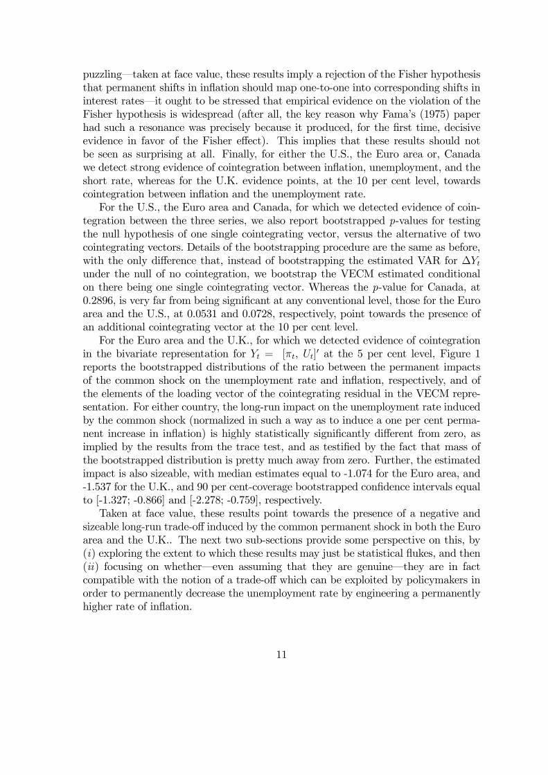
For the Euro area and the U.K., for which we detected evidence of cointegration

in the bivariate representation for = [, ]0 at the 5 per cent level, Figure 1

reports the bootstrapped distributions of the ratio between the permanent impacts

of the common shock on the unemployment rate and inflation, respectively, and of

the elements of the loading vector of the cointegrating residual in the VECM repre-

sentation. For either country, the long-run impact on the unemployment rate induced

by the common shock (normalized in such a way as to induce a one per cent perma-

nent increase in inflation) is highly statistically significantly different from zero, as

implied by the results from the trace test, and as testified by the fact that mass of

the bootstrapped distribution is pretty much away from zero. Further, the estimated

impact is also sizeable, with median estimates equal to -1.074 for the Euro area, and

-1.537 for the U.K., and 90 per cent-coverage bootstrapped confidence intervals equal

to [-1.327; -0.866] and [-2.278; -0.759], respectively.

Taken at face value, these results point towards the presence of a negative and

sizeable long-run trade-off induced by the common permanent shock in both the Euro

area and the U.K.. The next two sub-sections provide some perspective on this, by

(i) exploring the extent to which these results may just be statistical flukes, and then

(ii) focusing on whether–even assuming that they are genuine–they are in fact

compatible with the notion of a trade-off which can be exploited by policymakers in

order to permanently decrease the unemployment rate by engineering a permanently

higher rate of inflation.

11

4.1.1 Monte Carlo evidence on the performance of Johansen’s procedure

The case of two independent random walks A first possibility is that the re-

sults for the Euro area and the U.K. are a statistical fluke due to the bad performance

of Johansen’s procedure in small-samples. In order to assess this possiblity we con-

sider five sets of 10,000 Monte Carlo simulations of lengths equal to the actual sample

lengths we are working with for the five countries. For each simulation, we randomly

generate two independent random walks, and we apply exactly the same procedure

we previously applied to the actual data, computing the p-values by bootstrapping

the estimated VAR for the first differences of the two random walks. Ideally, out of

the 10,000 simulations, the fraction of bootstrapped p-values below x per cent should

be equal to x per cent. As the results reported in Table A.2 in the online appendix

clearly show, the bootstrapped Johansen procedure we are using herein gets quite

remarkably close to this ideal: the fraction of simulations for which the bootstrapped

trace statistic incorrectly rejects the null of no cointegration between the two inde-

pendent random walks at a given significance level ranges between 11.3 and 11.9 per

cent at the 10 per cent level; between 5.5 and 6.0 per cent at the 5 per cent level;

and between 1.1 and 1.3 per cent at the 1 per cent level. Quite remarkably, the

performance for the U.K., for which we have just 81 quarterly observations, is not

dramatically different from that for Canada, for which we have instead 118 observa-

tions. This testifies to the power of bootstrapping, which can effectively take into

account of the specific characteristics of the data the researcher is working with.

Taking the non-cointegrated structural VARs as data-generation processes

Although the bootstrapped Johansen procedure used herein performs remarkably

well conditional on a data-generation process (henceforth, DGP) in which the series

of interest are independent random walks, it is an open question how well such a

procedure performs conditional on DGPs such as the non-cointegrated structural

VARs featuring permanent inflation shocks we will estimate in Sections 4.2 and 4.3,

respectively. Since these results will produce no evidence whatsoever of a long-run

Phillips trade-off conditional on any kind of permanent inflation shock, it is of interest

to explore the performance of Johansen’s procedure conditional on these DGPs. To

put it differently, suppose that these structural VARs are, for either country, the

true model of the economy: how often would the Johansen procedure incorrectly

reject the null of no cointegration? Table 3 reports evidence on this, by showing the

fraction of simulations for which Johansen’s bootstrapped trace statistic incorrectly

rejects the null of no cointegration at a given significance level, based on taking the

estimated structural VARs as the DGPs. As the tables shows, Johansen’s procedure

tends to spuriously detect cointegration a non-negligible fraction of the times. Taking

the estimated Bayesian structural VARs featuring four permanent inflation shocks as

DGPs, for example, for the Euro area and the U.K., the fractions of bootstrapped

p-values for Johansen’s trace statistic for testing the null of no cointegration between

12

inflation and the unemployment rate which are smaller than 10 per cent are equal to

26.9 and 23.6 per cent respectively. This means that the trace test would incorrectly

reject the null of no cointegration between inflation and unemployment at the 10

per cent level about one-fourth of the times. As for the trace test of cointegration

between inflation, unemployment, and the short rate, the fraction of bootstrapped p-

values smaller than 10 per cent range between 45.4 and 72.1 per cent, thus essentially

pointing towards the unreliability of such tests conditional on these DGPs. Results

based on taking Bayesian VARs featuring a single permanent inflation shock as the

DGP are in line with those discussed so far for the trace test of cointegration between

inflation, unemployment, and the short rate, and are instead significantly better for

the test of cointegration between inflation and unemployment.

Overall, these results suggest that evidence such as that reported in Table 2 should

be discounted, as these results might as well be due to the limitations of cointegration

tests conditional on these specific DGPs.

4.1.2 The adjustment dynamics implied by the estimated loading vectors

Even ignoring the results reported in Table 3, the evidence shown in the last two

columns of Figure 1 is however hardly compatible with the notion of an exploitable

long-run Phillips trade-off, that is, a trade-off which a policymaker might be able to

purposefully use in order to permanently decrease the unemployment rate by engi-

neering a higher equilibrium inflation rate. As pointed out by Evans (1994, p. 222)

in his comment on King and Watson (1994),

‘[...] for a trade-off to be viewed as exploitable, a decision-maker

must have confidence that unemployment can be reduced by engineer-

ing a higher rate of inflation [...] It would be of little comfort to many

politicians if the Phillips curve trade-off simply implied that if unemploy-

ment instead turned higher, at least inflation would be lower.’

The bootstrapped distributions of the estimates of the elements of the loading

vector of the error-correction term in the VECM reported in Figure 1, however, clearly

point towards the latter case, with the estimated loading on the first difference of the

unemployment rate being extremely small for either country, and, in the case of the

Euro area, being insignificantly different from zero at conventional levels (for the U.K.,

on the other hand, it is statistically significant at the 10 per cent level, but not at

the 5 per cent level). This implies that, following a shock to the common stochastic

trend, the bulk of the dynamic adjustment to disequilibrium takes place through

movements in inflation, rather than via movements in the unemployment rate. This

is difficult to reconcile with the notion of an exploitable Phillips trade-off, and might

instead be compatible (e.g.) with the notion that, in either country, policymakers

engineered sharp recessions in order to put an end to the Great Inflation. In turn,

13

such recessions caused permanent increases in the unemployment rate via hysteresis

effects, and inflation came down gradually.

Let us now turn to the evidence produced by non-cointegrated structural VARs

featuring a single permanent inflation shock.

4.2 Evidence from non-cointegrated SVARs featuring a sin-

gle permanent inflation shock

We start by considering either Classical or Bayesian VARs featuring a single perma-

nent inflation shock. For either country we estimate the VAR(p) model

= 0 +1−1 + +− + [0] = Ω (1)

where ≡ [, ∆, ∆, ∆, ]0 for the Euro area, Canada, and Australia, and

≡ [,∆,∆, , , ]0 for the U.K., with , , , , , and being the

output gap, inflation, the unemployment rate, the short rate, the consumption/GDP

ratio, and the long-short spread, respectively. These variables effectively expand the

informational content of King and Watson’s original bivariate VAR along several

dimensions. The short rate and, to a lesser extent, the long-short spread contain

information about the monetary policy stance. As recently shown by Kurmann and

Otrok (2013), the long-short spread possesses a strong informational content for future

movements in technology. Finally, the consumption/GDP ratio and the output gap

estimate can be regarded as two ‘noisy estimates’ of the state of the business cycle

(as for the consumption/GDP ratio, see Cochrane’s (1994) extensive discussion on

this).

The U.S. is the only country for which Johansen’s trace test produces evidence

of cointegration between the short rate and inflation (see Table 2), with the boot-

strapped, bias-corrected estimate of the second element of the cointegrating vector

being equal to -1.018, and with a p-value of 0.423 for rejecting the null hypothesis

that it is equal to -1. For the U.S. I therefore set ≡ [, ∆, ∆, , -, ]0,

where - is the ex post real rate. For the Euro area, Canada, and the U.K. I set the

lag order to p=4. For the U.S., for which I work at the monthly frequency, I set it to

p=12. I identify the permanent inflation shock based on the restriction that it is the

only shock impacting upon inflation in the infinite long run. This is tantamount to

imposing that in the second row of the long-run impact matrix ∞ ≡ [−(1)]−10,where 0 is the structural shocks’ impact matrix, all of the elements except the first

one are equal to zero, so that the first element of =−10 is the permanent inflation

shock.11

11Roberts (1993) estimated a VAR for the U.S. for the first differences of inflation and the unem-

ployment rate, and the logarithm of M 2 velocity, and identified two permanent shocks to inflation

and the unemployment rate, respectively, by imposing the restrictions that they are the only shocks

impacting either variable in the long run. A key difference between Roberts (1993) and the present

work is that he imposed orthogonality between the two shocks (that is, he imposed a vertical long-

14

4.2.1 Classical estimation

Working within a Classical context, I estimate (1) via OLS based on the standard

formulas found in Luetkepohl (1991). Concerning the estimation of the impact matrix

of the structural shocks, as extensively discussed by Christiano et al. (2006), reliably

estimating ∞ requires a good estimate of the spectral density of at the frequency = 0, (0) = ∞ 0

∞, an object which VARs, given their focus on fitting the short-run dynamics of the data, should not necessarily be expected to capture well. Follow-

ing Christiano et al. (2006) we therefore consider, beyond the standard estimator of

(0) produced by the VAR–that is, (0) = [ − (1)]−1 [ − (1)]−10,

where is the estimated covariance matrix of the VAR’s reduced-form innovations–

the estimator produced by the Bartlett estimate of the spectral density matrix (see

Hamilton (1994)).

We use standard bootstrapping techniques in order to both bias-correct the es-

timated long-run impacts of the permanent inflation shock as in Kilian (1998), and

characterise the extent of uncertainty around the bias-corrected estimates (so, to be

clear, the only difference between Kilian’s (1998) paper and the present work is that

he dealt with the bias-correction of IRFs, whereas we are here bias-correcting the

long-run impacts of the structural shocks). Specifically, we bootstrap the estimated

reduced-form VAR 10,000 times, and based on each bootstrap replication we esti-

mate a VAR(p); we impose the same identification scheme we imposed on the VAR

estimated based on the actual data; and we compute the implied long-run impact

on the unemployment rate of the permanent inflation shock. Then, we use such

bootstrapped distributions, first, to bias-correct the simple estimate of the long-run

impact; and second, to characterise the extent of uncertainty surrounding such bias-

corrected estimates, by simply rescaling the original bootstrapped distribution in such

a way that its median be equal to the bias-corrected estimate (in general, however,

the extent of the bias is very small, so that, in the end, bias-correcting does not make

a material difference to the results).

4.2.2 Bayesian estimation

Working within a Bayesian context, we estimate (1) as in Uhlig (1998, 2005). Specifi-

cally, we exactly followUhlig (1998, 2005) in terms of both distributional assumptions–

the distributions for the VAR’s coefficients and their covariance matrix are postulated

to belong to the Normal-Wishart family–and of priors. For estimation details the

reader is therefore referred to either the Appendix of Uhlig (1998), or to Appendix B

of Uhlig (2005). Finally, for each estimated VAR we consider 10,000 draws from the

posterior distribution of the VAR’s coefficients and covariance matrix of innovations

(the draws are computed exactly as in Uhlig (1998, 2005)).

run Phillips curve). See also Bullard and Keating (1995), who, working with bivariate VARs for the

first difference of inflation and either output growth, or its first difference, use the same restriction

used herein in order to identify permanent inflation shocks.

15

4.2.3 Evidence

Since, for either country, results are very close both across econometric methodologies

(Classical versus Bayesian) and, within the Classical approach, for the two alternative

estimators of the spectral density matrix of the VAR at = 0, in what follows we only

report and discuss those produced by the Bayesian approach. The online appendix

however reports the entire set of results (see Figure A.3, and Table A.3).

Figure 2 shows, for either country, the distribution of the long-run impacts on the

unemployment rate of a one per cent permanent shock to inflation, together with the

distribution of the fraction of the permanent component of unemployment which is

explained by the permanent inflation shock. Table 4 reports the median and the 90%-

coverage percentiles of the distribution of the long-run impact on the unemployment

rate of a one per cent permanent shock to inflation, together with the fractions of the

mass of the distribution for which the impact is estimated to be negative.

Results are uniformly consistent across countries, and for neither of them do they

allow to reject the ‘natural’ null hypothesis of a vertical long-run Phillips curve. In

particular, for either country the 90 per cent confidence interval for the estimated

long-run impact on unemployment of a permanent inflation shock contains zero, and

the fraction of the mass of the posterior distribution for which the impact is estimated

to be negative is uniformly greater than standard levels of statistical significance, thus

highlighting how the null hypothesis of a vertical long-run Phillips curve cannot be

rejected at conventional levels. Further, for either country the posterior distribution of

the fraction of the permanent component of the unemployment rate which is explained

by permanent inflation shocks is clustered towards zero, thus implying that such

shocks explain very little of the unit root component of unemployment, and providing

additional evidence in support of the notion that the long-run Phillips curve is indeed

vertical.12

A researcher looking for evidence of a negative long-run trade-off may find some

limited support from the results for the U.S. and Canada, for which the fraction of

draws from the posterior for which the long-run impact is estimated to be negative

is slightly above 80 per cent. Although far from standard levels of statistical signifi-

cance, still, this provides some support to the notion of a negative long-run trade-off.

Further, the median estimate of the long-run impact for the U.S., at -0.27, implies

that a permanent increase in inflation by 10 percentage points would permanently

decrease the unemployment rate by 2.7 per cent, a non-negligible amount. It is fair

to say, however, that the overall picture emerging from Table 2 and Figure 2 (and

from Table A.2 and Figure A.2) points towards no long-run trade-off. For the other

four countries, for example, the median estimates of the permanent decrease in the

unemployment rate associated with a permanent increase in inflation by 10 percent-

12By definition, a vertical long-run Phillips curve implies that the fraction of the permanent

component of the unemployment rate which is explained by the permanent inflation shock is equal

to zero.

16

age points range between -0.4 and -1.3 per cent. Even if we were willing to believe

that the median estimates capture the authentic unemployment-inflation trade-offs

out there, these are hardly trade-offs which might induce policymakers to ‘try to play

the Phillips curve’.

4.3 Evidence onmonetary policy shocks from non-cointegrated

SVARs featuring four permanent inflation shock

Since, in principle, the results discussed in the previous section are not incompatible

with the notion that some of the shocks exerting a permanent impact on inflation

may induce a non-vertical long-run Phillips trade-off, working within a Bayesian

context we then proceed to disentangle permanent inflation shocks into demand- and

supply-side ones, by imposing Canova and Paustian’s (2011) DSGE-based ‘robust

sign restrictions’ on their impact on the endogenous variables at =0.13 As we will

discuss, even doing this it is not possible to find any evidence that there exists at

least one type of shock which may induce a non-vertical long-run Phillips trade-off.

4.3.1 Identification

Our identification strategy is based on the combination of long-run and sign restric-

tions. We start by separating the VAR’s structural shocks into two sets, depending

on the fact that they do, or they do not have a permanent impact on inflation. Let

the structural VAR(p) model be given by

= 0 +1−1 + +− +0 (2)

where defined as before; 0 being the impact matrix of the structural shocks at =

0; and ≡ [ , , ,

, 0 ]0 being the structural shocks, which, as standardpractice, are assumed to be unit-variance and orthogonal to one another, with ,

, ,

being Canova and Paustian’s (2011) ‘technology’, ‘monetary policy’,

‘taste’, and ‘markup’ shocks (to be discussed shortly), which are here allowed to

exert a permanent impact on inflation, and being instead a 2×1 vector of shockswhich, by construction, have a transitory impact on inflation. The second row of the

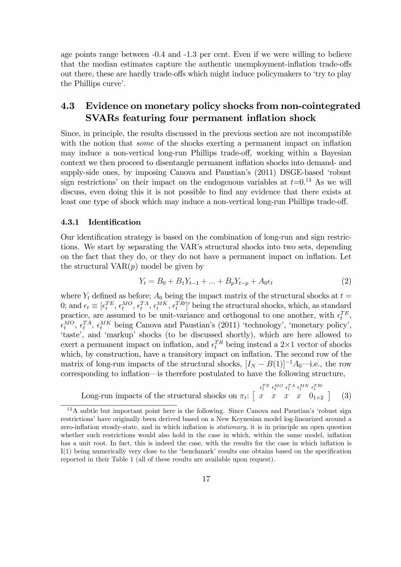
matrix of long-run impacts of the structural shocks, [ − (1)]−10–i.e., the rowcorresponding to inflation–is therefore postulated to have the following structure,

Long-run impacts of the structural shocks on :

0£

01×2¤

(3)

13A subtle but important point here is the following. Since Canova and Paustian’s ‘robust sign

restrictions’ have originally been derived based on a New Keynesian model log-linearized around a

zero-inflation steady-state, and in which inflation is stationary, it is in principle an open question

whether such restrictions would also hold in the case in which, within the same model, inflation

has a unit root. In fact, this is indeed the case, with the results for the case in which inflation is

I(1) being numerically very close to the ‘benchmark’ results one obtains based on the specification

reported in their Table 1 (all of these results are available upon request).

17

–where a ‘0’ means that the corresponding long-run impact has been restricted to

zero, whereas an ‘’ means that it has been left unrestricted–thus implying that ,

, , and

may have a permanent impact on inflation, whereas does not.

The restriction that the two shocks in are the only shocks which do not have a

permanent impact on inflation is sufficient to disentangle them from the other four

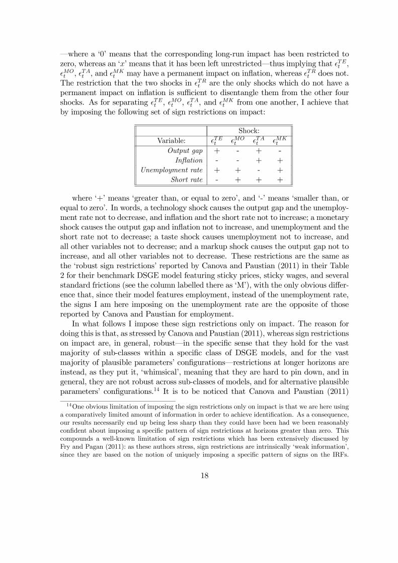
shocks. As for separating , , , and

from one another, I achieve that

by imposing the following set of sign restrictions on impact:

Shock:

Variable:

Output gap + - + -

Inflation - - + +

Unemployment rate + + - +

Short rate - + + +

where ‘+’ means ‘greater than, or equal to zero’, and ‘-’ means ‘smaller than, or

equal to zero’. In words, a technology shock causes the output gap and the unemploy-

ment rate not to decrease, and inflation and the short rate not to increase; a monetary

shock causes the output gap and inflation not to increase, and unemployment and the

short rate not to decrease; a taste shock causes unemployment not to increase, and

all other variables not to decrease; and a markup shock causes the output gap not to

increase, and all other variables not to decrease. These restrictions are the same as

the ‘robust sign restrictions’ reported by Canova and Paustian (2011) in their Table

2 for their benchmark DSGE model featuring sticky prices, sticky wages, and several

standard frictions (see the column labelled there as ‘M’), with the only obvious differ-

ence that, since their model features employment, instead of the unemployment rate,

the signs I am here imposing on the unemployment rate are the opposite of those

reported by Canova and Paustian for employment.

In what follows I impose these sign restrictions only on impact. The reason for

doing this is that, as stressed by Canova and Paustian (2011), whereas sign restrictions

on impact are, in general, robust–in the specific sense that they hold for the vast

majority of sub-classes within a specific class of DSGE models, and for the vast

majority of plausible parameters’ configurations–restrictions at longer horizons are

instead, as they put it, ‘whimsical’, meaning that they are hard to pin down, and in

general, they are not robust across sub-classes of models, and for alternative plausible

parameters’ configurations.14 It is to be noticed that Canova and Paustian (2011)

14One obvious limitation of imposing the sign restrictions only on impact is that we are here using

a comparatively limited amount of information in order to achieve identification. As a consequence,

our results necessarily end up being less sharp than they could have been had we been reasonably

confident about imposing a specific pattern of sign restrictions at horizons greater than zero. This

compounds a well-known limitation of sign restrictions which has been extensively discussed by

Fry and Pagan (2011): as these authors stress, sign restrictions are intrinsically ‘weak information’,

since they are based on the notion of uniquely imposing a specific pattern of signs on the IRFs.

18

reached this conclusion based on a quarterly DSGE model. Since for the U.S. I am

here working at the monthly frequency, for reasons of consistency I impose the sign

restrictions both on impact, and for the two months after the impact.

4.3.2 Computing the structural impact matrix 0

For each draw from the posterior distribution of the VAR’s reduced-form parameters

we compute the structural impact matrix, 0, via the methodology proposed by Arias,

Rubio-Ramirez, andWaggoner (2014) for combining zero and sign restrictons. Specif-

ically, let 0 ,

1 , ...,

, and Ω

be the -th draw from the posterior distribution for

the intercept, the VAR matrices, and the covariance matrix of reduced-form innova-

tions of the VAR (1), for = 1, 2, 3, ..., . Let 0 be the eigenvalue-eigenvector

decomposition of Ω. We start by computing an initial estimate of 0–let’s call it

0–as

0 =

12 with the corresponding matrix of long-run impacts of the struc-

tural shocks = [−(1)]−10 , where is the number of series in the VAR, and

(1) = 1 +

2 + ... + . Based on the Gibbs-sampling algorithm described in

section 3.6.3 of Arias et al. (2014), we then draw random orthonormal matrices of

dimension × from the uniform distribution, conditional on the zero restrictions

on the long-run impacts of the structural shocks on inflation shown in (3)–that is:

four shocks are allowed to have a non-zero long-run impact on inflation, whereas the

remaining two shocks are forced to have no long-run impact. Let , = 1, 2, 3, ...,

, be the -th random orthonormal matrix, with (

)0 = . We then combine

each of the random orthonormal matrices with the initial estimate of the long-run

impact of the structural shocks, , in order to obtain a randomly rotated long-run

impact matrix, =

. By construction, each

, = 1, 2, 3, ..., , satisfies the

zero long-run restrictions in (3). From we then obtain the corresponding candidate

estimate of the structural impact matrix, 0 = [ − (1)]

. Finally, we check

whether 0 satisfies the sign restrictions reported in the table in Section 4.3.1, and

out of the candidate structural impact matrices we only keep, for draw , those

satisfying the sign restrictions. For each draw from the posterior we consider 10,000

random rotation matrices. Finally, we set the number of Gibbs-sampling iterations

in the algorithm to = 5.15

The rationale behind our decision of imposing sign restrictions only on impact is that it is better to

impose a limited amount of information about which we can be reasonably confident than a greater

amount of information about which we have limited confidence.15As pointed out by Arias et al. (2014, p. 18), ‘[t]here is also the question of how large should

be to obtain convergence. Experiments show that for the starting value given below, even = 1

gives a good approximation of the desired distribution. In practice, increasing values of can be

used to determine when convergence has occurred.’ My experience with the algorithm confirms this.

Although I set =5, convergence was typically achieved at most at the second iteration.

19

4.3.3 Evidence

Figures 3-5 and Table 5 show the results for monetary shocks, whereas Figures A.4-A.6

and Tables A.4-A.6 in the online appendix report the full set of results for all the four

shocks which are here allowed to have a permanent impact on inflation. The reason for

narrowly focusing on monetary shocks is that the motivation behind all explorations

of the slope of the long-run Phillips trade-off has always been understanding whether

the monetary authority might be able to permanently lower the unemployment rate

by engineering a permanently higher rate of inflation. Under this respect, the long-run

Phillips trade-offs which might originate from permanent inflation shocks of a non-

monetary nature are therefore irrelevant. It is to be stressed, however, that results

for the other three permanent inflation shocks are qualitatively the same as those for

monetary shocks, and clearly suggest that, even ‘digging’ into the permanent inflation

shock identified in Section 4.2, it is not possible to find any evidence that at least

some shocks may generate a non-vertical trade-off.

Figure 3 shows, for either country, the posterior distribution of the long-run im-

pact on the unemployment rate of a monetary shock having a one per cent perma-

nent impact on inflation, whereas Figures 4 and 5 show the posterior distributions

of the fractions of the permanent components of inflation and the unemployment

rate, respectively, explained by monetary shocks. Table 5 reports the the median and

the 90%-coverage percentiles of the posterior distribution of the long-run impact of

monetary shocks on unemployment; the fraction of draws for which the impact is

estimated to be negative; and the medians and the 90%-coverage percentiles of the

posterior distributions of the fractions of the permanent components of inflation and

unemployment explained by monetary shocks. Finally, Tables A.5 and A.6 in the

online appendix also report the fractions of the mass of the posterior distributions of

the fractions of the permanent components of inflation and unemployment explained

by monetary shocks which are below three selected ‘cut-off points’, 0.1, 0.05, and

0.01, thus providing a numerical measure of how strongly clustered towards zero such

distributions are.

Overall, results for monetary shocks are in line with those for the ‘aggregate’

permanent inflation shocks discussed in Section 4.2, and in no way provide strong

support to the notion that the monetay authority might be able to permanently

reduce the unemployment rate by ‘playing the Phillips curve game’. Once again, the

fractions of the mass of the posterior distribution for which the impact is estimated

to be negative, ranging between 0.480 for the Euro area and 0.836 for Canada, are

uniformly greater than standard levels of statistical significance, and for either country

the 90 per cent confidence interval for the estimated long-run impact of a monetary

shock on unemployment contains zero. Finally, for either country monetary shocks

are estimated to have accounted for very small fractions of the unit root component

of the unemployment rate.

Once again, however, the extent of uncertainty associated with the estimated

long-run trade-offs is uniformly substantial, so that these results are, in fact, compat-

20

ible with a comparatively wide range of possible slopes. This means that, although

we regard the null hypothesis of a vertical long-run trade-off as the natural one, a

researcher with a different view of the world, and therefore different priors about

what the natural benchmark should be, might not see her views about the slope of

the long-run Phillips curve falsified. This originates from the fact that the feature of

the data we are here estimating pertains to the infinite long-run, and, as it is well

known–see, first and foremost, Faust and Leeper (1997)–this inevitably produces

imprecise estimates, unless the researcher is willing to impose upon the data very

strong informational assumptions. Within the present context, this problem is com-

pounded by our use of sign restrictions, which, as stressed by Fry and Pagan (2011),

are intrinsically ‘weak information’, and should therefore not be expected to produce

strong inference.

5 Conclusions

In this paper I have used structural VARs identified based on either long-run restric-

tions, or a combination of long-run and sign restrictions, to investigate the long-run

trade-off between inflation and the unemployment rate in the U.S., the Euro area,

the U.K., Canada and Australia over the post-WWII period. Results based on VARs

featuring a single permanent inflation shock do not allow to reject the null hypothesis

of a vertical long-run Phillips curve for either country. Results based on VARs al-

lowing for four permanent inflation shocks, which are sorted out from one another by

means of DSGE-based robust sign restrictions, produce a very similar picture. The

overall extent of uncertainty is however substantial, thus suggesting that the data

are compatible with a comparatively wide range of possible slopes of the long-run

trade-off. For all countries, Johansen’s cointegration tests point towards the presence

of cointegration between either inflation and unemployment, or inflation, unemploy-

ment, and a short-term interest rate, with the long-run Phillips trade-off implied

by the estimated cointegrating vectors being negative and sizeable. I argue however

that this evidence should be discounted, as, conditional on the estimated structural

VARs–which, by construction, do not feature cointegration between any variable–

Johansen’s procedure tends to spuriously detect cointegration a non-negligible, and

sometimes large, fraction of the times.

21

References

Akerlof, G., W. T. Dickens, and G. Perry (1996): “The Macroeconomics of Low

Inflation”, Brookings Papers on Economic Activity, 1996(1), 1-76.

Barsky, R. (1987): “The Fisher Hypothesis and the Forecastability and Persistence

of Inflation”, Journal of Monetary Economics, 19(1), 3-24.

Barsky, R., and E. Sims (2011): “News shocks and business cycles”, Journal of

Monetary Economics, 58(3), 273-289.

K. I. Beltrao and P. Bloomfield (1987): “Determining the Bandwidth of a Kernel

Spectrum Estimate”, Journal of Time Series Analysis, 8(1), 21-38.

Benati, L. (2008): “Investigating Inflation Persistence Across Monetary Regimes”,

Quarterly Journal of Economics, 123(3), 1005-1060.

Benigno, G., and L. A. Ricci (2011): “The Inflation-Output Trade-Off with Down-

ward Wage Rigidities”, American Economic Review, 101(4), 1436-66.

Bernanke, B., M. Gertler, and M. Watson (1997): “Systematic Monetary Policy

and the Effects of Oil Price Shocks”, Brookings Papers on Economic Activity, 1997(1),

91-157.

Bernanke, B. S., T. Laubach, F. S. Mishkin, and A. Posen (1999): Inflation

Targeting: Lessons from the International Experience, Princeton University Press.

Bullard, J., and J. W. Keating (1995): “The Long-Run Relationship Between

Inflation and Output in Postwar Economies”, Journal of Monetary Economics, 36,

477-496.

Canova, F., and G. de Nicolo (2002): “Monetary disturbances matter for business

fluctuations in the G-7”, Journal of Monetary Economics, 49(6), 1131-1159.

Canova, F., and M. Paustian (2011): “Measurement with Some Theory: Using

Sign Restrictions to Evaluate Business Cycle Models”, Journal of Monetary Eco-

nomics, 58, 345-361.

Canova, F., and J. Pina (2005): “What VAR Tell Us About DSGE Models”, in

Diebolt, C. and Kyrtsou, C., New Trends In Macroeconomics, Springer Verlag.

Carlstrom, C., T. Fuerst, and M. Paustian (2009): “Monetary Policy Shocks,

Choleski Identification, and DNK Models”, Journal of Monetary Economics, 56(7),

1014-1021.

Christiano, L. J., M. Eichenbaum, and R. Vigfusson (2006): “Assessing Struc-

tural VARS”, in D. Acemoglu, K. Rogoff and M. Woodford, eds. (2007), NBER

Macroeconomics Annuals 2006, Cambridge, The MIT Press.

Cochrane, J. H. (1994): “Permanent and Transitory Components of GNP and

Stock Prices”, Quarterly Journal of Economics, 109(1), 241-265.

Elliot, G., Rothenberg, T., and Stock, J.H. (1996): “Efficient Tests for an Autore-

gressive Unit Root”, Econometrica, 64(4), 813-836

Evans, C. (1994): “Comment on: The Post-War U.S. Phillips Curve, A Revisionist

Econometric History”, Carnegie-Rochester Conference Series on Public Policy, 41,

221-230.

22

Fama, E. (1975): “Short-Term Interest Rates as Predictors of Inflation”,American

Economic Review, 65(3), 269-282.

Faust, J. (1998): “The Robustness of Identified VAR Conclusions About Money”,

Carnegie-Rochester Conference Series on Public Policy, 49, 207-244.

Faust, J., and E. Leeper (1997): “When Do Long-Run Identifying Restrictions

Give Reliable Results?”, Journal of Business and Economic Statistics, 15(3), 345-

353.

Fernández-Villaverde, J., and J. F. Rubio-Ramírez (2008): “How Structural Are

the Structural Parameters?”, NBER Macroeconomics Annuals 2007, Cambridge, The

MIT Press, 83-137.

Fisher, M. E., and J. J. Seater (1993): “Long Run Neutrality and Superneutrality

in an ARIMA Framework”, American Economic Review, 83(3), 402-415.

Forni, M., and L. Gambetti (2014): “Testing for Sufficient Information in Struc-

tural VARs”, Journal of Monetary Economics, 66(September), 124-136

Fry, R., and A. Pagan (2007): “Sign Restrictions in Structural Vector Autoregres-

sions: A Critical Review”, Journal of Economic Literature, 49(4), 938-60

Gregory, A.W., and B.E. Hansen (1996): “Tests for Cointegration in Models with

Regime and Trend Shifts”, Oxford Bulletin of Economics and Statistics, 58(3), 555-

560"

Hamilton, J. (1994): Time Series Analysis, Princeton, N.J., Princeton University

Press.

Hansen, B. (1999): “The Grid Bootstrap and the Autoregressive Model”, Review

of Economics and Statistics, 81(4), 594-607.

Kilian, L. (1998): “Small-Sample Confidence Intervals for Impulse-Response Func-

tions”, Review of Economics and Statistics, pp. 218-230.

King, R., and M. Watson (1994): “The Post-War U.S. Phillips Curve: A Revision-

ist Econometric History”, Carnegie-Rochester Conference Series on Public Policy, 41,

157-219.

Kurmann, A., and C. Otrok (2013): “News Shocks and the Slope of the Term

Structure of Interest Rates”, American Economic Review, 103(6), 2612-32

Lucas, R. E. (1972a): “Econometric Testing of the Natural Rate Hypothesis”,

in Eckstein, O., ed., The Econometrics of Price Determination, Washington, D.C.,

Board of Governors of the Federal Reserve System, pp. 50-59.

Lucas, R. E. (1972b): “Expectations and the Neutrality of Money”, Journal of

Economic Theory, 4(April 1972), 103-24.

Lucas, R. E. (1973): “Some International Evidence on Output-Inflation Trade-

Offs”, American Economic Review, 63(3), 326-334.

Lucas, R. E. (1976): “Econometric Policy Evaluation: A Critique”, Carnegie-

Rochester Conference Series on Public Policy, 1, 19-46.

Luetkepohl, H. (1991): Introduction to Multiple Time Series Analysis, II edition.

Springer-Verlag.

23

Pybus, T. (2011): “Estimating the UK’s Historical Output Gap”, Office for Bud-

get Responsibility Working paper No. 1, November 2011.

Roberts, J. M. (1993): “The Sources of Business Cycles: A Monetarist Interpre-

tation”, International Economic Review, 34(4), 923-934.

Rubio-Ramirez, J., D. Waggoner, and T. Zha (2005): “Structural Vector Autore-

gressions: Theory of Identification and Algorithms for Inference”,Review of Economic

Studies, 77(2), 665-696.

Sargent, T. J. (1971): “A Note on the Accelerationist Controversy”, Journal of

Money, Credit and Banking, 3(3), 721-725.

Sargent, T. J. (1987): Macroeconomic Theory, II Edition. Orlando, Academic

Press.

Solow, R. (1968): “Recent Controversy on the Theory of Inflation: An Eclectic

View”, in Proceedings of a Symposium on Inflation: Its Causes, Consequences, and

Control, S. Rousseaus (ed.), New York: New York University.

Stock, J. H., and M.W. Watson (2007): “Why Has U.S. Inflation Become Harder

to Forecast?”, Journal of Money, Credit, and Banking, 39(1), 3-33.

Svensson, Lars E O. (2015): “The Possible Unemployment Cost of Average Infla-

tion below a Credible Target”, American Economic Journal: Macroeconomics, 7(1):

258-96.

Tobin, J. (1968): “Discussion”, in Proceedings of a Symposium on Inflation: Its

Causes, Consequences, and Control, S. Rousseaus (ed.), New York: New York Uni-

versity.

Uhlig, H. (1998): “Comment On: The Robustness of Identified VAR Conclusions

About Money”, Carnegie-Rochester Conference Series on Public Policy, 49, 245-263.

Uhlig, H. (2005): “What are the Effects of Monetary Policy on Output? Results

from an Agnostic Identification Procedure”, Journal of Monetary Economics, 52(2),

381-419.

24

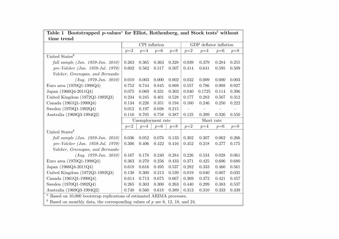
Table 1 Bootstrapped p-values for Elliot, Rothenberg, and Stock tests withouttime trend

CPI inflation GDP deflator inflation

p=2 p=4 p=6 p=8 p=2 p=4 p=6 p=8

United States

full sample (Jan. 1959-Jun. 2010) 0.263 0.365 0.363 0.328 0.039 0.379 0.284 0.255

pre-Volcker (Jan. 1959-Jul. 1979) 0.602 0.562 0.517 0.507 0.414 0.641 0.595 0.509

Volcker, Greenspan, and Bernanke

(Aug. 1979-Jun. 2010) 0.010 0.003 0.000 0.002 0.032 0.009 0.000 0.003

Euro area (1970Q1-1998Q4) 0.752 0.744 0.845 0.869 0.557 0.786 0.908 0.927

Japan (1966Q4-2011Q4) 0.075 0.069 0.331 0.303 0.040 0.1725 0.114 0.396

United Kingdom (1972Q1-1992Q3) 0.234 0.245 0.401 0.528 0.177 0.283 0.567 0.312

Canada (1961Q1-1990Q4) 0.134 0.226 0.351 0.194 0.160 0.246 0.250 0.222

Sweden (1970Q1-1992Q4) 0.012 0.197 0.038 0.215 — — — —

Australia (1969Q3-1994Q2) 0.116 0.705 0.758 0.387 0.125 0.399 0.326 0.550

Unemployment rate Short rate

p=2 p=4 p=6 p=8 p=2 p=4 p=6 p=8

United States

full sample (Jan. 1959-Jun. 2010) 0.036 0.052 0.076 0.133 0.302 0.307 0.062 0.266

pre-Volcker (Jan. 1959-Jul. 1979) 0.306 0.406 0.422 0.416 0.452 0.218 0.277 0.175

Volcker, Greenspan, and Bernanke

(Aug. 1979-Jun. 2010) 0.167 0.178 0.240 0.284 0.226 0.534 0.028 0.061

Euro area (1970Q1-1998Q4) 0.363 0.270 0.256 0.433 0.371 0.425 0.606 0.680

Japan (1966Q4-2011Q4) 0.618 0.616 0.495 0.537 0.282 0.333 0.460 0.561

United Kingdom (1972Q1-1992Q3) 0.138 0.300 0.213 0.539 0.019 0.040 0.007 0.035

Canada (1961Q1-1990Q4) 0.614 0.713 0.675 0.667 0.369 0.372 0.421 0.457

Sweden (1970Q1-1992Q4) 0.265 0.303 0.300 0.263 0.440 0.299 0.383 0.537

Australia (1969Q3-1994Q2) 0.748 0.560 0.618 0.389 0.313 0.310 0.333 0.439 Based on 10,000 bootstrap replications of estimated ARIMA processes. Based on monthly data, the corresponding values of p are 6, 12, 18, and 24.

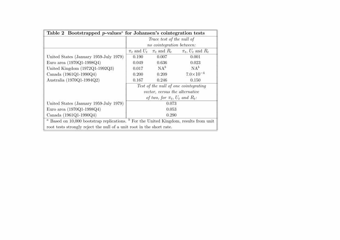
Table 2 Bootstrapped p-values for Johansen’s cointegration testsTrace test of the null of

no cointegration between:

and and , and

United States (January 1959-July 1979) 0.190 0.007 0.001

Euro area (1970Q1-1998Q4) 0.049 0.636 0.023

United Kingdom (1972Q1-1992Q3) 0.017 NA NA

Canada (1961Q1-1990Q4) 0.200 0.209 7.0×10−4Australia (1970Q1-1994Q2) 0.167 0.246 0.150

Test of the null of one cointegrating

vector, versus the alternative

of two, for , and :

United States (January 1959-July 1979) 0.073

Euro area (1970Q1-1998Q4) 0.053

Canada (1961Q1-1990Q4) 0.290 Based on 10,000 bootstrap replications. For the United Kingdom, results from unit

root tests strongly reject the null of a unit root in the short rate.

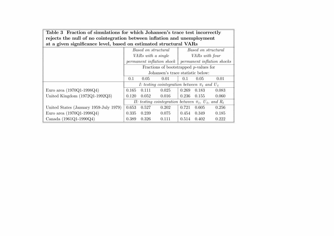
Table 3 Fraction of simulations for which Johansen’s trace test incorrectly

rejects the null of no cointegration between inflation and unemployment

at a given significance level, based on estimated structural VARs

Based on structural Based on structural

VARs with a single VARs with four

permanent inflation shock permanent inflation shocks

Fractions of bootstrapped p-values for

Johansen’s trace statistic below:

0.1 0.05 0.01 0.1 0.05 0.01

I: testing cointegration between and U

Euro area (1970Q1-1998Q4) 0.165 0.111 0.025 0.269 0.183 0.083

United Kingdom (1972Q1-1992Q3) 0.120 0.052 0.016 0.236 0.155 0.060

II: testing cointegration between , U , and R

United States (January 1959-July 1979) 0.653 0.527 0.202 0.721 0.605 0.256

Euro area (1970Q1-1998Q4) 0.335 0.239 0.075 0.454 0.349 0.185

Canada (1961Q1-1990Q4) 0.389 0.326 0.111 0.514 0.402 0.222

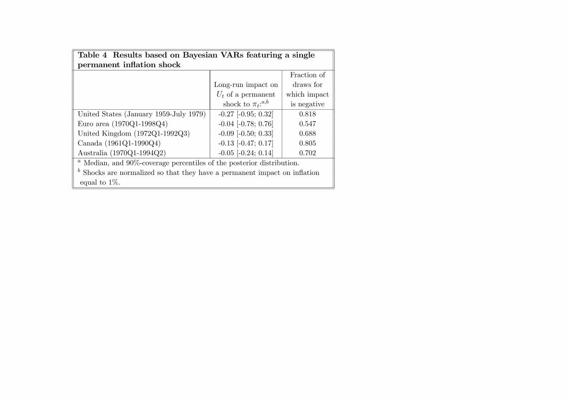
Table 4 Results based on Bayesian VARs featuring a single

permanent inflation shock

Fraction of

Long-run impact on draws for

of a permanent which impact

shock to : is negative

United States (January 1959-July 1979) -0.27 [-0.95; 0.32] 0.818

Euro area (1970Q1-1998Q4) -0.04 [-0.78; 0.76] 0.547

United Kingdom (1972Q1-1992Q3) -0.09 [-0.50; 0.33] 0.688

Canada (1961Q1-1990Q4) -0.13 [-0.47; 0.17] 0.805

Australia (1970Q1-1994Q2) -0.05 [-0.24; 0.14] 0.702 Median, and 90%-coverage percentiles of the posterior distribution. Shocks are normalized so that they have a permanent impact on inflation

equal to 1%.

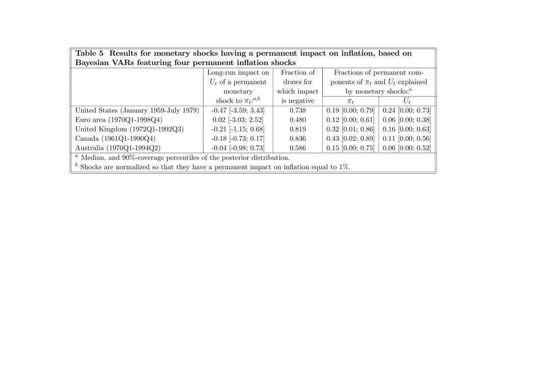
Table 5 Results for monetary shocks having a permanent impact on inflation, based on

Bayesian VARs featuring four permanent inflation shocks

Long-run impact on Fraction of Fractions of permanent com-

of a permanent draws for ponents of and explained

monetary which impact by monetary shocks:

shock to : is negative

United States (January 1959-July 1979) -0.47 [-3.59; 3.43] 0.738 0.19 [0.00; 0.79] 0.24 [0.00; 0.73]

Euro area (1970Q1-1998Q4) 0.02 [-3.03; 2.52] 0.480 0.12 [0.00; 0.61] 0.06 [0.00; 0.38]

United Kingdom (1972Q1-1992Q3) -0.21 [-1.15; 0.68] 0.819 0.32 [0.01; 0.86] 0.16 [0.00; 0.63]

Canada (1961Q1-1990Q4) -0.18 [-0.73; 0.17] 0.836 0.43 [0.02; 0.89] 0.11 [0.00; 0.56]

Australia (1970Q1-1994Q2) -0.04 [-0.98; 0.73] 0.586 0.15 [0.00; 0.75] 0.06 [0.00; 0.52] Median, and 90%-coverage percentiles of the posterior distribution. Shocks are normalized so that they have a permanent impact on inflation equal to 1%.

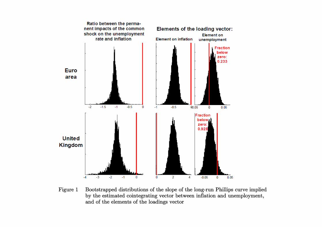
22

Figure 1 Bootstrapped distributions of the slope of the long-run Phillips curve implied

by the estimated cointegrating vector between inflation and unemployment, and of the elements of the loadings vector

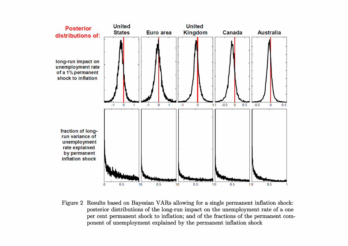
23

Figure 2 Results based on Bayesian VARs allowing for a single permanent inflation shock: posterior distributions of the long-run impact on the unemployment rate of a one per cent permanent shock to inflation; and of the fractions of the permanent com- ponent of unemployment explained by the permanent inflation shock

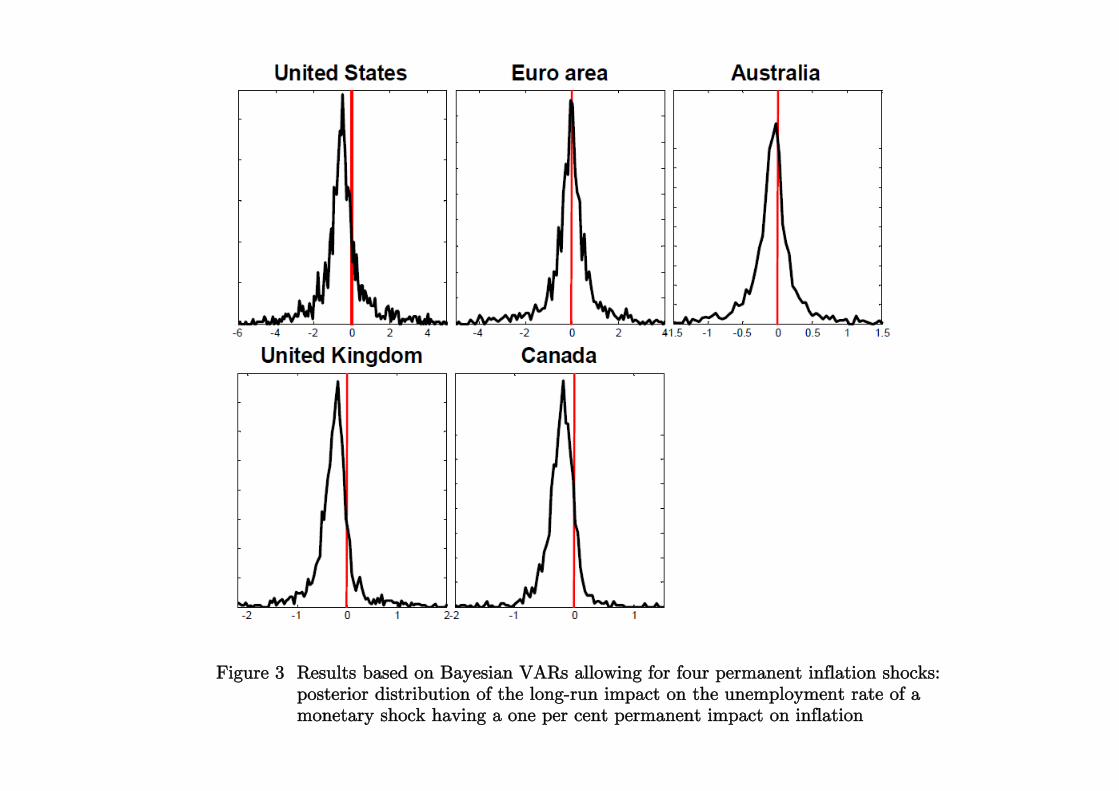
24

Figure 3 Results based on Bayesian VARs allowing for four permanent inflation shocks: posterior distribution of the long-run impact on the unemployment rate of a monetary shock having a one per cent permanent impact on inflation

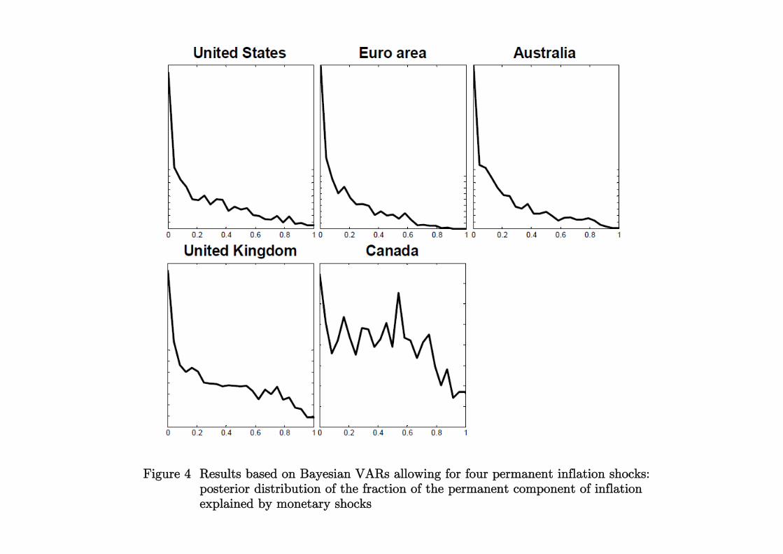
25

Figure 4 Results based on Bayesian VARs allowing for four permanent inflation shocks: posterior distribution of the fraction of the permanent component of inflation explained by monetary shocks

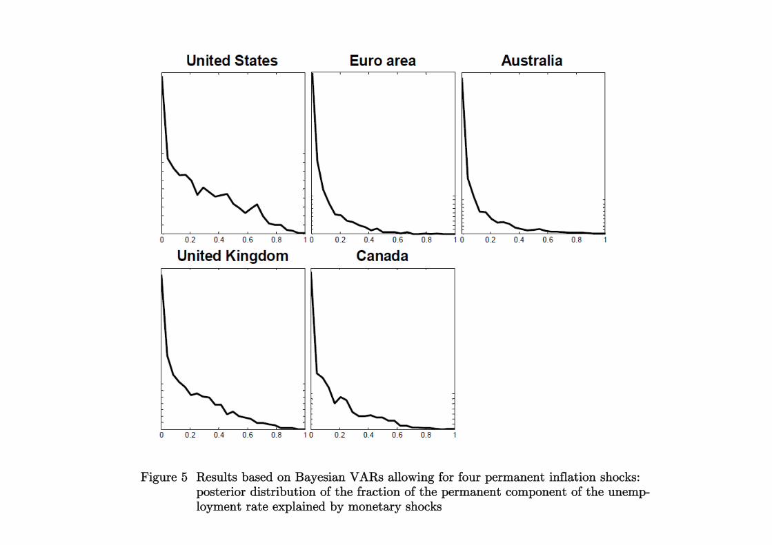
26

Figure 5 Results based on Bayesian VARs allowing for four permanent inflation shocks: posterior distribution of the fraction of the permanent component of the unemp- loyment rate explained by monetary shocks