The landward and seaward mechanisms of fine-sediment transport across intertidal flats in the...

Continental Shelf Research 60S (2013) S85–S98

Contents lists available at SciVerse ScienceDirect

Continental Shelf Research

0278-43

doi:10.1

n Corr

E-m1 N

Taiwan.

journal homepage: www.elsevier.com/locate/csr

Research papers

The landward and seaward mechanisms of fine-sediment transport acrossintertidal flats in the shallow-water region—A numerical investigation

Tian-Jian Hsu a,n, Shih-Nan Chen b,1, Andrea S. Ogston c

a Center for Applied Coastal Research, Civil and Environmental Engineering, University of Delaware, Newark, DE 19716, USAb Applied Ocean Physics and Engineering, Woods Hole Oceanographic Institution, Woods Hole, MA 02543, USAc School of Oceanography, University of Washington, Seattle, WA 98195, USA

a r t i c l e i n f o

Article history:

Received 18 March 2011

Received in revised form

30 January 2012

Accepted 8 February 2012Available online 23 February 2012

Keywords:

Tidal flats

Sediment transport

Settling lag

Numerical modeling

43/$ - see front matter & 2012 Elsevier Ltd. A

016/j.csr.2012.02.003

esponding author.

ail address: [email protected] (T.-J. Hsu).

ow at Institute of Oceanography, National

a b s t r a c t

This study investigates transport of fine sediment across idealized intertidal flats with emphasis on

resolving processes at the tidal edge, which is defined as the very shallow region of the land–water

interface. We first utilize a two-dimensional, vertical numerical model solving the non-hydrostatic

Reynolds-averaged Navier–Stokes equations with a k–e turbulence closure. The numerical model

adopts the Volume of Fluid method to simulate the wetting and drying region of the intertidal flat. The

model is demonstrated to be able to reproduce the classic theory of tidal-flat hydrodynamics of

Friedrichs and Aubrey (1996) and to predict the turbidity at the tidal edge that is similar, qualitatively,

to prior field observations. The Regional Ocean Modeling System (ROMS) is also utilized to simulate the

same idealized tidal flat to evaluate its applicability in this environment. We demonstrate that when a

small critical depth (hcrit¼2 cm) in the wetting and drying scheme is adopted, ROMS is able to predict

the main features of hydrodynamics and sediment-transport processes similar to those predicted by

the RANS–VOF model. When driving the models with a symmetric tidal forcing, both models predict

landward transport on the lower and upper flat and seaward transport in the subtidal region. When the

very shallow region of the tidal edge is well resolved, both models predict an asymmetry of tidal

velocity magnitude between the flood and the ebb that may encourage landward sediment transport on

the flat. Further model simulation suggests that the predicted landward transport of sediment on the

flat is mainly due to the settling-lag effect while the asymmetry of tidal velocity magnitude may add a

lesser but non-negligible amount. When the bed erosion is limited by the availability of soft mud, the

predicted transport direction becomes landward in both the subtidal region and on the flat. These

results suggest that the tidal flow generally encourages landward transport while significant seaward

transport may be caused by other mechanisms. Comparisons with field observations show similarities

in the net landward transport on the flat and enhanced stresses and suspended-sediment concentra-

tions near the very shallow region of the tidal edge. The field results also indicate significant transport

of sediment occurs through the channels, as a function of three-dimensional processes, which are not

incorporated in the present idealized modeling.

& 2012 Elsevier Ltd. All rights reserved.

1. Introduction

Intertidal flats create the critical linkage between the deeperpart of the estuary (e.g., tidal channels) and the vegetated upperflat, e.g., salt marshes. The morphology of many tidal flats is invery subtle dynamic equilibrium (de Swart and Zimmerman,2009; see Le Hir et al., 2000, for a review) and hence they arealso very vulnerable to natural and anthropogenic influences.

ll rights reserved.

Taiwan University, Taipei,

To preserve or even to reclaim intertidal habitat, it is critical tounderstand various mechanisms causing landward and seawardtransport. This requires development of numerical modeling toolsfor predicting and managing the shallow estuarine ecosystem.

The classic equilibrium theory of intertidal flat morphologydeveloped by Friedrichs and Aubrey (1996) (subsequently referredto as FA96) is based on pure kinematic analysis (mass conservation).According to FA96, the maximum tidal velocity magnitude U in thesubtidal and the lower flat regions is calculated by

U ¼LpT

, xrL=2 ð1aÞ

where L is the horizontal distance from the low to high water line andT is the tidal period (see also Fig. 1). At the upper flat, maximum tidal

www.elsevier.com/locate/csr

www.elsevier.com/locate/csr

dx.doi.org/10.1016/j.csr.2012.02.003

http://crossmark.dyndns.org/dialog/?doi=10.1016/j.csr.2012.02.003&domain=pdf



mailto:[email protected]

dx.doi.org/10.1016/j.csr.2012.02.003

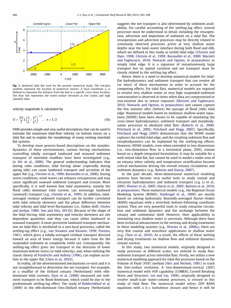
Fig. 1. Idealized tidal flat used for the present numerical study. The red-plus

symbols represent the location of numerical sensors. A local coordinate zb is

defined to represent the distance from the bed at a specific cross-shore location.

The blue line represents the water-surface elevation at low (solid) and high

(dashed) tides.

T.-J. Hsu et al. / Continental Shelf Research 60S (2013) S85–S98S86

velocity magnitude is calculated by

U ¼2pT

Lx

L�

x2

L2

� �1=2

, x4L=2 ð1bÞ

FA96 provides simple and very useful descriptions that can be used toestimate the maximum tidal-flow velocity (or bottom stress) on atidal flat and to explain the morphology of many existing intertidalflat systems.

To develop more process-based descriptions on the morpho-dynamics of these environments, various forcing mechanismscontrolling tidally averaged landward and seaward sedimenttransport of intertidal mudflats have been investigated (e.g.,Le Hir et al., 2000). The general understanding indicates thatduring calm conditions, tidal forcing alone (especially duringspring tide) can cause landward transport and accretion of theupper flat (e.g., Christie et al., 1999; Bassoullet et al., 2000). Duringstorm conditions, wind waves can enhance resuspension and maycause significant seaward sediment transport and erosion. Morespecifically, it is well known that tidal asymmetry, namely theflood (ebb) dominant tidal current, can encourage landward(seaward) transport (e.g., Christie et al., 1999). In addition, tidal-averaged residual sediment transport can be further correlatedwith tidal velocity skewness and the phase difference betweentidal velocity and tidal level fluctuations (i.e., Stokes drift; Unclesand Jordan, 1980; Son and Hsu, 2011b). Because of the shape ofthe tidal forcing, tidal asymmetry and velocity skewness are sitedependent quantities and they can cause either landward orseaward transport. A more persistent landward transport mechan-ism on tidal flats is attributed to a non-local processes, called thesettling-lag effect (e.g., van Straaten and Keunen, 1958; Postma,1961), which gives a tidally-averaged residual transport directedtoward an area of lower energy because it takes time for thesuspended sediment to completely settle out. Consequently, thesettling-lag effect gives net transport in the direction of lowermaximum bottom stress (or tidal velocity), and, when utilizing theclassic theory of Friedrichs and Aubrey (1996), can explain accre-tion in the upper flat (Chen et al., 2010).

In reality, all the aforementioned mechanisms co-exist and it isnot straightforward to determine the net transport. For example,at a mudflat of the Dollard estuary (Netherland) with ebb-dominant tidal currents, Dyer et al. (2000) measured net sedi-ment transport to be flood-dominant, which could be due to thepredominant settling-lag effect. The study of Ridderinkhof et al.(2000) in the ebb-dominant Ems-Dollard estuary (Netherland)

suggests the net transport is also determined by sediment avail-ability. For careful accounting of the settling-lag effect, severalprocesses must be understood in detail, including the resuspen-sion, advection and deposition of sediment on a tidal flat. Theresuspension and advection processes may be directly related tocommonly observed processes active at very shallow waterdepths near the land–water interface during both flood and ebb,which we defined in this study as turbid tidal edge (Christie andDyer, 1998; Christie et al., 1999; Bassoullet et al., 2000; Mariottiand Fagherazzi, 2010; Nowacki and Ogston, in preparation) orsimply tidal edge. It is a signature of instantaneously largetransport but its spatial variation and net transport must beclosely related to the settling-lag effect.

Hence, there is a need to develop numerical models for tidal-flat hydrodynamics and sediment transport that can resolve all(or most) of these mechanisms in order to account for thecompeting effects. For tidal flats, numerical models are requiredto resolve very shallow water as very high suspended-sedimentconcentration is observed at times when data are compromised ornon-existent due to sensor exposure (Mariotti and Fagherazzi,2010; Nowacki and Ogston, in preparation) and cannot capturethe few minutes after (before) the passage of flood (ebb) tidaledge. Numerical models based on nonlinear shallow-water equa-tions (NSWE) have been shown to be capable of simulating thecross-shore hydrodynamics, sediment transport and morphody-namic processes in idealized tidal flats (Roberts et al., 2000;Pritchard et al., 2002; Pritchard and Hogg, 2003). Specifically,Pritchard and Hogg (2003) demonstrate that the NSWE modelcaptures the turbid tidal edge, and the resulting sediment flux andmorphodynamics can be explained by the settling-lag effects.However, NSWE models, even when extended to two dimensions(i.e., two-dimension flow in a horizontal plane, 2DH), remainbased on a depth-integrated formulation. It may be suitable for awell-mixed tidal flat, but cannot be used to model a wider area ofan estuary when salinity and temperature stratification becomecritical mechanisms driving the overall estuary circulations andsediment dynamics (e.g., Ralston and Stacey, 2007).

In the past decade, three-dimensional numerical modelingsystems have become very useful tools to study coastal andestuarine hydrodynamics and sediment transport (e.g. Li et al.,2005; Warner et al., 2005; Harris et al., 2005; Ralston et al., 2010,in preparation). These numerical models (e.g., the Regional OceanModeling System (ROMS), Haidvogel et al., 2000) are mostlybased on solving hydrostatic Reynolds-averaged Navier–Stokes(RANS) equations with a stretched, bottom-following coordinatesystem. They are very powerful tools to study estuarine circula-tion and sediment dynamics and the exchange between theestuary and continental shelf. However, their applicability insimulating very shallow water is uncertain. Although there havebeen technical advancement in the wetting and drying treatmentsin these modeling systems (e.g., Warner et al., 2008a), there arevery few coastal and nearshore applications in shallow water(e.g., Chen et al., 2010). As a result, the effects of these wettingand drying treatments on shallow flow and sediment dynamicsremain unclear.

In this study, two numerical models, originally designed tostudy processes at different scales, are utilized to study fine-sediment transport across intertidal flats. Firstly, we utilize a newnumerical modeling approach for tidal-flat processes based on theVolume of Fluid (VOF) method (Hirt and Nichols, 1981) to trackthe free-surface evolution. A two-dimensional-vertical (2DV)numerical model with VOF capability (COBRAS, Cornell BreakingWave and Structure; Lin and Liu, 1998), originally designed toresolve small-scale water-column processes, is revised in thisstudy of tidal flow. The numerical model solves 2DV RANSequations with a k–e turbulence closure and hence it will be

T.-J. Hsu et al. / Continental Shelf Research 60S (2013) S85–S98 S87

called the RANS–VOF model in this paper. To understand thecapability of a large-scale coastal modeling system in simulatinglarge amounts of landward and seaward transport across theintertidal flats, ROMS is also utilized. Inter-comparisons of modelresults between RANS–VOF and ROMS for fine sediment transportacross idealized intertidal flats are reported.

The RANS–VOF model is used to simulate processes of hydro-dynamics and sediment transport across an idealized tidal flat withflow conditions similar to Willapa Bay (Nittrouer et al., 2013). High-resolution numerical model results are then used to investigateprocesses that occur at the turbid tidal edge. In particular, we studylandward and seaward sediment fluxes and the relationship betweenthe upper intertidal region and the lower completely submergedregion. Because the VOF model is computationally expensive and canonly be used in idealized conditions, the second objective is to carryout inter-comparisons between the results of RANS–VOF and ROMS.We evaluate the capability of ROMS in simulating hydrodynamicsand sediment transport in tidal flats by changing the critical depth ofthe wetting and drying scheme. Finally, field data of flow velocity andsuspended-sediment-concentration profiles measured in a channel-flat system are presented in order to appreciate the complexity in thefield condition and to test several qualitative features obtained in theidealized numerical study.

2. Numerical models

2.1. RANS–VOF model

A 2DV-RANS model for sediment-laden flow with a k–eturbulence closure is utilized here to study cross-shore finesediment transport in intertidal flats. This numerical model isan extension of the wave model, COBRAS (Lin and Liu, 1998)utilized to study various surf-zone wave problems (e.g., Lin andLiu, 1998; Lara et al., 2006). The backbone of the COBRAS model isa two-dimensional Navier–Stokes solver with a Volume of Fluid(VOF) scheme for free surface tracking called RIPPLE, developedoriginally by Los Alamos National Laboratory (Kothe et al., 1991).This numerical model has recently been extended with a finesediment-transport capability in order to study wave–mud inter-actions (Torres-Freyermuth and Hsu, 2010). In the present study,we revised the code used in Torres-Freyermuth and Hsu (2010)for tidal flow applications. In the dilute limit, which is the casehere, the sediment transport formulation adopted in RANS–VOF issimilar to that of ROMS where sediment concentration is calcu-lated by mass conservation and sediment-induced density candrive gravity flow and cause damping of carrier flow turbulence.

2.1.1. Model formulation

The present model adopts the assumption of fine-grained sedimentand hence the complete two-phase flow formulation for particle-ladenflow can be significantly simplified (Balachandar and Eaton, 2010;Torres-Freyermuth and Hsu, 2010). The rigorous justification of thisfine sediment approximation requires the particle response time (seeEq. (3)) to be smaller than the Kolmogorov timescale. Particle responsetime is a measure of the timescale required for a single particle tofollow the ambient fluid flow (Balachandar and Eaton, 2010). A simpleexample is demonstrated here to support our assumption. Weconsider fine-grained sediment transport in an intertidal mudflatwhere the settling velocity is no more than O(1) mm/s. The settlingvelocity can be calculated by Stokes law:

Ws ¼ðrs�rÞgd2

18mð2Þ

where r is the fluid density, m is the fluid viscosity, and g is thegravitational acceleration. If we consider silt transported as primary

particles with grain size d¼34 mm and sediment density rs¼

2650 kg/m3, the settling velocity is calculated to be 1 mm/s and thecorresponding particle response time

Tp ¼Ws

ð1�r=rsÞgð3Þ

is only 1.6�10�4 s. Considering a typical turbulent dissipation rate ina meso-tidal environment of e¼O(10�4–10�3) (Fettweis et al., 2006),the Kolmogorov timescale is only 0.03–0.1 s, which is about twoorders of magnitude larger than the particle response time. Similarly, ifwe consider a flocculated particle of size d¼60 mm and floc densityrs¼1250 kg/m3 (using a fractal dimension 2.3 and primary particle

size of 4 mm; Kranenburg, 1994), the resulting settling velocity is0.5 mm/s and the particle response time is only Tp¼2.6�10�4 s. Insummary, for a typical intertidal flat, fine sediments are almost passiveto the carrier flow other than the effects of settling velocity. Hence,sediment transport can be calculated by mass conservation and theonly effect of sediment on the carrier flow that needs to be consideredis the sediment-induced density stratification (Ozdemir et al., 2010).

The numerical model is based on Reynolds-averaged two-dimensional-vertical formulation for fluid flow and suspended-sediment transport. The continuity equation is written as

@ð1�fÞ@t

þ@ð1�fÞu

@xþ@ð1�fÞw

@z¼ 0 ð4Þ

where f is the sediment volumetric concentration, u is the flowvelocity in the x- (streamwise or cross-shore) direction and w isthe velocity in the z- (vertical) direction. The flow momentumequations in the streamwise and vertical directions are written as

@u

@tþu

@u

@xþw

@u

@z¼�

1

r@p

@xþ

1

rð1�fÞ@tf

xz

@zþ@tf

xx

@x

!ð5Þ

and

@w

@tþu

@w

@xþw

@w

@z¼�

1

r@p

@zþ

1

rð1�fÞ@tf

zz

@zþ@tf

zx

@x

!� 1þ

ðs�1Þfð1�fÞ

� �g

ð6Þ

where p is the fluid pressure, s¼rs/r is the specific gravity and tf

represents the fluid stresses, including viscous and turbulentstresses. The last term on the right-hand-side of Eq. (6) representsthe sediment-induced buoyancy effect. Sediment concentration iscalculated by mass balance:

@f@tþ@fu

@xþ@fw

@z¼@fWs

@zþ@

@z

nt

scþDc

� �@f@z

� �þ@

@x

nt

scþDc

� �@f@x

� �ð7Þ

where vt is the eddy viscosity, sc is the Schmidt number and Dc isthe viscous (Brownian) diffusion coefficient. Settling velocity Ws

is calculated by Eq. (2). Hindered settling effects are not impor-tant in this study because the maximum sediment concentrationcalculated is no more than 15 g/L (volumetric concentration 0.6%).

Closure of turbulent Reynolds stress is based on the eddyviscosity hypothesis:

tfij ¼ rðnþntÞ

@ui

@xjþ@uj

@xi

� ��

2

3rð1�fÞkdij�

2

3rnt

@ul

@xldij ð8Þ

where i, j¼1, 2 for 2DV flow and dij is the Kronecker delta. Theeddy viscosity is further calculated by the k–e closure

nt ¼ Cmk2ð1�fÞe ð9Þ

where k is the turbulent kinetic energy (TKE), e is the turbulentdissipation rate and Cm is an empirical coefficient. The balance


equations for k and e are written as

ð1�fÞ@k

@tþ@kuj

@xj

� �¼tf

ij

r@ui

@xjþ

@

@xjnþ nt

sk

� �@ð1�fÞk@xj

� ��ð1�fÞe

þgnt

scðs�1Þ

@f@z

ð10Þ

and

ð1�fÞ@e@tþ@euj

@xj

� �¼ Ce1

ek

tfij

r@ui

@xjþ

@

@xjnþ nt

se

� �@ð1�fÞe@xj

� �

�ð1�fÞCe2e2

kþCn

e3ek

gnt

scðs�1Þ

@f@z

ð11Þ

These two equations are essentially the standard k–e equationsfor particle-laden flow with small particle response time. Thestandard k–e equations are developed with the main assumptionsfollowing Kolmogorov hypothesis for fully turbulent flow. The lastterms of these two equations represent the effect of sediment-induced density stratification on carrier turbulent flow, which isalso a well-known mechanism for salt- or heat-stratified flow. Ifthe Boussinesq approximation for dilute sediment flow (which isthe case in this study) and the hydrostatic pressure approxima-tion are adopted, the present governing equations and closuresbecome similar to that typically used for coastal and estuarymodeling, such as ROMS.

A continuous erosion/deposition approach is utilized as thebottom boundary condition for sediment concentration. Sedimenterosion flux from the bottom is specified by the followingformula:

E¼ btbðtÞ

tc�1

� �ð12Þ

where b (m/s) is an empirical erosion flux coefficient and tbðtÞ isthe bottom stress. In this study, a constant critical shear stress forerosion is adopted in most cases for simplicity. The logarithmiclaw for a rough bed is applied between the bed and the first halfgrid point above the bed to estimate bottom stress. The resultingbottom stress is further used as bottom boundary condition forthe streamwise flow velocity (u) and to estimate the boundarycondition for turbulent kinetic energy (k), turbulent dissipationrate (e), and sediment erosion flux. More details on the bottomboundary conditions for boundary layer and sediment transportcan be found in Torres-Freyermuth and Hsu (2010).

2.1.2. Numerical implementation

The 2DV-RANS–VOF model is based on a finite differencescheme, which is second-order accurate in spatial discretization.The mass and momentum equations are solved by the two-stepproject method, a solution technique commonly used for incom-pressible Navier–Stokes equations. The fully explicit two-stepproject scheme is utilized in this study to save computationaltime and hence the temporal discretization is only first-orderaccurate. A central difference scheme is used for various diffusionterms in the governing equations and a combined upwind andcentral difference scheme is used for advection/convection terms.The time-step size is determined every computational cycle basedon the Courant–Friedrichs–Lewy condition and the maximumtime step is set to be no more than 0.05 s.

The present model adopts a VOF variable, F(x,z,t), to describethe free surface (Hirt and Nichols, 1981). For a grid cell comple-tely occupied by water, F is defined to be 1.0. On the other hand,for a grid cell completely occupied by air, F¼0. For an interfacecell that is partly occupied by water and partly occupied by air,F represents the fraction of the volume occupied by water, i.e.,0oFo1. At every time step, the F value is updated by an

advection equation of F(x,z,t):

@F

@tþu

@F

@xþw

@F

@z¼ 0 ð13Þ

The time-dependent free-surface location can be reconstructedfrom F. For any free-surface flow, Eq. (13) essentially representsthe kinematic boundary condition of the flow. The VOF scheme isoriginally developed to resolve effectively the detailed interfacedynamics of two phase flow (e.g., air and water). Because theF value within a grid point follows the mass balance via Eq. (13),the VOF scheme can describe free-surface flow within one gridpoint (in a grid-averaged sense). In this study, numerical experi-ments further suggest when the volume of fluid value in a gridcell is below about 0.3 and the cell is directly above the solidbottom, the advection of fluid to the adjacent cell can cause noisein velocity due to numerical approximation. This numericalfluctuation may be minimized with a smaller time step or gridsize. A cut-off value for the minimum F to be calculated in thenumerical scheme is set to be Fmin¼0.01. A larger cut-off value ofthe VOF function can also be used to minimize the noise. Moredetails of using volume of fluid approach for free-surface flow canbe found in Hirt and Nichols (1981). The accuracy of the presentnumerical model, and particularly the VOF scheme in simulatingshallow water process has been demonstrated in many priorstudies, such as those describing swash zone processes (Lara et al.,2006), dam break waves (Shigematsu et al., 2004) and borepropagation over a slope (Zhang and Liu, 2008). The readersare referred to these earlier studies for more detailed modelvalidations.

The numerical model utilizes a partial-cell treatment (Kotheet al., 1991) for solid obstacles in the computational domain.Although the partial-cell treatment provides a robust scheme toapproximate solid boundaries of arbitrary shape, the numericalaccuracy near the solid boundary is low, which is not appropriatefor the present application where tidal bottom-boundary-layerprocesses need to be well-resolved. Hence, the computationaldomain is rotated with an angle equal to the slope of the flat sothat the bed surface can be accurately resolved with a rectanglemesh system. The no-flux boundary condition and zero-gradientboundary condition are applied for the flow velocity, k, e andsediment concentration at the free-surface. A zero value of fluidpressure is applied at free-surface. For the rest of the boundaries,the gradient of pressure is specified to be zero.

To improve the accuracy of the lower order scheme used in theRANS–VOF model, we use fine spatial resolution and a small timestep. We carried out a grid refinement test and found that theresolution adopted here is appropriate to evaluate the tidallyaveraged sediment-transport rate. For the present vertical gridsize (Dz¼0.05 m, see Section 3.1), the numerical diffusion (ornumerical viscosity¼10�5–10�4 m2/s) is at least one order ofmagnitude smaller than the eddy viscosity (O(10�3) m2/s). Hence,the present low-order numerical scheme is appropriate forRANS modeling where mixing is dominated by eddy viscosity/diffusivity.

2.2. Regional ocean modeling system (ROMS)

As we will demonstrate next, the RANS–VOF simulations arecomputationally expensive. Due to this limitation, the RANS–VOFcannot be easily applied to realistic coastal problems with spatialscales over tens of kilometers. Hence, one of the main objectivesof this study is to conduct inter-comparisons between RANS–VOFand ROMS models, and to evaluate the capability of ROMS,specifically the wetting and drying scheme, in simulatingprocesses across the shallow-water region of the tidal flats.

Table 1


ROMS is a three-dimensional, hydrostatic, primitive-equationocean model that solves the Reynolds-averaged form of theNavier–Stokes equations on a horizontal orthogonal curvilinearArakawa ‘‘C’’ grid and uses stretched bottom-following coordi-nates in the vertical direction. The model formulation, numericalschemes, and the implementations of turbulence closures andboundary conditions are described in Haidvogel et al. (2000),Shchepetkin and McWilliams (2005), Warner et al. (2005), andMarchesiello et al. (2001). ROMS incorporates a suspended-sedi-ment transport module that has been validated against laboratoryexperiments (e.g., Warner et al., 2008a). Suspended sediment isincorporated in the fluid density calculation and hence sediment-induced density stratification can damp the flow turbulence inthe two-equation turbulence closure. ROMS with the sedimentmodule has been applied to a wide range of idealized and realisticcoastal flow problems (e.g., Chen et al., 2009, 2010; Warner et al.,2008b) and has been demonstrated to have high skill in thesimulation of observed salinity, velocity and turbulence (Warneret al., 2005; Li et al., 2005; Hetland and MacDonald, 2008).Moreover, the numerical model is parallelized. Thus, computa-tionally intensive modeling work can be completed efficiently.

For tidal-flat applications, we need to utilize the existingwetting and drying scheme in ROMS to model the region of veryshallow flow depth (Warner et al., 2008a). In this numericaltreatment, a critical depth hcrit is specified. When the water depthof a computation cell is smaller than hcrit, the cell is considered‘‘dry’’ and the fluxes to the adjacent cells are blocked (Casulli andCheng, 1992). Most prior studies specify a rather large hcrit to savecomputational time and to ensure the shallow water region of thedomain does not affect the inner flow field of interest. In thisstudy, ROMS is utilized to carry out an idealized cross-shore studyon an intertidal flat and variable hcrit are specified.

There are several main differences between the RANS–VOFmodel and ROMS. Firstly, in the RANS–VOF model, the full RANSequations are solved without hydrostatic approximations. Thepresent geometry has a very mild slope and hence the non-hydrostatic pressure effect may be of minor significance. Theimportance of the non-hydrostatic effect will be investigatedlater. Secondly, the Boussinesq approximation is adopted forsediment-induced buoyancy effects in ROMS. For the presentstudy, sediment concentration is dilute and hence the effect ofthe Boussinesq approximation is negligible. Therefore, it isexpected that the major difference between ROMS and RANS–VOF is due to the numerical treatment of the wetting and dryingscheme in very shallow water. As discussed in Section 2.1.2, theVOF scheme is able to calculate shallow flow depth of aboutO(1) cm (in a grid-averaged sense) when a Dz¼5 cm is used. Onthe other hand, the minimum depth that can be resolved byROMS is directly determined by hcrit. Our model comparisondemonstrates that when a very small hcrit¼2 cm is used, ROMSmodel results are similar to those simulated by RANS–VOF. Inaddition, the computational time required by ROMS at this smallhcrit value is significantly smaller than that of RANS–VOF.

Summary of all model runs investigated in this study.

Case

no.

Settling velocity,

Ws (mm/s)

Crit. stress,

tb (Pa)

Additional comments

1 0.5 0.15

2 0.5 0.15 Case 1 without

sediment-induced

density stratification

3 0.25 0.15 Lower settling velocity

4 1.0 0.15 Higher settling velocity

5 0.5 0.13 Lower critical shear

stress

6 0.5 0.15 Case 1 but with limited

erosion

3. Cross-shore transport on an idealized intertidal flat

3.1. Geometry

In this study, we investigate cross-shore transport of finesediment on intertidal flats using the RANS–VOF numerical modeland ROMS. A schematic plot of the numerical model domain setupis illustrated in Fig. 1. The idealized tidal flat has a constant slopeof a and the initial (low tide) water level is set to be 3.5 m forall the runs. The initial water line intercepts with the flat atx¼0 m at low water and the flow is driven by a prescribed

sinusoidal tidal-level variation of tidal amplitude Z (m) and tidalperiod of T¼12 h. Hence, the region of xo0 m is completelysubmerged during the tidal passage and is defined as the subtidalregion. The horizontal distance from the low to high water line isL¼Z/a. The lower flat is defined here as the region between x¼0and x¼L/2 and the upper flat is defined as the region betweenx¼L/2 and x¼L. The hydrodynamics and sediment-transportprocesses that occur in these three regions, namely the subtidalregion, the lower-flat region and the upper-flat region, are quitedistinct and hence differentiating between them is a main focus ofour numerical investigation.

Numerical runs focus on an idealized Willapa Bay where thetidal-flat slope is set to be a¼0.0013 and the tidal range is set tobe Z¼4.25 m. For RANS–VOF simulations, the grid size in thestreamwise direction (x) and vertical direction (z) is set to beDx¼10 m and Dz¼0.05 m, respectively. Grid refinement testsindicate that simulations with half the grid size only change theresulting sediment concentration by 10%. Hence, the main flowfeatures have low sensitivity to further grid refinement. For thisset of grid resolution, the time step is typically around 0.01 s. Inthe main numerical run (Case 1 in Table 1), the settling velocity isset to a constant of Ws¼0.5 mm/s and the critical shear stress isalso set to a constant of tc¼0.15 Pa (Hill et al., in preparation;Wiberg et al., in preparation). The bottom roughness in thenumerical simulation is set to be Ks¼2.4 cm (z0¼0.8 mm), whichis commonly used in other numerical studies of tidal flat toconsider small scale bedforms and runnels (e.g., Le Hir et al.,2000). Additional runs with different settling velocity and bederodibility are also carried out in order to investigate the effect ofthese parameters in the resulting cross-shore sediment transport.A summary of all the model runs is given in Table 1.

Case 1 is further simulated by ROMS using different hcrit valuesin the wetting and drying scheme (hcrit¼10, 5, 2 cm). Modelresults suggest that ROMS can capture the main characteristicspredicted by RANS–VOF (see Section 3.3), when a smallhcrit¼2 cm is used (10 sigma layers in the vertical direction). Athcrit¼2 cm, the barotropic time step is 0.05 s, which is larger thanthat used in RANS–VOF. Moreover, RANS–VOF requires a muchsmaller streamwise grid size of Dx¼10 m due to the VOFscheme (as compared to Dx¼100 m in ROMS). For a 3-day modeltime using 16 processors, ROMS requires 5 h to complete thesimulation, which is about 10–15 times faster than that of RANS–VOF. It is noted here that the most time-consuming computa-tional task in RANS–VOF is to solve the non-hydrostatic pressurefield. By examining the calculated pressure field by RANS–VOF,the hydrostatic pressure distribution in the present problem is agood approximation except very near to the tidal edge. Due to thehigh computational cost, the RANS–VOF model is run for onlythree tidal cycles and the results shown here are for the third tidalcycle unless otherwise noted. Our analysis suggests resultsobtained for the third tidal cycle are similar to those of the


second cycle. For all the cases shown in this study, the tidal-averaged sediment-transport rate of the third cycle is within 5%difference from that of the second tidal cycle. More noticeabledifferences can be observed for cases of smaller settling velocity.

Fig. 3. (a) A snapshot of the velocity field and suspended-sediment concentration

during ebb (at t¼9.6 h of the third tidal cycle) for Case 1 calculated using the

RANS–VOF model. (b) Cross-shore distribution of streamwise velocity at the first

grid point (2.5 cm) above the bed (blue-dashed curve) and depth-averaged

sediment concentration (red-solid curve). This instant is chosen as the time when

the ebb tidal edge passes the same location as that shown for flood tidal edge in

Fig. 1.

3.2. Model results

3.2.1. RANS–VOF results

The hydrodynamics and suspended-sediment concentrationresults for Case 1 are presented as snapshots during floodand ebb (see Figs. 2 and 3). The numerical model predicts theturbid tidal edge during flood and ebb similar to prior studies(Christie and Dyer, 1998; Christie et al., 1999). The cross-shoredistributions of the near-bed velocity (Figs. 2b and 3b) suggest thevelocity magnitudes are more or less uniform in the lower flat butincrease significantly approaching the tidal water’s edge. Theincreased velocity magnitude is also correlated with an increasein sediment concentration. Small fluctuations in velocity near thetidal edge are numerical noise discussed in Section 2.1.1. Duringflood, the near-bed velocity increases by about 95% approachingthe tidal edge (see Fig. 2b). Near-bed velocity is directly related tobottom stress and hence the increased near-bed velocity inducesa significant amount of sediment resuspension. In this case, thesediment concentration at flood tidal edge is as large as 15 g/L.During ebb (Fig. 3b), the near-bed velocity increases (in magni-tude) by about 75% as the tidal edge is approached, which is alesser increase than that during flood. The maximum sedimentconcentration in the ebb tidal edge is about 11 g/L, generallyconsistent with observations at slightly greater water depths of43 g/L during winter ebb tides in Willapa Bay (Boldt et al., inpreparation). The observed asymmetry between flood and ebb inthe near-bed tidal velocity and suspended-sediment concentra-tion, subject to a completely symmetric tidal forcing, may causenon-zero tidally averaged sediment transport (see Section 3.3.3).

Model results are compared with the analytical theory of FA96(see Eqs. (1a) and (1b)) for the cross-shore distribution ofmaximum tidal velocity over the entire tidal cycle. For Case 1,L¼Z/a¼3270 m and hence U¼23.8 cm/s. Model results of

Fig. 2. (a) A snapshot of the velocity field and suspended-sediment concentration

during flood (at t¼2.5 h of the third tidal cycle) for Case 1 calculated using the

RANS–VOF model. (b) The corresponding cross-shore distribution of streamwise

velocity at the first grid point (2.5 cm) above the bed (blue-dashed curve) and

depth-averaged sediment concentration (red-solid curve).

Fig. 4. RANS–VOF model results showing the cross-shore distribution of depth-

averaged flow velocity throughout the tidal cycle (every 20 min, or T/36 interval,

black lines) for Case 1. The envelope of the numerical model results can be

compared with maximum tidal velocity magnitude predicted by FA96 theory (red-

dashed curves).

depth-averaged cross-shore distribution of streamwise velocitiesover the entire tidal cycle (every 20 min interval) are plotted inFig. 4 (black curves) along with theoretical maximum values, i.e.,Eqs. (1a) and (1b) suggested by FA96. The numerical modelpredicts the maximum cross-shore velocity distribution (see theenvelope of the black curves) that is consistent with FA96 for bothflood and ebb conditions. The landward reduction in the max-imum cross-shore velocity is anticipated to drive net landwardsediment transport through the settling-lag effect (e.g., vanStraaten and Keunen, 1958; Postma, 1961).

For xrL/2, numerical model results agree very well with FA96.For x4L/2, we observe some discrepancies. Specifically, the

Fig. 5. Time series at the landward end of the lower flat (x¼1208 m) for Case 1

simulated by the RANS–VOF model for (a) sediment concentration and (b) bottom

stress where the red-dashed line represents tb¼0.15 Pa. Vertical profiles of

velocity (c1), sediment concentration (c2) and turbulence intensity (c3) during

flood (solid-black) and ebb (red-dashed). The timing of the profiles shown in

(c1–c3) is marked with the blue dashed lines in (b). The blue-dotted curves near

the velocity profiles in (c1) are the corresponding logarithmic-law velocities

reconstructed with the same roughness and friction velocity as in the numerical

model.


numerical model predicts a greater maximum depth-averagedvelocity greater than that predicted by FA96 around the mostlandward extent of the tidal flow (x42900 m). However, thisoccurs toward the end of flood where the overall magnitude ofvelocity is already smaller than that during mid-flood, and thisregion is also of very shallow flow depth (no more than 10 cm ortwo grid points). It slightly increases landward transport closer tothe upper flat but does not affect the net sediment transport(see Section 3.3.3). On the other hand, during ebb, the numericalmodel predicts smaller (in magnitude) velocities throughout theentire upper flat (also the upper part of the lower flat) comparedto the theoretical value of FA96 (1100 moxo3270 m). It can bequalitatively inferred that the reduction of velocity magnitudeduring ebb may cause less resuspension during ebb and thereforenet landward transport and accretion in the mid and upper flats.As we will investigate in more detail later, this asymmetricmechanism acts concurrently with the settling-lag effect to causethe observed landward transport.

In summary, in the very shallow water region (water depthEo30 cm), processes that occur at the flood and the ebb tidal edgeare quite different. The numerical models predict the velocity atflood tidal edge in agreement with that predicted by FA96, orlarger toward the end of the upper flat because of the existence ofthe sharp edge that is slightly concave downward due to friction(see Fig. 2a). The angle of contact at the tidal edge is larger thanthe flat slope and velocity must increase to conserve mass beforethe flow is dissipated by friction. On the other hand, the tidalvelocity at ebb tidal edge is weaker than that predicted by FA96(or than that during flood) because of the existence of a tail, i.e.,slightly convex upward profile (see Fig. 3a). The tail regionprovides a transition of free-surface slope from horizontal (i.e.,slope¼0) to a slope close to that of the flat. Due to this mildtransition and friction, the tidal velocity magnitude at the tidaledge becomes smaller than that predicted by FA96 as well as thatduring flood.

Time series at the landward end of the lower flat (x¼1208 m,see top panel in Fig. 5) clearly shows high sediment concentrationduring the passage of flood and ebb tidal edge. However, asym-metries between flood and ebb can be observed. Based on thetime series of bottom stress (middle panel in Fig. 5), as the tidaledge passes this location, the peak magnitude of bottom stressduring flood is 50% larger than that during ebb. However, theduration of time when the bottom stress pulse exceeds the criticalvalue for resuspension (tc¼0.15 Pa, represented by the dashedline) is shorter during flood (1.2 h) than that during ebb (1.9 h).This is consistent with the previous observation that the floodtidal edge is sharper while the ebb tidal edge is more gradual.Interestingly, the duration of noticeable sediment concentrationdetected by the numerical sensor (c410�3 g/L; see the color plotin the top panel of Fig. 5) is longer during flood (�2.8 h) thanduring ebb (no more than 1.6 h). During flood, not only is there aperiod of high suspended-sediment concentration at the first1.2 h of flooding (t¼2.4–3.6 h) associated with local resuspension(correlated with the period of tb4tc), but also there is a periodfollowing when noticeable sediment concentration (�O(0.1) g/L)is observed while tbotc. The concentration decays slowly in timefor another 1.6 h. Therefore, there is a noticeable amount ofsediment advected landward through this location during flood,which eventually settles. This description essentially representsthe classic settling-lag mechanism. On the other hand, the timingof high concentration during ebb tidal edge passage is directlyrelated to the period of tb4tc, suggesting most of the observedhigh sediment concentration may be due to local resuspension,and advection of sediment from the more landward region duringebb may be of less importance at this location. Vertical profilesof velocity, sediment concentration and turbulence intensity

(see subpanels in the third row of Fig. 5) suggest that incomparison to the ebb condition, the suspended-sediment con-centration during flood is larger while turbulence intensitybecomes smaller due to damping of turbulence via sediment-induced density stratification. Moreover, velocity profiles near thepassage of tidal edge for both flood and ebb do not follow thelogarithmic law reconstructed via the same roughness and localfriction velocity obtained in the numerical model. The velocitynear the tidal edge of both flood and ebb is larger than thatpredicted by the logarithmic law. Hence, drag reduction due tosediment-induced stratification is observed here.

A time series obtained from the subtidal region (locationx¼�92 m; see top panel in Fig. 6) clearly shows different featureswhen compared to that obtained from the lower flat. Note thatthis is the location where the bed is always submerged through-out the tidal cycle. Bed sediment is resuspended around t¼1.5 hafter the beginning of the tidal flow, which is directly correlatedwith the time when bottom stress exceeds critical value (seemiddle panel). Hence, it can be concluded that sediment suspen-sion in the subtidal region does not occur at the beginning of thetide (i.e., there is no tidal water’s edge). During ebb, strongsediment suspension occurs at t¼8.7 h, more or less coincidentwith the instant when bottom stress exceeds the critical value,indicating the onset of local resuspension.

However, sediment concentration during ebb is about 2 timeslarger than that during flood (see top panel and concentrationprofile in the 3rd panel). Noticeable sediment concentration(c410�3 g/L) during ebb lasts until t¼11.4 h, although the

Fig. 6. Time series at the subtidal region (x¼�92 m) for Case 1 simulated by the

RANS–VOF model for (a) sediment concentration and (b) bottom stress where the

red-dashed line represents tb¼0.15 Pa. Vertical profiles of velocity (c1), sediment

concentration (c2) and turbulence intensity (c3) during flood (solid-black) and ebb

(red-dashed). The timing of the profiles shown in (c1–c3) is marked with the blue

dashed lines in (b). The blue-dotted curves near the velocity profiles in (c1) are the

corresponding logarithmic-law velocities reconstructed with the same roughness

and friction velocity as in the numerical model.

Fig. 7. ROMS estimate of the cross-shore depth-averaged flow velocity for Case 1,

using a critical depth of (a) hcrit¼10 cm, and (b) hcrit¼2 cm. The results in (b) are

similar to RANS–VOF model results and consistent with FA96 theory when very

small critical depth is used. However, when the commonly used value of

hcrit¼10 cm is used (a), the depth-averaged velocity is under-predicted both

during flood and ebb.


bottom stress is less than the critical value at t¼10.6 h, suggest-ing that sediment is advected from more landward locations. Thesediment advection is due to the ebb tidal pulse that occurred justupstream on the lower flat (at locations x40). The asymmetry inthe magnitude and duration of elevated sediment concentrationis expected to drive net seaward transport in the subtidal regionand will be discussed in more detail later. Based on the sedimentconcentration and velocity profiles (see the 3rd row in Fig. 6),it can be observed that suspended-sediment concentration issmaller and more well-mixed in the water column compared tothe profiles at the landward end of the lower flat. The velocityprofiles in the subtidal region are also closer to the logarithmic law.

3.2.2. ROMS results for Case 1

Using a critical depth of hcrit¼10 cm (typically recommendedvalue; J. Warner, personal communication; Chen et al., 2010),ROMS under-predicts the magnitude of the depth-averagedstreamwise velocity maximum compared to the theory of FA96(Fig. 7a). More importantly, the predicted maximum velocitymagnitude is more or less symmetric between flood and ebb,which is inconsistent with that predicted by RANS–VOF. Asmentioned previously, this asymmetry may contribute net land-ward sediment transport, and cannot be captured by ROMS with alarge critical depth.

When using a much smaller critical depth of hcrit¼2 cm, ROMSpredicts the magnitude of the depth-averaged velocity maximumsimilar to that calculated by the RANS–VOF model (Fig. 7b).Firstly, the maximum during flood matches well with FA96 theore-tical value, and secondly, the asymmetry of maximum magnitudes

between flood and ebb is also captured and compares fairly wellwith RANS–VOF model results. However, near the tidal edge duringflood, undulations are observed due to non-hydrostatic effects thatare not properly represented in ROMS. As we shall demonstratenext, it appears that such undulations are of minor importance tothe predicted flow pattern and the resulting net sediment transportrate. Time series of the sediment-concentration profile and bottomstress at the landward end of the lower flat computed by ROMS withhcrit¼2 cm are shown in Fig. 8. This location is similar to that shownin Fig. 5 for the RANS–VOF model results (i.e., x¼1208 m). Here,ROMS is able to predict higher bottom stress and suspended-sediment concentration during the passage of the flood and ebbwater’s edge. More importantly, the predicted asymmetry of sus-pended-sediment concentration, namely the gradual decay of sedi-ment concentration after the passage of flood tidal edge and theabrupt increase of sediment concentration during the passage of ebbtidal edge, is similar to that predicted by the RANS–VOF model. Ascan be seen in the bottom panel of Fig. 8, the sharp transition ofbottom stress near the wet–dry boundary is better represented witha small hcrit than with a larger one. It can be reasonably expectedthat more detailed small-scale features predicted by the RANS–VOF

Fig. 8. Time series from ROMS of the turbid tidal edge located at the seaward end

of the lower flat similar to that predicted by RANS–VOF (Case 1, see Fig. 5).

(a) sediment concentration (hcrit¼2.0 cm) and (b) bottom stress. Black and gray

lines in (b) are for hcrit of 2.0 and 10 cm, respectively.

Fig. 9. RANS–VOF model results showing vertical profiles of velocity (a1, b1),

sediment concentration (a2, b2) and turbulence intensity (a3, b3) during early

flood (t¼2.78 h; a1–a3) and mid-flood (t¼3.89 h; b1–b3) at x¼1208 m. The red-

dashed curves represent results without considering the sediment-induced

density stratification terms in the k and e equations. In (a1) and (b1), the black

dash-dotted (red dotted) curves represent the logarithmic law using the bottom

stress obtained from numerical-model results with (without) the consideration of

sediment-induced density stratification. Note the different concentration scales

between (a2) and (b2).

Fig. 10. RANS–VOF model results of time series of sediment concentration at the

mid-flat (a) (x¼1208 m) and the lower flat (b) (x¼�692 m) for Case 3.


model can be reproduced by ROMS by further increasing theresolution and decreasing hcrit. Here, we demonstrate that whenthe wetting and drying region is of main interest, such as in tidal-flatapplications, a small hcrit can be used and ROMS can predict themain features of tidal flat hydrodynamics and sediment transportsimilar to those computed by the RANS–VOF model.

3.3. Discussion

3.3.1. Effect of sediment-induced density stratification

Using the RANS–VOF model results obtained at x¼1208 m,Fig. 9 further illustrates the effect of sediment-induced densitystratification on the resulting flow velocity, suspended-sedimentconcentration and turbulence-intensity profiles (see Case 2 inTable 1). Near the passage of the flood tidal edge with a flowdepth of no more than half a meter, sediment-induced densitystratification has significant effects on the resulting flow field andsediment transport (see (a1–a3) in Fig. 9). Without consideringsediment-induced density stratification terms in the k ande equations, the predicted turbulence intensity is about 20% larger(TKE becomes about 50% larger) and the resulting suspended-sediment concentration is about 70% to a factor of two larger. Inaddition, when sediment-induced density stratification is notconsidered, the predicted velocity profile more closely followsthe logarithmic law (compare red-dashed and red-doted curves in(a1) of Fig. 9) but is not completely identical to it. Hence, it is clearthat the enhanced velocity predicted by the numerical model nearthe tidal edge (compare black-solid and black-dashed-dottedcurves) is due to both sediment-induced density stratification(drag reduction) and acceleration (temporal and spatial) at thetidal edge. At a later time when the tidal edge has long passedthe sensor and the flow depth becomes greater than 1.5 m(see (b1–b3) in Fig. 9), the predicted sediment-concentrationprofile is well-mixed in part due to the relatively low sedimentconcentration (significantly lower than 1 g/L). In this case, turbu-lence intensity is only slightly reduced by sediment-induceddensity stratification and the predicted velocity profiles are closeto the logarithmic law. In summary, suspended-sediment con-centration at the turbid tidal edge can be much larger than O(1) g/L and hence it is critical to consider sediment-induced densitystratification in modeling.

3.3.2. Exchange between flat and subtidal regions

Fig. 10 further illustrates the exchange of sediment betweenthe lower flat (x¼1208 m) and the subtidal region (x¼�692 m)

Fig. 11. Tidally averaged and depth-integrated landward (positive) and seaward

(negative) sediment-transport rate for Case 1 (Ws¼0.5 mm/s, squares), Case 3

(Ws¼0.25 mm/s, crosses) and Case 4 (Ws¼1 mm/s, circles) computed with the

RANS–VOF model. Positive values indicate landward transport.


(negative) sediment-transport rate calculated with ROMS using hcrit¼2 cm (black

curve) and hcrit¼10 cm (gray curve).


based on RANS–VOF model results of Case 3 (see Table 1).Compared to Case 1, which has been the main focus of thediscussions so far, Case 3 has a smaller settling velocity andhence more sediments are kept suspended in the water columnthroughout the entire tidal cycle (compare the upper panels ofFigs. 10 and 5) and therefore is more subject to the settling-lageffect and exchange between the intertidal and the subtidalregions.

As described in Fig. 5, bottom stress at the lower flat(x¼1208 m) drops below the critical value for erosion at aroundt¼3.6 h. For Case 3 (Fig. 10), significant concentrations of sedi-ment remain in the water column throughout the entire floodperiod, suggesting a more pronounced settling-lag effect forsediments of smaller settling velocity, consistent with the theory(e.g., de Swart and Zimmerman, 2009). In the subtidal region (seelower panel), a strong ebb sediment pulse occurs in the last threehours of the tidal cycle. In contrast, on the lower flat the ebbsediment-concentration peak occurs when tidal level is alreadylow (Zo2.5 m) and the upper flat is already emerged. Thisflat-channel picture is quite similar to prior field observations(e.g., Bassoullet et al., 2000) and recent field study at WillapaBay (Mariotti and Fagherazzi, 2010; Nowacki and Ogston, inpreparation). It should also be noted here that during low slackas tidal flow velocity reverses to flood, suspended-sedimentconcentration continues to be O(10�3) g/L. The residual sedimentconcentration during low slack, which is actually larger for fartherseaward locations (e.g., O(10�2) g/L at location x¼�692 m, notshown here), are due to the low settling velocity specified in thiscase. These residual sediments may contribute landward trans-port as the tidal velocity becomes landward during flood. How-ever, in reality, channels and runnels may effectively deliversediment that was suspended via the ebb tidal pulse out of theimmediate channel network and hence the present numericalstudy is certainly too idealized to address the importance of thismechanism.

3.3.3. Tidally averaged cross-shore transport rate

An examination of the tidally averaged sediment transportrate for Case 1 (Fig. 11, square symbols) calculated by the RANS–VOF model suggests landward transport occurs for x4320 m(most of the lower flat and the entire upper flat), and seawardtransport occurs for xo320 m (seaward end of the lower flat andthe subtidal region). As discussed in the previous section, theobserved landward transport in mid and upper flats can be due totwo main mechanisms: the settling-lag effect and the asymmetryof depth-averaged cross-shore velocity magnitude between floodand ebb. Based on the envelopes of speeds (see Figs. 4 and 7b),flood velocities exceed those during ebb at locations between thelandward end of the lower flat and the upper flat, resulting in netlandward transport there. Because the ROMS model result forhcrit¼10 cm does not resolve the very shallow water region andthe asymmetry of depth-averaged cross-shore velocity magni-tudes between flood and ebb (see Fig. 7a), inter-comparison of theROMS model results computed with hcrit¼10 cm and hcrit¼2 cmallows us to qualitatively estimate the importance of resolvingthe very shallow region of the tidal edge on the tidally averagedtransport rate. Using hcrit¼2 cm, the predicted landward trans-port rate is about 40–50% larger than when using hcrit¼10 cm(see Fig. 12). However, this 40–50% increase in net transport rateis not only due to the tidal asymmetry in velocity. The asymmetryof bottom stress near the wet–dry interface is only about 10%(e.g. Fig. 8 lower panel, hcrit¼2 cm case). Hence, a significantportion of the increase in transport may still be associated withthe settling-lag effect. We would like to clarify that once sedi-ments are suspended, landward transport is obtained through

advection and the settling-lag effect, regardless of asymmetry invelocity (and bottom stress). In other words, it is difficult toseparate the asymmetry effect and the settling-lag effect. Here,we demonstrate that resolving the very shallow water region maycontribute additional landward transport of 40–50%. However, webelieve part of the additional transport can be still associated withthe settling-lag effect.

Seaward transport is observed at the seaward end of the lowerflat and the subtidal region for Case 1 (see Fig. 11; xo320 m).This seaward transport can be expected due to the downslopeadvection of the ebb tidal-edge pulse discussed previously (seeFigs. 5 and 10). Fig. 11 further presents the tidally averagedsediment transport rate for Case 3 of lower settling velocity(crosses). Landward transport is predicted for x4500 m andseaward transport is obtained for xo500 m, consistent with thatof Case 1. However, the magnitude of net landward and seawardtransport for Case 3 is about 4 times larger than that of Case 1 dueto the smaller settling velocity. On the other hand, for Case 4 witha larger settling velocity (circles), similar landward and seawardtransport patterns are predicted but the magnitude is about 3–5times smaller than that of Case 1. The dependence of the tidallyaveraged transport rate on settling velocity is consistent with theincreased intensity of ebb tidal-edge pulse when a smaller settlingvelocity is used. The increase in flood dominance (landward trans-port) as settling velocity decreases is also consistent with typicalgeomorphic observation that tidally dominated flats often showcoarser grain size in the seaward direction. In all three cases, weobserve divergence of the tidally averaged sediment-transport ratenear the subtidal and lower-flat region (x¼0–500 m), implyingerosion there and a convex-upward morphological profile, whichis also consistent with typical tide-dominated flat profiles (Robertset al., 2000; Pritchard and Hogg, 2003; Friedrichs, in press).


Floc dynamics are not considered in the present modelingstudy. However, the dependence of net sediment transport rateon settling velocity may allow us to qualitatively estimate theeffect of floc dynamics. The control of floc size, in general,depends on sediment concentration and flow turbulence. Forrelatively low energy conditions, such as those on a tidal flatwithout significant wave stresses, floc size is approximatelyproportional to sediment concentration (e.g., Winterwerp et al.,2006; Son and Hsu, 2011a). Higher sediment concentration ispredicted by the present models near the tidal edge, and thereforeincreased floc size would be most likely to occur in this zone.Predicted sediment concentration is also larger during flood thanthat of ebb, and enhanced floc settling during the flood will tendto decrease this difference, and slightly reduce the net sedimenttransport. We can conjecture that when flocculation is consid-ered, the predicted magnitude of both landward and seawardtransport fluxes might become smaller. However, the generaltrend may be very similar to the results shown here for constantsettling velocity.

Erodibility parameters of the mud bed, e.g., the parameteriza-tion of critical shear stress of erosion, tb, is another poorlyconstrained quantity. Numerical experiments using the RANS–VOF model were further carried out to study the effect of bederodibility on the resulting transport rate. Using Case 1 as thereference case, Case 5 simply tests the effect of lowering thecritical shear stress to tb¼0.13 Pa. In general, reducing the criticalshear stress by more than 30% (to o0.11 Pa) increases themagnitude of both the landward and seaward transport, andwhether it has a preferred effect on the specific direction is notobvious (not shown). However, by only reducing the critical shearstress by about 15%, as in Case 5, it is clear that reduced criticalshear stress encourages seaward transport (see Fig. 13, circles).For Case 1, there exists a period of no sediment resuspensionbetween the slack tide and early ebb (see Fig. 5, t¼6–8.2 h).Reducing the critical shear stress reduces this period of nosuspension during early ebb and hence encourages more seawardtransport.

Due to consolidation, the critical shear stress increases as moresediment is eroded from the bed. Hence, critical shear stress issuggested to be parameterized as an increasing function of thetotal eroded mass, M (Sanford and Maa, 2001; Stevens et al.,2007; Wiberg et al., in preparation). Typically in a tidal mudflat,the surface layer of the mud bed is of high erodibility because it isconstantly being eroded and deposited every tidal cycle. Once thissoft mud layer is removed, the critical shear stress increasessharply. Hence, we carry out another numerical experiment inCase 6 with tb¼0.15 Pa, but only a limited amount of sediment of0.03 kg/m2 is allowed to be eroded (i.e., in Eq. (11) once


(negative) sediment-transport rate for Case 1 (squares, tb¼0.15 Pa), Case 5

(circles, tb¼0.13 Pa) and Case 6 (r symbols, limited erosion of 0.03 kg/m2)

computed with the RANS–VOF model.

M40.03 kg/m2, E is set to be zero; P. Wiberg, personal commu-nication). Due to the limitation on erosion, the amount ofavailable sediment to be eroded becomes significantly smallerevery tidal cycle. Hence, the tidally averaged sediment transportrate, averaged over the first tidal cycle, is shown in Fig. 13(r symbol). Model results suggest that constraining the amountof erosion leads to a smaller tidally averaged sediment transportrate but more importantly, the resulting transport rates becomelandward-directed throughout almost the entire sub-tidal andintertidal regions of the tidal flat. On further examination, themodel results in Case 1 (unlimited erosion) suggest that aconsiderable amount of landward transport from the subtidalregion to the lower flat occurs during flood tide and causes anoticeable amount of deposition. During late ebb, these newdeposits in the lower flat are further resuspended and advectedcausing seaward transport in the subtidal region. However, due tothe limited erosion constraint in Case 6, the amount of sedimentresuspended and advected from the subtidal region to the lowerflat is much smaller. This causes only a limited amount ofsediment in the lower flat to be available for resuspension andadvection to the subtidal region during ebb. Hence, seawardtransport in the subtidal region is not observed when a limitederosion constraint is imposed. It is also noted here that forCase 6 of limited erosion, the tidally averaged transport ratesfor the second and third tidal cycles have a shape similar to that ofCase 1 (i.e., seaward transport in the subtidal and lower portion ofthe lower-flat region and landward transport in the upper flat andupper portion of the lower flat) but with a significantly smallermagnitude (not shown).

In summary, when a limited erosion constraint is incorporated,tidal forcing in a tidal flat encourages landward transport pre-dominately due to settling-lag effects. Significant seaward trans-port is not observed and hence we believe the dominant seawardtransport mechanism in a tidal flat may be due to other factorssuch as variations in spring and neap tide, large-scale circulationfeatures, and surface waves (Le Hir et al., 2000; Roberts et al.,2000; see also Nowacki and Ogston, in preparation; Mariotti andFagherazzi, in preparation).

3.3.4. Field implications

The numerical model investigation presented in the previoussections provides mechanisms causing net landward and seawardsediment transport. Comparison of model results to field observa-tions is challenging as the natural environment contains complex-ities due to the three-dimensional nature of tidal flats, especiallythe existence of channels, which are not considered in theidealized numerical modeling. However, there remains a needto refer to data measured in the field, at least qualitatively, inorder to evaluate the applicability of the findings obtained fromidealized modeling in explaining realistic tidal-flat sediment-transport processes. Moreover, data described in Nowacki andOgston (in preparation) suggest the presence of the tidal-edgedynamic that is seen in both the RANS–VOF and ROMS models.And these detailed models allow an interpretation of processesthat occur at shallow water depths where quality measurementsare typically limited due to instrumentation capabilities.

As part of the field study, current and backscatter measure-ments at a channel/flat pair of sites were made with a 2 MHzcurrent profiler. Details of data collection are contained inNowacki and Ogston (in preparation), and the example inFig. 14 depicts a 12-h tidal cycle in which wave heights werenominally zero from the July 2009 deployment. The upward-looking velocity profilers recorded 2-min averages of 25 Hz dataevery 10 min. Data contaminated by acoustic interaction with thewater surface and out-of-water data were removed. We use the

Fig. 14. Example of time-series data collected in a channel (left panels) and on the nearby flat surface (right panels) in Willapa Bay on 23 July 2009 showing (a1, b1)

profiles of velocity, (a2, b2) uncalibrated backscatter as a proxy for suspended sediment concentration, and (a3, b3) estimated bed stress using the logarithmic law. In

(a) and (b) the solid line indicates the water surface and the dashed line indicates the limit of reliable profile data. The gray boxes in (c) indicate times when sensors were

out of the water.


uncalibrated (but range corrected) acoustic backscatter to discussrelative concentrations of suspended sediment over the tidalcycle. Estimates of bed shear stress were obtained using thelogarithmic law of the wall and the uncontaminated velocity at30 cm above the seabed, with a bed roughness of 2.4 cm,consistent with the RANS–VOF model formulation. Althoughthese estimates may not be accurate because of the bed rough-ness estimate and noise in the velocity data, they allow adiscussion of the temporal patterns of bed stress observed onthe tidal flats due to tidal currents. Putting the tidal range at thesites into the idealized numerical model setup would place thechannel sensors at x�150 m and the flat sensors at x�1300 mwithin the model domain (Fig. 1). In other words, both sensors arelocated above the subtidal region and the main differencesbetween the observed data from these two sensors are due tomore complex 3D channel-flat effect that are not incorporated inthe idealized numerical model results.

On the flat, velocities are highest at the lowest tidal elevationsmonitored on both flood inundation and ebb dewatering, indica-tive of the tidal edge processes (Fig. 14, right panels). Velocitiesappear slightly stronger on the flood than ebb tide, leading togreater peak magnitude of stress on the flood tide. This feature isconsistent with idealized model results (see Figs. 5 and 8). Thebackscatter suggests significantly greater concentrations of sedi-ment put in suspension on the flood tide than on the ebb underthese field conditions. On the other hand, the idealized modelresults suggest suspended-sediment concentration during flood isonly about 20–30% larger, although the duration of sediment insuspension is also longer than that during ebb. Qualitatively, both

field-measured data and idealized model results indicate netlandward transport of sediment.

The channel data is more complex as it is dominated by three-dimensional effects of flow within the channel/flat complex andconcentrations of sediment are associated with resuspension inthe channel and on the nearby flat (Fig. 14, left panels). At thislocation, the tidal edge effect during flooding tide is not evident inthe velocity data, but the enhanced suspended-sediment concen-trations prior to the velocity pulse at mid-tide suggests that thetidal edge likely caused resuspension at very shallow waterdepths when the velocity sensors could not produce reliable data.The suspended-sediment concentration associated with the tidaledge is predicted in the model to persist for a longer period of theflood tide than the ebb. In the observations, this signal is over-whelmed by the concentrations associated with the velocity pulseat mid-tide. On the ebb tide, two peaks in bed stress are seen, oneassociated with the ebb-tide pulse (at �9.8 h after low tide)discussed in Nowacki and Ogston (in preparation), and the otherlikely associated with the tidal-edge pulse (at �11 h after lowtide) that is predicted in the idealized model efforts here. Thistime series suggests significant seaward transport during ebbtakes place mostly due to a mid-tide velocity pulse observed inthe channel but not on the flat. The critical role of the three-dimensional effects of channels in delivering sediment seaward isnot incorporated in the idealized numerical modeling.

Tidal flats, such as those in Willapa Bay, consist of a complexsystem of flat surfaces intersected by channels. As such there aremultiple seabed gradients on the flat with differing spatialscales that are not captured in an idealized model. The three-


dimensional interaction of flow between the channels and flatsurfaces varies with tidal elevation (e.g., Nowacki and Ogston, inpreparation; Mariotti and Fagherazzi, 2010) and thus comparisonof the idealized models presented here with field data showsintricacies not intended to be evaluated in the idealized study.The complexities of tidal flats intersected by channels are notincorporated in the present idealized model study. Hence, find-ings revealed in the idealized model study must be verified withfield observation. Comparison with field data measured above thesubtidal region on the flat and in the channel suggest modelresults of landward sediment transport during flood is more orless consistent with field observation. However, in this case,significant seaward delivery of sediment during ebb occursmostly in the channel not on the flat. In summary, high-resolutionmodel results allow us to evaluate the important processesassociated with the tidal edge that is difficult for sensors tocapture in the field, but cannot be used to generalize all of thetidal-flat transport processes. Effective incorporation of channelsin a realistic numerical modeling of tidal flat is a critical challengefor future work.

4. Conclusion

We investigate sediment transport across idealized intertidalflats using two numerical models and field observations. A newnumerical modeling approach for tidal-flat processes based on theVolume of Fluid (VOF) method is utilized to resolve processes attidal water’s edge with very shallow flow depth. The numericalmodel predicts the turbid tidal edge qualitatively consistentwith field observations. Model results also reveal an asymmetrybetween flood and ebb maximum tidal velocity magnitude, whichencourages landward transport.

Through inter-comparison with the RANS–VOF model, wedemonstrate that ROMS is also capable of predicting the mainhydrodynamics and sediment-transport features of the turbidtidal edge provided that a very small critical depth hcrit is usedin the wetting and drying schemes. Numerical experiments usingROMS with different values of hcrit suggest that resolving theshallow water region of the turbid tidal water’s edge (hence theasymmetry between flood and ebb maximum tidal velocity)contributes no more than 40–50% of the additional landwardtransport. This additional transport is certainly non-negligible butis smaller than the settling-lag effect. When a limited erosionconstraint is incorporated, tidal forcing appears to cause netlandward transport and hence we conclude that the mainseaward transport mechanism in a tidal flat is due to effects notincorporated in the model (e.g., larger-scale three-dimensionalcirculation, surface wave effects, and variation in tidal cycles).

Acknowlegement

This study is supported by U.S. Office of Naval Research(Littoral Science and Optics program manager Dr. Thomas Drake)as part of the Tidal Flat DRI (N00014-09-1–0134; N00014-11-1–0270). SNC received partial support from Taiwan’s NationalScience Council under Grant NSC 100–2119-M-002–028.We would also like to thank Dan Nowacki and Patricia Wibergfor useful discussions and four anonymous reviewers for theircareful reviews and constructive comments.

References

Balachandar, S., Eaton, J.K., 2010. Turbulent dispersed multiphase flow. AnnualReview of Fluid Mechanics 42, 111–133.

Bassoullet, Ph., Le Hir, P., Gouleau, D., Robert, S., 2000. Sediment transport overan intertidal mudflat: field investigations and estimation of fluxes withinthe ‘‘Baie de Mareenes-Oleron’’ (France). Continental Shelf Research 20,1635–1653.

Boldt, K., Nittrouer, C., Ogston, A. Seasonal transfer and net accumulation of finesediment on a tidal flat approaching sea level: Willapa Bay, Washington.Continental Shelf Research, in preparation (special issue).

Casulli, V., Cheng, R., 1992. Semi-implicit finite difference methods for three-dimensional shallow water flow. International Journal for Numerical Methodsin Fluids 15, 629–648.

Chen, S.N., Sanford, L.P., Ralston, D.K., 2009. Lateral circulation and sedimenttransport driven by axial winds in an idealized, partially mixed estuary.Journal of Geophysical Research, 114. doi:10.1029/2008JC005014.

Chen, S.-N., Geyer, W.R., Sherwood, C.R., Ralston, D.K., 2010. Sediment transportand deposition on a river-dominated tidal flat: an idealized model study.Journal of Geophysical Research. doi:10.1029/2010JC006248.

Christie, M.C., Dyer, K.R., 1998. Measurements of the turbid tidal edge over theSkeffling mudflats. In: Black, K.S., Paterson, D.M., Cramp, A. (Eds.), SedimentaryProcesses in the Intertidal Zone, 139. Geological Society, London, pp. 45–55.(special publication).

Christie, M.C., Dyer, K.R., Turner, P., 1999. Sediment flux and bed level measure-ments from a macro tidal mudflat. Estuarine, Coastal and Shelf Science 49,667–688.

Dyer, K.R., Christie, M.C., Feates, N., Fennessy, M.J., Pejrup, M., van der Lee, W.,2000. An investigation into processes influencing the morphodynamics of anintertidal mudflat, the Dollard Estuary, the Netherlands: I. Hydrodynamics andsuspended sediment. Estuarine, Coastal and Shelf Science 50, 607–625.

Fettweis, M., Francken, F., Pison, V., Van den Eynde, D., 2006. Suspendedparticulate matter dynamics and aggregate sizes in a high turbidity area.Marine Geology 235, 63–74.

Friedrichs, C.T., Aubrey, D.G., 1996. Uniform bottom shear stress and equilibriumhyposometry of intertidal flats. In: Pattiaratchi, C. (Ed.), Mixing in Estuariesand Coastal Seas. American Geophysical Union, pp. 405–429.

Friedrichs, C.T. Tidal flat morphodynamics. In: Flemming, B.W., Hansom, J.D. (Eds.).Treatise on Estuarine and Coastal Science: Sedimentology and Geology.Elsevier, in press.

Haidvogel, D.B., Arango, H.G., Hedstrom, K., Beckmann, A., Malanotte-Rizzoli, P.,Shchepetkin, A.F., 2000. Model evaluation experiments in the North AtlanticBasin: simulations in nonlinear terrain-following coordinates. Dynamics of theAtmospheres and Oceans 32, 239–281.

Harris, C.K., Traykovski, P.A., Geyer, W.R., 2005. Flood dispersal and deposition bynear-bed gravitational sediment flows and oceanographic transport: a numer-ical modeling study of the Eel River shelf, northern California. Journal ofGeophysical Research 110, C09025. doi:10.1029/2004JC002727.

Hetland, R.D., MacDonald, D.G., 2008. Spreading in the near-field Merrimack Riverplume. Ocean Modelling 21, 12–21.

Hill, P., Newgard, J., Law, B., Milligan, T. Linking suspended floc dynamics to thespatial distribution of sediment texture on the Shoalwater Bay tidal complexin Willapa Bay, Washington. Continental Shelf Research, in preparation(special issue).

Hirt, C.W., Nichols, B.D., 1981. Volume of fluid (VOF) method for the dynamics offree boundaries. Journal of Computational Physics 39, 201–225.

Kothe, D.B., Mjolsness, R.C., Torrey, M.D., 1991. RIPPLE: A Computer Program forIncompressible Flows with Free Surfaces, LA-12007-MS. Los Alamos NationalLab, Los Alamos, New Mexico.

Kranenburg, C., 1994. The fractal structure of cohesive sediment aggregates.Estuarine Coastal Shelf Science 39, 451–460.

Lara, J.L., Losada, I.J., Liu, P.L.-F., 2006. Breaking waves over a mild gravel slope:experimental and numerical analysis. Journal of Geophysical Research 111,C11019. doi:10.1029/2005JC003374.

Le Hir, P., Roberts, W., Cazaillet, O., Christie, M., Bassoullet, P., Bacher, C., 2000.Characterization of intertidal flat hydrodynamics. Continental Shelf Research20, 1433–1459.

Li, M., Zhong, L., Boicourt, W.C., 2005. Simulations of Chesapeake Bay estuary:sensitivity to turbulence mixing parameterizations and comparison withobservations. Journal of Geophysical Research 110, C12004. doi:10.1029/2004JC002585.

Lin, P., Liu, P.L.-F., 1998. A numerical study of breaking waves in the surf zone.Journal of Fluid Mechanics 359, 239–264.

Marchesiello, P., McWilliams, J.C., Shchepetkin, A., 2001. Open boundaryconditions for long-term integration of regional oceanic models. OceanModelling 3, 1–20.

Mariotti, G., Fagherazzi, S., 2010. Asymmetric fluxes of water and sediments in amesotidal mudflat channel. Continental Shelf Research 31, 23–36. doi:10.1016/j.csr.2010.10.014.

Mariotti, G., Fagherazzi S. Wind waves on a mudflat: the influence of fetch anddepth on bottom shear stresses. Continental Shelf Research. In preparation(special issue).

Nittrouer, C., Raubenheimer, B., Wheatcroft, R., 2013. Lessons learned fromcomparison of mesotidal sand- and mudflats. Continental Shelf Research,60S, S1–S12.

Nowacki, D., Ogston, A. Water-surface elevation control on channel to flat transferof sediment on intertidal flats. Continental Shelf Research, in preparation(special issue).

dx.doi.org/10.1029/2008JC005014

dx.doi.org/10.1029/2010JC006248

dx.doi.org/10.1029/2004JC002727

dx.doi.org/10.1029/2005JC003374

dx.doi.org/10.1029/2004JC002585

dx.doi.org/10.1029/2004JC002585

dx.doi.org/10.1016/j.csr.2010.10.014

dx.doi.org/10.1016/j.csr.2010.10.014


Ozdemir, C.E., Hsu, T.-J., Balachandar, S., 2010. A numerical investigation of fineparticle laden flow in oscillatory channel: the role of particle-induced densitystratification. Journal of Fluid Mechanics 665, 1–45.

Postma, H., 1961. Transport and accumulation of suspended matter in the DutchWadden Sea. Netherlands Journal of Sea Research 1, 148–180. doi:10.1016/0077–7579(61)90004-7.

Pritchard, D., Hogg, A.J., Roberts, W., 2002. Morphological modeling of intertidalmudflats: the role of cross-shore tidal currents. Continental Shelf Research 22,1887–1895.

Pritchard, D., Hogg, A.J., 2003. Cross-shore sediment transport and the equilibriummorphology of mudflats under tidal currents. Journal of Geophysical Research108 (C10), 3313.

Ralston, D.K., Stacey, M.T., 2007. Tidal and meteorological forcing of sedimenttransport in tributary mudflat channels. Continental Shelf Research 27,1510–1527.

Ralston, D.K., Geyer, W.R., Lerczak, A.J., 2010. Structure, variability, and salt flux ina strongly forced salt wedge estuary. Journal of Geophysical Research 115,C06005. doi:10.1029/2009JC005806.

Ralston, D., Traykovski, P., Geyer, R. Estuarine dynamics and sediment transport onthe Skagit tidal flats, in preparation (special issue).

Ridderinkhof, H., van der Ham, R., van der Lee, W., 2000. Temporal variations inconcentration and transport of suspended sediments in a channel-flat systemin EMS-Dollard estuary. Continental Shelf Research, 1479–1493.

Roberts, W., Le Hir, P., Whitehouse, R.J.S., 2000. Investigation using simplemathematical models of the effect of tidal currents and waves on the profileshape of intertidal mudflats. Continental Shelf Research 20, 1079–1097.

Sanford, L.P., Maa, J.P.-Y., 2001. A unified erosion formulation for fine sediments.Marine Geology 179, 9–23. doi:10.1016/S0025-3227(01)00201-8.

Shchepetkin, A.F., McWilliams, J.C., 2005. The region oceanic modeling system(ROMS): a split-explicit, free-surface, topography-following-coordinate ocea-nic model. Ocean Modelling 9, 347–404.

Shigematsu, T., Liu, P.L.F., Oda, K., 2004. Numerical modeling of the initial stages ofdam-break waves. Journal of Hydraulic Research 42 (2), 183–195.

Son, M., Hsu, T..J., 2011a. The effects of flocculation and bed erodibility onmodeling cohesive sediment resuspension. Journal of Geophysical Research116, C03021. doi:10.1029/2010JC006352.

Son, M., Hsu, T.-J., 2011b. Idealized study on cohesive sediment flux by tidalasymmetry. Environmental Fluid Mechanics 11 (2), 183–201. doi:10.1007/s10652-010-9193-9.

Stevens, A.W., Wheatcroft, R.A., Wiberg, P.L., 2007. Seabed properties and sedi-ment erodibility along the western Adriatic margin, Italy. Continental Shelf

Research 27, 400–416. doi:10.1016/j.csr.2005.09.009.de Swart, H.E., Zimmerman, J.T.F., 2009. Morphodynamics of tidal inlet systems.

Annual Review of Fluid Mechanics 41, 203–229.Torres-Freyermuth, A., Hsu, T.-J., 2010. On the dynamics of wave–mud interaction:

a numerical study. Journal of Geophysical Research 115, C07014. doi:10.1029/

2009JC005552.Uncles, R.J., Jordan, M.B., 1980. A one-dimensional representation of residual

currents in the Severn estuary and associated observations. Estuarine andCoastal Marine Science 10, 39–60.

van Straaten, J.M.J.U., Keunen, P.H., 1958. Tidal action as a cause of clayaccumulation. Journal of Sedimentary Petrology 28, 406–413.

Warner, J.C., Geyer, W.R., Lerczak, J.A., 2005. Numerical modeling of an estuary: acomprehensive skill assessment. Journal of Geophysical Research 110, C05001.doi:10.1029/2004JC002691.

Warner, J.C., Sherwood, C.R., Signell, R.P., Harris, C.K., Arango, H.G., 2008a.Development of a three-dimensional, regional, coupled wave, current, and

sediment-transport model. Computer & Geosciences 34, 1284–1306.Warner, J.C., Butman, B., Dalyander, S., 2008b. Storm-driven sediment transport in

Massachusetts Bay. Continental Shelf Research 28, 257–282.Wiberg, P., Wheatcroft, R., Hill, P., Milligan, T., Law, B., Newgard, J. Sediment

erodibility on a tidal flat: channel complexes in southern Willapa Bay.Continental Shelf Research, in preparation (special issue).

Winterwerp, J.C., Manning, A.J., Martens, C., de Mulder, T., van Lede, J., 2006. Aheuristic formula for turbulenceinduced flocculation of cohesive sediment.Estuarine, Coastal and Shelf Science 68, 195–207. doi:10.1016/j.ecss.2006.02.003.

Zhang, Q., Liu, P.L.-F., 2008. A numerical study of swash flow generated by bores.Coastal Engineering 55, 1113–1134.

dx.doi.org/10.1016/0077–7579(61)90004-7

dx.doi.org/10.1016/0077–7579(61)90004-7

dx.doi.org/10.1029/2009JC005806

dx.doi.org/10.1016/S0025-3227(01)00201-8

dx.doi.org/10.1029/2010JC006352

dx.doi.org/10.1007/s10652-010-9193-9

dx.doi.org/10.1007/s10652-010-9193-9

dx.doi.org/10.1016/j.csr.2005.09.009

dx.doi.org/10.1029/2009JC005552

dx.doi.org/10.1029/2009JC005552

dx.doi.org/10.1029/2004JC002691

dx.doi.org/10.1016/j.ecss.2006.02.003

The landward and seaward mechanisms of fine-sediment transport across intertidal flats in the...

Documents

Transcript of The landward and seaward mechanisms of fine-sediment transport across intertidal flats in the...