A(

Sa

b

c

d

a

ARRAA

KCDFMPISF

1

eceactbowbo

b(E

(

0d

The Journal of Systems and Software 85 (2012) 1333– 1345

Contents lists available at SciVerse ScienceDirect

The Journal of Systems and Software

jo u rn al hom epage: www.elsev ier .com/ locate / j ss

n improved swarm optimized functional link artificial neural networkISO-FLANN) for classification

atchidananda Dehuria,∗, Rahul Royb, Sung-Bae Choc, Ashish Ghoshd

Department of Information and Communication Technology, Fakir Mohan University, Vyasa Vihar, Balasore 756 019, IndiaMachine Intelligence Unit, Indian Statistical Unit, 203 B. T. Road, Kolkata 700 108, IndiaSoft Computing Laboratory, Department of Computer Science, Yonsei University, 262 Seongsanno, Seodaemun-gu, Seoul 120-749, South KoreaCenter for Soft Computing Research, Indian Statistical Institute, 203 B. T. Road, Kolkata 700 108, India

r t i c l e i n f o

rticle history:eceived 13 October 2010eceived in revised form 11 January 2012ccepted 13 January 2012vailable online 30 January 2012

eywords:lassification

a b s t r a c t

Multilayer perceptron (MLP) (trained with back propagation learning algorithm) takes large computa-tional time. The complexity of the network increases as the number of layers and number of nodes inlayers increases. Further, it is also very difficult to decide the number of nodes in a layer and the numberof layers in the network required for solving a problem a priori. In this paper an improved particle swarmoptimization (IPSO) is used to train the functional link artificial neural network (FLANN) for classificationand we name it ISO-FLANN. In contrast to MLP, FLANN has less architectural complexity, easier to train,and more insight may be gained in the classification problem. Further, we rely on global classification

ata miningunctional link artificial neural networksulti-layer perception

article swarm optimizationmproved particle swarm optimizationVM

capabilities of IPSO to explore the entire weight space, which is plagued by a host of local optima. Usingthe functionally expanded features; FLANN overcomes the non-linear nature of problems. We believe thatthe combined efforts of FLANN and IPSO (IPSO + FLANN = ISO − FLANN) by harnessing their best attributescan give rise to a robust classifier. An extensive simulation study is presented to show the effectivenessof proposed classifier. Results are compared with MLP, support vector machine(SVM) with radial basisfunction (RBF) kernel, FLANN with gradiend descent learning and fuzzy swarm net (FSN).

SN

. Introduction

Classification is one the most challenging and frequentlyncountered decision making tasks of human activity. In classifi-ation, we are given a set of instances, called a training set, whereach instances consists of several features or attributes. Attributesre either continues (coming from an ordered domain) or categori-al (coming from an unordered domain). One of the attributes calledhe classifying attribute indicates the class to which each instanceelongs. The aim of the classification problem is to build a modelf classifying attribute based upon the other attributes. In otherords, a classification problem occurs when an instance needs to

e assigned into a pre-specified group or class based on a numberf observed attributes related to that instance.

Most of the problem in marketing (Decker and Kroll, 2007),iological science (Pereira et al., 2009), industry and medicineMarinakis et al., 2009) can be treated as classification problems.xamples include bankruptcy prediction, credit scoring, quality

∗ Corresponding author. Tel.: +91 9668321 964.E-mail addresses: satchi.lapa@gmail.com (S. Dehuri), link2rahulroy@gmail.com

R. Roy), sbcho@cs.yonsei.ac.kr (S.-B. Cho), ash@isical.ac.in (A. Ghosh).

164-1212/$ – see front matter © 2012 Elsevier Inc. All rights reserved.oi:10.1016/j.jss.2012.01.025

© 2012 Elsevier Inc. All rights reserved.

control, handwritten character recognition, and speech recogni-tion. Additionally, stock market analysis may wish to characterizea group of stocks as buy, sell or hold; a cancer researcher may wishto categorize a list of tumors as benign or malignant; a mortgageanalyst wish to categorize loans as good or bad. A major difficultyfaced by such analyst is that the data to be classified can often bequite complex, with large number of records and features. The timeand effort required to develop a model to solve accurately suchclassification problems can be significant.

There are number of classification methods (Dehuri et al., 2008;Hamamoto et al., 1997; Quinlan, 1993; Yager, 2006; Yung and Shaw,1995; Zhang, 2000) developed by statistics, neural networks andmachine learning researchers. However, the recent research activ-ities in neural classification (Zhang, 2000) have established thatneural networks are promising alternative to various conventionalclassification methods. The artificial neural networks (ANNs) arecapable of generating complex mapping between input and theoutput space and thus they can form arbitrarily complex non-lineardecision boundaries. Along the way, there are already several arti-ficial neural networks, each utilizing a different form of learning

or hybridization. For example, Kang and Brown (2008) has applieda model learning adaptive function neural network (ADFUNN) forclassification combined with an unsupervised snap-drift withouthidden neurons. Han et al. (2008) has proposed two modified

1 ems a

cfe

fatcwiwet(

aehdwtgtpwrmbbCtulEtA2ec

1

su

Isatstmpfpmthcif

mT

334 S. Dehuri et al. / The Journal of Syst

onstrained learning algorithms by incorporating additionalunctional constraints into neural networks to obtain better gen-ralization performance and faster convergence.

Pao (1989) and Pao et al. (1992) have given a direction thatunctional links neurons may be conveniently used for functionpproximation with faster convergence rate and lesser compu-ational load than MLP. However they have not been applied tolassification task. In Mishra and Dehuri (2007), we used FLANNith gradient descent method for classification task of data min-

ng and achieved good results. Also in Mishra and Dehuri (2007)e suggest a different set of orthonormal basis function for feature

xpansion. Further, Dehuri and Cho (2010a,b) recently developedwo FLANN based classifier combined with genetic algorithmsGoldberg, 1989) for enhancing the classification accuracy.

FLANN is basically a flat network with simple learning rulend without requiring hidden layers. The functional expansionffectively increases the dimensionality of the input vector andence the hyper-planes generated by the FLANN provide greateriscriminating capability of the input patterns. Although FLANNith gradient descent gives promising results, sometimes may be

rapped in local optimal solutions. Moreover FLANN coupled withenetic algorithms may suffer with problems like heavy compu-ation burdens, and large number of parameter tuning. We thusropose a swarm optimized functional link artificial neural net-ork for classification (ISO-FLANN). The proposed method is a

esult of combination of best attributes of IPSO and FLANN. Thisethod not only has gained an insight in the nature of the problem

ut also achieved good classification accuracy. The IPSO is improvedy introducing two self adaptive mutations such as Gaussian andauchy to reduce the of getting stuck to local optima and an adap-ive inertia weight. Although many types of neural network can besed for classification purpose (Zhang, 2000), we chose the multi-

ayer perceptron (MLPs) as a bench mark method for comparison.ven though it has complex architecture and long training time, it ishe most widely studied and used neural network for classification.longside, we chose support vector machine (SVM) (Hsu and Lin,002) with radial basis kernel and fuzzy swarm net (FSN) (Mishrat al., 2008) for data classification as other benchmark methods foromparison.

.1. Related work

In the realm of the evolutionary neural network using particlewarm optimization, a number of methods have been proposed. Lets discuss a few of the potential proposals relevant to this work.

Yu et al. (2007) has proposed a new evolutionary ANN namedPSOnet based on an improved PSO to simultaneously evolvetructure and weights. The improved PSO employs parameterutomation strategy, velocity resetting, and crossover and muta-ion to significantly improve the performance of the IPSO in globalearch and fine tuning of the solutions. Liu et al. (2004) has inves-igated a variable neighborhood model in particle swarm search

ethod for neural learning. Zhang et al. (2007) has used a hybridarticle swarm optimization-back propagation algorithm for feed-orward neural network training. Their method can overcome theroblem of slow searching process of PSO around the global opti-um. In Mazurowski et al. (2008) two methods of neural network

raining using PSO and BP learning for medical decision-makingas been proposed by Mazurowski et al. their experimental resultsonfer the BP is generally preferable over PSO for imbalanced train-ng data, especially with small data samples and large number of

eatures.

Ge et al. (2008) has proposed a modified particle swarm opti-ization for learning a dynamic recurrent Elman neural network.

heir method can overcome some known shortcomings of ordinary

nd Software 85 (2012) 1333– 1345

gradient descent methods, namely (i) sensitivity to the selection ofinitial values and (ii) propensity to plague into local optimum.

Guerra and Coelho (2008) have proposed method for choosingthee centers and spread of Gaussian function and training the RBF-NN by using PSO and k-means clustering. Zhao and Yang (2009)have proposed a cooperative random learning particle swarm opti-mization (CRPSO) to train the single multiplicative neuron modelfor time series prediction.

Form the above discussion it is clearly that PSOs were success-ful in evolving ANNs. Thus far PSOs have been tried for evolvingANNs. However, no single effort have been found in the literature toevolve the higher order neural networks (HONs) particularly FLANNusing PSO. Therefore, we believe that this effort can make a steppingstone for the researchers who are working on HONs. The organiza-tional flow of the remaining part is as follows. In Section 2, we havediscussed the background materials. Section 3 provides our pro-posed ISO-FLANN for classification. In Section 4 we have presentedthe experimental studies and comparative performance with otherclassifiers like MLP, SVM, FLANN with gradient descent and FSN(Mishra et al., 2008). Section 5 concludes the article.

2. Preliminaries

2.1. Computational model of a FLANN

The most popular model used to solve complex classificationproblems is multilayer neural network. There are many algorithmsto train neural network models. However, for models being com-plex in nature, one single algorithm cannot be claimed to be the bestfor training to suite different scenarios of complexities of real lifeproblems. Depending on the complexities of the problems, num-ber of layers and number of neurons in the hidden layer need tobe changed. As the number of layers and the number of neuronsin the hidden layers increases, training the model becomes morecomplex.

To overcome the complexities associated with multi-layer neu-ral network, a single layer neural network can be considered as analternative approach. But the single layer neural network being lin-ear in nature often fails to solve the complex non-linear problems.The classification task in data mining is highly non-linear in nature.Therefore, a single layer NN cannot solve this problem.

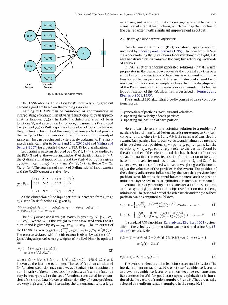
In order to bridge the gap between linearity in the single layerneural network and the highly complex and computationally inten-sive multi-layer neural network, the FLANN architecture with backpropagation learning for classification was proposed (Mishra andDehuri, 2007; Pao, 1989; Pao et al., 1992). FLANN architecture canbe viewed as a non-linear network. In contrast to the linear weight-ing of the input pattern produced by the linear links of the artificialneural network, the functional link acts on an element of a patternor on the entire pattern by generating a set of linearly indepen-dent functions, then evaluating these functions with the pattern asthe argument. Thus class separability is more in the enhanced fea-ture space. A simple FLANN model with a pattern of two features isshown in Fig. 1.

Let us consider a two dimensional input sample x = [x1, x2]T .This sample is mapped to a higher dimensional space by functionalexpansion using trigonometric functions

� = [(x1, sin �x1, sin 2�x1, cos �x1, cos 2�x1),

(x2, sin �x2, sin 2�x2, cos �x2, cos 2�x2)]T .

The weighted sum is defined by

y =∑i,j=1,2

wixj +∑i,j=1,2

wi sin i�xj +∑i,j=1,2

wi cos i�xj. (1)

S. Dehuri et al. / The Journal of Systems a

d

iiftttseD

ttbXa

〈

b

.o

tTya

wkfnmsa

Fig. 1. FLANN for classification.

The FLANN obtains the solution for W iteratively using gradientescent algorithm based on the training samples.

Learning of FLANN may be considered as approximating ornterpolating a continuous multivariate function �(X) by an approx-mating function �w(X). In FLANN architecture, a set of basisunctions �, and a fixed number of weight parameters W are usedo represent �w(X). With a specific choice of set of basis functions �,he problem is then to find the weight parameters W that providehe best possible approximation of � on the set of input–outputamples. This can be achieved by iteratively updating W. The inter-sted reader can refer to Dehuri and Cho (2010a,b) and Mishra andehuri (2007) for a detailed theory of FLANN for classification.

Let k training patterns denoted by 〈 Xi : Yi 〉, 1≤i ≤ k be applied tohe FLANN and let the weight matrix be W. At the ith instant 1≤i ≤ k,he Q-dimensional input pattern and the FLANN output are giveny Xi=〈xi1, xi2, . . ., xiQ〉, 1≤i ≤ k and Yi=[yi], 1≤i ≤ k. Hence X = [X1,2, . . ., Xk]T. The augmented matrix of Q-dimensional input patternnd the FLANN output are given by:

X : Y〉 =

⎛⎜⎝x1,1 x1,2 . x1,Q : y1x2,1 x2,2 . x2,Q : y2. . . . : .xk,1 xk,2 . xk,Q : yk

⎞⎟⎠

As the dimension of the input pattern is increased from Q to Q′

y a set of basis functions , given by

(Xi) = [ 1(xi1), 2(xi1), . . . , 1(xi2), 2(xi2), . . . , 1(xiQ ), 2(xiQ ), . . .= [ 1(xi1), 2(xi2), . . . , Q (xiQ )].

The k × Q dimensional weight matrix is given by W = [W1, W2, . ., Wk]T, where Wi is the weight vector associated with the ithutput and is given by W1 = [wi1, wi2, . . . , wiQ ]. The ith output of

he FLANN is given by yi(t) = ϕ(∑Q ′

j=1 j(xij).wij) = ϕ(Wi . T(Xi)), ∀i.he error associated with the ith output is given by ei(t) = yi(t) −

ˆ i(t). Using adaptive learning, weights of the FLANN can be updateds:

wij(t + 1) = wij(t) + �.�(t),�(t) = ı(t).[ (Xi)],

(2)

here ı(t) = [ı1(t), ı2(t), . . ., ık(t)], ıi(t) = (1 − y2i(t)) · ei(t), � is

nown as the learning parameter. The set of function consideredor function expansion may not always be suitable for mapping the

on-linearity of the complex task. In such cases a few more functionay be incorporated to the set of functions considered for expan-

ion of the input data. However, dimensionality of many problemsre very high and further increasing the dimensionality to a large

nd Software 85 (2012) 1333– 1345 1335

extent may not be an appropriate choice. So, it is advisable to chosea small set of alternative functions, which can map the function tothe desired extent with significant improvement in output.

2.2. Basics of particle swarm algorithms

Particle swarm optimization (PSO) is a nature inspired algorithminvented by Kennedy and Eberhart (1995). Like Leonardo Da Vin-cis work modeling flying machines from watching bird flight, PSOreceived its inspiration from bird flocking, fish schooling, and herdsof animals.

In PSO, a set of randomly generated solutions (initial swarm)propagates in the design space towards the optimal solution overa number of iterations (moves) based on large amount of informa-tion about the design space that is assimilates and shared by allmembers of the swarm. A complete chronicle of the developmentof the PSO algorithm from merely a motion simulator to heuris-tic optimization of the PSO algorithm is described in Kennedy andEberhart (2001, 1995).

The standard PSO algorithm broadly consist of three computa-tional steps:

1. generation of particles’ positions and velocities;2. updating the velocity of each particle;3. updating the position of each particle.

Here, a particle refers to a potential solution to a problem. Aparticle �xk in d-dimensional design space is represented as �xk = 〈 xk1,xk2, xk3,. . ., xkd 〉, where k = 1, 2,. . ., N, N is the number of particles in aswarm. Each particle has its own velocity and maintains a memoryof its previous best position, pk = 〈 pk1, pk2, pk3,. . ., pkd 〉. Let thevelocity �pg = 〈 pg1, pg2, pg3,. . ., pgd 〉 refer to the position found bythe kth member of the neighborhood that has the best performanceso far. The particle changes its position from iteration to iterationbased on the velocity updates. In each iteration �pg and �pk of thecurrent swarm are combined with some weighting coefficients toadjust the velocities of the particles in the swarm. The position ofthe velocity adjustment influenced by the particle’s previous bestposition is considered as the cognition component, and the positioninfluenced by the best in the neighborhood is the social component.

Without loss of generality, let us consider a minimization taskand use symbol f(.) to denote the objective function that is beingminimized. The personal best of the kth particle and the global bestposition can be computed as follows.

�pk(t + 1) ={ �pk(t) if f (�xk(t + 1)) ≥ f (�pk(t))

�xk(t + 1) otherwise, ∀k, k = 1, 2, . . . , N (3)

�pg (t + 1) ={ �pg (t) if ∀k f (�xk(t + 1)) ≥ f (�pg (t))

�xk(t + 1) ifforanyj f (�xj(t + 1)) < f (�pg (t)) , j = 1, 2, . . . , N (4)

In standard PSO algorithm (Kennedy and Eberhart, 1995), at iter-ation t, the velocity and the position can be updated using Eqs. (5)and (6), respectively.

�vk(t + 1) = w ⊗ �vk(t) + �c1 ⊗ �r1(t) ⊗ (�pk(t) − �xk(t)) + �c2 ⊗ �r2(t)

⊗(�pg(t) − �xk(t)) (5)

�xk(t + 1) = �xk(t) + �vk(t + 1) (6)

The symbol ⊗ denotes point by point vector multiplication. Theinertia momentum factor w, (0< w ≤1), self-confidence factor c1

and swarm confidence factor c2 are non-negative real constants.Randomness (useful for good state space exploitation) is intro-duced via the vectors of random numbers �r1 and �r2. They are usuallyselected as a uniform random numbers in the range [0, 1].

1 ems a

rv

cmbstc

|

PtaKoaT

3

spte

3

vbam

�v

x

wraatstapc

sGswt

r

336 S. Dehuri et al. / The Journal of Syst

The original PSO algorithm uses w=1, c1=2, and c2=2. Over yearsesearchers have fined-tuned these parameters and found out aery standard optimized values (Jiang et al., 2007).

These three steps of velocity update, position update, and fitnessomputations are repeated until a desired convergence criterion iset. The stopping criterion is that the maximum change in the

est fitness should be smaller than the specified tolerance for apecified number of iterations, I, as shown in Eq. (7). Alternatively,he algorithm can be terminated when the velocity updates arelose to zero over a number of iterations.

f (�pg(t)) − f (�pg(t − 1))| ≤ ε, t = 2, 3, . . . , I (7)

While empirical evidence has accumulated that the standardSO algorithm works, e.g., it is a useful tool for global optimization,here has thus far been little insight into how it works. In order toddress this, a generalized model has been proposed in Clerc andennedy (2002). Consequently, the convergence and the stabilityf the standard PSO has been proposed by many researches (Berghnd Engelbrecht, 2006; Clerc and Kennedy, 2002; Jiang et al., 2007;relea, 2003).

. ISO-flann for classification

In this section we will discuss the proposed ISO-FLANN for clas-ification. This section is divided into three subsections, namely theroposed improved PSO (IPSO), a general description of its archi-ecture, and a high-level algorithm to measure the computationalfficiency of the proposed architecture.

.1. Improved PSO

The improved PSO algorithm is based on the standard globalersion of the PSO. Like the previous variants of PSO, the draw-acks of PSO with respect to inefficiency in fine tuning solutions,nd a very slow searching around the global optimum inspired ourodifications.The IPSO can be described as follows:

k(t + 1) = ⊗ �vk(t) + �c1 ⊗ �r1(t) ⊗ (�pk(t) − �xk(t))+ �c2 ⊗ �r2(t) ⊗ (�pg(t) − �xk(t)) (8)

�k(t + 1) = �xk(t) + �vk(t + 1) (9)

here is the newly defined adaptive inertia weight. The algo-ithm, by adjusting the parameter , can make reduce graduallys the generation increases. In the searching process of the IPSOlgorithm, the search space will reduce gradually as the genera-ion increases. So the IPSO algorithm is more effective, because theearch space is reduced step by step. The search step length forhe parameter also reduces correspondingly. Similar to geneticlgorithms (GAs) (Goldberg, 1989), after each generation, the bestarticle in the last generation will replaces the worst particle of theurrent generation, thus the better result can be achieved.

In the literature (Eberhart and Shi, 2000; Shi and Eberhart, 1999)everal selection strategies of inertia weight have been given.enerally, in the initial stages of the algorithm, the initial weight hould be reduced rapidly, while around the optimum, the initialeight should be reduced slowly. So in this paper, we adopted

he following procedure:AlgorithmInput: Initial inertia weight = 0; End point of linear section = 1;

Number of generations during which inertial weight iseduced linearly = Gen1;

Maximum generation = Gen2;Reduced ()

nd Software 85 (2012) 1333– 1345

BeginFor i=1:Gen11=0−((1/Gen1)× i);

EndFor i=Gen1+1:Gen21=(0−1)×exp(((Gen1+1)−i)/i);

EndEnd

In particular the value of Gen2 and Gen1 is selected according toempirical knowledge.

Although PSO performs well for global search as it is capableof finding and exploring promising regions in the search space,quickly searching near global optimum is very slow. The self-adaptive evolutionary strategy (ES) is suited for local optimizationdue to its high probability of generating small Gaussian and Cauchyperturbation (Rudolph, 1997; Schwefel, 1981). Thus it is capa-ble of fine-tuning those solutions found by PSO. When the globalbest position of PSO cannot be improved for some successive gen-erations, the self-adaptive ES (Yang and Kao, 2001) is used anenhancement operation of pi and pg . Thus the self adaptive ESfacilitates the convergence of PSO towards global optima. In thisstudy we adapted Schwefel’s (1981) proposal to use self-adaptiveES (i.e., the self adaptive Gaussian and Cauchy mutations) for evolv-ing weight parameters of FLANN.

Self-adaptive Gaussian mutation: Mutation is accomplished byfirst mutating the velocity and then the position of the particle.

vki(t + 1) = vki × exp( ′ × Ngi(0, 1)) + × Nki(0, 1)), (10)

xki(t + 1) = xki(t) + vki(t + 1), (11)

where Ngi(0, 1) is the standard Gaussian density function withrespect to the ith dimension of the global best position of the parti-cle. Similarly Nki(0, 1) is the standard Gaussian density function ofthe ith dimension of the best position found by the particle so far.For this work we follow Bäck and Schwefel (1993) in setting thevalues of = 1/

√2n and = 1/

√2√n, respectively.

Self-adaptive Cauchy mutation: A random variable is said tohave the Cauchy distribution (C(t)), if it has the following densityfunction:

C(t) = t

�(t2 + x2), −∞ < x < +∞. (12)

We will define self adaptive Cauchy mutation as follows:

vki(t + 1) = vki × exp( ′ × Cgi(0, 1)) + × Cki(0, 1)), (13)

xki(t + 1) = xki(t) + vki(t + 1), (14)

where t = 1. In practice, Cauchy mutation is able to make a largerperturbation than Gaussian mutation. This implies that the Cauchymutation has a higher probability of escaping from the local minimathan does Gaussian mutation.

3.2. ISO-FLANN method

ISO-FLANN is a typical three layer feed forward neural networkconsists of an input layer, a hidden layer and an output layer. Theonly difference from FLANN is that, the weight vector is evolved bythe proposed IPSO during the training of the network. Even thoughmany heuristic approaches exist (Goldberg, 1989) for optimizingthe weight vector, we use IPSO because of its characteristics likerapid convergence to global solutions and less number of parame-ters to be optimized. In other words, here we are trying to reducethe local optimal solution of weight vector by IPSO.

The nodes between input and hidden layers are connected with-out weight vector, but the nodes between hidden layer and outputlayer are connected by weights. The signal of the output node isbased on a function of the sum of the inputs to the node.

ems a

tloh

tocpotftr

f

w

b

mfc

s

Taiam

y

f

E

ao

3

naa

Ce

S. Dehuri et al. / The Journal of Syst

In ISO-FLANN architecture, there are d input nodes (i.e., equal tohe number of features of the dataset) and m nodes in the hiddenayer, where m is the number of functionally expanded node andne output neuron in the output layer. The connection betweenidden layer and output layer is assigned with the weight vector.

In this work, we have used the orthonormal trigonometric func-ion for mapping the input feature from one form to another formf higher dimension. However, one can use a function that is verylose to the underlying distribution of the data, but it requires somerior domain knowledge. In this work we are taking five functionsut of which four are trigonometric and one is linear (i.e., keepinghe original form of the feature value). Out of the four trigonometricunctions, two are sine and two are cosine functions. In the case ofrigonometric functions the domain is the given feature values andange lies between [−1,1]. It can be written as

: D → R[−1,1]∪{x}, (15)

here D= {xi1, xi2,. . ., xid}, and d is the number of features.In general let us take f1, f2,. . ., fk as the number of functions to

e used to expand each feature value of the pattern.Therefore, each input pattern can now be expressed as

�xi = {xi1, xi2, . . . , xid} → {{f1(xi1), f2(xi1), . . . , fk(xi1)}, . . . ,{f1(xid), f2(xid), . . . , fk(xid)}, = {{y11, y21, . . . , yk1}, . . . ,{y1d, y2d, . . . , ykd}}.

The weight vector between hidden layer and output layer isultiplied with the resultant sets of non-linear outputs and are

ed to the output neuron as an input. Hence the weighted sum isomputed as follows:

=m∑j=1

yij · wj, i = 1, 2, . . . , Nand m be the total number

of expanded features. (16)

The network has the ability to learn through training by IPSO.he training requires a set of training data, i.e., a series of inputnd associated output vectors. During the training, the networks repeatedly presented with the training data and the weightsdjusted by IPSO from time to time till the desired input–outputapping occurs.The estimated output is then computed by the following metric:

ˆ i(t) = f (si), i = 1, 2, . . . , N.

The error ei(t) = yi(t)−yi(t), i = 1, 2,. . ., N is the error obtainedrom the ith pattern of the training set.

Therefore the error criterion function can be written as,

(t) =N∑i=1

ei(t), (17)

nd our objective is to minimize this function with an optimal setf weights.

.3. ISO-FLANN high-level algorithm

ISO-FLANN, a member of the family of higher order neuraletworks, is a computational model capable of learning throughdjustment of internal weight parameters according to a training

lgorithm in response to some training examples.

There are many literatures exist (Carvalho and Ludermir, 2007;hang et al., 2007; Da and Xiurun, 2005; Wu et al., 2006; John Pault al., 2006) on PSO-based neural network training, but to the best

nd Software 85 (2012) 1333– 1345 1337

of our knowledge IPSO-based FLANN training and its application toclassification problem is the first effort in this direction.

In ISO-FLANN the weights between hidden and output layer isadaptively evolved by IPSO algorithm, starting from the parents’weights instead of randomly initialized weights, so this can prefer-ably solve the problem of noisy fitness evaluation that can misleadthe evolution.

The dataset is divided into two mutually exclusive sets: a train-ing set and a test set (more details in Section 4). The training setis used to evolve the optimal model with optimal sets of weightsusing IPSO, and the fitness evaluation is based on the error crite-rion function E, which is already described in Section 3.2. In orderto embed IPSO for weight evolution one could keep the follow-ing points in mind: the particle representation, and the objectivefunction to measure the effectiveness of the particle.

3.3.1. Representation of a particleFor the evolutionary process, the length of each and every par-

ticle is m and it is fixed (i.e., the number of connection betweenexpanded features of the hidden layer and the output neuron of theoutput layer), but one can go for variable length particle also. Thevariable length particle representation is highly useful for simulta-neous evolution of architectures and weights. In this work our focusis on fixed length particle, the variable length particle is beyond thescope of our study. A particle can be represented as a vector of mweights, i.e., 〈 w1, w2, w3,. . ., wm 〉.

In ISO-FLANN the weight values lie between [−1, 1]. Hence thevelocity of the particle also lies between [−1, 1]. In case of extremevalues like wi = 0, one can believe that the connection between theexpanded features and output node corresponding to wi is not aninformative one and is virtually deleted from the network.

3.3.2. Objective functionDuring evolution each particle measures its effectiveness by the

error criterion function, using Eq. (17) mentioned in Section 3.2.The major steps of EFLANN can be described as follows:

1. DIVISION OF DATASETDivide the dataset into two parts: training and testing.

2. MAPPING OF INPUT PATTERNSMap each pattern from lower dimension to higher dimension,i.e., expand each feature value according to predefined set offunctions.

3. RANDOM INITIALIZATIONInitialize each particle randomly with small values from thedomain [−1, 1].

4. WHILE(Termination Criterion Not Met)FOR entire swarm

FOR each particle in the swarmFOR each sample of training sample

Calculate the weighted sum and feed as an input tothe node of the output layer.Calculate the error and accumulate it.

ENDFitness of the particle is equal to the accumulated error.If fitness value is better than the best fitness value inhistory, set current value as the new personal best,

ENDChoose the particle with best fitness value of all the par-ticles as the global best.

FOR each particle

Call Reduced () and calculate particle velocity accord-ing to Eq. (8).Update Particle position according to Eq. (9).

END

1 ems a

5

abtcoa

4

ceuwdl

paom

dsapc

4

s

t(ceaiaa

odpi2aa

oIaid

338 S. Dehuri et al. / The Journal of Syst

ENDMUTATIONApply Cauchy and Gaussian mutation if the position of theglobal best solution is not improved for a successive numberof pre-specified generations alternatively by using Eqs. (11)and (14).

. WHILE END

This algorithm does not optimizing the weight vector only butlso implicitly optimizing the required number of connectionsetween hidden layer and output layer. Hence we can say this is aype of architecture optimization. However, in this work we are notonsidering this issue. Hence, instead of a multi-objective functionptimization we are only optimizing the uni-objective, i.e., knowns classification accuracy.

. Experimental details

Even though the proposed algorithm is primarily intended forlassification of datasets with large number of records and a mod-rate number of features (primarily for data mining), it can also besed very well on more conventional datasets. To exhibit this facte evaluated our algorithm using a set of fifteen public domainatasets from the University of California at Irvine (UCI) machine

earning repository (Blake and Merz, 2012).We have compared the results of ISO-FLANN with other com-

eting classification methods such as multi-layer perception (MLP)nd the FLANN with gradient descent (and with the same setf orthonormal basis functions like ISO-FLANN), support vectorachine (SVM) with radial basis kernel and FSN.This section is divided into three subsections. Section 4.1

iscusses the nature and characteristics of the datasets being clas-ified. The environment, parameter setting of the proposed methodlong with the methods considered for comparative study and theerformance of the model is demonstrated in Section 4.2 with a dis-ussion. Finally a comparative performance is given in Section 4.3.

.1. Description of the datasets

Let us briefly discuss the datasets, chosen for our experimentaletup.

IRIS Datasets: This is the most popular and simple classifica-ion dataset based on multivariate characteristics of a plant specieslength and thickness of petal and sepal) divided into three distinctlasses(Iris Setosa, Iris Versicolor, and Iris Virginica) of 50 instancesach. One class is linearly separable from the other two; the latterre not linearly separable from each other. In a nutshell, it has 150nstances and 5 attributes. Out of Five attributes, Four attributesre predicting attributes and one is goal attribute. All the predictingttributes are real values.

WINE Dataset: This dataset is resulted from a chemical analysisf wines grown in the same region in Italy but derived from threeifferent cultivars. In classification context, this is a well-posedroblem with well-behaved class structures. The total number of

nstances is 178 and it is distributed as 59 for class 1, 71 for class and 48 for class 3. The number of attributes is 14 including classttribute and all 13 are continuous in nature. There are no missingttribute values in this dataset.

PIMA Indians Diabetes Data base: This database is a collectionf all female patients of at least 21 years of PIMA Indian heritage.

t contains 768 instances, 2 classes of positive and negative and 9ttributes including the class attribute. The attribute contains eithernteger or real values. There are no missing attribute values in theataset.

nd Software 85 (2012) 1333– 1345

BUPA Liver Disorders: This Dataset related to the diagnosis of liverdisorders and created by BUPA Medical Research, Ltd. It consists of345 records, 7 attributes including the class attributes. The classattribute is repeated with only two class values for entire database.The first 5 attributes are all blood tests, which are thought to besensitive to liver disorders that might arise from excessive alcoholconsumption. Each record corresponds to a single male individual.

Clevend Heart disease: This dataset is related to diagnoses ofpeople with heart problems. It consists of 304 data instances, 5attributes including the class and 2 classes.

Wisconsin Diagnostic Breast Cancer (WBC (D)): This dataset isrelated to diagnosis of people with breast cancer. Features of thedataset are computed from a digitized image of a fine needle aspi-rate (FNA) of a breast mass. They describe characteristics of thecell nuclei present in the image. The dataset has 569 instances, 32attributes and 2 classes namely, benign and malignant.

Wisconsin prognostic Breast Cancer (WBC (D)): This dataset isrelated to diagnosis of people with breast cancer. Each record rep-resents follow-up data for one breast cancer case. The dataset has198 instances, 30 attributes and 2 classes namely, recurrent andnon-recurrent. Out of the 198 instances 4 instances have missingvalues.

Page Block: This dataset is used for classifying all the blocks of thepage layout of a document that has been detected by a segmenta-tion process. This is an essential step in document analysis in orderto separate text from graphic areas. Indeed, the five classes are:text (1), horizontal line (2), picture (3), vertical line (4) and graphic(5). The dataset consist of 5473 instances and 10 attributes. Theattributes are combination of integer and float values. The datasethave no missing values.

Thyroid: This dataset is used to predict whether a patient’s thy-roid to the class euthyroidism (normal), hypothyroidism (Hypo) orhyperthyroidism (hyper). The diagnosis (the class label) was basedon a complete medical record, including anamnesis, scan etc. Thedataset had 215 instances with no missing values and 5 attributes.All the attributes are of continuous nature.

Metabolic Syndrome: The metabolic syndrome dataset (Parkand Cho, 2006) is obtained from Yonchon County of Korea. Themetabolic syndrome is a collection of metabolic disorder whichincludes hypertension, dyslipidemia, elevated blood glucose andobesity. The dataset have 1135 samples with 2 class labels. Thedataset has 18 attributes and the class attribute determine theabsence or presence of the disease. The attributes of the datasethave a combination of categorical and continuous values. Thedataset doesn’t have any missing values. 11 important attributewhich are necessary for the prediction.

Dermatology: This dataset is obtained from the diagnosis of thepatients of erythemato-squamous diseases. The diseases in thisgroup are psoriasis, seboreic dermatitis, lichen planus, pityriasisrosea, cronic dermatitis, and pityriasis rubra pilaris. This datasetis obtained by evaluating clinically with 12 features. Afterwards,skin samples were taken for the evaluation of 22 histopathologicalfeatures.

Hepatitis: This dataset is used for classification of hepatitispatients into two classes labeled as ‘Die’ and ‘Live’ based onthe pathological analysis. The dataset has 20 attributes and 157instances.

Parkinson: This dataset is composed of a range of biomedicalvoice measurements from 31 people, 23 with Parkinson’s disease(PD). Each column in the table is a particular voice measure, andeach row corresponds one of 195 voice recording from differentindividuals. The main aim of the data is to discriminate healthy

people from those with PD, according to “status” column which isset to 0 for healthy and 1 for PD.

Vertebral column: This dataset is obtained from Group of AppliedResearch in Orthopaedics (GARO), Lyon, France. This dataset is

S. Dehuri et al. / The Journal of Systems and Software 85 (2012) 1333– 1345 1339

Table 1Summarized view of characteristics of the dataset.

Dataset Number ofpatterns

Number offeatures

Number ofclasses

Number ofpatterns inclass 1

Number ofpatterns inclass 2

Number ofpatterns inclass 3

Number ofpatterns inclass 4

Number ofpatterns inclass 5

Numberpatterns inclass 6

Page Block 5473 10 5 4913 329 28 88 115IRIS 150 5 3 50 50 50WINE 178 14 3 71 59 48Thyroid 215 5 3 150 35 30PIMA 768 9 2 500 268BUPA 345 7 2 145 200Clevend Heart 304 6 2 45 259WBC (D) 569 30 2 357 212WBC (P) 194 32 2 148 46Metabolic Syndrome 1135 18 2 612 523Dermatology 366 33 6 112 61 72 49 52 20Hepatitis 155 19 2 32 123

ult

ot“tc

dtrni

4

4

pp2mr

aotfs9

4

fua

sdpfio

sa

value is decreased accordingly. In this work we stop a run eitherthe points in P are identical to an accuracy of three decimal places,i.e., |fmin − fopt| ≤ ε = 10−3, or the maximum number of generationsGen2 = 3000.

Table 2Parameters used in proposed algorithm.

Symbol Name and purpose of the parameter

N Size of the swarm (P) Inertia weight0 Inertial value of inertia weight Inertia weight value of the end point of linear section

Parkinson 196 23 2 48

Ionosphere 351 34 2 225

Vertebral column 310 6 2 100

sed for classification task. It classifies patients into two categoriesabeled as ‘normal’ and ‘abnormal’ based on the analysis report ofheir vertebral column.

Ionosphere: This radar dataset is used for classifying the presencef electrons structure in the ionosphere. “Good” radar returns arehose showing evidence of some type of structure in the ionosphere.Bad” returns are those that do not; their signals pass throughhe ionosphere. The dataset consist of 34 of attributes which areontinuous in nature.

Table 1 presents a summary of the main characteristics of theatabases that have been used in this study. The first column of thisable gives the name of the database, while other columns indicate,espectively, the number of instances, the number of attributes,umber of classes, number of patterns in class 1, number of patterns

n class 2 and number of patterns in class 3.

.2. Environments, parameters and classification performance

.2.1. EnvironmentsThe proposed method was implemented on a personal com-

uter with an Intel Pentium IV, 2.40 GHz CPU, 1.00 GB RAM (therimary method), the Microsoft Windows XP Professional version002 operating system with Matlab 7.0.1 development environ-ent. For evaluating all these algorithms, the following protocols

elated to dataset division were set.The datasets are divided into 10 folds, and out of this 9-folds

re used for training and 1 fold is used for testing the performancef the classifiers. However, 9-fold cross validation is carried out inhe case of HEART disease database obtained from STATLOG projector comparing the cost estimation result of ISO-FLANN with othertate-of-the-art algorithms presented in King et al. (1995) where-fold cross validation was reported.

.2.2. ParametersThe quality of each particle is measured by the error criterion

unction E. It is also very important for the user to set a priori the val-es of the parameters of the proposed algorithm. These parametersre presented in Table 2.

In the literature different values of N have been used for swarmize. In this work we set N = 10×d to avoid under-fit and over-fituring the training of the algorithm. The larger is the number ofarticles, more is the computation time. Length of the particle isxed to m, where m depends on the functionally expanded features

f the hidden layer.

Although the parameters are quite restricted and there are nouch standard rule to assign systematic parameter values to c1, c2nd but in this experimental study the value of is restricted

148126210

within the interval [1.8, 0.2]. The values of c1 and c2 are chosenas 2.8 × and 1.3 ×, respectively. These set of parameters areassigned after an extensive set of trial and error process.

The initial position and the velocity range of the particles in IPSOlies in the interval [−1, +1] and if the global best position pg is notimproved for successive generations (100) we run the self adap-tive Gaussian and Cauchy mutation alternatively to escape fromthe false global solution (i.e., the equivalent of a local optimum inglobal optimization).

The next important question in the proposed IPSO is when tostop a run. Many researchers have used either the maximum num-ber of generations (Gen2) or maximum number of function calls asstopping conditions in their experimental study (Blake and Merz,2012). Liu et al. (2005) used |fmin − fopt| ≤ ε, where fmin is the bestsolution found so far. The stopping condition |fmin − fopt| ≤ ε onlyapplies if the optimal value of the problem under consideration isknown. However, in many practical applications, the optimal valueis not known. On other hand, the maximum number of iterations(orfunction calls) cannot be judged for an arbitrary decision boundaryof a classification problem. This may lead to unnecessary functioncalls when the minimum is reached long before the maximum num-ber of iterations (or function calls)—thus increasing computationalcosts. In this paper we use a combined approach as follows:

In each iteration we check the condition |fmin − fopt| ≤ ε, wherefw=f(pi) is the functional value of current worst personal best pi inP and fb=f(pg) is the functional value of the current global best pg

in P (since each particle in P is always updated with an improve-ment at each iteration, the set P will gradually contract) and Gen1and Gen2. If this condition is reached earlier than Gen2, then stop.Otherwise continue till the value of Gen2 is reached. However, theGaussian and Cauchy mutation is applied as usual and the inertia

1

Gen1 Generations that reduces linearly (i.e., Gen1 = Gen2 × 40%)Gen2 Maximum generation of the algorithmc1 Cognitive parameterc2 Social parameter

1340 S. Dehuri et al. / The Journal of Systems and Software 85 (2012) 1333– 1345

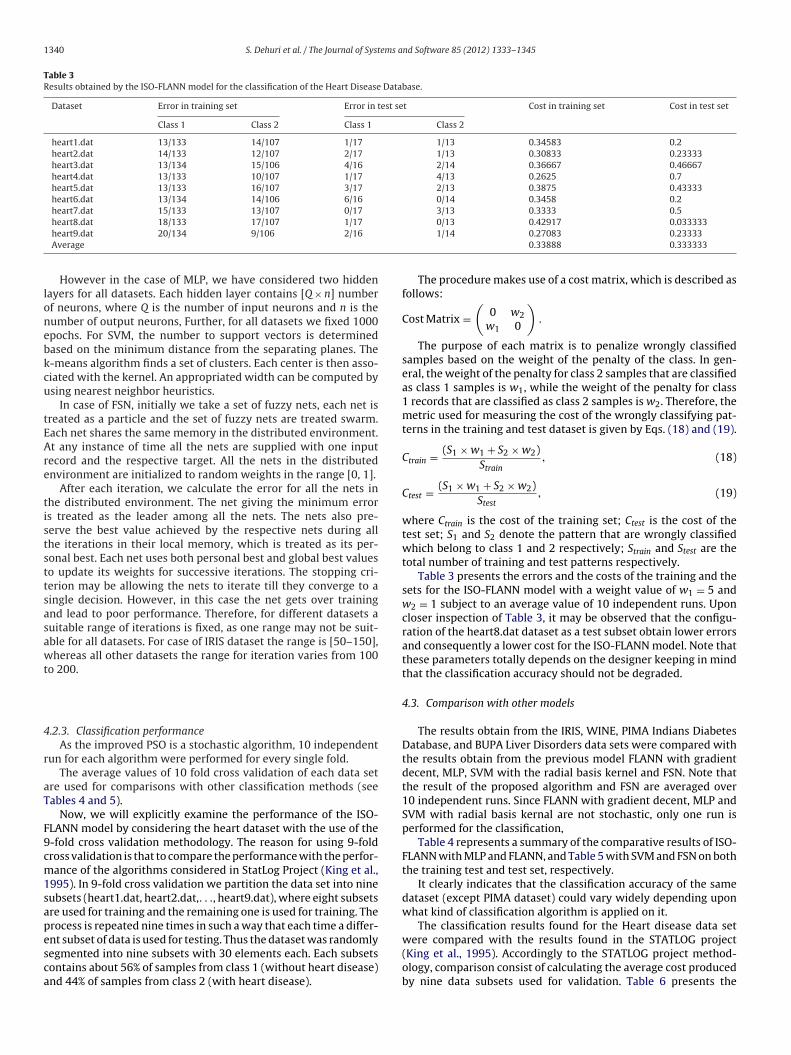
Table 3Results obtained by the ISO-FLANN model for the classification of the Heart Disease Database.

Dataset Error in training set Error in test set Cost in training set Cost in test set

Class 1 Class 2 Class 1 Class 2

heart1.dat 13/133 14/107 1/17 1/13 0.34583 0.2heart2.dat 14/133 12/107 2/17 1/13 0.30833 0.23333heart3.dat 13/134 15/106 4/16 2/14 0.36667 0.46667heart4.dat 13/133 10/107 1/17 4/13 0.2625 0.7heart5.dat 13/133 16/107 3/17 2/13 0.3875 0.43333heart6.dat 13/134 14/106 6/16 0/14 0.3458 0.2heart7.dat 15/133 13/107 0/17 3/13 0.3333 0.5

lonebkcu

tEAre

tiststtsasawt

4

r

aT

F9cm1sapesca

heart8.dat 18/133 17/107 1/17

heart9.dat 20/134 9/106 2/16

Average

However in the case of MLP, we have considered two hiddenayers for all datasets. Each hidden layer contains [Q × n] numberf neurons, where Q is the number of input neurons and n is theumber of output neurons, Further, for all datasets we fixed 1000pochs. For SVM, the number to support vectors is determinedased on the minimum distance from the separating planes. The-means algorithm finds a set of clusters. Each center is then asso-iated with the kernel. An appropriated width can be computed bysing nearest neighbor heuristics.

In case of FSN, initially we take a set of fuzzy nets, each net isreated as a particle and the set of fuzzy nets are treated swarm.ach net shares the same memory in the distributed environment.t any instance of time all the nets are supplied with one inputecord and the respective target. All the nets in the distributednvironment are initialized to random weights in the range [0, 1].

After each iteration, we calculate the error for all the nets inhe distributed environment. The net giving the minimum errors treated as the leader among all the nets. The nets also pre-erve the best value achieved by the respective nets during allhe iterations in their local memory, which is treated as its per-onal best. Each net uses both personal best and global best valueso update its weights for successive iterations. The stopping cri-erion may be allowing the nets to iterate till they converge to aingle decision. However, in this case the net gets over trainingnd lead to poor performance. Therefore, for different datasets auitable range of iterations is fixed, as one range may not be suit-ble for all datasets. For case of IRIS dataset the range is [50–150],hereas all other datasets the range for iteration varies from 100

o 200.

.2.3. Classification performanceAs the improved PSO is a stochastic algorithm, 10 independent

un for each algorithm were performed for every single fold.The average values of 10 fold cross validation of each data set

re used for comparisons with other classification methods (seeables 4 and 5).

Now, we will explicitly examine the performance of the ISO-LANN model by considering the heart dataset with the use of the-fold cross validation methodology. The reason for using 9-foldross validation is that to compare the performance with the perfor-ance of the algorithms considered in StatLog Project (King et al.,

995). In 9-fold cross validation we partition the data set into nineubsets (heart1.dat, heart2.dat,. . ., heart9.dat), where eight subsetsre used for training and the remaining one is used for training. Therocess is repeated nine times in such a way that each time a differ-

nt subset of data is used for testing. Thus the dataset was randomlyegmented into nine subsets with 30 elements each. Each subsetsontains about 56% of samples from class 1 (without heart disease)nd 44% of samples from class 2 (with heart disease).

0/13 0.42917 0.0333331/14 0.27083 0.23333

0.33888 0.333333

The procedure makes use of a cost matrix, which is described asfollows:

Cost Matrix =(

0 w2w1 0

).

The purpose of each matrix is to penalize wrongly classifiedsamples based on the weight of the penalty of the class. In gen-eral, the weight of the penalty for class 2 samples that are classifiedas class 1 samples is w1, while the weight of the penalty for class1 records that are classified as class 2 samples is w2. Therefore, themetric used for measuring the cost of the wrongly classifying pat-terns in the training and test dataset is given by Eqs. (18) and (19).

Ctrain = (S1 × w1 + S2 × w2)Strain

, (18)

Ctest = (S1 × w1 + S2 × w2)Stest

, (19)

where Ctrain is the cost of the training set; Ctest is the cost of thetest set; S1 and S2 denote the pattern that are wrongly classifiedwhich belong to class 1 and 2 respectively; Strain and Stest are thetotal number of training and test patterns respectively.

Table 3 presents the errors and the costs of the training and thesets for the ISO-FLANN model with a weight value of w1 = 5 andw2 = 1 subject to an average value of 10 independent runs. Uponcloser inspection of Table 3, it may be observed that the configu-ration of the heart8.dat dataset as a test subset obtain lower errorsand consequently a lower cost for the ISO-FLANN model. Note thatthese parameters totally depends on the designer keeping in mindthat the classification accuracy should not be degraded.

4.3. Comparison with other models

The results obtain from the IRIS, WINE, PIMA Indians DiabetesDatabase, and BUPA Liver Disorders data sets were compared withthe results obtain from the previous model FLANN with gradientdecent, MLP, SVM with the radial basis kernel and FSN. Note thatthe result of the proposed algorithm and FSN are averaged over10 independent runs. Since FLANN with gradient decent, MLP andSVM with radial basis kernal are not stochastic, only one run isperformed for the classification,

Table 4 represents a summary of the comparative results of ISO-FLANN with MLP and FLANN, and Table 5 with SVM and FSN on boththe training test and test set, respectively.

It clearly indicates that the classification accuracy of the samedataset (except PIMA dataset) could vary widely depending uponwhat kind of classification algorithm is applied on it.

The classification results found for the Heart disease data set

were compared with the results found in the STATLOG project(King et al., 1995). Accordingly to the STATLOG project method-ology, comparison consist of calculating the average cost producedby nine data subsets used for validation. Table 6 presents the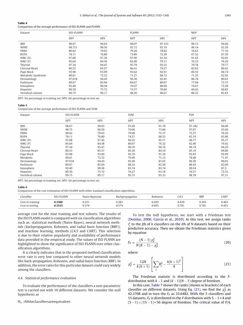

S. Dehuri et al. / The Journal of Systems and Software 85 (2012) 1333– 1345 1341

Table 4Comparison of the average performance of ISO-FLANN and FLANN.

Dataset ISO-FLANN FLANN MLP

HPT HPS HPT HPS HPT HPS

IRIS 98.67 99.03 98.07 97.333 98.15 94.00WINE 98.751 96.56 92.72 92.19 96.14 92.29PIMA 80.62 79.63 79.20 78.82 76.61 77.19BUPA 78.11 76.80 73.80 72.29 67.52 67.39WBC (D) 97.68 97.36 97.96 91.54 91.62 92.65WBC (P) 85.64 84.36 82.06 79.11 76.32 76.29Thyroid 97.34 94.47 95.78 93.25 79.78 79.77Clevend Heart 86.53 85.57 86.41 79.27 82.63 80.42Page block 93.98 93.09 93.62 92.91 86.55 84.74Metabolic Syndrome 80.61 72.32 71.27 68.72 71.35 62.92Dermatology 97.018 94.43 96.36 92.45 86.78 80.63Parkinson 89.67 85.94 84.67 80.97 77.04 73.75Ionosphere 92.40 90.38 79.67 80.94 74.61 73.28Hepatitis 80.39 75.72 73.57 70.60 60.42 60.83Vertebral column 99.75 99.17 98.26 96.67 88.32 85.83

HPT: hit percentage in training set, HPS: hit percentage in test set.

Table 5Comparison of the average performance of ISO-FLANN and SVM.

Dataset ISO-FLANN SVM FSN

HPT HPS HPT HPS HPT HPS

IRIS 98.67 99.03 91.69 91.70 97.182 96.00WINE 98.75 96.56 79.06 73.66 97.87 93.69PIMA 80.62 79.63 79.68 75.37 75.27 76.39BUPA 78.11 76.80 74.57 68.53 65.19 65.00WBC (D) 97.68 97.36 96.55 95.71 96.77 95.27WBC (P) 85.64 84.38 80.07 76.32 82.46 79.42Thyroid 97.34 95.47 90.70 90.76 96.74 94.39Clevend Heart 86.53 85.57 85.20 84.19 85.19 84.86Page block 93.98 93.09 92.70 91.39 92.83 92.09Metabolic 80.61 72.32 79.49 71.12 78.48 71.47Dermatology 97.018 94.43 95.49 87.65 96.28 90.65Parkinson 89.67 85.94 88.32 82.50 88.43 83.69Ionosphere 92.40 90.38 83.74 83.74 90.54 87.5Hepatitis 80.39 75.72 76.27 63.18 76.57 72.52Vertebral column 99.75 99.17 95.75 93.33 98.78 97.31

HPT: hit percentage in training set, HPS: hit percentage in test set.

Table 6Comparison of the cost estimation of ISO-FLANN with other standard classification algorithms.

propa

1

4

atsoaidhs

elaa

4

th

H

Classifier ISO-FLANN Naive Bayesian Back

Cost in training 0.3388 0.351 0.38Cost in testing 0.3333 0.374 0.57

verage cost for the nine training and test subsets. The results ofhe ISO FLANN model is compared with six classification algorithmsuch as: statistical methods (Naive Bayes), neural network meth-ds (backpropagation, Kohonen, and radial basis function (RBF)),nd machine learning, methods (C4.5 and CART). This selections due to their relative popularity and availability of performanceata provided in the empirical study. The values of ISO FLANN areighlighted to show the significance of ISO-FLANN over other clas-ification algorithms.

It is clearly indicates that in the proposed method classificationrror rate is very low compared to other neural network modelsike back-propagation, Kohonen, and radial basis function (RBF). Inddition, the error rates for this particular dataset could vary widelymong the classifiers.

.4. Statistical performance evaluation

To evaluate the performance of the classifiers a non-parametric

est is carried out with 10 different datasets. We consider the nullypothesis as

o :Alltheclassifiersareequivalent.

gation Kohonen C4.5 RBF CART

0.429 0.439 0.303 0.4630.693 0.781 0.781 0.452

To test the null hypothesis, we start with a Friedman test(Demsar, 2006; García et al., 2010). In this test, we assign ranksrji

to the jth of k classifiers on the ith of N datasets based on theirpredictive accuracy. Then we obtain the Friedman statistics givenby equation

FF = (N − 1)�2F

N (K − 1) − �2F

(20)

where

�2F = 12N

k (k + 1)

⎡⎣∑

j

R2j − k(k + 1)2

4

⎤⎦ (21)

The Friedman statistic is distributed according to the F-distribution with k − 1 and (k − 1)(N − 1) degree of freedom.

In this case, Table 7 shows the ranks (shown in brackets) of each

classifier on different datasets. Using Eq. (21), we find the �2

F as42.3708 and in turn the FF as 33.6482. With the 5 classifiers and15 datasets, FF is distributed to the F distribution with 5 − 1 = 4 and(5 − 1) × (15 − 1) = 56 degree of freedom. The critical value of F(4,

1342 S. Dehuri et al. / The Journal of Systems and Software 85 (2012) 1333– 1345

Table 7Ranks of each classifiers on different dataset based on the average hits percentage on test set.

Dataset ISO-FLANN FLANN FSN MLP SVM

IRIS 99.03 (1) 97.33 (2) 96.00 (3) 94.00 (4) 91.70 (5)WINE 96.56 (1) 92.19(4) 93.69 (2) 92.29 (3) 73.66 (5)PIMA 79.63 (1) 78.82 (2) 75.37 (5) 77.19 (3) 76.39 (4)BUPA 76.80 (1) 72.29 (2) 68.53 (3) 67.39 (4) 65.00 (5)WBC (D) 97.36 (1) 91.54 (5) 95.26 (3) 92.65 (4) 95.71 (2)WBC (P) 84.38 (1) 79.11 (3) 79.421 (2) 76.29 (5) 76.32 (4)Page block 93.09(1) 92.91 (2) 92.09 (3) 84.74 (5) 91.39 (4)Thyroid 95.47 (1) 93.25 (3) 94.39 (2) 79.77 (5) 90.76 (4)Clevend heart 85.57 (1) 79.27 (5) 84.86 (2) 80.42 (4) 84.19 (3)Metabolic syndrome 72.32 (1) 68.72 (4) 71.47 (2) 62.92 (5) 71.12 (3)Dermatology 94.28 (1) 92.45 (2) 90.65 (3) 80.63 (5) 87.65 (4)Hepatitis 75.72 (1) 70.60 (3) 72.52 (2) 60.83 (5) 63.18 (4)Parkinson 85.94 (1) 80.97 (4) 83.69 (2) 73.75 (5) 82.50 (3)

5T

hepc

z

w

S

tp

H

Wfppwih

4

aafiuwsmFatvata

o[

ISO-FLANN

The proposed structure with functional expansion usingtrigonometric functions has the following advantages:

Ionosphere 90.38(1) 80.94(4)

Vertebral Column 99.17 (1) 96.67 (3)

Average 1 3.2

6) for = 0.01 as 3.674 which is less than the obtain FF statistic.hus, we can reject the null hypothesis Ho.

As the null hypothesis is rejected, we proceed with the postoc test. We perform the Holm procedure (Demsar, 2006; Garcíat al., 2010; Luengo et al., 2009) to evaluate performance of pro-osed model with other classifier. For carrying this test, we need toompute the z value using Eq. (22)

= Ri − RjSE

(22)

here

E =√k(k + 1)

6N(23)

This z value is used for calculating the probability p from theable of normal distribution, which then compared with an appro-riate ˛. For this test, we consider the null hypothesis as

o :The pair of classifiers compared are equivalent.

e order the p values in increasing order of significance and thenor Holm test, we compare the pi value with ˛/(k − i). The value ofi is less than the ˛/(k − i), thus, we reject the null hypothesis androceed for comparison with other classifiers. The result of this testith ISO-FLANN and other classifiers is shown in Table 8. From this,

t is clear that all the null-hypothesis are rejected. Thus ISO-FLANNas significantly better performance than all other classifiers.

.5. Effect of parameters on classification accuracy

The parameters used in ISO-FLANN effects the classificationccuracy of different datasets. So, a fine tuning of the parametersre important for attaining the optimal classification accuracy. Therst parameter considered is the inertia weight which is adjustedsing Reduced method. In the Reduced method, the initial inertiaeight reduces rapidly for Gen1 and then inertia weight is reduces

lowly for Gen2. The Gen1 is equal to xofGen2 where the x is deter-ined empirically. Fig. 2 shows the effect of change in the x values.

rom the figure, it can be seen that on increasing the x, the trainingccuracy of clevend heart and metabolic dataset increases. But theesting accuracy increases for [0.4-0.5], but further increasing thealue of x, i.e., if the inertia weight is reduced rapidly, the testingccuracy decreases. Almost for all the ten dataset, we have seenhat if Gen1 = [0.4 − 0.5] × Gen2, then maximum accuracy can be

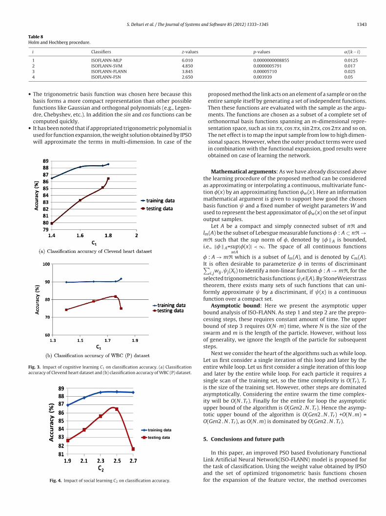
chieved.

We have seen similar effect of the cognitive learning factor (C1)n classification accuracy. If the C1 is considered in the range of1.7–1.8], then a maximum classification accuracy can be achieved.

87.5 (2) 63.28 (5) 83.74 (3)97.31 (2) 85.83 (5) 93.33 (4)

2.53 4.47 3.8

Fig. 3 shows the impact of C1 on classification accuracy. Here thetraining accuracy increases linearly for both the clevend heart andWisconsin prognostic breast cancer dataset, however, the samecannot be seen in testing accuracy of the Wisconsin prognosticbreast cancer dataset. So, we need to fine tune the C1 parametercarefully.

The impact of Social learning factorC2 is same for almost alldataset. The classification accuracy increases till C2 = 2.5, but on fur-ther increasing it the accuracy decreases. The same effect is seen inall the dataset. The representative sample of the effect is shown inFig. 4.

4.6. Justification of trigonometric basis and asymptotic bound of

Fig. 2. Impact of percentage change in Gen1 on classification accuracy. (a) Classifi-cation accuracy of Clevend heart dataset and (b) classification accuracy of MetabolicSyndrome dataset.

S. Dehuri et al. / The Journal of Systems and Software 85 (2012) 1333– 1345 1343

Table 8Holm and Hochberg procedure.

i Classifiers z-values p-values ˛/(k − i)

1 ISOFLANN-MLP 6.010 0.0000000008855 0.0125

•

•

Fa

2 ISOFLANN-SVM 4.8503 ISOFLANN-FLANN 3.8454 ISOFLANN-FSN 2.650

The trigonometric basis function was chosen here because thisbasis forms a more compact representation than other possiblefunctions like Gaussian and orthogonal polynomials (e.g., Legen-dre, Chebyshev, etc.). In addition the sin and cos functions can becomputed quickly.

It has been noted that if appropriated trigonometric polynomial isused for function expansion, the weight solution obtained by IPSOwill approximate the terms in multi-dimension. In case of the

ig. 3. Impact of cognitive learning C1 on classification accuracy. (a) Classificationccuracy of Clevend heart dataset and (b) classification accuracy of WBC (P) dataset.

Fig. 4. Impact of social learning C2 on classification accuracy.

0.0000005791 0.0170.00005710 0.0250.003939 0.05

proposed method the link acts on an element of a sample or on theentire sample itself by generating a set of independent functions.Then these functions are evaluated with the sample as the argu-ments. The functions are chosen as a subset of a complete set oforthonormal basis functions spanning an m-dimensional repre-sentation space, such as sin �x, cos �x, sin 2�x, cos 2�x and so on.The net effect is to map the input sample from low to high dimen-sional spaces. However, when the outer product terms were usedin combination with the functional expansion, good results wereobtained on case of learning the network.

Mathematical arguments: As we have already discussed abovethe learning procedure of the proposed method can be consideredas approximating or interpolating a continuous, multivariate func-tion �(x) by an approximating function �w(x). Here an informationmathematical argument is given to support how good the chosenbasis function and a fixed number of weight parameters W andused to represent the best approximator of �w(x) on the set of inputoutput samples.

Let A be a compact and simply connected subset of nR andlm(A) be the subset of Lebesgue measurable functions � : A ⊂ nR →mR such that the sup norm of �, denoted by ‖� ‖ A is bounded,i.e., ‖� ‖ A=sup

x�A|�(x)| ≺ ∞. The space of all continuous functions

� : A → mR which is a subset of lm(A), and is denoted by Cm(A).It is often desirable to parameterize � in terms of discriminant∑

i,jwij. j(Xi) to identify a non-linear function � : A → mR, for theselected trigonometric basis functions i�l(A). By StoneWeierstrasstheorem, there exists many sets of such functions that can uni-formly approximate by a discriminant, if (x) is a continuousfunction over a compact set.

Asymptotic bound: Here we present the asymptotic upperbound analysis of ISO-FLANN. As step 1 and step 2 are the prepro-cessing steps, these requires constant amount of time. The upperbound of step 3 requires O(N · m) time, where N is the size of theswarm and m is the length of the particle. However, without lossof generality, we ignore the length of the particle for subsequentsteps.

Next we consider the heart of the algorithms such as while loop.Let us first consider a single iteration of this loop and later by theentire while loop. Let us first consider a single iteration of this loopand later by the entire while loop. For each particle it requires asingle scan of the training set, so the time complexity is O(Tr), Tr

is the size of the training set. However, other steps are dominatedasymptotically. Considering the entire swarm the time complex-ity will be O(N . Tr). Finally for the entire for loop the asymptoticupper bound of the algorithm is O(Gen2 . N . Tr). Hence the asymp-totic upper bound of the algorithm is O(Gen2 . N . Tr) +O(N . m) =O(Gen2 . N . Tr), as O(N . m) is dominated by O(Gen2 . N . Tr).

5. Conclusions and future path

In this paper, an improved PSO based Evolutionary Functional

Link Artificial Neural Network(ISO-FLANN) model is proposed forthe task of classification. Using the weight value obtained by IPSOand the set of optimized trigonometric basis functions chosenfor the expansion of the feature vector, the method overcomes

1 ems a

tasdtErFlgt

apcgm

R

B

B

B

C

C

C

D

D

D

D

D

D

E

G

G

G

G

H

H

344 S. Dehuri et al. / The Journal of Syst

he non-linearity of the classification problem. Further the self-daptivity Gaussian and Cauchy mutation can further fine-tune theolutions found by the proposed algorithm. Experimental studyemonstrated that the performance of ISO-FLANN for classifica-ion task is promising. In most cases, the result obtained with theFLSNN model proved to be as good as or better than the bestesults found by the MLP, SVM, FLANN with gradient decent andSN. The architectural complexity of the ISO-FLANN model is quiteess compare to MLP, whereas it is the same or less as FLANN withradient descent and FSN. This property of ISO-FLANN can attracthe researches working in data mining for classification task.

Future research include simultaneous evolution of architecturend weights with a Pareto set of solutions. Mapping the inputatterns form lower to higher dimension by other functions willonstitute another part of study. A rigorous study on the conver-ence and stability analysis of the proposed method will also beade.

eferences

äck, T., Schwefel, H.P., 1993. An overview of evolutionary algorithms for parameteroptimization. Evolutionary Computing 1, 1–23.

ergh, F.V.D., Engelbrecht, A.P., 2006. A study of particle swarm optimization particletrajectories. Information Sciences 176 (8), 937–971.

lake, C.L., Merz, C.J. UCI Repository of Machine Learning Databases.http://www.ics.uci.edu/ mlearn/MLRepository.html.

arvalho, M., Ludermir, T.B., 2007. Particle swarm optimization of neural networkarchitectures andweights. In: 7th International Conference on Hybrid IntelligentSystems, 2007, pp. 336–339.

hang, C.G., Wang, D.W., Liu, Y.C., Qi, B.K., 2007. Application of particle swarm opti-mization based bp neural network on engineering project risk evaluating. In:Third International Conference on Natural Computation, 2007, ICNC 2007, vol-ume 1, pp. 750–754.

lerc, M., Kennedy, J., 2002. The particle swarm—explosion, stability, and conver-gence in a multidimensional complex space. IEEE Transactions on EvolutionaryComputation 6 (1), 58–73.

a, Yi, Xiurun, Ge, 2005. An improved PSO-based ANN with simulated annealingtechnique. Neurocomputing 63, 527–533.

ecker, R., Kroll, F., 2007. Classification in marketing research by means of LEM2-generated rules. In: Decker, R., Lenz, H.J. (Eds.), Advances in Data Analysis,Studies in Classification, Data Analysis, and Knowledge Organization. SpringerBerlin Heidelberg, pp. 425–432.

ehuri, S., Cho, S.B., 2010a. Evolutionarily optimized features in functional link neu-ral network for classification. Expert System and Applications 37, 4379–4391.

ehuri, S., Cho, S.B., 2010b. A hybrid genetic based functional link artificial neu-ral network with a statistical comparison of classifiers over multiple datasets.Neural Computing Applications 19, 317–328.

ehuri, S., Patnaik, S., Ghosh, A., Mall, R., 2008. Application of elitist multi-objectivegenetic algorithm for classification rule generation. Applied Soft Computing 8(1), 477–487.

emsar, J., 2006. Statistical comparisons of classifiers over multiple data sets. Journalof Maching Learning Research 7, 1–30.

berhart, R.C., Shi, Y., 2000. Comparing inertia weights and constriction factors inparticle swarm optimization. In: Proceedings of the 2000 Congress on Evolu-tionary Computation 2000. volume 1, pp. 84–88.

arcía, S., Fernández, A., Luengo, J., Herrera, F., 2010. Advanced nonparametric testsfor multiple comparisons in the design of experiments in computational intel-ligence and data mining: Experimental analysis of power. Information Sciences180, 2044–2064.

e, H.W., Qian, F., Liang, Y.C., Du, W.L., Wang, L., 2008. Identification and control ofnonlinear systems by a dissimilation particle swarm optimization-based elmanneural network. Nonlinear Analysis: Real World Applications 9 (4), 1345–1360.

oldberg, David E., 1989. Genetic Algorithms in Search, Optimization and MachineLearning, 1st edition. Addison-Wesley Longman Publishing Co., Inc., Boston, MA,USA.

uerra, F.A., Coelho, L.D.S., 2008. Multi-step ahead nonlinear identification oflorenz’s chaotic system using radial basis neural network with learning byclustering and particle swarm optimization. Chaos. Solitons & Fractals 35 (5),967–979.

amamoto, Y., Uchimura, S., Tomita, S., 1997. A bootstrap technique for nearest

neighbor classifier design. IEEE Transactions onPattern Analysis and MachineIntelligence 19 (1), 73–79.

an, F., Ling, Q.H., Huang, D.S., 2008. Modified constrained learning algorithms incor-porating additional functional constraints into neural networks. InformationSciences 178, 907–919.

nd Software 85 (2012) 1333– 1345

Hsu, C.W., Lin, C.J., 2002. A comparison of methods for multi-class support vectormachines. IEEE Transactions on Neural Networks 13 (2), 415–425.

Jiang, M., Luo, Y.P., Yang, S.Y., 2007. Stochastic convergence analysis and parameterselection of the standard particle swarm optimization algorithm. InformationProcessing Letters 102 (1), 8–16.

John Paul, T., Yusiong, Prospero, C., Naval Jr, 2006. Training neural networks usingmultiobjective particle swarm optimization. In: ICNC (1), pp. 879–888.

Kang, M., Brown, D.P., 2008. A modern learning adaptive functional neural networkapplied to handwritten digit recognition. Information Sciences 178, 3802–3812.

Kennedy, J., Eberhart, R., 2001. Swarm Intelligence Morgan Kaufmann, 3rd edition.Academic Press, New Delhi, India.

Kennedy, J., Eberhart, R.C., 1995. Particle swarm optimization. In: Proceedings ofthe IEEE International Conference on Neural Networks, Perth, Australia, pp.1942–1948.

King, R.D., Feng, C., Sutherland, A., 1995. Statlog: Comparison of classificationalgorithms on large real-world problems. Applied Artificial Intelligence 9 (3),289–333.

Liu, H.B., Tang, Y.Y., Meng, J., Ji, Y., 2004. Neural networks learning using vbest modelparticle swarm optimisation. In: Proceedings of 2004 International Conferenceon Machine Learning and Cybernetics 2004, volume 5, pp. 3157–3159.

Liu, B., Wang, L., Jin, Y.-H., Tang, F., Huang, D.-X., 2005. Improved particle swarmoptimization combined with chaos. Chaos, Solitons & Fractals 25 (5), 1261–1271.

Luengo, J., García, S., Herrera, F., 2009. A study on the use of statisticaltests for experimentation with neural networks: Analysis of parametric testconditions and non-parametric tests. Expert System with Applications 36,7798–7808.

Marinakis, Y., Marinaki, M., Dounias, G., Jantzen, J., Bjerregaard, B., 2009. Intelli-gent and nature inspired optimization methods in medicine: the pap smear cellclassification problem. Expert Systems 26 (5), 433–457.

Mazurowski, M.A., Habas, P.A., Zurada, J.M., Lo, J.Y., Baker, J.A., Tourassi, G.D., 2008.Training neural network classifiers for medical decision making: the effects ofimbalanced datasets on classification performance. Neural Networks 21 (2–3),427–436.

Mishra, B.B., Dehuri, S., 2007. Functional link artificial neural network for classifica-tion task in data mining. Journal of Computer Science 3, 948–955.

Mishra, B.B., Dehuri, S., Panda, G., Dash, P.K., 2008. Fuzzy swarm net (FSN) for clas-sification in data mining. The CSI Journal of Computer Science and Engineering5 (2&4(b)), 1–8.

Pao, Y.H., 1989. Adaptive Pattern Recognition and Neural Networks. Addison Wesley.Pao, Y.H., Phillips, S.M., Sobajic, D.J., 1992. neural-net computing and intelligent

control systems. International Journal of Control Systems 56 (2), 263–289.Park, H.S., Cho, S.B., 2006. An efficient attribute ordering optimization in Bayesian

networks for prognostic modeling of the metabolic syndrome. In: ICIC (3)’06,pp. 381–391.

Pereira, M., Costa, V.S., Camacho, R., Fonseca, N.A., Sim oes, C., Brito, R.M., 2009.Comparative study of classification algorithms using molecular descriptors intoxicological databases. In: Proceedings of the 4th Brazilian Symposium onBioinformatics: Advances in Bioinformatics and Computational Biology, BSB ’09,Berlin, Heidelberg, Springer-Verlag, pp. 121–132.

Quinlan, J.R., 1993. C4. 5: programs for machine learning. Morgan Kaufmann Pub-lishers Inc., San Francisco, CA, USA.

Rudolph, G., 1997. Local convergence rates of simple evolutionary algorithmswith cauchy mutations. IEEE Transactions on Evolutionary Computation 1 (4),249–258.

Schwefel, H.P., 1981. Numerical Optimization of Computer Models. John Wiley &Sons, Inc., New York, NY, USA.

Shi, Y., Eberhart, R.C., 1999. Empirical study of particle swarm optimization. In:Proceedings of the 1999 Congress on Evolutionary Computation, 1999. CEC 99,volume 3, pp. 6–9.

Trelea, I.C., 2003. The particle swarm optimization algorithm: convergence analysisand parameter selection. Information Processing Letters 85 (6), 317–325.

Wu, J., Jin, L., Liu, M., 2006. Modeling meteorological prediction using particle swarmoptimization and neural network ensemble. In: Wang, J., Yi, Z., Zurada, J., Lu, B.L.,Yin, H. (Eds.), Advances in Neural Networks - ISNN 2006, volume 3973 of LectureNotes in Computer Science. Springer, Berlin/Heidelberg, pp. 1202–1209.

Yager, R.R., 2006. An extension of the naive Bayesian classifier. Information Sciences176 (5), 577–588.

Yang, J.M., Kao, C.Y., 2001. A robust evolutionary algorithm for training neural net-works. Neural Computing & Applications 10, 214–230.

Yu, J., Xi, L., Wang, S., 2007. An improved particle swarm optimization for evolvingfeedforward artificial neural networks. Neural Processing Letters 26, 217–231.

Yung, Y., Shaw, M.J., 1995. Introduction to fuzzy decision tree. Fuzzy Set and Systems69 (1), 125–139.

Zhang, G.P., 2000. Neural networks for classification: a survey. IEEE Transactionson Systems Man and Cybernetics. Part C: Applications and Reviews 30 (4),451–462.

Zhang, J., Lok, T., Lyu, M., 2007. A hybrid particle swarm optimization-back-propagation algorithm for feedforward neural network training. AppliedMathematics and Computation 185 (2), 1026–1037.

Zhao, L., Yang, Y., 2009. Pso-based single multiplicative neuron model for time seriesprediction. Expert System Application 36, 2805–2812.

ems a

F

S

SCH1VRBeACifeWBnPo

RtUCe

SAaA1icDnt

journals.

S. Dehuri et al. / The Journal of Syst

urther reading

chutte, J.F., Groenwold, A.A., 2005. A study of global optimization using particleswarms. Journal of Global Optimization 31, 93–108.

atchidananda Dehuri is a Reader and Head in P.G. Department of Information andommunication Technology, Fakir Mohan University, Vyasa Vihar, Balasore, Orissa.e received his M.Sc. degree in Mathematics from Sambalpur University, Orissa in998, and the M.Tech. and Ph.D. degrees in Computer Science from Utkal University,ani Vihar, Orissa in 2001 and 2006, respectively. He completed his Post Doctoralesearch in Soft Computing Laboratory, Yonsei University, Seoul, Korea under theOYSCAST Fellowship Program of DST, Govt. of India. In 2010 he received Young Sci-ntist Award in Engineering and Technology for the year 2008 from Odisha Vigyancademy, Department of Science and Technology, Govt. of Odisha. He was at theenter for Theoretical Studies, Indian Institute of Technology Kharagpur as a Visit-

ng Scholar in 2002. During May–June 2006 he was a Visiting Scientist at the Centeror Soft Computing Research, Indian Statistical Institute, Kolkata. His research inter-sts include Evolutionary Computation, Neural Networks, Pattern Recognition, Dataarehousing and Mining, Object Oriented Programming and its Applications and

ioinformatics. He has already published about 100 research papers in reputed jour-als and referred conferences, has published three text books for undergraduate andost graduate students and edited five books, and is acting as an editorial memberf various journals. He chaired the sessions of various International Conferences.

ahul Roy is a research fellow in Machine Intelligence unit of Indian Statistical Insti-ute, Kolkata. He did his M.Tech. student in School of Computer Engineering, KIITniversity, Bhubaneswar, Orissa, India. He completed his Integrated M.Sc. degree inomputer science from Assam University, Silchar, India, in 2009. His research inter-st includes Evolutionary Computation; Bio inspired computing and Rule mining.

ung-Bae Cho received the Ph.D. degrees in computer science from KAIST (Koreadvanced Institute of Science and Technology), Taejeon, Korea, in 1993. He wasn Invited Researcher of Human Information Processing Research Laboratories atTR (Advanced Telecommunications Research) Institute, Kyoto, Japan from 1993 to995, and a Visiting Scholar at University of New South Wales, Canberra, Australia

n 1998. He was also a Visiting Professor at University of British Columbia, Van-ouver, Canada from 2005 to 2006. Since 1995, he has been a Professor in theepartment of Computer Science, Yonsei University. His research interests includeeural networks, pattern recognition, intelligent man-machine interfaces, evolu-ionary computation, and artificial life. He is a Senior Member of IEEE and a Member

nd Software 85 (2012) 1333– 1345 1345

of the Korea Information Science Society, the IEEE Computer Society, the IEEE Sys-tems, Man, and Cybernetics Society, and the Computational Intelligence Society.

Ashish Ghosh is a Professor of the Indian Statistical Institute, Kolkata, India. Hereceived the B.E. degree in Electronics and Telecommunication from the JadavpurUniversity, Kolkata, in 1987, and the M.Tech. and Ph.D. degrees in Computer Sci-ence from the Indian Statistical Institute, Kolkata, in 1989 and 1993, respectively.He received the prestigious and most coveted Young Scientists award in Engineer-ing Sciences from the Indian National Science Academy in 1995; and in ComputerScience from the Indian Science Congress Association in 1992. He has been selectedas an Associate of the Indian Academy of Sciences, Bangalore, in 1997. He visited theOsaka Prefecture University, Japan, with a Post-doctoral fellowship during October1995 to March 1997, and Hannan University, Japan as a Visiting Faculty duringSeptember to October, 1997 and September to October, 2004. He has also visitedHannan University, Japan, as Visiting Professor with a fellowship from Japan Soci-ety for Promotion of Sciences (JSPS) during February to April, 2005. During May1999 he was at the Institute of Automation, Chinese Academy of Sciences, Beijing,with CIMPA (France) fellowship. He was at the German National Research Centerfor Information Technology, Germany, with a German Government (DFG) Fellow-ship during January to April, 2000, and at Aachen University, Germany in September2010 with an European Commission Fellowship. During October to December, 2003he was a Visiting Professor at the University of California, Los Angeles, and duringDecember 2006 to January 2007 he was at the Computer Science Department ofYonsei University, South Korea. His visits to University of Trento and University ofPalermo (Italy) during May to June 2004, March to April 2006, May to June 2007,2008, 2009 and 2010 were in connection with collaborative international projects.He also visited various Universities/Academic Institutes and delivered lectures indifferent countries including Poland and the Netherlands.

His research interests include Pattern Recognition and Machine Learning, DataMining, Image Analysis, Remotely Sensed Image Analysis, Video Image Analysis, SoftComputing, Fuzzy Sets and Uncertainty Analysis, Neural Networks, EvolutionaryComputation and Bioinformatics. He has already published more than 120 researchpapers in internationally reputed journals and referred conferences, has edited 8books and is acting as a member of the editorial board of various international

He is a member of the founding team that established a National Center for SoftComputing Research at the Indian Statistical Institute, Kolkata, in 2004, with fundingfrom the Department of Science and Technology (DST), Government of India, and atpresent is the In-Charge of the Center.