
The January Effect: A Test of Market Efficiency -...
12
Proceedings of ASBBS Volume 21 Number 1 ASBBS Annual Conference: Las Vegas 423 February 2014 The January Effect: A Test of Market Efficiency Klock, Shelby A. Longwood University Bacon, Frank W. Longwood University ABSTRACT The purpose of this study is to test the weak form efficient market hypothesis by analyzing the effects of year end selling and the January effect on stock price. Specifically, is it possible to earn an above normal return at the beginning of the new year? Numerous past studies suggest that at year end investors sell underperforming stocks, thus negatively impacting stock price. Past studies also suggest repurchase of previous year losers in January. According to the weak form efficient market hypothesis, it is not possible to outperform the market – adjusted appropriately for risk – by using past information such as the sale of underperforming stocks at the end of the previous year. The market should adjust to this information sufficiently fast to disallow any investor’s earning an above normal risk adjusted return. Evidence here suggests that the market is weak form efficient with respect to year end selling. Results here support the strength of market efficiency. Specifically, for this study stock price begins rising before the last trading day of the year instead of decreasing. INTRODUCTION The existence of the January effect has been frequently debated in finance literature for many decades. The January effect occurs when an investor obtains abnormally large returns on small cap stocks at the turn of the calendar year. In order for this to happen the investor buys stock in a small or underperforming company at the end of the current year and then sells the stock when its price rises in January of the new year. BACKGROUND AND PURPOSE According to Fama (1970), market efficiency claims that at any given point in time stock prices reflect all available information in the market. There are three different levels of market efficiency: strong form efficiency, semi-strong form efficiency, and weak form efficiency. When a market is strong form efficient an investor should not be able to earn an above average rate of return by acting on either public or private information. When a market is semi-strong form efficient an investor should not be able to earn an above average risk-adjusted rate of return based on all public information. When a market is weak form efficient the market reacts so fast to past information that no investor can use yesterday’s news to earn an above average rate of return or a return higher than that of the S&P 500 Market Index. Many investors in the past have been able to earn an abnormal rate of return by using private information (or insider trading), which suggests that the market is not strong form efficient. Is the market weak form efficient with respect to the past information hypothesized to cause the January effect? To answer this question, this study will examine stock price returns 30 days before and after the last trading day for three consecutive years and analyze how this information affects trading, to see if investors can earn an abnormal rate of return in January of the new year. Is it possible for investors to “beat” the
-
Upload
hoangquynh -
Category
Documents
-
view
215 -
download
1
Transcript of The January Effect: A Test of Market Efficiency -...

Proceedings of ASBBS Volume 21 Number 1
ASBBS Annual Conference: Las Vegas 423 February 2014
The January Effect: A Test of Market Efficiency
Klock, Shelby A. Longwood University
Bacon, Frank W.
Longwood University
ABSTRACT The purpose of this study is to test the weak form efficient market hypothesis by analyzing the
effects of year end selling and the January effect on stock price. Specifically, is it possible to earn
an above normal return at the beginning of the new year? Numerous past studies suggest that at
year end investors sell underperforming stocks, thus negatively impacting stock price. Past
studies also suggest repurchase of previous year losers in January. According to the weak form
efficient market hypothesis, it is not possible to outperform the market – adjusted appropriately
for risk – by using past information such as the sale of underperforming stocks at the end of the
previous year. The market should adjust to this information sufficiently fast to disallow any
investor’s earning an above normal risk adjusted return. Evidence here suggests that the market
is weak form efficient with respect to year end selling. Results here support the strength of market
efficiency. Specifically, for this study stock price begins rising before the last trading day of the
year instead of decreasing.
INTRODUCTION
The existence of the January effect has been frequently debated in finance literature for many
decades. The January effect occurs when an investor obtains abnormally large returns on small
cap stocks at the turn of the calendar year. In order for this to happen the investor buys stock in a
small or underperforming company at the end of the current year and then sells the stock when its
price rises in January of the new year.
BACKGROUND AND PURPOSE
According to Fama (1970), market efficiency claims that at any given point in time stock prices
reflect all available information in the market. There are three different levels of market
efficiency: strong form efficiency, semi-strong form efficiency, and weak form efficiency. When
a market is strong form efficient an investor should not be able to earn an above average rate of
return by acting on either public or private information. When a market is semi-strong form
efficient an investor should not be able to earn an above average risk-adjusted rate of return based
on all public information. When a market is weak form efficient the market reacts so fast to past
information that no investor can use yesterday’s news to earn an above average rate of return or a
return higher than that of the S&P 500 Market Index. Many investors in the past have been able
to earn an abnormal rate of return by using private information (or insider trading), which
suggests that the market is not strong form efficient. Is the market weak form efficient with
respect to the past information hypothesized to cause the January effect? To answer this question,
this study will examine stock price returns 30 days before and after the last trading day for three
consecutive years and analyze how this information affects trading, to see if investors can earn an
abnormal rate of return in January of the new year. Is it possible for investors to “beat” the

Proceedings of ASBBS Volume 21 Number 1
ASBBS Annual Conference: Las Vegas 424 February 2014
market by acting on past information? To address this research question and test the weak form
efficient market hypothesis, this study will analyze stock price returns 30 days before and after
the last trading day of years 2010, 2011, and 2012 to test for the hypothesized January effect.
The purpose of this study is to test whether an investor can earn abnormal risk-adjusted returns by
selling stocks in January that were purchased when underperforming at the end of the previous
year. This study tests to see if, based on solely past information, an investor can earn an abnormal
return at the beginning of the new year.
For this study a sample of 90 companies will be examined. 30 of the worst performing companies
will be examined for each year 2010, 2011, and 2012. Each 30 firm sample will be elected from
those companies identified as the largest prior year losers 2010 through 2012. This study tests the
weak form efficient market hypothesis by examining the rate of return that stocks earn in the 30
days before and after the last trading day of each sample year.
LITERATURE REVIEW
Investors in the stock market typically accept the existence of the January effect, but some
question its validity. Sydney B. Wachtel (1942) observed the effect on stock prices in 1942 and is
responsible for naming it the January effect. One of the explanations that professionals in the
field of finance believe could explain the January effect centers around tax-motivated
transactions. Based on this explanation, it follows that logical investors would engage in tax-loss
selling at the year-end to mitigate negative tax consequences (Reinganum, 1983). Then when they
receive their year-end bonuses they re-enter the market in January pushing the prices higher.
Another explanation discussed in the field of finance is the window dressing hypothesis. This
hypothesis says that at year-end portfolio managers sell losing stocks to make their portfolios
look better. Portfolio managers who want to attract more customers sell off losing stocks so that
their year-end report shows only profitable stocks. Then in January portfolio managers reinvest in
lesser-known small, riskier stocks with the hope of making a profit, thus raising the January
prices (Haugen & Lakonishok, 1988).
The January effect has been shown to negatively correlate with stock size, meaning that small-cap
stocks are affected more by the January effect than other stocks (Keim, 1983). Haug and Hirschey
(2006) show this in their study spanning the years from 1802 to 2004, with every year persistently
showing the existence of the January effect in small-cap stocks. Ritter (1988) found that the
difference between the returns of small-cap stocks versus large-cap stocks was 8.17 percent for
the first nine trading days in January during the years 1971 to 1985. Small-cap stocks are affected
most by the January effect because of the buying of small-cap stocks that are riskier, as
mentioned above, in the hope of making a higher return in the new year (Ritter, 1988).
Some critics don’t believe that the January effect is still relevant in today’s stock market and
believe that it does not present investors with real opportunities to take advantage of any
abnormal returns. However, Haugen and Jorion (1996) found that in the “1977-93 period, the
excess January returns for the equally weighted index were still quite large, averaging 2.9 percent
across the period”. Rozeff and Kinney (1976) found that from the years 1904 to 1974 average
stock market returns in January were 3.48 percent compared to the 0.42 percent in the other 11
months of each year. More recently in a study done from the years 1926 to 1993, Haugen and
Jorion concluded that the January effect is still present in the market and not going away.
Many investors predict how well the market will do in the current year based off of how the
stocks do in January, so if the January effect is found to be present investors believe the year will
Proceedings of ASBBS Volume 21 Number 1
ASBBS Annual Conference: Las Vegas 425 February 2014
be good. This study will look further into the year-end effect on the market, as well as conduct a
test of market efficiency.
Fama (1970) defined market efficiency in relation to how quickly the stock market responds to
different levels of information. The three ways to differentiate a market’s speed of reacting to
information are weak form, semi-strong form, and strong form efficiency. This study focuses on
weak form efficiency, which says that no investor can earn an above average risk-adjusted return
by acting on past information alone. The finance literature suggests that no investor can earn an
above average return unless they are acting on illegal insider trading information. If investors are
able to use the past information imbedded in identifying prior year under-performers and “beat
the market” by purchasing these stocks in January, then market efficiency in the weakest form is
questioned.
The January effect has been a frequently witnessed phenomenon that some investors take as an
indicator of how well firms will perform over the next year. This study will test the efficiency and
effect of the underperformance of a firm on the returns it delivers during the first 30 days of the
new year.
METHODOLOGY
This research study will analyze of 90 companies, 30 for each year 2010, 2011, and 2012. Each
30 firm sample will be randomly selected from those companies identified as the largest prior
year losers 2010 through 2012. The study selects the three year time period 2010 through 2012
after the great recession of 2008. By selecting years of economic recovery the study mitigates the
extraneous variance associated with the great recession, a time when many large firms collapsed
resulting in a massive negative contagion effect on all firms in the market. Likewise results for
the January effect can be examined over time, or vertically, as well as across time, or
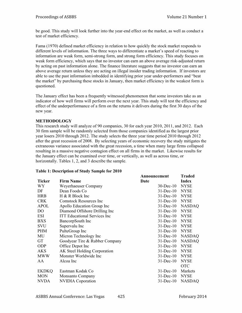
horizontally. Tables 1, 2, and 3 describe the sample.
Table 1: Description of Study Sample for 2010
Ticker Firm Name
Announcement
Date
Traded
Index
WY Weyerhaeuser Company 30-Dec-10 NYSE
DF Dean Foods Co 31-Dec-10 NYSE
HRB H & R Block Inc 31-Dec-10 NYSE
CRK Comstock Resources Inc 31-Dec-10 NYSE
APOL Apollo Education Group Inc 31-Dec-10 NASDAQ
DO Diamond Offshore Drilling Inc 31-Dec-10 NYSE
ESI ITT Educational Services Inc 31-Dec-10 NYSE
BXS BancorpSouth Inc 31-Dec-10 NYSE
SVU Supervalu Inc 31-Dec-10 NYSE
PHM PulteGroup Inc 31-Dec-10 NYSE
MU Micron Technology Inc 31-Dec-10 NASDAQ
GT Goodyear Tire & Rubber Company 31-Dec-10 NASDAQ
ODP Office Depot Inc 31-Dec-10 NYSE
AKS AK Steel Holding Corporation 31-Dec-10 NYSE
MWW Monster Worldwide Inc 31-Dec-10 NYSE
AA Alcoa Inc 31-Dec-10 NYSE
EKDKQ Eastman Kodak Co 31-Dec-10
OTC
Markets
MON Monsanto Company 31-Dec-10 NYSE
NVDA NVIDIA Coporation 31-Dec-10 NASDAQ

Proceedings of ASBBS Volume 21 Number 1
ASBBS Annual Conference: Las Vegas 426 February 2014
WDC Western Digital Corporation 31-Dec-10 NASDAQ
YRCW YRC Worldwide Inc 31-Dec-10 NASDAQ
AIG American International Group Inc 31-Dec-10 NYSE
IPG The Interpublic Group of Companies Inc 31-Dec-10 NYSE
SANM Sanmina Corporation 31-Dec-10 NASDAQ
C Citigroup Inc 31-Dec-10 NYSE
GCI Gannett Co Inc 31-Dec-10 NYSE
AAMRQ AMR Corporation 31-Dec-10
OTC
Markets
WNR Western Refining Inc 31-Dec-10 NYSE
AES The AES Corporation 31-Dec-10 NYSE
THC Tenet Healthcare Corp 31-Dec-10 NYSE
Table 2: Description of Study Sample for 2011
Ticker Firm Name
Announcement
Date
Traded
Index
CYH Community Health Systems Inc 30-Dec-11 NYSE
NIHD NII Holdings Inc 30-Dec-11 NASDAQ
ODP Office Depot Inc 30-Dec-11 NYSE
BAC Bank of America Corporation 30-Dec-11 NYSE
JNS Janus Capital Group Inc 30-Dec-11 NYSE
MTOR Meritor Inc 30-Dec-11 NYSE
RSH RadioShack Corp 30-Dec-11 NYSE
SPLS Staples Inc 30-Dec-11 NASDAQ
AAMRQ AMR Corporation 30-Dec-11
OTC
Markets
YRCW YRC Worldwide Inc 30-Dec-11 NASDAQ
AKAM Akamai Technologies Inc 30-Dec-11 NASDAQ
CSC Computer Sciences Corporation 30-Dec-11 NYSE
SHLD Sears Holding Corporation 30-Dec-11 NASDAQ
X United States Steel Corp 30-Dec-11 NYSE
CVC Cablevision Systems Corporation 30-Dec-11 NYSE
AIG American International Group Inc 30-Dec-11 NYSE
NFLX Netflix Inc 30-Dec-11 NASDAQ
ANR Alpha Natural Resources Inc 30-Dec-11 NYSE
FSLR First Solar Inc 30-Dec-11 NASDAQ
MWW Monster Worldwide Inc 30-Dec-11 NYSE
HCBK Hudson City Bancorp Inc 30-Dec-11 NASDAQ
HSP Hospira Inc 30-Dec-11 NYSE
WHR Whirpool Corp 30-Dec-11 NYSE
FCX Freeport-McMoRan & Gold Inc 30-Dec-11 NYSE
OI Owens-Illinois Inc 30-Dec-11 NYSE
HIG The Hartford Financial Services Group Inc 30-Dec-11 NYSE
HPQ Hewlett-Packard Company 30-Dec-11 NYSE
CMA Comerica Incorporated 30-Dec-11 NYSE
TLAB Tellabs Inc 30-Dec-11 NASDAQ
FHN First Horizon National Corporation 30-Dec-11 NYSE

Proceedings of ASBBS Volume 21 Number 1
ASBBS Annual Conference: Las Vegas 427 February 2014
Table 3: Description of Study Sample for 2012
Ticker Firm Name Announcement Date Traded Index
EXC Exelon Corporation 31-Dec-12 NYSE
RRD R.R. Donnelley & Sons Company 31-Dec-12 NASDAQ
ATI Allegheny Technologies Inc 31-Dec-12 NYSE
PBI Pitney Bowes Inc 31-Dec-12 NYSE
HPQ Hewlett-Packard Company 31-Dec-12 NYSE
JCP J.C. Penney Company Inc 31-Dec-12 NYSE
BBY Best Buy Co Inc 31-Dec-12 NYSE
CLF Cliffs Natural Resources Inc 31-Dec-12 NYSE
AMD Advanced Micro Devices Inc 31-Dec-12 NYSE
APOL Apollo Education Group Inc 31-Dec-12 NASDAQ
ETR Entergy Corporation 31-Dec-12 NYSE
GT Goodyear Tire & Rubber Company 31-Dec-12 NASDAQ
FTR Frontier Communications Corporation 31-Dec-12 NASDAQ
IGT International Game Technology 31-Dec-12 NYSE
SVU Supervalu Inc 31-Dec-12 NYSE
DMND Diamond Foods Inc 31-Dec-12 NASDAQ
KWK Quicksilver Resources Inc 31-Dec-12 NYSE
NAV Navistar International Corporation 31-Dec-12 NYSE
AKS AK Steel Holding Corporation 31-Dec-12 NYSE
ESI ITT Educational Services Inc 31-Dec-12 NYSE
ANR Alpha Natural Resources Inc 31-Dec-12 NYSE
EKDKQ Eastman Kodak Co 31-Dec-12 OTC Markets
NIHD NII Holdings Inc 31-Dec-12 NASDAQ
HD The Home Depot Inc 31-Dec-12 NYSE
MCD McDonald's Corp 31-Dec-12 NYSE
TRV The Travelers Companies Inc 31-Dec-12 NYSE
NCIT NCI Inc 31-Dec-12 NASDAQ
CECO Career Education Corp 31-Dec-12 NASDAQ
GTAT GT Advances Technologies Inc 31-Dec-12 NASDAQ
STI SunTrust Banks Inc 31-Dec-12 NYSE
This study will use the standard risk-adjusted event study methodology from the finance
literature. To test weak form market efficiency the following null and alternative hypothesis will
be used:
H10: The risk adjusted return of the stock price of each annual sample and the global
sample of worst performing firms is not significantly affected by this type of information on the
event day.
H11: The risk adjusted return of the stock price of each annual sample and the global
sample of worst performing firms is significantly negatively affected by this type of information
on the event day.
H20: The risk adjusted return of the stock price of each annual sample and the global
sample of worst performing firms is not significantly affected by this type of information around
the event day as defined by the event period.

Proceedings of ASBBS Volume 21 Number 1
ASBBS Annual Conference: Las Vegas 428 February 2014
H21: The risk adjusted return of the stock price of each annual sample and the global
sample of worst performing firms is significantly affected by this type of information around the
event day as defined by the event period.
The Data for this study will be collected from http://finance.yahoo.com/. The event date (Day 0)
is the last trading day for the tax calendar year. Every stock return from the companies and from
the S&P 500 index will also be collected from http://finance.yahoo.com/.
The event study methodology follows:
1. Historical prices for both the firms and the S&P 500 will be collected from day -180 to
day +30, being the event period -30 to +30 and Day 0 the announcement day.
2. Holding Period Return will be calculated for all the companies as well as for the S&P
500 on the event period days (-180 to +30). HPR will be obtained from the following formula:
Current Daily Return = (current day close price – previous day close price) / prev. Day close price
3. A regression analysis was be performed with firm return as the dependent variable and
the corresponding S&P return as the independent variable over the pre-event period (from day -
180 to -30). The alphas and the betas were obtained from the regression. 90 regressions were
performed.
Table 4: Alphas and Betas of Study Sample
2010
Company Alpha Beta
WY 0.000356162 1.345358787
DF -0.004538366 0.358301265
HRB -0.001836898 0.944571163
CRK -0.001969006 1.352763616
APOL -0.003324069 0.560923574
DO -0.001273077 1.043600818
ESI -0.003413117 0.594246121
BXS -0.002965725 1.0149153
SVU -0.003085672 1.197011085
PHM -0.002815007 1.597856726
MU -0.002234814 1.869010551
GT -0.002085738 1.768407324
ODP -0.002949085 2.207353505
AKS -0.002788258 1.778870431
MWW 0.002030169 1.8942236
AA -0.000197848 1.444333238
EKDKQ -0.002100564 1.938079457
MON -0.00026822 0.777766267
NVDA -0.001592304 1.33417143
WDC -0.001386812 1.332350802
YRCW -0.005050456 1.504280592
AIG 0.000881022 1.58873504
IPG 0.001370536 1.608747079
SANM -0.002367177 2.254301719
C -0.000488029 1.380144293
GCI -0.001860449 1.743739833
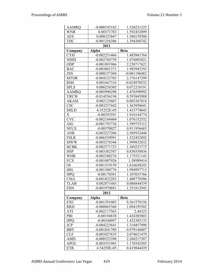
Proceedings of ASBBS Volume 21 Number 1
ASBBS Annual Conference: Las Vegas 429 February 2014
AAMRQ -0.000192182 1.520231325
WNR 0.00371783 1.592452899
AES 0.000323847 1.560159386
THC -0.001256386 1.394360742
2011
Company Alpha Beta
CYH -0.002251466 1.485841764
NIHD -0.002784759 1.076003821
ODP -0.001891966 2.238717621
BAC -0.003881371 1.985945393
JNS -0.000157304 -0.081196482
MTOR -0.004323765 2.376147299
RSH 0.001667316 -0.024970532
SPLS 0.000258305 0.072210191
AAMRQ -0.005996298 1.476590992
YRCW -0.014556194 0.593845988
AKAM 0.002125607 0.003367818
CSC -0.003237442 1.363958641
SHLD 4.35252E-05 1.415774643
X -0.00293591 1.918144774
CVC -0.002184404 1.076152532
AIG -0.001793736 1.599753312
NFLX -0.00570027 0.911956683
ANR -0.003227206 2.505932448
FSLR -0.006539991 1.522452892
MWW -0.003278344 1.999832832
HCBK -0.002571723 1.369253775
HSP -0.003382587 0.830350836
WHR -0.002388276 1.175521143
FCX -0.001007926 1.58989414
OI -0.001519159 1.616630243
HIG -0.001380776 1.994997713
HPQ -0.00176581 1.107653766
CMA -0.001822283 1.408770506
TLAB 0.002871443 0.086844539
FHN -0.001970881 1.551812945
2012
Company Alpha Beta
EXC -0.001391083 0.361570156
RRD -0.000865368 1.094195502
ATI -0.002117563 2.44323
PBI -0.00194838 1.424385803
HPQ -0.00344097 1.432385135
JCP -0.004223641 1.310457998
BBY -0.001841789 0.979146807
CLF -0.003427635 2.074621479
AMD -0.008523398 2.268217587
APOL -0.003551985 1.178542505
ETR 4.54258E-05 0.419844439

Proceedings of ASBBS Volume 21 Number 1
ASBBS Annual Conference: Las Vegas 430 February 2014
GT 0.000763955 1.767670988
FTR 0.00102147 0.518589425
IGT -0.001164115 1.269336899
SVU -0.003520541 1.457361474
DMND -0.001628047 0.672376421
KWK -0.001809556 2.324921577
NAV -0.003032515 2.732759676
AKS -0.003520873 2.286965483
CLF -0.003427635 2.074621479
ANR -0.003437107 2.661229407
EKDKQ 0.001109714 0.869217378
NIHD -0.007366774 1.124747759
HD 0.001572561 0.919610609
MCD -0.00088545 0.566082088
TRV 0.001245791 0.77373781
NCIT -0.000932024 0.12477702
CECO -0.005081206 1.750229582
GTAT -0.004511232 2.202288234
STI 0.000964335 1.577049028
4. The expected return for each firm wil be calculated:
Expected Return = Alpha + Beta x S&P actual return
5. Excess Return will be obtained from the difference between Actual and Expected
Return. Excess Return = Actual Return – Expected Return.
6. Average Excess Return (for the Event period) will be calculated as:
Average Excess Return (AER) = Total Excess Return / n (number of firms in the sample).
7. Cumulative Average Excess Return for the event period (Day -30 to Day +30) will be
calculated by adding the AER for each day in the event period.
8. A graph of AER and Cumulative AER, plotted for the event period (days -30 to +30),
will accompany the data and research.
This analysis will graph the trends of the stock return variation over the event period. The
research will determine the significance and timing of the reaction in the stock return of the worst
performing firms over the event period.
QUANTITATIVE TESTS AND RESULTS
Is the market weak form efficient? If it is, how is the stock market affected by a trading strategy
based on past information such as selling of stock losers at year end and buying the same in
January? This study will observe and compare the average actual return as well as the average
expected return. If the January effect surfaces, it would not be surprising to observe a difference
between the average actual return and the average expected return over the event period (from
day -30 to day + 30). To statistically test for a difference in the Actual Daily Average Returns (for
the firms over the time periods day -30 to day +30) and the Expected Daily Average Returns (for
the firms over the time periods day -30 to day +30), we conducted a paired sample t-test and
found a significant difference at the 5% level between actual average daily returns and the risk
adjusted expected average daily returns for the year 2010, but no significant difference for the
years 2011 and 2012. Results here support the null hypothesis H20: The risk adjusted return of the
stock price of each annual sample and the global sample of worst performing firms is not
significantly affected by this type of information around the event day as defined by the event

Proceedings of ASBBS Volume 21 Number 1
ASBBS Annual Conference: Las Vegas 431 February 2014
period. This finding fails to support the significance of the information around the event since the market’s reaction was not observed.
Another purpose of this analysis was to test the efficiency of the market in reacting to year end selling and repurchasing in January. Specifically, do we observe weak form market efficiency as defined by Fama, 1970, in the efficient market hypothesis? The key in the analysis or tests is to determine if the AER (Average Excess Return) and CAER (Cumulative Average Excess Return) are significantly different from zero or that there is a visible graphical or statistical relationship between time and either AER or CAER. See AER and CAER graphs in Charts 1 through 6 below. CHART 1: AVERAGE EXCESS RETURN FOR YEAR 2010
CHART 2: CUMULATIVE AVERAGE EXCESS RETURN FOR YEAR 2010
The graph in chart 2 shows that January effect had a positive impact on stock price beginning 21
days before the announcement day 0, the last trading day of the year and continued to make a
positive impact on stock price until day 5. This evidence supports the null hypothesis H10: The
risk adjusted return of the stock price of each annual sample and the global sample of worst
-0.02
-0.015
-0.01
-0.005
0
0.005
0.01
0.015
0.02
-30
-27
-24
-21
-18
-15
-12 -9 -6 -3 0 3 6 9
12
15
18
21
24
27
30A
ER
TIME
TIME vs AER
AER
-0.02
0
0.02
0.04
0.06
0.08
0.1
0.12
0.14
-30
-27
-24
-21
-18
-15
-12 -9 -6 -3 0 3 6 9
12
15
18
21
24
27
30
CA
ER
TIME
TIME VS CAER
CAER
Proceedings of ASBBS Volume 21 Number 1
ASBBS Annual Conference: Las Vegas 432 February 2014
performing firms is not significantly affected by this type of information on the event day. For the
sample of firms analyzed, price does not significantly drop on the event day, instead stock price
began to rise up to 21 days before the event day.
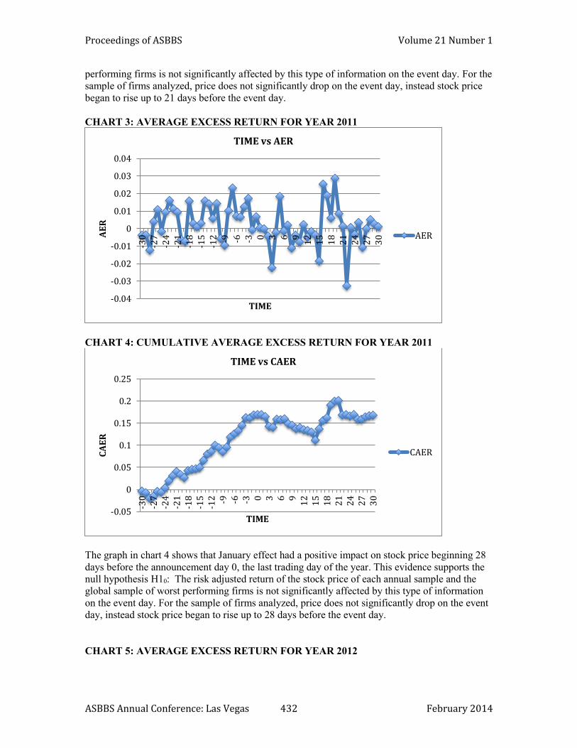
CHART 3: AVERAGE EXCESS RETURN FOR YEAR 2011
CHART 4: CUMULATIVE AVERAGE EXCESS RETURN FOR YEAR 2011
The graph in chart 4 shows that January effect had a positive impact on stock price beginning 28
days before the announcement day 0, the last trading day of the year. This evidence supports the
null hypothesis H10: The risk adjusted return of the stock price of each annual sample and the
global sample of worst performing firms is not significantly affected by this type of information
on the event day. For the sample of firms analyzed, price does not significantly drop on the event
day, instead stock price began to rise up to 28 days before the event day.
CHART 5: AVERAGE EXCESS RETURN FOR YEAR 2012
-0.04
-0.03
-0.02
-0.01
0
0.01
0.02
0.03
0.04
-30
-27
-24
-21
-18
-15
-12 -9 -6 -3 0 3 6 9
12
15
18
21
24
27
30A
ER
TIME
TIME vs AER
AER
-0.05
0
0.05
0.1
0.15
0.2
0.25
-30
-27
-24
-21
-18
-15
-12 -9 -6 -3 0 3 6 9
12
15
18
21
24
27
30
CA
ER
TIME
TIME vs CAER
CAER

Proceedings of ASBBS Volume 21 Number 1
ASBBS Annual Conference: Las Vegas 433 February 2014
CHART 6: CUMULATIVE AVERAGE EXCESS RETURN FOR YEAR 2012
The graph in chart shows that January effect had a positive impact on stock price beginning 30
days before the announcement day 0, the last trading day of the year and continued to make a
positive impact until day 25. This evidence supports the null hypothesis H10: The risk adjusted
return of the stock price of each annual sample and the global sample of worst performing firms
is not significantly affected by this type of information on the event day. For the sample of firms
analyzed, price does not significantly drop on the event day, instead stock price began to rise up
to 30 days before the event day. These results are consistent with the weak form market
efficiency hypothesis which states that the stock price reflects all past information.
CONCLUSION This study tested the effect of year end selling of underperforming stocks on the stock price’s risk
adjusted rate of return for a randomly selected sample of 90 firms, 30 from 2010, 30 from 2011,
and 30 from 2012. The standard risk adjusted event study methodology was used. The study
analyzed 18,990 past observations on the ninety publicly traded firms and the S&P 500 market
index. Appropriate statistical tests for significance were conducted. Results failed to show a
-0.03
-0.02
-0.01
0
0.01
0.02
0.03
-30
-27
-24
-21
-18
-15
-12 -9 -6 -3 0 3 6 9
12
15
18
21
24
27
30A
ER
TIME
TIME vs AER
AER
-0.05
0
0.05
0.1
0.15
0.2
-30
-27
-24
-21
-18
-15
-12 -9 -6 -3 0 3 6 9
12
15
18
21
24
27
30
CA
ER
TIME
TIME vs CAER
CAER

Proceedings of ASBBS Volume 21 Number 1
ASBBS Annual Conference: Las Vegas 434 February 2014
negative market reaction prior to the event day, the last trading day of the year. Findings also
support efficient market theory at the weak form level as documented by Fama (1970).
Specifically, for this study selling up until the event day was not found, instead stock prices
increased beginning 21 to 30 days prior to the last trading day of the year. This study suggests
that the market is efficient with respect to the January effect. Results here also support weak form
market efficiency.
REFERENCES
Fama, E. (1970). Efficient capital markets: A review of theory and empirical work. The journal of
finance, 25(2), 383-417. Retrieved from http://www.jstor.org/stable/2325486
Haugen, R. A., & Lakonishok, J. (1988). The incredible january effect: the stock market's
unsolved mystery. Homewood, Illinois: Dow Jones-Irwin.
Haugen, R. A., & Jorion, P. (1996). The january effect: Still there after all these years. Financial
Analysts Journal, 52(1), 27-31.
Retrieved from http://www.jstor.org/stable/4479893
Haug, M., & Hirschey, M. (2006). The january effect.Financial Analysts Journal, 62(5), 78-88.
Retrieved from http://www.jstor.org/discover/10.2307/4480774
Keim, D. (1983). Size-related anomalies and stock return seasonality: Further empirical
evidence. Journal of Financial Economics, Retrieved from
http://www.buec.udel.edu/coughenj/finc872_keim_jfe1983.pdf
Reinganum, M. R. (1983). The anomalous stock market behavior of small firms in
january: Empirical tests for tax-loss selling effects. Journal of Financial
Economics, 12(1), 89-104.
Ritter, J. R. (1988). The buying and selling behavior of individual investors at the turn of the
year. Journal of Finance, 43(3), 701-717.
Rozeff, M. S., & Kinney Jr., W. R. (1976). Capital market seasonality: The case of stock
returns. Journal of Financial Economics, 3(4), 379-402.
Wachtel, S. B. (1942). Certain observations on seasonal movements in stock prices. The journal
of business of the University of Chicago, 15(2), 184-193.
Retrieved from http://www.jstor.org/stable/2350013