The Ionosphereindico.ictp.it/event/a11159/session/65/contribution/42/material/0/... · Jamming....

2333-25

Workshop on Science Applications of GNSS in Developing Countries (11-27 April), followed by the: Seminar on Development and Use of the Ionospheric

NeQuick Model (30 April-1 May)

RADICELLA Sandro Maria

11 April - 1 May, 2012

Abdus Salam International Centre For Theoretical Physics Telecommunications ICT for Development Laboratory

(T/ICT4D),Via Beirut 7 Trieste ITALY

The Ionosphere

The Ionosphere

Sandro M. Radicella Telecommunica+ons/ICT for Development Laboratory

the Abdus Salam ICTP, Trieste, Italy

Workshop on Science Applications of GNSS in Developing Countries

(11-27 April 2012)

This lecture

•  The importance of the Ionosphere for systems depending on radio signals

•  The atmospheric system

•  Forma;on of the ionosphere

•  Ionospheric structure •  Ionospheric varia;ons

The importance of the Ionosphere for systems depending on radio

signals

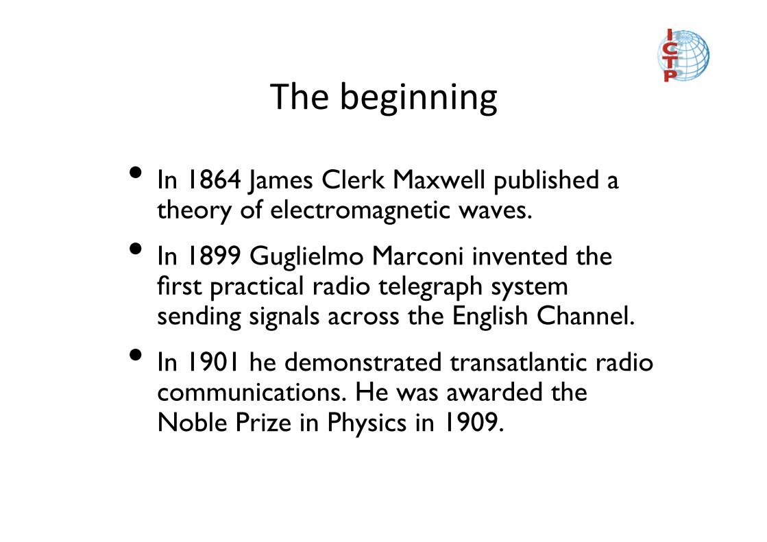
The beginning

•  In 1864 James Clerk Maxwell published a theory of electromagnetic waves.

•  In 1899 Guglielmo Marconi invented the first practical radio telegraph system sending signals across the English Channel.

•  In 1901 he demonstrated transatlantic radio communications. He was awarded the Noble Prize in Physics in 1909.

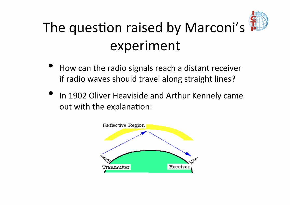
The ques8on raised by Marconi’s experiment

•  How can the radio signals reach a distant receiver if radio waves should travel along straight lines?

•  In 1902 Oliver Heaviside and Arthur Kennely came out with the explana8on:

Implica8ons to the radio communica8ons (1)

For the most of the 20 century radio communica;ons relied on HF frequencies (3-‐30 MHz) that used the ionosphere as reflector.

The applica;ons included:

•  Radio Broadcas;ng •  Civilian point-‐to-‐point communica;ons

•  Military communica;ons and surveillance

•  Ship-‐to-‐shore communica;ons

•  Trans-‐oceanic aircraJ links •  Jamming

Implica8ons to the radio communica8ons (2)

In the 21 century:

The applica;ons are mostly related to trans-‐ionospheric radio links including civilian and military satellite communica;ons and satellite naviga;on systems.

The atmospheric system

The study of the atmospheric system: a word of warning

•  The atmospheric system is not normally studied as a system but taking only into account one par;cular element of the system as its temperature or ioniza;on.

•  This approach reduces the possibili+es of a full understanding of the atmospheric system behavior as a whole.

Atmospheric structure: temperature

The termal structure is described as a number of layers (-‐spheres) separated by -‐pauses which are defined as the inflec8on points in the temperature profile. As an example: the tropopause defines the top of the troposphere where the temperature gradient turns over from nega8ve to posi8ve.

Why this thermal structure ?

•  The troposphere is heated mainly by the ground, which absorbs solar radia;on and re-‐emits it in the infra-‐red.

•  The stratosphere above the troposphere has a posi;ve temperature gradient due to hea;ng from the ozone which absorbs the solar ultra-‐violet radia;on that penetrates down to these al;tudes.

•  In the mesosphere, above 50 km, the density of ozone drops off faster than the increase in incoming radia;on can compensate for and the temperature decreases with al;tude.

•  The thermosphere is heated mainly by absorp;on of EUV and XUV radia;on through dissocia;on of molecular oxygen.

Atmospheric composi8on: ground level

•  By mass

•  Nitrogen: ~ 76%

•  Oxygen: ~ 23 %

•  Argon: ~ 1%

•  By volume

•  Nitrogen: ~78%

•  Oxygen: ~21%

•  Argon: ~1%

Atmospheric composi8on as a func8on of height

Mixing and molecular diffusion:

•  Turbulent mixing: lower and middle atmosphere

•  Does not depend on molecular weight.

•  Composi;on tends to be independent of height

•  Diffusion: upper atmosphere

•  Mean molecular weight of mixture gradually decreases with height.

•  Only lightest gases are present at higher levels.

•  Each gas behaves as if it were alone.

•  Density drops-‐of exponen+ally with height Near 100km: diffusion = turbulent mixing.

A closer look to the atmospheric pressure

Neutral atmosphere composi8on in the upper atmosphere

Atmospheric Hydrosta8c Equilibrium

Scale Height

In various scien;fic contexts, a “Scale Height” is a distance over which a quan;ty decreases by a factor of e.

The “scale height” defined in the previous slide is the “pressure scale height” that, considering the perfect gas law and the troposphere composed mostly by N2 (m=2 x 14 x 1.66x10-27 kg):

m = 4.65x10-26 kg g = 9.8 m/s2 and T ~ 300 K, we get:

H = 9x103 m = 9 km

Forma8on of the ionosphere

Photochemical processes in the atmosphere

•  The atmosphere of the Earth is made up of a large number of chemical cons;tuents.

•  We have seen that the most abundant or major cons;tuents are N2, O2 and Ar, but many more cons;tuents are produced in the atmosphere itself by photochemical processes or at the surface by different natural processes and human ac;vity.

•  Photochemical processes play a fundamental role in the middle and upper atmosphere including the ionosphere.

Main photochemical absorp8on processes of solar radia8on

Solar radia8on penetra8on heights

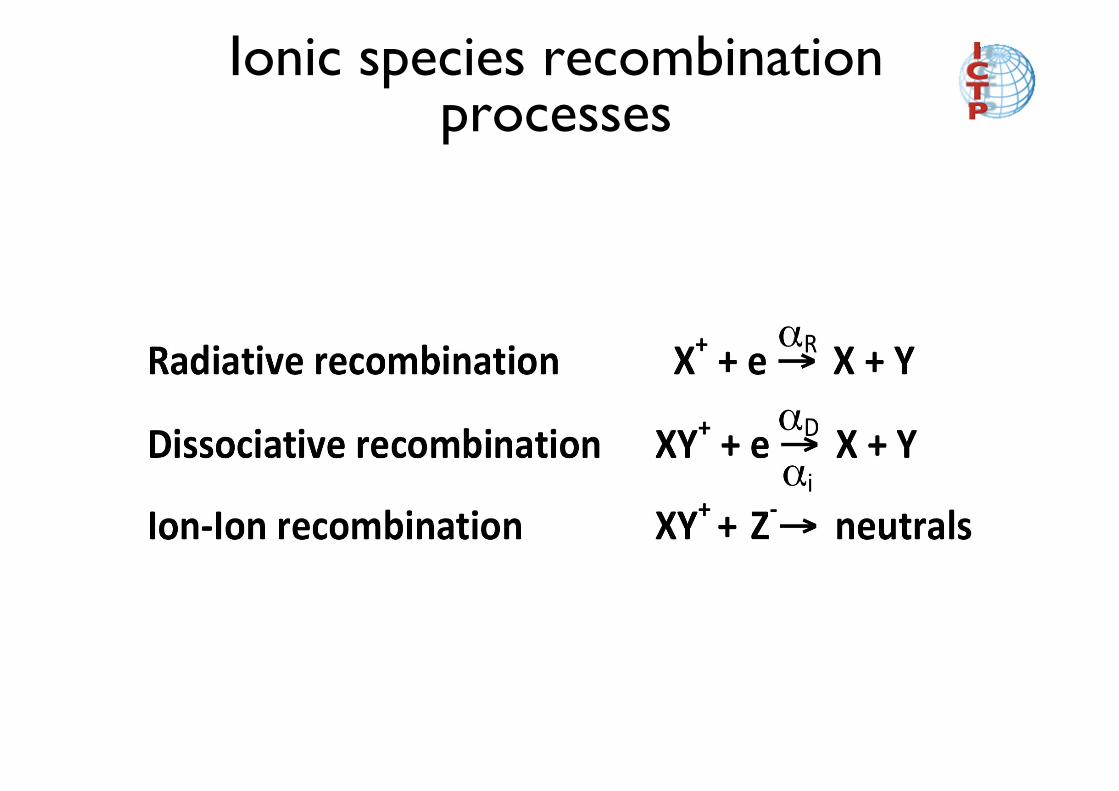
Ionic species recombination ��processes

Forma8on of the Ionosphere

Solar UV and X radiation impinges at angle χν,

It is absorbed in the upper atmosphere and ionizes the neutral atmosphere

I∞ is the flux on top of the layer.

Basic equa8ons of solar radia8on absorp8on in the atmosphere (1)

H is the scale height,

H= kBTn/mng,

with g being the gravitational acceleration at height z = 0, where the density is n0.

According to radiative transfer theory, the incident solar radiation diminishes with altitude along the ray path in the atmosphere.

σν is the radiation absorption cross section for radiation (photon) of frequency ν.


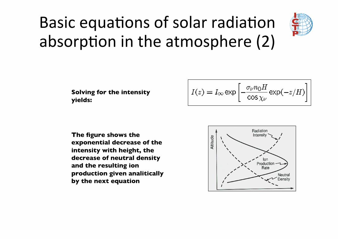
Solving for the intensity yields:

The figure shows the exponential decrease of the intensity with height, the decrease of neutral density and the resulting ion production given analitically by the next equation


The number of electron-ion pairs locally produced by the solar radiation, the photoionization rate per unit volume qν(z), is proportional to the ionization efficiency, κν , and absorbed radiation: qν(z) = κν σνnnI(z).

This equation describes the formation of the Chapman layer and represents the basis of the theory of the photochemical processes in the atmosphere.


Recombination, with coefficient αr, and electron attachment, βr, are the two major loss processes of electrons in the ionosphere.

In equilibrium quasi-neutrality applies:

ne = ni

Then the continuity equation for ne reads:

Chapman layer theory

A theore+cal distribu+on of ioniza+on as a func+on of height produced solely by the absorp+on of solar radia+on by a single atmospheric cons+tuent.

Named for Sydney Chapman, who first derived the shape of such a distribu;on mathema;cally.

Some of the basic assump;ons used to develop the equa;on were that

•  The ionizing radia+on from the sun is monocroma+c,

•  The single neutral cons+tuent to be ionized is distributed exponen+ally (i.e., with a constant scale height),

•  There is equilibrium between the crea+on of free electrons and their loss by recombina+on.

Ionospheric structure

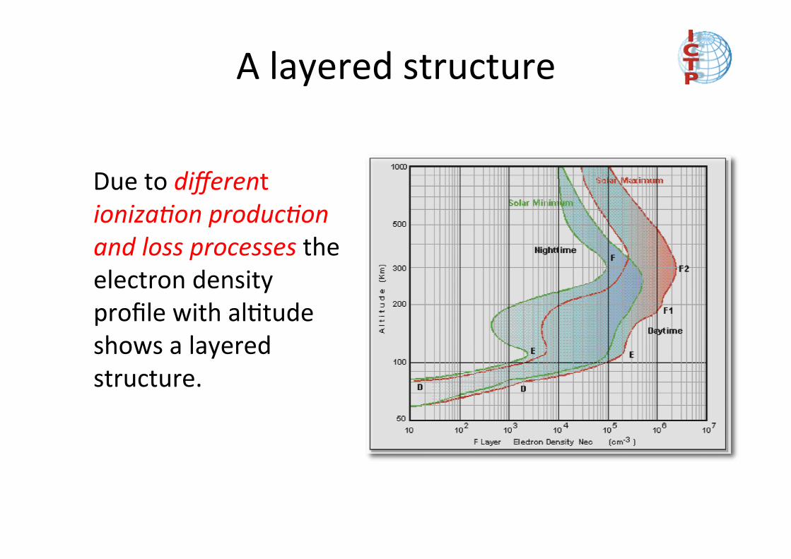
A layered structure

Due to different ioniza4on produc4on and loss processes the electron density profile with al8tude shows a layered structure.

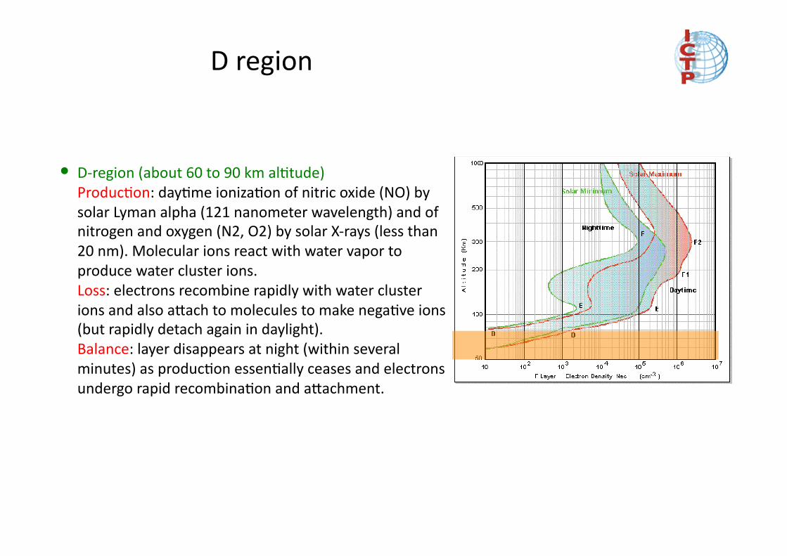
D region

•  D-‐region (about 60 to 90 km al8tude) Produc8on: day8me ioniza8on of nitric oxide (NO) by solar Lyman alpha (121 nanometer wavelength) and of nitrogen and oxygen (N2, O2) by solar X-‐rays (less than 20 nm). Molecular ions react with water vapor to produce water cluster ions. Loss: electrons recombine rapidly with water cluster ions and also abach to molecules to make nega8ve ions (but rapidly detach again in daylight). Balance: layer disappears at night (within several minutes) as produc8on essen8ally ceases and electrons undergo rapid recombina8on and abachment.

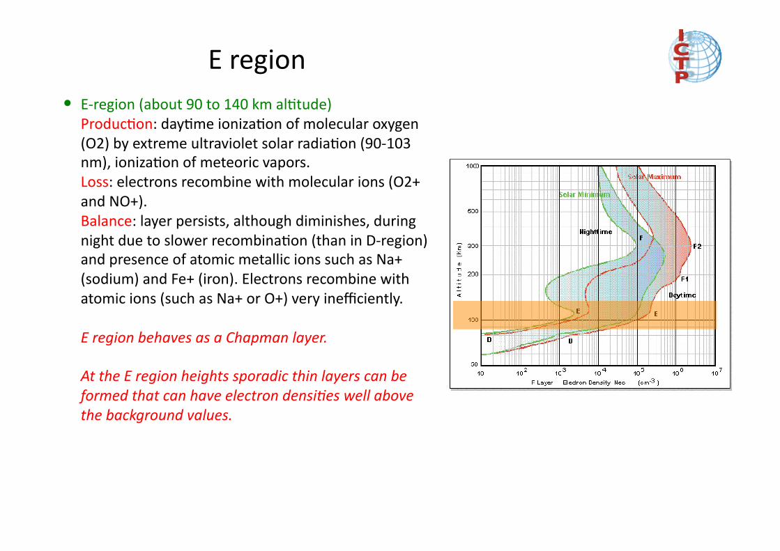
E region •  E-‐region (about 90 to 140 km al8tude) Produc8on: day8me ioniza8on of molecular oxygen (O2) by extreme ultraviolet solar radia8on (90-‐103 nm), ioniza8on of meteoric vapors. Loss: electrons recombine with molecular ions (O2+ and NO+). Balance: layer persists, although diminishes, during night due to slower recombina8on (than in D-‐region) and presence of atomic metallic ions such as Na+ (sodium) and Fe+ (iron). Electrons recombine with atomic ions (such as Na+ or O+) very inefficiently.

E region behaves as a Chapman layer.

At the E region heights sporadic thin layers can be formed that can have electron densi4es well above the background values.

F region

•  F-‐region (above 140 km al8tude) Produc8on: day8me ioniza8on of atomic O by extreme ultraviolet (EUV) solar radia8on (20 -‐ 90 nm). O+ converted to NO+ by molecular nitrogen (N2)

•  F1-‐layer (about 140 to 200 km al8tude) Loss: controlled by recombina8on of NO+ ions with electrons. Balance: layer diminishes at night as electrons recombine with NO+.

F1 layer behaves as a Chapman layer

F1 layer

•  F2-‐layer (peak about 300 to 400 km al8tude) Loss: controlled by O+ reac8on with molecular nitrogen (N2), electrons recombine quickly with ion product (NO+) as it is created. Balance: layer persists through night (becoming simply the F-‐region) since the small supply of N2 leads to slow conversion of O+ to NO+ and hence only a small reduc8on in the number of electron.

Transport processes become important in the F2 and upper F regions, including ambipolar diffusion and wind-‐induced driEs along B, and

and electrodynamic driEs across B.

F2 layer

F2 region chemistry

The recombination process is two-stage:

O++N2 → NO++N (attachment like) rate ∝β [O+]

- controls the rate at high altitudes

NO++e → N+O rate ∝ α [NO+][Ne]

- controls the rate at low altitudes

Continuity equation and Ion transport in the F region

Ions and electrons, once formed (P), will tend to recombine (L) but they are also affected by transport with a plasma drift V.

Ions and electrons will be influenced by the vertical pressure gradient, and the heavier ions will tend to ‘settle’. But, the resultant separation will form an electric field which will tend to restore the system.

€

∂ne∂t

= P − L − div(neV )

∂ne∂t

= q −βne − div(neV )

F region in summary

•  The lowest region (F1), where photochemistry dominates.

•  The transi8on region from chemical to diffusion(lower F2).

•  The upper region, or topside, where diffusion dominates

•  In the F2, including the topside, the presence of transport processes influenced by the geomagne8c field became important.

Ionospheric varia8ons

Introduc8on to the topic

•  We will concentrate on the regular varia8ons mostly of the F2 layer and in the variability of two parameters that are related to the peak electron density and the electron content in the ionosphere.

•  The star8ng point will be a men8on to the experimental techniques used to derive these parameters

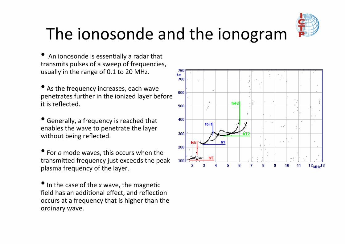
The ionosonde and the ionogram •  An ionosonde is essen8ally a radar that transmits pulses of a sweep of frequencies, usually in the range of 0.1 to 20 MHz.

•  As the frequency increases, each wave penetrates further in the ionized layer before it is reflected.

•  Generally, a frequency is reached that enables the wave to penetrate the layer without being reflected.

•  For o mode waves, this occurs when the transmibed frequency just exceeds the peak plasma frequency of the layer.

•  In the case of the x wave, the magne8c field has an addi8onal effect, and reflec8on occurs at a frequency that is higher than the ordinary wave.

Cri8cal frequencies

The frequency at which a wave just penetrates an ionospheric layer is known as the cri8cal frequency of that layer. The cri8cal frequency is related to the electron density by the simple rela8on:

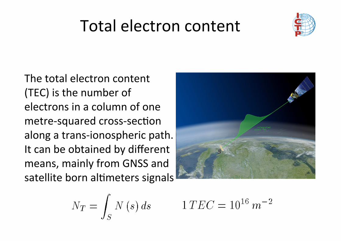
Total electron content

The total electron content (TEC) is the number of electrons in a column of one metre-‐squared cross-‐sec8on along a trans-‐ionospheric path. It can be obtained by different means, mainly from GNSS and satellite born al8meters signals

00

02

04

06

08

10

12

14

16

18

20

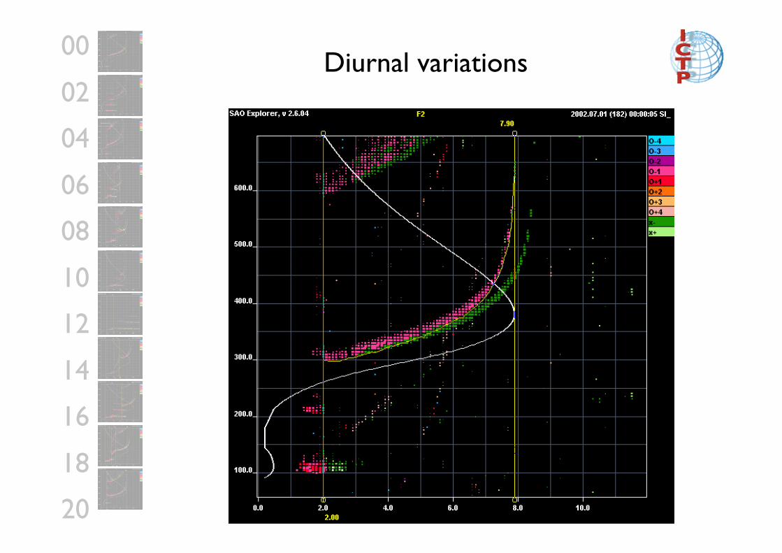
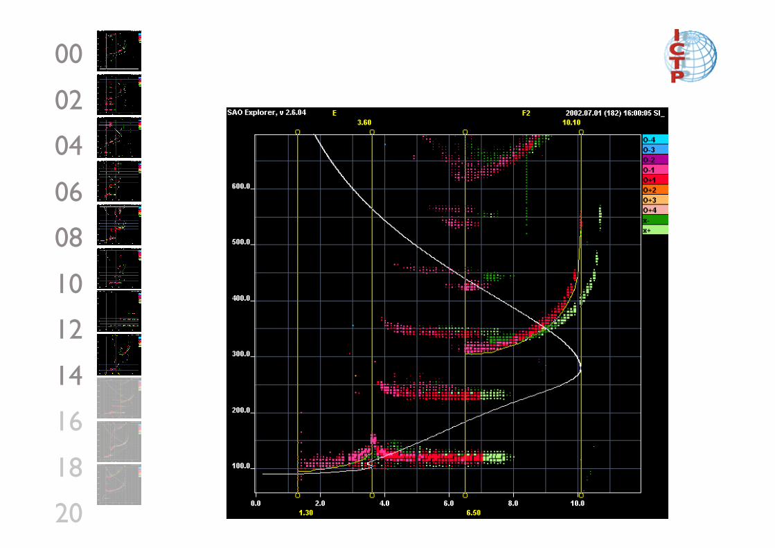
Diurnal variations

00

02

04

06

08

10

12

14

16

18

20

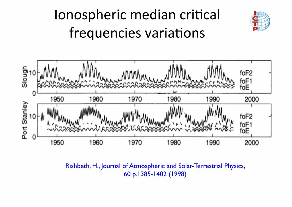
Ionospheric median cri8cal frequencies varia8ons

Rishbeth, H., Journal of Atmospheric and Solar-Terrestrial Physics, 60 p.1385-1402 (1998)

Diurnal and day-‐to-‐day variability of NmF2

Varia;on of NmF2 at Slough for every day during four 2-‐month periods in 1973-‐1974.

H. Rishbeth, M. Mendillo / Journal of Atmospheric and Solar-Terrestrial Physics 63 (2001) 1661–1680

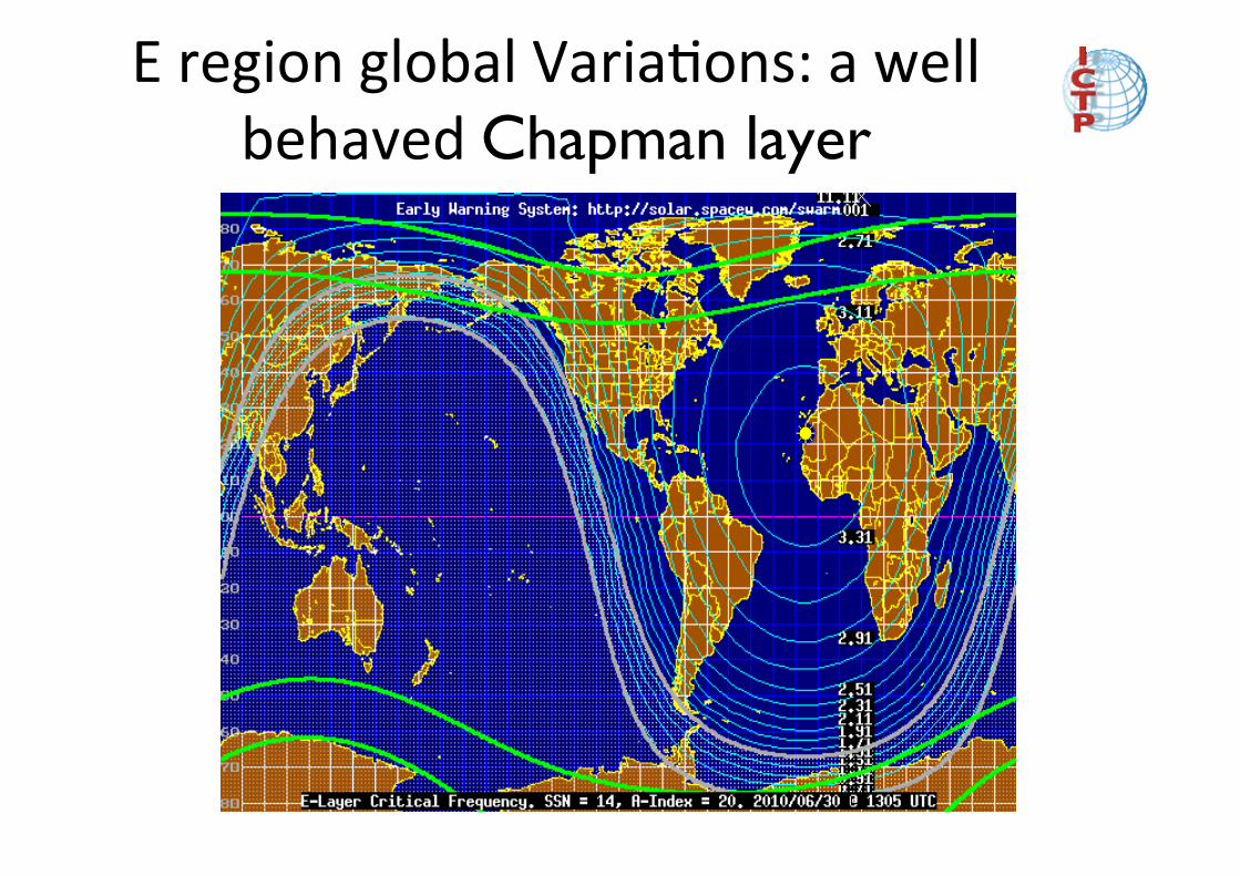
E region global Varia8ons: a well behaved Chapman layer

Global variations of foF2 ��April (R12=100)

Geographical varia8ons: the equatorial anomaly

From the Chapman theory it can be expected that the electron density maximises over the geographic equator at equinox. However, it actually maximises ~ 10-‐20 degrees of geomagne;c la;tude N and S, with a small minima at the equator due to the effect of the geomagne;c field: the ‘fountain effect’.

Nava B., Radicella S.M., Pulinets S. and Depuev V. “Modelling bottom and topside electron density and TEC with profile data from topside ionograms”, Advances in

Space Research, V. 27, pp. 31-34, 2001.

The “fountain effect”

The Equatorial Electrojet drives the F-‐region motor. E-‐field is zonal, magne;c field is meridional, so plasma driJ is ver;cally upwards. Plasma then descends down the magne;c field lines either side of the geomagne;c equator.

Ver8cal TEC diurnal and day-‐to-‐day varia8ons (1)

GPS derived vertical TEC at 5 min interval for Roquetes (Lat. 40.8º, Lon. 0.5º E,Mag. Dip 57º), October 2004

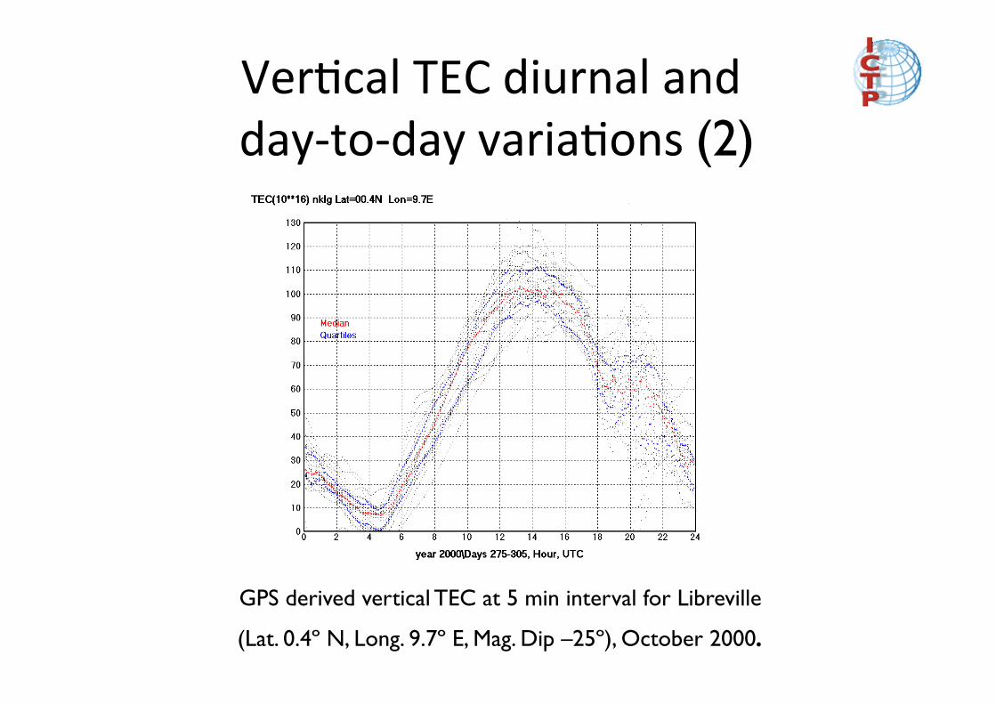
Ver8cal TEC diurnal and day-‐to-‐day varia8ons (2)

GPS derived vertical TEC at 5 min interval for Libreville

(Lat. 0.4º N, Long. 9.7º E, Mag. Dip –25º), October 2000.

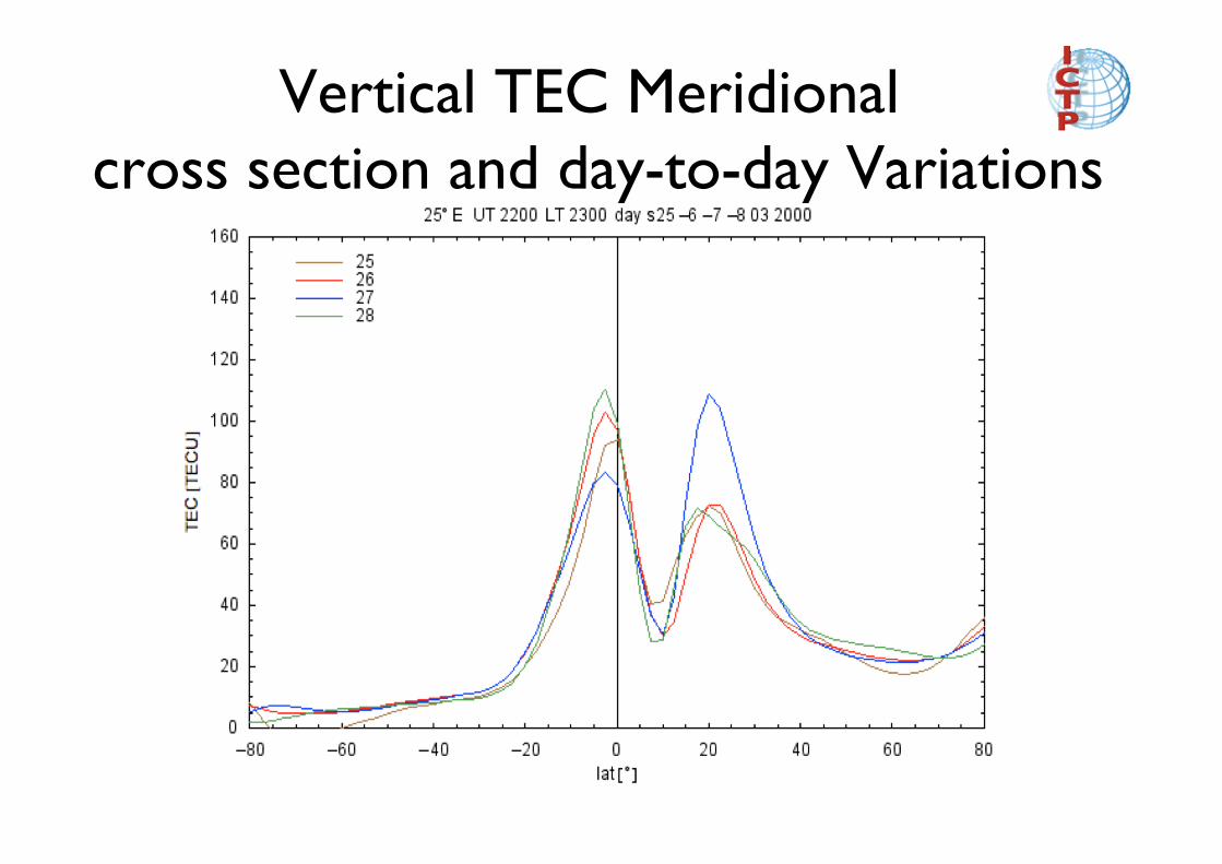
Vertical TEC Meridional ��cross section and day-to-day Variations

Day-‐to-‐day regional TEC ��Variability

Courtesy of P. Doherty and C. Valladares

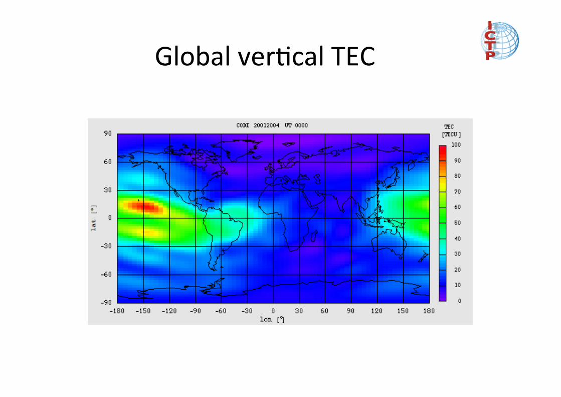
Global ver8cal TEC

This lecture indicates only in a pale way the complexity of the ionosphere but, at the same +me, I hope it awakes more curiosity for this fascina+ng part of our environment.

THANK YOU FOR YOUR ATTENTION!

The Ionosphereindico.ictp.it/event/a11159/session/65/contribution/42/material/0/... · Jamming....

Documents

Transcript of The Ionosphereindico.ictp.it/event/a11159/session/65/contribution/42/material/0/... · Jamming....