The Interplay Between Student Loans and Credit Card

Debt: Implications for Default Behavior∗

Felicia Ionescu

Federal Reserve Board

Marius Ionescu

USNA

February 16, 2015

Abstract

Student loans and credit card loans represent important components of young households’ portfo-

lios in the United States. While default rates on credit card debt are at historically low levels, default

rates on student loans have increased significantly in recent years. There are important institutional

differences between bankruptcy arrangements and default consequences in the two markets, which

may affect default incentives. We theoretically and quantitatively analyze the interactions between

these two forms of unsecured credit and the implications of their financial arrangements for default

behavior of young U.S. households.

We document important facts about the interaction between student loans, credit card debt, and

default on both types of loans and build a general equilibrium model to explain the observed facts. We

theoretically characterize the circumstances under which a household defaults on each of these loans

and demonstrate that the institutional differences between the two credit markets make borrowers

prefer to default on student loans rather than on credit card debt. Our quantitative analysis shows that

the increase in student loan debt during recent years contributed about half of the increase in default

rates, whereas worse labor outcomes for young borrowers during the Great Recession significantly

amplified student loan default. At the same time, the credit card market contraction during this

period helped reduce this effect. An income contingent repayment plan for student loans completely

eliminates the default risk in the credit card market and induces important redistribution effects. This

policy is beneficial (in a welfare improving sense) during the Great Recession, but not during normal

times.

JEL Codes: D91; I22; G19;

Keywords: Default, Bankruptcy, Student Loans, Credit Cards, Great Recession

∗The views expressed herein are those of the authors and do not necessarily reflect those of the Federal ReserveBoard or its staff. The authors thank Simona Hannon, Juan-Carlos Hatchondo, Wenli Li, Leo Martinez, MakotoNakajima, Pierre-Daniel Sarte, Nicole Simpson, and Rob Valletta for comments and participants at the Society forEconomic Dynamics, Midwest Macroeconomics Meeting, Society of Advancements in Economic Theory, the NASM,the NBER, Household Finance group, and seminar participants at Bank of Canada, Colgate University, FRB ofRichmond, Federal Reserve Board, University of Alberta. Special thanks to Kartik Athreya, Satyajit Chatterjee,Dirk Krueger, and Victor Rios-Rull for helpful suggestions and to Gage Love for excellent research assistance.Emails: felicia.ionescu@frb.gov; mionescu@colgate.edu.

1 Introduction

Student loan debt has steadily increased in the last two decades, reaching 1.3 trillion dollars in

2014. In June 2010, total student loan debt surpassed total credit card debt for the first time (see

Figure 10 in Appendix). Currently, 70 percent of individuals who enroll in college take out student

loans; the graduates of 2013 are the most indebted in history, with an average debt load of $27,300

(?). At the same time, the two-year basis cohort default rate (CDR) for Federal student loans

steadily declined from 22.4 percent in 1990 to 4.6 percent in 2005 and has increased ever since,

reaching record highs in the last decade (at 10 percent for FY2011).1 In addition, the majority

of individuals with student loan debt (65 percent) also have credit card debt, according to our

findings from the Survey of Consumer Finances and Equifax. Other surveys and reports also

show that credit card usage is common among college students, with approximately 84 percent

of the student population having at least one credit card in 2008 (?). While both of these loans

represent important components of young households’ portfolios in the United States, the financial

arrangements in the two markets are very different, in particular with respect to the roles played by

bankruptcy arrangements and default pricing. Furthermore, credit terms on credit card accounts

have worsened in recent years, adversely affecting households’ capability to diversify risk but also

limiting the young borrowers’ indebtedness.

We propose a theory about the interactions between student loans and credit card loans in the

United States and their impact on default incentives of young U.S. households. As we argue in this

paper, this interaction between different bankruptcy arrangements induces significant trade-offs in

default incentives in the two markets. Understanding these trade-offs is particularly important in

the light of recent trends in borrowing and default behavior. Data show that young U.S. households

(of which a large percentage have both college and credit card debt) now have the second highest

rate of bankruptcy (just after those aged 35 to 44). Furthermore, the bankruptcy rate among 25-

to 34-year-olds increased between 1991 and 2001, indicating that this generation is more likely to

file for bankruptcy as young adults than were young boomers at the same age.2 Moreover, student

loans have a higher default rate than credit card loans or any other type of loan, including car

loans and home loans.3

These trends are concerning, considering the large risks that young borrowers face: first, the

1The 2-year CDR is computed as the percentage of borrowers who enter repayment in a fiscal year and defaultby the end of the next fiscal year. Trends in the 2-year CDR are presented in Figure 11 in the Appendix.

2Source: www.creditcards.com/.3According to a survey conducted by the FRB New York, the national student loan delinquency rate 60+ days

in 2010 is 10.4 percent compared to only 5.6 percent for the mortgage delinquency rate 90+ days, 1.9 percent forbank card delinquency rate and 1.3 percent for auto loans delinquency rate. Based on an analysis of the PresidentsFY2011 budget, in FY2009 the total defaulted loans outstanding are around $45 billion.

1

college dropout rate has increased significantly in the past decade (from 38 percent to 50 percent

for the cohorts that enrolled in college in 1995 and 2003, respectively). Furthermore, the unem-

ployment rate among young workers with a college education has jumped up significantly during

the Great Recession: 8 percent of young college graduates and 14.1 percent of young workers with

some college education were unemployed in 2010 (Bureau of Labor Statistics). In addition, in or-

der to begin repaying their student loan debt, many college graduates resort to underemployment

outside their fields of study, especially after the Great Recession, a move that may have long-term

deleterious financial effects.4

The combination of high indebtedness and high income risk implies that borrowers are more

likely to default on at least one of their loans. A few questions arise immediately: first, if young

borrowers are constrained in their ability to repay loans, which default option do they find more

attractive and why? In particular, what are the effects of the current financial arrangements in the

two credit markets for default incentives? Second, what are the implications of the interactions

between the two credit markets for student loan and credit card loan policies?

In order to address the proposed issues, we first document facts regarding the interaction

between the two types of credit and default behavior for young borrowers. Using the FRBNY

Consumer Credit Panel (Equifax) data, we find that: 1. young individuals with student loan

debt default at higher rates on their student loans than on their credit card debt; 2. individuals

with credit card debt have higher student loan default rates than individuals without credit card

debt; 3. default on credit card increases in student loan debt; and 4. default on student loans is

hump-shaped in credit card debt.

We next develop a general equilibrium economy that mimics features of student and credit

card loans and explains qualitatively and quantitatively the observed facts on the interaction

between the two markets. Infinitely lived agents differ in student loan debt and income levels.

Agents face uncertainty in income and may save/borrow and, as in practice, borrowing terms are

individual specific. Central to the model is the decision of young college-educated individuals to

repay or default on their credit card and student loans. Consequences of defaulting on student

and credit card loans differ in several important ways: for student loans, they include a wage

garnishment, while for credit card loans, they induce exclusion from borrowing for several periods.

More importantly, credit card loans can be discharged in bankruptcy (under Chapter 7), whereas

student loans cannot be discharged (borrowers need to reorganize and repay under Chapter 13).

Borrowing and default behavior in both markets determine the individual default risk. This risk,

in turn, determines the loan terms agents face on their credit card accounts, including loan prices.

4Research argues that young college-educated individuals graduating during the Great Recession earn 15 to 20percent less on average relative to those who graduated before the Great Recession ?.

2

In contrast, the interest rate in the student loan market does not account for the risk that some

borrowers may default.

In the theoretical part of the paper, we first characterize the default behavior and show how

it varies with households’ characteristics and debt in both markets. Then we demonstrate the

existence of cross-market effects and their implications for default behavior. This represents the

main theoretical contribution of our paper, a contribution which is two-fold:

1) The probability of default on any credit card loan increases with the amount of debt owed in

the student loan market. Also, this default probability is higher for an individual with a default flag

in the student loan market relative to an individual without a default flag. A direct consequence

of this result is that, in equilibrium, credit card loan prices increase in the size of the credit card

loan (as in Chatterjee et al. (2007)), but also increase in the size of the student loan. In addition,

credit card loan prices depend on the default status in the student loan market. To our knowledge,

these results are new in the literature and provide a rationale for pricing credit card loans based

on behavior in all credit markets in which individuals participate.

2) In any steady-state equilibrium, we find combinations of student loan and credit card debt

for which the agent defaults on at least one type of her loans. Moreover, we find that for larger

levels of student loans or credit card debt than the levels in these combinations, default occurs for

student loans. This result implies that while a high student loan debt is necessary to induce default

on student loans, this effect is amplified by indebtedness in the credit card market. This arises

from the differences in bankruptcy arrangements in the two markets: the financially constrained

borrower finds it optimal to default on student loans (even though she cannot discharge her debt)

in order to be able to access the credit card market. Since defaulting on student loans causes

a limited effect on her credit card market participation (shortly-lived exclusion and higher costs

of loans in the credit card market), this borrower prefers the default penalty in the student loan

market over defaulting on her credit card debt, an action which would trigger long-term exclusion

from the credit card market.

In the quantitative part of our paper, we parametrize the model to match statistics regarding

student loan debt, credit card debt, and income of young borrowers with student loans (as delivered

by the SCF 2004-2007). There are several sets of results.

First, our model explains the four main facts described before. Specifically, borrowers with

similar debt levels in the two markets would rather default on student loans than on credit card

debt, and this results in a default rate on student loans in the model of 5 percent and a default

rate on credit card debt of 0.33 percent. Our model is also consistent with the fact that having

debt in the credit card market amplifies the incentive to default on student loans. We find that

individuals with no credit card debt have lower default rates on student loans (4.8 percent) than

3

individuals with credit card debt (5.8 percent). Lastly, our model is consistent with the facts that

default on credit card debt increases in the size of the student loan and that student loan default

presents a hump-shaped profile across levels credit card debt. The first relationship is simply a

consequence of the fact that the individual debt burden, which is the main driver of credit card

default, declines with student loans, which in the model, simply represent an additional per period

payment. The hump-shape profie of student loan default across credit card debt levels is more

interesting because it represents the net effect of several factors. Individuals with medium levels

of student loan debt use credit card debt to reduce their default on student loans. On the one

hand, participating in the credit card market pushes borrowers towards increased default on their

student loans, while on the other hand, taking on credit card debt helps student loan borrowers

smooth consumption and pay their student loan debt, in particular when their student loan debt

burdens are large. At the same time, given the importance of student loan borrowing and default

behavior in credit card loan pricing, individuals with high levels of credit card debt are mostly

“good risk” borrowers, i.e. individuals with low levels of student loan debt. Overall, these three

effects deliver the hump-shaped profile of student loan default on credit card debt. Similarly, our

model delivers a hump-shaped profile of student loan default on income. Individuals with medium

levels of income default the most on their student loan debt but not as frequently on their credit

card debt.

Second, we find large gaps in credit card rates across individuals with different levels of student

loan debt and default status in the student loan market. This result strengthens our theory and

emphasizes the quantitative importance of correctly pricing credit card debt based on behavior in

other credit markets.

Next, we use our theory to explore the policy implications of our model and study the impact of

alternative credit card loan market and student loan arrangements. Specifically, we first run several

experiments in the credit card market in order to quantify the importance of the three channels

that deliver the hump-shaped profile of student loan default. We consider different pricing schemes

for credit card debt, in particular a scheme that does not take into account the borrowing and

repayment behavior in the student loan market, as well as a scheme with tight homogenous limits

on credit card accounts. Second, we consider an income contingent repayment plan on student

loans.5 We find that the income contingent plan completely eliminates the default risk in the credit

card market and induces high levels of dischargeability of student loans. Overall, the policy induces

an increase in welfare of 2.86 percent in an economy with tight credit (similar to the one during the

financial crisis), but has a negative, although small, effect on welfare in the benchmark economy

5The income contingent plan assumes payments of 20 percent of discretionary income and loan forgiveness after25 years. Details are presented in Section 4.4.

4

(0.14 percent).6 The elimination of risk in the crisis environment more than outweighs the welfare

cost associated with high dischargeability and thus with high taxation in the economy. Results

show important redistributional effects: poor borrowers with large levels of student loans benefit

from the policy, while medium income borrowers with low and medium levels of debt are hurt by

it. Medium earners are precisely the group who default the most under the standard repayment

plan. Under income contingent repayment plans, these borrowers repay most of the student loan

debt without discharging and also pay higher taxes to pay for bailing out delinquent borrowers. In

contrast, poor borrowers with large levels of student loans are most likely to discharge their student

loan debt under income contingent repayment plans, whereas in the absence of this repayment plan

they are most likely to discharge their credit card debt. Our findings are particularly important

in the current market conditions in which, due to a significant increase in college costs, students

borrow more than ever in both the student loan and the credit card markets, and at the same

time, they face worse job outcomes and more severe terms on their credit card accounts.

Lastly, we use our model to disentangle the quantitative effects of three potential factors that

contributed to the increase in student loan default during 2007-2010 (from 5 percent to 9 percent).

We find that the accumulation of student loan debt accounts for almost half of the increase in

student loan default and worse income prospects for college students during this period accounts

for the rest. The changes in the credit card market have not contributed to the increase in student

loan default, primarily because of two offseting forces: on the one hand, there has been a decline in

the risk free interest rate, which delivers a decline in default incentives, and, on the other hand, the

credit card market contracted, which delivers an increase in default incentives. We conclude that

the combination of increased student loan debt and lower income represent the main drivers for the

increased default in the student loan market in recent years. At the same time, the developments

in the credit card market during this period helped keep student loan default low.

1.1 Related literature

Our paper is related to two strands of existing literature: credit card debt default and student loans

default. The first strand includes important contributions by Athreya et al. (2009), Chatterjee et al.

(2007), Chatterjee et al. (2010), and Livshits et al. (2007). The first two studies explicitly model a

menu of credit levels and interest rates offered by credit suppliers with the focus on default under

Chapter 7 within the credit card market. Chatterjee et al. (2010) provide a theory that explores

the importance of credit scores for consumer credit based on a limited information environment.

6The crisis environment in the paper supposes worse income outcomes, higher transaction costs in the creditcard market and a lower risk-free rate in the economy.

5

Livshits et al. (2007) quantitatively compare liquidation in the United States to reorganization in

Germany in a life-cycle model with incomplete markets, earnings and expense uncertainty.

In the student loan literature, there are several papers closely related to the current study,

including research by Ionescu (2010), Ionescu and Simpson (2010), and Lochner and Monge (2010).

These papers incorporate the option to default on student loans when analyzing various government

policies. Of these studies, the only one that accounts for the role of individual default risk in pricing

loans is Ionescu and Simpson (2010), who recognize the importance of this risk in the context of

the private student loan market. Their model, however, is silent with respect to the role of credit

risk for credit cards or for the allocation of consumer credit because the study is restricted to

the analysis of the student loan market. Ionescu (2010) models both dischargeability and non-

dischargeability of loans, but only in the context of the student loan market. Furthermore, as in

Livshits et al. (2007), Ionescu (2010) studies various bankruptcy rules in distinct environments

that mimic different periods in the student loan program (in Livshits et al. (2007) in different

countries) rather than modeling them as alternative insurance mechanisms available to borrowers.

In this regard, an important contribution to the literature is the work by Li and Sarte (2006),

which shows that general equilibrium considerations along with bankruptcy chapter choice matter

crucially for the effects of the bankruptcy policy reform. As in their paper, we model the choice of

bankruptcy chapter but for two different types of loans.

Our paper builds on this body of work and improves on the modeling of insurance options

available to borrowers with student loans and credit card debt. On a methodological level, our

paper is related to Chatterjee et al. (2007). As in their paper, we model a menu of prices for

credit card loans based on the individual risk of default. In Chatterjee et al. (2007), individual

probabilities of default are linked to the size of the credit card loan. We take a step further in

this direction and condition individual default probabilities not only on the size of the credit card

loan, but also on the default status and the amount owed on student loans. All three components

determine credit card loan pricing in our model. We argue that this is an important feature to

account for in models of consumer default. Furthermore, we allow interest rates to respond to

changes in default incentives induced by different bankruptcy arrangements in the two markets.

To our knowledge, we are the first to embed such trade-offs into a quantitative dynamic theory

of unsecured credit default. But capturing these trade-offs induced by multiple default decisions

with different consequences poses obvious technical challenges. We provide mathematical tools to

address these issues.

To this end, the novelty of our work consists in providing a theory about interactions between

credit markets with different financial arrangements and their role in amplifying consumer default

for student loans. Previous research analyzed these two markets separately, mainly focusing on

6

credit card debt. Our paper attempts to bridge this gap. Our results are not specific to the

interpretation for student loans and credit cards and speak to consumer default in any environments

that feature differences in financial market arrangements and thus induce a trade-off in default

incentives. In this respect our paper is related to Chatterjee et al. (2008), who provide a theory of

unsecured credit based on the interaction between unsecured credit and insurance markets. Also

related to our paper is research by ?, who develops a general-equilibrium model of housing and

default to jointly analyze the effects of bankruptcy and foreclosure policies. However, our research

is different from ? in several important ways: our paper focuses on the interplay between two types

of unsecured credit that feature dischargeability and non-dischargeability of loans. In addition,

we study how this interaction between two credit markets with different bankruptcy arrangements

changes during normal times and during the Great Recession.7

The paper is organized as follows. In Section 2, we describe important facts about student

loans and credit card terms. We develop the model in Section 3 and present the theoretical results

in Section 4. We calibrate the economy to match important features of the markets for student

and credit card loans and present quantitative results in Section 5. Section 6 concludes.

2 Data facts

We document facts related to the interaction between student loan debt, credit card debt, and

default behavior. Additionally, we describe several facts related to the link between debt and

default in each market, pricing of credit card loans, and institutional features that are important

for our study.

We use the FRBNY Consumer Credit Panel Equifax data, which is a nationally representative

5 percent sample of all credit files and has a rich set of variables on consumers’ credit behav-

ior, including various measures of delinquency and outstanding balances for each type of loan,

information which is key to our analysis. Although the Equifax data allows us to determine the

relationship between various types of debt and default behavior, it has important limitations. In

particular, Equifax contains no information related to income and terms in the credit card market,

both of which are relevant for the current analysis.8 Therefore, we also use the Survey of Con-

sumer Finance (SCF) data for calibration purposes (details on the SCF data set are presented in

7In related empirical work, Edelberg (2006) studies the evolution of credit card and student loan markets andfinds that there has been an increase in the cross-sectional variance of interest rates charged to consumers, whichis largely due to movements in credit card loans: the premium spread for credit card loans more than doubled, buteducation loan and other consumer loan premiums are statistically unchanged.

8Equifax also does not contain information on education, and student loan levels are lower, on average, thanthose in SCF and those reported by the Department of Education (DoE) and College Board.

7

the Appendix).

Our sample consists of young individuals aged 20-45 year old (or 20-30 year old as a robustness

check) who have positive loan balances and are non-homeowners.9 There are 15,000 observations,

on average, for each year we look at (between 2004-2010). For credit card and student loan debt,

we use credit card total balances and student loan total balances. The former are defined as

the total bankcard balances less one-half of bankcard total balances that include jointly-owned

balances and the latter are defined as total student loan balances that are not joint or shared

balances plus one-half of the joint student loan balances (where joint is the sum of joint student

loan balance and shared student loan balances). There is no default variable in Equifax, but one

can use the information on delinquency behavior to construct a default variable, which is in line

with the aggregate default rate for student loans provided by the Department of Education. Under

the current student loan program, borrowers are considered in default on student loans if they do

not make any payments within 270 days in the case of a loan repayable in monthly installments

or 330 days in the case of a loan repayable in less frequent installments. Therefore, we construct

the default rate as follows: the number of individuals who had debt that was 120 days past due

or at the collections stage for at least two quarters in a given year (up to four quarters) out of all

individuals who have positive student loan balances in a given year. Our measure compares well to

the rate released by the Department of Education (see Figure 11 in the Appendix). For instance,

we obtain a default rate of 5.1 percent in 2004 and 9.3 percent in 2010 (versus 5.1 percent and

10 percent, respectively). For consistency reasons, we use the exact same measure to construct a

default variable for credit card loans. We obtain a 1.6 percent in 2004 and 1.4 percent in 2010.

However, the credit card default rate constructed in this way is a bit higher than the credit card

default rate in practice (0.6 percent).

Armed with these measures, we document four main facts about the interaction between student

loan and credit card loan markets and default behavior:

1. Default on student loans exceeds default on credit card debt (5 percent versus 0.6 percent

according to aggregate data and 5.1 percent versus 1.6 percent according to Equifax)

2. Borrowers with credit card debt have higher default rates on student loans than borrowers

who do not have credit card debt (5.75 percent versus 2.4 percent according to Equifax)

3. Default on student loan debt is hump-shaped in credit card debt

9While older individuals also participate in the two credit markets studied in the paper, default behavior is aconcern for young individuals. Therefore, we focus on young individuals in the current study.

8

Figure 1: Student loan default by credit card debt

As Figure 1 shows, conditional on having credit card debt, default on student loans is in-

creasing in credit card debt from 4 percent for individuals in the bottom decile of debt to a

bit over 10 percent for individuals in the fourth decile of credit card debt and it is decreasing

to below 2 percent for individuals in the top decile of credit card debt.10

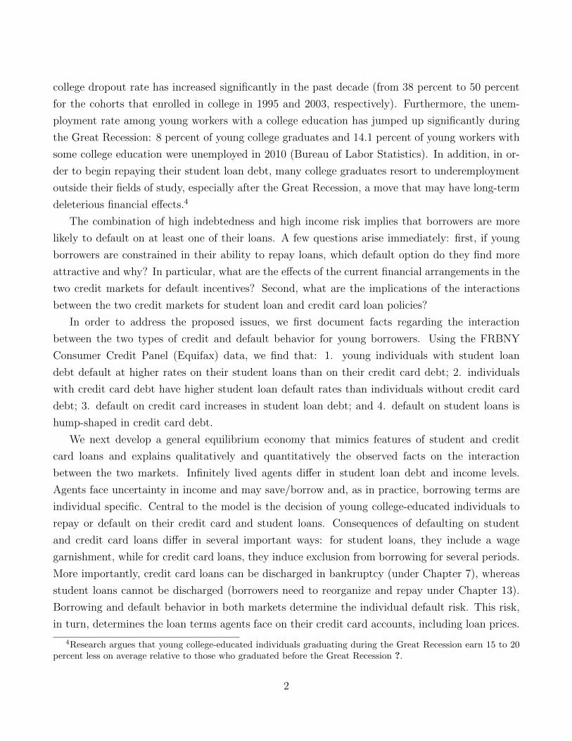
4. Default on credit card debt increases in student loan debt

As shown in Figure 2, credit card default increases with student loan debt from 1.75 percent

for individuals in the bottom decile of student loan debt to 2.4 percent for individuals in the

top decile of student loan debt.

The focus of our paper is on explaining the four facts documented above. However, there

are several additional facts that are relevant to our study and that we describe below. We note

that, unlike the four main facts described before, these additional facts have been documented in

previous studies.

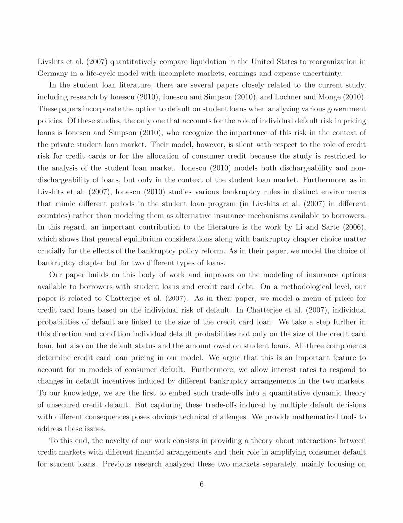
1. Default on credit card debt increases in credit card debt (fact A1).

According to our findings from Equifax credit card default increases from 0.1 percent to 4.2

percent (see Figure 3). This fact is in line with evidence in a series of papers (see Athreya

et al. (2009), Chatterjee et al. (2007), Han and Li (2011), Musto and Souleles (2006)).

2. Evidence on the relationship between default on student loans and student loan debt is mixed:

Dynarsky (1994) and Ionescu (2008) document that default on student loans is increasing in

10Note that we present these facts and figures based on an average over years 2004-2007 for non-homeowners aged20-45. Our findings, however, are robust to alternative years and age group specifications.

9

Figure 2: Credit card default by student loan debt

student loan debt. Our findings from Equifax show the opposite (fact A2).

3. Low income increases the likelihood of default on credit card debt (see Sullivan et al. (2001))

(fact A3).

4. Individuals with high credit risk receive higher interest rates on their credit card debt (Chat-

terjee et al. (2010)) (fact A4).

Figure 3: Credit card default by credit card debt

Lastly, there is a third set of facts on the trends in the two credit markets, facts that motivate

our study. To keep focus on the main facts of interest, however, we present this last set of facts in

the Appendix.

10

2.1 Institutional features

The main reported cause of bankruptcy is shocks to income and expenses. Sullivan, Warren, and

Westbrook (2000) report that 67.5 percent of filers claimed the main cause of their bankruptcy to

be job loss, while 22.1 percent cited family issues such as divorce and 19.3 percent blamed medical

expenses (multiple responses were permitted).

American households can choose between two bankruptcy procedures: Chapter 7, “liquidation”

bankruptcy and Chapter 13, ‘‘reorganization’’ bankruptcy. Approximately 70 percent of consumer

bankruptcies are filed under Chapter 7. Under Chapter 7, all unsecured debt is discharged in

exchange for noncollateralized assets above an exemption level. Debtors are not obliged, however,

to use future income to repay debts. Debtors must wait at least six years between Chapter 7

filings. While the majority of credit card default in the U.S. is under Chapter 7, only Chapter 13

bankruptcy applies to student loans. This action requires the reorganization and repayment of de-

faulted loans. Under the current Federal Student Loan Program (FSLP), students who participate

cannot discharge on their student loans except in extreme circumstances. Loan forgiveness is very

limited. It is granted only in the case that constant payments are made for 25 years or in the case

that repayment causes undue hardship. As a practical matter, it is very difficult to demonstrate

undue hardship unless the defaulter is physically unable to work. Partial dischargeability occurs

in less than 1 percent of the default cases.

In addition, eligibility conditions are very different for credit card and student loans and default

has different consequences in each market. Specifically, unlike credit card loans, government-

guaranteed student loans are conditioned on financial need, not credit ratings. Agents are eligible

to borrow up to the full college cost minus expected family contributions. Once borrowers are out

of college, they enter a standard 10-year repayment plan with fixed payments. The interest rate

on student loans does not incorporate the risk that some borrowers might exercise the option to

default. The interest rate is set by the government. Several default penalties implemented in the

student loan program might bear part of the default risk. In particular, consequences to defaulting

include wage garnishments (as high as 15 percent of the defaulter’s wages), seizure of federal tax

refunds, possible holds on transcripts and ineligibility for future student loans.

In contrast, credit card issuers use consumer repayment and borrowing behavior on all types

of loans to assess the likelihood that any single borrower will default (as reflected by FICO scores)

and price credit card loans accordingly.11

11For a comprehensive description of the two bankruptcy chapters for credit card loans see Li and Sarte (2006)and for student loans see Ionescu (2009). Also, in recent work, Eraslan, Kosar, Li, and Sarte (2014) present a niceanatomy of Chapter 13 Bankruptcy.

11

3 Model

3.1 Legal environment

Consumers who participate in the student loan and credit card markets, namely, young college

educated individuals with student loans, are small, risk-averse, price takers. They differ in levels

of student loan debt, d and income, y. They are endowed with a line of credit, which they may

use for transactions and consumption smoothing. They choose to repay or default on their student

loans as well as on their credit card debt.

3.1.1 Credit cards

Bankruptcy for credit cards in the model resembles Chapter 7 ‘‘total liquidation’’ bankruptcy. As

in practice, loan prices and credit limits imposed by credit card issuers are set to account for the

individual default risk and are tailored to each credit account. Consider a household that starts the

period with some credit card debt, bt. Depending on the household decision to declare bankruptcy

as well as on the household borrowing behavior, the following things happen:

1. If a household files for bankruptcy, λb = 1, then the household unsecured debt is discharged

and liabilities are set to 0.

2. The household cannot save during the period when default occurs, which is a simple way of

modeling that U.S. bankruptcy law does not permit those invoking bankruptcy to simulta-

neously accumulate assets.

3. The household begins the next period with a record of default on credit cards. Let ft ∈ F =

{0, 1} denote the default flag for a household in period t, where ft = 1 indicates in period t

a record of default and ft = 0 denotes the absence of such a record. Thus a household who

defaults on credit in period t starts period t+ 1 with ft+1 = 1.

4. A household who starts the period with a default flag cannot borrow and the default flag

can be erased with a probability pf .

5. In contrast, a household who starts the period with ft = 0 is allowed to borrow and save

according to individual credit terms: credit rates assigned to households by credit lenders

vary with individual characteristics. This feature is important to allow for capturing default

risk pricing in equilibrium.

12

This formulation captures the idea that there is restricted market participation for borrowers who

have defaulted in the credit card market relative to borrowers who have not. It also implies more

stringent credit terms for consumers who take on more credit card debt, i.e. precisely the type of

borrowers who are more constrained in their capability to repay their loans. In addition, creditors

take into account borrowing behavior in the other type of market, i.e. the student loan amount

owed, dt as well as the default status for student loans, ht. These features are consistent with the

fact that credit card issuers reward good repayment behavior and penalize bad repayment behavior,

taking into account this behavior in all markets in which borrowers participate. Finally, we assume

that defaulters on credit cards are not completely in autarky, which is consistent with evidence. In

U.S. consumer credit markets, households retain a storage technology after bankruptcy, namely,

the ability to save. We assume that without loss of generality, defaulters cannot borrow. In

practice, borrowers who have defaulted in the past several years are still able to obtain credit at

worse terms. In our model, allowing them a small negative amount or 0 does not have an effect

on the results.

3.1.2 Student loans

Bankruptcy for student loans in the model resembles Chapter 13 ‘‘reorganization’’ bankruptcy. As

in practice, default on student loans in the model at period t (denoted by λd = 1) simply means a

delay in repayment that triggers the following consequences:

1. There is no debt repayment in period t. However, the student loan debt is not discharged.

The defaulter must repay the amount owed for payment in period t+ 1.

2. The defaulter is not allowed to borrow or save in period t, which is in line with the fact that

credit bureaus are notified when default occurs and thus access to the credit card market

is restricted. Also, as in the case of the credit card market, this feature captures the fact

that U.S. bankruptcy law does not permit those invoking bankruptcy to simultaneously

accumulate assets.

3. A fraction γ of the defaulter’s wages is garnished starting in period t+ 1. Once the defaulter

rehabilitates her student loan, the wage garnishment is interrupted. This penalty captures

the default risk for student loans in the model.

4. The household begins the next period with a record of default on student loans. Let ht ∈H = {0, 1} denote the default flag for a household in period t, where ht = 1 indicates a

record of default and ht = 0 denotes the absence of such a record. Thus a household who

defaults in period t starts period t+ 1 with ht+1 = 1.

13

5. A household that begins period t with a record of default must pay the debt owed in period

t, dt. The default flag is erased with probability ph.12

6. There are no consequences on credit card market participation during the periods after a

default on student loan occurs. However, there are consequences on the pricing of credit card

loans from defaulting on student loans, as mentioned above. This assumption is justified by

the fact that in practice, student loan default is reported to credit bureaus and so creditors can

observe the default status immediately after default occurs. However, immediate repayment

and rehabilitation of the defaulted loan will result in the removal of the default status reported

by the loan holder to the national credit bureaus. In practice, the majority of defaulters

rehabilitate their loans. Therefore, they are still able to access the credit card market (on

worse terms, as explained above).

3.2 Preferences and endowments

At any point in time the economy is composed of a continuum of infinitely lived households with

unit mass.13 Agents differ in student loan payment levels, d ∈ D = {dmin, ..., dmax} and income

levels, y ∈ Y = [ymin, ymax]. There is a constant probability (1 − ρ) that households will die

at the end of each period. Households that do not survive are replaced by newborns who have

not defaulted on student loans (h = 0) or credit cards (f = 0), have zero assets (b = 0), and

with labor income and student loan debt drawn independently from the probability measure space

(Y × D,B(Y × D), ψ) where B(·) denotes the Borel sigma algebra and ψ = ψy × ψd denotes the

joint probability measure. Surviving households independently draw their labor income at time t

from a stochastic process. The amount that the household needs to pay on her student loan is the

same.14 Household characteristics are then defined on the measurable space (Y ×D,B(Y ×D)).

The transition function is given by Φ(yt+1)δdt(dt+1), where Φ(yt) is an i.i.d. process and δd is the

probability measure supported at d.

This assumption ensures that even for the worst possible realization of income, the amount

owed on student loans each period does not exceed the per period income.15

12The household cannot default the following period after default occurs. As mentioned before, less than 1 percentof borrowers repeat default, given that the U.S. government seizes tax refunds in the case that the defaulter doesnot rehabilitate her loan soon after default occurs. This penalty is severe enough to induce immediate repaymentafter default.

13The use of infinitely lived households is justified by the fact that we focus on the cohort default rate for youngborrowers, which means that age distributions are not crucial for analyzing default rates in the current study. Theuse of a continuum of households is natural, given the size of the credit market.

14Federal student loan payments are fixed and computed based on a fixed interest rate and duration of the loan.15This assumption is made for expositional purposes and is not crucial for the results. In fact, all results go

14

The preferences of the households are given by the expected value of a discounted lifetime

utility, which consists of:

E0

∞∑t=0

(ρβ)tU(ct) (1)

where ct represents the consumption of the agent during period t, β ∈ (0, 1) is the discount factor,

and ρ ∈ (0, 1) is the survival probability.

Assumption 1. The utility function U(·) is increasing, concave, and twice differentiable. It also

satisfies the Inada condition: limc→0+ U(c) = −∞ and limc→0+ U′(c) =∞.

3.3 Market arrangements

There are several similarities as well as important differences between the credit card market and

the market for student loans.

3.3.1 Credit cards

The market for privately issued unsecured credit in the United States is characterized by a large,

competitive marketplace in which price-taking lenders issue credit through the purchase of secu-

rities backed by repayments from those who borrow. These transactions are intermediated prin-

cipally by credit card issuers. Given a default option and consequences on the credit record from

default behavior, the market arrangement departs from the conventional modeling of borrowing

and lending. As in Chatterjee et al. (2007), our model handles the competitive pricing of default

risk, a risk that varies with household characteristics.16 In this dimension, our model departs from

Chatterjee et al. (2007) in several important ways: the default risk is based on the borrowing

behavior in both markets, i.e. it depends on the size of the loan on credit cards, bt as well as the

amount of student loans owed, dt. In addition, it depends on the default status on student loans,

ht. Competitive default pricing is achieved by allowing prices to vary with all three elements. This

modeling feature is novel in the literature and is meant to capture the fact that in practice, the

price of the loan depends on past repayment and borrowing behavior in all the markets in which

borrowers participate. Unsecured credit card lenders use this behavior (which, in practice, is cap-

tured in a credit score) as a signal for household credit risks and thus their probability of default.

through if this assumption is relaxed. Details are provided in the Appendix.16Chatterjee et al. (2007) handle the competitive pricing of default risk by expanding the “asset space” and

treating unsecured loans of different sizes for different types of households (of different characteristics) as distinctfinancial assets.

15

They tailor loan prices to individual default risk, not only to individual loan sizes. Obviously, in

the case of a default flag on credit cards, no loan is provided.

A household can borrow or save by purchasing a single one-period pure discount bond with a

face value in a finite set B ⊂ R. The set B = {bmin, . . . , bmax} contains 0 and positive and negative

elements. Let NB be the cardinality of this set. Individuals with ft = 1 (which is a result of

defaulting on credit cards in one of the previous periods) are limited in their market participation,

bt+1 ≥ 0.17

A purchase of a discount bond in period t with a non-negative face value bt+1 means that the

household has entered into a contract where it will receive bt+1 ≥ 0 units of the consumption

good in period t + 1. The purchase of a discount bond with a negative face value bt+1 means

that the household receives qdt,ht,bt+1(−bt+1) units of the period-t consumption good and promises

to deliver, conditional on not declaring bankruptcy, −bt+1 > 0 units of the consumption good in

period t+ 1; if it declares bankruptcy, the household delivers nothing. The total number of credit

indexes is NB ×ND ×NH . Let the entire set of NB ×ND ×NH prices in period t be denoted by

the vector qt ∈ RNB×ND×NH . We restrict qt to lie in a compact set Q ≡ [0, qmax]NB×ND×NH where

0 < qmax < 1.

3.3.2 Student loans

Student loans represent a different form of unsecured credit. First, loans are primarily provided

by the government (either direct or indirect and guaranteed through the FSLP), and do not share

the features of a competitive market.18 Unlike credit cards, the interest rate on student loans,

rg is set by the government and does not reflect the risk of default in the student loan market.19

However, the penalties for default capture some of this risk. In particular, the wage garnishment

is adjusted to cover default. More generally, loan terms are based on financial need, not on default

risk. Second, taking out student loans is a decision made during college years. Once households

are out of college, they need to repay their loans in equal rounds over a determined period of

17Note that households are liquidity constrained in the model. The existence of such constraints in credit cardmarkets has been documented by Gross and Souleles (2002). Overall credit availability has not decreased alongwith bankruptcy rates over the past several years before the Great Recession, so aggregate response of credit supplyto changing default has not been that large (see Athreya (2002)).

18Recently, students have started to use pure private student loans not guaranteed by the government. This newmarket is a hybrid between government loans and credit cards, featuring characteristics of both markets. However,this new market is still small and concerns about the national default rates are specific to student loans in thegovernment program, because default rates for pure private loansare of much lower magnitudes (for details seeIonescu and Simpson (2010)). Therefore, we focus on Federal student loans in the current study.

19Interest rates on Federal student loans are set in statute (after the Higher Education Reconciliation Act of 2005was passed). Details are provided in Section 5.

16

time subject to the fixed interest rate. We model college-loan-bound households that are out of

school and need to repay d per period; there is no borrowing decision for student loans.20 Third,

defaulters cannot discharge their debt. Recall that in the case that the household has a default

flag (h = 1), a wage garnishment is imposed and she keeps repaying the amount owed during the

following periods after default occurs.

We define the state space of credit characteristics of the households by S = B × F × H to

represent the asset position, the credit card, and student loan default flags. Let NS = NB × 2× 2

be the cardinality of this set.

To this end, an important note is that the assumption that all debt that young borrowers

access is unsecured is made for a specific purpose and is not restrictive. The model is designed to

represent the section of households who have student loans and credit card debt. As argued, these

borrowers rely on credit cards to smooth consumption and have little or no collateral debt.

3.4 Decision problems

The timing of events in any period is: (i) idiosyncratic shocks, yt are drawn for survivors and

newborns and student loan debt is drawn for newborns; (ii) households’ decisions take place:

they choose to default/repay on both credit card and student loans, make borrowing/savings and

consmkuption decisions, and default flags for the next period are determined. We focus on steady

state equilibria where qt = q.

3.4.1 Households

We present the households’ decision problem in a recursive formulation where any period t variable

xt is denoted by x and its period t+ 1 value by x′.

Each period, given their student loan debt, d, current income, y, and beginning-of-period

assets, b, households must choose consumption, c and asset holdings to carry forward into the next

period, b′. In addition, agents may decide to repay/default on their student loans, λd ∈ {0, 1} and

credit card loans, λb ∈ {0, 1}. As described before, these decisions have different consequences:

while default on student loans implies a wage garnishment γ and no effect on market participation

(although it may deteriorate terms on credit card accounts), default on credit card payments

triggers exclusion from borrowing for several periods and has no effect on income.

The household’s current budget correspondence, Bb,f,h(d, y; q) depends on the exogenously given

income, y, student loan debt, d, beginning of period asset position, b, credit card default record, f ,

20While returning to school and borrowing another round of loans is a possibility, this decision is beyond thescope of the paper.

17

student loan default record, h, and the prices in the credit card market, q. It consists of elements

of the form (c, b′, h′, f ′, λd, λb) ∈ (0,∞)×B ×H × F × {0, 1} × {0, 1} such that

c+ qd,h,b′ b′ ≤ y(1− g)− t+ b(1− λb)− d(1− λd),

and such that the following cases hold:

1. If a household with income y and student loan debt d has a good student loan record, h = 0,

and a good credit card record, f = 0, then we have the following: λd ∈ {0, 1} and λb ∈ {0, 1} if

b < 0 and λb = 0 if b ≥ 0. In the case where λd = 1 or λb = 1 then b′ = 0 and in the case where

λd = λb = 0 then b′ ∈ B. Also g = 0, h′ = λd, f′ = λd. The household can choose to pay off both

loans (λb = λd = 0), in which case the household can borrow freely on the credit card market. If

the household chooses to exercise its default option on either of the loans (λd = 1 or λb = 1), then

the household cannot borrow or accumulate assets. Since h = 0, there is no income garnishment

(g = 0).

2. If a household with income y and student loan debt d has a good student loan record, h = 0,

and a bad credit card record, f = 1, then λb = 0, λd ∈ {0, 1}, b′ ≥ 0, g = 0, h′ = λd, f′ = 1. In

this case, there is no repayment on credit card debt; the household chooses to pay or default on

the student loan debt. The household cannot borrow and the credit card record will stay 1.

3. If a household with income y and student loan debt d has a bad student loan record, h = 1,

and a good credit card record, f = 0, then λb ∈ {0, 1} if b < 0 and λb = 0 if b ≥ 0, λd = 0, g = γ,

f ′ = λb, and h′ = 1. The household pays back the credit card debt (if net liabilities, b < 0) or

defaults, pays the student loan and has its income garnished by a factor of γ. The student record

will stay 1. As in case 1, b′ ∈ B if λb = 0 and b′ = 0 if λb = 1.

4. If a household with income y and student loan debt d has a bad student loan record, h = 1,

and a bad credit card record, f = 1, then λd = λb = 0, b′ ≥ 0, g = γ, f ′ = 1, h′ = 1. The household

cannot borrow in the credit card market, pays the student loan, and has her income garnished.

There are several important observations: 1) we account for the fact that the budget constraint

may be empty; in particular ,if the household is deep in debt, earnings are low, and new loans

are expensive, then the household may not be able to afford non-negative consumption. The

implication of this is that involuntary default may occur; and 2) Repeated default on student loans

occurs on a limited basis (i.e. when Bb,f,1(d, y; q) = ∅) and is followed by partial dischargeability,

an assumption that is in line with the data. All households pay taxes t.

Assumption 2. We assume that consuming ymin today and starting with zero assets, b = 0 and a

bad credit card record, f = 1 and student loan default record, h = 1 with garnished wages (i.e. the

worst utility with a feasible action) gives a better utility than consuming zero today and starting

18

next period with maximum savings, bmax and a good credit card record, f = 0 and student loan

default record, h = 0 (i.e. the best utility with an unfeasible action).

Let v(d, y; q)(b, f, h) or vb,f,h(d, y; q) denote the expected lifetime utility of a household that

starts with student loan debt d and earnings y, has asset b, credit card default record f , and student

loan default record h, and faces prices q. Then v is in the set V of all continuous functions v :

D×Y ×Q→ RNS . The household’s optimization problem can be described in terms of an operator

(Tv)(d, y; q)(b, f, h) which yields the maximum lifetime utility achievable if the household’s future

lifetime utility is assessed according to a given function v(d, y; q)(b, f, h).

Definition 1. For v ∈ V , let (Tv)(d, y; q)(b, f, h) be defined as follows:

1. For h = 0 and f = 0

(Tv)(d, y; q)(b, f, h) = max(c,b′,h′,f ′,λd,λb)∈Bb,f,h(d,y;q)

U(c)− τbλb + βρ

ˆvb′,f ′,h′(d, y

′; q)Φ(dy′)

where τd and τb are utility costs that the household incurs in case of default in the student loan

market (τd) and in the credit card market (τb).

2. For h = 0 and f = 1 (in which case λb = 0 and f ′ = 1 with probability 1 − pf and f ′ = 0

with probability pf )

(Tv)(d, y; q)(b, f, h) = maxBb,f,h(d,y;q)

{U(c)− τdλd + (1− pf )βρ

ˆvb′,1,h′(d, y

′; q)Φ(dy′)

+ pfβρ

ˆvb′,0,h′(d, y

′; q)Φ(dy′)

}.

3. For h = 1 and f = 0 (in which case λd = 0 and h′ = 1 with probability 1 − ph and h′ = 0

with probability ph)

(Tv)(d, y; q)(b, f, h) = max

{max

Bb,f,h(d,y;q)

{U(c)− τbλb + (1− ph)βρ

ˆvb′,f ′,1(d, y

′; q)Φ(dy′)

+ phβρ

ˆvb′,f ′,0(d, y

′; q)Φ(dy′)

},

U(y)− τb + βρ

ˆv0,1,1(d, y

′; q)Φ(dy′)

}.

19

4. For h = 1 and f = 1

(Tv)(d, y; q)(b, f, h) = max

{max

Bb,f,h(d,y;q)

{U(c) + (1− pf )(1− ph)βρ

ˆvb′,1,1(d, y

′; q)Φ(dy′)

+(1− pf )phβρˆvb′,1,0(d, y

′; q)Φ(dy′)

+pf (1− ph)βρˆvb′,0,1(d, y

′; q)Φ(dy′)

pfphβρ

ˆvb′,0,0(d, y

′; q)Φ(dy′)

},

U(y) + βρ

ˆv0,1,1(d, y

′; q)Φ(dy′)

}.

The first part of this definition says that a household with good student loan and credit card

default records may choose to default on either type of loan, on both or on none of them. For all

these cases to be feasible, we need to have that the budget sets conditional on not defaulting on

student loans or on credit card debt are non-empty. In the case that at least one of these sets is

empty, then the attached option is automatically not available. In the case that both default and

no default options deliver the same utility, the household may choose either. Finally, recall that

in the case that the household chooses to repay her student loans or her credit card debt, she may

also choose borrowing and savings, and in the case that she decides to default on either of these

loans there is no choice on assets position.

The second part of the definition says that if the household has a good student loan default

record and a default flag on credit cards, she will only have the choice to default/repay on student

loans since she does not have any credit card debt. Recall that as long as the household carries

the default flag in the credit card market, she cannot borrow.

The last two parts represent cases for a household with a bad student loan default record. In

these last cases, defaulting on student loans is not an option. In part three, the household has the

choice to default on her credit card loan. As before, this is only an option if the associated budget

set is non-empty. In the case that all of these sets are empty, then default involuntarily occurs. We

assume that when involuntarily default happens it will occur on both markets (this is captured in

the second term of the maximization problem).21

In part four, however, there is no choice to default given that f = 1 and h = 1. Thus,

the household simply solves a consumption/savings decision if the budget set conditional on not

defaulting on either loan is non-empty. Otherwise, we assume that default involuntarily occurs. In

21This assumption is made such that default is not biased towards one of the two markets.

20

this case, this happens only in the student loan market since there is no credit card debt.

There are two additional observations: First, in all the cases in which default occurs on credit

card debt, the household incurs a utility cost, which is denoted by τb. Consistent with modeling

of consumer default in the literature, these utility costs are meant to capture the stigma following

default as well as the attorney and collection fees associated with default.22 Second, involuntary

default happens when borrowers with very low income realizations and high indebtedness have no

choice but default. Note that this case occurs repeatedly in the student loan market, i.e. for a

household with default flag, h = 1. Under these circumstances we assume that the household may

discharge her student loan and there is no wage garnishment. This feature captures the fact that

in practice, a small proportion of households partially discharge their student loan debt.

3.4.2 Financial intermediaries

The (representative) financial intermediary has access to an international credit market where it

can borrow or lend at the risk-free interest rate r ≥ 0. The intermediary operates in a competitive

market, takes prices as given, and chooses the number of loans ξdt,ht,bt+1 for all type (dt, ht, bt+1)

contracts for each t to maximize the present discounted value of current and future cash flows∑∞t=0(1 + r)−tπt, given that ξd−1,h−1,b0 = 0. The period t cash flow is given by

πt = ρ∑

dt−1,ht−1

∑bt∈B

(1− pbdt−1,ht−1,bt)ξdt−1,ht−1,bt(−bt)−

∑dt,ht

∑bt+1∈B

ξdt,ht,bt+1(−bt+1)qdt,ht,bt+1 (2)

where pbdt,ht,bt+1is the probability that a contract of type (dt, ht, bt+1) where bt+1 < 0 experiences

default; if bt+1 > 0, automatically pbdt,ht,bt+1= 0. These calculations take into account the survival

probability ρ.

If a solution to the financial intermediary’s problem exists, then optimization implies qdt,ht,bt+1 ≤ρ

(1+r)(1− pbdt,ht,bt+1

) if bt+1 < 0 and qdt,ht,bt+1 ≥ ρ(1+r)

if bt+1 ≥ 0. If any optimal ξdt,ht,bt+1 is nonzero

then the associate conditions hold with equality.

3.4.3 Government

The only purpose of the government in this model is to operate the student loan program. The

government needs to collect all student loans. The cost to the government is the total amount

of college loans plus the interest rate subsidized in college.23 Denote by L this loan price. We

22See Athreya et al. (2009), Chatterjee et al. (2007), and Livshits et al. (2007).23The government pays for the interest accumulated during college for subsidized loans but does not pay interest

for unsubsidized loans. For simplicity and ease of comparability, we assume that all student loans were subsidized.

21

compute the per period payment on student loans, d as the coupon payment of a student loan with

its face value equals to its price (a debt instrument priced at par) and infinite maturity (console).

Thus the coupon rate equals its yield rate, rg. In practice, this represents the government interest

rate on student loans. When no default occurs, the present value of coupon payments from all

borrowers (revenue) is equal to the price of all the loans made (cost), i.e. the government balances

its budget.

However, since default is a possibility, the government’s budget constraint may not hold. In

this case the government revenue from a household in state b with credit card default status f ,

income y and student loan debt d is given by (1− pdd)d where pdd is the probability that a contract

of type d experiences default for student loans. The government will choose taxes, t to recover the

losses incurred when default for student loans arises. The budget constraint is then given by

ˆdψd(dd) =

ˆ[(1− pdd)dψd(dd) +

ˆtdµ

Taxes are lump-sum and equally distributed in the economy. They are chosen such that the budget

constraint balances. We turn now to the definition of equilibrium and characterize the equilibrium

in the economy.

3.5 Steady-state equilibrium

In this section we define a steady state equilibrium, prove its existence, and characterize the

properties of the price schedule for individuals with different default risks.

Definition 2. A steady-state competitive equilibrium is a set of non-negative price vector q∗ =

(q∗d,h,b′

), non-negative credit card loan default frequency vector pb∗ = (pb∗

d,h,b′), a non-negative stu-

dent loan default frequency p∗d, taxes, t∗, a vector of non-trivial credit card loan measures, ξ∗ =

(ξd,h,b′∗), decision rules b′∗(y, d, f, b, h, q∗), λ∗b(y, d, f, b, h, q

∗), λ∗d(y, d, f, b, h, q∗), c∗(y, d, f, b, h, q∗),

and a probability measure µ∗ such that:

1. b′∗(y, d, f, b, h, q), λ∗b(y, d, f, b, h, q), λ

∗d(y, d, f, b, h, q), c

∗(y, d, f, b, h, q) solve the household’s

optimization problem;

2. t∗ solves the government’s budget constraint;

3. pd∗d =´λ∗d(y, d, f, b, h)dµ∗(dy, d, df, db, dh) (government consistency);

Lucas and Moore (2007) find that there is little difference between subsidized and unsubsidized Stafford loans.

22

4. ξ∗ solves the intermediary’s optimization problem;

5. pb∗d,h,b′

=´λ∗b(y

′, d, 0, b

′, h′∗)Φ(dy

′)H∗(h, dh′) for b

′< 0 and pb∗

d,h,b′= 0 for b

′ ≥ 0 (intermediary

consistency);

6. ξ∗d,h,b′

=´

1{b′∗ (y,d,f,b,h,q∗)=b′}µ∗(dy, d, df, db, h) (market clearing conditions (for each type (d, h, b

′));

7. µ∗ = µq∗where µq∗ = Γq∗µq∗ (µ∗ is an invariant probability measure).

The computation of equilibrium in incomplete markets models has been made standard by a series

of papers including (Aiyagari, 1994) and (Huggett, 1993) and have been extensively used in recent

papers with the one by (Chatterjee et al., 2007) being the most related to the current study.

However, our computation is more involved than previous work because of the dimensionality of

the state vector, the non-trivial market clearing conditions, which include a menu of loan prices,

the condition for the government balancing budget as well as the interaction between the two types

of credit.

Next, we proceed as following: we provide a first set of results which contains the existence

and uniqueness of the household’s problem and the existence of the invariant distribution. The

second set of results contains the characterization of both default decisions in terms of household

characteristics and market arrangements. The last set of results contains the existence of the

equilibrium and the characterization of prices. We prove the existence of cross-market effects and

characterize how financial arrangements in one market affect default behavior in the other market.

All proofs are provided in the Appendix.

4 Results

Existence and uniqueness of a recursive solution to the household’s problem

Theorem 1. There exists a unique v∗ ∈ V such that v∗ = Tv∗ and

1. v∗ is increasing in y and b.

2. Default decreases v∗.

3. The optimal policy correspondence implied by Tv∗ is compact-valued, upper-hemicontinuous.

4. Default is strictly preferable to zero consumption and optimal consumption is always positive.

23

Since Tv∗ is a compact-valued upper-hemicontinuous correspondence, Theorem 7.6 in ? (Mea-

surable Selection Theorem) implies that there are measurable policy functions, c∗(d, y, ; q)(b, f, h),

b∗(d, y; q)(b, f, h), λ∗b(d, y; q)(b, f, h) and λ∗d(d, y; q)(b, f, h). These measurable functions determine

a transition matrix for f and f′, namely F ∗y,d,b,h,q : F × F → [0, 1]:

F ∗y,d,b,h,q(f, f′= 1) =

1 if λ∗b = 1

1− pf if λ∗b = 0 and f = 1

0 otherwise

F ∗y,d,b,h,q(f, f′= 0) =

0 if λ∗b = 1

pf if λ∗b = 0 and f = 1

1 otherwise

The policy functions determine a transition matrix for the student loan default record, H∗y,d,b,f,q :

H ×H → [0, 1] which gives the student loan record for the next period, h′:

H∗y,d,b,f,q(h, h′

= 1) =

1 if λ∗d = 1 and h = 0

1− ph if h = 1

0 otherwise,

H∗y,d,b,f,q(h, h′

= 0) =

0 if λ∗d = 1 and h = 0

ph if h = 1

1 otherwise.

Existence of invariant distribution

Let X = Y × D × B × F × H be the space of household characteristics. In the following we

will write F ∗q (y, d, b, h, f, f ′) := F ∗y,d,b,h,q(f, f′) and H∗q (y, d, b, f, h, h′) := H∗y,d,b,f,q(h, h

′). Then the

transition function for the surviving households’ state variable TS∗q : X × B(X) → [0, 1] is given

by

TS∗q (y, d, b, f, h, Z) =

ˆZy×Zd×Zf×Zh

1{b∗∈Zb}F∗q (y, d, b, h, f, df

′)H∗q (y, d, b, f, h, dh

′)Φ(dy

′)δd(d

′)

24

where Z = Zy × Zd × Zb × Zf × Zh and 1 is the indicator function. The households that die

are replaced with newborns. The transition function for the newborn’s initial conditions, TN∗q :

X × B(X)→ [0, 1] is given by

TN∗q (y, d, b, f, h, Z) =

ˆZy×Zd

1{(b′ ,h′ ,f ′ )=(0,0,0)}Ψ(dy′, dd

′)

Combining the two transitions, we can define the transition function for the economy, T ∗q : X ×B(X)→ [0, 1] by

T ∗q(y, d, b, f, h, Z) = ρTSq(y, d, b, f, h, Z) + (1− ρ)TNq(y, d, b, f, h, Z)

Given the transition function T ∗q , we can describe the evolution of the distribution of households µ

across their state variables (y, d, b, f, h) for any given prices q. Specifically, let M(x) be the space

of probability measures on X. Define the operator Γq :M(x)→M(x):

(Γqµ)(Z) =

ˆT ∗q ((y, d, b, f, h), Z)dµ(y, d, b, f, h).

Theorem 2. For any q ∈ Q and any measurable selection from the optimal policy correspondence

there exists a unique µq ∈M(x) such that Γqµq = µq.

4.1 Characterization of the default decisions

We first determine the set for which default occurs for student loans (including involuntary default

with partial dischargeability), the set for which default occurs for credit card debt, as well as the set

for which default occurs for both of these two loans. Let DSLb,f,1(q) be the set for which involuntary

default on student loans and partial dischargeability occurs. This set is defined as combinations of

earnings, y, and student loan amount, d, for which Bb,f,1(d, y; q) = ∅ in the case h = 1. For h = 0

let DSLb,f,0(d; q) be the set of earnings for which the value of defaulting on student loans exceeds the

value of not defaulting on student loans. Similarly, let DCCb,0,h(d; q) be the set of earnings for which

the value of defaulting on credit card debt exceeds the value of not defaulting on credit card debt

in the case f = 0. Finally, let DBothb,0,0 (d; q) be the set of earnings for which default on both types of

loans occurs with h = 0 and f = 0. Note that the last two sets are defined only in the case f = 0,

since for f = 1 there is no credit card debt to default on.

Theorem 3 characterizes the sets when default on student loans occurs (voluntarily or involun-

tarily). Theorem 4 characterizes the sets when default occurs on credit card debt and Theorem 5

25

presents the set for which default occurs for both types of loans.

Theorem 3. Let q ∈ Q, b ∈ B. If h = 1 and the set DSLb,f,1(q) is nonempty, then DSL

b,f,1(q) is closed

and convex. In particular, the sets DSLb,f,1(d; q) are closed intervals for all d. If h = 0 and the set

DSLb,f,0(d; q) is nonempty, then DSL

b,f,0(d; q) is a closed interval for all d.

Theorem 4. Let q ∈ Q, (b, 0, h) ∈ S. If DCCb,0,h(d; q) is nonempty then it is a closed interval for all

d.

Theorem 5. Let q ∈ Q, (b, 0, 0) ∈ S. If the set DBothb,0,0 (d; q) is nonempty then it is a closed

interval for all d.

Next, we determine how the set of default on credit card debt varies with the credit card debt,

the student loan debt, and the default status on student loans of the individual. Specifically,

Theorem 6 shows that the set of default on credit card debt expands with the amount of debt for

credit cards. This result was first demonstrated in Chatterjee et al. (2007).

Theorem 6. For any price q ∈ Q, d ∈ D, f ∈ F , and h ∈ H, the sets DCCb,f,h(d; q) expand when b

decreases.

In addition, we show two new results in the literature: 1) the set of default on credit card loans

only shrinks when the student loan amount increases and the set of default on both credit card

and student loans expands when the student loan amount increases. These findings imply that

individuals with lower levels of student loans are more likely to default only on credit card debt

and individuals with higher levels of student loans are more likely to default on both credit card

and student loan debt (Theorem 7); and 2) the set of default on credit card loans is larger when

h = 1 relative to the case in which h = 0. This result implies that individuals with a default record

on student loans are more likely to default on their credit card debt (Theorem 8).

Theorem 7. For any price q ∈ Q, b ∈ B, f ∈ F , and h ∈ H, the sets DCCb,f,h(d; q) shrink and

DBothb,f,h (d; q) expand when d increases.

Theorem 8. For any price q ∈ Q, b ∈ B, d ∈ D, and f ∈ F , the set DCCb,f,0(d; q) ⊂ DCC

b,f,1(d; q).

This last set of theorems shows the importance of accounting for borrowing and default behavior

in the student loan market when determining the risk of default on credit card debt. These elements

will be considered in the decision of the financial intermediary, which we explain next.

26

4.2 Existence of equilibrium and characterization

Theorem 9. Existence A steady-state competitive equilibrium exists.

In equilibrium, the credit card loan price vector has the property that all possible face-value

loans (household deposits) bear the risk-free rate and negative face-value loans (household bor-

rowings) bear a rate that reflects the risk-free rate and a premium that accounts for the default

probability. This probability depends on the characteristics of the student loan markets, such as

loan amount and default status, as well as the size of the credit card loan. This result is delivered by

the free entry condition of the financial intermediary which implies that cross-subsidization across

loans made to individuals of different characteristics in the student loan market is not possible.

Each (d, h) market clears in equilibrium and it is not possible for an intermediary to charge more

than the cost of funds for individuals with very low risk in order to offset losses on loans made to

high risk individuals. Positive profits in some contracts would offset the losses in others, and so

intermediaries could enter the market for those profitable loans. We turn now to characterizing

the equilibrium price schedule.

Theorem 10. Characterization of equilibrium prices In any steady-state equilibrium, the

following is true:

1. For any b′ ≥ 0, q∗d,h,b′ = ρ/(1 + r) for all d ∈ D and h ∈ H.

2. If the grids of D and B are sufficiently fine, and h = 0, there are d > 0 and b′ < 0 such that

q∗d,h,b′ = ρ/(1 + r) for all d < d and b′> b′.

3. If the set of income levels for which the household is indifferent between defaulting on credit

card debt and any other available option is of measure zero, then d1 < d2 implies q∗d1,h,b′ >

q∗d2,h,b′ for any h ∈ H and b′ ∈ B.

4. If the set of income levels for which the household is indifferent between defaulting on credit

card debt and any other available option is of measure zero, then q∗d,h=1,b′ < q∗d,h=0,b′ for any

d ∈ D and b′ ∈ B.

Theorem 10 demonstrates that firms charge the risk-free interest rate on deposits (property

1) and on small loan sizes made to individuals with no default record on student loans and small

enough levels of student loans (property 2). Property 3 shows that individuals with lower levels

of student loans are assigned higher loan prices. The last property shows that individuals with a

default record on student loans pay higher prices than individuals with no default record for any

loan size, b′ and for any amount of student loans they owe, d.

27

4.3 The interplay between the two markets

Since the novel feature in this paper is the interaction between different types of unsecured credit

markets and its effects on default decisions, we show how the default decision varies not only with

the loan amount in the respective market, but also with the loan amount in the other market. We

already established that the default probability on credit card loans increases in the amount of

student loans. In this section we demonstrate that a borrower with high enough loans will prefer

defaulting on her student loans rather than on her credit card debt. Theorem 11 shows that we can

find a combination of credit card debt and student loan debt which induces a borrower to default.

Furthermore, if the amounts owed to student loans and credit card accounts are higher than the

two values in this combination, then the borrower will choose to default on student loans rather

than on credit card debt.

Theorem 11. If the grid of D is fine enough, then we can find d1 ∈ D and b1 ∈ B such that the

agent defaults. Moreover, we can find d2 ≥ d1 and b2 ≤ b1 such that the agent defaults on student

loans.

The intuition behind this result is that with high enough debt levels, consumption is very small

in the case that the agent does not default at all. Consequently, she finds it optimal to default. In

the case that the student loan amount and credit card debt are large, defaulting on student loans

is optimal since the option of defaulting on credit card debt triggers limited market participation.

Defaulting on credit card debt is too costly compared with the benefit of discharging one’s debt.

When borrowers find themselves in financial hardship and have to default, they choose to default

on student loans. They delay their repayments on student loans at the expense of having their

wage garnished in the future. But this penalty is less severe compared to being excluded from

borrowing for several periods. These are precisely the types of borrowers who most need the credit

card market to help them smooth out consumption.

To conclude, our theory produces several facts consistent with reality (presented in Section 2):

First, the incentive to default on student loans increases in student loan debt burden (debt-to-

income ratio), i.e. default on student loans is more likely to occur for individuals with low levels

of earnings and high levels of student loan debt. Second, the incentive to default on credit card

debt increases in credit card debt, which is consistent with findings in (Chatterjee et al., 2007).

Our theory is innovative because it shows that a household with a high amount of student loans

or with a record of default on student loans is more likely to default on credit card debt. This result

emphasizes the importance of accounting for other markets in which the individual participates

when studying default on credit card debt. Finally, we show that while a high student loan debt

28

burden is necessary to induce default on student loans, this effect is amplified by high indebtedness

in the credit card market. The financial arrangements in the two markets, and in particular the

differences in bankruptcy rules and default consequences between the two types of credit, certainly

play an important role in shifting default incentives. In the next section we quantify the role each

of these two types of credit played in the increase in student loan default rates in recent years.

5 Quantitative analysis

5.1 Mapping the model to the data

There are four sets of parameters that we calibrate: 1) standard parameters, such as the discount

factor and the coefficient of risk aversion; 2) parameters for the initial distribution of student loan

debt and income; 3) parameters specific to student loan markets such as default consequences and

interest rates on student loans; and 4) parameters specific to credit card markets. Our approach

includes a combination of setting some parameters to values that are standard in the literature,

calibrating some parameters directly to data, and jointly estimating the parameters that we do

not observe in the data by matching moments for several observable implications of the model.

Our model is representative for college-educated individuals who are out of college and have

student loans. We calibrate the model to 2004-2007 and use the Survey of Consumer Finances in

2004 and 2007 for moments in the distribution of income, student loan, and credit card debt. The

sample consists of young households (aged 20-30 years old) with college education and student loan

debt. The age group is specifically chosen to include college dropouts and recent graduates. All

individuals are out of college and in the labor force. The sample sizes are 466 and 430, respectively.

All numbers in the paper are provided in 2004 dollars.24

The model period is one year and the coefficient of risk aversion chosen (σ = 2) is in the

range of estimates suggested by ? and ?. The discount factor (β = 0.96) is also standard in the

literature. We set the interest rate on student loans rg = 0.068 as the most representative rate for

student loans.25 The annual risk-free rate is set equal to rf = 0.04, which is the average return on

capital reported by McGrattan and Prescott (2000). Table 1 presents the basic parameters of the

model. We set the transaction cost in the credit card market to 0.053 following ?. We estimate

24We use both SCF 2004 and SCF 2007 for the benchmark calibration rather than only one of the two surveysto better capture the borrowing and default behavior before the Great Recession.

25The interest rate for Federal student loans was set to 6.8 percent in 2006 and it remained to this level forunsubsidized loans. The rate further decreased for new undergraduate subsidized loans after July 1, 2008. Before2006 the rate was variable, ranging from 2.4 to 8.25 percent. For details see ?.

29

Table 1: Parameter Values

Parameter Name Value Target/Source

σ Coef of risk aversion 2.00 standard

β Discount factor 0.96 standard

rg Interest on student loans 0.068 Dept. of Education

rf Risk-free rate 0.04 Avg rate 2004-2007 (FRB-G19)

φ Transaction cost 0.053 Evans and Schmalensee (1999)

pf Prob to keep CC default flag 0.9 Avg years of punishment=10

ph Prob to keep SL default flag 0.5 Avg years of punishment=2

ρ Survival probability 0.975 Avg years of life=40

γ Wage garnishment if SL default 0.028 Default rate on SL =5%

τp Utility loss from CC default 19.5 CC debt/income ratio=0.057

the survival probability ρ = 0.975 to match average years of life to 40.26 The probabilities to keep

default flags in the two markets are set to 1 − pf = 0.9 for credit card debt and 1 − ph = 0.5 for

student loan debt to match average years of punishments, ten for the credit card market and two

for the student loan market. The first is consistent with estimates in the literature (see Chatterjee

et al. (2007) and Livshits et al. (2007)) and the second is consistent with regulations from the

DoE. Specifically, it takes one period before borrowers restructure and reorganize and another

period before completing loan rehabilitation. Borrowers must make 10 consecutive payments to

rehabilitate. We assume that the default flag is immediately removed after rehabilitation. We

estimate the wage garnishment (γ) and the utility loss from defaulting on credit card loans (τp) to

match the two year cohort default rate for student loans of 5 percent during 2004-2006 (see Figure

2 in section 2.2) and the credit card debt to income ratio in our sample from SCF.27

We use the joint distribution of student loan debt and income for young households as delivered

by the SCF 2004 and SCF 2007. The mean of income is $51,510 and the standard deviation

$41,688. The mean amount of student loan debt owed per period is $2,741 and the standard

deviation $2,400. We assume a log normal distribution with parameters (µy, σy, µd, σd, ρyd) =

(0.3212, 0.2633, 0.0174, 0.0153, 0.2633) on [0, 1]× [0, 0.12].28 We pick the grid for assets consistent

with the distribution of credit card debt in the SCF 2004-2007, for which the mean and standard

deviations are $2,979 and $4,934, respectively.

26Since our agents are 27 years old, this calibration matches a lifetime expectancy of 67 years old.27Our estimate is in line with the data where the garnishment can be anywhere from 0 to 15 percent. Also, as in

practice, wage garnishments do not apply if income levels are below a minimum threshold below which the borrowerexperiences financial hardship.

28We normalize $163,598=1. This represents the maximum level of income which is equal to mean of income plus3 times the standard deviation of income.

30

5.2 Results: Benchmark economy

5.2.1 Model versus data

The model does a good job of matching debt burdens in the two markets for borrowers in the SCF

2004-2007. It delivers a credit card debt burden of 0.056 and a student loan debt burden of 0.054.

The data counterparts are 0.058 and 0.054, respectively. The model predicts that 18 percent of

individuals have negative assets (without including student loans). The data counterpart is 34

percent.29

Table 2: Data versus model

Data Model

Credit card default rate 0.6% 0.33%

Credit card interest rate 12% 9.8%

Per period college debt-to-income ratio (exog) 0.054 0.054

Credit card debt-to-income ratio (targeted) 0.057 0.056

Student loan default rate (targeted) 5% 5%

Also, the model replicates the distribution of credit card debt and credit card interest rate quite

well , as evident in Figure 4. The model delivers an average credit card debt of $2,990 and an

average credit card interest rate of 9.8 percent. The data counterparts are $2,979 and 12 percent,

respectively. The interest rate in the model is lower compared to the credit card rate in the data

since the interest rate in the model represents the effective rate at which borrowers pay, whereas

in the data borrowers pay the high rate only in the case that they roll over their debt. The default

rate on credit card debt is 0.3 percent, which is in the range used in the literature (see Athreya

et al. (2009)). Lastly, taxes to cover defaulters in the economy are insignificant (3.615e-004 percent

of income, on average).

29This measure is computed using total unsecured debt (but excluding student loans) minus financial assets,defined as the sum of checking and savings accounts, money market deposit accounts, money market mutual funds,value of certificates of deposit, and the value of savings and bonds.

31

Figure 4: Distributions of credit card debt and interest rateModel versus data

0 2000 4000 6000 8000 10000 120000

1

2

3

4

5

6

7

8x 10

−4 CC Balance Distribution: Model versus Data

Model

SCF Data

0 0.05 0.1 0.15 0.2 0.25 0.3 0.35 0.40

2

4

6

8

10

12

14

CC Rate Distribution: Model versus Data

Model

SCF Data

5.2.2 Predictions for the interaction between the two types of debt and default

We next describe the model’s predictions regarding the interaction between the two types of debt

and default. The model successfully predicts all four main facts of interest to our study, which are

described in Section 2.

1. First, the model predicts that default on student loans is higher than default on credit card

debt (5 percent versus 0.33 percent). Recall that the student loan default is targeted in the

calibration procedure, while the default on credit card debt is not. This prediction is a direct

implication of our main theoretical result that students prefer default on student loan debt to

default on credit card debt given less severe long term consequences to defaulting on student

loans.

2. Individuals with credit card debt have higher default rates for student loans (5.8 percent)

relative to individuals with no credit card debt (4.8 percent). Note that the gap in default

rates between the two groups is smaller in the model than in the data (recall that the data

counterparts are 5.75 percent versus 2.4 percent, respectively).

3. Conditional on having credit card debt, the model delivers a hump-shaped profile for student

loan default in credit card debt as Figure 5 shows.

Default rates vary quite significantly across individuals with different levels of credit card

debt, ranging from about 2 percent default rate for individuals in the top decile of credit

32

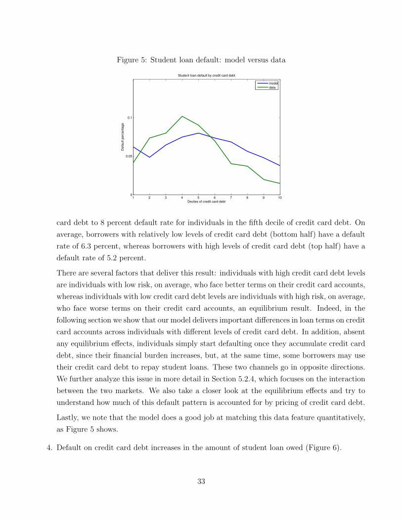
Figure 5: Student loan default: model versus data

1 2 3 4 5 6 7 8 9 100

0.05

0.1

Student loan default by credit card debt

Deciles of credit card debt

De

fault p

erc

en

tage

model

data

card debt to 8 percent default rate for individuals in the fifth decile of credit card debt. On

average, borrowers with relatively low levels of credit card debt (bottom half) have a default

rate of 6.3 percent, whereas borrowers with high levels of credit card debt (top half) have a

default rate of 5.2 percent.

There are several factors that deliver this result: individuals with high credit card debt levels

are individuals with low risk, on average, who face better terms on their credit card accounts,

whereas individuals with low credit card debt levels are individuals with high risk, on average,

who face worse terms on their credit card accounts, an equilibrium result. Indeed, in the

following section we show that our model delivers important differences in loan terms on credit

card accounts across individuals with different levels of credit card debt. In addition, absent

any equilibrium effects, individuals simply start defaulting once they accumulate credit card

debt, since their financial burden increases, but, at the same time, some borrowers may use

their credit card debt to repay student loans. These two channels go in opposite directions.

We further analyze this issue in more detail in Section 5.2.4, which focuses on the interaction

between the two markets. We also take a closer look at the equilibrium effects and try to

understand how much of this default pattern is accounted for by pricing of credit card debt.

Lastly, we note that the model does a good job at matching this data feature quantitatively,

as Figure 5 shows.

4. Default on credit card debt increases in the amount of student loan owed (Figure 6).

33

Figure 6: Credit card default: model versus data

1 2 3 4 5 6 7 8 9 100

0.002

0.004

0.006

0.008

0.01

0.012Credit card default by student loan debt

Deciles of student loan debt

De

fault p

erc

en

tage

The pattern matches the data and reveals that individuals with larger amounts of student loan

debt represent a higher risk for the credit card market. This result is delivered by the fact that

student loan debt simply represents an extra financial burden, which increases the likelihood of

default. In other words, two individuals with high and low levels of student loan debt, who have

the same amount of credit card debt and who are subjected to the same bad income shock will

have a higher (and lower, respectively) incentive to default. The same negative shock has a higher

(respectively, lower) effect on utility depending on the amount of debt owed in the student loan

market. While this prediction is consistent with the data fact 4 qualitatively, the default rates on

credit card debt in the model are smaller than those in the data. This is a consequence of the

measurement used in the data for default on credit card debt.30

5.2.3 Additional predictions for default behavior

The model’s predictions regarding default in each market and pricing are also consistent with

the facts presented in Section 2 (additional facts A1-A4). In particular, as shown in Figure 7,

default on credit card debt increases in credit card debt (fact A1) and default on student loans

increases with the amount of student loan debt. Recall that the evidence on the latter fact, A2, is

30Recall that absent a default measure per se in the data, we construct this measure for credit card default to beconsistent with the measure constructed for student loan debt (defined to match the default rate on student loansin the data). In reality (and thus in the model), default on credit card debt is more strictly defined.

34

mixed. Our model predicts that, the likelihood of default on student loans is significantly higher

for individuals with high levels of student loan debt relative to the default rate for individuals with

low student loan debt (9.08 percent versus 0.68 percent).

Lastly, the likelihood of default on credit card debt decreases with income, as Figure 7 shows,

result consistent with the empirical literature (fact A3). However, for the most part, theories of

unsecured default deliver the opposite result. The intuition behind this previous result in the

literature is that agents with relatively low income levels stand to lose more from defaulting on

their credit card debt relative to individuals with high income levels, for whom the penalties

associated with default are less costly in relative terms. In our model, however, individuals also

possess other types of loans, i.e. student loans with different default consequences; individuals in

our model make a joint default decision. It turns out that this interaction is key in delivering the

default probability in the credit market to decrease in income. This finding shows the importance

of accounting for other types of loans when analyzing default behavior, a feature that is absent in

previous models of consumer default. Details of the interaction between the two markets together

with the importance of income for default are discussed in more detail in Section 5.2.4.

5.2.4 Credit card pricing

To sum-up, our model predicts that default rates on credit card debt increase with both types of

loans. As evidenced in Figures 6 and 7, default on credit card debt is more sensitive to the debt

in the credit card market, but student loan amounts have important effects on the incentive to

default on credit card debt as well. In general, borrowers need high levels of debt in both markets

to induce default on credit card debt, given that this event occurs at a low frequency in our model.

In addition, we find that defaulters on student loans have a higher likelihood of default on credit

card debt relative to non-defaulters in the student loan market. There are two main reasons behind

this result: first, defaulters on student loans do not have the option to default on their student

loans, so if they must default they do so in the credit card market; and second, in addition to

being asked to repay their student loans, individuals with a default record on student loans also

have part of their earnings garnished.

Consistent with our results on the individual probability of default for credit cards, the model

delivers a pricing scheme of credit card loans based on individual default risk as proxied by the size

of the loan, the amount owed in the student loan market, and the default status in the student loan

market. Recall that our theoretical results show that the interest rate on credit card debt increases

in both amounts of loans and is higher for individuals with a default flag on student loans. These

results are consistent with fact A4 in Section 2 that borrowers with high risk are priced higher

35

Figure 7: Default behavior

1 2 3 4 5 6 7 8 9 100

0.002

0.004

0.006

0.008

0.01

0.012

0.014

0.016Credit card default by credit card debt

Deciles of credit card debt

Defa

ult p

erc

enta

ge

1 2 3 4 5 6 7 8 9 100

0.02

0.04

0.06

0.08

0.1

0.12

0.14

0.16

0.18

0.2Student loan default by student loan debt

Deciles of student loan debt

Defa

ult p

erc

enta

ge

1 2 3 4 5 6 7 8 9 100

0.005

0.01

0.015

1 2 3 4 5 6 7 8 9 100

0.005

0.01

0.015Credit card default by income

Income deciles

De

fault p

erc

enta

ge

36

rates than borrowers with low risk. This is indeed what our model delivers. Table 3 summarizes

our quantitative results regarding credit card loan pricing across these individual characteristics

for individuals with high levels of debt in each market (defined as the top 50th percentile) versus

individuals with low levels of debt (defined as the bottom 50th percentile).

Table 3: Credit card interest rates across individual characteristics

Characteristic Low High

CC debt 9.35% 10.1%SL debt 9.44% 10.3%

SL def flag(0/1) 9.7% 10%Income 9.8% 9.3%

First, agents with high levels of credit card debt (top 50th percentile) have a credit card rate

of 10.1 percent and agents with low credit card debt (bottom 50th percentile) have a credit card

rate of 9.35 percent. Second, agents with high levels of student loans receive a credit card rate of

10.3 percent and agents with low levels of student loans receive a credit card rate of 9.44 percent.

The wedge in the interest rates accounts for the gap in the probabilities of default between these

two groups (presented in Table 3). Finally, defaulters on student loans (h = 1) have a credit card

rate of 10 percent (in column “high” in Table 3) and nondefaulters on student loans (h = 0) have

a credit card rate of 9.7 percent (in column “low” in Table 3). We conclude that the amount of

student loan debt and the default status on student loans represent important components of credit

card loan pricing. These three findings represent the quantitative counterpart of our theoretical

results in Theorem 10. In addition, our quantitative analysis predicts that agents with low income

receive higher rates, on average, than agents with high income, as Table 3 shows. This is a direct

implication of the differences in default rates across income groups.

5.3 The interplay between the two markets

We turn now to the interaction between the two markets and its effect on default behavior. Recall

from Theorem 11 that in any steady-state equilibrium, we can find a combination of student loans

and credit card debt such that individuals default. Furthermore, if loan amounts in both markets

are larger than these two levels of debt, then default occurs on student loans. Our quantitative

analysis in this subsection complements this theoretical result.

First, recall that in our model, everyone who defaults on credit card debt also defaults on

student loan debt. There is no borrower who strictly prefers defaulting on credit card debt to

defaulting on student loans. Table 4 shows our findings regarding default behavior across groups

37

Table 4: Default rates across debt levels in the two markets

b ≥ 0 “b < 0 Low” “b < 0 High”

d “Low”Default SL 0.65% 0.85% 0.76%Default CC - 0 0.23%d “High”

Default SL 8.37% 14.8% 12.7%Default CC - 0.12% 1.1%

of student loan and credit card debt. We divide individuals in two groups based on the amount

owed to the student loan program, d (low and high defined as before) and in three groups based

on the credit card debt, b: one group with positive assets and two groups with negative assets (low

and high defined as before).

We find that individuals with no credit card debt have lower default rates on student loans

than individuals with credit card debt, regardless of the amount owed in the student loan market.

Second, conditional on having low levels of student loan debt, individuals with low levels of credit

card debt do not default on their credit card debt, but rather default on their student loans (if

they must default). The benefit of discharging their credit card debt upon default is too small

compared to the large cost of being excluded from borrowing. At the same time, the penalties

associated with default in the student loan market are not contingent on their credit card debt.

Similarly, conditional on having high levels of student loan debt, individuals with high levels of

credit card debt have a higher likelihood of defaulting on their credit card debt. Third, the gap

between default rates by student loan amounts is higher for individuals with low levels of credit

card debt relative to individuals with high levels of credit card debt.

These findings confirm our conjecture that while both types of debt increase incentives to

default in both credit markets, some individuals may substitute credit card debt for student loan

debt, in particular individuals with high levels of student loans. But these individuals with high

levels of student loans represent high risk for the credit card market and therefore receive worse

terms on their credit card accounts. More expensive credit card debt together with the need to

access the credit card market may increase incentives to default on student loans. We further

examine which individuals can use the credit card market to pay off student loan debt and which

ones are defaulting even more on their student loans because of more (and expensive) credit. We

determine combinations of student loans and credit card debt levels such that above these levels

of debt in the two markets, the incentives to default on student loans increase rapidly and no one

strictly prefers to default on their credit card debt. This is the quantitative counterpart of our

38

Figure 8: Default conditional on both types of debt

0

2

4

6

8

10

0

2

4

6

8

10

0

0.05

0.1

0.15

0.2

0.25

0.3

0.35

0.4

0.45

Credit card debt deciles

Student loan default by debt percentiles

Student loan debt deciles

Defa

ult p

erc

en

tag

e

0

2

4

6

8

10

0

2

4

6

8

10

0

0.05

0.1

0.15

0.2

0.25

0.3

0.35

0.4

Credit card debt deciles

Credit card default by debt percentiles

Student loan debt deciles

Defa

ult p

erc

en

tag

e

main theoretical result (Theorem 11), which showed that there exists a combination of student

loans (d1 ∈ D) and credit card debt (b1 ∈ B) such that above this threshold d1 individuals may

default first on their student loans. We determine such (d1, b1) combinations next. In addition,

our quantitative analysis establishes that under these thresholds d1 and b1, students may be able

to use the credit card market to pay off their student loan debt. These findings are evidenced in

Figure 8, which illustrates the default rates in the two markets conditional on both types of debt.

Note in the left panel of Figure 8 that for a borrower in the 10th decile of student loans, there

is a sharp increase in student loan default once the borrower has more credit card debt than in

the 5th decile. Similarly, for a borrower in the 9th (8th) decile of student loans, there is a rapid

increase in student loan default once the borrower has more debt than in the 6th (8th) decile of

credit card debt. Below these levels of credit card debt, however, default on student loans is quite

flat across deciles of credit card debt. These findings imply that before hitting a critical credit card

debt level, individuals are able to use the credit card market to keep their student loan default rate

low. Once they borrow more than this threshold level, their default on student loans is amplified

by their credit card debt. This threshold of credit card debt (or critical point) is decreasing with

student loan debt, in part because the interest rates on credit card loans increase with student

loan levels.

An interesting result is that for borrowers with intermediate levels of student loan debt (5th

and 6th deciles) default on student loans is hump-shaped in credit card debt levels. This result

suggests that these borrowers may use credit card debt to pay off their student loans. Their student

loan levels are high enough for them to need to borrow in the credit card market, but not high

39

enough to induce high default incentives; at the same time, terms on credit card accounts for these

individuals are good enough for them to be able to use the credit card market to keep student loan

default rates low. For individuals with very low levels of student loan debt, however, default on

student loans is flat across deciles of credit card debt. Their incentive to default on student loans

is very low and credit card debt does not affect this decision. The combination of these factors

delivers the hump-shaped student loan default pattern across levels of credit card debt (Figure 5).

This pattern is a result of a composition effect in addition to a strategic default effect. Borrowers

with high levels of credit card debt are mostly low risk individuals with low levels of student loans.

They receive lower interest rates and have higher levels of credit card debt in equilibrium. Finally,

credit card default increases with both levels of debt (right panel in Figure 8). As expected, a lower

credit card level is needed to trigger default on credit card debt for individuals with high levels of

student loans relative to individuals with low levels of student loans. Consistent with our theory,

all defaulters on credit card debt also default on their student loans.

We conclude that, on average, having debt in one of the two markets amplifies the incentives

to default in the other market. However, while student loan debt increases credit card default

regardless of loan amount, debt in the credit card market amplifies the incentive to default on

student loans only for certain combinations of debt. More importantly, some individuals may use

the credit card market to reduce their default on student loans. On the one hand, participating

in the credit card market and at worse terms pushes borrowers towards more default on their

student loans. On the other hand, taking on credit card debt helps student loan borrowers smooth

consumption and pay their student loan debt.

5.3.1 Importance of income

Certainly these channels work differently for individuals with different levels of income. We further

investigate this issue and present our findings in Figure 9. First, we find that individuals with

medium levels of income (top panel) have higher default rates on student loans than individuals

with low or high levels of income; in addition, having credit card debt further increases default

on student loans for most borrowers in this income group. Second, individuals with high income

levels (middle panel) have lower default rates on student loan debt. As expected, they need larger

amounts for both types of loans to default and their incentives to default on student loans are

amplified by having more credit card debt. Third, an interesting result is that for individuals with

low levels of income (bottom panel), incentives to default on student loans are not amplified by

credit card debt. On the contrary, poor individuals with large levels of student loans seem to

primarily use credit card debt to lower default on student loans. Notice the decline in default rates

40

for student loans across deciles of credit card debt for top deciles of student loans, shown in the

bottom panel.

Overall, individuals with medium levels of income default the most on their student loans (Fig-

ure 9). Those with high levels of income are not financially constrained and the wage garnishment

punishment is too costly for them to warrant default on their student loans, while individuals with

low levels of income would rather use the credit card market to pay off their student loans. Some

of these low income individuals may also default on their credit card debt. We conjecture that

various terms and changes in the credit market affect the default behavior in the student loan

market differently across income groups, especially during the Great Recession, when credit card

terms worsened and income was negatively affected. We analyze these issues in the next section.

5.3.2 Importance of credit card terms

We run two counterfactual experiments to asses the importance of terms (credit limits and interest

rates) on credit card accounts for default incentives on student loans.

To be completed.

5.4 Policy implications: Income contingent repayment

There are currently four versions of student loan repayment plans based on income.31 All of

these plans assume loan payments as a percentage of discretionary income. Borrowers who earn

less than 150 percent of the poverty line have a loan payment of zero (or $5 depending on the

income plan type).32 Borrowers who have an income higher than this threshold pay a fraction of

their income (between 10-25 percent depending on the income plan type). The income contingent

repayment plan (ICR) provides more flexibility in eligibility criteria and therefore is used in the

current experiment. According to the ICR borrowers pay 20 percent of discretionary income and

any remaining debt after 25 years in repayment is forgiven, including both principal and interest.

When the ICR was introduced in 2010 (The Health Care and Education Reconciliation Act of

2010) it resulted in a lot of discussions among policy makers, in particular regarding its cost.

We analyze the quantitative implications of the ICR in both normal times and in the Great

Recession. Our analysis takes into account the fact that the amount of student loans discharged

is recovered through taxes. Note that our welfare calculations represent an upper bound since we

ignore the fact that in reality other versions of income repayment plans already existed.33

31The four plans are income-contingent, income-sensitive, income based repayment, and pay as you go.32This threshold is $14,148 (in 2004 constant dollars) for a single borrower. We use the value for a single borrower

given that our model is representative for U.S. households aged 20-30 years old.33At the same time, we abstract from the fact that the policy encourages as many as 5.8 million borrowers

41

Figure 9: Student loan default conditional on both types of debt and income

0

2

4

6

8

10

0

2

4

6

8

10

0

0.1

0.2

0.3

0.4

0.5

0.6

0.7

0.8

0.9

Credit card debt deciles

Student loan default by debt percentiles for medium income

Student loan debt deciles

Defa

ult p

erc

en

tage

0

2

4

6

8

10

0

2

4

6

8

10

0

0.1

0.2

0.3

0.4

0.5

0.6

0.7

0.8

Credit card debt deciles

Student loan default by debt percentiles for high income

Student loan debt deciles

Defa

ult p

erc

en

tage

0

2

4

6

8

10

0

2

4

6

8

10

0

0.1

0.2

0.3

0.4

0.5

0.6

0.7

Credit card debt deciles

Student loan default by debt percentiles for low income

Student loan debt deciles

Defa

ult p

erc

en

tage

42

Figure 10: Default rates by income

1 2 3 4 5 6 7 8 9 100

0.02

0.04

0.06

0.08

0.1

0.12

0.14Student loan default by income percentiles

Income deciles

De

fault p

erc

en

tage

We conduct two experiments: we introduce the ICR in the benchmark economy and then in

the Great Recession economy with relatively higher levels student loans and lower levels of income

and a tight credit card market. We find that dishargeability is high in both experiments and

therefore taxes are high when the ICR is introduced: 21 percent of borrowers do not fully repay

their student loans when ICR is introduced in the benchmark economy and 28 percent of them

do not repay the full amount in the Great Recession. With higher amounts to pay and worse

income, on average there are more borrowers who cannot finish their payments under the ICR

during the Great Recession. This effect induces a decline in welfare. At the same time, the ICR

completely eliminates the risk in the credit card market. The credit card default rate is 0 in

both experiments. This effect induces an increase in welfare. Given a relatively higher risk in the

credit card market in the Great Recession than in the benchmark economy this last effect is more

important, quantitatively, when the ICR is introduced in the Great Recession economy. More

people are borrowing in the credit card market and at lower rates. Participation in the credit

card market increases to 30 percent when ICR is introduced in the benchmark economy and to 45

percent when it is introduced in the Great Recession. Overall we find that the introduction of the

ICR in the benchmark (normal) economy induces a small decrease in welfare (by 0.14 percent) but

it induces a significant improvement in welfare when introduced in the Great Recession economy

with both federally guaranteed student loans and direct loans to move their guaranteed loans into the Direct Loanprogram. These “split borrowers” have to make loan payments to two different entities. Moving these loans into theDirect Loan program will save the government money, because then the government will get all of the interest fromthe loans, instead of just some of the interest. This secondary effect of the policy, if effective, would considerablylower that cost on tax payers.

43

Table 5: Welfare changes from ICR

Quartile Q1 Q2 Q3 Q4

Great RecessionIncome +10.73% -2% -2.32% -0.35%

Student loan -6.27% -5.07% -3.62% +21.8%NormalIncome +0.61% -0.25% -0.39% +0.07%

Student loan -0.29% -0.19% -0.14% +3.1%

(by 2.86 percent).

As shown in Table 5, we find that the ICR induces important redistributional effects, as Table

shows. For instance, in the Great Recession experiment poor borrowers (bottom quartile of income)

gain more than 10 percent and those within the top quartile of student loans gain more than 20

percent. Poor borrowers with high levels of student loans benefit the most from discharging their

loans after 25 years of repayment under the ICR. At the same time, the other groups lose from the

ICR implementation given that now they have to pay higher taxes to pay for delinquent borrowers.

As expected, welfare changes are monotonous in student loan levels with individuals in the bottom

quartile losing the most. However, that is not the case by income groups: middle earners (quartiles

2 and 3 of income) lose the most from the policy. They lose about 2 to 2.32 percent while borrowers

in the top income quartile only lose 0.35 percent. Middle earners repay for most of their student

loans under the ICR without discharging; at the same time they do not benefit from paying their

loans faster (as opposed to rich individuals) and they pay higher taxes. They do not have the

option to delay their repayment via default either. Recall that middle earners default the most

under standard 10-year repayment. The same pattern across income and student loan groups

emerges when the ICR is introduced during normal years although the effects are smaller (Table

5). To conclude, while the ICR improves welfare when it is introduced during the Great Recession

it induces a decline, although small, when it is introduced during normal times. The income

contingent repayment policy induces significant redistribution effects with poor individuals with

large levels of student loan debt benefiting from the policy and middle income individuals with low

and medium levels of student loan debt being hurt the most.

5.5 Implications for the trends in the student loan market

In this section, we analyze how the interaction between student loan and credit card markets

affected default behavior in normal times (2004-2007) and in the Great Recession (2007-2010).

During both periods, student loans increased steadily (about 21 percent in a three year period

44

in both normal times and in the Great Recession). However, the credit card market expanded

during normal times and contracted during the Great Recession. Specifically, the credit card limit

increased by 30 percent during normal times and declined by about the same percentage during

the Great Recession; also, transaction costs and fees increased during the Great Recession. At

the same time, the risk-free rate declined by 1.5 percent from 2007 to 2010, on average affecting

interest rates in the credit card market. In addition, while the income of young borrowers did

not change much during 2004-2007, it declined significantly (by 19 percent on average) during the

Great Recession. Lastly, recall that the national default rate for student loans increased by 1.7

percentage points during normal times (from 5 percent in 2004-2006 to 6.7 percent in 2007) and

further increased by more than two percentage points during the Great Recession (to 8.95 percent

in 2009-2010).34

We conduct several experiments to understand how each of these changes affected default

behavior. Specifically, we first focus on normal times and quantify the effect of the increase in

student loan debt (by 20.7% on average) from 2004 to 2007 and the effect of the expansion of

the credit card market on student loan default rates during this time (an increase in credit card

limits by 30 percent) on default rates for student loans. We model the expansion in the credit

card market via a decrease in transaction cost, which is exogenous in the economy. We obtain a

transaction cost of 3.4 percent (consistent with the number used in ?) compared to 5.3 percent in

the benchmark economy.

In our second experiment, we quantify the effects of the changes in the student loan, credit

card markets, and worse labor outcomes for young college educated individuals on student loan

default from 2004-2007 to 2009-2010. This experiment supposes a decline in income by 19 percent,

on average, a decline in the risk-free rate of 1.5 percent and a decline in the credit card limit

by 30 percent in addition to an increase in student loan debt (by 21% on average). The decline

in income of 19 percent is obtained using the distribution of income in SCF 2010 together with

unemployment rates, duration, and eligibility from CPS 2008-2009. The decline in credit card limit

is modeled via an increase in the transaction cost. Transaction costs and fees increased during the

Great Recession, but there is no estimate in the literature, in particular for the group of interest

in our paper. Similarly to experiment 2, we find the transaction cost that delivers a 30 percent

decline in credit card limits (fact 5 in Section 2.2). We obtain a transaction cost of 6.8 percent

(compared to 5.3 percent in the benchmark economy).

34Details on these facts are provided in the Appendix. Also, recall that we calibrate the benchmark economy tomatch the average default rate for 2004-2006 (5 percent) rather than for the single year 2004 (5.1 percent) to bettercapture the default behavior before the Great Recession. Similarly, for the Great Recession experiment we considera default rate of 8.95 percent, the average rate for 2009-2010 rather than a single year after the Great Recession.

45

Results from our first experiment show that the expansion of both markets fully accounts for

the increase in student loan default during normal times, with most of the increase due to the

increase in student loan debt (88 percent). The expansion of credit card debt for young borrowers

contributes to the increase in default on student loans during this period, although the effect is

small. The default rate increases to 6.5 percent due to the increase in student loan debt alone

and further increases to 6.8 percent when the credit card market expands. On the one hand, more

people are borrowing, and having credit card debt increases the incentive to default on student

loan debt. On the other hand, the average level of credit card debt is higher, but the average

interest rate on credit cards is lower. This fact, in turn, dampens the effect of credit card debt on

default incentives. Recall that individuals with high levels of student loans who are more likely to

default on student loan debt borrow lower amounts of credit card debt, on average. At the same

time, for individuals with medium and low levels of student loans, high credit card debt does not

lead to higher incentives to default on student loan debt.

Our second experiment delivers that during the Great Recession, default rates on both student

loans and credit card debt increased significantly (to 8.98 percent). Fewer borrowers access the

credit card market and they borrow less, on average, relative to the benchmark economy ($1,963

versus $2,920 in the benchmark economy). To account for the extra risk, the interest rate increases

significantly relative to the benchmark economy (from 9.8 percent to 11.2 percent, on average).

There are several forces at play: young borrowers have worse labor outcomes, and at the same

time there is a higher transaction cost but also a lower risk-free rate in the economy. These three

channels may have opposite effects on default rates. We next disentangle these effects.

Our findings show that the decline in income (of 19 percent, on average) induces a significant

increase in default rates in both markets (from 5 percent in the benchmark economy to 7.1 percent).

This effect on default rates is larger than the effect induced by an increase in student loan debt in

experiment 1. Consequently, the interest rate in the economy is much higher, on average, than in

experiment 1. However, the credit card market does not shrink as much as in experiment 1. About

the same percentage of individuals as in the benchmark economy take credit card debt given worse

income levels, on average, but they borrow at higher rates, resulting from the fact that there is

more default in both markets. Recall that the credit card default risk and pricing also depend on

the default status for student loans. We next look at the cumulative effect of a decline in income

and an increase in student loan levels. Our results suggest that there is an amplification effect for

default behavior in both markets. The combination of lower income levels and higher student loan

levels induces higher default rates than simply adding the two effects together (default increases to

8.98 percent). Taking on more student loan debt when post-college job prospects are worse adds

extra risk. Consequently, the credit card market shrinks significantly, with only 15.5 percent of

46

individuals borrowing, and the interest rate increases to 11.24 percent.

An interesting result is that the effects on default rates delivered in this last experiment are the

same as those delivered in the experiment in which all three channels in the Great Recession are

accounted for. This result suggests that most of the risks in the two credit markets are induced

by the combination of lower income and higher student loan amounts for young borrowers. When

a higher transaction cost and a lower risk-free interest rate are added, there is not much change

in terms of borrowing and default behavior on credit card loans and default behavior on student

loans. However, when we disentangle the two channels in the credit card market, we obtain that

an increase in the transaction cost (to 6.8 percent) delivers an increase in credit card default but

a decrease in student loan default (by 0.3 percentage points), whereas a decline in the risk-free

interest rate (by 1.5 percentage points) induces a substantial increase in student loan defaults (from

8.98 percent to 9.29 percent).

Our findings suggest that having more expensive credit card loans makes borrowers borrow less

and lower amounts, on average, which in turn lowers their incentives to default on student loans

(for the same amount of student loan debt). This effect of a higher transaction cost induces further

tightening of the credit card market and higher interest rates. In contrast, the effect coming from

a lower risk-free rate relaxes the credit card market; it induces lower interest rates, more borrowers

and lower default rates in the credit card market. A decrease in the risk-free interest rate in

the economy induces a transfer of risk from the credit card market to the student loan market,

whereas the opposite is true when transaction costs increase in the economy. Overall, the two

effects combined allow for more borrowing in the credit card market (17 percent compared to 15.5

percent in experiment 3b) and induce a slightly lower default rate for credit card loans.

Lastly, taxes in the economy are larger as a result of higher student loan default rates delivered

by the combination of lower income levels and higher student loan levels. The increase in taxation

is 71 percent relative to the benchmark economy, but the magnitude is small (6.18e-004 of income,

on average). Recall that the only role of taxation in this economy is to cover default.

We conclude that the accumulation of debt in the student loan market increased the risk of

default in the credit card market, and in particular in the Great Recession when young borrowers

faced worse labor income outcomes. At the same time, the expansion of the credit card market

induced more default on student loans. A change that relaxes the credit card market during

the Great Recession transfers risk from the credit card market into the student loan market,

significantly increasing student loan default, whereas the opposite is true when the credit card

market tightens. In the former case, borrowers receive lower prices on the same loan sizes, whereas

in the latter they receive higher rates on the same loan sizes. More or less expensive credit card

debt affects borrowing behavior in the credit card market and consequently affects default behavior

47

in the student loan market.

6 Conclusion

We developed a quantitative theory of unsecured credit and default behavior of young U.S. house-

holds based on the interplay between student loans and credit card loans and we analyzed the

implications of this interaction for default incentives. Our theory is motivated by facts related to

borrowing and repayment behavior of young U.S. households with college and credit card debt,

and in particular by recent trends in default rates for student loans. Specifically, different financial

market arrangements and in particular, different bankruptcy rules in these two markets greatly

affect incentives to default.

Using Equifax data, we document important facts about the interaction between the two types

of credit and default behavior for young U.S. households and build a general equilibrium economy

that explains these facts. Our economy captures important features of student and credit card

loans. In particular, our model accounts for bankruptcy arrangement differences between the two

types of loans and differences in pricing default risk in the two markets. Our theory is consistent

with observed borrowing and default behavior of young U.S. households, which can be summarized

by the following facts: 1. Default on student loans is more frequent than default on credit card

loans; 2. Having more credit card debt induces higher incentives to default in the student loan

market. 3. However, conditional on having credit card debt, student loan default presents a hump-

shaped profile in levels of credit card debt. 4. Incentives to default on credit card debt increase in

the size of student loan debt and in credit card debt.

Our research innovates in several important ways: we explain default behavior observed in the

data, as explained before. In addition, we show that individuals with a default flag in the student

loan market have higher default probabilities of default in the credit card market than individuals

who have not defaulted on their student loans. In the quantitative part of our paper we also show

that individuals with high levels of income are less likely to default in both the student loan and in

the credit card markets relative to individuals with low levels of income. This result is consistent

with empirical evidence, however it is not a straightforward result from models of unsecured credit.

This set of results reveals the importance of accounting for interactions between different financial

markets in which individuals participate when one analyzes default behavior for unsecured credit.

Our main contribution is that we demonstrate that differences in market arrangements can lead

to amplification of default in the student loan market. Our main theoretical result shows that a

borrower with high enough student loan debt and credit card debt chooses to default in the student

48

loan market rather than in the credit card market. We further explore this issue in the quantitative

part of the paper and show that while an increase in student loan debt is necessary to deliver an

increase in the default rate on student loans, this effect is amplified by the expansion of the credit

card market in normal times. An interesting finding is that once poor individuals access the credit

card market they can actually use it to reduce their default on student loans. Good credit card

terms for these individuals are essential. Overall, individuals with medium levels of income are

the ones who default the most on their student loans. We find that the decline in income levels of

young borrowers during the Great Recession significantly increased the risk in both student loan

and credit card market. At the same time, changes in the credit card market during the Great

Recession did not affect much the default behavior: a decrease in the risk-free interest rate that

relaxes credit card markets during the Great Recession transfers risk from the credit card market

into the student loan market, significantly increasing student loan default, but the opposite is true

when the credit card market tightens (transaction costs increase). Overall the two effects cancel

each other.

Lastly, we explore the policy implications of our model and study the impact of income con-

tingent repayment plans on student loans. We find that the proposal induces a welfare gain of

2.86 percent when it is introduced in a Great Recession economy where individuals face worse

job outcomes and tight credit markets. However, the policy has a (small) negative welfare effect

when it is introduced in normal times. The policy induces significant redistributional effects with

poor borrowers with large levels of student loans benefiting the most and middle earners losing the

most. This is precisely the group who chooses to default the most under the standard repayment

scheme. Our findings suggest that an income contingent repayment scheme is important in the

current market conditions when, due to a significant increase in college costs, students borrow

more than ever in both the student loan and the credit card markets, and at the same time, they

face stringent terms on their credit card accounts and worse job outcomes.

References

Aiyagari, S. (1994). Uninsured idiosyncratic risk and aggregate saving. The Quarterly Journal of

Economics 109 (3), 659–684.

Athreya, K. (2002). Welfare implications of the Bankruptcy Reform Act of 1999. Journal of

Monetary Economics 49 (8), 1567–1595.

Athreya, K., X. Tam, and E. Young (2009). Unsecured credit markets are not insurance markets.

Journal of Monetary Economics 56 (1), 83–103.

49

Chatterjee, S., D. Corbae, M. Nakajima, and J. Rios-Rull (2007). A quantitative theory of unse-

cured consumer credit with risk of default. Econometrica 75 (6), 1525–1589.

Chatterjee, S., D. Corbae, and J. Rios-Rull (2008). A finite-life private-information theory of

unsecured consumer debt. Journal of Economic Theory 142 (1), 149–177.

Chatterjee, S., D. Corbae, and J. Rios-Rull (2010). Credit scoring and competitive pricing of

default risk. Working paper.

Dynarsky, M. (1994). Who defaults on student loans? Findings for the national postsecondary

student aid study. Economic of Education Review 13 (1), 55–68.

Edelberg, W. (2006). Risk-based pricing of interest rates for consumer loans. Journal of Monetary

Economics 53 (8), 2283–2298.

Gross, D. and N. Souleles (2002). An empirical analysis of personal bankruptcy and delinquency.

Review of Financial Studies 15 (1), 319–347.

Huggett, M. (1993). The risk-free rate in heterogeneous-agent incomplete-insurance economies.

Journal of economic Dynamics and Control 17 (5-6), 953–969.

Ionescu, F. (2008). Consolidation of student loan repayments and default rates across income

groups. The B.E. Journal of Macroeconomics 8 (1). Topics.

Ionescu, F. (2010). Risky Human Capital and Alternative Bankruptcy Regimes for Student Loans.

Working paper.

Ionescu, F. and N. Simpson (2010). Credit Scores and College Investment. Working paper.

Livshits, I., J. MacGee, and M. Tertilt (2007). Consumer bankruptcy: A fresh start. The American

Economic Review 97 (1), 402–418.

Lochner, L. and N. Monge (2010). The Nature of Credit Constraints and Human Capital. American

Economic Review . Forthcoming.

Lucas, D. and D. Moore (2007). The student loan consolidation option: An analysis of an exotic

financial derivative. Technical report, CBO Working Paper.

McGrattan, E. and E. Prescott (2000). Is the Stock Market Overvalued? Federal Reserve Bank of

Minneapolis Manuscript .

50

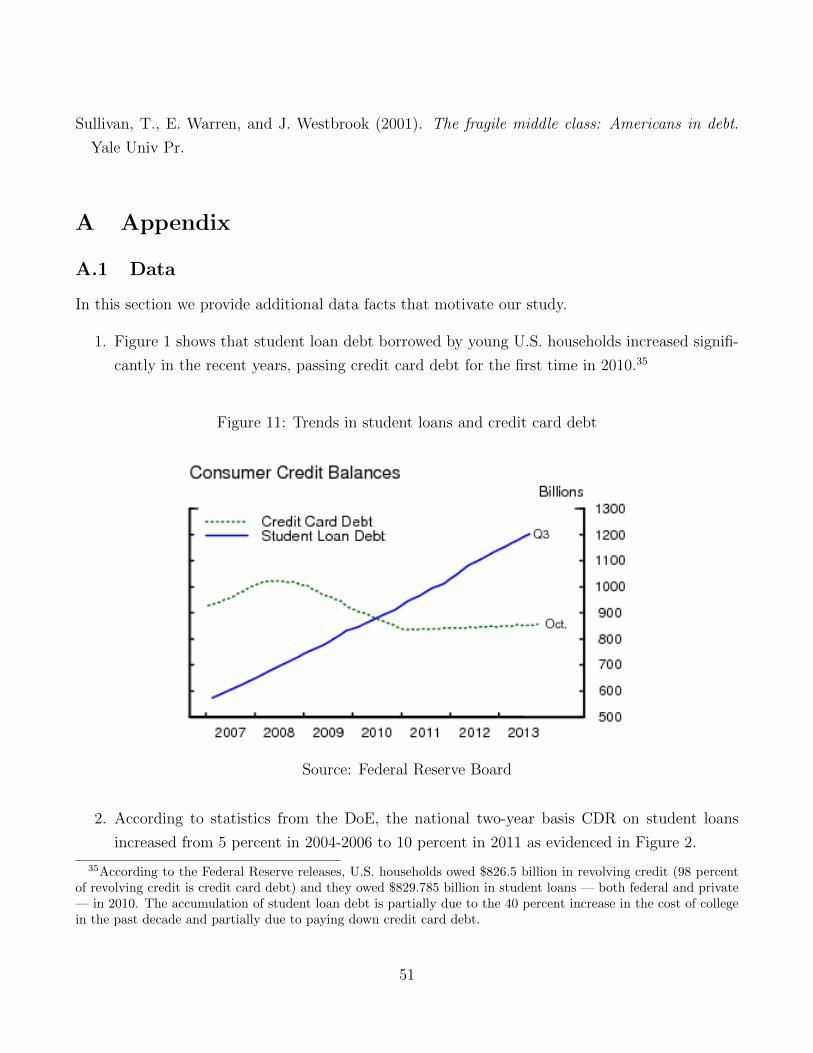
Sullivan, T., E. Warren, and J. Westbrook (2001). The fragile middle class: Americans in debt.

Yale Univ Pr.

A Appendix

A.1 Data

In this section we provide additional data facts that motivate our study.

1. Figure 1 shows that student loan debt borrowed by young U.S. households increased signifi-

cantly in the recent years, passing credit card debt for the first time in 2010.35

Figure 11: Trends in student loans and credit card debt

Source: Federal Reserve Board

2. According to statistics from the DoE, the national two-year basis CDR on student loans

increased from 5 percent in 2004-2006 to 10 percent in 2011 as evidenced in Figure 2.

35According to the Federal Reserve releases, U.S. households owed $826.5 billion in revolving credit (98 percentof revolving credit is credit card debt) and they owed $829.785 billion in student loans — both federal and private— in 2010. The accumulation of student loan debt is partially due to the 40 percent increase in the cost of collegein the past decade and partially due to paying down credit card debt.

51

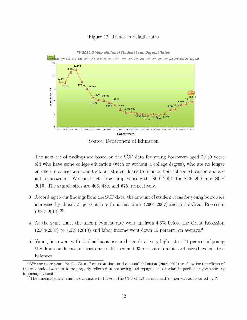
Figure 12: Trends in default rates

Source: Department of Education

The next set of findings are based on the SCF data for young borrowers aged 20-30 years

old who have some college education (with or without a college degree), who are no longer

enrolled in college and who took out student loans to finance their college education and are

not homeowners. We construct these samples using the SCF 2004, the SCF 2007 and SCF

2010. The sample sizes are 466, 430, and 675, respectively.

3. According to our findings from the SCF data, the amount of student loans for young borrowers

increased by almost 21 percent in both normal times (2004-2007) and in the Great Recession

(2007-2010).36

4. At the same time, the unemployment rate went up from 4.3% before the Great Recession

(2004-2007) to 7.6% (2010) and labor income went down 19 percent, on average.37

5. Young borrowers with student loans use credit cards at very high rates: 71 percent of young

U.S. households have at least one credit card and 93 percent of credit card users have positive

balances.

36We use more years for the Great Recession than in the actual definition (2008-2009) to allow for the effects ofthe economic downturn to be properly reflected in borrowing and repayment behavior, in particular given the lagin unemployment.

37The unemployment numbers compare to those in the CPS of 4.8 percent and 7.3 percent as reported by ?.

52

6. Terms on credit card accounts of young borrowers have changed: the credit card limit in-

creased by 30 percent from 2004 to 2007 but decreased by about the same percentage during

the Great Recession (2007-2010). The average amount lent by credit card issuers to young

borrowers declined by 31.5 percent from 2007 to 2010.38

A.2 Proofs of theorems

A.3 Proofs of Theorems 1 and 2

Let cmin = ymin(1− γ) and cmax = ymax + bmax − bmin. Then, if c is the consumption in any of the

cases in the definition of T , we have that U(cmin) ≤ U(c) ≤ U(cmax) and that cmin is a feasible

consumption. Recall that S = B × F ×H is a finite set and let NS be the cardinality of S.

Definition A1. Define V to be the set of continuous functions v : D × Y ×Q→ RNS such that

1. For all (b, f, h) ∈ S and (d, y, q) ∈ D × Y ×Q

U(cmin)

1− βρ≤ v(d, y, q)(b, f, h) ≤ U(cmax)

1− βρ. (3)

2. v is increasing in b and y.

3. v is decreasing in f : v(d, y, q)(b, 0, h) ≥ v(d, y, q)(b, 1, h) for all d, y, q, b, h.

Let(C(D × Y × Q;RNS ), ‖ · ‖

)denote the space of continuous functions v : D × Y × Q → RNS

endowed with the supremum norm

‖v‖ = max(d,y,q)

‖v(d, y, q)‖,

where the norm of a vector w = (w(b, f, h)) ∈ RNS is

‖w‖ = max(b,f,h)∈S

|w(b, f, h)|.

38In general, credit card terms deteriorated in the past several years: credit card providers have levied some of thelargest increases in interest rates, fees and minimum payments. For instance, JPMorgan Chase, the biggest creditcard provider, raised the minimum payment on outstanding balances from 2 percent to 5 percent for some customersand raised its balance-transfer fee from 3 percent to 5 percent – the highest rate among the large consumer banks(June 30 Bloomberg article). Citigroup has reportedly raised rates on outstanding balances by nearly 3 percentagepoints to an average of 24 percent for 13 million to 15 million cardholders (July 1 2009 Financial Times article).

53

Then V is a subset of C(D×Y ×Q;RNS ). Define also C(D×Y ×Q×S) to be the set of continuous

real valued functions v : D × Y ×Q× S → R with the norm

‖v‖ = max(d,y,q,b,f,h)

|v(d, y, q, b, f, h)|.

In the first lemma we show that the two spaces of functions that we defined above are interchange-

able.

Lemma A1. The map V : C(D × Y ×Q;RNS )→ C(D × Y ×Q× S) defined by

V (v)(d, y, q, b, f, h) = v(d, y, q)(b, f, h)

is a surjective isomorphism.

Proof. We prove first that if v ∈ C(D×Y×Q;RNS ) then V (v) is continuous. Let (dn, yn, qn, bn, fn, hn)n∈N

be a sequence that converges to (d, y, q, b, f, h) and let ε > 0. Since S is a finite set it follows that

there is some N1 ≥ 1 such that bn = b, fn = f , and hn = h for all n ≥ N1. Since v is continuous

then there is N2 ≥ 1 such that if n ≥ N2 then

‖v(dn, yn, qn)− v(d, y, q)‖ < ε.

Thus |v(dn, yn, qn)(b, f, h)− v(d, y, q)(b, f, h)| < ε for all n ≥ N := max{N1, N2}. Therefore

|V (v)(dn, yn, qn, bn, fn, hn)− V (v)(d, y, q, b, f, h)| < ε for all n ≥ N

and V (v) is continuous. It is clear from the definition of the norms that ‖V (v)‖ = ‖v‖ for all

v ∈ C(D × Y ×Q;RNS ). Thus V is an isomorphism. Finally, if w ∈ C(D × Y ×Q× S) then one

can define v ∈ C(D × Y ×Q;RNS ) by

v(d, y, q)(b, f, h) = w(d, y, q, b, f, h).

Then T (v) = w and T is surjective.

In the following we are going to tacitly view V either as a subset of C(D×Y ×Q;RNS ) or as a

subset of C(D×Y ×Q×S) via V (V). For example, we are going to prove in the following lemma

that (V , ‖ · ‖) is a complete metric space by showing that it(’s image under V ) is a closed subspace

of C(D × Y ×Q× S), which is a complete metric space.

Lemma A2. (V , ‖ · ‖) is a complete metric space.

54

Proof. We are going to show that V is a closed subspace of C(D×Y ×Q×S). Notice first that V is

nonempty because any constant function that satisfies (3) is in V . Let now {vn}n∈N be a sequence

of functions in V that converge to a function v. Then, since C(D×Y ×Q×S) is complete, it follows

that v is continuous. Since inequalities are preserved by taking limits it follows immediately that

v satisfies the conditions of Definition A1, because each vn satisfies those conditions. Therefore

v ∈ V and, thus, (V , ‖ · ‖) is a closed subspace of C(D×Y ×Q×S) and, hence, a complete metric

space.

Lemma A3. The operator T defined on C(D× Y ×Q;RNS ) maps V into V and its restriction to

V is a contraction with factor βρ.

Proof. We will show first that if v ∈ V then Tv ∈ V . Since v ∈ V we have that

U(cmin)

1− βγ≤ v(d, y′, q)(b′, f ′, h′) ≤ U(cmax)

1− βγ

for all (d, y′, q) ∈ D × Y ×Q and (b′, f ′, h′) ∈ S. Integrating with respect to y′ we obtain that

U(cmin)

1− βγ≤ˆv(b′,f ′,h′)(d, y

′; q)Φ(dy′) ≤ U(cmax)

1− βρ,

because´

Φ(dy′) = 1. Since U(cmin) ≤ U(c) ≤ U(cmax) for all c appearing in the definition of T ,

it follows that

U(c) + βρ

ˆv(b′,f ′,h′)(d, y

′; q)Φ(dy′) ≤ U(cmax) +βρU(cmax)

1− βρ=U(cmax)

1− βρ,

and, similarlyU(cmin)

1− βρ≤ U(c) + βρ

ˆv(b′,f ′,h′)(d, y

′; q)Φ(dy′).

Thus the condition (3) of Definition A1 is satisfied. To prove that Tv is increasing in b and

y and decreasing in f , note that the sets Bb,f,h(d, y, ; q) are increasing with respect to b and y,

and decreasing with respect to f . These facts coupled with the same properties for v (which are

preserved by the integration with respect to y′) imply that Tv satisfies the remaining conditions

from Definition A1, with the exception of the continuity, which we prove next.

Since B,F,H and D are finite spaces, it suffices to show that Tv is continuous with respect

to y and q. Since Q is compact and v is uniformly continuous with respect to q, it follows by a

simple ε− δ argument that the integral is continuous with respect q. Since U(·) is continuous with

respect to c and c is continuous with respect to d and y, it follows that T (v) is continuous.

55

Finally we prove that T is a contraction with factor βρ by showing that T satisfies Blackwell’s

conditions. For simplicity, we are going to view V one more time as a subset of C(D×Y ×Q×S).

Let v, w ∈ V such that v(d, y, q, b, f, h) ≤ w(d, y, q, b, f, h) for all (d, y, q, b, f, h) ∈ D× Y ×Q×S.

Then

βρ

ˆv(b′,f ′,h′)(d, y

′; q)Φ(dy′) ≤ βρ

ˆw(b′,f ′,h′)(d, y

′; q)Φ(dy′)

for all (d, y, q, b′, f ′, h′). This implies that Tv ≤ Tw. Next, if v ∈ V and a is a constant it follows

that

βρ

ˆ (v(b′,f ′,h′)(d, y

′; q) + a)Φ(dy′) = βρ

ˆv(b′,f ′,h′)(d, y

′; q)Φ(dy′) + βρa.

Thus T (v + a) = Tv + βρa. Therefore T is a contraction with factor βρ.

Theorem 1. There exists a unique v∗ ∈ V such that v∗ = Tv∗ and

1. v∗ is increasing in y and b.

2. Default decreases v∗.

3. The optimal policy correspondence implied by Tv∗ is compact-valued, upper hemi-continuous.

4. Default is strictly preferable to zero consumption and optimal consumption is always positive.

Proof. The first two parts follows from Definition A1 and Lemmas A2 and A3. The last part

follows from our assumptions on U . So we need only to prove the third part of the theorem. The

optimal policy correspondence is

Ξ(d,y,q,b,f,h) ={

(c, b′, h′, f ′, λd, λb) ∈ Bb,f,h(d, y; q) that attain v∗b,f,h(d, y, q)}.

For simplicity of our notation we will write x = (d, y, q, b, f, h). For a fixed x we need to show that

if Ξx is nonempty then it is compact. First notice that

Ξx ⊂ [cmin, cmax]×B ×H × F × {0, 1} × {0, 1}

and, thus, it is a bounded set. We need to prove that it is closed. Let {(cn, b′n, h′n, f ′n, λnd , λnb )}n∈Nbe a sequence in Ξx that converges to some

(c, b′, h′, f ′, λd, λb) ∈ [cmin, cmax]×B ×H × F × {0, 1} × {0, 1}.

Since B,F , and {0, 1} are finite sets it follows that there is some N ≥ 1 such that b′n = b′, h′n = h′,

56

f ′n = f ′, λnd = λd, and λnb = λb for all n ≥ N . Define

φ(c) = U(c) + βρ

ˆv(b′,f ′,h′)(d, y

′; q)Φ(dy′).

Then φ is continuous and, since φ(cn) = v∗(b,f,h)(d, y; q) for all n ≥ 1, we have that

φ(c) = limn→∞

φ(cn) = v∗(b,f,h)(d, y; q).

Thus (c, b′, h′, f ′, λd, λb) ∈ Ξx and Ξx is a closed and, hence, compact set.

To prove that Ξ is upper hemi-continuous consider x = (d, y, q, b, f, h) ∈ D × Y × Q × S and

let {xn} ∈ D × Y × Q × S, xn = (dn, yn, qn, bn, fn, hn) be a sequence that converges to x. Since

D, B, F , and H are finite sets it follows that there is N ≥ 1 such that if n ≥ N then dn = d,

bn = b, fn = f , and hn = h. Let zn = (cn, b′n, h

′n, f

′n, λ

nd , λ

nb ) ∈ Ξxn for all n ≥ N . We need to find

a convergent subsequence of {zn} whose limit point is in Ξx. Since B, H, F , and {0, 1} are finite

sets we can find a subsequence {znk} such that b′nk

= b′, h′nk= h′, f ′nk

= f ′, λnkd = λd, λ

nkb = λb for

some b′ ∈ B, h′ ∈ H, f ′ ∈ F, λd, λb ∈ {0, 1}. Since {cnk} ⊂ [cmin, cmax] which is a compact interval,

there must be a convergent subsequence, which we still label cnkfor simplicity. Let c = limk→∞ cnk

and let znk= (cnk

, b′, h′, f ′, λd, λb) for all k. Then {znk} is a subsequence of {zn} such that

limk→∞

znk= z := (c, b′, h′, f ′, λd, λb).

Moreover, since

φ(cnk) = v∗b,f,h(dnk

, ynk; qnk

) for all k

and since φ and v∗ are continuous functions it follows that

φ(c) = limk→∞

φ(cnk) = lim

k→∞v∗b,f,h(dnk

, ynk; qnk

) = v∗b,f,h(d, y; q).

Thus z ∈ Ξx and Ξ is an upper hemi-continuous correspondence.

Theorem 2. For any q ∈ Q and any measurable selection from the optimal policy correspondence

there exists a unique µq ∈M(x) such that Γqµq = µq.

Proof. The Measurable Selection Theorem implies that there exists an optimal policy rule that is

measurable in X × B(X) and, thus, T ∗q is well defined. We show first that T ∗q satisfies Doeblin’s

condition. It suffices to prove that TN∗q satisfies Doeblin’s condition (see Exercise 11.4g of Stockey,

Lucas, Prescott (1989)). If we let ϕ(Z) = TN∗q (y, d, b, f, h, Z) for any (y, d, b, f, h) ∈ X it follows

57

that if ε < 1/2 and ϕ(Z) < ε then 1− ε > 1/2 and

TN∗q (y, d, b, f, h, Z) < ε <1

2< 1− ε

for all (y, d, b, f, h) ∈ X. Thus Doeblin’s condition is satisfied.

Next, notice that if ϕ(Z) > 0 then TN∗q (y, d, b, f, h, Z) > 0 and, thus,

T ∗q (y, d, b, f, h, Z) = ρTS∗q (y, d, b, f, h, Z) + (1− ρ)TN∗q (y, d, b, f, h, Z) > 0.

Then Theorem 11.10 of Stockey, Lucas, Prescott (1989) implies the conclusion of the theorem.

A.4 Proofs of Theorems 3-8

Let (b, f, h) ∈ S and q ∈ Q be fixed. Before proving the theorem we will introduce some notation

which will ease the writing of our proofs. For y ∈ Y , d ∈ D we define the following maps:

ψnodef (y, d)(c, b′, f ′, h′, λd = 0, λb = 0) := U(c) + βρ

ˆvb′,f ′,h′(d, y

′; q)Φ(dy′)

for all (c, b′, f ′, h′, 0, 0) ∈ Bb,f,h(d, y; q);

ψsl(y, d)(c, b′, f ′, h′, λd = 1, λb = 0) = U(c) + βρ

ˆvb′,f ′,1(d, y

′; q)Φ(dy′)

for all (c, b′, f ′, h′, 1, 0) ∈ Bb,f,h(d, y; q);

ψcc(y, d)(c, b′, f ′, h′, λd = 0, λb = 1) = U(c) + βρ

ˆvb′,1,h′(d, y

′; q)Φ(dy′)

for all (c, b′, f ′, h′, 0, 1) ∈ Bb,f,h(d, y; q); and

ψboth(y, d)(c, b′, f ′, h′, λd = 1, λb = 1) = U(c) + βρ

ˆv0,1,1(d, y

′; q)Φ(dy′)

for all (c, b′, f ′, h′, 0, 1) ∈ Bb,f,h(d, y; q). Note that these functions are continuous in y and d. Also,

these functions depend on b, f , and q. Also, we will write ωb,f,h(q, d) for the expected utility of an

household that starts next period with (b, f, h, q, d).

Theorem 3. Let q ∈ Q, f ∈ F , b ∈ B(f). If h = 1 and the set DSLb,f,1(q) is nonempty, then

DSLb,f,1(q) is closed and convex. In particular the sets DSL

b,f,1(d; q) are closed intervals for all d. If

h = 0 and the set DSLb,f,0(d; q) is nonempty, then DSL

b,f,0(d; q) is a closed interval for all d.

58

Proof. If h = 1 then DSLb,f,1(q) is the combinations of earnings y and student loan amount d for

which Bb,f,1(d, y; q) = ∅. Then they satisfy the inequality y(1− γ) + b(1− λb)− d− qb′,d,hb′ ≤ 0 for

all λb ∈ {0, 1} and b′ ∈ B . Thus DSLb,f,1(q) is closed. Moreover, if (y1, d1) and (y2, d2) are elements

in DSLb,f,1(q) then if (y, d) = t(y1, d1) + (1− t)(y2, d2) with t ∈ (0, 1) it follows easily that

y(1− γ) + b(1− λb)− d− qb′,d,hb′ ≤ 0

and, thus, (y, d) ∈ DSLb,f,1(q). So DSL

b,f,1(q) is convex.

Assume now that h = 0 and let d ∈ D be fixed. Let y1 and y2 with y1 < y2 be in DSLb,f,0(d; q).

Therefore

ψsl(yi, d)(c∗i , b′∗i , f

′∗i , h

′∗i , 1, 0) ≥ max

{ψnodef (yi, d)(c, b′, f ′, h′, 0, 0), (4)

ψcc(yi, d)(c, b′, h′, 0, 1),

ψboth(y, d)(c, b′, h′, 1, 1)}

for all (c, b′, f ′, h′, 0, 0), (c, b′, f ′, h′, 0, 1), (c, b′, f ′, h′, 1, 1) ∈ Bb,f,0(d, yi; q), i = 1, 2. Let y ∈ (y1, y2)

and assume, by contradiction, that y /∈ DSLb,f,0(d; q). Assume, without loss of generality, that the

agent chooses not to default on either market, i.e.

ψsl(y, d)(c, b′, f ′, h′, 1, 0) < ψnodef (y, d)(c∗, b′∗, f ′∗, h′∗, 0, 0), (5)

for all (c, b′, f ′, h′, 1, 0) ∈ Bb,f,0(d, y; q), where (c∗, b′∗, f ′∗, h′∗, 0, 0) ∈ Bb,f,0(d, y; q) is the optimal

choice for the maximization problem. Let c1 = c∗ − (y − y1). If c1 ≤ 0 then c1 < y1 + b and thus

c∗ = c1 + (y − y1) < y1 + b+ (y − y1) = y + b. (6)

If c1 > 0 we have that (c1, b′∗, f ′∗, h′∗, 0, 0) ∈ Bb,f,0(d, y1; q) and, thus,

ψsl(y1, d)(c∗1, b′∗1 , f

′∗1 , h

′∗i , 1, 0) ≥ ψnodef (y1, d)(c, b′∗, f ′∗, h′∗, 0, 0).

Therefore

U(y1 + b) + βρ

ˆvb′∗1 ,f ′∗1 ,1(d, y

′; q)Φ(dy′) ≥ U(c1) + βρ

ˆvb′∗,f ′∗,0(d, y

′; q)Φ(dy′), (7)

59

Subtracting (7) from (5) we have that

U(y + b)− U(y1 + b) < U(c∗)− U(c1).

Since (y + b)− (y1 + b) = y − y1 = c∗ − c1 and U is strictly concave it follows that c∗ < y + b.

Consider now c2 = c∗ + (y2 − y). Then (c2, b′∗, f ′∗, h′∗, 0, 0) ∈ Bb,f,0(d, y2; q) and thus

U(y2 + b) + βρ

ˆvb′∗2 ,f ′∗2 ,1

(d, y′; q)Φ(dy′) ≥ U(c2) + βρ

ˆvb∗,f∗,0(d, y

′; q)Φ(dy′). (8)

Using inequalities (5), and (8) we obtain that

U(y2 + b)− U(y + b) > U(c2)− U(c∗).

Thus c∗ > y + b, and we obtain a contradiction with c∗ < y + b. Therefore y ∈ DSLb,f,0(d; q) and,

thus, DSLb,f,0(d; q) is an interval. It is also a closed set because the maps ψsl, ψboth, ψcc, and ψnodef

are continuous with respect to y. Thus, DSLb,f,0(d; q) is a closed interval.

Theorem 4. Let q ∈ Q, (b, f, 0) ∈ S. If DCCb,f,0(d; q) is nonempty then it is a closed interval for all

d.

Proof. If b ≥ 0 then DCCb,f,0(d; q) is empty. If b < 0 the proof of the theorem is very similar with the

proof of Theorem 3 and we will omit it.

Theorem 5. Let q ∈ Q, (b, f, 0) ∈ S. If the set DBothb,f,0 (d; q) is nonempty then it is a closed

interval for all d.

Proof. If b ≥ 0 then the set DBothb,f,0 (d; q) is empty. For b < 0 the proof is similar with the proof of

Theorem 3.

Theorem 6. For any price q ∈ Q, d ∈ D, f ∈ F , and h ∈ H, the sets DCCb,f,h(d; q) expand when b

decreases.

Proof. Let b1 > b2. Then

{(c, b′, f ′, h′, 0, 1) ∈ Bb1,f,h(d, y; q)

}=

{(c, b′, f ′, h′, 0, 1) ∈ Bb2,f,h(d, y; q)

},{

(c, b′, f ′, h′, 1, 1) ∈ Bb1,f,h(d, y; q)}

={

(c, b′, f ′, h′, 1, 1) ∈ Bb2,f,h(d, y; q)},{

(c, b′, f ′, h′, 0, 0) ∈ Bb1,f,h(d, y; q)}⊇

{(c, b′, f ′, h′, 0, 0) ∈ Bb2,f,h(d, y; q)

},{

(c, b′, f ′, h′, 1, 0) ∈ Bb1,f,h(d, y; q)}⊇

{(c, b′, f ′, h′, 1, 0) ∈ Bb2,f,h(d, y; q)

}.

60

Thus, if for b1,

ψcc(y, d)(c∗, b′∗, f ′∗, h′∗, 0, 1) ≥ max{ψnodef (y, d)(c, b′, f ′, h′, 0, 0),

ψsl(y, d)(c, b′, h′, 1, 0),

ψboth(y, d)(c, b′, h′, 1, 1)},

it follows that the same inequality will hold for b2 as well. Therefore, DCCb1,f,h

(d; q) ⊆ DCCb2,f,h

(d; q).

Theorem 7. For any price q ∈ Q, b ∈ B, f ∈ F , and h ∈ H, the sets DCCb,f,h(d; q) shrink and

DBothb,f,h (d; q) expand when d increases.

Proof. Let d1 < d2. Then

{(c, b′, f ′, h′, 0, 1) ∈ Bb,f,h(d1, y; q)

}⊇

{(c, b′, f ′, h′, 0, 1) ∈ Bb,f,h(d2, y; q)

},{

(c, b′, f ′, h′, 1, 1) ∈ Bb,f,h(d1, y; q)}

={

(c, b′, f ′, h′, 1, 1) ∈ Bb,f,h(d2, y; q)},{

(c, b′, f ′, h′, 0, 0) ∈ Bb,f,h(d1, y; q)}⊇

{(c, b′, f ′, h′, 0, 0) ∈ Bb,f,h(d2, y; q)

},{

(c, b′, f ′, h′, 1, 0) ∈ Bb,f,h(d1, y; q)}

={

(c, b′, f ′, h′, 1, 0) ∈ Bb,f,h(d2, y; q)}.

Thus, if

ψboth(y, d1)(c∗, b′∗, f ′∗, h′∗, 1, 1) ≥ max

{ψnodef (y, d1)(c, b

′, f ′, h′, 0, 0),

ψsl(y, d1)(c, b′, h′, 1, 0),

ψcc(y, d1)(c, b′, h′, 0, 1)

},

it follows that the same inequality holds for d2. Therefore, DBothb,f,h (d1; q) ⊆ DBoth

b,f,h (d2; q). On the

other hand, if

ψcc(y, d1)(c∗, b′∗, f ′∗, h′∗, 0, 1) ≥ max

{ψnodef (y, d1)(c, b

′, f ′, h′, 0, 0),

ψsl(y, d1)(c, b′, h′, 1, 0),

ψboth(y, d1)(c, b′, h′, 1, 1)

},

the inequalities can reverse for d2. Therefore DCCb,f,h(d1; q) ⊇ DCC

b,f,h(d2; q).

Theorem 8. For any price q ∈ Q, b ∈ B, d ∈ D, and f ∈ F , the set DCCb,f,0(d; q) ⊂ DCC

b,f,1(d; q).

Proof. Let y ∈ Y . For h = 1 we have that

{(c, b′, f ′, h′, 1, 1) ∈ Bb,f,1(d, y; q)

}= ∅

61

and {(c, b′, f ′, h′, 1, 0) ∈ Bb,f,1(d, y; q)

}= ∅.

Therefore, if for f = 0 we have that

ψcc(y, d1)(c∗, b′∗, f ′∗, h′∗, 0, 1) ≥ max

{ψnodef (y, d1)(c, b

′, f ′, h′, 0, 0),

ψsl(y, d1)(c, b′, h′, 1, 0),

ψboth(y, d1)(c, b′, h′, 1, 1)

},

then the same inequalities hold for f = 1.

A.5 Proofs of Theorems 9 and 10

Theorem 9. Existence A steady-state competitive equilibrium exists.

We see that once q∗ is known, then all the other components of the equilibrium are given by the

formulas in Definition 2. We can rewrite part 5 of the Definition as

q∗d,h,b′ =ρ

1 + r(1− pbd,h,b′)

=ρ

1 + r

(1−ˆλ∗b(y

′, d, 0, b′, h′, q∗)φ(dy′)H∗(h, dh′)

),

where λ∗b and f ′∗ are measurable selections guaranteed by Theorem 1, and H∗ is the transition

matrix provided by Theorem 1. Thus q∗ is a fixed point of the map T : [0, qmax]ND×NH×NB 7→

[0, qmax]ND×NH×NB

T (q)(d, h, b′) =ρ

1 + r

(1−ˆλ∗b(y

′, d, 0, b′, h′, q)φ(dy′)H∗(h, dh′)

). (9)

Since Q := [0, qmax]ND×NH×NB is a compact convex subset of RND×NH×NB we can apply the Schauder

theorem (Theorem V.19 of ?) if we prove that the map

q 7→ˆλ∗b(y

′, d, 0, b′, h′, q)φ(dy′)H∗(h, dh′)

is continuous.

Before starting the proof we remark that the above map is well defined because even though

apriori the transition matrix H∗ depends on (y, d, b, f, q), in fact, knowing the pair (h, b′) completely

determines H∗(h, dh′) when b′ < 0. If b′ < 0 then f = 0, λ∗d = 0. Thus H∗(0, 0) = 1, H∗(0, 1) = 0,

62

H∗(1, 0) = ph and H∗(1, 1) = 1− ph. Also, if b′ ≥ 0 then pbd,h,b′ = 0 by definition.

We begin by showing that the sets of discontinuities of λ∗b(·, q) and b∗(·, q) , q ∈ Q, and λ∗b(x, ·)and b∗(x, ·), x ∈ X, have measure 0. This will follow from the following lemmas. Let us begin by

noticing that the sets of discontinuities of these functions are contained in the sets of indifference.

We fix b ∈ B, f ∈ F , h ∈ H, d ∈ D, and q ∈ Q and we will suppress the dependence of

functions on these variables. That is, we study the behavior with respect to y. Since B,F,H, and

D are finite sets this will suffice to prove the continuity of λ∗b(·, q). The first step is to study in

more detail the maximization problem on the no default path. Recall that

ψnodef (y, d)(c, b′, f ′, h′, 0, 0) = U(c) + βρ

ˆvb′,0,0(d, y

′; q)Φ(dy′)

for all (c, b′, 0, 0, 0, 0) ∈ Bb,f,h(d, y; q). For y ∈ Y we write b′(y) for the the values of b′ that

maximize ψnodef . Recall that b, f, h, d, and q are fixed and that b′(y) can be a correspondence.

Since t is a lump sum tax that is paid by every agent in the economy, it does not affect the choices.

For simplicity we assume that t = 0 in the following.

Lemma A4. Let b ∈ B, f ∈ F , h ∈ H, d ∈ D, and q ∈ Q be fixed. Then for any y0 ∈ Y there is

ε > 0 such that the following holds:

1. If b′(y0) is a single valued then b′ is constant and single valued on (y0 − ε, y0 + ε).

2. If b′(y0) is multi-valued then either b′(y) is single valued on (y0 − ε, y0 + ε) \ {y0} and there

is b̄ ∈ b′(y0) such that b′(y) = b̄ for all y ∈ (y0 − ε, y0 + ε) \ {y0}, or b′(y) = b′(y0) for all

y ∈ (y0 − ε, y0 + ε) .

Proof. If b′(y0) is single valued, then

U(y0 + b− d− qd,h,b′(y0)b′(y0)) + βρ

ˆvb′(y0),0,0,(d, y

′; q)Φ(dy′) > (10)

U(y0 + b− d− qd,h,b′b′) + βρ

ˆvb′,0,0(d, y

′; q)Φ(dy′),

for all b′ ∈ B \ {b′(y0)} (the right hand side is −∞ if (c, b′, 0, 0, 0, 0) /∈ Bb,f,h(y0, d; q), where, here,

c = y0 + b− d− qd,h,b′b′). Then, since B(f) is finite and U is continuous with respect to y, we can

find ε > 0 such that if |y − y0| < ε then

U(y + b− d− qd,h,b′(y0)b′(y0)) + βρ

ˆvb′(y0),0,0(d, y

′; q)Φ(dy′) > (11)

U(y + b− d− qd,h,b′b′) + βρ

ˆvb′,0,0(d, y

′; q)Φ(dy′),

63

for all b ∈ B(f) \ {b′(y0)}. Thus b′(y) = b′(y0) for all |y − y0| < ε.

Suppose now that b′(y0) is multi-valued. WLOG, assume that b′(y0) consists of two elements

b′1 and b′2 (we can assume this since B is finite). Then

U(y0 + b− d− qd,h,b′1b′1) + βρ

ˆvb′1,0,0(d, y

′; q)Φ(dy′) =

U(y0 + b− d− qd,h,b′2b′2) + βρ

ˆvb′2,0,0(d, y

′; q)Φ(dy′)

and they both satisfy inequality (10) for all b′ ∈ B\{b′1, b′2}. There is ε > 0 such that if |y−y0| < ε,

then (11) is satisfied for both b′1 and b′2. We need to compare, thus, U(y + b − d − qd,h,b′1b′1) +

βρ´vb′1,0,0(d, y

′; q)Φ(dy′) and U(y+b−d−qd,h,b′2b′2)+βρ

´vb′2,0,0(d, y

′; q)Φ(dy′). If qd,h,b′1b′1 = qd,h,b′2b

′2,

then it follows that´vb′1,0,0(d, y

′; q)Φ(dy′) =´vb′2,0,0(d, y

′; q)Φ(dy′). Therefore

U(y + b− d− qd,h,b′1b′1) + βρ

ˆvb′1,0,0(d, y

′; q)Φ(dy′) =

U(y + b− d− qd,h,b′2b′2) + βρ

ˆvb′2,0,0(d, y

′; q)Φ(dy′)

for all y. Thus b′(y) = b′(y0) for all y ∈ (y0− ε, y0 + ε). Suppose now that qd,h,b′!b′1 < qd,h,b′2b

′2. Then

s0 := y0 + b− d− qd,h,b′1b′1 > y0 + b− d− qd,h,b′2b

′2 =: t0.

Assume that ε is so that t0+ε < s0−ε. Then, if |y−y0| < ε we have that t0 < y+b−d−qd,h,b′1b′1 =: s1,

t1 := y + b− d− qd,h,b′2b′2 < s0, and t1 < s1. Then we have

U(t1) + βρ

ˆvb′2,0,0(d, y

′; q)Φ(dy′) = U(t1)− U(t0) + U(t0) + βρ

ˆvb′2,0,0(d, y

′; q)Φ(dy′)

= U(t1)− U(t0) + U(s0) + βρ

ˆvb′1,0,0(d, y

′; q)Φ(dy′)

= U(t1)− U(t0) + U(s0)− U(s1)

+ U(s1) + βρ

ˆvb′1,f ′,0(d, y

′; q)Φ(dy′).

Since U is strictly concave, t0 < s0, t0 < s1, t1 < s1, t1 < s0, and t1 − t0 = s1 − s0 = y − y0, it

follows that U(t1)− U(t0) > U(s1)− U(s0). Thus

U(t1) + βρ

ˆvb′2,f ′,0(d, y

′; q)Φ(dy′) > U(s1) + βρ

ˆvb′1,f ′,0(d, y

′; q)Φ(dy′)

64

and b′2 is the only solution to the maximization problem. Therefore b′ is single valued and equals

b′2 on (y0 − ε, y0 + ε) \ {y0}. The case qd,h,b′b′1 > qd,h,b′2b

′2 is similar.

Lemma A5. Let b ∈ B, f ∈ F , h ∈ H, d ∈ D, and q ∈ Q be fixed. Suppose that y1 is a point

of indifference between not defaulting and defaulting on student loans. Then, if ε is small enough,

either there is no other point y of indifference with |y− y1| < ε or all y ∈ (y1− ε, y1 + ε) are points

of indifference.

Proof. Let ε > 0 be such that for all y ∈ Y with |y − y1| < ε we have that b′(y) = b′(y1) =: b′.

We can find such an ε by Lemma (A4): if b′(y1) is single-valued, then this is the first part of the

lemma; if b′(y1) is multi-valued, the second part of the lemma implies that we can pick b̄ ∈ b′(y1)such that b̄ ∈ b′(y) or b′(y) = b̄ for all y ∈ (y1 − ε, y1 + ε). We will consider b′(y) = b̄ in both cases

(note that this choice does not alter the measurability of b′∗). Assume first that d 6= qd,h,b′b′, which

implies that c1 6= y1 + b, and assume, by contradiction, that y2 is another point of indifference and

the distance between y1 and y2 is smaller than ε. Then

U(c1) + βρ

ˆvb′,0,0(d, y

′; q)Φ(dy′) = U(y1 + b) + βρ

ˆv0,0,1(d, y

′; q)Φ(dy′)

and

U(c2) + βρ

ˆvb′,0,0(d, y

′; q)Φ(dy′) = U(y2 + b) + βρ

ˆv0,0,1(d, y

′; q)Φ(dy′).

Therefore U(c1)− U(c2) = U(y1 + b)− U(y2 + b). However, we have that

c1 − c2 = y1 − y2 = (y1 + b)− (y2 + b).

This is a contradiction with U being strictly concave. If d = qd,h,b′b′ then c1 = y1 + b, and, hence,

c = y + b for all y, then all points y with |y − y1| < ε are indifference points.

The above lemma holds also for for all types of indifference. Thus, since Y is compact, if we

fix d and q, there are only a finite number of earning levels that are discontinuity points for λ∗d, λ∗b ,

and b∗.

Lemma A6. The set of pairs {y, d} that are points of discontinuity for λ∗d, λ∗b , and b∗ has measure

0.

Proof. Lemma A5 implies that we can change the maps in a Borel way so that for each d ∈ D the

set of y ∈ Y for which these maps are discontinuous is finite. The conclusion follows now since D

is finite.

65

Proof. of Theorem 9 Let {qn}n∈N ⊂ Q be a sequence that converges to q. We will show that

limn→∞ λ∗b(y, d, f, b, h, qn) = λ∗b(y, d, f, b, h, q) almost everywhere. Since the sequence {qn} is count-

able, by Lemma A5 we can find a set E ⊂ X of measure 0 that contains all the points of indifference

for the prices qn, n ∈ N, and q. Let (y, d, f, b, h) ∈ X \E be fixed. Since vb,f,h(d, y; ·) is continuous

and Q is a compact space it follows that vb,f,h(d, y; ·) is uniformly continuous. Therefore, since B

is finite, there is δ > 0 such that if ‖q′ − q′′‖ < δ and

ψnodef (q′)(c∗, b∗, f ′, h′, 0, 0) > max

{max

(c,b′,f ′,h′,1,0)ψsl(q

′)(c, b′, f ′, h′, 1, 0),

max(c,b′,f ′,h′,0,1)

ψcc(q′)(c, b′, f ′, h′, 0, 1),

max(c,b′,f ′,h′,1,1)

ψboth(q′)(c, b′, f ′, h′, 1, 1)

}then the same inequality holds for q′′. In the inequality above we suppressed the dependence on

(y, d, f, b, h) to simplify the notation. Thus, if λ∗b(y, d, f, b, h, q′) = 0 and λ∗d(y, d, f, b, h, q

′) = 0

then λ∗b(y, d, f, b, h, q′′) = 0 and λ∗d(y, d, f, b, h, q

′′) = 0. Similar statements hold for all possible

combinations of values of λ∗b and λ∗d. Therefore, by shrinking δ if necessary, we have that if ‖q′ −q′′‖ < δ then λ∗b(y, d, f, b, h, q

′) = λ∗b(y, d, f, b, h, q′′). This implies that limn→∞ λ

∗b(y, d, f, b, h, qn) =

λ∗b(y, d, f, b, h, q) for all (y, d, f, b, h, q) ∈ X \ E. Finally, since |λ∗b(y, d, f, b, h, q)| ≤ 1 and X is a

compact space, the Lebesgue’s Dominated Convergence Theorem (see, for example, (?, Theorem

1.34)) implies that

limn→∞

ˆλ∗b(y

′, d, f ′, b′, h′, qn)Φ(dy)H(h, dh′) =

ˆλ∗b(y

′, d, f ′, b′, h′, qn)Φ(dy)H(h, dh′).

Thus the map T defined in (9) is continuous and, hence, has a fixed point.

Theorem 10. In any steady-state equilibrium the following is true:

1. For any b′ ≥ 0, q∗d,h,b′ = ρ/(1 + r) for all d ∈ D and h ∈ H.

2. If the grids of D and B are sufficiently fine, and h = 0 there are d > 0 and b′ < 0 such that

q∗d,h,b′ = ρ/(1 + r) for all d < d and b′> b′.

3. If the set of income levels for which the household is indifferent between defaulting on credit

card debt and any other available option is of measure zero, then d1 < d2 implies q∗d1,h,b′ >

q∗d2,h,b′ for any h ∈ H and b′ ∈ B.

4. If the set of income levels for which the household is indifferent between defaulting on credit

66

card debt and any other available option is of measure zero, then q∗d,h=1,b′ > q∗d,h=0,b′ for any

d ∈ D and b′ ∈ B.

Proof. The first part follows from part 5) of the definition of an equilibrium.

For the second part, assume that there are b1 < 0 and d > 0 such that y + b1 − d1 > 0 for all

y ∈ Y and consider any household with b1 < b < 0 and 0 < d < d. In particular the household

must have a clean default flag on the credit card market and on the student loan market. If an

household with debt b < 0 defaults only on the credit card market then its utility is

u(y − d)− τb + βρ

ˆu(y′ − d− q∗b′∗(d,y′;q)(b,0,0),d,0b′∗(d, y′; q)(b, 0, 0)

)Φ(dy′)

+ (βρ)2ˆ

(1− pf )ωb′∗(d,y′;q)(b,0,0),1,0(q∗, d) + pfωb′∗(d,y′;q)(b,0,0),0,0(q∗, d)Φ(dy′).

On the other hand, one feasible action of the household is to not default on any market, pay off

the debt and save in the following period b′∗(d, y′; q)(b, 0, 0). The utility from this course of action

is

u(y + b− d) + βρ

ˆu(y′ − d− q∗b′∗(d,y′;q)(b,0,0),d,0b′∗(d, y′; q)(b, 0, 0)

)Φ(dy′)

+ (βρ)2ˆωb′∗(d,y′;q)(b,0,0),0,0(q

∗, d)Φ(dy′).

Then property 3) of Definition A1 implies that the utility gain by not defaulting is at least

u(y + b− d)− u(y − d) + τb.

Assuming that the grid of B is sufficiently fine so that we can find b > b1 such that the above

expression is positive for all b > b and d < d the conclusion follows. The proof for the case when

the household defaults on both markets is similar.

Assuming that the set of income levels for which the household is indifferent between defaulting

on credit card debt and any other available option, Theorem 7 implies that if d1 < d2 then

pb∗d1,h,b′ ≤ pb∗d2,h,b′ for any h ∈ H and b′ ∈ B. The third part of the theorem follows. One can

similarly prove the last part of the theorem.

A.6 Proof of Theorem 11

Theorem 11. If the grids of D and B are fine enough, then we can find d1 ∈ D and b1 ∈ B such

that the agent defaults. Moreover, we can find d2 ≥ d1 and b2 ≤ b1 such that the agent defaults on

67

student loans.

Proof. Suppose that D is fine enough so that we can find d1 > 0 such that given A > 1 to be

specified below we have that |u′(y − d1)| ≥ A for all y ∈ Y such that y > d1. Since qmax < 1 then

we can find b1 < 0 such that b− qmaxb′ < 0 for all b′ ∈ B. The utility from defaulting on the credit

card for b1 is

u(y − d1)− τb + βρω0,1,0(q∗, d1)

and the utility from not defaulting on either path is

u(y + b1 − d1 − qb′∗(d,y;q)(b,f,h),d1,hb′∗(d, y; q)(b, f, h)) + βρωb′∗(d,y;q)(b,f,h),d1,h(q∗, d1).

Using the mean value theorem we can find c′ such that y+b1−d1−cb′∗(d,y;q)(b,f,h),d1,hb′∗(d, y; q)(b, f, h) <

c′ < y − d1 and

u(y−d1)−u(y+b1−d1−qb′∗(d,y;q)(b,f,h),d1,hb′∗(d, y; q)(b, f, h)) = u′(c′)(b1−qb′∗(d,y;q)(b,f,h),d1,hb′∗(d, y; q)(b, f, h)).

In particular, |u′(c′)| > A. We chose A such that

A(qb′b′ − b1) > τb + βρ(ωb′∗(d,y;q)(b,f,h),d1,h(q

∗, d1)− ω0,1,0(q∗, d1)),

for all b′ ∈ B. It follows that the utility from defaulting on credit card is higher than the utility of

not defaulting at all.

Suppose now that the grids of D and B are fine enough so that we can find d2 and b′2 such that

u(y + b′2)− u(y − d2)− τd + τb is zero or as close to zero as we want. That is, the agent’s current

utility from defaulting on student loans or credit card are basically the same. Then, if an agent

chooses to default on the credit card market today, in the next period her utility will be

u(y′ − d2 − qd2,0,b”∗CCb”∗CC) + βρ

((1− pf )ωb”∗CC ,0,1

(d2, q∗) + pfωb”∗CC ,0,0

(d2, q∗)),

where b”∗CC ≥ 0. If the agent chooses to default on student loans, she can chose to borrow b”2 < 0

such that y′(1− γ)− d2 − qb”2b”2 > y′ − d2 − qd2,0,b”∗CC

b”∗CC and |u′(y′(1− γ)− d2 − qb”2b”2)| > B, where

B is so that

u′(c′)(−γy′ − qb”2b”2 + qd2,0,b”∗CC

b”∗CC) ≥ (1− ph)ωb”2,0,1(d2, q∗) + phωb”2,0,0(d2, q

∗)

−((1− pf )ωb”∗CC ,0,1

(d2, q∗) + pfωb”∗CC ,0,0

(d2, q∗)).

68

Thus, if b2 = min{b′2, b′′2} it follows that the agent chooses to default on student loans.

69