HAL Id: hal-01941338https://hal.archives-ouvertes.fr/hal-01941338

Submitted on 30 Nov 2018

HAL is a multi-disciplinary open accessarchive for the deposit and dissemination of sci-entific research documents, whether they are pub-lished or not. The documents may come fromteaching and research institutions in France orabroad, or from public or private research centers.

L’archive ouverte pluridisciplinaire HAL, estdestinée au dépôt et à la diffusion de documentsscientifiques de niveau recherche, publiés ou non,émanant des établissements d’enseignement et derecherche français ou étrangers, des laboratoirespublics ou privés.

The interface between mathematics and engineering –problem solving processes for an exercise on oscillating

circuits using ordinary differential equationsJörg Kortemeyer, Rolf Biehler

To cite this version:Jörg Kortemeyer, Rolf Biehler. The interface between mathematics and engineering – problem solvingprocesses for an exercise on oscillating circuits using ordinary differential equations. CERME 10, Feb2017, Dublin, Ireland. �hal-01941338�

The interface between mathematics and engineering – problem solving

processes for an exercise on oscillating circuits using ordinary

differential equations

Jörg Kortemeyer and Rolf Biehler

University of Paderborn, Germany; kortemey@math.upb.de, biehler@math.upb.de

In our project, we investigate the mathematical skills that are required in first-year courses of

technical subjects of engineering bachelor courses, i.e., we do not look at the courses on pure math.

We analyze four exercises from an exam in electrical engineering, which is compulsory for first-

years. To solve such exercises, students have to combine their knowledge in electrical engineering

with their skills in mathematics. We introduce a theoretical approach consisting of three elements:

a normative solution called “student-expert-solution, “low-inferent analyses” for qualitative

studies with students, and categorizations of written solutions. We describe the newly developed

tools and details on one of the exercises and present the results from the analysis of the exercise in

reference to the three concepts mentioned above. This provides insight into the interface between

mathematics and engineering courses in the first year at university.

Keywords: Engineering mathematics, competence, differential equations.

Introduction

Engineering students at German universities are taught mathematical subjects as well as engineering

subjects, which require some understanding of mathematical topics, at the same time. This leads to

several challenges for the students: To begin with, the lectures on Mathematics for Engineering

Students (MfES) and the Fundamentals of Engineering (FoE) are very often asynchronous. On the

one hand, there is a deductive structure in the lectures on mathematics, which leads to a certain

order of presentation of the different topics to assure understanding. On the other hand, there is also

a standard way of presentation of the different engineering topics in the FoE-courses and because of

that, mathematical topics are often needed earlier in the FoE-courses than they are presented in the

MfES-courses. Moreover, there are different mathematical practices in MfES and FoE, for example

in the use of vectors or differentials (see e. g. Alpers, 2015). There is a mismatch between the

mathematics in MfES-courses, the mathematics at school level, and the “contextual mathematics”

required in engineering tasks (see e. g. Redish, 2005).

At the beginning of the research, our central question was: how do engineering students solve tasks

in basic engineering courses given this situation with two interconnected fields of competences -

mathematics and engineering. We are interested in the modelling and assessing of explicit as well as

implicit competences required and developed by students in this field. We investigate how students

actually solve exercises in FoE-courses and which difficulties occur. Our focus is on four typical

exercises of a FoE-exam after the first year at university. In this paper, we present a case study of

these issues in the context of a single exercise on ordinary differential equations in the electrical

engineering field of oscillating circuits. Our focus here is on the following research questions:

1. What are the expectations from students’ solutions to an exercise on ordinary differential

equations in a first-year electrical engineering course? 2. What are the characteristics of students’

problem-solving processes (e. g. strategies, difficulties) in electrical engineering courses?

For the analysis of students’ work we required a normative solution of the exercise, which was

developed with engineering experts and which considers both fields of competences. This

normative solution is based on relevant theoretical concepts that are presented in the next section.

Theoretical background

In this section, we present the theoretical tools that were used to develop the newly constructed

methodology for our investigations. As a first step, the approaches deal with modelling processes

using mathematical methods and mathematical problem solving. Both theoretical approaches are

relevant, as they combine inner- and outer-mathematical solution parts and describe their

connections. Next, we also consider actual solving processes that help us to supplement normative

solutions with the steps students use when solving an exercise.

The first approach is the modelling cycle by Blum and Leiss (2007), which is used to describe

idealized modelling processes of real world problems that can be solved using mathematics. In a

broad outline, it divides the modelling processes into two distinct parts, the so-called “rest of the

world” and “mathematics”. Our second perspective is mathematical problem solving by Polya

(1949), who intended to give advice to students on how to solve mathematical problems as well as

applied problems referring to mathematics. He divides the solving processes into four phases:

understanding the problem, devising a plan, carrying out the plan, and looking back.

For the analysis of actual solution processes of students, we use theoretical approaches developed by

Redish and his working group, i.e., by Redish and Tuminaro (2007) and Redish and Bing (2008), in

addition to the normative solution. Their approaches discuss the role of mathematical resources and

knowledge in solving processes by pairs of physics students. Redish and Tuminaro (2007)

distinguish three framings in qualitative solving processes: quantitative sense-making, qualitative

sense-making, and rote equation chasing (without understanding the underlying physical situation).

Bing (2008) looked at mathematical justification strategies and found four distinct types of

justifications: calculation (a correctly done algorithm gives a correct result), physical mapping (the

physical behavior is described correctly by mathematical results), invoking authority (the result is

consistent with the lecture) and math consistency (the same mathematical approach is used in a

similar situation). The theoretical background is presented in more detail in Biehler, Kortemeyer,

and Schaper (2015).

The newly developed methodology and its aims

In order to do research in this interface of two interconnected competence fields, new theoretical

approaches had to be developed. This section presents the three main approaches that were

developed on the basis of the theoretical approaches mentioned above. As shown in Figure 1, the

central theoretical tool is the SES, which builds on expert interviews and the theoretical frameworks

of the modelling cycle and mathematical problem solving. The SES is our tool to answer the first

research question, i.e., it gives idealized solution processes which we can expect from first-years. It

is used to analyze and structure the video-graphed solving processes, which were transcribed using

LIAs, and the categorizations of written solutions. Details on the SES, the LIAs and the

categorizations are presented in Figure 1:

Figure 1: Diagram on the connection of the different elements of our analyses

Initially we asked the task designer and the electrical engineering experts to solve the exercises from

the perspective of students who understood the contents of the courses in the first year of studies

well. Afterwards we interviewed them concerning their solution processes. The aim of the expert

interviews was to identify the explicit and implicit competence expectations of instructors in

electrical engineering courses. We conducted the interviews using the Precursor-Action-Result-

Interpretation (PARI) method by Hall, Gott, and Pokorny (1995) which is a task-based interview

technique. This solution was then subdivided using the language of the modelling cycle and

mathematical problem solving, which in combination structured the normative solution of the

exercise. The solving processes could be divided into three main phases: mathematization, math-

engineering working, and validation and each main phase was subdivided by Polya’s four phases.

The expert interviews and the structure shown in Figure 1 were the basis of the student-expert-

solution (SES), which was used to finally sharpen the theoretical description, and as a basis for the

further analysis of students’ work. SESs are represented by two columns: the first column provides a

normative solution to the exercise in detail and is structured as mentioned above. The second

column contains a division of the problem-solving process into phases, as well as remarks given by

the experts on expected mistakes, alternative solutions, and learning goals for the different phases.

One of our main interests is to describe real problem-solving processes of students for the four

exercises using both qualitative and quantitative methods. Those analyses are based on the SES. We

conducted video studies of problem solving processes of three to four pairs of students per exercise,

who were asked to solve the exercise and to think aloud during the solution processes. The videos

were transcribed with additional remarks on the activities (especially gestures) performed. We

analyzed the transcripts using our concept of the low-inference analyses (LIAs) with the aim of

finding differences to ideal solutions (the SESs) and to identify students’ difficulties. The LIAs

consist of four parts: First, there is the connection of the phases in the SES and the phases in the

problem-solving processes of the students. Second, the differences between the idealized solution

parts in the SES and the actual solution paths of the students are described. The third part consists of

commenting and interpreting of the differences, which forms the basis to conceptualize and describe

problem-solving strategies, which are expected to be more general than just the process in the actual

exercise alone. Finally, we connect the strategies we found with the strategies described by Redish

and Tuminaro (2007) in general, and Bing (2008) in particular, in order to find typical strategies and

challenges at the interface between math and engineering.

In addition to these qualitative studies, we also scanned 92 anonymized “solutions” of students from

their written exams. In order to analyze the solutions, the phases in the SES were subdivided into

the particular activities that students have to accomplish in order to solve an exercise. For example,

the phase of the math-engineering work was subdivided into the forming and the evaluation of the

formula. Each student’s work was categorized using a partial credit system, i.e., they got two points

if the activity was done correctly, or they got one point if it contains right parts (e. g. the solution

would be correct if one multiplied it with a power of 10), or they got no points if the solution is

completely wrong. The categorization “1” was subdivided into 1a, 1b, 1c etc. to distinguish

different forms of mistakes. This provided quantitative results on the frequency of mistakes and – by

combination of activities in contingency tables – the connection of successes in different activities.

The results are used to confirm, refine, and enhance the results in the first two levels.

The SES for the analyzed exercise on ordinary differential equations

This section presents the first part of one of the exercises of the exam to exemplify our method and

present exemplary results. It answers the first research question, which asks what we can expect

from students in their first year at university. The exercise deals with oscillating circuits and

transients. We present the problem setting as well as a short overview of the solution. This solution

is enhanced by the remarks of the experts, which were elicited in the third phase of the PARI-

interview. For the first time, this paper presents our total approach for an exercise using methods

from MfES. In this exercise, the oscillating circuit contains a resistor R, an inductor L, a capacitor C

and an ideal voltage source U0. In summary, the students have to read the sketch – taking into

account conditions on the switches S1 and S2 - to be able to form an ordinary differential equation

(ODE) and then to solve it. The exercise starts with the circuit diagram shown in Figure 2. It

consists of eight subtasks. In this paper, we concentrate on the first five subtasks, which deal with

the left part of Figure 2.

Initially, both switches are open, and the inductor and the capacitor are totally discharged. At the

moment t=0 the switch S1 is closed, while S2 remains open. In subtask 1 and 2 the students are to

give the values of uC(t), the voltage at the capacitor, iC(t), the electric current in the capacitor, and

iL(t), the voltage at the inductor, before and after opening S1, i.e., before and after t=0. Solution: All

three values are 0 before S1 is closed, because the components of the circuit are initially assumed to

be discharged. After closing switch S1, uC(t) and iL(t) are still 0, as a voltage across a capacitor or an

electric current through an inductor does not change discontinuously; a fact students learned in the

lecture. iC(t)=U0/R directly after the switching of S1 due to Ohm’s law and then declines due to the

charging of the capacitor.

C

S2

L

R

iC iL

uC(t)

S1

U0

Figure 2: Sketch of an oscillating circuit containing the mentioned components

In subtask 3 the students are to form an ordinary differential equation for uC(t). Solution: We have to

apply Kirchhoff’s voltage law on the left part, giving U0=uC(t)+uR(t), and use the two component

equations of the capacitor CuC’(t)=iC(t) and the resistor uR(t)=iC(t)R. The combination of those

equations gives an ordinary differential equation (ODE) of first order, which is uC(t)+ RCuC’(t)=U0.

The ODE is to be solved in subtask 4. Solution: The solution can be done using either the separation

of variables combined with a variation of constants, or alternatively, the solution can be found by

superposition of the solution of the homogenized ODE, one particular solution of the

inhomogeneous ODE and the using of the initial value uC(0)=0. The solution is uC(t)=U0(1-et/(RC)).

In subtask 5 the students are to sketch the voltage curve of uC(t). Solution: The graph of uC(t)

starting at uC(t=0)=0 approaches an asymptote at uC(t)=U0, because et/(RC) converges to 0 for t .

Developing the SES for this exercise

At first sights, the solving process can be divided into three phases: mathematization (the given

circuit diagram, subtask 1 to 3), math-engineering working (subtask 4), and validation, which is

partly done in subtask 5, at least, if the students know the physical behavior of the setting.

As stated in Biehler et al. (2015), there are differences to the modelling cycle in mathematization

processes in exercises in basic courses of electrical engineering. Students do not construct a real

model from a real situation– as suggested in the modelling cycle – but they need to have strategies

to reconstruct the underlying real model - which was implicitly taught in the course (but usually not

called model). This includes understanding conventionalized circuit diagrams. In contrast to the

exercise on magnetic circuits that was presented in Biehler et al. (2015), the equivalent circuit

diagram does not have to be produced by the students; they can use the given diagram directly for

their mathematization. In both cases, students use implicit idealizations and are not necessarily

aware that they are idealizations. The students have to “read” the diagram and recall and use its

physical background in the first two subtasks. The didactic motive of the first subtasks is – as stated

by the task designer – to remind students of applying Ohm’s law. Then in subtask 3, the

mathematization consists of two independent competences: either recognizing certain components

and translating them into their equations, or alternatively the translation of the experiment set-up

into mesh and node equations using graph-theoretical arguments in an application of Kirchhoff’s

laws. The result are three equations: U0=uC(t)+uR(t), CuC’(t)=iC(t), and uR(t)=iC(t)R.

In the next step, there are similarities to the modelling cycle, except that physical quantities are used

instead of numbers. The left part can be mathematized by the three equations mentioned and using

them, an entering of the “world of mathematics of physical quantities” is possible. Students have to

do equation management (see Biehler et al., 2015) to combine the equations in order to get a

formula, which also contains one unknown quantity (given by a function in this case), while all the

quantities are given in the exercise or have already been calculated. The equation management

includes equations with functions as objects and leads to an inhomogeneous ODE of order one. A

further characteristic of the equation management is that, unlike in the solving of systems of linear

equations, there are no methods to find out whether there are enough or too many equations to get a

solvable ODE. Asked for typical mistakes the experts said that the students have some problems in

applying mathematical methods to solve the ODE. He also said, that for some students, the

application of Kirchhoff’s laws is hard, as they do not obtain all the required equations.

Students have learned two different algorithms to solve such ODEs. In the MfES-courses, they solve

the homogenous ODEs by separation of variables and – using the solution of the homogenous ODE

– they subsequently solve the inhomogeneous differential equation. In the FoE-course, they retain a

solution by using superposition of the homogenous and the inhomogeneous solution. In the

interview, the expert said that most students are able to set up the differential equation, the

following solving of the ODE, however, is quite difficult for many students, especially finding the

inhomogeneous solution. As the students work with functions instead of numbers or quantities,

there is no difference in the use of the solving algorithm for ODEs, which was presented in the

MfES-course. So, in this case, the solving process can be divided analogously to the modelling

cycle, i.e., there is a “real” world (given by a conventionalized sketch), its translation using three

equations and the solving in the mathematical world with quantities.

The solution of the inhomogeneous ODE, uC(t)=U0(1-et/(RC)), describes the behavior of the voltage

in the capacitor in such a setting. Students know the qualitative behavior of this function from lab

courses, which are obligatory in the first year at university. The didactic motive of the task designer

was to make students see the connection between their solution of the ODE and the physical

mechanisms they know from the lab courses, and use this as a validation strategy. Possible

variations of exercises on this topic, which were suggested by the experts, can be either done by

using further components (as in the right part of the sketch, which leads to a second order ODE) or

by changing the setting of the circuit from a series connection to a parallel connection.

Analyzing the actual solution processes of the students

Selected results of the analyses of the videos in the LIAs. Three pairs of students worked on this

exercise in our video studies. Each pair directly found the component equations using the concepts

and the language of graph theory for applying Kirchhoff’s laws was a bigger problem for two pairs:

They were not sure whether one mesh equation would be enough to mathematize the setting, or if

they also needed to have node equations, as there was a node between the two parts of the

oscillating circuit. However, no pair started the equation management with an incorrect equation

and they were also successful in combining them. In reference to solving the ODE, all three pairs

used the superposition-method, i.e., they used the method presented in the FoE-course.

In subtask 5 the three pairs acted in different ways, which they described while thinking aloud. One

pair found the solution of the ODE by inserting t=0 and realizing that the function converges to U0.

Another pair remembered the behavior they had seen in the lab courses, i.e., they knew that the

graph should start at uC(0)=0 (also known from subtask 1 and 2) and would converge to the value of

the ideal voltage source, so they applied their physical knowledge to get a mathematical

representation of the result, i.e., they used the “mapping meaning to mathematics”-game (see Redish

& Tuminaro, 2007). The third pair used both arguments, i.e., they drew the solution of the ODE and

validated it with the physical behavior, saying it confirms the result of the ODE.

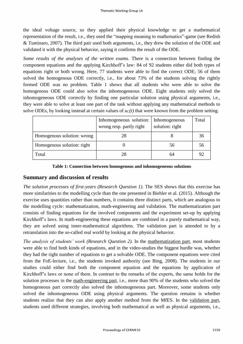
Some results of the analyses of the written exams. There is a connection between finding the

component equations and the applying Kirchhoff’s law: 84 of 92 students either did both types of

equations right or both wrong. Here, 77 students were able to find the correct ODE; 56 of them

solved the homogenous ODE correctly, i.e., for about 73% of the students solving the rightly

formed ODE was no problem. Table 1 shows that all students who were able to solve the

homogenous ODE could also solve the inhomogeneous ODE. Eight students only solved the

inhomogeneous ODE correctly by finding one particular solution using physical arguments, i.e.,

they were able to solve at least one part of the task without applying any mathematical methods to

solve ODEs, by looking instead at certain values of uC(t) that were known from the problem setting.

Inhomogeneous solution:

wrong resp. partly right

Inhomogeneous

solution: right

Total

Homogenous solution: wrong 28 8 36

Homogenous solution: right 0 56 56

Total 28 64 92

Table 1: Connection between homogenous and inhomogeneous solutions

Summary and discussion of results

The solution processes of first-years (Research Question 1). The SES shows that this exercise has

more similarities to the modelling cycle than the one presented in Biehler et al. (2015). Although the

exercise uses quantities rather than numbers, it contains three distinct parts, which are analogous to

the modelling cycle: mathematization, math-engineering and validation. The mathematization part

consists of finding equations for the involved components and the experiment set-up by applying

Kirchhoff’s laws. In math-engineering these equations are combined in a purely mathematical way,

they are solved using inner-mathematical algorithms. The validation part is attended to by a

retranslation into the so-called real world by looking at the physical behavior.

The analysis of students’ work (Research Question 2). In the mathematization part, most students

were able to find both kinds of equations, and in the video-studies the biggest hurdle was, whether

they had the right number of equations to get a solvable ODE. The component equations were cited

from the FoE-lecture, i.e., the students invoked authority (see Bing, 2008). The students in our

studies could either find both the component equation and the equations by application of

Kirchhoff’s laws or none of them. In contrast to the remarks of the experts, the same holds for the

solution processes in the math-engineering part, i.e., more than 90% of the students who solved the

homogeneous part correctly also solved the inhomogeneous part. Moreover, some students only

solved the inhomogeneous ODE using physical arguments. The question remains is whether

students realize that they can also apply another method from the MfES. In the validation part,

students used different strategies, involving both mathematical as well as physical arguments, i.e.,

some students did all steps of the modelling cycle, while others argued using inner-mathematical

arguments. They showed different justification strategies, analogous to justifications like calculation

and physical mapping, as defined in Bing, 2008.

Acknowledgments

Project was funded by the German Federal Ministry of Education and Research (BMBF) under

contract FKZ 01PK11021B.

References

Alpers, B. (2015). Differences between the usage of mathematical concepts in engineering statics

and engineering mathematics education. In R. Göller, R. Biehler, R. Hochmuth & H. G. Rück

(Eds.), Didactics of Mathematics in Higher Education as a Scientific Discipline (pp. 138–142),

khdm-Report 16-05. Kassel: Universitätsbibliothek Kassel. Retrieved from http://nbn-

resolving.de/urn:nbn:de:hebis:34-2016041950121

Biehler, R., Kortemeyer, J., & Schaper, N. (2015). Conceptualizing and studying students' processes

of solving typical problems in introductory engineering courses requiring mathematical

competences. In K. Krainer & N. Vondrová (Eds.), Proceedings of the Ninth Conference of the

European Society for Research in Mathematics Education (CERME9, 4-8 February 2015) (pp.

2060–2066). Prague, Czech Republic: Charles University in Prague, Faculty of Education and

ERME. Retrieved from https://hal.archives-ouvertes.fr/CERME9/public/CERME9_NEW.pdf

Bing, T. J. (2008). An epistemic framing analysis of upper level physics students’ use of

mathematics. Ph.D. thesis, University of Maryland. Retrieved from

http://drum.lib.umd.edu/bitstream/1903/8528/1/umi-umd-5594.pdf

Blum, W., & Leiss, D. (2007). How do students and teachers deal with modelling problems? In C.

Haines, P. Galbraith, W. Blum & S. Khan (Eds.), Mathematical modelling: Education,

engineering, and economics (pp. 222–231). Chichester: Horwood.

Hall, E. P., Gott, S. P., & Pokorny, R. A. (1995). A procedural guide to cognitive task analysis: The

PARI Methodology (No. AL/HR-TR-1995-0108). Armstrong Lab Brooks AFB TX Human

Resources Directorate. Retrieved from http://www.dtic.mil/dtic/tr/fulltext/u2/a303654.pdf

Polya, G. (1949). How to solve it: A new aspect of mathematical method. Princeton, New Jersey:

Princeton University Press.

Redish, E. F., (2005). Problem solving and the use of math in physics courses. In Proceedings of the

Conference, World View on Physics Education in 2005: Focusing on Change, Delhi, August 21-

26, 2005. Retrieved from http://www.physics.umd.edu/perg/papers/redish/IndiaMath.pdf

Tuminaro, J., & Redish E. F. (2007): Elements of a cognitive model of physics problem solving:

Epistemic games. Physical Review Special Topics - Physics Education Research 3 (020201), 1–

21. doi: http://dx.doi.org/10.1103/PhysRevSTPER.3.020101