The Interaction of Radio-Frequency Fields With Dielectric … · 2012-02-13 · actions with solid...

1. Introduction1.1 Background

In this paper we will overview electromagnetic inter-actions with solid and liquid dielectric and magneticmaterials from the macroscale down to the nanoscale.We will concentrate our effort on radio-frequency (RF)waves that include microwaves (MW) and millimeter-waves (MMW), as shown in Table 1. Radio frequencywaves encompass frequencies from 3 kHz to 300 GHz.Microwaves encompass frequencies from 300 MHz to30 GHz. Extremely high-frequency waves (EHF) andmillimeter waves range from 30 GHz to 300 GHz.

Many devices operate through the interaction of RFelectromagnetic waves with materials. The characteri-zation of the interface and interaction between fields

Volume 117 (2012) http://dx.doi.org/10.6028/jres.117.001Journal of Research of the National Institute of Standards and Technology

1

The Interaction of Radio-Frequency FieldsWith Dielectric Materials at

Macroscopic to Mesoscopic Scales

James Baker-Jarvis andSung Kim

Electromagnetics Division,National Institute of Standardsand Technology,Boulder, Colorado 80305

[email protected]@boulder.nist.gov

The goal of this paper is to overviewradio-frequency (RF) electromagneticinteractions with solid and liquid materialsfrom the macroscale to the nanoscale. Theoverview is geared toward the generalresearcher. Because this area of research isvast, this paper concentrates on currentlyactive research areas in the megahertz(MHz) through gigahertz (GHz)frequencies, and concentrates on dielectricresponse. The paper studies interactionmechanisms both from phenomenologicaland fundamental viewpoints. Relaxation,resonance, interface phenomena,plasmons, the concepts of permittivityand permeability, and relaxation times aresummarized. Topics of current researchinterest, such as negative-index behavior,noise, plasmonic behavior, RF heating,nanoscale materials, wave cloaking,polaritonic surface waves, biomaterials,and other topics are overviewed.

Relaxation, resonance, and relatedrelaxation times are overviewed. Thewavelength and material length scalesrequired to define permittivity in materialsis discussed.

Key words: dielectric; electromagneticfields; loss factor; metamaterials;microwave; millimeter wave; nanoscale;permeability; permittivity; plasmon;polariton.

Accepted: August 25, 2011

Published: February 2, 2012

http://dx.doi.org/10.6028/jres.117.001

Table 1. Radio-Frequency Bands [1]

frequency wavelength band

3 – 30 kHz 100 – 10 km VLF30 – 300 kHz 10 – 1 km LF0.3 – 3 MHz 1 – 0.1 km MF

3 – 30 MHz 100 – 10 m HF30 – 300 MHz 10 – 1 m VHF

300 – 3000 MHz 100 – 10 cm UHF3 – 30 GHz 10 – 1 cm SHF

30 – 300 GHz 10 – 1 mm EHF300 – 3000 GHz 1 – 0.1 mm THz


and materials is a critical task in any electromagnetic(EM) device or measurement instrument development,from nanoscale to larger scales. Electromagnetic wavesin the radio-frequency range have unique properties.These attributes include the ability to travel in guided-wave structures, the ability of antennas to launch wavesthat carry information over long distances, possessmeasurable phase and magnitude, the capability forimaging and memory storage, dielectric heating, andthe ability to penetrate materials.

Some of the applications we will study are related toareas in microelectronics, bioelectromagnetics, home-land security, nanoscale and macroscale probing,magnetic memories, dielectric nondestructive sensing,radiometry, dielectric heating, and microwave-assistedchemistry. For nanoscale devices the RF wavelengthsare much larger than the device. In many other applica-tions the feature size may be comparable or larger thanthe wavelength of the applied field.

We will begin with an introduction of the interactionof fields with materials and then overview the basicnotations and definitions of EM quantities, thenprogress into dielectric and magnetic response, defini-tions of permittivity and permeability, fields, relaxationtimes, surfaces waves, artificial materials, dielectric and magnetic heating, nanoscale interactions, and fieldfluctuations. The paper ends with an overview ofbiomaterials in EM fields and metrologic issues.Because this area is very broad, we limit our analysis toemphasize solid and liquid dielectrics over magneticmaterials, higher frequencies over low frequencies,and classical over quantum-mechanical descriptions.Limited space will be used to overview electrostaticfields, radiative fields, and terahertz interactions. Thereis minimal discussion of EM interactions with non-linear materials and gases.

1.2 Electromagnetic Interactions From theMicroscale to Macroscale

In this section we want to briefly discuss electromag-netic interaction with materials on the microscale to themacroscale.

Matter is modeled as being composed of manyuncharged and charged particles including for example,protons, electrons, and ions. On the other hand, theelectromagnetic field is composed of photons. Theinternal electric field in a material is related to the sumof the fields from all of the charged particles plusany applied field. When particles such as biological

molecules, cells, or inorganic materials are subjected toexternal electric fields, the molecules can respond in anumber of ways. For example, a single charged particlewill experience a force in an applied electric field. Also,in response to electric fields, the charges in a neutralmany-body particle may separate to form induceddipole moments, which tend to align in the field; how-ever this alignment is in competition with thermaleffects. Particles that have permanent dipole momentswill interact with applied dc or high-frequency fields.In an electric field, particles with permanent dipole-moments will tend to align due to the electrical torque,but in competition to thermal randomizing effects.When EM fields are applied to elongated particles withmobile charges, they tend to align in the field. If thefield is nonuniform, the particle may experience dielec-trophoresis forces due to field gradients.

On the microscopic level we know that the electro-magnetic field is modeled as a collection of photons[2]. In theory, the electromagnetic field interactionswith matter may be modeled on a microscopic scale bysolving Schrödinger’s equation, but generally otherapproximate approaches are used. At larger scales theinteraction with materials is modeled by macroscopicMaxwell’s equations together with constitutive rela-tions and boundary conditions. At a courser level ofdescription, phenomenological and circuit models arecommonly used. Typical scales of various objects areshown in Fig. 1. The mesoscopic scale is whereclassical analysis begins to be modified by quantummechanics and is a particularly difficult area to model.

The interaction of the radiation field with atomsis described by quantum electrodynamics. From aquantum-mechanical viewpoint the radiation field isquantized, with the energy of a photon of angularfrequency ω being E = ω. Photons exhibit wave-duality and quantization. This quantization also occursin mechanical behavior where lattice vibrationalmotion is quantized into phonons. Commonly, an atomis modeled as a harmonic oscillator that absorbs oremits photons. The field is also quantized, and eachfield mode is represented as a harmonic oscillator andthe photon is the quantum particle.

The radiation field is usually assumed to contain adistribution of various photon frequencies. When theradiation field interacts with atoms at the appropriatefrequency, there can be absorption or emission ofphotons. When an atom emits a photon, the energy ofthe atom decreases, but then the field energy increases.Rigorous studies of the interaction of the molecular


2 http://dx.doi.org/10.6028/jres.117.001

field with the radiation field involve quantization of theradiation field by expressing the potential energyV(r) and vector potential A(r, t) in terms of creation andannihilation operators and using these fields in theHamiltonian, which is then used in the Schrödingerequation to obtain the wavefunction (see, for example,[3]). The static electromagnetic field is sometimesmodeled by virtual photons that can exist for the shortperiods allowed by the uncertainty principle. Photonscan interact by depositing all their energy in photo-electric electron interactions, by Compton scatteringprocesses, where they deposit only a portion of theenergy together with a scattered photon, or by pairproduction. When a photon collides with an electron itdeposits its kinetic energy into the surrounding matteras it moves through the material. Light scattering is aresult of changes in the media caused by the incomingelectromagnetic waves [4]. In Rayleigh elastic lightscattering, the photons of the scattered incident lightare used for imaging material features. Brillouinscattering is an inelastic collision that may form orannihilate quasiparticles such as phonons, plasmons,and magnons. Plasmons relate to plasma oscillations,often in metals, that mimic a particle and magnons arethe quanta in spin waves. Brillouin scattering occurswhen the frequency of the scattered light shifts inrelation to the incident field. This energy shift relates

to the energy of the interacting quasiparticles. Brillouinscattering can be used to probe mesoscopic propertiessuch as elasticity. Raman scattering is an inelasticprocess similar to Brillouin scattering, but where thescattering is due to molecular or atomic-level transi-tions. Raman scattering can be used to probe chemicaland molecular structure. Surface-enhanced Ramanscattering (SERS) is due to enhancement of the EMfield by surface-wave excitation [5].

Optically transparent materials such as glass haveatoms with bound electrons whose absorption frequen-cies are not in the visible spectrum and, therefore, inci-dent light is transmitted through the material. Metallicmaterials contain free electrons that have a distributionof resonant frequencies that either absorb incominglight or reflect it. Materials that are absorbing in onefrequency band may be transparent in another band.

Polarization in atoms and molecules can be due topermanent electric moments or induced momentscaused by the applied field, and spins or spin moments.The response of induced polarization is usually weakerthan that of permanent polarization, because the typicalradii of atoms are on the order of 0.1 nm. On applica-tion of a strong external electric field, the electroncloud will displace the bound electrons only about10–16 m. This is a consequence of the fact that theatomic electric fields in the atom are very intense,


3

Fig. 1. Scales of objects.


approximately 1011 V/m. The splitting of spectral linesdue to the interaction of electric fields with atoms andmolecules is called the Stark effect. The Stark effectoccurs when interaction of the electric-dipole momentof molecules interacts with an applied electric field thatchanges the potential energy and promotes rotation andatomic transitions. Because the rotation of the mole-cules depends on the frequency of the applied field, theStark effect depends on both the frequency and fieldstrength. The interaction of magnetic fields with molec-ular dipole moments is called the Zeeman effect. Boththe Stark and Zeeman effects have fine-structure modi-fications that depend on the molecule’s angularmomentum and spin. On a mesoscopic scale, the inter-actions are summarized in the Hamiltonian that con-tains the internal energy of the lattice, electric and mag-netic dipole moments, and the applied fields.

In modeling EM interactions at macroscopic scales,a homogenization process is usually applied and theclassical Maxwell field is treated as an average of thephoton field. There also is a homogenization processthat is used in deriving the macroscopic Maxwellequations from the microscopic Maxwell equations.The macroscopic Maxwell’s equations in materials areformed by averaging the microscopic equations over aunit cell. In this averaging procedure, the macroscopiccharge and current densities, the magnetic field H, themagnetization M, the displacement field D, and theelectric polarization field P are formed. At these scales,the molecule dipole moments are averaged over a unitcell to form continuous dielectric and magnetic polar-izations P and M. The constitutive relations for thepolarization and magnetization are used to define thepermittivity and permeability. At macroscopic to meso-scopic scales the permittivity, permeability, refractiveindex, and impedance are used to model the response ofmaterials to applied fields. We will discuss this in detailin Sec. 4.5. Quantities such as permittivity, permeabili-ty, refractive index, and wave impedance are not micro-scopic quantities, but are defined through an averagingprocedure. This averaging works well when the wave-length is much larger than the size of the molecules oratoms and when there are a large number of molecules.In theoretical formulations for small scales and wave-lengths near molecular dimensions, the dipole momentand polarizability tensor of atoms and molecules can beused rather than the permittivity or permeability. In somematerials, such as magnetoelectric and chiral materials,there is a coupling between the electric and magneticresponses. In such cases the time-harmonic constitutive

relations are B~

(ω) = μH~

(ω) + η1 E~

(ω) and D~

(ω) =εE

~(ω) + η2 H

~(ω). In most materials the constitutive

relations B~

(ω) = μ 0 (M~

(ω) + H~

(ω)) and D~

(ω) =ε0 E

~(ω) + P

~(ω) are used.

In any complex lossy system, energy is convertedfrom one form to another, such as the transformation ofEM energy to lattice kinetic energy and thermal energythrough photon-phonon interactions. Some of theenergy in the applied fields that interact with materialsis transfered into thermal energy as infrared phonons.In a waveguide, there is a constant exchange of energybetween the charge in the guiding conductors and thefields [6].

When the electromagnetic field interacts with mate-rial degrees of freedom, a collective response may begenerated. The term polariton relates to bosonic quasi-particles resulting from the coupling of EM photons orwaves with an electric or magnetic dipole-carryingexcitation [4, 5]. The resonant and nonresonantcoupling of EM fields in phonon scattering is mediatedthrough the phonon-polariton transverse-wave quasi-particle. Phonon polaritons are formed from photonsinteracting with terahertz to optical phonons.Ensembles of electrons in metals form plasmas andhigh-frequency fields applied to these electron gasesproduce resonant quasi-particles, commonly calledplasmons. Plasmons are a collective excitation of agroup of electrons or ions that simultaneously oscillatein the field. An example of a plasmon is the resonantoscillation of free electrons in metals and semiconduc-tors in response to an applied high-frequency field.Plasmons may also form at the interface of a dielectricand a metal and travel as a surface wave with most ofthe EM energy confined to the low-loss dielectric. Asurface plasmon polariton is the coupling of a photonwith surface plasmons. Whereas transverse plasmonscan couple to an EM field directly, longitudinalplasmons couple to the EM field by secondary particlecollisions. In the microwave and millimeter wavebands artificial structures can be machined in metallicsurfaces to produce plasmons-like excitations due togeometry. Magnetic coupling is mediated throughmagnons and spin waves. A magnon is a quantum of aspin wave that travels through a spin lattice. A polaronis an excitation caused by a polarized electron travelingthrough a material together with the resultant polariza-tion of adjacent dipoles and lattice distortion [4]. All ofthese effects are manifest at the mesoscale throughmacroscale in the constitutive relations and the result-ant permittivity and permeability.



1.3 Responses to Applied RF Fields

If we immerse a specimen in an applied field and theresponse is recorded by a measurement device, the dataobtained are usually in terms of a digital readout or aneedle deflection indicating the phase and magnitude ofa voltage or current, a difference in voltage andcurrent, power, force, temperature, or an interferencefringe. For example, we deduce electric and magneticfield strengths and phase through Ampere’s andFaraday’s laws by means of voltage and currentmeasurements. The scattering parameters measured ona network analyzer relates to the phase and magnitudeof a voltage wave. The detection of a photon’s energy issensed by an electron cascade current. Cavities andmicrowave evanescent probes sense material character-istics through shifts in resonance frequency from theinfluence of the specimen under test. The shift in reso-nance frequency is again determined by voltage andpower measurements on a network analyzer. Magneticinteractions are also determined through measurementsof current and voltage or forces [4, 7-9]. These measure-ment results are usually used with theoretical models,such as Maxwell’s equations, circuit parameters, or theDrude model, to obtain material properties.

High-frequency electrical responses include the meas-urement of the phase and magnitude of guided waves intransmission lines, fields from antennas, resonant fre-quencies and quality factors (Q) of cavities or dielectricresonators, voltage waves, movement of charge or spin,temperature changes, or forces on charge or spins. Theseresponses are then combined through theoretical modelsto obtain approximations to important fundamentalquantities such as: power, impedance, capacitance,inductance, conductance, resistance, conductivity, resis-tivity, dipole and spin moments, permittivity, and perme-ability, resonance frequency, Q, antenna gain, and near-field response [10-16].

The homogenization procedure used to obtain themacroscopic Maxwell equations from the microscopicMaxwell equations is accomplished by averaging themolecular dipole moments within a unit cell and con-structing an averaged continuous charge density func-tion. Then a Taylor series expansion of the averagedcharge density is performed, and, as a consequence, itis possible to define the averaged polarization vector.The spatial requirement for the validity of this averag-ing is that the wavelength must be much larger than theunit cell dimensions (see Sec. 4.6 ). According to thisanalysis, the permittivity of an ensemble of moleculesis valid for applied field wavelengths that are muchlarger than the dimensions of an ensemble of molecules

or lattice, assuming one can isolate the effects of themolecules from the measurement apparatus. Thismetrology is not always easy because a measurementcontains effects of electrodes, probes, and otherenvironmental factors. The concepts of atomic polariz-ability and dipole molecular moment are valid on asmaller scale than are permittivity and permeability.

In the absence of an applied field, small randomvoltages with a zero mean are produced by equilibriumthermal fluctuations of random charge motion [17].Fluctuations of these random voltages create electricalnoise power in circuits. Analogously, spin noise is dueto spin fluctuations. Quasi-monochromatic surfacewaves can also be excited by random thermal fluctua-tions. These surface waves are different from black-body radiation [18]. Various interesting effects areachieved by random fields interacting with surfaces.For example, surface waves on two closely spacedsurfaces can cause an enhanced radiative transfer.Noise in nonequilibrium systems is becoming moreimportant in nanoscale measurements and in systemswhere the temperatures vary in time. The informationobtained from radiometry at a large scale, or micro-scopic probing of thermal fluctuations of variousmaterial quantities, can produce an abundance of infor-mation on the systems under test.

1.4 RF Measurements at Various Scales

At RF frequencies the wavelengths are much largerthan molecular dimensions. There are various approach-es to obtaining material response with long wavelengthfields to study small-scale particles or systems. Thesemethods may use very sensitive detectors, such assingle-charge or spin detectors or amplifiers, or averagethe response over an ensemble of particles to obtain acollective response. To make progress in the area ofmesoscale measurement, detector sensitivity may needto exceed the three or four significant digits obtainedfrom network analyzer scattering parameter measure-ments, or one must use large ensembles of cells for abulk response and infer the small-scale response.Increased sensitivity may be obtained by using resonantmethods or evanescent fields.

Material properties such as collective polarizationand loss [19] are commonly obtained by immersingmaterials in the fields of EM cavities, dielectricresonators, free-space methods, or transmission lines.Some responses relate to intrinsic resonances in amaterial, such as polariton or plasmon response,ferromagnetic and anti-ferromagnetic resonances, andterahertz molecular resonances.



Broadband response is usually obtained by use oftransmission lines or antenna-based systems [12-14,19, 20]. Thin films are commonly measured withcoplanar waveguides or microstrips [14]. Commonmethods used to measure material properties at smallscales include near-field probes, micro-transmissionlines, atomic-force microscopes, and lenses.

In strong fields, biological cells may rotate, deform,or be destroyed [21]. In addition, when there is morethan one particle in the applied field, the fields betweenthe particles can be modified by the presence ofnearby particles. In a study by Friend et al. [22], theresponse of an amoeba to an applied field was studiedin a capacitor at various voltages, power, and frequen-cies. They found that at 1 kHz and at 10 V/cm theamoeba oriented perpendicular to the field. At around10 kHz and above 15 V/cm the amoeba’s internalmembrane started to fail. Above 100 kHz and a fieldstrength of above 50 V/cm, thermal effects started todamage the cells.

1.5 Electromagnetic Measurement ProblemsUnique to Microscale and Nanoscale Systems

Usually, the electrical skin depth for field penetrationis much larger than the dimensions of nanoparticles.Because nanoscale systems are only 10 to 1000 timeslarger than the scale of atoms and small molecules,quantum mechanics plays a role in the transport prop-erties. Below about 10 nm, many of the continuousquantities in classical electromagnetics take on a quan-tized aspect. These include charge transport, capaci-tance, inductance, and conductance. Fluctuations involtage and current also become more important than inmacroscopic systems. Electrical conduction at the10 nanoscale involves movement of a small number ofcharge carriers through thin structures and may attainballistic transport. For example, if a 1 μA chargetravels through a nanowire of radial dimensions 30 nm,then the current density is on the order of 3 × 109 A/m2.Because of these large current densities, electricaltransport in nanoscale systems is usually a non-equilibrium process, and there is a large influence ofelectron-electron and electron-ion interactions.

In nanoscale systems, boundary layers and interfacesstrongly influence the electrical properties, and the localpermittivity may vary with position [23]. Measurementson these scales must model the contact resistancebetween the nanoparticle and the probe or transmissionline and deal with noise.

2. Fundamental ElectromagneticParameters and Concepts Used inMaterial Characterization

2.1 Electrical Parameters for High-FrequencyCharacterization

In this section, the basic concepts and tools needed tostudy and interpret dielectric and magnetic responseover RF frequencies are reviewed [24].

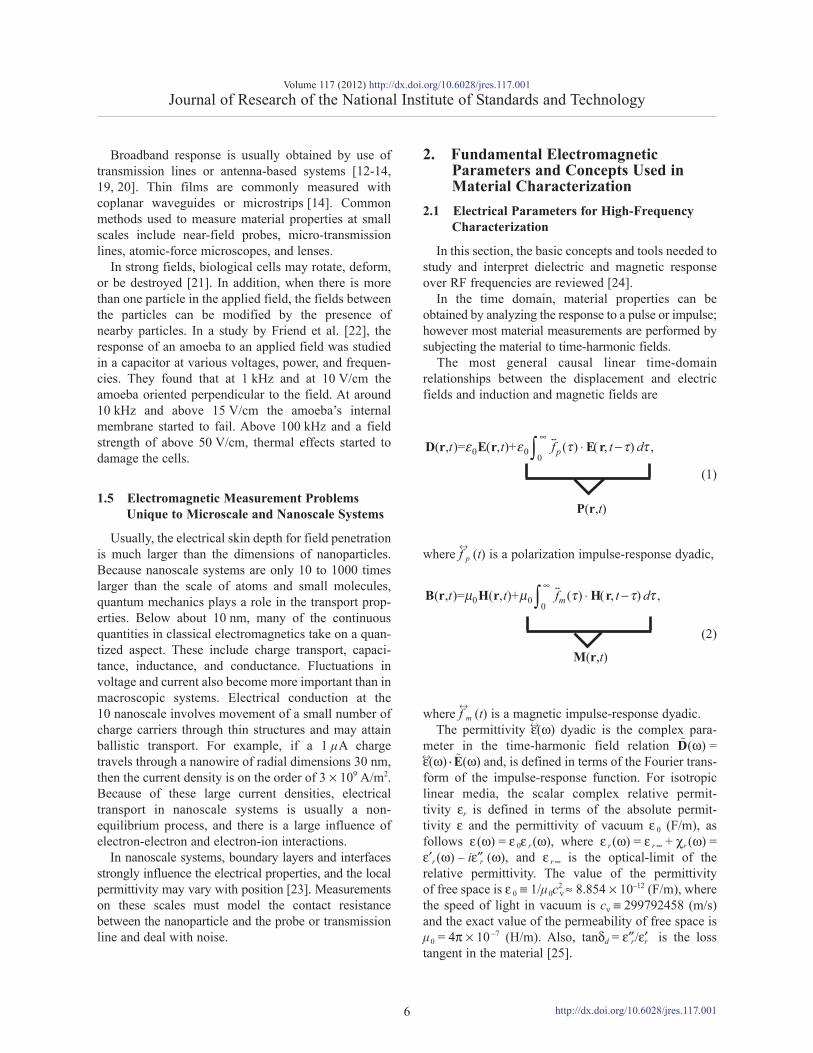
In the time domain, material properties can beobtained by analyzing the response to a pulse or impulse;however most material measurements are performed bysubjecting the material to time-harmonic fields.

The most general causal linear time-domainrelationships between the displacement and electricfields and induction and magnetic fields are

(1)

where f↔

p (t) is a polarization impulse-response dyadic,

(2)

where f↔

m (t) is a magnetic impulse-response dyadic.The permittivity ε↔(ω) dyadic is the complex para-

meter in the time-harmonic field relation D~

(ω) =ε↔(ω) .E

~(ω) and, is defined in terms of the Fourier trans-

form of the impulse-response function. For isotropiclinear media, the scalar complex relative permit-tivity εr is defined in terms of the absolute permit-tivity ε and the permittivity of vacuum ε 0 (F/m), asfollows ε (ω) = ε 0ε r(ω), where ε r(ω) = ε r ∞ + χr (ω) =ε′r(ω) – iε″r (ω), and ε r ∞ is the optical-limit of therelative permittivity. The value of the permittivityof free space is ε 0 ≡ 1/μ0c2

ν ≈ 8.854 × 10–12 (F/m), wherethe speed of light in vacuum is cν ≡ 299792458 (m/s)and the exact value of the permeability of free space isμ0 = 4π × 10 –7 (H/m). Also, tanδd = ε″r/ε′r is the losstangent in the material [25].


6

0 00

( , )= ( , )+ ( ) ( , ) ,ε ε τ τ τ∞

⋅ −∫

pt t f t dD r E r E r

0 00

( , )= ( , )+ ( ) ( , ) ,μ μ τ τ τ∞

⋅ −∫mt t f t dB r H r H r

P(r,t)

M(r,t)


Note that in the SI system of units the speed of light,permittivity of vacuum, and permeability of vacuumare defined constants. All measurements are related toa frequency standard. Note that the minus sign beforethe imaginary part of the permittivity and permeabilityis due to the e iωt time dependence. A subscript eff on thepermittivity or permeability releases the quantity fromsome of the strict details of electrodynamic analysis.The permeability in no applied field is: μ(ω) =μ0(μ′r (ω) – iμ″r (ω)) and the magnetic loss tangent istanδm = μ″r(ω)/μ′r (ω).

For anisotropic and gyrotropic media with an appliedmagnetic field, the permittivity and permeabilitytensors are hermitian and can be expressed in thegeneral form

(3)

For a definition of gyrotropic media see [4]. The off-diagonal elements are due to gyrotropic behavior in anapplied field.

Electric and magnetic fields are attenuated as theytravel through lossy materials. Using time-harmonicsignals the loss can be studied at specific frequencies,where the time dependence is e iωt. The change in losswith frequency is related to dispersion.

The propagation coefficient of a plane wave isγ = α + iβ = ik =coefficient in an infinitely thick half space, where theguided wavelength of the applied field is much longerthan the size of the molecules or inclusions, is denotedby the quantity α and the phase is denoted by β. Due tolosses of a plane wave, the wave amplitude decays as|E| ∝ exp(–αz). The power in a plane wave of the formE(z, t) = E0 exp (–αz) exp (iωt – iβz), attenuates asP ∝ exp (–2αz). For waves in a guided structure:

wavenumber, and speed of light c . Below cutoff, the

plane wave is given by

and has units of Np/m. α is approximated for dielectricmaterials as

(5)

In dielectric media with low loss, tanδd <<1, and α

reduces in this limit to α → ω

skin depth is the distance a plane wave travels until itdecays to 1/e of its initial amplitude, and is related tothe attenuation coefficient by δs = 1/α. The concept ofskin depth is useful in modeling lossy dielectrics andmetals. Energy conservation constrains a to be positive.The skin depth is defined for lossy dielectric materialsas

(6)

In Eq. (6), δs reduces in the low-conductivity limit to

to δs → 2c/(ωDp = δs /2 is the depth where the plane-wave energydrops to 1/e of its value on the surface. In metals, wherethe conductivity is large, the skin depth reduces to

(7)

where σdc is the dc conductivity and f is the frequency.We see that the frequency, conductivity, and perme-ability of the material determine the skin depth inmetals.

The phase coefficient β for a plane wave is given by

In dielectric media, β reduces to

(9)

The imaginary part of the propagation coefficientdefines the phase of an EM wave and is related to the

refractive index bythe positive square root is taken in Eq. (8). Veselago[26] developed a theory of negative-index materials(NIM) where he used negative intrinsic


7

( ) .xx xy z xz y

xy z yy yz x

xz y yz x zz

ig ig

ig ig

ig ig

ε ε ε

ε ε ε ε

ε ε ε

⎛ ⎞− +⎜ ⎟

ω = + −⎜ ⎟⎜ ⎟⎜ ⎟− +⎝ ⎠

. The plane-wave attenuationi εμω

2 2 , where / 2 / is the cutoffγ ω π λ= − = =c c c ci k k k c

2 2propagation coefficient becomes . of aγ α= −ck k

2 2 1/2

1/2

(((tan tan 1) (tan tan ) )2

(tan tan 1)) ,

ωα ε μ δ δ δ δ

δ δ

= − + +

+ −

r r d m d m

d m

' 'c

21 tan 1 .2

ωα ε μ δ= + −r r d' 'c

tan /2 . Theε μ δr r d' ' c

2

2 1 .1 tan 1

δε μ δ

=ω + −

s

r r d

c

' '

tan ). The depth of penetrationε μ δr r d' '

0

1δπ μ μ σ

=sr dcf '

21 tan 1 .2

ωβ ε μ δ= ± + +r r d' 'c

. In normaldielectricsε μ= ± r rn ' '

(4)

2 2 1/2

1/2

(((tan tan 1) (tan tan ) )2

(tan tan 1)) .

ωβ ε μ δ δ δ δ

δ δ

=± − + +

− −

r r d m d m

d m

' 'c

(8)


ε′r and μ′r , and the negative square root in Eq. (8) isused. There is controversy over the interpretation ofmetamaterial NIM electrical behavior since the perme-ability and permittivity are commonly effective values.We will use the term NIM to describe materials thatachieve negative effective permittivity and permeabili-ty over a band of frequencies.

The wave impedance for a transverse electricand magnetic mode (TEM) is

magnetic mode (TM) is γ / iωε. The propagating planewave wavelength in a material is decreased by a permit-tivity greater than that of vacuum; for example, for a

The surface impedance in ohms/square of a conduct-ing material is Zm = (1 + i )σδs . The surface resistancefor highly lossy materials is

(10)

When the conductors on a substrate are very thin, thefields can penetrate through the conductors into thesubstrate. This increases the resistance of a propagatingfield because it is in both the metal and the dielectric.As a consequence of the skin depth, the internal induc-tance in a highly-conducting material decreases withincreasing frequency, whereas the surface resistance Rs

increases with frequency in proportion to √f—.Any transmission line will have propagation delay

that relates to the propagation speed in the line. This isrelated to the dielectric permittivity and the geometryof the transmission line. Propagation loss is due toconductor and material loss.

Some materials exhibit ionic conductivity, so thatwhen a static electric field is applied, a current isinduced. This behavior is modeled by the dc conductiv-ity σdc , which produces a low-frequency loss (∝ 1/ω) inaddition to polarization loss (ε″r ). In some materials,such as semiconductors and disordered solids, theconductivity is complex and depends on frequency.This is because the free charge is partially bound andmoves by tunneling through potential wells or hopsfrom well to well.

The total permittivity for linear, isotropic materialsthat includes both dielectric loss and dc conductivity

is defined from the Fourier transform of Maxwell’sequation: iω D

~(ω) + J

~(ω) ≡ iωε E

~(ω) + σdc E

~(ω) ≡

iωεt o t E~

(ω), so that

(11)

In plots of RF measurements, the decibel scale isoften used to report power or voltage measurements.The decibel (dB) is a relative unit and for power iscalculated by 10 log10 (Pout /Pin). Voltages in decibelsare defined as 20 log10 (Vout / Vin). α has units ofNp/m. The attenuation can be converted from1 Np/m = 8.686 dB/m. dBm is similar to dB, but rela-tive to power in milliwatts 10 log(P/mW).

2.2 Electromagnetic Power

In the time domain the internal field energy U satis-fies: ∂U/∂t = ∂D/∂t · E + ∂B/∂t · H. Using Maxwell’sequations with a current density J, then producesPoynting’s Theorem: ∂U/∂t + ∇ · (E × H) = – J · E,where the time-domain Poynting vector is S(r, t) =E(r, t) × H(r, t). The complex power flux (W/m2)is summarized by the complex Poynting vector Sc(ω) ==(1/2)(E

~(ω) × H

~ * (ω)). The real part of Sc representsdissipation and is the time average over a completecycle. The imaginary part of Sc relates to the reactivestored energy.

2.3 Quality Factor

The band width of a resonance is usually modeled bythe quality factor (Q) in terms of the decay of theinternal energy. The combined internal energy in amechanical system is the kinetic plus the potentialenergy; in an electromagnetic system it is the fieldstored energy plus the potential energy. In the timedomain the quality factor is related to the decay of theinternal energy for an unforced resonator as as [27]

(12)

The EM field is modeled by a damped harmonicoscillator at frequencies around the lossless resonantfrequency ω0 and frequency pulling factor (the resonantfrequency decreases from ω0 due to material losses),Δω as [27]

(13)


8

/ ; for a transverseμ εelectric mode (TE) is / , and for a transversei μ γω

TEM mode, /( ). In waveguides theguid-λ ε μ≈ vac r rc ' ' fed wavelength dependson the cutoff wavelengthg cλ λ

2 2 2 2and is given by 1/ / 1/ / 1 ( / ) .g c c' 'f cλ ε μ λ λ λ λ= − = −

01 .π μ μ

δ σ σ= = r

ss dc dc

f 'R

o 0 0( ) .σε ε ε ε εω

= − + dct t i' ''

r r

0

0

( ) ( ) .ω

= −dU t U tdt Q

0 0/ 2 ( )0( ) .ω 0− ω +Δω= t Q i tE t E e e


Taking a Fourier transform of Eq. (13), the absolutevalue squared becomes

(14)

and therefore |E(ω)|2, which is proportional to thepower, is a Lorentzian. This linear model is not exactfor dispersive materials, because Q0 may be dependenton frequency. The quality factor is calculated from thefrequency at resonance f0 as Q0 = f0 / 2(| f 0 – f 3dB|), orfrom a fit of a circle when plotting S11(ω) on the Smithchart. The quality factor is calculated from Q0 = f 0/Δf ,where Δf is the frequency difference between 3 dBpoints on the S21 curve [28]. For resonant cavity meas-urements, the permittivity or permeability is deter-mined from measurements of the resonance frequencyand quality factor, as shown in Fig. 2. For time-harmonic fields the Q is related to the stored fieldenergies We ,Wh , the angular frequency at resonance ωr ,and the power dissipated Pd at the resonant frequency:

(15)

Resonant frequencies can be measured with highprecision in high-Q systems; however the parasiticcoupling of the fields to fixtures or materials needs tobe modeled in order to make the result meaningful.Material measurements using resonances have muchhigher precision than using nonresonant transmissionlines.

The term antiresonance is used when the reactivepart of the impedance of a EM system is very high. Thisis in contrast to resonance, where the reactance goes tozero. In a circuit consisting of a capacitor and induc-tance in parallel, antiresonance occurs when the voltageand current are in phase.

3. Maxwell’s Equations in Materials3.1 Maxwell’s Equations From Microscopic to

Macroscopic Scales

Maxwell’s microscopic equations in a media withcharged particles are written in terms of the micro-scopic fields b, e and sources j, and ρm as

(16)

(17)

(18)

(19)

Note, that at this level of description the macroscopicmagnetic field H and the macroscopic displacementfield D are not defined, but can be formed by averagingdielectric and magnetic moments and expanding themicroscopic charge density in a Taylor series. Inperforming the averaging process, the material lengthscales allow the dipole moments in the media to beapproximated by continuously varying functions P andM. Once the averaging is completed, the macroscopicMaxwell’s equations are (see Sec. 4.6) to obtain[27, 29, 30]

(20)

(21)

(22)

(23)

J denotes the current density due to free charge andsource currents. Because there are more unknowns thanequations, constitutive relations for H and D are need-ed. Even though B and E are the most fundamentalfields, D usually is expressed in terms of E, and B isusually expressed in terms of H.


9

2

2 2

0

( ) ,( ) ( )

20

ω =ωω − ω − Δω +

AE

Q

.e hr

d

W WQ

P+

= ω

Fig. 2. Measuring resonant frequency and Q.

0 0 0 ,t

ε μ μ∂∇× = +∂eb j

,∂∇× = −∂tbe

0 ,mε ∇ ⋅ = ρe

0.∇ ⋅ =b

,t

∂∇× = +∂DH J

,∂∇× = −∂tBE

,∇ ⋅ = ρD

.∇ ⋅ = 0B


3.2 Constitutive Relations3.2.1 Linear Constitutive Relations

Since there are more unknowns than macroscopicMaxwell’s equations, we must specify the constitutiverelationships between the polarization, magnetization,and current density as functions of the macroscopicelectric and magnetic fields [31, 32]. In order to satisfythe requirements of linear superposition, any linearpolarization relation must be time invariant, further,this must also be a causal relationship as given inEqs. (1) and (2).

The fields and material-related quantities inMaxwell’s equations must satisfy underlying sym-metries. For example, the dielectric polarization andelectric fields are odd under parity transformations andeven under time-reversal transformations. The magne-tization and induction fields are even under paritytransformation and odd under time reversal. Thesesymmetry relationships place constraints on the natureof the allowed constitutive relationships and requiresthe constitutive relations to manifest related sym-metries [29, 33-39]. The evolution equations for theconstitutive relationships need to be causal, and inlinear approximations must satisfy time-invarianceproperties. For example, the linear-superpositionrequirement is not satisfied if the relaxation time inEq. (4) depends on time. This can be remedied by usingan integrodifferential equation with restoring anddriving terms [40, 41].

The macroscopic displacement and induction fieldsD and B are related to the macroscopic electric field Eand magnetic fields H, as well as M and P, by

(24)and

(25)

In addition,

(26)

where J is a function of the electric and magneticfields, and Q

↔is the macroscopic quadrupole moment

density. Pd is the dipolemoment density, whereas P isthe effective macroscopic polarization that alsoincludes the effects of the macroscopic quadrupole-moment density [27, 29, 30, 32, 42]. The polarizationand magnetization for time-domain linear response areexpressed as convolutions in terms of the macroscopic

fields. For chiral and magneto-electric materials, Eqs.(24) and (25) must be modified to accommodate cross-coupling behavior between magnetic and dielectricresponse. General, linear relations defining polarizationin non-magnetoelectric and non-chiral dielectric andmagnetic materials in terms of the impulse-responsedyadics are given by Eqs. (1) and (2). Using theLaplace transform L, gives

(27)

where

(28)

So the real part is the even function of frequency given by

(29)

and the imaginary part is an odd function of frequency

(30)

and therefore

(31)

also(32)

(33)

The time-evolution constitutive relations for dielec-tric materials are generally summarized by generalizedharmonic oscillator equations or Debye-like equationsas overviewed in Sec. 5.2.

3.2.2 Generalized Constitutive RelationsThrough the methods of nonequilibrium quantum-

based statistical-mechanics it is possible to show thatthe constitutive relation for the magnetization in ferro-magnetic materials is an evolution equation given by

(34)

where K↔

m is a kernel that contains of the micro-structural interactions given in [43], γg is the gyro-magnetic ratio, χ0 is the static susceptibility, and Heff


10

0 0 ,dε ε= + − ∇ ⋅ + ≡ +D E P Q E P

0 0 .μ μ= +B H M

( , ) ,= JJ E H

( ) ( ) ( ) ,L χω = ω ω erÑ E

0( ) ( ) ( ) ( ).i t

er p er erf e dt ' i ''χ τ χ χ∞ − ωω = = ω − ω∫

0( ) ( )cos( ) ,er p' f t t dtχ

∞ω = ω∫

0( ) ( )sin( ) ,er p" f t t dtχ

∞ω = ω∫

( ) ( ) ( );r er erI ' i ''ε χ χω = + ω − ω

0( ) ( ) ,

( ) 0 .

er p

er

f t dtχ

χ

∞′ 0 =

′′ 0 =

∫

30

0

( , ) ( , ) ( , )

( , , , ) ( , ) ,

g eff

tm eff

t t tt

d r t d

γ

τ χ τ τ

∂ = − ×∂

′ ′ ′− ⋅∫ ∫

M r M r H r

K r r H r


is the effective magnetic field. Special cases of Eq. (34)reduce to constitutive relations such as the Landau-Lifshitz, Gilbert, and Bloch equations. The Landau-Lifshitz equation of motion is useful for ferromagneticand ferrite solid materials:

(35)

where α is a damping constant. Another special case ofEq. (34) reduces to the Gilbert equation

(36)

In electron-spin resonance (EPR) and nuclearmagnetic resonance (NMR) measurements, the Blochequations with characteristic relaxation times T1 and T2

are used to model relaxation. T1 relates to spin-latticerelaxation as the paramagnetic material interacts withthe lattice. T2 relates to spin-spin interactions:

(37)

where χ↔b has only the diagonal elements χb (11) = 1/T2 ,χb (22) = 1/T2 , χb (33) = 1/T1 , and Ms = Msz

→. An equationanalogous to (34) can be written for the electricalpolarization [46] as [43]

(38)

The Debye relaxation differential equation isrecovered from Eq. (38) when K

↔e (r, t , r′, τ) =

I↔

δ(t – τ)δ(r, – r′)/τe .

4. Electromagnetic Fields in Materials4.1 The Time-Harmonic Field Approximation

Time-harmonic fields are very useful for solving thelinear Maxwell’s equations when transients are notimportant. In the time harmonic field approximation,the field is assumed to be present without beginning orend. Periodic signals over − ∞ < t < ∞ are nonphysi-cal since all fields have a beginning where transientsare generated, but are very useful in probing materialresponse.

Solutions of Maxwell’s equations that includetransients are most easily obtained with the Laplacetransform. Note that the Laplace or Fourier transformedfields do not have the same units as the time-harmonicfields due to integration over time. In Eq. (1), causalityis incorporated into the convolution relation for linearresponse. D(t) depends only on E(t) at earlier times andnot future times.

4.2 Material Response to Applied Fields

When a field is suddenly applied to a material, thecharges, spins, currents, and dipoles in a mediumrespond to the local fields to form an average field. Ifan EM field is suddenly applied to a semi-infinitematerial, the total field will include the effects of boththe applied field, transients, and the particle back-reaction fields from charge, spin, and current rearrange-ment that causes depolarization fields. This will causethe system to be in nonequilibrium for a period of time.For example, as shown in Fig. 3, when an applied EMfield interacts with a dielectric material, the dipolesreorient and charge moves, so that the macroscopic andlocal fields in the material are modified by surfacecharge dipole depolarization fields that oppose theapplied field. The macroscopic field is approximatelythe applied field minus the depolarization field.Depolarization, demagnetization, thermal expansion,exchange, nonequilibrium, and anisotropy interactionscan influence the dipole orientations and therefore thefields and the internal energy. In modeling the constitu-tive relations in Maxwell’s equations, we must expressthe material properties in terms of the macroscopicfield, not the applied or local fields, and therefore weneed to make clear distinctions between the interactionprocesses [40].

Materials can be studied by the response of frequen-cy-domain or time-domain fields. When consideringtime-domain pulses rather than time-harmonic fields,


11

( , ) ( , )( , )precession

( , ) ( ( , ) ( , ))M

,damping

γ

α γ

×∂ ≈ −∂

− × ×

g eff

geff

t ttt

t t ts

M r H rM r

M r M r H r

∨∨

s

( , ) ( , ) ( , )

( , )( , ) .M

γ

α

∂ ≈ − ×∂

∂+ ×∂

g efft t t

ttt

t

M r M r H r

M rM r

1

( , ) ( , ) ( , )

( , ) ,

g

sb

t t tt

tT

γ

χ

∂ ≈ − ×∂

− ⋅ +

M r M r H r

MM r

( )

3

0

0

( , ) ( , , , )

( , ) ( , ) .

te

t d r tt

d

τ

τ χ τ τ

∂ ′ ′= −∂

′ ′× − ⋅

∫ ∫P r K r r

P r E r

∨∨


this interaction is more complex. The use of time-domain pulses have the advantage of sampling areflected pulse as a function of time, which allows adetermination of the spatial location of the variousreflections.

Time-harmonic fields are often used to study materi-al properties. These have a specific frequency fromtime minus infinity to plus infinity, without transients;that is, fields with a e iωt time dependence. As a conse-quence, in the frequency domain, materials can bestudied through the reaction to periodic signals. Themeasured response relates to how the dipoles andcharge respond to the time-harmonic signal at eachfrequency. If the frequency information is broadenough, a Fourier transform can be used to study thecorresponding time-domain signal.

The relationships between the applied, macroscopic,local, and the microscopic fields are important forconstitutive modeling (Fig. 3). The applied fieldoriginates from external charges, whereas the macro-scopic fields are averaged quantities in the medium.The displacement and inductive (or magnetic) macro-scopic fields in Maxwell’s equations are implicitlydefined through the constitutive relationships andboundary conditions. The local field is the averagedEM field at a particle site due to both the applied fieldand the fields from all of the other sources, such asdipoles, currents, charge, and spin [47]. The micro-scopic field represents the atomic-level EM field,where particles interact with the field from discretecharges. Particles interact with the local EM field thatis formed from the applied field and the microscopicfield. At the next level of homogenization, groupsof particles interact with the macroscopic field. Thespatial and temporal resolution contained in the macro-

scopic variables are directly related to the spatial andtemporal detail incorporated in the constitutive material parameters. Constitutive relations can be exact as in[40] and Eqs. (34) and (38), but usually, to be useful,are approximate.

Plane waves are a useful approximation in manyapplications. Time-harmonic EM plane waves in mate-rials can be treated either as traveling without attenua-tion, propagating with attenuation, or evanescent. Planewaves may propagate in the form of a propa-gating wave e i(ωt – βz), or a damped propagating wavee i(ωt – βz) – αz, or an evanescent wave e iωt – αz. Evanescentfields are exponentially damped waves. In a wave-guide, this occurs for frequencies below any transverseresonance frequencies [24, 48], when k2 – k2

c < 0, wherekc is the cutoff wave number calculated from the

Evanescent and near field EM fields occur at aperturesand in the vicinity of antennas. Evanescent fields can bedetected when they are perturbed and converted intopropagating waves or transformed by dielectric loss.Electromagnetic waves may convert from near field topropagating. For example, in coupling to dielectricresonators the near field at the coupling loops producepropagating or standing waves in a cavity or dielectricresonator. Evanescent and near fields in dielectricmeasurements are very important. These fields do notpropagate and are used in near-field microwave probesto measure or image materials at dimensions much lessthan λ/2 [49, 50] (see Fig. 17). The term near field usu-ally refers to the waves close to an waveguide, antenna,or probe and is not necessarily an exponentiallydamped plane wave. In near-field problems the goal isto model the reactive region. Near fields in the reactiveregion, (L < λ/2π), contain stored energy and there isno net energy transport over a cycle unless there arelosses in the medium. By analogy, the far field relatesto radiation. These remove energy from the transmitterwhether they are immediately absorbed or not. There isa transition region called the radiative near field.

Because electrical measurements can now be per-formed at very small spatial resolutions, and theelements of electrical circuits are approaching themolecular level, we require good models of the macro-scopic and local fields. This is particularly important,because we know that the Lorentz theory of the localfield is not always adequate for predicting polarizabili-ties [51, 52]. Also, when solving Maxwell’s equationsat the molecular level, definitions of the macroscopic


12

Fig. 3. Fields in materials.

transverse geometry and ( / ) .ω εμ ω ε μ= = r rk c ' '


field and constituative relationships are important. Atheoretical analysis of the local EM field is importantin dielectric modeling of single-molecule measure-ments and thin films. The effective EM fields at thislevel are local, but not atomic-scale, fields.

The formation of the local field is a very complexprocess whereby the applied electric field polarizesdipoles in a molecules or lattices and the appliedmagnetic field causes current and precession of spins.Then, the molecule’s dipole field modifies the dipoleorientations of other molecules in close proximity,which then reacts back to produce a correction to themolecule’s field in the given region. This process getsmore complicated for behavior that depends on time.We define the local EM field as the effective, averagedfield at a specific point in a material, not including thefield of the particle itself. This field is a function ofboth the applied and multipole fields in the media. Thelocal field is related to the average macroscopic andmicroscopic EM fields in that it is a sum of the macro-scopic field and the effects of the near-field. In ferro-electric materials, the local electric field can becomevery large and hence there is a need for comprehensivelocal field models. In the literature on dielectric materi-als, a number of specific fields have been introduced toanalyze polarization phenomena. The electric fieldacting on a nonpolar dielectric is commonly called theinternal field, whereas the field acting on a permanentdipole moment is called the directing field. The differ-ence between the internal field and directing fields isthe average reaction field. The reaction field is theresult of a dipole polarizing its environment [53].

Nearly exact classical theories have been developedfor the static local field. Mandel and Mazur developeda static theory for the local field in terms of the polar-ization response of a many-body system by use ofthe T-matrix formalism [54]. Gubernatis extended theT-matrix formalism [55]. However, the T-matrix contri-butions are difficult to calculate. Keller’s review article[56] on the local field uses an EM propagator approach.Kubo’s linear-response theory and other theories havealso been used for EM correlation studies [40, 53, 57].

If the applied field has a wavelength that is not muchlonger than the typical particle size in a material, aneffective permittivity and permeability is commonlyassigned. The terms effective permittivity and perme-ability are commonly used in the literature for studiesof composite media. The assumption is that the proper-ties are “effective” if in some sense they do not adhereto the definitions of the intrinsic material properties. Aneffective permittivity is obtained by taking a ratio ofsome averaged displacement field to an averaged

electric field. The effective permeability is obtained bytaking a ratio of some averaged induction field to anaveraged magnetic field. This approach is commonlyused in modeling negative-index material propertieswhen scatterers are designed in such a manner such thatthe scatterers themselves resonate. In these situationsthe wavelength may approach the dimensions of theinclusions.

4.3 Macroscopic and Local Electromagnetic Fieldsin Materials

The mesoscopic description of the EM fields in amaterial is complicated. As a field is applied to amaterial, charges reorient to form new fields thatoppose the applied field. In addition, a dipole tends topolarize its immediate environment, which modifiesthe field the dipole experiences. The field that polarizesa molecule is the local field El and the induced dipolemoment is p = α↔. El , where α↔ is the polarizability. Inorder to use this expression in Maxwell’s equations, thelocal field needs to be expressed in terms of the macro-scopic field. Calculation of this relationship is notalways simple.

To first approximation, the macroscopic field isrelated to the external or applied field (Ea), and thedepolarization field by

(39)

The local field is composed of the macroscopic fieldand a material-related field. In the literature, the effec-tive local field is commonly modeled by the Lorentzfield, which is defined as the field in a small cavity thatis carved out of a material around a specific site, butexcludes the field of the observation dipole. A well-known example of the relationship between theapplied, macroscopic, and local fields is given by ananalysis of the Lorentz spherical cavity in a staticelectric field. For a Lorentz sphere the local field is thesum of applied, depolarization, Lorentz, and atomicfields [4, 56, 58]:

(40)

For cubic lattices in a spherical cavity, the Lorentz localfield is related to the macroscopic field and polarizationby

(41)


13

1 .3 0

= −εaE E P

= + + + .t a depol Lorentz atomE E E E E

1 .3 0

= +εlE E P


In the case of a sphere, the local field in Eq. (39) equalsthe applied field.

For induced dipoles,

(42)

where N is the density of dipoles, and Eq. (41) yieldsEl = E/(1 – Nα/3ε0 ) = P/Nα.

Onsager [53] generalized the Lorentz theory bydistinguishing between the internal field that acts oninduced dipoles and the directing field that acts onpermanent dipoles. If we use P = ε0 (εr – 1)E inEq. (41), we find El = ((εr + 2)/3)E. Therefore, fornormal materials the Lorentz field exceeds the macro-scopic field. For a material where the permittivity isnegative we can have El ≤ E. In principle, we can nullout the Lorentz field when εr = – 2. Some of the essen-tial problems encountered in microscopic constitutivetheory center around the local field. Note that for somematerials, recent research indicates that the Lorentzlocal field does not always lead to the correct polariz-abilities [51]. We expect the Lorentz local field expres-sion to break down near interfaces. For nanoparticles, amore complicated theory needs to be used for the localfield.

A rigorous expression for the static local field creat-ed by a group of induced dipoles can be obtained by aniterative procedure [53, 59] using pi = αiEl(ri) and

(43)

where

(44)

If there are also permanent dipoles, they need to beincluded as p(ri) = pperm(ri) + αiEl (ri ).

4.4 Overview of Linear-Response Theory

Models of relaxation that are based on statisticalmechanics can be developed from linear-responsetheory. Linear-response theory uses an approximatesolution of Liouville’s equation and a Hamiltonian thatcontains a time-dependent relationship of the fieldparameters based on a perturbation expansion. Thisapproach shows how the response functions and

relaxation are related to time dependent polarizationcorrelation functions. The polarization P(t) is related tothe response dyadic φ↔ (t) and the driving field E(t) by[53, 60]

(45)

where φ↔ (t – τ) = 0 for t – τ < 0. The susceptibility isdefined as

(46)

where the response in volume V is related to the corre-lation function for stationary processes in terms of themicroscopic polarization

(47)

and therefore for microscopic polarizations

(48)

Once the correlation functions are determined thenthe susceptibility can be found. An approach thatmodels relaxation beyond linear response is given in[40, 43, 44, 61]. The method of linear response hasexceeded expectations and has been a cornerstone ofstatistical mechanics.

4.5 Averaging to Obtain Macroscopic Field

If we consider modeling of EM wave propagationfrom macroscopic through molecular and sub-molecu-lar to atomic scales, the effective response at each levelis related to different degrees of homogenization. Atwavelengths short relative to particle size the EM prop-agation is dominated by scattering, whereas at longwavelengths it is dominated by traveling waves. Inmicroelectrodynamics, there have been many types ofensemble and volumetric averaging methods used to


14

,lNα=P E

,

( ) ( ) ,n

i j a ij ji l i j= ≠

= + ∑E r E E r

5 30

3( ) ( ) ( )1( ) , .4

⎡ ⎤−⎢ ⎥≈ −⎢ ⎥πε − −⎢ ⎥⎣ ⎦

j i i iij j

j i j i

r r p r p rE r

r r r r

( ) ( ) ( )t

t t d−∞

= φ − τ ⋅ τ τ,∫P E

( ) τ∞ − ω

0χ(ω) = φ τ τ = χ (ω)− χ (ω) ,∫

i ' ''e d i

(0)τ

0< (τ) >φ(τ) = − ,

B

dVd k T

p p

0

0

00

00

(0)

(0) ( ) sin( )

(0) ( ) cos( ) .

ωτ

ωτ

∞ −

∞ − 0

∞

∞

χ(ω) = φ(τ) τ =

< (τ) >− τ

τω ⎡= < τ > ωτ τ−⎢⎣

⎤< τ > ωτ τ⎥⎦

∫∫

∫

∫

i

i

B

B

e d

dV e dd k T

V dk T

i d

p p

p p

p p


define the macroscopic fields obtained from the micro-scopic fields [27, 29, 30, 40, 54]. For example, in themost commonly used theory of microelectromagnetics,materials are averaged at a molecular level to produceeffective molecular dipole moments. The microscopicEM theories developed by Jackson, Mazur, andRobinson [27, 29, 30] average multipoles at a molecu-lar level and replace the molecular multipoles, withaveraged point multipoles usually located at the center-of-mass position. This approach works well down tonear molecular level, but breaks down below themolecular to submolecular level.

In the various approaches, the homogenization of thefields are formed in different ways. The averaging isalways volumetric rather than a time average. Jacksonuses a truncated averaging test function to proceedfrom microscale to the macroscale fields [27]. Robinsonand Mazur use ensemble averaging [29, 30] and statis-tical mechanics. Ensemble averaging assumes there is adistribution of states. In the volumetric averagingapproach, the averaging function is not explicitly deter-mined, but the function is assumed to be such that theaveraged quantities vary in a manner smooth enough toallow a Taylor-series expansion to be performed. In theapproach of Mazur, Robinson, and Jackson [27, 29, 30]the charge density is expanded in a Taylor series andthe multipole moments are identified as in Eq. (49).The microscopic charge density can be related to themacroscopic charge density, polarization, and quadru-pole density by a Taylor-series expansion [27]

(49)where Q

↔(r, t) is the quadrupole tensor. In this inter-

pretation, the concepts of P and ρmacro are valid at lengthscales where a Taylor-series expansion is valid. Thesemoments are calculated about each molecular center ofmass and are treated as point multipoles. However, thistype of molecular averaging limits the scales of thetheory to larger than the molecular level and limits themodeling of induced-dipole molecular moments [40].Usually, the averaging approach uses a test function fa

and microscopic field e given by

(50)

However, the distribution function is seldom explic-itly needed or determined in the analysis. The macro-scopic magnetic polarization is found through an anal-ogous expansion of the microscopic current density.

In NIM materials, effective properties are obtainedby use of electric and magnetic resonances of embed-ded structures that produce negative effective ε′ef f [62].In Sec. 4.6 the issue of whether this response can besummarized in terms of material parameters is dis-cussed. Defining permittivity and permeability on thesescales of periodic media can be confusing. The fieldaveraging used in NIM analysis is based on a unit cellconsisting of split-ring resonators, wires, and ferrite ordielectric spheres [62, 63].

In order to obtain a negative effective permeability inNIM applications, researchers have used circuits thatare resonant, which can be achieved by the introductionof a capacitance into an inductive system. Pendry et al.[63-65] obtained the required capacitance through gapsin split-ring resonators. The details of the calculation ofeffective permeability are discussed in Reference [63].Many passive and/or active microwave resonantdevices can be used as sources of effective perme-ability in the periodic structure designed for NIMapplications [66]. We should note that the compositematerials used in NIM are usually anisotropic. Also, theuse of resonances in NIM applications produce effec-tive material parameters that are spatially varying andfrequency dispersive.

4.6 Averaging to Obtain Permittivity andPermeability in Materials

The goal of this section is to study the electricalpermittivity and permeability in materials starting frommicroscopic concepts and then progressing to macro-scopic concepts. We will study the limitations of theconcept of permittivity in describing material behaviorwhen wavelengths of the applied field approach thedimensions of the spaces between inclusions orinclusion sizes. When high-frequency fields are used inthe measurement of composite and artificial structures,these length-scale constraints are important. We willalso examine alternative quantities, such as dipolemoment and polarizability, that characterize dielectricand magnetic interactions of molecules, atoms, and thatare still valid even when the concepts of permittivityand permeability are fuzzy.

The concepts of polarizability and dipole momentp in p = αEl are valid down to the atomic and molecu-lar levels. Permittivity and permeability are frequency-domain concepts that result from the microscopic time-harmonic form of Maxwell’s equations averaged over aunit cell. They are also related to the Fourier transformof the impulse-response function. The most common


15

( , ) ( , ) ( , ) ( Q)( , ),< ρ >≈ ρ −∇⋅ −∇ ⋅ ∇ ⋅

micro macror t r t r t r tP

( ) ( ) .ad ' ' f '= −∫E r e r r r


way to define ε↔ is through the impulse-response func-tion f

↔p (t).

Statistical mechanics yields an expression for theimpulse-response function in terms of correlation func-tions of the microscopic polarizations p. For linearresponse [53]

(51)

where V is the volume, L0 is Liouville’s operator,p. denotes iL0p, and < >0 denotes averaging over phase.From this equation, we can identify the impulse-response dyadic f

↔p from P(t) = V ∫∞0< p (t)p. (τ) >0 · E(τ)

dτ / kBT , and for a stationary system, f↔

p(t) =V < p (0)p. (– t) >0 /kBT [53].

Ensemble and volumetric averaging methods areused to obtain the macroscopic fields from the micro-scopic fields (see Jackson [27] and the referencestherein). For example, in the most commonly usedtheory, materials are averaged at a molecular level toproduce effective molecular dipole moments. Whenderiving the macroscopic Maxwell’s equations fromthe microscopic equations, the electric and magneticmultipoles within a molecule are replaced with aver-aged point multipoles usually located at the molecularcenter-of-mass positions. Then these effective momentsare assumed to form a continuum, which then forms thebasis of the macroscopic polarizations. The procedureassumes that the wavelength in the material is muchlarger than the individual particle sizes. As Jackson[27] notes, the macroscopic Maxwell’s equations canmodel refraction and reflection of visible light, but arenot as useful for modeling x-ray diffraction. He statesthat the length scale L0 of 10 nanometers is effectivelythe lower limit for the validity of the macroscopicequations. Of course, this limit can be decreased withimproved constitutive relationships.

For macroscopic heterogeneous materials the wave-lengths of the applied fields must be much longerthan individual particle or molecule dimensions thatconstitute the material. When this criterion does nothold, then the spatial derivative in the macroscopicMaxwell’s equations, for example, (∇ × H), and thedisplacement field loses its meaning. Associated withthis homogenization process at a given frequency is thenumber of molecules or inclusions that are required todefine a displacement field and thereby the relatedpermittivity.

When the ratio of the dipole length scale to wave-length is not very small, the Taylor’s series expansionis not valid and the homogenization procedure breaksdown. When this criteria is not satisfied for metafilms,some researchers use generalized sheet transition con-ditions (GSTC’s) [67-70] at the material boundaries;however, the concept of permittivity for these struc-tures, at these frequencies, is still in question and iscommonly assigned an effective value. Drude andothers [67, 68] compensated for this by introducingboundary layers. In such cases, it is not clear whethermapping complicated field behavior onto effectivepermittivity and permeability is useful, since at thesescales, the results can just as well be thought of asscattering behavior.

When modeling the permittivity or permeability in amacroscopic medium in a cavity or transmission line,the artifacts of the measurement fixture must beseparated from the material properties by solving arelevant macroscopic boundary-value problem. Atmicrowave and millimeter frequencies a low-lossmacroscopic material can be made to resonate as adielectric resonator. In such cases, if the appropriateboundary-value problem is solved, the intrinsic permit-tivity and permeability of the material can be extractedbecause the wavelengths are larger than the constituentmolecule sizes, and as a result, the polarization vectoris well defined. However, many modern applicationsare based on artificial structures that produce an EMresponse where the wavelength in the material is onlyslightly larger than the feature or inclusion size. In suchcases, mapping the EM response onto a permittivityand permeability must be scrutinized. In general, thepermittivity is well defined in materials where wavepropagation through the material is not dominated bymultiple scattering events.

5. Overview of the Dielectric Response toApplied Fields

5.1 Modeling Dielectric Response UponApplication of an External Field

Dielectric parameters play a critical role in manytechnological areas. These areas include electronics,microelectronics, remote sensing, radiometry, dielectricheating, and EM-assisted chemistry [20]. At RFfrequencies dielectrics exhibit behavior that metalscannot achieve because dielectrics allow field penetra-tion and can have low-to-medium loss characteristics.


16

0 ( )0

0( )

t i tp

B

d V e ddt k T

−τ= < > ⋅ τ τ ,∫P p p E L


Using dielectric spectroscopy as functions of bothfrequency and temperature we can obtain some, but notall of the information on a material’s molecular orlattice structure. For example, measurements of thepolarization and conductivity indicate the polarizabilityand free charge of a material and polymer mobility ofside chains can be studied with dielectric spectroscopy.Also, when a polymer approaches a glass transitiontemperature the relaxation times change abruptly.This is observable with dielectric spectroscopy. Inaddition, the loss peaks of many liquids change withtemperature.

When an EM field is applied to a material, the atoms,molecules, free charge, and defects adjust positions. Ifthe applied field is static, then the system will eventu-ally reach an equilibrium state. However, if the appliedfield is time dependent then the material will continu-ously relax in the applied field, but with a time lag. Thetime lag is due to screening, coupling, friction, andinertia. An abundance of processes are occurring duringrelaxation, such as heat conversion processes, lattice-phonon, and photon phonon coupling. Dielectric relax-ation can be a result of dipolar and induced polariza-tion, lattice-phonon interactions, defect diffusion,higher multipole interactions, or the motion of freecharges. Time-dependent fields produce nonequilibri-um behavior in the materials due both to the heatgenerated in the process and the constant response tothe applied field. However, for linear materials andtime-harmonic fields, when the response is averagedover a cycle, if heating is appreciable, nonequilibriumeffects such as entropy production relate more totemperature effects than the driving field stimulus. Thedynamic readjustment of the molecules in responseto the field is called relaxation and is distinct fromresonance. For example, if a dc electric field is appliedto a polarizable dielectric and then the field is sudden-ly turned off, then the dipoles will relax over a charac-teristic relaxation time into a more random state.

The response of materials depends strongly onmaterial composition and lattice structure. In manysolids, such as solid polyethylene, the molecules are notable to appreciably rotate or polarize in response toapplied fields, indicating a low permittivity and smalldispersion. The degree of crystallinity, existence ofpermanent dipoles, dipole-constraining forces, mobilityof free charge, and defects all contribute to dielectricresponse. Typical responses for high-loss and low-lossdielectrics are shown in Figs. 4, 5, and 6.


17

Fig. 4. Broadband permittivity variation for materials [71].

Fig. 5. Typical frequency dependence of ε′r of low-loss fused silicaas measured by many methods.

Fig. 6. Typical frequency dependence of the loss tangent in low-lossmaterials such as fused silica.


A material does not respond instantaneously to anapplied field. As shown in Fig. 4, the real part of thepermittivity is a monotonically decreasing function offrequency in the relaxation part of the spectrum, faraway from intrinsic resonances. At low frequencies, thedipoles generally follow the field, but thermal agitationalso tends to randomize the dipoles. As the frequencyincreases to the MMW band, the response to the driv-ing field generally becomes more incoherent. At higherfrequencies, in the terahertz or infrared spectrum, thedipoles may resonate, and therefore the permittivityrises until it becomes out of phase with the field andthen drops. At RF frequencies, materials with low lossrespond differently from materials with high loss(compare Fig. 4 for a high-loss material versus a low-loss material in Figs. 5 and 6). For some materials, atfrequencies at the low to middle part of the THz band,ε′r may start to contain some of the effects of resonancesthat occur at higher frequencies, and may start toslowly increase with frequency, until resonance, andthen decreases again.

The local and applied fields in a dielectric areusually not the same. As the applied field interacts witha material it is modified by the fields of the moleculesin the substance. Due to screening, the local electricfield differs from the applied field and thereforetheories of relaxation must model the local field (seeSec. 4.3).

Over the years, many models of polar and nonpolar-materials have been developed that use differentapproximations to the local field. The Clausius-Mossotti equation was developed for noninteracting,nonpolar molecules governed by the Lorentz equationfor the internal field. This equation works well for non-polar gases and liquids. Debye introduced a generaliza-tion of the Clausius-Mossotti equation for the case ofpolar molecules. Onsager developed an extension ofDebye’s theory by including the reaction field and amore comprehensive local field expression [53]. For adielectric composed of permanent dipoles, the polariza-tion is written in terms of the local field as Eq. (42)

There are electronic, ionic, and permanent dipolepolarizability contributions, so that μ→d = (αel + αion +αperm )El , αel = 4πε0R3 / 3, αion = e2 / Yd0 . Here, Y isYoung’s modulus, R is the radius of the ions, d0 isthe equilibrium separation of the ions, and αperm =|μ→e |2 /3kBT, where μ→e is the permanent dipole moment.There may also be a contribution to the polarizabilitydue to excess charge at microscopic interfaces. Using

the Lorentz expression for the local field, the polariza-tion can be written as

(52)

or

(53)

This is the Clausius-Mossotti relation that is common-ly used to estimate the permittivity of nonpolarmaterials from atomic polarizabilities:

(54)

or

(55)

The Clausius-Mossotti relation relates the permittivityto the polarizability. The polarizability is related to thevector dipole moment μ→d of a molecule or atom andthe local field El , μ→d = αEl . In principle, once thepolarizability is determined for a group of molecules,then the permittivity of the ensemble can be calculatedwith the implicit assumption that there are many mole-cules located over the distance of a wavelength. Typicalpolarizabilities of atoms are between 0.1 and 100 Fm2

[72]. Polarizabilities of molecules can be higher thanfor atoms. The local field for a sphere is related to thepolarization by Eq. (41).

A generalization of the Clausius-Mossotti equationto include a permanent moment μ→e is summarized inwhat is called the Debye equation that is valid for gasesand dilute solutions:

(56)

The Debye equation could be used to estimate thepermittivity of a gas if both the polarizability and thedipole moment were known from experiment.


18

0,

3Nα

ε⎛ ⎞

= +⎜ ⎟⎝ ⎠

PP E

( )00

1 .1 / 3 r

NNα ε εα ε

= = −−

EP E

0

1,

2 3r

r

Nαε −=

ε + ε

0

0

3 2.

3rN

Nαα

ε +ε =

ε −

2

0

1.

2 3 3er

r B

Nk Tμ

α⎛ ⎞ε − ⎜ ⎟= +⎜ ⎟ε + ε ⎝ ⎠


For a specific dipole immersed in an environment ofsurrounding dipoles, the dipole will tend to polarize thesurrounding dipoles and thereby create a reaction field.Onsager included the effects of the reaction field intothe local field and obtained the following relationshipfor the static field that, and unlike the Debye equation,can be used to model the dipole moment of some pureliquids:

(57)

where ε∞ is the optical limit of the permittivity. TheOnsager equation is often used to calculate dipolemoments of gases. Both atoms and molecules canpolarize when immersed in a field. Note that Eq. (57)uses the permittivity of the liquid, which is a macro-scopic quantity to estimate the microscopic dipolemoment.

5.2 Dielectric Relaxation and Resonance

5.2.1 Simple Differential Equations for Relaxationand Resonance

A very general, but simplistic equation, for modelingpolarization response that depends on time is given bya harmonic-oscillator relation:

(58)

where P is polarization, τ is the relaxation time, ω0

Various special cases of Eq. (58) serve as simple, naivemodels of relaxation, resonance, and plasmonicresponse. The first term relates to the effects of inertia,the second to dissipation, the third to restoring forces,and the RHS represents the driving forces. A weaknessof Eq.(58) is that the simple harmonic oscillator modelassumes only a single relaxation time, and resonancefrequency. This equation can be generalized to includeinteractions, (see Eq. (117)). In most materials, themolecules are coupled and have a broad range of relax-ation frequencies that widens the dielectric response.For time-harmonic fields Eq. (58) is

(59)

A resonance example is shown in Fig. 7. Intrinsicmaterial resonances in ionic solids can occur at highfrequencies due to driving at phonon normal-modefrequencies and relate to the mass inertial aspect in

sublattices.

If we eliminate the inertial interaction whenω2

0>> ω2, we have the time-domain Debye differentialequation for pure relaxation:

(60)

For time-harmonic fields, the Debye response is

(61)

Except for liquids like water, dielectrics rarely exhibitthe response of Eq. (61) since there is no singlerelaxation time over RF frequencies.

We generally assume that dipoles reorient in anapplied field in discrete jumps as the molecule makestransitions from one potential well minimum toanother with the accompanied movement of a polaronor defect in the lattice. The Debye model of relaxationassumes that dipoles relax individually with no inter-action between dipoles and with no inertia, but includesfrictional forces. The real part of the permittivity fordipolar systems generally does not exhibit single-poleDebye response, but rather a power-law dependence. The origin of this difference can be attributed to many-body effects that tend to smear the response over afrequency band.


19

22

) ),

)s s

es

kNΒΤμ 0 ∞ ∞

∞ 0

9 ε (ε − ε (2ε − ε=

ε (ε + 2ε

2

021 ,d d

dtdtχ2

0

+ τ + =ω

P P P E

0is the natural frequency ( / ), and .sk m0 ∞ω = χ = ε − ε

02( ) ( ).

1 i20

χω = ω

ω− + ωτω

P E

0 / of the positive and negative charges ofk mω =

Fig. 7. Theoretical resonance in the real part of the permittivity fromEq. (59) and associated loss factor.

0 .χτ + =ddtP P E

0( ) ( ).1 i

χω = ω

+ ωτP E


If we eliminate the restoring force term in Eq. (59),we have an equation of motion for charged plasmas,

(62)

For time-harmonic fields, this becomes

(63)

5.2.2 Modeling Relaxation in Dielectrics

The polarization of a material in an applied fielddepends on the permanent and induced dipolemoments, the local field, and their ability to rotate withthe field. Dielectric loss in polar materials is dueprimarily to the friction caused by rotation, free chargemovement, and out-of-phase dipole coupling. Losses innonpolar materials originate mainly from the inter-action with neighboring permanent and induceddipoles, intrinsic photon-phonon interactions with theEM field, and extrinsic loss mechanisms caused bydefects, dislocations, and grain structure. Loss in manyhigh-purity crystals is primarily intrinsic in that acrystal will vibrate nearly harmonically; however,anharmonic coupling to the electric field and thepresence of defects modifies this behavior. The an-harmonic interaction allows photon-phonon interactionand thereby introduces loss [73]. High-purity centro-symmetric dielectric crystals, that is, crystals withreflection symmetry, such as crystalline sapphire,strontium titanate, or quartz, have generally been foundto have lower loss than crystals with noncentro-symmetry [74].

A transient current may be induced if an electric fieldis applied, removed, or heated. This can be related tothe dielectric response. The depolarization current formany lossy disordered solids is nonexponential and, attime scales short relative to the relaxation time of themedia, can satisfy a power law of the form [75, 76]

(64)

and satisfy a power law at long times of the form

(65)

where 0 < n, m < 1. In this model, a short time scalecorresponds to frequencies in the microwave region(τ ∝ 1/ f < 1 × 10–9 s) and long relaxation times refer tofrequencies less than 10 kHz (τ ∝ 1/ f < 1 × 10–4 s). Inorder to satisfy theoretical constraints at very shortperiods the current must depart from Eq. (64). Thereare exceptions to the behavior given in Eqs. (64) and(65) in dipolar glasses, polycrystalline materials, andother materials [77]. The susceptibility of many lossydisordered solids typically behave at high frequenciesas a power law

(66)

This implies χ″ /χ′ is independent of frequency. On theother hand, measurements of many ceramics, glasses,and polymers exhibit a loss tangent that increasesapproximately linearly with frequency as shown inFig. 6.

Dissado and Hill conclude that nonexponentialrelaxation is related to cluster response [75]. In theirmodel, molecules within a correlated region react to theapplied field with a time delay. The crux of thisapproach is that in most condensed-matter systems therelaxation is due not to independently relaxing dipoles,but rather that the relaxation of a single dipole dependson the state of other dipoles in a cluster. Therefore theirmodel includes dipole-dipole coupling. This theory ofdisordered solids is based on charge hopping anddipolar transitions within regions surrounding a defectand between clusters [75]. The effect is to spread outthe response over time and therefore to produce non-exponential behavior. Dissado and Hill developed arepresentation of a correlation function that includescluster interaction. According to this theory, thetime-domain response for short time scales is Gaussiane– t 2 / τ 2 .

At longer periods there are intra-cluster transitionsthat follow a power law of the form t –n. At still longerperiods there are inter-cluster transitions with a Debye-type response e– t / τ, and finally at very long periodsthere is response of the form t – m – 1 [75].

Jonscher, Dissado, and Hill have developed theoriesof relaxation based on fractal self-similarity [78, 79].Jonscher’s approach is based on a screened-hoppingmodel where response is modified due to many-bodycharge screening [80]. In the limit of weak screening,the Debye model is recovered.

Nonexponential response has been obtained withmany models. In any materials where the dipoles do notrotate independently, the relaxation is nonexponential.


20

2

021 .d d

dtdtχ2

0

+ τ =ω

P P E

0( ) ( ).i

2

20

χω = ω

ω− + ωτω

P E

( ) ,nI t t−∝

(1 )( ) ,mI t t− +∝

( )1( ) ( ) .nχ χ −′ ′′ω ∝ ω ∝ ω


Nonexponential response has also been reproduced incomputer simulations for chains of dipoles by means ofa correlation-function approach with coupled rateEqs. [81-83].

Note that nonexponential time-domain response isactually required for over some bands in order to have acausal-function response over all frequencies. This is aconsequence of the Paley-Wiener theorem [84].According to this theorem, the correlation or decay func-tion cannot be a purely damped exponential func-tion for large times. If C(t) is the decay function then

(67)

must be finite. This requires the decay function tovanish less fast than a pure exponential at large times,C(t) ≈ exp (– ct q) where q < 1 and c is a constant. Wecan show that at short times, decay occurs faster thanexponential [85].

Nigmatullian et al. [86, 87] used the Mori-Zwanzigformalism to express the permittivity in a very generalform:

(68)

and concluded that for most disordered materials, theresponse is similar to that of a distributed circuit withR±(iω) = [(iωτ1)± ν 1+ (iωτ2)± ν 2]±, where νi are constantsdetermined by numerical fits. In the formulation ofBaker-Jarvis et al. [88], R± corresponds to the complexrelaxation times τ(ω) as R+(iω) = iωτ(ω) (see Sec. 11).A (iωτ)(n–1) frequency dependence of the complexrelaxation periods corresponds to a impulse-responsefunction of the form t – n.

In addition, in analyzing dielectric data the electricmodulus approach is sometimes used where M(ω) =M′ (ω)+iM″ (ω) = 1/εr = ε′r / (εr′2+ εr″2)+iεr″/ (εr′2+ εr″2).

Dielectric relaxation has also been described byKubo’s linear-response theory that is based on cor-relation functions. This is an example of a relaxationtheory derived from Liouville’s equation. The maindifficulty with these approaches is that the correlationfunctions are difficult to approximate to highlight theessential physics, and gross approximations are usuallymade in numerical calculations. The linear expansionof the probability-density function in Kubo’s theoryalso limits its usefulness for highly nonequilibriumproblems. Baker-Jarvis et al. have recently used astatistical-mechanical projection-operator methoddeveloped by Zwanzig and Robertson [89] to model

dielectric and magnetic relaxation response and theassociated entropy production [19, 40, 41, 43, 44].

6. The Distribution of Relaxation Times(DRT) Model for HomogeneousMaterials

There are many models used to fit measured frequen-cy-dependent dielectric relaxation data for homoge-neous materials. These models are usually generalenough to fit many types of response. When dealingwith heterogeneous materials, mixture equations arecommonly used (Sec. 22). The DRT model is restrictedto relaxation, and it assumes there is a probabilitydistribution y (t) that underpins the relaxation responsewith a relaxation time τ. In this model, the permittivitycan be written as

(69)

where

(70)

Note that DRT is a single-pole model and cannot beused for resonances. We see that in the DRT, Debyerelaxations are weighted by a probability-densityfunction. Equation (69) can be inverted by the Laplacetransform as shown in the Appendix of Böttcher [53].

The DRT approach is sufficiently general that mostcausal, relaxation dielectric-response phenomena canbe described by the model for Debye and power-lawresponse. In the DRT the slope of ε′r (ω) is alwaysnegative [90]. This is consistent with causality. It alsoindicates that the model is only valid for relaxation andnot resonance. Around resonance ε′r (ω) can increasewith frequency and become negative as indicated inFig. 7.

Equation (69) can fit the relaxation response ofmany dielectrics because the Debye equation originatesfrom a rate equation based on thermodynamics contain-ing the essential physics, and Eq. (69) is a distributionof Debye relaxations. The DRT then extends this into amulti-relaxation period rate equation. We considervarious special cases of Eq. (69) below. For otherspecial cases please see Böttcher [53]. In any complexdielectric material, we would expect there would be abroadening of relaxation times due to heterogeneity ofthe molecular response, and in this context the DRTmodel makes sense. This approach is often criticized,


21

log (,

1C

d∞

2−∞

τ) ||τ

+ τ∫

( ) ,1 ( )

∞∞

±

ε − εε ω = ε +

+ ωsiR i

0

( )( ) ( ) ,1 ( )

∞∞ ∞

τε ω = ε + ε − ε τ+ ωτ∫sy d

i

0( ) 1.y d

∞τ τ =∫


because it is not always possible obtain a physical inter-pretation of the distribution function [75].

6.1 Debye Model

The simplest case of the distribution function inEq. (69) is an uncorrelated approximation where

(71)

which yields the Debye response

(72)

In this case, the pulse response function is

(73)

In terms of components,

(74)

and

(75)

If ωτ is eliminated in the Debye model, and theequations for εr′(ω) and εr″ (ω) are plotted against eachother, we obtain the equation for a circle:

(76)

The center of the circle is on the horizontal axis.The reasons why the Debye equation is a paradigm

in dielectric relaxation theory is because it is simpleand contains the essential physics and thermodynamicsin relaxation. That is, it models idealized relaxation,and it yields predictions on the temperature dependenceof the relaxation time τ = A exp (Ea /RT), where Ea isthe activation energy.

6.2 Cole-Cole Model

The Cole-Cole model has been found useful formodeling many liquids, semisolids, and other materials[53]. In this case,

(77)

and

(78)

where α < 1. The pulse response function is fp (t) =

real and imaginary parts of the permittivity can beseparated into

(79)

(80)A plot of εr′(ω) versus εr″(ω) yields a circle, where thecenter is below the vertical axis.

6.3 Cole-Davidson Model

The Cole-Davidson model has also been founduseful for modeling many liquids, semisolids, and othermaterials [53]. If we consider the case τ ≤ τ0 :

(81)

and zero otherwise. The permittivity is

(82)

where β < 1. The pulse response function is

(83)

The real and imaginary parts of the permittivity can beseparated into

(84)

(85)

The plot of εr′(ω) versus εr″(ω) maps out a skewed arcrather than a circle.


22

( ) ( ) ,y t t= δ − τ

).

1∞

∞(ε − ε

ε = ε ++ ωτs

i

( ) exp( / ) / .pf t t= − τ τ

2( ) ,1

' sr

∞∞ 2

ε − εε ω = ε +

+ω τ

2 2

.2 2

s s2∞ ∞ε − ε ε − ε⎡ ⎤ ⎡ ⎤′ ′′ε (ω) − + ε (ω) =⎢ ⎥ ⎢ ⎥⎣ ⎦ ⎣ ⎦

2)

( ) .1

'' sr

∞2

(ε − ε ωτε ω =

+ω τ

1 sin( )2 cosh[(1 In cos

y0

πατ =π −α) τ/τ − πα]

10

,1 ( )

∞∞ −α

ε − εε(ω) = ε +

+ ωτs

i

(1 )0 00

(1/ ) ( 1) / (( 1)(1 ))( / ) . Them mm

m t∞ −α −α

=τ − Γ + −α τ∑

1

11 ( ) sin( )

( ) ( ) ,1 ( 2( ) sin( )

'r s

−α0

∞ ∞ 2(1−α) −α0 0

+ ωτ πα/2ε ω =ε + ε −ε

+ ωτ ) + ωτ πα/2

1

1( ) cos( )

( ) ( ) .1 ( 2( ) sin( )

''r s

−α0

∞ 2(1−α) −α0 0

ωτ πα/2ε ω = ε −ε

+ ωτ ) + ωτ πα/2

1( sinyβ

0

⎡ ⎤ττ) = πβ⎢ ⎥π τ − τ⎣ ⎦

)( ) ,

(1 )∞

∞ β0

(ε − εε ω = ε +

+ ωτs

r i

10 0 0( ) (1/ ( ))( / ) exp( / ) .β−= τ Γ β τ − τpf t t t

( ) ( )(1 ) cos ( [1 ]),2 2 −β/2∞ ∞ 0 0ε ω =ε + ε −ε +ω τ β + ωτ'

r s Arg i

( ) ( )(1 ) sin ( [1 ]) .2 2 −β/2∞ 0 0ε ω = ε −ε +ω τ β + ωτ''

r s Arg i


6.4 Havrilak-Negami Model

The Havrilak-Negami distribution has two para-meters to fit data and is very general. It can be used tofit the response of many liquids and non-Debye solidmaterials [53]. In the special case α = 0 it reverts to theCole-Davidson model. The distribution function is

(86)and θ = tan–1{sin π (1 – α) / (τ /τ0 + cos π (1 – α))}

(87)

where 0 < α ≤ 1 and 0 < β ≤ 1, and

(88)

(89)

7. Loss and Conductivity

Loss originates from the conversion of EM fieldenergy into heat and radiation through photon-phononinteractions. In dielectrics the heating is caused by thetransformation of electromagnetic energy into latticekinetic energy, which is seen as frictional forces ondipoles and the motion and resulting friction of freecharges in materials. Major mechanisms of conductionin dielectrics in the RF band are ionic or electrolyticmigration of free ions, impurities or vacancies, electro-phoretic migration of charged molecules, and elec-tronic conduction of semi-free electrons that originatefrom jump processes of polarons. At low frequencies,dipoles can respond to the changes in the applied field,so dielectric losses usually are low and the stored

energy is high, but as the frequency increases, thedipole response tends to fall behind the applied fieldand, therefore, the loss usually increases and the storedenergy decreases. This is related to the phasing betweenthe current and voltage waves, in analogy to the heatingan electric motor encounters when the phase betweenthe voltage and current changes.

Ionic conduction in insulating dielectrics is due tothe migration of charged ions. The migration takesplace through tunneling or jumps induced by theapplied field, or by slow migration under the appliedfield. In solid polymers it may proceed by jumps fromone vacancy to another or by electronic conduction. Inoxide glasses it is the movement of positively chargedalkali ions in the applied field. In many materials, thedielectric losses originate in vacancy-vacancy andvacancy-impurity relaxations.

At high frequencies, lossy semiconductors, super-conductors, and metals have a complex free-charge acconductivity that is explained by the Drude model. Thiscan cause the effective permittivity to become negative[27]. To understand this, consider Maxwell’s equation,

(90)

We can define an effective charge current as

(91)

or for time-harmonic fields

(92)

Combining ac J with the displacement field producesan effective real part of the permittivity that can benegative over a region of frequencies. For example inplasmas and superconductors, the effective conduct-ivity satisfies iωD∼ (ω) + J∼ (ω) = [iω(ε′(ω) – iε′′(ω)) +σ′(ω) – iσ′′(ω)]E∼ (ω), yielding

(93)

where σ′ ≈ σdc and σ″ relates to the reactive part of thesurface impedance. A large σ″ can produce a negativereal part of the total permittivity such as what occurs insuperconductors [91].


23

2

( ) sin1( ) ,

[( )] 2( ) cos(y

β(1−α)

0

(1−α) (1−α) β/2

0 0

τ βθτ

τ =τ τπ + π(1−α)) +1]τ τ

)( ) ,

(1 ( )∞

∞ 1−α β0

(ε − εε ω = ε +

+ ωτ )s

r i

2(1 / 2

( ) ( )cos ,1[1 2( sin ( ) ( ) )]2

∞ ∞

(1−α) −α) β0 0

ε ω = ε + ε − εβθ×

+ ωτ ) πα + ωτ

'r s

2(1 / 2

( ) ( )sin .1[1 2( sin ( ) ( ) )]2

∞ ∞

(1−α) −α) β0 0

ε ω = ε + ε − εβθ×

+ ωτ ) πα + ωτ

''r s

.∂ + = ∇×∂tD J H

( ) ( ) ( )t

e f f t t dt−∞

∂= σ − τ τ τ + ,∂∫ DJ E

( ) ( ( ) ( ) .e f f iω = σ ω) ω + ω ωJ E D

( )( ) ( )( ) ( ) ( ) ,e f f r r ri0 0

⎛ ⎞′′ ′σ ω σ ω′ ′′ε ω =ε ω − − ε ω +⎜ ⎟ε ω ε ω⎝ ⎠


A total conductivity has been used in the literature tomodel either the ac effects of the free charge andpartially bound free charge in hopping and tunnelingconduction, or as another way of re-expressing thecomplex permittivity. Because some charge is onlypartially bound, the distinction between conductivityand permittivity can, at times, get blurred. This blurringpoints out the mesoscopic property of the permittivity.Most models of ac conductivity are based on chargedparticles in potential wells where energy fluctuationsdetermine whether the particle can surmount a potentialbarrier and thereby contribute to the conductivity. Inconducting liquids, human tissue, and water-basedsemisolids the conductivity is generally flat withincreasing frequency until megahertz frequencies, andthen it increases, often in a nearly linear fashion.

There are a number of distinct models for σtot . TheDrude model of the complex conductivity of electronsor ions in a metal is approximately modeled as

(94)

where γ0 is the collision frequency, N is the electrondensity, m is the ion mass, and e is the electronic charge[27]. Note that the dc conductivity is σdc = Ne2 /mγ0 .The net dielectric response is a sum of the dipolarcontribution and that due to the ions, whereε′e f f = ε′d – Ne2 /m (γ2

0+ ω2) and ε″(ω) = Ne2γ0 /mω (γ20

+ ω2) + ε″d(ω). Therefore, for metals, the real part of thepermittivity is negative for frequencies near the plasma

metals is usually well above 100 GHz. The conduct-ivity is thermally active and can be modeled for someionic materials as [92]

(95)

where nc is the ion vacancy, b is the ion jump distance,ν0 is a characteristic ion frequency, and ΔG is theGibb’s free energy.

For plasmas at high frequencies

(96)

For disordered solids, where hopping and tunnelingconduction takes place with a relaxation time τe , the acconductivity can be expressed as [93, 94]

(97)

8. Double Layers and ConductingMaterials Near Metal Interfaces

Conducting and semiconducting dielectric materialsat interfaces or metallic contacts can be influenced bythe effects of double layers. Measurements on conduct-ing liquids are complicated by the effects of electrodepolarization, which are the direct result of the doublelayers [95]. Double layers and electrode polarizationare due to the build up of anions and cations at theinterface of electrodes and conducting materials,as shown in Fig. 8. Modeling ionic solutions nearelectrodes is complicated, because the charge is mobileand depends on the potential.


24

2 /( ( ))γ 0 ′ ′′σ = + ω = σ − σ ,tot Ne m i i

2frequency, / . The plasma frequency inp Ne m0ω = ε

2 20 exp ( ) ,

ν Δσ = −cdc

B B

n e b Gk T k T

2

20

1 .p0 2

⎛ ⎞ω′ ⎜ ⎟ε (ω) → ε −

⎜ ⎟γ +ω⎝ ⎠

2 2

2

2 2

) / ln(1 )arctan ( )

[1 ln (1 ) arctan )4

ln(l ( ) )] .

1 ln (1 ) 2arctan )2

0

02 2

2 2

σ (ω = σ ωτ + ωτωτ ωτ

= σ+ω τ + (ωτ

ωτ + ωτ−

+ω τ + (ωτ

tot e e

e e

e e

e e

e e

i i

i

Fig. 8. Electrolyte charges near an electrode.


Two conducting dissimilar materials can have differ-ent electronic affinities. When these dissimilar materi-als are in contact, a potential gradient frequentlydevelops between the materials. As a result an electri-cal double layer forms at a material interface. Thisinterface could be between liquid and metal electrodesor the layer between a biomolecule and a liquid. Thepotential difference will attract ions of opposite chargeto the surface and repel like charges. For a doublelayer, the charge density depends nonlinearly on theapplied potential and is modeled at low frequenciesby the Poisson-Boltzmann equation for thepotential [96, 97] (∇2ψ = −ρ(ψ)/ε). The potentialdecreases roughly exponentially from the surface asψ(x) = ψ0 exp (– x /λD), where λD is the Debye screen-ing length or skin depth. The region near the electrodeconsists of the Stern layer and a diffuse region beyondthe Stern layer where the potential decays less rapidly.It is known that the Poisson-Boltzmann equation is oflimited use for calculating the potential around manybiomolecules due to molecular interactions and theeffects of excluded volume [97].

At the interface of conductive materials and elec-trodes, electrode polarization produces a capacitivedouble-layer region in series with the specimen undertest. The presence of electrode polarization results inε′e f f being much greater than the value for the liquid byitself. Because the electrode capacitance is not aproperty of the material under test, but rather the inter-face, it can be treated as a systematic uncertainty andmethods to remove it from the measurement can beapplied. Double layers also form at the metal interfacewith semiconducting materials where the conductivityis a function of applied voltage.

The effects of electrode polarization can stronglyaffect dielectric measurements up to around 1 MHz, butthe effects can be measurable up into the low gigahertzfrequencies. Any electrode influencing the calculatedpermittivity should be treated as a systematic sourceof uncertainty. Alternatively, the permittivity withthe electrode effects could be called the effectivepermittivity.

The effects of electrode polarization capacitance ascommonly analyzed with the following model [98]

(98)

(99)

where C and R are the measured capacitance and resist-ance, Cp and Rp are the electrode double-layer capaci-tance and resistance, and Cs and Rs are the specimencapacitance and resistance. A way to partially eliminateelectrode polarization is to measure the capacitances C1

and C2 and resistances R1 and R2 at two separations d1

and d2 . Because Cp is the same for each measurementand Cs can be scaled as Cs2 = (d1 /d2 )Cs1 , we can obtainthe specimen capacitance. Another way of minimizingthe effects of electrode polarization is to coat thecapacitor plates with platinum black [99]. This lessensthe influence of electrode polarization by decreasingthe second term on the right hand side of Eq. (98).However, both the coating and two-distance methodsschemes do not completely solve this problem. Forbiological liquids, often the buffer solution is firstmeasured by itself and then again with the addedbiological material and the difference between themeasurements is reported.

For dielectric measurements, probably the bestapproach is to bypass much of the electrode-polariza-tion problem altogether and use a four-probe capacitorsystem as shown in Fig. 9. The four-probe capacitancetechnique overcomes electrode problems by measuringthe voltage drop away from the plates and therebyavoiding the double layer [100].


25

21 ,s

pC C

R C2= +ω Fig. 9. Four probe measurement.

2 2(1 ) ,2= +ω +s pR R R C R


9. Relationships of the PermittivityComponents: Causality andKramers-Kronig Equations

Kramers-Kronig relations relate the real and imagi-nary parts of the permittivity. These equations are aresult of causality and analytic functions. There aremany forms of the Kramers-Kronig conditions [101],below are standard relationships

(100)

(101)

For example, if we neglect any dc conductivity, thedc permittivity must satisfy

(102)

We should note that σdc is not causally related to thepermittivity and, therefore, before Kramers-Kroniganalysis is performed, the contribution of conductivityto the loss should be subtracted.

As a consequence of causality, the permittivitysatisfies the condition ε∗(ω) = ε(– ω). Causality andsecond law of thermodynamics requires that whenthe response is averaged over a cycle, for a passivesystem ε″(ω) > 0 and μ″(ω) > 0. However, ε′(ω) orμ′ (ω) can be greater or less than zero. Also, the real partof the characteristic impedance must be greater thanzero.

10. Static and Dipolar Polarization10.1 Static Polarization

The total kinetic energy (K) plus potential energy ofa dipole in a static applied field is approximately

(103)

The probability that a dipole is aligned at angle θ to thedirecting electric field is

(104)

The average moment for N dipoles is therefore

(105)

or

(106)

where L(x) = coth(x) – 1/x ≈ x/3 – x3/45 + x5/945... isthe Langevin function. At high temperatures or weakfields, the Langevin function is approximated as

(107)

and in the approximation we assume |μ→e ||E|/kBT < 0.1.Note that the model shows that the polarizing effect ofthe applied field affects < cosθ >, and there is a lessereffect on the direction of the individual dipolemoments. At room temperature this corresponds to anelectric field of about 3 × 107 (V/m), which is a verystrong field. In intense fields or low temperatures, higher-order terms in the Langevin function must be included[53].

Using a similar analysis, the magnetic moment fornoninteracting paramagnetic materials has the sameform as Eq. (107)

(108)

10.2 Deriving Relaxation Equations byAnalyzing Dipolar Orientation inan Applied Field

Upon application of an electric field, dipole moments,impurities, and vacancies can change positions in thelattice potential wells. This is the origin of rotation,conduction, and jump reorientation [53, 102].

Consider the density of N± molecules where thereare N± dipole moments that are aligned either parallel(+) or antiparallel (–) to the applied field. The timeevolution of the numbers of dipoles is described by thenumber of dipoles flipping one direction minus the


26

0

( ) ( )2( ) ,∞

0 00 ∞ 2 2

0

′′ ′′ε ω ω− ε ω ω′ε ω − ε = ωπ ω −ω∫ r r

r d

0

2 ( ) )]( ) .

∞0 0

0 2 20

′ ′ω [ε ω − ε (ω′′ε ω = ωπ ω −ω∫ r

r d

0

2 ( ) .sx dx

x

∞∞

′′εε − ε =π ∫

.dU K μ= − ⋅E

( ) exp( ) .3μ ⋅

θ =

e

Bp A

k TE

0

0

( )sin cos,

( )sinμ

π

π∫ θ θ θ θ

=∫ θ θ θ

e

p dP N

p d

coth ,μ μ

μ μμ

⎡ ⎤ ⎛ ⎞= − = ⎜ ⎟⎢ ⎥

⎢ ⎥ ⎝ ⎠⎣ ⎦

e eBe e

B e B

k TP N N L

k T k TE E

E

2

,3

μμμ

⎛ ⎞= ≈⎜ ⎟

⎝ ⎠

ee

eB B

EP N L N

k T k TE

20H

M .3

μ μ< >=

hh

BN

k T


number flipping the other direction characterized by thetransition rates ν± , where ν+ denotes the rate of goingfrom a + state to a – state

(109)

In equilibrium and in the absence of an electric field,the number of transitions in either direction is the sameso that ν+N+ = ν– N– , where N+ + N– = N. In an electricfield, the transition rates are given by

(110)

where ν∞ is the maximum transition rate and the factor3 is related to isotropic polarization pE → |μ→e ⋅ ΕΕ| /3. Athigh temperatures and ν0 = ν∞ exp (– U0 /kBT )

(111)

Therefore, for molecules that each have a permanentelectric dipole moment μ→e , the net polarization isP(t) = |μ→e |(N+ – N–) = |μ→e |(2N+ – N), and

(112)

The relaxation time is τ = 1/2ν0 = (1/2ν∞) exp (U0 / kBT).In this model the susceptibility is

(113)

Therefore Eq. (112) reduces to the Debye equation

(114)

Note that such a simple model can describe to aremarkable degree the polarization and yields arelaxation time with a reasonable dependence ontemperature. This indicates the basic physics is correct.

11. Relaxation Times11.1 Background

When a field is applied to a material, the materialresponds by re-arranging charge, causing spin pre-cession, and currents. The characteristic time it takesfor the response is called a relaxation time. Relaxationtimes are parameters used to characterize both dielec-tric and magnetic materials. Dielectric relaxation timesare correlated with mechanical relaxation times [103].Magnetic relaxation in NMR and ESR is modeled byspin-spin (T2) and spin-lattice (T1) relaxation times.

In the literature, dielectric relaxation times have beenidentified for molecules and bulk materials. The first isa single molecule relaxation time τs and the other is aDebye mesoscopic relaxation time τD . For magneticnanoparticles in a fluid, where the magnetic moment islocked in place in the lattice, the Brownian timeconstant is defined as τB = 3νVH /kBT, where ν is thefluid viscosity and VH is the hydrodynamic volume ofthe particle [104]. The Neel relaxation time is forcrystals where the magnetic moment is free to rotate inthe field. Dielectric relaxation times are related to howthe dipole moments and charge are constrained by thesurrounding material. The characteristic relaxation timefor a polarized material that was in an applied field att = 0 to decay to a steady state is related to the couplingbetween dipoles and details of the lattice. At highfrequencies, the electric response of a material lagsbehind the applied field when the field changes fasterthan the relaxation response of the molecules. This lagis due to long and short-range forces and inertia. Thecharacteristic Debye relaxation time τD can be obtainedfrom the maximum of the loss peak in Eq. (61).Relaxation times are usually defined through the decayof the impulse-response function that is approximatedby a Debye response exp (– t /τ). Debye used Onsager’scavity model to show that τD / τs = (εs + 2) / (ε∞ + 2)[105, 106]. Arkhipov and Agmon [105] showed thatτD / τs = (3kBT /μ2

dρc )(εs – ε∞)(2εs + ε∞)/εs , where ρc isthe density of molecules, and μd is the dipole moment.In their review, Arkhipov and Agmon also discuss therelationship between macroscopic and microscopicrelaxation times from various perspectives [105]. Thistheory predicts that the macroscopic and microscopicrelaxation times are related by τD / τs ≈ (2εs + ε∞) / 3εs.Debye showed that the microscopic relaxation time formolecules of radius a is related to the viscosity η andthe friction constant ζ by τs = 4πa3η /kBT = ζ /2kBT .


27

.dN N Ndt ± ±

± = ν − ν

0exp( ( / / 3 )) ,μ± ∞ν = ν − ±B e BU k T N E k T

0 1 .3

e

B

Ek Tμν ν±

⎛ ⎞≈ ⎜ ⎟

⎝ ⎠

20

02

2 .3

e

B

NEdP Pdt k T

ν μν+ =

2.

3e

sB

Nk Tμ

χ =

/ / .sdP P Edt

χ+ τ = τ


The Arrenhius relaxation rate is modeled asτ = τ0 exp (U /kBT ) . The Vogel-Fulcher relaxation timeis used to model relaxation near polymer glass transi-tion temperatures as τ = τ0 exp (U /kB(T – T0 )). Therelaxation time can also be related to changes in theactivation entropy ΔS, Helmholtz energy of activationΔH, and free energy ΔF as τ = ( /kBT ) exp (ΔF /RT),and the entropy of activation is related by ΔS =(ΔH – ΔF) / T. Therefore, we have τ = (h / kBT ) exp(ΔH /RT – ΔS /R). So, by fitting the relaxation timesobtained by dielectric measurements as a function oftemperature we can extract changes in the entropy ΔSand the Helmholtz free energy ΔH for an activationprocess.

The typical relaxation time T1 in NMR experimentsis longer than in EPR [107]. In EPR experiments, relax-ation times are generally less than milliseconds. Indielectrics, the relaxation times of liquids can bepicoseconds, as indicated in Table 2, but in someglasses they can be seconds and longer. The character-istic relaxation times have been found to change withthe frequency of the applied field [88]. This is due tothe restoring and frictional forces acting differentlyunder different field conditions. In the past researchershave realized this and resorted to using phenomeno-logical DRT models as in Eq. (69).

11.2 Relaxation Time Based Model in Fields ofVarying Frequency

A very general approach to modeling the suscepti-bility can be obtained by the Laplace transform of thetime-invariant approximation to Eq. (38). This yieldsa permittivity in terms of complex relaxation timesτ(ω) = τ′(ω) – iτ″(ω) [46]:

(115)

(116)

The assumption of this model is that at RF frequenciesthe relaxation has a dependence on the frequency of thedriving field. This frequency dependence originates fromthe applied field acting on the molecules in the materialthat keeps the molecules in a nonequilibrium electro-magnetic state. Equations (115) and (116) have the sameform as the Laplace transform of a linear harmonic oscil-lator equation of motion. However, this model containsadditional information through the frequency depend-ence of the relaxation times. For a real, frequency-inde-pendent relaxation time (τ′ constant and τ″ = 0), Eq. (38)is the Debye equation. In the special case where τ′ is con-stant, the ensemble response function is of the form exp(–t /τ′) and we have classical Debye relaxation. This canbe traced to the fact that the Debye model assumes thereis no inertia, and therefore, a purely damped motion ofdipoles. Performing the inverse Laplace transform of thetime-invariant approximation to Eq. (38) we obtainanother form for the polarization equation,

(117)

Equation (117) highlights the physics of the inter-action with materials and is useful in determining theunderlying differential equation related to phenomeno-logical models. For this equation the Debye model isobtained if τ– (t) = τ0δ(t). Relaxation phenomenologicalmodels such as Cole-Davidson can be related τ(ω).Therefore the underlying differential equations can becast into the form of Eq. (117). Because they arecomplex pairs, it is not possible to extract the time-domain functions of τ′(ω) and τ″(ω) independently.

It is important to study the origin of the frequency-domain components. Whereas τ′(ω) models the out-of-phase behavior and loss, τ″(ω) models the effects of thelocal field on the restoring forces. If τ″(ω) is positive itis related to inertial effects. If τ″(ω) is negative, it isrelated to the local field interaction that tends todecrease the polarization through depolarization. Therelaxation times are

(118)


28

Table 2. Relaxation Times of Common Liquids [105]

water (22 °C) 78.4 6.2 8.3 1.0methanol (22 °C) 32.6 5.9 51.5 7.1ethanol (22 °C) 24.3 4.5 163.0 9.01-propanol (22 °C) 20.4 3.7 329.0 15.02-propanol (22 °C) 19.4 2.4 59.0 ..

Material εs ε∞ τD (ps) τs(ps)

2

( )1( ) ,

(1 ))

∞

∞ 2

′ε ω = ε +′′− ωτ (ω)ε − ε

′ ′′(ωτ (ω)) + − ωτ (ω

r r

rs r

2

( ) ( )

.(1 ))

σ∞

20

′′ε ω = ε − ε′ωτ (ω)× +

ε ω′ ′′(ωτ (ω)) + − ωτ (ω

r rs r

s

0

( )ts

dt d t td

χθτ( − θ) θ + ( ) = ( ) .θ∫ P P ΕΕ

2 2

( ))

) ( ( ) ) ,

∞

0∞

0

σ ε − ε′ ′′τ (ω)ω = (ε (ω) −σε ω ′ ′′(ε (ω) − ε + ε ω −ε ω

s

s

s rr

r r r


(119)

In Fig. 10 we plot the relaxation times extracted fromdielectric measurements as well as measurements givenin Reference [108]. We see that the measured τ″(ω)values are all negative. We see that for ethanediol, τ″ isvery small and τ′ is nearly frequency-independent.Therefore ethanediol, is well modeled by the Debyeequation. The physical significance of τ′(ω) relates tothe effective time for the material to respond to anapplied electric field. τ″(ω) > 0 at resonance cor-responds to an effective ensemble period of oscillationand τ″(ω) < 0 corresponds to a characteristic time scalefor charge depolarization and screening effects. Aninterpretation is that in relaxation the effects of thelocal field on the short-range restoring forces andscreening may have a frequency dependence. Thisfrequency dependence can manifest itself as thecommonly observed frequency shift in the loss peakrelative to the Debye model. We also see that τ″ < 0 canbe interpreted as the effects of the local field on theshort-range electric restoring forces, which tend toreduce the permittivity and modify the position ofthe maximum in the loss curve relative to the Debyemaximum condition (ωτ′ = 1). The behavior forτ″(ω) < 0 is analogous to what is seen in longitudinaloptical-phonon behavior that yields a local field thattends to reduce polarization. Over frequencies where

mass-related inertial interactions are important,τ″(ω) > 0. This occurs in polaritonic resonances atterahertz to infrared frequencies and in negative-indexmaterials. In this case the local field tends to enhancethe polarization through the effects of inertia that coun-teract restoring forces [5]. When τ″ω = 1, the real partof the susceptibility goes to zero, indicating the systemis going through resonance. In general, just as inthe Debye and other phenomenological models, therelaxation times can depend on temperature(A exp (U0 /kBT )).

11.3 Surface Waves

Electromagnetic surface waves occur in many appli-cations. Surface waves can be supported at the interfacebetween dielectrics and conductors. These wavestravel on the interface, but decay approximatelyexponentially away from the surface. There are manytypes of surface waves, including ground waves andsurface plasmons polaritons (SPP) that travel at theinterface between a dielectric and conductor, surfaceplasmons on metals, and Sommerfeld and Goubauwaves that travel on coated or uncoated wires. SPP’srequire the real part of the permittivity of the metal tobe negative [109]. A Goubau line guides a surface waveand consists of a single conductor coated with dielectricmaterial [110]. A Sommerfeld surface wave propagatesas a TM mode around a finitely conductive single bareconductor. Plasmonic-like surface waves can formfrom incident microwave electromagnetic energy onsubwavelength holes in metal plates. We will examineplasmonic surface waves in Sec. 14.2.

11.4 Electromagnetic Radiation

Classical electrodynamics predicts that acceleratedcharged particles generate EM waves. This occurs inantennas where charged particles oscillate to produceradiation. Linearly or elliptically polarized radiationwaves are determined by the type of acceleration thesource charged particles undergo. If the charge particleundergoes oscillation from a nonlinear restoring force,the emitted radiation may not be monochromatic.

11.5 Thermal Noise and Blackbody Fields

Due to the continual Brownian motion of micro-scopic charges, thermal Johnson noise fields areproduced over a broad distribution of frequencies [111,112]. There are also many other sources of noise such


29

2

2 2

)( ) ( ( ) ).

) ( ( ) )

∞0

∞0

σ′ ′ ′′(ε (ω) − ε ε − ε (ω) − ε ω −

ε ω′′τ (ω)ω = −σ

′ ′′(ε (ω) − ε + ε ω −ε ω

s

s

r r s r r

r r r

Fig. 10. The real (τr ) and imaginary component (τi ) parts of therelaxation times for various alcohols.


as phase noise and shot noise. Thermal movement andblackbody radiation are a source of electrical noise andwas described theoretically by Nyquist [112]. Thistheory was expanded by Callen [113]. A blackbody hasan emissivity of near unity and is an excellent absorberand emitter of radiation. The spectral distribution ofblackbody radiation follows the Planck distributionfor the energy density u (T, f ) = (8πh f 3 / c3 ) /(exp (h f /kBT – 1)). Examples of blackbody radiationinclude radiation from intergalactic space, as well asblack cavities with an aperture. Typical blackbodymaterials have some free electrons and a distribution ofmolecular resonant frequencies and, as a result, areuseful in converting optical energy into heat energy.They are also good radiators of infrared thermalenergy. Most materials only partially reflect anyincident energy. Therefore, they do not radiate as muchpower as a blackbody at the same temperature. Theratio of the energy radiated by a material relative to thatof an ideal black body is the emissivity. In a frequencyband Δ f , the emissivity is defined as e = P / (kBTΔ f ). The emissivity satisfies 0 ≤ e ≤ 1. The brightnesstemperature is TB = eT , where T is the physicaltemperature. Nyquist/Johnson noise in the RF bandhas only a weak frequency dependence. It is modeledfor voltage fluctuations in a transmission line termi-nated by resistors R over a frequency band Δ f by< ν2 > /R = 4kBTΔ f [112].

Radiometers in the RF band are usually receivingantennas that collect noise power from the directionthey are pointed and infer the brightness temperature.The goal of radiometry is to infer information aboutthe remote source of noise from the brightness temper-ature [111].

Quantum-field theory models the vacuum as filledby quantum fluctuations that contain a spectrum offrequencies having energy (1/2) ω. In this model,fluctuations give rise to virtual photons and sponta-neous emission of short-lived particles. Virtual photonsand short-lived particles are allowed by the uncertaintyprinciple between energy and time: ΔEΔ t ≈ .

Vacuum fluctuations can produce attractive forcesbetween nanometer-spaced parallel electrodes. ThisCasimir effect is commonly explained classically bythe cutoff of EM modes between the plates so that theexternal radiation pressure exceeds the pressurebetween the plates [114]. A more complete and satis-factory description can be derived with quantummechanics. The force is extremely short range. It hasalso been shown that the force can be made repulsiveby changing one of the plates from a metal to a dielec-tric such as silica [115]. In addition, there has been

speculative research where NIM materials are used forthe microscopic plates to produce levitation of nano-particles [116]. Casimir effects may play a role infuture modeling of microelectronics because theelectrode separations are close to where these effectsbecome important.

12. Magnetic Response12.1 Overview of Magnetism

In this section, we will very briefly overview thebasic elements of magnetic phenomena needed in ourapplications to RF interactions. Magnetism has aquantum-mechanical origin intimately related to thespin and angular momentum and currents of electrons,nuclei, and other particles. Stern and Gerlach [4]proved the existence of discrete magnetic moments byobserving the quantized deflection of silver atomspassing through a spatially varying magnetic field.Electrons orbiting a nucleus form a magnetic momentas well as the intrinsic spin of the electron. Magneticmoments are caused either by intrinsic quantum-mechanical spin or by currents flowing in closed loopsm ∝ (current)(area).

Spins react to a magnetic field by precessing aroundthe applied field with damping [117]. For spins of thenucleus, this precession forms the study of nuclearmagnetic resonance (NMR); for paramagneticmaterials it is called electron-spin or ESR orelectron-paramagnetic resonance or EPR; and forferromagnetic materials it is called ferromagneticresonance or FMR . The dynamics in spin systems aretied phenomena such as spin precession, relaxation,eddy currents, spin waves, and voltages induced bydomain-wall movements [7-9, 118].

Paramagnetism originates from spin alignment in anapplied magnetic field and relates to the competitionbetween thermal versus magnetic energy (m . B /kBT )(see A in Fig. 11). Paramagnets do not retain significantmagnetization in the absence of an applied magneticfield, since thermal motion tend to randomize the spinorientations.

The origin of diamagnetism in materials is the orbitalangular momentum of the electrons in applied fields.Diamagnetic materials usually do not have a strongmagnetic response, although there are exceptions. Inferromagnetic materials, exchange coupling allowsregions of aligned spins to be formed [119]. Ferro-magnetic and ferrimagnetic materials may have spinresonances in microwave to millimeter wave frequen-cies [120]. Ferrimagnetic materials consist of two



overlapping lattices whose spins are oppositely direct-ed, but with a larger magnetic moment in one latticethan the other. Antiferromagnetism is a property ofmany transition elements and some metals. In thesematerials the atoms form an array with alternating spinmoments, so the average spin and magnetic momentare zero. Antiferromagnetic materials are composed oftwo interpenetrating lattices. Each lattice has all spinsmore or less aligned, but the lattices, as a whole, areinverse. Resonances in antiferromagnetic materialsmay occur at millimeter wave frequencies and above.Antiferromagnetic materials are paramagnetic abovethe Neel temperature.

12.1.1 Two-State Spin SystemIn order to contrast decoupled spin response with

dielectric dipole response in Sec. 10.2, we will developthe well-known statistical approach of noninteractingparamagnetism. In a paramagnetic material, the net mag-netic moment is the sum of individual moments in anapplied field. If the spin moments are σ± = ±μ and theprobability density of the spin being up or down in anapplied field is pi , then the net magnetic moment is [4]

(120)

where the probabilities of being in the low energy (–) orhigh (+) energy states are

(121)

(122)

Therefore, for N spins and when μ→ . B /kBT << 1

(123)

In the case of isotropy < m > = Nμ 2B /3kBT . So weobtain the same form as in the case of noninteractingdielectrics in Eq. (107).

12.1.2 Paramagnetic Response With AngularMomentum J

For atoms with angular momentum J with 2J + 1discrete energy levels, the average magnetization canbe expressed in terms of the Brillioun equation BJ [4]

(124)

where x = g J μBB / kBT and BJ (x) = (2 J + 1) / 2 Jcoth((2J + 1)x /2J ) – (1 /2J ) coth(x /2J ) and g is theg-factor given by the Landé equation.

12.2 Magneto-Dielectric Response: Magneto-Electric, Ferroelectric, Ferroic, and ChiralResponse

Researchers have found that in magneto-electric,ferroic, and chiral materials the application of magnet-ic fields can produce a dielectric response and theapplication of an electric field can produce a magneticresponse (see for example [121]). These cross couplingbehaviors can be found to occur in specific materiallattices, layered thin films, or by constructing compos-ite materials. An origin of the intrinsic magneto-electriceffect is from the strain-induced distortion of the spinlattice upon the application of an electric field. When astrong electric field is applied to a magneto-electricmaterial such as chromium oxide, the lattice is slightlydistorted, which changes the magnetic moment andtherefore the magnetic response. Extrinsic effects canbe produced by layering appropriate magnetic, ferro-electric, and dielectric materials in such a way that anapplied electric field modifies the magnetic responseand a magnetic field modifies the electric response.Chiral materials can be constructed by embedding


31

Fig. 11. Simplistic summary of spin orientations for A) para-magnetic B) ferromagnetic C) ferrimagnetic D) antiferromagneticmaterials.

( ) ,< >= − σ σ∑ i ii

m p

/

/ / ,B

B B

k T

k T k Tep

e e

μ

μ μ

⋅

⋅ − ⋅− =+

B

B B

/

/ / ,B

B B

k T

k T k Tep

e e

μ

μ μ

− ⋅

⋅ − ⋅+ =+

B

B B

/ /

/ / tanh .μ μ

μ μμ μμ μ μ

⋅ − ⋅

⋅ − ⋅

< >=

− ⋅ ⋅= ≈+

B B

B B

k T k T

k T k TB B

m

e eN N Nk T k Te e

B B

B BB B

( ) ,B JNgJ B xμ< > =m


conducting spirals into a dielectric matrix. In artificialmagneto-electric materials the calculated permittivityand permeability may be effective rather than intrinsicproperties. The constitutive relations for the inductionand displacement fields are not always simple and cancontain cross coupling between fields. For example,D∼ (ω) = α↔1

. E∼ (ω) + α↔2. B∼ (ω) , where α↔i are constitu-

tive parameters.

13. Electromagnetic-Driven MaterialResonances in Materials at RFFrequencies

At the relatively longer wavelengths of RF frequen-cies, (1 × 104 m to 1 mm), only a few classes of in-trinsic resonances can be observed. Bulk geometricresonances, standing waves, and higher-mode reso-nances can occur at any frequency when an inclusionhas a dimension that is approximately equal to anintegral multiple of one-half wavelength in the materi-al. These geometrical resonances are sometimes misin-terpreted as intrinsic material resonances. Most of theintrinsic resonant behavior in the microwave throughmillimeter frequency bands are due to cooperativeferromagnetic and ferrite spin-related resonances,antiferromagnetic resonances, microwave atomictransitions, plasmons and plasmon-like resonances, andpolaritons at metal-dielectric interfaces. Atoms such ascesium have transition resonances in the microwaveband. Large molecules can also be made to resonateunder the application of high RF frequencies andTHz frequencies. NIM commonly use non-intrinsic split-ring structure resonances together with plasmaresonances to achieve unique electromagneticresponse. At optical frequencies, individual moleculesor nanoparticles can sometimes be resonated directly orthrough the use of plasmons.

Water has a strong relaxation in the gigahertzfrequency range and water vapor has an absorptionpeak in the gigahertz range, liquid water has no dielec-tric resonances in the microwave range. The resonancesof the water molecule occur at infrared frequencies at awavelength around 9 μm. In magnetic materials,ferromagnetic spin resonances occur in the megahertzto gigahertz to yielding MMW bands. Antiferro-magnetic resonances can occur at millimeter frequen-cies. Gases such as oxygen with a permanent magneticmoment can absorb millimeter waves [122]. In thefrequency region from 22 to 180 GHz, water-vaporabsorption is caused by the weak electric dipole

rotational transition at 22 GHz, and a strongertransition occurs at around 183 GHz [123].

If high-frequency fields are applied to ferrite materi-als, there are relaxations in the megahertz frequencies,and in the megahertz to MMW frequencies there arespin resonances [119, 121, 124, 125].

14. Artificial Materials: Plasmons,Super-Lensing, NIM, and CloakingResponse

The term metamaterial refers to artificial structuresthat can achieve behaviors not observed in nature.NIMs are a class of metamaterials where there aresimultaneous resonances in the permittivity and perme-ability. Many artificial materials are formed fromarrays of periodic unit cells formed from dielectric,magnetic, and metal components, and when subjectedto applied fields, achieve interesting EM response.Examples of periodic structures are NIM that utilizesimultaneous electric and magnetic resonances [126].Metafilms, band filters, cloaking devices, and photonicstructures all use artificial materials. Artificial materialsare also used to obtain enhanced lensing and anomalousrefraction and other behaviors [65, 126-131]. A verygood overview is given in [128]. In the literature NIMmaterials are commonly assumed to possess an intrin-sic negative permittivity and permeability. However,the resonator dimensions and relevant length scalesused to achieve this behavior may not be very muchsmaller than a wavelength of the applied field [132].Therefore, the continuous media requirement fordefining the permittivity and permeability becomesblurred. The mapping of continuous media propertiesonto metamaterial behavior can at times cause para-doxes and inconsistencies [69, 133-137]. However, themeasured EM scattering response in NIM is achieved,whether or not an effective permittivity and perme-ability can be consistently defined. Because of theinhomogeneity in the media, the permittivity and perme-ability in some of these applications are effective para-meters and spatially dispersive and not the intrinsicproperties that Veselago assumed for a material [26,138]. In some metamaterials and metafilms where theratio of the particle size to the wavelength is not small,boundary transition layers are typically included in themodel so that the terminology of effective permittivityand permeability can be used. In Sec. 4.6, we describedthe criterion of defining a polarization by a Taylorseries expansion of the charge density. The problem



of whether these composite materials can be describedin terms of a negative index is complicated by theissues described above. The measured permittivitytensor is an intrinsic property and should not depend onthe field application or the sample boundaries, if theelectrodynamic problem is modeled correctly.

Pendry [127] introduced the idea of constructing alens from metamaterials that could achieve enhancedimaging that is not constrained by the diffraction limit.It should be noted that microwave near-field probesalso have the capability of subwavelength imaging byusing the near field around a probe tip (see Sec. 16).

14.1 Veselago’s Argument for NIM Materials WithBoth ε′r(eff ) < 0 and μ′r(eff ) < 0

In this section we overview the theory behind NIM[26]. The real parts of the permittivity and perme-ability can be negative over a band of frequenciesduring resonances. Of course, to maintain energyconservation in any passive material, the loss-factorpart of the permittivity and permeability must alwaysbe positive. This behavior has only been recentlyexploited to achieve complex field behavior [26, 62,67, 88, 127, 139].

Polarization resonance is usually modeled by adamped harmonic-oscillator equation. The simpleharmonic-oscillator equation for the polarization P∼ (ω)for single-pole relaxation can be written as Eq. (58).For a time-harmonic-field approximation, the effectivedielectric susceptibility has the form

(125)

The real part of the susceptibility can be negativearound the resonance frequency (see Fig. 7). A similarequation can apply for a resonance in a split-ring orother resonator to obtain a negative real part of thepermeability.

In most electromagnetic material applications theplane-wave propagation vector and group velocities arein the same direction. Backward waves are formedwhen the group velocity and phase velocity are in oppo-site directions. This can be produced when the real partsof the permittivity and permeability are simultaneouslynegative. When this occurs, the refractive index is

Because of this result, researchers have argued that thisaccounts for the anomalous refraction of waves throughNIMs, reverse Cherenkov radiation, and reverseDoppler effect, etc.

Snell’s law for the reflection of an interface betweena normal dielectric and an NIM satisfies θinc = θreflection,but the refracted angle in NIM is θtrans = sgn (nNIM)

the permittivity or the permeability are negative, thendamped field behavior is attained.

These periodic artificial materials do produce inter-esting and potentially useful scattering behavior; how-ever since they often involve resonances in structuresthat contain metals, they are lossy [62]. There hasbeen debate in the literature over how to interpret theobserved NIM behavior, and some researchers believethe results can be explained in terms of surface wavesrather than invoking NIM concepts [137].

The approach used to realize a negative effectivemagnetic permeability is different from that forobtaining a negative effective ε′r. Generally, split-ringresonators are used to obtain negative μ′r , but recentlythere has been research into the use of TM and TEresonant modes in dielectric cubes [69] or ferritespheres to achieve negative properties [62, 141].Dielectric, metallic, ferrite, or layered dielectric-metallic inclusions such as spheres can be used toachieve geometric or coupled resonances and thereforesimultaneous negative effective ε′ and μ′ [62]. A com-monly used approach to obtain a negative permittivityis to drive the charges in a wire or free charge in a


33

Fig. 12. The regions of the permittivity-permeability space fordifferent metamaterial behaviors.

0( ) .d i2 20

χχ ω =

−ω /ω + ωτ +1

negative, .r r r r r rn i iμ μ μ′ ′ ′ ′ ′ ′= − ε − = ε = − ε

1sin ( sin ) [140]. In addition, the TEMnorminc

NIM

nn

− θ

wave impedance of plane waves for NIM is Z =

0

0. If only the real part of the

μ μμ ′ ′′− −′ ′′ε − ε − εr r

r r

ii


semiconductor or plasma near resonance. Dielectricresonance response occurs in semiconductors in theterahertz to infrared range and in superconductors inthe millimeter range. The real part of the permittivityfor a plasma, according to the high-frequency Drudemodel, can be negative (ε = ε0(1 – ω2

p /ω2)).There are a number of metrology issues related to

NIM. These include the problem of whether the fieldbehavior should be modeled as the result of negativeintrinsic permittivity and permeability and negativeindex or instead be treated as a scattering problem.This problem is related to the wave length of theapplied fields versus the parameters of the embeddedresonators. Although the scatterers are generallysmaller than a wavelength of the applied field, theyare not always significantly smaller. When the latticespacing a between particles satisfies [142]

defined [62]. Even within these bounds the propertiesare not intrinsic permittivity and permeability asdefined previously and are spatially dispersive. Asecond issue is the determination of the NIM specimenlength and boundaries to be used to model the array ofmacroscopic scatterers (see [69] and references thereinfor an analysis of this problem). Another area of debateis where in the resonance region is a permit-tivity and permeability well defined.

14.2 Plasmonic Behavior

At the interface between a dielectric and metal anEM wave can excite a quasiparticle called a surfacepolariton (see Fig. 13). Plasmons are charge-densitywaves of electron gases in plasmas, metals, or semicon-ductors. Surface polariton plasmons travel on the

interface between a dielectric and a conductor,analogous to the propagation of the Sommerfeldsurface wave on a conductor/dielectric interface.Plasma polaritons decay exponentially away from thesurface. The effective wavelengths of plasmons aremuch shorter than that of the incident EM field andtherefore plasmons can propagate through structureswhere the incident radiation could not propagatethrough. This effect has been used in photonics and inmicrowave circuits through the use of metamaterials.For example, thin metal films can be embedded indielectrics to form dielectric waveguides. Plasmonics iscommonly used for imaging where the fields are usedto obtain a sub-wavelength increase in resolution of10 to 100 times. Colors in stained glass and metals arerelated to the plasma resonance frequency, due to thepreferred reflection and absorption of specific wave-lengths. High-temperature superconductors also haveplasmonic behavior and a negative ε′r due to thecomplex conductivity [91]. If small metallic particlesare subjected to EM radiation of the proper wavelength,they can confine EM energy and resonate as surfaceplasma resonators. Plasmonic resonances have alsobeen used to clean carbon nanotubes and enhance otherchemical reactions by thermal or nonthermal activa-tion. Plasmons have been excited in metamaterials byuse of a negative permeability rather than negativepermittivity [143].

Bulk Plasmons

Maxwell’s equations with no source-current densi-ties can be used to obtain

(126)

If E ∝ e iωt−ikz , the dispersion relation is

(127)

For transverse plane waves k . E = 0, and thereforek2 = εr (k,ω)ω2 /c2. For longitudinal waves εr (k,ω) = 0[144] (this condition ε(ω) = 0) also implies theLyddane-Sachs-Teller relation [102] for the ratio of thelongitudinal to transverse phonon frequencies that


34

0 / 1 , then effective properties can ber r a cμ′ ′≤ ε ω ≤

Fig. 13. Plasmon resonance.

2

0 2 .t

μ ∂− = ∇×∇×∂

D E

22( ) ( , ) .rk

c

2ω⋅ − = −ε ωk k E E k E

2

2satisfies .∞

εω =εω

sL

Thttp://dx.doi.org/10.6028/jres.117.001

From Eq.(62), in the time domain for the case ofno loss, and P(t) = – Nex (t), where N is the densityof electrons, we obtain the equation for a harmonicoscillator for bulk longitudinal plasmon oscillations,d 2x /dt 2 = – ω2

p x . The permittivity of a plasmon can bemodeled as

(128)

Below the plasmon frequencyplasma is attenuative and follows the skin-depthformulas of a metal.

Above the plasma frequency, the real part of thepermittivity becomes negative.

Surface Plasmons

Surface plasmon polaritons [144] can travel at theinterface of a metal and dielectric to produce surfacewave guiding. Plasmonic surface waves have fields thatdecay rapidly from the surface interface. For example,for a 1 μm excitation wavelength, the waves can travelover 1 cm, leading to the possibility of applications inmicroelectronics. Surface plasmonic EM waves can besqueezed into regions much smaller than allowed bythe diffraction limit. Obtaining the negative effectiveε′rp for plasmons in the megahertz through MMW rangewould require the use of NIM. Some applications ofplasmonic behavior can also be tuned by a dc externalmagnetic field, and the applied magnetic field producesa plasmon with a tensorial permittivity.

For surface plasmons, the effective wavelengths ofthe plasmons can be much less than that of the excitingEM fields due to the difference in sign of the permit-tivities in a metal and dielectric. For example, for aplasmon at an interface between a metal and a dielec-tric substrate, if the permittivity of the plasmon is ε′rp

and that of the substrate is ε′rd , then the dispersion

When R (ε′rp) < 0 and ⏐R (ε′rp)⏐ is slightly larger thanε′rd , then we see that the wavelength becomes veryshort in comparison to that of the applied field. This isalso attained by application of laser light to nanoparti-cles to obtain a resonant state. However, this can alsohappen in coupled microwave resonant structures.

14.3 Transmission Through SubwavelengthApertures

Under certain conditions, electromagnetic radiationhas been observed to pass through subwavelengthapertures [145-147]. In extraordinary optical (EOT) ormillimeter wave (EMT) transmission, free-space EMwaves impinging on a metal plate with small holestransmits more energy than would be expected by atraditional analysis [148]. At optical frequencies, thistransmission is mediated by surface plasmons. At MWand MMW frequencies, plasmons are not formed onhomogeneous conducting metal plates. However,plasmon-like behavior can be formed by an appropriateselection of holes, metal plate thickness, or corru-gations to produce a behavior that simulates surfaceplasmons. These plasmons-like features that are some-times referred by the jargon “spoof plasmons”, can bethe origin of extraordinary transmission through theholes in metal plates at MW to MMW frequencies.

14.4 Behaviors in Structures Where ε′r(e f f ) → 0

There are applications where a material is construct-ed in such a way so that the real part of the“effective” permittivity is close to 0 (ENZ) (see Fig. 7as ε′r → 0). This is closely related to plasmon-likebehavior. In this case, the EM behavior simulates staticbehavior in that ∇ × H = 0 and ∇ × E = iωμH, whichimplies ∇2E = 0. In this case, the phase velocityapproaches infinity and the guided wavelengthbecomes infinite, which is analogous to cutoff in awaveguide (λc) [47]. This type of behavior can beachieved for a waveguide near cutoff. The equationfor the guided wavelength in a waveguide is

(129)

where λc is the cutoff wavelength of the guide. Due tothe long effective wavelength near cutoff, the phase ofthe wavefront changes minimally. Because the effectivepermittivity goes through zero near resonance, wecan think of ENZ as a resonance condition similar tothe propagation cutoff in a waveguide when there isresonance in the transverse plane. This type of behavior is achieved, for example, if we have a low-loss dielectric


35

1 .p2

0 2

⎛ ⎞ω⎜ ⎟ε(ω) = ε −⎜ ⎟ω⎝ ⎠

20 = / , thep Ne mω ε

relation is 2 / ( / ) /( ) [144].rd rp rd rpk c= π λ = ω ε ε ε + ε

2 22

2

2 ,2 1μ

π λλ = =⎛ ⎞ ⎛ ⎞ω π λε − −⎜ ⎟ ⎜ ⎟λ λ⎝ ⎠ ⎝ ⎠

g

r rc cc


of length L that completely fills the cross section of awaveguide (see Fig. 24). Near the cutoff frequency thematerial could be thought of as having an effective per-mittivity ε′r (e f f ) ≈ 0. This same behavior is reminiscent ofa cavity, because as the transmission attains a maximum,reflection is a minimum, and the reactance goes to 0 nearresonance. The ε′(e f f ) in this model violates the conditionfor an intrinsic permittivity since the applied fieldwavelength (λ = 1/ f √εμ ), must be much larger than thefeature size. It has been argued that in ENZ, unlike in anormal wire, the displacement current dominates overthe charge current in transporting the EM waves [146].There could be analogous effective permeability going tozero μ′r (e f f ) → 0 (MNZ) behavior.

14.5 Modeling Electrical Properties to ProduceCloaking Behavior

Recently, there have been many research papers thatexamine the possibility of using the electrical propertiesof artificial materials to control the scattering from anobject in such a way as to make the object appear invis-ible to the applied EM field [129, 130, 149]. This is dis-tinct from radar-absorbing materials, where the appliedfield is absorbed by ferrites or layered, lossy materials.Research in this area uses the method of transformationoptics [149, 150] to determine the material propertiesthat produce the desired field behavior. In order to exhib-it a typical cloaking property, Shivola [151] derivedsimple equations for a dielectric-layered sphere that areassigned permittivities to produce a nearly zero effectivepolarizability. Recently, complex arrangements of non-resonant metamaterials have been designed by inverseoptical modeling to fabricate broadband electromagneticcloaks [129, 152].

15. Macroscopic to Mesoscopic Heatingand Electromagnetic-AssistedReactions

15.1 Overview of EM Heating15.1.1 Dielectric and Magnetic Heating

In EM wave interactions with materials, some of theapplied energy is converted into heat. The heating thattakes place with the application of high-frequencyfields is due to photon-phonon processes modeled bythe friction caused by particle collisions and resistanceto dipole rotation. Over the RF spectrum, heating maybe volumetric at low frequencies and confined tosurfaces at high frequencies. Volumetric heating is dueto the field that penetrates into the material producingdissipation through the movement of free ions and therotation of dipolar molecules. Nanocomposites can beheated volumetrically by RF EM fields, lasers, andterahertz applicators. Since the skin depth is long atlow frequencies, the heating of nanoparticles is notefficient. In the microwave band the heating of verysmall particles in a host material is limited by the lossand density of particles in the material, the power levelof the source, and the diffusion of heat to the surround-ings. Plasmon resonances in the infrared to visiblefrequencies can be used to locally heat particles [153].At high frequencies, heat may be absorbed locally inparticles in slow modes where there may be a time lagfor heat to dissipate into the phonon bath when thefields are removed.

The history of practical RF heating started in the erawhen radar was being developed. There are stories ofwhere engineers sometimes heated their coffee byplacing it near antennas. Also there are reports aresearcher working on a magnetron that noticed that thecandy bar in his pocket had melted when he was nearthe high-frequency source.

In a microwave oven, water and bound water areheated by the movement of free charge and non-resonant rotation [154]. Because the water molecules atthese frequencies cannot react in concert with the field,energy is transferred from the field energy into kineticenergy of the molecules in the material. In dielectricmaterials at low frequencies, as frequencies increaseinto the HF band, the rotations of the molecules tend tolag the electric field, and this causes the electric field tohave a component in phase with the current. This isespecially true in liquids with hydrogen bonding, wherethe rotational motion of the bonding is retarded by theinterconnections to other molecules. This causesenergy in the electric and magnetic fields to be convert-ed into thermal energy [155]. Some polymer molecules


36

Fig. 14. Cartoon of waves around a cloaked sphere.


that have low friction, such as glycerol in solution, tendto rotate without significant molecule-molecule inter-actions and therefore produce little thermal energy.

The power dissipated in a bulk lossy material in atime-harmonic field is

(130)

The total entropy produced per unit time at a temper-ature T is P(ω,T ) /T. Equation (130) is modified forvery frequency-dispersive materials [116]. Dielectriclosses in ohmic conduction and Joule heating originatein the frictional energy created by charges and dipolesthat are doing work against nonconservative restoringforces. Magnetic losses include eddy currents,hysteresis losses, and spin-lattice relaxation. Some ofthe allocated heating frequencies are given in Table 3.

Heating originates from dielectric and magnetic lossand the strength of the fields. For magnetic materialsthe losses relate to μ″(ω) and σdc . In high-frequencyfields, magnetic materials will be heated by bothdielectric and magnetic mechanisms [104, 156]. Ifapplicators are designed to subject the material toonly magnetic or electric fields, then the heating willbe related only to magnetic or dielectric effects,respectively.

When studying dielectric heating we need to alsomodel the heat transport during the heating process.This is accomplished by use of the power dissipated asa source in the heat equation [157]. The transport ofheat through a material is modeled by the thermaldiffusivity αh = κ /ρdcp , where ρd is the density and κ isthe thermal conductivity. In order to model localizedheating, it is necessary to solve the Fourier heatequation and Maxwell’s equations with appropriateboundary conditions. The macroscopic heat transferequation is

(131)

where κ↔ is the thermal conductivity dyadic. The massdensity is ρd and the specific heat is cp . For nano-systems, the heat transfer is more complicated and mayrequire modeling phonon interactions. Also, the aboveheat transfer expression is only approximate fornanoscale materials. The temperature rise obtained byapplication of EM energy to a material can be estimat-ed by use of the power dissipation relation in Eq. (130).When the temperature is changed by ΔT , the thermalenergy-density increase is Qh = ρdcp ΔT . The powerdissipated per unit volume by an electric field interact-ing with a lossy dielectric material is Pd = (1/2)σ|E|2,where σ is the conductivity. Therefore, the temperaturerise in a specimen with density ρm through heating witha power Pd for a time Δt is

(132)

The heating rate is determined by the field strength,frequency, and the loss factor. From the equations for

see that fields at lower frequencies will penetrate more

same dissipative power densities as those at higherfrequencies, the electric field strength at a lower fre-quency would have to increase. For example, to obtainthe same power densities at two different frequencieswe must have (ε1″(ω1)ω1 / ε2″(ω2)ω2 = |E2|2 / |E1|2).

The unique volumetric heating capability by EMfields over broader ranges of frequencies shouldstimulate further applications in areas such asrecycling, enhanced oil recovery, and as an aid toreactions.


37

2 21( , ) ( , ) , ) .2

P T T T dVμ′′ ′′ω = ω ε (ω (ω) + (ω ) (ω)∫ E ΗΗ

Table 3. Heating Frequencies

Frequency (MHz) Wavelength (cm)

13.56 2200433.92 69914 332450 12

21 ,2d p

Tc Tt

ρ κ∂ ′′= ∇ ⋅ ⋅∇ + ωε∂

ΕΕ

2

.2 m p

tT

cσ Δ

Δ =ρE

2the skin depth (1/ ) / 2 (1 tan weδ μ′ ′≈ ω ε + δ) −1,s

deeply ( 2 / ) . In order to obtain thes c r rδ μ′ ′ ′′→ ε ω ε

Table 4. Radiation Classes and Approximate Photon Energies

Type Frequency (Hz) Photon energy (J)

γ-rays 3 × 1020 1.9 × 10– 13

X-rays 3 × 1016 1.9 × 10– 14

Ultraviolet 1 × 1015 6.4 × 10– 19

Visible light 6 × 1014 4.0 × 10– 19

Infrared light 3 × 1012 2.0 × 10– 22

Microwave 2 × 109 6.0 × 10– 25

High frequency (HF) 1 × 106 6.4 × 10– 28


15.1.2 Electromagnetic-Assisted Reactions

When RF waves are applied to assist a chemicalreaction, or polymer curing, the observed rate enhance-ment is due primarily to the effects of microscopic andvolumetric heating. Because chemical reaction ratesproceed in an Arrenhius form τ ∝ exp (E /kBT ), smalltemperature increases can produce large reductions inreaction times. The kinetics of chemical reaction ratesis commonly modeled by the Eyring equation,

(133)

where h is Planck’s constant, ΔG = ΔH – TΔS is theGibb’s free energy, H is Helmholtz’s free energy, ΔSdenotes changes in entropy, and R is the gas constant.A plot of ln (keyr / T ) = – ΔH / RT + ΔS / R + ln (kB / h)versus 1 /T can yield ΔS, ΔH, and possibly kB /h.

One would expect that heat transfer by conductionwould have the same effect on reactions as microwaveheating, but this is not always found to be true. Part ofthe reason for this is that thermal conduction requiresstrong temperature gradients, whereas volumetricheating does not require temperature gradients.Because it does not depend on thermal conduction, anentire volume can obtain nearly the same temperaturesimultaneously without appreciable temperaturegradients. In addition, some researchers speculate onnon-thermal microwave effects that are due to theelectric field interacting with molecules in specificways that modify the activation energy throughchanges in the entropy [158, 159]. Avenues that havebeen proposed for nonthermal reactions may be relatedto dielectric breakdown that causes plasma of photonsto be emitted, causing photo-reactions. Another avenueis related to the intense local fields that can developnear corners or sharp bends in materials or moleculesthat cause dielectric breakdown.

Typical energies of microwave through x-rayphotons are summarized in Table 4. Covalent bondssuch as C-C and C-O bonds have activation energies ofnearly 360 kJ /mol, C-C and O-H bonds are in thevicinity of 400 kJ /mol, and hydrogen bonds are around4 to 42 kJ /mol. Microwaves are from 300 MHz to30 GHz and have photon energies from 0.0001 to0.11 kJ/mol. Therefore, microwave photon bond-breaking events are rare. Nonthermal microwaveeffects, therefore, are not likely due to the direct inter-action of microwave photons with molecules and, ifthey occur at all, and must have secondary origins such

as the generation of intense local fields that producelocalized dielectric breakdown or possibly EM-inducedchanges in the entropy. Most of the effects seen inmicrowave heating are thermal effects due to thevolumetric heating of high-frequency fields [160].

Microwave heating can result in superheating wherethe liquid can become heated above the typical boilingpoint. For example, in microwave heating, water can beheated above its boiling temperature. This is due to thefact that in traditional heating, bubbles form to produceboiling, whereas in microwave heating the water maybecome superheated before it boils.

15.2 Heat Transfer in Nanoscale Circuits

In microelectronic circuits, higher current densitiescan cause phonon heating of thin interconnects that cancause circuit failure. This heating is related to both thebroad phonon thermal bath and possibly slow thermalmodes where thermal energy can be localized tonanoscale regions [161, 162]. New transistors will havean increased surface-to-volume ratio and, therefore, thepower densities could increase. This, combinedwith the reduced thermal conductance of the lowconductivity materials and thermal contact resistanceat material interfaces, could lead to heat transportlimitations [162, 163].

15.3 Heating of Nanoparticles

When a large number of metallic, dielectric, ormagnetic micrometer or nanometer particles in a hostmedia are subjected to high-strength RF EM fields,energy is dissipated. This type of EM heating has beenutilized in applications that use small metallic particles,carbon black, or palladium dispersed in a material to actas chemical-reaction initiators and for selective heatingin enhanced drug delivery or tumor suppression [164,165]. Understanding the total heat-transfer process inthe EM heating of microscopic particles is important. Anumber of researchers have found that, due to thethermal conduction of heat from nanoparticles and thesmall volumes involved and the large skin depths of RFfields, the nanoparticles rapidly thermalize with thephonon bath and do not achieve temperatures that devi-ate drastically from the rest of the medium [166]. Onlywhen there is an appropriate density of particles, isheating enhanced. There have recently been reportsthat thermal energy can accumulate in nanoscale tomolecular regions in slow modes, and it can takeseconds to thermalize with the surrounding heat bath[166-169]. In such situations, regions may be unevenly


38

/ ,G RTBeyr

k Tk eh

−Δ=


heated by field application. However, thermal conduc-tion will tend to smooth the temperature profile withina characteristic relaxation time. Lasers can selectivelyheat micrometer-size particles and by use of plas-monics lasers can heat conducting nanoscaleparticles.

15.4 Macroscopic and MicroscopicHigh-Frequency Thermal Run-Away

The dielectric loss and thermal conductivity of amaterial may possess a temperature dependence so thatthe loss increases as temperature increases [170]. Thisis due to material decomposition that produces ions asthe temperature increases and results in more loss.Thermal run away can lead quickly to intense heatingof materials and dielectric breakdown. The temperaturedependence of thermal run away has been modeledwith the dielectric loss factor as εr″ = α0 + α1 (T – T0 )+ α2(T – T0 )2, where T0 is a reference temperature andαi are constants [171].

16. Overview of High-FrequencyNanoscale Measurement Methods

In the past few decades, a number of methods havebeen developed to manipulate single molecules anddipoles. Methods have been implemented to move,orient, and manipulate nanowires, viruses, and proteinsthat are several orders of magnitude smaller than cells.These methods allow the researcher to study the electri-cal and mechanical properties of biological compo-nents in isolation. Molecules and cells can be mani-pulated and measured in applied fields using dielec-trophoresis, microwave scanning probes, atomic forcemicroscopy, acoustic devices, and optical and magnet-ic tweezers. Some of the methods use magnetic orelectric fields or acoustic fields, others use the EM fieldradiation pressure, and others use electrostatic and vander Waals forces of attraction [139, 172]. Microfluidiccells together with dc to terahertz EM fields arecommonly used to study microliter to picoliter volumesof fluids that contain nanoparticles [173-175]. Surfaceacoustic waves (SAW) and bulk acoustic waves (BAW)can be used to drive and enhance microfluidic process-es. Since there is a difference of wave velocities in aSAW substrate and the fluid, acoustic waves can betransferred into the fluid, to obtain high fluid velocitiesfor separation, pumping, and mixing.

Due to symmetry and charge neutrality, a polarizableparticle in a uniform electric field will experience nonet force. If a material with a permanent or induceddipole is immersed in an electric field gradient, then adielectrophoretic force on the dipole is formed, asindicated in Fig. 15 [176]. In a nonuniformelectricfield, the force on a dipole moment p is F = (p . ∇)E.

From this the following equation for the dielectro-phoresis force on a small sphere of radius r of permit-tivity εp in a background with permittivity εm has bederived [177, 178]

(134)

This force tends to align the molecule along the fieldgradient. The force is positive if εp > εm. For dispersivematerials, the attraction or repulsive force can be variedby the frequency. Dielectrophoresis is commonly usedto stretch, align, move, and determine force constantsof biomolecules such as single-stranded and double-stranded DNA and proteins [179]. Dielectrophoresiscan also be used to separate cells or molecules in astream of particles in solution. Usually, dielectro-phoretic manipulation is achieved through micro-fabricated electrodes deposited on chips. For dispersive


39

Fig. 15. Dielectrophoretic Force.

232 .p mDEP m

p mr

⎛ ⎞ε − ε= πε ∇⎜ ⎟⎜ ⎟ε + 2ε⎝ ⎠

F ER


materials, where the permittivity changes over thefrequency band of interest, there is a cross-overfrequency where there is no force on the molecule.The approximate force, due to diffusion forces fromparticle gradients on a particle with a dimension d, isFb = kBT /d. For micrometer particles, the dielectro-phoretic field gradients required to overcome this forceis not large. However, for nanoscale particles this fieldgradient is much larger.

Spherical particles can be made to rotate throughelectrorotation methods [177]. This motion is producedby a rotating electric field phase around a particle. Thedipole induced in the particle experiences a net torquedue to the dielectric loss that allows the dipole forma-tion to lag the rotating field, as shown in Fig. 16. Thenet torque is given by N = p × E. For particles εp in amatrix εm the torque is [177]

(135)

Optical tweezing originates from the EM field gra-dient obtained from a laser source that produces a fielddifferential and results in a force on particles. Thiseffect is similar to dielectrophoresis. The strength of theradiation pressure on particles is a function of the size

of the particles and the wavelength of the laser light[180]. Molecules can also be studied by magnetic tweez-ers with magnetic-field gradients. By attaching magneticparticles to molecules it is possible to stretch moleculesand determine force constants. Opto-plasmonic tweezersuse radiation from resonant electrons to create patternedelectric fields that can be used through dielectrophoresisto orient nanoscale objects.

Atomic force microscopy (AFM) is based oncantilevers. In AFM the force between the probe tip andthe specimen is used to measure forces in themicronewton range. An AFM probe typically has can-tilever lengths of 0.2 mm and a width of around 50 μm.An AFM can operate in the contact mode, noncontact,or tapping mode. Force information of the interactionof the tip with a material is obtained by means ofcantilever bending, twisting, and, in the noncontactmode, by resonance of the cantilever.

In the microwave range, near-field microwavescanning probes are commonly used. These probeshave proved valuable to measure the permittivity andimaging on a surface of a thin film at subwavelengthresolution. These needle probes usually use near-fieldmicrowaves that are created by a resonator above theprobe, as shown in Fig. 17. A shift in resonancefrequency is then related to the material properties

under test through software based on a theoreticalmodel. Therefore, most of these probes are limited toresonant frequencies of the cavity. Continuous-wavemethods based on microstrip tips have also beenapplied.


40

34 ( ) × * ( )R .⎛ ⎞ε − ε

′= πε ω ω⎜ ⎟⎜ ⎟ε + 2ε⎝ ⎠

p mrm

p mrN E E

Fig. 16. Electrorotation with probes 90° out of phase. Fig. 17. Microwave scanning probe system.


16.1 Properties and Measurement of DielectricNanomaterials

Nanomaterials could consist of composites ofnanoparticles dispersed in a matrix or isolated particles.A mixture of conducting nanoparticles dispersed into amatrix sometimes yields interesting dielectric behavior[23, 181]. Lewis has noted that the interface between thenanoparticle and matrix produces unique properties innanocomposites [23]. Interfaces and surface charges area dominant parameter governing the permittivity andloss in nanocomposites [23, 181, 182]. Double layers(Sec. 8) near the particle surface can strongly influencethe properties [23]. In addition, conductivity in somenanoparticles can achieve ballistic transport.

In order to model a single dielectric nanoparticle in anapplied field the local field can be calculated, as summa-rized in Sec. 4.3. Kühn et al. [59] studied the local fieldaround nanoparticles, and they found that use of themacroscopic field for modeling of a sphere containingnanoparticles was not valid at below 100 nm. In order tomodel small groups of nanoparticles, they found that theeffects of the interface required the use of local fieldsrather than the macroscopic field.

When individual nanoparticles are subjected to EMfields, the question arises of whether it is possible todefine a permittivity of the nanoparticle or whether anensemble of particles is required. Whether permittivityof a nanoparticle is well defined depends on thenumber of dipole moments within the particle. If we usethe analogy of a gas, we assume that the large number ofgas molecules together with the vacuum around the par-ticles constitutes a bulk permittivity. This permittivitydoes not apply to the individual gas molecules, but ratherto the bulk volume. When individual nanoparticles con-tain thousands of dipoles, according to criteria of permit-tivity developed in Sec. 4.6, long-wavelength fieldswould allow defining a permittivity of the particle and amacroscopic field. However, such a permittivity wouldbe spatially varying due to interfacial effects, and thedefinition would break down when there are insufficientparticles to perform an ensemble average [59].

16.2 Electrical Properties and the Measurement ofNanowires

Nanowires are effectively one-dimensional entitiesthat consist of a string of atoms or molecules with adiameter of approximately 10–9 meters. Nanowires maybe made of TiO2 , SiO2 , platinum, semiconducting com-pounds such as gallium nitride and silicon, single(SWNT) or multi-wall (MWNT) carbon nanotubes, and

inorganic and organic strings of molecules such asDNA [183-188]. Because they are effectively orderedin one dimension, they can form a variety of structuressuch as rigid lines, spirals, or zigzag pattern. Carbonnanotubes that have lengths in the millimeters havebeen constructed [189].

At these dimensions, quantum-mechanical effectscannot be totally neglected. For example, the electronsare confined laterally, which influences the availableenergy states like a particle in a one-dimensional box.This causes the electron transport to be quantized andtherefore the conductance is also quantized (2e2 /h).The impedance of nanoconductors is on the order of thequantum resistance h /e2, which is 25 kΩ. For SWNTs,due to band-structure degeneracy and spin, this isreduced to 6 kΩ. The ratio of the free-space impedanceto the quantum impedance is two times the finestructure constant 2α . This high impedance isdifficult to probe with 50 Ω systems [190], and deposit-ing a number of them in parallel has been used tominimize the mismatch [191].

The resistance of a SWNT depends on the diameterand chirality. The chirality is related to the tube havingeither metallic or semiconducting properties. Fordevice applications such as nanotransistors, thenanowires need to be either doped or intrinsic semi-conductors. Semiconducting nanowires can be connect-ed to form p-n junctions and transistors [192].

Many nanowires have a permanent dipole moment.Due to the torque in an electric field, the dipole willtend to align with the field, particularly for metallic andsemiconducting nanotubes [193].

16.3 Charge Transport and Length Scales

Electrical conduction through nanowires is stronglyinfluenced by their small diameter. This constrictionlimits the mean free path of conduction electrons [88,194]. For example in bulk copper the mean free path is40 nm, but nanowires may be only 1 to 10 nm indiameter, which is much less than a mean free path andresults in constriction of the current flow.

Carbon nanotubes can obtain ballistic charge trans-port. Ballistic transport is associated with carrier flowwithout scattering. This occurs in metallic nanowireswhen the diameter becomes close to the Fermi wave-length in the metal. The electron mean-free path for arelaxation time τe is le = ντe , and if le is much largerthan the length of the wire, then it is said to exhibitballistic transport. Carbon nanotubes can act as anten-nas and can have plasmonic resonances in the lowterahertz range.



The Landauer-Buttiker model of ballistic transportwas developed for one-dimensional conduction ofspinless/noninteracting electrons [195, 196]. Thismodel has been applied to nanowires.

Graphene has shown promise for construction oftransistors due to its high conductivity, but is hamperedby defects. The very high carrier mobility of graphenemakes it a candidate for very high speed radio-frequency electronics [197].

16.4 Distributed Parameters and QuantizedAspects

A high-frequency nanocircuit model may need toinclude the quantum capacitance and kinetic andmagnetic inductance in addition to the classical para-meters. The magnetic inductance per unit lengthfor a nanowire of permeability μ of diameter d and adistance s over a ground plane is given by [189]

The kinetic inductance due to quantum effects is

16 (nH/μm). At gigahertz frequencies, the kineticinductance is not a dominant contribution to the trans-mission line properties [189]. The electrostatic capaci-tance between a wire and ground plane in a medium

typically, 400 (aF/μm). The electrostatic capacitance isfound to dominate over the quantum capacitance atgigahertz frequencies. At terahertz frequencies andabove they are of the same order of magnitude, andboth should be included in calculations for nanowires.Burke notes that the resistance and classical capaci-tance dominates over the quantum inductance andcapacitance and are not important contributions at giga-hertz frequencies, but may be important at terahertzfrequencies [189]. The wave velocity in nanowires isapproximated by

(136)

The quantum characteristic impedance is

(137)

If the noninteracting electrostatic and quantumimpedance are combined, we have

(138)

Whereas the free-space impedance is 377 Ω, the quan-tum capacitance and inductance of carbon nanotubesyields an impedance of approximately 12.5 kΩ.

The resistivity of nanowires and copper are generallyof the same order of magnitude. The ballistic transportproperties at small scales represents an advantage; how-ever, the resistance is still quite high. Copper intercon-nects have less resistance until the conductor sizes dropbelow about 100 nm; currently the microelectronicindustry uses conductors of smaller size. This is anorigin of heating [14, 198]. Because the classical resist-ance is calculated from R /L = ρ /A, where ρ is resistivi-ty, L is length, and A is the cross-sectional area, the smallarea of a SWNT limits the current and increases theresistance per unit length and the impedance. Due to thehigh impedance of nanowires, single nanowires havedistinct disadvantages; for example, carbon nanotubesmay have impedances on the order of 104 Ω. Bundles ofparallel nanowires could form an interconnect [191].Tselev et al. [191] performed measurements on bundlesof carbon nanotubes that were attached to sharp metaltips by dielectrophoresis on silicon substrates. Electron-beam lithography was used to attach conductors to thetubes. High-frequency inductance measurements from10 MHz to 67 GHz showed that the inductance wasnearly independent of frequency. In modeling nanoscaleantennas made from nanowires, the skin depth as well asthe resistance are important parameters [189].

17. Random Fields, Noise, andFluctuation-Dissipation Relations

17.1 Electric Polarization and Thermal Fluctuations

As transmission lines approach dimensions of tens ofnanometers with smaller currents, thermal fluctuationsin charge motion can produce small voltages that canbecome a significant source of noise [199]. The randomcomponents of charge currents, due to brownianmotion of charges, produce persistent weak randomEM fields in materials and produces a flow of noisepower in transmission lines. These fields contribute tothe field felt by the device. Random fields also areimportant in radiative transfer in blackbody and non-blackbody processes.


42

1cosh (2 / ) ln , typically1(pH/ m) .2 2

L μ μ μ−= ≈π πM

ss dd

2is related to the Fermi velocity , , typically,2

Lνν

=F KF

he

-12with permittivity is , typically,

cosh (2 )ESCs/d

πεε =

2850 (aF/ m) The quantum capacitance is ,.μν

=QF

eCh

1 .L

ν ≈FK QC

2Z =2h

C e=L .

1 1( + ) + .K MQ ES

ZC C

⎛ ⎞= ⎜ ⎟⎜ ⎟⎝ ⎠

L L


Thermal fluctuations in the dipole moments in dielec-tric and magnetic materials influence the polarizationand are summarized in the well known fluctuation-dis-sipation relationships. These relationships are satisfiedfor equilibrium situations. Equilibrium is a state wherethe entropy is a maximum and macroscopic quantitiessuch as temperature, pressure, and local fields are welldefined. Fluctuation-dissipation relationships can beobtained from the linear-response formalism (Sec. 4.4)that yields the susceptibility in terms of the Fouriertransform of the associated correlation functions. Byuse of Eq. (30), an expression can be written for thesusceptibility in terms of the polarization

(139)

Equation (139) is a fluctuation-dissipation relationshipthat is independent of the applied field. In thisapproach, if the correlation function is known, then thematerial properties can be calculated. However, inpractice most material properties are measured throughapplied fields. The interpretation of this relationshipis that the random microscopic electric fields in apolarizable lossy medium produce fluctuations in thepolarization and thereby induces loss in the decay toequilibrium. These fluctuations can be related toentropy production [44, 61]. We can obtain ananalogous relation for the real part of the susceptibilityby use of Eq. (29).This relation relates the real part ofthe susceptibility to fluctuations

(140)

17.2 Magnetic Moment Thermal Fluctuations

Magnetic-moment fluctuations with respect tosignal-to-noise limitations are important to magnetic-storage technology [200]. This noise can also bemodeled by fluctuation-dissipation relations formagnetic response. The linear fluctuation-dissipation

relation for the magnetic loss component can bederived in a way similar to the electric response:

(141)

17.3 Thermal Fields and Noise

Due to thermal fluctuations, brownian motion ofcharges produce random EM fields and noise. In noiseprocesses the induced current density can be related tomicroscopic displacement D

→and induction fields B

→.

The cross-spectral density of random fields isdefined as [18]

(142)

The relationship to the time-harmonic correlationfunction for the field components is

(143)

Thermally induced fields can be spatially correlated[17] and can be modeled to first order as

(144)

(145)

(146)

where Θ(ω,Τ ) = (ω/2)coth(ω/2kBT ). Θ→ kBT forkBT >> ω .

The voltage V and current I in a microscopic trans-mission line with distributed noise sources νn and in thatare caused by random fields can be modeled by coupleddifferential equations as shown in [199].

A special case of Eq. (144) is the well-knownNyquist noise relation for voltage fluctuations from aresistance R over a bandwidth Δf is

(147)


43

0

0

( ) ( )sin( )

= (< (0) ( ) >)sin( )

= < (0) ( ) > cos( )2

e

B

B

f t t dt

V d t t dtk T dtV t t dt

k T

∞

∞

∞

−∞

′′χ ω = ω

− ω

ω ω

∫∫∫

P P

P P

.

e

0

0

0

( ) ( )cos( )

= (< (0) ( ) >)cos( )

= < (0) ( ) > sin( ) .

∞

∞

∞

′χ ω = ω

ω

ω ω

∫∫∫

e e

B

B

f t t dt

V d t t dtk T dt

V t t dtk T

P P

P P

0

00

0

( ) ( )sin( )

= (< (0) ( ) >)sin( )

= < (0) ( ) > cos( )2

.

μ

μ

∞

∞

∞

−∞

′′χ ω = ω

− ω

ωω

∫∫∫

m m

B

B

f t t dt

V d t t dtk T dtV

t t dtk T

M M

M M

( , , ) ( , ) ( , )> ( ) .∞ ′− ω( − )

−∞′ ′ ′ ′ω = −∫kl

i t tE k lS <E t E t e d t tr r r r

( , ) ( , )> = 2 ( , , ) ( ) .∗ ′ ′ ′ ′< ω ω π ω δ ω − ωklk l EE E Sr r r r

2 ( , )( , ) ( , ) >= ( ) ( ) ,i Tr r r - r∗ ∗Θ ω′ ′< ω ω ε − ε δω

D D

2 ( , )( , ) ( , ) >= ( ) ( ) ,i Tr r r - rμ μ∗ ∗Θ ω′ ′< ω ω − δω

B B

( , ) ( , ) > = 0 ,r r∗ ′< ω ω B D

2 = 4 Bk TR fν< > Δ .


17.4 Fluctuations and Entropy

17.4.1 Fluctuations

In thermal equilibrium macroscopic objects have awell-defined temperature, but in addition there areequilibrium temperature fluctuations. When the particlenumbers in a system decrease, the thermodynamicquantities such as temperature and internal energy, havea less precise meaning than in a large-scale system [61,201]. In nanosystems, fluctuations in particle energy,momentum, and local EM fields can be large enough toaffect measurements. These fluctuations translate intofluctuations in the measured EM fields, internal energy,temperature, and heat transfer. A system that is far fromthermal equilibrium or very small may not have a well-defined temperature, macroscopic internal energy, orspecific heat [199, 202, 203]. When the applied drivingfields are removed, some polymers and some spinsystems have relaxation times of seconds to hours untilthey decay from a nonequilibrium state to an equilibri-um state. In these types of nonequilibrium relaxationprocesses, equilibrium parameters such as temperaturehave only a fuzzy meaning. Fluctuation-dissipationrelations that are used to define transport coefficients inequilibrium do not apply out of equilibrium.

Nanosystems operate in the region between quantum-mechanical and macroscopic description and betweenequilibrium and nonequilibrium states. WhereasJohnson noise is related to fluctuations in equilibriumvoltages, there is a need for theoretical work that yieldsresults that compare well to measurements in thistransition region. As an example, Hanggai et al. showedthat the theoretical bulk definitions for specific heat andentropy in some nanosystems break down in the high orlow temperature limits [204]. Noise also occurs in non-equilibrium systems and the theoretical foundations arenot as well developed as in thermal equilibrium.

17.4.2 Fluctuations and Entropy Production

For reliable operation, microelectronic interconnectsrequire a stable thermal environment because thermalfluctuations could potentially damage an interconnector nano-transistor [205]. An understanding of thermo-dynamics at the nanoscale and the merging of electro-magnetism and non-equilibrium thermodynamics isimportant for modeling small systems of molecules.Modeling of thermal fluctuations can be achieved byrelating Nyquist noise to fluctuations in thermal energy.Another approach away from equilibrium is to use theconcept of entropy production [44]. Entropy can beincreased either by adding heat to a material,

ΔS = ΔQh /T, or by spontaneous processes in therelaxation of a system from nonequilibrium to anequilibrium state. In EM interaction with materials, wecan produce entropy either through the dissipation ofthe fields in the material or by relaxation processes.Relaxation processes are usually spontaneous process-es from nonequilibrium into an equilibrium state.

The entropy is defined as S = kB ln(W), where W isthe number of accessible states. Entropy is a corner-stone of thermodynamics and non-equilibrium thermo-dynamics. In thermodynamics the free energy is definedin terms of the internal energy U as F = – kBT lnZ, whereZ is the partition function. The entropy is also defined interms of the free energy as

(148)

In thermodynamics, temperature is defined as

(149)

A very general evolution relation for the macro-scopic entropy production rate Σ(t) in terms of micro-scopic entropy production rate s. (t) was derived fromfirst principles by use of a statistical-mechanical theory[19, 44, 61, 89, 206]:

(150)

where s. (t) satisfies (< s. (t) > = 0), Σ(t) is the net macro-scopic entropy production in the system, and T and Pare evolution operators and projection operators,respectively. The Johnson noise formula is a specialcase of Eq. (150) near equilibrium, when Σ(t) = I2R /Tand s. (t) = (1/2)Iν(t) / T, (with < ν(t) > = 0) is afluctuating voltage variable, and I is a bias current.

18. Dielectric Response of Crystalline,Semiconductors, and PolymerMaterials

18.1 Losses in Classes of Single Crystals and Amorphous Materials

A class of dielectric single-crystal materials havevery low loss, especially at low temperatures. The lowloss is related to the crystal order, lack of free charge,


44

( ) = F .∂−∂

S TT

( ) 1=S TU T

δδ

.

0

1( ) ( ) ( )(1 ( )) ( ) >TΣ = τ − τ τ τ∫ t

Bt < s t t, P s d ,

k


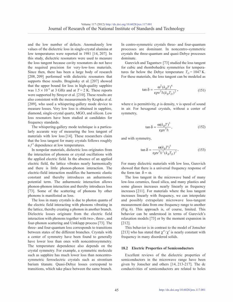
and the low number of defects. Anomalously lowvalues of the dielectric loss in single-crystal alumina atlow temperatures were reported in 1981 [14, 207]. Inthis study, dielectric resonators were used to measurethe loss tangent because cavity resonators do not havethe required precision for very-low-loss materials.Since then, there has been a large body of research[208, 209] performed with dielectric resonators thatsupports these results. Braginsky et al. [207] showedthat the upper bound for loss in high-quality sapphirewas 1.5 × 10–9 at 3 GHz and at T = 2 K. These reportswere supported by Strayer et al. [210]. These results arealso consistent with the measurements by Krupka et al.[209], who used a whispering-gallery mode device tomeasure losses. Very low loss is obtained in sapphire,diamond, single-crystal quartz, MGO, and silicon. Lowloss resonators have been studied at candidates forfrequency standards.

The whispering-gallery mode technique is a particu-larly accurate way of measuring the loss tangent ofmaterials with low loss [14]. These researchers claimthat the loss tangent for many crystals follows roughlya f 2 dependence at low temperatures.

In nonpolar materials, dielectric loss originates fromthe interaction of phonons or crystal oscillations withthe applied electric field. In the absence of an appliedelectric field, the lattice vibrates nearly harmonicallyand there is little phonon-phonon interaction. Theelectric-field interaction modifies the harmonic elasticconstant and thereby introduces an anharmonicpotential term. The anharmonic interaction allowsphonon-phonon interaction and thereby introduces loss[73]. Some of the scattering of phonons by otherphonons is manifested as loss.

The loss in many crystals is due to photon quanta ofthe electric field interacting with phonons vibrating inthe lattice, thereby creating a phonon in another branch.Dielectric losses originate from the electric fieldinteraction with phonons together with two-, three-, andfour-phonon scattering and Umklapp process [73]. Thethree- and four-quantum loss corresponds to transitionsbetween states of the different branches. Crystals witha center of symmetry have been found to generallyhave lower loss than ones with noncentrosymmetry.The temperature dependence also depends on thecrystal symmetry. For example, a symmetric moleculesuch as sapphire has much lower loss than noncentro-symmetric ferroelectric crystals such as strontiumbarium titanate. Quasi-Debye losses correspond totransitions, which take place between the same branch.

In centro-symmetric crystals three- and four-quantumprocesses are dominant. In noncentro-symmetriccrystals the three-quantum and quasi-Debye processesdominate.

Gurevich and Tagantsev [73] studied the loss tangentfor cubic and rhombohedric symmetries for tempera-tures far below the Debye temperature TD = 1047 K.For these materials, the loss tangent can be modeled as

(151)

where ε is permittivity, ρ is density, ν is speed of soundin air. For hexagonal crystals, without a center ofsymmetry,

(152)

and with symmetry,

(153)

For many dielectric materials with low loss, Gurevichshowed that there is a universal frequency response ofthe form tan δ ∝ ω.

The loss tangent in the microwave band of manylow-loss ceramics, fused silica, and many plastics andsome glasses increases nearly linearly as frequencyincreases [211]. For materials where the loss tangentincreases linearly with frequency, we can interpolateand possibly extrapolate microwave loss-tangentmeasurement data from one frequency range to another(Fig. 6). This approach is, of course, limited. Thisbehavior can be understood in terms of Gurevich’srelaxation models [73] or by the moment expansion in[212].

This behavior is in contrast to the model of Jonscher[213] who has stated that χ″ /χ′ is nearly constant withfrequency in many disordered solids.

18.2 Electric Properties of Semiconductors

Excellent reviews of the dielectric properties ofsemiconductors in the microwave range have beengiven by Jonscher and others [14, 213-217]. The dcconductivities of semiconductors are related to holes


45

4

5 2( )tan( )

B

B D

k Tk T

2ωδ =ερν

,

3

5( )tan ,Bk Tμ

ωδ =ε ν

5

5 2 2( )tan

( )B

B D

k Tk Tμ

ωδ =ε ν

.


and free charge. In the gigahertz region, the total loss inmost semiconductors decreases significantly since theeffects of the dc conductivity decreases; however, thedielectric component of loss increases. For galliumarsenide and gallium nitride the conductivity isrelatively low. Figure 18 shows measurement results onthe permittivity of high-resistivity gallium arsenide as afunction of frequency. These measurements were madeby a mode-filtered TE01 X-band cavity. Siliconsemiconductors can exhibit low to high loss dependingon the level of dopants in the material. There areSchottky barriers at the interface between semicon-ductors and metals and at p-n junctions that producelosses.

The conductivities of semiconductors at lowfrequencies fall between those of metals anddielectrics. The theory of conductivity of semiconduc-tors begins with an examination of the phenomena inintrinsic (undoped) samples. At temperatures above0 K, the kinetic (thermal) energy becomes sufficient toexcite valence band electrons into the conduction band,where an applied field can act upon them to produce acurrent. As these electrons move into the conductionband, holes are created in the valence band that effec-tively become another source of current. The totalexpression for the conductivity includes contributionsfrom both electrons and holes and is given byσdc = q (nμn + pμp ), where q is charge, n is the electrondensity, p is the hole density, and μn and μp are theelectron mobility and hole mobility, respectively.

In intrinsic semiconductors, the number of chargecarriers produced through thermal excitation is relative-ly small, but σdc can be significantly increased by

doping the material with small amounts of impurityatoms. These additional carriers require much lessthermal energy in order to contribute to σdc . Thisresults in more carriers becoming available as thetemperature increases, until ionization of all theimpurity atoms is complete.

For temperatures above the full ionization range ofthe dopants, σdc is increasingly dominated by μn and μp.In semiconductors such as silicon, the mobility of thecharge carriers decreases as the temperature increases,due primarily to the incoherent scattering of thecarriers with the vibrating lattice. At a temperature Ti ,intrinsic effects begin to contribute additional chargecarriers beyond the maximum contributions of theimpurity atoms, and σdc begins to increase again [215,216, 219-222].

19. Overview of the Interaction of RFFields With BiologicalMaterials

19.1 RF Electrical Properties of Cells, AminoAcids, Peptides, and Proteins

In this section, we will overview the dielectric relax-ation of cells, membranes, proteins, amino acids, andpeptides [97, 223-229]. This research area is very largeand we summarize only the most basic concepts as theyrelate to RF fields.

Dielectric response of biological tissues to appliedRF fields is related to membrane and cell boundaries,molecular dipoles, together with associated ionic fluidsand counterions [230]. The ionic solution produceslow-frequency losses that are very high. As a conse-quence of these mobile charge carriers, counterionsadhere to molecular surfaces, interface charge causesMaxwell-Wagner capacitances, and electrode polariza-tion is formed at electrode interfaces. All of theseprocesses can yield a very high effective ε′r at lowfrequencies. Some of the effects of the electrodes canbe corrected for by use of standard techniques [230,231] (Sec. 8).

Some biological tissues exhibit an α relaxation in the100 Hz to 1 kHz region due to dipoles and Maxwell-Wagner interface polarization, another β relaxation inthe megahertz region due to bound water, and γ relax-ation in the microwave region due to the relaxation ofwater and water that is weakly bond.

Amino acids contain carboxyl (COOH) groups,amide (NH2 ) groups, and side groups. The side groupsand the dipole moment of the amino and carboxylgroups determine most of the low-frequency dielectricproperties of the acid. Some of the side groups


46

Fig. 18. Relative permittivity ε′r of gallium arsenide measured by anX-band cavity [218]. Start, middle, and terminus refer to differentspecimens taken from the same boule. For these measurementsthe Type B expanded relative uncertainty at 10 GHz in ε′r wasU = kuc = 0.02 (k = 2), where k is coverage factor.


are polar, while others are nonpolar. When ionized, theamino and carboxyl groups have positive and negativecharges, respectively. This charge separation forms apermanent dipole (Fig. 5). α amino acids have anamino group and carboxyl group on the same carbondenoted Cα and α-amino acids have a dipole momentof 15 to 17 debyes (D) (1 debye equals 3.33 × 10–30

coulomb-meter). β amino acids have a CH2 groupbetween the amino and carboxyl groups, whichproduces a large charge separation and therefore adipole moment on the order of 20 D. For a very goodoverview see Pethig [223]. Peptides are formed fromcondensed amino acids. A peptide consists of a collec-tion of amino acids connected by peptide bonds.Peptide bonds provide connections to amino acidsthrough the CO-NH bond by means of the water mole-cule as a bridge. The peptide unit has a dipole momenton the order of 3.7 D. Chains of amino acids are calledpolyamino acids or polypeptides. These are terminatedby an amide group on one end and a carboxyl group onthe other side. Typical dipole moments for polypeptidesare on the order of 1000 D.

Polyamino acids can be either in the helical orrandom-coil phase. In the helical state, C = O bonds arelinked by hydrogen bonds to NH groups. The helix caneither be right-handed or left-handed; however, theright-handed helix is more stable. Generally, polyaminoacids have permanent dipole moments and dielectricrelaxation frequencies in the kilohertz region [232].

The origin of relaxation in proteins has been debatedover the years. Proteins are known to be composed ofpolyamino acids with permanent dipole moments, butthey also have free and loosely bound protons. Theseprotons bind loosely to the carboxyl and amino groups.Kirkwood et al. hypothesized that much of theobserved relaxation behavior of proteins is due to

movement of these nearly free protons in the appliedfield or the polarization of counterion sheaths aroundmolecules [233]. Strong protonic conductivity has alsobeen observed in DNA. At present, the consensus isthat polar side chains and both permanent dipoles andthe proton-induced polarization contribute to dielectricrelaxation of proteins.

In the literature three dielectric relaxations inproteins have been identified [231]. These are similarto that in DNA. The first is the α relaxation in the10 kHz to 1 MHz region and is due to rotation of theprotein side chains. The second minor β relaxationoccurs in the 100 MHz to 5 GHz range and is thoughtto be due to bound water. The third γ relaxation isaround 5 GHz to 25 GHz and is due to semi-free water.

Nucleic acids are high-molecular mass polymersformed of pyrimidine and purine bases, a sugar, andphosphoric-acid backbone. Nucleic acids are built up ofnucleotide units, which are composed of sugar, base,and phosphate groups in helical conformation.Nucleotides are linked by three phosphates groups,which are designated α, β, and γ . The phosphate groupsare linked through the pyrophosphate bond. Theindividual nucleotides are joined together by groups ofphosphates that form the phosphodiester bond betweenthe 3′ and 5′ carbon atoms of sugars. These phosphategroups are acidic. Polynucleotides have a hydroxylgroup at one end and a phosphate group on the otherend. Nucleosides are subunits of nucleotides andcontain a base and a sugar. The bond between the sugarand base is called the glycosidic bond. The base canrotate only in the possible orientations about theglycosidic bond.

Watson and Crick concluded through x-ray diffrac-tion studies that the structure of DNA is in the form ofa double-stranded helix. In addition to x-ray structureexperiments on DNA, information has been gleanedthrough nuclear magnetic resonance (NMR) experi-ments. Types A and B DNA are in the form of right-handed helices. Type Z DNA is in a left-handed confor-mation. There is a Type B to Z transition betweenconformations. A transition from Type A to Type BDNA occurs when DNA is dissolved in a solvent [234].The Watson-Crick conception of DNA as a uniformhelix is an approximation. In reality, DNA exists inmany conformations and may contain inhomogeneitiessuch as attached proteins. In general, double-strandedDNA is not a rigid rod, but rather a meandering chain.Once formed, even though the individual bondscomposing DNA are weak, the molecule as a whole isvery stable. The helical form of the DNA moleculeproduces major and minor grooves in the outer


47

Table 5. Approximate dipole moments

Material Dipole Moment (D)

H2O 1.85

CO 0.12

NaCl 9.00

Typical protein 500

Peptide 3.7

Amino acid 20

Polypeptide 1000


outer surface of the molecule. There are also bound-water molecules in the grooves. Many interactionsbetween proteins or protons with DNA occur in thesegrooves.

The helix is formed from two strands. The bases inadjacent strands combine by hydrogen bonding, anelectrostatic interaction with a pyrimidine on one sideand purine on the other. In DNA, the purine adenine(A) pairs with the pyrimidine thymine (T). The purineguanine (G) pairs with the pyrimidine cytosine (C). Ahydrogen bond is formed between a covalently bondeddonor hydrogen atom that is positively charged and anegatively charged acceptor atom. The A-T base pairassociates by two hydrogen bonds, whereas C-G basepairs associate by three hydrogen bonds. The base-pairsequence is the carrier of genetic information. Thegenetic code is formed of a sequence of three basepairs, which determine a type of amino acid. Forexample, the sequence of TTT AAA AAG GCT

determines an amino acid sequence of phenylalanine-lysine-lysine-alanine.

The DNA molecule has a net negative charge due tothe phosphate backbone. When dissolved in a cationsolution, some of the charge of the molecule is neutral-ized by cations. The double-stranded DNA molecule isgenerally thought to have little intrinsic permanentdipole moment. This is because the two strands thatcompose the helix are oriented so that the dipolemoment of one strand cancels the other. However,when DNA is dissolved in a solvent, such as salinesolution, an induced dipole moment forms due toreorganization of charge into a layer around themolecule called the counterion sheath.

The interaction of the counterions with biomoleculeshas been a subject of intensive research over the years.Some of the counterions bind to the phosphate back-bone with a weak covalent bond. Other counterions aremore loosely bound and some may penetrate into themajor and minor grooves of DNA [235]. Ions areassumed to be bound near charges in the DNA mole-cule, so that a double layer forms. The ions attracted tothe charged DNA molecule forms a counterion sheaththat shields some of the charge of the DNA. Thecounterion sheath around a DNA molecule is composedof cations such as Na or Mg, which are attracted to thebackbone negative phosphate charges. These chargesare somewhat mobile and oscillate about phosphatecharge centers in an applied electric field. A portion ofthese counterions is condensed near the surface of themolecule, whereas the vast majority are diffusely

bound. Double-stranded DNA possesses a largeinduced dipole moment on the order of thousands ofdebye, due to the counterion atmosphere. This factis gleaned from dielectric relaxation studies, birefrin-gence, and dichroism experiments [236], and otherlight-scattering experiments [237]. The induced dipolemoment μ→ in an electric field E is defined in terms ofthe polarizability μ→ = αE .

Because the individual strands of double-strandedDNA are antiparallel and the molecule is symmetrical,the transverse dipole moments should cancel. However,a number of researchers have measured a small perma-nent dipole moment for DNA [238]. In alternatingfields, the symmetry of the molecule may be deformedslightly to produce a small permanent dipole moment[231]. Another origin of the small permanent dipolemoment is attached charged ligands such as proteins ormultivalent cations [239]. These ligands produce a netdipole moment on the DNA molecule by breaking thesymmetry. The question of how much of the relaxationof the DNA molecule is due to induced dipolemomentversus permanent moment has been studied by Hoganet al. [236]. The response of permanent vs. induceddipole moment differs in terms of field strength. Thepotential energy of a permanent dipole moment atan angle θ to the electric field is U = – μ E cos θ,whereas the induced dipole moment in the electric fieldis quadratic, U = – (Δα /2)E 2 cos2 θ , where Δα is thedifference in polarizability along anisotropy axes of themolecule. Experiments indicate that the majority of themoment was induced rather than permanent. Chargetransport through DNA can be ballistic.

19.2 Dielectric Properties of BoundWater andPolyelectrolytes

Knowledge of the permittivity of the water near thesurface of a biomolecule is useful for modeling. Theregion close to a biomolecule in water has a relativelylow real part of permittivity and a fixed charge. Theregion far from the molecule has a permittivity closeto that of water. Lamm and Pack [240] studied thevariation of permittivity in the grooves, near the sur-face, and far away from the DNA molecule. The effec-tive permittivity depends on solvent concentration,distance from the molecule, the effects of the boundary,and dielectric field-saturation. The variation of permit-tivity with position significantly alters the predictionsfor the electric potential in the groove regions. Modelpredictions depend crucially on knowing the dielectricconstant of water. Numerical modeling of the DNAmolecule depends critically on the permittivity of


48

{{ { {

phe lyso lys ala


water. When the permittivity of water varies in space,numerical models indicate that small ions such as hydro-gen can penetrate into the minor and major grooves [235,241]. These predictions are not obtained for models thatuse spatially independent permittivity for water. Frommodeling results it was found that the real part of theeffective permittivity around the DNA molecule variesas a function of distance from the center of the mole-cule and as a function of solvent concentration in molesper liter (mol / l) [240].

The molecular structure of water is not simple.Besides the basic H2O triad structure of the watermolecule, there are also complicated hydrogen-bondednetworks created by dipole-dipole interactions thatform hydroxyl OH– and hydronium H3O+ ions. Thedielectric constant of water at low frequencies is about80, whereas biological water contains ions, whichaffect both the real and imaginary parts of the permit-tivity. Water bound in proteins and DNA has adecreased permittivity. This is due to constraints on themovement of the molecules when they are attached tobiomaterials.

19.3 Response of DNA and Other Biomolecules inElectric Driving Fields

The low-frequency response of DNA is due primarilyto longitudinal polarization of the diffuse counterionsheath that surrounds the molecule. This occurs atfrequencies in the range of 1 to 100 Hz. Another relax-ation occurs in the megahertz region due to movementof condensed counterions bound to individual phos-phate groups. Dielectric data on human tissue is givenin Figs. 19 and 20. A number of researchers havestudied dielectric relaxation of both denatured andhelical conformation DNA molecules in electrolytesolutions both as a function of frequency and appliedfield strength. Single-stranded DNA exhibited lessdielectric relaxation than double-stranded DNA [98,243-246]. Takashima concluded that denatured DNAtended to coil and thereby decrease the effective lengthand therefore the dipole moment. Furthermore, a highelectric field strength affects DNA conductivity in twoways [244]. First, it promotes an increased dissociationof the molecule and thereby increases conductivity.Second, it promotes an orientation field effect wherealignment of polyions increases conductivity.

There are many other types of motion of the DNAmolecule when subjected to mechanical or millimeteror terahertz electrical driving fields. For example,propeller twist occurs when two adjacent bases in a pairtwist in opposite directions. Another motion is the

breather mode where two bases oscillate in oppositionas hydrogen bonds are compressed and expanded. TheLippincott-Schröder and Lennard-Jones potentials arecommonly used for modeling these motions. Thesemodes resonate at wavelengths in the millimeterregion; however, relaxation damping prevents directobservation. Other static or dynamic motions of thebase pairs of the DNA molecule are roll, twist, andslide.

Single-stranded DNA, in its stretched state, possess-es a dipole moment oriented more or less transverse tothe axis. The phosphate group produces a permanenttransverse dipolemoment of about 20 D per 0.34 nmbase-pair section. The Debye (D) is a unit of dipolemoment and has a value of 3.336 × 10–30 C . m.Because the typical DNA molecule contains thousandsof base pairs, the net dipole moment can be significant.However, as the molecule coils or the base pairs twist,the dipole moment decreases. If single strands ofDNA were rigid, since there is a transverse dipolemoment, and relaxation would occur in the megahertzto gigahertz frequencies.


49

Fig. 19. Measurements of the relative permittivity of various bodytissues by Gabriel et al. [242] (no uncertainties assigned).

Fig. 20. Loss tangent of human tissues by Gabriel et al. [242].


19.4 Dynamics of Polarization Relaxation inBiomaterials

In order to study relaxation of polypeptides andDNA in solution, we first consider the simplest modelof a dipolar rigid rod.

The torque on an electric dipole moment p is

(154)

For cases where the dipole moment is perpendicularto the rod axis, rotations about the major axis can occur.The longitudinal rotation relaxation time for a moleculeof length L is given in [247]. The relaxation time varieswith the molecule length. Major axis rotation couldoccur if the molecule had a transverse dipole moment;for example, in a single strand of DNA.

When the dipole moment is parallel to the majoraxis, end-over-end rotation may occur. This is the typeof relaxation at low frequencies that occurs with theinduced dipole moment in the counterion sheath or apermanent dipole moment parallel to the longitudinalaxis of the molecule. The relaxation time varies as L3.Because length of the molecule and molecular mass arerelated, the responses for the two relaxations depend onmolecular mass. Also, the model presented in thissection assumes the rod is rigid. In reality, DNA is notrigid, so a statistical theory of relaxation needs to beapplied [247-249].

Takashima [98] and Sakamoto et al. [243] havederived a more comprehensive theory for counterionrelaxation and found that the relaxation time varies inproportion to the square of the length of the molecule[249, 250]. Most experimental evidence indicates a L2

dependence. This is in contrast to the rigid-rod modelwhere the relaxation time varies as L3.

19.5 Counterion Interaction With DNA and Proteins

The real and imaginary parts of permittivity dependon the concentration and type of cations [250]. As theconcentration of the solvent increases, more of thephosphate charge is neutralized and the dielectricincrement (difference between the permittivity of themixture and solvent by itself) decreases.

Many types of cations compounds have been usedin DNA solvents; for example, NaCl, LiCl, AgNO2 ,CuCl2 , MnCl2 , MgCl2 , arginines, protamine, dyes,lysine, histones, and divalent metals such as Pb, Cd, Ni,Zn, and Hg [243, 251-253]. The simple inorganic-monovalent cations bind to the DNA molecule nearthe phosphate backbone to form both a condensed anddiffuse sheath. There is evidence that strong concen-

trations of divalent metal cations destabilize the DNAhelix [254]. Sakamoto et al. [252] found that the dielec-tric increment decreased for divalent cations.

On the other hand, histones and protamines tightlybind in the major groove of the DNA molecule. Theyproduce stability in the double helix by neutralizingsome of the phosphate charge. Dyes can attach to DNA,neutralize charge, and thereby decrease dielectricincrement.

20. Methods for Modeling Electro-magnetic Interactions With Bio-molecules, Nanoprobes, andNanowires

Modeling methods for EM interactions with materi-als include solving mode-match solutions to Maxwell’sequations, finite-element and molecular dynamics simulations, and finite-difference time-domain models.Finite-element modeling software can solve Maxwell’sequations for complicated geometries and small-scalesystems.

Traditionally, mode-match solutions to Maxwell’sequations meant solving Maxwell’s equations in eachregion and then matching the modal field componentsat the interfaces and requiring, by the boundaryconditions, all the tangential electric fields go to zeroon conductors. On the nanoscale, the microwave andmillimeter wavelengths are much larger than thefeature size; the skin depths are usually larger than thedevice being measured. Therefore modes must bedefined both outside the nanowire and inside the wireand matched at the interface. Also, the role of the nearfield is more important.

The EM model for a specific problem must capture theimportant physics such as skin depth, ballistictransport, conductor resistance, and quantized capaci-tance, without including all of the microstructuralcontent. Modeling nanoscale electromagnetics isparticularly difficult in that quantum effects cannotalways be neglected; however, the EM field in thesemodels is usually treated classically. In the case of near-field probes the skin depths are usually larger than thewire dimensions, and therefore the fields then need to bedetermined in both the wire and in the space surroundingthe wire. Sommerfeld and Goubau surface waves andplasmons propagate at the interface of dielectric andfinite conductivity metals and need to be taken intoaccount in modeling probe interactions. The probe-material EM communication is often transmitted by thenear field.


50

= .×N p E


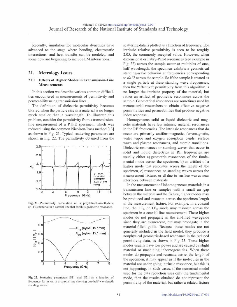
Recently, simulators for molecular dynamics haveadvanced to the stage where bonding, electrostaticinteractions, and heat transfer can be modeled, andsome now are beginning to include EM interactions.

21. Metrology Issues21.1 Effects of Higher Modes in Transmission-Line

Measurements

In this section we describe various common difficul-ties encountered in measurements of permittivity andpermeability using transmission lines.

The definition of dielectric permittivity becomesblurred when the particle size in a material is no longermuch smaller than a wavelength. To illustrate thisproblem, consider the permittivity from a transmission-line measurement of a PTFE specimen, which wasreduced using the common Nicolson-Ross method [13]as shown in Fig. 21. Typical scattering parameters areshown in Fig. 22. The permittivity obtained from the

scattering data is plotted as a function of frequency. Theintrinsic relative permittivity is seen to be roughly2.05, the commonly accepted value. However, whendimensional or Fabry-Perot resonances (see example inFig. 22) across the sample occur at multiples of one-half wavelength, the specimen exhibits a geometricalstanding-wave behavior at frequencies correspondingto nλ /2 across the sample. So if the sample is treated asa single particle at these standing wave frequencies,then the “effective” permittivity from this algorithm isno longer the intrinsic property of the material, butrather an artifact of geometric resonances across thesample. Geometrical resonances are sometimes used bymetamaterial researchers to obtain effective negativepermittivities and permeabilities that produce negativeindex response.

Homogeneous solid or liquid dielectric and mag-netic materials have few intrinsic material resonancesin the RF frequencies. The intrinsic resonances that dooccur are primarily antiferromagnetic, ferromagnetic,water vapor and oxygen absorption bands, surfacewave and plasma resonances, and atomic transitions.Dielectric resonances or standing waves that occur insolid and liquid dielectrics in RF frequencies areusually either a) geometric resonances of the funda-mental mode across the specimen, b) an artifact of ahigher mode that resonates across the length of thespecimen, c) resonances or standing waves across themeasurement fixture, or d) due to surface waves nearinterfaces between materials.

In the measurement of inhomogeneous materials in atransmission line or samples with a small air gapbetween the material and the fixture, higher modes maybe produced and resonate across the specimen lengthin the measurement fixture. For example, in a coaxialline, the TE0n or TE11 mode may resonate across thespecimen in a coaxial line measurement. These highermodes do not propagate in the air-filled waveguidesince they are evanescent, but may propagate in thematerial-filled guide. Because these modes are notgenerally included in the field model, they produce anonphysical geometric-based resonance in the reducedpermittivity data, as shown in Fig. 25. These highermodes usually have low power and are caused by slightmaterial or machining inhomogeneities. When thesemodes do propagate and resonate across the length ofthe specimen, it may appear as if the molecules in thematerial are under going intrinsic resonance, but this isnot happening. In such cases, if the numerical modelused for the data reduction uses only the fundamentalmode, then the results obtained do not represent thepermittivity of the material, but rather a related fixture


51

Fig. 21. Permittivity calculation on a polytetrafluoroethylene(PTFE) material in a coaxial line that exhibits geometric resonance.

Fig. 22. Scattering parameters |S11| and |S21| as a function offrequency for nylon in a coaxial line showing one-half wavelengthstanding waves.


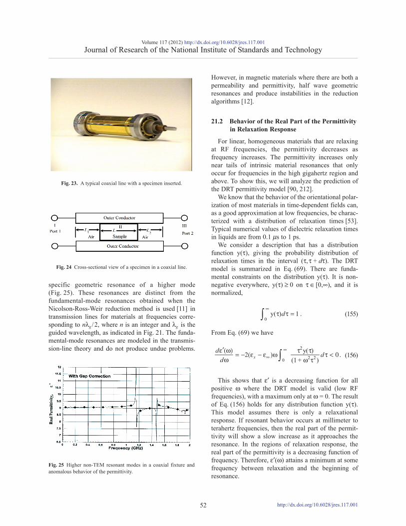
specific geometric resonance of a higher mode(Fig. 25). These resonances are distinct from thefundamental-mode resonances obtained when theNicolson-Ross-Weir reduction method is used [11] intransmission lines for materials at frequencies corre-sponding to nλg /2, where n is an integer and λg is theguided wavelength, as indicated in Fig. 21. The funda-mental-mode resonances are modeled in the transmis-sion-line theory and do not produce undue problems.

However, in magnetic materials where there are both apermeability and permittivity, half wave geometricresonances and produce instabilities in the reductionalgorithms [12].

21.2 Behavior of the Real Part of the Permittivityin Relaxation Response

For linear, homogeneous materials that are relaxingat RF frequencies, the permittivity decreases asfrequency increases. The permittivity increases onlynear tails of intrinsic material resonances that onlyoccur for frequencies in the high gigahertz region andabove. To show this, we will analyze the prediction ofthe DRT permittivity model [90, 212].

We know that the behavior of the orientational polar-ization of most materials in time-dependent fields can,as a good approximation at low frequencies, be charac-terized with a distribution of relaxation times [53].Typical numerical values of dielectric relaxation timesin liquids are from 0.1 μs to 1 ps.

We consider a description that has a distributionfunction y(τ), giving the probability distribution ofrelaxation times in the interval (τ,τ + dτ). The DRTmodel is summarized in Eq. (69). There are funda-mental constraints on the distribution y(τ). It is non-negative everywhere, y(τ) ≥ 0 on τ ∈ [0,∞), and it isnormalized,

(155)

From Eq. (69) we have

(156)

This shows that ε′ is a decreasing function for allpositive ω where the DRT model is valid (low RFfrequencies), with a maximum only at ω = 0. The resultof Eq. (156) holds for any distribution function y(τ).This model assumes there is only a relaxationalresponse. If resonant behavior occurs at millimeter toterahertz frequencies, then the real part of the permit-tivity will show a slow increase as it approaches theresonance. In the regions of relaxation response, thereal part of the permittivity is a decreasing function offrequency. Therefore, ε′(ω) attains a minimum at somefrequency between relaxation and the beginning ofresonance.


52

Fig. 23. A typical coaxial line with a specimen inserted.

Fig. 24 Cross-sectional view of a specimen in a coaxial line.

Fig. 25 Higher non-TEM resonant modes in a coaxial fixture andanomalous behavior of the permittivity.

0y( )d

∞τ τ = 1 .∫

0

y( )2( )(1 + )

2∞∞ 2 2

′ε (ω) τ τ= − ε − ε ω τ < 0.ω ω τ∫s

d dd


22. Permittivity Mixture Equations

We can readily estimate the permittivity of a mixtureof a number of distinct materials. The effective permit-tivity of a mixture εe f f of constituents with permittivi-ties ei and volume fractions θi can be approximated invarious ways. The Bruggeman equation [256] is usefulfor binary mixtures:

(157)

or the Maxwell-Garnett mixture equation [256] can beused:

(158)

where ε′1 is the permittivity of the matrix and ε′2 isthe permittivity of the filler [257]. The formula byLichtenecker is for a powerlaw dependence of thereal part of the permittivity for –1 ≤ k ≤ 1, and wherethe volume fractions of the inclusions and host areνp and νm :

(159)

This equation has successfully modeled compositeswith random inclusions embedded into a host. Anapproximation to this is

(160)

23. Discussion

The broad area of RF dielectric electromagneticinteractions with solid and liquid materials from themacroscale down to the nanoscale materials wasoverviewed. The goal was to give a researcher a broadoverview and access to references in the various areas.The paper studied the categories of electromagneticfields, relaxation, resonance, susceptibility, linearresponse, interface phenomena, plasmons, the conceptsof permittivity and permeability, and relaxation times.Topics of current research interest, such as plasmonicbehavior, negative-index behavior, noise, heating,

nanoscale materials, wave cloaking, polariton surfacewaves, biomaterials, and other topics were covered.The definition and limitations of the concept of permit-tivity in materials was discussed. We emphasized thatthe permittivity and permeability are well defined whenthe applied field has a wavelength much longer than theeffective particle size in the material and when multiplescattering between inclusions is minimal as the wavepropagates through the material. In addition, the use ofthe concept of permittivity requires an ensemble ofparticles that each have dielectric response.

Acknowledgements

We acknowledge discussions with team members ofthe Innovation Measurements Science Program atNIST: Detection of Corrosion in Steel-ReinforcedConcrete by Antiferromagnetic Resonance, discussionswith Nick Paulter of OLES, and Pavel Kabos and manyother over the years.

24. References

[1] NTIA United States Frequency Allocation Chart,http://www.ntia.doc.gov/osmhome/allochrt.pdf.

[2] C. Roychoudhuri, A. F. Kracklauer, and K. Creath, The natureof light: What is a photon, CRC Press, NY (2008).http://dx.doi.org/10.1201/9781420044256

[3] K. Horie, H. Ushiki, and F. M. Winnik, Molecular Photonics,Wiley, NY (2000). http://dx.doi.org/10.1002/9783527613205

[4] C. Kittel, Introduction to Solid State Physics, 6th Edition, JohnWiley, NY (1986).

[5] N. W. Ashcroft and N. D. Mermim, Solid State Physics,Saunders College, Philadelphia (1976).

[6] G. Smith, Introduction to Classical Electromagnetic Radiation,Cambridge University Press, Cambridge, UK (1997).

[7] S. Yang, G. Beach, C. Knutson, D. Xiao, Q. Niu, M. Tsoi, andJ. Erskine, Universal electromotive force induced by domainwall motion, Phys. Rev. Lett. 102, 067201 (2009).http://dx.doi.org/10.1103/PhysRevLett.102.067201

[8] J. C. Slonczewski, Current-driven excitation of magnetic mul-tilayers, J. Magn. Magn. Mater. 159, L1-L7 (1996).http://dx.doi.org/10.1016/0304-8853(96)00062-5

[9] L. Berger, Emission of spin waves by a magnetic multilayertraversed by a current, Phys. Rev B 54, 9353-9358 (1996).http://dx.doi.org/10.1103/PhysRevB.54.9353

[10] R. Clarke, A guide to the dielectric characterization of materi-als in rf and microwave frequencies, Best Practice Guide, UK(2003).

[11] J. Baker-Jarvis, R. G. Geyer, and P. D. Domich, A non-linearleast-squares solution with causality constraints applied totransmission line permittivity and permeability determination,IEEE Trans. Instrum. Meas. 41, 646-652 (1992).http://dx.doi.org/10.1109/19.177336

[12] J. Baker-Jarvis, M. D. Janezic, J. H. Grosvenor, and R. G.Geyer, Transmission/Reflection and Short-Circuit Line


53

2 2e f f e f f

e f f e f f

1 21 2

1 2

′ ′ ′ ′ε − ε ε − εθ = θ

′ ′ ′ ′ε + ε ε + ε,

2

2 22 2e f f

e f f

2 11

1

′ ′ε − ε ′ ′ε − ε= θ′ ′ ′ ′ε + ε ε + ε

,

.k k kp p m mν νε = ε + ε

ln = ln lnp p m m .V Vε ε + ε


Methods for Measuring Permittivity and Permeability, NISTTech. Note 1355 (1992).

[13] J. Baker-Jarvis, Transmission/Reflection and Short-CircuitLine Permittivity Measurements, NIST Tech. Note 1341(1990).

[14] J. Baker-Jarvis, M. D. Janezic, B. Riddle, C. L. Holloway,N. G. Paulter, and J. E. Blendell, Dielectric and conductor-losscharacterization and measurements on electronic packagingmaterials, NIST Tech. Note 1520 (2001).

[15] J. Baker-Jarvis, M. D. Janezic, B. Riddle, P. Kabos, R. Johnk,C. Holloway, R. Geyer, and C. Grosvenor, Measuring the per-mittivity and permeability of lossy materials: Solids, liquids,metals, building materials, and negative-index materials,NIST Tech. Note 1536 (2005).

[16] M. D. Janezic and J. Baker-Jarvis, Permeability of Metals,NIST Tech. Note 1532 (2004).

[17] S. M. Rytov, Y. A. Kravtsov, and V. I. Tatarski, Principles ofStatistical Radiophysics, Vol. 3, Springer-Verlag, Moscow(1978).

[18] K. Joulain, J. P. Mulet, F. Marquier, R. Carminati, and J. J.Greffet, Surface electromagnetic waves thermally excited:Radiative heat transfer, coherence properties and Casimirforces revisited in the near field, Surf. Sci. Rep. 57, 59-112(2005). http://dx.doi.org/10.1016/j.surfrep.2004.12.002

[19] J. Baker-Jarvis, Time-dependent entropy evolution in micro-scopic and macroscopic electromagnetic relaxation, Phys.Rev. E 72, 066613 (2005).http://dx.doi.org/10.1103/PhysRevE.72.066613

[20] J. Baker-Jarvis, M. D. Janezic, and D. C. deGroot, Tutorial onhigh frequency dielectric measurements, IEEEInstrumentation and Measurements Magazine 13, 24-31(2010). http://dx.doi.org/10.1109/MIM.2010.5438334

[21] H. Schwan, Interactions between electromagnetic fields andcells, Plenum Press, NY, pp. 371-389 (1985).

[22] A.W. Friend, E. D. Finch, and H. P. Schwan, Low frequencyelectric field induced changes in the shape and mobility ofamoebae, Science 187, 357-359 (1975).http://dx.doi.org/10.1126/science.1111109

[23] T. J. Lewis, Interfaces are the dominant features of dielectricsat the nanometric level, IEEE Trans. Dielectr. Electr. Insul. 11,739-753 (2004).http://dx.doi.org/10.1109/TDEI.2004.1349779

[24] S. Ramo, J. R. Whinnery, and T. V. Duzer, Fields and Waves inCommunication Electronics, John Wiley and Sons, NY(1984).

[25] P. J. Mohr, B. N. Taylor, and D. B. Newell, CODATA recom-mended values of the fundamental physical constants: 2006,Rev. Mod. Phys. 80, 633 (2008).http://dx.doi.org/10.1103/RevModPhys.80.633

[26] V. G. Veselago, The electrodynamics of substances with simul-taneously negative values of ε and μ, Soviet Phys. Usp. 10,509-514 (1968).http://dx.doi.org/10.1070/PU1968v010n04ABEH003699

[27] J. D. Jackson, Classical Electrodynamics (3rd Ed.), John Wileyand Sons, NY (1999).

[28] D. Kajfez, Q Factor, Vector Fields, US (1994).[29] P. Mazur and B. R. A. Nijboer, On the statistical mechanics of

matter in an electromagnetic field: I, Physica 19, 971-986(1953). http://dx.doi.org/10.1016/S0031-8914(53)80109-6

[30] F. N. H. Robinson, Macroscopic Electromagnetism, PergamonPress, Oxford (1973).

[31] S. R. de Groot and L. G. Suttorp, Foundations ofElectrodynamics, American Elsevier, NY (1972).

[32] R. E. Raab and J. H. Cloete, An eigenvalue theory of circularbirefringence and dichroism in a non-magnetic chiral medium,J. Electromagnetic Waves and Applications 8, 1073-1089(1994). http://dx.doi.org/10.1163/156939394X00759

[33] F. Bloch and A. Siegert, Magnetic resonance for nonrotatingfields, Phys. Rev. 57, 522 (1940).http://dx.doi.org/10.1103/PhysRev.57.522

[34] C. Kittel, On the theory of ferromagnetic absorption, Phys.Rev. 73, 155-161 (1948).http://dx.doi.org/10.1103/PhysRev.73.155

[35] H. B. Callen, A ferromagnetic dynamical equation, J. Phys.Chem. Solids 4, 256-270 (1958).http://dx.doi.org/10.1016/0022-3697(58)90077-5

[36] N. Bloembergen, On the ferromagnetic resonance in nickeland Supermalloy, Phys. Rev. 78, 572-580 (1950).http://dx.doi.org/10.1103/PhysRev.78.572

[37] J. H. van Vleck, Concerning the theory of ferromagneticabsorption, Phys. Rev. 78, 266-274 (1950).http://dx.doi.org/10.1103/PhysRev.78.266

[38] D. F. Nelson, Electric, Optic, and Acoustic Interactions inDielectrics, John Wiley and Sons, NY (1979).

[39] R. Loudon, L. Allen, and D. F. Nelson, Propagation of electro-magnetic energy and momentum in absorbing dielectric, Phys.Rev. A 52, 1071-1085 (1997).

[40] J. Baker-Jarvis, P. Kabos, and C. L. Holloway, Nonequilibriumelectromagnetics: Local and macroscopic fields using statisti-cal mechanics, Phys. Rev. E 70, 036615 (2004).http://dx.doi.org/10.1103/PhysRevE.70.036615

[41] J. Baker-Jarvis, A general dielectric polarization evolutionequation, IEEE Trans. Dielectr. Electr. Insul. 7, 374-384(2000). http://dx.doi.org/10.1109/94.848919

[42] E. B. Graham, J. Pierrus, and R. E. Raab, Multipole momentsand Maxwell’s equations, J. Phys. B 25, 4673-4684 (1992).http://dx.doi.org/10.1088/0953-4075/25/21/030

[43] J. Baker-Jarvis, P. Kabos, Dynamic constitutive relations forpolarization and magnetization, Phys. Rev. E 64, (2001)56127. http://dx.doi.org/10.1103/PhysRevE.64.056127

[44] J. Baker-Jarvis, Electromagnetic nanoscale metrology basedon entropy production and fluctuations, Entropy 10, 411-429(2008). http://dx.doi.org/10.3390/e10040411

[45] B. Robertson, Equations of motion of nuclear magnetism,Phys. Rev. 153, 391-403 (1967).http://dx.doi.org/10.1103/PhysRev.153.391

[46] J. Baker-Jarvis, M. D. Janezic, and B. Riddle, Dielectric polar-ization equations and relaxation times, Phys. Rev. E 75,056612 (2007).http://dx.doi.org/10.1103/PhysRevE.75.056612

[47] A. Alu, M. Silveirinha, A. Salandrino, and N. Engheta,Epsilonnear- zero metamaterials and electromagnetic sources:tailoring the radiation phase pattern, Phys. Rev. B 75, 155410(2007). http://dx.doi.org/10.1103/PhysRevB.75.155410

[48] F. deFornel, Evanescent waves from Newtonian optics toatomic optics, Springer, Berlin (2000).

[49] Y. K. Yoo and X. D. Xiang, Combinatorial material prepara-tion, J. Phys. Condensed Matter 14, R49-R78 (2002).http://dx.doi.org/10.1088/0953-8984/14/2/202

[50] M. Janezic, J. Jargon, and J. Baker-Jarvis, Relative permittivi-ty measurements using the higher-order resonant mode of anearfield microwave probe, in: URSI Proceedings, Chicago,IL (2008).

[51] P T. van Duijnen, A. H. de Vries, M. Swart, and F. Grozema,Polarizabilities in the condensed phase and the local fields



problem: A direct field formulation, J. Chem. Phys. 117, 8442-8453 (2002). http://dx.doi.org/10.1063/1.1512278

[52] R. Wortmann and D. M. Bishop, Effective polarizabilities andlocal field corrections for nonlinear optical experiments incondensed media, J. Chem. Phys. 108, 1001 (1998).http://dx.doi.org/10.1063/1.475462

[53] C. J. F. Bottcher and P. Bordewijk, Theory of ElectricPolarization, Vol. I and II, Elsevier, NY (1978).

[54] M. Mandel and P. Mazur, On the molecular theory of dielectricrelaxation, Physica 24, 116-128 (1958).http://dx.doi.org/10.1016/S0031-8914(58)94005-9

[55] J. E. Gubernatis, Scattering theory and effective mediumapproximations to heterogeneous materials, AIP 1stConference on Electrical Transport and Optical Properties ofInhomogeneous Materials, 84-98 (1978).

[56] O. Keller, Local fields in the electrodynamics of mesoscopicmedia, Physics Reports 268, 85-262 (1996).http://dx.doi.org/10.1016/0370-1573(95)00059-3

[57] R. H. Cole, Correlation function theory of dielectric relax-ation, J. Chem. Phys. 42, 637-643 (1965).http://dx.doi.org/10.1063/1.1695984

[58] S. E. Schnatterly and C. Tarrio, Local fields in solids: aspectsfor dielectrics, Rev. Mod. Phys. 64, 619-622 (1992).http://dx.doi.org/10.1103/RevModPhys.64.619

[59] M. Kuhn and H. Kliem, Local field in dielectric nanospheresfrom a microscopic and macroscopic point of view, IEEETrans. Dielectr. Electr. Insul. 16, 596-600 (2009).http://dx.doi.org/10.1109/TDEI.2009.5128493

[60] D. Mcquarrie, Statistical Mechanics, University ScienceBooks, NY (2000).

[61] J. Baker-Jarvis and J. Surek, Transport of heat and charge inelectromagnetic metrology based on nonequilibrium statisticalmechanics, Entropy 11, 748-765 (2009).http://dx.doi.org/10.3390/e11040748

[62] C. L. Holloway, E. F. Kuester, J. Baker-Jarvis, and P. Kabos, Adouble negative (DNG) composite material composed of mag-netodielectric spherical particles in a dielectric, IEEE Trans.Antennas Propag. 51, 2596-2603 (2003).http://dx.doi.org/10.1109/TAP.2003.817563

[63] J. B. Pendry, A. J. Holden, D. J. Robbins, and W. J. Stewart,Magnetism from condctors and enhanced nonlinear phenome-na, IEEE Trans. Microwave Theory Tech. 47, 2075-2084(1999). http://dx.doi.org/10.1109/22.798002

[64] J. B. Pendry, A. J. Holden, W. J. Stewart, and I. Youngs,Extremely low frequency plasmons in metallic mesostruc-tures, Phys. Rev. Lett. 76, 4773-4776 (1996).http://dx.doi.org/10.1103/PhysRevLett.76.4773

[65] J. B. Pendry, A. J. Holden, D. J. Robbins, and W. J. Stewart,Low frequency plasmons on thin-wire structures, J. Phys.:Condens. Matter 10, 4785-4809 (1998).http://dx.doi.org/10.1088/0953-8984/10/22/007

[66] R. W. Ziolkowski and E. Heyman, Wave propagation in mediahaving negative permittivity and permeability, Phys. Rev. E64, 056625-1:15 (2001).

[67] C. R. Simovski, Material parameters of metamaterials (aReview), Optics and Spectroscopy 107, 726-753 (2009).http://dx.doi.org/10.1134/S0030400X09110101

[68] C. L. Holloway, M. Mohamed, E. Kuester, and A. Dienstfrey,Reflection and transmission properties of a metafilm: With anapplication to a controllable surface composed of resonantparticles, IEEE Trans. Electromagnetic Compatibility 47, 853-865 (2005). http://dx.doi.org/10.1109/TEMC.2005.853719

[69] S. Kim, E. F. Kuester, C. L. Holloway, A. D. Scher, and J.Baker-Jarvis, Boundary effects on the determination of meta-material parameters from normal incidence reflection andtransmission measurements, IEEE Trans. Antennas Propag.59, 2226-2240 (2011).http://dx.doi.org/10.1109/TAP.2011.2143679

[70] K. Henneberger, Additional boundary conditions: An historicalmistake, Phys. Rev. Lett. 80, 2889-2892 (1998).http://dx.doi.org/10.1103/PhysRevLett.80.2889

[71] K. Mauritz, http://www.psrc.usm.edu/mauritz/mauritz.html.[72] G. G. Raju, Dielectrics in Electric Fields, 1st Edition, Marcel-

Dekker, Inc., NY (2003).http://dx.doi.org/10.1201/9780203912270

[73] V. L. Gurevich and A. K. Tagantsev, Intrinsic dielectric loss incrystals, Advances in Physics 40, 719-767 (1991).http://dx.doi.org/10.1080/00018739100101552

[74] V. L. Gurevich, Dielectric loss in crystals, Sov. Phys. SolidState 21, 1993-1998 (1979).

[75] L. A. Dissado and R. M. Hill, Anomalous low frequency dis-persion, Chem. Soc. Faraday Trans. 2 80, 291-318 (1984).

[76] H. Scher and E. W. Montroll, Anomalous transient-time dis-persion in amorphous solids, Phys. Rev. B12, 2455-2477(1975). http://dx.doi.org/10.1103/PhysRevB.12.2455

[77] A. Hunt, Comment on “A probabilistic mechanism hiddenbehind the universal power law for dielectric relaxation: gen-eral relaxation equation,” J. Phys. Condens. Matter 4, 10503-10512 (1992). http://dx.doi.org/10.1088/0953-8984/4/50/040

[78] A. K. Jonscher, The universal dielectric response and its phys-ical significance, IEEE Trans. Dielectr. Electr. Insul. 27, 407-423 (1992).

[79] L. A. Dissado and R. M. Hill, The fractal nature of the clustermodel dielectric response functions, J. Appl. Phys. 66, 2511-2524 (1989). http://dx.doi.org/10.1063/1.344264

[80] A. K. Jonscher, A many-body model of dielectric polarizationin solids, Phys. Stat. Sol. (b) 83, 585-597 (1977).http://dx.doi.org/10.1002/pssb.2220830227

[81] J. E. Anderson, Model calculations of cooperative motions inchain molecules, J. Chem. Phys. 52, 2821-2830 (1970).http://dx.doi.org/10.1063/1.1673406

[82] R. H. Cole, Molecular correlation function approaches todielectric relaxation, in: Physics of Dielectric Solids, Instituteof Physics, Cambridge, MA, pp. 1-21 1980.

[83] J. E. Shore and R. Zwanzig, Dielectric relaxation and dynam-ic susceptibility of one-dimension model for perpendicular-dipole polymers, J. Chem. Phys. 63, 5445-5458 (1975).http://dx.doi.org/10.1063/1.431279

[84] A. Papoulis, The Fourier Integral and Its Applications,McGraw-Hill, New York (1987).

[85] L. Fonda, G. C. Ghirardi, and A. Rimini, Decay theory ofunstable quantum systems, Rep. Prog. Phys. 41, 587-631(1978). http://dx.doi.org/10.1088/0034-4885/41/4/003

[86] R. R. Nigmatullin, Theory of the dielectric relaxation in non-crystalline solids: from a set of micromotions to the averagedcollective motion in the mesoscale region, Physica B 358,201-215 (2005).http://dx.doi.org/10.1016/j.physb.2005.01.173

[87] R. R. Nigmatullin and S. O. Nelson, New quantitative readingof dielectric spectra of complex biological systems, IEEETrans. Dielectr. Electr. Insul. 13, 1325-1334 (2006).http://dx.doi.org/10.1109/TDEI.2006.258204

[88] J. Baker-Jarvis, M. D. Janezic, and J. H. Lehmann, Dielectricresonator method for measuring the electrical conductivity of



carbon nanotubes from microwave to millimeter frequencies,J. Nanomaterials 2007, 24242 (2007).http://dx.doi.org/10.1155/2007/24242

[89] B. Robertson, Equations of motion in nonequilibrium statisti-cal mechanics, Phys. Rev. 144, 151-161 (1966).http://dx.doi.org/10.1103/PhysRev.144.151

[90] M. W. Coffey, On the generic behavior of the electrical permit-tivity at low frequencies, Phys. Lett. A. 373, 2793-2795(2009). http://dx.doi.org/10.1016/j.physleta.2009.05.069

[91] K. K. Mei and G. C. Liang, Electromagnetics of superconduc-tors, IEEE Trans. Microwave Theory Tech. 39, 1545–1552(1991). http://dx.doi.org/10.1109/22.83830

[92] B. Meng, B. D. B. Klein, J. H. Booske, and R. F. Cooper,Microwave absorption in insulating dielectric ionic crystalsincluding the role of point defects, Phys. Rev. B 53, 12777-12785 (1996). http://dx.doi.org/10.1103/PhysRevB.53.12777

[93] J. C. Dyre and T. B. Schroder, Universality of ac conduction indisordered solids, Rev. Mod. Phys. 72, 873-892 (2000).http://dx.doi.org/10.1103/RevModPhys.72.873

[94] S. A. Rozanski and F. Kremer, Relaxation and charge transportin mixtures of zwitter-ionic polymers and inorganic salts,Macromol. Chem. Phys. 196, 877-890 (1995).http://dx.doi.org/10.1002/macp.1995.021960316

[95] H. P. Schwan, Linear and nonlinear electrode polarization andbiological materials, Ann. Biomed. Eng. 20, 269-288 (1992).http://dx.doi.org/10.1007/BF02368531

[96] J. Baker-Jarvis, B. Riddle, and A. Young, Ion dynamics nearcharged electrodes with excluded volume effect, IEEE Trans.Dielectr. Electr. Insul. 6, 226-235 (1999).http://dx.doi.org/10.1109/94.765913

[97] R. H. French, Long range interactions in nanoscale science,Rev. Mod. Phys. 82, 1887-1944 (2007).http://dx.doi.org/10.1103/RevModPhys.82.1887

[98] S. Takashima, Dielectric dispersion of deoxyribonucleic acid,J. Phys. Chem. 70, 1372-1379 (1966).http://dx.doi.org/10.1021/j100877a006

[99] H. P. Schwan, Electrical properties of tissue and cell suspen-sions, in: Advances in Biological and Medical Physics, J.Laurence and C. A. Tobias (Eds.), Academic Press, pp. 147-209 (1957).

[100] J. C. Bernengo and M. Hanss, Four-electrode, very-low-fre-quency impedance comparator for ionic solutions, Rev. Sci.Instrum. 47, 505-508 (1976).http://dx.doi.org/10.1063/1.1134664

[101] A. Ben-Menahem and S. J. Singh, Seismic Waves and Sources,Springer-Verlag, NY (1981).http://dx.doi.org/10.1007/978-1-4612-5856-8

[102] I. Bunget and M. Popescu, Physics of Solid Dielectrics,Elsevier, NY (1984).

[103] R. Kono, T. A. Litovitz, and G. E. McDuffie, Comparison ofdielectric and mechanical relaxation processes in glycerol-n-propanol mixtures, J. Chem. Phys. 45, 1790-1795 (1966).http://dx.doi.org/10.1063/1.1727831

[104] R. E. Rosensweig, Heating magnetic fluid with alternatingmagnetic field, Journal of Magnetism and Magnetic Materials252, 370-374 (2002).http://dx.doi.org/10.1016/S0304-8853(02)00706-0

[105] V. Arkhipov and N. Agmon, Relation between macroscopicand microscopic dielectric relaxation times in water dynamics,Israel J. Chem. 43, 363-371 (2004).http://dx.doi.org/10.1560/5WKJ-WJ9F-Q0DR-WPFH

[106] J. Barthel, K. Bachhuber, R. Buchner, and H. Hetzenauer,Dielectric spectra of some common solvents in the microwave

region: Water and lower alcohols, Chem. Phys. Lett. 165, 369(1990). http://dx.doi.org/10.1016/0009-2614(90)87204-5

[107] M. H. Levit, Spin Dynamics: Basics of Nuclear MagneticResonance, Wiley, NY (2001).

[108] A. P. Gregory and R. N. Clarke, Tables of the complex permit-tivity of dielectric liquids at frequencies up to 5 GHz, no. MAT23 (2009).

[109] R. E. Collin, Field Theory of Guided Waves, IEEE Press, NY(1991).

[110] G. Goubau, Electromagnetic Waveguides and Cavities,Pergamon Press, NY (1961).

[111] D. M. Pozar, Microwave Engineering, Addison-WesleyPublishing Company, NY (1993).

[112] H. Nyquist, Thermal agitation of electric charge in conductors,Phys. Rev. 32, 110-113 (1928).http://dx.doi.org/10.1103/PhysRev.32.110

[113] H. B. Callen, Irreversibilty and generalized noise, Phys. Rev.83, 34-40 (1951). http://dx.doi.org/10.1103/PhysRev.83.34

[114] H. B. Casimir, On the attraction between two perfectly con-ducting plates, Kon. Ned. Akad. Wetensch. Proc. 51, 793(1948).

[115] F. Intravaia, C. Henkel, and A. Lambrecht, Role of plasmonsin the Casimir effect, Phys. Rev. A 76, 033820 (2007).http://dx.doi.org/10.1103/PhysRevA.76.033820

[116] L. D. Landau and E. M. Lifshitz, Electrodynamics ofContinuous Media, Addison-Wesley, Mass. (1987).

[117] K. Gilmore, Y. U. Idzerda, and M. D. Stiles, Identification ofthe dominant precession-damping mechanism in Fe, Co, andNi by first-principles calculations, Phys. Rev. Lett. 99, 027204(2007). http://dx.doi.org/10.1103/PhysRevLett.99.027204

[118] D. D. Awschalom and M. E. Flatte, Challenges for semicon-ductor spintronics, Nature Physics 3, 153-156 (2007).http://dx.doi.org/10.1038/nphys551

[119] B. Lax and K. J. Button, Microwave ferrites and ferromagnet-ics, McGraw-Hill, NY (1962).

[120] R. D. McMichael, D. J. Twisselmann, and A. Kunz, Localizedferromagnetic resonance in inhomogeneous thin films, Phys.Rev. Lett. 90, 227601 (2003).http://dx.doi.org/10.1103/PhysRevLett.90.227601

[121] G. T. Rado, R. W. Wright, W. H. Emerson, and A. Terris,Ferromagnetism at very high frequencies. IV. Temperaturedependence of the magnetic spectrum of a ferrite, Phys. Rev.88, 909-915 (1952).http://dx.doi.org/10.1103/PhysRev.88.909

[122] J. H. V. Vleck, The absorption of microwaves by oxygen,Phys. Rev. 71, 413-420 (1947).http://dx.doi.org/10.1103/PhysRev.71.413

[123] J. H. V. Vleck, The absorption of microwaves by uncondensedwater vapor, Phys. Rev. 71, 425-433 (1947).http://dx.doi.org/10.1103/PhysRev.71.425

[124] P. A. Miles, W. P. Westphal, and A. V. Hippel, Dielectric spec-troscopy of ferromagnetic semiconductors, Rev. Mod. Phys.29, 279-307 (1957).http://dx.doi.org/10.1103/RevModPhys.29.279

[125] D. Polder, Resonance phenomena in ferrites, Rev. Mod. Phys.25, 89-90 (1951).http://dx.doi.org/10.1103/RevModPhys.25.89

[126] C. G. Parazzoli, R. B. Greegor, K. Li, B. Koltenbah, and M.Tanielian, Experimental verification and simulation of nega-tive index of refraction using Snell’s Law, Phys. Rev. Lett. 90,107401 (2003).http://dx.doi.org/10.1103/PhysRevLett.90.107401



[127] J. Pendry, Negative refraction makes a perfect lens, Phys. Rev.Lett. 85, 3966-3969 (2000).http://dx.doi.org/10.1103/PhysRevLett.85.3966

[128] J. B. Pendry, Negative refraction, Contemporary Physics 45,191-202 (2004).http://dx.doi.org/10.1080/00107510410001667434

[129] D. Schurig, J. J. Mock, S. A. Cummer, J. B. Pendry, A. F. Starr,and D. R. Smith, Metamaterial electromagnetic cloak atmicrowave frequencies, Science 314, 1133628 (2006).http://dx.doi.org/10.1126/science.1133628

[130] M. G. Silveirinha, A. Alu, and N. Engheta, Parallel-plate meta-materials for cloaking structures, Phys. Rev. E 75, 036603(2007). http://dx.doi.org/10.1103/PhysRevE.75.036603

[131] H. J. Lezec, J. A. Dionne, and H. A. Atwater, Negative refrac-tion at visible frequencies, Science 316, 430-432 (2007).http://dx.doi.org/10.1126/science.1139266

[132] D. R. Smith and J. B. Pendry, Homogenization of metamateri-als by field averaging, Journal of the Optical Society ofAmerica 23, 391-403 (2006).http://dx.doi.org/10.1364/JOSAB.23.000391

[133] B. A. Munk, Metamaterials: Critque and Alternatives, A. JohnWiley and Sons, Hoboken, NJ (2009).

[134] M. Sanz, A. C. Papageorgopoulos, W. F. Egelhoff, Jr., M.Nieto-Vesperinas, and N. Garcia, Transmission measurementsin wedge shaped absorbing samples: An experiment forobserving negative refraction, Phys. Rev. E 67, 067601(2003). http://dx.doi.org/10.1103/PhysRevE.67.067601

[135] R. C. Hansen, Negative refraction without negative index,IEEE Trans. Antennas Propag. 56, 402-404 (2008).http://dx.doi.org/10.1109/TAP.2007.915440

[136] C. R. Simovski, On electromagnetic characterization andhomogenization of nanostructured metamaterials, Journal ofOptics 13, 013001 (2011).http://dx.doi.org/10.1088/2040-8978/13/1/013001

[137] P. M. Valanju, R. M. Walser, and A. P. Valanju, Wave refrac-tion in negative-index media: Always positive and very inho-mogeneous, Phys. Rev. Lett. 88, 187401–1–4 (2002).http://dx.doi.org/10.1103/PhysRevLett.88.187401

[138] J. Baker-Jarvis, M. D. Janezic, B. Riddle, and R.Wittmann,Permittivity and permeability and the basis of effective param-eters, in: CPEM Digest, Broomfield, CO, pp. 522–523 (2008).

[139] S. Muhlig, C. Rockstuhl, J. Pniewski, C. R. Simovski, S. A.Trekyakov, and F. Lederer, Three-dimensional metamaterialnanotips, Phys. Rev. B, 075317 (2010).http://dx.doi.org/10.1103/PhysRevB.81.075317

[140] N. Engheta and R. Ziolkowski, Metamaterials, Wiley-Interscience, NY (2006).http://dx.doi.org/10.1002/0471784192

[141] J. Baker-Jarvis, M. D. Janezic, T. M. Wallis, C. L. Holloway,and P. Kabos, Phase velocity in resonant structures, IEEETrans. Magnetics 42, 3344-3346 (2006).http://dx.doi.org/10.1109/TMAG.2006.878874

[142] C. Caloz and T. Itoh, Electromagnetic Metamaterials:Transmission Line Theory and Microwave Applications,Wiley-Interscience, Singapore (2006).

[143] J. N. Gollub, D. R. Smith, D. C. Vier, T. Perram, and J. J.Mock, Experimental characterization of magnetic surfaceplasmons on metamaterials with negative permittivity, Phys.Rev. B 71, 195402 (2005).http://dx.doi.org/10.1103/PhysRevB.71.195402

[144] S. Maier, Plasmonics, Springer, NY (2007).

[145] J. Weiner, The physics of light transmission through subwave-length apertures and aperture arrays, Rep. Prog. Phys. 72,064401 (2009).http://dx.doi.org/10.1088/0034-4885/72/6/064401

[146] A. Alu and N. Engheta, Coaxial-to-waveguide matching withe-near-zero ultranarrow channels and bends, IEEE Trans.Antennas Propag. 58, 328-329 (2010).http://dx.doi.org/10.1109/TAP.2009.2037714

[147] D. Pacifici, H. J. Lezec, L. A. Sweatlock, R. J. Walters, andH. A. Atwater, Universal optical transmission features in peri-odic and quasiperiodic hole arrays, Optics Express 16, 9222-9238 (2008). http://dx.doi.org/10.1364/OE.16.009222

[148] M. Beruete, M. Sorolla, I. Campillo, J. S. Dolado, L. Martin-Moreno, J. Bravo-Abad, F. J. Garca-Vidal, Enhanced millime-ter wave transmission through quasioptical subwavelengthperforated plates, IEEE Trans. Antennas Propag. 53, 1897-1903 (2005). http://dx.doi.org/10.1109/TAP.2005.848689

[149] A. Greenleaf, Y. Kurylev, M. Lassas, G. Uhlmann, Cloakingdevices, electromagnetic wormholes, and transformationoptics, SIAM Rev. 51, 3-33 (2009).http://dx.doi.org/10.1137/080716827

[150] A. Ward, J. Pendry, Refraction and geometry in Maxwell’sequations, J. Mod. Optics 43, 773-793 (1996).http://dx.doi.org/10.1080/09500349608232782

[151] A. Sihvola, Peculiarities in the dielectric response of nega-tivepermittivity scatterers, Progress in ElectromagneticsResearch 66, 191-198 (2006).http://dx.doi.org/10.2528/PIER06112001

[152] R. Liu, C. Ji, J. J. Mock, J. Y. Chin, T. J. Cui, and D. R. Smith,Broadband ground-plane cloak, Science 323, 366-369 (2009).http://dx.doi.org/10.1126/science.1166949

[153] A. O. Govorov and H. H. Richardson, Generating heat withmetal nanoparticles, Nanotoday 2, 30-38 (2007).http://dx.doi.org/10.1016/S1748-0132(07)70017-8

[154] M. Tanaka and M. Sato, Microwave heating of water, ice, andsaline solution: Molecular dynamics study, J. Chem. Phys.126, 034509 (2007). http://dx.doi.org/10.1063/1.2403870

[155] C. Gab, S. Gab, E. Grant, B. Halstead, and D. Mingos,Dielectric parameters relevant to microwave dielectric heat-ing, Chem. Soc. Revs. 27, 213-218 (1998).http://dx.doi.org/10.1039/a827213z

[156] M. Gupta and E. Wong, Microwaves and Metals, Wiley,Singapore (2007). http://dx.doi.org/10.1002/9780470822746

[157] J. Baker-Jarvis and R. Inguva, Mathematical models for in situoil shale retorting by electromagnetic radiation, FUEL 67,916-926 (1988).http://dx.doi.org/10.1016/0016-2361(88)90090-7

[158] M. Nuchter, B. Ondruschka, W. Bonrath, and A. Gum,Microwave assisted synthesis—a critical technology review,Green Chem. 6, 128-141 (2004).

[159] F. Wiesbrock and U. Schubert, Microwaves in chemistry: thesuccess story goes on, Chemistry Today 24, 30-34 (2006).

[160] D. Obermayer, B. Gutmann, and C. O. Kappe, Microwavechemistry in silicon carbide reaction vials: Separating thermalfrom nonthermal effects, Angew Chem. Int. 48, 8321-8324(2009). http://dx.doi.org/10.1002/anie.200904185

[161] K. Goodson, L. Jiang, S. Sinha, E. Pop, S. Im, D. Fletcher, W.King, J. M. Koo, and E. Wang, Microscale thermal engineer-ing of electronic systems, in: Proceedings of the RohsenowSymposium on Future Trends in Heat Transfer, MIT, pp. 1-8(2003).

[162] J. A. Rowlette and K. E. Goodson, Fully coupled nonequilib-rium electron-phonon transport in nanometer-scale silicon



FETs, IEEE Trans. Electron Devices 55, 220-224 (2008).http://dx.doi.org/10.1109/TED.2007.911043

[163] I. V. Krive, E. N. Bogachek, A. G. Scherbakov, and U.Landman, Heat current fluctuations in quantum wires, Phys.Rev. B 64, 233304 (2001).http://dx.doi.org/10.1103/PhysRevB.64.233304

[164] A. Govorov and H. Richardson, Generating heat with metalnanoparticles, Nanotoday 2, 30-38 (2007).http://dx.doi.org/10.1016/S1748-0132(07)70017-8

[165] X. Huang, I. H. El-Sayed, W. Qian, and M. A. El-Sayed,Cancer cell imaging and photothermal therapy in the nearin-frared region by using gold nanorods, J. Am. Chem. Soc. 128,2115-2120 (2006). http://dx.doi.org/10.1021/ja057254a

[166] P. Keblinski, D. Cahill, A. Bodapati, C. R. Sullivan, and T. A.Taton, Limits of localized heating by electromagneticallyexcited nanoparticles, J. Appl. Phys. 100, 054305 (2006).http://dx.doi.org/10.1063/1.2335783

[167] C. Padgett and D. Brenner, Acontinuum-atomistic method forincorporating Joule heating into classical molecular dynamicssimulations, Molecular Simulation 31, 749-757 (2005).http://dx.doi.org/10.1080/08927020500262614

[168] R. Richert and S. Weinstein, Nonlinear dielectric response andthermodynamic heterogeneity in liquids, Phys. Rev. Lett. 97,095703 (2006).http://dx.doi.org/10.1103/PhysRevLett.97.095703

[169] S. Weinstein and R. Richert, Nonlinear features in the dielec-tric behavior of propylene glycol, Phys. Rev. B 75, 064302(2007). http://dx.doi.org/10.1103/PhysRevB.75.064302

[170] X. Wu, J. R. Thomas, and W. A. Davis, Control of thermal run-away in microwave resonant cavities, J. Appl. Phys. 92, 3374-3380 (2002). http://dx.doi.org/10.1063/1.1501744

[171] G. Roussy, A. Mercier, J. M. Thiebaut, and J. P. Vanbourg,Temperature runaway of microwave heated materials: Studyand control, J. Microwave Power 20, 47-51 (1985).

[172] C. Bustamante, J. C. Macosko, and G. J. L. Wuite, Grabbingthe cat by the tail: Manipulating molecules one by one, Nature1, 130-136 (2000).

[173] J. C. Booth, J. Mateu, M. Janezic, J. Baker-Jarvis, and J. A.Beall, Broadband permittivity measurements of liquid andbiological samples using microfluidic channels, MicrowaveSymposium Digest, 2006. IEEE MTT-S International, 1750-1753 (2006).

[174] J. Moreland, Design of a MEMS force sensor for qualitative-measurement in the nano to piconewton range, in: Proceedingsof the 6th International Conference and Exhibition on DevicePackaging, Scottsdale, AZ (2010).

[175] E. Mirowski, J.Moreland, S. E. Russek, and M. J. Donahue,Integrated microfluidic isolation platform for magnetic parti-cle manipulation in biological systems, Appl. Phys. Lett. 84,1786-1788 (2004). http://dx.doi.org/10.1063/1.1664013

[176] L. Zheng, J. P. Brody, and P. J. Burke, Electronic manipulationof DNA, proteins, and nanoparticles for potential circuitassembly, Biosensors and Bioelectronics 20, 606-619 (2004).http://dx.doi.org/10.1016/j.bios.2004.03.029

[177] T. B. Jones, Basic theory of dielectrophoresis and electrorota-tion, IEEE Engineering in Medicine and Biology Magazine22, 33-42 (2003).http://dx.doi.org/10.1109/MEMB.2003.1304999

[178] Y. Lin, Modeling of dielectrophoresis in micro and nano sys-tems, Technical Note, Royal Institute of Technology KTHMechanics SE-100 (2008).

[179] R. Holzel and F. F. Bier, Dielectrophoretic manipulation ofDNA, IEE Proceedings Nanobiotechnol. 150, 47-53 (2003).http://dx.doi.org/10.1049/ip-nbt:20031006

[180] T. Iida and H. Ishihara, Theory of resonant radiation forceexerted on nanostructures by optical excitation of their quan-tum states: From microscopic to macroscopic descriptions,Phys. Rev. B 77, 245319 (2008).http://dx.doi.org/10.1103/PhysRevB.77.245319

[181] N. Shi and R. Ramprasad, Local properties at interfaces innanodielectrics: An ab initio computational study, IEEE Trans.Dielectr. Electr. Insul. 15, 170-177 (2008).http://dx.doi.org/10.1109/T-DEI.2008.4446748

[182] N. Shi and R. Ramprasad, Atomic-scale dielectric permittivityprofiles in slabs and multilayers, Phys. Rev. B 74, 045318(2006). http://dx.doi.org/10.1103/PhysRevB.74.045318

[183] P. Chiu and I. Shih, A study of the size effects on the tempera-ture- dependent resistivity of bismuth nanowires with rectan-gular cross-sections, Nanotechnology 15, 1489-1492 (2004).http://dx.doi.org/10.1088/0957-4484/15/11/020

[184] J. Guo, S. Hasan, A. Javey, G. Bosman, and M. Lundstrom,Assessment of high-frequency performance potential of car-bon nanotube transistors, IEEE Trans. Nanotechnology 4, 715-721 (2005). http://dx.doi.org/10.1109/TNANO.2005.858601

[185] C. Darne, L. Xie, W. Zagozdzon-Wosik, H. K. Schmidt, and J.Wosik, Microwave properties of single-walled carbon nan-otubes films below percolation threshold, Appl. Phys. Lett. 94,233112 (2000). http://dx.doi.org/10.1063/1.3153505

[186] M. Sakurai, Y. G. Wang, T. Uemura, and M. Aono, Electricalproperties of individual ZnO nanowires, Nanotechnology 20,155203 (2009).http://dx.doi.org/10.1088/0957-4484/20/15/155203

[187] W. Lu and C. M. Lieber, Semiconducting nanowires, J. Phys.D: Appl. Phys. 39, R387-R406 (2006).http://dx.doi.org/10.1088/0022-3727/39/21/R01

[188] U. Yogeswaran and S. Chen, A review on the electrochemicalsensors and biosensors composed of nanowires as sensingmaterial, Sensors 8, 290–313 (2008).http://dx.doi.org/10.3390/s8010290

[189] C. Rutherglen and P. Burke, Nanoelectromagnetics: Circuitand electromagnetic properties of carbon nanotubes, Small 5,884-906 (2009). http://dx.doi.org/10.1002/smll.200800527

[190] P. Kabos, U. Arz, and D. F. Williams, Calibrated waveformmeasurement with high-impedance probes, IEEE Trans.Microwave Theory Tech. 51, 530-535 (2003).http://dx.doi.org/10.1109/TMTT.2002.807842

[191] A. Tselev, M. Woodson, C. Qian, and J. Liu, Microwaveimpedance spectroscopy of dense carbon nanotube bundles,Nano Lett. 8, 152-156 (2007).http://dx.doi.org/10.1021/nl072315j

[192] R. W. Keyes, Physical limits on silicon transistors and circuits,Rep. Prog. Phys. 68, 2710-2746 (2005).http://dx.doi.org/10.1088/0034-4885/68/12/R01

[193] B. Kozinsky and N. Marzari, Static dielectric properties of car-bon nanotubes from first principles, Phys. Rev. Lett. 96,166801 (2006).http://dx.doi.org/10.1103/PhysRevLett.96.166801

[194] P. Rice, T. M. Wallis, S. E. Russek, and P. Kabos, Broadbandelectrical characterization of multiwalled carbon nanotubesand contacts, Nano. Lett. 7, 1086-1090 (2007).http://dx.doi.org/10.1021/nl062725s

[195] J. M. Luttinger, An exactly soluble model of a manyfermionsystem, J. Math. Phys. 4, 1154 (1963).http://dx.doi.org/10.1063/1.1704046



[196] P. J. Burke, Luttinger liquid theory as a model of the gigahertzelectrical properties of carbon nanotubes, IEEE Trans.Nanotechnology 1, 129-141 (2002).http://dx.doi.org/10.1109/TNANO.2002.806823

[197] L. Liao, Y. Lin, M. Bao, R. Cheng, J. Bai, Y. Liu, Y. Qu, K.Wang, Y. Huang, and X. Duan, High-speed graphene transitorswith a self-aligned nanowire gate, Nature 467, 305-308(2010). http://dx.doi.org/10.1038/nature09405

[198] J. Baker-Jarvis, B. Riddle, and M. D. Janezic, Dielectric andMagnetic Properties of Printed-Wiring Boards and Other sub-strate Materials, no. NIST Tech. Note 1512 (1999).

[199] J. R. Zurita-Sanchez and C. Henkel, Lossy electrical transmis-sion lines: Thermal fluctuations and quantization, Phys. Rev.A 73, 063825 (2006).http://dx.doi.org/10.1103/PhysRevA.73.063825

[200] N. Smith and P. Arnett, White-noise magnetization fluctua-tions in magnetoresistive heads, Appl. Phys. Lett. 78, 1148-1450 (2001). http://dx.doi.org/10.1063/1.1352694

[201] J. Casas-Vazquez and D. Jou, Temperature in nonequilibriumstates: a review of open problems and current proposals, Rep.Prog. Phys. 66, 1937-2023 (2003).http://dx.doi.org/10.1088/0034-4885/66/11/R03

[202] X. Wang, Q. H. Liu, and W. Dong, Dependence of the exis-tence of thermal equilibrium on the number of particles at lowtemperatures, Am. J. Phys. 75, 431-433 (2007).http://dx.doi.org/10.1119/1.2432128

[203] P. Mahzzabi and G. Mansoori, Nonextensivity and noninten-sivity in nanosystems: A molecular dynamics simulation, J.Comp. Theor. Nanoscience 2, 138-147 (2005).

[204] P. Hanggi, G. Ingold, and P. Talkner, Finite quantum dissipa-tion: the challenge of obtaining specific heat, New Journal ofPhysics 10, 115008 (2008).http://dx.doi.org/10.1088/1367-2630/10/11/115008

[205] R. van Zon, S. Ciliberto, and E. G. D. Cohen, Power and heatfluctuation theorems for electric circuits, Phys. Rev. Lett. 92,130601 (2004).http://dx.doi.org/10.1103/PhysRevLett.92.130601

[206] J. Rau and B. Muller, From reversible quantum microdynam-ics to irreversible quantum transport, Physics Reports 272, 1-59 (1996). http://dx.doi.org/10.1016/0370-1573(95)00077-1

[207] V. B. Braginsky, V. I. Panov, and S. I. Vassiliev, The propertiesof superconducting resonators on sapphire, IEEE Trans.Magn. 17, 955 (1981).http://dx.doi.org/10.1109/TMAG.1981.1061069

[208] V. B. Braginsky, Systems with Small Dissipation, Universityof Chicago Press, Chicago (1985).

[209] J. Krupka, K. Derzakowski, M. Tobar, J. Hartnett, and R.Geyer, Complex permittivity of some ultralow loss dielectriccrystals at cryogenic temperatures, Meas. Sci. Technol. 10,387-392 (1999).http://dx.doi.org/10.1088/0957-0233/10/5/308

[210] D. M. Strayer, D. J. Dick, and E. Tward,Superconductorsapphire cavity for an all-cryogenic scso,IEEE Trans.Magn. 19, 512-515 (1983).http://dx.doi.org/10.1109/TMAG.1983.1062377

[211] C. Zuccaro, M. Winter, N. Klein, and K. Urban, Microwaveabsorption in single crystals of lanthanum aluminate, J. Appl.Phys. 82, 5625 (1997). http://dx.doi.org/10.1063/1.366433

[212] J. Baker-Jarvis, M. D. Janezic, B. Riddle, and S. Kim,Behavior of ε'(ω) and tan δ(ω) for a class of low-loss materi-als, in: Conference on Precision ElectromagneticMeasurements (CPEM), Daejeon, South Korea, pp. 289-290(2010).

[213] A. K. Jonscher, Dielectric Relaxation in Solids, ChelseaDielectrics Press, London (1983).

[214] A. K. Jonscher, Universal Relaxation Law, Chelsea DielectricsPress, London (1996).

[215] B. Riddle, J. Baker-Jarvis, and M. D. Janezic, Microwavecharacterization of semiconductors with a split-cylinder cavi-ty, Meas. Sci. Technol. 19, 115701 (2008).http://dx.doi.org/10.1088/0957-0233/19/11/115701

[216] J. Krupka, J. Breeze, A. Centeno, N. Alford, T. Claussen, andL. Jensen, Measurements of permittivity, dielectric loss tan-gent, and resistivity of float-zone silicon at microwave fre-quencies, IEEE Trans. Microwave Theory Tech. 54, 3995-4001 (2006). http://dx.doi.org/10.1109/TMTT.2006.883655

[217] J. Krupka, D. Mouneyrac, J. G. Harnett, and M. E. Tobar, Useof whispering-gallery modes and quasi-TE0np modes forbroadband characterization of bulk gallium arsenide and galli-um phosphide samples, IEEE Trans. Microwave Theory Tech.56, 1201-1206 (2008).http://dx.doi.org/10.1109/TMTT.2008.921652

[218] E. J. Vanzura, C. M.Weil, and D. F.Williams, Complex permit-tivity measurements of gallium arsenide using a highprecisionresonant cavity, in: Digest, Conf. on PrecisionElectromagnetic Measurements (CPEM), pp. 103-104 (1992).

[219] K. Y. Tsao and C. T. Sah, Temperature dependence of resistiv-ity and hole conductivity mobility in p-type silicon, Solid StateElectronics 19, 949-953 (1976).http://dx.doi.org/10.1016/0038-1101(76)90108-8

[220] R. E. Hummel, Electronic Properties of Materials, 3rd Edition,Springer, NY (2000).

[221] B. I. Bleaney and B. Bleaney, Electricity and Magnetism, 3rdEdition, Oxford University Press (1976).

[222] J. Millman and A. Grabel, Microelectronics, 2nd Edition,McGraw-Hill, Inc., NY (1987).

[223] R. Pethig, Dielectric and Electronic Properties of BiologicalMaterials, John Wiley and Sons, NY (1979).

[224] J. Baker-Jarvis, B. Riddle, and C. A. Jones, Electrical proper-ties and dielectric relaxation of DNA in solution, NIST Tech.Note 1509 (1998).

[225] M. D. Frank-Kamenetskii, V. V. Anshelevich, and A. V.Lukashin, Polyelectrolyte model of DNA, Biopolymers 30,317–330 (1987).

[226] K. R. Foster, F. A. Saur, and H. P. Schwan, Electrorotation andlevitation of cells and colloidal particles, Biophys. J. 63, 180-190 (1992). http://dx.doi.org/10.1016/S0006-3495(92)81588-6

[227] S. Sorriso and A. Surowiec, Molecular dynamics investiga-tions of DNA by dielectric relaxation measurements,Advances in Molecular Relaxation and Interaction Processes,pp. 259–279 (1982).http://dx.doi.org/10.1016/0378-4487(82)80011-3

[228] A. V. Vorst, A. Rosen, and Y. Kotsuka, RF/MicrowaveInteraction with Biological Tissues, Wiley-Interscience, NY(2006).

[229] S. W. Syme, J. M. Chamberlain, A. J. Fitzgerald, and E. Berry,The interaction of terahertz between radiation and biologicaltissue, Phys. Med. Biol. 46, R101-R112 (2001).http://dx.doi.org/10.1088/0031-9155/46/9/201

[230] B. Onaral, H. H. Sun, and H. P. Schwan, Electrical propertiesof Bioelectrodes, IEEE Trans. Biomedical Eng., BME 31,827-832 (1984).http://dx.doi.org/10.1109/TBME.1984.325245

[231] S. Takashima, Electrical Properties of Biopolymers andMembranes, Springer-Verlag, NY (1989).



[232] J. L. Oncley, Proteins, Amino Acids and Peptides, Reinhold,NY (1943).

[233] J. L. Kirkwood and J. B. Shumaker, The influences of dipolemoment fluctuations on the dielectric increment of proteins insolution, Proc. Natl. Acad. Sci. USA 38, 855-862 (1952).http://dx.doi.org/10.1073/pnas.38.10.855

[234] M. Gueron and J. P. Demaret, A simple explanation of the elec-trostatics of the B to Z transition of DNA, Biophys. 89, 5740-5743 (1992).

[235] G. R. Pack, G. A. Garrett, L. Wong, and G. Lamm, The effectof a variable dielectric coefficient and finite ion size onPoisson-Boltzmann calculations of DNA-electrolyte systems,Biophys. J. 65, 1363-1370 (1993).http://dx.doi.org/10.1016/S0006-3495(93)81187-1

[236] M. Hogan, N. Dattagupta, and D. M. Crothers, Transient elec-tric dichroism of rod-like DNA molecules, Proc. Natl. Acad.Sci. 75, 195-199 (1978).http://dx.doi.org/10.1073/pnas.75.1.195

[237] M. Sakamoto, T. Fujikado, R. Hayakawa, and Y. Wada, Lowfrequency dielectric relaxation and light scattering under ACelectric field of DNA solutions, Biophys. Chem. 11, 309-316(1980). http://dx.doi.org/10.1016/0301-4622(80)87002-5

[238] M. Hanss and J. C. Bernengo, Dielectric relaxation and orien-tation of DNA molecules, Biopolymers 12, 2151-2159 (1973).http://dx.doi.org/10.1002/bip.1973.360120918

[239] G. E. Plum and V. A. Bloomfield, Contribution of asymmetricligand binding to the apparent permanent dipole moment ofDNA, Biopolymers 29, 1137-1146 (1990).http://dx.doi.org/10.1002/bip.360290804

[240] G. Lamm and G. R. Pack, Local dielectric constants andPoisson-Boltzmann calculations of DNA counterion distribu-tions, Int. J. Quant. Chem. 65, 1087-1093 (1997).http://dx.doi.org/10.1002/(SICI)1097-461X(1997)65:6<1087::AID-QUA7>3.0.CO;2-R

[241] B. Jayaram, K. A. Sharp, and B. Honig, The electrostaticpotential of B-DNA, Biopolymers 28, 975-993 (1989).http://dx.doi.org/10.1002/bip.360280506

[242] C. Gabriel, E. H. Grant, R. Tata, P. R. Brown, B. Gestblom,and E. Noreland, Microwave absorption in aqueous solutionsof DNA, Nature 328, 145-146 (1987).http://dx.doi.org/10.1038/328145a0

[243] M. Sakamoto, R. Hayakawa, andY. Wada, Dielectric relax-ation of DNA solutions. III. Effects of DNA concentration,protein contamination, and mixed solvents, Biopolymers 18,2769-2782 (1979).http://dx.doi.org/10.1002/bip.1979.360181109

[244] N. Ise, M. Eigen, and G. Schwarz, The orientation and dissoci-ation field effect of DNA in solution, Biopolymers 1, 343-352(1963). http://dx.doi.org/10.1002/bip.360010406

[245] K. R. Foster and H. P. Schwan, Dielectric properties of tissuesand biological materials: A critical review, Vol. 17, CRC Press,NY, pp. 25-104 (1989).

[246] O. Martinsen, S. Grimmes, and H. Schwan, Interface phenom-ena and dielectric properties of biological tissues,Encyclopedia of Surface and Colloid Science, 2643-2652(2002).

[247] A. J. Bur and D. E. Roberts, Rodlike and random-coil behav-ior of poly(n-butyl isocyanate) in dilute solution, J. Chem.Phys. 51, 406-420 (1969).http://dx.doi.org/10.1063/1.1671740

[248] J. G. Kirkwood, The visco-elastic properties of solutions ofrod-like macromolecules, J. Chem. Phys. 44, 281-283 (1951).http://dx.doi.org/10.1063/1.1748194

[249] H. Yu, A. J. Bur, and L. J. Fetters, Rodlike behavior of poly(n-butyl) isocyanate from dielectric measurements, J. Chem.Phys. 44, 2568-2576 (1966).http://dx.doi.org/10.1063/1.1727094

[250] M. Sakamoto, H. Kanda, R. Hayakawa, and Y. Wada,Dielectric relaxation of DNA in aqueous solutions,Biopolymers 15, 879-892 (1976).http://dx.doi.org/10.1002/bip.1976.360150506

[251] M. Sakamoto, R. Hayakawa, and Y. Wada, Dielectric relax-ation of DNA solutions. II., Biopolymers 17, 1507-1512(1978). http://dx.doi.org/10.1002/bip.1978.360170609

[252] M. Sakamoto, R. Hayakawa, and Y. Wada, Dielectric relax-ation of DNA solutions. IV. Effects of salts and dyes,Biopolymers 19, 1039-1047 (1980).http://dx.doi.org/10.1002/bip.1980.360190508

[253] A. Bonincontro, R. Caneva, and F. Pedone, Dielectric relax-ation at radiofrequencies of DNA-protamine systems, J. Non-Crystalline Solids, 131-133 (1991).

[254] J. G. Duguid and V. A. Bloomfield, Electrostatic effects on thestability of condensed DNA in the presence of divalentcations, J. Biophys. 70, 2838-2846 (1996).http://dx.doi.org/10.1016/S0006-3495(96)79853-3

[255] J. Baker-Jarvis, E. J. Vanzura, and W. A. Kissick, Improvedtechnique for determining complex permittivity with the trans-mission/reflection method, IEEE Trans. Microwave TheoryTech. 38, 1096-1103 (1990).http://dx.doi.org/10.1109/22.57336

[256] P. Neelakanta, Handbook of Electromagnetic Materials, CRCPress, London (1995).

[257] A. Sihvola, Electromagnetic Mixing Formulas andApplications Engineers, London (1999).

About the authors: James Baker-Jarvis is a physicistand a Project Leader and Sung Kim is an electricalengineer and a Guest Researcher and are both in theElectromagnetics Division of the NIST PhysicalMeasurement Laboratory. The National Institute ofStandards and Technology is an agency of the U.S.Department of Commerce.



The Interaction of Radio-Frequency Fields With Dielectric … · 2012-02-13 · actions with solid...

Documents

Transcript of The Interaction of Radio-Frequency Fields With Dielectric … · 2012-02-13 · actions with solid...