THE INITIATION AND DEVELOPMENT OF A JÖKULHLAUP FROM THE SUBGLACIAL LAKE BENEATH THE WESTERN

SKAFTÁ CAULDRON IN THE VATNAJÖKULL ICE CAP, ICELAND

Bergur Einarsson1, Thorsteinn Thorsteinsson1 and Tómas Jóhannesson2

1Hydrological Service, Grensásvegur 9, 108 Reykjavík, Iceland, e-mail: bee@os.is

2Icelandic Meteorological Office, Bústaðavegi 9, 150 Reykjavík, Iceland, e-mail: tj@vedur.is

ABSTRACT Results from investigations of a jökulhlaup from the subglacial

lake beneath the Western Skaftá cauldron in the Vatnajökull ice cap are reported. Following thermal drilling into the lake in June 2006, the lake temperature was measured and the elevation of the ice shelf covering the lake recorded with a permanent GPS station. A number of parameters were monitored in the Skaftá river where jökulhlaups from the cauldron regularly emerge. Subsidence of the ice shelf was recorded by the GPS instruments during a jökulhlaup from the Western cauldron in September 2006. We estimate that 64 Gl of water emptied from the cauldron during this jökulhlaup, which reached a maximum discharge of 150 m3/s. The maximum discharge at the glacier snout was 135 m3/s and the speed of the flood front under the ice cap was found to be in the range 0.2−0.4 m/s.

INTRODUCTION Skaftárkatlar are two circular depressions, 1−2 km in diameter and up to 150 m in depth, located in the northwestern part of Vatnajökull. They are formed by steady subglacial melting due to the presence of powerful geothermal areas beneath each cauldron (Björnsson, 2002). The melting sustains 100 m deep subglacial lakes beneath 300 m thick ice cover (Jóhannesson et al., 2007). Jökulhlaups regularly flow into the river Skaftá when the meltwater escapes from the cauldrons. The period between jökulhlaups from each cauldron is 2−3 years and about 40 events are known during the last half century (Zóphóníasson, 2002). The total volume discharged in a single jökulhlaup averages 0.1 km3 from the western cauldron and 0.25 km3 from the eastern cauldron.

94

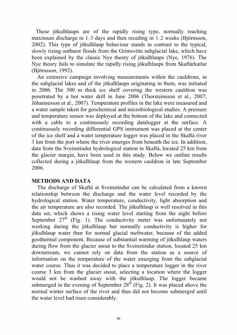
These jökulhlaups are of the rapidly rising type, normally reaching maximum discharge in 1−3 days and then receding in 1−2 weeks (Björnsson, 2002). This type of jökulhlaup behaviour stands in contrast to the typical, slowly rising outburst floods from the Grímsvötn subglacial lake, which have been explained by the classic Nye theory of jökulhlaups (Nye, 1976). The Nye theory fails to simulate the rapidly rising jökulhlaups from Skaftárkatlar (Björnsson, 1992). An extensive campaign involving measurements within the cauldrons, in the subglacial lakes and of the jökulhlaups originating in them, was initiated in 2006. The 300 m thick ice shelf covering the western cauldron was penetrated by a hot water drill in June 2006 (Thorsteinsson et al., 2007; Jóhannesson et al., 2007). Temperature profiles in the lake were measured and a water sample taken for geochemical and microbiological studies. A pressure and temperature sensor was deployed at the bottom of the lake and connected with a cable to a continuously recording datalogger at the surface. A continuously recording differential GPS instrument was placed at the center of the ice shelf and a water temperature logger was placed in the Skaftá river 3 km from the port where the river emerges from beneath the ice. In addition, data from the Sveinstindur hydrological station in Skaftá, located 25 km from the glacier margin, have been used in this study. Below we outline results collected during a jökulhlaup from the western cauldron in late September 2006. METHODS AND DATA The discharge of Skaftá at Sveinstindur can be calculated from a known relationship between the discharge and the water level recorded by the hydrological station. Water temperature, conductivity, light absorption and the air temperature are also recorded. The jökulhlaup is well resolved in this data set, which shows a rising water level starting from the night before September 27th (Fig. 1). The conductivity meter was unfortunately not working during the jökulhlaup but normally conductivity is higher for jökulhlaup water then for normal glacial meltwater, because of the added geothermal component. Because of substantial warming of jökulhlaup waters during flow from the glacier snout to the Sveinstindur station, located 25 km downstream, we cannot rely on data from the station as a source of information on the temperature of the water emerging from the subglacial water course. Thus it was decided to place a temperature logger in the river course 3 km from the glacier snout, selecting a location where the logger would not be washed away with the jökulhlaup. The logger became submerged in the evening of September 28th (Fig. 2). It was placed above the normal winter surface of the river and thus did not become submerged until the water level had risen considerably.

95

Figure 1. Discharge measured at Sveinstindur during the jökulhlaup. Labels on the x-axis denote the beginning of the corresponding day.

Figure 2. Water temperature measured in Skaftá 3 km from the glacier snout. Measurements before the sharp drop on September 28th are air temperature measurements, as the temperature sensor did not become submerged in water until on the evening of the 28th of September.

96

The distance from the glacier snout to the gauge at Sveinstindur affects the timing and the shape of the flood wave at the gauge location. This causes problems in estimating the speed of the flood front under the glacier, total storage of water under the glacier and other characteristics of the subglacial flood wave. To overcome this problem the one-dimensional hydraulic model HEC-RAS was used to calculate the expected shape and timing of the jökulhlaup at the glacier snout (Fig. 3) (Jónsson, 2007). In addition to the jökulhlaup component, the discharge measured at Sveinstindur includes the normal glacial discharge component in Skaftá and tributary rivers. Here the Skaftá discharge is assumed to be constant at 55 m3/s and tributary rivers entering the western branch of Skaftá between the glacier snout and Sveinstindur are assumed to contribute 20 m3/s.

Figure 3. Discharge of flood water during the jökulhlaup. Discharge out of the cauldron is shown as a solid line, discharge at the glacier snout is shown as a broken line and discharge at Sveinstindur is shown as a dotted line. To monitor the water accumulation in the subglacial lake and outflow during the jökulhlaup a GPS instrument that records and stores position and elevation once per day was placed at the centre of the ice shelf covering the western cauldron. Data on the water level increase was also obtained from a pressure transducer deployed at the bottom of the lake, which sent data via cable to a recording station at the surface. The cable broke in mid-September

97

due to increasing strain in the ice shelf and thus no pressure data are available from the transducer during the jökulhlaup. Comparison of the two data sets indicated a good match between results from the GPS recorder and the pressure transducer until the cable broke and thus we may expect the GPS data to provide accurate information after that. A relationship between the volume of the subglacial lake and the elevation of the overlying ice shelf was derived from information about the shape of the cauldron when the lake is empty. This made it possible to convert the lowering of the ice shelf to outflow of flood water from the lake. The glacier bottom is expected to be reasonably smooth and the lake assumes the form of a half dome extending upwards from the glacier bed into the ice. Prior to a jökulhlaup, the water is kept sealed in the lake by a minimum in the water potential due to the surface depression formed by melting at the base (Björnsson, 2002). The cauldron will thus take the shape of an inverted lake when the lake is emptied. RESULTS The 2006 jökulhlaup was comparatively small for the western cauldron with a maximum discharge of 120 m3/s of the outburst water at Sveinstindur, 135 m3/s at the glacier snout and 150 m3/s outflow from the cauldron (Fig. 3). The total volume of the outburst water from the cauldron was 64·106 m3 (Fig. 4). The maximum subglacial water storage during the flood was estimated to be 38·106 m3 by comparing the cumulative outflow from the cauldron with the cumulative outflow at the glacier snout (Fig. 4). Comparison of the estimated variation of the volume of the subglacial water storage (Fig. 4) with the flood discharge at the glacier snout (Fig. 3) shows that both reached a maximum at about the same time, indicating as expected that the subglacial pathway is able to carry the largest discharge when its average cross sectional area is at max-imum. Comparison of the timing of the flood front at the glacier snout and the initiation of subsidence within the cauldron gives the travel time of the flood front under the ice cap. As the GPS recorder in the cauldron only records elevations once per day, the timing of the start of the subsidence has an uncertainty of 24 hours. The start of the subsidence is between 8:00 on the 24th and 8:00 on the 25th of September. Then there is also uncertainty in the exact timing of the start of the jökulhlaup at the glacier snout, mainly because the daily discharge fluctuation masks the slow discharge increase in the beginning. The jökulhlaup can be assumed to start at the glacier snout between 13:00 and 22:00 on September 26th and thus the travel time of the subglacial flood wave from the cauldron to the snout was between 29 to 60 hours. The travel distance of the jökulhlaup, measured on a watercourse map drawn by Magnússon (2003), is 39 km and thus the mean travel speed of the

98

front of the flood wave between the cauldron and the snout was in the range 0.2−0.4 m/s.

Figure 4. Volume of floodwater. Water volume in the subglacial lake shown as a solid line, cumulative volume at the glacier snout shown as a broken line and volume stored subglacially is shown as a dotted line. At the location near the glacier snout, the temperature of the jökulhlaup water was between 0.0°C and 0.5°C (Fig. 2). The air temperature recorded at Sveinstindur varied between −1°C and 10°C during the jökulhlaup, but was between 2°C and 6°C most of the time. Hence, some warming of the outburst water may be assumed to take place on the 3 km long distance between glacier snout and the measuring point. In the morning of October 1st and during the nights of October 6th and 7th water temperatures are close to zero and the air temperature at Sveinstindur is also close to zero at the same time, so warming is probably minimal. Taken together, these measurement results indicate that the outburst water is at – or very close to – the freezing point as it emerges from beneath the ice cap. The temperature of the water in the cauldron was measured over a three month period before the jökulhlaup and found to be near 4°C (Jóhannesson et al., 2007) indicating that most of the thermal energy in the lake water was used for melting of ice on the way down the subglacial water course.

99

DISCUSSION A jökulhlaup from the Western Skaftá cauldron in late September and early October 2006 was monitored with simultaneous measurements within the cauldron and in the Skaftá river carrying the jökulhlaup. These measurements make it possible to describe the variation of outflow of flood water from the cauldron and the discharge of the flood at the glacier snout and thereby time-dependent variations in the storage of water in the subglacial water course. Measurements of the temperature of floodwater near the glacier snout, furthermore, show that the water emerges from the glacier near the freezing point. In this paper, we have presented some of the data along with a preliminary interpretation, but hopefully further modelling efforts using the data will contribute to an increased understanding of the mechanisms of fast rising jökulhlaups. The travel speed of the flood front under the glacier (0.2−0.4 m/s) is slow compared to the travel speed of subglacial water under normal conditions and flood waves in open channels. There are indications that the travel speed of the water increases at later stages for jökulhlaups in Skaftá, as exemplified by data collected after discharge had peaked during the 2002 jökulhlaup from the Eastern Skaftá cauldron. For this estimation we used data on: i) earthquake tremors indicating boiling or a minor volcanic eruption at the cauldron floor because of the pressure release accompanying the jökulhlaup, and ii) the concentration of suspended material in the jökulhlaup waters collected at the gauging station, which display a peak believed to result from the same boiling/eruption event. In this case, the flow speed under the glacier was estimated to be approximately 0.8 m/s. Outburst water is expected to be at or very close to the freezing point as it emerges from the glacier as thermal transport from jökulhlaup water to the surrounding ice walls in the tunnel is expected to be effective (Jóhannesson, 2002). The measured data provide support for this interpretation, but future studies should aim for water temperature measurements at the point of emergence at the glacier snout, to avoid the effects of warmer air on the river temperature. ACKNOWLEDGMENTS The Skaftárkatlar research project is funded and supported by The Icelandic Centre For Research (RANNÍS), Kvískerjasjóður, The NASA Astrobiology Institute, The National Power Company (Landsvirkjun), The National Energy Authority (Orkustofnun), The Hydrological Service Division (Vatnamælingar), The Public Roads Administration (Vegagerðin), the Icelandic Meteorological Office (Veðurstofan) and the Iceland Glaciological Society (Jöklarannsóknafélagið).

100

REFERENCES Björnsson, H. 1992. Jökulhlaups in Iceland: prediction, characteristics and

simulation. Annals of Glaciology, 16, 95−106 Björnsson, H. 2002. Subglacial lakes and jökulhlaups in Iceland. Global and

Planetary Change, 35, 255−271 Jóhannesson, T. 2002. Propagation of a subglacial flood wave during the

initiation of a jökulhlaup. Hydrological Sciences Journal, 47 (3), 417−434 Jóhannesson, T., Thorsteinsson, Th., Stefánsson, A., Gaidos, E., Einarsson,

B., Circulation and thermodynamics in a subglacial geothermal lake under the Western Skaftá cauldron of the Vatnajökull ice cap, Iceland. Geophysical Research Letters, VOL. 34, L19502, doi:10.1029/2007GL030686

Jónsson, S. 2007. Flóðrakning með takmörkuðum gögnum. M.Sc. thesis, University of Iceland, 92 pp. [In Icelandic]

Magnússon, E. 2003. Airborne SAR data from S-Iceland: analyses, DEM improvements and glaciological application, M.Sc. thesis, University of Iceland, 158 pp

Nye, J. F. 1976. Water flow in glaciers: Jökulhlaups, tunnels and veins. Journal of Glaciology, 17 (76), 181−207

Thorsteinsson, T., Elefsen, S. Ó., Gaidos, E., Lanoil, B., Jóhannesson, T., Kjartansson, V., Marteinsson, V. Th., Stefánsson, A., Thorsteinsson, Th. 2007. A hot water drill with built-in sterilization: Design, testing and performance. Jökull, 57, 71−82

Zóphóníasson, S. 2002. Rennsli í Skaftárhlaupum 1955−2002. SZ-2002/01, National Energy Authority, Hydrological Service, 16 pp. [In Icelandic]

101

HYDROLOGIC MODELING OF TWO CANADIAN WATERSHEDS USING THE NORTH AMERICAN REGIONAL

REANALYSIS DATA

Peter F. Rasmussen, Sung Joon Kim and Woonsup Choi

Department of Civil Engineering, University of Manitoba, Winnipeg MB, Canada R3T 5V6. E-mail: rasmusse@cc.umanitoba.ca

ABSTRACT In part due to concerns about the impact of climate change, there has been an increased interest in hydrological modeling of watersheds in Canada. Most of Canada is sparsely populated and a recurrent problem in hydrologic modeling is the lack of reliable weather data at the sites of interest. This paper explores the use of a recently released reanalysis data set for hydrologic modeling. The North American Regional Reanalysis provides temperature and precipitation on a 32 km by 32 km grid which is appropriate for hydrologic modeling. These data are used as input to the hydrological model SLURP in lieu of weather station data. For the particular cases considered here, it is found that model calibration using NARR data is quite acceptable and comparable to what can be obtained using interpolated weather station data.

INTRODUCTION Canada possesses a large proportion of the world’s freshwater stock. The management of this resource in the context of possible climate change is a significant challenge, not least because of the scarcity of streamflow and weather data in the remote regions of the country. Climate change impact assessment of water resources usually involves the use of a hydrologic model. However, the lack of data makes it difficult to develop reliable models. Often information must be interpolated from weather stations located far outside the basin of interest, a procedure which may result in poor model performance.

As an alternative to weather station data, one could consider data from reanalyses. Reanalysis data are obtained by running numerical weather prediction models that assimilate observations of variables such as surface pressure, relative humidity, precipitation, and temperature observed at different locations. The output of the reanalysis includes information about surface precipitation and temperature on a regular grid. These variables are the main input to most hydrologic models.

102

The objective of the present study is to compare calibrations of the hydrologic model SLURP with observed weather data and with data from the recently released North American Regional Reanalysis (NARR) data set. Two watersheds in the Winnipeg River basin in northern Ontario are modeled.

NORTH AMERICAN REGIONAL REANALYSIS (NARR) The North American Regional Reanalysis (NARR) is a reprocessing of historical meteorological observations using NCEP’s regional Eta model and various data assimilation systems. NARR’s spatial domain covers United States, Canada, and Mexico, and data from 1979 – updated in near real-time – are available at high temporal (3 hours) and spatial (32 km × 32 km) resolution. One key feature of this data set is the improved assimilation of observed precipitation (Mesinger et al., 2006) which makes it superior to previous global reanalysis data sets from NCEP-NCAR (Kalnay et al., 1996) and NCEP–Department of Energy (Kanamitsu et al., 2002). While NARR climatologies have been studied in some detail, the data set has rarely been used at daily time scales for hydrological modeling. Woo and Thorne (2006) applied SLURP to the Liard basin in the mountainous region of western Canada using climate data from various sources including weather stations, NCEP-NCAR Reanalysis, and NARR. They obtained similar model performance at the basin outlet but summer peaks were poorly simulated. Although their work provides valuable information regarding the utility of the NARR data set, it is limited to a specific region and was based on a short period of analysis.

STUDY AREA Two catchments were selected for this study: the Sturgeon River and the Troutlake River, located in the greater Winnipeg River basin in north-western Ontario, see Figure 1 and Table 1. Troutlake River and Sturgeon River gauging stations are located within 50 km from the Redlake Airport weather station and the Sioux Lookout Airport weather station, respectively. The basins are unregulated, but the runoff regime is influenced by many small lakes.

Table 1. Streamflow gauges in the study area.

Name Period of Record

Drainage Area

Sturgeon River at McDougall Mill 1961-2005 4450 km2 Troutlake River above Big Fall 1970-2005 2370 km2

103

THE SLURP MODEL The SLURP (“Semi-distributed Land Use-based Runoff Processes”) model (Kite, 1995) is a basin model which simulates runoff based on daily weather input (precipitation, mean temperature, relative humidity, and bright sunshine hours) and physiographic data (land cover and elevation). It is a semi-distributed conceptual hydrological model that was initially developed for modeling meso-scale Canadian watersheds as an alternative to the use of larger and more complicated hydrological models (Kite, 1995). This model is known to be robust and suitable for the northern environment at various geographical scales (Leenders and Woo, 2002). The model can be used to examine the effects

 

Figure 1. Location of river basins, weather stations, and NARR grid points (squared points are selected NARR grid points used for model input). that external factors such as climate change or changing land cover might have on the hydrologic cycle.

The model divides a basin into a number of "aggregated simulation areas" (ASAs). An ASA contains certain types of land cover and the vertical water balance is calculated for each land cover in each ASA. The water is routed to the outlet of each ASA and then to the outlet of the basin. SLURP simulates the vertical water balance with four storage tanks in each land cover in each ASA: canopy store, snow store, fast store, and slow store. Precipitation is provided as input of water to ASAs, and fluxes such as interception, sublimation, evapotranspiration (ET), surface runoff, interflow, and base flow are calculated from the storage tanks.

104

COMPARISON OF OBSERVED WEATHER DATA AND NARR DATA Data from the two weather stations (Redlake A, Sioux Lookout A) were used to calculate monthly climatologies of precipitation and temperature. These were compared to the corresponding NARR climatologies at the nearest grid points to provide an initial assessment of the suitability of NARR data for hydrological modeling. NARR mean precipitation from early summer through fall is lower than the observed, while NARR mean temperature is higher (Figure 2). With a few exceptions, the biases are relatively small, and one should keep in mind that weather stations may be influenced by localized effects.

 Figure 2. Mean monthly precipitation and temperature from weather stations and NARR.

RESULTS

SLURP calibration and validation using observed data The SLURP model was set up for each basin using digital land cover and elevation data. The digital elevation data were obtained from the NASA Shuttle Radar Topography Mission (SRTM), and land cover data sets were derived from the Advanced Very High Resolution Radiometer (AVHRR). Daily meteorological variables measured at the weather stations were used as input to each model.

J F M A M J J A S O N D0

1

2

3

4Sturgeon

Pre

cipi

tatio

n [m

m/d

ay]

J F M A M J J A S O N D0

1

2

3

4Troutlake

Pre

cipi

tatio

n [m

m/d

ay]

J F M A M J J A S O N D-20

-10

0

10

20

30Sturgeon

Tem

pera

ture

[°C

]

ObservedNARR

J F M A M J J A S O N D-20

-10

0

10

20

30Troutlake

Tem

pera

ture

[°C

]

105

The models were calibrated using streamflow data measured at the outlet of each watershed. Both weather stations have missing data, so calibration and validation were conducted using the most complete periods of record. The Sturgeon-model was calibrated for the period 1992-1995 and validated over the period 2000-2004. The Troutlake-model was calibrated for the period 1994-1997 and validated over 2000-2004. The key parameters adjusted during the calibration included maximum infiltration rate, retention constant for fast store, maximum capacity of fast store, retention constant for slow store, maximum capacity of slow store, rain/snow division temperature, canopy capacity, albedo, snowmelt rate, and evaporation-related parameters such as wilting point and field capacity. The calibration criteria included deviation of volume (Dv) of mean runoff and the Nash-Sutcliff Efficiency (E) of the daily runoff series.

Table 2 presents a summary of model performance statistics for the validation period. The results from the Sturgeon-model and the Troutlake-model are reasonable both in terms of volumetric error and goodness-of-fit.

Table 2. SLURP model performance using observed data for each basin (Validation).

Sturgeon Troutlake Observed mean runoff (m3/s) 46.13 20.68 Simulated mean runoff (m3/s) 49.14 19.86 Dv of mean runoff (%) 6.51 -3.96 E of daily runoff series 0.77 0.65

SLURP calibration and validation using NARR data Since the NARR data do not contain any missing data, the calibration and validation periods using NARR input data can be chosen arbitrarily. However, for the purpose of comparison with observed input data, the validation period was chosen to coincide with the same period considered in the previous section. The NARR-based models were calibrated using the years 1989-2000 and validated over 2000-2004. As shown in Table 3, the simulation statistics using NARR data are quite similar to the results obtained with observed data (Table 2).

Table 3. The SLURP model performance using NARR data for each basin (Validation).

Sturgeon Troutlake Observed mean runoff (m3/s) 46.14 20.68 Simulated mean runoff (m3/s) 45.04 19.86 Dv of mean runoff (%) -2.38 -3.99 E of daily runoff series 0.64 0.61

106

Daily streamflow simulation The quality of NARR simulated streamflow can be compared at different time scales. Climate change studies typically focus on longer time scales such as monthly or annual, with the possible exception of the study of extreme events such as floods. In this study, we considered daily, monthly, and annual flows.

Daily streamflow were simulated for each basin using NARR input for the period 1981-2004. The SLURP models calibrated with NARR were used. The simulated flows for the two watersheds are shown in Figure 3. There is a reasonable agreement between simulated and observed flows, although many

1981 1983 1985 1987 1989 1991 1993 1995 1997 1999 2001 2003 20040

50

100

150

200

250

300

Stre

amflo

w [m

3 /s]

Daily runoff simulation using NARR data at Sturgeon River

ObservedSimulatedPrecipitation (mm)

1981 1983 1985 1987 1989 1991 1993 1995 1997 1999 2001 2003 20040

50

100

Stre

amflo

w [m

3 /s]

Daily runoff simulation using NARR data at Troutlake River

ObservedSimulatedPrecipitation (mm)

 

Figure 3. Daily streamflow simulation. Top: Sturgeon River. Bottom: Troutlake River.

peak flows, especially in the spring, are underestimated in the simulations. One can speculate whether the inability to adequately simulate peak flows is related to the hydrologic model or the NARR input data or a combination of the two. The climatologies shown in Figure 2 suggest that NARR has a negative precipitation bias at the Sturgeon basin (Red Lake Airport) in the month of June where much of the spring runoff takes place. On the other hand, peaks appear to be underestimated also in the case where flows are simulated with observed weather information (figures not shown). It seems reasonable to assume that the inability to reproduce many of the observed peak flows is related more to the hydrologic model than to the input data.

107

Monthly runoff Observed and simulated daily flows were aggregated to monthly flows and examined in more detail. The mean monthly flows provide some insight into seasonal biases. Figure 4 shows a plot of the means of recorded monthly flows, flows simulated with observed data, and flows simulated with NARR data. For Sturgeon River, there is relatively little difference between the two set of simulated flows. Both sets of simulations underestimate mean monthly flows in May and June, a consequence of the underestimated spring peak flows seen in

J F M A M J J A S O N D0

10

20

30

40

50Sturgeon

Dis

char

ge [m

3 /s]

J F M A M J J A S O N D0

10

20

30

40Troutlake

Dis

char

ge [m

3 /s]

 Figure 4. Mean monthly streamflow record and simulated runoff with different input data sets (observed data and NARR data).

the daily flows. The negative biases in May and June combined with the calibration criterion of minimizing the overall volumetric error leads to some overestimation in other months.

For Troutlake River, the performance of the two simulation sets in terms of monthly means is also quite similar. The underestimation of flows in May and June are somewhat smaller than for Sturgeon River.

Figure 5 shows time series of observed and simulated monthly mean runoff. Some of the problems with the simulated daily streamflows are also present in the monthly streamflows. In particular, there appears to be a tendency that months with high runoff are underestimated and months with low runoff are overestimated. Further fine-tuning of model parameters could possible reduce this problem.

108

Annual discharge In the final comparison, daily flows are aggregated to annual flows to assess if the inter-annual variability of flows can be properly simulated using NARR data. The results are shown is Figure 6. For the years where reasonably complete observed weather records are available, the corresponding simulated flows are also shown. The NARR simulated flows appear to be more inaccurate than flows simulated with observed weather data. While the general variation is

1981 1983 1985 1987 1989 1991 1993 1995 1997 1999 2001 2003 20040

50

100

150

200

Stre

amflo

w [m

3 /s]

Monthly Mean Runoff at Sturgeon River

Observed RunoffSimulated Runoff

1981 1983 1985 1987 1989 1991 1993 1995 1997 1999 2001 2003 20040

10

20

30

40

50

60

Stre

amflo

w [m

3 /s]

Monthly Mean Runoff at Troutlake River

Observed RunoffSimulated Runoff

Figure 5. Observed and simulated monthly runoff series. Top: Sturgeon River. Bottom: Troutlake River.

reasonably preserved by the NARR simulation, some years are clearly not well represented.

Table 4 summarizes goodness-of-fit statistics for NARR simulated flows in the two basins, considering the different levels of aggregation.

Table 4. Model performance for different levels of aggregation. Period is 1981 to 2004.

Daily Monthly Annual Mean Monthly

Sturgeon River E 0.62 0.66 0.60 0.89 Dv 0.78 0.82 0.80 0.78

Troutlake River E 0.48 0.51 0.39 0.57 Dv 16.0 15.9 16.0 16.0

109

1980 1985 1990 1995 2000 20050

200

400

600

800

1000Sturgeon

Dep

th [m

m]

1980 1985 1990 1995 2000 20050

200

400

600

800

1000Troutlake

Dep

th [m

m]

Year

PQ RecordQ NARR SimQ Obs Sim

 Figure 6. Annual runoff simulation for Sturgeon and Troutlake.

CONCLUSIONS Good quality weather data are always desirable in the calibration of and simulation with hydrologic models. When representative weather data are available from weather stations in the watershed, these will in most cases be preferable. However, when precipitation information must be interpolated from weather stations located far from the basin, as is typically the case in data sparse regions, there is likelihood that weather input variables will be misrepresented. For such cases, the use of high-resolution reanalysis data may be a viable alternative. Our investigation of two watersheds in the Winnipeg River basin suggests that in a number of aspects streamflow simulated with weather information from the North American Regional Reanalysis are comparable to streamflow simulated with observed weather data. Daily and monthly data were found quite acceptable, but the representation of interannual variability was found somewhat deficient. This is an ongoing research project and future efforts will include applications to other sites as it is difficult to draw general conclusions from only two applications.

110

ACKNOWLEDGEMENT The research report here is funded by Manitoba Hydro and by the Natural Sciences and Engineering Research Council of Canada. REFERENCES Kalnay, E., Kanamitsu, M., Kistler, R., Collins, W., Deaven, D., Gandin, L.,

Iredell, M., Saha, S., White, G., Woollen, J., Zhu, Y., Chelliah, M., Ebisuzaki, W., Higgins, W., Janowiak, J., Mo, K. C., Ropelewski, C., Wang, J., Leetmaa, A., Reynolds, R., Jenne, R. and Joseph, D. 1996. The NCEP/NCAR 40-Year Reanalysis Project. Bulletin of the American Meteorological Society, 77: 437-471

Kanamitsu, M., Ebisuzaki, W., Woollen, J., Yang, S.-K., Hnilo, J. J., Fiorino, M. and Potter, G. L. 2002. NCEP–DOE AMIP-II reanalysis (R-2). Bulletin of the American Meteorological Society, 83: 1631-1643

Kite, G. W., 1995. The SLURP Model, in Computer Models of Watershed Hydrology, edited by V. P. Singh, chap. 15, pp. 521- 562, Water Resources Publications

Leenders, E. E., and M. Woo, 2002. Modeling a two-layer flow system at the subarctic, subalpine tree line during snowmelt. Water Resources Research, 38, 1202, doi:10.1029/2001WR000, 375

Mesinger, F., DiMego, G., Kalnay, E., Mitchell, K., Shafran, P. C., Ebisuzaki, W., Jović, D., Woollen, J., Rogers, E., Berbery, E. H., Ek, M. B., Fan, Y., Grumbine, R., Higgins, W., Li, H., Lin, Y., Manikin, G., Parrish, D. and Shi, W. 2006. North American Regional Reanalysis. Bulletin of the American Meteorological Society, 87(3): 343-360

Woo, M.-k. and Thorne, R. 2006. Snowmelt contribution to discharge from a large mountainous catchment in subarctic Canada. Hydrological Processes, 20: 2129-2139

111

RADIATION BUDGET IN A SNOW-COVERED SUBALPINE FOREST AND ITS INTERACTIONS WITH THE SNOWPACK

Tobias Jonas1, Manfred Stähli2, David Gustafsson3

1WSL, Swiss Federal Institute for Snow and Avalanche Research SLF,

Davos, Switzerland, 2Swiss Federal Institute for Forest, Snow and Landscape Research WSL, Birmensdorf, Switzerland, 3Royal Institute of

Technology KTH, Stockholm, Sweden

ABSTRACT Boreal and subalpine forests cover large areas of the Northern Hemisphere land surface. Seasonal snow is strongly influence by the presence of a forest canopy. Changes in the radiation budget and of turbulent transport processes modify accumulation and ablation of the snowpack and subsequent runoff processes. In this study we concentrate on interactions between the snowpack and the radiation budget inside the forest. Short-wave and long-wave radiation inside forests are highly variable in space and time due to the heterogeneity of the canopy. In winter the interception of snow in trees and a non-uniform accumulation of snow on the ground lead to an even more complex radiation dynamics. Therefore, representative measurements of net radiation, albedo and transmissivity inside a snow-covered forest require an elaborate set-up. In this study we present observational data of the radiation budget inside a coniferous subalpine forest covering four winter seasons using a novel measuring set-up. A four-component net-radiometer was mounted on a carriage and constantly moved back and forth on a 10-m rail. The device thus captured the natural variability of the net-radiation and of the forest floor albedo, respectively. Further radiation measurements above and outside the forest as well as complementary snow measurements (depth and water equivalent) enabled analysing the reciprocal effects of the radiation budget on the snowpack and vice versa.

112

ICE AND WEATHER CONDITIONS IN THE GULF OF RIGA, THEIR IMPACT ON RIGA HARBOR WINTER NAVIGATION, 1996-2006

Inese Mikelsone 1, Élise Lépy 2 and Yuriy Shishkin 3

1 National Board of Fisheries, Republikas square 2, Riga, LV- 1010, Latvia, e-mail: inese.mikelsone@gmail.com

2 PhD Student, Laboratory GEOPHEN UMR LETG 6554 CNRS, University of Caen, Esplanade de la Paix, 14032 Caen Cedex, France, e-mail:

elise.lepy@unicaen.fr 3 Latvian Environment, geology and meteorology agency, Maskavas Street 165,

Riga, LV-1019, Latvia, e-mail: jurijs.siskins@lvgma.gov.lv

ABSTRACT Sea ice is very important hydrological element of the Baltic Sea

environment, directly or indirectly affecting many of the oceanographic, climatic, ecological, economical and human parameters that characterize the region. Winter navigation requires an icebreaker’s assistance to provide safe and effective navigation in ice in the Gulf of Riga. Analysis of maximum ice extent in the Baltic Sea within 1901-2006 period shows continued tendency to decrease, however several winters with quite severe ice conditions for navigation were observed in period 1996-2006.

INTRODUCTION

The Baltic Sea is partly covered with ice every winter, mainly the Gulfs of Bothnia, Finland and Riga. The maximum annual ice extent is between January and March, when ice covers 52,000-420,000 km² and on average 218,000 km² (Lindqvist and Gullne, 2006). The Gulf of Riga freezes almost every 4 years (Pastors et all, 1996).

In winter period in the Gulf of Riga, fast and drift ice can be observed. Fast ice exists in coastal areas but drift ice has dynamic nature being forced by winds and currents. Ridges and brash ice are most significant obstructions to navigation (Pastors et all, 1996).

Winter navigation requires icebreaker (for the Gulf of Riga – “Varma”) assistance to provide safe and effective navigation in ice. It is very important also for gulf’s ports work.

113

ICE CONDITIONS IN THE GULF OF RIGA Ice formation in the Gulf of Riga starts in the Bay of Pärnu where new ice

forms in mid-December (Fig. 1).

Figure 1. The ice formation dates (I. Mikelsone), a) early; b) average.

In February, intensive ice formation and freezing can be observed in the

whole gulf. In severe winters, the gulf is entirely covered with ice in January. In very mild winters, the gulf does not freeze at all (Pastors et all, 1996).

The formation of fast ice usually begins at the coast, and further extends in parallel with isobaths. Maximum development of the fast ice falls on the end of February – beginning of March (Wang et all, 2003).

Some pictures of the ice cover in the gulf were taken in ice observing flight on 30 March, 2005 (Fig. 2 and Fig. 3).

Figure 2. Central part of the Gulf of Riga (E. Lépy).

Figure 3. Irbe straight (E. Lépy).

114

Ice processes can be described according to 7 distinguished zones of freezing probability (Fig. 4).

Figure 4. Freezing probability (%), of the gulf’s zones (I. Mikelsone).

Winter classification in Latvia was created regarding the sum of negative daily mean air temperatures: severe, average and mild. This sum characterizes the severity of ice season in the Gulf of Riga: 330 °C corresponds to average winters; up to 670 °C the winters are severe; and below to 330 °C, it is mild (Kostjukov, 2002). This classification can show some regional differences in Latvia - in the period 1996-2006 (data were obtained from Latvian Environment, geology and meteorology agency), station Rīga (southern part of the gulf) has known 5 average and 5 mild winters, station Kolka (western part of the gulf) 2 average and 8 mild winters, whereas station Ainaži (eastern part of the gulf) has known 1 severe, 5 average and 4 mild winters (Tab. 1).

Table 1. Sum of negative temperatures, °C.

YEAR STATION NAME

RĪGA KOLKA AINAŽI 1996/1997 -341 -180 -339 1997/1998 -255 -141 -287 1998/1999 -499 -270 -487 1999/2000 -183 -85 -183 2000/2001 -224 -166 -269 2001/2002 -271 -157 -313 2002/2003 -584 -458 -707 2003/2004 -307 -215 -351 2004/2005 -391 -153 -480 2005/2006 -582 -407 -605

115

Different approach for classification of winters was developing in Finland – 5 winter classes according to the maximum ice extent in the Baltic Sea (Tab. 2).

Table 2. The Baltic Sea winters classification (Leppäranta and Omstedt, 1999).

Winter class Maximum ice extent, thousand km² Maximum ice extent, %

Very mild to 81 to 19 Mild from 84 to 139 from 20 to 33 Average from 148 to 272 from 35 to 65 Severe from 280 to 382 from 67 to 91 Very severe from 390 to 420 from 93 to 100 In the last decade, in the Baltic Sea region regarding to the maximum of ice extent, has been observed 5 average (Fig. 5) and 5 mild winters (Linqvist et all, 2006). This classification shows close connection with previous classification method for the Gulf of Riga.

050

100150200250300350400450

1997

1998

1999

2000

2001

2002

2003

2004

2005

2006

thous.km2

Very severe

Severe

Average

Mild

Very mild

Figure 5. Maximum ice extent and winter types in the Baltic Sea, 1996-2006.

Analysis of maximum ice extent within 1901-2006 period shows continued

tendency to decrease (Fig.6), however several winters with quite severe ice conditions for navigation were observed in 1996-2006.

116

y = -0.1449x + 193.72

0

50

100

150

200

250

300

350

400

45019

01

1907

1913

1919

1925

1931

1937

1943

1949

1955

1961

1967

1973

1979

1985

1991

1997

2003

thou

s.km

2

Figure 6. Maximum ice extent in the Baltic Sea and tendencies, 1901-2006

CARGO TURNOVER IN PORTS OF THE GULF OF RIGA

Riga harbor and six small ports (Skulte, Mersrags, Salacgriva, Roja, Lielupe and Engure) are located in the Gulf of Riga. Their main aspects are:

o The Baltic Sea transport; o Fishing ships basing place; o Yacht tourism.

Analyzing dynamic of cargo turnover (1996-2006) in Riga harbor and in small ports (data were obtained from Central Statistical Bureau), trend shows strong increasing tendency (Fig.7). Export dominates in the cargo turnover structure.

If the Gulf of Riga in winter period has difficult ice conditions large numbers of ships were turned to the other Baltic Sea ports where shipping conditions were better and it has some impact on Riga’s harbor cargo turnover in winter period. Especially negative impacts from difficult ice conditions in the Gulf of Riga have small ports. They can be closed because the small ports fairways are too shallow for icebreaker “Varma”.

117

0.0 5000.0 10000.0 15000.0 20000.0 25000.0

19951996199719981999200020012002200320042005

thous. tons

Small portsRiga harbor

Figure 7. Cargo turnover in Riga harbor and small ports, 1995-2006. NUMBER OF INCOMING SHIPS TO RIGA’S HARBOR

Navigation to Riga’s harbor and small ports can be difficult in the Gulf of Riga even in average winters ice conditions. Navigation to small ports can stop for several days – it depends on severity of winter and availability of icebreaker.

To analyze ice and meteorological parameters impact on winter’s navigation 1996-2006, large number of incoming ships to Riga’s harbor (Fig.8) was used (data were obtained from Maritime Administration of Latvia).

Figure 8. Number of incoming ships to Riga harbor and sum of negative temperatures in Riga in winters 1996-2006.

-600.0

-500.0

-400.0

-300.0

-200.0

-100.0

0.0

1996

/199

7

1997

/199

8

1998

/199

9

1999

/200

0

2000

/200

1

2001

/200

2

2002

/200

3

2003

/200

4

2004

/200

5

2005

/200

6

tem

pera

ture

sum

, 0 C

1200

1300

1400

1500

1600

1700

1800

1900

2000

inco

min

g sh

ips

Temperature Ships

118

SOME METEOROLOGICAL PARAMETERS IMPACT ON WINTER NAVIGATION

Wind regime has some impacts on ice conditions especially in coastal areas. Different wind directions in the gulf can make feasible navigation or some of them can cause ice ridging and compacting. Wind directions for different parts of gulf can definite as “good”- ice drift direction from coast, “not good” – ice direction to coast and “neutral” – ice drift along coast (Tab.3).

Table 3. Wind probability (%). Good (+), not good (-), neutral (0) directions (Pastors et al, 1996).

Station NOV-DEC JAN-FEB MAR-APR + - 0 + - 0 + - 0

Rīga 66 15 19 58 23 19 51 35 14 Ainaži 49 29 22 44 27 29 25 51 24 Kolka 20 55 25 26 49 25 24 53 23

Data from this table can be used in planning winter navigation for choosing

possible fairway in ice. Snow in beginning of ice formatting process haste water cooling and ice

formatting. After starting ice process formation snow cover not only decelerates ice thickness increasing but also makes addition resistance for navigation. Snow depth maximum on ice usually observe in March – about 15 cm (Pastors et all, 1996). CONCLUSION

All collected and estimated data are used to understand ice and weather conditions impact on very important sector of economy and give a small look on ice conditions tendency in short time scale.

Ice and weather conditions have significant impact on winter navigation in the Gulf of Riga especially in average and severe winters when icebreaker “Varma” can not provide effective assistance in the gulf’s fairways.

In winters 1996-2006 close connection are shown between maximum of ice extent in the Baltic Sea and sum of negative temperatures in the Gulf of Riga.

In the Gulf of Riga winter severity can be different for its’ regions: milder in southern and western parts and severe in eastern part. This regional ice and weather condition differences also has a big impact on ports’ works.

Analyzing different meteorological parameters for period 1996-2006 was estimated, that in the gulf much more days with ice were observed in March but ice processes started later.

119

REFERENCES Kostjukov J. 2002. Ice conditions in the Gulf of Riga// Proceedings of the Third

Workshop on the Baltic Sea Ice Climate. October 5-8, 1999, Stawiska, Poland. – Warszawa: The Institute of Meteorology and Water Management, - 53-55

Leppäranta M., Omstedt A. 1999. A Review of Ice Time series of the Baltic Sea// Publications of Second Workshop on the Baltic Sea Ice Climate. - University of Tartu: Department of Geography, – 7-12

Lindqvist J., Gullne U. 2006. A Summary of the Ice season and icebreaking activities 2005/2006. – Sweden: Swedish Meteorological and Hydrological Institute, - 53 pp

Pastors A., Glazaceva L., Kostjukovs J., Zaharcenko E. 1996. The Gulf of Riga. – Riga: State Hydrometeorological agency, – 418 pp (in Russian)

Wang K., Leppäranta M., Köuts T. 2003. Natural process of sea ice evolution in the Gulf of Riga. Fourth Workshop on the Baltic Sea Ice Climate. Norrköping, Sweden 22-24 May, 2002// SMHI Oceanografi No. 72, 2003. – Göteborg: SMHI, - 77 – 77

120

TOWARDS INTEGRATED SYSTEMS FOR ARCTIC HYDROLOGY – APPLICATIONS AT

THE FINNISH HYDROLOGICAL SERVICE

Markku Puupponen, Finnish Environment Institute, P.O.Box 140, FI-00251 Helsinki, Finland, e-mail: markku.puupponen@ymparisto.fi

ABSTRACT The Arctic-HYDRA programme is a large umbrella for hydrological re-search in the Arctic. As a multidisciplinary effort, it links hydrology with many other fields of science in geophysical, environmental and social sec-tors. The spatial focus is the Arctic Ocean drainage basin, but climate and land-atmosphere processes connect Arctic-HYDRA with global studies. From the temporal point of view, the first phases of the programme are forming an IPY (International Polar Year) component between 2007 and 2009. However, the goals of Arctic-HYDRA also aim at long term activi-ties beyond IPY. This multi dimensional activity calls for integration. There are numer-ous possibilities to gain synergy: between operational services, between disciplines, between regions, between data controlling systems – and be-tween any combinations of these four components. This paper will focus on the integrated hydrological system concept, where observations, proc-ess studies, models, and data systems are effectively linked to produce synergy benefits; this approach is also an important strategic goal of the Arctic-HYDRA. Some developments of the Finnish Hydrological Service have turned out to be successful steps towards integration, and they can offer perspectives to large scale and even Pan-Arctic applications. The Finnish Hydrological Service is located at the Finnish Environment Insti-tute (SYKE), which is both service and research oriented and strongly seeks for integrated solutions. As a National Hydrological Service, SYKE is operating systems for monitoring, modelling, data processing, and water related geo-information. All of these systems have national coverage and they are mu-tually integrated at several levels. The first three components – monitor-ing, modelling and data processing – are also integrated at daily opera-tional level. The Finnish national hydrological monitoring programme comprises some 1,200 observation sites, which are financed and maintained either by the hydrological service, other research community, or water industry. About 60% of the stations transfer almost real-time data, which means that these data are collected at a maximum frequency of one day.

121

Hydrological modelling is represented by the Watershed Simulation and Forecasting System (WSFS), which is highly operational and run daily or more frequently. The hydrological model is based on the HBV concept, and it has been further developed at SYKE since 1980s. WSFS makes surface or ground water forecasts for some 1,000 sites, and simu-lates the basic water balance components at some 6,000 sub catchments using daily time step. The system also generates hydrological maps, automatic flood and snow load warnings and many other products for wa-ter resources management, other expert services, and the public. The fore-casts and products of WSFS are available on the Internet. The processing of monitoring data is carried out by a set of data sys-tems. It is composed of a data collection and quality control software, three databases, and a software package for calculation and analyses. The software for data collection and control, and one database (data delivered by the Meteorological Institute) are used by the operator only. One data-base (for momentary values or separate measurements) and the software package for calculation and analyses are currently for internal use (within the whole Environmental Administration), and the main database is web based and will be released into the Internet use during 2008. Geo-information databases are currently being developed into more dy-namic data systems. The three components are for lakes (56,000 objects), rivers (25,000) and river basins (6,000). The above basic blocks of the integrated hydrological system interact at several level. The monitoring and data systems continuously transfer al-most real-time data into hydrological models, and if models diagnose some data as inconsistent, this feedback is communicated into the data and monitoring systems. Most ground observations are point measure-ments, while models produce areal values e.g. for precipitation, snow, evaporation and so on. As wide scale models also simulate run-off for high number of sub basins, in-situ measurements are not always needed. On the other hand, real-time observations at important sites keep the status of models correct. Satellite images on snow cover are used in the snow calculations of hydrological models. Good quality geo-information on water resources is essential basic information for hydrological models, and map interfaces have proved to be applicable, informative and user friendly. The list of examples could be continued. In addition to the operational components (observation, modelling and data systems), the integrated concept includes process studies. Process studies are made for various purposes, but two main objectives and cate-gories can be marked out. On one hand, large scale process studies aim at better modelling at a river basin scale. This work can be considered as model development, and to be successful, it should seek for balance be-tween relevant science aspects and simple, applicable solutions. On the

122

other hand, small scale process studies produce new information on hy-drological processes. During the project phase, large and small scale stud-ies are separate processes, but in the long run, they interact. Thus both categories of process studies are linked with operational modelling and furthermore with observation and data systems. The above discussion means that structures and contents of monitoring programmes should support both modelling and process studies, and vice versa, scientific knowledge should be used to minimise costs of measure-ment systems. Our experience shows that integration is cost effective – both from the point of view of system operation and scientific relevance. From the point of view of Arctic-HYDRA, the key question is how to develop national or regional systems into Pan-Arctic. To what extent can local systems be clustered – e.g. by means of internet and user interface? What activities require completely uniform solutions? Probably monitor-ing systems and process studies are the most independent components, which should be based on common objectives but can be operated on na-tional or corresponding bases. As data systems and related services pro-duce information out of data, they have an "integration" role and they should have an umbrella, a user interface to provide consistent services and products. Modelling will probably be composed of river basin, re-gional and global/Pan-Arctic models. The current models should probably be mapped and evaluated, and the scientific community should set targets fior Pan-Arctic hydrological models and their integration with atmos-pheric and Arctic Ocean models. From the hydrological point of view, one of the greatest challenges is to include adequate ground and river system description into large scale models.

123

PROCESSES AND MORPHOLOGIES OF ICELANDIC GULLIES AND IMPLICATIONS FOR MARS

Benjamin A. Black1 and Thorsteinn Thorsteinsson1

1Hydrological Service Division, National Energy Authority (Orkustofnun), Grensásvegur 9, 108 Reykjavík, Iceland; e-mail: bab13@hi.is, thor@os.is

ABSTRACT Iceland provides an excellent natural laboratory for studies of

debris flows and other steep slope water-related transport processes. These phenomena are important for the understanding of terrestrial landscape evolution. Basic morphological similarities between Icelandic gullies and controversial, potentially water-related gullies on Mars suggest that Icelandic gullies may also offer insight into the conditions and mechanisms of Martian gully formation. An understanding of how different processes lead to different morphologies in Iceland could identify diagnostic features to help fingerprint the range of processes operating on Mars. Aerial photographs of study sites in Iceland, along with on-site temperature sensors, provide information about the evolution of gully morphology and timescales of gully activity. We use our preliminary observations to investigate the roles of snowmelt, rainfall, and topography in shaping Icelandic steep-slope features.

INTRODUCTION Debris flows are water-mobilized gravity flows that carry a poorly mixed slurry of rock and sediment downslope. They are one of the major landforms that influence the shape of high-latitude slopes (Åkerman, 1978; Rapp, 1986), and they are ubiquitous in Iceland. Their distinctive signature morphology consists of a chute-like head alcove, a channel (often raised with levees), and a conical debris apron; taken together, these constitute a ‘gully’. Other steep-slope processes active in Iceland include snow avalanches, nivation, gelifluction, rockfall, and fluvial erosion. Many of these processes overlap spatially with debris flows, competing to shape the morphology of gullies. Previous studies of debris flows in Iceland (e.g. Decaulne and Sæmundsson, 2007) have focused on their natural hazard relevance. We intend to explore the geomorphologic roles of steep-slope processes in Iceland, and we will investigate the potential relevance of these terrestrial processes to gullies and gully-like forms on Mars.

124

In 2000, Malin and Edgett published images of alcoves, sinuous channels, and debris aprons photographed by the Mars Orbiter Camera (MOC). They championed these gullies as evidence of recent liquid water flowing across the surface of Mars. Substantial controversy ensued, as the planetary science community argued over how the gullies had formed and whether liquid water was involved. Three main end-member hypotheses emerged: liquid water from a subsurface aquifer (Malin and Edgett, 2000; Heldmann, 2007), runoff from melt of snow deposited during a high-obliquity period (Christensen, 2003; Dickson et al., 2007), and dry granular flow (Treiman, 2003). The pitch of the discussion was heightened with Malin et al.’s (2006) announcement of new, bright deposits in two gullies that had appeared since the last set of photographs was taken in 1999. In the absence of primary data on Martian gullies beyond orbital imagery and spectral analysis, terrestrial analogs have proven to be a valuable resource for testing new ideas about Martian gullies. Previous terrestrial analog studies include Costard et al.’s (2002) work on debris flows in Greenland, Hartmann et al.’s (2003) study of gullies in Iceland, and the work of Head et al. (2007) in the Antarctic Dry Valleys. With its easy accessibility, Iceland offers an excellent opportunity to study a broad range of steep-slope features and to test their viability as Martian analogs (Black and Thorsteinsson, 2008). Simple debris flows are the Icelandic landform most similar in appearance to the classic Martian gully. Debris flows require ample water, which is in limited supply on Mars, although liquid water runoff at the Martian surface is possible with the assistance of a plugged aquifer (Malin and Edgett, 2000; Heldmann et al., 2007) or a brine (Marchant and Head, 2007). But we stress the diversity of steep-slope processes in Iceland, many of which require little or no liquid water to activate. As Åkerman (1978) has pointed out, gully activity on Earth may have fluctuated since the end of the last glaciation. The basic gully structures may be several thousand years old (Rapp, 1987). However, as our results will show, many processes continue to substantially modify gully morphology in the present day. It is therefore important to identify and describe the full range of these ongoing erosional, transport, and depositional processes. An understanding of how different processes lead to different morphologies in Iceland could provide diagnostic features to help identify the range of processes operating on Mars. With these considerations in mind, the ultimate goals of our investigation are as follows:

• To gain an understanding of the mechanisms of gully formation and their relationship to gully appearance. The basic mechanisms driving debris flows in Iceland have been described by Decaulne and Sæmundsson (2007), and they include: rain on snow, snowmelt

125

induced by a rapid temperature increase (>10ºC in 24 hours), and long-lasting and/or intense rainfall. The morphological expression of these various causes, however, requires further study.

• To analyze gully activity over longer timescales. • To characterize the evolution of gully morphology.

METHODOLOGY We combine ongoing field measurements and observations with analysis of aerial photographs provided by Landmælingar Íslands (LMÍ). The field measurements include snow density, snow temperature, gully-bottom temperature, slope, and the basic dimensions of the gully. Gully-bottom temperatures are obtained with two electronic temperature sensors, one on Ármannsfell and one on the eastern part of the Esja massif. These Starmon-type sensors have an accuracy of ±0.05°C and they take a temperature reading every minute. We have installed them in the bottom of gully channels, in the hope that episodes of meltwater flow in the gullies will leave a temperature signature. We expect that any snowmelt events resulting in top-to-bottom flow should appear as periods of constant near freezing temperature. The goal of our field measurement program is to assemble a record of changes in gully activity and morphology over the course of a full year, thereby illuminating any seasonal dependence. The aerial photographs (e.g. Figure 2) promise additional insights into rates of gully formation, stages of activity and dysfunction, and areal distribution. They range in scale from roughly 1:20,000 to 1:60,000. Complete coverage of Iceland is available at intervals of roughly 10 years, from 1945 onwards. RESULTS Field Observations Substantial volumes of windblown snow accumulate in the alcoves and channels of Icelandic gullies. Excavation of a gully on Mt. Esja showed that snow depths at the top of the channel were greater than 2.5 meters, even when the adjacent slope was bare. Observation of other Icelandic gullies indicates that this degree of concentration is not unusual. Nivation (snow wash) and focused snow avalanches may be important geomorphic factors as a result (Rapp, 1986). Nivation over millennia may be a primary agent in shaping the scalloped alcoves where Icelandic gullies originate. Snow density and snow temperature profiles from gullies in Southwest Iceland show temperate spring snow packs, with snow responding to air temperature in the top few centimeters but stabilizing at or slightly below zero degrees Celsius throughout the remainder of the profile. Densities range from 0.26 kg/m3 to 0.554 kg/m3.

126

Icelandic gullies vary in cross-section from V-shaped to U-shaped channels. Luckman (1977) has observed that repeated, concentrated snow avalanches may produce U-shaped chutes, which cannot be easily explained by running water. Among the V-shaped channels, there is a wide spread in depth/width ratios. This may prove a fruitful area for additional measurement.

Figure 1. (Top): October temperature measurements from a sensor at Ármannsfell (elev. ~400 m) along with hourly precipitation (gray bars) and temperature at the nearby Þingvellir weather station.

Figure 1. (Bottom): An enlargement of a period of potential gully flow.

Unlike on Mars (Christensen, 2003), older, degraded, and inactive gullies are clearly present in Iceland. Previous authors have used lichen to estimate

127

the elapsed time since the most recent debris flow activity, finding recurrence intervals ranging from 40-500 years in north Sweden (Rapp, 1986). The temperature sensors reveal one potential episode of flow in the Ármannsfell gully on October 26-27, shown in Figure 1. The three days preceding October 26 were unusually warm, with heavy precipitation (Figure 1). Precipitation on the day preceding the anomaly was especially heavy. We infer that a combination of a warm air mass passing through the area and heavy rain may have triggered snowmelt in the alcove and channel, leading to runoff in the

Figure 2. The image at the top provides context of the ~6 km western face of Mt. Esja; the second row and third row present close-ups of fan morphology at two sites in 1945, 1968, 1977, 2000, and 2008. 2008 images are ground-based from January; all other images are aerial, and taken during the summer (courtesy of LMÍ). The gully sites in the second and third rows are indicated by the dashed and solid rectangles, respectively, in the context image. Note the decadal-scale changes in the main channels through the debris aprons, and the snow-filled channels in the 2008 images.

gully. However these results must be viewed with care, as a snow pack around the sensor could also cause zero temperature readings. The fact that there is rarely only one process at work, even in the same gully, has complicated our efforts to isolate cause and morphological effect. Orientation does not appear to have a strong effect on large-scale gully distribution in Iceland, although certain faces at specific sites host more

128

gullies than others. Similarly, geology is not a major control either: gullies are found both on hyaloclastic formations and layered basalts. Interestingly, gullies can also occur when there is no upslope drainage network, supporting the role of snow accumulation and melt as a primary driver of gully formation in some cases. Observations from Aerial Photographs Analysis of aerial photographs helped us to bracket the timescales of change in Icelandic gullies. On a decadal scale, changes in debris aprons and distal channels were plentiful. Over the course of 50 years, one small new debris flow track appeared on a ~6km face of Mt. Esja (Figure 2, top). We also identified a transient set of intriguing parallel incisions, which appeared and disappeared in tens of years. Clearly, Icelandic gullies are being actively modified on decadal timescales in the present day. But equally noticeable was the lack of major changes in the landscape of the slope. We did not identify any changes in alcove morphology, and the number of major gullies and channels remained static. We therefore suggest that primary development of gully morphologies occurs on much longer timescales than those for which aerial records are available. Figure 2 presents close-ups (from 1945, 1968, 1977, 2000, and 2008) of two adjacent sites on Mt. Esja. Changes in the channel paths through the debris aprons, and new debris deposits, are visible at both sites. Whipple and Dunne (1992) argue that debris fan morphology reveals flow rheology: debris-rich flows roughen fan surfaces, and flows with high sediment loads fill in channels, leading to avulsion and the creation of new depositional termini. Time-staggered aerial photographs like those in Figure 2 allow us to analyze the evolution of debris aprons. We observe that individual deposits tend to be rounded and lobate, but as individual deposits accumulate, leading to distal channel avulsion, the overall debris apron may become digitate. This process is illustrated in the bottom sequence of Figure 2. DISCUSSION Implications for Iceland Rapp (1960) and Åkerman (1978) have noted that present rates of talus formation in Spitsbergen seem too low to be consistent with the observed debris fans. They suggest that talus development might be substantially enhanced during periods of increased debris availability. In recent decades glaciers in Iceland have been retreating, possibly due to climatic warming (Sigurðsson et al., 2007). Where valley glaciers retreat to expose slopes, sediments and debris may be released, leading to local increases in the rate of

129

debris apron formation and/or debris flow activity in Iceland. Reported debris flow activity in Iceland has increased in historical time (Decaulne and Sæmundsson, 2007); however it seems likely that this is largely an artefact due to better record-keeping. Our observations serve to reinforce the diversity of the processes that help to shape Icelandic gullies. Hydrologically, subsurface aquifers do not appear to play a large role in Icelandic gullies. The sources of liquid water are primarily surface runoff and snowmelt.

Figure 3. New bright deposits in a gully in Terra Sirenum on Mars (Malin et al., 2006; HiRISE PSP_004229_1435). Note the digitate terminus. Implications for Mars The nature of contemporary gully activity on Mars is one of the major questions in the Mars community today. Terrestrial analogs provide several potential agents as alternatives to liquid water. Snow avalanches, for example, can be facilitated by snow concentration in gullies previously shaped by water. Pelletier et al. (2008) modelled one of Malin et al.’s (2006) new bright deposits (shown in Figure 3). They found that dry granular flows or very sediment-rich flows produced morphologies more consistent with the observed deposits than the morphologies produced by water-rich flows. Dry granular flows terminated in distributary fingers like those seen in Figure 3, whereas water-rich flows were more strongly controlled by topography and terminated in the same, lowest, location. However, Pelletier et al. (2008) were modelling a single flow event. In Iceland, most gullies appear to host multiple flow episodes. As Figure 2 shows, water-related flows can produce digitate termini; the fingers accrue in separate flows, as deposition blocks old channels and causes avulsion. Running water, rock glaciers, and gelifluction may all help to erode or remove terrestrial debris aprons. In the absence of any of these processes, debris aprons would likely have been removed during the last glaciation (Rapp, 1986). Thus the maximum age of Icelandic debris aprons may be

130

assumed to be on the order of 10,000 years ago, when the Weischelian glaciation ended. In this context, questions about the age of Martian gullies become vexing. It is difficult to estimate the rate of removal of debris on Mars, especially large debris, but certainly it is much lower than on Earth. Martian gullies do overlay most other young features, including dunes in some cases. However, as our work shows, many other processes can be activated by the presence of a gully. The original genesis of Martian gully structures could thus have occurred several tens of millions of years ago, while more recent snow and ice deposition and rockfall may be promoted by the topography of the gully, maintaining a low level of activity. REFERENCES Åkerman, H.J. 1984. Notes on talus morphology and processes in

Spitsbergen. Geogr. Ann. 66A, 267-84 Black, B.A. and Thorsteinsson, Th. 2008. Mars gully analogs in Iceland:

evidence for seasonal and annual variations. Workshop on Martian Gullies, abstract #8026

Christensen, P.R. 2003. Formation of recent martian gullies through melting of extensive water-rich snow deposits. Nature 422, 45–47.

Costard, F., Forget, F., Mangold, N., Peulvast, J.P. 2002. Formation of recent martian debris flows by melting of near-surface ground ice at high obliquity. Science 295, 110–113

Decaulne, A. and Sæmundsson, Th. 2007. Spatial and temporal diversity for debris-flow meteorological control in subarctic oceanic periglacial environments in Iceland. Earth Surface Processes and Landforms 32, 1971-1983

Dickson, J.L., Head, J.W., Kreslavsky, M. 2007. Martian gullies in the southern mid-latitudes of Mars: Evidence for climate-controlled formation of young fluvial features based upon local and global topography. Icarus 188 (2), 315-323

Hartmann, W.K., Thorsteinsson, T., Sigurdsson, F. 2003. Martian hillside gullies and Icelandic analogs. Icarus 162, 259–277

Head, J.W., Marchant, D.R., Dickson, J.L., Levy, J.S., Morgan, G.A. 2007. Mars Gully Analogs in the Antarctic Dry Valleys: Geological Setting and Processes. LPSC 38, abstract #1617

Heldmann, J.L., Carlsson, E., Johansson, H., Mellon, M.T., Toon, O.B. 2007. Observations of Martian gullies and constraints on potential formation

mechanisms II. The northern hemisphere. Icarus 188 (2): 324-344 Luckman, B.H. 1977. The geomorphic activity of snow avalanches. Geogr.

Ann. 59A, 31-48 Malin, M.C. and Edgett, K.S. 2000. Evidence for recent groundwater seepage

and runoff on Mars. Science 288, 2330–2335

131

Malin, M.C., Edgett, K.S., Posiolova, L.V., McColley, S.M., Dobrea, E.Z.N. 2006. Present-day impact cratering rate and contemporary gully activity on Mars. Science 314 (5805): 1573-1577

Marchant, D.R., Head, J.W. 2007. Antarctic dry valleys: Microclimate zonation, variable geomorphic processes, and implications for assessing climate change on Mars. Icarus 192 (1). 187-222

Pelletier, J.D., Kolb, K.J., McEwen, A.S., Kirk, R.L.2008. Recent bright gully deposits on Mars: Wet or dry flow? Geology 36 (3): 211-214.

Rapp, A. 1986. Slope processes in high latitude mountains. Prog. Phys. Geog. 10(1), 53-68

Sigurðsson, O., Jónsson, T. and Jóhannesson, T. 2007. Relation between glacier-termini variations and summer temperature in Iceland since 1930. Annals of Glaciology 46

Treiman, A.H. 2003. Geologic settings of Martian gullies: Implications for their origins. JGR-Planets,108(E4), 8031-8044

Whipple, K.X. and Dunne T. 1992. The influence of debris-flow rheology on fan morphology, Owens Valley, California. Geol. Soc. Am. Bull. 104, 887-900

132

SESSION 3: WATER RESOURCES MANAGEMENT UNDER CLIMATE CHANGE

133