The Information Content of Stock Splits*

Gow-Cheng Huang Department of Accounting and Finance

Alabama State University Montgomery, AL 36101-0271

Phone: 334-229-6920 E-mail: ghuang@alasu.edu

Kartono Liano Department of Finance and Economics

Mississippi State University Mississippi State, MS 39762

Phone: 662-325-1981 E-mail: kliano@cobilan.msstate.edu

Ming-Shiun Pan Department of Finance and Information Management & Analysis

Shippensburg University Shippensburg, PA 17257

Phone: 717-477-1683 E-mail: mspan@wharf.ship.edu

This version: June 2005

* We would like to thank Sheri Tice and participants at the 2004 FMA Meetings for useful comments.

1

The Information Content of Stock Splits

Abstract

This study examines whether stock splits contain information content about future operating

performance or whether splits are undertaken by firms to realign their share prices and to improve trading

liquidity. The operating performances of our sample splitting firms deteriorate in the four years following

the announcement. In general, stock splits are negatively related to future profitability. The positive

announcement effect can be explained by lower share prices and improved market liquidity following

stock splits, but not by future profitability and split signals. Our empirical finding is more consistent with

the trading range/improved liquidity hypothesis than with the signaling hypothesis.

2

While numerous studies have examined stock splits, the underlying reasons for a firm to split its

share remain unsettled. Given the finding of an increase in stock prices after split announcements as

documented in the finance literature, one plausible explanation is that firms split their equity shares to

signal information about their future profitability. According to the signaling hypothesis, stock splits are

associated with positive announcement excess returns because managers use stock splits to convey

favorable private information about their firms’ future prospects. For instance, Ikenberry, Rankine, and

Stice (1996) find that splits are associated with excess returns in the three years following the

announcement. They interpret their finding to be consistent with the expectation that managers will

undertake a split only if they are optimistic about the firm’s future.

Empirically, there is little evidence that split announcements provide informational content about

a firm’s improved future profitability in the long run. Lakonishok and Lev (1987) document that firms

that split their shares have higher short-term earnings growth than firms that do not. McNichols and

Dravid (1990) find a significant relation between excess announcement returns and one-year-ahead

earnings forecast error, suggesting that announcement period returns can be explained by management’s

private information about future earnings. Ikenberry and Ramnath (2002) suggest that the stock split

return anomaly is related to market underreaction to information. Specifically, they find that financial

analysts tend to underestimate splitting firms’ earnings. All these prior studies focus only on short-term

earnings and hence do not necessarily indicate an increase in distant future profitability upon a stock split

announcement.

Alternatively, the trading range hypothesis suggests that there is an “optimal” trading range and

that splits realign share prices to this range (Lakonishok and Lev (1987)). Realigning share price could

draw more attention to a stock (Grinblatt, Masulis, and Titman (1984)) and hence increase the liquidity of

the stock (Muscarella and Vetsuypens (1996)). Indeed, the survey research by Baker and Powell (1992)

reports that moving the stock price into a better trading range and improving the stock’s liquidity are the

primary motives for managers to undertake a split. The empirical literature suggests an enlarged

ownership base after split (Powell and Baker (1993/1994), Schultz (2000), Easley, O’Hara, and Sarr

3

(2001), and Dhar et al. (2003)) and improved trading liquidity (Anshuman and Kalay (2002) and Dhar et

al. (2003)).

In this study, we examine whether firms split their stock shares to signal higher future

profitability to the market or to improve trading liquidity. Using 2,335 stock splits for NYSE, AMEX,

and NASDAQ firms from 1963 through 1999, we find that splitting firms’ profitability, measured by

return on assets (ROA), increases over the four years prior to split announcement, peaks at the year when

the announcement is made, and then declines in the four years subsequent to the announcement.

Specifically, the mean (median) return on assets increases from 15.7 (15.7) percent in year 4 before the

split announcement to 18.2 (17.8) percent in the announcement year and falls to 14.3 (14.9) percent four

years later. This finding may indicate that the management of most sample firms undertakes splits based

on current and recent past performance information and tends to be too optimistic about the firm’s long-

term future profitability.

Compared to non-splitting firms that are matched by industry, market-to-book ratio, and

operating performance, these splitting firms do show significant higher ROAs in each of the four years

before and after the announcement, suggesting that stock splits may contain some information content.

However, when the analysis is conducted on changes instead of the levels of operating performance, the

result becomes not supportive of the signaling hypothesis. Specifically, we find that the mean and median

changes in return on assets in the four years after the announcement are all negative. In addition, while

the mean (median) return on assets increases by 2.54 (1.16) percent between years –4 and 0, the mean

(median) declines by 3.96 (2.08) percent between years 0 and +4. We also find that splitting firms under-

perform their peers between years 0 and +4 in terms of changes in return on assets. Thus, in contrary to

an improved operating performance as implied by the signaling argument, our sample splitting firms

show deterioration in their long-run profitability following the announcement of stock splits.

Using a regression analysis, we find no significant positive relation between unexpected

information revealed by splits and operating performance in the four years following split

announcements. In contrast to the signaling hypothesis, our results reveal that split signals are negatively

4

related to the changes in return on assets in years 1, 3, and 4 following stock splits, although the relation

is positive in year 2.

Consistent with the liquidity argument, we do find improved trading liquidity for splitting firms

after splits. Our results also show that the excess returns during a five-day announcement period can be

explained by the change in liquidity and the split signal. However, the inclusion of post-split stock price

in the regression analysis renders the relation between the split signal and the announcement period

excess returns to become negative. These findings suggest that the positive market reaction to split

announcements is more consistent with the trading range/liquidity hypothesis rather than with the

signaling hypothesis.

The rest of the paper is organized as follows. Section I provides a brief review on stock splits.

Section II describes the data and presents some statistics of the sample splitting firms. In Section III, we

report operating performance for splitting and matched non-splitting firms. In Section IV, we report

empirical results of the relation between split signals and operating performance of splitting firms.

Section V concludes the paper.

I. Related Research

Stock splits are a puzzling corporate event. While a split does not change a firm’s equity value,

the market tends to react to split announcements favorably. Two hypotheses, the signaling hypothesis and

the trading range/liquidity hypothesis, have been proposed to explain the positive excess stock returns that

are associated with stock splits.

The signaling hypothesis suggests that splits are an action made by management to reveal

information about future profitability to the market. Lakonishok and Lev (1987) provide some evidence

that supports the signaling hypothesis. Their analysis shows that splitting firms exhibit a median growth

in earnings of 16.31 percent in the first post-split year, which is slightly higher than 13.28 percent for

their control sample of non-splitting firms. However, their major finding leads them to conclude that

stock splits are made mainly to adjust stock prices to “normal” levels. Asquith, Healy, and Palepu (1989)

5

examine 121 stock splits that do not pay dividends prior to or in the announcement year, and report

significant earnings increases several years before the split. McNicholes and Dravid’s (1990) study finds

that analysts’ one-year-ahead earnings forecast errors are positively correlated with announcement

abnormal returns. Ikenberry, Rankine, and Stice (1996) and Desai and Jain (1997) find excess returns in

the three years following a split announcement. Both studies’ results seem to support the view that a split

reflects management’s optimism about the future. Ikenberry et al. also find a negative excess return three

years after the split for a sample of 52 firms that have a negative stock price run-up prior to splitting,

suggesting some splits may contain a false signal. Nevertheless, since neither Ikenberry et al. nor Desai

and Jain analyze future operating performance, their results do not necessarily imply a positive relation

between splits and future profitability.1 The evidence provided in Ikenberry and Ramnath (2002)

suggests that the positive drift in the year following a split announcement is related to market

underreaction. Specifically, they find that financial analysts tend to underestimate splitting firms’

earnings and this underestimation would gradually decline and approach zero when the actual earnings

are announced. Although Ikenberry and Ramnath’s finding indicates a forecast bias in analysts’ earnings

expectations, it is not clear that splits imply improved future operating performance. Indeed, Lakonishok

and Lev (1987) report that the median growth rates of earnings for their sample splitting firms drop from

26.35 percent one year prior to the announcement to 16.31 percent, 8.61 percent, and 8.02 percent,

respectively, in the three years following the announcement. In short, the empirical evidence is somewhat

limited to support the claim that stock splits convey favorable information about future profitability.

Instead of signaling, Grinblatt, Masulis, and Titman (1984) argue that splits can reduce

informational asymmetries by attracting attention paid to a firm. Brennan and Hughes (1991) find that

the number of security analysts following a firm is positively related to the magnitude of stock splits,

which is consistent with the Grinblatt et al. argument. Admati and Pfleiderer (1988) further argue that

1 Byun and Rozeff (2003), however, show that the long-term abnormal returns following stock splits are sensitive to time period and method of estimation used. Using a longer time period and a variety of subperiods and testing methods, they find negligible long-run abnormal returns after splits.

6

splits not only attract informed traders, but also noise traders because of lower post-split share prices.

Another explanation for stock splits is that firms may prefer their shares to trade within a

particular price range (Copeland (1979)). Management might have this preference because when stock

prices are too high, many small or uninformed investors cannot afford to trade in round lots, thereby

affecting the liquidity of the stock. Splitting shares would improve liquidity by enlarging clientele and

hence reduce the trading cost of the stock (Muscarella and Vetsuypens (1996)).2 Stock split can also

create market liquidity when there are minimum tick size restrictions (Anshuman and Kalay (2002)).

Moreover, management may prefer to bring more small investors, investors who tend not to exercise too

much control, into the firm to create a more controllable ownership mix (Powell and Baker (1993/1994)).

Baker and Gallagher’s (1980) survey reports that 94% of their sample of chief financial officers

cited returning their firm’s share price to an optimal trading range as the main reason for the split.

However, empirical evidence for an improved post-split liquidity is mixed. For instance, several studies

(e.g., Copeland (1979), Lamoureux and Poon (1987), Conroy, Harris, and Bent (1990), and Dubofsky

(1991)) find a significant increase in different measures of liquidity, such as stock return volatility or

proportional bid-ask spread. In contrast, Easley, O’Hara, and Saar (2001) find an increase in the number

of uninformed trades, though they also find an increase in the overall trading costs of uninformed traders.

Easley et al. interpret their finding to be consistent with the trading range hypothesis in that stock splits

attract the clientele of small ownership holdings. Dhar et al. (2003) also find individual investors trade

more after stock splits with smaller trade sizes, suggesting improved liquidity.

II. Data and Descriptive Statistics

We employ the CRSP daily return file to identify all NYSE, AMEX, and NASDAQ firms that

have stock splits. To be included in the sample, a firm has to meet the following criteria: (1) it announced

2 Angel (1997) provides another explanation by arguing that splits are to move tick sizes relative to the stock price to desired levels. Angel’s idea is that a large tick size may provide market making firms additional incentives to promote the split stock to small investors. Schultz (2000) finds that there are a lot of small orders, but not large orders, subsequent to splits, which is consistent with the view that splits act to promote stock trading.

7

a stock split during the time period 1963-1999; (2) stock prices, number of shares outstanding, and return

data are available in the CRSP daily return file from one year prior to and five days around the

announcement date; and (3) the COMPUSTAT annual files contain information on the firm’s operating

income, assets, and equity for all the nine years around the split announcement year (year –4 through year

+4). Following Loughran and Ritter (1997), in which they examine multiyear operating performance of

firms that conduct seasoned equity offerings, we require a splitting firm to wait for five years before it can

reenter the final sample to avoid dependence in overlapping data. The resulting sample consists of 2,335

split announcements.

Table 1 reports the number of stock splits by split ratio and calendar year. Similar to prior

research, our results show that certain split ratios are more common than others. About 54 percent (1,264

firms) of the sample have a 2-for-1 stock split ratio; another 29 percent are for a 3-for-2 split. It appears

that split announcements are not that frequent for years before 1983.3

Table 1 also reports the price run-up, the excess announcement holding period return,4 and the

corresponding announcement holding period return for the CRSP value-weighted index. The mean

(median) price run-up (rate of return calculated using the stock price of a firm five trading days prior to

the split and the price one year before the split) of 72.3% (40.7%) indicates that most firms exercise a

stock split when they experience a substantial increase in the stock price during the year prior to the

announcement. All of our splitting firms have a positive yearly return prior to the announcement.

Consistent with the literature, the market reacts to the split announcements favorably in our sample. The

mean (median) market-adjusted holding period return during days –2 to +2 relative to the split

announcement is 3.60 percent (2.39 percent). These positive announcement return results suggest that

splits may contain some sort of information content in signaling, improved liquidity, or both.

Nevertheless, about 27.6% of firms show a negative market reaction.

3 Because we impose a five-year window for a splitting firm to reenter the sample, the reported number of splits certainly does not reflect the actual number of splits made in a given year. 4 Excess holding period return is computed as the difference between the five-day announcement period (−2, −1, 0, +1, +2) return of a sample firm and that of the CRSP value-weighted market index.

8

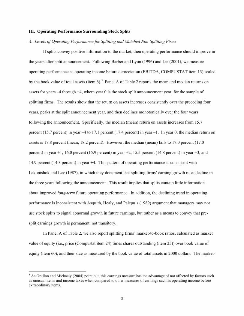
III. Operating Performance Surrounding Stock Splits

A. Levels of Operating Performance for Splitting and Matched Non-Splitting Firms

If splits convey positive information to the market, then operating performance should improve in

the years after split announcement. Following Barber and Lyon (1996) and Lie (2001), we measure

operating performance as operating income before depreciation (EBITDA, COMPUSTAT item 13) scaled

by the book value of total assets (item 6).5 Panel A of Table 2 reports the mean and median returns on

assets for years –4 through +4, where year 0 is the stock split announcement year, for the sample of

splitting firms. The results show that the return on assets increases consistently over the preceding four

years, peaks at the split announcement year, and then declines monotonically over the four years

following the announcement. Specifically, the median (mean) return on assets increases from 15.7

percent (15.7 percent) in year –4 to 17.1 percent (17.4 percent) in year –1. In year 0, the median return on

assets is 17.8 percent (mean, 18.2 percent). However, the median (mean) falls to 17.0 percent (17.0

percent) in year +1, 16.0 percent (15.9 percent) in year +2, 15.5 percent (14.8 percent) in year +3, and

14.9 percent (14.3 percent) in year +4. This pattern of operating performance is consistent with

Lakonishok and Lev (1987), in which they document that splitting firms’ earning growth rates decline in

the three years following the announcement. This result implies that splits contain little information

about improved long-term future operating performance. In addition, the declining trend in operating

performance is inconsistent with Asquith, Healy, and Palepu’s (1989) argument that managers may not

use stock splits to signal abnormal growth in future earnings, but rather as a means to convey that pre-

split earnings growth is permanent, not transitory.

In Panel A of Table 2, we also report splitting firms’ market-to-book ratios, calculated as market

value of equity (i.e., price (Compustat item 24) times shares outstanding (item 25)) over book value of

equity (item 60), and their size as measured by the book value of total assets in 2000 dollars. The market-

5 As Grullon and Michaely (2004) point out, this earnings measure has the advantage of not affected by factors such as unusual items and income taxes when compared to other measures of earnings such as operating income before extraordinary items.

9

to-book ratios follow a similar trend as that of return on assets. The median splitting firm’s market-to-

book ratio increases significantly from 1.64 four years before the split to 2.55 in the split year and then

declines to 1.99 in the fourth year after the split. The peak of market-to-book at the split year likely

reflects the result that splitting firms experience large price run-up one year prior to the announcement.

Note, however, that the market-to-book ratios after the split are larger than those before the split. As

Daniel and Titman (1999) suggest, the market-to-book (M/B) value can be used as a proxy for a

company’s growth options and higher M/B companies have more growth options. Our finding of higher

market-to-book values after splits indicate that the market continues to treat splitting firms as glamour

stocks several years after the split. Unlike the market-to-book ratio, the book value of total assets in 2000

dollars consistently increases over the nine-year period surrounding the split. The median (mean) asset

size increases from $332 million ($2,863 million) in the fourth year before the split to $803 million

($6,718 million) in the fourth year after the split.

To evaluate whether or not splitting firms’ operating performance is abnormal, we follow Barber

and Lyon (1996) and Lie (2001), and estimate expected operating performance based on a matching firm

that is selected on the basis of industry, market-to-book ratio, and past operating performance.

Specifically, we select matching firms that do not split their stock over a five-year period using the

following procedures: (1) firms that have the same two-digit SIC code as the sample firm; (2) the market-

to-book ratio is within ±20% of the sample firm’s market-to-book ratio in year −1; and (3) the return on

assets (ROA) is within ±20% of the sample firm’s ROA in year −1.6 From the firms that meet these

characteristics, we choose the firm that has ROA closest to that of the sample firm. If we cannot find any

firms that meet the criteria, we repeat the procedure first with the same one-digit SIC code as the sample

firm, and then for all firms without the use of industry classification. Just like sample firms, we also

6 Lie (2001) investigates five methods for generating control firms. Clearly, which method is more appropriate is an empirical issue. Since we do not know which method is better a priori, we tried all five methods and choose the one that gives us insignificant median absolute differences in ROA, change in ROA, and M/B between sample firms and control firms. See Lie for the detail of the five methods.

10

require the COMPUSTAT annual files to contain information on the matching firm’s operating income,

assets, and equity for all the nine years around the split announcement year (year –4 through year +4).

The operating performance, market-to-book ratio, and asset size for the matched non-splitting

firms are reported in Panel B of Table 2. The result shows that the matching firms have similar trends in

all of the three accounting measures as the sample firms, except that the median return on assets and the

market-to-book ratio both peak at the year prior to the announcement rather that the split year.

In Panel C, we report the median and mean difference of the three accounting measures between

the sample and matching firms. We test statistical significance of the median and mean difference using a

Wilcoxon matched-pair signed-rank z-statistic and a t-statistic, respectively. Compared to their matched

non-splitting firms, the splitting firms show significant better median operating performance for the nine-

year period. This better performance appears to be more pronounced in the post-split period, suggesting

that splits may contain information on improved future profitability. The market-to-book ratios and asset

sizes are also significantly higher for splitting firms, especially after the split.

B. Changes in Operating Performance for Splitting and Matched Non-Splitting Firms

Concerning about how to estimate abnormal performance, Barber and Lyon (1996) find that test

statistics using changes in operating performance are more powerful than the ones using levels. We

therefore also conduct the analysis on the changes in operating performance. Table 3, Panel A reports the

changes in return on assets of splitting firms. Although the return on assets continues to increase during

the four years until the end of the announcement year, they show a significant decline in each of the four

years following the announcement. Over the four-year pre-split period, the return on assets shows a

median (mean) increase of 1.16 percent (2.54 percent). In contrast to the pre-split period, the median

(mean) return on assets declines significantly by 2.08 percent (3.96 percent) over the four-year period

following the announcement. This finding indicates that splits signal the past rather than the future. In

other words, after several years of experiencing good operating performance, the management of a firm

11

tends to become too optimistic and splits its stock share to convey the continued good performance in the

future, if the signaling theory holds.

Table 3, Panel B reports the changes in return on asset of the splitting firms relative to the

matched non-splitting firms. The sample firms significantly outperform the matching firms for only two

years, including the year right before the announcement (year −1 to year 0) and the year right after. In

fact, the sample firms underperform their peers in the three years after year +1. If we examine the entire

four-year post-split period, the splitting firms significantly underperform their peers in terms of median

change in return on assets.

C. Changes in Liquidity for Splitting and Matched Non-Splitting Firms

While our findings on the signaling hypothesis are mixed, another view of splits is to improve

trading liquidity of a firm’s stock. As Baker and Powell’s (1992) survey research documents, the primary

motive for firms to split their stocks is to move them to an optimal trading range, followed by improving

stock trading liquidity. Thus, one plausible explanation for the positive market reaction to stock split

announcements is the increased market liquidity when firms split their shares.

The finance literature suggests a strong relation between stock split and market liquidity.

Anshuman and Kalay (2002) present a theoretical model that shows firms split their stocks to create

liquidity. Their model implies that because of price discreteness related commissions, liquidity traders

will time their trades based on stock price levels. Specifically, liquidity traders may defer their trades

until stock prices drop to lower base levels to save transaction costs. To enhance liquidity, a firm can

reset the stock price to an optimal level by splitting its stock. Empirically, a number of studies (e.g.,

Murray (1985), Muscarella and Vetsuypens (1996), and Desai, Nimalendran, and Venkataraman (1998))

find that trading activity increases after stock splits.

To assess changes in liquidity upon stock splits, we calculate a turnover ratio and an illiquidity

measure. Prior studies have used the turnover ratio as a proxy for liquidity because turnover is negatively

correlated with the bid-ask spread. The turnover ratio is calculated as the average of the daily ratio of

12

trading volume (in shares) to shares outstanding. Following Amihud (2002), the illiquidity measure is

calculated as:

ILLIQ = ∑d

d

VOLDR

N||1

, (1)

where N is the number of days for which data are available (i.e., trading volume is not zero), |Rd| is the

absolute return on day d, and VOLDd is dollar trading volume on day d. As Amihud points out, ILLIQ

measures how daily stock price reacts to a dollar of trading volume and hence is closely related to Kyle’s

(1985) concept of illiquidity, defined as the price impact of order flow. Amihud also shows that ILLIQ is

strongly positively correlated with illiquidity measures that are calculated from microstructure data. For

an economy that values liquidity, short-term abnormal returns could be due to the improved liquidity

upon stock splits. Dhar et al. (2003) find that individual investors, compared to professional investors,

trade more after splits and make up a much larger fraction of the investor base. They also find an increase

in the number of shares traded and a decrease in trade size after splits, implying improved liquidity.

Table 4 presents the two liquidity measures for the 250 trading-day period preceding the split

announcements and 250 days following the ex-dates. The mean (median) turnover ratio increases from

0.00388 (0.00229) in the pre-split period to 0.00413 (0.00231) in the post-split period (see Panel A). The

mean increase in the turnover ratio is highly significant. The illiquidity measure also suggests an

improved liquidity after the split. The mean (median) illiquidity measure declines from 0.00579

(0.00046) before the split to 0.00470 (0.00032) after the split, which is consistent with Dhar et al. (2003).

We also calculate the two liquidity measures for control firms and the results are reported in

Table 4, Panel B. The mean turnover ratio for non-splitting firms becomes smaller at the post-split

period, although the median value increases. Both the mean and median illiquidity measures decline,

suggesting that control firms also experienced improved trading liquidity.

Panel C of Table 4 presents difference in changes of liquidity measures between the splitting

firms and non-splitting firms. The mean difference in changes of turnover ratio is 0.00038 and is

statistically significant at the 10% level. Splitting firms also show slightly better improved liquidity

13

based on daily stock price reactions to a dollar of trading volume, though the difference is not statistically

significant.

IV. Split Signals, Changes in Operating Performance and Liquidity, and Excess Returns

A. Split Signals and Changes in Operating Performance

In this sub-section, we examine whether splits contain information content by regressing future

profitability of a splitting firm on a variable that is used as a proxy for the signal of management’s split

decision and various control variables. If the signaling hypothesis holds, the split signal will be positively

related to future operating performance and will add some explanatory power to predicting future

profitability.

According to the signaling hypothesis, managers use stock splits to reveal favorable private

information about the firm’s improved future profitability. To extract management’s private information

about the firm’s performance contained in splits, we specify a group of factors that may affect the split

decision. Following McNichols and Dravid (1990) and Nayak and Prabhala (2001), the following probit

regression model is used:

SPLi = α0 + α1RUNUPi + α2PR_PRICEi + α3MVi + α4∆ROA-1,i + α5PR_ILLIQi + ψi, (2)

where SPLi is a latent variable that is 1.0 for the splitting firms and zero for the matched non-splitting

firms, RUNUPi is the price run-up as reported in Table 1, PR_PRICEi is firm i’s share price five trading

days before the split, MVi is the natural logarithm of the market value of the firm five trading days prior

to the split, ∆ROA-1,i is change in ROA in year −1, PR_ILLIQi is pre-split illiquidity measure as reported

in Table 4, and ψi is the regression residual. The variable PR_PRICE is included because firms with

higher share prices are more likely to split. Similarly, we include the variable RUNUP to capture the

observation that splits are usually made by firms with large price increases. We include the market value

of firm (MV) as a control variable, since larger firms might prefer to maintain higher share prices. ∆ROA

14

is included to control for pre-split operating performance changes. PR_ILLIQ is included because firms

with higher pre-split illiquidity may have more incentive to split.

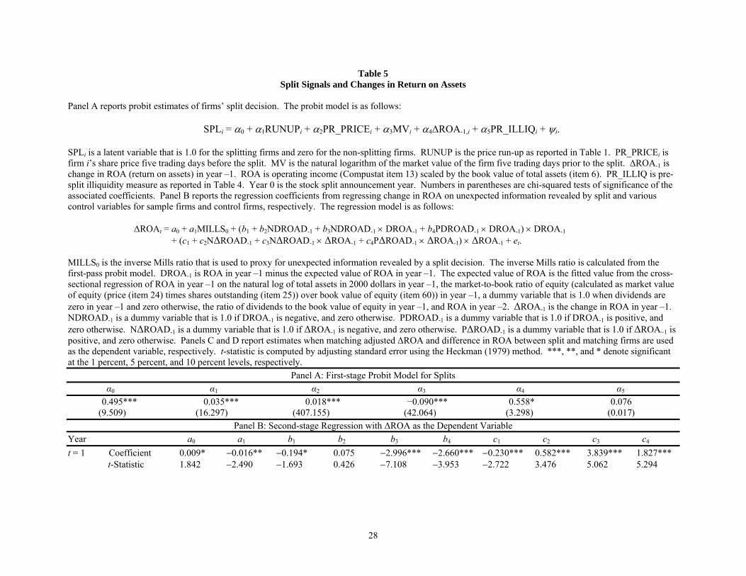
Panel A of Table 5 reports the estimates from the probit model. The coefficient for RUNUP is

positive and highly significant, indicating that typically firms split when they have performed well in the

market. The coefficient for PR_PRICE is positive and highly significant, suggesting that splitting firms

tend to have a high stock price. Consistent with McNichols and Dravid (1990) and Nayak and Prabhala

(2001), the coefficient for the market size variable is negative, implying that small firms are more likely

to split than do large firms. The coefficient for ∆ROA-1 is positive, which suggests that firms with larger

change in return on assets are more likely to announce splits. Consistent with the view of improved

liquidity, the coefficient for illiquidity measure is positive, though is not statistically significant.

As Nayak and Prabhala (2001) point out, under the assumption that ψi is standard normal, a

firm’s decision to split can be described as a standard probit model as Equation (2). Using the probit

estimates from Equation (2), we then calculate the inverse Mills ratio for splitting firms that can be seen

as a splitter’s private information not known to the market when a split is made, and is used as a proxy for

the signal of management’s favorable private information. If the signaling hypothesis holds, the split

signal should be positively related to changes in future profitability.

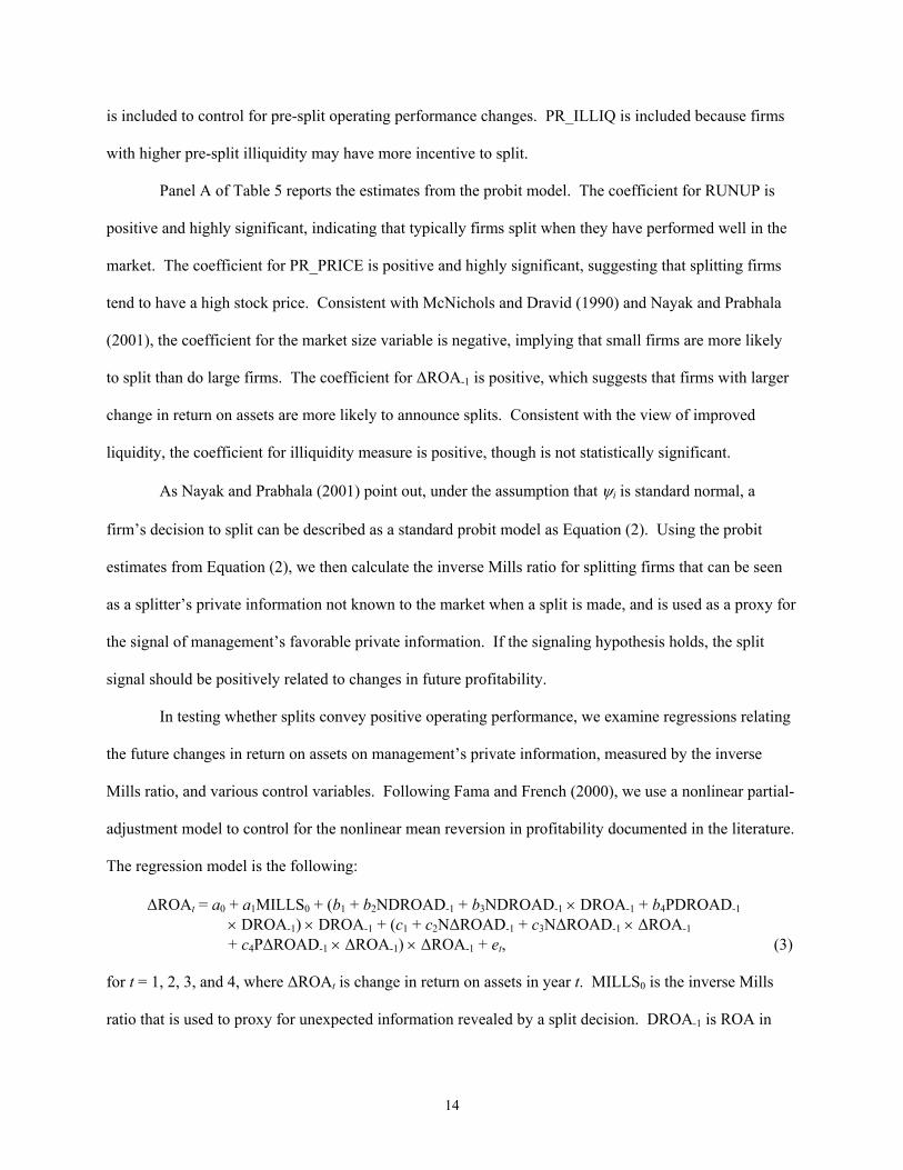
In testing whether splits convey positive operating performance, we examine regressions relating

the future changes in return on assets on management’s private information, measured by the inverse

Mills ratio, and various control variables. Following Fama and French (2000), we use a nonlinear partial-

adjustment model to control for the nonlinear mean reversion in profitability documented in the literature.

The regression model is the following:

∆ROAt = a0 + a1MILLS0 + (b1 + b2NDROAD-1 + b3NDROAD-1 × DROA-1 + b4PDROAD-1 × DROA-1) × DROA-1 + (c1 + c2N∆ROAD-1 + c3N∆ROAD-1 × ∆ROA-1 + c4P∆ROAD-1 × ∆ROA-1) × ∆ROA-1 + et, (3) for t = 1, 2, 3, and 4, where ∆ROAt is change in return on assets in year t. MILLS0 is the inverse Mills

ratio that is used to proxy for unexpected information revealed by a split decision. DROA-1 is ROA in

15

year –1 minus the expected value of ROA in year –1. The expected value of ROA is the fitted value from

the cross-sectional regression of ROA in year –1 on the natural log of total assets in 2000 dollars in year –

1, the market-to-book ratio in year –1, a dummy variable that is 1.0 when dividends are zero in year –1

and zero otherwise, the ratio of dividends to the book value of equity in year –1, and ROA in year –2.

∆ROA is the change in ROA in year –1. NDROAD-1 is a dummy variable that is 1.0 if DROA-1 is

negative, and zero otherwise. PDROAD-1 is a dummy variable that is 1.0 if DROA-1 is positive, and zero

otherwise. N∆ROAD-1 is a dummy variable that is 1.0 if ∆ROA-1 is negative, and zero otherwise.

P∆ROAD-1 is a dummy variable that is 1.0 if ∆ROA-1 is positive, and zero otherwise. The coefficient b1

measures mean reversion in operating performance. The coefficients b2, b3, and b4 are to measure

nonlinear mean reversion in operating performance, meaning that the reversals are stronger for large

changes of either sign. The coefficient c1 measures partial adjustment effect. The coefficients c2, c3, and

c4 measure stronger nonlinear mean reversion in operating performance for negative changes.

Since the inverse Mills ratio is a calculated variable, an errors-in-variables problem will arise in

the estimation of equation (3) and hence the standard errors are inconsistent. We estimate consistent

standard errors using Heckman’s (1979) two-stage method that was generalized by Greene (1981). The

results reported in Table 5, Panel B show that the split signal coefficient is positive only in year +2, but is

negative in years +1, +3, and +4, which are inconsistent with the signaling model’s prediction. This

finding suggests that stock split announcements do not contain favorable information content about future

operating performance. Consistent with Fama and French (2000), the regression coefficient on the return

on assets in year –1, DROA-1, is negative for the regression specification in years +1, +2, and +4,

indicating that operating performance reverts to mean. Moreover, most estimates of b’s and c’s are

strongly significant.

Since a better way of judging future profitability is to compare it with a matched firm, we also

examine whether splits convey operating performance improvements using matching adjusted change in

ROA as the dependent variable. Table 5, Panel C reports the regression results. The coefficient on the

16

inverse Mills ratio is positive only for years +1 and +4. Nevertheless, none of the two positive coefficient

estimates are significant.

The results reported in Table 2 indicates that splitting firms experience better operating

performances after split compared to matching non-splitting firms. The result suggests that splits may

signal performance improvement in the level of ROA rather than in change in ROA. To investigate this,

we rerun regression with difference in ROA between the split and matching firms as the dependent

variable. Panel D of Table 5 shows that the association between the split signal and the difference in

ROA between the split and matching firms is positive but insignificant in year +1. For the other three

years, the coefficients on the split signal are all negative.

B. Announcement Period Excess Returns, Changes in Profitability and Liquidity, and Share Price

Prior studies have linked excess returns surrounding the split announcement with management’s

optimism about the future. If the signaling hypothesis holds, the excess returns should be positively

related to changes in profitability. Another explanation for the positive market reaction is that splits

effectively reduce share price and improve trading liquidity. If firms split their shares intend to improve

market liquidity and if liquidity is priced, we would expect to see that the short-term announcement effect

to be explained (at least partially) by the improved trading liquidity. Specifically, if liquidity premium is

a component of equity premium in asset pricing, then there should be a positive relation between stock

return and market illiquidity. Thus, an improved liquidity (or lower illiquidity) following stock splits will

raise stock price due to the decrease in a firm’s equity risk premium and its cost of capital, generating a

positive market reaction. To examine these relations, we regress excess return surrounding the

announcement on changes in profitability, changes in trading liquidity, unexpected information revealed

by split, and various control variables. The regression model is:

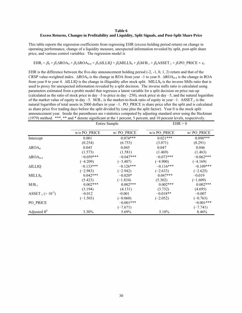
EHRt = β0 + β1∆ROA0 + β2∆ROA0-4 + β3∆ILLIQ + β4MILLS0 + β5M/B-1 + β6ASSET-1 + εt. (4)

17

EHR is the difference between the five-day announcement holding period (−2, −1, 0, 1, 2) return and that

of the CRSP value-weighted index. ∆ROA0 is the change in ROA from year –1 to year 0. ∆ROA0-4 is the

change in ROA from year 0 to year +4. We use ∆ROA0 and ∆ROA0-4 to proxy for changes in operating

performance.7 A positive and significant coefficient for ∆ROA0-4 would indicate that the announcement

effect reflects improved future operating performance. ∆ILLIQ is the change in illiquidity measure as

reported in Table 4, Panel A. The improved liquidity hypothesis suggests that the coefficient of ∆ILLIQ

should be positive. MILLS0 is the inverse Mills ratio, which is calculated using parameters estimated

from the probit model (2), and is used to proxy for unexpected information revealed by a split decision. If

the coefficient for MILLS0 is positive and significant, then splits convey additional positive information

content than improved profitability and liquidity. M/B−1 is the market-to-book ratio of equity in year –1.

ASSET-1 is the natural logarithm of total assets in 1996 dollars in year –1. The market-to-book ratio and

asset size are included as additional variables to control for possible information asymmetry.

The results reported in Table 6 (column 1) show that a negative coefficient of ∆ROA0-4,

indicating that the announcement excess return cannot be explained by the operating performance during

the four-year period following the announcement. This result, coupled with the findings reported above

that splits do not signal improved operating performance, does not support the prediction of the signaling

hypothesis. However, the estimated coefficient of ∆ILLIQ is negative and highly significant, suggesting

that lower illiquidity leads to higher stock returns. Thus, the positive market reaction seems to be more

consistent with the improved liquidity hypothesis. Nevertheless, the positive and significant coefficient

of the split signal, MILLS0, implies that a large portion of the announcement effect cannot be explained

by the improved liquidity. We also find a stronger relation between the market reaction and the liquidity

measure for firms with larger market-to-book value.

7 To check for the robustness of the result, we also use adjusted ∆ROA, which is equal to the change in ROA of a splitting firm minus the change in ROA of a matching firm, in the analysis. The results are qualitatively the same.

18

Our finding is clearly inconsistent with the suggestion that managers use splits to signal favorable

private information on their firms’ future prospect. In the meantime, it is also unclear what information

content is conveyed in the split signal beyond improved trading liquidity. In fact, prior survey studies

(see, for example, Baker and Gallagher (1980) and Baker and Powell (1992)) cite that realigning share

prices to lower trading ranges is the main motive for corporations to conduct a stock split. The

specifications in Equation (4), however, do not enable us to assess the possibility that the realignment of

share price explains some part of the market reaction. In addition, Brennan and Hughes (1991) suggest

that the split ratio itself is an informative signal, especially for splits that result in low post-split share

prices. To examine this, we re-estimate Equation (4) by adding post-split price, PO_PRICE, as an

additional variable. PO_PRICE is share price after the split and is calculated as share price five trading

days before the split divided by (one plus the split factor). If the primary motivation behind a split is to

return the share price to a lower range, we should observe a negative coefficient for PO_PRICE, meaning

that the market reacts more positively to lower price after the split.

As expected, the split announcement is negatively related to the post-split stock price (column 2,

Table 6). More importantly, the coefficient of MILLS0 changes from a positive number to a negative

number, while other coefficients remain qualitatively the same when compared to those in column 1.

This finding suggests that the positive market reaction is mainly due to the realignment of share prices

and the improved liquidity, which is consistent with prior survey results (Baker and Gallagher (1980) and

Baker and Powell (1992)) and with the main conclusion of Lakonishok and Lev (1987).

Clearly not all splitting firms experience a positive market reaction. Indeed, about 27.6% of firms

do not exhibit a positive effect upon the split announcement. As a diagnostic, we redo the analysis using

only the sample firms that show a positive announcement effect. The results are shown in columns 3 and

4 in Table 6. As can be seen, the results are qualitatively the same as those from analyzing the entire

sample. That is, like the entire sample, the positive announcement effect can only be explained by lower

share price after the split and improved trading liquidity but not by changes in future profitability.

19

V. Conclusions

In this study, we examine whether firms split their stock shares to signal higher future

profitability to the market or to adjust share prices to a desired trading range in order to improve trading

liquidity, or both. Using a sample of 2,335 stock splits over the 1963-1999 period, we find that the split

announcement year has the highest operating performance change and the operating performance change

declines substantially over the subsequent four years. However, we do find evidence of improved

operating performance when comparing splitting firms to their matching peers. Nevertheless, our

regression analysis shows a negative relation between the split signal and most future operating

performance following the announcement, regardless of the measures of operating performance that we

use. We also find a negative relation between the stock split announcement effect and the operating

performance during the four-year period following the announcement.

Our results show improved market liquidity following stock splits. This improved liquidity also

significantly explains the stock split announcement effect. More importantly, we find that the alignment

of share prices to lower price ranges not only significantly explains the announcement effect, but renders

the significant explanatory power of the split signals to become much less significant and reverse the sign

of the coefficient estimate. In short, our results appear to suggest that the positive announcement effect is

more consistent with the trading range/liquidity hypothesis rather than with the signaling hypothesis.

20

References

Admati, A. R., and P. Pfleiderer, 1988, “A theory of intraday patterns: Volume and price variability,”

Review of Financial Studies 1, 3-40.

Amihud, Y., 2002, “Illiquidity and stock returns: Cross-section and time-series effects,” Journal of

Financial Markets 5, 31-56.

Angel, J. J., 1997, “Tick size, share prices and stock splits,” Journal of Finance 52, 655-681.

Anshuman, V. R., and A. Kalay, 2002, “Can splits create market liquidity? Theory and evidence,”

Journal of Financial Markets 5, 83-125.

Asquith, O., P. Healy, and K. Palepu, 1989, “Earnings and stock splits,” Accounting Review 64, 387-403.

Baker, H. K., and P. L. Gallagher, 1980, “Management’s view of stock splits,” Financial Management 9,

73-77.

Baker, H. K., and G. E. Powell, 1992, “Why companies issue stock splits,” Financial Management 21,

11.

Barber, B. M., and J. D. Lyon, 1996, “Detecting abnormal operating performance: The empirical power

and specification of test statistics,” Journal of Financial Economics 41, 359-399.

Brennan, M. J., and T. E. Copeland, 1988, “Stock splits, stock prices, and transaction costs,” Journal of

Financial Economics 22, 83-101.

Brennan, M. J., and P. J. Hughes, 1991, “Stock prices and the supply of information,” Journal of Finance

46, 1665-1691.

Byun, J., and M. S. Rozeff, 2003, “Long-run performance after stock splits: 1927 to 1996,” Journal of

Finance 58, 1063-1085.

Conroy, J. S., R. S. Harris, and B. A. Benet, 1990, “The effects of stock splits on bid-ask spreads,”

Journal of Finance 45, 1285-1295.

Copeland, T. E., 1979, “Liquidity changes following stock splits,” Journal of Finance 34, 115-141.

Daniel, K., and S. Titman, 1999, “Market Efficiency in an irrational world,” Financial Analysts Journal

55, 28-40.

21

Desai, A. S., M. Nimalendran, and S. Venkataraman, 1998, “Changes in trading activity following stock

splits and their effect on volatility and the adverse-information component of the bid-ask spread,”

Journal of Financial Research 21, 159-183.

Desai, H., and P. C. Jain, 1997, “Long-run common stock returns following stock splits and reverse

splits,” Journal of Business 70, 409-433,

Dhar, R., W. N. Goetzmann, S. Shepherd, and N. Zhu, 2003, “The impact of clientele changes: Evidence

from stock splits,” working paper, Yale University.

Dubofsky, D. A., 1991, “Volatility increases subsequent to NYSE and AMEX stock splits,” Journal of

Finance 46, 421-431.

Easley, D., M. O’Hara, and G. Saar, 2001, “How stock splits affect trading: A microstructure approach,”

Journal of Financial and Quantitative Analysis 36, 25-51.

Fama, E. F., and K. R. French, 2000, “Forecasting profitability and earnings,” Journal of Business 73,

161-175.

Greene, W., 1981, “Sample Selection Bias as a Specification Error: Comment,” Econometrica 49, 795-

798.

Grinblatt, M. S., R. W. Masulis, and S. Titman, 1984, “The valuation effects of stock splits and stock

dividends,” Journal of Financial Economics 13, 461-490.

Grullon, G., and R. Michaely, 2004, “The information content of share repurchase programs,” Journal of

Finance 59, 651-680.

Heckman, J., 1979, “Sample Selection Bias as a Specification Error,” Econometrica 47, 153-161.

Ikenberry, D. L., G. Rankine, and E. K. Stice, 1996, “What do stock splits really signal?” Journal of

Financial and Quantitative Analysis 31, 357-375.

Ikenberry, D. L., and S. Ramnath, 2002, “Underreaction to self-selected news events: The case of stock

split,” Review of Financial Studies 15, 489-526.

Kyle, A. S., 1985, “Continuous auctions and insider trading,” Econometrica 53, 1315-1335.

22

Lakonishok, J., and B. Lev, 1987, “Stock splits and stock dividends: Why, who, and when,” Journal of

Finance 42, 913-932.

Lamoureux, C. G., and P. Poon, 1987, “The market reaction to stock splits,” Journal of Finance 42, 1347-

1370.

Lie, E., 2001, “Detecting abnormal operating performance: Revisited,” Financial Management 30, 77-91.

Loughran, T., and J. R. Ritter, 1997, “The operating performance of firms conducting seasoned equity

offerings,” Journal of Finance 52, 1823-1850.

McNichols, M., and A. Dravid, 1990, “Stock dividends, stock splits, and signaling,” Journal of Finance

45, 857-879.

Murray, D., 1985, “Further evidence on the liquidity effects of stock splits and stock dividends,” Journal

of Financial Research 8, 59-67.

Muscarella, C., and M. Vetsuypens, 1996, “Stock splits: Signaling or liquidity? the case of ADR ‘solo

splits’,” Journal of Financial Economics 42, 3-26.

Nayak, S., and N. R. Prabhala, 2001, “Disentangling the dividend information in splits: A decomposition

using conditional event-study methods,” Review of Financial Studies 14, 1083-1116.

Powell, G. E., and H. K. Baker, 1993/1994, “The effects of stock splits on the ownership mix of a firm,”

Review of Financial Economics 3, 70-88.

Schultz, P., 2000, “Stock splits, tick size, and sponsorship,” Journal of Finance 55, 429-450.

23

Table 1 Description of Sample

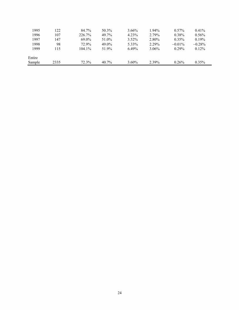
This table describes the stock split sample used in the current study. To be included in the sample, a splitting firm needs to wait for five years before it can reenter the stock split sample. The sample period is 1963-1999. RUNUP is rate of return calculated using the price of a firm’s stock five trading days prior to the split and the price one year before the split. EHR is the difference between the five-day announcement holding period (-2, -1, 0, 1, 2) return of a sample firm and that of the CRSP value-weighted index. CRSP is the five-day announcement holding period return for the CRSP value-weighted index

Panel A: By split ratio Split Ratio Number of Splits Three-for-One 123 Two-for-One 1264 Three-for-Two 682 Four-for-Three 45 Five-for-Four 144 Other 77 Total 2335

Panel B: By year Number of RUNUP EHR CRSP_________ Year Splits Mean Median Mean Median Mean Median 1963 5 50.1% 38.8% 1.82% 1.14% 1.13% 1.24% 1964 15 35.7% 35.8% −0.31% −0.41% 0.32% 0.28% 1965 26 30.6% 21.5% 2.87% 2.49% 0.25% 0.42% 1966 25 55.9% 38.0% 3.20% 3.14% −0.13% −0.27% 1967 16 85.0% 48.9% 3.01% 2.84% −0.01% 0.20% 1968 25 58.0% 30.1% 2.19% 1.82% −0.30% −0.25% 1969 28 47.0% 24.8% 1.45% 1.39% −0.08% 0.45% 1970 16 29.7% 3.6% 1.85% 1.45% 1.21% 1.44% 1971 25 90.3% 43.5% 2.91% 3.39% 0.58% 0.55% 1972 31 39.1% 40.6% 1.42% 1.88% 0.39% 0.77% 1973 30 33.9% 28.8% 2.71% 2.49% −0.77% −1.47% 1974 4 68.3% 58.1% 1.39% 3.58% −1.64% −2.34% 1975 6 52.4% 36.9% 1.66% 1.10% −1.55% −1.48% 1976 17 41.8% 40.9% 3.64% 2.48% 0.52% 0.47% 1977 32 31.6% 20.2% 4.55% 3.63% 0.24% 0.62% 1978 32 60.0% 46.8% 2.84% 3.18% 0.17% 0.52% 1979 22 47.5% 36.0% 4.00% 4.74% −0.03% 0.12% 1980 50 77.8% 59.0% 4.22% 3.37% 0.61% 1.17% 1981 36 61.2% 47.2% 2.49% 2.35% −0.97% −0.67% 1982 30 50.2% 49.0% 3.96% 1.65% 0.47% 0.13% 1983 144 139.4% 100.9% 5.67% 4.15% 0.43% 0.46% 1984 81 20.1% 9.0% 3.19% 2.75% 0.23% −0.10% 1985 86 42.6% 36.6% 3.64% 2.67% 0.42% 0.55% 1986 135 54.9% 42.2% 3.21% 2.23% 0.47% 0.72% 1987 129 47.1% 31.2% 3.07% 2.06% 0.45% 0.68% 1988 62 17.3% 10.7% 3.09% 2.08% 0.51% 0.77% 1989 95 52.6% 37.1% 2.65% 1.55% 0.47% 0.70% 1990 62 52.6% 27.9% 2.28% 1.74% −0.31% −0.14% 1991 85 72.4% 45.1% 4.48% 2.42% 0.44% 0.42% 1992 164 73.7% 48.3% 3.30% 2.19% 0.11% 0.20% 1993 145 67.8% 38.6% 3.26% 2.01% 0.25% 0.42% 1994 87 42.3% 22.2% 2.06% 1.16% −0.10% 0.03%

24

1995 122 84.7% 50.3% 3.66% 1.94% 0.57% 0.41% 1996 107 226.7% 49.7% 4.23% 2.79% 0.38% 0.56% 1997 147 69.0% 51.0% 3.52% 2.80% 0.35% 0.19% 1998 98 72.9% 49.0% 5.33% 2.29% −0.01% −0.28% 1999 115 104.1% 51.9% 6.49% 3.06% 0.29% 0.12% Entire Sample 2335 72.3% 40.7% 3.60% 2.39% 0.26% 0.35%

25

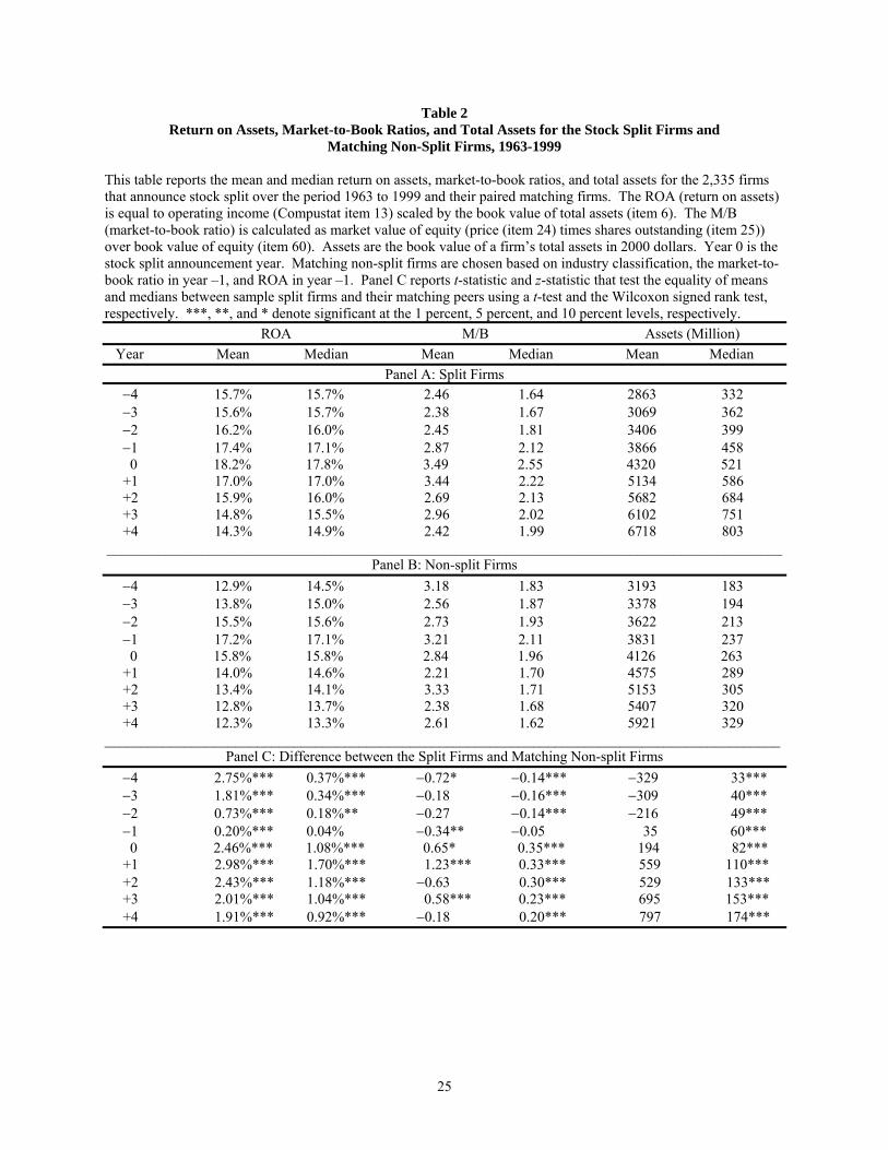
Table 2 Return on Assets, Market-to-Book Ratios, and Total Assets for the Stock Split Firms and

Matching Non-Split Firms, 1963-1999 This table reports the mean and median return on assets, market-to-book ratios, and total assets for the 2,335 firms that announce stock split over the period 1963 to 1999 and their paired matching firms. The ROA (return on assets) is equal to operating income (Compustat item 13) scaled by the book value of total assets (item 6). The M/B (market-to-book ratio) is calculated as market value of equity (price (item 24) times shares outstanding (item 25)) over book value of equity (item 60). Assets are the book value of a firm’s total assets in 2000 dollars. Year 0 is the stock split announcement year. Matching non-split firms are chosen based on industry classification, the market-to-book ratio in year –1, and ROA in year –1. Panel C reports t-statistic and z-statistic that test the equality of means and medians between sample split firms and their matching peers using a t-test and the Wilcoxon signed rank test, respectively. ***, **, and * denote significant at the 1 percent, 5 percent, and 10 percent levels, respectively. ROA M/B Assets (Million) Year Mean Median Mean Median Mean Median

Panel A: Split Firms −4 15.7% 15.7% 2.46 1.64 2863 332 −3 15.6% 15.7% 2.38 1.67 3069 362 −2 16.2% 16.0% 2.45 1.81 3406 399 −1 17.4% 17.1% 2.87 2.12 3866 458 0 18.2% 17.8% 3.49 2.55 4320 521 +1 17.0% 17.0% 3.44 2.22 5134 586 +2 15.9% 16.0% 2.69 2.13 5682 684 +3 14.8% 15.5% 2.96 2.02 6102 751 +4 14.3% 14.9% 2.42 1.99 6718 803 _____________________________________________________________________________________________

Panel B: Non-split Firms −4 12.9% 14.5% 3.18 1.83 3193 183 −3 13.8% 15.0% 2.56 1.87 3378 194 −2 15.5% 15.6% 2.73 1.93 3622 213 −1 17.2% 17.1% 3.21 2.11 3831 237 0 15.8% 15.8% 2.84 1.96 4126 263 +1 14.0% 14.6% 2.21 1.70 4575 289 +2 13.4% 14.1% 3.33 1.71 5153 305 +3 12.8% 13.7% 2.38 1.68 5407 320 +4 12.3% 13.3% 2.61 1.62 5921 329 _____________________________________________________________________________________________

Panel C: Difference between the Split Firms and Matching Non-split Firms −4 2.75%*** 0.37%*** −0.72* −0.14*** −329 33*** −3 1.81%*** 0.34%*** −0.18 −0.16*** −309 40*** −2 0.73%*** 0.18%** −0.27 −0.14*** −216 49*** −1 0.20%*** 0.04% −0.34** −0.05 35 60*** 0 2.46%*** 1.08%*** 0.65* 0.35*** 194 82*** +1 2.98%*** 1.70%*** 1.23*** 0.33*** 559 110*** +2 2.43%*** 1.18%*** −0.63 0.30*** 529 133*** +3 2.01%*** 1.04%*** 0.58*** 0.23*** 695 153*** +4 1.91%*** 0.92%*** −0.18 0.20*** 797 174***

26

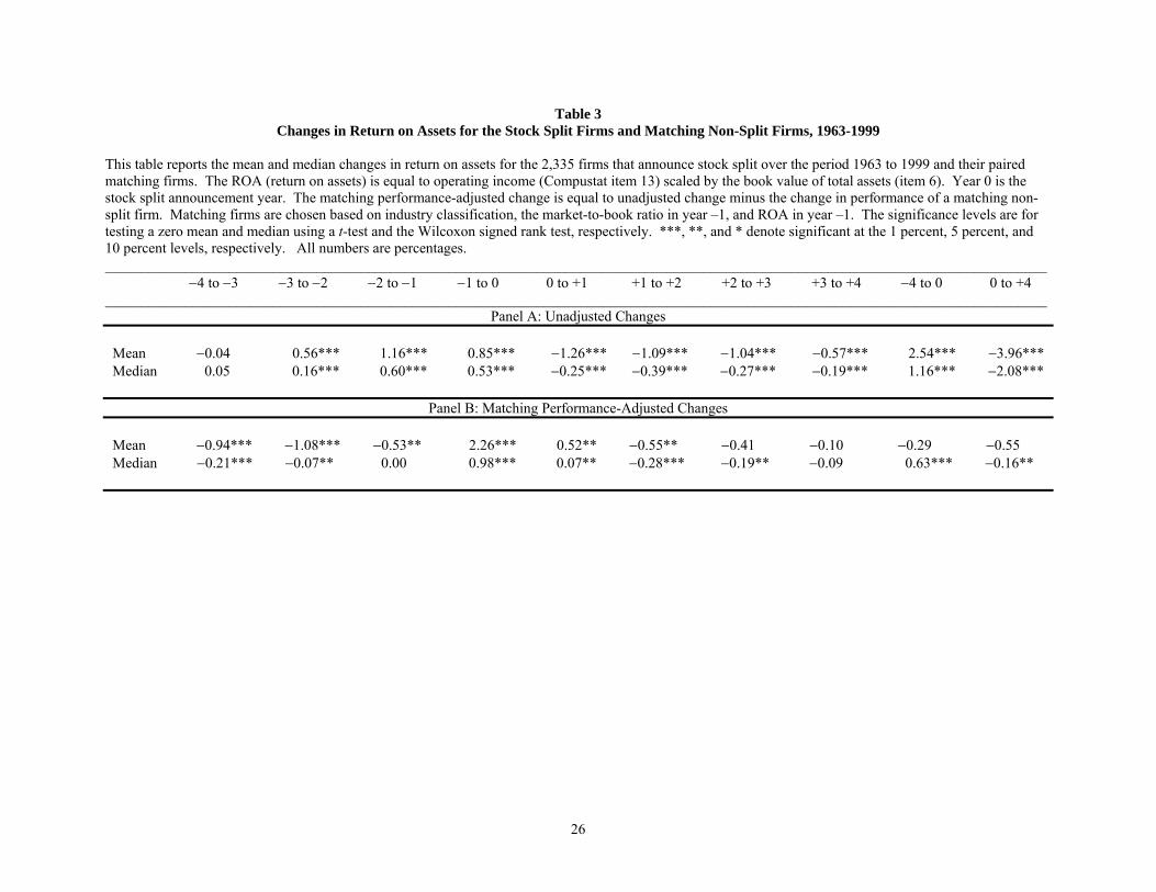
Table 3 Changes in Return on Assets for the Stock Split Firms and Matching Non-Split Firms, 1963-1999

This table reports the mean and median changes in return on assets for the 2,335 firms that announce stock split over the period 1963 to 1999 and their paired matching firms. The ROA (return on assets) is equal to operating income (Compustat item 13) scaled by the book value of total assets (item 6). Year 0 is the stock split announcement year. The matching performance-adjusted change is equal to unadjusted change minus the change in performance of a matching non-split firm. Matching firms are chosen based on industry classification, the market-to-book ratio in year –1, and ROA in year –1. The significance levels are for testing a zero mean and median using a t-test and the Wilcoxon signed rank test, respectively. ***, **, and * denote significant at the 1 percent, 5 percent, and 10 percent levels, respectively. All numbers are percentages. _________________________________________________________________________________________________________________________________ −4 to −3 −3 to −2 −2 to −1 −1 to 0 0 to +1 +1 to +2 +2 to +3 +3 to +4 −4 to 0 0 to +4 _________________________________________________________________________________________________________________________________

Panel A: Unadjusted Changes Mean −0.04 0.56*** 1.16*** 0.85*** −1.26*** −1.09*** −1.04*** −0.57*** 2.54*** −3.96*** Median 0.05 0.16*** 0.60*** 0.53*** −0.25*** −0.39*** −0.27*** −0.19*** 1.16*** −2.08***

Panel B: Matching Performance-Adjusted Changes

Mean −0.94*** −1.08*** −0.53** 2.26*** 0.52** −0.55** −0.41 −0.10 −0.29 −0.55 Median −0.21*** −0.07** 0.00 0.98*** 0.07** −0.28*** −0.19** −0.09 0.63*** −0.16**

27

Table 4 Changes in Liquidity for the Sample Splitting Firms and Matching Non-Split Firms, 1963-1999

This table reports two liquidity measures for the 2,335 firms that announced stock split over the period 1963 to 1999 and their paired matching firms. Pre-split measures are estimated over the 250 trading-day period preceding the split announcements, while post-split measures are estimated over the 250 days following the ex-dates. Turnover ratio is the average of the daily ratio of stock trading volume (in shares) to the shares outstanding. Illiquidity is the average of the ratio of a stock’s daily absolute return to its dollar trading volume. The significance levels are for testing a zero mean and median using a t-test and the Wilcoxon signed rank test, respectively. ***, **, and * denote significant at the 1 percent, 5 percent, and 10 percent levels, respectively. Liquidity Measures Pre-Split Period Post-Split Period Change

Panel A: Split Firms Turnover Ratio (× 102) Mean 0.388 0.413 0.025** Median 0.229 0.231 −0.004** Illiquidity (× 102) Mean 0.579 0.470 −0.109 Median 0.046 0.032 −0.001***

Panel B: Non-split Firms Turnover Ratio (× 102) Mean 0.374 0.361 −0.013 Median 0.217 0.219 −0.000 Illiquidity (× 102) Mean 3.205 3.154 −0.051 Median 0.141 0.121 −0.001***

Panel C: Difference in Changes between the Split Firms and Matching Non-split Firms Turnover Ratio (× 102) Mean 0.038* Median −0.003 Illiquidity (× 102) Mean −0.057 Median −0.000

28

Table 5 Split Signals and Changes in Return on Assets

Panel A reports probit estimates of firms’ split decision. The probit model is as follows: SPLi = α0 + α1RUNUPi + α2PR_PRICEi + α3MVi + α4∆ROA-1,i + α5PR_ILLIQi + ψi. SPLi is a latent variable that is 1.0 for the splitting firms and zero for the non-splitting firms. RUNUP is the price run-up as reported in Table 1. PR_PRICEi is firm i’s share price five trading days before the split. MV is the natural logarithm of the market value of the firm five trading days prior to the split. ∆ROA-1 is change in ROA (return on assets) in year –1. ROA is operating income (Compustat item 13) scaled by the book value of total assets (item 6). PR_ILLIQ is pre-split illiquidity measure as reported in Table 4. Year 0 is the stock split announcement year. Numbers in parentheses are chi-squared tests of significance of the associated coefficients. Panel B reports the regression coefficients from regressing change in ROA on unexpected information revealed by split and various control variables for sample firms and control firms, respectively. The regression model is as follows: ∆ROAt = a0 + a1MILLS0 + (b1 + b2NDROAD-1 + b3NDROAD-1 × DROA-1 + b4PDROAD-1 × DROA-1) × DROA-1 + (c1 + c2N∆ROAD-1 + c3N∆ROAD-1 × ∆ROA-1 + c4P∆ROAD-1 × ∆ROA-1) × ∆ROA-1 + et. MILLS0 is the inverse Mills ratio that is used to proxy for unexpected information revealed by a split decision. The inverse Mills ratio is calculated from the first-pass probit model. DROA-1 is ROA in year –1 minus the expected value of ROA in year –1. The expected value of ROA is the fitted value from the cross-sectional regression of ROA in year –1 on the natural log of total assets in 2000 dollars in year –1, the market-to-book ratio of equity (calculated as market value of equity (price (item 24) times shares outstanding (item 25)) over book value of equity (item 60)) in year –1, a dummy variable that is 1.0 when dividends are zero in year –1 and zero otherwise, the ratio of dividends to the book value of equity in year –1, and ROA in year –2. ∆ROA-1 is the change in ROA in year –1. NDROAD-1 is a dummy variable that is 1.0 if DROA-1 is negative, and zero otherwise. PDROAD-1 is a dummy variable that is 1.0 if DROA-1 is positive, and zero otherwise. N∆ROAD-1 is a dummy variable that is 1.0 if ∆ROA-1 is negative, and zero otherwise. P∆ROAD-1 is a dummy variable that is 1.0 if ∆ROA−1 is positive, and zero otherwise. Panels C and D report estimates when matching adjusted ∆ROA and difference in ROA between split and matching firms are used as the dependent variable, respectively. t-statistic is computed by adjusting standard error using the Heckman (1979) method. ***, **, and * denote significant at the 1 percent, 5 percent, and 10 percent levels, respectively.

Panel A: First-stage Probit Model for Splits α0 α1 α2 α3 α4 α5

0.495*** 0.035*** 0.018*** −0.090*** 0.558* 0.076 (9.509) (16.297) (407.155) (42.064) (3.298) (0.017)

Panel B: Second-stage Regression with ∆ROA as the Dependent Variable Year a0 a1 b1 b2 b3 b4 c1 c2 c3 c4 t = 1 Coefficient 0.009* −0.016** −0.194* 0.075 −2.996*** −2.660*** −0.230*** 0.582*** 3.839*** 1.827*** t-Statistic 1.842 −2.490 −1.693 0.426 −7.108 −3.953 −2.722 3.476 5.062 5.294

29

t = 2 Coefficient −0.009* 0.005 −0.295** 0.238 0.056 3.315*** −0.104 −0.058 −1.405* −1.700*** t-Statistic −1.870 0.733 −2.461 1.293 0.127 4.697 −1.174 −0.330 −1.763 −4.695 t = 3 Coefficient −0.002 −0.008 0.216 −0.836*** −6.608*** −1.607* −0.425*** 0.963*** 5.791*** 1.936*** t-Statistic −0.373 −1.073 1.546 −3.901 −12.798 −1.953 −4.113 4.696 6.230 4.585 t = 4 Coefficient 0.008 −0.016* −0.515*** 0.938*** 2.564*** 1.938* 0.421*** −0.726*** −2.079* −1.749*** t-Statistic 1.125 −1.659 −3.018 3.589 4.074 1.931 3.339 −2.903 −1.835 −3.396

Panel C: Second-pass Regression with Matching Adjusted ∆ROA as the Dependent Variable Year a0 a1 b1 b2 b3 b4 c1 c2 c3 c4 t = 1 Coefficient 0.016* 0.004 0.241 0.334 −0.853 −0.308 −0.516*** 0.249 0.724 0.702 t-Statistic 1.909 0.385 1.166 1.056 −1.120 −0.254 −3.391 0.824 0.528 1.127 t = 2 Coefficient −0.004 −0.003 −0.968*** 0.801** −0.931 7.050*** 0.530*** −0.694** 0.296 −3.511*** t-Statistic −0.381 −0.233 −4.077 2.204 −1.063 5.050 3.022 −1.993 0.188 −4.901 t = 3 Coefficient −0.002 −0.006 0.517** −1.185*** −6.947*** −2.313* −0.511*** 0.824** 4.684*** 2.145*** t-Statistic −0.234 −0.479 2.313 −3.457 −8.415 −1.758 −3.077 2.513 3.152 3.177 t = 4 Coefficient 0.003 0.002 0.001 0.780* 2.556*** −3.214** 0.158 −0.639* −0.429 0.498 t-Statistic 0.103 0.103 0.001 1.939 2.636 −2.080 0.815 −1.658 −0.246 0.628

Panel D: Second-pass Regression with Difference in ROA between Split and Matching Firms as the Dependent Variable Year a0 a1 b1 b2 b3 b4 c1 c2 c3 c4 t = 1 Coefficient 0.033*** 0.001 0.751*** −0.474 −1.885** −2.822* −0.507*** 0.023 0.240 0.364 t-Statistic 3.226 0.036 2.960 −1.221 −2.014 −1.892 −2.708 0.062 0.140 0.476 t = 2 Coefficient 0.029*** −0.003 −0.217 0.327 −2.816*** 4.228*** 0.023 −0.671* 0.536 −3.147*** t-Statistic 2.850 −0.181 −0.850 0.836 −2.989 2.815 0.120 −1.792 0.316 −4.084 t = 3 Coefficient 0.027** −0.008 0.300 −0.858* −9.763*** 1.914 −0.489** 0.153 5.220*** −1.002 t-Statistic 2.312 −0.525 1.028 −1.918 −9.060 1.115 −2.268 0.358 2.691 −1.137 t = 4 Coefficient 0.030** −0.007 0.301 −0.078 −7.207*** −1.300 −0.311 −0.485 4.792** −0.504 t-Statistic 2.423 −0.411 0.976 −0.165 −6.340 −0.717 −1.454 −1.075 2.341 −0.542

30

Table 6 Excess Returns, Changes in Profitability and Liquidity, Split Signals, and Post-Split Share Price

This table reports the regression coefficients from regressing EHR (excess holding period return) on change in operating performance, change of a liquidity measure, unexpected information revealed by split, post-split share price, and various control variables. The regression model is EHRt = β0 + β1∆ROA0 + β2∆ROA0-4 + β3∆ILLIQ + β4MILLS0 + β5M/B-1 + β6ASSET-1 + β7PO_PRICE + εt. EHR is the difference between the five-day announcement holding period (-2, -1, 0, 1, 2) return and that of the CRSP value-weighted index. ∆ROA0 is the change in ROA from year –1 to year 0. ∆ROA0-4 is the change in ROA from year 0 to year 4. ∆ILLIQ is the change in illiquidity after stock split. MILLS0 is the inverse Mills ratio that is used to proxy for unexpected information revealed by a split decision. The inverse mills ratio is calculated using parameters estimated from a probit model that regresses a latent variable for a split decision on price run-up (calculated as the ratio of stock price in day –5 to price in day –250), stock price in day –5, and the natural logarithm of the market value of equity in day –5. M/B-1 is the market-to-book ratio of equity in year –1. ASSET-1 is the natural logarithm of total assets in 2000 dollars in year –1. PO_PRICE is share price after the split and is calculated as share price five trading days before the split divided by (one plus the split factor). Year 0 is the stock split announcement year. Inside the parentheses are t-statistics computed by adjusting standard error using the Heckman (1979) method. ***, ** and * denote significant at the 1 percent, 5 percent, and 10 percent levels, respectively. Entire Sample EHR > 0 __________________________________ __________________________________ w/o PO_PRICE w/ PO_PRICE w/o PO_PRICE w/ PO_PRICE Intercept 0.001 0.074*** 0.021*** 0.098*** (0.254) (6.753) (3.071) (8.291) ∆ROA0 0.045 0.045 0.047 0.046 (1.573) (1.581) (1.469) (1.463) ∆ROA0-4 −0.059*** −0.047*** −0.073*** −0.062*** (−4.209) (−3.407) (−4.900) (−4.169) ∆ILLIQ −0.133*** −0.126*** −0.116*** −0.109*** (−2.983) (−2.942) (−2.633) (−2.625) MILLS0 0.042*** −0.020* 0.047*** −0.019 (5.423) (−1.834) (5.302) (−1.609) M/B-1 0.002*** 0.002*** 0.002*** 0.002*** (3.194) (4.131) (3.732) (4.695) ASSET-1 (× 10-5) −0.012 −0.001 −0.018** −0.007 (−1.503) (−0.060) (−2.052) (−0.763) PO_PRICE −0.001*** −0.001*** (−7.671) (−7.741) Adjusted R2 3.30% 5.69% 5.18% 8.46%