The informal credit market:

A study of default and informal lending in Nepal

Norunn Haugen

The thesis is submitted in the partial fulfilment of a Master degree in Economics

Department of Economics

University of Bergen, February 2005

i

Acknowledgements

Thanks to Magnus Hatlebakk for inviting me to participate in the fieldwork in Nepal and for

good ideas and comments.

Thanks to my supervisor Gaute Torsvik for valuable comments throughout the process of

writing this thesis.

Thanks to Guri Stenvåg for the company and friendship in the field. I would also like to give a

special thank to my friends and field assistants Sachit, Naresh, Sanjaya, Ranjit and Krishna.

Thanks to Chr. Michelsen Institute (CMI) of development studies and human rights for

providing me with good facilities and an inspiring atmosphere from which I have benefited.

Thanks to students and staff at the Institute of Economics at University of Bergen.

Bergen, February 2005

Norunn Haugen

ii

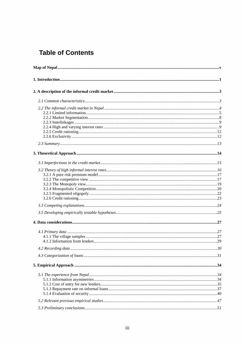
Table of Contents

Map of Nepal ............................................................................................................................................................v

1. Introduction..........................................................................................................................................................1

2. A description of the informal credit market ......................................................................................................3

2.1 Common characteristics..................................................................................................................................3 2.2 The informal credit market in Nepal ...............................................................................................................4

2.2.1 Limited information.................................................................................................................................5 2.2.2 Market Segmentation...............................................................................................................................8 2.2.3 Interlinkages ............................................................................................................................................9 2.2.4 High and varying interest rates ................................................................................................................9 2.2.5 Credit rationing......................................................................................................................................12 2.2.6 Exclusivity.............................................................................................................................................12

2.3 Summary........................................................................................................................................................13

3. Theoretical Approach ........................................................................................................................................14

3.1 Imperfections in the credit market.................................................................................................................15 3.2 Theory of high informal interest rates...........................................................................................................16

3.2.1 A pure risk premium model...................................................................................................................17 3.2.2 The competitive view ............................................................................................................................17 3.2.3 The Monopoly view...............................................................................................................................19 3.2.4 Monopolistic Competition.....................................................................................................................20 3.2.5 Fragmented oligopoly............................................................................................................................22 3.2.6 Credit rationing......................................................................................................................................23

3.3 Competing explanations ................................................................................................................................24 3.5 Developing empirically testable hypotheses..................................................................................................25

4. Data considerations............................................................................................................................................27

4.1 Primary data .................................................................................................................................................27 4.1.1 The village samples ...............................................................................................................................27 4.1.2 Information from lenders.......................................................................................................................29

4.2 Recording data ..............................................................................................................................................30 4.3 Categorization of loans .................................................................................................................................31

5. Empirical Approach ..........................................................................................................................................34

5.1 The experience from Nepal............................................................................................................................34 5.1.1 Information asymmetries .......................................................................................................................34 5.1.2 Cost of entry for new lenders.................................................................................................................35 5.1.3 Repayment rate on informal loans.........................................................................................................37 5.1.4 Evaluation of security............................................................................................................................40

5.2 Relevant previous empirical studies..............................................................................................................47 5.3 Preliminary conclusions................................................................................................................................51

iii

6. Conclusions.........................................................................................................................................................54

References...............................................................................................................................................................55

Appendix A: Questionnaire...................................................................................................................................57

Appendix B: Survey data results ..........................................................................................................................62

Stata commands: Chapter 2 ................................................................................................................................62 Stata commands: Chapter 5 ................................................................................................................................69

Appendix C: NLSS data results ............................................................................................................................70

iv

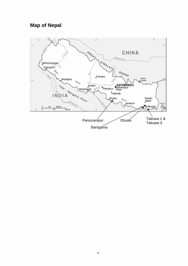
Map of Nepal

Parsurampur Dhuski Takuwa 1 & Takuwa 3

Banigama

v

vi

1. Introduction

Informal credit markets are still important in developing countries. Despite an increase in

supply of formal credit in rural areas, informal lenders remain the dominant source of credit

for the poorest households. Improvements in productivity are important in a development

process. Productive investment requires funding and the access to credit is crucial for this

purpose. Credit might also be a mean tide over bad times caused by sudden illness or an

upcoming wedding for poor individuals.

This thesis studies the informal credit market in Nepal. In 2004 Nepal was ranked as

number 140 out of 177 countries by the human development index (HDI) (Human

Development Report, 2004). In 2002 the gross domestic product (GDP) per capita was only

USD 1370. Nepal is one of the least developed countries in Asia.

Previous studies of the informal credit market demonstrate extremely high informal interest

rates charged on loans to poor individuals. Extensive rural credit programs the last decades

were intended to break the informal lenders anticipated monopoly power in the rural credit

markets. Competition was expected to lower the informal interest rates. However, these

policies do not seem to have improved the credit terms for the poorest households in rural

areas. In order to make policies that can positively affect poor people’s living conditions, we

must understand how informal lenders set the interest rates. There exist competing

explanations. One traditional explanation of high interest rates that opposes the monopoly

view, that has motivated credit programs in the past, is the Risk Premium hypothesis. This

theory argues that because there is a high share of default informal loans and lenders charge

a risk premium to cover loss due to default. This risk premium can explain the interest rate

gaps between formal and informal credit markets. We know about few previous studies of

repayment in South Asia, and none from Nepal. A main contribution of this paper is

therefore to provide data on default rates in Nepal. The data is based on field research

conducted over two months in Eastern Terai. We made 114 interviews in five sample

villages.

In chapter two we give a general description of informal credit markets in Nepal. Based on

data from five sample villages and the Nepal Living Standard Survey from 1996 we see that

1

the characteristics commonly used to describe the informal credit market are typical for the

informal credit markets in Nepal. We identify high and varying interest rates.

Chapter three presents theory that can explain high informal interest rates. (See e.g. Basu

(1993), Basu (1997), Ray (1998) and Hoff and Stiglitz (1993)) Since we are not testing

implications of a specific model, but rather focus on getting an overview of contemporary

theory, we find it adequate to present models in details, only when this is necessary to put

forward an important argument. Based on existing theory we outline three hypotheses that

are able to discriminate between different views of informal interest rate formation in

informal sector. They are: (1) The risk premium hypothesis (2) the searching cost

hypothesis (3) The monopoly rent hypothesis.

Before the empirical evaluation of survey data we find it necessary to present the method of

sampling and method used in the data processing. This is done under “data consideration” in

chapter 4.

In chapter 5 we evaluate the three different hypotheses empirically. Firstly, we present the

data and the findings from the village survey from Nepal. Secondly, we discuss how these

findings correspond to some previous empirical studies of informal interest rate formation.

(See e.g. Aleem (1993), Hatlebakk (2000) and Raj (1979))

Chapter 6 concludes.

2

2. A description of the informal credit market

The following chapter describes the credit market in Nepal. Based on our own field

experience and data from the Nepal Living Standard Survey (NLSS) from 1996 we discuss

whether characteristics commonly used to describe the informal credit market are typical for

Nepal.1

2.1 Common characteristics

Empirical studies of informal borrowing and lending in developing countries have resulted

in a list of common characteristics or “stylised facts” that is often used to describe informal

credit markets in poor countries. Raj (1998) specifies six such features:

1. Limited information: Lenders have, more often than not, limited information about the

borrower and how he spends the money.

2. Segmented markets: Relationships between borrowers and lenders are stable.

3. Interlinkages between markets: One often observes that interlinkages exist and the

outcome in one market affects the outcome in a different market.

4. High and varying interest rates: Interest rates are higher than the lenders’ opportunity

cost of lending and may vary within each village.

5. Credit rationing: Lenders that are often not able to lend more at the going interest rate,

but borrowers are willing to borrow more at the going interest rate.

6. Exclusivity: It is common that lenders refuse to lend to individuals that have

outstanding loans with other lenders.

1 The Nepal Living Standard Survey (NLSS) from 1996 follows the Living Standard Measurement Survey methodology developed by researcher at the World Bank during the last fifteen year and is applied in surveys conducted in more than thirty countries. The NLSS data consist of a household survey and a village survey. In the household survey a random sample of 3373 households where interviewed. Out of these, 744 households were from 62 different wards (villages) in the eastern part of the ecological belt of Terai, the region where the 5 villages we visited is situated. The Central Bureau of Statistics (CBS) has used the data from the household survey in the preparation of a two volume report. In this paper we refer to numbers from these reports, but also present some data from the original data set. See www.worldbank.org/lsms/country/nepal/nep96docs/html

3

Common for all these characteristics is that they are indicators of a credit market that diverts

from a perfectly competitive credit market. In this chapter we discuss whether these features

apply to the credit market in Nepal. Some of the features are more relevant for the analysis

in chapter 5 and will be elaborated further in this chapter.

2.2 The informal credit market in Nepal

A paper by Chowdury and Garcia (1993) reports that the supply of formal credit to rural

areas in Nepal increased from NR 806 million to NR 1480 million in the period between

1986 to 1990.2 A large share of this supply has been channelled through rural credit

programs. Despite an increased supply of formal credit, informal lenders are still the most

important source of credit among the poor in Nepal. Formal lending institutions often

require collateral like land from borrowers. The poorest households are often landless and

therefore excluded from formal credit programs. The NLSS reports show that only 16

percent of lending in rural Nepal is obtained from formal institutions. A relatively high

share of informal lending is also found in our samples; 60 out of 114 households have

informal loans and 95 households have formal and/or informal loans. When we asked

people why they do not borrower from formal institutions, the majority answered that they

were unable to do so because they do not owe land. Other reasons given for avoiding formal

credit are difficulties with illiteracy and high fees charged by officials.

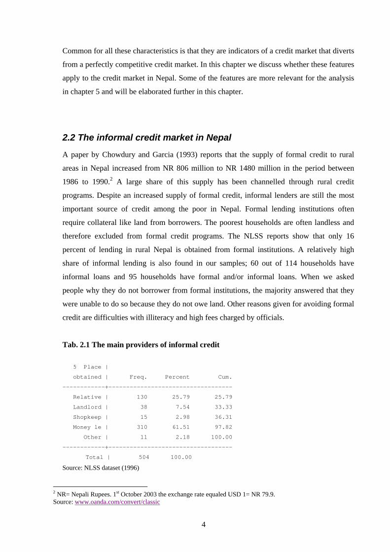
Tab. 2.1 The main providers of informal credit

5 Place |

obtained | Freq. Percent Cum.

------------+-----------------------------------

Relative | 130 25.79 25.79

Landlord | 38 7.54 33.33

Shopkeep | 15 2.98 36.31

Money le | 310 61.51 97.82

Other | 11 2.18 100.00

------------+-----------------------------------

Total | 504 100.00

Source: NLSS dataset (1996)

2 NR= Nepali Rupees. 1st October 2003 the exchange rate equaled USD 1= NR 79.9. Source: www.oanda.com/convert/classic

4

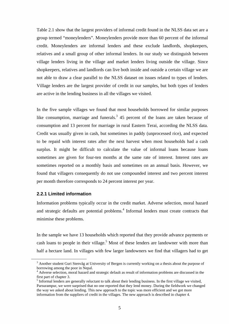
Table 2.1 show that the largest providers of informal credit found in the NLSS data set are a

group termed “moneylenders”. Moneylenders provide more than 60 percent of the informal

credit. Moneylenders are informal lenders and these exclude landlords, shopkeepers,

relatives and a small group of other informal lenders. In our study we distinguish between

village lenders living in the village and market lenders living outside the village. Since

shopkeepers, relatives and landlords can live both inside and outside a certain village we are

not able to draw a clear parallel to the NLSS dataset on issues related to types of lenders.

Village lenders are the largest provider of credit in our samples, but both types of lenders

are active in the lending business in all the villages we visited.

In the five sample villages we found that most households borrowed for similar purposes

like consumption, marriage and funerals.3 45 percent of the loans are taken because of

consumption and 13 percent for marriage in rural Eastern Terai, according the NLSS data.

Credit was usually given in cash, but sometimes in paddy (unprocessed rice), and expected

to be repaid with interest rates after the next harvest when most households had a cash

surplus. It might be difficult to calculate the value of informal loans because loans

sometimes are given for four-ten months at the same rate of interest. Interest rates are

sometimes reported on a monthly basis and sometimes on an annual basis. However, we

found that villagers consequently do not use compounded interest and two percent interest

per month therefore corresponds to 24 percent interest per year.

2.2.1 Limited information

Information problems typically occur in the credit market. Adverse selection, moral hazard

and strategic defaults are potential problems.4 Informal lenders must create contracts that

minimise these problems.

In the sample we have 13 households which reported that they provide advance payments or

cash loans to people in their village.5 Most of these lenders are landowner with more than

half a hectare land. In villages with few larger landowners we find that villagers had to get

3 Another student Guri Stenvåg at University of Bergen is currently working on a thesis about the purpose of borrowing among the poor in Nepal. 4 Adverse selection, moral hazard and strategic default as result of information problems are discussed in the first part of chapter 3. 5 Informal lenders are generally reluctant to talk about their lending business. In the first village we visited, Parsurampur, we were surprised that no one reported that they lend money. During the fieldwork we changed the way we asked about lending. This new approach to the topic was more efficient and we got more information from the suppliers of credit in the villages. The new approach is described in chapter 4.

5

loans from lenders outside the village, often in a nearby market area. Typical for lenders in

the village are that they only lend to certain people. “Aphno Manche” is best translated to

“our people” in English and is used by larger landowners and other more powerful people of

relatively high caste to describe a certain group of workers or neighbours that they have a

close relationship to. This relationship is often a work relationship, but also involves that the

landowner has some sort of responsibility for the individuals’ welfare and survival. The

expression can frequently be heard during an interview when we ask the landowners about

their lending activity. The landowners specify that loans are primarily given to “Aphno

Manche”, people they trust, and hence whom they know well. If they lend to people that are

not “their people”, the loans is often secured by a written contract. Villagers referred to a

contract as a “tamsuk”. We found that it is common practise to write a contract that states

the double, or as in one village, the triple of the loans sum. In the contract the interest rate is

only ten percent per year, whereas the actual interest rate is much higher. Written contracts

are more frequently used by market lenders to secure a loan and they give the lender the

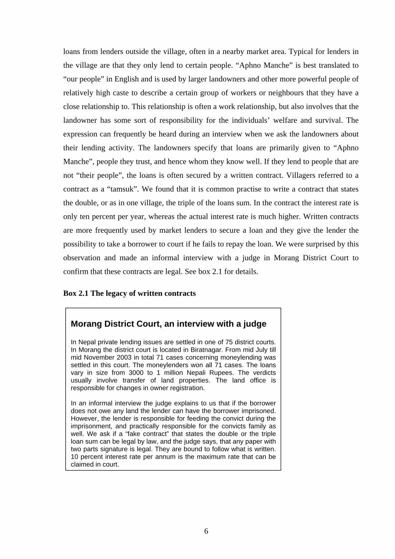
possibility to take a borrower to court if he fails to repay the loan. We were surprised by this

observation and made an informal interview with a judge in Morang District Court to

confirm that these contracts are legal. See box 2.1 for details.

Box 2.1 The legacy of written contracts

Morang District Court, an interview with a judge In Nepal private lending issues are settled in one of 75 district courts. In Morang the district court is located in Biratnagar. From mid July till mid November 2003 in total 71 cases concerning moneylending was settled in this court. The moneylenders won all 71 cases. The loans vary in size from 3000 to 1 million Nepali Rupees. The verdicts usually involve transfer of land properties. The land office is responsible for changes in owner registration. In an informal interview the judge explains to us that if the borrower does not owe any land the lender can have the borrower imprisoned. However, the lender is responsible for feeding the convict during the imprisonment, and practically responsible for the convicts family as well. We ask if a “fake contract” that states the double or the triple loan sum can be legal by law, and the judge says, that any paper with two parts signature is legal. They are bound to follow what is written. 10 percent interest rate per annum is the maximum rate that can be claimed in court.

6

In court we had the opportunity to study the record of court cases and count the number of

lending disputes settled in court over four months. We found that the number of court cases

is relatively low and that there would be only a small calculated risk of being prosecuted in

court because of a lending dispute. However, is interesting to see that a semi-formal credit

market exists in Nepal where informal lenders can formalize loans. In one village we were

told that lending cases were settled locally and that the Village District Community (VDC)

Committee or other well respected members of the community judge in lending disputes.

Villagers generally admit that they believe a lender will prosecute them if they default on a

loan.

The market lenders’ use of written contracts and the village lenders’ criteria for providing

loans indicate that there are information problems in these credit markets. However, the

village lenders are better informed about certain people and these therefore prefer to lend to

one of these. The market lenders that are not involved in any trade or other business in a

village are equally uninformed about all the potential borrowers in the village and have to

use other means to overcome the information problems like traditional screening methods,

collateral, written contracts or middlemen.

In one particular village, Takuwa 3, we find that one market lender who dominates the

credit market in this village use local and better informed middlemen to guarantee for a

borrower’s loan.6 These middlemen are trade partners or previous or current employees of

the moneylender and belong to his “Aphno Manche”. Personal guarantee is not a new

phenomenon and table 2.2, below, based on the NLSS illustrate that personal guarantee is

the most common type of security on informal loans.

In the NLSS survey, personal guarantee can be the signature of a well-established

businessman or landowner or witness of a good credit history.7 This involves that personal

guarantee will cover both written contracts and middlemen. The high share of personally

secured loans suggests that these are both common phenomenon in Nepal. Less than ten

percent of informal loans are secured with land. It may seem like a paradox that land is

important in order to obtain a loan, but that it is not important as security.

6A “ward” is often referred to as a village by the respondents themselves. For convenience we also prefer to refer to wards as villages. In most of the paper we talk about 5 villages, rather than 5 wards and 4 villages. 7 The interviewers’ manual pp. 86, see for a full version of the interviewers’ manual: www.worldbank.org/lsms/country/nepal/nep96docs/html

7

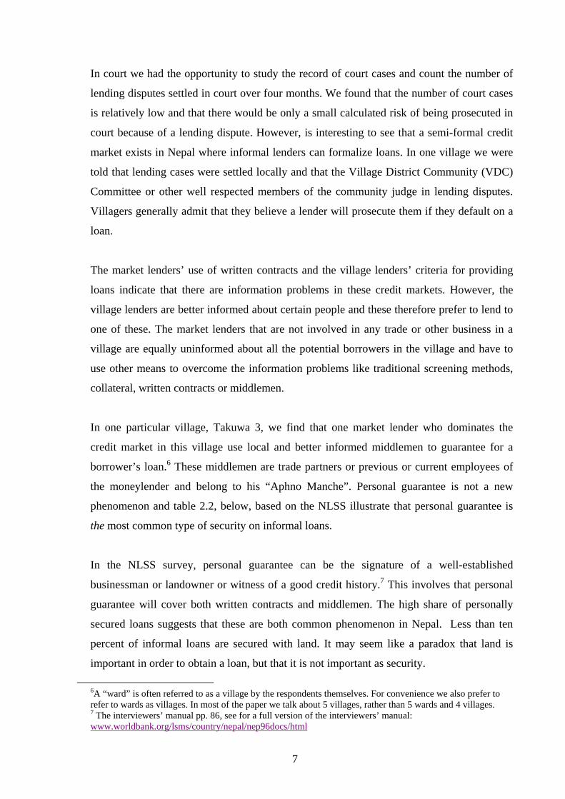
Tab. 2.2 Security reported on informal loans Kind of

collateral | Freq. Percent Cum.

------------+-----------------------------------

Agri. land | 43 8.51 8.51

Building | 10 1.98 10.50

Gold/silver | 15 2.97 13.47

Property | 10 1.98 15.45

Personal gua| 128 25.35 40.79

Other | 23 4.55 45.35

Nocollateral| 276 54.65 100.00

------------+-----------------------------------

Total | 505 100.00

Source: NLSS dataset (1996)

The NLSS reports show that in rural Eastern Terai 45 percent of the loans was secured by

some kind of collateral. The use of collateral indicates that there is a potential risk of default

that lenders attempt to reduce.

2.2.2 Market Segmentation

Market segmentation is a result of information problems. Village lenders seem to have well

defined groups of people that they consider themselves close to. This means that these

powerful landowners or lenders have specific preferences with regards to who they want to

deal with. This results in a segmented credit market as well as a segmented labour market.

Although our research showed that very few workers have permanent labour contracts in the

sample villages, we found that many have repeated work and credit relations with a specific

landlord or lender. In all the villages we visited we identified several segments within a

village. These segments where usually geographically defined.

In one village, Takuwa 1, we found that a group of low caste workers worked for less than

the average wage in the harvesting season. We asked them why they do not work for

someone else instead and earn better wages. The villagers said that they benefited from

remaining close to a certain landlord, living close by. Some stated that they were able to

work for the landlord in off-seasons, while others said they were able to let their cattle grass

on the landlord’s property. It was obvious that these stable relationships with landlords

where considered as a kind of insurance by this group of poor low caste people. In other

words stable relationships were necessary to obtain credit within the village.

8

2.2.3 Interlinkages

The discussion on market segmentation is closely related to interlinkages. In the

introduction we defined interlinkages as a situation where the outcome in one market affects

the outcome in another market. Such kinds of multiple relations are often found in informal

credit markets. In the sample villages from Nepal we saw that village lenders were

employers, shopkeepers, local paddy trades or mill owners. This involves that a lender

usually deals with a borrower in at least two different markets. In addition to the

informational advantage of knowing a potential borrower well, interlinkages give the lender

the opportunity to indirectly reclaim debt through another market transaction. The example

from Takuwa 1 where villagers work for less than the market wage can be an example of

interlinkages if parts of the wages are kept by the landlord as instalments on a loan. We also

hear stories of people that have worked for free in the off season to pay off debt. There are

possible advantages of an interlinked contract for both the borrower and the lender. The

lender can make the borrower work for lower wages and the borrower ensure a close tie to a

specific employer. Since interlinkages are not a main topic we did not get enough details on

interlinkages to examine this topic further.

2.2.4 High and varying interest rates

Table 2.3 below show that the average interest rate on informal loans in rural Eastern Terai,

is 40 percent per year. This is above the formal interest rate which at the time of our

research was 18 percent per annum on loans from ADB.

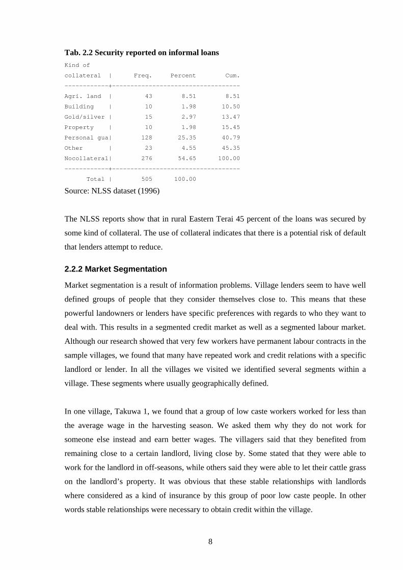
Tab. 2.3 The average interest rate and loan size in Eastern Terai

Variable Number of obs. Mean Std.Dev. Min MaxInterest rate 385 40 20 0 84Loansize 504 7695 13068 1000 150000

Source: NLSS dataset (1996)

The interest rates vary from zero to 84 percent. The zero percent interest loans are in 53

percent of the cases given by relatives and in 30 percent of the cases given by the group

moneylenders. Zero interest loans are interesting because they are loss contract. A lender

could be better off investing the money in alternative ways. We think that zero interest loans

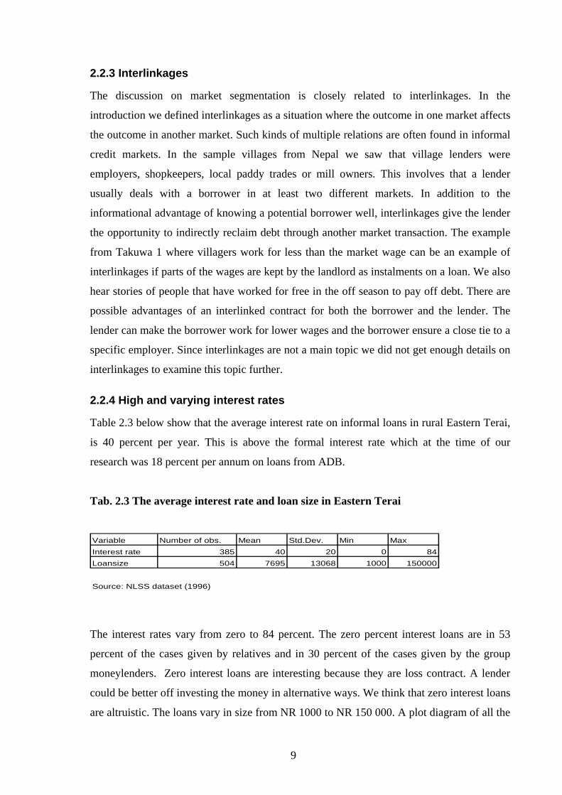
are altruistic. The loans vary in size from NR 1000 to NR 150 000. A plot diagram of all the

9

504 informal loans from rural Eastern Terai show that there is no obvious correlation

between interest rate and loan size found in the data (see fig. 2.1, below). The lack of

correlation is especially obvious for relatively small loans.

Fig. 2.1 Reported interest rates versus loan size

or

mar

kup o

n lo

an

(%

)

8 Amount borrowed (Rs)1000 150000

0

10

20

30

40

50

60

70

80

90

100

Source: NLSS dataset (1996)

In figure 2.1 there seems to be only a small tendency that interest rates increase with loan

size. The NLSS data shows that there is no clear difference between the interest rates

charged by different types of informal lenders either. The results are available as plot

diagrams in appendix C

In the five sample villages from Nepal we found that interest rates vary form zero percent to

120 percent per year. Table 2.4 present details from each village. Since villages are chosen

based on certain criteria we cannot immediately generalize the results. To keep the validity

of the data we keep the data on village level. We therefore consider the data valid only at

village level.8

8 The samples from each village are random, but the sample of villages are non random. The criteria for the choice of villages are presented in chapter four under the section on primary data.

10

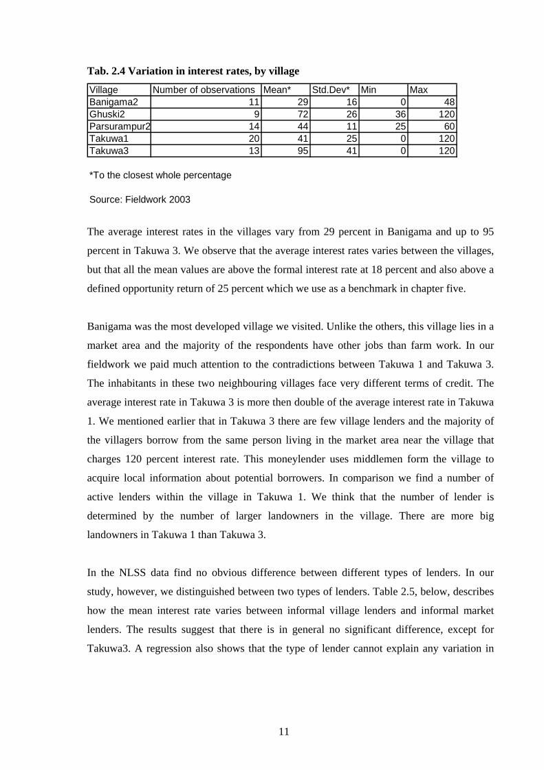
Tab. 2.4 Variation in interest rates, by village

Village Number of observations Mean* Std.Dev* Min MaxBanigama2 11 29 16 0 48Ghuski2 9 72 26 36 120Parsurampur2 14 44 11 25 60Takuwa1 20 41 25 0 120Takuwa3 13 95 41 0 120

*To the closest whole percentage

Source: Fieldwork 2003

The average interest rates in the villages vary from 29 percent in Banigama and up to 95

percent in Takuwa 3. We observe that the average interest rates varies between the villages,

but that all the mean values are above the formal interest rate at 18 percent and also above a

defined opportunity return of 25 percent which we use as a benchmark in chapter five.

Banigama was the most developed village we visited. Unlike the others, this village lies in a

market area and the majority of the respondents have other jobs than farm work. In our

fieldwork we paid much attention to the contradictions between Takuwa 1 and Takuwa 3.

The inhabitants in these two neighbouring villages face very different terms of credit. The

average interest rate in Takuwa 3 is more then double of the average interest rate in Takuwa

1. We mentioned earlier that in Takuwa 3 there are few village lenders and the majority of

the villagers borrow from the same person living in the market area near the village that

charges 120 percent interest rate. This moneylender uses middlemen form the village to

acquire local information about potential borrowers. In comparison we find a number of

active lenders within the village in Takuwa 1. We think that the number of lender is

determined by the number of larger landowners in the village. There are more big

landowners in Takuwa 1 than Takuwa 3.

In the NLSS data find no obvious difference between different types of lenders. In our

study, however, we distinguished between two types of lenders. Table 2.5, below, describes

how the mean interest rate varies between informal village lenders and informal market

lenders. The results suggest that there is in general no significant difference, except for

Takuwa3. A regression also shows that the type of lender cannot explain any variation in

11

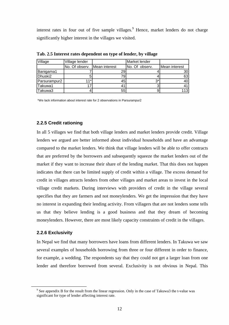
interest rates in four out of five sample villages.9 Hence, market lenders do not charge

significantly higher interest in the villages we visited.

Tab. 2.5 Interest rates dependent on type of lender, by village Village Village lender Market lender

No. Of observ. Mean interest No. Of observ. Mean interestBanigama1 7 29 4 30Dhuski2 5 79 4 63Parsurampur2 11* 45 3* 40Takuwa1 17 41 3 41Takuwa3 4 55 9 113

*We lack information about interest rate for 2 observations in Parsurampur2

2.2.5 Credit rationing

In all 5 villages we find that both village lenders and market lenders provide credit. Village

lenders we argued are better informed about individual households and have an advantage

compared to the market lenders. We think that village lenders will be able to offer contracts

that are preferred by the borrowers and subsequently squeeze the market lenders out of the

market if they want to increase their share of the lending market. That this does not happen

indicates that there can be limited supply of credit within a village. The excess demand for

credit in villages attracts lenders from other villages and market areas to invest in the local

village credit markets. During interviews with providers of credit in the village several

specifies that they are farmers and not moneylenders. We get the impression that they have

no interest in expanding their lending activity. From villagers that are not lenders some tells

us that they believe lending is a good business and that they dream of becoming

moneylenders. However, there are most likely capacity constraints of credit in the villages.

2.2.6 Exclusivity

In Nepal we find that many borrowers have loans from different lenders. In Takuwa we saw

several examples of households borrowing from three or four different in order to finance,

for example, a wedding. The respondents say that they could not get a larger loan from one

lender and therefore borrowed from several. Exclusivity is not obvious in Nepal. This

9 See appendix B for the result from the linear regression. Only in the case of Takuwa3 the t-value was significant for type of lender affecting interest rate.

12

observation also indicates that the market segmentation that we described above is not

perfect. There must be overlaps between the segments that different lenders operate within.

2.3 Summary

In this chapter we showed that many of the common characteristics of the informal credit

market are also typical for the informal credit market in Nepal. We identified high interest

rates in all the sample villages and large variation in interest rates both between and within

the villages. Information problems seem to be closely related to both the market

segmentation and the interlinkages that we observe. Since exclusivity is not obvious we

think that there are large overlaps between the segments. Important findings are that village

lenders and market lenders charges on average equally high interest rate and that there

does not seem to be a clear correlation between the size of a loan and the interest rates. The

use of middlemen and written contract as ways to reduce the information problems are

topics that we think are interesting and that got much attention during the fieldwork. These

topics are relevant in the discussion of security and liability in chapter 5.

13

3. Theoretical Approach

There are several theories that attempt to explain the characteristics of the informal credit

market outlined in the previous chapter. Standards economic theory assumes perfect

information, perfect contract enforcement and heterogeneous borrowers and lenders. Based

on these assumptions credit markets are modelled perfectly competitive, which results in

zero profit in equilibrium. Based on this model we should expect to observe one equilibrium

interest rate in one region reflecting the interception between demand and supply of credit in

the area. However, empirical studies of the credit market in developing countries

demonstrate the existence of a dual credit market and prove a gap between formal and

informal interest rates charged within the same region. Our field experience confirms these

findings. It is puzzling that such a set up does not cause arbitrage between the two sectors.

Why does our Homo economicus not take this opportunity to earn some easy money by

borrowing in the urban market and lending in the rural one?(Basu, 1997, pp.267)

Basu argues that if enough people saw this opportunity the informal interest rate would fall

and the formal interest would rise until equilibrium is restored. The fact that, this does not

happen, seems to render the standard competitive theory powerless when it comes to

explaining the high informal interest rates.

Attempts to find alternative explanations for the characteristics that we observe in the

informal credit market have resulted in a vast literature on the topic. Depending on the

approach, these theories emphasize different characteristics of the credit market, such as

interlinkages, market segmentation, high informal interest rates, credit rationing, risk and

information asymmetries. The ideal is to find a model that is able to capture as many of the

characteristics as possible. Typical for much of the new theories are that they are based on

more realistic assumptions about information and enforcement, than the classical

competitive theory. Imperfect information and enforcement problems are signs of market

imperfections and result in a potential risk of default and possibly monopoly power in the

informal credit market.

14

3.1 Imperfections in the credit market

The basics of lending are to provide a loan today and get it repaid, usually with an interest

rate, some time in the future. This natural time delay in a debt contract, as compared to an

instant exchange of two goods, makes lending potentially risky (Bardhan and Udry, 1999).

A credit contract involves a promise of future payments. Unless the provider of credit can

ensure that this promise is kept in the future, there will always be a risk that the promise is

not kept, and hence, repayment can fail. In formal credit markets in well-developed

countries these problems are largely overcome by strong legal enforcement in combination

with some kind of collateral and information databases where information about

individuals’ creditability is stored and equally available for all lenders. In developing

countries such devices are not readily available and formal lending institutions are usually

not willing to lend to poor individuals who are landless and with an unknown credit history.

In developing countries we observe that individuals that are unable to get loans from formal

institutions can still obtain credit from informal lenders. This indicates that informal lenders

are able to handle information- and enforcement problems.

In a credit market there are typically asymmetric information between a borrower and a

lender, where borrowers have full information about their productivity and their risk types,

but a lender lacks this information. This kind of information asymmetries may be captured

in a standard principal-agent model. When borrowers have private information about their

risk types, the lender is facing an adverse selection problem. Adverse selection is a pre-

contractual problem and we refer to this as the lenders screening problem later in the thesis.

If post-contractual action by the borrower is not verifiable for the lender, the problem is

called moral hazard. This problem can be thought of as a monitoring problem and we refer

to this as the incentive problem.

A third related issue concerning lending is the enforcement problem. This concerns the

borrower’s repayment decision. A lender must take actions to increase the likelihood of

repayment when repayment is possible and thereby avoid strategic default. When projects

fail and loans are defaulted on for unpredictable reasons like sudden illness, death and bad

weather conditions it is referred to as involuntary default. This means that even if a lender

15

has full information about a borrower there might be an enforcement problem, and a

potential loss, due to involuntary default.

We see that potential risk of default arise because of incomplete enforcement and

asymmetric information between borrowers and lenders. Informal lenders can reduce this

risk of lending by spending time and resources on screening and monitoring. All costs

associated with a reduction of this risk are referred to as searching costs. Costs associated

with default are termed risk premiums. Both searching costs and risk premiums adds to the

transaction costs of lending. It is useful to keep the searching costs and the risk premiums

separate, because risk premiums can be positive even when lenders have full information

about borrowers.

In a credit market there may exist, another kind of asymmetric information. If one lender is

better informed about a potential borrower’s creditability than another lender, or typically

has better access to this information, we may find that there is asymmetric information

between lenders in the credit market. This kind of information asymmetries possibly limit

the competition between lenders and enable the better informed lenders to act as

monopolists.

3.2 Theory of high informal interest rates

In this part we introduce theory that can explain high interest rates in informal credit

markets. To understand what causes high interest rates and how an interest rate gap sustains

between the formal and the informal sector in most developing countries we need to

understand how the informal lenders set the interest rates. Above we discussed how

information asymmetries and enforcement costs can adversely affect the credit market.

Different theories provide alternative explanations of high informal interest rates depending

on the assumptions made about information and enforcement problems. We present six

different approaches: Pure risk premium theory, a competitive view, a standard monopoly

outcome, a monopolistic competitive theory, theory of credit rationing and the theory of

fragmented oligopolies. We start by presenting three models that represent the two most

extreme predictions of interest rate formation; a perfectly competitive outcome and a

standard monopoly outcome. The other theories represent intermediate views.

16

3.2.1 A pure risk premium model

One traditional explanation to the high interest rates in informal sector is the Lender’s Risk

hypothesis (see e.g. Basu, 1997). The interest gap between the formal- and the informal

credit markets is explained by high default rates and a risk premium paid by the borrowers.

This theory describes a competitive credit market with possible information problems and

enforcement problems. There is no mechanism of risk reduction in the theory. This theory

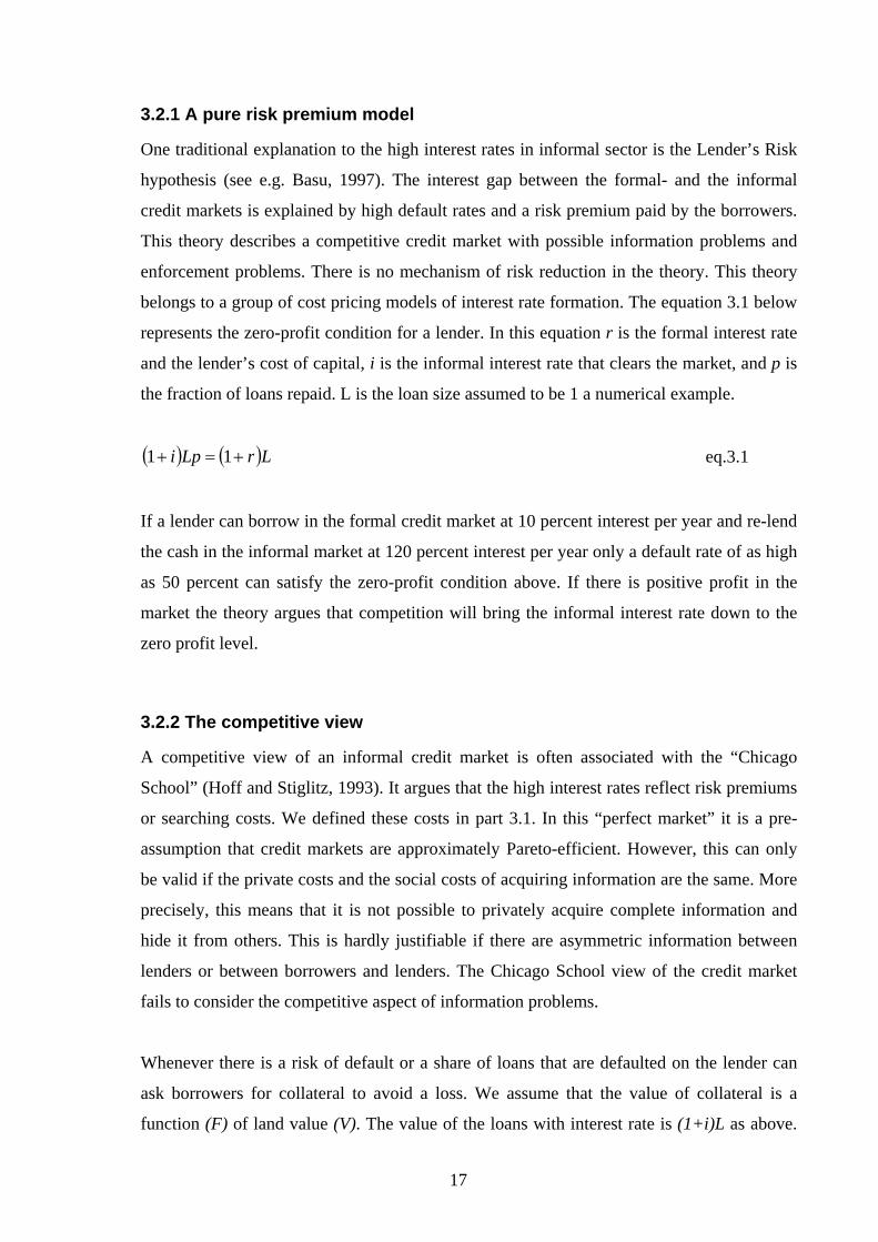
belongs to a group of cost pricing models of interest rate formation. The equation 3.1 below

represents the zero-profit condition for a lender. In this equation r is the formal interest rate

and the lender’s cost of capital, i is the informal interest rate that clears the market, and p is

the fraction of loans repaid. L is the loan size assumed to be 1 a numerical example.

( ) ( )LrLpi +=+ 11 eq.3.1

If a lender can borrow in the formal credit market at 10 percent interest per year and re-lend

the cash in the informal market at 120 percent interest per year only a default rate of as high

as 50 percent can satisfy the zero-profit condition above. If there is positive profit in the

market the theory argues that competition will bring the informal interest rate down to the

zero profit level.

3.2.2 The competitive view

A competitive view of an informal credit market is often associated with the “Chicago

School” (Hoff and Stiglitz, 1993). It argues that the high interest rates reflect risk premiums

or searching costs. We defined these costs in part 3.1. In this “perfect market” it is a pre-

assumption that credit markets are approximately Pareto-efficient. However, this can only

be valid if the private costs and the social costs of acquiring information are the same. More

precisely, this means that it is not possible to privately acquire complete information and

hide it from others. This is hardly justifiable if there are asymmetric information between

lenders or between borrowers and lenders. The Chicago School view of the credit market

fails to consider the competitive aspect of information problems.

Whenever there is a risk of default or a share of loans that are defaulted on the lender can

ask borrowers for collateral to avoid a loss. We assume that the value of collateral is a

function (F) of land value (V). The value of the loans with interest rate is (1+i)L as above.

17

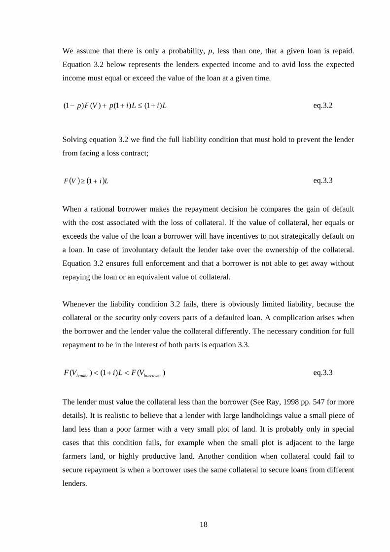
We assume that there is only a probability, p, less than one, that a given loan is repaid.

Equation 3.2 below represents the lenders expected income and to avid loss the expected

income must equal or exceed the value of the loan at a given time.

LiLipVFp )1()1()()1( +≤++− eq.3.2

Solving equation 3.2 we find the full liability condition that must hold to prevent the lender

from facing a loss contract;

( ) ( )LiVF +≥ 1 eq.3.3

When a rational borrower makes the repayment decision he compares the gain of default

with the cost associated with the loss of collateral. If the value of collateral, her equals or

exceeds the value of the loan a borrower will have incentives to not strategically default on

a loan. In case of involuntary default the lender take over the ownership of the collateral.

Equation 3.2 ensures full enforcement and that a borrower is not able to get away without

repaying the loan or an equivalent value of collateral.

Whenever the liability condition 3.2 fails, there is obviously limited liability, because the

collateral or the security only covers parts of a defaulted loan. A complication arises when

the borrower and the lender value the collateral differently. The necessary condition for full

repayment to be in the interest of both parts is equation 3.3.

)()1()( borrowerlender VFLiVF <+< eq.3.3

The lender must value the collateral less than the borrower (See Ray, 1998 pp. 547 for more

details). It is realistic to believe that a lender with large landholdings value a small piece of

land less than a poor farmer with a very small plot of land. It is probably only in special

cases that this condition fails, for example when the small plot is adjacent to the large

farmers land, or highly productive land. Another condition when collateral could fail to

secure repayment is when a borrower uses the same collateral to secure loans from different

lenders.

18

Collateral can explain how informal lenders might be able to solve information problems

and enforcement problems, but it is not obvious how this can be related to high interest

rates. If collateral is available to all lenders, at the same cost, and the use of collateral ensure

full liability, we would expect the informal credit market to be competitive. In that case this

full-liability theory can only explain high informal interest rates if there also are high

transaction costs involved in providing loans.

3.2.3 The Monopoly view

We introduce the other extreme of views on the informal interest rate formation. When

asymmetric information between moneylenders exists, we expect that some lenders have

advantages lending to certain people. This gives a lender market power in a segment of the

market where he is better informed than any competing lenders. When a lender is the single

best informed lender, or the only lender providing loans in the area, this lender is also likely

to have enforcement power. Even in the absence of collateral and threat of physical

punishment, a single lender can make sure that any borrower that defaults on a loan is

excluded from future credit. When the cost of exclusion is higher than the cost of

repayment, this threat will give the borrower incentives to not strategically default on a loan.

In a paper on informal insurance arrangements, Coate (1993) shows that repeated

interactions are efficient risk sharing arrangements in informal markets. This implies that a

borrower that is repeatedly dependent on credit to shed over bad tides will not default on

loans because of the treat of future exclusion from the market.

A single lender can use a pure monopoly strategy lending to people when there is no

information and enforcement problems. In a standard monopoly outcome the price, here the

interest rate, is higher than the competitive level and the monopolist is thus earning positive

profit.10

What happens if the monopolist is not able to overcome the enforcement problem? This

means that some loans are defaulted on. We examine the effect of default in a standard

monopoly model and identify two obvious effects. The simple result is based on the

assumption that default rate is independent of loans size. It might be more realistic to

10 Pure monopoly strategy: The moneylender offers a contract (i,L*), where the interest rate (i) charged is above the competitive level and the loansize (L) is rationed. The lender chooses L where marginal cost (MC) equals marginal revenue (MR). The interest is determined by the borrowers demand for credit (See e.e. Varian (1999), Intermediate microeconomics, pp. 423 figure 24.5).

19

assume that larger loans are more likely to become defaults. However, in this model we

keep things as simple as possible.

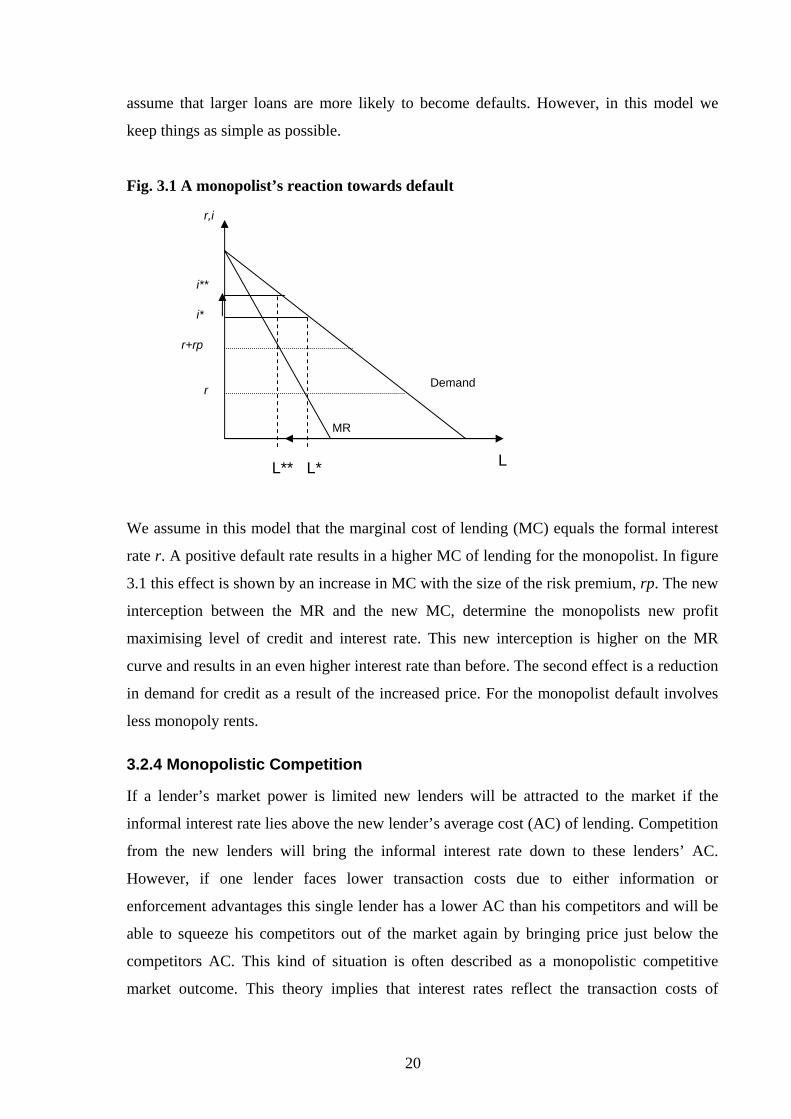
Fig. 3.1 A monopolist’s reaction towards default

r,i

i**

i*

r+rp

Demand r

MR

L L** L*

We assume in this model that the marginal cost of lending (MC) equals the formal interest

rate r. A positive default rate results in a higher MC of lending for the monopolist. In figure

3.1 this effect is shown by an increase in MC with the size of the risk premium, rp. The new

interception between the MR and the new MC, determine the monopolists new profit

maximising level of credit and interest rate. This new interception is higher on the MR

curve and results in an even higher interest rate than before. The second effect is a reduction

in demand for credit as a result of the increased price. For the monopolist default involves

less monopoly rents.

3.2.4 Monopolistic Competition

If a lender’s market power is limited new lenders will be attracted to the market if the

informal interest rate lies above the new lender’s average cost (AC) of lending. Competition

from the new lenders will bring the informal interest rate down to these lenders’ AC.

However, if one lender faces lower transaction costs due to either information or

enforcement advantages this single lender has a lower AC than his competitors and will be

able to squeeze his competitors out of the market again by bringing price just below the

competitors AC. This kind of situation is often described as a monopolistic competitive

market outcome. This theory implies that interest rates reflect the transaction costs of

20

lending. In equilibrium the interest charged will be lower than in a pure monopoly. The

lender with information and enforcement advantages can still earn some profit in

equilibrium. The competitors, on the other hand, are willing to stay in the market until their

rofits are zero. This theory has been presented in Bardhan and Udry (1999).

formation in a model of monopolistic competition where enforcement costs are

ecified.

reason, then the

quilibrium interest rate charged will increase. (Hoff and Stiglitz, 1997)

credit market. Nevertheless, the model is useful in the discussion of interest rate

rmation.

of

riable costs. This is further supported by the empirical-based study by Aleem (1993).11

p

Next we describe a model used by Hoff and Stiglitz (1997) in some details to investigate the

interest rate

sp

A moneylender, once he has screened an individual and assessed the likelihood of

repayment, is an imperfect substitute for any other moneylender. Therefore, if there is free

entry into money lending, the market is appropriately modelled as monopolistically

competitive. If the marginal cost of money lending rises for some

e

In this model the authors argue that problems of enforcing contracts are common in

developing countries, but that there seems to be relatively free entry into the market,

although some lenders have advantages enforcing debt contracts. The authors claim that a

monopolistic competitive model can best describe features of the informal credit market.

The model should originally shed lights on the effect of increased formal subsidized credit

in the rural

fo

The equilibrium condition is characterized by two conditions: Zero-profit implying average

cost (AC) per unit lent equals the interest rate, and profit maximization implying that the

elasticity of the average cost curve equals the elasticity of the demand curve. The latter

condition ensures tangency between the AC and the demand curve. It is assumed that the

demand curve is downward sloping and that the AC curve is U-shaped. The U-shaped AC

curve reflects the view of the authors; that scale economies operates strongly at the level

va

11 More on Aleem (1990) in chapter 5.

21

Aleem (1993) presents a “Chamberlian theory” of a monopolistically competitive credit

market based on a study of 14 market lenders in the Chamber region in Pakistan. He finds

that an increase in default, or an increase in marginal cost of funds, e.g. the formal interest

rate, increases the interest rate. This last statement regarding the positive correlation

between formal interest and marginal cost of lending is reversed by Hoff and Stiglitz who

argue that an increase in the subsidised funding will decrease the opportunity cost of funds,

but lead to an increase in marginal costs of lending. More and cheaper credit available for

moneylenders is likely to attract new lenders and increase marginal cost. The authors model

three different situations where this might be true. We briefly describe the argument

intuitively: (1) New entry reduces each lender’s share of the market and forces him to

operate at a higher marginal cost.12 (2) New entry gives a borrower more choices, then

adversely affects it’s incentives to repay. This increases the marginal cost of the lender

through higher default or higher enforcement costs. (3) New entry weakens the information

sharing among lenders, and reduces the effect of reputation that at a smaller scale can have a

positive incentive effect on the borrower. High interest rates in this model are explained by

transaction costs. An increase in formal subsidies causes an even higher informal interest

rate.

3.2.5 Fragmented oligopoly

A different approach to model the informal credit markets has been to assume that two

lenders act as monopolists in respectively segment, ( )1S and ( )2S , then competes in a third

segment, ( )3S This market simulation gives another outcome, considerable more complex

than the monopolistic competitive outcomes mentioned earlier. An attempt to model such a

fragmented market has been presented in Basu (1997). A fragmented market can neither be

modelled as several standard monopolies nor a standard oligopoly.13 To model a fragmented

oligopoly, Basu argued, seems to be a closer verge on reality. Basu’s model can be used to

analyze the interest rate formation in fragmented markets. When the price function is

concave Basu proves that equilibrium interest rate charged will be less than a monopoly, but

higher than in an oligopoly. A similar idea is described in Basu and Bell (1991) and

Hatlebakk (2000). Hatlebakk tested this outcome on cross sectional household data from

Nepal. He finds that the model is useful in explaining high interest rates in the rural credit

12 See fig. 2 in Hoff and Stiglitz (1997) 13 Standard Oligopoly: In a oligopoly a lender is maximising profit, taking into consideration, a second lender’s actions. The result is a interest rate above the competitive, but below the monopolistic interest rate.

22

market where default rates are relatively low.14 His model predicts that in villages with low

lending capacities the interest rates are determined by the demand for credit and lenders can

earn positive profit. This means that high interest rates in a capacity constraint village might

not correspond to transaction costs. In villages with higher lending capacities one can expect

interest rates to proceed towards a competitive level. Hatlebakk also looks into the

possibility of price collision in village with high lending capacities (See. Hatlebakk (2000)

odel can also explain variation in interest rate between villages.

enders

ill not raise the interest in order to induce a riskier group of clients. This model originally

er interest rates

order to steal another lender’s customer. This might seem like a contradiction to the

by an equally low interest rate when the customer being

ompeted for is “good” credit risk and will not be matched if the borrower is not a

ument depends on the assumption that the lenders know who their most

figure 1 for details). This m

3.2.6 Credit rationing

Stiglitz and Weiss (1981) developed a model of credit rationing in a formal credit market.

This model is also useful in a study of the informal credit market. The authors assume that

lenders are have limited monopoly power. They assume that a borrowers willingness to pay

high interest rates reflect a borrower’s risk type. This positive relation between risk of

default and interest rate give lenders incentive to ration credit. In equilibrium Stiglitz and

Weiss argue that there might be borrowers that are willing to pay an even higher interest

rate than the market rate. However, because these are all high risk borrowers the l

w

argues that informal interest rates might be lower than the equilibrium interest rates.

In a competitive aspect, the model can also explain high interest rates. Because of the

relationship between risk and interest rates the lenders lack incentives to low

in

previous arguments, but Stiglitz and Weiss explains it in the following way:

If a bank tries to attract the customers of its competitors by offering a lower interest rate, it

will find that its offer is countered

c

profitable customer of the bank.15

This arg

creditworthy customers are. Interest rates can reflect both costs and monopoly rent in this

model.

14 A report of “low default” from this thesis would strengthen Hatlebakk’s conclusions. 15 Stiglitz and weiss (1981), “Credit rationing” in The American Economic Review, Vol. 71, No.3, page 409

23

Another example of credit rationing has been modelled by Bell (1990). He models the

interactions between formal and informal credit institutions. This model shows that when

formal credit is rationed, and the informal lender is able to offer a contract (L,i) that are

preferred by the borrower, there is a spill-over of demand in the market. This means that if

formal institutions do not do not give as much credit as a borrower desires the borrowers

will turn to informal lenders. Bell has data from Punjab in India that supports this

conclusion. Bell shows that the informal interest rate in equilibrium might be higher than

the formal interest rates, depending on the default rate and the cost of entry for new

moneylenders and hence the level of competition. The model is of particular interest

ecause it is a unified model that can be used to analyse several special cases, both of the

cost pricing hypothesis and the monopoly theory. This dichotomy is the main focus as we

s. These

we observe high and varying interest rates in informal credit markets:

) High interest rates are mainly due to high transaction costs. Implicit in this explanation

he basic idea is that in equilibrium the difference between the informal interest rate (i) and

the commercial inte

risk-premium (rp).

b

proceed.

3.3 Competing explanations

The three factors transaction costs, risk and market power are typical for theory that can

explain the interest rate formation in informal credit markets in developing countrie

are factors that make it inappropriate to use the standard competitive model to describe

these markets. We can depart from the competitive model in two directions that each may

explain why

a) High interest rates are mainly due to monopoly rents. Moneylenders have monopoly

power in a segment of the market and can charge interest above marginal cost of credit on

their loans.

b

will be that money lending is a relatively competitive business where the interest rate

reflects searching costs and/or a risk premium.

T

rest rate (r) is explained by searching costs (sc), monopoly rent (mp) or

a

rpmpscri ++=− eq. 3.4

24

Equation 3.4 indicates that the high interest rate can be explained by a single factor or by a

combination of two or all three of the factors in the equation. To determine whether risk

erest formation in Nepal

efault rate can also be an indicator of

mited market power. The monopolistic competitive theory suggests that if new lenders can

competitors’

verage cost of lending without facing competition. Monopoly rents are also possible in

illages that are characterized by capacity constraints.

s observed in the informal lending market this implies that risk

remiums cannot explain high informal interest rates. Contrary, if there is a positive default

efault and risk premiums affect the informal interest rate

necessary condition for a searching cost hypothesis is information and/or enforcement

pend time and resources on solving the screening-,

premiums, searching costs or monopoly power dominate in the int

we need to find ways to empirically discriminate between these competing views.

3.5 Developing empirically testable hypotheses

The theory that we have presented in this chapter suggest that how high informal interest

rates are set, depends on the level of competition and the possibilities for lenders to earn

monopoly rent in the informal sector. A competitive credit market is characterized by free

entry. The high interest rates reflect transaction costs. In this case the interest rate gap

between the rural and the urban sector is explained by searching costs, enforcement costs or

a risk premium. Variations in interest rates across villages are due to variations in lending

costs between these villages. Put differently, if a lender faces no competition the interest

rates may reflect monopoly rent. When a monopolist faces a positive rate of default, this

may result in an even higher interest rate. A positive d

li

enter the market at some cost, no lender can charge interest rates above the

a

v

We present the three following hypotheses concerning interest rate formation;

(1) The risk premium hypothesis

If there are no default

p

rate we cannot ignore that risk of d

formation. A necessary condition for the risk premium hypothesis is a positive rate of

default in equilibrium.

(2) A searching cost hypothesis

A

problems. When informal lenders s

25

monitoring- and enforcement problems, then there are searching costs involved in lending,

and we cannot reject the searching hypothesis.

(3) The monopoly rent hypothesis

If there is one single lender operating in a market or a segment of the market, this lender is a

potential monopolist and high interest rates can therefore reflect monopoly rent. If there are

two or more lenders in the market and these do not cooperate the hypothesis is rejected and

e interest rate can only reflect the cost of lending and the market is thus monopolistically

necessary condition for monopoly rent is cost of entry or

apacity constraints.

In the following we draw on data from the field experience to test the relative explanatory

power of these three hypotheses.

th

competitive. However, the latter is only viable if the interest rate reflects the sum of risk

premium and searching costs. A

c

26

4. Data considerations

The empirical evaluations in chapter five are essentially based on knowledge obtained from

a primary data source. This chapter describes the sampling method and discusses briefly the

quality of the survey data. In order to determine a default rate on loans in the sample we

classify loans in seven categories according to the likelihood that they are loss contracts.

The specific criteria we use for each category are summarized in a separate section below.

4.1 Primary data

The survey data were the collected over two months in the Eastern Terai of Nepal during the

autumn of 2003. Because of the ongoing conflict between the government and the Maoist

oppositions we found that we had to be especially careful. We decided to stay in bigger

cities instead of smaller market areas and do day trips to the villages. This geographically

limited the areas where we were able to do research.

4.1.1 The village samples

We did in total 114 interviews in five villages. The villages were chosen on the basis of

certain criteria. Since the fieldwork lasted only about 2 months, we wanted to visit villages

that were of particular interest given our research topic. Using the NLSS survey we

identified villages in Eastern Terai, with respectively low wages, high informal interest rate

and low caste groups that we felt were of interest.16 The non random choice of villages

implies that the results cannot immediately be generalized to represent all villages in the

region where we did research.

The sample of individuals from each village was randomly chosen from the most recent

voters’ list available. This implies that data must be considered valid at village level. Details

on the random samples can be found in table 4.1. We obtained information through personal

16 To single out the villages in question, we list the villages that fit the following two criteria: 1) There are at least 10 workers in the sample that are in the group of muslims, sarki or the combined category of other ethic groups. The data show that these groups earn the lowest wages. 2) The villages have an average unweighted wage of less than NR 34. Among the villages with these criteria we chose to visit villages that could be accessed by car and that lied close to an urban area, where we felt it was safer to stay because of the security situation in Nepal at the time of the fieldwork. In addition we look at the interest rate that should be above 25 percent.

27

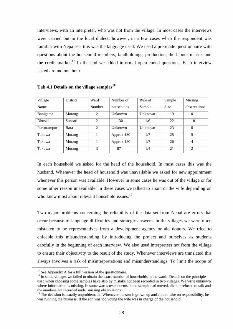
interviews, with an interpreter, who was not from the village. In most cases the interviews

were carried out in the local dialect, however, in a few cases when the respondent was

familiar with Nepalese, this was the language used. We used a pre made questionnaire with

questions about the household members, landholdings, production, the labour market and

the credit market.17 In the end we added informal open-ended questions. Each interview

lasted around one hour.

Tab.4.1 Details on the village samples18

Village

Name

District

Ward

Number

Number of

households

Rule of

Sample

Sample

Size

Missing

observations

Banigama Morang 2 Unknown Unknown 19 0

Dhuski Sunsari 2 130 1/6 22 10

Parsurampur Bara 2 Unknown Unknown 23 0

Takuwa Morang 1 Approx 180 1/7 25 5

Takuwa Morang 1 Approx 180 1/7 26 4

Takuwa Morang 3 87 1/4 21 2

In each household we asked for the head of the household. In most cases this was the

husband. Whenever the head of household was unavailable we asked for new appointment

whenever this person was available. However in some cases he was out of the village or for

some other reason unavailable. In these cases we talked to a son or the wife depending on

who knew most about relevant household issues.19

Two major problems concerning the reliability of the data set from Nepal are errors that

occur because of language difficulties and strategic answers. In the villages we were often

mistaken to be representatives from a development agency or aid donors. We tried to

enfeeble this misunderstanding by introducing the project and ourselves as students

carefully in the beginning of each interview. We also used interpreters not from the village

to ensure their objectivity to the result of the study. Whenever interviews are translated this

always involves a risk of misinterpretations and misunderstandings. To limit the scope of

17 See Appendix A for a full version of the questionnaire. 18 In some villages we failed to obtain the exact number of households in the ward. Details on the principle used when choosing some samples have also by mistake not been recorded in two villages. We write unknown where information is missing. In some wards respondents in the sample had moved, died or refused to talk and the numbers are recorded under missing observations. 19 The decision is usually unproblematic. Whenever the son is grown up and able to take on responsibility, he was running the business. If the son was too young the wife was in charge of the household.

28

language problems we used field assistants that were familiar with the local dialect of

Nepali in the region where we conducted the research. We also rehearsed the interview

process before doing interviews in the villages to make sure that the field assistants were

familiar with the questionnaire.

4.1.2 Information from lenders

In addition to the sample, we made a number of extra interviews with moneylenders. We

experienced that lenders are generally reluctant to talk about their lending business. Much of

the information we have about the lending activities in rural areas of developing countries

are based on information from the demand side of the credit market. Interest rate, loan size,

collateral and even repayment are easy to obtain information on by asking the borrowers.

However, when seeking information on screening, risk evaluation or for example indirect

payments the lenders are likely to be better informed than the borrowers.

In the first village we visited no one reports being involved in lending activities. We were

puzzled by this and assumed that something was wrong with the approach that we had to the

topic. When interviewing potential lenders in the second village we did not ask directly

whether someone was lending money. Instead we kept asking about borrowing. The idea is

pretty straight forward. We ask about any formal or informal borrowing and where they get

loans. When land is available, it is easier to obtain loans. The next step was to ask what

possibilities there are to borrow money if one lacks assets like land. This is the crux of the

strategy. Most respondents said that they had to turn to landlords or employers, relatives or

neighbors. If the respondent earlier had reported being an employer of landlord- we

followed up with whether his employees or peasants ever asked for credit. With this

approach it became difficult for the potential lenders to not admit actual lending. However,

we have to accept that some lenders were unwilling to go into any details on the matter.

This method works well because as long as the respondent lacks information about the

interviewer’s knowledge and intention of asking a specific question, the respondent will not

have incentives to avoid honesty. Therefore as long as we can “hide” that we are well

informed about the role and behaviour of lenders in rural credit markets and do not give the

lender a suspicion of the direction of the next question, we may get answers to some of the

questions we are interested in. Other advantages with this method, other than the

informational aspect, are that the conversation can be kept rather informal, although

29

structured, and that it gives us a more polite and less abrupt way to approach a sensitive

topic.

4.2 Recording data

All answers are registered in the questionnaire and later put into a MS Excel worksheet. The

working sheet is later transferred to Stata for analysis. To make the data more

comprehensible we had to make some critical decision about how we transfer detailed data

from the questionnaires into the Excel working sheet. We summarize the assumptions that

we find questionable below.

• Loan size: If the loan was taken in paddy (unprocessed rice), the value of the loan is

written in this column. The price of paddy varied with seasons and the price was

lower during the harvest time when it is readily available. In Parsurampur the price

of 1 Mon (20Kg) paddy was NR 200 after the harvest and NR 400 in other seasons.

In Banigama the price varied from NR 250 to NR 400. Similar variations were found

in the rest of the villages. As a common average we assumed that the value of 1 Mon

(20Kg) paddy equals NR 300 whenever a loan was taken in paddy.

• Land: Land was reported in local measures of Dur, Khatta and Bigha.20

• Lender: We define two categories of lenders; v (village) and m (market) dependent

on whether the lenders were resident in the village or from other villages or a market

area. Credit providers from other villages were recorded as market lenders.

• Security: We register six kinds of security as dummy variables in the working sheet.

The list below gives the definitions of each of these variables.

1. Mortgage: Mortgage means that as long as a loan is outstanding the lender is

entitled to use of a plot of land.

2. Land/gold: Land was only assumed to be available as collateral when the

respondents reported that they have more than 2 Khatta land, or owed some

agricultural land in addition to house land. By using “no land” as benchmark

we expected a larger error in the data because we noticed that some

respondents reported no land when possessing only house land, while others

reported positive landholdings.

20 20x20 Dur= 20 Khatta= 1 Bigha= 0.6773 Hectare, Statistical Pocket Book 2002, CBS, Katmandu, Nepal

30

3. Repeated loans: Whenever a borrower reported that he had previously

borrowed from the current lender we recorded repeated lending.

4. Remittance: If a borrower owed cattle or had sources of income other than

farm work above or equal to NR 1000 a month, this is recorded as

remittance. Farm work in Punjab and permanent labour work were typical

examples of this. The data on herds are not very good.

5. Paper: Whenever a contract was signed as a proof of the credit relationship is

was registered.

4.3 Categorization of loans

In order to determine default rates on informal loans in the sample villages we have to

divide data into different categories. We find it natural to classify loans as potential defaults,

as defaults on contracts, or as recent and unclassifiable loans. Important determinants, of

which category that each loan falls in, are age of the loan and the amount repaid. After all

loans have been categorized we choose one loans to represent each household. Households

with more than one informal loan we choose the loan that fall in the lowest category and

hence, are most likely to be a default.

All individual loans can be put in one of the seven categories that we define in table 4.2,

below. We make two crucial assumptions: (1) Loans less than NR 1000 are considered

unclassifiable. Loans less than NR 1000 are usually short term shop credit or advance

payments on wages. We assume that households that have borrowed less than NR 1000 are

not indebted and hence there is no risk of default on these loans. (2) The opportunity cost of

funds is assumed to be 25 percent per year. This is higher than the marginal cost of funds

which was 18 percent on loans from the ADB bank at the time of research. We assume that

in these less developed regions with relatively cheap and readily available labour capital the

expected return from investing money in businesses other than lending will yield a high

return. In a study of money lending in Pakistan, the researcher calculated the opportunity

cost of funds and found that this was on average 23 percent per year (see Aleem, 1993). 25

percent is assumed to be the opportunity cost of funds in this thesis. The inflation rate in

Nepal at the time was less than five percent (Central Bureau of Statistics, Kathmandu, Nepal

2002).

31

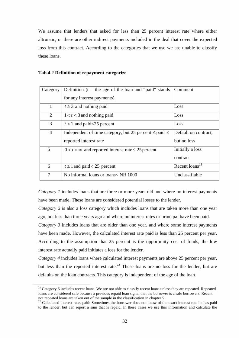
We assume that lenders that asked for less than 25 percent interest rate where either

altruistic, or there are other indirect payments included in the deal that cover the expected

loss from this contract. According to the categories that we use we are unable to classify

these loans.

Tab.4.2 Definition of repayment categorize

Category Definition (t = the age of the loan and “paid” stands

for any interest payments)

Comment

1 3≥t and nothing paid Loss

2 31 << t and nothing paid Loss

3 1>t and paid<25 percent Loss

4 Independent of time category, but 25 percent ≤paid ≤

reported interest rate

Default on contract,

but no loss

5 ∞<< t0 and reported interest rate 25≤ percent Initially a loss

contract

6 1≤t and paid percent 25< Recent loans21

7 No informal loans or loans< NR 1000 Unclassifiable

Category 1 includes loans that are three or more years old and where no interest payments

have been made. These loans are considered potential losses to the lender.

Category 2 is also a loss category which includes loans that are taken more than one year

ago, but less than three years ago and where no interest rates or principal have been paid.

Category 3 includes loans that are older than one year, and where some interest payments

have been made. However, the calculated interest rate paid is less than 25 percent per year.

According to the assumption that 25 percent is the opportunity cost of funds, the low

interest rate actually paid initiates a loss for the lender.

Category 4 includes loans where calculated interest payments are above 25 percent per year,

but less than the reported interest rate.22 These loans are no loss for the lender, but are

defaults on the loan contracts. This category is independent of the age of the loan.

21 Category 6 includes recent loans. We are not able to classify recent loans unless they are repeated. Repeated loans are considered safe because a previous repaid loan signal that the borrower is a safe borrowers. Recent not repeated loans are taken out of the sample in the classification in chapter 5. 22 Calculated interest rates paid: Sometimes the borrower does not know of the exact interest rate he has paid to the lender, but can report a sum that is repaid. In these cases we use this information and calculate the

32

Category 5 includes loans where the reported interest rate is less than 25 percent. These

loans are according to the assumption about the opportunity cost of funds, assumed to be

initial loss contracts and we are not able to classify these loans.

Category 6 includes loans that are taken within the last year and where interest rates below

25 percent are already paid.

Category 7 is a sum category where households with no informal loan or only informal

loans below NR 1000 are recorded.

We choose one loan for each household. If a household has more than one informal loan

above NR 1000 we choose the loan that falls in the lowest of the categories, (1-6)23. If the

respondent has two or more loans in the same category we use the following determinants in

the respective order to rank the risk of the loans:

a) Oldest

b) Biggest

c) Highest interest

The argument is that the older the loan, the more likely the loan is to be a default. Secondly,

the size of the loan matter because it is likely to affect the incentives to default. The bigger a

loan is, the larger is the gain from default. Thirdly, when a borrower fails to pay interest rate

we expect the value of the loan to increase. When the interest rate is high, the size of a loan

can grow so big that it is unrealistic that a borrower is able to repay the outstanding loan.

interest rate paid. Calculated interest paid (c) is defined by equation 4.1. Variable list: Interest payment (I), Principal (K), and Time (t), yearly or monthly;

t

xKIc 100

=

When nothing is paid on the loan the calculated interest is zero. Whenever c is above 25 the lender is recoverable enough to cover the opportunity costs of lending. The definition of c is a simple formula that ignores any compounded interests. During the fieldwork we found that compounded interest is usually not added to the value of the loan. It seemed more appropriate to use this kind of simple formula to calculate c. There will also be an inaccuracy due to little detailed information about when any amount was paid. Our method will overestimate the individual’s payment.

23 Loans in category 7 are unclassifiable and will not be evaluated.

33

5. Empirical Approach

In this chapter we evaluate the hypotheses outlined in chapter 3 empirically. By discussing

information asymmetries, cost of entry and repayment rates we conclude whether we find

support for any of the three hypotheses about searching costs, monopoly rents and risk

premiums or whether any of the three hypotheses are rejected.

After looking at data from Nepal in 5.1 we relate our study to some previous empirical

studies of informal interest rate formation in 5.2. Aleem (1993), Hatlebakk (2000) and Raj

(1979) have all studied empirical data and made conclusions on how informal lenders set

their interest rates. We shall see that our analyses in some ways both confirm and contradict

the results reported in the studies mentioned above. Part 5.3 concludes.

5.1 The experience from Nepal

During the fieldwork we focused on getting detailed data on repayment. We examine the

repayment data using the methods described in chapter 4. The information we gathered

enable us to give a brief discussion of the costs and information asymmetries.

5.1.1 Information asymmetries

In Nepal we found that village lenders only lend to people they refer to as “their people”

which means individuals whom they know well. This indicates that village lenders know a

potential borrowers risk types and we assume that screening problems for village lenders are

largely solved by personalized relationships and interlinkages between markets. We suppose

that village lenders do not face any significant screening costs. Both village and market

lenders were active in all villages we visited. Market lenders who are not involved in local

trade or village activities lack first hand information about potential borrowers’ credibility.

These lenders solve the screening problem by for example using local middlemen,

traditional screening methods or written contracts.24 Traditional screening methods can be

24 The screening process is described in details in Aleem (1993): The typical screening process involved getting information from about a loan applicants credit history from a third person whom know both the loan applicant and the lender. In addition, new loan applicants are usually given a small “test loans” the first time they get credit. Only if this loan is repaid, and the borrower satisfies the lender’s requirements the applicant is accepted and can rely on this lender for credit. A screening process usually takes about a year.

34

time consuming and is a costly way for a market lender to solve information asymmetries.

We found that imperfectly informed lenders preferred to use written contracts to overcome

information problems and ensure full liability. Enforcing these contracts in court involves a

court fee and is costly.

Under the section on market failure in chapter 3 we said that information asymmetries

between borrowers and lenders also cause an incentive problem. The village lenders we

talked to said that they kept a close eye on their loan customers. However, it is

problematical to estimate any cost of these actions based on our data. Since village lenders

live close to the borrowers and have multiple relations with them it is difficult to say

whether monitoring a loan customer involves extra time and effort.

In one village we found that a less informed market lender used middlemen. This implies

that the lenders solve the information asymmetries by using a local and better informed

middleman to guarantee for the person that ultimately got the loans. This middleman

belongs to the market lender’s “Aphno Manche” and is someone that the moneylender

knows well and trusts. We can not exclude the possibility that the market lender must

monitor the middleman and that this involves some extra costs. If this is the case there is a

double incentive problem involved in these credit arrangements where the market lender

must monitor the middleman and the middleman must monitor the borrower. Any searching

costs involved in making the contract are therefore likely to be shared between the market

lender and the middlemen. We cannot reject that there are transaction costs due to

“searching” based on our data.

5.1.2 Cost of entry for new lenders

Relatively free entry for market lenders is necessary for a competitive credit market in

villages with limited supply of credit within the village. In the discussion above we found

that local lenders have an informational advantage of lending to people in their own village,

but we argued that market lenders can enter the market quite easily if they have someone in

the village that they trust who is willing to act as middleman or have access to other kinds of

security. However, market lenders that come from other villages or a nearby market area

will face higher lending costs than village lenders. A relatively free entry into the market

implies that a village lender can only have limited market power. This indicates that the

35

model of monopolistic competition is a good description of the credit market in villages that

we visited. The interest rate charged will then be marked up above the average lending

costs. The magnitude of the mark up depends on entry costs and the competitiveness of the

lending business.

In our study we distinguish between two types of lenders: 1) Village lenders 2) Market

lenders. Table 2.2 in chapter 2 showed that in 4 out of 5 villages there is no significant

difference in interest rate charged by market and village lenders. This indicates that the two

types of lenders either compete on price, here interest rates, or cooperate on price. We

suppose cooperation on price, despite relatively free entry, is only possible under certain

circumstances when, for example, free entry for some reason does not attract enough new

lenders or existing lenders have no incentives to increase their share of the market. In

chapter 3 we gave an example from a paper on credit rationing by Stiglitz and Weiss (1981),

of a situation where two formal lenders may lack the incentives to compete because an

attempt to increase they market share would only attract high risk clients. Informal lenders

will also lack incentives to compete and maybe constrain supply of credit if it increases the

marginal profit of lending by lowering the costs.

Price collusion has been analyzed as tacit collusion in a capacity constrained oligopoly

model in Hatlebakk (2000). The model is also tested against NLSS data from Nepal. We

discuss Hatlebakk’s main conclusions later in this chapter. When the credit market is

modelled with price collusion or credit rationing lenders have limited monopoly power and

can earn positive profit.

The fact that there are both market and village lenders operating in the same informal

market, makes it interesting to draw some parallel to theories that emphasize interactions

between informal and formal lending. We can assume that increased competition from

market lenders can have a similar effect, as increased supply formal credit, on the interest

rate in a village. The monopolistic competitive model in Hoff and Stiglitz (1997) predicts

higher informal interest rates as a result of increased formal credit supply. In our example

we could argue that more competition from market lenders give a borrower more choices

and adversely affects the repayment incentives and thereby increases a village lender’s

lending costs. We can use the same arguments as in part 3.2. This means that interest rates

that we observe can be both higher and lower as a result of increased competition.

36

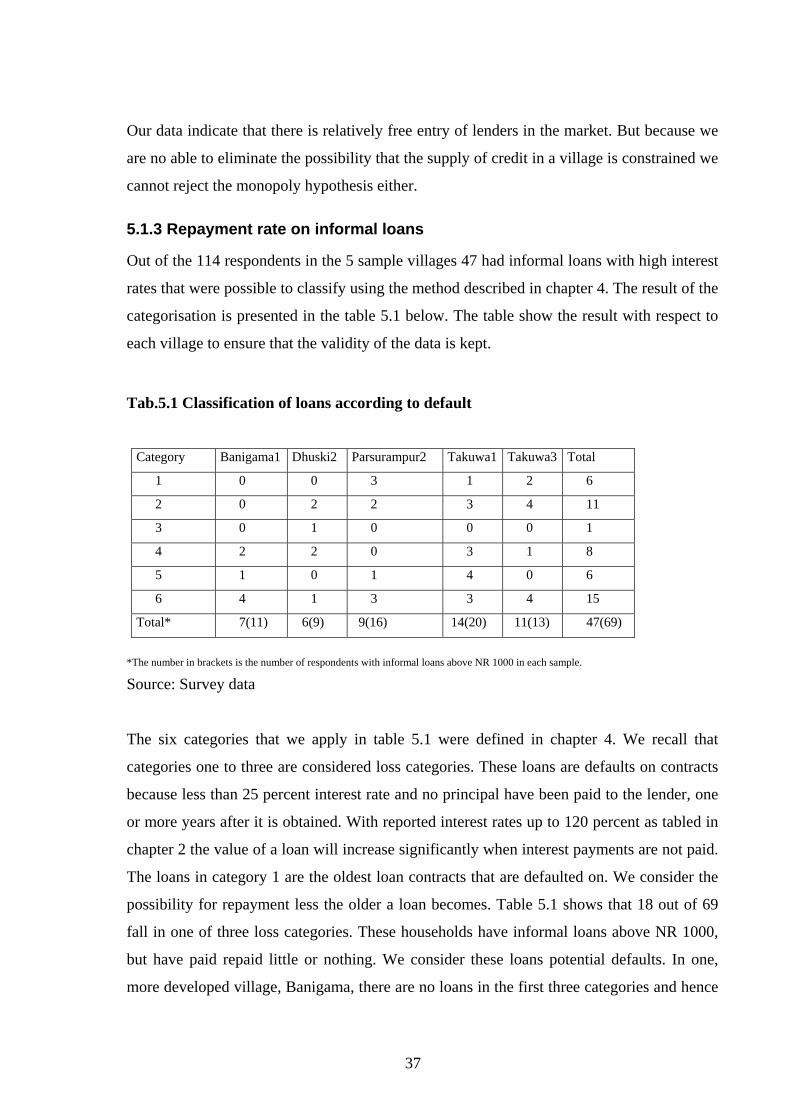
Our data indicate that there is relatively free entry of lenders in the market. But because we

are no able to eliminate the possibility that the supply of credit in a village is constrained we

cannot reject the monopoly hypothesis either.

5.1.3 Repayment rate on informal loans

Out of the 114 respondents in the 5 sample villages 47 had informal loans with high interest

rates that were possible to classify using the method described in chapter 4. The result of the

categorisation is presented in the table 5.1 below. The table show the result with respect to

each village to ensure that the validity of the data is kept.

Tab.5.1 Classification of loans according to default

Category Banigama1 Dhuski2 Parsurampur2 Takuwa1 Takuwa3 Total

1 0 0 3 1 2 6

2 0 2 2 3 4 11

3 0 1 0 0 0 1

4 2 2 0 3 1 8

5 1 0 1 4 0 6

6 4 1 3 3 4 15

Total* 7(11) 6(9) 9(16) 14(20) 11(13) 47(69)

*The number in brackets is the number of respondents with informal loans above NR 1000 in each sample.

Source: Survey data

The six categories that we apply in table 5.1 were defined in chapter 4. We recall that

categories one to three are considered loss categories. These loans are defaults on contracts

because less than 25 percent interest rate and no principal have been paid to the lender, one

or more years after it is obtained. With reported interest rates up to 120 percent as tabled in

chapter 2 the value of a loan will increase significantly when interest payments are not paid.

The loans in category 1 are the oldest loan contracts that are defaulted on. We consider the

possibility for repayment less the older a loan becomes. Table 5.1 shows that 18 out of 69

fall in one of three loss categories. These households have informal loans above NR 1000,

but have paid repaid little or nothing. We consider these loans potential defaults. In one,

more developed village, Banigama, there are no loans in the first three categories and hence

37

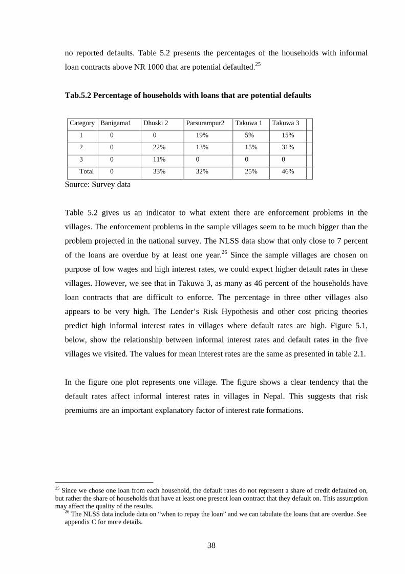
no reported defaults. Table 5.2 presents the percentages of the households with informal

loan contracts above NR 1000 that are potential defaulted.25

Tab.5.2 Percentage of households with loans that are potential defaults

Category Banigama1 Dhuski 2 Parsurampur2 Takuwa 1 Takuwa 3

1 0 0 19% 5% 15%

2 0 22% 13% 15% 31%

3 0 11% 0 0 0

Total 0 33% 32% 25% 46%

Source: Survey data

Table 5.2 gives us an indicator to what extent there are enforcement problems in the

villages. The enforcement problems in the sample villages seem to be much bigger than the

problem projected in the national survey. The NLSS data show that only close to 7 percent

of the loans are overdue by at least one year.26 Since the sample villages are chosen on

purpose of low wages and high interest rates, we could expect higher default rates in these

villages. However, we see that in Takuwa 3, as many as 46 percent of the households have

loan contracts that are difficult to enforce. The percentage in three other villages also

appears to be very high. The Lender’s Risk Hypothesis and other cost pricing theories

predict high informal interest rates in villages where default rates are high. Figure 5.1,

below, show the relationship between informal interest rates and default rates in the five

villages we visited. The values for mean interest rates are the same as presented in table 2.1.

In the figure one plot represents one village. The figure shows a clear tendency that the

default rates affect informal interest rates in villages in Nepal. This suggests that risk

premiums are an important explanatory factor of interest rate formations.

25 Since we chose one loan from each household, the default rates do not represent a share of credit defaulted on, but rather the share of households that have at least one present loan contract that they default on. This assumption may affect the quality of the results.

26 The NLSS data include data on “when to repay the loan” and we can tabulate the loans that are overdue. See appendix C for more details.

38

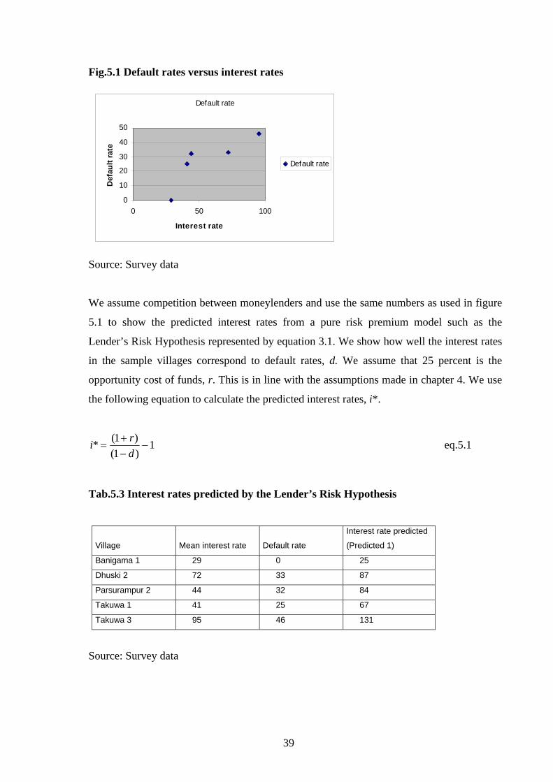
Fig.5.1 Default rates versus interest rates

Default rate

0

10

20

30

40

50

0 50 100

Interest rate

Def

ault

rate

Default rate

Source: Survey data

We assume competition between moneylenders and use the same numbers as used in figure

5.1 to show the predicted interest rates from a pure risk premium model such as the

Lender’s Risk Hypothesis represented by equation 3.1. We show how well the interest rates

in the sample villages correspond to default rates, d. We assume that 25 percent is the

opportunity cost of funds, r. This is in line with the assumptions made in chapter 4. We use

the following equation to calculate the predicted interest rates, i*.

1)1()1(* −

−+

=dri eq.5.1

Tab.5.3 Interest rates predicted by the Lender’s Risk Hypothesis

Village Mean interest rate Default rate

Interest rate predicted

(Predicted 1)

Banigama 1 29 0 25

Dhuski 2 72 33 87

Parsurampur 2 44 32 84

Takuwa 1 41 25 67

Takuwa 3 95 46 131

Source: Survey data

39

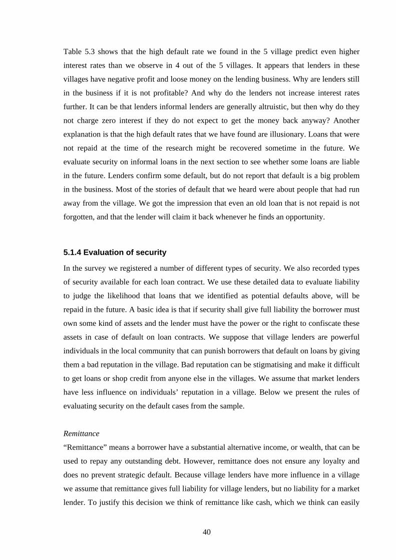
Table 5.3 shows that the high default rate we found in the 5 village predict even higher

interest rates than we observe in 4 out of the 5 villages. It appears that lenders in these

villages have negative profit and loose money on the lending business. Why are lenders still

in the business if it is not profitable? And why do the lenders not increase interest rates

further. It can be that lenders informal lenders are generally altruistic, but then why do they

not charge zero interest if they do not expect to get the money back anyway? Another

explanation is that the high default rates that we have found are illusionary. Loans that were

not repaid at the time of the research might be recovered sometime in the future. We

evaluate security on informal loans in the next section to see whether some loans are liable

in the future. Lenders confirm some default, but do not report that default is a big problem

in the business. Most of the stories of default that we heard were about people that had run

away from the village. We got the impression that even an old loan that is not repaid is not

forgotten, and that the lender will claim it back whenever he finds an opportunity.

5.1.4 Evaluation of security

In the survey we registered a number of different types of security. We also recorded types

of security available for each loan contract. We use these detailed data to evaluate liability

to judge the likelihood that loans that we identified as potential defaults above, will be

repaid in the future. A basic idea is that if security shall give full liability the borrower must

own some kind of assets and the lender must have the power or the right to confiscate these

assets in case of default on loan contracts. We suppose that village lenders are powerful

individuals in the local community that can punish borrowers that default on loans by giving

them a bad reputation in the village. Bad reputation can be stigmatising and make it difficult

to get loans or shop credit from anyone else in the villages. We assume that market lenders

have less influence on individuals’ reputation in a village. Below we present the rules of

evaluating security on the default cases from the sample.

Remittance

“Remittance” means a borrower have a substantial alternative income, or wealth, that can be

used to repay any outstanding debt. However, remittance does not ensure any loyalty and

does no prevent strategic default. Because village lenders have more influence in a village

we assume that remittance gives full liability for village lenders, but no liability for a market

lender. To justify this decision we think of remittance like cash, which we think can easily

40

be hidden from a market lender. Remittance in combination with a written contract gives

full liability for any lender.

Land and gold

The fact that borrowers possess land does not necessarily ensure that a lender can claim the

ownership of the land in case of default (Siamwalla et. al, 1993). We also gave examples of

some conditions under which collateral might fail to give any lender full liability in chapter

three. However, we met people in Nepal who had lost land to moneylenders, which indicate

that the threat of loosing land gives incentive to repay a loan whenever it is possible. The

borrowers are prepared to loose land if they fail to repay a loan. Possession of land or gold

therefore gives the lender full liability. In the data, only households with agricultural land in

addition to house land are registered with land. Gold deposits are easier to confiscate and is

more efficient as collateral. However, gold as security on informal loans is rare in Nepal.

Interlinkage

If the lender and the borrower have some other relationship prior to, or during the loan

period it is possible for the lender to get more accurate information about a borrower’s

credibility and such close relationships also improves the lenders possibility to enforce

repayment. Thus, these loans are relatively safe with respect to strategic defaults, but there

is no guarantee for the lender in case of involuntary default. Actually interlinkage loans are

more likely to be altruistic, compared to other loans, because the lender feels some

responsibility for his customers. A classical study of economic relations, within an Indian

caste system, confirms this and suggests that people might have incentives to help lower

caste members of the community to buy themselves a good fortune (S. Epstein, 1971).

Interlinkages probably also reduce the risk of lending because a lender is always able to

recover at least parts of a loan. Interlinkages give limited liability. Most “village-lender

loans” are expected to be interlinked.

Repeated credit relations

That a specific borrower has previously repaid a loan to the present lender tells us that the

borrower has a good credit history and has not used moral hazard in the past. Repeated loan

relations are a signal of honesty and low risk. Depending on the difficulties of building

creditability with a new lender, this prevents defaults. As long as the cost of repaying is less

than the cost of default, the borrower will have incentives to repay (Besley and Coate,

41

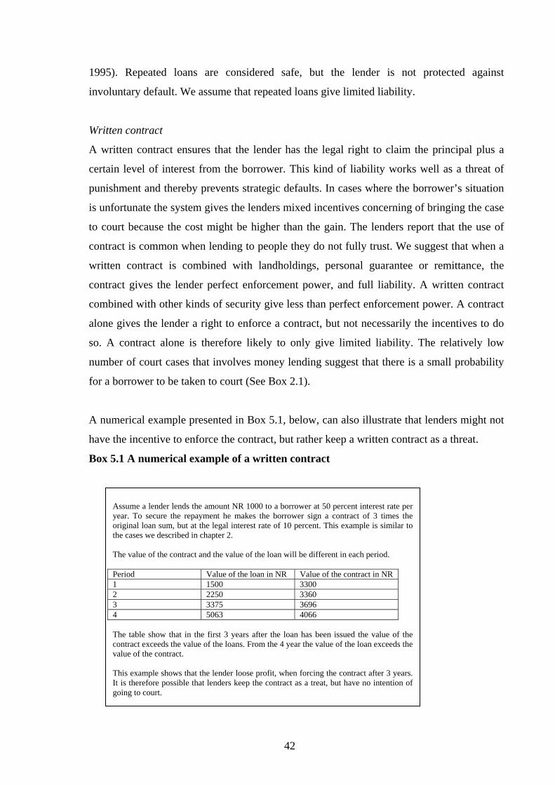
1995). Repeated loans are considered safe, but the lender is not protected against

involuntary default. We assume that repeated loans give limited liability.

Written contract

A written contract ensures that the lender has the legal right to claim the principal plus a

certain level of interest from the borrower. This kind of liability works well as a threat of

punishment and thereby prevents strategic defaults. In cases where the borrower’s situation

is unfortunate the system gives the lenders mixed incentives concerning of bringing the case

to court because the cost might be higher than the gain. The lenders report that the use of

contract is common when lending to people they do not fully trust. We suggest that when a

written contract is combined with landholdings, personal guarantee or remittance, the

contract gives the lender perfect enforcement power, and full liability. A written contract

combined with other kinds of security give less than perfect enforcement power. A contract

alone gives the lender a right to enforce a contract, but not necessarily the incentives to do

so. A contract alone is therefore likely to only give limited liability. The relatively low

number of court cases that involves money lending suggest that there is a small probability

for a borrower to be taken to court (See Box 2.1).

A numerical example presented in Box 5.1, below, can also illustrate that lenders might not

have the incentive to enforce the contract, but rather keep a written contract as a threat.

Box 5.1 A numerical example of a written contract

Assume a lender lends the amount NR 1000 to a borrower at 50 percent interest rate per year. To secure the repayment he makes the borrower sign a contract of 3 times the original loan sum, but at the legal interest rate of 10 percent. This example is similar to the cases we described in chapter 2. The value of the contract and the value of the loan will be different in each period. Period Value of the loan in NR Value of the contract in NR 1 1500 3300 2 2250 3360 3 3375 3696 4 5063 4066 The table show that in the first 3 years after the loan has been issued the value of the contract exceeds the value of the loans. From the 4 year the value of the loan exceeds the value of the contract. This example shows that the lender loose profit, when forcing the contract after 3 years. It is therefore possible that lenders keep the contract as a treat, but have no intention of going to court.

42

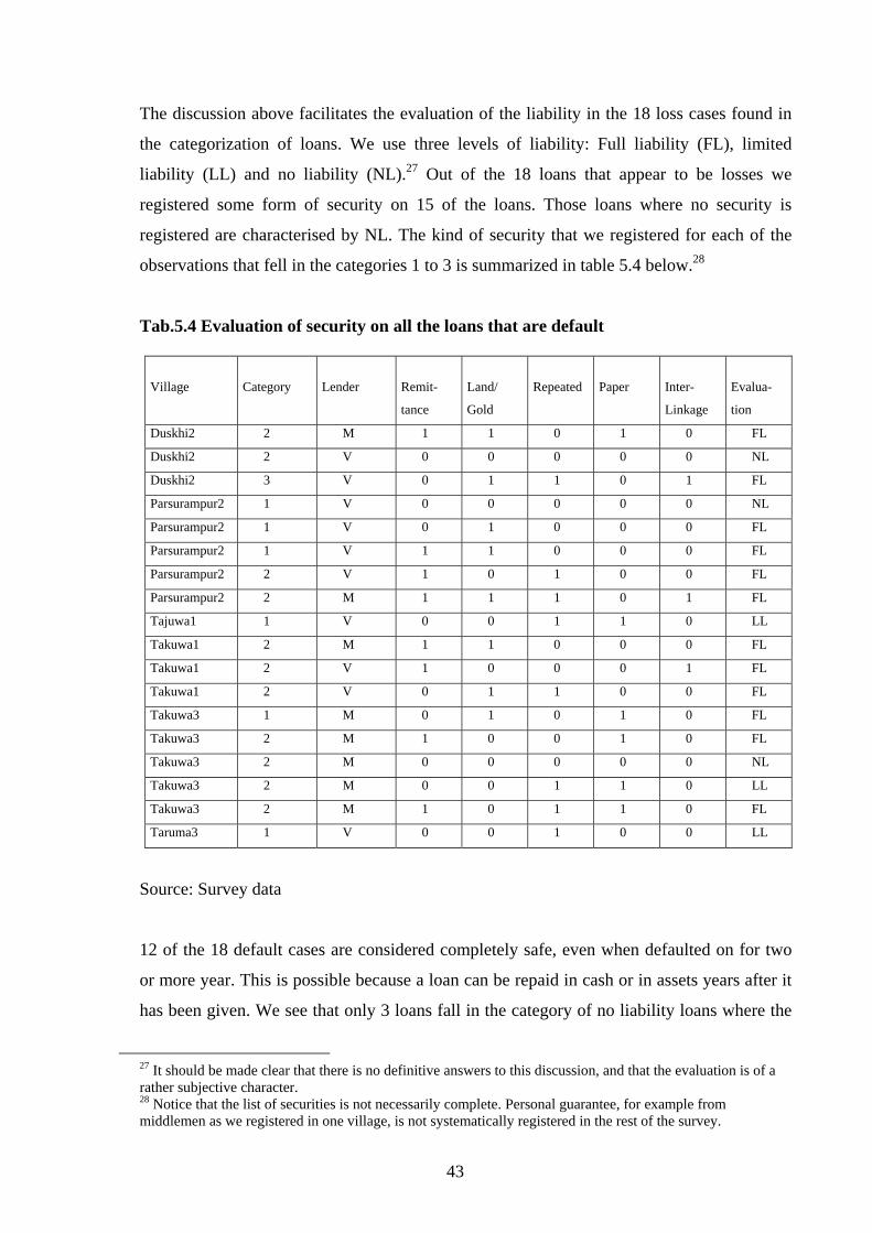
The discussion above facilitates the evaluation of the liability in the 18 loss cases found in

the categorization of loans. We use three levels of liability: Full liability (FL), limited

liability (LL) and no liability (NL).27 Out of the 18 loans that appear to be losses we

registered some form of security on 15 of the loans. Those loans where no security is

registered are characterised by NL. The kind of security that we registered for each of the

observations that fell in the categories 1 to 3 is summarized in table 5.4 below.28

Tab.5.4 Evaluation of security on all the loans that are default

Village

Category

Lender

Remit-

tance

Land/

Gold

Repeated

Paper

Inter-

Linkage

Evalua-

tion

Duskhi2 2 M 1 1 0 1 0 FL

Duskhi2 2 V 0 0 0 0 0 NL

Duskhi2 3 V 0 1 1 0 1 FL

Parsurampur2 1 V 0 0 0 0 0 NL

Parsurampur2 1 V 0 1 0 0 0 FL

Parsurampur2 1 V 1 1 0 0 0 FL

Parsurampur2 2 V 1 0 1 0 0 FL

Parsurampur2 2 M 1 1 1 0 1 FL

Tajuwa1 1 V 0 0 1 1 0 LL

Takuwa1 2 M 1 1 0 0 0 FL

Takuwa1 2 V 1 0 0 0 1 FL

Takuwa1 2 V 0 1 1 0 0 FL

Takuwa3 1 M 0 1 0 1 0 FL

Takuwa3 2 M 1 0 0 1 0 FL

Takuwa3 2 M 0 0 0 0 0 NL

Takuwa3 2 M 0 0 1 1 0 LL

Takuwa3 2 M 1 0 1 1 0 FL

Taruma3 1 V 0 0 1 0 0 LL

Source: Survey data

12 of the 18 default cases are considered completely safe, even when defaulted on for two

or more year. This is possible because a loan can be repaid in cash or in assets years after it

has been given. We see that only 3 loans fall in the category of no liability loans where the

27 It should be made clear that there is no definitive answers to this discussion, and that the evaluation is of a rather subjective character. 28 Notice that the list of securities is not necessarily complete. Personal guarantee, for example from middlemen as we registered in one village, is not systematically registered in the rest of the survey.

43

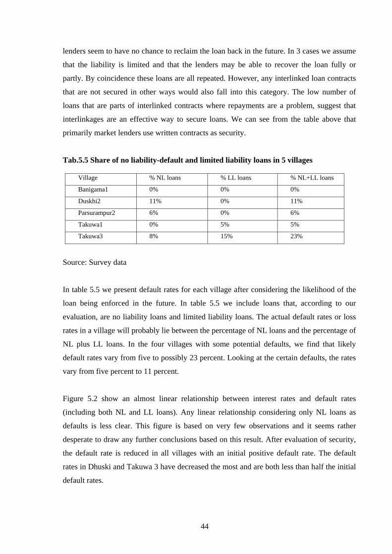
lenders seem to have no chance to reclaim the loan back in the future. In 3 cases we assume

that the liability is limited and that the lenders may be able to recover the loan fully or

partly. By coincidence these loans are all repeated. However, any interlinked loan contracts

that are not secured in other ways would also fall into this category. The low number of

loans that are parts of interlinked contracts where repayments are a problem, suggest that

interlinkages are an effective way to secure loans. We can see from the table above that

primarily market lenders use written contracts as security.

Tab.5.5 Share of no liability-default and limited liability loans in 5 villages

Village % NL loans % LL loans % NL+LL loans

Banigama1 0% 0% 0%

Duskhi2 11% 0% 11%

Parsurampur2 6% 0% 6%

Takuwa1 0% 5% 5%

Takuwa3 8% 15% 23%

Source: Survey data

In table 5.5 we present default rates for each village after considering the likelihood of the

loan being enforced in the future. In table 5.5 we include loans that, according to our

evaluation, are no liability loans and limited liability loans. The actual default rates or loss

rates in a village will probably lie between the percentage of NL loans and the percentage of

NL plus LL loans. In the four villages with some potential defaults, we find that likely

default rates vary from five to possibly 23 percent. Looking at the certain defaults, the rates

vary from five percent to 11 percent.

Figure 5.2 show an almost linear relationship between interest rates and default rates

(including both NL and LL loans). Any linear relationship considering only NL loans as

defaults is less clear. This figure is based on very few observations and it seems rather

desperate to draw any further conclusions based on this result. After evaluation of security,

the default rate is reduced in all villages with an initial positive default rate. The default

rates in Dhuski and Takuwa 3 have decreased the most and are both less than half the initial

default rates.

44

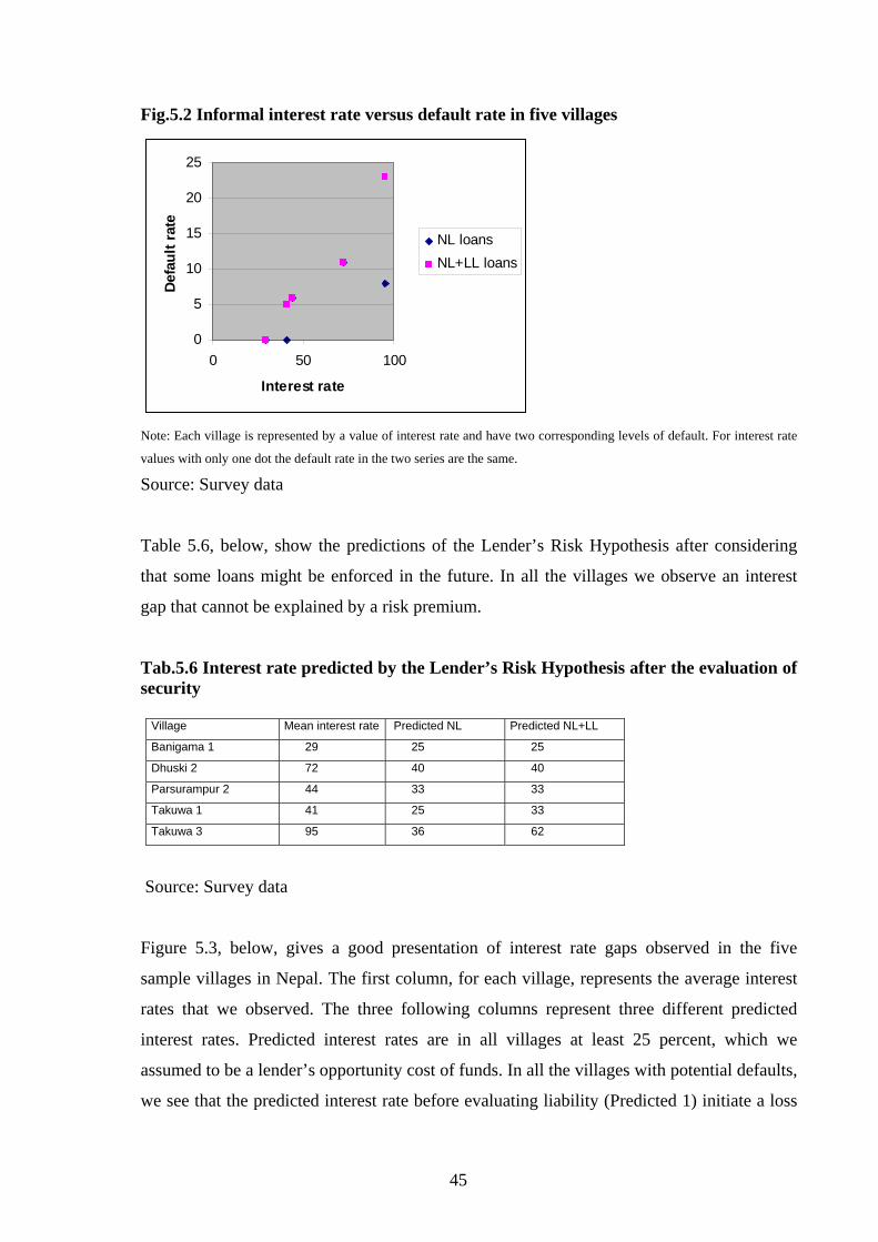
Fig.5.2 Informal interest rate versus default rate in five villages

0

5

10

15

20

25

0 50 100

Interest rate

Defa

ult r

ate

NL loansNL+LL loans

Note: Each village is represented by a value of interest rate and have two corresponding levels of default. For interest rate

values with only one dot the default rate in the two series are the same.

Source: Survey data

Table 5.6, below, show the predictions of the Lender’s Risk Hypothesis after considering

that some loans might be enforced in the future. In all the villages we observe an interest

gap that cannot be explained by a risk premium.

Tab.5.6 Interest rate predicted by the Lender’s Risk Hypothesis after the evaluation of security

Village Mean interest rate Predicted NL Predicted NL+LL

Banigama 1 29 25 25

Dhuski 2 72 40 40

Parsurampur 2 44 33 33

Takuwa 1 41 25 33

Takuwa 3 95 36 62

Source: Survey data

Figure 5.3, below, gives a good presentation of interest rate gaps observed in the five

sample villages in Nepal. The first column, for each village, represents the average interest

rates that we observed. The three following columns represent three different predicted

interest rates. Predicted interest rates are in all villages at least 25 percent, which we

assumed to be a lender’s opportunity cost of funds. In all the villages with potential defaults,

we see that the predicted interest rate before evaluating liability (Predicted 1) initiate a loss

45

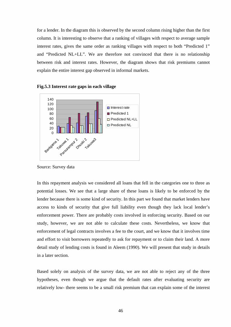
for a lender. In the diagram this is observed by the second column rising higher than the first

column. It is interesting to observe that a ranking of villages with respect to average sample

interest rates, gives the same order as ranking villages with respect to both “Predicted 1”

and “Predicted NL+LL”. We are therefore not convinced that there is no relationship

between risk and interest rates. However, the diagram shows that risk premiums cannot

explain the entire interest gap observed in informal markets.

Fig.5.3 Interest rate gaps in each village

020406080

100120140

Baniga

ma 1

Taku

wa 1

Parsura

mpur 2

Dhusk

i 2

Taku

wa3

Interest rate

Predicted 1

Predicted NL+LL

Predicted NL

Source: Survey data

In this repayment analysis we considered all loans that fell in the categories one to three as

potential losses. We see that a large share of these loans is likely to be enforced by the

lender because there is some kind of security. In this part we found that market lenders have

access to kinds of security that give full liability even though they lack local lender’s

enforcement power. There are probably costs involved in enforcing security. Based on our

study, however, we are not able to calculate these costs. Nevertheless, we know that

enforcement of legal contracts involves a fee to the court, and we know that it involves time

and effort to visit borrowers repeatedly to ask for repayment or to claim their land. A more

detail study of lending costs is found in Aleem (1990). We will present that study in details

in a later section.

Based solely on analysis of the survey data, we are not able to reject any of the three

hypotheses, even though we argue that the default rates after evaluating security are

relatively low- there seems to be a small risk premium that can explain some of the interest

46

rates. However, we look at conclusions made from other empirical studies to discriminate

between high searching costs and monopoly rent due to capacity constraints.

5.2 Relevant previous empirical studies

In a recent paper Hatlebakk (2000) is testing a model a cost-pricing monopolistic

competitive model with asymmetric information on the NLSS data set from Nepal.

Hatlebakk assumes that interest rate depends on risk related variables like caste, land value

and loan size and argues that the data show no significant effect of these variables on the

interest rate. Based on these conclusions he finds little support for the model and concludes

that the high interest rates in Nepal are not due to lending costs.

If lending costs determine the interest rate, we should be able to identify variables that

determine costs, and thus interest rates. The risk-premium hypothesis implies that interest

rates increase in the lender’s cost of default. The cost of default is in turn likely to be

smaller the higher is the borrowers’ wealth, as measured by land value. Similarly, the cost

of default is likely to increase in the loans size. On the other hand, the average screening

costs are likely to be smaller the larger the loan. The total effect might be a U-shaped

relation as modelled by Bell (1990). However, adjusting for indignity, we find no significant

effect of loan size on the equilibrium interest rates. Furthermore, we find no significant

effect of land value on the interest rates. 29

The conclusions above are based on assumptions made on how land value and loan size

affect risk. If there is no relationship between default and the risk related factors like land

and loan size, or land is not efficient to ensure full liability Hatlebakk’s study could possibly

overlooks a risk premium in the market. Our data confirms a low risk premium, but our

survey data shows a strong tendency toward higher interest rates in villages with relatively

higher rates defaults. Our result shows that there are potentially high costs in chasing

delinquent loans and enforcing security. This is not captured in Hatlebakk’s testing.

In the same paper Hatlebakk is also testing a model of a collusive oligopoly with full

information on the NLSS data from Nepal. This model gives predictions about how interest

rates are set in different segments of a village. We already introduced this theory briefly in

29 “Will more credit increase the interest rates in rural Nepal?” M. Hatlebakk (2000), pp.19

47

chapter 3. The model used in Hatlebakk (2000) predicts that interest rates in villages with

low lending capacities are determined by the borrowers’ demand for credit in the village.

This implies that in villages with low lending capacity the interest rates will be high. This

result is only valid if default rates are low and costs related to defaults are low. Again, our

village sample confirms low default rates, but not necessary low costs due to reduction of

risk. For villages with higher lending capacities, the model predicts that high interest rates

may be a certain interval of lending capacities where high interest rates are a result of

collusive monopoly pricing. In both cases the lenders might earn profit. For villages without

lending constraints, the market will be competitive with zero profit. Based on the test of this

model against data from Nepal, Hatlebakk is not able to identify a capacity-interval that

shows a significantly increasing price function. He is thus not able to distinguish between a

competitive and a collusive price setting in villages with higher lending capacity. However,

because he finds limited support in the first test of a cost pricing model of informal interest

rates formation, he concludes that his study give more support to the model of capacity

constrained lending with possible collusive pricing of interest rates. An important

contribution of this paper is to determine the lending capacities for villages in Nepal. He

uses land value above a certain critical value as an indicator of individual lending capacities.

The study concludes that most villages are capacity constrained. According to this result we

should expect that most of the high interest/low caste villages we chose to have in our

sample are capacity constrained. We mentioned in the analysis that in Takuwa 3 there was

few local lenders. In this particular village we observed the highest average interest rate. In

all the villages we observed both local and external lenders. This implies that credit is

constrained within a village, since borrowers always look for local sources of credit before

they turned to market lenders. In another village, Banigama, which is more developed than

the other villages we have in the sample, we observed lower interest rates. This village is

most likely not capacity constrained and as the model used by Hatlebakk predicts, the

interest rates in this village may reflect full competition.

Hatlebakk’s study is interesting because it shows that actual interest rates in capacity

constrained villages need not systematically correspond to the predicted interest based on

default and lending costs, but rather depends on the supply of credit. Variations in interest

rates between villages in our sample can therefore be explained by differences in supply of

credit.

48

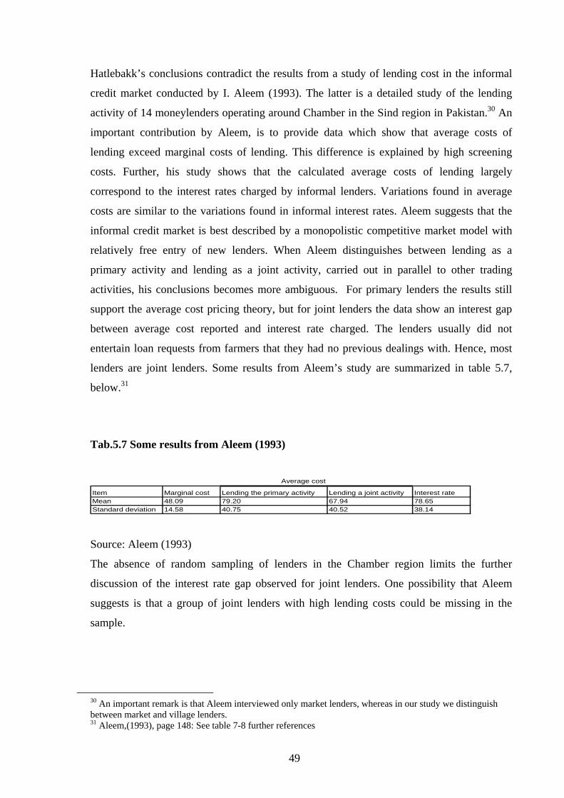
Hatlebakk’s conclusions contradict the results from a study of lending cost in the informal

credit market conducted by I. Aleem (1993). The latter is a detailed study of the lending

activity of 14 moneylenders operating around Chamber in the Sind region in Pakistan.30 An

important contribution by Aleem, is to provide data which show that average costs of

lending exceed marginal costs of lending. This difference is explained by high screening

costs. Further, his study shows that the calculated average costs of lending largely

correspond to the interest rates charged by informal lenders. Variations found in average

costs are similar to the variations found in informal interest rates. Aleem suggests that the

informal credit market is best described by a monopolistic competitive market model with

relatively free entry of new lenders. When Aleem distinguishes between lending as a

primary activity and lending as a joint activity, carried out in parallel to other trading

activities, his conclusions becomes more ambiguous. For primary lenders the results still

support the average cost pricing theory, but for joint lenders the data show an interest gap

between average cost reported and interest rate charged. The lenders usually did not

entertain loan requests from farmers that they had no previous dealings with. Hence, most

lenders are joint lenders. Some results from Aleem’s study are summarized in table 5.7,

below.31

Tab.5.7 Some results from Aleem (1993)

Average cost

Item Marginal cost Lending the primary activity Lending a joint activity Interest rateMean 48.09 79.20 67.94 78.65Standard deviation 14.58 40.75 40.52 38.14

Source: Aleem (1993)

The absence of random sampling of lenders in the Chamber region limits the further

discussion of the interest rate gap observed for joint lenders. One possibility that Aleem

suggests is that a group of joint lenders with high lending costs could be missing in the

sample.

30 An important remark is that Aleem interviewed only market lenders, whereas in our study we distinguish between market and village lenders. 31 Aleem,(1993), page 148: See table 7-8 further references

49

The average costs include estimates of the screening activity, opportunity cost of funding,

value of time spent chasing delinquent loans and so on. The estimation includes a valuation

of the lender’s time. This is a complicated issue, because if lending is a joint activity, it is

difficult for the lender to report the amount of time spent on which business if the

businesses are interlinked. Crucial to the result is also the assumption that the opportunity

cost of funds equals the marginal cost of funds, on average 23 percent for the 14 lenders,

rather than the prevailing bank rate of 10 percent. In our data analysis we assumed that the

opportunity cost of funds equals 25 percent, which is higher than the bank rate at 18 percent

for loans in the ADB bank at the time of research. Without these assumptions the interest

rate gaps observed in both studies would be larger.

Aleem’s study also describes a typical screening and monitoring process in details. He finds

that lenders must invest a substantial amount of time, resources and efforts in evaluating a

borrower’s credibility. Lenders typically issue small test loans to first-time borrowers.

Aleem concludes that the screening process is costly for these market lenders and that these

costs reflect the interest rates that these lenders charge on informal loans. However, we have

no data to conduct similar calculations.

A main task in this data analysis has been to determine the default rate on informal loans in

Nepal. Aleem also investigate the repayment of informal loans as a part of his study of

lending costs in Pakistan. The average default rate for the 14 lenders is 2.7 percent. New

lenders face a higher rate of default than more well-established lenders in the survey. Aleem

concludes that default and interest lost due to delinquent loans only count for a relatively

small part of the total interest charges. The default rate on small “test loans”, offered in the

screening period, is higher. This results in a high rejection rate on new loan applicants. Test

loans are used by most of the lenders to lower the risk of bad debt.32 Moneylenders report a

higher share of delinquency. All 14 reported a problem of late repayment. On average 15

percent of the loans were likely to be delayed. The lenders face a higher risk of default on

these loans, and there are interest loss and costs of chasing overdue loans. 5 out of 14

lenders say they do not charge extra interest for late repayment. The rest only accept such

losses under specific circumstances.33 Very few loans were secured with collateral, but 78

percent of the customers were repeated costumers.

32 Aleem gives a longer intuitive explanation to how test loans lower risk. See page 145, Aleem (1993) 33 See Table 7-3, Aleem (1993) for details.

50

Our study shows little evidence of expensive screening, but we find that there are large

enforcement problems. Aleem found that the costs related to enforcement problems could

only count for a small share of the interest rates. We are not able to calculate these costs

based on out data. However, if this result from Aleem applies to Nepal it implies that

lending costs in Nepal are relatively lower than those observed in Pakistan due to low

screening costs.

Few studies we know about have been made on repayment. Raj (1979) published a paper

where he is reflecting on the applicability of Keynesian economic theory on the agrarian

economies in developing countries. One topic that he discusses is default and mark up on

informal loans. Raj argues different perspectives and explanations of high interest rates. In

his paper he discusses the data from an “All Indian Rural Credit survey”. In this survey two-

thirds of the moneylenders say that they consider less than 10 percent of the loans as

doubtful. Raj concludes that the Lender’s Risk Hypothesis based on U Tun Wai (1957)

cannot alone explain the high interest rates charged on informal loans.34 This conclusion is

similar to our conclusion based on our observations on default. Raj suggests we look in the

direction of credit rationing to explain high informal interest rates. We described briefly a

theory of credit rationing in the theoretical approach. In theory, interest rates can reflect

both costs and monopoly rent when there is credit rationing. This gives some similar

implications as the capacity constrained model- that we do not necessary observe any

systematic relationship between predicted interest rates based on default and the observed

interest rates.

5.3 Preliminary conclusions

Based solely on our experience from Nepal we are no able to reject any of the three

hypotheses about interest rate formation. We summarize outcomes of the analysis below.

An estimate of potential risk represented by default rates before evaluating the liability of

any loans, show that there are large enforcement problems in four out of five villages in our

sample. We find that the predicted interest rate based on the potential risk projected

negative profit in four villages. This implied that these initial default rates were illusionary.

34 Conversely, Raj says nothing about the default rate that the rest, 1/3, of the lenders report.

51

After considering the liability of each loss contract we found significantly lower default

rates, but we still observe a tendency of higher interest rates in villages with relatively high

default rates. However, in line with Raj we conclude that the interest rate gaps that we

observe between informal and formal interest rates in Nepal cannot alone be explained by

risk premiums.

Another observation that was emphasized during the analysis was that we observed no

significant difference between the interest rates charged by village lenders and market

lenders in four out of five villages. We argued that this can indicate both competition and

price collusion.

We observe a dual informal credit market where both village and external market lenders

provide credit in each village. Market lenders seem to be a part of a “semiformal” credit

market, where written contracts ensure legal enforcement. That market lenders have access

to kinds of security that ensure full liability make them able to compete with local lenders at

village level. We found in line with Aleem that there is relatively free entry into the market.

This implies that there is some competition in the market.

Aleem finds that screening costs are high, but our experience is that even less informed

market lenders are able to overcome the screening problem without large investments

because they also have access to efficient ways to secure loans. However, our data indicated

that there are large enforcement problems and possibly costs due to chasing overdue loans

for both types of lenders. This implied that we cannot reject the possibility of high

transaction costs due to expensive searching activities.

The relatively free entry for new lenders and the high enforcement costs gave strong

indicators of a monopolistic competitive modelling of the informal credit market. However,

a previous study of the informal credit market in Nepal concludes that high interest rates in

Nepal do not reflect high lending costs (Hatlebakk, 2000). This conclusion relies on several

assumptions about risk. We argued in the analysis that the study possibly overlooks any

risk premiums and enforcement costs.

In the same study Hatlebakk (2000) shows that rural villages in Nepal are capacity

constrained. In these villages the informal interest rates do not have to reflect cost of lending

52

and default. Interest rates can rather be determined by the demand for credit in these villages

and lenders can earn positive profit and monopoly rent. We suggest that in villages with

relatively high risk of default there can be credit constrains because lenders lack incentives

to compete and hence ration credit. Credit rationing models originally explain interest rates

below equilibrium level, but in a competitive aspect the model can also explain high interest

rates. In villages that are more developed the risk of default seems to be lower. In these

villages there are no credit constraints and the informal credit market is likely to be

competitive.

53

6. Conclusions The data survey show that the average annual interest rates on informal loans vary from 29

percent to 95 percent. At the time of the research the Agricultural Development Bank

providing loans in the same area charged an interest rate of 18 percent per year. The

observed interest rate gaps between formal and informal interest rates are confirmed by data

from a national household survey from 1996.

In theory there exist competing perspectives of the informal credit market. Based on a

selection of theoretical contributions we conclude that high informal interest rates are either

due to high costs or monopoly rent. We distinguish three elements that affect the level of

interest rates that we observe in the informal market. These are the basis for the three

hypotheses about interest rate formation: The risk premium hypothesis, the searching cost

hypotheses and the monopoly rent hypothesis.

An empirical evaluation of the hypotheses finds that based solely on the data survey from

Nepal we are not able to reject any of the three possible explanations of high interest rates.

We identify positive, but low default rates in four of the five sample villages. This implies

that the risk premiums charged on informal loans are low. The high potential default rates

indicate that informal lending is risky, and we suggest that there are high enforcement costs

either due to chasing delinquent loans or due to cost of enforcing security. A main task in

this part of the analysis was to present rules for evaluating liability on overdue loans.

Further, we learned from the experience of Nepal that screening costs are generally low. For

village lenders adverse selection and moral hazard are largely overcome by personal

relationships and interlinked contracts. For market lenders these problems are solved by

access to security that gives full liability.

We conclude that the informal credit market in Nepal is best described by a monopolistic

competitive model with free entry where interest rates reflect transaction costs, mainly due

to risk premiums and enforcement costs. However, we argue that there can be credit

rationing in villages with relatively high risk of default. Based on the data survey we are not

able to discuss this further.

54

References Aleem. I. (1993). Imperfect Information, Screening, and the Cost of informal Lending: A Study of a Rural Credit Market in Pakistan, in Hoff and Stiglitz (1993). The economics of rural organization; theory, practice, and policy, Oxford University Press, Oxford, pp. 131-154

Bardhan, P. and Udry, C. (1999). Development microeconomics, Oxford University Press, Oxford, chapter 7

Basu, K. (1994). Agrarian Questions. Oxford University Press, Oxford, pp. 1-17 Basu, K. (1997). Analytical Development Economics. The Less Developed Economy Revisited. MIT Press, pp. 267-316 Basu, K., Bell, C. and Bose, P. (1999). Interlinkage, Limited Liability, and Strategic Interaction, Policy Research working Paper 2134, World Bank, June 1999. Bell, C. (1990). Interaction between Institutional and Informal Credit Agencies in Rural India. The World Economic Review, 4 3 (1990), pp. 297-327 Besley, T. and Coate, S. (1995). Group Lending, Repayment Incentives and social Collateral. Journal of Development Economics 46, pp. 1-18. Central Bureau of Statistics (2002). Statistical Pocket Book Nepal 2002, CBS, Thapathali, Kathmandu, Nepal Coate, S. (1993). Reciprocity without commitment. Characteristics and performance of informal insurance arrangements. Journal of Development Economics, Vol. 40, Issue 1, pp. 1-24 Epstein, S (1971) Economic Development and social Change in South India, in Dalton, G. (1971) edited. Economic Development and social Change, The Natural history Press, New York, pp. 460-491 Hatlebakk, M. (2000). Will More Credit Increase Interest Rates in Rural Nepal?, in Essays on Poverty in Informal Rural Markets. University of Bergen, pp.1-62 Hoff, K. and Stiglitz, J.E. (1997). Moneylenders and bankers: price-increasing subsidies in a monopolistically competitive market. Journal of Development Economics, 55 (1998), pp. 485-518. Hoff, K. and Stiglitz, J.E. (1993). The economics of rural organization; theory, practice, and policy, Oxford University Press, Oxford http://hdr.undp.org/reports/global/2003/ Human Development Report (2004), 2005-02-24

55

Lewis-Beck, Bryman and Liao, editors (2004). The SAGE Encyclopaedia of Social Science Research Methods, SAGE Publications, Inc. Page: 957(3) Raj, K.N. (1979). Keynesian Economics and Agrarian Economics, in Rao and Joshi (1979). Reflections on Economic Development and social Change. Allied Publishers Private Limited, India, pp. 100-130 Ray, D. (1998). Development economics, Princton University Press, page 529-589 Siamvalla et. Al. (1993). The Thai Rural Credit System and Elements of a Theory: Public Subsidies, Private Information, and Segmented Markets, in Hoff and Stiglitz (1993). The economics of rural organization; theory, practice, and policy, Oxford University Press, Oxford, page 154-185 Stiglitz, J.E. and Weiss, A. (1981). Credit rationing in markets with imperfect information. The American Economic Review 71 3 (1981), pp. 393–409. (Tun Wai, U. (1958). Interest rates outside organised money markets of underdeveloped countries. I.M.F Staff papers 6.) Varian, H. R. (1999). Intermediate Microeconomics. A Modern Approach. USA www.worldbank.org/lsms/country/nepal/nep96docs/htmlNepal Living Standard survey (1996), 2005-02-24 Yadav et al. (1992). S. Yadav, K. Otsuka and C.C. David , Segmentation in rural financial markets: the case of Nepal. World Development 20 3 (1992), pp. 423–436.

56

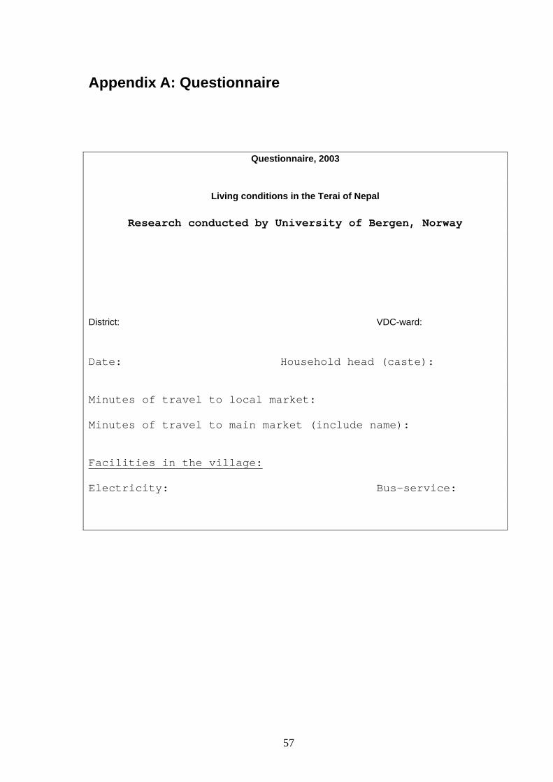
Appendix A: Questionnaire

Questionnaire, 2003

Living conditions in the Terai of Nepal

Research conducted by University of Bergen, Norway

District: VDC-ward: Date: Household head (caste): Minutes of travel to local market: Minutes of travel to main market (include name): Facilities in the village: Electricity: Bus-service:

57

1

58

2

59

3

60

4

61

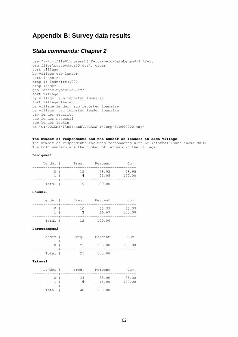
Appendix B: Survey data results

Stata commands: Chapter 2 use "\\\cmifile01\norunnh$\Feltarbeid\Databehandlin\felt org.filer\syrveydata03.dta", clear sort village by village tab lender sort loansize drop if loansize<1000 drop lender gen lender=typeofle=="m" sort village by village: sum reported loansize sort village lender by village lender: sum reported loansize by village: reg reported lender loansize tab lender security tab lender nosecuri tab lender lackin do "C:\DOCUME~1\norunnh\LOCALS~1\Temp\STD000000.tmp" The number of respondents and the number of lenders in each village The number of respondents includes respondents with no informal loans above NR1000. The bold numbers are the number of lenders in the village. Banigama1 Lender | Freq. Percent Cum. ------------+----------------------------------- 0 | 15 78.95 78.95 1 | 4 21.05 100.00 ------------+----------------------------------- Total | 19 100.00 Dhuski2 Lender | Freq. Percent Cum. ------------+----------------------------------- 0 | 10 83.33 83.33 1 | 2 16.67 100.00 ------------+----------------------------------- Total | 12 100.00 Parsurampur2 Lender | Freq. Percent Cum. ------------+----------------------------------- 0 | 23 100.00 100.00 ------------+----------------------------------- Total | 23 100.00 Takuwa1 Lender | Freq. Percent Cum. ------------+----------------------------------- 0 | 34 85.00 85.00 1 | 6 15.00 100.00 ------------+----------------------------------- Total | 40 100.00

62

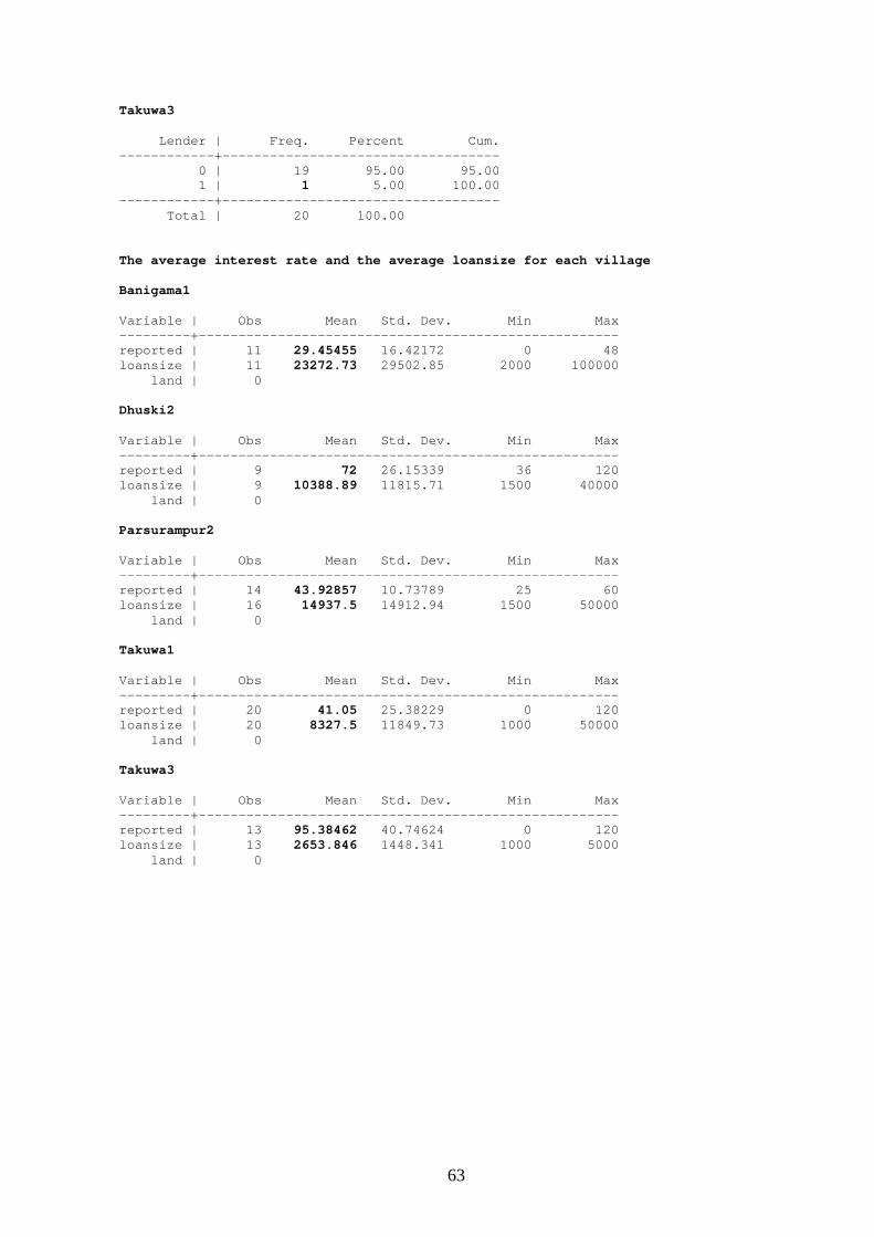
Takuwa3 Lender | Freq. Percent Cum. ------------+----------------------------------- 0 | 19 95.00 95.00 1 | 1 5.00 100.00 ------------+----------------------------------- Total | 20 100.00 The average interest rate and the average loansize for each village Banigama1 Variable | Obs Mean Std. Dev. Min Max ---------+----------------------------------------------------- reported | 11 29.45455 16.42172 0 48 loansize | 11 23272.73 29502.85 2000 100000 land | 0 Dhuski2 Variable | Obs Mean Std. Dev. Min Max ---------+----------------------------------------------------- reported | 9 72 26.15339 36 120 loansize | 9 10388.89 11815.71 1500 40000 land | 0 Parsurampur2 Variable | Obs Mean Std. Dev. Min Max ---------+----------------------------------------------------- reported | 14 43.92857 10.73789 25 60 loansize | 16 14937.5 14912.94 1500 50000 land | 0 Takuwa1 Variable | Obs Mean Std. Dev. Min Max ---------+----------------------------------------------------- reported | 20 41.05 25.38229 0 120 loansize | 20 8327.5 11849.73 1000 50000 land | 0 Takuwa3 Variable | Obs Mean Std. Dev. Min Max ---------+----------------------------------------------------- reported | 13 95.38462 40.74624 0 120 loansize | 13 2653.846 1448.341 1000 5000 land | 0

63

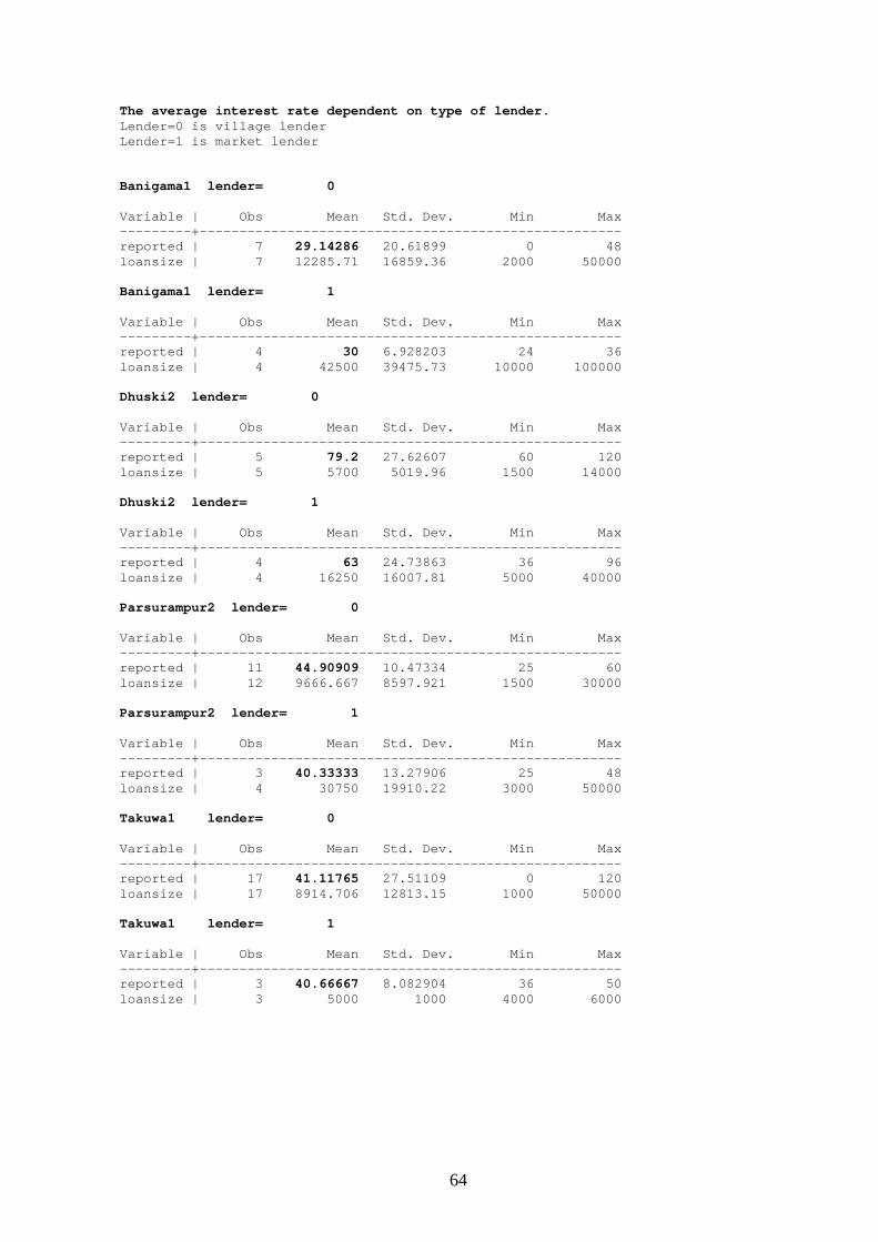
The average interest rate dependent on type of lender. Lender=0 is village lender Lender=1 is market lender Banigama1 lender= 0 Variable | Obs Mean Std. Dev. Min Max ---------+----------------------------------------------------- reported | 7 29.14286 20.61899 0 48 loansize | 7 12285.71 16859.36 2000 50000 Banigama1 lender= 1 Variable | Obs Mean Std. Dev. Min Max ---------+----------------------------------------------------- reported | 4 30 6.928203 24 36 loansize | 4 42500 39475.73 10000 100000 Dhuski2 lender= 0 Variable | Obs Mean Std. Dev. Min Max ---------+----------------------------------------------------- reported | 5 79.2 27.62607 60 120 loansize | 5 5700 5019.96 1500 14000 Dhuski2 lender= 1 Variable | Obs Mean Std. Dev. Min Max ---------+----------------------------------------------------- reported | 4 63 24.73863 36 96 loansize | 4 16250 16007.81 5000 40000 Parsurampur2 lender= 0 Variable | Obs Mean Std. Dev. Min Max ---------+----------------------------------------------------- reported | 11 44.90909 10.47334 25 60 loansize | 12 9666.667 8597.921 1500 30000 Parsurampur2 lender= 1 Variable | Obs Mean Std. Dev. Min Max ---------+----------------------------------------------------- reported | 3 40.33333 13.27906 25 48 loansize | 4 30750 19910.22 3000 50000 Takuwa1 lender= 0 Variable | Obs Mean Std. Dev. Min Max ---------+----------------------------------------------------- reported | 17 41.11765 27.51109 0 120 loansize | 17 8914.706 12813.15 1000 50000 Takuwa1 lender= 1 Variable | Obs Mean Std. Dev. Min Max ---------+----------------------------------------------------- reported | 3 40.66667 8.082904 36 50 loansize | 3 5000 1000 4000 6000

64

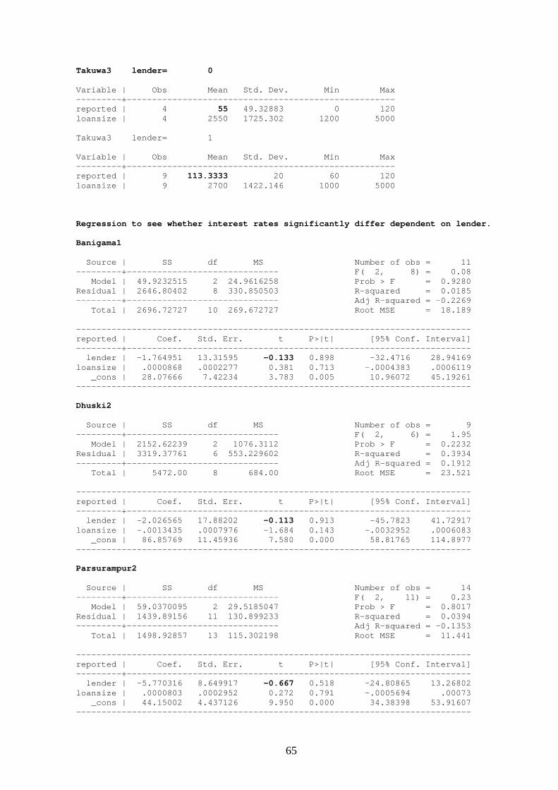
Takuwa3 lender= 0 Variable | Obs Mean Std. Dev. Min Max ---------+----------------------------------------------------- reported | 4 55 49.32883 0 120 loansize | 4 2550 1725.302 1200 5000 Takuwa3 lender= 1 Variable | Obs Mean Std. Dev. Min Max ---------+----------------------------------------------------- reported | 9 113.3333 20 60 120 loansize | 9 2700 1422.146 1000 5000 Regression to see whether interest rates significantly differ dependent on lender. Banigama1 Source | SS df MS Number of obs = 11 ---------+------------------------------ F( 2, 8) = 0.08 Model | 49.9232515 2 24.9616258 Prob > F = 0.9280 Residual | 2646.80402 8 330.850503 R-squared = 0.0185 ---------+------------------------------ Adj R-squared = -0.2269 Total | 2696.72727 10 269.672727 Root MSE = 18.189 ------------------------------------------------------------------------------ reported | Coef. Std. Err. t P>|t| [95% Conf. Interval] ---------+-------------------------------------------------------------------- lender | -1.764951 13.31595 -0.133 0.898 -32.4716 28.94169 loansize | .0000868 .0002277 0.381 0.713 -.0004383 .0006119 _cons | 28.07666 7.42234 3.783 0.005 10.96072 45.19261 ------------------------------------------------------------------------------ Dhuski2 Source | SS df MS Number of obs = 9 ---------+------------------------------ F( 2, 6) = 1.95 Model | 2152.62239 2 1076.3112 Prob > F = 0.2232 Residual | 3319.37761 6 553.229602 R-squared = 0.3934 ---------+------------------------------ Adj R-squared = 0.1912 Total | 5472.00 8 684.00 Root MSE = 23.521 ------------------------------------------------------------------------------ reported | Coef. Std. Err. t P>|t| [95% Conf. Interval] ---------+-------------------------------------------------------------------- lender | -2.026565 17.88202 -0.113 0.913 -45.7823 41.72917 loansize | -.0013435 .0007976 -1.684 0.143 -.0032952 .0006083 _cons | 86.85769 11.45936 7.580 0.000 58.81765 114.8977 ------------------------------------------------------------------------------ Parsurampur2 Source | SS df MS Number of obs = 14 ---------+------------------------------ F( 2, 11) = 0.23 Model | 59.0370095 2 29.5185047 Prob > F = 0.8017 Residual | 1439.89156 11 130.899233 R-squared = 0.0394 ---------+------------------------------ Adj R-squared = -0.1353 Total | 1498.92857 13 115.302198 Root MSE = 11.441 ------------------------------------------------------------------------------ reported | Coef. Std. Err. t P>|t| [95% Conf. Interval] ---------+-------------------------------------------------------------------- lender | -5.770316 8.649917 -0.667 0.518 -24.80865 13.26802 loansize | .0000803 .0002952 0.272 0.791 -.0005694 .00073 _cons | 44.15002 4.437126 9.950 0.000 34.38398 53.91607 ------------------------------------------------------------------------------

65

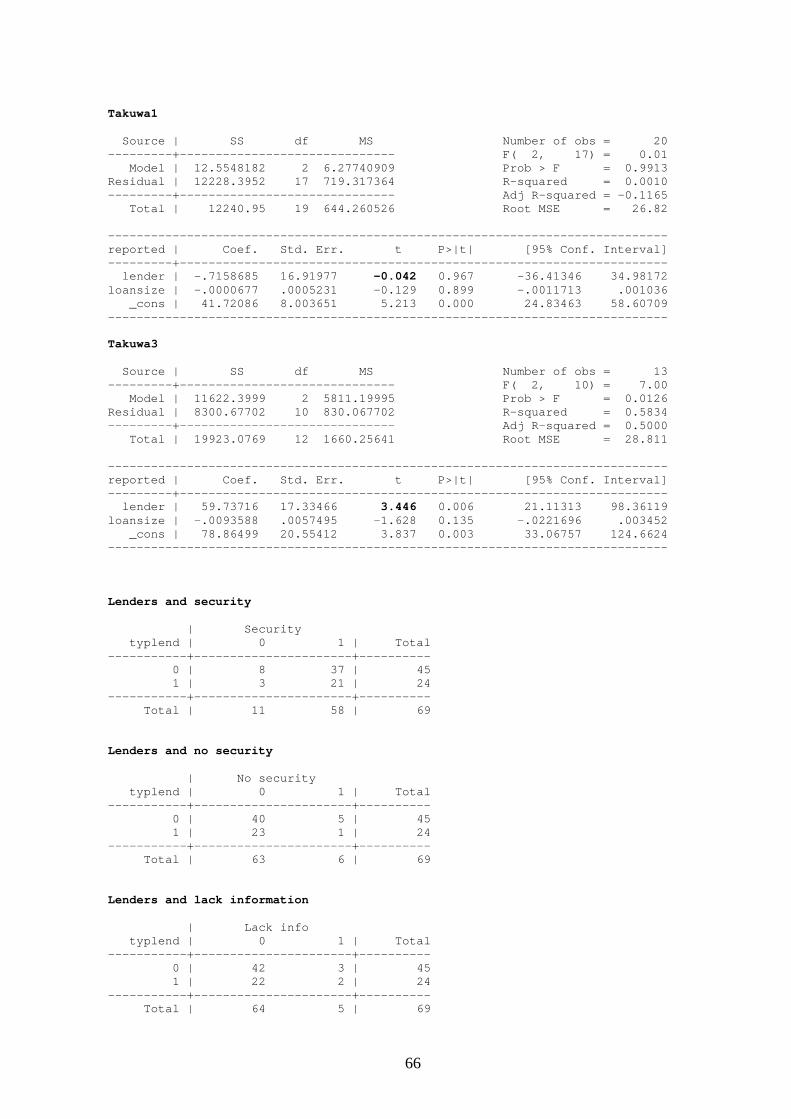
Takuwa1 Source | SS df MS Number of obs = 20 ---------+------------------------------ F( 2, 17) = 0.01 Model | 12.5548182 2 6.27740909 Prob > F = 0.9913 Residual | 12228.3952 17 719.317364 R-squared = 0.0010 ---------+------------------------------ Adj R-squared = -0.1165 Total | 12240.95 19 644.260526 Root MSE = 26.82 ------------------------------------------------------------------------------ reported | Coef. Std. Err. t P>|t| [95% Conf. Interval] ---------+-------------------------------------------------------------------- lender | -.7158685 16.91977 -0.042 0.967 -36.41346 34.98172 loansize | -.0000677 .0005231 -0.129 0.899 -.0011713 .001036 _cons | 41.72086 8.003651 5.213 0.000 24.83463 58.60709 ------------------------------------------------------------------------------ Takuwa3 Source | SS df MS Number of obs = 13 ---------+------------------------------ F( 2, 10) = 7.00 Model | 11622.3999 2 5811.19995 Prob > F = 0.0126 Residual | 8300.67702 10 830.067702 R-squared = 0.5834 ---------+------------------------------ Adj R-squared = 0.5000 Total | 19923.0769 12 1660.25641 Root MSE = 28.811 ------------------------------------------------------------------------------ reported | Coef. Std. Err. t P>|t| [95% Conf. Interval] ---------+-------------------------------------------------------------------- lender | 59.73716 17.33466 3.446 0.006 21.11313 98.36119 loansize | -.0093588 .0057495 -1.628 0.135 -.0221696 .003452 _cons | 78.86499 20.55412 3.837 0.003 33.06757 124.6624 ------------------------------------------------------------------------------ Lenders and security | Security typlend | 0 1 | Total -----------+----------------------+---------- 0 | 8 37 | 45 1 | 3 21 | 24 -----------+----------------------+---------- Total | 11 58 | 69 Lenders and no security | No security typlend | 0 1 | Total -----------+----------------------+---------- 0 | 40 5 | 45 1 | 23 1 | 24 -----------+----------------------+---------- Total | 63 6 | 69 Lenders and lack information | Lack info typlend | 0 1 | Total -----------+----------------------+---------- 0 | 42 3 | 45 1 | 22 2 | 24 -----------+----------------------+---------- Total | 64 5 | 69

66

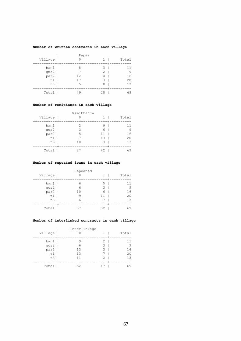
Number of written contracts in each village | Paper Village | 0 1 | Total -----------+----------------------+---------- ban1 | 8 3 | 11 gus2 | 7 2 | 9 par2 | 12 4 | 16 t1 | 17 3 | 20 t3 | 5 8 | 13 -----------+----------------------+---------- Total | 49 20 | 69 Number of remittance in each village | Remittance Village | 0 1 | Total -----------+----------------------+---------- ban1 | 2 9 | 11 gus2 | 3 6 | 9 par2 | 5 11 | 16 t1 | 7 13 | 20 t3 | 10 3 | 13 -----------+----------------------+---------- Total | 27 42 | 69 Number of repeated loans in each village | Repeated Village | 0 1 | Total -----------+----------------------+---------- ban1 | 6 5 | 11 gus2 | 6 3 | 9 par2 | 10 6 | 16 t1 | 9 11 | 20 t3 | 6 7 | 13 -----------+----------------------+---------- Total | 37 32 | 69 Number of interlinked contracts in each village | Interlinkage Village | 0 1 | Total -----------+----------------------+---------- ban1 | 9 2 | 11 gus2 | 6 3 | 9 par2 | 13 3 | 16 t1 | 13 7 | 20 t3 | 11 2 | 13 -----------+----------------------+---------- Total | 52 17 | 69

67

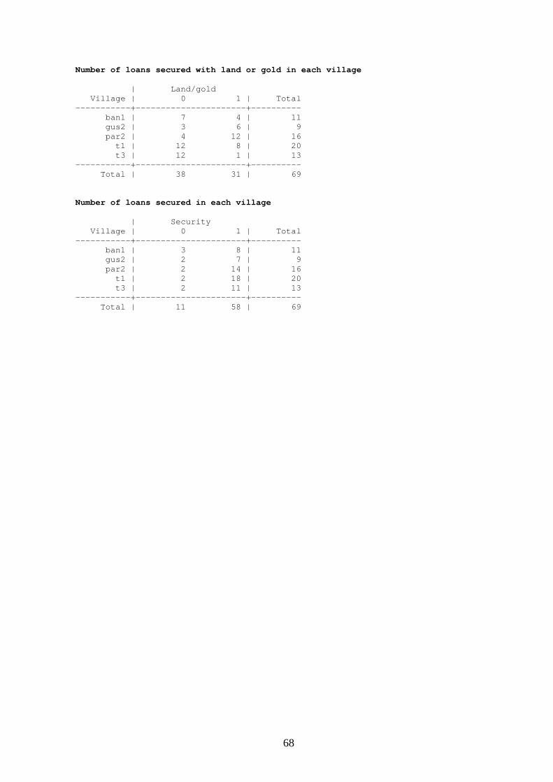
Number of loans secured with land or gold in each village | Land/gold Village | 0 1 | Total -----------+----------------------+---------- ban1 | 7 4 | 11 gus2 | 3 6 | 9 par2 | 4 12 | 16 t1 | 12 8 | 20 t3 | 12 1 | 13 -----------+----------------------+---------- Total | 38 31 | 69 Number of loans secured in each village | Security Village | 0 1 | Total -----------+----------------------+---------- ban1 | 3 8 | 11 gus2 | 2 7 | 9 par2 | 2 14 | 16 t1 | 2 18 | 20 t3 | 2 11 | 13 -----------+----------------------+---------- Total | 11 58 | 69

68

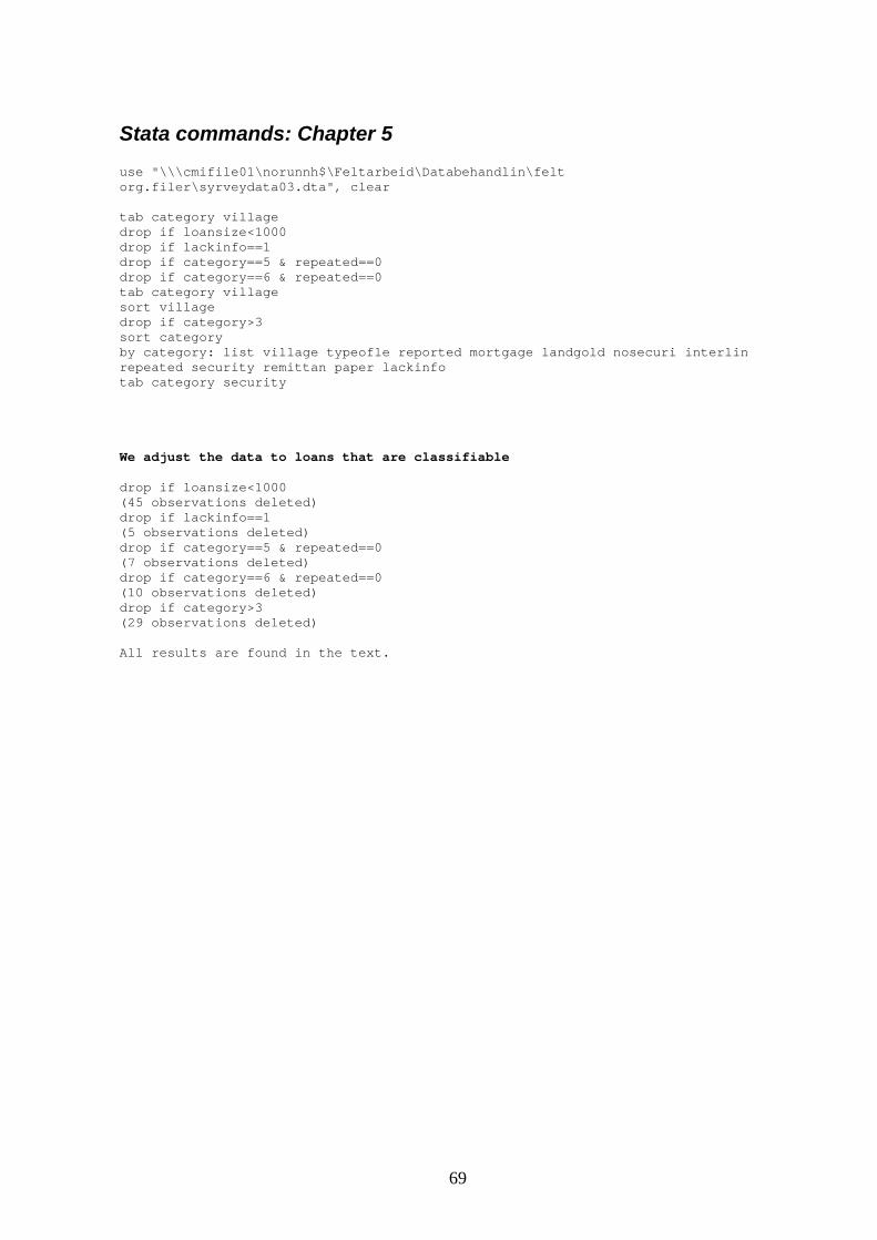
Stata commands: Chapter 5 use "\\\cmifile01\norunnh$\Feltarbeid\Databehandlin\felt org.filer\syrveydata03.dta", clear tab category village drop if loansize<1000 drop if lackinfo==1 drop if category==5 & repeated==0 drop if category==6 & repeated==0 tab category village sort village drop if category>3 sort category by category: list village typeofle reported mortgage landgold nosecuri interlin repeated security remittan paper lackinfo tab category security We adjust the data to loans that are classifiable drop if loansize<1000 (45 observations deleted) drop if lackinfo==1 (5 observations deleted) drop if category==5 & repeated==0 (7 observations deleted) drop if category==6 & repeated==0 (10 observations deleted) drop if category>3 (29 observations deleted) All results are found in the text.

69

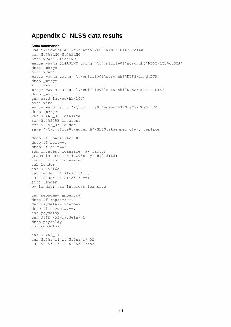
Appendix C: NLSS data results Stata commands use "\\\cmifile01\norunnh$\NLSS\RT065.DTA", clear gen S14A3LNO=S14A2LNO sort wwwhh S14A3LNO merge wwwhh S14A3LNO using "\\\cmifile01\norunnh$\NLSS\RT066.DTA" drop _merge sort wwwhh merge wwwhh using "\\\cmifile01\norunnh$\NLSS\land.DTA" drop _merge sort wwwhh merge wwwhh using "\\\cmifile01\norunnh$\NLSS\ethnic.DTA" drop _merge gen ward=int(wwwhh/100) sort ward merge ward using "\\\cmifile01\norunnh$\NLSS\RT090.DTA" drop _merge ren S14A2_08 loansize ren S14A209B interest ren S14A2_05 lender save "\\\cmifile01\norunnh$\NLSS\eksempel.dta", replace drop if loansize<1000 drop if belt==1 drop if belt==2 sum interest loansize [aw=factor] graph interest S14A206B, ylab(0(5)85) reg interest loansize tab lender tab S14A316A tab lender if S14A316A==5 tab lender if S14A316A==1 sort lender by lender: tab interest loansize gen repsome= amountpa drop if repsome==. gen paydelay= whenpay drop if paydelay==. tab paydelay gen diff=(52-paydelay>1) drop paydelay tab repdelay tab S14A3_17 tab S14A3_14 if S14A3_17>52 tab S14A3_15 if S14A3_17>52

70

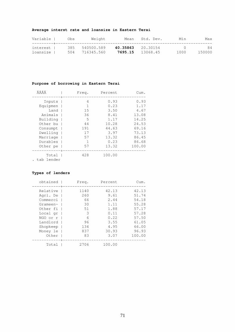
Average interst rate and loansize in Eastern Terai Variable | Obs Weight Mean Std. Dev. Min Max ---------+------------------------------------------------------------------ interest | 385 540500.589 40.35863 20.30154 0 84 loansize | 504 716345.560 7695.15 13068.45 1000 150000 Purpose of borrowing in Eastern Terai ÄÂÄÄ | Freq. Percent Cum. ------------+----------------------------------- Inputs | 4 0.93 0.93 Equipmen | 1 0.23 1.17 Land | 15 3.50 4.67 Animals | 36 8.41 13.08 Building | 5 1.17 14.25 Other bu | 44 10.28 24.53 Consumpt | 191 44.63 69.16 Dwelling | 17 3.97 73.13 Marriage | 57 13.32 86.45 Durables | 1 0.23 86.68 Other pe | 57 13.32 100.00 ------------+----------------------------------- Total | 428 100.00 . tab lender Types of lenders obtained | Freq. Percent Cum. ------------+----------------------------------- Relative | 1140 42.13 42.13 Agri. De | 260 9.61 51.74 Commerci | 66 2.44 54.18 Grameen- | 30 1.11 55.28 Other fi | 51 1.88 57.17 Local gr | 3 0.11 57.28 NGO or r | 6 0.22 57.50 Landlord | 96 3.55 61.05 Shopkeep | 134 4.95 66.00 Money le | 837 30.93 96.93 Other | 83 3.07 100.00 ------------+----------------------------------- Total | 2706 100.00

71

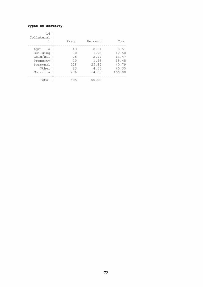
Types of security 16 | Collateral | 1 | Freq. Percent Cum. ------------+----------------------------------- Agri. la | 43 8.51 8.51 Building | 10 1.98 10.50 Gold/sil | 15 2.97 13.47 Property | 10 1.98 15.45 Personal | 128 25.35 40.79 Other | 23 4.55 45.35 No colla | 276 54.65 100.00 ------------+----------------------------------- Total | 505 100.00

72

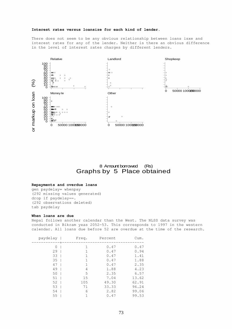
Interest rates versus loansize for each kind of lender. There does not seem to be any obvious relationship between loans isxe and interest rates for any of the lender. Neither is there an obvious difference in the level of interest rates charges by different lenders.

or

mar

kup o

n lo

an

(%

)

Graphs by 5 Place obtained 8 Amount borrowed (Rs)

Relative

0102030405060708090

100Landlord Shopkeep

0 50000 100000150000Money le

0 50000 1000001500000

102030405060708090

100Other

0 50000 100000150000

Repayments and overdue loans gen paydelay= whenpay (292 missing values generated) drop if paydelay==. (292 observations deleted) tab paydelay When loans are due Nepal follows another calendar than the West. The NLSS data survey was conducted in Bikram yeas 2052-53. This corresponds to 1997 in the western calendar. All loans due before 52 are overdue at the time of the research. paydelay | Freq. Percent Cum. ------------+----------------------------------- 0 | 1 0.47 0.47 29 | 1 0.47 0.94 33 | 1 0.47 1.41 35 | 1 0.47 1.88 47 | 1 0.47 2.35 49 | 4 1.88 4.23 50 | 5 2.35 6.57 51 | 15 7.04 13.62 52 | 105 49.30 62.91 53 | 71 33.33 96.24 54 | 6 2.82 99.06 55 | 1 0.47 99.53

73

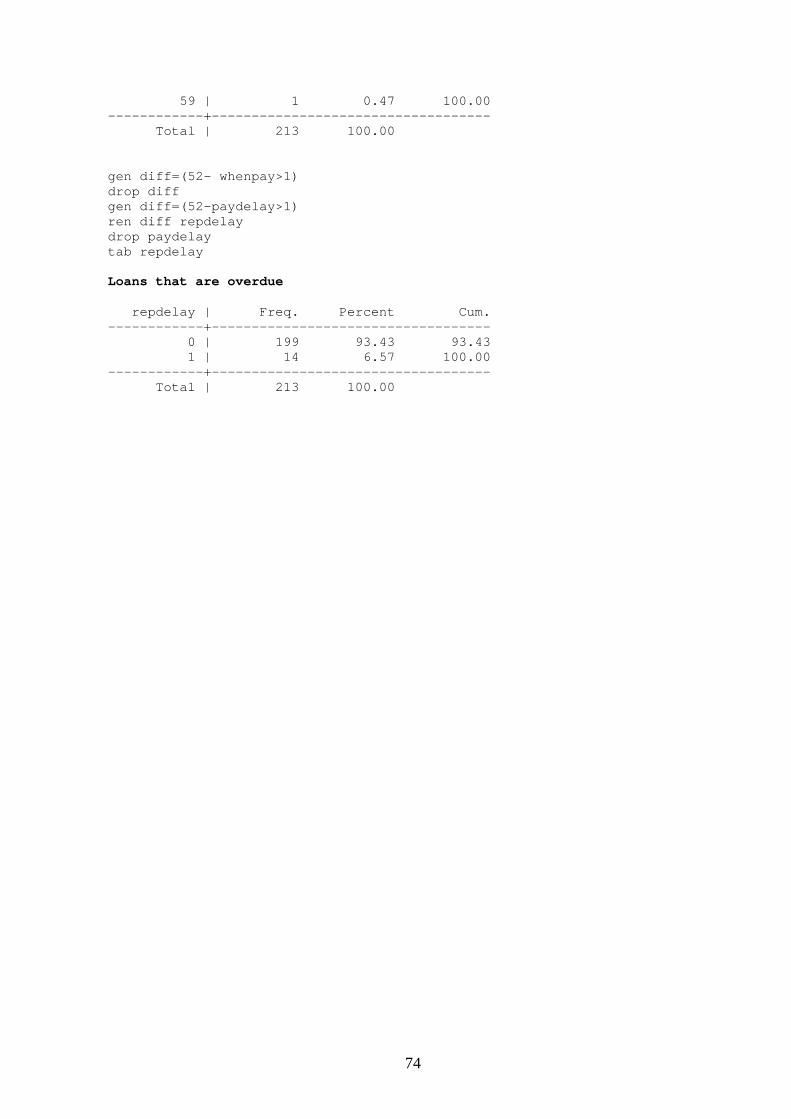
59 | 1 0.47 100.00 ------------+----------------------------------- Total | 213 100.00 gen diff=(52- whenpay>1) drop diff gen diff=(52-paydelay>1) ren diff repdelay drop paydelay tab repdelay Loans that are overdue repdelay | Freq. Percent Cum. ------------+----------------------------------- 0 | 199 93.43 93.43 1 | 14 6.57 100.00 ------------+----------------------------------- Total | 213 100.00

74