THE INFLUENCE OF THE CONDITIONS OF USE AND THE TYPE OF ...

57The Archives of Automotive Engineering – Archiwum Motoryzacji Vol. 85, No. 3, 2019

THE INFLUENCE OF THE CONDITIONS OF USE AND THE TYPE OF MODEL USED ON THE VERTICAL DYNAMIC

RESPONSES OF A CAR SUSPENSION

ZBYSZKO KLOCKIEWICZ1, GRZEGORZ ŚLASKI2, MIKOŁAJ SPADŁO3

Abstract

The article presents a study of the influence of vehicle’s conditions of use, such as road class, vehicle speed or its load, on its vertical dynamic responses. In the article only the kinematic excitations were analysed, as these are more common than the dynamic ones. The road profiles were artificially generated according to the ISO 8608 standard, which classifies roads based on power spectral density of excitations which they generate. Ride safety, ride comfort and fatigue strength indicators were computed. Ride safety was defined by the DLC – Dynamic Load Coefficient. Ride comfort was judged taking into consideration the recommendations from the ISO 2631 standard (which contains the information on vibration frequencies and their effect on human body, as well as the allowed exposure times to given vibrations) by calculating root mean square values of sprung mass accelerations for bandwidths defined in the standard. Load spectrums for the fatigue analysis were created using forces generated in a simulation as a basis and further research venues were proposed. Lastly conclusions were drawn from the results, that imply that linear models are sufficient for many standard applications on roads of acceptable quality, however the use of non-linear models is recommended in fatigue strength analysis regardless of conditions of use.

Keywords: car suspension; road excitation; dynamics simulation; vehicle models; fatigue strength

1. Introduction

Suspension systems in automobiles must fulfil many, often conflicting, requirements. The most commonly considered ones are the safety and ride comfort requirements, both really important for the user of the vehicle. Another important aspect, both for manufacturer and its user, is fatigue strength of the suspension elements. This one is related to geometrical dimensions of elements, which are limited in terms of space and mass used in a vehicle. Combination of these factors means that design or research process needs to take into consideration most of those requirements to be deemed viable.

1 Faculty of Transport Engineering, Poznan University of Technology, 3 Piotrowo Str., 60-965 Poznan, Polska, e-mail: [email protected]



58 The Archives of Automotive Engineering – Archiwum Motoryzacji Vol. 85, No. 3, 2019

The question arises now, how should this design or research process look like? In a mod-ern age, most of the work is at first done using Computer Aided Engineering software, which is understandable considering the high costs of prototype manufacturing. The au-thors of this article wanted to take a deeper look at the considerations one must make while doing simulations concerning the reliability of the results. Designers and researchers can use many different vehicle or road models, both linear and non-linear. Those models are described by their structures and many parameters, some of which are not constant in time and can change depending on the conditions of use, such as the vehicle’s velocity or its load, i.e. how many passengers/cargo is being transported and how it is distributed. All of the aforementioned factors directly or indirectly contribute to the way the vehicle model responds to inputs in the form of excitations.

To run a computer simulation one must first possess a vehicle model as well as a road, or more broadly speaking, excitation model. There are many different kinds of these models of varying degree of complication. At first researchers analysed mainly simple linear quarter-car models, which can be found in [13], [19], [25]. These models are still used in newer publications, for example in [4] or [5]. As the years went by, more and more research and simulations were made using non-linear models, especially in the last decade [20], [30]. Linear half-car models have been used for a long time as well, and can be found in [19], but also newer publications like [14], [18], [23]. Non-linear half car models can be found for example in [15], dating as far back as 1985. In [19] and [10] a lin-ear full-car model can be found. Work [26] describes all three kinds of vehicle models, with the addition of non-linear variants for quarter- and half-car models. When it comes to road models and their generation, most publications began by analysing periodical excitations consisting of one or more sine waves [19], [25], followed by the gradual shift towards random profiles described by statistical values [3], [6], [11]. After the introduc-tion of IRI in 1986 researchers tried modelling their profiles, so that they possessed given IRI values [14], [12]. In the next decade, when ISO 8608 standard was released, many researchers found it better suited for modelling different road types, that is why so many modern road profiles are generated according to this standard, as can be seen for exam-ple in [6], [18], [21], [30].


Fig. 1. Road classification according to ISO 8608 standard. The basic spatial frequency value is marked in red

The excitations that vehicles are subjected to can be generally divided into two subcat-egories – determined and random excitations. The first ones are profiles, which can be described using mathematical functions or their combinations. Random functions on the other hand are generated randomly, with often only statistical description of given pa-rameters available. One example of random profiles are profiles created based on power spectral density (PSD) of excitations (specifically – the height of those excitations) ac-cording to ISO 8608 – Figure 1. The ISO standard divides all profiles into categories based on PSD (vertical axis) as the function of spatial frequency of excitation (horizontal axis), starting with class A, which describes very good surfaces like runways and highways, and decreasing in quality with each subsequent letter of the alphabet. The consequent lines represent the borders between each road class. Profiles generated in accordance with that standard were used in simulation as a source of kinematic excitations to the models in the article. PSD is calculated using the following formula:

The Archives of Automotive Engineering – Archiwum Motoryzacji

randomly, with often only statistical description of given parameters available. One example of random profiles are profiles created based on power spectral density (PSD) of excitations (specifically – the height of those excitations) according to ISO 8608 – Figure 1. The ISO standard divides all profiles into categories based on PSD (vertical axis) as the function of spatial frequency of excitation (horizontal axis), starting with class A, which describes very good surfaces like runways and highways, and decreasing in quality with each subsequent letter of the alphabet. The consequent lines represent the borders between each road class. Profiles generated in accordance with that standard were used in simulation as a source of kinematic excitations to the models in the article. PSD is calculated using the following formula:

𝜙𝜙ℎ(𝛺𝛺) = 𝜙𝜙ℎ(𝛺𝛺0) ∙ (𝛺𝛺𝛺𝛺0)−2

(1)

Where:

• 𝜙𝜙ℎ(𝛺𝛺) – power spectral density of excitations as a function of spatial frequency 𝛺𝛺, [m3],

• 𝜙𝜙ℎ(𝛺𝛺0) – reference power spectral density for a basic spatial frequency 𝛺𝛺0, [m3] (border values for different road classes can be found for example in [29]),

• 𝛺𝛺 – spatial frequency, [rad/m], • 𝛺𝛺0 – basic spatial frequency, equal to 1 rad/m.

For temporal frequency, the equation would look as such:

𝜙𝜙ℎ(𝑛𝑛) = 𝜙𝜙ℎ(𝑛𝑛0) ∙ (𝑛𝑛𝑛𝑛0)−2

(2)

Where:

• 𝜙𝜙ℎ(𝑛𝑛) – power spectral density of excitations as a function of spatial frequency 𝑛𝑛, [m3], • 𝜙𝜙ℎ(𝑛𝑛0) – reference power spectral density for a basic spatial frequency 𝑛𝑛0, [m3] (border values

for different road classes can be found for example in [29]), • 𝑛𝑛 – spatial frequency, [cycles/m], • 𝑛𝑛0 – basic spatial frequency, equal to 0.1 cycles/m.

2. Models tested in simulation

During the simulation models for the suspension system and the kinematic excitations were used. The suspension models differed in terms of structure (one was quarter-car model, while the other was half car model). The elements of the suspension themselves were also modelled in two different ways – firstly as a simple linear functions, secondly as full characteristics describing forces in those element as functions of displacement (springs) or displacement’s velocity (dampers). Kinematic excitations were modelled using procedures based on [21], which discusses the generation of road profiles according to classes defined in ISO 8608 standard. To obtain kinematic excitation from road profile, the use of tire model is normally needed, in the presented case the tire model was replaced by defining the shortest existing profile wavelength to be 0.2 m, which is the typical passenger car tire contact length.

2.1 Vehicle models

There were two different vehicle models used in simulations, both of which had linear and non-linear variants. The first was a quarter-car model (Figure 2a) consisting of two masses – sprung one labelled MQ and unsprung one, m. Both of them have only 1 DOF – movement in the vertical direction. They interact with each other via spring with stiffness kM and damper with damping coefficient cM, which depending on the model are either simple coefficients or (in the non-linear models) are modelled in the


Where:

• ϕh(Ω) – power spectral density of excitations as a function of spatial frequency Ω, [m3],

• ϕh (Ω0) – reference power spectral density for a basic spatial frequency Ω0, [m3] (border values for different road classes can be found for example in [29]),

• Ω – spatial frequency, [rad/m],

• Ω0 – basic spatial frequency, equal to 1 rad/m.



randomly, with often only statistical description of given parameters available. One example of random profiles are profiles created based on power spectral density (PSD) of excitations (specifically – the height of those excitations) according to ISO 8608 – Figure 1. The ISO standard divides all profiles into categories based on PSD (vertical axis) as the function of spatial frequency of excitation (horizontal axis), starting with class A, which describes very good surfaces like runways and highways, and decreasing in quality with each subsequent letter of the alphabet. The consequent lines represent the borders between each road class. Profiles generated in accordance with that standard were used in simulation as a source of kinematic excitations to the models in the article. PSD is calculated using the following formula:

𝜙𝜙ℎ(𝛺𝛺) = 𝜙𝜙ℎ(𝛺𝛺0) ∙ (𝛺𝛺𝛺𝛺0)−2

(1)

Where:

• 𝜙𝜙ℎ(𝛺𝛺) – power spectral density of excitations as a function of spatial frequency 𝛺𝛺, [m3],

• 𝜙𝜙ℎ(𝛺𝛺0) – reference power spectral density for a basic spatial frequency 𝛺𝛺0, [m3] (border values for different road classes can be found for example in [29]),

• 𝛺𝛺 – spatial frequency, [rad/m], • 𝛺𝛺0 – basic spatial frequency, equal to 1 rad/m.


𝜙𝜙ℎ(𝑛𝑛) = 𝜙𝜙ℎ(𝑛𝑛0) ∙ (𝑛𝑛𝑛𝑛0)−2

(2)

Where:

• 𝜙𝜙ℎ(𝑛𝑛) – power spectral density of excitations as a function of spatial frequency 𝑛𝑛, [m3], • 𝜙𝜙ℎ(𝑛𝑛0) – reference power spectral density for a basic spatial frequency 𝑛𝑛0, [m3] (border values

for different road classes can be found for example in [29]), • 𝑛𝑛 – spatial frequency, [cycles/m], • 𝑛𝑛0 – basic spatial frequency, equal to 0.1 cycles/m.


During the simulation models for the suspension system and the kinematic excitations were used. The suspension models differed in terms of structure (one was quarter-car model, while the other was half car model). The elements of the suspension themselves were also modelled in two different ways – firstly as a simple linear functions, secondly as full characteristics describing forces in those element as functions of displacement (springs) or displacement’s velocity (dampers). Kinematic excitations were modelled using procedures based on [21], which discusses the generation of road profiles according to classes defined in ISO 8608 standard. To obtain kinematic excitation from road profile, the use of tire model is normally needed, in the presented case the tire model was replaced by defining the shortest existing profile wavelength to be 0.2 m, which is the typical passenger car tire contact length.

2.1 Vehicle models

There were two different vehicle models used in simulations, both of which had linear and non-linear variants. The first was a quarter-car model (Figure 2a) consisting of two masses – sprung one labelled MQ and unsprung one, m. Both of them have only 1 DOF – movement in the vertical direction. They interact with each other via spring with stiffness kM and damper with damping coefficient cM, which depending on the model are either simple coefficients or (in the non-linear models) are modelled in the

Where:

• ϕh (n) – power spectral density of excitations as a function of spatial frequency n, [m3],

• ϕh (n0) – reference power spectral density for a basic spatial frequency n0, [m3] (border values for different road classes can be found for example in [29]),

• n – spatial frequency, [cycles/m],

• n0 – basic spatial frequency, equal to 0.1 cycles/m.


During the simulation models for the suspension system and the kinematic excitations were used. The suspension models differed in terms of structure (one was quarter-car model, while the other was half car model). The elements of the suspension themselves were also modelled in two different ways – firstly as a simple linear functions, secondly as full characteristics describing forces in those element as functions of displacement (springs) or displacement’s velocity (dampers).

Kinematic excitations were modelled using procedures based on [21], which discusses the generation of road profiles according to classes defined in ISO 8608 standard. To ob-tain kinematic excitation from road profile, the use of tire model is normally needed, in the presented case the tire model was replaced by defining the shortest existing profile wave-length to be 0.2 m, which is the typical passenger car tire contact length.

2.1 Vehicle models

There were two different vehicle models used in simulations, both of which had linear and non-linear variants. The first was a quarter-car model (Figure 2a) consisting of two masses – sprung one labelled MQ and unsprung one, m. Both of them have only 1 DOF – movement in the vertical direction. They interact with each other via spring with stiffness kM and damper with damping coefficient cM, which depending on the model are either simple co-efficients or (in the non-linear models) are modelled in the form of lookup tables containing spring and damper characteristics. Linear model parameters of stiffness of front and rear suspensions are estimated on the base of springs characteristics in static load area and


kinematic ratios for front and rear suspensions. Linear model parameters for damping of front and rear suspension were estimated as the average value for the deflection’s veloc-ity range between 0.2 m/s and -0.2 m/s. In this research the parameters for the quarter car model were set as the ones for the rear suspension.

The tire forces are modelled using stiffness km and damping cm coefficients. Non-linear model has tire forces’ values switched to zero whenever the tire deflection reaches posi-tive values, as it means the tire has lost contact with the road profile.

Fig. 2. a) Quarter- and b) half-car models used in simulations

The half-car model, which is presented in Figure 2b, is quite similar to the quarter-car mod-el. The differences are that the sprung mass is defined not only by its mass MH, but also by its moment of inertia I around the horizontal axis. There are two unsprung masses, front one (values with index “f”) and rear one (index “r”). They consist of the same elements, as the ones in quarter-car model. Both of them affect the sprung mass not in its centre of mass, but instead of in points with distances from the centre given by lengths lf and lr.

2.2 Characteristics of springs and dampers

The characteristics of springs and shock absorbers were acquired experimentally (de-scribed in [24]), with minor corrections made to them, to model suspension stiffness and damping instead of real spring and damper parameters. These characteristics are shown in Figure 3. All the characteristics already take into account the kinematic ratios needed to compute the forces actually acting on suspension elements. For both front spring and damper the ratio was 0.94, for the rear spring it was 1.05 and for the rear damper 0.68.


Fig. 3. Damper and spring characteristics used in models

The linear and non-linear quarter car model tested during simulation used characteristics from the rear axle of modelled car. The only modification from the experimental data gath-ered in [24] of the damper characteristics’ was the inclusion of kinematic ratio. The springs had to undergo more serious modifications, especially the rear spring characteristic, as the experimental data was that of a spring dismounted from its socket in the rear torsion beam. This means that the effects of the bump stop were omitted in the original spring test and had to be manually added. The suspension deflection values, at which the bump stop starts to work were determined experimentally. Because the spring normally is mounted slightly compressed, the characteristics had to also include that fact, so the whole dia-gram was moved down by subtracting the static force value from the characteristic. On the other side of the spectrum, when the spring is fully compressed, the steep increase in force value was added, simulating the fact that in order to compress suspension any further, the suspension parts would have to be deformed.

Another difference between the linear and non-linear models was the model of the tire forces. The linear models allowed for both compression and extension of the tire, with the latter causing the appearance of forces that pulled the wheel to the ground. That of course does not happen in real conditions of use, so in the non-linear models the forces in the tire are set to zero whenever the tire deflection is positive in value.

The most important parameter values for both model are presented in Table 1 and Table 2. These values model the vehicle described in [24]. The vehicle is Opel Astra III estate, which is a typical C-segment passenger car from the most common vehicle segment in the European market, if you include SUVs [2].


Tab. 1. Characteristic parameters for the quarter-car model (rear suspension)

Parameter Symbol Value

Unsprung mass m 35 [kg]

Sprung mass MQ 230÷400 [kg]

Suspension stiffness* kM 20800 [N/m]

Suspension damping* cM 2050 [Ns/m]

Tire stiffness km 140000 [N/m]

Tire damping cm 230 [Ns/m]

* - only in linear model

Tab. 2. Characteristic values for the half-car model

Parameter Symbol Value

Unsprung mass front (rear) mf (mr) 40 (35) [kg]

Sprung mass (for half of the car) MH 630÷845 [kg]

Moment of inertia (for half of the car) I 900 [kg·m2]

Suspension stiffness front (rear)* kMf (kMr) 19300 (20800) [N/m]

Suspension damping front (rear)* cMf (cMr) 2100 (2050) [Ns/m]

Tire stiffness front (rear) kmf(kmr) 160000 (140000) [N/m]

Tire damping front (rear) cmf (cmr) 230 (230) [Ns/m]

Wheel base wb 2.703 [m]

Distance from the front axle to the centre of mass

lf 1.030÷1.280 [m]

Distance from the rear axle to the centre of mass

lr 1.424÷1.673 [m]


2.3 Road model

The vehicle model was tested with excitations from four different road irregularity profiles, belonging to classes A to D defined in ISO 8608 standard. The road profiles were gener-ated using method described in [22]. The Matlab function that generated profiles used geometric mean values of the vertical displacement power spectral density for each road class as they are given in ISO 8608 [21]. Road waviness was constant and set to 2. The vertical displacement PSD was then calculated for a range of angular spatial frequencies with its borders defined by set longest (90 m) and shortest (0.2 m) wavelengths. These wavelengths were chosen as the tire filtrates unevennesses shorter than 0.2 m, as that is the average contact length of tire-pavement pair for passenger cars. Unevennesses longer than 90 m would recquire a very high speed of around 180 km/h to be noticable, which is rarely accomplished on public roads due to speed limits and safety reasons. Randomly


distributed phase shift was also calculated and both of these were later used in an equa-tion that created a number or profiles for every frequency, that were ultimately summed together to create road profile from a chosen road class.

3. Criteria for dynamic responses’ evaluation

To find a measurable way to establish differences between models being examined, the authors proposed following criteria for chosen suspension responses: ride safety, ride comfort and fatigue strength analysis.

3.1 Safety criteria

The ride safety was judged based on an index called dynamic load coefficient (DLC) [21]. The DLC is calculated by dividing the root mean square of the dynamic tire force Fdyn (de-fined as the difference between momentary and static force values) by the static tire force Fstat, as seen in equation (3). Tire force is calculated in a model as a sum of stiffness and damping forces of a tire.


Tab. 2. Characteristic values for the half-car model Parameter Symbol Value Unsprung mass front (rear) mf (mr) 40 (35) [kg] Sprung mass (for half of the car) MH 630÷845 [kg] Moment of inertia (for half of the car) I 900 [kg·m2] Suspension stiffness front (rear)* kMf (kMr) 19300 (20800) [N/m] Suspension damping front (rear)* cMf (cMr) 2100 (2050) [Ns/m] Tire stiffness front (rear) kmf(kmr) 160000 (140000) [N/m] Tire damping front (rear) cmf (cmr) 230 (230) [Ns/m] Wheel base wb 2.703 [m] Distance from the front axle to the centre of mass lf 1.030÷1.280 [m] Distance from the rear axle to the centre of mass lr 1.424÷1.673 [m]


2.3 Road model

The vehicle model was tested with excitations from four different road irregularity profiles, belonging to classes A to D defined in ISO 8608 standard. The road profiles were generated using method described in [22]. The Matlab function that generated profiles used geometric mean values of the vertical displacement power spectral density for each road class as they are given in ISO 8608 [21]. Road waviness was constant and set to 2. The vertical displacement PSD was then calculated for a range of angular spatial frequencies with its borders defined by set longest (90 m) and shortest (0.2 m) wavelengths. These wavelengths were chosen as the tire filtrates unevennesses shorter than 0.2 m, as that is the average contact length of tire-pavement pair for passenger cars. Unevennesses longer than 90 m would recquire a very high speed of around 180 km/h to be noticable, which is rarely accomplished on public roads due to speed limits and safety reasons. Randomly distributed phase shift was also calculated and both of these were later used in an equation that created a number or profiles for every frequency, that were ultimately summed together to create road profile from a chosen road class.

3. Criteria for dynamic responses’ evaluation

To find a measurable way to establish differences between models being examined, the authors proposed following criteria for chosen suspension responses: ride safety, ride comfort and fatigue strength analysis.

3.1 Safety criteria

The ride safety was judged based on an index called dynamic load coefficient (DLC) [21]. The DLC is calculated by dividing the root mean square of the dynamic tire force 𝐹𝐹𝑑𝑑𝑑𝑑𝑑𝑑 (defined as the difference between momentary and static force values) by the static tire force 𝐹𝐹𝑠𝑠𝑠𝑠𝑠𝑠𝑠𝑠, as seen in equation (3). Tire force is calculated in a model as a sum of stiffness and damping forces of a tire.

𝐷𝐷𝐷𝐷𝐷𝐷 =𝑅𝑅𝑅𝑅𝑅𝑅(𝐹𝐹𝑑𝑑𝑑𝑑𝑑𝑑)

𝐹𝐹𝑠𝑠𝑠𝑠𝑠𝑠𝑠𝑠 (3)

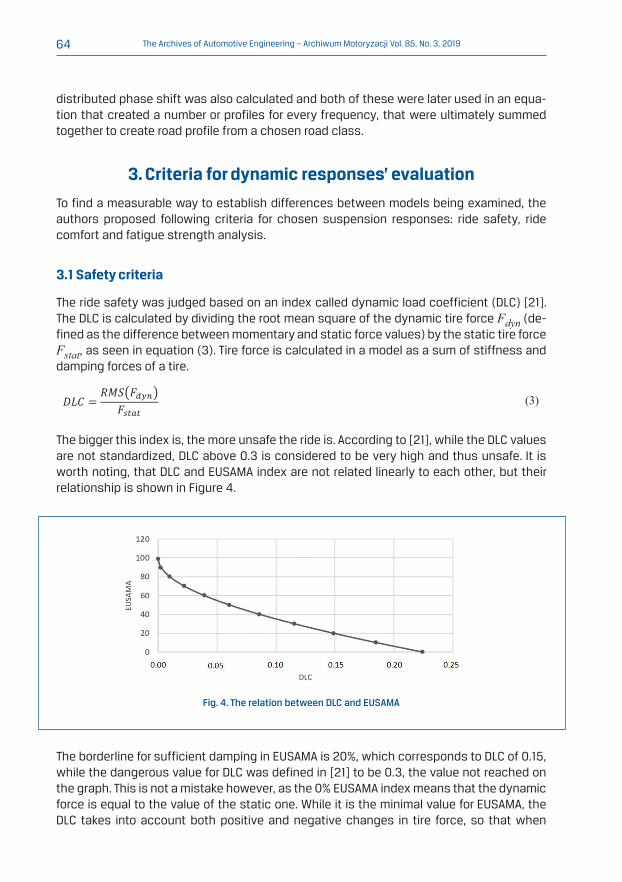
The bigger this index is, the more unsafe the ride is. According to [21], while the DLC values are not standardized, DLC above 0.3 is considered to be very high and thus unsafe. It is worth noting, that DLC and EUSAMA index are not related linearly to each other, but their relationship is shown in Figure 4. The bigger this index is, the more unsafe the ride is. According to [21], while the DLC values are not standardized, DLC above 0.3 is considered to be very high and thus unsafe. It is worth noting, that DLC and EUSAMA index are not related linearly to each other, but their relationship is shown in Figure 4.

Fig. 4. The relation between DLC and EUSAMA

The borderline for sufficient damping in EUSAMA is 20%, which corresponds to DLC of 0.15, while the dangerous value for DLC was defined in [21] to be 0.3, the value not reached on the graph. This is not a mistake however, as the 0% EUSAMA index means that the dynamic force is equal to the value of the static one. While it is the minimal value for EUSAMA, the DLC takes into account both positive and negative changes in tire force, so that when


its value increases significantly, the DLC can assume values for non-existent negative EUSAMA percentages.

3.2 Comfort criteria

Due to simplicity of used models (the lack of seat model) sprung mass accelerations were calculated and used in order to establish the comfort levels of every simulated ride. The time domain signals were subjected to frequency analysis, with signal components of dif-fering frequencies being distinguished. The frequency bands were taken from the ISO 2631 standard and RMS values for accelerations were calculated for those frequency bands as ride comfort indexes. These values were then compared with the recommendations from the ISO 2631 standard regarding to the exposure limit (EL), fatigue decreased profi-ciency (FDP) boundary and reduced comfort boundary (RCB) [1] for a given time period of exposure to vibration – in the case of this paper it was 8 h exposure (Figure 5). It is worth noting, that in this paper the comparison with the chosen limits is not as important as the comparison of calculated values for different models and conditions of use. The values on the horizontal axis are the mid points of consecutive 1/3 octave bands.

Fig. 5. Limits of acceptable accelerations according to ISO 2631 [9]. The horizontal axis values are the mid points of 1/3 octave bands, the vertical axis shows the RMS of sprung mass accelerations

3.3 Fatigue strength criteria

The load-times histories obtained as a result of the simulations were subjected to further processing to estimate the impact of the implementation of the non-linear suspension model on the fatigue aspects. The procedure of fatigue assessment of car component on the base of load time history is illustrated in Figure 6. In this research load is defined as the sum of forces in the suspension - sum of spring and damper forces acting on vehicle body at upper suspension mount and on suspension elements on lower mount. At this research stage this is an acceptable assumption due to simplified models used for the research.

The first stage of fatigue assessment after acquiring load-time histories (from simulation or experimental tests) is the analysis of dynamic responses of the vehicle body or a sus-pension structure under investigation with the use of finite element method, which results


in obtaining information on stresses caused by acquired loads. In a further step, random stresses are transformed using the Rainflow counting method to a set of cycles that are used in the determination of fatigue characteristics, i.e. stress cycles of a given mean and amplitude value and their number that causes given damage. In the final stage, the esti-mation of durability is carried out using for example 1-parameter characteristics like S-N (amplitude of stress vs number of cycles diagram) curves or 2-parameter characteristics like Goodman-Smith or Haigh graphs etc. (amplitude and mean value of stress vs number of cycles diagram). More detailed information about each step can be found in the litera-ture of the subject, for example in [7], [8], [17], [28].

Due to simplicity of models tested in this research it was not possible to calculate stresses of body or suspension structure. Assuming linear relation between loads and stresses au-thors decided to analyse changes in a load spectrum instead of stresses spectrum as an information allowing to estimate qualitive changes in a fatigue strength and the criteria chosen for that evaluation was the number of cycles, which is commonly used in fatigue strength analysis for this purpose.

Fig. 6. Procedure of fatigue assessment of car component

The paper describes the results of analyses that omitted the FEM research stage and im-plemented the Rainflow method directly to the load-time histories. This treatment allowed to eliminate the influence of the dynamic properties of the structure on the stress values, so that ratiocination is clearer. The analyses were limited to observing the effects of using


Rainflow, without further calculation of fatigue. The obtained result is a set of amplitudes and mean values of loads instead of stresses. With these results and linear relation be-tween loads and stresses, it is possible to estimate the impact of the implementation of the non-linear suspension model on the fatigue aspects, as it is being assumed that there is a linear relation between loads and stresses. This simplified method is shown in Figure 7.

Fig. 7. Simplified procedure of estimation of load spectra influence on fatigue strength

4. Description of the experiment

The experiment took into account variability of three different conditions of use, which change in real life – road class, vehicle velocity and its load. All of the simulation runs were made using all four types of models: linear and non-linear as well as quarter- and half-car. The changing conditions of use were as follows:

• road profiles ranging from class A roads (good quality highways, airstrips runways) through B (express ways of acceptable quality) and C (standard to low quality roads, often connecting cities or running through them) to D class roads, which are usually rural roads or cobblestone streets – Figure 8;

Fig. 8. A comparison of generated road profiles of classes A to D. The differences between maximum and minimum profile height values are: A – 0.022 m, B – 0.026 m, C – 0.087 m, D – 0.157 m.


• vehicle velocity ranging from the highest speed (vmax) taken around values permitted by law on roads classes A and B (respectively: 40 m/s and 30 m/s) or the highest speed for which the safety requirement in [21] is met for road classes C (20 m/s) and D (5 m/s) to the lowest speed simulated (vmin), which was 50 to 70% lower than the highest one. The third velocity (v2) was set to be in the middle of the two previously mentioned ve-locities (Table 3);

Tab. 3. Vehicle speed charts depending on a road class used

Road class

Velocity A B C D

vmax [m/s]/[km/h] 40/108 30/108 20/72 5/18

v2 [m/s]/[km/h] 30/108 22/79 12/43 3/11

vmin [m/s]/[km/h] 20/72 15/54 5/18 1/4

• vehicle load ranging from a vehicle with only driver sitting inside to 5 passengers with 50 kg of luggage in the trunk. The other variants tested were 3 passengers and 5 pas-sengers without luggage (Table 4). The sprung mass values were taken from [27] (Figure 9) and calculated as a mean of left and right wheel values.

Tab. 4. Sprung mass of front, rear (used in quarter car model) and the sum of them (equal to the sprung mass in half car model)

Front sprung mass [kg]

Rear sprung mass [kg]

Sum [kg]

1 passenger 390 240 630

3 passengers 430 295 725

5 passengers 445 350 795

5 pas. + luggage 445 400 845

Fig. 9. Changes in sprung mass values as a function of changing vehicle load [27]. Red circles indicate cases that were used in simulation


The experiments were carried out in Matlab Simulink using vehicle models created by the authors of the article, with simulation time set to 10 s with a timestep of 0.001 s. The cal-culated values were:

• acceleration of sprung mass - accM,

• total force in suspension elements - ∑Fsusp,

• total force in the tire - ∑Ftire,

• suspension deflection - ∆z.

5. Results’ analysis

After all the simulation cases were run and the time-domain signals were used to calculate indicators for ride comfort, ride safety and fatigue strength, the analysis of those indica-tors was conducted. The number of tests was very high, which is why it was decided to narrow down their number to those, in which the non-linear suspension work range was exceeded frequently.

This lead researchers to create a preliminary system of selecting cases worth further anal-ysis on the basis of suspension deflection – whether or not the deflection reached the non-linear zone and if so, what percentage of the samples was in this zone. To do that, spring characteristics were compared with cumulative frequency of deflections of subse-quent experiments and the percentage of those in the non-linear range was read (Figure 10). If less than 2% of the deflections were in the non-linear zone, it was determined that those cases do not need detailed examination. The results are shown in Table 5.

Tab. 5. Tables showing cases, where suspension deflection entered non-linear range. Red – both rear and front suspension, yellow – only front suspension, green – work only in linear range.

Road class A B C D

Speed [m/s] 40 30 20 30 22 15 20 12 5 5 3 1

5+lug.

5

3

1


Fig. 10. The example of determining the percentage of deflections in the non-linear range for a C class road, v =20 m/s and 3 passengers on board

Based on that method and the results gathered in Table 5 one can observe that on bad quality roads of classes C and D, models work in non-linear range for almost every load-speed combination, with the exception of 1 passenger case or 3 passengers with the lowest simulated velocity. In the B class road the non-linear range is reached, when the number of passengers reaches 5, while in the A class there is no load-speed combination, in which the percentage of deflections in the non-linear range exceeds 2%. This lead the researchers to narrow the amount of cases analysed. In the following paper, the results for the worst possible scenarios for every road class are presented, which means 5 passen-gers with luggage and maximum velocity for a given road class. This includes also roads from class A, which theoretically should not exhibit differences between linear and non-linear models based on previous assumptions. It was done for the sake of completeness and to make sure the chosen method for narrowing research scope was correct.

To ascertain, whether the dampers worked in a linear range in the same cases, the same procedure was applied to deflection’s speeds’ results (Figure 11). The range which can be linearly modelled with decent accuracy was established to be (-0.2 to 0.2) m/s. On the A class road, even a fully loaded car stayed in this range over 99% of the time. The same cannot be said regarding to roads from classes B to D – in those cases the percentage crosses to non-linear range was between 8% for the B class road to 34% for the D class road. Those number dropped with decreasing number of passengers on board or vehicle velocity, falling in line with the results presented in Table 5.


Fig. 11. Front damper characteristics for a half-car model with the deflection's speeds' results for 5 passengers with luggage and the highest tested velocity on a given road class

5.1 Ride safety results

The DLC comparison for different road classes is presented in Figure 12. Every chart is made for the maximum speed the simulated car was travelling with on a given road: from 40 m/s on the A class road to 5 m/s for the D class road. Each chart shows the changes in DLC for the increase in the number of passengers, which usually causes a drop in the DLC value. It is caused by the fact, that the denominator becomes greater faster than the numerator in equation (3). It is especially visible for the rear suspension, as the changes in sprung mass, and in turn in tire static force there are bigger than for front axle – see Figure 9.

Linear and non-linear model comparison

The percentage values of differences between non-linear and linear models were calcu-lated in reference to linear model values. For all instances the differences between quarter car models are slight, not exceeding 5% (4.8% being the biggest difference for A class road at 40 m/s and 1 passenger), as is shown in Figure 12.

Half car models however differ more significantly, with the DLC of non-linear models be-ing usually higher. The extent of that difference varies and is much more pronounced in


the front suspension. The non-linear model always yields higher DLC values, even if by as little as 1.5%. In the case of D class road and 5 passengers with luggage the difference reaches up to 29% higher values between non-linear and linear half car models. This might be a result of the mass distribution in the half car model, in which the front is more heavily loaded, giving the rear lower static tire force value, which in turn leads to a higher calcu-lated DLC. This explains why the difference between non-linear and linear front suspension DLC is the smallest for the case with 1 passenger, where the front suspension deflection is furthest from entering non-linear range.

Smaller differences in DLC values are observed between non-linear and the linear half car’s rear suspension and they do not show any particular trend. The DLC value for non-linear model is higher than the DLC values for linear model for road classes A and D, and lower for classes B and C. The difference is the biggest, when the load has the lowest value, which suggests this difference comes from the fact that front suspension’s movements do not limit the rear’s movements, which in turn generates bigger force oscillations – for example, for C class road and 1 passenger the DLC value of non-linear model is smaller by up to 0.02 (9.1%) from linear model DLC value. This can be observed in both B and C class roads, hav-ing respectively 5.4% and 9.1% lower DLC values for rear suspension for half car model with 1 passenger, while roads from classes A and D display a slightly bigger DLC values in favour of non-linear model’s DLC of about 2%.

The quarter to half car model comparison

There are also noticeable differences between quarter and half car models. The differences between half car and quarter car models were calculated in reference to quarter car model. The quarter car models generally have DLC higher than the front suspension in the half car model, but lower than the rear suspension – Figure 12. This probably has to do with the mentioned previously difference between static loads for the front and rear in half car model. This difference is not universal – with the increase of the number of passengers on board the DLC values for the front suspension get closer to those from quarter car models, being slightly higher (7.4% for the D class road and 9.7% for A class road) for a fully loaded car. The front suspension’s DLC is lower by up to 23% for 1 passenger case and it gets high-er by 25% for 5 passengers with luggage (for the linear half car model – for the non-linear one it is 38%). It should also be noted that quarter car model was modelled after the rear suspension, so it is expected that the results will be closer to those of a rear suspension of half car model.


Fig. 12. DLC comparison for different road classes and loads

Comparison for different loads

The differences for increasing weight were referred to 1 passenger case. The results show (Figure 12) that with the increase in the number of passengers, the DLC values get lower and lower for almost every model (quarter or half car and non-linear or linear models) and road class combination, with the only exception being non-linear front suspension of a half car model on the D class road, where the DLC grows slightly (7.9% increase from 1 pas-senger to 5 passengers). It should be noted, that the changes in DLC values are the lowest for half car front suspension having DLC values for 5 passengers between 3.6% and 11.6% lower than for the 1 passenger. For the same change of load the quarter car model experi-ences increase in DLC value of (28-29)% and the rear suspension’s DLC of half car model in-creases by 25% to 29%. This is due to the mass distribution and the fact, that front doesn’t change as much as the rear in the regard of sprung mass increase. Coupled with the fact, that on the D class road there are many irregularities which cause the suspension to enter non-linear range and the DLC increase for those roads is to be expected.

Comparison for different speeds

The calculations for the speed changes were carried out having DLC value for the high-est speed as the reference value. The difference in DLC with vehicle’s speed is the most noticeable in the case of the D class road, where decreasing speed from 5 m/s to 1 m/s (80% reduction) causes a 67% reduction in DLC value for rear suspension in half car model, both linear and non-linear – Figure 13. At the same time, front suspension’s DLC changes by 35%. The change for C class road on the other hand is best seen in front suspension


– being lower by 55%, when the speed changes from 20 m/s to 5 m/s (75% reduction). The smallest changes are seen for road classes A and B – with their maximum reduction in speed of 50%, the DLC dropped by at most 32%. The decrease in vehicle’s speed cause the DLC to drop by a lower percentage, than the percentage in which the speed changed – for example, for an A class road changing the speed by 50% form 40 m/s to 20 m/s caused the DLC to decrease by about 31% for all tested vehicle models. In most cases the drop in percentage was slightly (0.5% to 1%) lower for non-linear models.

Fig. 13. Comparison of DLC for different vehicle models on roads from class A to D and changing vehicle velocity

5.2 Ride comfort results

The comparison of ride comfort indexes between the models was carried out similarly to the comparisons described in chapter 5.1 with quarter car models being the reference. The case presented in Figure 14 was chosen as typical example of how the charts for comfort comparison look like.

Linear and non-linear model comparison

In the case of linear and non-linear models comparison the linear model values were used as the reference values – Figure 15.

The linear and non-linear quarter car models yield similar results for low frequencies up to 2 Hz, higher by up to 14% in favour of non-linear model. Similar dependency is observed for high frequencies over 20 Hz – the non-linear models have values higher than the linear


ones, but not bigger than 18%. In the middle band the trend is reversed. Both quarter car models display similar but lower values, especially for the 6.3 Hz to 20 Hz band, with differ-ences being no bigger than 5%.

In comparison of linear and non-linear half-car models similar trends are generally vis-ible, but differences are much bigger (about 2 times). In the range up to 2 Hz non-linear model has about 30% bigger values of RMS of sprung mass acceleration values (accM). Differences for the 6.3 Hz to 20 Hz band are over 20%, with the non-linear value being lower. Only for the bands over 20 Hz half car models’ differences between linear and non-linear versions are similar to those of the quarter car models.

Observed dependencies lead to a conclusion, that implementation of non-linear elements is more important in half car models, as the differences are much more noticeable and severe. The trend that can be seen in the results for ride comfort is that non-linear mod-els show significantly bigger levels (up to 15% for quarter car models and 35% for half car models) of ride discomfort for lower frequencies (up to about 3 Hz), while showing similar or slightly lower (1.5% to 18%) levels for higher frequencies. This trend is best seen in the case of roads of classes B and C, while driving at their respective maximum velocities, but is also present in other speed and load combinations.

Fig. 14. Sprung mass accelerations' (accM) frequency components for different loads


The quarter to half car model comparison

When it comes to quarter to half car comparison, in the range of 2 Hz to 7 Hz the quarter car models have much bigger RMS of sprung mass acceleration values (accM), with the difference between 59% up to 78%. This difference drops to about (25-35)% for higher frequencies, it is still noticeable tough as shown in Figure 15. Such behaviour is to be expected, as in the quarter car model the excitations are translated only to vertical ac-celerations, while in the half car model they also contribute to the angular accelerations. Furthermore, the centre of mass (for which the acceleration’s calculations were made) of the half car model is not directly above wheels, as is the case in the quarter car model, which also contributes to lower calculated values. Only in the low frequency range up to 1.6 Hz the half car has bigger RMS values than the quarter car (about 4% for linear and 24% for non-linear models).

Fig. 15. The percentage ratio between comfort indexes for linear and nonlinear models and quarter and half car models for C class road, 5 passengers and v =20 m/s

Comparison for different loads

With increasing load the differences in RMS values for low frequencies (up to 2 Hz) are the highest for non-linear quarter car model, increasing by about 15% for each consecutive load added – Figure 14. The linear models at the same time notice no difference, or even register a drop in value between 1% and 10%. For the higher frequencies the comfort index values drop (which means the comfort level rises) significantly for all vehicle models with the increasing passenger count, the highest changes seen in linear quarter car model, where the difference between 5 passengers with luggage to 1 passenger for 3.15 Hz is 47%. Those differences get smaller as the frequency increases, with the differences in half car models being generally smaller (about (25-20)%) compared to quarter car models (about (38-42)%).


Comparison for different speeds

All the models show quite similar behaviour to the changes of vehicle speed. The exem-plary results are shown in Figure 16 and Figure 17 for the C class road with 5 passengers in the car.

Fig. 16. The comparison of different vehicle models and different velocities or sprung mass accelerations' (accM) RMS for the C class road and 5 passengers on board

The simulated velocities were 20 m/s, 12 m/s and 5 m/s. The quarter car models show al-most exactly the kind of behaviour that was expected, having higher RMS values for higher speeds (the exceptions happening only for two or three frequencies for 20 m/s to 12 m/s change, where the RMS values actually increased, but by less than 10%). The differences for half car model, while generally showing similar results of bigger RMS for higher vehicle speed, vary significantly in the range of 2 Hz to 5 Hz, where for all three speed cases RMS values are similar to one another, with lower speeds’ values being sometimes higher. It is especially clear for the 4 Hz frequency, where the 12 m/s RMS is higher by 58% for non-linear model.


Fig. 17. The percentage ratio between comfort indexes for different vehicle speeds (C class road, 5 passengers on board)

5.3 Fatigue strength results

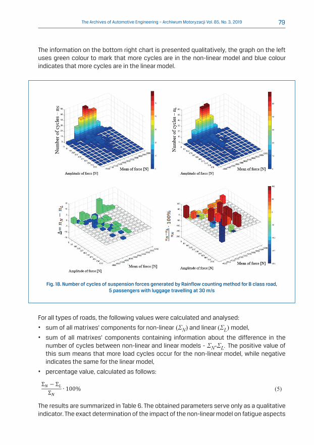
The effects of the implementation of the method of systematization of forces operating in the suspension (described in chapter 3.3) is presented in Figure 18. The results are pre-sented on two-dimensional bar graphs. The x-axis contains information about the average value of the load cycle, the y-axis about amplitude value, while on the z-axis the number of cycles determined from the processed runs by the Rainflow method is shown. The top two graphs present the number of cycles of given amplitude and mean of force for non-linear model on the left and linear model on the right. In the lower part there are graphs contain-ing information about the percentage value calculated by following way:


Fig. 17. The percentage ratio between comfort indexes for different vehicle speeds (C class road,

5 passengers on board)

5.3 Fatigue strength results

The effects of the implementation of the method of systematization of forces operating in the suspension (described in chapter 3.3) is presented in Figure 18. The results are presented on two-dimensional bar graphs. The x-axis contains information about the average value of the load cycle, the y-axis about amplitude value, while on the z-axis the number of cycles determined from the processed runs by the Rainflow method is shown. The top two graphs present the number of cycles of given amplitude and mean of force for non-linear model on the left and linear model on the right. In the lower part there are graphs containing information about the percentage value calculated by following way:

𝑛𝑛𝑁𝑁 𝑘𝑘𝑘𝑘 − 𝑛𝑛L 𝑘𝑘𝑘𝑘𝑛𝑛𝑁𝑁 𝑘𝑘𝑘𝑘

∙ 100% (4)

where:

𝑛𝑛𝑁𝑁 𝑘𝑘𝑘𝑘 – number of cycles defined by Rainflow method for k-th row and i-th column of matrix for non-linear model of suspension;

𝑛𝑛𝐿𝐿 𝑘𝑘𝑘𝑘 – number of cycles defined by Rainflow method for k-th row and i-th column of matrix for linear model of suspension.

The information on the bottom right chart is presented qualitatively, the graph on the left uses green colour to mark that more cycles are in the non-linear model and blue colour indicates that more cycles are in the linear model.

where:

nN ki – number of cycles defined by Rainflow method for k-th row and i-th column of matrix for non-linear model of suspension;

nL ki – number of cycles defined by Rainflow method for k-th row and i-th column of matrix for linear model of suspension.


The information on the bottom right chart is presented qualitatively, the graph on the left uses green colour to mark that more cycles are in the non-linear model and blue colour indicates that more cycles are in the linear model.

Fig. 18. Number of cycles of suspension forces generated by Rainflow counting method for B class road, 5 passengers with luggage travelling at 30 m/s

For all types of roads, the following values were calculated and analysed:

• sum of all matrixes’ components for non-linear (ΣN) and linear (ΣL) model,

• sum of all matrixes’ components containing information about the difference in the number of cycles between non-linear and linear models - ΣN-ΣL. The positive value of this sum means that more load cycles occur for the non-linear model, while negative indicates the same for the linear model,

• percentage value, calculated as follows:


Fig. 18. Number of cycles of suspension forces generated by Rainflow counting method for B class

road, 5 passengers with luggage travelling at 30 m/s

For all types of roads, the following values were calculated and analysed:

• sum of all matrixes’ components for non-linear (Σ𝑁𝑁) and linear (Σ𝐿𝐿) model, • sum of all matrixes’ components containing information about the difference in the number of

cycles between non-linear and linear models - Σ𝑁𝑁 − Σ𝐿𝐿. The positive value of this sum means that more load cycles occur for the non-linear model, while negative indicates the same for the linear model,

• percentage value, calculated as follows: Σ𝑁𝑁 − Σ𝐿𝐿Σ𝑁𝑁

∙ 100% (5)

The results are summarized in Table 6. The obtained parameters serve only as a qualitative indicator. The exact determination of the impact of the non-linear model on fatigue aspects goes beyond the scope of this article. However, as should be noted, the higher number of cycles will result in a significant reduction in fatigue strength, because the relationship between the number of cycles and destructive stresses is strongly non-linear.

Tab. 6. Differences between the number of cycles for non-linear and linear models used in fatigue analysis for different road classes

The results are summarized in Table 6. The obtained parameters serve only as a qualitative indicator. The exact determination of the impact of the non-linear model on fatigue aspects


goes beyond the scope of this article. However, as should be noted, the higher number of cycles will result in a significant reduction in fatigue strength, because the relationship between the number of cycles and destructive stresses is strongly non-linear.

Tab. 6. Differences between the number of cycles for non-linear and linear models used in fatigue analysis for different road classes

Road class Model ΣN ΣN- ΣL

ΣN- ΣL

ΣN

‧ 100%

Class AQuarter 436 cycles 21 cycles +4,8%

Half 429 cycles 49 cycles +11%

Class BQuarter 351 cycles 29 cycles +8,3%

Half 315 cycles 9 cycles +2,8%

Class CQuarter 220 cycles -21 cycles -9,5%

Half 204 cycles -28 cycles -13%

Class DQuarter 147 cycles 33 cycles +22%

Half 159 cycles 40 cycles +25%

The results indicate that more load cycles occur in the non-linear model, which proves that the use of the non-linear model has an impact on durability prediction. Thus, the authors are of the opinion that further research should be undertaken to detail the impact of the non-linear suspension model on the fatigue aspects of components of motor vehicles.

6. Conclusion and further studies

Conducted research included a wide spectrum of possible conditions of use of a typical, middle class passenger car. Based on the gathered data the researchers were able to come up with conclusions, which they used to form some guidelines for when the use of linear or non-linear models is or is not recommended. The specifics though depend on what the person running a simulation wants to achieve.

Simulation made to test ride safety or comfort in most conditions of use can be conducted on simpler linear models. Roads of classes A and B rarely enter the non-linear range of sus-pension work, with the exception of vehicles being heavily loaded in the case of B class road, where the non-linear model might be worth considering. For worse quality roads, especially class D, linear models can yield somewhat satisfactory and realistic results only for best case scenarios, i.e. very low speeds and an almost empty vehicle. Otherwise, the suspension regularly enters non-linear working range. The conclusions reached by the au-thors concerning sprung mass accelerations are in line with the previous works in this fields of study – [16].

If the simulation results are planned to be used for fatigue strength calculations then the use of non-linear models is recommended even more often. High speed vehicle travel even on roads of very high quality (class A) causes not frequent, but present nonetheless loads


in the suspension, which can greatly reduce the life expectancy of said suspension. Not taking those inputs into account can lead to unreliability of suspension elements or even accidents.

Finally, it is worth noting that using linear models does not necessarily mean underesti-mating acceleration or force values, as for some frequencies their values observed were greater than in a non-linear model. It is still more common for the non-linear models to ex-hibit bigger forces, but distortions from reality for both better and worse are unwanted and should be omitted whenever possible.

In the future studies the researchers will continue developing road and vehicle models. Full car model with non-linear spring and damper characteristics is planned and the com-parison of all 3 kinds of vehicle models will be made. The fatigue strength analysis based on the created load spectra will also be conducted. Finally, real life test will take place, and their registered results will be compared with the data from the simulations.

7. NomenclatureDLC dynamic load coefficient

DOF degree of freedom

EL exposure limit

EUSAMA European Shock Absorber Manufacturers Association

FDP fatigue decreased proficiency

FEM finite elements method

IRI international roughness index

PSD power spectral density

RCB reduced comfort boundary

RMS root mean square

RTRRMS response type road roughness measuring system

S-N nominal stress (S) vs number of cycles to failure (N)

SUV sport utility vehicle

References[1] Aghilone G.: Analysis of methods proposed by International Standard ISO 2631 for evaluating the human

exposure to whole-body vibration. Progress in Vibration and Acoustics, 2016, 4(4), 1–13, DOI: 10.12866/J.PIVAA.2016.19.

[2] Bekker H.: 2018 (Full Year) Europe: Best-Selling Car Models. 2019. [Online]. Available: https://www.best-selling-cars.com/europe/2018-full-year-europe-best-selling-car-models-in-the-eu/. [Accessed: 04-Jul-2019].

[3] Bogsjö K., Podgórski K., Rychlik I.: Models for road surface roughness. Vehicle System Dynamics. 2012, 50(5), 725–747, DOI: 10.1080/00423114.2011.637566.

[4] Celko J., Decky M., Kovac M.: An analysis of vehicle – road surface interaction for classification of IRI in the frame of Slovak PMS. Maintenance and reliability, Polish Maintenance society, 2009, 1(41), 15-21.

[5] Doumiati M., Victorino A., Charara A., Lechner D.: Estimation of road profile for vehicle dynamics motion: Experimental validation. Proceedings of the American Control Conference. 2011, 5237–5242, DOI: 10.1109/ACC.2011.5991595.


[6] Dukkipati R.V., Pang J., Qatu M.S., Sheng G., Shuguang Z.: Road Vehicle Dynamic. SAE International. 2008.

[7] Hejman M., Lukes V.: Generation of virtual track profiles using experiments and computer simulations. Journal of Theoretical and Applied Mechanics. 2008, 46(2), 435–442.

[8] Heuler P., Klätschke H.: Generation and use of standardised load spectra and load-time histories. International Journal of Fatigue. 2005, 27(8), 974–990, DOI:10.1016/j.ijfatigue.2004.09.012.

[9] ISO-2631: Mechanical vibration and shock evaluation of human exposure to whole-body vibration. 1997.

[10] Jazar R.N.: Vehicle Dynamics. Theory and Application, Springer, 2008.

[11] Johannesson P. Rychlik I.: Laplace processes for describing road profiles. Procedia Engineering. 2013, 66, 464–473, DOI: 10.1016/j.proeng.2013.12.099.

[12] Johannesson P. Rychlik I.: Modelling of road profiles using roughness indicators. International Journal of Vehicle Design. 2014, 66(4), 317-346, DOI: 10.1504/IJVD.2014.066068.

[13] Kamiński E., Pokorski J.: Teoria samochodu. Dynamika zawieszeń i układów napędowych pojazdów samocho-dowych. WKŁ, Warszawa 1983.

[14] Kropáč O. Múčka P.: Be careful when using the International Roughness Index as an indicator of road uneven-ness. Journal of Sound and Vibration. 2005, 287(4–5), 989–1003, DOI: 10.1016/j.jsv.2005.02.015.

[15] Lozia Z.: Wybrane zagadnienia symulacji cyfrowej procesu hamowania samochodu dwuosiowego na ni-erównej nawierzchni drogi. Politechnika Warszawska, 1985.

[16] Maher D., Young P.: An insight into linear quarter car model accuracy. Vehicle System Dynamics. 2011, 49(3), 463–480, DOI: 10.1080/00423111003631946.

[17] Mattetti M., Molari G., Sedoni E.: Methodology for the realisation of accelerated structural tests on tractors. Biosystems Engineering. 2012, 113(3), 266–271, DOI: 10.1016/j.biosystemseng.2012.08.008.

[18] McGetrick P.J., Kim C.W., Gonzalez A., Obrien E.J.: Dynamic Axle Force and Road Profile Identification Using a Moving Vehicle. International Journal of Architecture, Engineering and Construction. 2013, 2(1), 1–16, DOI: 10.7492/IJAEC.2013.001.

[19] Mitschke M.: Dynamika samochodu t.2 Drgania. WKiŁ. Warszawa 1989.

[20] Mitura A.: Modelowanie drgań nieliniowego zawieszenia pojazdu samochodowego z tłumieniem magnetore-ologicznym: rozprawa doktorska. Politechnika Lubelska, Lublin 2010.

[21] Múčka P.: Simulated Road Profiles According to ISO 8608 in Vibration Analysis. Journal of Testing and Evaluation. 2017, 46(1) 20160265, DOI: 10.1520/JTE20160265.

[22] Múčka P.: Road waviness and the dynamic tyre force. International Journal of Vehicle Design. 2005, 36(2/3), 216-232, DOI: 10.1504/IJVD.2004.005357.

[23] OBrien E.J., McGetrick P.J., González A.: Identification of Road Irregularities via Vehicle Accelerations. Transport Research Arena (TRA 2010), Brussels, Belgium. 2010, 7–10.

[24] Pikosz H. Ślaski G.: Charakterystyki elementów sprężystych i tłumiących zawieszenia samochodu oosob-wego oraz zastępcze charakterystyki ich modeli. Logistyka. 2010, 2.

[25] Rotenberg R.W.: Zawieszenie samochodu. Wydawnictwo Komunikacji i Łączności. 1974.

[26] Savaresi S.M., Poussot-Vassal C., Spelta C., Sename O., Dugard L.: Semi-Active Suspension Control Design for Vehicles. 2010.

[27] Ślaski G.: Studium projektowania zawieszeń samochodowych o zmiennym tłumieniu. Wydawnictwo Politechniki Poznańskiej, Poznań 2012.

[28] Sunder R.: Spectrum load fatigue - Underlying mechanisms and their significance in testing and analysis. International Journal of Fatigue. 2003, 25(9–11), 971–981, DOI: 10.1016/S0142-1123(03)00136-1.

[29] Genta G., Morello L.: The Automotive Chassis. System Design. Springer, New York 2009.

[30] Zdanowicz P., Lozia Z.: Wyznaczenie optymalnej wartości współczynnika asymetrii amortyzatora pasywne-go zawieszenia samochodu z wykorzystaniem modelu „ćwiartki samochodu. Prace. Naukowe. Politechniki. Warszawskiej - Transport. 2017, 119, 249–265.

THE INFLUENCE OF THE CONDITIONS OF USE AND THE TYPE OF ...

Documents

Transcript of THE INFLUENCE OF THE CONDITIONS OF USE AND THE TYPE OF ...